CLASSIC v1.0: the open-source community successor to the Canadian Land Surface Scheme (CLASS) and the Canadian Terrestrial Ecosystem Model (CTEM) – Part 2: Global benchmarking

The Canadian Land Surface Scheme Including Biogeochemical Cycles (CLASSIC) is an open-source community model designed to address research questions that explore the role of the land surface in the global climate system. Here, we evaluate how well CLASSIC reproduces the energy, water, and carbon cycle when forced with quasi-observed meteorological data. Model skill scores summarize how well model output agrees with observation-based reference data across multiple statistical metrics. A lack of agreement may be due to deficiencies in the model, its forcing data, and/or reference data. To address uncertainties in the forcing, we evaluate an ensemble of CLASSIC runs that is based on three meteorological data sets. To account for observational uncertainty, we compute benchmark skill scores that quantify the level of agreement among independent reference data sets. The benchmark scores demonstrate what score values a model may realistically achieve given the uncertainties in the observations. Our results show that uncertainties associated with the forcing and observations are considerably large. For instance, for 10 out of 19 variables assessed in this study, the sign of the bias changes depending on what forcing and reference data are used. Benchmark scores are much lower than expected, implying large observational uncertainties. Model and benchmark score values are mostly similar, indicating that CLASSIC performs well when considering observational uncertainty. Future model development should address (i) a positive albedo bias and resulting shortwave radiation bias in parts of the Northern Hemisphere (NH) extratropics and Tibetan Plateau, (ii) an out-of-phase seasonal gross primary productivity cycle in the humid tropics of South America and Africa, (iii) a lacking spatial correlation of annual mean net ecosystem exchange with site-level measurements, (iv) an underestimation of fractional area burned and corresponding emissions in the boreal forests, (v) a negative soil organic carbon bias in high latitudes, and (vi) a time lag in seasonal leaf area index maxima in parts of the NH extratropics. Our results will serve as a baseline for guiding and monitoring future CLASSIC development.

1 Introduction

The land surface interacts with the atmosphere through fluxes of momentum, radiation, heat, and mass, the latter including water, trace gases, and aerosols. Land surface models (LSMs) have been developed to simulate these fluxes in global climate models. Early LSMs consisted of simple aerodynamic bulk transfer formulas with prescribed surface parameters that are uniform across continents (Manabe, 1969; Manabe and Bryan, 1969). Major advancements in LSM development have occurred since then, including the incorporation of (i) vegetation effects on the surface energy balance (Dickinson, 1984), (ii) vegetation phenology (Sellers et al., 1996), (iii) ecological processes (Foley et al., 1996), and (iv) nutrient cycles (Goll et al., 2012).

The Canadian Land Surface Scheme Including Biogeochemical Cycles (CLASSIC; v1.0; Melton et al., 2020) is a state-of-the-art land surface model primarily developed by Environment and Climate Change Canada. CLASSIC is the open-source community model successor to the CLASS-CTEM modeling framework, which consists of the Canadian Land Surface Scheme (CLASS) and the Canadian Terrestrial Ecosystem Model (CTEM). CLASS and CTEM simulate physical and biogeochemical land surface processes, respectively, and together they form the land component of the Canadian Earth System Model (Swart et al., 2019).

Assessing model performance provides invaluable guidance for future model development. Strategies for LSM evaluation have been developed in a number of collaborative research projects, such as the Project for Intercomparison of Land Surface Parameterization Schemes (PILPS) (Henderson-Sellers et al., 1993), the Global Land-Atmosphere Coupling Experiment (GLACE) (Koster et al., 2006), the Protocol for the Analysis of Land Surface Models (PALS), the Land Surface Model Benchmarking Evaluation Project (PLUMBER) (Best et al., 2015), and the International Land Model Benchmarking (ILAMB) project (Collier et al., 2018). The ILAMB approach summarizes model performance across multiple statistical metrics using a dimensionless skill score that ranges from zero to unity, where higher values imply better performance (see Sect. 2 for details).

The ILAMB framework has been adopted by the Global Carbon Project to evaluate the performance of LSMs used for estimating global carbon budgets (Friedlingstein et al., 2019). The project assessed 15 LSMs with respect to gross primary productivity (GPP), ecosystem respiration, net ecosystem exchange (NEE), biomass, soil carbon, leaf area index (LAI), evapotranspiration, and runoff. For CLASS-CTEM, which was one of the 15 models, performance was considerably weaker for LAI and NEE than for other variables. While a low LAI score was also found for most other LSMs, the NEE score was below the multi-model mean value. The variables for which CLASS-CTEM performed best and worst with respect to the multi-model mean were GPP and biomass, respectively. However, skill scores must be interpreted with caution. For instance, low score values may actually reflect uncertainties in model inputs and/or reference data rather than deficiencies in the model. A robust analysis should therefore account for uncertainties associated with the forcing and reference data.

Lawrence et al. (2019) applied ILAMB to quantify how model development affected model performance for the Community Land Model (CLM). While the authors found a general improvement from CLM version 4 to version 5, they also identified variables where model performance would improve or worsen, depending on the choice of reference data. A second source of uncertainty identified by the authors was related to the choice of meteorological forcing. Driving CLM with three different data sets (GSWP3, CRUNCEPv7, and WATCH/WFDEI) showed that model performance was generally better when forcing CLM with the Global Soil Wetness Project forcing data set (GSWP3), and that the uncertainty associated with the forcing is too large to be neglected (Bonan et al., 2019).

A first evaluation of CLASSIC has been presented by Melton et al. (2020), who ran the model for 31 FLUXNET sites using locally observed meteorological data and vegetation composition. Model outputs were compared against observed net surface radiation (RNS), latent heat flux (HFLS), sensible heat flux (HFSS), GPP, ecosystem respiration (RECO), and NEE. Results showed that CLASSIC reproduced the RNS, HFLS, HFSS, GPP, and RECO observations reasonably well. Reproducing NEE fluxes proved to be more challenging. While for some sites modeled NEE fluxes were in good agreement with measurements (e.g. site FI-Hyy; Figs. S22 and S23 in Melton et al., 2020), for most sites NEE differed considerably from observations. Assessing the annual mean NEE value for each station showed that modeled and observed annual mean values were not correlated across stations. The poor model performance for NEE may be related to the fact that the model does not account for the disturbance history nor the climate history of a given site. A comparison between results presented in the present study and Melton et al. (2020) is provided in the Discussion section.

This present paper provides a comprehensive assessment of model performance on a global scale. Our assessment is based on ILAMB's statistical framework, which we implemented in a new R package referred to as the Automated Model Benchmarking R package (AMBER) (Seiler, 2020). The development of AMBER allowed us to tailor the ILAMB approach to CLASSIC model output. The resulting benefits include (i) a seamless data ingestion that does not require any pre-processing, (ii) the ability to evaluate CLASSIC in different simulation modes (i.e. global runs on a regular grid, regional runs on a rotated grid, and site-level runs), (iii) full control on how the statistical framework is implemented, and (iv) the addition of new functionalities. Our analysis pays special attention to how model performance is affected by uncertainties in the forcing and reference data.

The remainder of the paper is organized as follows. Section 2 describes the forcing data, reference data, model structure, and benchmarking approach. Section 3 assesses model performance for an ensemble of three model runs that differ in their meteorological forcing. For most variables, each ensemble member is compared against more than one observation-based reference data set. For each variable, we assess global, zonal, and seasonal biases, as well as root-mean-square errors, time lags in seasonal peaks, interannual variability, spatial patterns, and corresponding skill scores. Furthermore, we compare model skill scores against benchmark scores, which are based on reference data only, to assess the extent to which score values are affected by observational uncertainty. Section 4 elaborates on our principal findings, with a particular focus on LAI and NEE, and the importance of in situ measurements.

2 Methods

2.1 Canadian Land Surface Scheme Including Biogeochemical Cycles (CLASSIC)

CLASSIC is the open-source community model successor to the CLASS-CTEM modeling framework, which consists of the Canadian Land Surface Scheme (CLASS) and the Canadian Terrestrial Ecosystem Model (CTEM). CLASS and CTEM are two fully integrated model components that simulate physical and biogeochemical land surface processes, respectively. A brief outline of these two components is provided next.

CLASSIC's physical component (CLASS) divides the land surface into four possible subareas, namely bare ground, ground covered by snow, ground covered by canopy, and snow covered by canopy. The model solves the energy balance for the canopy layer and underlying ground, separately. The canopy consists of a single layer and is for the results presented here composed of four plant functional types (PFTs), namely needleleaf trees, broadleaf trees, grasses, and crops. The model output evaluated here is from the offline mode in which we use 20 soil layers ranging from 10 layers of 0.1 m thickness, gradually increasing to a 30 m thick layer for a total ground depth of over 61 m. Water fluxes are calculated for soil layers within the permeable soil depth of the ground column but not the underlying bedrock layers, whereas temperatures are calculated for both soil and bedrock layers. Also calculated are the temperature, mass, albedo, and density of the single-layer snowpack, the temperature and interception and storage of rain and snow on the vegetation canopy, and the temperature and depth of ponded water on the ground surface.

CLASSIC's biogeochemical component (CTEM) is a dynamic vegetation model coupled to CLASS. CLASS provides CTEM physical land surface information, including soil moisture, soil temperature and net radiation. CTEM uses this information to simulate photosynthesis in response to atmospheric CO₂ concentration. CTEM considers three live vegetation components (leaves, stem, and roots) and two dead carbon pools (litter and soil). These five carbon pools are tracked, in the default CLASSIC configuration used here, for nine PFTs that map directly onto the four PFTs used by CLASS. Needleleaf trees are divided into their deciduous and evergreen types, broadleaf trees are divided into cold and drought deciduous and evergreen types, and crops and grasses are divided based on their photosynthetic pathways into C₃ and C₄ versions. In this study, the spatial distribution of PFTs has been prescribed to reduce the number of possible causes for model biases. The prognostic carbon masses of leaf, stem, and root simulated by CTEM are used to calculate the structural vegetation characteristics required by CLASS. The main processes simulated by CTEM include photosynthesis, canopy conductance, tissue turnover, allocation of carbon, and phenology (Arora and Boer, 2005b); dynamic root distribution (Arora and Boer, 2003); maintenance, growth, and heterotrophic respiration (Melton et al., 2015); wildfires (Arora and Boer, 2005a; Arora and Melton, 2018); competition for space between PFTs (Arora and Boer, 2006; Melton and Arora, 2016), and land use change (Arora and Boer, 2010). For the purpose of this study, CLASSIC's recently added nitrogen cycle has been turned off (Asaadi and Arora, 2021). A more detailed description of the model and its history is documented in Melton et al. (2020). Details on the computation of radiation fluxes, surface albedo, heat fluxes, LAI, GPP, ecosystem respiration, and biomass are provided in the Appendix.

Pastorello et al. (2017)Dai and Trenberth (2002)Mortimer et al. (2020)Garrigues et al. (2008)Iio and Ito (2014)Schepaschenko et al. (2019)Strahler et al. (1999)Zhang et al. (2017)Myneni et al. (2002)Claverie et al. (2016)Kato et al. (2013)Stackhouse et al. (2011)Li and Xiao (2019)Jung et al. (2019)Jung et al. (2020)Hobeichi et al. (2019)Liu et al. (2011)Mudryk (2020)Brown et al. (2003)Brun et al. (2013)Takala et al. (2011)Gelaro et al. (2017)Giglio et al. (2010)Chuvieco et al. (2018)Jacobson et al. (2020)Avitabile et al. (2016)Santoro et al. (2015)Saatchi et al. (2011)Wieder (2014)Todd-Brown et al. (2013)

Table 1 Observation-based reference data used for model evaluation. Meanings of acronyms are provided in Sect. 2. N/A: not applicable.

2.2 Meteorological forcing

Meteorological inputs required by CLASSIC include surface downwelling shortwave (SW) and longwave (LW) radiation, near-surface air temperature, precipitation, near-surface specific humidity, surface pressure, and near-surface horizontal wind speed. Model outputs are potentially sensitive to uncertainties in the meteorological forcing. To account for this uncertainty, we drive CLASSIC with three different quasi-observed meteorological data sets, namely the Climate Research Unit – National Centers for Environmental Prediction version 8 (CRUNCEP; 1901–2016; Viovy, 2018), the Climate Research Unit – Japanese 55-year Reanalysis version 2.0 (CRUJRAv2; 1901–2017; Harris et al., 2014; Kobayashi et al., 2015), and the Global Soil Wetness Project Phase 3 (GSWP3) – WFDE5 over land merged with ERA5 over the ocean (W5E5) (GSWP3W5E5; 1901–2016; ISIMIP, 2020). All meteorological forcings are disaggregated from 6-hourly to half-hourly time steps, following the methodology by Melton and Arora (2016).

Zonal mean values suggest that all three forcings are relatively consistent (Fig. A1). The corresponding global mean values for CRUJRAv2, GSWP3W5E5, and CRUNCEP are 182, 178, and 183 W m⁻² for downwelling SW radiation, 304, 309, and 300 W m⁻² for downwelling LW radiation, 10 ^∘C for near-surface air temperature (all three forcings), 59, 64, and 60 mm per month precipitation, 6.9, 7.4, and $\mathrm{6.9}\times {\mathrm{10}}^{-\mathrm{3}}$ kg kg⁻¹ for specific humidity, 947, 948, and 950 hPa surface pressure, and 2.6, 3.3, and 2.6 m s⁻¹ horizontal wind speed, respectively. With the exception of surface pressure, the data from CRUJRAv2 and GSWP3W5E5 tend to be more similar compared to CRUNCEP.

2.3 Simulation protocol

Our simulations are based on the trends in the land carbon cycle project (TRENDY) simulation protocol with time-varying CO₂, climate, and land use (S3) (Friedlingstein et al., 2019). The protocol consists of a spinup for the year 1700 and two transient runs for the periods 1701–1900 and 1901–2016, respectively. The spinup uses a constant atmospheric CO₂ concentration of 276.59 ppm, climate data from the early decades of the 20th century (i.e. 1901–1920), and a land use map with constant crops and pasture distribution. The first transient run uses the same climate as for the spinup but time-varying CO₂ concentrations and land use for the 1701–1900 period. The second transient run uses time-varying CO₂, climate, and land use for the 1901–2017 period.

Figure 1 Biases when comparing CLASSIC forced with CRUJRAv2 against in situ measurements of (a) net surface radiation, (b) latent heat flux, (c) sensible heat flux, (d) soil heat flux, (e) streamflow, and (f) snow water equivalent. Measurements located in the same model grid cell were merged. Upward- and downward-pointing triangles indicate positive and negative biases, respectively.

Figure 2 Same as Fig. 1 but for (a) gross primary productivity, (b) ecosystem respiration, (c) net ecosystem exchange, (d) above-ground biomass, (e) leaf area index, and (f) maximum leaf area index.

2.4 Reference data

Model outputs are evaluated against in situ observations and globally gridded observation-based reference data (Table 1). The reference database covers 19 variables that form part of the energy, water, and carbon cycle. While most data sets consist of monthly mean values, some are assessed on an annual timescale (streamflow) or present a snapshot in time (vegetation biomass, organic soil carbon mass, and in situ LAI measurements provided by the Oak Ridge National Laboratory). All gridded reference data are spatially interpolated to the spatial resolution of a CLASSIC grid cell ($\mathrm{2.8125}{}^{\circ }\times \mathrm{2.8125}{}^{\circ }$). In situ observations that fall into the same model grid cell are averaged prior to the comparison against model output. In most cases, the evaluation is based on the grid cell value, which reflects the average conditions across all land cover types located in a grid cell. For above-ground biomass, however, a comparison between the grid cell value and forest inventory data is not ideal, as the latter provides biomass estimates for trees only. We therefore only consider biomass simulated for trees when evaluating model results against forest inventory data. Details on each reference data set are provided next.

2.4.1 In situ observations

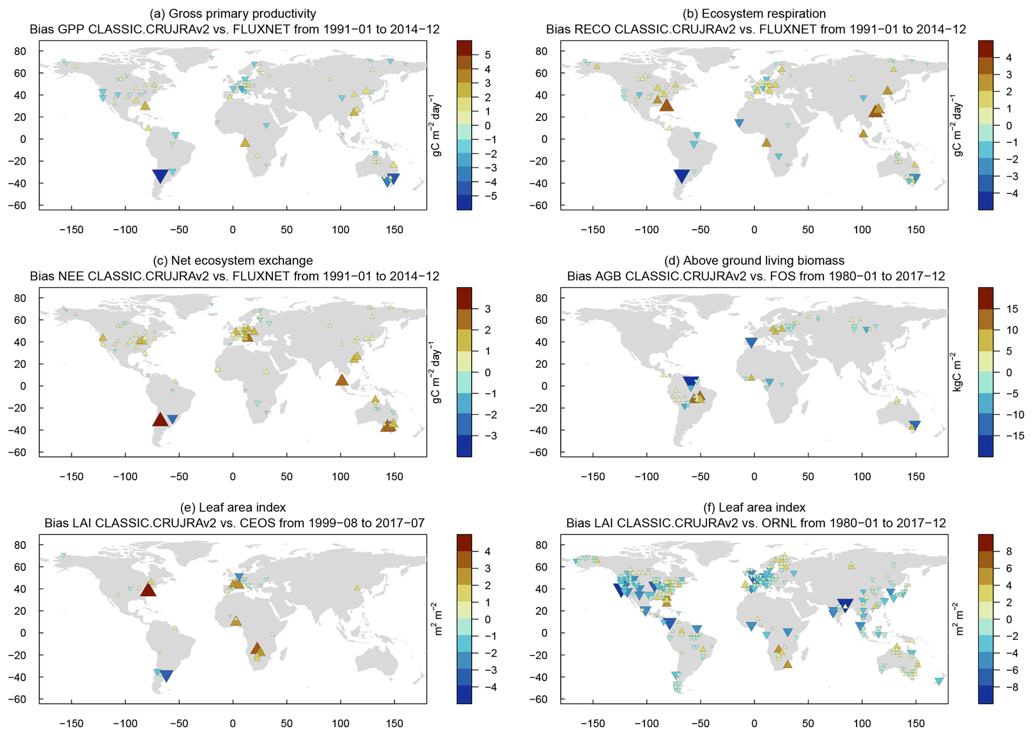
The FLUXNET2015 database includes 204 eddy covariance sites with measurements overlapping during the years 1997 and 2014 (Pastorello et al., 2017) (Table 1). The corresponding variables include RNS, HFLS, HFSS, soil heat flux (HFG) (Fig. 1a–d), GPP, RECO, and NEE (Fig. 2a–c).

Streamflow gauge records are provided by the Global Runoff Data Centre (GRDC) for the world's 50 largest basins (Dai and Trenberth, 2002) (Fig. 1e). Measurements were made sometime between 1980 and 2010, depending on the basin.

Mortimer et al. (2020) compiled manual gravimetric measurements of snow water equivalent (SNW) collected from 3271 sites located between 42 and 83^∘ N for the 1970–2017 period (Fig. 1f).

Above-ground biomass (AGB) measurements were provided by the Forest Observation System (FOS) who compiled measurements from 274 permanent research plots (Schepaschenko et al., 2019) (Fig. 2d). Measurements are based on allometric relations and were made between 1999 and 2018, depending on the inventory plot.

LAI observations are taken from the Committee on Earth Observation Satellites (CEOS) (Garrigues et al., 2008) and the Oak Ridge National Laboratory (ORNL) (Iio and Ito, 2014) (Fig. 2e and f). The CEOS database consists of 141 sites with measurements during the 1999–2017 period. The values are based on a transfer function that upscales ground LAI measurements to a moderate-resolution grid cell using high-spatial-resolution surface reflectances. The ORNL data set contains a total of 2653 measurements compiled from literature that was published between 1932 and 2012. The values present site-specific maximum ground LAI measurements.

2.4.2 Globally gridded reference data

The Moderate Resolution Imaging Spectroradiometer (MODIS) provides globally gridded data sets for white-sky surface albedo (2000–2014), GPP (2000–2016), and LAI (2000–2017). The white-sky albedo (MCD43C3 v006) integrates the bidirectional reflectance distribution function (BRDF) over all viewing and irradiance directions. The resulting albedo values are properties of the surface that do not depend on the state of the atmosphere (Strahler et al., 1999). Only data with quality flags of less than 3 and solar zenith angles of less than 70^∘ were considered. Evaluating MODIS V6 surface albedo against in situ measurements shows that biases for the high-quality data (full inversion) range from −0.0061 in needleleaf forests to 0.0023 in deserts (Wang et al., 2018).

MODIS-based GPP is provided by Zhang et al. (2017) for the period 2000–2017. The data set estimates GPP as the product of light absorption by chlorophyll and the efficiency that converts the absorbed energy to carbon fixed by plants through photosynthesis. The required inputs include a range of MODIS products (surface temperature, land surface water index, enhanced vegetation index, and land cover classification), as well as air temperature and radiation fluxes from NCEP Reanalysis II (Kanamitsu et al., 2002).

MODIS LAI (MOD15A2H, Collection 6; Myneni et al., 2015) is based on the inversion of a three-dimensional canopy radiative transfer model that simulates surface reflectance from canopy structural characteristics (Knyazikhin et al., 1998). The inversion approach causes LAI to be very sensitive to uncertainties in surface reflectance. Those uncertainties may occur due to calibration errors, residual atmospheric and cloud contamination, background underneath the canopy, topography, view-illumination geometry effects, and reflectance saturation in dense canopies (Garrigues et al., 2008). MODIS LAI uncertainties of annual mean values range from 23 % to 38 % across biomes, with a global mean value of 27 % for MODIS LAI Collection 5 (Fang et al., 2012).

A second set of globally gridded LAI was provided by Claverie et al. (2016) for the period 1982–2010. This data set is based on an artificial neural network (ANN) that relates LAI to surface reflectance from the Advanced Very High Resolution Radiometer (AVHRR). The ANN was calibrated with LAI from MODIS (MCD15A2) and in situ LAI measurements from BELMANIP2 (445 sites; Baret et al., 2006). The performance of the algorithm was assessed against in situ observations from the DIRECT database (113; Garrigues et al., 2008).

The Clouds and the Earth's Radiant Energy System (CERES) provides globally gridded SW and LW radiation fluxes at the surface under all-sky conditions for the period 2000–2012 (Kato et al., 2013). The data set is based on a radiative transfer model that uses satellite-retrieved surface, cloud, and aerosol properties as inputs. The values of these inputs are adjusted within their uncertainty ranges to obtain irradiance values at the top of the atmosphere that are consistent with observations.

The Global Energy and Water Exchanges Surface Radiation Budget (GEWEXSRB) release 3.0 (Stackhouse et al., 2011) provides globally gridded SW and LW radiation fluxes at the surface under all-sky conditions for the period 1984–2007. The data set is based on a radiative transfer model developed by Pinker and Laszlo (1992), which is driven with satellite observations (cloud parameters and ozone fields) and reanalysis data (Stackhouse et al., 2011). The algorithm scales spectral surface albedos of 12 surface types in such a way that the resulting clear-sky composite broadband top-of-the-atmosphere albedo is consistent with observations from the International Satellite Cloud Climatology Project (Zhang et al., 2019). Surface fluxes have been evaluated against ground-based measurements from sources that include the Baseline Surface Radiation Network and the Global Energy Balance Archive.

The GOSIF data provided by Li and Xiao (2019) are based on linear correlations between solar-induced chlorophyll fluorescence (SIF) soundings from the Orbiting Carbon Observatory-2 (OCO-2) and GPP measurements from 91 eddy covariance measurements sites from FLUXNET.

The FluxCom data set is an ensemble of globally gridded energy fluxes (HFLS, HFSS, and RNS from 2001 to 2013) and carbon fluxes (GPP, NEE, and RECO from 1980 to 2013). Using a range of machine learning methods, FluxCom upscales FLUXNET observations, where remote sensing data and meteorological data serve as global predictors. The former includes land surface temperature (LST; MOD11A226), land cover (MCD12Q127), fraction of absorbed photosynthetically active radiation by a canopy (fPAR; MOD15A228), and BRDF-corrected reflectances (MCD43B429) from MODIS. Meteorological data employed by FluxCom were taken from the WATCH Forcing Data ERA-Interim (WFDEI), Global Soil Wetness Project 3 (GSWP), CRUNCEPv837, Global Precipitation Climatology Project (GPCP), and CERES. The FluxCom values used in the present study are the median values computed over the FluxCom ensembles.

The Conserving Land-Atmosphere Synthesis Suite (CLASSr) provides globally gridded estimates of net surface radiation, latent heat flux, sensible heat flux, soil heat flux, and runoff for the 2003–2009 period (Hobeichi et al., 2019). Each variable presents a weighted mean computed from multiple data products that are, to some extent, observation based. The data are observationally constrained with in situ measurements, and each term is adjusted to allow for energy and water balance closure. Net surface radiation, latent heat flux, and sensible heat flux are based on blending data from remote sensing, reanalysis, and land surface models. Soil heat flux estimates are based on reanalysis and land surface models, and runoff is derived from land surface models and hydrological models. The original acronym for the Conserving Land-Atmosphere Synthesis Suite is CLASS. However, in the present paper, we use the acronym CLASSr instead to avoid confusion with the Canadian Land Surface Scheme acronym.

Globally gridded soil moisture estimates provided by Liu et al. (2011) are based on the retrieval characteristics of passive (Advanced Microwave Scanning Radiometer – Earth Observing System; AMSR-E) and active (Advanced Scatterometer; ASCAT) microwave satellite data. Remotely sensed estimates are rescaled using the Noah land surface model (Niu et al., 2011) and evaluated with in situ measurements from the International Soil Moisture Network (Dorigo et al., 2011). Values represent conditions of the first 10 cm of the top soil layer.

Gridded estimates of snow water equivalent for the Northern Hemisphere (NH) are provided by Mudryk (2020). The blended data set is derived from four sources, including a satellite passive microwave radiometer data set (GlobSnow GS3; Takala et al., 2011), reanalysis data (Modern-Era Retrospective analysis for Research and Applications, version 2 – MERRA-2; Gelaro et al., 2017), a temperature index model by Brown et al. (2003), and a physical snowpack model referred to as Crocus (Brun et al., 2013). The present study evaluates model output against the blended product, referred to as ECCC, as well as its four sources.

Global maps of monthly burned area were taken from the fourth generation of the Global Fire Emissions Database (GFED4; Giglio et al., 2010). The data are based on the 500 m Collection 5.1 MODIS direct broadcast (DB) burned-area product (MCD64A1) using the MODIS DB burned-area mapping algorithm by Giglio et al. (2009). The data set has been evaluated against high-resolution Landsat imagery for locations in southern Africa, Siberia, central Asia, Alaska, and the western conterminous United States.

A second data set of monthly burned area is provided by the Fire Disturbance Project of the European Space Agency's Climate Change Initiative program (Chuvieco et al., 2018). This data set was generated from the MODIS red and near-infrared reflectances (MOD09GQ and MCD14ML, both from Collection 6) and thermal anomaly data (MCD14ML). The employed algorithm identifies those grid cells where the presence of wildfires is most evident and then searches for wildfires in close proximity to those grid cells.

CarbonTracker (CT2019) is an inversion model that attempts to reproduce observed atmospheric CO₂ concentrations by adjusting CO₂ fluxes at the surface. The initial states of terrestrial fluxes are obtained from the Carnegie–Ames–Stanford approach (CASA) biogeochemical model (Potter et al., 1993). Fluxes associated with biomass burning are taken from GFED4S. Observations consist of air samples from 460 sites provided by the GLOBALVIEW+ data product version 5.0 (Masarie et al., 2014). While CT2019 is continuously updated, the period considered in this study ranges from 2000 to 2017.

Globally gridded above-ground biomass estimates are provided by GEOCARBON, which is based on a boreal forest biomass map by Santoro et al. (2015) and two pan-tropical biomass maps from Avitabile et al. (2016) and Saatchi et al. (2011). The GEOCARBON map covers only areas that are dominated by trees in the Global Land Cover 2000 map (GLC2000; Bartholome and Belward, 2005). The boreal biomass estimates are based on radar imagery provided by the Envisat Advanced Synthetic Aperture Radar (ASAR). The pan-tropical biomass maps are based on light detection and ranging (lidar) observations that were calibrated with in situ measurements of tree allometry. Baccini et al. (2012) upscaled data using a random forest machine learning algorithm and satellite imagery, including the MODIS nadir BRDF-adjusted reflectance (NBAR), MODIS land surface temperature, and Shuttle Radar Topography Mission (SRTM) digital elevation data. Saatchi et al. (2011) upscaled in situ measurements using a machine learning algorithm (maximum entropy approach) and satellite imagery, including the MODIS normalized difference vegetation index (NDVI) and LAI products, global quick scatterometer (QSCAT), and SRTM digital elevation data. Note that we also used the Saatchi et al. (2011) data on their own to evaluate vegetation carbon in the tropics.

The Harmonized World Soil Database (HWSD) provided by the Food and Agriculture Organization (FAO) combines existing regional and national updates of soil information worldwide with the information contained by the FAO Soil Map of the World (Wieder, 2014). The data were processed by Todd-Brown et al. (2013), who computed soil carbon stocks from bulk densities and organic carbon concentrations given in the HWSD for the top 1 m of soil at a $\mathrm{0.5}{}^{\circ }\times \mathrm{0.5}{}^{\circ }$ resolution.

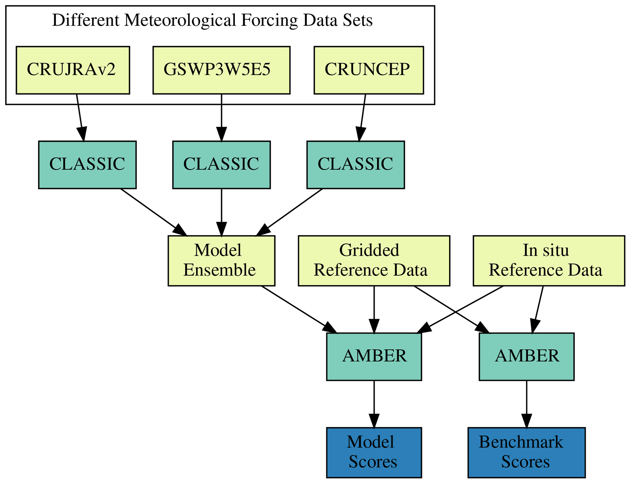
Figure 3 Experimental setup, where yellow boxes refer to data, green boxes to algorithms, and blue boxes to analysis output.

2.5 Automated Model Benchmarking R package (AMBER)

The Automated Model Benchmarking R package (AMBER; version 1.1.0) quantifies model performance using a skill score system originally developed by Collier et al. (2018). The method employs five scores that assess the model's bias (S_bias), root-mean-square error (S_rmse), seasonality (S_phase), interannual variability (S_iav), and spatial distribution (S_dist). The main steps for computing a score usually include (i) computing a dimensionless statistical metric, (ii) scaling this metric onto a unit interval, and (iii) computing a spatial mean. All scores are dimensionless and range from 0 to 1, where increasing values imply better performance. These properties allow us to average skill scores across different statistical metrics in order to obtain an overall score for each variable (S_overall).

Figure 3 provides an overview of our experimental setup. As a first step, we create a small model ensemble by driving CLASSIC with three different meteorological data sets. The purpose of the ensemble is to determine the sensitivity of model performance to uncertainties in the meteorological forcing. Next, we evaluate each ensemble member using AMBER. The resulting model scores express how well model and reference data agree. A low score, however, does not necessarily imply poor model performance, as the lack of agreement may also be due to uncertainties in the forcing data and/or reference data. To assess to what extent model scores are affected by observational uncertainties, we also run AMBER with reference data only. The resulting benchmark scores quantify the level of agreement among different reference data sets. Comparing model scores against benchmark scores then shows how well CLASSIC performs relative to the performance of a reference data set. The remaining part of this section documents the details of the skill scores employed by AMBER.

2.5.1 Bias score (S_bias)

The bias is defined as the difference between the time-mean values of model and reference data:

$$\begin{array}{}\text{(1)}& \text{bias}(\mathit{\lambda },\mathit{\varphi })=\stackrel{\mathrm{‾}}{v_{\text{mod}}}(\mathit{\lambda },\mathit{\varphi })-\stackrel{\mathrm{‾}}{v_{\text{ref}}}(\mathit{\lambda },\mathit{\varphi }),\end{array}$$

where $\stackrel{\mathrm{‾}}{v_{\text{mod}}}(\mathit{\lambda },\mathit{\varphi })$ and $\stackrel{\mathrm{‾}}{v_{\text{mod}}}(\mathit{\lambda },\mathit{\varphi })$ are the mean values in time (t) of a variable v as a function of longitude λ and latitude ϕ for model and reference data, respectively. Nondimensionalization is achieved by dividing the bias by the standard deviation of the reference data (σ_ref):

$$\begin{array}{}\text{(2)}& {\mathit{\epsilon }}_{\text{bias}}(\mathit{\lambda },\mathit{\varphi })=\left|\text{bias}(\mathit{\lambda },\mathit{\varphi })\right|/{\mathit{\sigma }}_{\text{ref}}(\mathit{\lambda },\mathit{\varphi }).\end{array}$$

Note that ε_bias is always positive, as it uses the absolute value of the bias. For evaluations against streamflow measurements, the bias is divided by the annual mean rather than the standard deviation of the reference data. This is because we assess streamflow on an annual rather than monthly basis, implying that the corresponding standard deviation is small. The same approach is applied to soil carbon and biomass, whose reference data provide a static snapshot in time. In both of these cases, ε_bias(λ,ϕ) becomes

$$\begin{array}{}\text{(3)}& {\mathit{\epsilon }}_{\text{bias}}(\mathit{\lambda },\mathit{\varphi })=\left|\text{bias}(\mathit{\lambda },\mathit{\varphi })\right|/\stackrel{\mathrm{‾}}{v_{\text{ref}}}(\mathit{\lambda },\mathit{\varphi }).\end{array}$$

A bias score that scales from 0 to 1 is calculated next:

$$\begin{array}{}\text{(4)}& s_{\text{bias}}(\mathit{\lambda },\mathit{\varphi })=e^{-{\mathit{\epsilon }}_{\text{bias}}(\mathit{\lambda },\mathit{\varphi })}.\end{array}$$

While small relative errors yield score values close to 1, large relative errors cause score values to approach 0 (Fig. 4a). Taking the mean of s_bias across all latitudes and longitudes, denoted by a double bar over a variable, leads to the scalar score:

$$\begin{array}{}\text{(5)}& S_{\text{bias}}=\stackrel{\mathrm{‾}}{\stackrel{\mathrm{‾}}{s_{\text{bias}}}}(\mathit{\lambda },\mathit{\varphi }).\end{array}$$

2.5.2 Root-mean-square-error score (S_rmse)

While the bias assesses the difference between time-mean values, the root-mean-square error (rmse) is concerned with the residuals of the modeled and observed time series:

$$\begin{array}{}\text{(6)}& \begin{array}{rl}& \text{rmse}(\mathit{\lambda },\mathit{\varphi })=\\ & \sqrt{{\displaystyle \frac{\mathrm{1}}{t_{\text{f}}-t_{\mathrm{0}}}}\underset{t_{\mathrm{0}}}{\overset{t_{\text{f}}}{\int }}\left(v_{\text{mod}}\right(t,\mathit{\lambda },\mathit{\varphi })-v_{\text{ref}}(t,\mathit{\lambda },\mathit{\varphi }){)}^{\mathrm{2}}\text{d}t},\end{array}\end{array}$$

where t₀ and t_f are the initial and final time steps, respectively (Fig. A2a and c). A similar metric is the centralized rmse (crmse), which is based on the residuals of the anomalies:

$$\begin{array}{}\text{(7)}& \begin{array}{rl}& \text{crmse}(\mathit{\lambda },\mathit{\varphi })=\\ & \sqrt{{\displaystyle \frac{\mathrm{1}}{t_{\text{f}}-t_{\mathrm{0}}}}\underset{t_{\mathrm{0}}}{\overset{t_{\text{f}}}{\int }}\left[\right(v_{\text{mod}}(t,\mathit{\lambda },\mathit{\varphi })-\stackrel{\mathrm{‾}}{v_{\text{mod}}}(\mathit{\lambda },\mathit{\varphi }))-(v_{\text{ref}}(t,\mathit{\lambda },\mathit{\varphi })-\stackrel{\mathrm{‾}}{v_{\text{ref}}}(\mathit{\lambda },\mathit{\varphi })){]}^{\mathrm{2}}\text{d}t}.\end{array}\end{array}$$

The crmse therefore assesses residuals that have been bias corrected (Fig. A2c and e). Since we already assessed the model's bias through S_bias, it is convenient to assess the residuals using crmse rather than rmse. In a similar fashion to the bias, we then compute a relative error:

$$\begin{array}{}\text{(8)}& {\mathit{\epsilon }}_{\text{rmse}}(\mathit{\lambda },\mathit{\varphi })=\text{crmse}(\mathit{\lambda },\mathit{\varphi })/{\mathit{\sigma }}_{\text{ref}}(\mathit{\lambda },\mathit{\varphi }),\end{array}$$

scale this error onto a unit interval (Fig. 4a):

$$\begin{array}{}\text{(9)}& s_{\text{rmse}}(\mathit{\lambda },\mathit{\varphi })=e^{-{\mathit{\epsilon }}_{\text{rmse}}(\mathit{\lambda },\mathit{\varphi })},\end{array}$$

and compute the spatial mean:

$$\begin{array}{}\text{(10)}& S_{\text{rmse}}=\stackrel{\mathrm{‾}}{\stackrel{\mathrm{‾}}{s_{\text{rmse}}}}.\end{array}$$

2.5.3 Phase score (S_phase)

The skill score S_phase assesses how well the model reproduces the seasonality of a variable by computing the time difference (θ(λ,ϕ)) between modeled and observed maxima of the climatological mean cycle:

$$\begin{array}{}\text{(11)}& \mathit{\theta }(\mathit{\lambda },\mathit{\varphi })=max\left(c_{\text{mod}}\right(t,\mathit{\lambda },\mathit{\varphi }\left)\right)-max\left(c_{\text{ref}}\right(t,\mathit{\lambda },\mathit{\varphi }\left)\right),\end{array}$$

where c_mod and c_ref are the climatological mean cycle of the model and reference data, respectively (Fig. A2b). This time difference is then scaled from 0 to 1 based on the consideration that the maximum possible time difference is 6 months (Fig. 4b):

$$\begin{array}{}\text{(12)}& s_{\text{phase}}(\mathit{\lambda },\mathit{\varphi })={\displaystyle \frac{\mathrm{1}}{\mathrm{2}}}\left[\mathrm{1}+\cos \left({\displaystyle \frac{\mathrm{2}\mathit{\pi }\mathit{\theta }(\mathit{\lambda },\mathit{\varphi })}{\mathrm{365}}}\right)\right].\end{array}$$

The spatial mean of s_phase then leads to the scalar score:

$$\begin{array}{}\text{(13)}& S_{\text{phase}}=\stackrel{\mathrm{‾}}{\stackrel{\mathrm{‾}}{s_{\text{phase}}}}.\end{array}$$

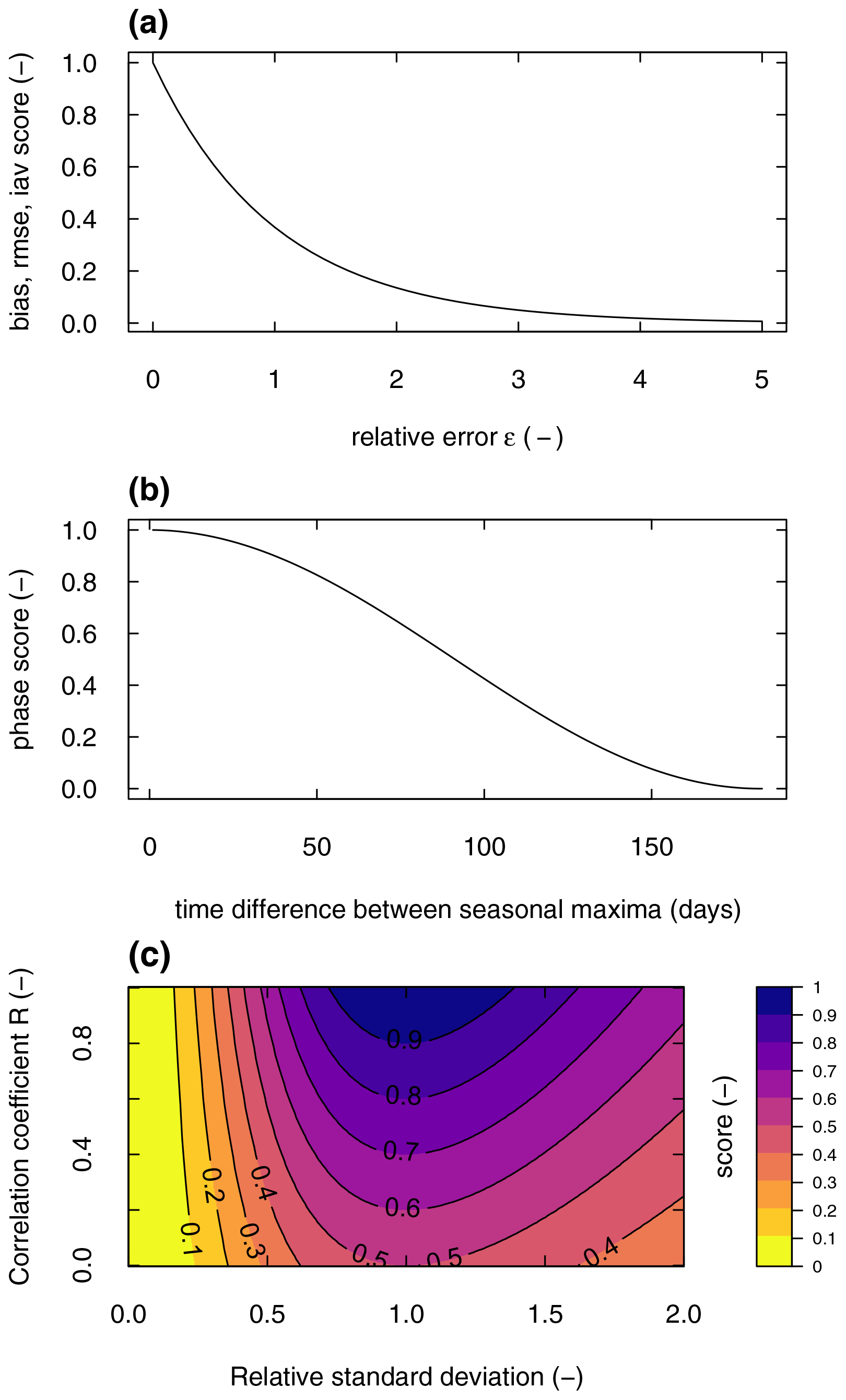
Figure 4 Score functions for (a) bias, root-mean-square error, and interannual variability, (b) seasonality, and (c) spatial distribution.

2.5.4 Interannual variability score (S_iav)

The skill score S_iav quantifies how well the model reproduces patterns of interannual variability. This score is based on data where the seasonal cycle (c_mod and c_ref) has been removed (Fig. A2d and f):

$$\begin{array}{}\text{(14)}& \begin{array}{rl}& {\text{iav}}_{\text{mod}}(\mathit{\lambda },\mathit{\varphi })=\\ & \sqrt{{\displaystyle \frac{\mathrm{1}}{t_{\text{f}}-t_{\mathrm{0}}}}\underset{t_{\mathrm{0}}}{\overset{t_{\text{f}}}{\int }}\left(v_{\text{mod}}\right(t,\mathit{\lambda },\mathit{\varphi })-c_{\text{mod}}(t,\mathit{\lambda },\mathit{\varphi }){)}^{\mathrm{2}}\text{d}t},\end{array}\end{array}$$

$$\begin{array}{}\text{(15)}& {\text{iav}}_{\text{ref}}(\mathit{\lambda },\mathit{\varphi })=\sqrt{{\displaystyle \frac{\mathrm{1}}{t_{\text{f}}-t_{\mathrm{0}}}}\underset{t_{\mathrm{0}}}{\overset{t_{\text{f}}}{\int }}\left(v_{\text{ref}}\right(t,\mathit{\lambda },\mathit{\varphi })-c_{\text{ref}}(t,\mathit{\lambda },\mathit{\varphi }){)}^{\mathrm{2}}\text{d}t}.\end{array}$$

The relative error, nondimensionalization, and spatial mean are computed next (Fig. 4a):

$$\begin{array}{}\text{(16)}& {\mathit{\epsilon }}_{\text{iav}}=\left|\left({\text{iav}}_{\text{mod}}\right(\mathit{\lambda },\mathit{\varphi })-{\text{iav}}_{\text{ref}}(\mathit{\lambda },\mathit{\varphi }\left)\right)\right|/{\text{iav}}_{\text{ref}}(\mathit{\lambda },\mathit{\varphi }),\end{array}$$

$$\begin{array}{}\text{(17)}& s_{\text{iav}}(\mathit{\lambda },\mathit{\varphi })=e^{-{\mathit{\epsilon }}_{\text{iav}}(\mathit{\lambda },\mathit{\varphi })},\end{array}$$

$$\begin{array}{}\text{(18)}& S_{\text{iav}}=\stackrel{\mathrm{‾}}{\stackrel{\mathrm{‾}}{s_{\text{iav}}}}.\end{array}$$

2.5.5 Spatial distribution score (S_dist)

The spatial distribution score S_dist assesses how well the model reproduces the spatial pattern of a variable. The score considers the correlation coefficient R and the relative standard deviation σ between $\stackrel{\mathrm{‾}}{v_{\text{mod}}}(\mathit{\lambda },\mathit{\varphi })$ and $\stackrel{\mathrm{‾}}{v_{\text{ref}}}(\mathit{\lambda },\mathit{\varphi })$. The score S_dist increases from 0 to 1, the closer R and σ approach a value of 1 (Fig. 4c). No spatial integration is required, as this calculation yields a single value:

$$\begin{array}{}\text{(19)}& S_{\text{dist}}=\mathrm{2}(\mathrm{1}+R){\left(\mathit{\sigma }+{\displaystyle \frac{\mathrm{1}}{\mathit{\sigma }}}\right)}^{-\mathrm{2}},\end{array}$$

where σ is the ratio between the standard deviation of the model and reference data:

$$\begin{array}{}\text{(20)}& \mathit{\sigma }={\mathit{\sigma }}_{\stackrel{\mathrm{‾}}{v_{\text{mod}}}}/{\mathit{\sigma }}_{\stackrel{\mathrm{‾}}{v_{\text{ref}}}}.\end{array}$$

2.5.6 Overall score (S_overall)

As a final step, scores are averaged to obtain an overall score:

$$\begin{array}{}\text{(21)}& S_{\text{overall}}={\displaystyle \frac{S_{\text{bias}}+\mathrm{2}{S}_{\text{rmse}}+S_{\text{phase}}+S_{\text{iav}}+S_{\text{dist}}}{\mathrm{1}+\mathrm{2}+\mathrm{1}+\mathrm{1}+\mathrm{1}}}.\end{array}$$

Note that S_rmse is weighted by a factor of 2, which emphasizes its importance.

Table 2 Qualitative assessment of global mean biases. Variables for which positive and negative mean biases are found are denoted with ±. Biases that have a consistent sign across all evaluations but are smaller than ±5 % are marked with ≤5 %. Larger systematic biases are marked with + or −. Numbers provided for each of the in situ reference data refer to the number of grid cells involved.

3 Results

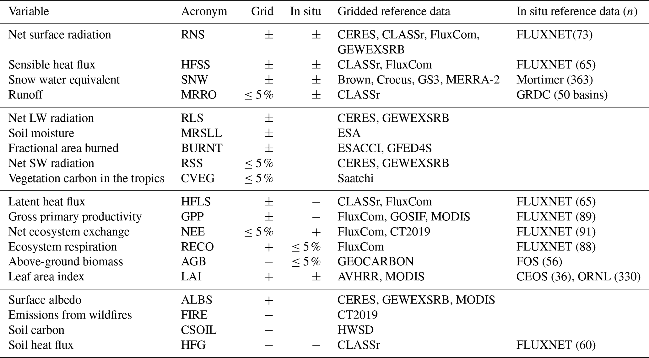
We start our evaluation with a qualitative overview of how the choice of meteorological forcing (CRUJRAv2, GSWP3W5E5, CRUNCEP) and reference data affect global mean biases. Our results show that for 10 out of 19 variables assessed in this study, the sign of the bias changes depending on what forcing and reference data are used (Table 2). Assuming that global values are reasonably accurate if (i) the sign of the bias varies depending on the choice of forcing and/or reference, or (ii) the global mean bias is reasonably small (≤5 %), we can divide our variables into four groups. The first group includes variables that show accurate global mean values for both gridded and in situ reference data. This includes the following variables: net surface radiation, sensible heat flux, snow water equivalent, and runoff (Table 2). The second group consists of variables that lack in situ observations but show accurate values when assessed against gridded reference data. This involves the following variables: net LW radiation, soil moisture, fractional area burned, net SW radiation, and vegetation carbon in the tropics. The third group includes variables that show accurate values for either globally gridded data (latent heat flux, GPP, NEE) or in situ reference data (ecosystem respiration, above-ground biomass, and LAI). For this group of variables, it will be important to assess the differences between evaluations based on gridded and in situ data in more detail. The fourth group includes variables with systematic biases across all evaluations, which includes surface albedo, emissions from wildfires, soil carbon, and soil heat flux. The following sections evaluate biases and other statistical metrics for each variable in detail.

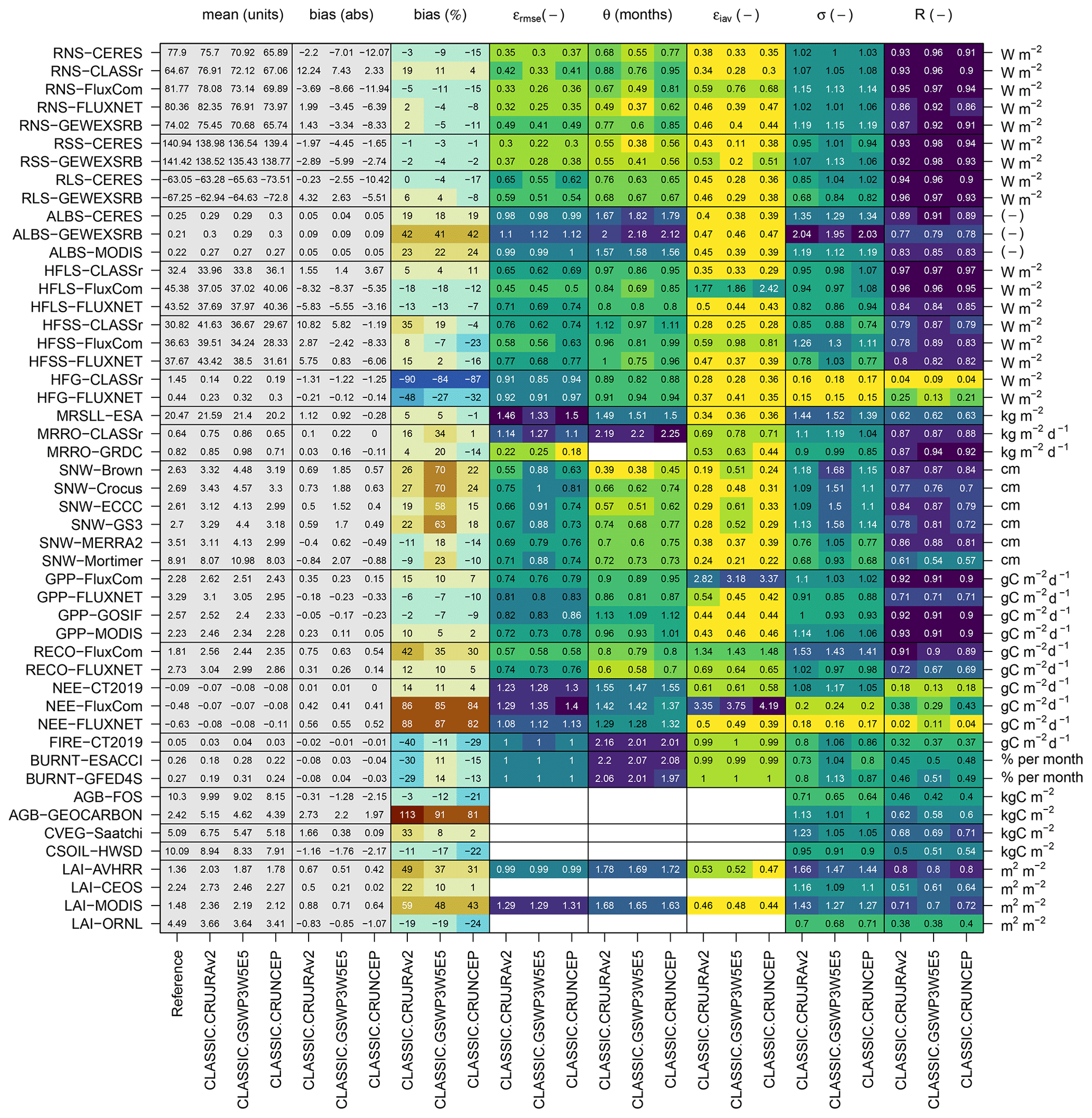
Figure 5 Global mean values of statistical metrics defined in Sect. 2. The color ranges span the minimum and maximum for each metric. The physical units of the mean and absolute bias are given by the vertical axis on the right-hand side.

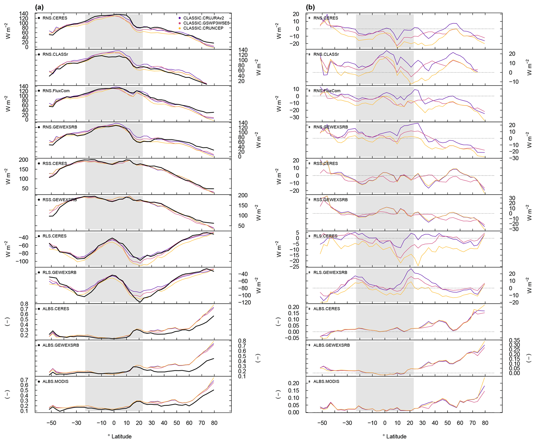
Figure 6 (a) Zonal mean values and (b) corresponding biases for variables related to the radiation cycle.

3.1 Net surface radiation

RNS biases range from positive to negative values, depending on the choice of forcing (CRUJRAv2, GSWP3W5E5, CRUNCEP) and reference data (CERES, CLASSr, FluxCom, GEWEXSRB, and FLUXNET). For instance, global mean biases range from −15 % (−12.07 W m⁻²) when forcing CLASSIC with CRUNCEP and evaluating results against CERES (2000–2012), to +19 % (+12.24 W m⁻²) for CRUJRAv2 and CLASSr (2003–2009) (Fig. 5). Evaluating model output against in situ measurements by FLUXNET yields mean biases that range from −8 % (−6.39 W m⁻² for CRUNCEP) to +2 % (+1.99 W m⁻² for CRUJRAv2) (Figs. 5 and 1a).

Zonal mean values in net surface radiation are in close agreement with the corresponding reference values, with biases that range from −20 to +20 W m⁻² (Fig. 6). The same figure shows that net surface radiation biases in the NH extratropics are negative when evaluating CLASSIC against CERES, FluxCom, and GEWEXSRB, and positive when choosing CLASSr as a reference data set. Considering all three model runs and four gridded reference data sets shows that for most grid cells annual mean biases can be both negative and positive, depending on which model run is compared against which reference data (Fig. 7a). The strongest annual mean bias is located in the Tibetan Plateau with values below −30 W m⁻². Hovmöller diagrams show that CLASSIC captures the observed seasonality well across all latitudes (Fig. 8). Monthly biases range from negative to positive values across most latitudes and months, depending on the choice of meteorological forcing and reference data. This suggests that model values are reasonably accurate across space and time when considering the uncertainties associated with the forcing and all four globally gridded reference data.

Other statistical metrics confirm that CLASSIC reproduces net surface radiation reasonably well. The relative measure of the centralized root-mean-square error (ε_crmse) ranges from 0.30 to 0.49 (unitless), which is lower than for most other variables (Fig. 5). Differences in the timing of modeled and observed seasonal peaks (θ) are less than 1 month. Modeled interannual variability is lower compared to CERES, CLASSr, GEWEXSRB, and FLUXNET, and larger than FluxCom (not shown). The relative interannual variability error (ε_iav) is reasonably small (0.30 to 0.76, unitless). CLASSIC reproduces the spatial variability of annual mean values well, where the ratio of model and reference standard deviation in space (σ) is close to unity (1.00 to 1.19). Also, the spatial correlation coefficients (R) range from 0.86 to 0.97. Averaging the resulting scores across all three ensemble members shows that S_overall ranges from 0.74 to 0.80 (unitless), depending on the reference data (Fig. 9a). The choice of meteorological forcing affects scores by less than 0.1 (Fig. 9b). Scores tend to be higher when forcing CLASSIC with GSWP3W5E5 (Fig. 9c).

3.2 Net shortwave and longwave radiation

Results for net SW radiation (RSS) and LW radiation (RLS) are mainly consistent with findings for net surface radiation described above. Net SW and LW radiation values produced by CLASSIC are reasonably accurate when considering uncertainties associated with meteorological forcing and reference data (CERES and GEWEXSRB). Global mean biases for net SW radiation range from −1 % (−1.65 W m⁻²) to −4 % (−5.99 W m⁻²) (Fig. 5). For net LW radiation, global mean biases range from −17 % (−10.42 W m⁻²) to +6 % (+4.32 W m⁻²). CLASSIC captures the zonal mean values and seasonal patterns of both variables well (Figs. 6, A4, and A5). However, CLASSIC also shows a systematic negative SW radiation bias in the NH extratropics from December to May (up to −40 W m⁻²) (Fig. A4), which is consistent with a surface albedo bias as discussed further below. Results for other statistical metrics and corresponding scores are similar to the ones described for net surface radiation. For net SW radiation, ε_crmse range between 0.22 and 0.38 (unitless), θ ranges from 0.38 to 0.56 months, ε_iav ranges from 0.11 to 0.53 (unitless), σ ranges from 0.94 to 1.13 (unitless), and R ranges from 0.92 to 0.98 (Fig. 5). For net LW radiation, values in ε_crmse and θ are considerably higher than for net SW radiation, where ε_crmse ranges from 0.51 to 0.65 (unitless) and θ ranges from 0.63 to 0.76 months. The overall scores are higher for net SW radiation (S_overall≈0.80) than for net LW radiation (S_overall=0.72) (Fig. 9). The choice of the forcing has a considerable impact on how well the model captures the interannual variability of both net SW and LW radiation. The difference between the maximum and minimum interannual variability scores (S_iav) ranges from 0.10 to 0.21, depending on the reference data (Fig. 9b). For net LW radiation, the choice of the forcing has also a considerable impact on the bias score (ΔS_bias: 0.17–0.2). CLASSIC performs best when forcing the model with GSWP3W5E5 (Fig. 9c).

Figure 7 Model ensemble mean values and respective biases for (a) net surface radiation and (b) surface albedo. The mean, minimum, and maximum ensemble biases refer to the mean, minimum, and maximum values across all evaluations, respectively. For instance, a minimum bias that is negative implies that at least one evaluation yields a negative bias.

3.3 Albedo

Surface albedo (ALBS) shows a positive global mean bias across all three ensemble members and reference data sets (CERES, GEWEXSRB, and MODIS), ranging from +18 % to +42 % (+0.04 to +0.09, unitless) (Fig. 5). This bias occurs mainly in the NH extratropics, with increasing values towards higher latitudes (+0.2; Figs. 6 and 7b). The strongest annual mean bias is located in the Tibetan Plateau with values above 0.3. In the NH extratropics, the bias is most evident during the cold season (+0.4 between 60 and 80^∘ N from December to January) (Fig. A6). Larger biases (+0.5) are present north of 80^∘ N, but this involves only few grid cells. The timing of the bias suggests a possible relation with snow and/or the large solar zenith angle. The performance with respect to other statistical metrics tends to be lower than for net SW radiation. Values for ε_crmse range between 0.98 and 1.12 (unitless), θ ranges from 1.67 to 2.18 months, ε_iav ranges from 0.38 to 0.48 (unitless), σ ranges from 1.12 to 2.04 (unitless), and R ranges from 0.77 to 0.91 (Fig. 5). The corresponding overall score S_overall ranges between 0.48 and 0.59, depending on the reference data (Fig. 9). The S_overall values are not very sensitive to the choice of forcing (ΔS_overall=0.01).

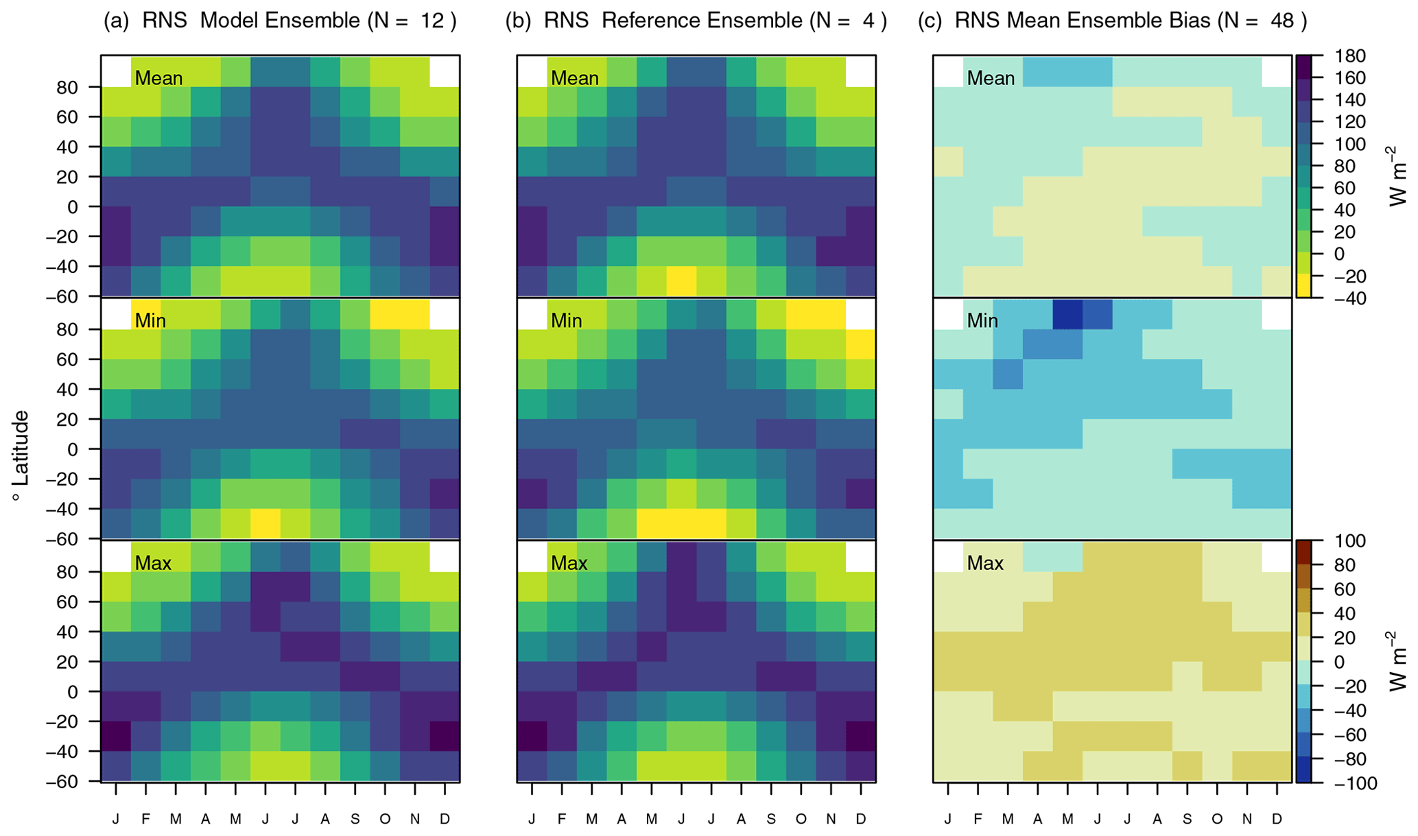
Figure 8 Net surface radiation computed from three model runs (CLASSIC driven with CRUJRAv2, GSWP3W5E5, and CRUNCEP) and four reference data sets (CERES, CLASSr, FluxCom, and GEWEXSRB). The top, center, and bottom rows provide ensemble mean, minimum, and maximum values for (a) CLASSIC, (b) reference data, and (c) corresponding biases. The mean, minimum, and maximum ensemble biases refer to the mean, minimum, and maximum values across all evaluations, respectively. For instance, a minimum bias that is negative implies that at least one evaluation yields a negative bias.

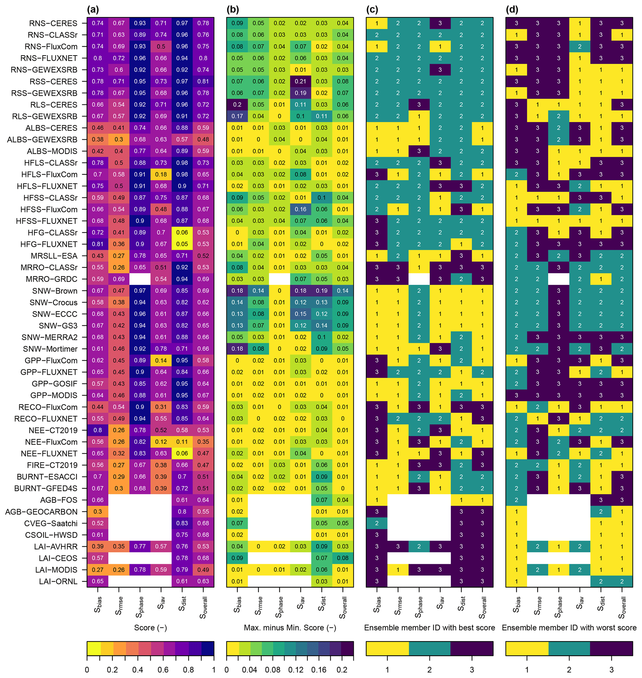
Figure 9 (a) Mean ensemble score, (b) maximum score difference among ensemble members, and ensemble member with the (c) highest and (d) lowest score. Ensemble member IDs refer to model runs conducted with data from (1) CRUJRAv2, (2) GSWP3W5E5, and (3) CRUNCEP.

3.4 Heat fluxes

CLASSIC reproduces the partitioning of net surface radiation into sensible (HFSS), latent (HFLS), and soil heat flux (HFG) reasonably well. Global mean values in sensible heat flux simulated by CLASSIC are likely to be reasonable, with biases that range from negative to positive values, depending on the meteorological forcing (−23 % to +35 %, −8.33 to +10.82 W m⁻²) (Figs. 5 and 10). Driving CLASSIC with CRUNCEP causes biases to be negative for all three reference data sets, while the opposite is true when running the model with CRUJRAv2. For latent heat flux, the sign of the bias is consistent across all ensemble members, with negative biases when compared against FluxCom (−12 % to −18 %, −5.35 to −8.32 W m⁻²) and FLUXNET (−7 % to −13 %, −3.16 to −5.83 W m⁻²) and reasonably small positive biases when evaluated against CLASSr (+5 % to +11 %, +1.55 to +3.67 W m⁻²). Biases in soil heat flux are negative across all ensemble members and both reference data sets (CLASSr and FLUXNET) (−32 % to −90 %). However, it must be noted that the corresponding absolute values are small (−0.14 to −1.31 W m⁻²), implying that the impact of annual mean soil heat flux biases on the surface energy balance is minor. The relative partitioning of net surface radiation into sensible and latent heat fluxes is well reproduced, with reasonably small positive and negative biases, depending on the meteorological forcing (Fig. 10b). A more detailed assessment of each heat flux is provided next.

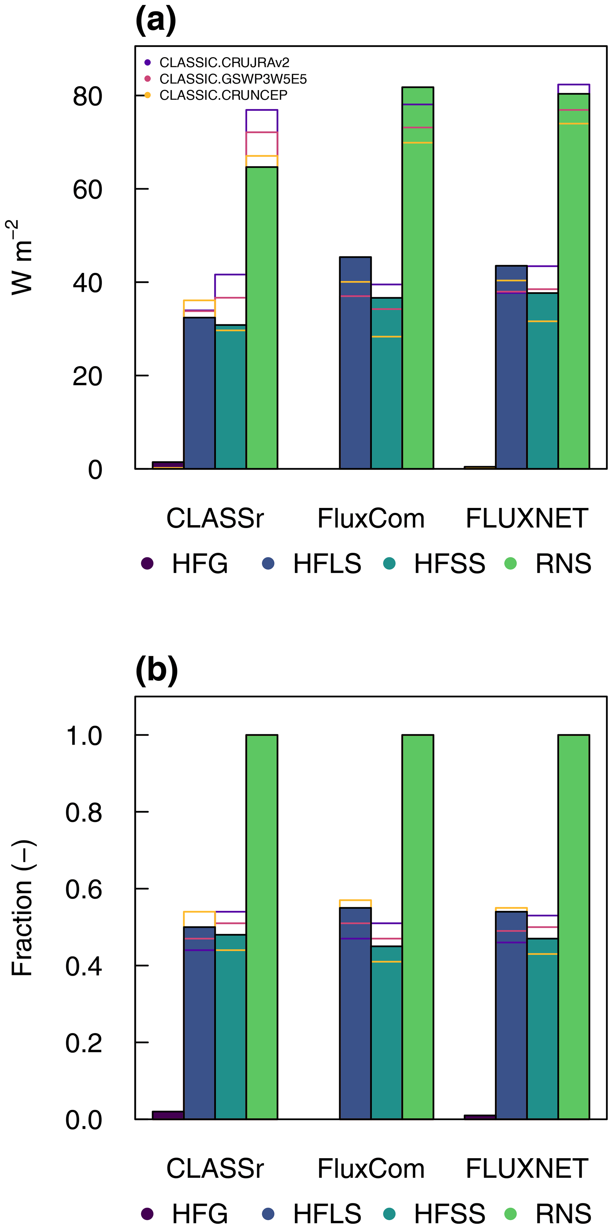
Figure 10 (a) Annual mean values of soil heat flux (HFG), latent heat flux (HFLS), sensible heat flux (HFSS), and net surface radiation (RNS) for the three CLASSIC ensemble members and for the reference data (CLASSr, FluxCom, and FLUXNET). Panel (b) shows the corresponding fractions with respect to net surface radiation.

CLASSIC reproduces the zonal mean patterns of sensible and latent heat flux well, with zonal mean biases of about ±20 W m⁻² (Fig. 11). For sensible heat flux, zonal mean biases range from positive to negative values across all latitudes, depending on the meteorological forcing (Figs. 11 and A7a). For latent heat flux, biases are primarily positive when compared against CLASSr and negative for FluxCom, regardless of the forcing (Figs. 11 and A7b). Zonal mean patterns of soil heat flux data from CLASSr are not well captured, with biases that become increasingly negative towards higher latitudes (−4 W m⁻² in the Arctic) (Figs. 11 and A8a).

CLASSIC captures the seasonal cycle of all three heat fluxes reasonably well (Figs. A9, A10, and A11). The negative latent heat flux biases are stronger during the warm season in both hemispheres. For soil heat fluxes, CLASSIC tends towards a more intense seasonal cycle in the extratropics, with positive biases in the warm and negative biases in the cold season.

Values of ε_rmse are similar among sensible and latent heat flux (0.45 to 0.77, unitless) and higher for soil heat flux (0.85 to 0.97) (Fig. 5). For all three heat fluxes, time lags in seasonal peaks are close to 1 month. The interannual variability of sensible and latent heat fluxes tends to be smaller compared to the CLASSr reference data set and larger compared to FluxCom (not shown), implying that model values lie within the uncertainty of the reference data. The corresponding ε_iav values range from 0.25 to 2.42 (unitless), where the higher values are obtained when evaluating CLASSIC against FluxCom (Fig. 5). For soil heat flux, modeled interannual variability is very similar to the corresponding reference values (not shown), leading to low values of ε_iav (0.28 to 0.36). Values of σ and R are reasonable for sensible heat flux (σ: 0.74 to 1.26, R: 0.78 to 0.89) and latent heat flux (σ: 0.94 to 1.08, R: 0.84 to 0.97), and poor for soil heat flux (σ: 0.15 to 0.17, R: 0.04 to 0.21). Consistently, the corresponding S_overall values are higher for latent and sensible heat flux (0.64 to 0.73) and lower for soil heat flux (0.53) (Fig. 9). From all three heat fluxes, sensible heat flux is most sensitive to the choice of forcing, with ΔS_overall equal to 0.04 when driving the model with GSWP3W5E5.

3.5 Soil moisture

Global mean values in soil moisture (MRSLL) of the top 10 cm are very close to the corresponding reference values from ESA (1979–2017), with biases ranging from −1 % (−0.28 kg m⁻², CRUNCEP) to +5 % (about +1 kg m⁻², CRUJRAv2 and GSWP3W5E5) (Fig. 5). Zonal mean values are well reproduced with a tendency towards a positive bias north of 60^∘ N (+10 kg m⁻²) (Fig. 11). This bias is caused by clusters of grid cells located in different parts of the Arctic (Fig. A8b). The positive bias is present in all ensemble members and occurs from June to September (Fig. A12). Other statistical metrics confirm that the performance does not differ largely among ensemble members (Fig. 9). Values of ε_rmse and time lags of seasonal peaks (θ) are higher compared to most other variables (ε_rmse≤1.5, θ≈1.5 months). The spatial variability is larger than in the reference data (σ≈1.44, unitless) and correlation coefficients are relatively low (R≈0.62). The corresponding overall score is 0.52 and is not very sensitive to the choice of forcing (ΔS_overall=0.01) (Fig. 9).

3.6 Runoff and streamflow

Global mean runoff (MRRO) biases range from +1 % (< 0.005 kg m⁻² d⁻¹, CRUNCEP) to +34 % (0.22 kg m⁻² d⁻¹, GSWP3W5E5) when evaluated against CLASSr (2003–2009) (Fig. 5). This difference is consistent with the higher precipitation values found for the GSWP3W5E5 forcing. CLASSIC reproduces the zonal mean pattern of gridded reference runoff from CLASSr well, with mainly positive biases when forcing CLASSIC with GSWP3W5E5 (Fig. 11). Smaller, including negative, zonal mean biases occur when forcing CLASSIC with CRUNCEP. Consistently, the sign of the bias varies for many grid cells depending on the forcing (Fig. A13a). Furthermore, the sign of the bias varies for most latitudes and months (Fig. A14), suggesting that modeled runoff is within the uncertainty range of the meteorological forcing. CLASSIC reproduces the spatial patterns of runoff reasonably well, with σ values between 1.04 and 1.14 and R values between 0.87 and 0.88 (Fig. 5). The timing of the seasonal peaks, however, differs by more than 2 months, and ε_rmse values exceed 1 when using CLASSr as reference data. The overall score averaged over the three ensemble members is 0.53, with a better score when driving CLASSIC with CRUNCEP and worse when using GSWP3W5E5 as a forcing data set (Fig. 9).

Summing up the annual runoff from all grid cells located within each of the world's 50 largest river basins and comparing those values against annual mean streamflow at the corresponding river mouths yields biases that range between −14 % (−0.11 kg m⁻² d⁻¹, CRUNCEP, GRDC) to +20 % (+0.16 kg m⁻² d⁻¹, GSWP3W5E5, GRDC). For most basins, the sign of the bias remains constant regardless of the forcing (Fig. 1e for CRUJRAv2 as an example). CLASSIC reproduces the spatial patterns of streamflow reasonably well, with σ values close to 1 and R values ranging between 0.87 and 0.92 (Fig. 5). The overall score averaged over the three ensemble members is 0.69. Performance is better when driving CLASSIC with CRUNCEP and worse when using GSWP3W5E5 as a forcing data set (Fig. 9).

3.7 Snow water equivalent

Global mean SNW biases range from −14 % (−0.49 cm, CRUNCEP-driven run evaluated against MERRA-2) to +70 % (+1.88 cm, GSWP3W5E5-driven run evaluated against Crocus) for the 1981–2017 period (Fig. 5). Evaluating CLASSIC against in situ measurements compiled by Mortimer et al. (2020) shows that the mean bias can be negative (−10 %, −0.88 cm, CRUNCEP) or positive (+23 %, +2.07 cm, GSWP3W5E5), depending on the forcing (Figs. 5 and 1f). The higher snow water equivalent values in GSWP3W5E5-driven results are consistent with the higher precipitation values found for this forcing. For most evaluations, CLASSIC reproduces zonal mean values well when driven with CRUJRAv2 or CRUNCEP (Fig. 11). The sign of the bias ranges from positive to negative for most grid cells (Fig. A13b). Positive biases tend to be larger in eastern Canada, northern Scandinavia, and northern Siberia, and during NH spring (Fig. A15b).

Other statistical metrics confirm that CLASSIC's ability to reproduce snow water equivalent tends to be weaker when driven with GSWP3W5E5 (ε_rmse: 0.55 to 0.91, θ: 0.38 to 0.77, ε_iav: 0.19 to 0.61, σ: 0.68 to 1.68, and R: 0.54 to 0.87) (Fig. 5). The corresponding S_overall values range from 0.62 to 0.69, with lower scores when driving CLASSIC with GSWP3W5E5 and higher scores when using CRUJRAv2 (Fig. 9). Site-level-based score values are similar to grid-level score values, with an overall score of 0.66.

Table 3 Globally summed mean values and corresponding biases.

3.8 Gross primary productivity

Globally accumulated annual mean values of GPP computed from different reference data are of similar magnitude, with 115 Pg C yr⁻¹ for FluxCom (1980–2013), 121 Pg C yr⁻¹ for MODIS (2000–2016), and 130 Pg C yr⁻¹ for GOSIF (2000–2017) (Table 3). The corresponding model biases are reasonably small, with negative values when comparing CLASSIC against GOSIF (−2 % to −10 %), and positive values when evaluating against MODIS ($<+\mathrm{1}$ % to +10 %) or FluxCom (+4 % to +14 %). An assessment with eddy covariance data shows that biases range from −6 % to −10 % (Fig. 5). CLASSIC captures zonal mean GPP patterns well with no systematic bias pattern among evaluations (Fig. 12). Annual mean biases range from negative to positive for most grid cells, depending on the forcing and reference data (Fig. A16a). Hovmöller diagrams show that CLASSIC captures the seasonal GPP cycle well across all latitudes, with no systematic biases (Fig. A17). A more regional assessment, however, shows that the seasonal GPP cycle is out of phase in parts of the humid tropics of South America and Africa (not shown). Values in ε_rmse are less than 1 for all evaluations, and time lags of seasonal peaks are about 1 month on average (Fig. 5). CLASSIC reproduces the interannual variability of GPP well when compared against FLUXNET, GOSIF, and MODIS (ε_iav<0.6). Higher ε_iav values are found when evaluating the model against FluxCom. However, it must be noted that interannual variability patterns from FluxCom are not reliable (Jung et al., 2020). Spatial patterns of GPP are well captured, with values of σ close to 1 and correlation coefficients around 0.91. The corresponding overall scores range from 0.58 (FluxCom) to 0.67 (MODIS), with higher scores when forcing CLASSIC with CRUJRAv2 (Fig. 9).

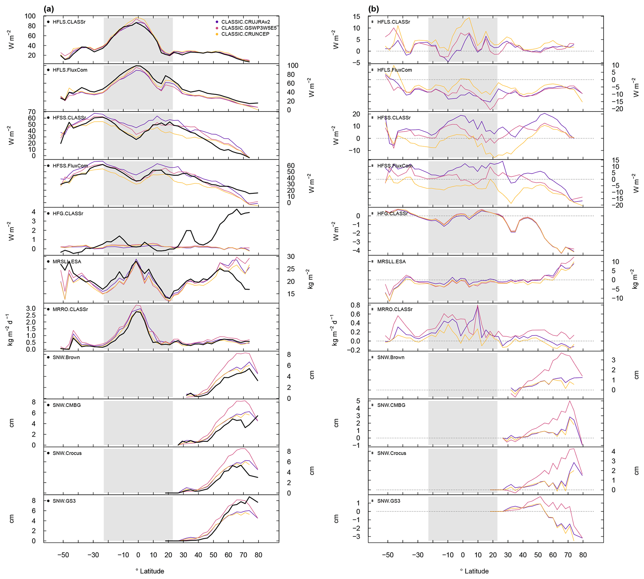
Figure 11 (a) Zonal mean values and (b) corresponding biases for heat fluxes and variables related to the water cycle.

3.9 Ecosystem respiration

Annual mean biases of RECO are reasonably small across FLUXNET sites, with mean biases ranging from +5 % to +12 %, depending on the forcing (Fig. 5). Looking at the spatial distribution of FLUXNET sites suggests that the positive biases are more evident in the NH extratropics rather than in the tropics (Fig. 2b). Larger biases are present when comparing CLASSIC with FluxCom; however, those values are not reliable as FluxCom underestimates ecosystem respiration in the tropics (Jung et al., 2020). Other statistical metrics derived from FLUXNET data suggest that CLASSIC reproduces ecosystem respiration reasonably well (ε_rmse≈0.75, θ<1, ε_iav≈0.66, σ≈1.0, R≈0.69) (Fig. 5). The corresponding overall score is 0.64 (Fig. 9). This score value is insensitive to the choice of forcing.

3.10 Net ecosystem exchange

Globally accumulated annual mean NEE computed from CT2019 is −4.2 Pg C yr⁻¹ for the period 2000–2016 (Table 3). The corresponding value from FluxCom is −24.9 Pg C yr⁻¹ for the period 1980–2013, which is unrealistic and due to an underestimation of ecosystem respiration in the tropics (Jung et al., 2020). CLASSIC's estimate of annual mean NEE ranges from −4.2 to −4.6 Pg C yr⁻¹ (2000–2016), which corresponds to a bias of about −1 % to −10 % when compared against CT2019, depending on the meteorological forcing. However, much larger biases apply when evaluating CLASSIC against FLUXNET (+88 %; Figs. 2c and 5).

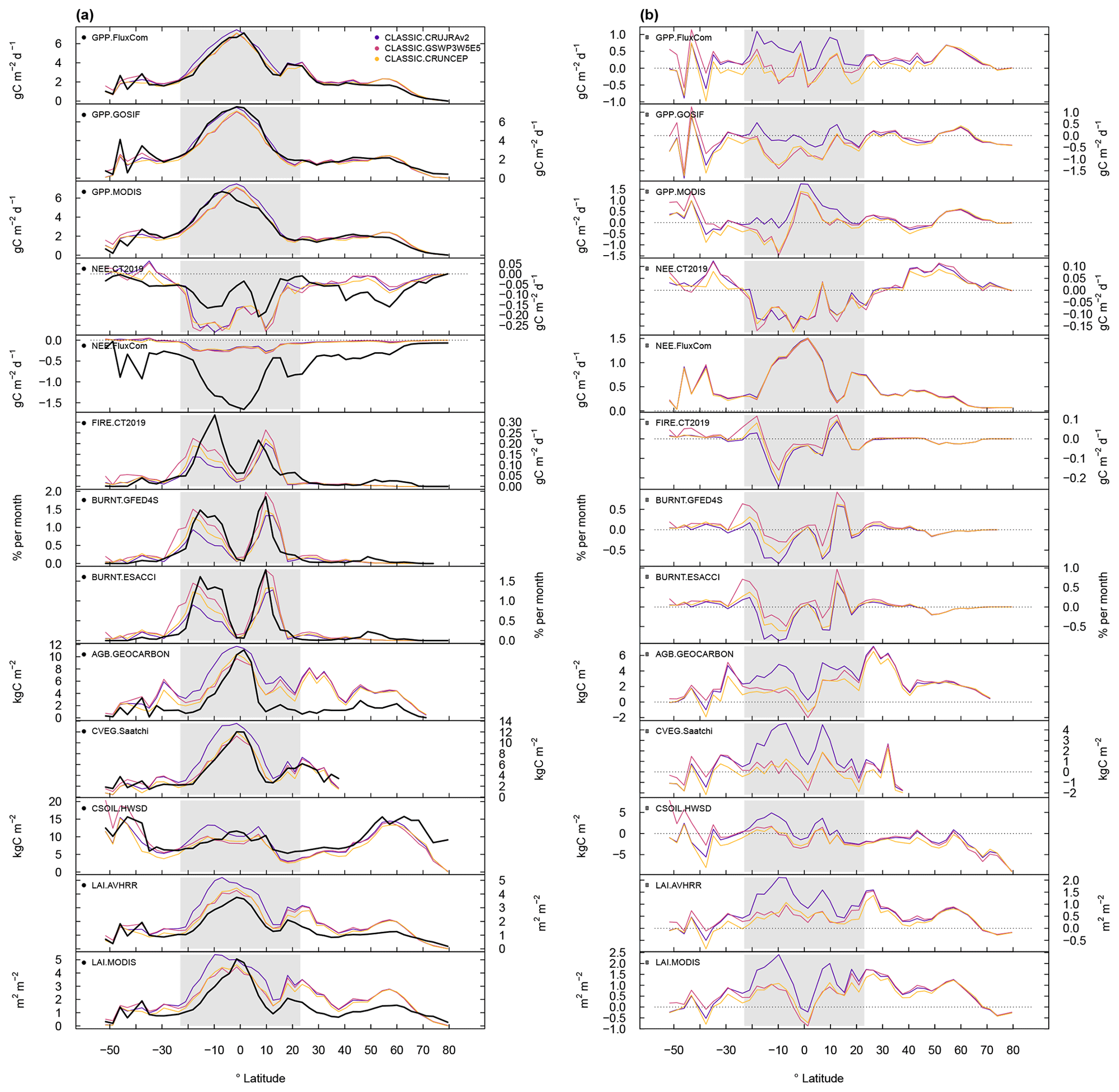
Figure 12 (a) Zonal mean values and (b) corresponding biases for variables related to the carbon cycle.

Zonal mean NEE patterns resemble values from CT2019 to a certain degree (Fig. 12). The strength of the carbon sink is modeled to be stronger in the tropics (−0.15 g C m⁻² d⁻¹) and weaker in the extratropics (+0.10 g C m⁻² d⁻¹) compared to CT2019. FLUXNET data confirm the tendency towards a positive bias, i.e. weaker sink, in the NH extratropics (Fig. 2c). In the tropics, however, the sign of the bias is mixed, and the number of sites is too small to confirm whether or not CLASSIC overestimates the strength of the carbon sink at low latitudes.

Hovmöller diagrams suggest that CLASSIC reproduces the general pattern of the seasonal NEE cycle in the extratropics, where the strength of the carbon sink is strongest during the warm period (Fig. A18). Other statistical metrics suggest a considerable mismatch between model and reference NEE (ε_rmse>1, θ>1, and R<0.2). The corresponding overall scores are 0.47 for FLUXNET and 0.53 for CT2019 (Fig. 9).

3.11 Area burned and resulting emissions

Wildfires are estimated to burn an area of about 4.6× 10⁶ km² yr⁻¹ (ESACCI from 2001–2017 and GFED4S from 2001–2015), causing emissions of about 2.9 Pg C yr⁻¹ (CT2019, 2000–2017) (Table 3, where BURNT refers to area burned and FIRE refers to the associated emissions). CLASSIC reproduces the spatial extent of wildfires well considering the uncertainty of the meteorological forcing, with biases ranging from −28 % when forcing CLASSIC with CRUJRAv2, to +14 % for GSWP3W5E5. The higher fractional area burned values in GSWP3W5E5 are not related to precipitation, as GSWP3W5E5 is the wettest of the three forcing data sets across all latitudes and seasons. Instead, GSWP3W5E5 has larger values in near-surface wind speeds compared to the other forcing data sets, which increase the probability of wildfires. Model values for emissions from wildfires tend to be lower than observed, with biases ranging from −37 % (CRUJRAv2) to −7 % (GSWP3W5E5).

CLASSIC reproduces the zonal mean pattern of both variables well, with values that are highest at 10^∘ S and 10^∘ N (Fig. 12). The sign of the zonal mean bias is consistent between both variables. Biases tend to be negative in the humid parts of the tropics and positive in the drier parts of the tropics (Figs. 12 and A19). CLASSIC reproduces the seasonality of both variables well, with lower values when the solar zenith angle in the tropics is small (Figs. A20 and A21), which is indicative of the position of the intertropical convergence zone. While biases are most evident in the tropics, the model also underestimates fractional area burned and associated emissions in the boreal forests. Other statistical metrics suggest that considerable differences between model and reference values remain (ε_rmse=1.0, θ>2 months, ε_iav≈1, and R≤0.51) (Fig. 5). The resulting overall scores for fractional area burned and emissions from fires are 0.51 and 0.47, respectively (Fig. 9). These score values are not very sensitive to the choice of forcing (ΔS_overall≤0.01).

3.12 Vegetation biomass

Reference values from GEOCARBON estimate globally accumulated AGB with 214.5 Pg C. The corresponding values from CLASSIC range from 364.9 Pg C (+70 %) to 442.3 Pg C (+106 %) (Table 3). The bias is largest between 20^∘ N and 40^∘ N, in particular in the eastern US and in East Asia (Figs. 12 and A22a). Comparing CLASSIC against vegetation carbon (i.e. above- and below-ground living biomass; CVEG) for the tropics provided by Saatchi et al. (2011) suggests smaller biases (+2 % for CRUNCEP to +33 % for CRUJRAv2) (Figs. 5, 12, and A22b). Spatial correlations are weak, with R≤0.62 for above-ground biomass and R≤0.71 for vegetation carbon (Fig. 5). The corresponding overall scores are 0.55 (ΔS_overall=0.01) for above-ground biomass and 0.68 (ΔS_overall=0.05) for vegetation carbon in the tropics (Fig. 9).

To investigate differences between CLASSIC and GEOCARBON in greater detail, we evaluate model and reference above-ground biomass values against forest inventory data (FOS). The comparison shows a larger negative bias for GEOCARBON (−50 %) and a smaller negative bias for CLASSIC (−3 % for CRUJRAv2 to −21 % for CRUNCEP) (Figs. 5 and 2d). This finding suggests that GEOCARBON may be subject to considerable uncertainties, which may contribute to the large bias when evaluating CLASSIC against GEOCARBON. More forest inventory data are required to reach a conclusive result, as the current spatial coverage of inventory plots provided by FOS is modest. Evaluating CLASSIC against FOS yields an overall score of 0.64 (Fig. 9).

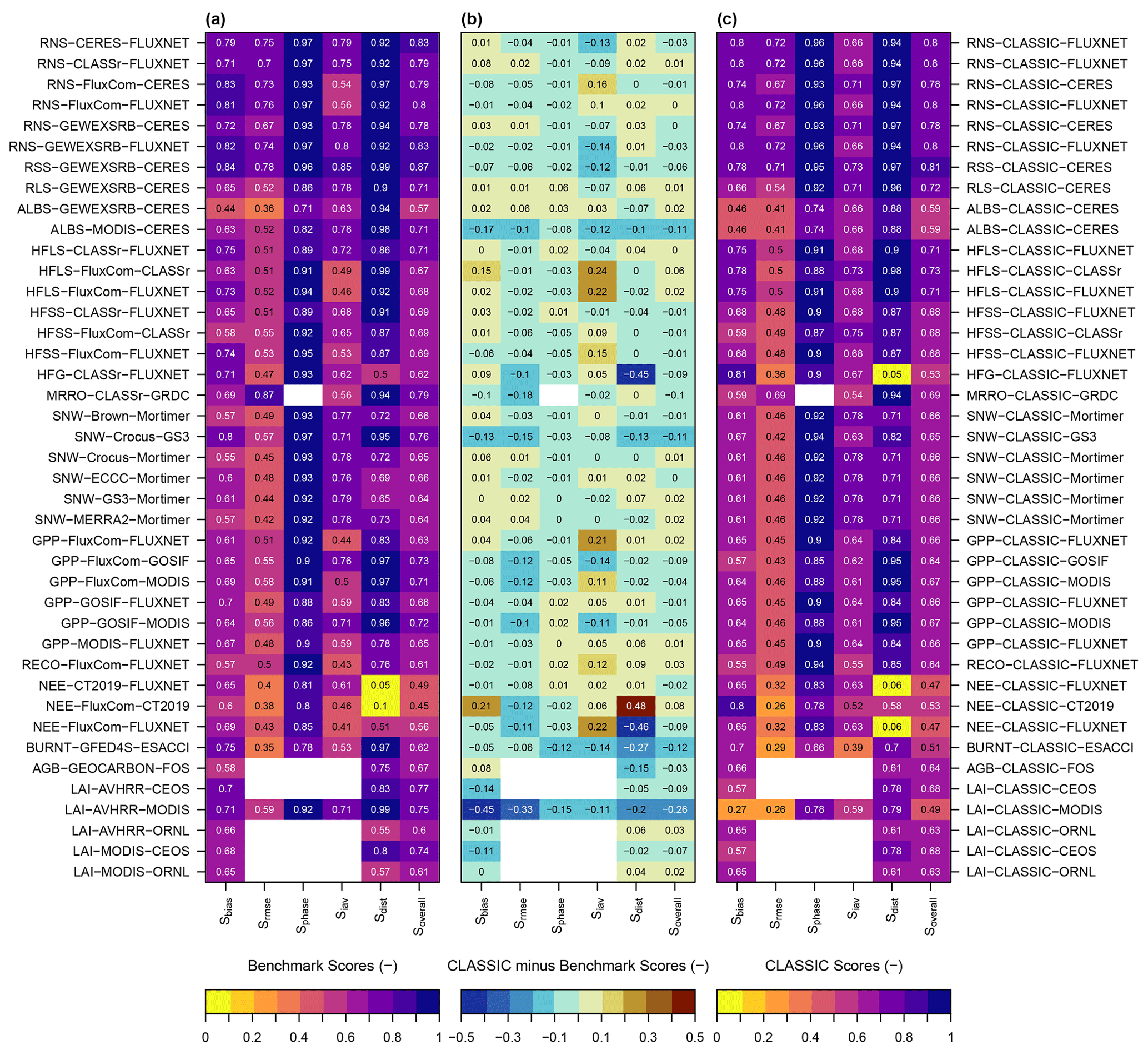
Figure 13 (a) Benchmark scores computed from reference data only, (c) mean model ensemble skill scores, and (b) corresponding score difference.

3.13 Soil carbon

The global stock of soil carbon (CSOIL) is estimated with 1198 Pg C (HWSD). The corresponding values from CLASSIC range from about 956 Pg C (−20 %; CRUNCEP) to 1109 Pg C (−8 %; CRUJRAv2) (Table 3). CLASSIC reproduces the zonal mean patterns of soil carbon well, with a tendency for negative biases in the Arctic (−10 kg C m⁻²) (Fig. 12). Some of this bias is related to a small number of grid cells at high latitudes with particularly large biases (−40 kg C m⁻²) (Fig. A23a). The higher values in the reference data may be related to the presence of permafrost and peatland, which are currently not represented in CLASSIC. The spatial variability of soil carbon is well reproduced (σ≈0.92), but the spatial correlation is rather weak (R≈0.5) (Fig. 5). The corresponding overall score is 0.68 (ΔS_overall=0.01) (Fig. 9).

3.14 Leaf area index

Evaluating CLASSIC with gridded LAI data from AVHRR (1982–2010) and MODIS (2000–2009) suggests large positive global mean biases that range from +31 % (+0.42 m⁻² m⁻²) to +59 % (+0.88 m⁻² m⁻²), depending on the forcing and reference data (Fig. 5). While CLASSIC reproduces the general pattern of zonal mean LAI reasonably well, the model has a positive bias across most latitudes (Fig. 12). However, biases have a local minimum at the Equator, especially when using MODIS as a reference. All six evaluations tend towards positive biases in forested regions of the NH extratropics and the drier parts of the tropics (Fig. A23b). In the more humid tropics of the Amazon and Congo basin, biases range from negative to positive values, depending on the forcing and reference data. Hovmöller diagrams show that the positive bias in the NH extratropics occurs mainly during the cold season, suggesting a possible relation with snow, leaf shedding, and/or the larger solar zenith angle (Fig. A24). For most of the remaining months and latitudes, LAI biases range from positive to negative biases, suggesting that modeled values are reasonably accurate when considering the uncertainty of the meteorological forcing and reference data.

Other statistical metrics suggest further differences between model and reference LAI. Values of ε_rmse are higher than for most other variables (0.99 to 1.31), and time lags in seasonal peaks range between 1 and 2 months (Fig. 5). The spatial variability of LAI is considerably larger for model data than gridded reference data (σ ranges from 1.27 to 1.66), and the correlation coefficients are reasonable but not impressive (0.7 to 0.8). The corresponding overall scores are 0.49 (ΔS_overall=0.01) and 0.53 (ΔS_overall=0.03) when evaluating CLASSIC against gridded LAI reference data from MODIS and AVHRR, respectively (Fig. 9).

To investigate the apparent LAI bias further, we evaluate model and reference LAI values with in situ measurements of maximum LAI provided by ORNL. The comparisons show larger negative biases for MODIS (−37 %) and AVHRR (−33 %), and smaller negative biases for CLASSIC (−19 % to −24 %) (Figs. 5 and 2f for CLASSIC only). This suggests that (i) it is unlikely that CLASSIC overestimates maximum LAI, and (ii) the large positive LAI bias discussed above may in part be due to an underestimation of LAI by the gridded reference data set. Furthermore, evaluating CLASSIC against in situ LAI observations from CEOS shows mean biases that range from +1 % to +22 % (Figs. 5 and 2e). The corresponding values for MODIS and AVHRR are −6 % and −4 %, respectively (not shown). Given these findings, we conclude that the large positive LAI found for CLASSIC when evaluated against AVHRR and MODIS must be interpreted with caution. One possible reason for lower LAI in satellite-based reference data at high latitudes is the problems associated with LAI retrievals during winter months when the sun is low and the surface is snow covered.

3.15 Benchmark scores derived from reference data only

Benchmark scores are produced by comparing two independent reference data sets (Fig. 3). This exercise fulfills three purposes. First, benchmark scores quantify observational uncertainty, where lower values imply larger uncertainties. Second, we can evaluate the quality of gridded products using in situ measurements. Third, comparing model scores against benchmark scores shows how well CLASSIC performs relative to the performance of a reference data set. The comparison of two reference data sets is limited to the time period for which both data sets overlap.

Our results demonstrate that most benchmarks are considerably low, suggesting that observational uncertainties are large. For most variables, model skill scores are very similar to benchmark skill scores, implying that CLASSIC performs similarly to a reference data set. In some cases, CLASSIC even outperforms gridded reference data sets when evaluating gridded reference data and model output against in situ measurements. The remaining section discusses these findings in more detail.

Contrary to our expectations, most benchmark scores are far below unity (Fig. 13). Only two variables show S_overall values equal to or greater than 0.8 (net surface radiation and net SW radiation). The largest uncertainties are found for NEE, with S_overall=0.49 when comparing CT2019 against FLUXNET. Even lower score values are found when evaluating FluxCom NEE against FLUXNET due to the known limitations of the FluxCom data set discussed in Sect. 2.4.2.

Comparing gridded reference data against in situ measurements shows subtle differences in how well gridded products perform for the same variable. For net surface radiation, S_overall values range from 0.79 for CLASSr to 0.83 for CERES when evaluated against FLUXNET. For latent heat flux, CLASSr (S_overall=0.71) performs slightly better than FluxCom (S_overall=0.68). For sensible heat flux, CLASSr and FluxCom perform equally well (S_overall=0.69). For snow water equivalent, the blended multi-reference mean data (ECCC; S_overall=0.66) perform very similarly to the individual reference data (S_overall: 0.64 to 0.66) when evaluated against in situ measurements provided by Mortimer et al. (2020). For GPP, the S_overall values are highest for GOSIF (0.66), followed by MODIS (0.65) and FluxCom (0.63) when evaluated against FLUXNET. In the case of NEE, S_overall values are higher for FluxCom (0.56) than for CT2019 (0.49). However, it must be noted that the majority of FLUXNET sites are located in the NH extratropics, implying that corresponding scores reflect the performance in primarily non-tropical regions. For LAI, the S_overall values are 0.61 for MODIS and 0.60 for AVHRR when evaluated against in situ measurements from ORNL and 0.74 (MODIS) and 0.77 (AVHRR) when compared against data from CEOS.

In most cases, model skill score values are very similar to the corresponding benchmark score values. For instance, evaluating CERES net surface radiation against FLUXNET yields S_overall=0.83. The corresponding mean score value from all three CLASSIC ensemble members is 0.80. For a number of cases, the CLASSIC ensemble performs just as well as independent reference data sets. For instance, S_overall values for LW radiation are both 0.8 when evaluating either GEWEXSRB against CERES or the CLASSIC ensemble against CERES. In three cases (fractional area burned, LAI, and snow water equivalent), model scores and benchmark scores differ by more than 0.1, which is discussed next.

The S_overall benchmark score for fractional area burned is 0.62 (GFED4S versus ESACCI) and the corresponding model skill score is 0.51 (CLASSIC ensemble versus ESACCI). The score difference is driven by deficiencies in reproducing spatial patterns ($\mathrm{\Delta }{S}_{\text{dist}}=-\mathrm{0.27}$). For LAI, the S_overall benchmark score is 0.75 (AVHRR versus MODIS) and the S_overall model score is 0.49 (CLASSIC ensemble versus MODIS). This difference is primarily driven by lower model skill scores in S_bias and S_rmse. However, in Sect. 3.14, we conclude that LAI biases derived from gridded reference data must be interpreted with caution. Comparing LAI benchmark scores derived from in situ measurements (AVHRR versus ORNL, S_overall=0.60) shows much greater similarity with the corresponding model skill scores (CLASSIC ensemble versus ORNL, S_overall=0.63). Similar results apply when conducting the same analysis with LAI from MODIS rather than AVHRR.

For snow water equivalent, the S_overall benchmark skill score exceeds the corresponding model skill score by 0.11 when evaluating Crocus and the CLASSIC ensemble against GS3. However, using in situ measurements yields benchmark and model skill scores that are more similar. For instance, evaluating the snow water equivalent reference ensemble ECCC and the CLASSIC ensemble against data from Mortimer et al. (2020) yields identical S_overall values (0.66).

For some variables, CLASSIC even outperforms gridded reference data when evaluated against in situ observations. This applies to net surface radiation from CLASSr, latent heat flux from FluxCom, snow water equivalent from Crocus, GS3, and MERRA-2, GPP from FluxCom and MODIS, and LAI from MODIS and AVHRR.

To rank model performance by variable, we compute the average model-benchmark score difference across all evaluations for each variable. Following this approach, model performance increases as follows, where the average model-benchmark score differences are provided in parenthesis: fractional area burned (−0.12), runoff (−0.1), soil heat flux (−0.09), LAI (−0.07), net SW radiation (−0.06), NEE (−0.05), above-ground biomass (−0.03), GPP (−0.03), surface albedo (−0.02), snow water equivalent (−0.01), net surface radiation (−0.01), sensible heat flux (−0.01), net LW radiation (0.01), latent heat flux (0.03), and ecosystem respiration (0.03). This ranking excludes the FluxCom NEE evaluation against CT2019 due to the unrealistic FluxCom NEE values in the tropics. To conclude, comparing model skill scores against benchmark scores derived from reference data suggests that model performance is reasonably good when considering the uncertainties associated with the reference data.

4 Discussion

We begin our discussion by comparing our findings with the skill scores presented for CLASS-CTEM by Friedlingstein et al. (2019). While our results are largely consistent, we can now provide more insights that facilitate the interpretation of those scores. Our findings show that the poor performance of LAI is mainly due to a large positive bias that occurs in the NH extratropics during the cold season. An evaluation against in situ LAI measurements shows that biases can be positive, negative, or close to zero, depending on the respective forcing and in situ reference data set. Furthermore, CLASSIC performs very similar to MODIS and AVHRR when comparing all three data sets against in situ LAI measurements. Also, evaluating MODIS against AVHRR yields an overall score of 0.75, which implies a considerable mismatch between both reference data sets. Given the uncertainties in remotely sensed LAI retrievals discussed in Sect. 2.4.2, it is very possible that the mismatch between modeled and gridded reference LAI is, at least to some extent, due to deficiencies in remotely sensed LAI.

The NEE scores presented in Friedlingstein et al. (2019) are based on in situ observations and empirically upscaled eddy covariance measurements by Jung et al. (2009). The latter presents an earlier version of the FluxCom data set employed in this study. Both data sets have a much stronger carbon sink in the tropics compared to results from inversion models (Jung et al., 2020). Potential reasons for this mismatch include (i) a sampling bias towards ecosystems with a large carbon sink, (ii) missing predictor variables related to disturbance and site history, and (iii) biases of eddy covariance NEE measurements, possibly due to nighttime advection of carbon dioxide under tall tropical forest canopies (Jung et al., 2020). Furthermore, the interannual variability of FluxCom data is considerably lower compared to results from inversion methods. Evaluating FluxCom and CLASSIC against the inversion model results from CT2019 shows that the model outperforms FluxCom. Furthermore, the NEE skill scores of CT2019 and CLASSIC are similar when assessing both data sets against FLUXNET (0.49 and 0.47, respectively). We conclude that the low NEE score presented in Friedlingstein et al. (2019) is mainly a sign of observational uncertainties rather than model deficiencies.

The overall score (S_overall) values documented in this study are similar to the ones reported by Melton et al. (2020). The values are 0.66 (0.69) for GPP, 0.71 (0.66) for HFLS, 0.68 (0.66) for HFSS, 0.47 (0.44) for NEE, 0.64 (0.65) for RECO, and 0.8 (0.82) for RNS, where values in parenthesis correspond to results from Melton et al. (2020). The fact that both approaches yield similar results suggests that a comparison of global model output and eddy covariance data at the grid cell level provides meaningful results. This finding implies that the low scores for NEE documented here are not due to the fact that we used global rather than site-specific model inputs. However, it must be noted that interpreting the differences between both studies is challenging, given that our evaluation is based on 204 sites, while Melton et al. (2020) used 31 sites. Furthermore, our approach averages observations across sites that are located within the same model grid cell and cover the same time period.

Our benchmarking approach is subject to limitations, which are discussed next. Evaluating CLASSIC against eddy covariance measurements has numerous shortcomings. First, eddy covariance measurements from FLUXNET lack energy balance closure, where sensible and latent heat fluxes are about 20 % lower compared to the available energy (Wilson et al., 2002). Second, FLUXNET data are subject to gaps, which often occur when conditions are unsuitable for making measurements. Third, eddy covariance measurements have a much smaller footprint size (Schmid, 1994) compared to our grid cell size of ${\mathrm{2.8125}}^{\circ }\times {\mathrm{2.8125}}^{\circ }$. The spatial mismatch implies that the measurements are not necessarily representative for the area covered by the grid cell. Considerable differences between measured and modeled values are therefore expected. Finally, the periods of evaluation differ among reference data sets. For instance, LAI data from MODIS and AVHRR cover the periods 2000–2017 and 1982–2010, respectively. Three variables assessed in this study were evaluated against one reference data set only, namely soil moisture, CO₂ emissions from fires, and soil carbon. It remains therefore unclear to what extent model performance for those three variables is affected by observational uncertainty. Future evaluations will therefore consider additional reference data sets, including soil carbon from the World Soil Information Service (Batjes et al., 2017), as well as additional in situ measurements for surface radiation provided by the Baseline Surface Radiation Network (Driemel et al., 2018). Future developments of AMBER could introduce a new score that quantifies how well a model reproduces the sensitivity of ecosystems to climate extremes, which are shown to affect terrestrial ecosystems in profound ways (Reichstein et al., 2013).

5 Conclusions

This study assesses the energy, water, and carbon cycle simulated by CLASSIC, using a wide range of in situ measurements and globally gridded reference data. We account for uncertainties in the meteorological forcing by evaluating an ensemble of three model runs that are produced with different forcing data sets. Uncertainties in the reference data are accounted for by comparing model scores against benchmark scores, which are based on reference data only. The method has been implemented in a new R package referred to as AMBER, which is publicly available at the Comprehensive R Archive Network (https://CRAN.R-project.org/package=amber, last access: 28 April 2021).

The main deficiencies that should be addressed in future model development are the (i) positive albedo bias and resulting SW radiation bias in parts of the NH extratropics and Tibetan Plateau, (ii) out-of-phase seasonal GPP cycle in the humid tropics of South America and Africa, (iii) lacking spatial correlation of annual mean NEE measured by FLUXNET sites, (iv) underestimation of fractional area burned and corresponding emissions in the boreal forests, (v) negative soil organic carbon bias in high latitudes, and (vi) time lag in seasonal LAI maxima in the NH extratropics. Recent model development has started addressing some of those issues already, including the improvement of LAI seasonality through the incorporation of non-structural carbohydrates, which will form part of the next model version release (Asaadi et al., 2018). Further research is required to separate the impact of observational uncertainties on biases in LAI and above-ground biomass. For LAI, we propose to add additional observation-based reference data sets and reduce the spatial coverage to high-quality grid cells that have not been gap filled. For biomass, we propose to extend our current forest inventory database to achieve greater spatial coverage.

The complexity of LSMs and increasing availability of global Earth observations demand comprehensive methods of model evaluation. Such methods must account for uncertainties associated with model inputs and observation-based reference data to yield robust results. Future research could explore the question of why meteorological forcing data sets used in this study differ and how this uncertainty could be reduced. A centralized and updated reference database that includes spatially explicit information of uncertainties would also be highly valuable.

Our results show that model performance is very sensitive to the choice of meteorological forcing and reference data, confirming recent findings presented in Lawrence et al. (2019) and Bonan et al. (2019). For instance, for about half of all variables assessed in this study, the sign of the bias changes depending on what forcing and reference data are used. Comparing model and benchmark scores confirms that CLASSIC performance is strongly affected by observational uncertainty. Taking this uncertainty into account shows that CLASSIC performs very well across a wide range of variables. Our results will serve as a baseline for guiding and monitoring future CLASSIC development.

Appendix A

The computation of GPP is based on the parameterizations by Farquhar et al. (1980), Collatz et al. (1991), and Collatz et al. (1992), with some minor adjustments documented in Arora and Boer (2003). The gross leaf photosynthesis rate (G_o) is limited by the availability of photosynthetically active radiation (PAR) (J_e), RuBisCO (J_c), and the transport capacity (J_s) (Melton and Arora, 2016).

To compute GPP, G_o is first downregulated in response to nutrient availability and then multiplied with the fraction of photosynthetically active radiation f_PAR:

$$\begin{array}{}\text{(A1)}& f_{\text{PAR}}={\displaystyle \frac{\mathrm{1}}{k_{\text{n}}}}\left(\mathrm{1}-\exp (-k_{\text{n}}\mathrm{\Lambda })\right),\end{array}$$

where k_n is the extinction coefficient that describes the nitrogen and time-mean PAR profile along the depth of the canopy and Λ is the leaf area index (Arora et al., 2009).

Λ is computed as the product of specific leaf area (SLA) and leaf biomass (C_L), where

$$\begin{array}{}\text{(A2)}& \text{SLA}=\mathrm{25.0}{\mathrm{{\rm Y}}}_{\text{L}}^{-\mathrm{0.5}},\end{array}$$

and Υ_L is a PFT-specific leaf life span measured in years.

Ecosystem respiration is the sum of autotrophic (R_a) and heterotrophic respiration (R_h). Autotrophic respiration is the sum of maintenance (R_m) and growth respiration (R_g). Maintenance respiration is divided into respiration associated with the maintenance of leaves (R_mL), stems (R_mS), and roots (R_mR). Leaf maintenance respiration is scaled from the leaf to the canopy level using f_PAR, and growth respiration (R_g) is estimated as a fraction of GPP. Heterotrophic respiration is the sum of respiration from litter and soil carbon and is affected by soil temperature and soil moisture.

The reflectivity of plant surfaces varies considerably within the shortwave spectrum, with higher absorptivity in the visible range due to photosynthesis and lower absorptivity in the near-infrared (IR) range. CLASSIC therefore computes surface albedo for the visible and near-IR spectrums separately. Both approaches are identical, except for the use of different constants that affect the background albedos for soil, vegetation, and snow, as well as canopy transmissivities. The surface albedo for the visible spectrum is the sum of the visible albedos of (i) bare ground (α_vs,g), (ii) open snow (α_vs,sn), (iii) vegetation over bare ground (α_vs,cn), and (iv) vegetation over snow (α_vs,cs), multiplied with the corresponding subarea fractional coverage (f_g, f_gs, f_c, and f_cs, respectively; Fig. A25):

$$\begin{array}{}\text{(A3)}& {\mathit{\alpha }}_{\text{vs}}=f_{\text{c}}{\mathit{\alpha }}_{\text{vs,cn}}+f_{\text{g}}{\mathit{\alpha }}_{\text{vs,g}}+f_{\text{cs}}{\mathit{\alpha }}_{\text{vs,cs}}+f_{\text{gs}}{\mathit{\alpha }}_{\text{vs,sn}}.\end{array}$$

The visible albedo of bare ground (α_vs,g) ranges from the visible albedo of wet soil (α_g,w,v) to the visible albedo of dry soil (α_g,d,v), depending on the soil moisture content in the first soil layer (θ_l,1). The visible albedo of open snow (α_vs,sn) depends on the all-wave albedo of the snowpack (α_sno). The visible albedo of vegetation over bare ground (α_vs,cn) is the product of the total vegetation albedo of a PFT over bare soil (α_sn,n) and its corresponding fractional coverage (f_can). The former depends on the canopy albedo (α_vs,cx), the visible albedo of ground under vegetation canopy (α_vs,gc), the sky view factor (χ), and the visible transmissivity of the vegetation (τ_vs):

$$\begin{array}{}\text{(A4)}& {\mathit{\alpha }}_{\text{vs,n}}=(\mathrm{1}-\mathit{\chi }){\mathit{\alpha }}_{\text{vs,cx}}+\mathit{\chi }{\mathit{\tau }}_{\text{vs}}{\mathit{\alpha }}_{\text{vs,gc}}.\end{array}$$

The visible albedo of ground under vegetation canopy (α_vs,gc) is set equal to the visible albedo of bare ground (α_vs,g) computed above. The canopy albedo α_vs,cx is a function of the fractional coverage of canopy by frozen water (f_snow,c) and the average background visible albedo of snow-covered vegetation (α_vs,wc):

$$\begin{array}{}\text{(A5)}& {\mathit{\alpha }}_{\text{vs,cx}}=f_{\text{snow,c}}{\mathit{\alpha }}_{\text{vs,wc}}+(\mathrm{1.0}-f_{\text{snow,c}}){\mathit{\alpha }}_{\text{vs,c}}.\end{array}$$

The visible transmissivity of the vegetation (τ_vs) follows Beer's law of radiation transfer:

$$\begin{array}{}\text{(A6)}& {\mathit{\tau }}_{\text{vs}}=\exp (-\mathit{\kappa }{\mathrm{\Lambda }}_{\text{pai}}),\end{array}$$

where κ is the canopy extinction coefficient, which depends on the cloud fraction, the solar zenith angle, and PFT-specific constants. The sky view factor (χ) expresses the degree of closure of a canopy, and is a function of a PFT-specific constant (c) and the plant area index (Λ_pai), which is the sum of Λ and stem area index:

$$\begin{array}{}\text{(A7)}& \mathit{\chi }=\exp \left(c{\mathrm{\Lambda }}_{\text{pai}}\right).\end{array}$$

The same approach described for computing α_vs,cn applies to the visible albedo of vegetation over snow (α_vs,cs), except that the terms f_canα_vs,n and α_vs,gc are replaced with the corresponding terms for canopy over snow, i.e. f_cansα_vs,s and α_vs,sc.

The visible and near-IR albedos and canopy transmissivities obtained above are now used to compute the net SW radiation for the canopy ($K_{*,\text{c}}$) and underlying ground (or snow) ($K_{*,\text{g}}$):

$$\begin{array}{}\text{(A8)}& \begin{array}{rl}& K_{*,\text{g}}={\widehat{\mathit{\tau }}}_{\text{vs}}{K}_{\text{vs}}^{\downarrow }\left(\mathrm{1}-{\mathit{\alpha }}_{\text{vs,g}}\right)+{\widehat{\mathit{\tau }}}_{\text{nir}}{K}_{\text{nir}}^{\downarrow }\left(\mathrm{1}-{\mathit{\alpha }}_{\text{nir,g}}\right)\text{and}\\ & K_{*,\text{c}}=K_{\text{vs}}^{\downarrow }\left(\mathrm{1}-{\mathit{\alpha }}_{\text{vs,c}}\right)+K_{\text{nir}}^{\downarrow }\left(\mathrm{1}-{\mathit{\alpha }}_{\text{nir,c}}\right)-K_{*,\text{g}},\end{array}\end{array}$$

where K^↓ is the downwelling SW radiation, carets denote values that are averaged over multiple PFTs, and the suffix “nir” indicates that the respective variable applies to the near-IR spectrum (Fig. A26). The net SW radiation is then the sum of $K_{*,\text{g}}$, $K_{*,\text{c}}$, and the SW radiation transmitted into snow, if present (Q_trans).

The net LW radiation for the canopy ($L_{*,\text{g}}$) and underlying ground (or snow) ($L_{*,\text{c}}$) follow the Stefan–Boltzmann law:

$$\begin{array}{}\text{(A9)}& \begin{array}{rl}& L_{*,\text{g}}=\left(\mathrm{1}-\widehat{\mathit{\chi }}\right)\mathit{\sigma }{\stackrel{\mathrm{‾}}{T}}_{\text{c}}^{\mathrm{4}}+\widehat{\mathit{\chi }}{L}^{\downarrow }-\mathit{\sigma }T(\mathrm{0}{)}^{\mathrm{4}}\text{and}\\ & L_{*,\text{c}}=\left(\mathrm{1}-\widehat{\mathit{\chi }}\right)\left(L^{\downarrow }+\mathit{\sigma }T(\mathrm{0}{)}^{\mathrm{4}}-\mathrm{2}\mathit{\sigma }{\stackrel{\mathrm{‾}}{T}}_{\text{c}}^{\mathrm{4}}\right),\end{array}\end{array}$$

where L^↓ is the downwelling LW radiation, σ is the Stefan–Boltzmann constant, ${\stackrel{\mathrm{‾}}{T}}_{\text{c}}$ is the effective canopy temperature, and T(0) is the temperature of the underlying ground (Fig. A26).

The sensible heat flux from the ground (Q_H,g) and canopy Q_H,c are given as

$$\begin{array}{}\text{(A10)}& \begin{array}{rl}& Q_{\text{H,g}}={\mathit{\rho }}_{\text{a}}{c}_p\left(T\right(\mathrm{0}{)}_{\text{pot}}-T_{\text{a,c}})/r_{\text{a,g}}\text{and}\\ & Q_{\text{H,c}}={\mathit{\rho }}_{\text{a}}{c}_p({\stackrel{\mathrm{‾}}{T}}_{\text{c}}-T_{\text{a,c}})/r_{\text{b}},\end{array}\end{array}$$

where ρ_a is the air density, c_p is the specific heat capacity, T(0)_pot is the potential air temperature at the ground, T_a,c is the canopy air temperature, r_a,g is the surface resistance, and r_b is the leaf boundary resistance. Air density is a function of air temperature and pressure as defined in the ideal gas law. The resistances r_a,g and r_b are defined as

$$\begin{array}{}\text{(A11)}& \begin{array}{rl}& {\displaystyle \frac{\mathrm{1}}{r_{\text{a,g}}}}=\mathrm{1.9}\times {\mathrm{10}}^{-\mathrm{3}}\left(T\right(\mathrm{0}{)}_v-T_{\text{ac,v}}{)}^{\mathrm{1}/\mathrm{3}}\text{and}\\ & {\displaystyle \frac{\mathrm{1}}{r_{\text{b}}}}=v_{\text{ac}}^{\mathrm{0.5}}\sum f_i{\mathit{\gamma }}_i{\mathrm{\Lambda }}_i^{\mathrm{0.5}}/\mathrm{0.75}[\mathrm{1}-\exp (-\mathrm{0.75}{\mathrm{\Lambda }}_i^{\mathrm{0.5}}\left)\right],\end{array}\end{array}$$

where T(0)_v is the virtual potential temperature of the surface, T_ac,v is the virtual temperature of the air in the canopy space, v_ac is the wind speed in the canopy air space, f_i is the fractional coverage of each vegetation type i over the subarea in question, and γ_i is a vegetation-dependent parameter that incorporates the effects of leaf dimension and sheltering.

The latent heat flux from the ground (Q_E,g) and canopy (Q_E,c) are

$$\begin{array}{}\text{(A12)}& \begin{array}{rl}& Q_{\text{E,g}}=L_{\text{v}}{\mathit{\rho }}_{\text{a}}\left(q\right(\mathrm{0})-q_{\text{a,c}})/r_{\text{a,g}}\text{and}\\ & Q_{\text{E,c}}=L_{\text{v}}{\mathit{\rho }}_{\text{a}}(q_{\text{c}}-q_{\text{a,c}})/\left(r_{\text{b}}+r_{\text{c}}\right),\end{array}\end{array}$$

where L_v is the latent heat of vaporization, q(0) is the specific humidity at surface, q_a,c is the specific humidity of air within vegetation canopy space, q_c is the saturated specific humidity at canopy temperature, and r_c is the stomatal resistance to transpiration. In the absence of water stress, the unstressed r_c is a function of K^↓, Λ, and κ. If soil moisture is limiting transpiration, r_c depends on air temperature, vapor pressure deficit, and a soil moisture suction coefficient.

The soil heat flux (G(0)) is estimated from the vertical soil temperature gradient and the thermal conductivity of the first three soil layers:

$$\begin{array}{}\text{(A13)}& G\left(\mathrm{0}\right)=-{\mathit{\lambda }}_{\text{t}}{\displaystyle \frac{\partial T}{\partial z}}.\end{array}$$

The same approach is applied in the presence of snow, where λ_t is replaced with the thermal conductivity of snow (λ_s) and T becomes the snow temperature (T_s). The latter depends on the snow heat capacity, which is a function of snow water content.

The surface and canopy energy balance are then expressed as

$$\begin{array}{}\text{(A14)}& \begin{array}{rl}& K_{*,\text{g}}+L_{*,\text{g}}-Q_{\text{H,g}}-Q_{\text{E,g}}-G\left(\mathrm{0}\right)=\mathrm{0}\text{and}\\ & K_{*,\text{c}}+L_{*,\text{c}}-Q_{\text{H,c}}+Q_{\text{H,g}}-Q_{\text{E,c}}-\mathrm{\Delta }{Q}_{\text{S,c}}=\mathrm{0},\end{array}\end{array}$$

where ΔQ_S,c represents the change of energy storage in the canopy. In practice, the terms on the left-hand side do not necessarily add up to zero. CLASSIC attempts to approximate a zero net balance by slightly adjusting T(0) until the absolute residual of the surface energy balance is less than 5.0 W m⁻², or until the absolute value of the iteration step most recently used is less than 0.01 K.

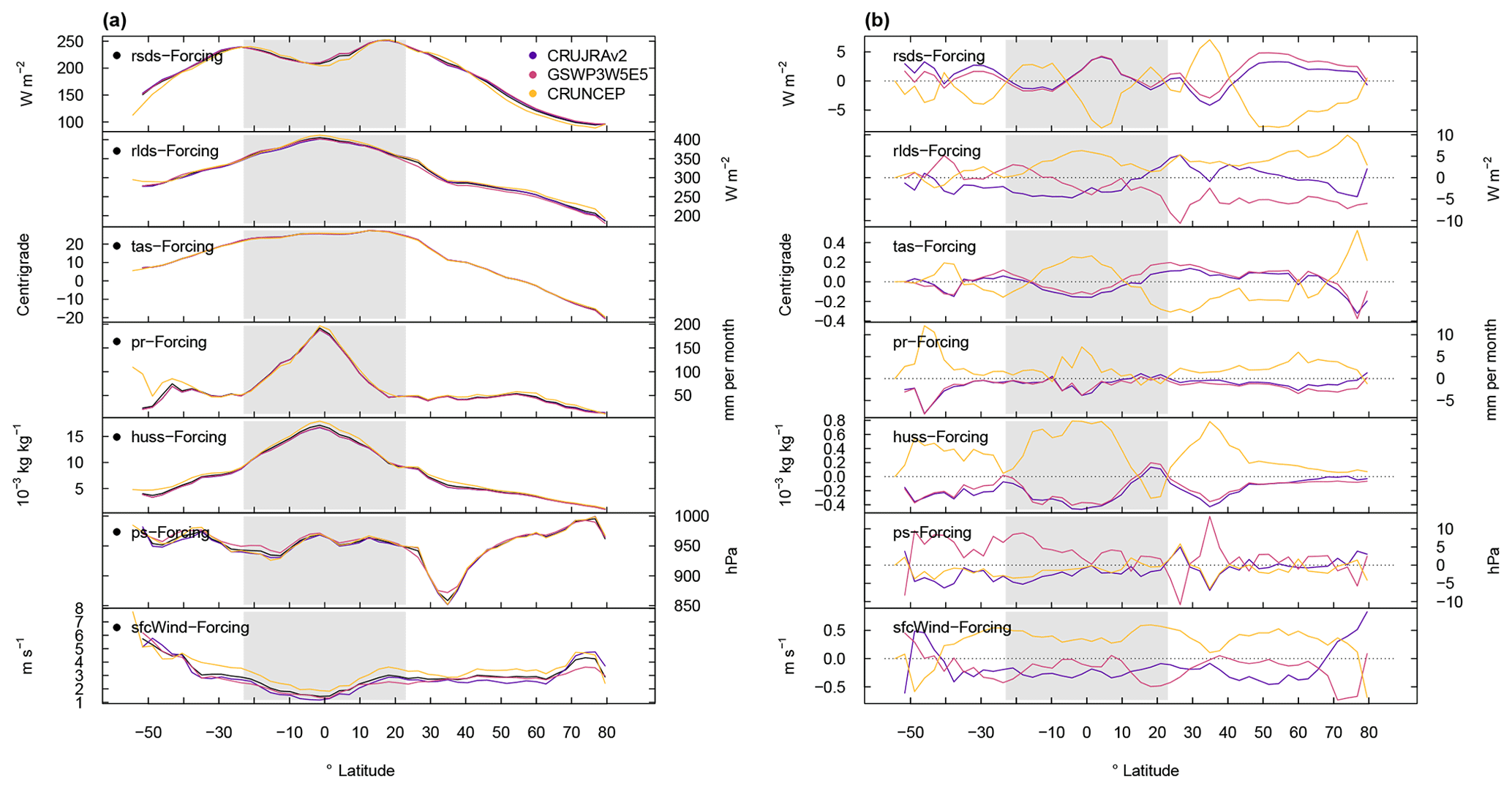
Figure A1 (a) Zonal mean values of meteorological forcing data and (b) corresponding difference between the individual forcing and the mean of the three forcings, where rsds and rlds are the surface downwelling SW and LW radiation, respectively, tas is the near-surface air temperature, pr is the precipitation, huss is the near-surface specific humidity, ps is the surface pressure, and sfcWind is the near-surface wind speed.

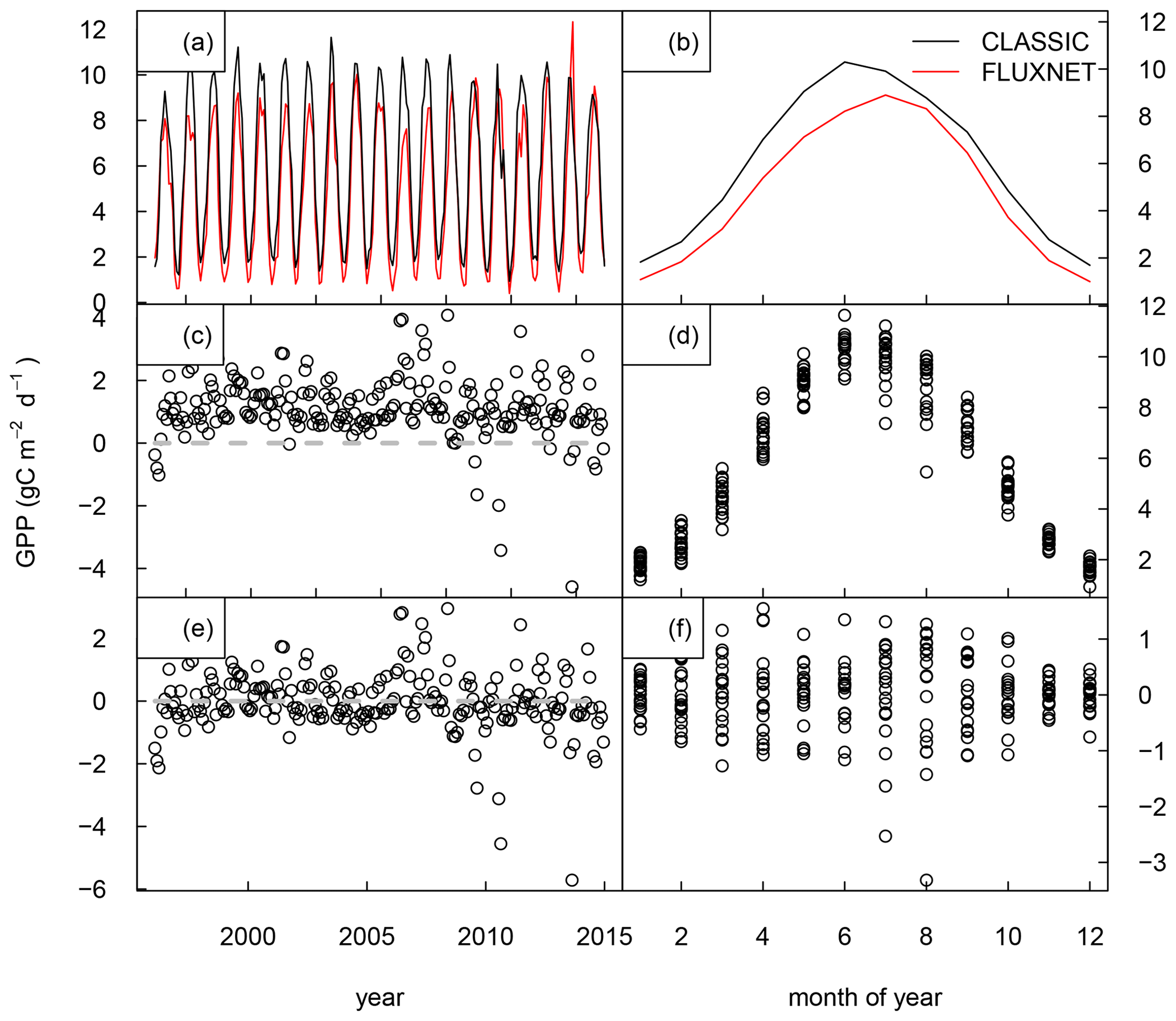
Figure A2 The left-hand column shows monthly values of (a) modeled (black) and observed (red) gross primary productivity, (c) residuals, and (e) residuals of the anomalies. The right-hand column gives the corresponding model values for the (b) climatological mean seasonal cycle, (d) monthly variability, and (f) monthly variability of anomalies. The data correspond to CLASSIC model output for the location of an eddy covariance measurement site in the Netherlands (NL-Loo).

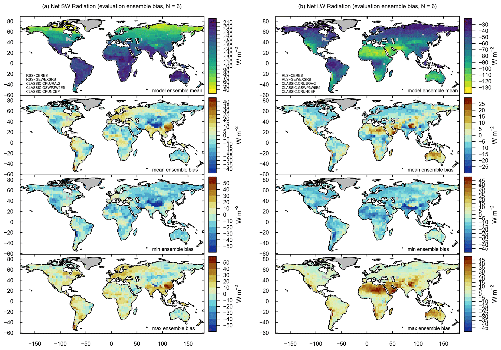
Figure A3 Same as Fig. 7 but for (a) net SW radiation and (b) net LW radiation.

Figure A4 Same as in Fig. 8 but for net SW radiation.

Figure A5 Same as in Fig. 8 but for net LW radiation.

Figure A6 Same as in Fig. 8 but for surface albedo.

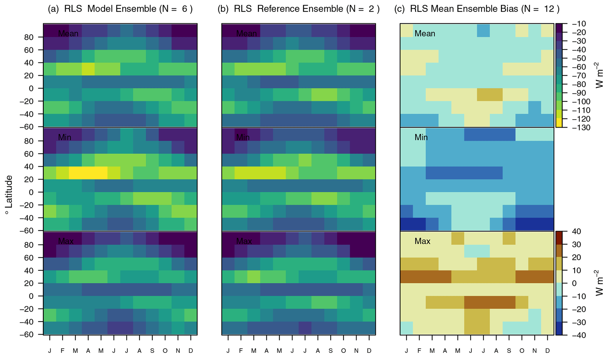
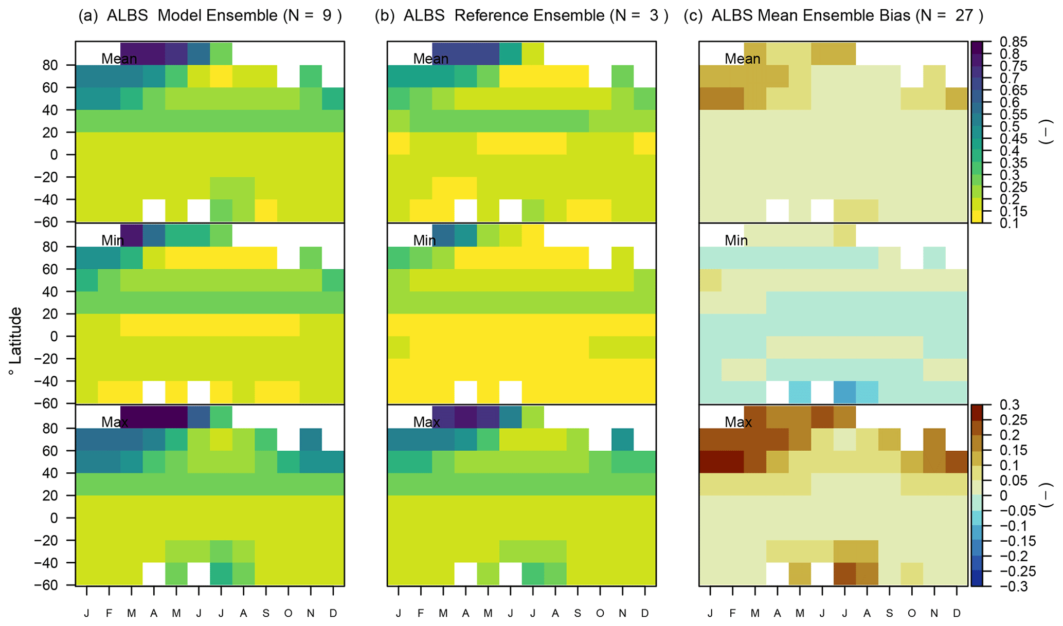
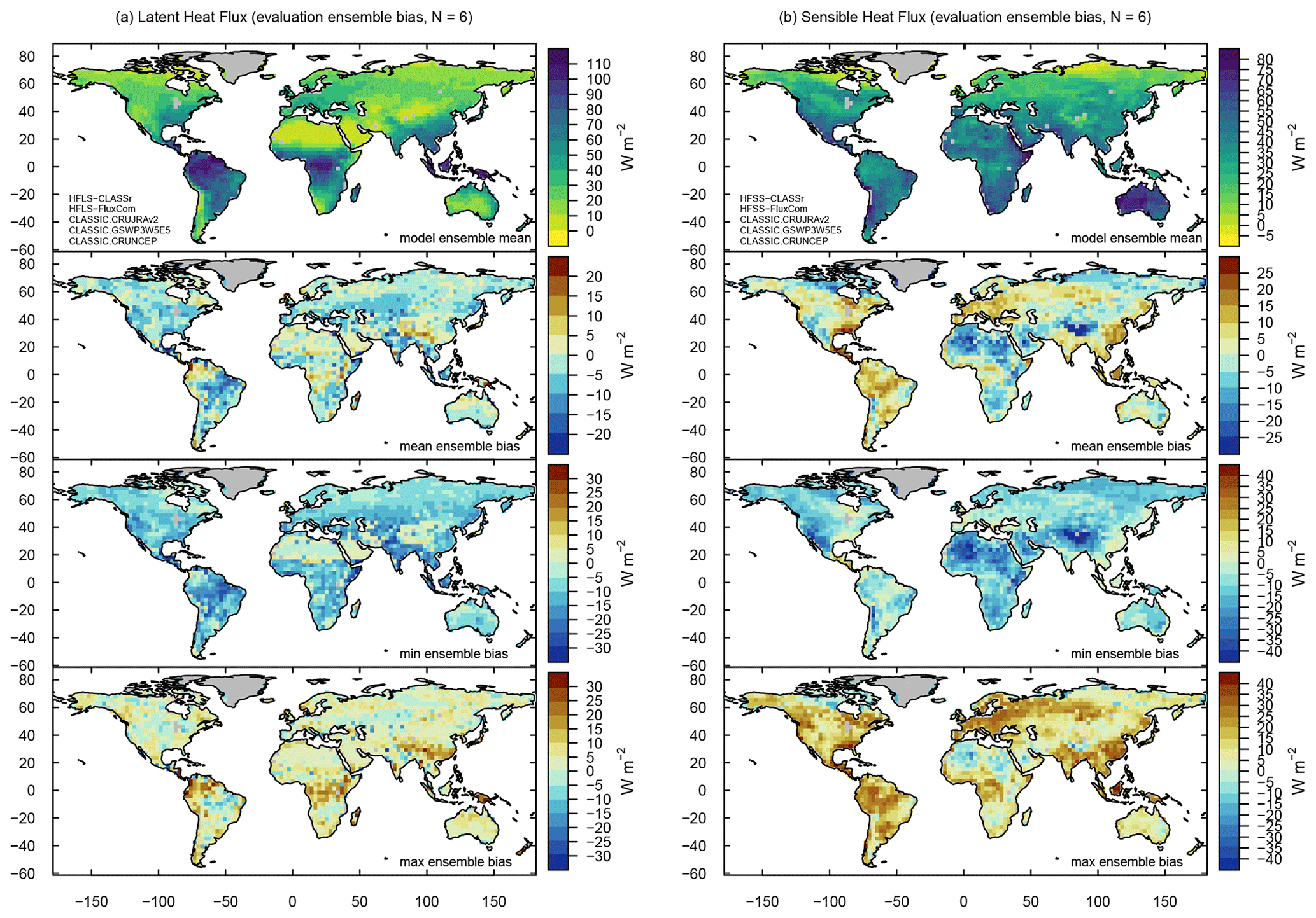
Figure A7 Same as Fig. 7 but for (a) latent heat flux and (b) sensible heat flux.

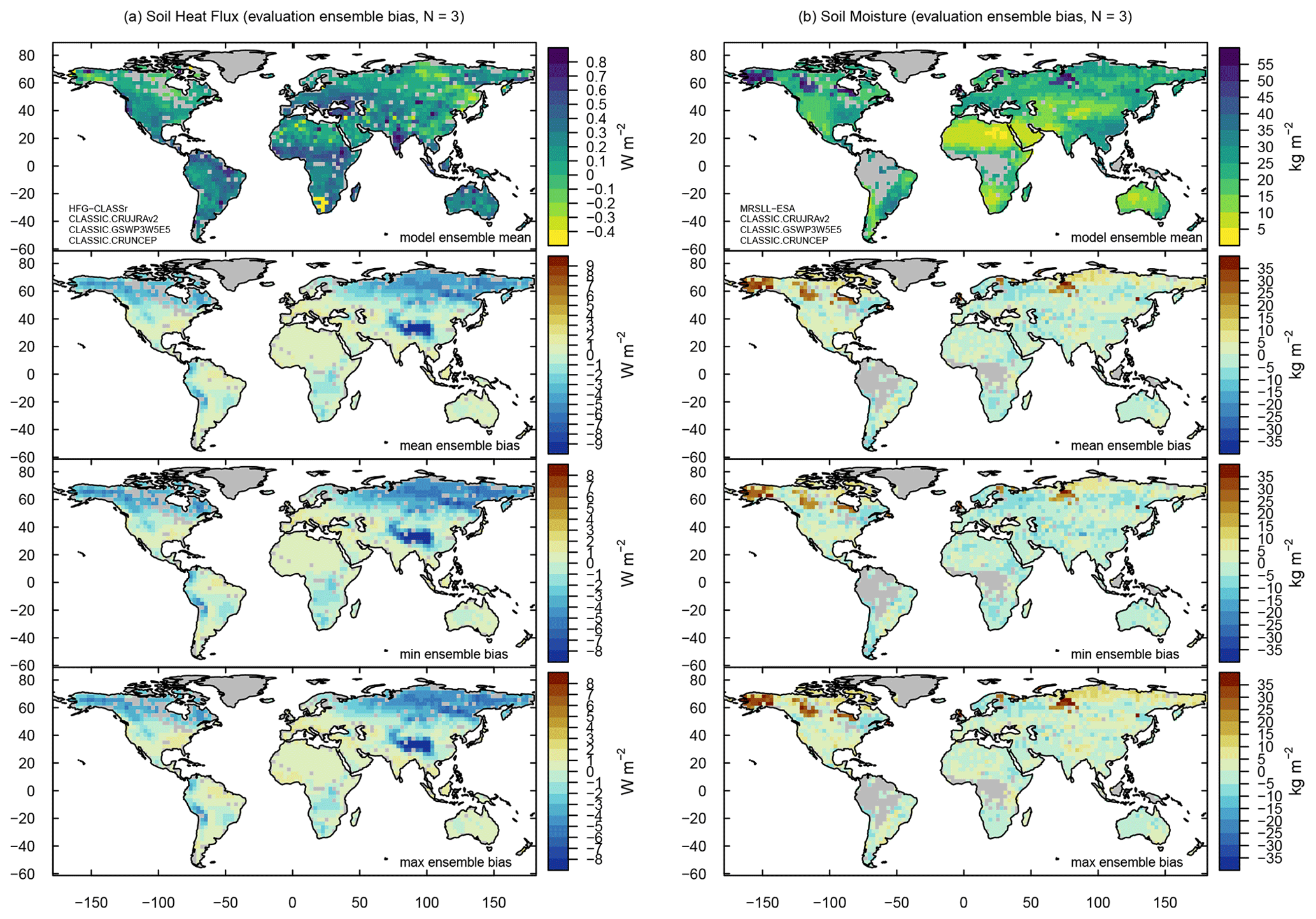
Figure A8 Same as Fig. 7 but for (a) soil heat flux and (b) soil moisture in the top 10 cm.

Figure A9 Same as in Fig. 8 but for sensible heat flux.

Figure A10 Same as in Fig. 8 but for latent heat flux.

Figure A11 Same as in Fig. 8 but for soil heat flux.

Figure A12 Same as in Fig. 8 but for soil moisture.

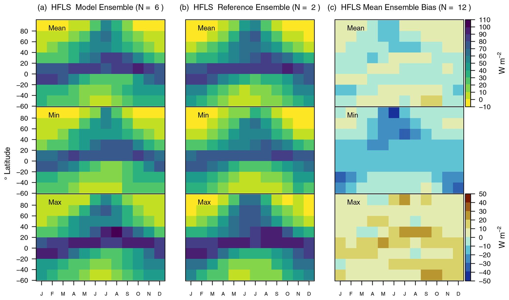
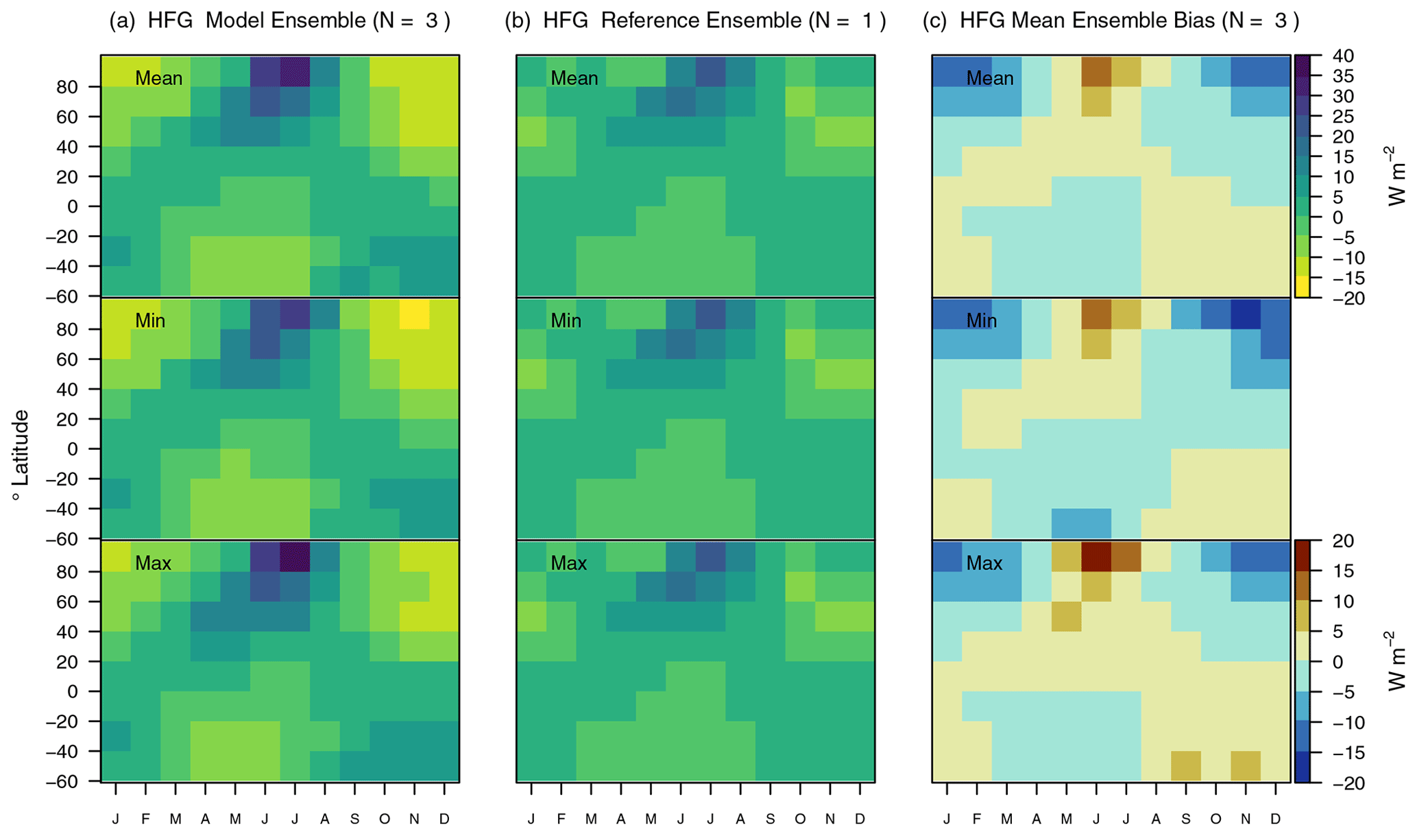
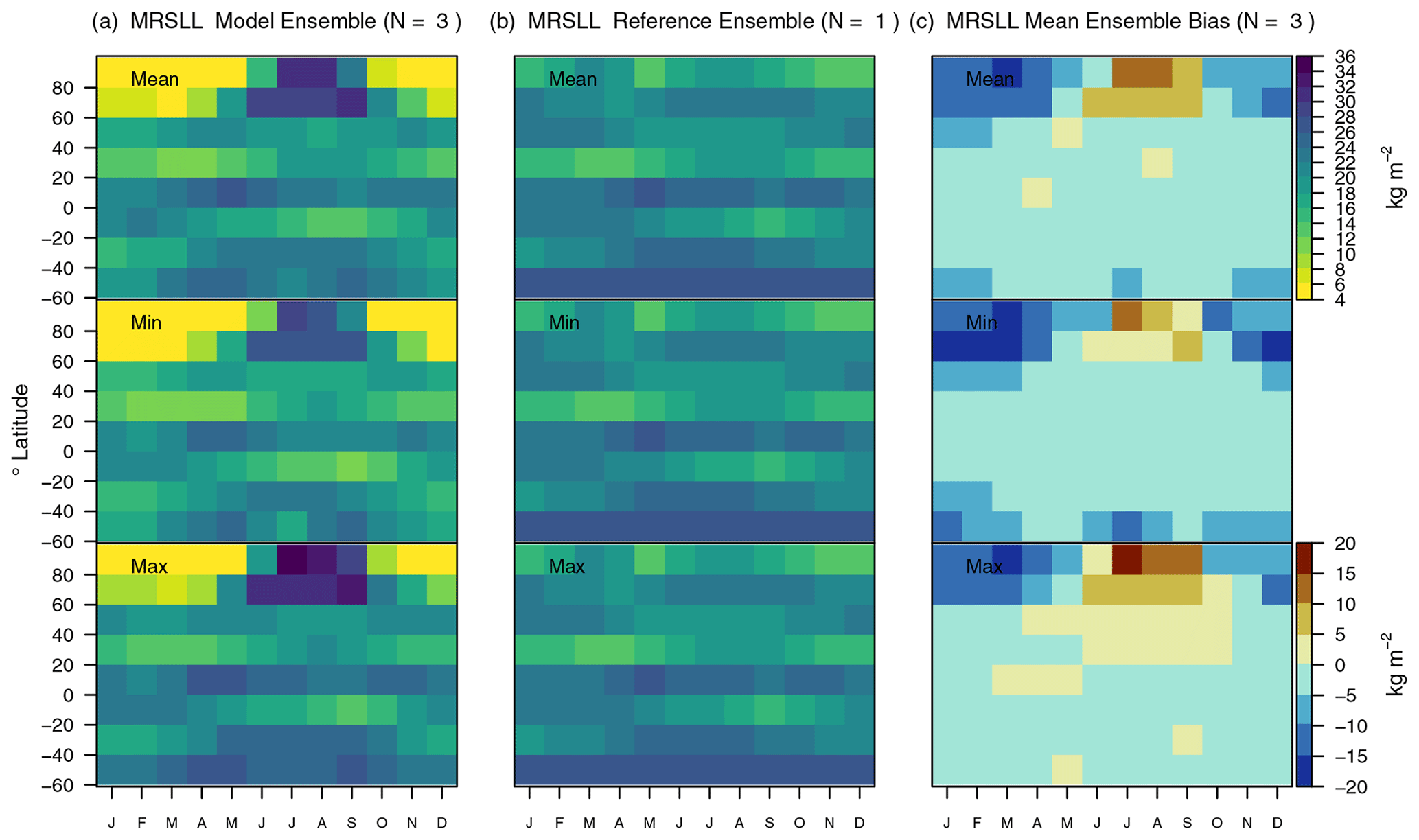
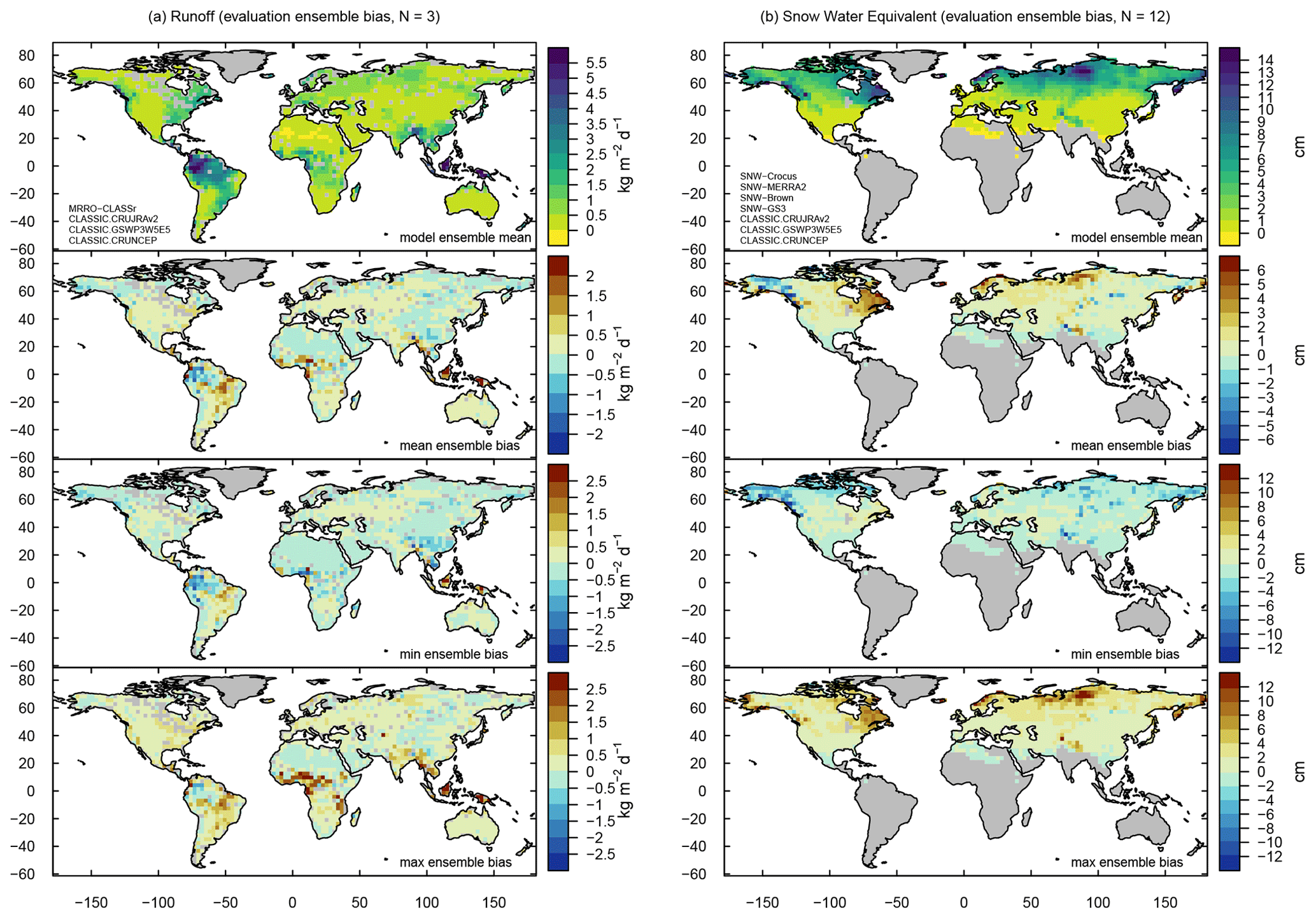
Figure A13 Same as Fig. 7 but for (a) runoff and (b) snow water equivalent.

Figure A14 Same as in Fig. 8 but for runoff.

Figure A15 Same as in Fig. 8 but for snow water equivalent.

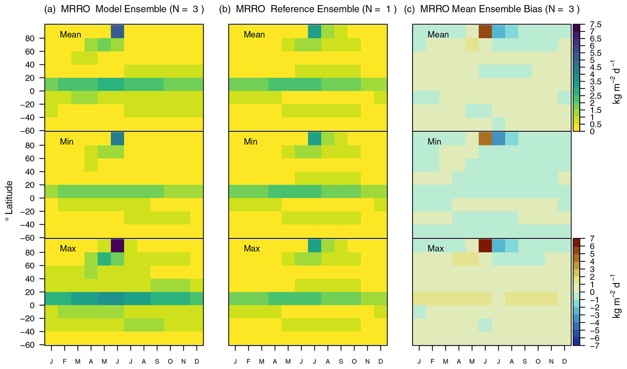
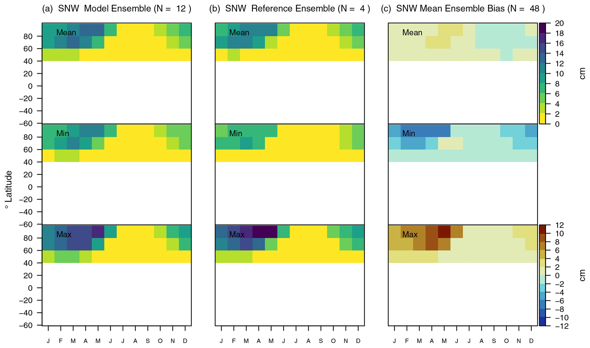
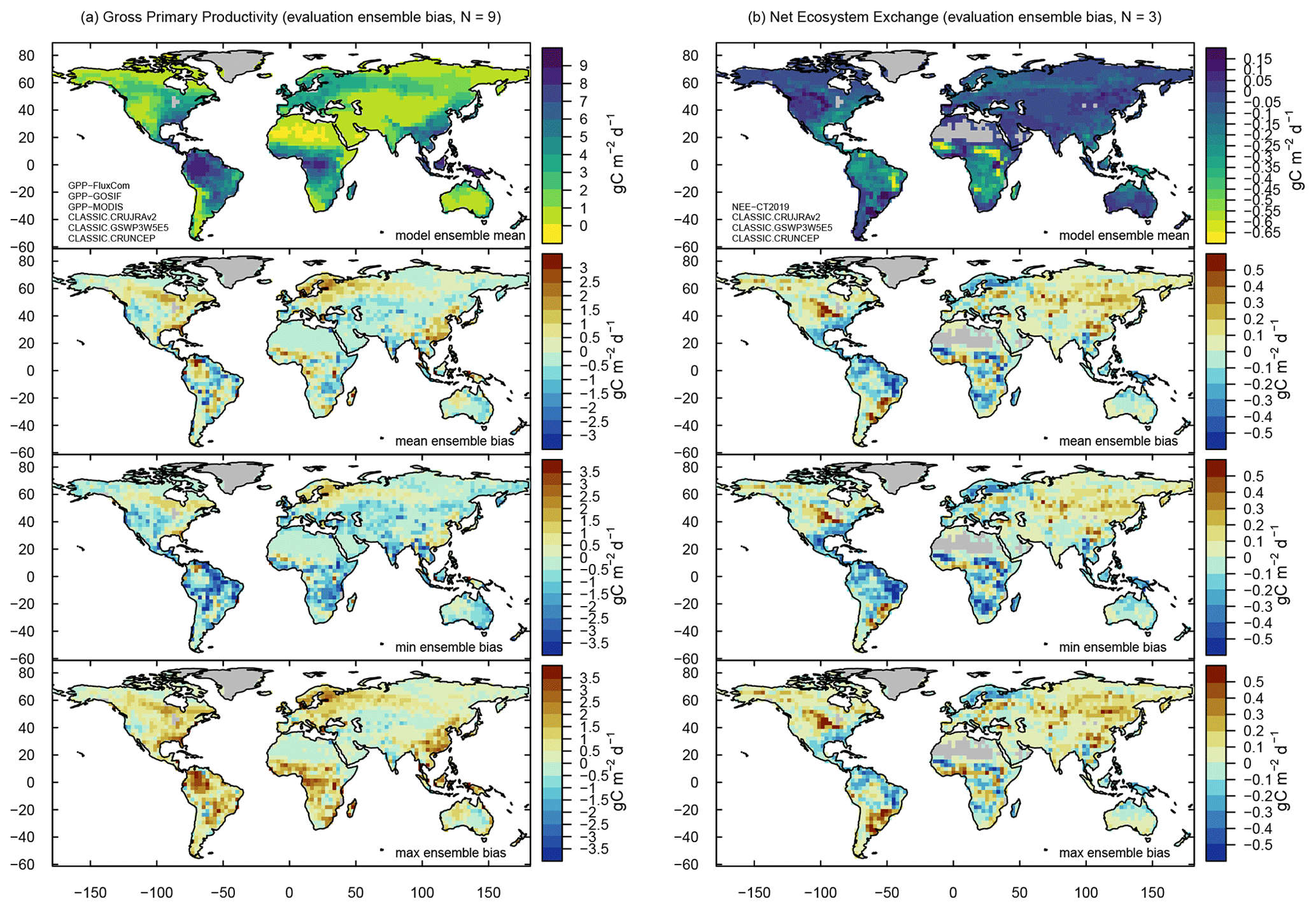
Figure A16 Same as Fig. 7 but for (a) gross primary productivity and (b) net ecosystem exchange.

Figure A17 Same as in Fig. 8 but for gross primary productivity.

Figure A18 Same as in Fig. 8 but for net ecosystem exchange.

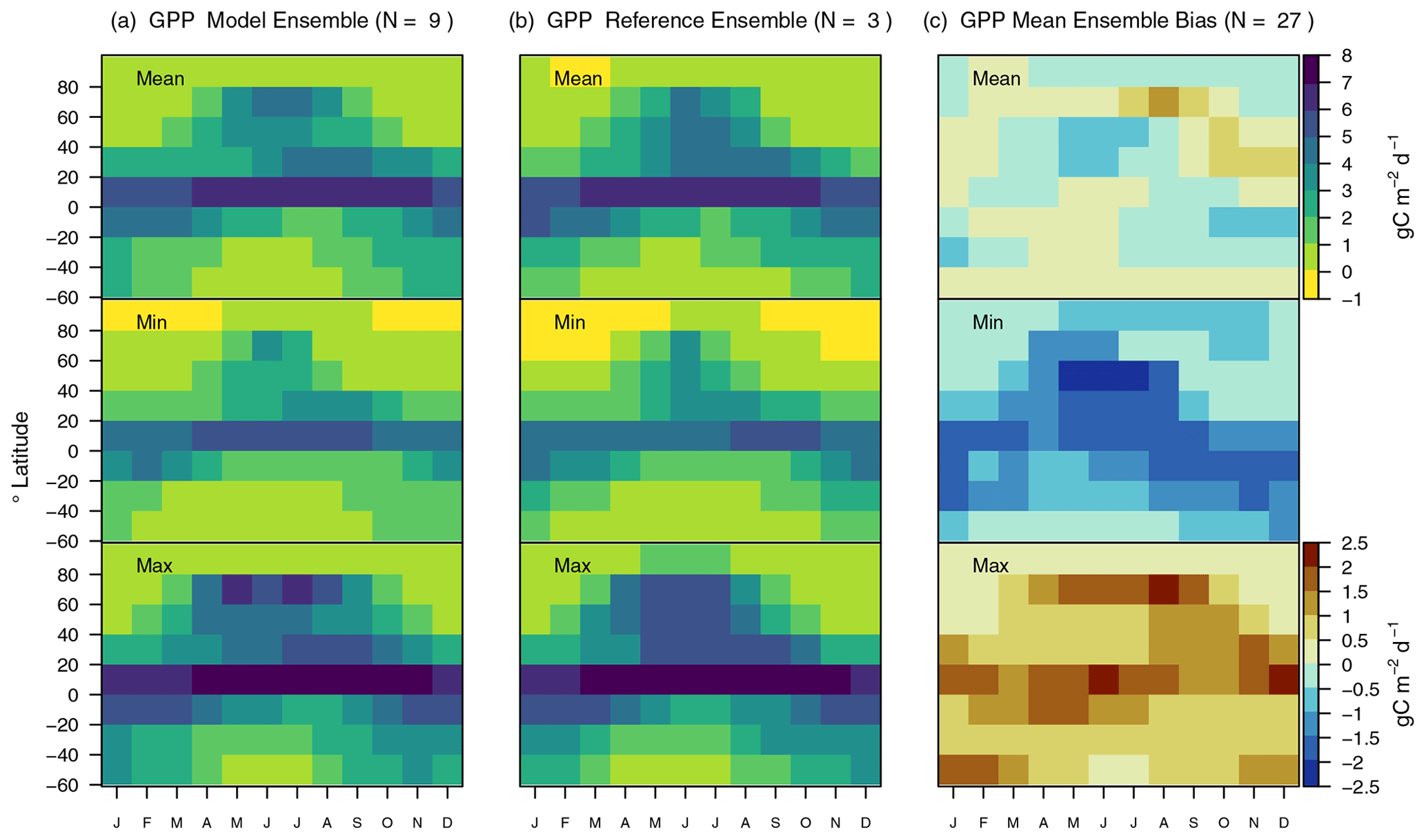
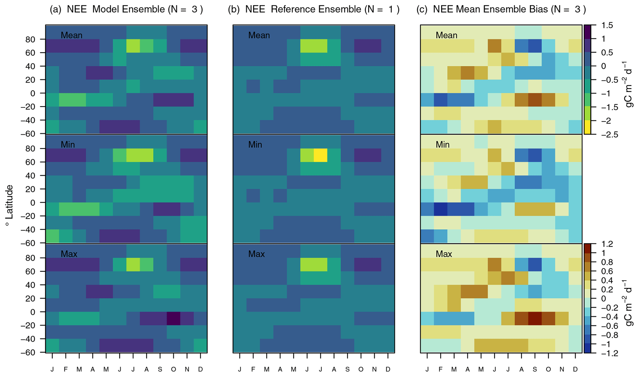
Figure A19 Same as Fig. 7 but for (a) fractional area burned and (b) emissions from wildfires.

Figure A20 Same as in Fig. 8 but for fractional area burned.

Figure A21 Same as in Fig. 8 but for emissions from wildfires.

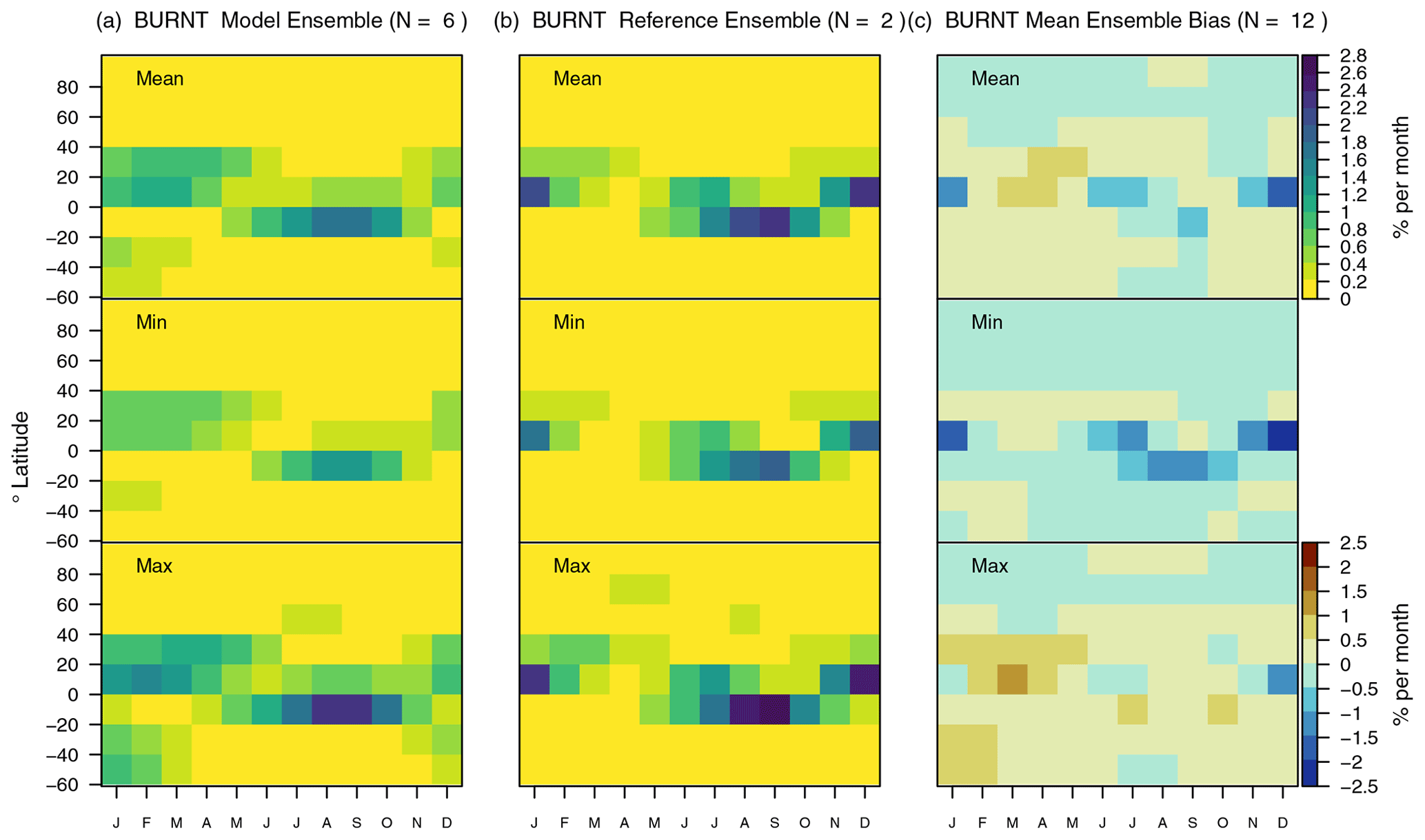
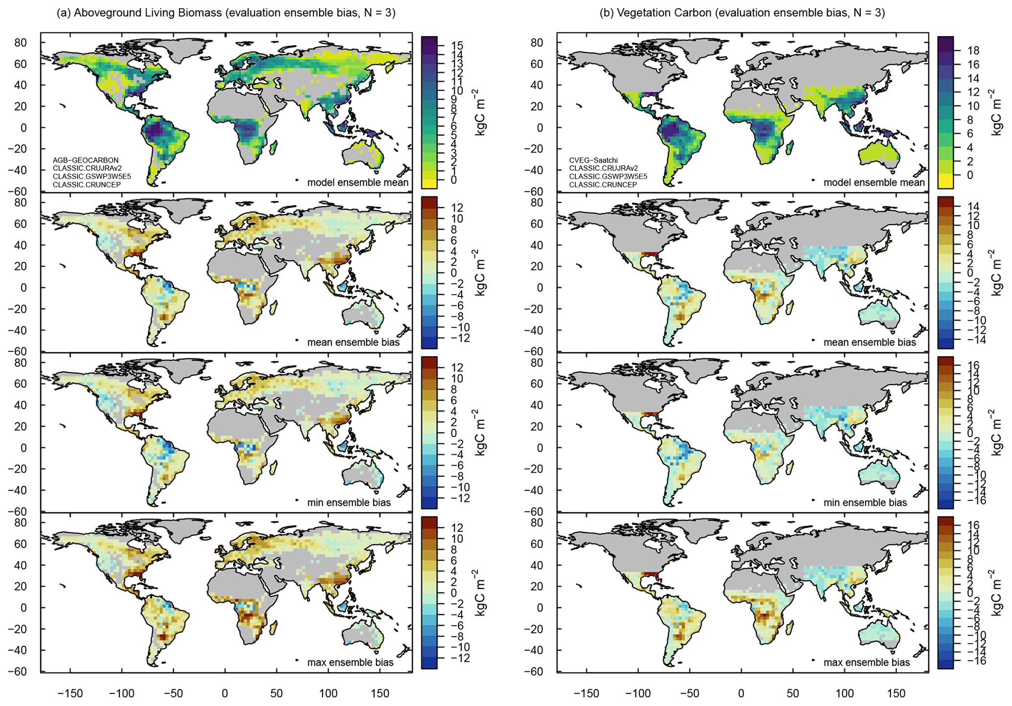
Figure A22 Same as Fig. 7 but for (a) above-ground living biomass and (b) vegetation carbon in the tropics.

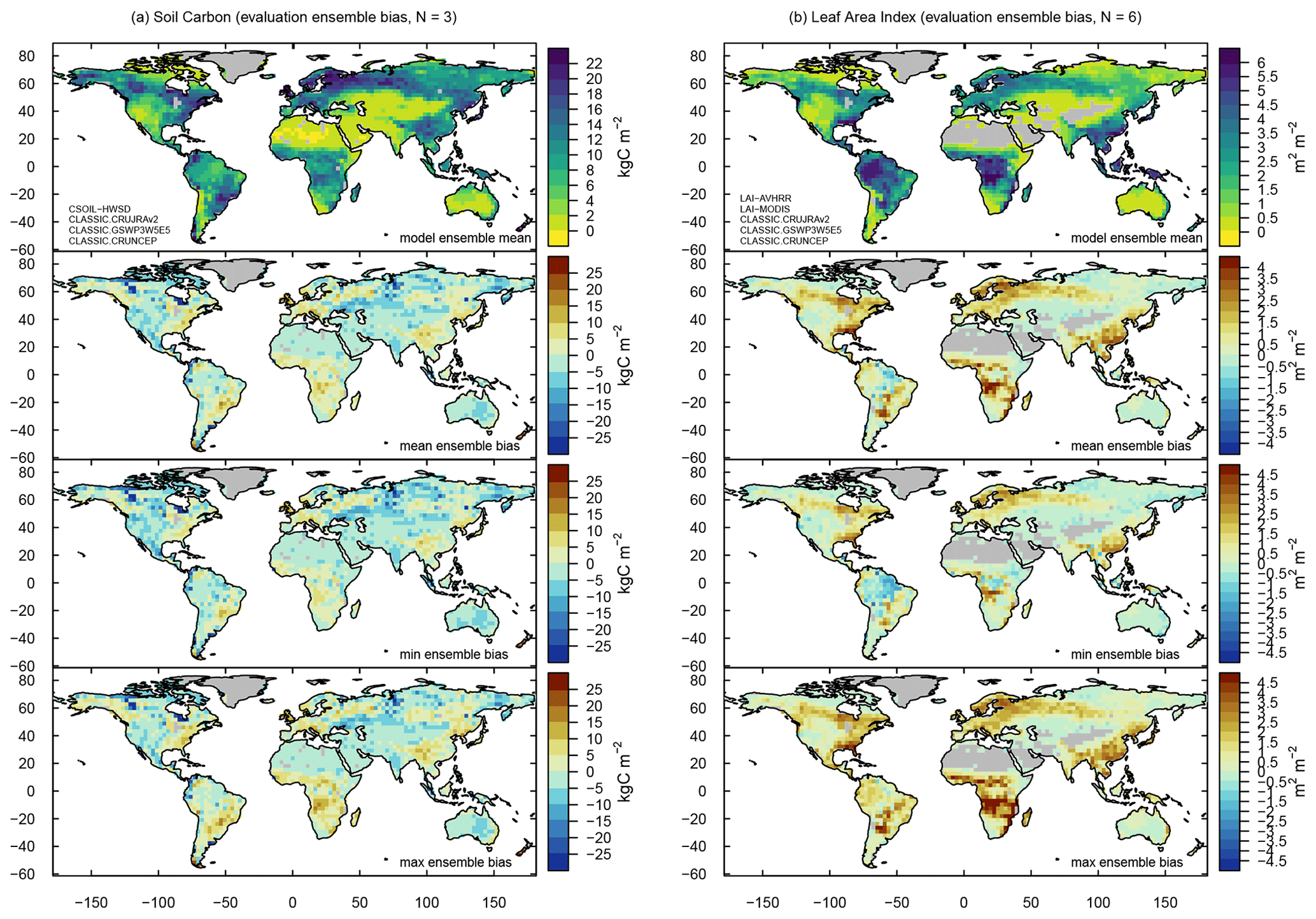
Figure A23 Same as Fig. 7 but for (a) soil organic carbon mass and (b) leaf area index.

Figure A24 Same as in Fig. 8 but for leaf area index.

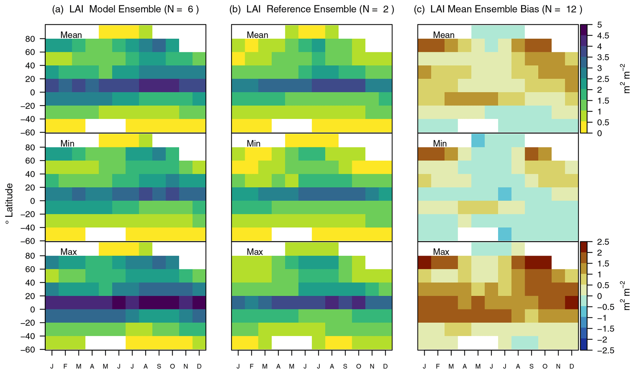
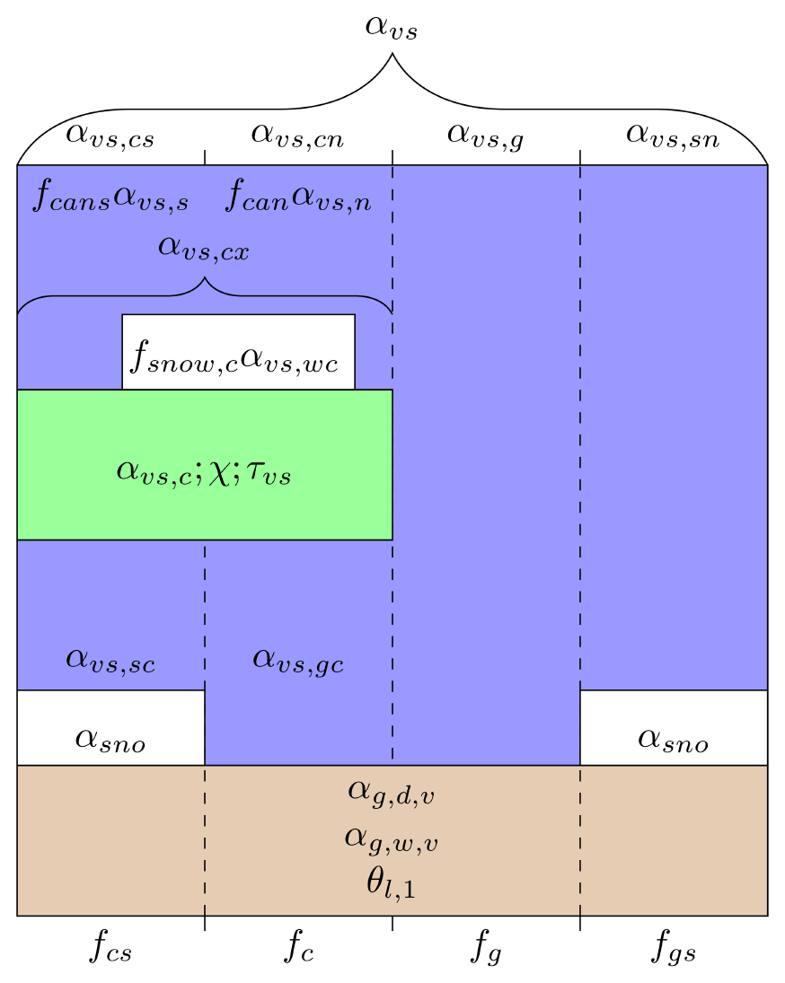
Figure A25 Contributions from the bare ground (brown), canopy (green), and snow (white) to the total visible albedo of the land surface. All variables are defined in the Appendix.

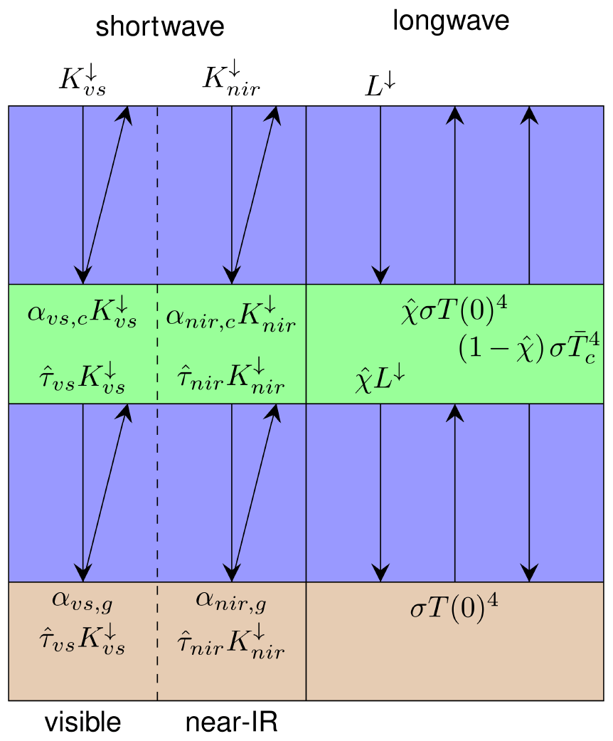
Figure A26 Longwave and shortwave radiation fluxes between the ground (brown), canopy (green), and overlying atmosphere. The meaning of each arrow is given at its tail. All variables are defined in the Appendix.