Dynamical Madden–Julian Oscillation forecasts using an ensemble subseasonal-to-seasonal forecast system of the IAP-CAS model

The Madden–Julian Oscillation (MJO) is a crucial predictability source on a subseasonal-to-seasonal (S2S) timescale. Therefore, the models participating in the World Weather Research Programme and the World Climate Research Programme (WWRP/WCRP) S2S prediction project focus on accurately predicting and analyzing the MJO. This study provides a detailed description of the configuration within the Institute of Atmospheric Physics at the Chinese Academy of Sciences (IAP-CAS) S2S forecast system. We assess the accuracy of the IAP-CAS model's MJO forecast using traditional Real-time Multivariate MJO (RMM) analysis and cluster analysis. Then, we explain the reasons behind any bias observed in the MJO forecast. Comparing the 20-year hindcast with observations, we found that the IAP-CAS ensemble mean has a skill of 24 d. However, the ensemble spread still has potential for improvement. To examine the MJO structure in detail, we use cluster analysis to classify the MJO events during boreal winter into four types: fast-propagating, slow-propagating, standing, and jumping patterns of MJO. The model exhibits biases of overestimated amplitude and faster propagation speed in the propagating MJO events. Upon further analysis, it was found that the model forecasted a wetter background state. This leads to stronger forecasted convection and coupled waves, especially in the fast MJO events. The overestimation of the strength and length of MJO-coupled waves results in a faster MJO mode and quicker dissipation in the IAP-CAS model. These findings show that the IAP-CAS skillfully forecasts signals of MJO and its propagation, and they also provide valuable guidance for improving the current MJO forecast by developing the ensemble system and moisture forecast.

1 Introduction

With the increasing occurrence of metrological disasters in recent years, there has been growing attention on subseasonal-to-seasonal (S2S) forecasts, as these forecasts bridge the gap between weather and climate forecasts and reduces disaster risks through early warnings. In November 2013, the WWRP/WCRP S2S prediction project (Phase 1) was launched, with the principal objectives of enhancing S2S forecast accuracy and advancing our comprehension of its dynamics and climate drivers. Then, work on S2S research continued in Phase 2, from 2018 to 2023. The whole project has made a significant contribution to the development of S2S prediction.

The Madden–Julian Oscillation (MJO) (Madden and Julian, 1971) is a crucial predictability source of S2S forecasts. It is a significant tropical oscillation with a period of 30–60 d, characterized by expansive cloud masses and precipitation systems that propagate eastward along the equatorial regions. Accurate S2S prediction requires a good representation of MJO. Many studies have clarified the relationship between the MJO and global weather and climate, such as monsoons (Goswami, 2012; Hsu, 2012; Lau and Chan, 1986; Wheeler et al., 2009; Liu et al., 2022), tropical cyclones (Bessafi and Wheeler, 2006; Ferreira et al., 1996; Hall et al., 2001), and the El Niño–Southern Oscillation (ENSO; Lau and Waliser, 2012; Zhang, 2005). The convective and circulation anomalies associated with MJO establish intricate connections across global weather and climate systems on the S2S timescale. Being able to accurately forecast the MJO can have a positive impact on the forecast of other related systems (Cassou, 2008; Vitart and Molteni, 2010; Wu et al., 2007). Achieving an accurate forecast of MJO has become a primary objective in the field of S2S forecasts.

With an enhanced comprehension of the underlying physical mechanisms governing the MJO and the continuous improvement of numerical models, remarkable advancements have been achieved in the MJO forecast. In Coupled Model Intercomparison Project Phase 6 (CMIP6), models that exhibited lower forecast skills (Hung et al., 2013) in Coupled Model Intercomparison Project Phase 5 (CMIP5) have demonstrated noteworthy improvements in the simulation of MJO (Chen et al., 2022). Generally, the models in CMIP6 simulate more realistic eastward propagation and precipitation over the Maritime Continent (MC) region (Ahn et al., 2020).

However, for S2S forecasts, the improvement of model physics is one aspect of advancing S2S forecasts, as various factors impact MJO forecast skills, such as initialization and ensemble generation (Kim et al., 2018). The forecast skills of the MJO in most models are typically 3–4 weeks (Vitart, 2017), while the estimate of predictability of MJO is approximately 5–7 weeks (Waliser et al., 2003; Neena et al., 2014). These facts underscore the persisting challenges in the S2S forecasts.

The realistic forecast of MJO eastward propagation is one of the challenges that have been repeatedly mentioned in recent years (Jiang, 2017; Kim, 2019; Lim et al., 2018; Wang and Lee, 2017). The MJO propagation skill is closely related to the forecast of the state in the Maritime Continent (MC) region (Gonzalez and Jiang, 2017). Many studies have pointed out the “MC barrier” (Hendon and Salby, 1994; Rui and Wang, 1990; Vitart et al., 2017) during the MJO's propagation through the MC region. The MC barrier refers to a notable deterioration of the MJO signal when it traverses the MC area, but this phenomenon is usually amplified in the climate models (H.-M. Kim et al., 2014; Neena et al., 2014; Xiang et al., 2022, 2015), showing the model's limitation in preserving MJO propagation within the MC region. The moisture mode theory (Raymond and Fuchs, 2009) has been proposed to explain this phenomenon. It suggests that the advection of seasonal mean moisture by the MJO-related circulation anomalies in the lower troposphere is crucial to MJO's propagation through the MC region (Jiang, 2017; Kim, 2019). In models that struggle to capture the realistic propagation of MJO, the mean low-troposphere moisture amplitude over the MC is underestimated, resulting in a weakened horizontal moisture gradient (Gonzalez and Jiang, 2017; Kim, 2017). This discrepancy in moisture advection hinders MJO propagation.

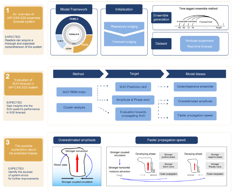
The Institute of Atmospheric Physics at the Chinese Academy of Sciences (IAP-CAS) has been actively involved in climate model development and applications since CMIP1 in the 1990s. As for the IAP-CAS model, it has already shown a significant enhancement in MJO simulation in CMIP6 compared to CMIP5 (Chen et al., 2022), but the performance of the S2S system in IAP-CAS remains uncertain and requires comprehensive evaluation. Therefore, the objectives of this article are fourfold. Firstly, we introduce the S2S forecast system of the IAP-CAS model. Secondly, we evaluate the forecast skills of the IAP-CAS in the MJO forecast. Thirdly, we analyze the evaluation results to identify the sources of forecast errors, facilitating further improvements in the MJO forecast. Lastly, we hope that the verification and analysis process can provide some valuable insights for other models.

The structure of the paper is as follows. A thorough review of the IAP-CAS model and S2S ensemble forecast system is introduced in Sect. 2. Section 3 describes the observation data and primary methodology utilized in the article. Section 4 assesses the overall MJO forecast skills in IAP-CAS. Section 5 focuses on analyzing the propagation details of the fast-propagating and slow-propagating MJO. After that, in Sect. 6, we discuss the potential causes of any bias observed in the MJO forecast. In Sect. 7, we summarize our findings and discuss the results.

Figure 1 The structure of the IAP-CAS S2S ensemble forecast system.

2 The global S2S ensemble forecast system of IAP-CAS

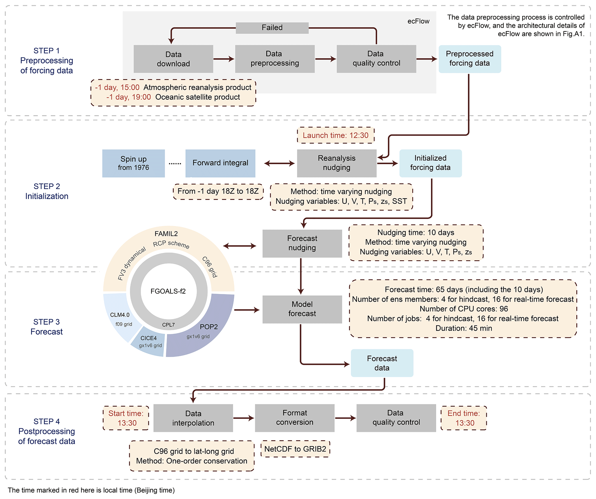
The architecture of the IAP-CAS S2S ensemble forecast system is depicted in Fig. 1. In this section, we give a thorough description of the S2S system, covering the model, initialization methods, ensemble generation approaches, and the resulting datasets.

2.1 Configuration of the IAP-CAS model

The Chinese Academy of Sciences Flexible Global Ocean–Atmosphere–Land System Finite-Volume version 2 (CAS FGOALS-f2) climate system model (Bao, 2019; Bao et al., 2020) is the core of the IAP-CAS S2S ensemble forecast system. It was developed by the State Key Laboratory of Numerical Modeling for Atmospheric Sciences and Geophysical Fluid Dynamics (LASG) at the Institute of Atmospheric Physics (IAP), Chinese Academy of Sciences (CAS). We utilize the institution name, IAP-CAS, as a proxy for the model.

Table 1 Configuration of the coupled climate system model CAS FGOALS-f2.

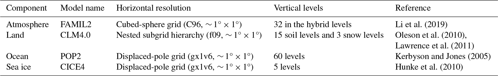
FGOALS-f2 is a fully coupled model that encompasses four components: atmospheric, land, oceanic, and sea ice models, with its configuration detailed in Table 1. The atmospheric component is version 2 of the Finite-volume Atmospheric Model (FAMIL2; Li et al., 2019), with a standard horizontal resolution of C96, which means 96 × 96 grid points in each tile of the cube sphere, roughly equivalent to 1° resolution. Vertically, it features 32 hybrid sigma-pressure levels, with the uppermost level situated at 1 hPa (the hybrid coefficients are listed in Table A1). The land surface component used in FGOALS-f2 is version 4 of the Community Land Model (CLM4.0; Oleson et al., 2010; Lawrence et al., 2011), featuring a horizontal resolution nearly at 1° resolution. The oceanic component is the Parallel Ocean Program version 2 (POP2; Kerbyson and Jones, 2005), which utilizes a displaced-pole grid with the North Pole shifted to Greenland. This grid has a resolution of gx1v6, approximately equivalent to a 1° horizontal resolution, and includes 60 vertical layers. The sea ice component is the Los Alamos Sea Ice Model version 4.0 (CICE4; Hunke et al., 2010), sharing the same horizontal resolution as the ocean model. These four components are coupled via the coupler version 7 in the Community Earth System Model (CESM; Craig et al., 2012).

Figure 2 The initialization scheme of the S2S ensemble forecast system in the IAP-CAS model. The relaxation coefficient (N) as a function of time (t) in (a) the reanalysis nudging and (b) the forecast nudging. In (a), the reanalysis nudging begins on 1 January 1976. The dots indicate the nudging process every 30 min. In (b), the solid lines of four colors represent the four ensemble members with their generation facilitated through the application of the time-lagged method.

It is worth noting that FAMIL2, the latest-generation atmospheric model from LASG, has adopted the Finite-Volume Cubed-Sphere Dynamical Core (FV3; Lin, 2004; Putman and Lin, 2007; Harris et al., 2020) as its dynamical core. FV3 solves the fully compressible Euler equations on the gnomonic cubed-sphere grid and a Lagrangian vertical coordinate. The hydrostatic solver of FV3 is used in our model. This enhancement of the atmospheric component results in improved computational efficiency and accuracy. Moreover, the key parameterization in FAMIL2 is a resolved convection precipitation (RCP) scheme, which is independently developed to calculate the microphysics processes in the convective precipitation for both deep and shallow convection (Bao and Li, 2020). Due to the rapid phase changes occurring within the convective cloud, a sub-time step of 150 s is employed for the calculation of microphysical processes within a physical time step of 30 min. FAMIL2 has also implemented the University of Washington Moist Turbulence (UWMT) parameterization scheme (Park and Bretherton, 2009) as its boundary layer scheme. The microphysical parameterization used in FAMIL2 is the revised Lin scheme, which is a single-moment scheme (Zhou et al., 2019).

2.2 Initialization scheme of the S2S forecast system

The S2S forecast system of the IAP-CAS model adopts a Newtonian nudging method with time-varying treatment (Jeuken et al., 1996) to complete the initialization of the atmosphere and ocean. The reanalysis nudging and the forecast nudging are the two components that make up the initialization process, which is seen in Fig. 2. Table A2 provides a summary of the detailed technical specifics for these two nudging processes.

The reanalysis nudging initializes the atmospheric variables, including temperature, surface pressure, sea level pressure, and surface wind, from the NCEP Final (FNL) Operational Global Analysis datasets (National Centers for Environmental Prediction/National Weather Service/NOAA/U.S. Department of Commerce, 2000). The oceanic variable of potential temperature from the National Oceanic and Atmospheric Administration (NOAA) Optimum Interpolation Sea Surface Temperature (OISST) reanalysis data (Reynolds et al., 2007) is also included. These reanalysis data serve as observations in Eq. (1) to diminish errors in the initial condition:

$$\begin{array}{}\text{(1)}& x\left(t\right)=x_{\text{model}}\left(t\right)+N_{\text{rea}}\left(t\right)\left[x_{\text{obs}}\right(t)-x_{\text{model}}(t\left)\right],\end{array}$$

where t is the time; x(t) is the value after the nudging process; x_model(t) represents the model forcing; x_obs(t) represents the “truth” value; and N_rea(t) is a relaxation coefficient that varies over time, which constantly adjusts the model results during the integration process, making it approximate to the observed values while being constrained by the dynamical constraints of the physical model. The calculation process for N_rea(t) is as follows:

$$\begin{array}{}\text{(2)}& N_{\text{rea}}\left(t\right)={\displaystyle \frac{\mathrm{\Delta }t}{\frac{T}{\mathrm{1}+\cos (\mathrm{2}\mathit{\pi }\cdot \frac{t\mathit{\%}T}{T})}+\mathrm{\Delta }t}}.\end{array}$$

Here, Δt is the time step in FAMIL2, which is 0.5 h for C96 resolution (approximately 1° resolution). T represents the time window with a value of 6 h. As depicted in Fig. 2a, the relaxation coefficient varies as a cosine function. It is large at the beginning and end of the temporal window, thereby facilitating accelerated convergence of the model results toward observations, while in the middle of the time window, N_rea becomes smaller and even drops to 0, which indicates the reliability of the reanalysis data decreases. The reason is that the reanalysis data within the time window are obtained through interpolation between its start and end values.

In the forecast nudging, the initialization process adheres to a similar nudging algorithm at 6 h intervals, as shown in Eq. (3).

$$\begin{array}{}\text{(3)}& x\left(t\right)=x_{\text{model}}\left(t\right)+N_{\text{fcst}}\left(t\right)\left[x_{\text{fcst}}\right(t)-x_{\text{model}}(t\left)\right]\end{array}$$

Nevertheless, the atmospheric variables assimilated into the S2S system are sourced from the Global Forecast System (GFS) weather forecast, denoted as x_fcst(t). The relaxation coefficient N_fcst(t) is as follows:

$$\begin{array}{}\text{(4)}& N_{\text{fcst}}\left(t\right)={\displaystyle \frac{\mathrm{\Delta }t}{\frac{T}{\mathrm{1}+\cos (\mathrm{2}\mathit{\pi }\cdot \frac{t\mathit{\%}T}{T})}+\mathrm{\Delta }t}}\cdot \cos \left({\displaystyle \frac{\mathit{\pi }}{\mathrm{2}}}\cdot {\displaystyle \frac{(t-t\mathit{\%}T)}{\mathrm{4}mT}}\right).\end{array}$$

Compared to N_rea, N_fcst is multiplied by a decay factor, which also varies in accordance with the cosine function. In this context, the number of days for forecast nudging is denoted by m, and the system is configured with a 10 d forecast nudging period. Figure 2b illustrates the variation in N_fcst, which decreases as the reliability of weather forecast data diminishes over time, ultimately reaching 0 by the 10th day.

In forecast nudging, we used 10 d of GFS weather forecast data for nudging. One purpose of this approach is to avoid coupling shock at initialization. Additionally, we aim to enhance the quality of initial forecasts in S2S by nudging GFS weather forecast data to ultimately improve S2S prediction accuracy, as the skill of weather forecasts is higher than that of S2S forecasts during the initial period.

Summarily, the S2S forecast system commences its daily forecast from the initial condition derived via reanalysis nudging. It then fine-tunes the forecasts with weather prediction data through the forecast nudging process. This initialization system effectively reduces system errors in the model and augments forecast accuracy.

2.3 Time-lagged method for ensemble generation

The value of ensemble forecasts in medium- to long-term forecasts has been emphasized repeatedly (Liu, 2003; Vitart and Molteni, 2009). In addition to improving the physical scheme of the model, devising an effective approach for ensemble generation might have a considerable impact on the MJO forecast. The IAP-CAS S2S ensemble forecast system utilizes the time-lagged method (Hoffman and Kalnay, 1983) to generate ensemble members.

A schematic diagram of the time-lagged method is depicted in Fig. 2b. During the initial day of the forecast nudging, the S2S system issues forecasts from 00Z, 06Z, 12Z, and 18Z, resulting in the generation of four ensemble members. The core idea behind this approach is to introduce perturbations by leveraging lagged initialization times.

2.4 Hindcast experiment and real-time forecast

The S2S ensemble forecast system provides daily forecasts, forecasting weather and climate conditions for the upcoming 65 d. Out of the 65 d, 5 d are reserved for extending the ensemble members by using the time-lagged method, ensuring a complete forecast for at least 60 d. Since 1 June 2019, the IAP-CAS S2S system has been operating 16 ensemble members daily for real-time forecasts. So far, approximately 8.2 TB of real-time data has been uploaded to the S2S website. For hindcast experiments from 1999 to 2018, the system has run four ensemble members daily, generating a dataset of approximately 11 TB. Our subsequent research is based on the 20-year hindcast experiment.

In 2021, the IAP-CAS model participated in phase II of the S2S Project (Vitart et al., 2017), successfully providing the 20-year hindcast and real-time forecast data generated by the S2S ensemble forecast system. Detailed information regarding the data is listed in Table A3, and Table A4 shows the list of output variables. The output data are interpolated to a standardized horizontal resolution of 1.5° × 1.5°, following the S2S's requirements, and are stored in version 2 of the General Regularly-distributed Information in Binary (GRIB2) format. The output data of the S2S system are publicly available on three S2S data portals (ECMWF, CMA, and IRI).

3 Datasets and methods

3.1 Datasets

The observational datasets used for the MJO verification include the NOAA daily outgoing longwave radiation (OLR; Liebmann and Smith, 1996), daily wind from the National Centers for Environmental Prediction (NCEP) Department of Energy (DOE) Reanalysis 2 dataset (Kanamitsu et al., 2002), daily specific humidity from ECMWF Reanalysis version 5 (ERA5; Hersbach et al., 2023), and the precipitation product from the Global Precipitation Climatology Project (GPCP; Adler et al., 2003). To facilitate computation and meaningful comparisons, both observation and hindcast datasets have been uniformly interpolated to a horizontal resolution of 2.5° × 2.5°. Seven pressure levels (1000, 925, 850, 700, 500, 300, and 200 hPa) of wind and specific humidity are extracted for analysis.

3.2 MJO RMM index

To conduct a quantitative assessment of MJO, we have employed the widely used Real-time Multivariate MJO (RMM) index (Wheeler and Hendon, 2004) to extract the MJO signal. This index consists of two components, RMM1 and RMM2, which are the first and second principal components of the combined empirical orthogonal functions (EOFs) of multiple variables, including OLR, 200 hPa zonal wind (U200), and 850 hPa zonal wind (U850). It serves as a tool for tracking the location and amplitude characteristics of MJO.

The calculation of the RMM index refers to the method described in Gottschalck et al. (2010). Detailed calculation steps are as follows.

1. Remove zero to three wave components from the climatology and low-frequency variability of the U200, U850 and OLR variables from both the observation and hindcast data. It is noteworthy that removing low-frequency variability is to subtract the mean of the past 120 d from the anomalies. For model forecast, this is the mean model anomalies of the previous forecast days plus the mean observed anomalies of the remaining days.

2. Average the anomalies between 15° S and 15° N and normalize the three variables, using the pre-computed coefficients as in Gottschalck et al. (2010).

3. Project the anomalies onto the observed combined EOF eigenvectors from Wheeler and Hendon (2004) to get RMM1 and RMM2.

The bivariate anomaly correlation coefficient (ACC) and bivariate root mean square error (RMSE) are calculated using the observed and hindcast RMM indices to represent the forecast skills of the IAP-CAS model as

$$\begin{array}{}\text{(5)}& {\displaystyle }\mathrm{ACC}\left(\mathit{\tau }\right)={\displaystyle \frac{{\sum }_{t=\mathrm{1}}^N\left[a_{\mathrm{1}}\right(t\left)b_{\mathrm{1}}\right(t,\mathit{\tau })+a_{\mathrm{2}}(t\left)b_{\mathrm{2}}\right(t,\mathit{\tau }\left)\right]}{\begin{array}{c}\sqrt{{\sum }_{t=\mathrm{1}}^N\left[a_{\mathrm{1}}^{\mathrm{2}}\left(t\right)+a_{\mathrm{2}}^{\mathrm{2}}\left(t\right)\right]}\\ \sqrt{{\sum }_{t=\mathrm{1}}^N\left[b_{\mathrm{1}}^{\mathrm{2}}(t,\mathit{\tau })+b_{\mathrm{2}}^{\mathrm{2}}(t,\mathit{\tau })\right]}\end{array}}},\text{ and }\text{(6)}& {\displaystyle }\mathrm{RMSE}\left(\mathit{\tau }\right)=\sqrt{{\displaystyle \frac{\mathrm{1}}{N}}{\sum }_{t=\mathrm{1}}^N\left[\begin{array}{c}\left(a_{\mathrm{1}}\right(t)-b_{\mathrm{1}}(t,\mathit{\tau }){)}^{\mathrm{2}}\\ +\left(a_{\mathrm{2}}\right(t)-b_{\mathrm{2}}(t,\mathit{\tau }){)}^{\mathrm{2}}\end{array}\right]}.\end{array}$$

Here, a₁(t) and a₂(t) are the observation RMM1 and RMM2 at time t, b₁(t) and b₂(t) are the forecasting RMM1 and RMM2 at time t for lead τ days, and N is the total number of times. It is commonly accepted that days with ACC above 0.5 are considered to have valid forecasts. Therefore, the forecast skill of a model is quantitatively defined as the maximum lead time exceeding 0.5, which approximately corresponds to the day when RMSE reaches $\sqrt{\mathrm{2}}$.

The RMM index can also be adapted to quantitatively evaluate the forecasted intensity and velocity through the calculation of the error of amplitude (ERR_amp(τ)) and phase (ERR_phase(τ)) as a function of lead time τ:

$$\begin{array}{}\text{(7)}& {\displaystyle }{\mathrm{ERR}}_{\mathrm{amp}}\left(\mathit{\tau }\right)={\displaystyle \frac{\mathrm{1}}{N}}\sum \left[{\mathrm{AMP}}_{\mathrm{b}}\right(t,\mathit{\tau })-{\mathrm{AMP}}_{\mathrm{a}}(t\left)\right],\text{ and }\text{(8)}& {\displaystyle }{\mathrm{ERR}}_{\mathrm{phase}}\left(\mathit{\tau }\right)={\displaystyle \frac{\mathrm{1}}{N}}\sum {\tan }^{-\mathrm{1}}\left[{\displaystyle \frac{a_{\mathrm{1}}\left(t\right)b_{\mathrm{2}}(t,\mathit{\tau })-a_{\mathrm{2}}\left(t\right)b_{\mathrm{1}}(t,\mathit{\tau })}{a_{\mathrm{1}}\left(t\right)b_{\mathrm{1}}(t,\mathit{\tau })+a_{\mathrm{2}}\left(t\right)b_{\mathrm{2}}(t,\mathit{\tau })}}\right].\end{array}$$

Negative (positive) ERR_amp(τ) indicates weaker (stronger) amplitude in forecasts. Similarly, negative (positive) ERR_phase(τ) indicates slower (faster) propagation in forecasts. Here, the MJO amplitude for observation (AMP_a(t)) and forecast (AMP_b(t)) is defined as

$$\begin{array}{}\text{(9)}& {\displaystyle }{\mathrm{AMP}}_{\mathrm{a}}\left(t\right)=\sqrt{a_{\mathrm{1}}(t{)}^{\mathrm{2}}+a_{\mathrm{2}}(t{)}^{\mathrm{2}}},\text{ and }\text{(10)}& {\displaystyle }{\mathrm{AMP}}_{\mathrm{b}}(t,\mathit{\tau })=\sqrt{b_{\mathrm{1}}(t,\mathit{\tau }{)}^{\mathrm{2}}+b_{\mathrm{2}}(t,\mathit{\tau }{)}^{\mathrm{2}}}.\end{array}$$

3.3 Cluster analysis of MJO events

Another crucial method used in this research is cluster analysis. In Sect. 5, we select the representative MJO events and classify them following Wang et al. (2019). This facilitates a more focused and targeted investigation into the forecast bias of MJO in the IAP-CAS model.

An MJO event was chosen if the regional average of OLR, spanning 10° S to 10° N and 75 to 95° E, remained below 1 standard deviation for a consecutive period of 5 d during the boreal winter (November–April). Subsequently, the K-means cluster analysis is employed to categorize the chosen MJO events based on the propagation patterns from day −10 to 20 (day 0 is the day with the peak MJO in the Indian Ocean). We then use silhouette clustering evaluation criteria (Rousseeuw, 1987) to identify and eliminate poorly classified MJO events.

Finally, a total of 50 MJO events were selected for the winters of 1999 to 2018, and four types of MJO events were identified, namely the fast-propagating (10 cases), slow-propagating (16 cases), standing (12 cases), and jumping (12 cases) patterns of MJO (Fig. 5).

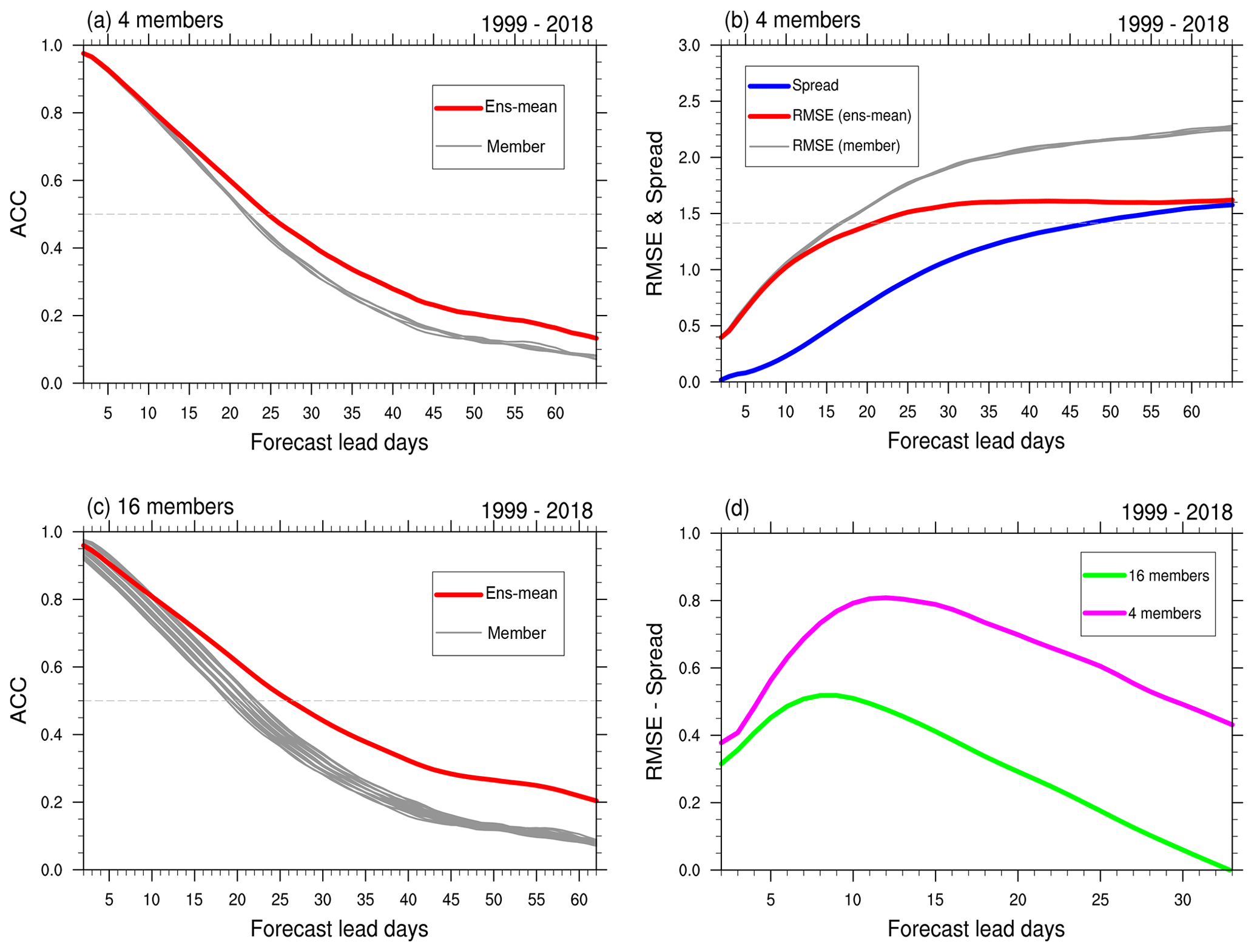
Figure 3 MJO forecast skill of IAP-CAS for the annual MJO events over 20 years (1999–2018) of reforecast data. (a) The bivariate anomalous correlation coefficient (ACC) and (b) the root mean squared error (RMSE) varied with forecast lead days for individual members (solid gray line) and ensemble mean (solid red line). The solid blue line denotes the ensemble spread. (c) The ACC of individual members and ensemble mean, as generated by the time lag method, resulting in 16 ensemble members. The dashed line in (a) and (c) has a value of 0.5, and it represents 1.414 in (b). (d) The difference between the RMSE and spread of 4-member ensemble mean (solid purple line) and 16-member ensemble mean (solid green line).

The fast-propagating MJO and slow-propagating MJO belong to the propagating type of MJO, characterized by their consecutive eastward propagation across the Indian Ocean to the Pacific Ocean region. On the other hand, the standing MJO and jumping MJO represent relatively non-propagating types, where the convection remains relatively fixed or exhibits discontinuous movement. Wang et al. (2019) believe that propagating MJO events are often associated with strong and tightly coupled Kelvin waves, especially for fast-propagating MJO. This is the biggest difference between propagating MJO and non-propagating MJO.

4 Evaluation of MJO forecast skill from the IAP-CAS model

The evaluation in this section is conducted for the annual MJO events. Figure 3 demonstrates the overall MJO forecast skill in the IAP-CAS model and the improvement brought by the time-lagged ensemble method. Figure 3a shows the forecast skill of the ensemble mean is 24 d with the criterion of ACC exceeding 0.5, while the skill of individual members is about 21–22 d. Meanwhile, the ensemble mean RMSE reaches $\sqrt{\mathrm{2}}$ at 21 d, and the individual members exhibit a larger RMSE, reaching $\sqrt{\mathrm{2}}$ at 16 d (Fig. 3b). The solid blue line in Fig. 3b represents the ensemble spread (Leutbecher and Palmer, 2008) of IAP-CAS. When this ensemble spread approaches the RMSE of the ensemble mean (solid red line), it indicates that the ensemble members are sufficiently dispersive. Figure 3b illustrates that the ensemble exhibits an underdispersive characteristic in the early stage of the forecast. We have also observed similar issues of underdispersiveness in many other models (Rashid et al., 2011; Neena et al., 2014; H.-M. Kim et al., 2014; Xiang et al., 2015), and addressing this aspect may be a focal point for future model enhancements.

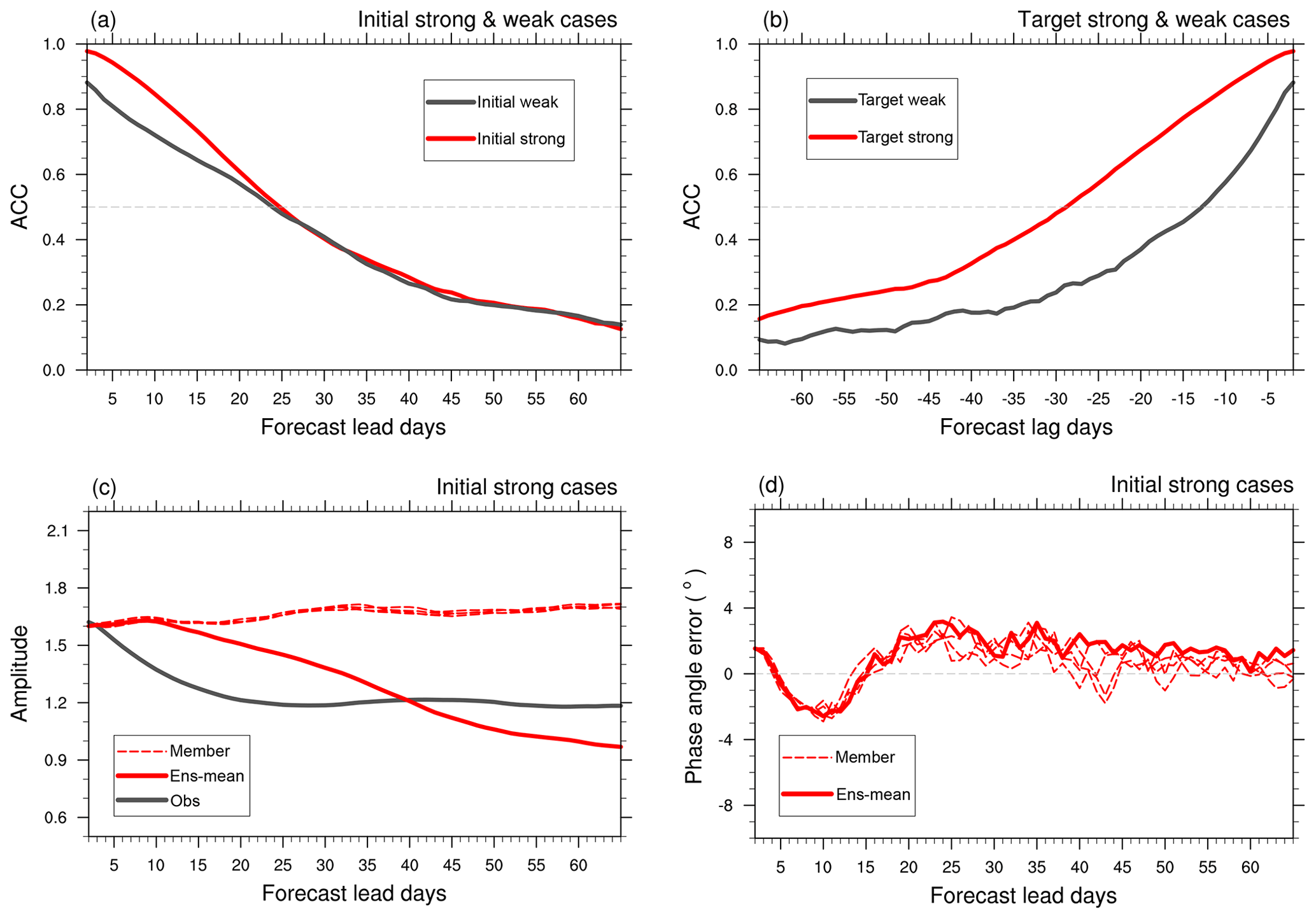
Figure 4 The ACC (a) varied with forecast lead days for initially strong (red) and weak (black) cases and (b) varied with forecast lag days for target strong (red) and weak (black) cases from the ensemble mean. The dashed lines in (a) and (b) have a value of 0.5. (c) The forecast of the MJO amplitude varied with forecast lead days for initially strong cases from the observation (solid black line), individual ensemble members of the model (dashed red line), and their ensemble mean (solid red line). (d) The forecast of the MJO phase angle error (°) for initially strong cases (solid black line). The dashed line in (d) is the reference line with a value of 0.

Increasing the number of ensemble members within a certain range proves to be effective in forecasting the uncertainty in weather and climate (Hou et al., 2001). We employed the time-lagged ensemble method to further augment the ensemble members. The time-lagged ensemble includes the ensemble members generated on the forecast day and from lag times. For instance, by incorporating ensemble members with a lag of i ($i=\mathrm{0},\mathrm{1},\mathrm{2},\mathrm{\dots }$) days, the total number of members becomes $\mathrm{4}\cdot (i+\mathrm{1})$. Upon examining the relationship between lag i days and forecast skill, it was found that the skill increases as i increases at first, but then it reaches a plateau when i>3 (see Fig. A2). This suggests that the forecast skill of the 16 members may represent the limit of the time-lagged ensemble method in IAP-CAS. Figure 3d shows the ensemble of 16 members is more dispersive than that of 4 members, which is illustrated by less distinction between the RMSE and spread in the 16-member system. The ensemble mean of 16 members achieves a skill of 26 d, surpassing the skill of 4 members by 2 d (Fig. 3c).

Numerous prior investigations have demonstrated that MJO forecast skill is sensitive to the MJO amplitude in many models (Lin et al., 2008; Rashid et al., 2011; Wang et al., 2014; Xiang et al., 2022), and this characteristic is also evident in the IAP-CAS model. We classify an MJO case as an initial (target) strong case if its initial (target) amplitude is greater than 1, while an event with an initial (target) amplitude less than 1 is classified as an initial (target) weak case. Figure 4a and b show that in the IAP-CAS model, the forecast skills of strong MJO cases are generally higher than those of weak cases, especially in the target strong (weak) cases.

The amplitude and phase of MJO serve as additional indicators for a detailed assessment of MJO forecast performance. For initially strong MJO cases, we analyze the MJO amplitude and forecasted phase angle error (Fig. 4b and c). The individual member has a stronger amplitude than the observation, which leads to a relatively strong amplitude in the ensemble mean during the initial 40 d. However, as the noise rapidly increases, the phase error of the individual members also escalates (as shown in Fig. 4c). The phase error results in a mutual cancellation in positive and negative phases of MJO among ensemble members, leading to a rapid weakening of the amplitude in the ensemble mean. In Fig. 4d, the phase error of the ensemble mean indicates that the speed of forecasted MJO tends to decrease at first and then starts increasing around the 10th day. A more detailed investigation into the speed of propagating MJO events is described in Sect. 5.

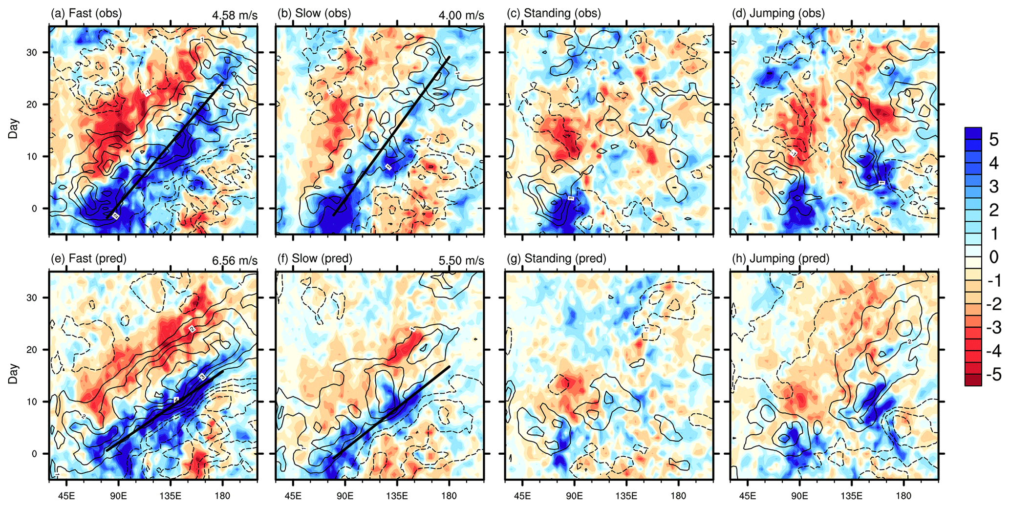
Figure 5 The 10° S–10° N averaged precipitation anomalies (shading; mm d⁻¹) and 850 hPa zonal wind anomalies (contours with an interval of 1 m s⁻¹), varied with longitude (x axis) and time lag (y axis; days), composited for four types of the boreal winter MJO. Panels (a)–(d) are for the observation (NCEP winds and GPCP precipitation), and panels (e)–(h) are for model forecasts. The thin solid black lines represent positive values, and the dashed lines represent negative values. The thick solid black line represents the propagation trajectory of the MJO, derived via least squares regression. The propagation speed of the propagating MJO is annotated in the top-right corner of the panels.

5 The forecast of MJO propagation

We present a qualitative diagnostic of a 20-year hindcast experiment to evaluate the overall forecast skills of IAP-CAS in Sect. 4. This analysis provides us with preliminary insights into the performance and biases of the system. Given that the MJO is more pronounced during boreal winter, our focus is concentrated from November to the following April. Based on Wang et al. (2019), we aim to conduct further investigations into different types of boreal winter MJO events to explore the physical explanation of system biases.

In Sect. 3, we describe the methodology for classifying MJO events and results. Figure 5 compares the composited propagation patterns of precipitation and U850 between the observation and forecast for four different MJO types. In observations, the fast-propagating MJO (Fig. 5a) and slow-propagating MJO (Fig. 5b) exhibit a consecutive eastward propagation structure from the Indian Ocean across the MC region to the Pacific Ocean. The primary distinction between the two types lies in their propagation speed. The fast-propagating MJO demonstrates a faster speed, with a velocity of 4.58 m s⁻¹, compared to the slow-propagating type, which moves at 4 m s⁻¹. The standing MJO (Fig. 5c) remains relatively stationary over the Indian Ocean and does not continue to propagate eastward. The jumping MJO (Fig. 5d) shows a convective system that bypasses the MC region and directly jumps from the Indian Ocean to the Pacific Ocean. Here, fast MJO and slow MJO are considered propagating MJO events, while the latter two types are regarded as non-propagating MJO events.

The observed U850 displays a coupled structure characterized by equatorial westerly anomalies of the Kelvin wave component located west of the convection and easterly anomalies of the Rossby wave component located east of the convection (Rui and Wang, 1990; Adames and Wallace, 2014; Wang and Lee, 2017). As illustrated in Fig. 5, a distinct contrast between propagating MJO and non-propagating MJO can be found in the circulation at the low level: in the propagating MJO events, the Kelvin wave response is strong and tightly coupled with the center of convection, which is shown in the stronger and eastward-extending easterly wind component, particularly prominent in fast MJO events. Many previous studies (Benedict and Randall, 2007; Hsu and Li, 2012; Wang and Lee, 2017) have also indicated that the presence of low-level easterly winds is a key signal that contributes to the eastward propagation of MJO by inducing low-level convergence and premoistening to the east of the major convection. In the non-propagating MJO events, the easterly wind is weak and tends to decouple from the major convection.

The model accurately reproduces the propagating morphology of the MJO and exhibits coupled signals of Kelvin and Rossby waves (Fig. 5e and f). However, a noticeable acceleration in speed is evident, particularly in the case of fast MJO, reaching speeds of 6 m s⁻¹, while the simulated slow MJO moves at 5 m s⁻¹. Figure 5g also shows that the forecast for standing MJO remains somewhat imprecise. This aspect is also evident in the MJO forecast skill depicted in Fig. 6, where the standing MJO has the lowest skill (13 d). For each MJO type, we consider the skill as the ACC of the cases initiated from day −20 to day 15 (Xiang et al., 2015). Figure 6 shows that the fast MJO achieves the highest skill at 32 d, while the jumping MJO and slow MJO exhibit skills of 23 and 21 d, respectively.

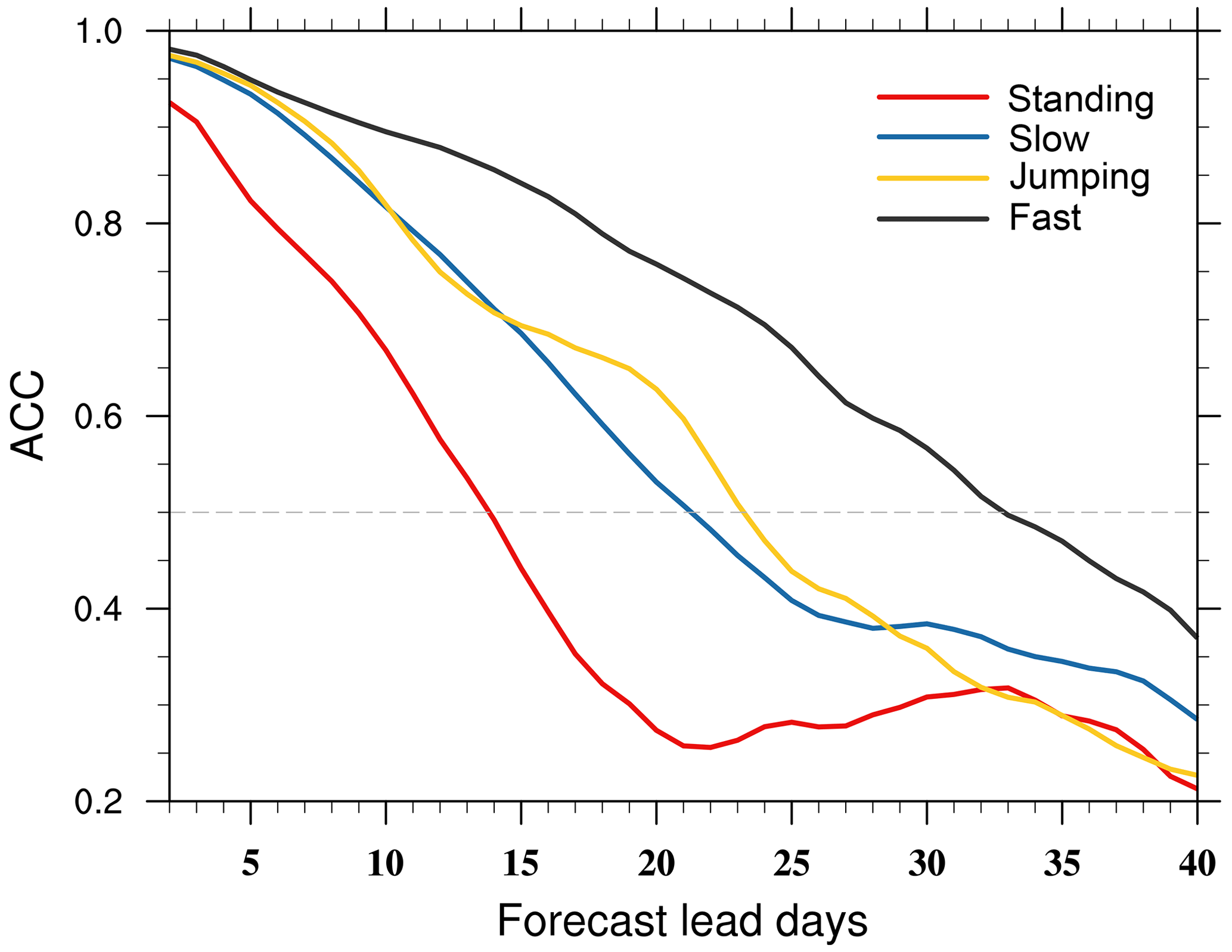
Figure 6 The bivariate ACC as a function of forecast lead days for fast, slow, jumping, and standing MJO events. The dashed line has a value of 0.5.

Additionally, from the Hovmöller diagram of observed propagating MJO (Fig. 5a and b), a significant change in convection is observed after crossing the MC region, which is marked by a decrease in intensity and a slower propagation speed. This change is roughly delineated by 135° E, which is commonly referred to as the MC barrier. As mentioned above, the MC barrier effect is usually amplified in climate models. In the IAP-CAS model, the forecasted convective signal of slow MJO appears to stop after crossing the MC region. Could this indicate an amplification of the MC barrier issue in the IAP-CAS model? However, this phenomenon is less pronounced in the simulation of fast MJO. Due to the zonal averaging in the Hovmöller diagram, some information may be obscured. Further investigation is required to determine the detailed characteristics of the propagating MJO simulated by the model.

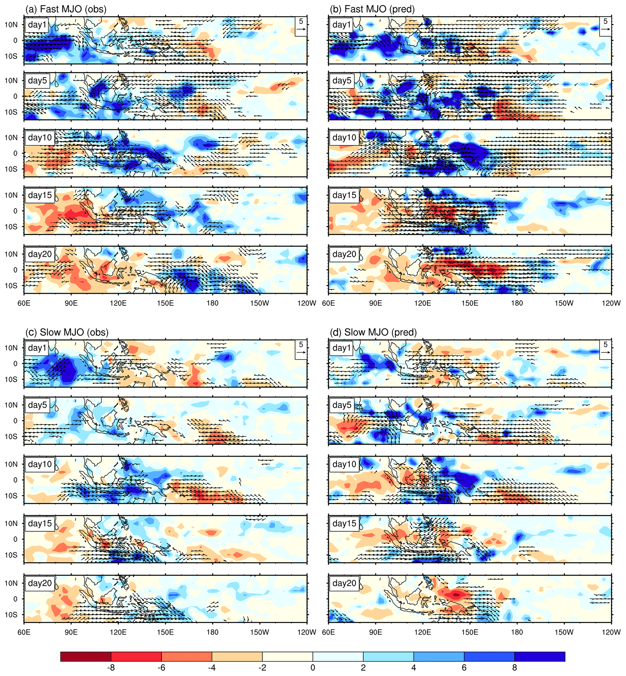
Figure 7 Evolution patterns of the composite precipitation (shading; mm d⁻¹) and 850hPa winds (vectors; m s⁻¹) anomalies (exceeding 2 m s⁻¹) for day 1, day 5, day 10, day 15, and day 20 in (a) observed fast MJO, (b) simulated fast MJO, (c) observed slow MJO and (d) simulated slow MJO.

Figure 7 presents the evolution patterns of propagating MJO. In the first 10 d, it is noticeable that the forecasted precipitation intensity of propagating MJO is significantly higher than observed, especially in the case of fast MJO. Coupled winds in 850 hPa also exhibit stronger magnitudes, with a larger zonal scale. The forecasted location of the major convection is relatively biased towards the east, which further confirms that there is an overestimation of the propagation speed. On the 15th day, the MJO convective system crosses the MC region and reaches the eastern Pacific. It is worth noting that the forecasted negative phase of MJO exhibits a significant development, with an accelerated speed, gradually intruding into the positive phase (Fig. 7b and d). By the 20th day, the development of the negative phase has further intensified, extending its influence into the tropical eastern Pacific region, while in the observation, the negative phase remains east of the MC region. In the later stages, as the negative phase intrudes, the forecasted convective signal in the positive phase is almost absent due to the inherently weaker convection in slow MJO. The disappearance of the slow MJO signal observed in the Hovmöller diagram after crossing the MC region may stem from the intrusion of the negative phase. This might differ from the commonly defined issue of MC barrier amplification observed in many models.

In Fig. A3, simulations also show that both standing MJO and jumping MJO exhibit overall enhanced convective intensity. However, they accurately capture the non-propagating characteristics of the observed MJO, such as the weak coupling of Kelvin waves and the strong coupling of Rossby waves.

6 The possible physical explanation for the forecast biases

Section 5 highlights some biases observed in the forecast of propagating MJO, which include stronger amplitude and faster propagation speed in the IAP-CAS model. These biases are also mentioned in Sect. 4. In this section, we aim to unravel the physical mechanisms underlying these biases.

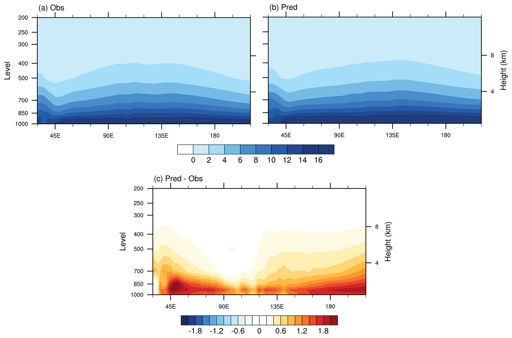
Figure 8 The longitude–vertical profiles of winter (November–April) mean specific humidity (g kg⁻¹) averaged over 10° S–10° N for (a) the observation, (b) the IAP-CAS model, and (c) the difference between the IAP-CAS model and observation.

As a large-scale convective system, MJO's genesis, evolution, and dissipation are intricately linked to atmospheric moisture (Wang, 1988; Kemball-Cook and Weare, 2001; Maloney, 2002; Wang and Lee, 2017). Given that the model forecasts exhibit a systematic bias of stronger amplitude, we start with the diagnosis of the background state in moisture. Figure 8 shows the winter mean specific humidity averaged over 10° S–10° N. A clear positive bias of the background moisture state in the IAP-CAS model is observed (Fig. 8c), which can enhance the convection in the MJO. However, the distribution of this moisture bias is non-uniform. Figure 8c illustrates that the positive moisture bias is more pronounced towards the western Indian Ocean and the central-eastern Pacific, and this bias gradually spreads to the upper levels. However, in the MC region, the positive moisture bias is smaller and primarily concentrated in the low level. We speculate that higher evaporation fluxes in the model may be the reason for the positive moisture bias. Therefore, the reduction in oceanic surface area within the MC region contributes to a decrease in this positive bias.

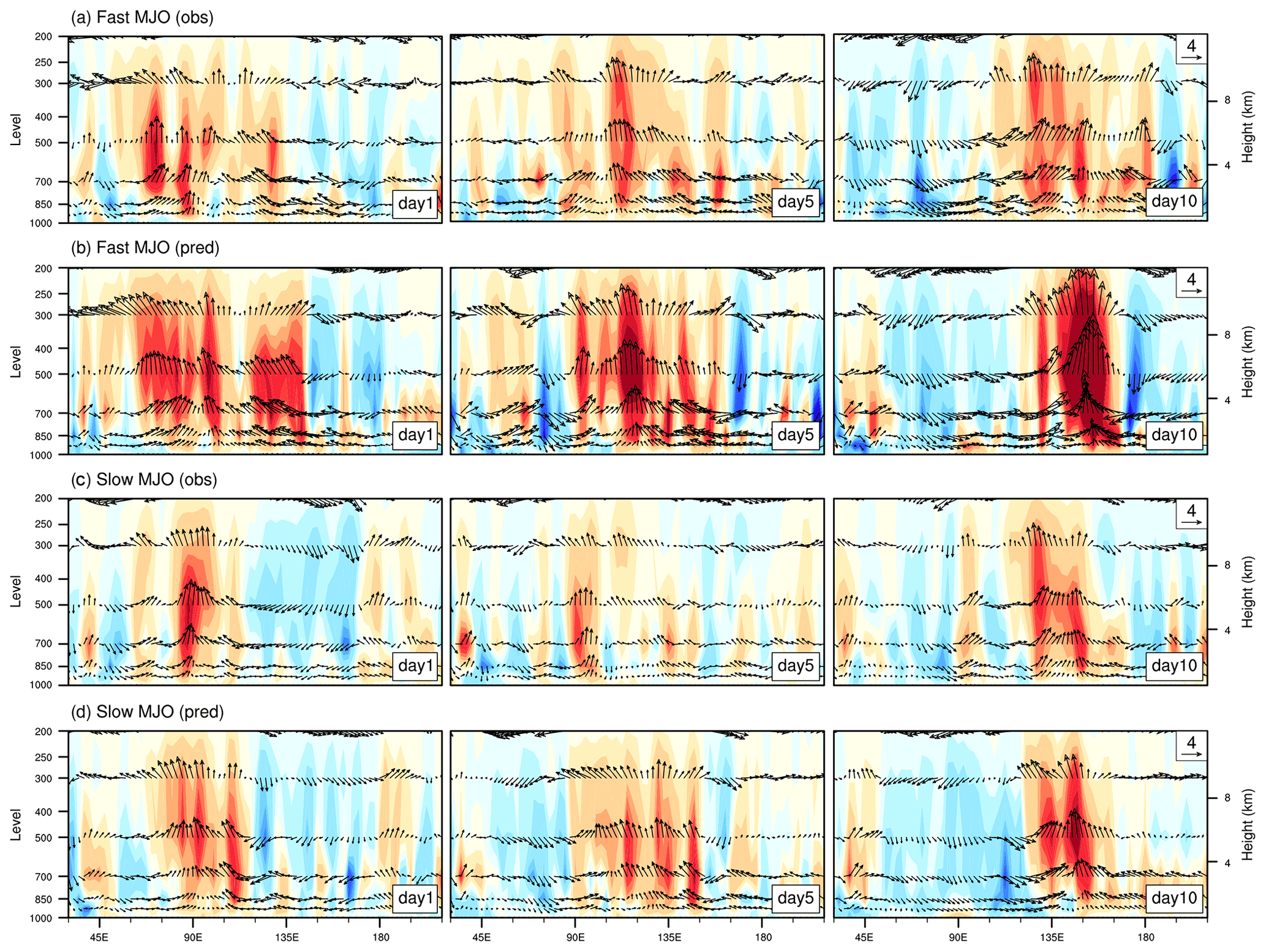
Figure 9 The composited longitude–vertical structure of precipitation heating (contours; 1 × 10⁻² $\mathrm{J}{\mathrm{kg}}^{-\mathrm{1}}{\mathrm{s}}^{-\mathrm{1}}$) and zonal and vertical wind anomalies (vectors; units are m s⁻¹ for zonal winds and 0.01 Pa s⁻¹ for vertical winds) averaged over 10° S–10° N for day 1, day 5, and day 10 in (a) observed fast MJO, (b) simulated fast MJO, (c) observed slow MJO, and (b) simulated slow MJO.

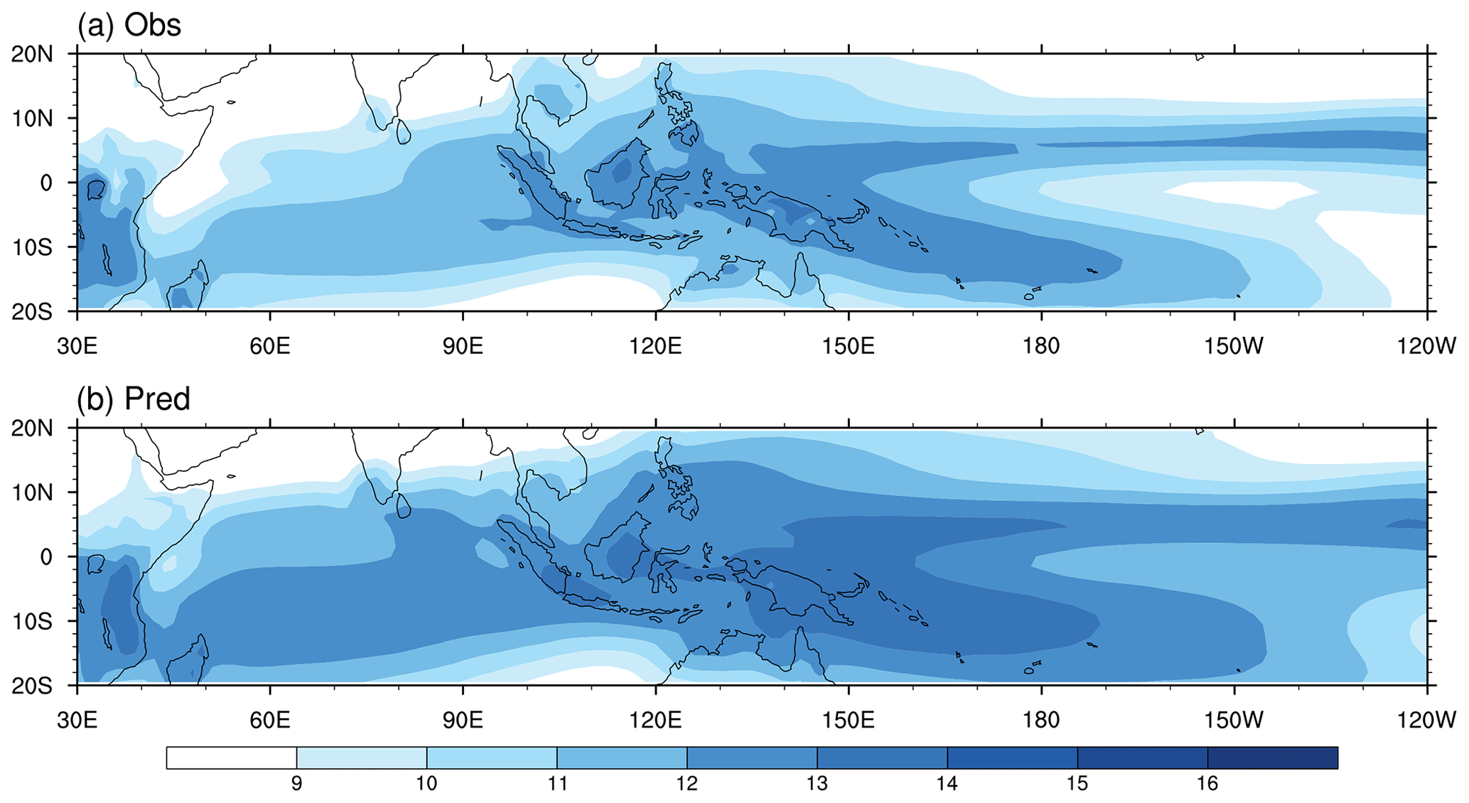
Figure 10 Winter (November–April) mean specific humidity (g kg⁻¹) on 850 hPa for the (a) observation and (b) IAP-CAS model.

Figure 9 displays the precipitation-induced condensational heating (Q₂) during fast MJO and slow MJO events. The condensational heating serves as a proxy for the distribution of convection, which was estimated by the moisture sink defined as

$$\begin{array}{}\text{(11)}& Q_{\mathrm{2}}=-L_{\mathrm{v}}\left({\displaystyle \frac{\partial q}{\partial t}}+\mathit{V}\cdot \mathrm{\nabla }q+\mathit{\omega }{\displaystyle \frac{\partial q}{\partial p}}\right),\end{array}$$

where q is the specific humidity; V is the horizontal circulation; ω is the vertical pressure velocity; and L_v is the latent heat at condensation, which is a constant here. The vertical distribution of Q₂ reveals that both fast MJO and slow MJO events in the model forecasts trigger stronger convection, particularly in the fast MJO events. Furthermore, the enhanced convective heating leads to a strong response in the coupled-MJO-related circulation (Fig. 9). From the 1st day to the 10th day, there is a gradual strengthening process observed in the simulated convection, particularly pronounced in the fast MJO, with its intensity peaking on the 10th day.

To further understand the propagation and intensity variations in MJO in the IAP-CAS model, it is necessary to comprehend the underlying physical processes associated with it. Under the framework of the moisture mode, Jiang (2017) performed a moisture budget analysis on the latest generation of general circulation models (GCMs) and identified the key processes for the eastward propagation of MJO. This research revealed that the advection (${\mathit{V}}^{\prime }\cdot \mathrm{\nabla }\stackrel{\mathrm{‾}}{Q}$) of the seasonal mean moisture ($\stackrel{\mathrm{‾}}{Q}$) by the MJO anomalous circulations (V^′) plays a crucial role in the propagation of MJO. By increasing moisture eastward and decreasing it westward of the MJO convection, the advection regulates the propagation. (D. Kim et al., 2014; Adames and Kim, 2016; Jiang et al., 2018). Among the two determining factors (V^′ and $\stackrel{\mathrm{‾}}{Q}$), the role of the moisture gradient term is further emphasized. Many studies (Gonzalez and Jiang, 2017; DeMott et al., 2018; Ahn et al., 2020) have demonstrated that the mean moisture's horizontal gradient plays a crucial role in determining the propagation of MJO (Fig. 10a). It is well forecasted in the models that simulate MJO well, leading to realistic horizontal mean moisture gradients and, thus, well-forecasted horizontal moisture advection associated with the MJO (Hsu and Li, 2012; D. Kim et al., 2014; Nasuno et al., 2015; Adames and Wallace, 2015; Gonzalez and Jiang, 2017). The IAP-CAS model is capable of reproducing this gradient, although there is an overall stronger moisture bias (Fig. 10b). Here, the $\stackrel{\mathrm{‾}}{Q}$ presented is the winter mean specific humidity at 850 hPa (${\stackrel{\mathrm{‾}}{Q}}_{\mathrm{850}}$). Research has indicated that ${\stackrel{\mathrm{‾}}{Q}}_{\mathrm{850}}$ is representative (Kim, 2019), and subsequent analysis also focuses on the 850 hPa level.

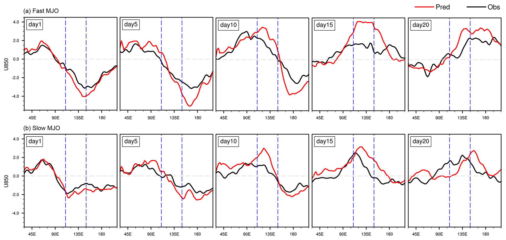
Figure 11 The composited longitudinal structure of the 850 hPa zonal wind anomalies (m s⁻¹) averaged over 15° S–15° N for day 1, day 5, day 10, day 15, and day 20 from the observation (solid black line) and IAP-CAS model (solid red line) in fast and slow MJO events. The dashed gray line is the reference line with a value of 0. The two dashed blue lines are 110 and 150° E, respectively, which denote the extension of the MC region.

Figure 11 shows the composite equatorial U850 anomalies averaged over 15° S–15° N for fast MJO and slow MJO, respectively, and depicts the transition from westerly to easterly winds in the MC region (as enclosed by the two dashed blue lines), leading to the change from positive advection to negative advection. On the 1st and 5th days, the MC region is predominantly occupied by easterly winds, while from the 10th to the 20th day, the region is primarily characterized by westerly winds in both fast MJO and slow MJO. However, the forecasted amplitude of low-level wind is significantly stronger, which can be caused by the enhanced MJO convection as explained earlier.

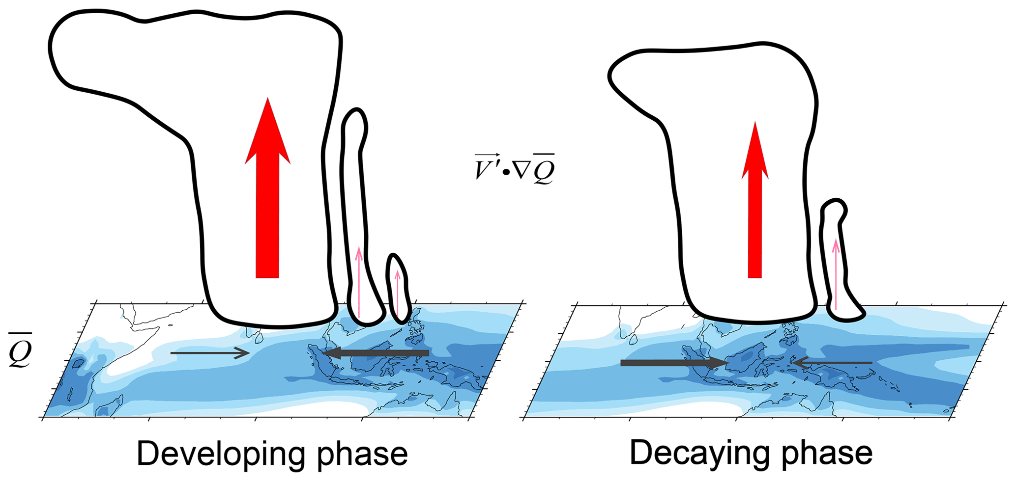
Figure 12 Schematic diagrams illustrating the moisture mode theory on MJO propagation in the MC region.

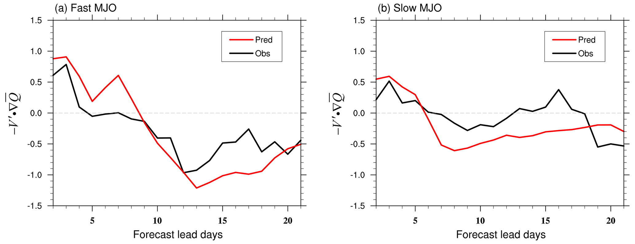
Figure 13 The composited $-V^{\prime }\cdot \mathrm{\nabla }\stackrel{\mathrm{‾}}{Q}$ ($\mathrm{g}{\mathrm{kg}}^{-\mathrm{1}}{\mathrm{s}}^{-\mathrm{1}}$) averaged over the MC region (15° S–15° N, 110–150° E) as a function of forecast lead days from the observation (solid black line) and IAP-CAS model (solid red line) in (a) fast MJO and (b) slow MJO events. The dashed gray line is the reference line with a value of 0.

The MJO anomalous circulation patterns in the MC region result in a positive moisture advection on the eastern part of the MJO during the early stages of the MJO's development, which facilitates the propagation of convection in the positive phase. We refer to this process as the “developing phase”. Figure 12 provides a detailed illustration of this process. Conversely, during the later stages, there is a negative moisture advection on the western side of the MJO, which leads to the propagation of convection in the negative phase and promotes the dissipation of the MJO. We refer to this process as the “decaying phase” (Fig. 12). Compared to the observation, the stronger amplitude of the low-level moisture advection (${\mathit{V}}^{\prime }\cdot \mathrm{\nabla }\stackrel{\mathrm{‾}}{Q}$) in the model explains the gradual enhancement of convective moist phases during the early stages and the amplification of convective dry phases during the later stages (Fig. 13). The model's moist environment leads to intensified convection, triggering the strengthening of coupled wind fields, which in turn enhances the moist phase in the early stage and the dry phase in the later stage of convection. Consequently, during the development phase of the MJO, its amplitude gradually strengthens. Conversely, during the decaying phase of the MJO, the intensity of the dry phase also progressively increases.

As the simulated propagating MJO gradually intensifies, we observe an enhancement of easterly winds on the east of the convective center, accompanied by an overestimation in zonal scale, indicating the triggering of stronger Kelvin waves (Fig. 7b and d). According to Wang et al. (2019), MJO with a larger zonal scale will experience an increased eastward propagation speed since the phase speed is inversely proportional to the wave number. This phenomenon is also observed in the observation, where the Kelvin wave response to fast MJO exhibits a larger zonal scale compared to slow MJO. Subsequently, during the decay phase of the propagating MJO, the model exhibits a pronounced Rossby wave response triggered by the MJO, leading to the intrusion of convective negative phases and facilitating the dissipation of the MJO.

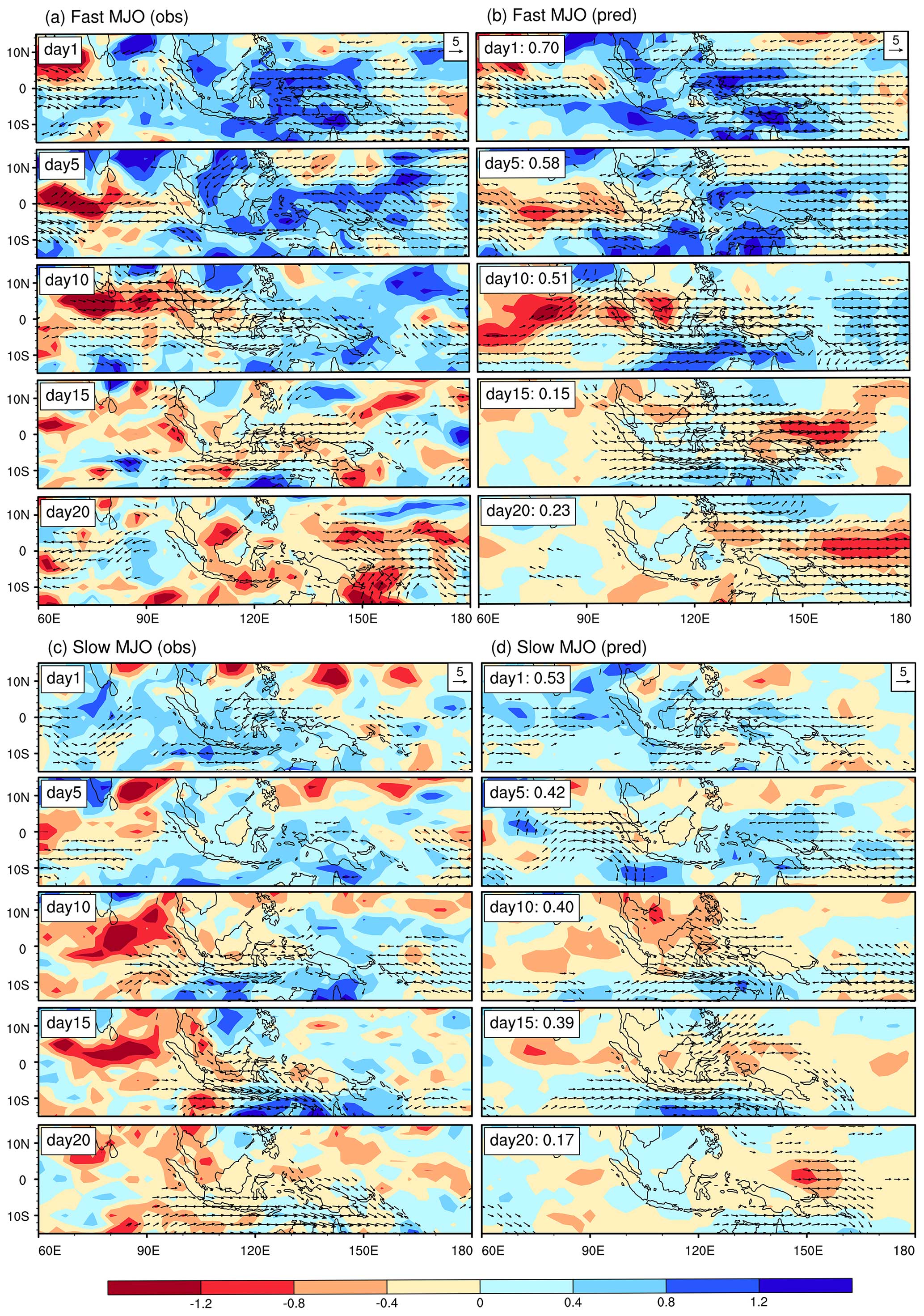
Figure 14 Evolution patterns of the composite specific humidity anomalies (g kg⁻¹) and wind (vectors; m s⁻¹) anomalies (exceeding 2 m s⁻¹) on 850 hPa for day 1, day 5, day 10, day 15, and day 20 (a) observed fast MJO, (b) simulated fast MJO, (c) observed slow MJO, and (b) simulated slow MJO. The spatial correlation coefficient between the simulated and observed moisture anomalies is shown to the right of panels (b) and (c).

In addition to examining the winter mean moisture state ($\stackrel{\mathrm{‾}}{Q}$), we analyzed MJO-related moisture anomalies (Q^′) as well (Fig. 14). By comparing the evolution pattern of moisture anomalies between slow MJO and fast MJO, it is found that the moisture anomalies in the eastern part of fast MJO are more intense compared to the slow MJO. This results in stronger low-level moisture transport towards the convective region, thereby also facilitating the intensification and acceleration of the MJO. Moreover, there is a significant distinction in the spatial correlation between fast and slow MJO, and it happens as early as the first day. As the forecast lead time progresses, the accuracy of the moisture forecast deteriorates, while fast MJO events display comparatively better performance. The disparity in moisture anomalies is possibly a pivotal factor contributing to differences in forecast skills between the fast (32 d) and the slow MJO (21 d). This underscores the significance of improving moisture forecast in the MJO forecast.

7 Summary and discussion

7.1 Summary

The graphical abstract presents a workflow for this paper, outlining the structure of this work. This study introduces a newly developed S2S ensemble forecast system of the IAP-CAS model. The introduction primarily focuses on the numerical model, initialization, ensemble generation, and post-processing aspects of the S2S system. Then we aim to identify potential possibilities for developing this S2S system through a comprehensive assessment of its forecast skills. Based on the 20-year hindcast experiment, the IAP-CAS model shows comparable skill (24 d) to other S2S models. However, the ensemble forecast for MJO has been demonstrated to be underdispersive. A detailed examination of the propagating MJO forecasted in the IAP-CAS model reveals that the amplitude of the convection is overestimated with an increasing propagation speed, particularly in the fast MJO events. These biases are accompanied by a faster dissipation of the MJO.

The root cause of these biases lies in the model's wetter environment, which leads to enhanced convection and strengthened circulation coupled with convection. This, in turn, further amplifies convection during the development of propagating MJO. The gradual intensification of MJO strength and coupled Kelvin waves is mainly associated with the stronger amplitude of the low-level moisture advection (${\mathit{V}}^{\prime }\cdot \mathrm{\nabla }\stackrel{\mathrm{‾}}{Q}$) in the forecast. The overestimate in the zonal scale of Kelvin waves accelerates the propagation of the propagating MJO in the model. Similarly, the strengthening of Rossby waves also hastens the dissipation of the MJO. Moreover, the differences in forecast skills between the fast MJO and the slow MJO may be attributed to discrepancies in moisture anomaly (Q^′) forecast. This further underscores the significance of accurate moisture forecasts.

7.2 Discussion

In Fig. A4, we compare the forecast skill of the IAP-CAS model with 11 other S2S models. The MJO index of 12 S2S models and ERA-Interim from the S2S website (http://www.s2sprediction.net/, last access: 1 December 2023) is used for evaluation during the standard hindcast period of 2001–2010. In Fig. A4, we observe improved forecast skill in ensemble forecasts compared to deterministic forecasts. Among the 12 S2S models, the IAP-CAS model exhibits MJO skill above the mean skill level, while the ECMWF model stands out as the highest-performing model. Figure A5a shows that the skill of individual members in ECMWF is approximately 17–18 d, whereas the ensemble mean demonstrates an extended skill of up to 30 d. This phenomenon may be attributed to the ECMWF model's considerable dispersion (Fig. A5b), which once again underscores the critical role of ensemble dispersion in forecasting uncertainties in weather and climate.

Therefore, the forthcoming phase in our model's development plan encompasses increasing model dispersion through improved ensemble perturbation methods, with the ultimate goal of improving model forecast skills. The method of orthogonal conditional nonlinear optimal perturbations (CNOPs; Mu et al., 2003) and the second-order exact sampling (Pham, 2001) are both promising approaches for generating initial perturbations in the model. This method allows the generation of a set of initial perturbations in different orthogonal perturbation subspaces, each with the maximum potential for nonlinear development. When applied to ensemble forecast using a simple Lorenz 96 model, the CNOPs method has demonstrated higher forecast skill compared to the commonly used linear singular vector (SV) method (Mureau et al., 1993). Furthermore, the Parallel Data Assimilation Framework (PDAF; Nerger et al., 2020) provides an efficient method known as second-order exact sampling, which uses the long-time variability of the model dynamics to estimate the uncertainty. Evidence has already suggested that the use of second-order exact sampling can greatly improve the skill in sea ice extent throughout the Arctic and along the Northern Sea Route (Yang et al., 2020). We plan to explore the application of CNOPs and second-order exact sampling in the IAP-CAS model in the future and eagerly anticipate the potentially significant results it may yield. Additionally, using machine learning to improve the skill of ensemble forecast is also a viable way to enhance the ensemble forecast of our model.

In addition to exploring ensemble perturbations, we also intend to enhance the initialization system of the model. Recognizing the moisture and acknowledging the issue of moisture bias in the IAP-CAS model are crucial in the forecast of MJO; it is essential to take measures to ameliorate moisture forecast in our model. Recent research by Zeng et al. (2023) provides convincing evidence that humidity initialization can indeed significantly enhance MJO forecast in the IAP-CAS S2S forecast system, especially in the second and third phases of MJO propagation. However, it is worth noting that changes in the mean state have a significant impact on MJO development (Hannah et al., 2015; Kim, 2019). We must thus pay attention to the influence of moisture initialization on the mean state. Moreover, the current S2S system's initialization process uses the nudging method, and it is worthwhile to explore more efficient methods to enhance the initialization process.

We are also considering increasing the resolution of the model to C384 (25 km) globally. A high-resolution coupled model could better represent the MJO (Crueger et al., 2013). This improvement could be attributed to the enhanced resolution, which better captures the ocean–atmosphere interaction – a critical factor for MJO convection. Increasing the resolution is also meaningful for enhancing forecasts in the MC region by accurately depicting terrain distortion (Hsu and Lee, 2005; Inness and Slingo, 2006; Wu and Hsu, 2009). Further optimizing the model's physical processes and dynamic–physical coupling is also believed to enhance the forecast of the MJO (Zhou and Harris, 2022). As the foreseeable resolution and complexity of the model increase in the future, the issue of power consumption on X86 architecture processors for handling the growing amount of data will become more pronounced. We have plans to port the model to the computing platform based on ARM architecture to address the challenges posed by the explosive growth of data.

Appendix A

Table A1 Hybrid coefficient of hybrid sigma-pressure coordinates at layer interfaces in CAS FGOALS-f2.

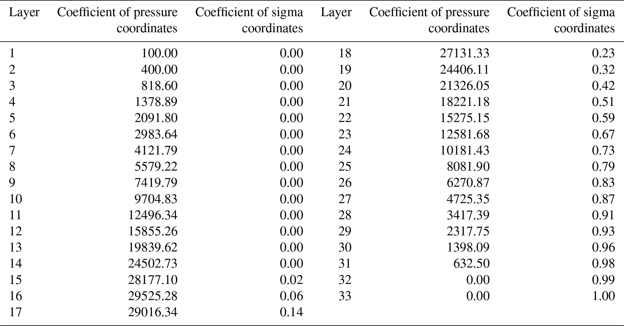
Table A2 Initialization information of the S2S ensemble forecast system.

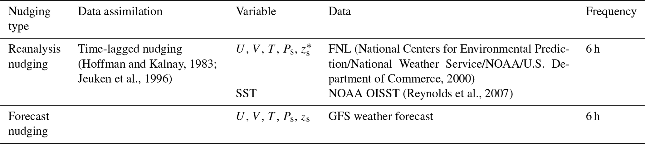
^∗ Table notes: U represents zonal wind, V represents meridional wind, T represents temperature, P_s represents surface pressure, z_s represents surface geopotential height, and SST represents sea surface temperature.

Table A3 Introduction to the output data of the S2S ensemble forecast system.

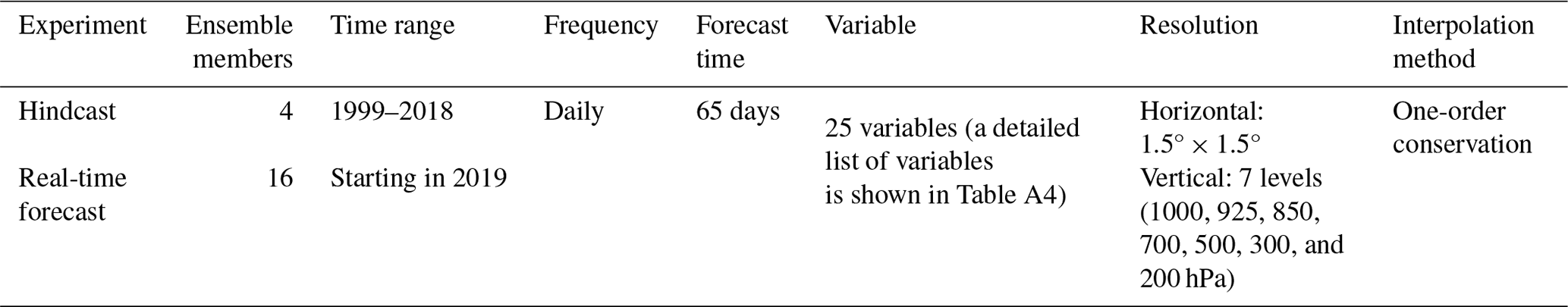
Table A4 List the output variables in the S2S ensemble forecast system.

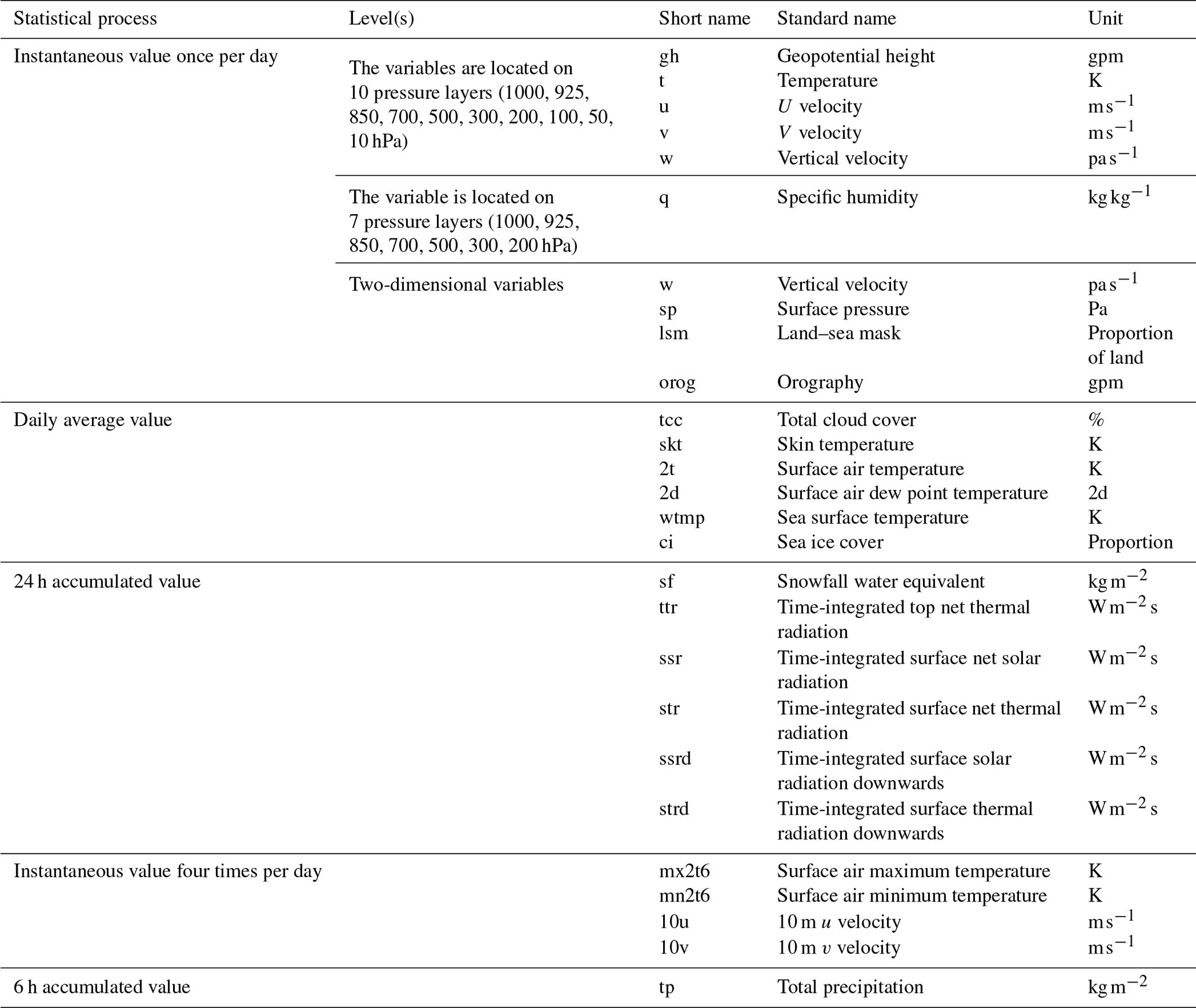
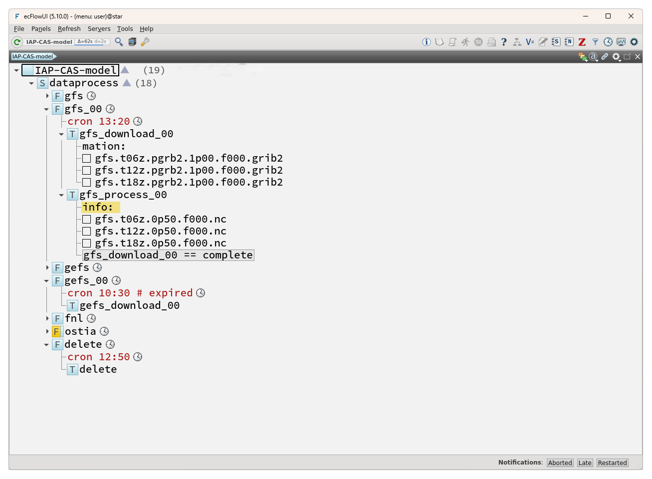
Figure A1 The structure of ecFlow (ECMWF workflow). ecFlow, developed and maintained by the ECMWF, is a client–server workflow package designed to facilitate the execution of a substantial number of programs within a controlled environment. ©European Centre for Medium-Range Weather Forecasts (ECMWF), 2005. It is used in the IAP-CAS model to accomplish the download and preprocessing of the forcing data.

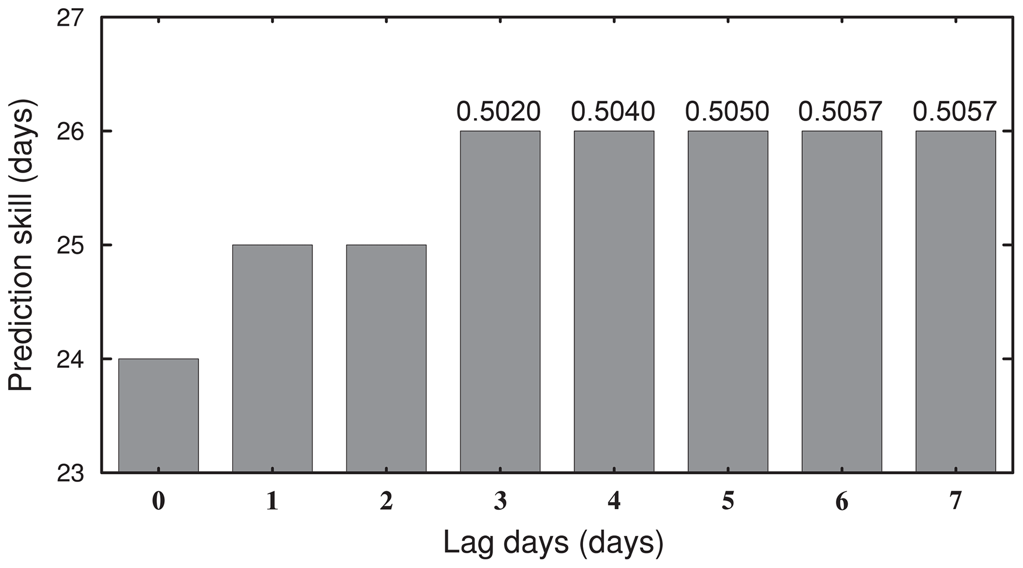
Figure A2 MJO forecast skill of the ensemble mean of time-lagged members as a function of lag days. The values on the bars represent the ACC on day 26.

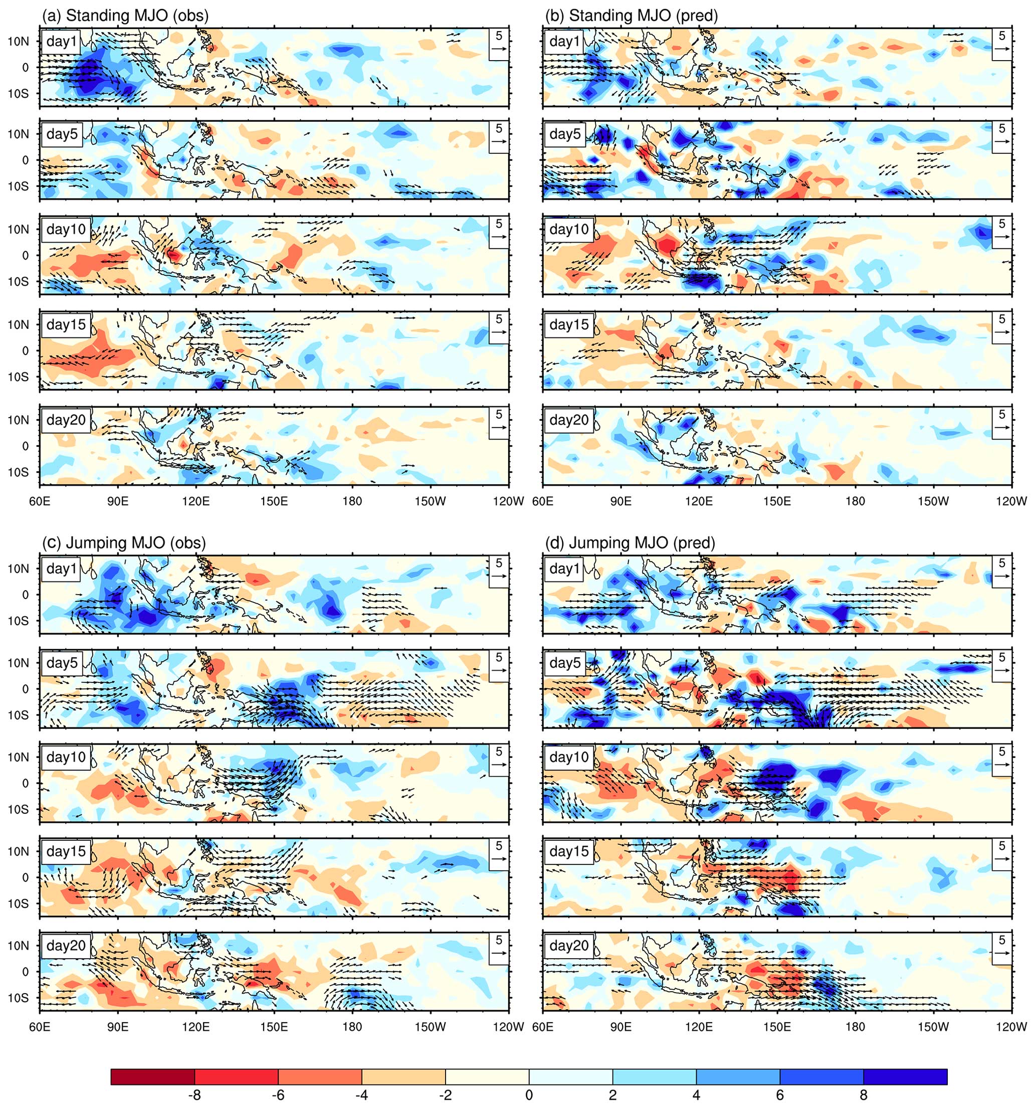
Figure A3 Evolution patterns of the composite precipitation (shading; mm d⁻¹) and 850hPa wind (vectors; m s⁻¹) anomalies (exceeding 2 m s⁻¹) for day 1, day 5, day 10, day 15, and day 20 in (a) observed standing MJO, (b) simulated standing MJO, (c) observed jumping MJO, and (d) simulated jumping MJO.

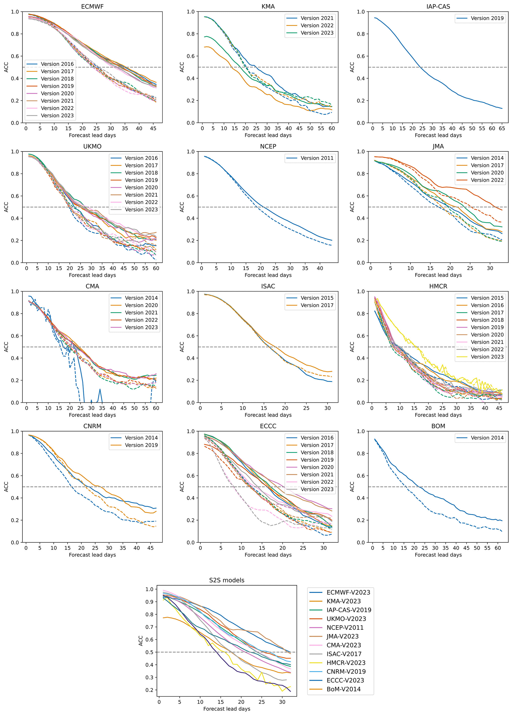
Figure A4 The MJO forecast skill of 12 S2S models, providing comparisons between various model versions over the years, and the latest versions of 12 models. The evaluation covers the period from 2001 to 2010, except for CMA, which spans 2008 to 2013. The solid lines represent the skill of ensemble mean forecasts, while the dashed lines represent the skill of deterministic forecasts.

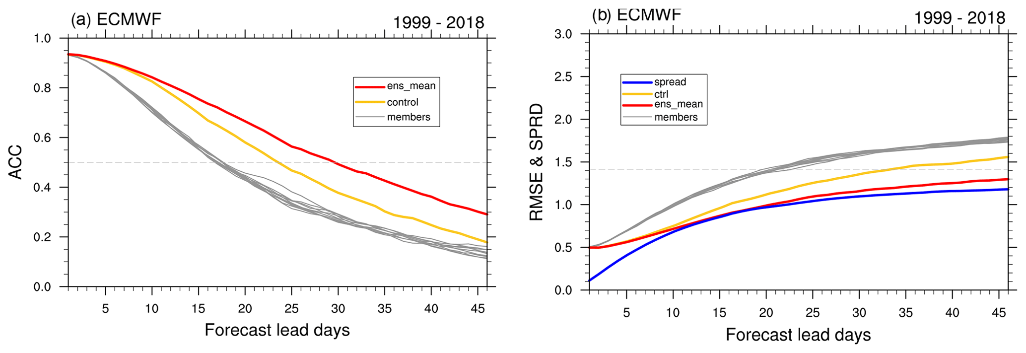
Figure A5 The ACC (a) and the RMSE (b) of ECMWF (2019 version) from individual members (solid gray line), ensemble ctrl (solid yellow line), and 10-member ensemble mean (solid red line) as a function of forecast lead days. The solid blue line denotes the ensemble spread. The dashed line in (a) has a value of 0.5, and it represents 1.414 in (b).