Islet: interpolation semi-Lagrangian element-based transport

Advection of trace species, or tracers, also called tracer transport, in models of the atmosphere and other physical domains is an important and potentially computationally expensive part of a model's dynamical core. Semi-Lagrangian (SL) advection methods are efficient because they permit a time step much larger than the advective stability limit for explicit Eulerian methods without requiring the solution of a globally coupled system of equations as implicit Eulerian methods do. Thus, to reduce the computational expense of tracer transport, dynamical cores often use SL methods to advect tracers. The class of interpolation semi-Lagrangian (ISL) methods contains potentially extremely efficient SL methods. We describe a finite-element ISL transport method that we call the interpolation semi-Lagrangian element-based transport (Islet) method, such as for use with atmosphere models discretized using the spectral element method. The Islet method uses three grids that share an element grid: a dynamics grid supporting, for example, the Gauss–Legendre–Lobatto basis of degree three; a physics parameterizations grid with a configurable number of finite-volume subcells per element; and a tracer grid supporting use of Islet bases with particular basis again configurable. This method provides extremely accurate tracer transport and excellent diagnostic values in a number of verification problems.

1 Introduction

An atmosphere model has two parts: the dynamical core, which computes resolved fluid flow and resolved thermodynamics (Lauritzen, 2011); and the subgrid parameterizations, which compute unresolved chemistry and physics processes (Stensrud, 2009). In turn, the dynamical core also has two parts: first, the dynamics solver, which solves the equations of fluid motion; second, the tracer transport solver, which advects trace atmosphere species, or tracers, using the air density and flow fields from the dynamics solver.

Because of the large number of tracers in climate models, tracer transport can be computationally very expensive. For example, in the Dept. of Energy's Energy Exascale Earth System Model (E3SM) (E3SM Project, 2018) Atmosphere Model (EAM) version 1 (Golaz et al., 2019), configured with the default 40 tracers, tracer transport takes approximately 75 % of the total dynamical core wall clock time and approximately 23 % of the total atmosphere model wall clock time on a typical computer cluster (Golaz et al., 2022, Fig. 3). For EAM version 2, we developed a new tracer transport method that is 6.5 to over 8 times faster than in EAM version 1 in the cases of, respectively, low and high workload per computer node (Golaz et al., 2022, Fig. 3). In addition, we developed remap operators to remap data between separate grids for physics parameterizations and dynamics, permitting the physics parameterization computations to run on a coarser grid and thus 1.6 to 2.2 times faster in version 2 than in version 1 (Hannah et al., 2021; Golaz et al., 2022).

In this article, we describe the interpolation semi-Lagrangian element-based transport method, with the acronym stylized as “Islet” rather than “ISLET” to minimize distracting all-capitalized text. The Islet method extends those we developed for EAM version 2 by providing the discretizations with natural parameters to trade between computational cost and accuracy in tracer transport and physics parameterizations for a given, fixed dynamical core configuration.

1.1 Problem statement

The mass continuity equation for the air density ρ is

$$\begin{array}{}\text{(1)}& {\displaystyle \frac{\partial \mathit{\rho }}{\partial t}}+\mathrm{\nabla }\cdot \left(\mathit{\rho }\mathit{u}\right)=\mathrm{0},\end{array}$$

where u is the flow velocity. The tracer transport equation in continuity form and with a source term for a tracer mixing ratio q and corresponding tracer density ρq is

$$\begin{array}{}\text{(2)}& {\displaystyle \frac{\partial \left(\mathit{\rho }q\right)}{\partial t}}+\mathrm{\nabla }\cdot \left(\mathit{\rho }q\mathit{u}\right)=\mathit{\rho }f,\end{array}$$

where f is a source term for q. Combining Eqs. (1) and (2) gives the advective form of the tracer transport equation,

$$\begin{array}{}\text{(3)}& {\displaystyle \frac{\mathrm{D}q}{\mathrm{D}t}}\equiv {\displaystyle \frac{\partial q}{\partial t}}+\mathit{u}\cdot \mathrm{\nabla }q=f.\end{array}$$

Because of time splitting in the atmosphere model, our focus is often on the sourceless advection equation,

$$\begin{array}{}\text{(4)}& {\displaystyle \frac{\mathrm{D}q}{\mathrm{D}t}}=\mathrm{0}.\end{array}$$

At position x and time t₁, the exact solution of Eq. (4) in terms of the solution at another time t₀ is

$$\begin{array}{}\text{(5)}& q(\mathit{x},t_{\mathrm{1}})=q\left(\mathit{X}\right(t_{\mathrm{0}};\mathit{x},t_{\mathrm{1}}),t_{\mathrm{0}}).\end{array}$$

$\mathit{X}(t_{\mathrm{0}};\mathit{x},t_{\mathrm{1}})$ is the solution of the ordinary differential equation

$$\begin{array}{}\text{(6)}& {\displaystyle \frac{\mathrm{d}}{\mathrm{d}t}}\mathit{X}(t;\mathit{x},t_{\mathrm{1}})=\mathit{u}\left(\mathit{X}\right(t;\mathit{x},t_{\mathrm{1}}),t),\end{array}$$

with the initial condition $\mathit{X}(t_{\mathrm{1}};\mathit{x},t_{\mathrm{1}})=\mathit{x}$. In a semi-Lagrangian method, $\mathit{X}(t_{\mathrm{1}};\mathit{x},t_{\mathrm{1}})=\mathit{x}$ is called the arrival point and $\mathit{X}(t_{\mathrm{0}};\mathit{x},t_{\mathrm{1}})$ is called the departure point. In this article, our focus is on the two-dimensional equations on the sphere. Thus, X and u each have two horizontal components and no vertical component. In various settings, the density variable ρ can be, for example, mass per unit area, layer thickness, or layer pressure increment.

An approximate numerical solution for q of Eq. (4) is said to be property preserving if (possibly just a subset of) properties that hold for the exact solution also hold for the approximate one. Eq. (5) implies that advection cannot introduce new extrema in the mixing ratio; advection is said to be shape preserving. Equation (2) with f=0 implies the global mass is conserved. Although the focus of this article is not the continuity equation, we note that the Lagrangian form of the continuity equation, Eq. (B4) in Appendix B, implies that the total mass in a Lagrangian parcel, which is a parcel of fluid that moves with the flow, is constant. A final property that is a special case of the shape-preserving property relates to coupling a solver for Eq. (4) to a dynamics solver: mass-tracer consistency. This property means that if q is constant in space at time t₀, then it remains constant in space at every other time. In other words, the dynamics solver and transport solver use the same air density. The methods in this article conserve global mass, do not introduce new nodal extrema, and provide mass-tracer consistency when coupled to a dynamics solver.

There is a large body of work on tracer transport methods. As a result, researchers have developed a large number of accuracy, property preservation, and other diagnostics for use in comparisons of methods (Lauritzen et al., 2012, 2014; Lauritzen and Thuburn, 2012; Lauritzen, 2011; Lauritzen et al., 2015).

Another quality of a transport method is important: its computational efficiency. Computational efficiency is some measure of solution accuracy for a given set of computational resources.

Thus, when developing a new transport method, the objective is to obtain high efficiency, as measured by diagnostic values and computational cost, constrained by the need to couple to specific dynamics and physics grids. Our objective in this article is to extend our highly efficient tracer transport method for EAM version 2 by introducing, first, parameters whose values trade between solution accuracy and computational cost and, second, algorithms associated with these parameters.

Our motivation is to support the computationally efficient simulation of strongly tracer-dependent models, such as those of aerosols, by enabling extremely highly resolved tracer filamentary structure for a fixed dynamics resolution. A recent report from the National Academies of Sciences, Engineering, and Medicine (Field et al., 2021) includes the recommendation to “explore whether global aerosol optical depth (AOD) distribution is significantly affected by plume-scale effects,” and asks: “Are nested grids needed to represent plume processes? What spatial resolution is needed to faithfully represent the radiative forcing and impact outcomes?” In this article, we present algorithms that can help to address these questions.

1.2 Overview of the E3SM Atmosphere Model

EAM uses the High-Order Method Modeling Environment (HOMME) dynamical core (Dennis et al., 2005, 2012). HOMME uses the spectral element method to discretize the equations of atmospheric flow. HOMME's grid consists of horizontally unstructured quadrilateral elements extruded as columns in the vertical dimension. Element-based methods permit extremely flexible discretization of domains: for example, E3SM's regionally refined model (RRM) configurations (Tang et al., 2019), in which the atmosphere element grid is refined in a particular region of the earth.

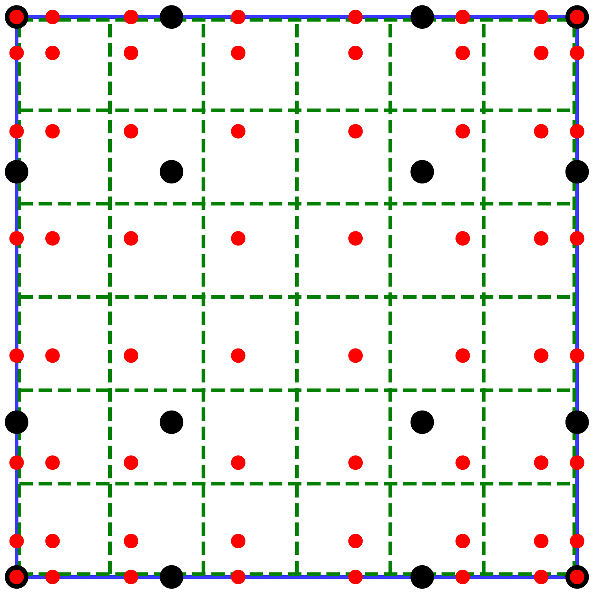
Figure 1 Diagram of subelement grids. One spectral element (blue solid line outlining the full square) with dynamics ($n_{\mathrm{p}}^{\mathrm{v}}=\mathrm{4}$, black large circles), tracer ($n_{\mathrm{p}}^{\mathrm{t}}=\mathrm{8}$, small red circles), and physics (n_f=6, green dashed lines) subelement grids.

In the horizontal direction, each quadrilateral element has an n_p×n_p subgrid. HOMME uses the Gauss–Legendre–Lobatto (GLL) spectral element polynomial basis and nodes. The two-dimensional (2D) basis functions are tensor products of one-dimensional (1D) GLL basis functions. n_p is the number of subgrid nodes in a 1D basis function; the degree of the polynomial is n_p−1. Figure 1 shows one spectral element outlined in blue. The large black dots are the 4×4 tensor-product grid of GLL nodes with n_p=4. The Courant–Friedrichs–Lewy (CFL) condition for the advection operator in spectral element fluid dynamics scales inversely with the minimum distance between GLL nodes. In turn, this minimum distance scales roughly quadratically in n_p. For example, nodes for n_p=6, 8, and 12 have minimum distances respectively 2.4, 4.3, and 10.0 times smaller than nodes for n_p=4. Thus, developers of a dynamics solver choose a value for n_p that is large enough to provide good accuracy and wave representation but small enough to permit a large time step, i.e., one determined by accuracy rather than stability considerations. EAM always sets $n_{\mathrm{p}}^{\mathrm{v}}=\mathrm{4}$, where we use v to refer specifically to the dynamics solver's value of n_p. We refer to the spectral element grid, including the spectral element nodes, as the dynamics grid, and the element grid excluding subgrid nodes as the element grid.

For efficiency, the EAM version 2 physics and chemistry parameterizations run on a different grid than the dynamics; we call this grid the physics grid. To couple efficiently to the dynamics grid, the physics grid has the same element grid as the dynamics grid but its own subelement grid (Herrington et al., 2019; Hannah et al., 2021). The physics grid divides each horizontal quadrilateral element into a regular n_f×n_f subgrid of finite-volume quadrilateral subcells. In Fig. 1, the dashed green lines outline the 6×6 physics subgrid, with n_f=6. EAM version 2 uses n_f=2. Compared with EAM version 1, in which the physics and dynamics grids were the same, EAM version 2 has $\mathrm{4}/\mathrm{9}$ as many physics grid points, speeding up the parameterizations part of the model by up to 2.25 times with a small cost for remapping between dynamics and physics grids. The shared element grid and the element-local remap operators minimize interprocess communication costs.

1.3 Overview of the Islet method

While our tracer transport method is based on spectral elements and, like the physics grid, uses the same element grid as the dynamics grid, it is not restricted by the CFL condition. This important fact motivates making $n_{\mathrm{p}}^{\mathrm{t}}$, where we use t to refer specifically to the transport solver's value of n_p, a parameter of the tracer transport module and independent of $n_{\mathrm{p}}^{\mathrm{v}}$, to trade between computational speed (maximum at $n_{\mathrm{p}}^{\mathrm{t}}=n_{\mathrm{p}}^{\mathrm{v}}$) and higher accuracy (increasing with $n_{\mathrm{p}}^{\mathrm{t}}$). In Fig. 1, the small red circles are GLL nodes for $n_{\mathrm{p}}^{\mathrm{t}}=\mathrm{8}$. We refer to this approach as tracer transport p-refinement. In the finite element method, p-refinement means increasing the basis polynomial degree. In the Islet method, we increase $n_{\mathrm{p}}^{\mathrm{t}}$ relative to $n_{\mathrm{p}}^{\mathrm{v}}$ to represent the mixing ratio fields at higher resolution.

In summary, we use one element grid, three subelement grids, and three corresponding parameters: the dynamics grid, $n_{\mathrm{p}}^{\mathrm{v}}$; the physics grid, n_f; and the tracer transport grid, $n_{\mathrm{p}}^{\mathrm{t}}$. For efficiency, EAM version 2 already uses two grids, one with $n_{\mathrm{p}}^{\mathrm{t}}=n_{\mathrm{p}}^{\mathrm{v}}=\mathrm{4}$ and the other with n_f=2. This article considers the case $n_{\mathrm{p}}^{\mathrm{t}}>n_{\mathrm{p}}^{\mathrm{v}}$. Figure 1 shows the three subgrids for one spectral element.

The tracer transport solver couples to the dynamics solver through the flow velocity u, the air density ρ, and possibly a small subset of tracers such as specific humidity. It couples to the parameterizations through the tracers. Coupling requires remapping a field between grids. It is natural to give responsibility for these remap procedures to the tracer transport solver module as the remap operators share many of the same requirements and computations as the transport solver. As in the case of remapping quantities between the physics grid and the dynamics grid in EAM version 2, the shared element grid and element-local remap procedures minimize communication when remapping among the three grids. For brevity, we refer to this overall spectral element, three-grid scheme as the Islet method.

1.4 Outline

The rest of this article is structured as follows. The Islet method depends on a number of lower-level algorithms. Section 2 and Appendix A describe these; mathematical details can be skipped on a first reading. Section 3 describes each step of the Islet method over the course of one time step. Descriptions are compact, relying on the details in Sect. 2. Section 4 describes and presents the results of a number of verification problems. Finally, Sect. 5 concludes.

2 Overview of algorithms

This section describes the details of low-level algorithms on which the Islet method depends, associated concepts, and related work for context. Our objective is to isolate the notation for and details of these low-level algorithms to this section, then focus on the higher-level details of the Islet method in Sect. 3 without lower-level clutter. Section 2.1 discusses semi-Lagrangian transport, the finite-element interpolation semi-Lagrangian method in particular, and the bases that the Islet method uses. Section 2.2 describes our approach to solving the property preservation problem. Section 2.3 describes algorithms to remap data between grids. Section 2.4 describes the spectral element direct stiffness summation operator.

2.1 Semi-Lagrangian transport

The Islet method uses semi-Lagrangian (SL) transport. In an SL method, following Eqs. (5) and (6), each Eulerian arrival grid point at time t₁ is advected backward or forward in time to its generally off-grid departure point at time t₀. The resulting Lagrangian departure grid then samples the field at time t₀ and, by some means, uses these data to construct the advected field at time t₁.

In the problem of tracer transport, for which the flow velocity u is provided, SL methods can take much longer time steps than Eulerian methods. Data dependencies are local to a small domain of dependence; thus, unlike an implicit method, SL tracer transport does not require the solution of a global linear equation. This long time step requires many fewer interprocess communication rounds and sometimes fewer floating point operations per unit of simulation time than Eulerian methods, making SL methods substantially more efficient than Eulerian methods for tracer transport.

Transport methods often are the composition of a number of operators. Two key operators are the linear advection operator and the nonlinear property preservation operator; we describe ours in Sect. 2.1.4 and 2.2, respectively.

2.1.1 Types of SL methods

For a broad survey of atmosphere tracer transport methods, including a large number of Lagrangian and semi-Lagrangian methods, we refer the reader to Lauritzen et al. (2014, Sect. 2). In addition, Giraldo et al. (2003), Natarajan and Jacobs (2020), and Bradley et al. (2019) review types of SL methods. This article focuses on remap-form interpolation methods.

A method in remap form directly remaps the tracer field on the Eulerian grid at the previous time step to the Lagrangian grid, in contrast to flux-form methods that integrate over swept regions (Lauritzen et al., 2010; Lee et al., 2016) or characteristic curves (Erath and Nair, 2014). The computational and communication costs of a remap-form method are very nearly independent of time step whereas a flux-form method's cost grows roughly linearly with the time step.

An interpolation SL (ISL) method directly discretizes the tracer transport equation, Eq. (5): $q({\mathit{x}}_i,t_{\mathrm{1}})=q({\overline{\mathit{x}}}_i,t_{\mathrm{0}})$, where x_i is an Eulerian arrival grid point and ${\overline{\mathit{x}}}_i$ is its departure, generally off-grid, point at t₀<t₁. q has exact values only at grid points x_i; thus, evaluating $q({\overline{\mathit{x}}}_i,t_{\mathrm{0}})$ requires interpolation.

Interpolation is in contrast to exactly cell-integrated methods, which accurately integrate the basis of a target (e.g., Lagrangian) element against those of the source; see, e.g., Bosler et al. (2019). (In some cases, an inaccurate cell-integrated method can be interpreted as an interpolation method; see Appendix B for an example.) Exactly cell-integrated methods have substantially greater cost than interpolation methods for three reasons.

First, to obtain smoothness in the integrand, integration is over facets computed by geometric intersection of a target element against source elements; intersection calculations are not needed in interpolation methods. Typically, to minimize computational geometry complexity, departure cell edges are approximated by great arcs rather than flow-distorted curves, limiting the method to second-order accuracy; however, Ullrich et al. (2013) describe a higher-order edge reconstruction that yields a third-order accurate advection method. In contrast, achieving arbitrarily high order in an ISL method's linear advection operator does not entail any additional complexity.

Second, accurate integration has a larger computational cost because it requires sphere-to-reference point calculation and interpolant evaluations at many quadrature points.

Third, an exactly cell-integrated method requires a larger communication volume because all data from a source element are used to integrate against each target basis function.

In trade for these additional costs, exactly cell-integrated methods are locally mass conserving, and the fact that they are L² projections can be used to prove stability. Local mass conservation means that one can identify numerical, possibly Lagrangian, fluid parcels on the grid that have constant tracer mass. Local is in contrast to global mass conservation; the latter means that the mass of the tracer fluid is conserved over the whole domain but not necessarily in any identifiable parcels smaller than the domain. Although an exactly cell-integrated method is locally mass conserving, coupling it to a dynamics solver still generally requires additional measures to obtain mass-tracer consistency.

2.1.2 Spectral element ISL transport

Our objective in this work is to use the design freedom provided by giving up local, but not global, mass conservation to maximize computational efficiency. We develop an ISL method that uses the Islet bases, summarized in Appendix A and derived in Bradley et al. (2021, Sects. 2 and 3) and a forthcoming article based on that material, to satisfy a necessary condition for stability.

Figure 2 Diagram of the linear advection operation in a finite-element interpolation semi-Lagrangian time step. (a) Six spectral elements (blue solid lines) with an $n_{\mathrm{p}}^{\mathrm{t}}=\mathrm{6}$ tracer grid (red small circles). The black large circles in the upper-left element show the $n_{\mathrm{p}}^{\mathrm{v}}=\mathrm{4}$ dynamics grid. The upper-left Eulerian arrival element is advected backward in time to the right and down, resulting in the Lagrangian departure element (blue dashed outline, open circle dynamics grid points, green tracer grid points). The domain of dependence of each green starred tracer grid point is the bottom right Eulerian element, with interpolation grid points (red small circles) associated with this domain of dependence outlined in black. (b) The six 1D $n_{\mathrm{p}}^{\mathrm{t}}=\mathrm{6}$ element basis functions, a different color for each, for the natural GLL (dashed curves) and Islet GLL (solid curves) bases. In the bottom right Eulerian element, a set of 1D basis functions is conceptually associated with each of the red horizontal and green vertical rectangles outlining an element side, and a 2D basis function over the element is a tensor product of one 1D basis function from each set.

Figure 2a illustrates the linear advection step in the Islet method. First, the upper-left element is advected backward in time from time t₁ to time t₀, using velocity data on the $n_{\mathrm{p}}^{\mathrm{v}}=\mathrm{4}$ dynamics grid to advect each dynamics grid point. Second, the $n_{\mathrm{p}}^{\mathrm{v}}=\mathrm{4}$ isoparametric map interpolates the locations of the Lagrangian $n_{\mathrm{p}}^{\mathrm{t}}=\mathrm{6}$ tracer grid points from the Lagrangian $n_{\mathrm{p}}^{\mathrm{v}}=\mathrm{4}$ dynamics grid points. Third, the tracer data at time t₀ in the bottom-right Eulerian element are used to interpolate the tracer mixing ratio at t₀ to each green starred Lagrangian point. Interpolation uses the 2D tensor-product $n_{\mathrm{p}}^{\mathrm{t}}=\mathrm{6}$ nodal basis. Fourth, these values are then the values in the upper-left Eulerian element at time t₁.

Figure 2b shows two bases, the GLL basis, called the natural basis when a distinguishing name is needed, and the Islet GLL basis. The ISL method using the natural GLL basis is unstable for the test problem of uniform flow on a uniform grid, but the ISL method using the Islet GLL basis is stable for this problem (Bradley et al., 2021). In this article, all of the algorithms accommodate either basis type, and we use the Islet GLL bases to obtain stability; see Appendix A for details.

Each basis is a nodal basis: a basis function has value 1 at one node and 0 at every other node. Thus, each basis function is associated with a node. For example, in Fig. 2b, the blue basis function is associated with the third node of six. The basis is symmetric; basis function $k\in \mathit{\{}\mathrm{0},\mathrm{\dots },n_{\mathrm{p}}-\mathrm{1}\mathit{\}}$ is the mirror image of basis function $n_{\mathrm{p}}-k-\mathrm{1}$. Thus, the blue and cyan functions are mirror images around reference coordinate 0.

There are two conventional ways to enumerate finite element nodal degrees of freedom and basis functions, where for a scalar field, one degree of freedom is associated with each basis function. First, in this article, by a basis we always mean an element basis unless stated otherwise. A basis function in an element basis set has non-zero values only within an element. As a result, nodes in the interior of an element have single-valued field values while nodes at an element boundary may have multi-valued field values.

Second, the viewpoint of global continuous degrees of freedom and global basis functions always assigns only one degree of freedom of the field to each grid point. The basis function associated with a grid point in the interior of an element is the same as in the element basis. A grid point on the element boundary has a basis function that spans all the elements that share that grid point. This global basis function is the sum of the element basis functions associated with that grid point.

In the case of continuous finite element methods, the two viewpoints are equivalent, and convenience determines which viewpoint is adopted. In the case of a discontinuous finite element method, only the element viewpoint is possible.

The Islet method accommodates both continuous and discontinuous variants; in this article, we present only the continuous variant. We always take the element viewpoint, regardless of the continuity of a field. Thus, for a scalar field, there is one degree of freedom associated with each grid point in an element and, thus, n degrees of freedom at a grid point shared by n elements. Index i is associated with grid point location x_i. Again, to be clear, for a grid point at an element edge, multiple index values are associated with the same location x. Some steps in the Islet method introduce discontinuities in the field across elements. Section 2.4 describes the operator that restores continuity to a discontinuous field.

2.1.3 Definitions and notation

The tracer mixing ratio degrees of freedom are written q_i and the air density, ρ_i. The vector of all scalar values is bold-faced, e.g., q. A subset of these, with the index set given by ℰ, is written q(ℰ). When needed, a superscript letter indicates on which grid the field is approximated: t, tracer; v, dynamics; and f, physics.

Arithmetic between vectors applies entry-wise. For two vectors, x and y, we write x⊙y for element-wise multiplication and x⊘y for element-wise division.

We need to define a map between a reference element with coordinates $\mathit{r}\in [-\mathrm{1},\mathrm{1}{]}^{\mathrm{2}}$ and element e on the manifold with coordinates x, e.g., the sphere. Let this map be x=m_e(r) and its inverse be $\mathit{r}=m_e^{-\mathrm{1}}\left(\mathit{x}\right)$. Additionally, let e=E(x) return the element index for the element that contains e. In this work, if x is on the boundary of multiple elements, E(x) can be any of the corresponding element indices without affecting the solution.

Similarly, we need to map between (element-)local and global indices. Local indices are in the set $\mathit{\{}\mathrm{0},\mathrm{\dots },(n_{\mathrm{p}}^g{)}^{\mathrm{2}}-\mathrm{1}\mathit{\}}$, where $g\in \mathit{\{}\mathrm{v},\mathrm{t}\mathit{\}}$. Global index i is in element $\mathrm{elm}(i;g)\equiv \lfloor i/(n_{\mathrm{p}}^g{)}^{\mathrm{2}}\rfloor$. The corresponding local index is $\mathrm{lcl}(i;g)\equiv i\mathrm{mod}(n_{\mathrm{p}}^g{)}^{\mathrm{2}}$. Given the local index j and element index e, the global index is $\mathrm{glb}(j;g)\equiv (n_{\mathrm{p}}^g{)}^{\mathrm{2}}e+j$. Let ℰ(e;g) be the set of global indices for the grid points in element e. We omit g when it is not necessary to specify a grid. For convenience, let q_e≡q(ℰ(e)).

Element basis functions and reference-coordinate nodes are indexed locally. Thus, global grid point i corresponds to the 2D tensor-product element basis function ϕ_lcl(i;g) and reference-coordinate node r_lcl(i;g).

Occasionally, we write the tensor product in the 2D basis explicitly. Let a 1D element basis function set be ψ_j, $j\in \mathrm{0},\mathrm{\dots },n_{\mathrm{p}}-\mathrm{1}$. Let $\mathit{r}\equiv (r_{\mathrm{1}},r_{\mathrm{2}})$. Then, ${\mathit{\varphi }}_i\left(\mathit{r}\right)\equiv {\mathit{\psi }}_{\lfloor i/n_{\mathrm{p}}\rfloor }\left(r_{\mathrm{1}}\right){\mathit{\psi }}_{i\mathrm{mod}{n}_{\mathrm{p}}}\left(r_{\mathrm{2}}\right)$. Figure 2b shows the $n_{\mathrm{p}}^{\mathrm{t}}=\mathrm{6}$ basis functions ψ_j.

The function $\mathrm{normalize}\left(\mathit{x}\right)\equiv \mathit{x}/\Vert \mathit{x}{\Vert }_{\mathrm{2}}$.

Finally, we write the particular map x=m_e(r) we use. The map uses just the corner nodes of an element; it is the isoparametric map for a bilinear basis. In element e, let corner_e(j;v) be the global index of corner j of the element, here referenced to the dynamics grid for concreteness. Let ${\mathit{\varphi }}_j^{\mathrm{bilin}}\left(\mathit{r}\right)$ be the bilinear basis functions, i.e., the GLL basis with n_p=2. Then,

$$\begin{array}{}\text{(7)}& \mathit{x}\left(\mathit{r}\right)=\mathrm{normalize}\left(\sum _{j=\mathrm{0}}^{\mathrm{3}}{\mathit{x}}_{\mathrm{corner}(j;\mathrm{v})}^{\mathrm{v}}{\mathit{\varphi }}_j^{\mathrm{bilin}}\left(\mathit{r}\right)\right).\end{array}$$

This is the map described in Guba et al. (2014, Appendix A).

2.1.4 The linear advection operator

Now we write the steps illustrated in Fig. 2. First, each grid point ${\mathit{x}}_i^{\mathrm{v}}$ is advected from time t₁ to time t₀ to give

$$\begin{array}{}\text{(8)}& {\overline{\mathit{x}}}_i^{\mathrm{v}}\equiv \mathit{X}(t_{\mathrm{0}};{\mathit{x}}_i^{\mathrm{v}},t_{\mathrm{1}}).\end{array}$$

In this article, we assume this step is performed nearly exactly, i.e., with numerical error substantially smaller than any other source of error because this article focuses on the spatial part of the advection discretization. Second, the tracer grid points are computed from the dynamics grid points using the $n_{\mathrm{p}}^{\mathrm{v}}$-basis isoparametric map followed by normalization:

$$\begin{array}{}\text{(9)}& {\overline{\mathit{x}}}_i^{\mathrm{t}}\equiv \mathrm{normalize}\left(\sum _{j\in {\mathcal{E}}^{\mathrm{v}}\left(\mathrm{elm}\right(i;\mathrm{t}\left)\right)}{\overline{\mathit{x}}}_j^{\mathrm{v}}{\mathit{\varphi }}_{\mathrm{lcl}(j;\mathrm{v})}^{\mathrm{v}}\left({\mathit{r}}_{\mathrm{lcl}(i;\mathrm{t})}^{\mathrm{t}}\right)\right).\end{array}$$

Third, an interpolated value from time t₀ is assigned to each advected tracer grid point:

$$\begin{array}{}\text{(10)}& {\displaystyle }e& {\displaystyle }\equiv E\left({\overline{\mathit{x}}}_i^{\mathrm{t}}\right)\text{(11)}& {\displaystyle }{q}_i^{\mathrm{t}}\left(t_{\mathrm{1}}\right)& {\displaystyle }=\sum _{j\in {\mathcal{E}}^{\mathrm{t}}\left(e\right)}{q}_j^{\mathrm{t}}\left(t_{\mathrm{0}}\right){\mathit{\varphi }}_{\mathrm{lcl}(j;\mathrm{t})}^{\mathrm{t}}\left(m_e^{-\mathrm{1}}\right({\overline{\mathit{x}}}_i^{\mathrm{t}}\left)\right).\end{array}$$

2.2 Property preservation

Shape preservation and mass conservation on their own are not necessarily difficult to achieve. Rather, the hard problem in the development of an efficient transport method is the consistent coupling of the transport scheme to the dynamical core, or mass-tracer consistency. Mass-tracer consistency means that the transport solver and dynamics solver agree exactly on the air density field. Achieving both mass-tracer consistency and a long transport time step requires redistributing tracer mass.

It is possible to couple a tracer transport method to a dynamical core consistently and preserve properties using only local operations. Lauritzen et al. (2017) describe the coupling of a finite-volume, cell-integrated SL method to the HOMME spectral element dynamical core using Lagrangian grid adjustments, where each adjustment is a function of only data in the adjusted entity's local neighborhood. However, in their method, the time step is limited to a Courant number of at most 1, limiting efficiency.

Our approach to consistent coupling is to use what is sometimes called a global fixer, although, often, this term applies to only the problem of global mass conservation. In Bradley et al. (2019), we describe several classes of methods that we call Communication-Efficient Density Reconstructors (CEDR). Each CEDR can solve a variety of property preservation problems, including shape preservation and global mass conservation. Each CEDR provides a tight and practically meaningful bound on mass redistribution. A solution is assured if the input data meet necessary and sufficient conditions. Depending on the algorithm, a CEDR uses either one or two global reductions or reduction-like communication rounds. See Bradley et al. (2019, Sect. 1.2) for a discussion of how CEDRs relate to previous global fixers, in particular, with respect to solution guarantees and number of communication rounds.

Because we use a CEDR for consistent coupling, we are then free to exploit it in other parts of our transport method to maximize efficiency. For example, we can use an interpolation SL method, which is not mass conserving, because the mass will be corrected at the end of each time step.

Exact shape preservation uses mixing ratio bounds computed from each arrival grid point's domain of dependence and does not permit any violation of a domain's nodal extrema. As a result, exact shape preservation clips smooth extrema, limiting the overall transport method to an order of accuracy generally not more than a little above two. Nonetheless, higher-order linear advection is still useful because it increases the absolute accuracy of the overall method even if not its order of accuracy, as examples in Sect. 4 will demonstrate.

2.2.1  ClipAndAssuredSum

In this article, we use the simplest CEDR: ClipAndAssuredSum, subsequently CAAS, algorithm 3.1 in Bradley et al. (2019).

To explain CAAS, we need to define the weight associated with a grid point since weights are needed to define the mass. Conceptually, a weight is an integral over the element of the product of the grid point's basis function and the Jacobian determinant of x=m(r):

$$\begin{array}{}\text{(12)}& {\overline{\mathit{\theta }}}_i\equiv \underset{-\mathrm{1}}{\overset{\mathrm{1}}{\int }}\underset{-\mathrm{1}}{\overset{\mathrm{1}}{\int }}{\mathit{\varphi }}_{\mathrm{lcl}\left(i\right)}\left(\mathit{r}\right)\left|{\displaystyle \frac{\partial m_{\mathrm{elm}\left(i\right)}\left(\mathit{r}\right)}{\partial \mathit{r}}}\right|\mathrm{d}\mathit{r}.\end{array}$$

Details of the discretization modify this value. Our manifold is the sphere, and we use HOMME's definition of a weight. HOMME discretizes the weight integral using the n_p-basis GLL quadrature. Let

$$v_i\equiv \underset{-\mathrm{1}}{\overset{\mathrm{1}}{\int }}{\mathit{\psi }}_i\left(r\right)\mathrm{d}r.$$

Because ϕ_lcl(i)(r_lcl(j))=1 when j=i and is 0 for every other value of j, GLL quadrature applied to Eq. (12) gives

$$\begin{array}{ll}{\displaystyle }{\mathit{\theta }}_i& {\displaystyle }\equiv \sum _{j\in \mathcal{E}\left(\mathrm{elm}\right(i\left)\right)}\left[{\mathit{\varphi }}_{\mathrm{lcl}\left(i\right)}\left({\mathit{r}}_{\mathrm{lcl}\left(j\right)}\right)\left|{\displaystyle \frac{\partial m_{\mathrm{elm}\left(i\right)}\left({\mathit{r}}_{\mathrm{lcl}\left(j\right)}\right)}{\partial \mathit{r}}}\right|\right]\times \\ {\displaystyle }& {\displaystyle }{v}_{\lfloor \mathrm{lcl}\left(j\right)/n_{\mathrm{p}}\rfloor }{v}_{\mathrm{lcl}\left(j\right)\mathrm{mod}{n}_{\mathrm{p}}}\\ {\displaystyle }& {\displaystyle }=\left|{\displaystyle \frac{\partial m_{\mathrm{elm}\left(i\right)}\left({\mathit{r}}_{\mathrm{lcl}\left(i\right)}\right)}{\partial \mathit{r}}}\right|v_{\lfloor \mathrm{lcl}\left(i\right)/n_{\mathrm{p}}\rfloor }{v}_{\mathrm{lcl}\left(i\right)\mathrm{mod}{n}_{\mathrm{p}}}\\ {\displaystyle }& {\displaystyle }\equiv J_i{w}_i.\end{array}$$

In the final line, we define

$$\begin{array}{}\text{(13)}& J_i\equiv \left|{\displaystyle \frac{\partial m_{\mathrm{elm}\left(i\right)}\left({\mathit{r}}_{\mathrm{lcl}\left(i\right)}\right)}{\partial \mathit{r}}}\right|\end{array}$$

and w_i as the product of the two 1D basis function integrals. In practice, HOMME modifies each node's Jacobian determinant J_i by multiplying it by a constant very close to 1 such that the global sum ${\sum }_i{J}_i{w}_i=\mathrm{4}\mathit{\pi }$; that is, the sum of all the products of w_i and adjusted J_i gives exactly the area of the unit sphere. This is an optional and minor implementation detail, and we neglect this scaling factor subsequently. Note that, in general, J is discontinuous across elements.

Now we describe CAAS independent of two sets of details: first, the means by which time-t₁ data are obtained and, second, the index set ℰ over which CAAS is applied. Later, we will specify these details for each application of CAAS. At time t₁ and grid point i, we are given air density ρ_i, preliminary tracer mixing ratio ${\overline{q}}_i$, and weight θ_i. In addition, we are given a target total mass b over all i∈ℰ. Finally, we have lower and upper bounds, $q_i^{min}$ and $q_i^{max}$, on the target q_i. These are the inputs to CAAS. The output is a set of modified values q(ℰ) that solve the 1-norm minimization problem

$$\begin{array}{ll}{\displaystyle }min& {\displaystyle }\sum _{i\in \mathcal{E}}|q_i-{\overline{q}}_i|\\ {\displaystyle }\text{subject to}& {\displaystyle }\sum _{i\in \mathcal{E}}{\mathit{\theta }}_i{\mathit{\rho }}_i{q}_i=b& {\displaystyle }\text{(mass conservation)}\\ {\displaystyle }& {\displaystyle }{q}_i^{min}\le q_i\le q_i^{max}\mathrm{for}i\in \mathcal{E}& {\displaystyle }\text{(shape preservation)}.\end{array}$$

This problem has a solution, i.e., the constraint set is non-empty, if and only if

$$\begin{array}{}\text{(14)}& \sum _{i\in \mathcal{E}}{\mathit{\theta }}_i{\mathit{\rho }}_i{q}_i^{min}\le b\le \sum _{i\in \mathcal{E}}{\mathit{\theta }}_i{\mathit{\rho }}_i{q}_i^{max}.\end{array}$$

For details, see Bradley et al. (2019, Sect. 2).

When there is a solution, there are usually an infinite number, and CAAS efficiently finds one as follows. First, clip the mixing ratios for i∈ℰ:

$${\widehat{q}}_i\equiv min(q_i^{max},max(q_i^{min},{\overline{q}}_i\left)\right).$$

Let the preliminary mass be

$$\widehat{m}\equiv \sum _{i\in \mathcal{E}}{\mathit{\theta }}_i{\mathit{\rho }}_i{\widehat{q}}_i.$$

If $\widehat{m}=b$, then set $q_i={\widehat{q}}_i$ for i∈ℰ and terminate. Otherwise, suppose $\widehat{m}<b$. Second, compute the capacity:

$$c\equiv \sum _{i\in \mathcal{E}}{\mathit{\theta }}_i{\mathit{\rho }}_i(q_i^{max}-{\widehat{q}}_i).$$

Third, compute the final values for i∈ℰ:

$$q_i={\widehat{q}}_i+(b-\widehat{m}){\displaystyle \frac{q_i^{max}-{\widehat{q}}_i}{c}}.$$

As a check, note that

$$\begin{array}{ll}{\displaystyle }\sum _{i\in \mathcal{E}}{\mathit{\theta }}_i{\mathit{\rho }}_i{q}_i& {\displaystyle }=\sum _{i\in \mathcal{E}}{\mathit{\theta }}_i{\mathit{\rho }}_i{\widehat{q}}_i+(b-\widehat{m}){\displaystyle \frac{{\sum }_{i\in \mathcal{E}}{\mathit{\theta }}_i{\mathit{\rho }}_i(q_i^{max}-{\widehat{q}}_i)}{c}}\\ {\displaystyle }& {\displaystyle }=\widehat{m}+(b-\widehat{m}){\displaystyle \frac{c}{c}}\\ {\displaystyle }& {\displaystyle }=b.\end{array}$$

If $b-\widehat{m}\le c$, then $q_i\le q_i^{max}$ for i∈ℰ; these conditions hold if and only if Eq. (14) does. The case $\widehat{m}>b$ is similar. Let

$$\mathit{q}\left(\mathcal{E}\right)=\mathrm{CAAS}(\mathcal{E},\mathit{\rho },\mathit{\theta },b,{\mathit{q}}^{min},{\mathit{q}}^{max},\overline{\mathit{q}})$$

carry out these steps.

CAAS is a CEDR because the global version, i.e., the problem in which ℰ is over all grid points, can be implemented using a single global reduction. For details, see Bradley et al. (2019, Sect. 6).

2.2.2 Infeasible problems

In some situations, the constraint set is empty. There is a sequence of up to two relaxations to the constraints to produce a non-empty constraint set. Algorithm 3.4 in Bradley et al. (2019), ReconstructSafely, which wraps a lower-level algorithm like CAAS, formalizes this sequence. Suppose the original constraint set is empty and $\widehat{m}<b$. ReconstructSafely first tries to compute a one-norm-minimal relaxation to q^max, such that the maximum value ${max}_{i\in \mathcal{E}}{q}_i^{max}$ is not exceeded:

$$\begin{array}{ll}{\displaystyle }\mathit{q}\left(\mathcal{E}\right)=& {\displaystyle }{\mathit{q}}^{max}\left(\mathcal{E}\right)+\\ {\displaystyle }& {\displaystyle }\mathrm{CAAS}(\mathcal{E},\mathit{\rho },\mathit{\theta },b-\sum _{i\in \mathcal{E}}{\mathit{\theta }}_i{\mathit{\rho }}_i{q}_i^{max},\mathbf{0},\\ {\displaystyle }& {\displaystyle }\underset{i\in \mathcal{E}}{max}{q}_i^{max}-\mathit{q},{\mathit{q}}^{max}).\end{array}$$

This relaxed problem provides mass-tracer consistency and mass conservation but does not solve the exact shape preservation problem. If this relaxation has an empty constraint set, then ReconstructSafely returns q(ℰ) with uniform values that satisfy the mass conservation constraint.

2.2.3 Local and global problems

We use CAAS to solve problems at two levels: first, within each element separately and, second, over the whole grid. In addition, at the global level, there are two natural choices for scalar values in the vectors passed to CAAS: grid point values and integrals over elements. In practice, some local problems may not have assuredly non-empty constraint sets, but the global problem always has a non-empty constraint set.

In the first approach to the global problem, which we refer to as CAAS–point, the inputs to CAAS are simply the grid point values. Global and local applications of CAAS are then identical except for the index set ℰ.

In the alternative approach, which we refer to as CAAS–CAAS, the global problem is solved over element-level scalar values, and then a second step applies CAAS separately to each element. The global step's task is to provide each element with a sufficient mass adjustment so that each element's local CAAS step has a non-empty constraint set. The global problem's inputs are formulated as follows. Weight e is element e's area: $A_e\equiv {\sum }_{i\in \mathcal{E}\left(e\right)}{w}_i{J}_i$. Air density ρ_e is the element's average density. Let the element's mass be $m_e\equiv {\sum }_{i\in \mathcal{E}\left(e\right)}{w}_i{J}_i{\mathit{\rho }}_i$. Then, ${\mathit{\rho }}_e=m_e/A_e$. The minimum mixing ratio is the minimum tracer mass over the element divided by the total mass: $q_e^{min}\equiv {\sum }_{i\in \mathcal{E}\left(e\right)}{w}_i{J}_i{\mathit{\rho }}_i{q}_i^{min}/m_e$, and similarly for $q_e^{max}$. Finally, the initial value ${\overline{q}}_e$ is ${\overline{q}}_e\equiv {\sum }_{i\in \mathcal{E}\left(e\right)}{w}_i{J}_i{\mathit{\rho }}_i{q}_i/m_e$. This global CAAS step returns element-level mass adjustments. The adjusted mass in an element is then b in the input to the local CAAS step.

2.2.4 Relaxed problems

In the Islet method, multiple local and one global property preservation problems are solved in each time step. Not every problem must enforce strict property preservation; strictness is required only in certain outputs, e.g., at the end of a time step. Relaxing the extremal bounds on the mixing ratio grid point values reduces the amount of mass redistribution. More subtly, solving relaxed element-local problems before solving the strict global problem increases intra-element and decreases inter-element mass redistribution, thus, increasing the locality of mass redistribution. Finally, problems such as the toy chemistry problem described in Sect. 4.3.2 that are sensitive to finite-precision round-off errors benefit from relaxed bounds because the perturbation to the mixing ratio is decreased. Thus, in some element-local CAAS applications in a time step, for each index i, we widen each pair of bounds by 1 % of $q_i^{max}-q_i^{min}$ in each direction. The global CAAS–point application uses strict bounds, assuring the tracer field is property-preserving at the end of a time step.

2.3 Grid remap

Remapping data among multiple component grids is common in many applications of partial differential equation (PDE)-based modeling because it is a direct means to permit each component to run in its most efficient configuration. For example, many whole-earth, fully coupled earth system models use different grids for ocean, land, and atmosphere components. Remapping among subcomponent grids is less common. Recent examples include separate physics parameterizations and dynamics grids in the atmosphere (Herrington et al., 2019; Hannah et al., 2021); adaptive mesh refinement (AMR) of a tracer (Chen et al., 2021; Semakin and Rastigejev, 2020); and local vertical refinement in physics parameterizations relative to the shared background vertical grid, the Framework for Improvement by Vertical Enhancement (FIVE) (Yamaguchi et al., 2017; Lee et al., 2020).

In the Islet method, grid remap operators transfer data among the dynamics, tracer, and physics grids. In all of these grid transfers, there is one key property: the linear remap operators use only element-local data. Thus, remap between grids is extremely efficient.

Remapping a field between a GLL grid, dynamics or tracer, and the physics grid is described in detail in Hannah et al. (2021, Sect. 2), and these details are not reproduced here. Remapping from the dynamics grid to the physics grid is simple: a physics grid subcell's value is assigned the average value of the density over the subcell. Remapping from the physics grid to the dynamics grid requires a high-order reconstruction of the data on the physics grid in addition to maintaining an element-local mass-conservation constraint, and most of the details in Hannah et al. (2021, Sect. 2) focus on this high-order reconstruction.

Remapping a field between the dynamics and tracer grids in either direction is simple; each grid hosts a field already in a high-order representation and, thus, no high-order reconstruction is needed. The first step is interpolation. Let ℐ^v→t interpolate a field in an element on the dynamics grid represented by the natural GLL $n_{\mathrm{p}}^{\mathrm{v}}$-basis to one on the tracer grid represented by the Islet $n_{\mathrm{p}}^{\mathrm{t}}$-basis, using the natural $n_{\mathrm{p}}^{\mathrm{v}}$-basis functions to interpolate. Let ℐ^t→v do the opposite using the Islet $n_{\mathrm{p}}^{\mathrm{t}}$-basis functions. We can write these linear operators explicitly using the notation introduced in Sect. 2.1.2. Let f be the grid-point values of a scalar field. Consider element e. Then, for local index $i\in \mathit{\{}\mathrm{0},\mathrm{\dots },(n_{\mathrm{p}}^{\mathrm{t}}{)}^{\mathrm{2}}-\mathrm{1}\mathit{\}}$,

$$({\mathit{f}}_e^{\mathrm{t}}{)}_i={\left({\mathcal{I}}^{\mathrm{v}\to \mathrm{t}}{\mathit{f}}_e^{\mathrm{v}}\right)}_i\equiv \sum _{j\in {\mathcal{E}}^{\mathrm{v}}\left(e\right)}{f}_j^{\mathrm{v}}{\mathit{\varphi }}_{\mathrm{lcl}(j;\mathrm{v})}^{\mathrm{v}}({\mathit{r}}_i^{\mathrm{t}}),$$

where we have used the notation f_e≡f(ℰ(e)). ℐ^t→v is written the same way but with t and v switched.

The interpolation of a field f from the dynamics grid to the tracer grid has the useful property that it is conservative within each element e despite not being in all cases an L² projection. Consider ${\mathit{f}}_e^{\mathrm{t}}={\mathcal{I}}^{\mathrm{v}\to \mathrm{t}}{\mathit{f}}_e^{\mathrm{v}}$. Then,

$$\begin{array}{}\text{(15)}& \sum _{i\in {\mathcal{E}}^{\mathrm{t}}\left(e\right)}{w}_i^{\mathrm{t}}{f}_i^{\mathrm{t}}=\sum _{i\in {\mathcal{E}}^{\mathrm{v}}\left(e\right)}{w}_i^{\mathrm{v}}{f}_i^{\mathrm{v}}.\end{array}$$

See Appendix A2 for a proof of Eq. (15).

Remapping between grids requires, as a second step, applying CAAS for property preservation; thus, we need grid point weight data on each grid. We define J^t using Eq. (13). On the tracer grid, rather than use Eq. (13), we interpolate the Jacobian determinant values from the dynamics grid,

$$\begin{array}{}\text{(16)}& {\mathit{J}}_e^{\mathrm{t}}={\mathcal{I}}^{\mathrm{v}\to \mathrm{t}}{\mathit{J}}_e^{\mathrm{v}},\end{array}$$

for two reasons. First, this operation conserves the area of the element,

$$\sum _{j\in {\mathcal{E}}^{\mathrm{t}}\left(e\right)}{w}_i^{\mathrm{t}}{J}_i^{\mathrm{t}}=\sum _{j\in {\mathcal{E}}^{\mathrm{v}}\left(e\right)}{w}_i^{\mathrm{v}}{J}_i^{\mathrm{v}},$$

by Eq. (15). We describe the second reason when discussing ρ in Sect. 3.1. On the physics grid, we follow a similar procedure, explained in Hannah et al. (2021, Sect. 2.2.1), that is specialized to the finite-volume physics grid. Here again, the area of an element on the physics grid is the same as on the dynamics grid. Thus, all three subgrid definitions of the element area agree on element area values.

2.4 Direct stiffness summation

In a spectral element method, most operations are performed independently in each element, often leading to discontinuities in a field across element boundaries. The global direct stiffness summation (DSS) operator (Fischer and Patera, 1989; Dennis et al., 2012) restores continuity. At each grid point on an edge of an element, the multi-valued solution is restored to a single value by weighted summation of contributions from each element sharing the grid point. An element's weight at grid point i is the value w_iJ_i normalized by the sum of all contributing elements' values. We will need a generalization of this operator in which an extra factor σ_i is absorbed into the weight in the weighted sum. Let ${\mathit{\delta }}_{ij}^{\mathrm{grid}}$ be 1 if global indices i and j are associated with the same grid point and 0 otherwise. For global index i, the generalized DSS applied to a preliminary field $\overline{\mathit{y}}$ is written:

$$\begin{array}{}\text{(17)}& y_i=\mathrm{DSS}(\mathit{\theta },\mathit{\sigma },\overline{\mathit{y}},i)\equiv {\displaystyle \frac{{\sum }_e{\sum }_{j\in \mathcal{E}\left(e\right)}{\mathit{\delta }}_{ij}^{\mathrm{grid}}{\mathit{\theta }}_j{\mathit{\sigma }}_j{\overline{y}}_j}{{\sum }_e{\sum }_{j\in \mathcal{E}\left(e\right)}{\mathit{\delta }}_{ij}^{\mathrm{grid}}{\mathit{\theta }}_j{\mathit{\sigma }}_j}},\end{array}$$

where ∑_e is the sum over all elements. In our use of the generalized DSS, σ=ρ and $\overline{\mathit{y}}=\overline{\mathit{q}}$. In the standard DSS, σ is all one and $\overline{\mathit{y}}=\mathit{\rho }\odot \overline{\mathit{q}}$. These two use cases give the same value for q_i if ρ is continuous across elements. We use the generalized DSS when we want to make q continuous but leave ρ discontinuous and, in particular, unmodified from its original value.

3 The Islet method

Now that we have described the problem setting and the core algorithms we use, we describe each algorithm that runs in one time step of the Islet method, advancing the simulation from time step n to n+1.

As part of an earth system model, the advection equation Eq. (3) has a source term. f is a function of possibly all the variables in a simulation. The physics parameterizations compute f on the physics grid. In practice, there are multiple equations of the form Eq. (3) to solve, e.g., 40 in the E3SM version 2 water cycle simulations (Golaz et al., 2022); because they decouple during one transport time step, we can focus on just one in this section.

In summary, first, air density ρ and trajectory data are remapped from the dynamics grid to the tracer grid. Second, Δq≡fΔt is remapped from the physics grid to the tracer grid, where Δt is the physics parameterization time step. Either of f or Δq is sometimes called a tendency. Third, the remapped tracer tendencies are added to the tracer-grid tracers. Fourth, the tracers are advected on the tracer grid. Fifth, tracer states are remapped to the physics and, optionally, dynamics grids.

3.1 Algorithms

There are a number of algorithmic steps in a time step. To organize these algorithms, we name each algorithm using the format Step::algorithm-name and sometimes Step::algorithm-name::sub-algorithm-name.

Step::density-d2t. Interpolate $\mathit{J}\odot {\mathit{\rho }}^{n+\mathrm{1}}$ from the dynamics grid to the tracer grid. In each element e, compute

$$({\mathit{\rho }}_e^{\mathrm{t}}{)}^{n+\mathrm{1}}=({\mathcal{I}}^{\mathrm{v}\to \mathrm{t}}({\mathit{J}}_e^{\mathrm{v}}\odot ({\mathit{\rho }}_e^{\mathrm{v}}{)}^{n+\mathrm{1}}\left)\right)\oslash {\mathit{J}}_e^{\mathrm{t}}.$$

This grid transfer conserves ${\mathit{J}}_e\odot {\mathit{\rho }}_e^{n+\mathrm{1}}$ by Eq. (15). ${\mathit{J}}^{\mathrm{t}}\odot ({\mathit{\rho }}^{\mathrm{t}}{)}^{n+\mathrm{1}}$ is not continuous across element boundaries because J^t is not, but continuity is not needed. Equation (16) implies that if ρ_e is constant on the dynamics grid, then it is constant on the tracer grid too. Mapping a constant air density exactly is not necessary, but since it is possible, we do; this property is the second reason to define J^t according to Eq. (16).

Step::tendency-f2t. Map the tracer tendency Δqⁿ from the physics grid to the tracer grid. This step involves multiple sub-algorithms.

Step::tendency-f2t::bounds. In each element e, compute and store the minimum and maximum values of $({\mathit{q}}_e^{\mathrm{f}}{)}^n$, subsequently, extrema. Let an element's neighborhood contain itself and every other element that shares a vertex with it. Augment an element's extrema with the extrema over its neighborhood. Finally, augment element e's extrema again with the extremal values of the tracer-grid mixing ratio state $({\mathit{q}}_e^{\mathrm{t}}{)}^n$. This final extrema update assures that if $\mathrm{\Delta }({\mathit{q}}_e^{\mathrm{f}}{)}^n=\mathrm{0}$, then $({\overline{\mathit{q}}}_e^{\mathrm{t}}{)}^n$ is unmodified in Step::tendency-f2t::CAAS. These final extrema are the bounds used in subsequent property preservation corrections.

Step::tendency-f2t::linear-remap. In each element e, apply the linear, element-local, conservative, panel-reconstruction remap operator described in Hannah et al. (2021, Sect. 2.2.3) to map the tendency from the physics grid to the tracer grid. In the Islet method, but unlike in Hannah et al. (2021), the basis used in the mass matrix of the L² projection is the Islet basis. From the previous step's application of Step::density-d2t, we have ${\mathit{\rho }}_e^{\mathrm{t}}$. The operator uses this quantity and ${\mathit{\rho }}_e^{\mathrm{f}}\odot \mathrm{\Delta }({\mathit{q}}_e^{\mathrm{f}}{)}^n$ to compute ${\mathit{\rho }}_e^{\mathrm{t}}\odot \mathrm{\Delta }({\mathit{q}}_e^{\mathrm{t}}{)}^n$.

Step::tendency-f2t::CAAS. In each element e, apply CAAS, described in Sect. 2.2.1, to $({\overline{\mathit{q}}}_e^{\mathrm{t}}{)}^n\equiv ({\mathit{q}}_e^{\mathrm{t}}{)}^n+\mathrm{\Delta }({\mathit{q}}_e^{\mathrm{t}}{)}^n$, using the weight vector ${\mathit{\theta }}_e^{\mathrm{t}}\equiv {\mathit{w}}_e^{\mathrm{t}}\odot {\mathit{J}}_e^{\mathrm{t}}$ and air density $({\mathit{\rho }}_e^{\mathrm{t}}{)}^n$. Target mass b is set to the current total element mass because Step::tendency-f2t::linear-remap is conservative; thus, no adjustment to the total element mass is needed. The same upper and lower bounds apply to each GLL node in the element. In this step, the bounds that Step::tendency-f2t::bounds computed are relaxed in each direction by 1 % of the difference between upper and lower bounds, as discussed in Sect. 2.2.4. The exact bounds will be enforced in Step::CEDR::global. The constraint set of mass conservation and bounds nonviolation is non-empty because the constant mixing ratio is a solution, as explained in Hannah et al. (2021, Sect. 2.3).

Step::tendency-f2t::DSS. At this point, $({\overline{\mathit{q}}}^{\mathrm{t}}{)}^n$ is discontinuous across element boundaries. Neither order of accuracy nor property preservation requires continuity, but we find that continuity improves the solution quality. (ρ^t)ⁿ can remain discontinuous. Thus, we apply the generalized DSS, Eq. (17), to $({\overline{\mathit{q}}}^{\mathrm{t}}{)}^n$, using (ρ^t)ⁿ to obtain the continuous field $({\widehat{\mathit{q}}}^{\mathrm{t}}{)}^n$.

Step::advect-interp. Compute and apply the linear advection ISL operator described in Sect. 2.1.4. This step involves two substeps: computing the grid point trajectories and computing the interpolants.

Step::advect-interp::trajectory. Compute Eq. (8). The dynamics component supplies velocity data at the dynamics GLL grid points. Any of a number of algorithms can compute departure points at time n backward in time from dynamics-grid arrival GLL points at time n+1. The Islet method takes as input these departure points as 3D Cartesian departure points. Next, compute Eq. (9). In each element, the natural GLL interpolant ℐ^v→t is applied to each of the Cartesian components separately to provide departure points on the tracer grid. This procedure implies that adjacent elements compute identical departure points at shared boundaries. Finally, for simplicity in the subsequent sphere-to-reference map computations, the 3D Cartesian points are normalized to the sphere. For $n_{\mathrm{p}}^{\mathrm{v}}=\mathrm{4}$, the $n_{\mathrm{p}}^{\mathrm{t}}$-basis departure points are obtained at order of accuracy 4.

Step::advect-interp::mixing-ratio. Compute Eq. (10). Each departure tracer-grid GLL node is mapped to the containing element, subsequently the source element. Details of finding the source element depend on host-model implementation details and are omitted here; possibilities include octree search, O(1) arithmetic for quasiuniform cubed-sphere element grids having certain reference-to-sphere maps, and search within a predefined element neighborhood whose size is proportional to maximum wind speed times advection time step. Then, the corresponding reference coordinates within the source element are computed using Newton's method. Next, compute Eq. (11). The mixing ratio value is computed at the departure point using the Islet basis interpolant and the source element's $({\widehat{\mathit{q}}}^{\mathrm{t}}{)}^n$ values. In addition, the source element's stored extrema are associated to this point as bounds. Finally, the mixing ratio value and bounds are assigned to the target GLL node on the arrival tracer grid. Departure points and interpolant weights are calculated once and then are reused for each tracer.

Step::CEDR. Apply Communication-Efficient Density Reconstructors (CEDR) on the tracer grid, first to each element and then globally. In this work, we use CAAS, described in Sect. 2.2.1. Node weights are w^t⊙J^t.

Step::CEDR::local. First, apply the element-local CAAS algorithm. This step is not required but it reduces the amount of global mass redistribution in Step::CEDR::global, is computationally inexpensive, involves no interprocess communication, and, thus, is worth including. As in Step::tendency-f2t::CAAS, we relax bounds in each direction by 1 % of the difference between upper and lower bounds. Unlike in Step::tendency-f2t::CAAS, in this application of the element-local CAAS algorithm, any two target GLL nodes in an element may have different bounds; the bounds depend on the source element for the target GLL node, as detailed in Step::advect-interp::mixing-ratio. At this point, the global mass has not yet been corrected; thus, this local CAAS application's mass constraint is to maintain the element's current tracer mass. The constraint set is not assuredly non-empty. Thus, ReconstructSafely, described in Sect. 2.2.2, wraps the call to CAAS.

Step::CEDR::global. Apply CAAS–point, described in Sect. 2.2.3, on the global tracer grid. The exact rather than relaxed bounds are applied to each node. The inputs to CAAS–point are as follows: the air density (ρ^t)ⁿ⁺¹; the weights $\mathit{\theta }\equiv {\mathit{w}}^{\mathrm{t}}\odot {\mathit{J}}^{\mathrm{t}}$; $b={\sum }_i{w}_i^{\mathrm{t}}{J}_i^{\mathrm{t}}\left({\mathit{\rho }}_i^{\mathrm{t}}{)}^n\right({\widehat{\mathit{q}}}^{\mathrm{t}}{)}^n$, the global tracer mass after the tendency update; the mixing ratio bounds computed in Step::tendency-f2t::bounds; and the current mixing ratio values from Step::CEDR::local. Let the output values be (q^t)ⁿ⁺¹.

Continuity across element boundaries was restored to the mixing ratio field in Step::tendency-f2t::DSS. Subsequent steps maintain it in exact arithmetic. However, in finite precision, continuity in (q^t)ⁿ⁺¹ holds only to a little above machine precision and not exactly. This numerical discontinuity does not grow in time because in each time step, both Step::tendency-f2t::DSS and Step::advect-interp::mixing-ratio restore exact continuity in finite precision, although only one restoration per time step is necessary to prevent growth of the numerical discontinuity. No step of the overall algorithm is sensitive to this small and roughly temporally constant numerical discontinuity.

At this point, the time step is complete; the remaining computations remap the tracer grid data between grids.

Step::state-t2f. Remap the mixing ratio state to the physics grid. This is a purely element-local operation. First, the linear operator described in Hannah et al. (2021, Sect. 2.2.1) is applied to the tracer density. Second, the element-local CAAS algorithm is applied on the physics grid, with the extremal mixing ratio values in the element on the tracer grid as the bounds. For the same reason as in Step::tendency-f2t::CAAS, the constraint set is assuredly non-empty.

Step::state-t2v. The dynamics solver needs one or more mixing ratios on the dynamics grid, e.g., specific humidity. In addition, in our numerical results in Sect. 4, we compute all errors, except as indicated, on the dynamics grid, so we use this step to obtain those errors. First, in an element, ℐ^t→v interpolates the tracer-grid mixing ratio to the $n_{\mathrm{p}}^{\mathrm{v}}$-basis. Second, the element-local CAAS algorithm is applied on the dynamics grid to preserve shape and conserve mass; the details are as in Step::state-t2f but with GLL nodes instead of finite-volume subcells. The result is (q^v)ⁿ⁺¹. Third, the standard DSS is applied to $({\mathit{\rho }}^{\mathrm{v}}{)}^{n+\mathrm{1}}\odot ({\mathit{q}}^{\mathrm{v}}{)}^{n+\mathrm{1}}$, where (ρ^v)ⁿ⁺¹ is the continuous air density from the dynamical core to obtain continuous tracer density and mixing ratio fields.

Step::state-v2t. In verification problems in Sect. 4, we need to remap a mixing ratio initial condition from the dynamics grid to the tracer grid. The algorithm is the same as Step::state-t2v except that the DSS follows the procedure in Step::tendency-f2t::DSS because the air density on the tracer grid is and remains discontinuous at element boundaries.

If $n_{\mathrm{p}}^{\mathrm{t}}=n_{\mathrm{p}}^{\mathrm{v}}$, then tracer transport p-refinement (TTPR) is not enabled. In this case, identity maps replace a subset of the algorithms described in this subsection: Step::density-d2t, the interpolation part of Step::advect-interp::trajectory, Step::state-t2v, and Step::state-v2t. When describing numerical experiments, we indicate when TTPR is not enabled.

4 Numerical results

This section presents results for a number of verification problems. Except in Sect. 4.3, the equation is the sourceless advection equation, Eq. (4). Two-dimensional, time-dependent flow, u(x,t), is prescribed on the sphere.

In most figures, we show results for $n_{\mathrm{p}}^{\mathrm{t}}=\mathrm{4}$, 6, 8, 9, 12. The $n_{\mathrm{p}}^{\mathrm{t}}=n_{\mathrm{p}}^{\mathrm{v}}=\mathrm{4}$ case provides a reference because it does not use the TTPR algorithms. The $n_{\mathrm{p}}^{\mathrm{t}}=\mathrm{6}$ case has the smallest value of $n_{\mathrm{p}}^{\mathrm{t}}$ providing order of accuracy (OOA) greater than 2, in this case, 4. The $n_{\mathrm{p}}^{\mathrm{t}}=\mathrm{8}$ case provides OOA 5 and has four times as many nodes as the $n_{\mathrm{p}}^{\mathrm{t}}=\mathrm{4}$ basis in two dimensions. The $n_{\mathrm{p}}^{\mathrm{t}}=\mathrm{9}$ case provides OOA 6. Finally, the $n_{\mathrm{p}}^{\mathrm{t}}=\mathrm{12}$ case provides OOA 8 and has four times as many nodes as the $n_{\mathrm{p}}^{\mathrm{t}}=\mathrm{6}$ basis.

Tests follow the procedures detailed in Lauritzen et al. (2012). Results can be compared with those from many models described in Lauritzen et al. (2014). We refer to these articles frequently and thus abbreviate them as TS12 (“test suite”) and TR14 (“test results”), respectively. Initial conditions are generated on the dynamics grid. Similarly, error diagnostics are computed on the dynamics grid in most cases; we state the exceptions when they occur. In most cases, we omit results for simulations without property preservation as tracer transport modules in earth system models are expected to be property preserving. We have not attempted to make this section self-contained as describing details of the large number of verification problems would take too much space. We recommend the reader not familiar with these problems read TS12. In addition, we refer to specific figures in TR14 and sometimes TS12 so the reader can compare our results with those from previously documented methods. We briefly summarize the key characteristics of the verification problems. There are two prescribed flows: a non-divergent one and a divergent one. Each prescribes a flow that lasts for T=12 d and such that at time T, the exact solution is the same as the initial condition. This 12 d prescribed flow can be run for multiple cycles to lengthen the simulation. The non-divergent flow creates a filament of maximum aspect ratio at time $T/\mathrm{2}$. The divergent flow tests treatment of divergence. There are four initial conditions that share the feature of placing two circular shapes at two points along the equator: the C^∞ Gaussian hills, the C¹ cosine bells, the correlated cosine bells used in the mixing diagnostic, and the discontinuous slotted cylinders. Assessing the behavior of a transport method on tracers having various degrees of smoothness is important because atmosphere tracers can be smooth or non-smooth.

This article does not study time integration methods to generate the dynamics-grid departure points. Thus, to remove temporal errors due to time integration algorithms, we use an adaptive Runge–Kutta method (Dormand and Prince, 1980; Shampine and Reichelt, 1997) with a tight tolerance (10⁻⁸ with an exception noted later) to integrate trajectories very accurately. All tests for $n_{\mathrm{p}}^{\mathrm{t}}>\mathrm{4}$ use TTPR with $n_{\mathrm{p}}^{\mathrm{v}}=\mathrm{4}$ unless we state otherwise. Because $n_{\mathrm{p}}^{\mathrm{v}}=\mathrm{4}$ in these verification problems, the $n_{\mathrm{p}}^{\mathrm{t}}=\mathrm{4}$ configuration does not use TTPR.

As we discussed in Sect. 2.2.3, there are two natural approaches when applying CAAS globally, which we refer to as CAAS–CAAS and CAAS–point. CAAS–CAAS tends to give slightly more accuracy than CAAS–point. However, it does not permit the bound relaxations in the element-local CAAS applications that improve the solution quality when simulating source terms sensitive to round-off errors, as discussed in Sect. 2.2.4. However, because it provides slightly more accurate results, we use CAAS–CAAS for $n_{\mathrm{p}}^{\mathrm{t}}=\mathrm{4}$, except where noted, while using CAAS–point for all other $n_{\mathrm{p}}^{\mathrm{t}}$ values, thus maximizing the accuracy obtained with $n_{\mathrm{p}}^{\mathrm{t}}=\mathrm{4}$ to provide the best baseline ($n_{\mathrm{p}}^{\mathrm{t}}=n_{\mathrm{p}}^{\mathrm{v}}=\mathrm{4}$) accuracy.

The air density on the dynamics grid, ρ^v, is not needed for the advection of mixing ratios, but it and its remapped versions are needed for property preservation. In these verification problems, we have no independent computation of density ρ^v as occurs when transport is coupled to a full dynamical core. For the non-divergent flow problem, we could set ρ^v to a constant, but for the divergent flow problem, a constant is incorrect. Thus, within our standalone verification code, we need a means to compute ρ^v as a surrogate for a dynamics solver. Appendix B describes the linear advection part of computing ρ^v. After the linear advection operator is applied, because it is not mass-conserving, the density is corrected by adding $\mathrm{\Delta }m/a_{\mathrm{total}}$ to each grid point, where Δm is the global mass discrepancy after advection, and a_total is the total area of the grid. Negative density does not occur in these verification problems. The algorithm for ρ^v has OOA 2 for $n_{\mathrm{p}}^{\mathrm{v}}=\mathrm{4}$.

We use a quasiuniform, equiangular cubed-sphere element grid. Let a cube face of the cubed-sphere element grid have n_e×n_e elements. Each element has an $n_{\mathrm{p}}^{\mathrm{v}}\times n_{\mathrm{p}}^{\mathrm{v}}$ tensor grid of GLL nodes and, thus, $n_{\mathrm{p}}^{\mathrm{v}}-\mathrm{1}$ intervals between GLL nodes along each direction of an element. GLL nodes are mapped to the sphere using the isoparametric map for a bilinear element, as described in Appendix A of Guba et al. (2014) and Eq. (7). Long tracer time steps correspond to 6n_e steps per T; short, 30n_e. For the test flows, these correspond to, respectively, approximately 5.5 and 1 times the maximum Courant number. These are the same time step settings as the two Conservative Semi-Lagrangian Multi-tracer (CSLAM) (Lauritzen et al., 2010) model configurations used in TR14. Essentially all SL methods, particularly when given exact trajectory data, exhibit greater error with smaller time step, e.g., CSLAM in TR14. This is because the only source of error given exact trajectories is the remap error. Smaller time steps correspond to more remaps to reach a fixed simulation time.

Figures 3–9 and 15 show convergence plots, and we explain the format of these figures here. A curve's marker corresponds to $n_{\mathrm{p}}^{\mathrm{t}}$, as listed in the legend. To maximize font size and minimize notational clutter in figures, in figures, we use n_p rather than $n_{\mathrm{p}}^{\mathrm{t}}$ , and omit “=”; e.g., “$n_{\mathrm{p}}^{\mathrm{t}}=\mathrm{8}$” is written “n_p 8”. Additionally, the legend omits “n_p” entirely. The x axis is the average dynamics-grid node spacing at the equator in degrees for a cubed-sphere grid with north and south cube faces centered at the poles. Thus, for example, n_e=5 and $n_{\mathrm{p}}^{\mathrm{v}}=\mathrm{4}$ correspond to the resolution

$${\displaystyle \frac{\mathrm{360}{}^{\circ }}{\mathrm{4}\text{cube faces}}}\cdot {\displaystyle \frac{\mathrm{1}\text{cube face}}{\mathrm{5}\mathrm{elements}}}\cdot {\displaystyle \frac{\mathrm{1}\mathrm{element}}{(\mathrm{4}-\mathrm{1})\mathrm{intervals}}}={\displaystyle \frac{\mathrm{6}{}^{\circ }}{\mathrm{interval}}}.$$

The y axis is log ₁₀ of the relative error, with the norm or norms indicated in each figure. The title of a plot lists details of the configuration: the test flow, the initial condition (IC), the time step (short or long), and, if property preservation is disabled, an extra line stating that. Many plots have a dotted line showing the slope for OOA 2.

4.1 Accuracy for C^∞ and C¹ tracers

4.1.1 Accuracy limited only by trajectories

The first experiment tests the OOA limit due to computing trajectories on the tracer grid using velocities from the dynamics grid. Because the dynamics grid uses $n_{\mathrm{p}}^{\mathrm{v}}=\mathrm{4}$ and ℐ^v→t uses the natural GLL basis, we expect this OOA limit to be 4. Property preservation is turned off to expose this OOA limit.

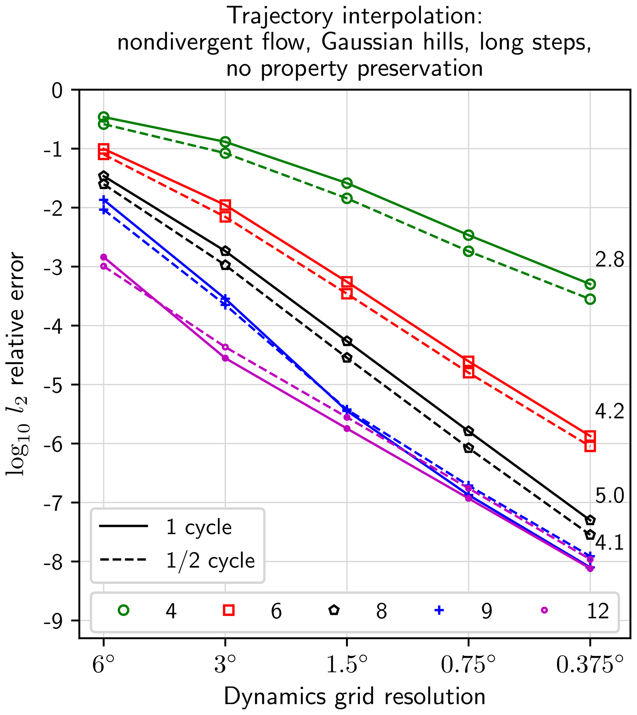
Figure 3 Comparison of relative errors calculated at the test simulation's midpoint time of 6 d ($\mathrm{1}/\mathrm{2}$ cycle, dashed lines) and endpoint time of 12 d (1 cycle, solid lines). Each number at the right side of the plot is the empirical OOA computed using the final two points of the one-cycle result.

Sometimes verification problems have unexpected features that interact with a method to produce higher-accuracy solutions than would occur in a more realistic problem. Of particular concern is the symmetry of the flow in time around the midpoint time, 6 d. To be sure our trajectory interpolation procedure is not interacting with this symmetry to produce artificially higher accuracy, in this experiment, we compute the solution error at the midpoint time as well as the final time.

The test uses the non-divergent flow, the Gaussian hills IC, and the long time step. The midpoint reference solution is computed using one 6 d step and the natural GLL basis. The time integrator's relative error tolerance is set to 10⁻¹⁴ rather than its usual 10⁻⁸ for this step. One remap step with the natural GLL basis provides a midpoint solution much more accurate than the time-stepped case, thus serving as an appropriate reference.

Figure 3 shows the results. The dashed curves show the errors measured at the midpoint, half of a cycle of the 12 d problem; the solid curves, the usual endpoint. The numbers at the right side of the plot show empirical OOA computed using the final two points of the one-cycle results. Numbers for the half-cycle curves are omitted because each pair of curves has almost exactly parallel lines for resolution at least as fine as 0.75^∘. In addition, the empirical OOA for $n_{\mathrm{p}}^{\mathrm{t}}=\mathrm{12}$ is omitted because the curves nearly overlap those for $n_{\mathrm{p}}^{\mathrm{t}}=\mathrm{9}$. For fine enough resolution, all curves should have empirical OOA limited to 4, but for $n_{\mathrm{p}}^{\mathrm{t}}=\mathrm{8}$, the full convergence regime is not reached in this plot, thus giving OOA 5 for $n_{\mathrm{p}}^{\mathrm{t}}=\mathrm{8}$. The $n_{\mathrm{p}}^{\mathrm{t}}=\mathrm{4}$ curves have OOA less than 4 due to a spatial OOA limit of 2 in the full convergence regime. We see OOA at about 4 for $n_{\mathrm{p}}^{\mathrm{t}}=\mathrm{9}$ and 12. The $n_{\mathrm{p}}^{\mathrm{t}}=\mathrm{9}$ curve shows at coarse resolution higher OOA, governed by the spatial error, and then a drop to 4 as the temporal error becomes dominant. Importantly, the half- and full-cycle errors are very close for each value of $n_{\mathrm{p}}^{\mathrm{t}}$, demonstrating that the endpoint error metrics are valid measurements for the Islet method.

4.1.2 Accuracy data for other standard configurations

The next figures show accuracy for standard configurations used in TR14. Although we explain how each figure can be compared with corresponding ones in TR14, these figures also stand on their own as simply convergence plots for various test cases.

Figure 4 Accuracy diagnostic. Compare with Figs. 1 and 2 in TR14.

Figure 5 Accuracy diagnostic. Compare with Figs. 1 and 2 in TR14.

Figure 6 Accuracy diagnostic. Compare with Fig. 3 in TR14.

Figure 7 Accuracy diagnostic. Compare with Fig. 3 in TR14.

Figure 8 Accuracy diagnostic. Compare with Fig. 16 in TR14.

Figure 9 Accuracy diagnostic. Compare with Fig. 16 in TR14.

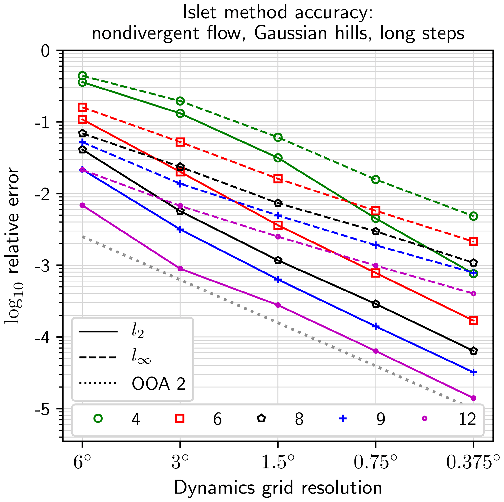
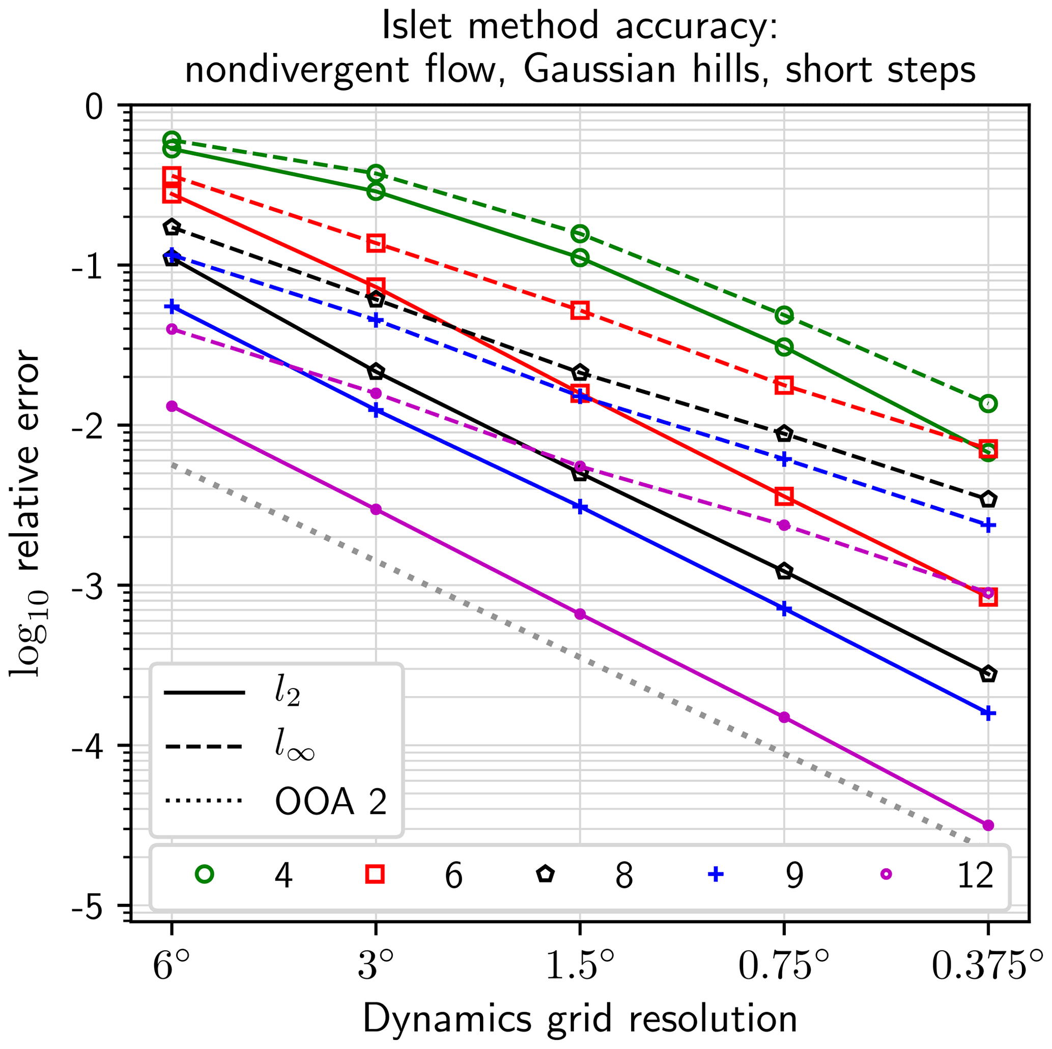
Figures 4 and 5 can be compared with Figs. 1 and 2 in TR14. They evaluate error on an infinitely smooth IC. The Islet method with a high-order basis compares extremely favorably with the methods in TR14. For example, the most accurate shape-preserving method in TR14 for the non-divergent flow with the Gaussian hills IC is the Hybrid Eulerian Lagrangian–Non-Diffusive (HEL-ND) method run with Courant number 1.0 (HEL-ND-CN1.0) by a substantial margin (cyan curves in Fig. 1, bottom right, of TR14). The $n_{\mathrm{p}}^{\mathrm{t}}=\mathrm{12}$ Islet scheme with the long time step, Fig. 4, is approximately three times more accurate than HEL-ND-CN1.0 in the l₂ norm at resolution 0.375^∘, and approximately twice as accurate at resolution 3^∘. Yet, HEL-ND is, quoting TR14, an “unphysical” method. It is run for comparison with the practically useful HEL scheme. After HEL-ND, the next most accurate method in the l₂ norm at 0.375^∘ resolution is CSLAM-CN5.0. The Islet method with the long time step, the same as that of CSLAM-CN5.0, is at least as accurate for $n_{\mathrm{p}}^{\mathrm{t}}\ge \mathrm{8}$. With the short time step, the same as that of CSLAM-CN1.0, the Islet method is at least as accurate as CSLAM-CN1.0 for $n_{\mathrm{p}}^{\mathrm{t}}\ge \mathrm{6}$. At 3^∘ resolution, no method other than HEL-ND-CN1.0 provides l₂ norm below 10⁻²; the Islet method does for $n_{\mathrm{p}}^{\mathrm{t}}\ge \mathrm{8}$ with the long time step, and $n_{\mathrm{p}}^{\mathrm{t}}\ge \mathrm{10}$ (only $n_{\mathrm{p}}^{\mathrm{t}}=\mathrm{12}$ is shown) with the short time step.

Now we must remind the reader that, in this article, we use nearly exact trajectories on the dynamics grid because the description of practical trajectory methods is outside the scope of this article. However, first, many of the schemes in TR14 use nearly exact trajectories, as well, e.g., CSLAM. Second, when using a practical trajectory algorithm, highly accurate, even if not exact, trajectories are possible because a trajectory over a tracer time step can be computed from multiple dynamics time steps. Thus, the use of exact trajectories is only slightly unrealistic. Third, the diagnostic values in Sect. 4.1.3, 4.1.4, and 4.3.2 are roughly independent of temporal errors.

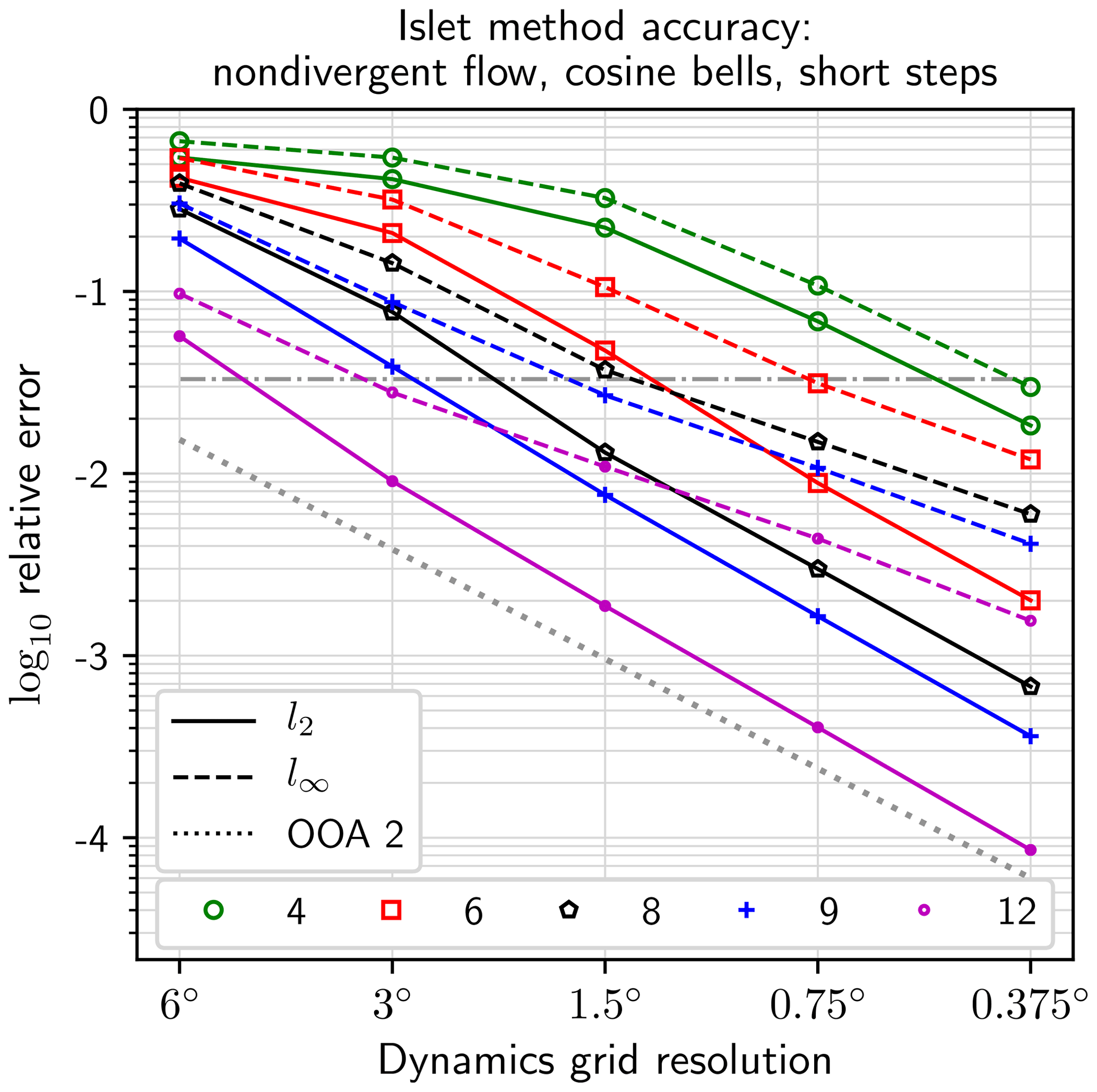
Figures 6 and 7 provide data that can be compared with the top panel of Fig. 3 in TR14. They evaluate error on a C¹ IC. The horizontal dash-dotted line provides the relative l₂-error-norm value of 0.033 by which the “minimal resolution” diagnostic value is determined; the coordinate of the intersection between the l₂-norm curve and this reference line is the value. A larger value is better. For example, with a long time step, for $n_{\mathrm{p}}^{\mathrm{t}}=\mathrm{8}$, this value is a little coarser than 3^∘; for $n_{\mathrm{p}}^{\mathrm{t}}=\mathrm{12}$, approximately 6^∘. For comparison, no model in TR14 reports a value larger than 2.5^∘.

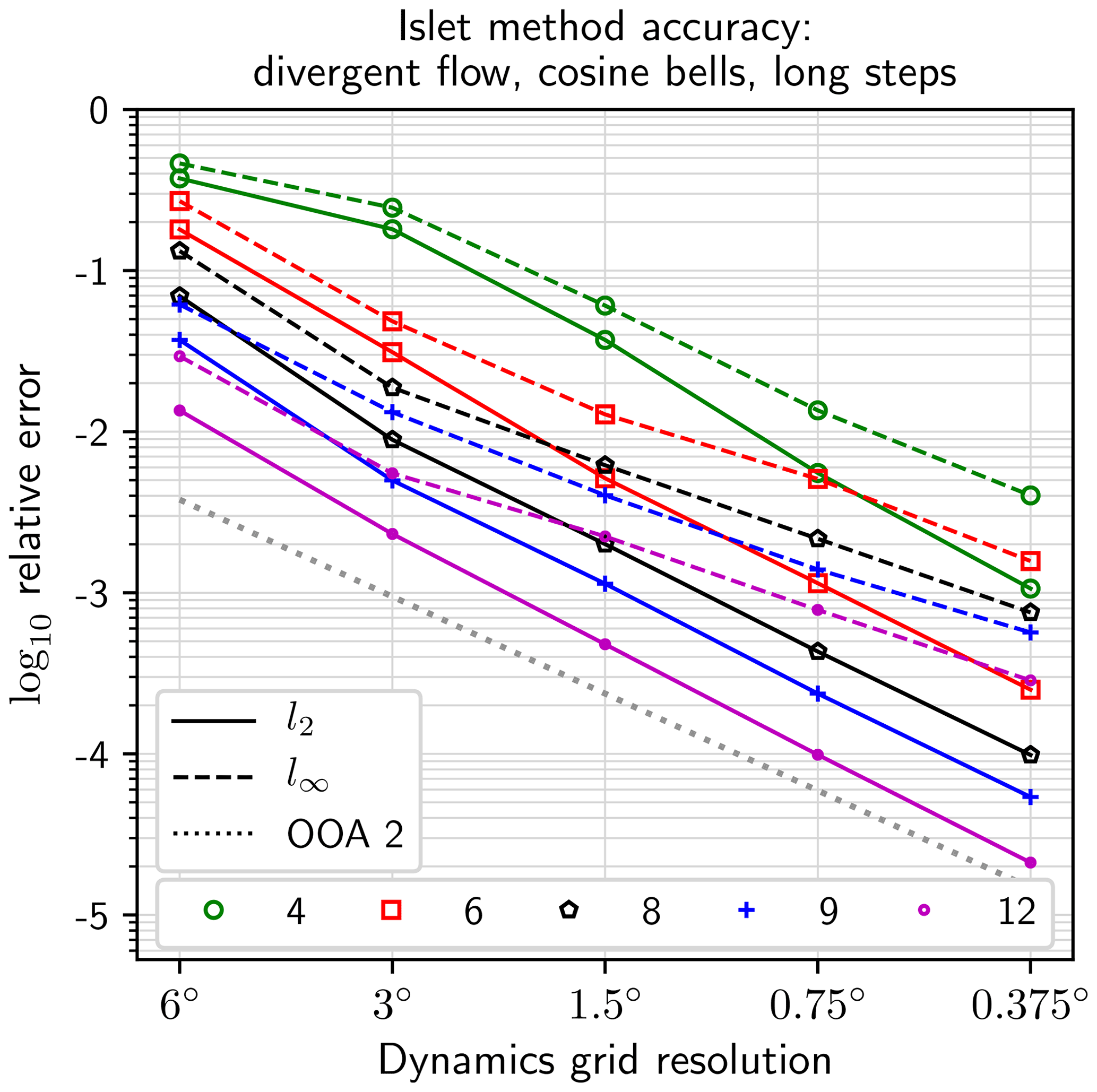
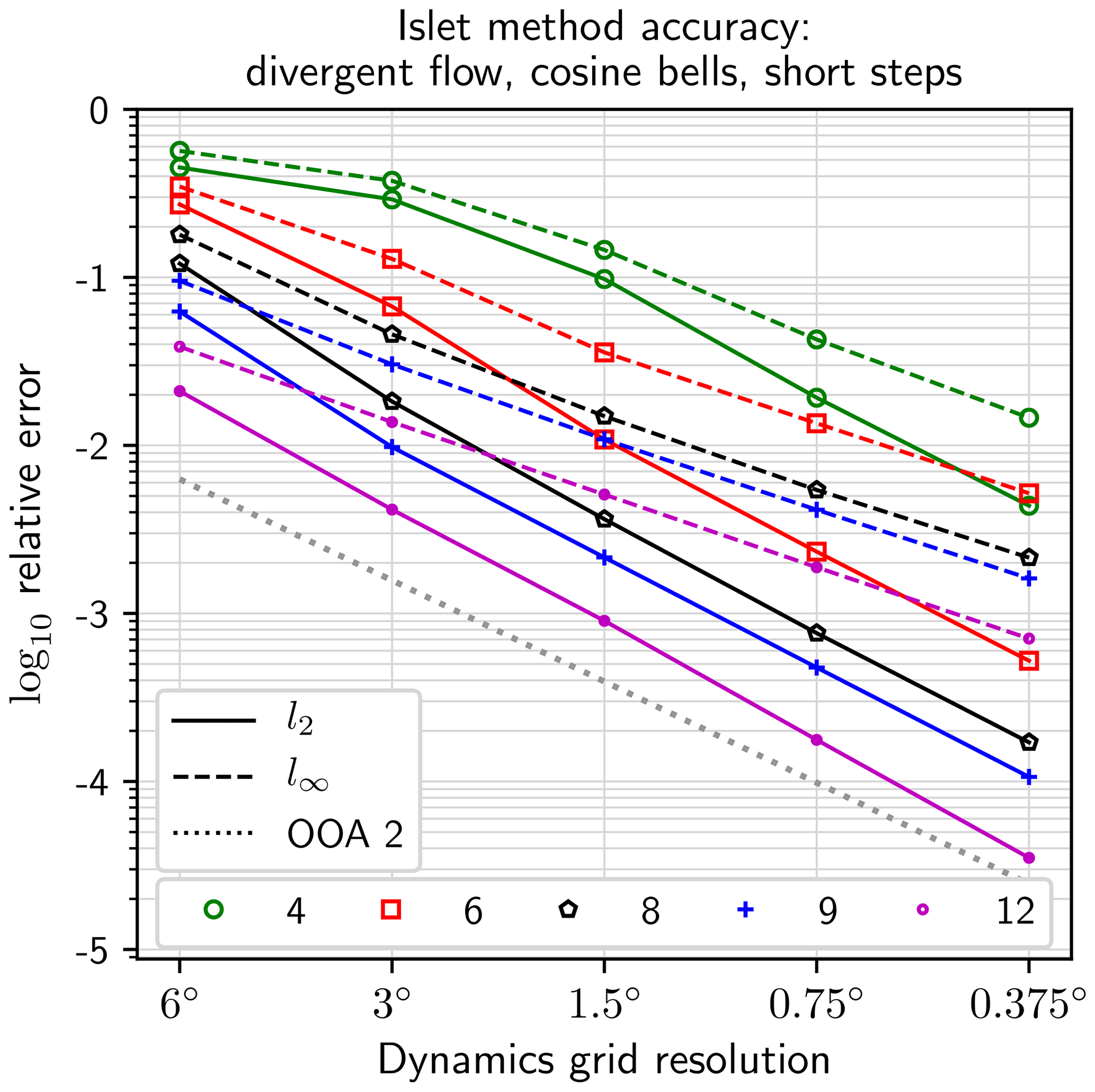
Figures 8 and 9 provide data that can be compared with the top two panels in Fig. 16 of TR14 given the minimum resolutions plotted in Fig. 3 of TR14. They are like Figs. 6 and 7 but, here, the divergent flow is used.

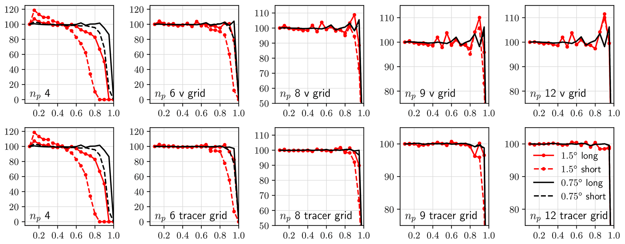
Figure 10 Filament diagnostic following Sect. 3.3 of TS12. Compare with Fig. 5 in TR14. The top row shows the diagnostic measured on the $n_{\mathrm{p}}^{\mathrm{v}}=\mathrm{4}$ dynamics grid; the bottom row on the tracer grid. The legend describes the dynamics-grid resolution and the time step length. The prescribed verification problem is the non-divergent flow with cosine bells IC. Property preservation is on. The x axis is τ, the mixing ratio threshold. The y axis is the percent area having mixing ratio at least τ relative to that at the initial time.

4.1.3 Filament diagnostic

Figure 10 shows results for the filament diagnostic described in Sect. 3.3 of TS12 to compare with Fig. 5 in TR14. The two dynamics grid resolutions are as prescribed in TR14. We used the code distributed with TS12 to compute the results. The diagnostic uses the non-divergent flow and the cosine bells IC. In this test, the midpoint solution is analyzed to determine the quality of the filamentary structure. See Fig. 13 for an illustration of the filamentary structure at the simulation midpoint, although with the slotted cylinders IC. For each possible value τ of the tracer mixing ratio at the initial time, the area over which the mixing ratio is at least τ at the midpoint time is computed. For the cosine bells IC, $\mathit{\tau }\in [\mathrm{0.1},\mathrm{1}]$. The diagnostic is then this area divided by the correct area, which for any non-divergent flow is the area at the initial time. The perfect diagnostic value is 100 % for all $\mathit{\tau }\in [\mathrm{0.1},\mathrm{1}]$ and 0 otherwise. In each plot in Fig. 10, the x axis is τ and the y axis is the diagnostic value. The diagnostic is computed for the dynamics-grid resolutions and time step lengths listed in the legend. Note that the y axis limits are tighter with increasing $n_{\mathrm{p}}^{\mathrm{t}}$.

A subtlety with this diagnostic is that the area calculation must use the quadrature method of the discretization. On the dynamics grid, the resulting curve is noisier than is implied by the underlying solution on the tracer grid. Thus, in Fig. 10, we show the diagnostic as computed on the dynamics grid in the top row of plots; on the tracer grid, in the bottom row.

There is no summary number that can be compared directly with the results in Fig. 5 of TR14, but, visually, the curves for $n_{\mathrm{p}}^{\mathrm{t}}\ge \mathrm{8}$, the resolution 1.5^∘, and on the tracer grid are among the best of those in TR14 at the resolution 1.5^∘.

4.1.4 Mixing diagnostic

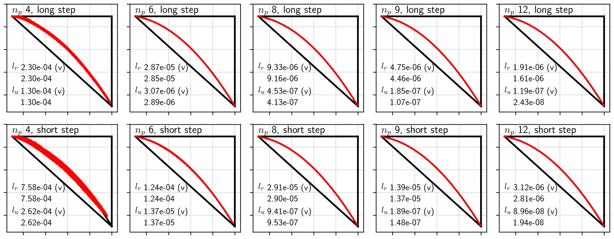
Figures 11 and 12 show results for the mixing diagnostics described in Sect. 3.5 of TS12 to compare with Figs. 11–14 in TR14. Again, the two dynamics grid resolutions are as prescribed in TR14.

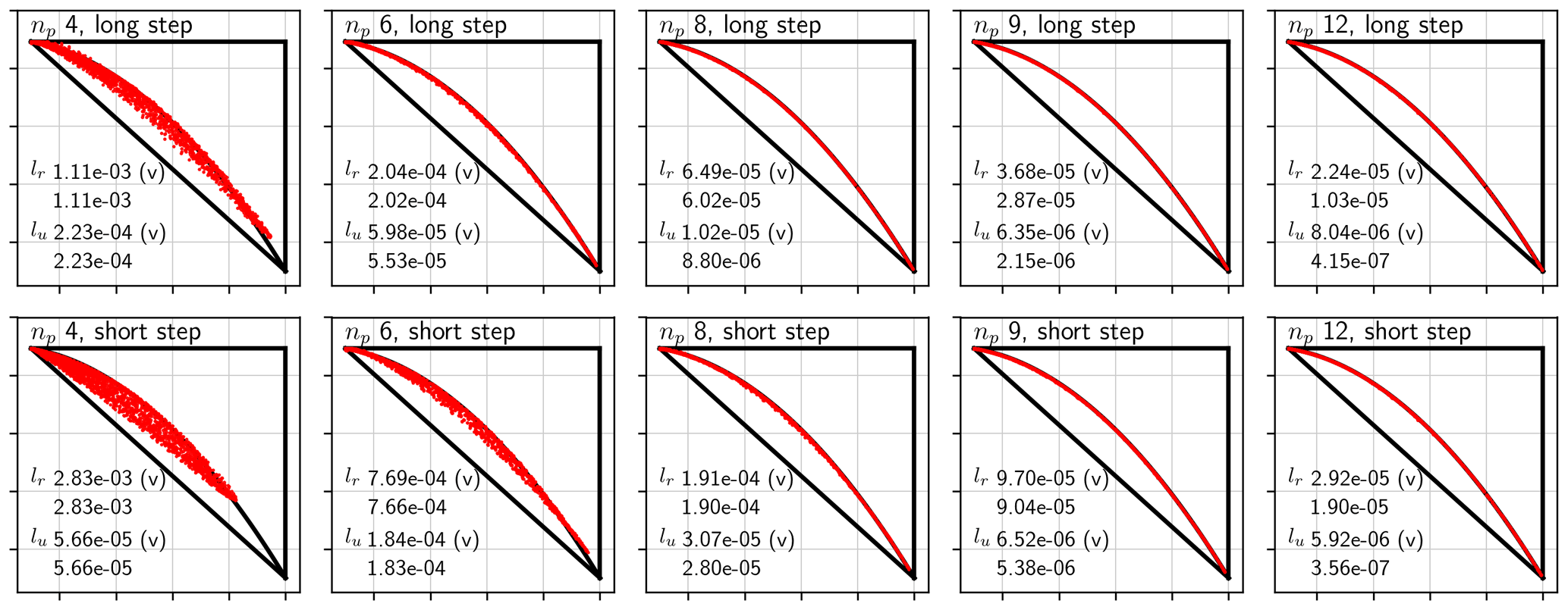
Figure 11 Mixing diagnostic following Sect. 3.5 of TS12. Compare with Figs. 11–14 in TR14. This figure shows results for dynamics-grid resolution of 1.5^∘. l_o is exactly 0 in all cases because shape preservation is on, and so is not shown. See text for further details.

Figure 12 Same as Fig. 11 but with dynamics-grid resolution 0.75^∘.

The test uses the non-divergent flow with two ICs. The diagnostics assess preservation of the nonlinear correlation of two tracers; one mixing ratio is a nonlinear function of the other. The mixing ratio of each tracer is on an axis, cosine bells on the x axis, and the correlated cosine bells field on the y axis. Each dot is a grid-point sample from the dynamics grid of the two mixing ratios. Like the filament diagnostic, the analysis is done at the solution midpoint rather than the endpoint. Also as for the filament diagnostic, we used the code distributed with TS12 to compute the results. $n_{\mathrm{p}}^{\mathrm{t}}$ and the time step length are printed in each plot. The diagnostic values l_r and l_u, explained in a moment, are also printed in each plot; the parenthesized “(v)” suffix means the value is measured on the dynamics grid, while the un-suffixed values are measured on the tracer grid.

At the initial time, all points are on the curve. Perfect nonlinear correlation corresponds to staying on the upper curve as the simulation proceeds. Points that drop into the convex hull of the starting points can be interpreted as physical mixing of air parcels, since such mixing results in a linear combination of two points on the curve. The diagnostic value l_r measures this type of error; smaller is better. In Figs. 11–14 in TR14, the smallest value of l_r at 1.5^∘ among the property-preserving methods is $\mathrm{2.15}\times {\mathrm{10}}^{-\mathrm{4}}$ by the University of California, Irvine, Second-Order Moments (UCISOM) method run with Courant number 5.5 (UCISOM-CN5.5), except for a value of 0 by HEL-ND, which, again, cannot be used in practice. For the long time step, the Islet method gives at least as small a value for $n_{\mathrm{p}}^{\mathrm{t}}\ge \mathrm{6}$; for the short time step, $n_{\mathrm{p}}^{\mathrm{t}}\ge \mathrm{8}$.

Values outside the triangle are overshoots, possible only if the method is not strictly shape preserving. Since our method is, this diagnostic value, l_o, is always 0, and is not displayed in the figures.

Values outside the convex hull cannot be described as physical mixing of parcels and, thus, are purely numerical artifacts of a method. The corresponding diagnostic is l_u and, again, smaller is better. This diagnostic is more difficult to compare than l_r because very dissipative methods tend to have a large value of l_r and, consequently, a very small value for l_u. In contrast, a very accurate method, for which l_r is small, can have a larger l_u value than a very dissipative method. One means of comparison is to consider the best l_u values among methods that obtain, say, $l_r\le \mathrm{5}\times {\mathrm{10}}^{-\mathrm{4}}$. In Figs. 11–14 in TR14, the smallest value of l_u at 1.5^∘ under this restriction is 0 obtained by the HEL-CN1.0 and HEL-CN5.5 methods. These HEL variants are practically usable unlike HEL-ND, and are designed to preserve tracer correlations exactly. Other than the HEL methods, the next best value is $\mathrm{4.80}\times {\mathrm{10}}^{-\mathrm{5}}$, again by the UCISOM-CN5.5 method. For both the long and short time steps, at 1.5^∘, the Islet method gives at least as small a value for $n_{\mathrm{p}}^{\mathrm{t}}\ge \mathrm{8}$. However, even with the constraint on l_r, comparison is not straightforward as the UCISOM methods are not strictly shape preserving and so have l_o>0.

4.2 Slotted cylinders

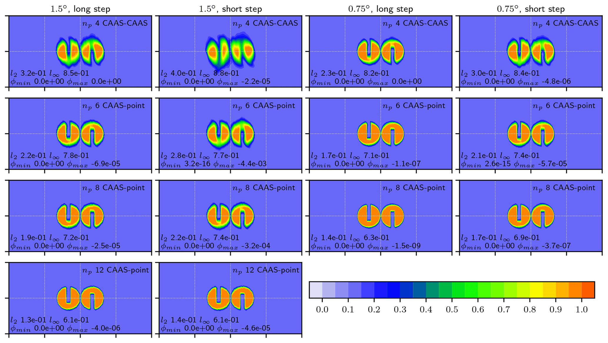
We observe that in both the filament and mixing diagnostics of TS12, $n_{\mathrm{p}}^{\mathrm{t}}\ge \mathrm{6}$ gives excellent results; $n_{\mathrm{p}}^{\mathrm{t}}=\mathrm{12}$, nearly perfect. Figures 13 and 14 show solution quality using latitude–longitude images and further underscore these observations. The problem is the non-divergent flow with the slotted cylinders IC, at resolutions 1.5 and 0.75^∘, with the long and short time steps. The text in the individual images in Fig. 14 provides normwise accuracy at the end of one cycle and deviation from the initial extrema. ${\mathit{\varphi }}_{min}\ge \mathrm{0}$ and ${\mathit{\varphi }}_{max}\le \mathrm{0}$ are consistent with no global extrema violation. Compare Fig. 13 with Figs. 7–10 in TR14 and both figures with Fig. 7 in TS12. Although TR14 does not provide error norm values for this problem, those in Fig. 7 of TS12 can be compared with the Islet method's values at 1.5^∘ resolution and the long time step (left column of Fig. 14). The Islet method's values of l₂, l_inf, ϕ_min, and ϕ_max are at least as good as those in Fig. 7 of TS12 for $n_{\mathrm{p}}^{\mathrm{t}}\ge \mathrm{6}$.

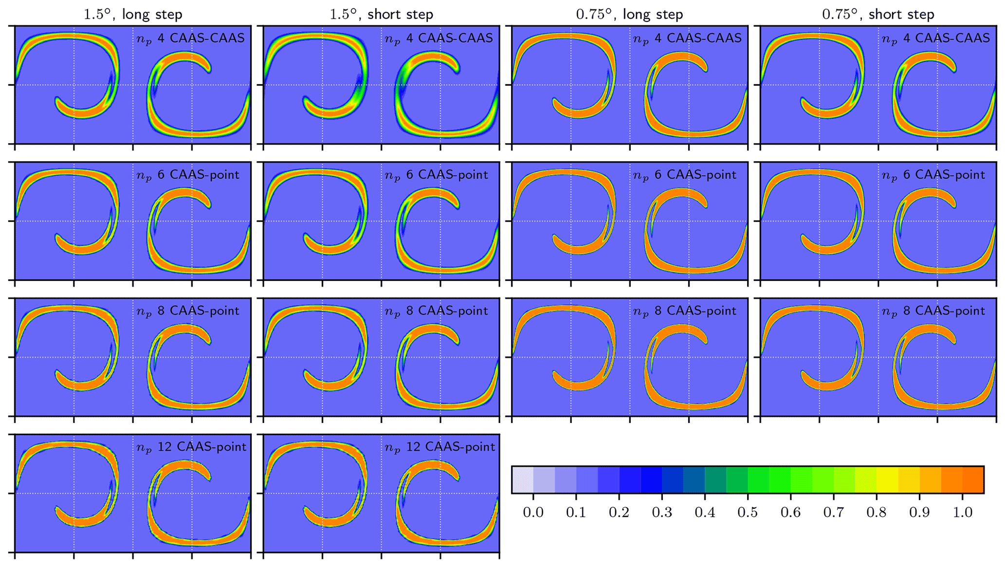
Figure 13 Images of the slotted cylinders IC advected by the non-divergent flow at the simulation's midpoint. Each column corresponds to a spatial resolution and time step length configuration, as stated at the top of each column. Each row corresponds to a particular value of $n_{\mathrm{p}}^{\mathrm{t}}$, as stated in the text at the top right of each image. We omit $n_{\mathrm{p}}^{\mathrm{t}}=\mathrm{12}$ results for the 0.75^∘ resolution because they are essentially identical at the resolution of the figure to the $n_{\mathrm{p}}^{\mathrm{t}}=\mathrm{8}$ images.

Figure 14 Same as Fig. 13 but for the simulation final point. Error measures are printed at the bottom left of each image; see text for details.

4.3 Source term

Now we move to verification problems that include a source term: f≠0 in Eq. (3).

4.3.1 Accuracy

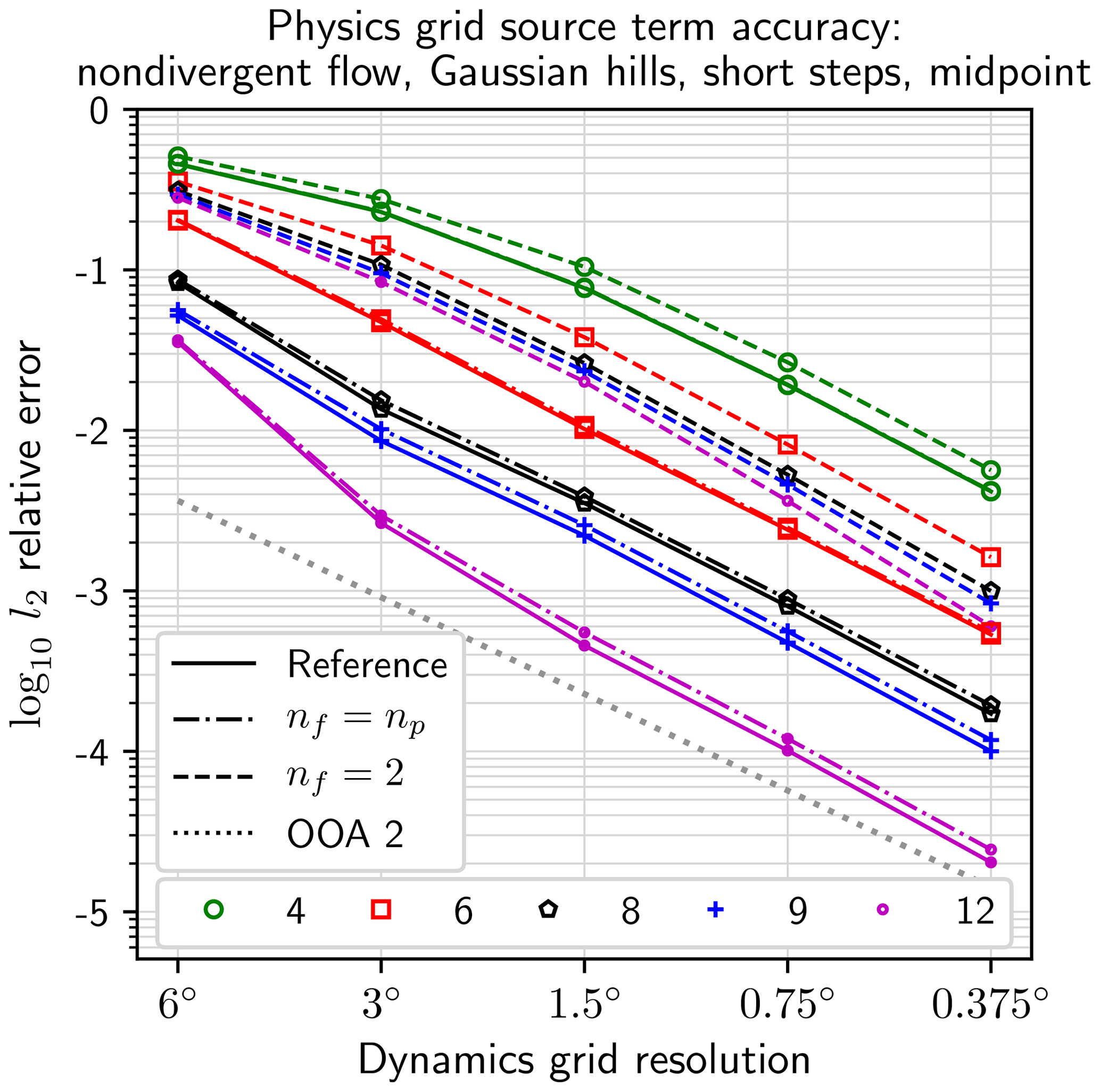
The first test verifies the property-preserving remaps between the physics and tracer grids. The test is constructed as follows. Two tracer mixing ratios, a source q₁=s and a manufactured tracer q₂=m, are paired. At time t=0, m(x,t) is set to 0, where x is position on the sphere. A tendency Δm is applied to m on the physics grid: $\mathrm{\Delta }m(\mathit{x},t)\equiv -\left[\cos \right(\mathrm{2}\mathit{\pi }(t+\mathrm{\Delta }t)/T)-\cos (\mathrm{2}\mathit{\pi }t/T\left)\right]s(\mathit{x},t)/\mathrm{2}$, so that the exact solution is $m(\mathit{x},t)=(\mathrm{1}-\cos (\mathrm{2}\mathit{\pi }t/T\left)\right)s(\mathit{x},t)/\mathrm{2}$ and, in particular, $m(\mathit{x},T/\mathrm{2})=s(\mathit{x},T/\mathrm{2})$. To compute the tendency, the state s(x,t) must be remapped to the physics grid. Thus, the results for this test depend on both grid-transfer directions. We measure the error at time $T/\mathrm{2}$, on the dynamics grid as usual, as in Fig. 3. Figure 15 shows the results. We run this test with $n_{\mathrm{f}}=n_{\mathrm{p}}^{\mathrm{t}}$ (dash-dotted lines) and n_f=2 (dashed lines). The solid lines show the error in $s(\mathit{x},T/\mathrm{2})$ as a reference. The dotted line provides the OOA-2 reference. We see that when $n_{\mathrm{f}}=n_{\mathrm{p}}^{\mathrm{t}}$, the errors are nearly the same as those for $s(\mathit{x},T/\mathrm{2})$; for $n_{\mathrm{p}}^{\mathrm{t}}=n_{\mathrm{f}}=\mathrm{4}$, the curves overlap at the resolution of the plot. As one expects, when n_f=2, the error in m(x,t) is much larger than in $s(\mathit{x},T/\mathrm{2})$, but the OOA remains 2.

Figure 15 Verification of the remap of tendencies from physics to tracer grids and state from tracer to dynamics grids. See Sect. 4.3 for a description of the problem.

4.3.2 Toy chemistry diagnostic

The toy chemistry verification problem is described in Lauritzen et al. (2015), subsequently TC15. The problem consists of two tracer mixing ratios, q_i=X_i, $i=\mathrm{1},\mathrm{2}$, that interact according to chemical kinetic equations that are nonlinear in one of them: $\mathrm{D}{X}_i(\mathit{y},t)/\mathrm{D}t=f_i(\mathit{y},X_{\mathrm{1}},X_{\mathrm{2}})$, where y is the spatial coordinate on the sphere. (We use y here to avoid overlap with the species symbol, X, that is used in TC15.) The tracers are composed of a monatomic and a diatomic molecule, respectively, of the same atomic species. The reactions are extremely sensitive to solar insolation. The sun's position is held fixed with respect to the grid. As a result, the largest-scale spatial pattern one sees in the fields is the boundary dividing nonzero (day) and zero (night) solar insolation, the solar terminator; this boundary is particularly visible in the right image of Fig. 17, a figure that we will describe subsequently. The ICs are designed so that the sum over the atomic mixing ratio at each point in space is a constant, ${\overline{X}}_T$. The source terms have this property too, since they model chemical reactions. Thus, in the exact solution, ${\overline{X}}_T$ is maintained at every point in space and time. Let X_T without a bar be the corresponding measured quantity. The toy chemistry diagnostics are then c₂(t), the l₂ norm of $X_T-{\overline{X}}_T$ at time t normalized by ${\overline{X}}_T$, and c_∞(t) the same but for the l_∞ norm.

As explained in the context of Eq. (14) in TC15, any advection operator that is semi-linear will produce a perfect diagnostic value of 0 when using exact arithmetic. Linear operators are semi-linear; the CEDR algorithms we use are as well, as explained in Bradley et al. (2019); and a composition of semi-linear operators is too. Thus, the Islet method is semi-linear, and deviation from 0 in the diagnostic values is wholly due to the effects of finite precision arithmetic.

We compute the diagnostics, as usual, on the dynamics grid. Following the Islet tracer transport method described in Sect. 3.1, the source terms are computed on the physics grid using states remapped from the tracer grid, and then the computed tendencies are remapped to the tracer grid.

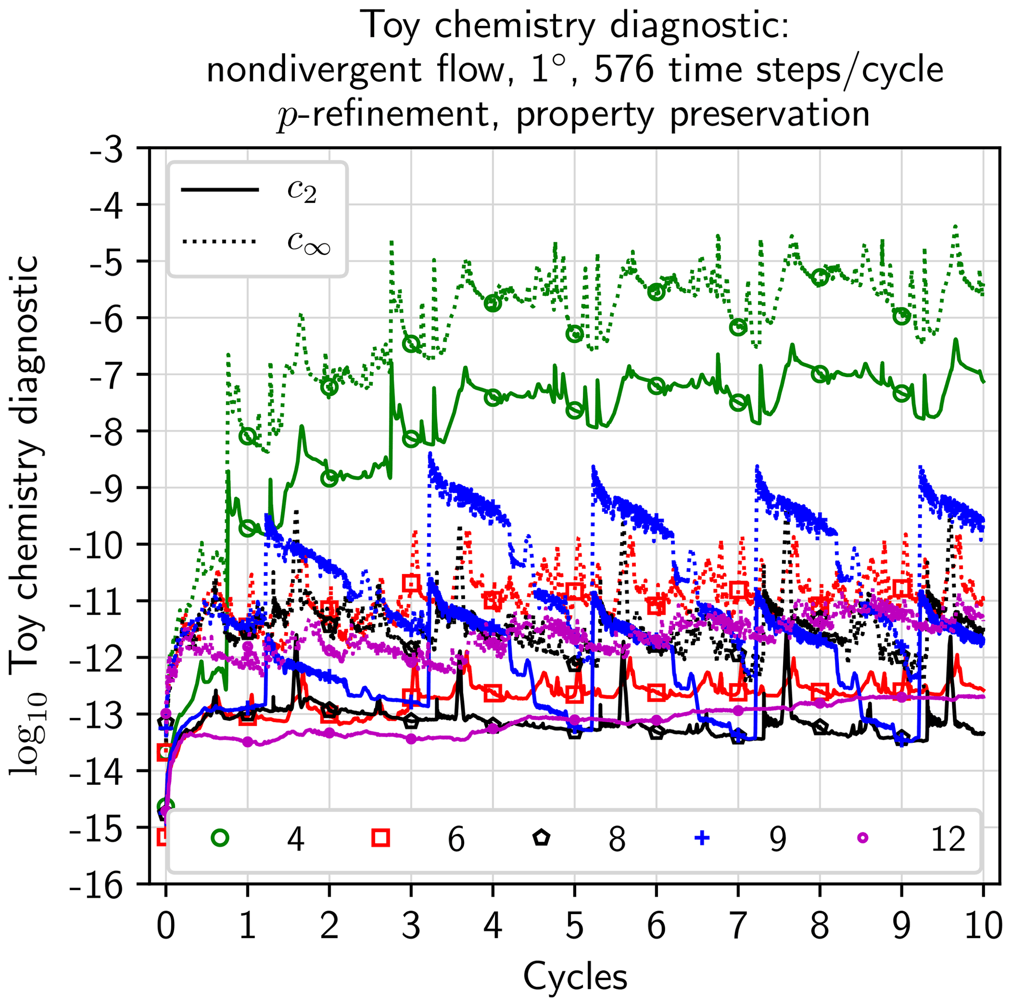
Figure 16 Toy chemistry diagnostic values as a function of time for 10 cycles of the non-divergent flow. Time is on the x axis and measured in cycles. Diagnostic values c₂ (solid lines) and c_∞ (dashed lines) are on the y axis. Markers as listed in the bottom legend are placed at the start of each cycle to differentiate the curves.

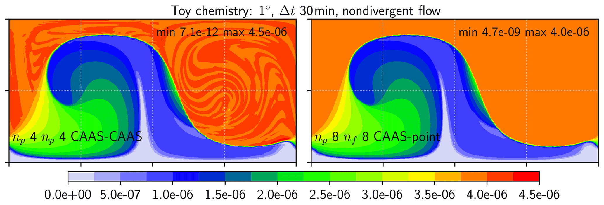
Figure 17 Images of the monatomic tracer at the end of the first cycle. Text at the lower left of each image states the configuration. Text at the upper right reports global extremal values.

Figure 18 Same as Fig. 17 but, now, the images are of $(X_T-{\overline{X}}_T)/{\overline{X}}_T$.

It is already known that the Eulerian spectral element tracer transport method yields poor values for this diagnostic due to finite-precision effects of the limiter (Lauritzen et al., 2017). The Islet method with property preservation using CAAS–CAAS does as well. Again, in exact arithmetic, each of these methods would produce perfect values. The poor diagnostic values are due to quickly accumulating machine-precision round-off errors that break semi-linearity in finite precision. The interaction of the chemistry source term with exact bounds in element-local limiter applications is responsible for this fast accumulation. In contrast, the Islet method using CAAS–point and relaxed-bound, element-local CAAS applications produces good diagnostic values. The relaxed bounds in the element-local part make unnecessary many of the mixing ratio adjustments that lead to loss of semi-linearity in finite precision. Recall that CAAS–point, applied at the end of the step, imposes the exact bounds, so at the end of a time step, shape preservation still holds to machine precision. Clips to bounds must still occur, but adjustments to other grid points to compensate are smaller because the adjustments are spread over many more grid points.

Figure 16 shows the diagnostic values for the case of non-divergent flow, 1^∘ dynamics-grid resolution, and a 30 min time step, where these configuration details are prescribed in TC15. For the $n_{\mathrm{p}}^{\mathrm{t}}=\mathrm{4}$ case, we use CAAS–point rather than CAAS–CAAS as previously, since we already know that CAAS–CAAS will produce poor values. The diagnostic is usually plotted over the course of one cycle (12 d) of the flow, but it is useful to view it over multiple cycles. Figure 16 shows 10 cycles on the x axis for a total of 120 d. The y axis is the diagnostic value. Solid lines plot c₂(t); dashed, c_∞(t). Markers are placed on the curves at the start of each cycle to differentiate the curves. In each case, $n_{\mathrm{f}}=n_{\mathrm{p}}^{\mathrm{t}}$. We choose this value of n_f because the toy chemistry source term has an extremely large gradient at the terminator and, thus, it makes sense to compute the physics tendencies at high spatial resolution. The $n_{\mathrm{p}}^{\mathrm{t}}=\mathrm{4}$ case with CAAS–point is greatly improved relative to the Eulerian spectral element results shown in Fig. 7 of TC15, even after 10 cycles instead of the one cycle shown in that figure. In Fig. 7 of TC15, $c_{\mathrm{2}}\approx {\mathrm{10}}^{-\mathrm{2}}$ and $c_{\mathrm{\infty }}>{\mathrm{10}}^{-\mathrm{1}}$ at the end of one cycle, compared with approximately 10⁻⁷ and 10⁻⁵, respectively, for $n_{\mathrm{p}}^{\mathrm{t}}=\mathrm{4}$ at the end of 10 cycles. For $n_{\mathrm{p}}^{\mathrm{t}}>\mathrm{4}$, the growth in error is very small, with $c_{\mathrm{2}}<{\mathrm{10}}^{-\mathrm{10}}$ through 10 cycles.

To illustrate what these diagnostics measure, Fig. 17 shows latitude–longitude images of the monatomic tracer at the end of the first cycle for $n_{\mathrm{p}}^{\mathrm{t}}=n_{\mathrm{f}}=\mathrm{4}$ with CAAS–CAAS (left) and $n_{\mathrm{p}}^{\mathrm{t}}=n_{\mathrm{f}}=\mathrm{8}$ with CAAS–point (right). Note that the images in TS12 and TR14 are plotted with longitude ranging from 0 to 2π; those in TC15, from −π to π. In our latitude–longitude figures so far, we have chosen the convention used in TS12 and TR14, and we continue to use it in these toy-chemistry images. Thus, these images are circularly shifted horizontally by half the image width relative to those in TC15. The globally extremal tracer values are printed in the upper right quadrant of each image. The correct maximum is $\mathrm{4}\times {\mathrm{10}}^{-\mathrm{6}}$ and the correct minimum is at least 0. The right image is free of noise and satisfies these bounds. The left image shows substantial noise, as we expect when using exact bounds in the local property preservation problems, and consistent with previous observations about spectral element transport. Other than noise and some filaments that grow from the noise, the two images are qualitatively similar. Figure 18 shows images in the same format, but the quantity is now $(X_T-{\overline{X}}_T)/{\overline{X}}_T$ at the end of the first cycle. The correct value is 0 everywhere. In the right image, the pointwise relative error is a little better than 10⁻¹¹, consistent with the l_∞-norm diagnostic value for $n_{\mathrm{p}}^{\mathrm{t}}=\mathrm{8}$ at the end of the first cycle in Fig. 16.

5 Conclusions

We described the Islet method, a property-preserving tracer transport method to support a three-grid atmosphere model, one with a shared element grid but separate subelement grids for physics parameterizations, dynamics, and tracer transport. This configuration permits the modeler to create a dynamics grid with a tolerable CFL-limited time step independent of the other two subcomponents, while physics parameterizations and tracer transport can run at resolutions potentially substantially higher. The shared element grid minimizes communication during remaps between grids, and almost all operations are local to each element, making the Islet method extremely efficient.

Section 4 presented a number of verification problems with diagnostics assessing accuracy, order of accuracy, numerical mixing, filament preservation, and nonlinear correlation preservation. The corresponding figures and diagnostic values can be compared directly with those of several other methods. The Islet method performs well in a number of detailed comparisons.

Possible future work includes the following. First, because all operations except the DSS are either local to the element or act on element-level scalars, both the tracer and the physics grids permit various types and subsets of spatially and temporally adaptive and tracer-dependent refinement and derefinement, possibly in combination with already existing E3SM regionally refined models (RRM). Future work could develop procedures to permit spatially and temporally varying $n_{\mathrm{p}}^{\mathrm{t}}$ and n_f values, and incorporate these into the Islet method.

Second, this article focuses on the horizontal dimensions or, more generally, 2D Lagrangian levels in a three-dimensional discretization. However, it is necessary to increase simultaneously both the horizontal and vertical resolutions of a plume to capture and maintain its structure (Eastham and Jacob, 2017). Future work using methods similar to those in Sect. 3 should address the vertical dimension.

Third, it is possible to recover local mass conservation in an ISL method by modifying the linear advection operator's coefficients so that the sum of the mass over all the target points associated with a source element is consistent with the source element's total mass (Kaas, 2008). This coefficient modification step might be compatible with the Islet method and should be explored.

Finally, we predict that applications related to, in particular, aerosols will benefit from the Islet method. In future work, we intend to integrate the Islet method into the E3SM Atmosphere Model to investigate its impact on science applications.

Appendix A: Islet bases

The GLL basis functions yield an unstable ISL method for n_p≥4. We developed a set of bases on GLL nodes that yield ISL methods that meet a necessary condition for stability on the test problem of uniform periodic flow. We refer to these as the Islet bases and use these bases in this article. Bradley et al. (2021, Sects. 2 and 3) and a forthcoming article based on that material detail the derivation of the Islet bases, while this appendix summarizes the results of that derivation for completeness. This article can be understood equally well by assuming the standard GLL bases are used; only the numerical results depend on the details of the basis functions.

A 1D reference element has domain $[-\mathrm{1},\mathrm{1}]$. Higher-dimensional basis functions are tensor products of 1D basis functions. The bases are nodal, meaning a basis function has the value 1 at one node and 0 at all others. The nodes are GLL. Let $x_G^{n_{\mathrm{p}}}\left(i\right)$, $i\in \mathit{\{}\mathrm{0},\mathrm{\dots },n_{\mathrm{p}}-\mathrm{1}\mathit{\}}$, be the reference coordinates of the GLL nodes. Let region $r\in \mathit{\{}\mathrm{0},\mathrm{\dots },n_{\mathrm{p}}-\mathrm{2}\mathit{\}}$ be the segment $\left[x_G^{n_{\mathrm{p}}}\right(r),x_G^{n_{\mathrm{p}}}(r+\mathrm{1}\left)\right]$. A 1D basis function is a continuous piecewise polynomial over $[-\mathrm{1},\mathrm{1}]$; in each region, it is a polynomial. Each region r has an associated ordered list of support nodes, denoted ${\mathcal{I}}_r^{n_{\mathrm{p}}}$. Each list ${\mathcal{I}}_r^{n_{\mathrm{p}}}$ is a subset of $\mathit{\{}\mathrm{0},\mathrm{\dots },n_{\mathrm{p}}-\mathrm{1}\mathit{\}}$. Let $\left|{\mathcal{I}}_r^{n_{\mathrm{p}}}\right|$ be the number of elements in ${\mathcal{I}}_r^{n_{\mathrm{p}}}$, let $n_{\mathrm{p}}^{\mathrm{submin}}\equiv {min}_r\left|{\mathcal{I}}_r^{n_{\mathrm{p}}}\right|$, and let ${\mathcal{I}}_r^{n_{\mathrm{p}}}\left(j\right)$ be the jth element.

In region r and thus for $x\in \left[x_G^{n_{\mathrm{p}}}\right(r),x_G^{n_{\mathrm{p}}}(r+\mathrm{1}\left)\right]$, basis function k is 0 if $k\notin {\mathcal{I}}_r^{n_{\mathrm{p}}}$ and otherwise has the value given by the Lagrange polynomial

$${\mathit{\varphi }}_k^{n_{\mathrm{p}}}\left(x\right)\equiv \prod _{\begin{array}{c}j\in \mathit{\{}\mathrm{0},\mathrm{\dots },|{\mathcal{I}}_r^{n_{\mathrm{p}}}|-\mathrm{1}\mathit{\}},\\ {\mathcal{I}}_r^{n_{\mathrm{p}}}\left(j\right)\ne k\end{array}}{\displaystyle \frac{x-x_G^{n_{\mathrm{p}}}\left({\mathcal{I}}_r^{n_{\mathrm{p}}}\right(j\left)\right)}{x_G^{n_{\mathrm{p}}}\left(k\right)-x_G^{n_{\mathrm{p}}}\left({\mathcal{I}}_r^{n_{\mathrm{p}}}\right(j\left)\right)}}.$$

We construct a basis for each $n_{\mathrm{p}}\in \mathit{\{}\mathrm{4},\mathrm{\dots },\mathrm{13}\mathit{\}}$. Each basis is described by a set of support node lists, one ${\mathcal{I}}_r^{n_{\mathrm{p}}}$ per region. For n_p=4, there are additional details that we describe in Appendix A1. There are two types of bases, each corresponding to a method of describing the support node lists.

The first type of basis is the offset nodal basis. Each list ${\mathcal{I}}_r^{n_{\mathrm{p}}}$ is given by an offset, which is the first index in the list and its size, $\left|{\mathcal{I}}_r^{n_{\mathrm{p}}}\right|$. For example, n_p=7, offset 2, and size 4 correspond to support nodes ${\mathcal{I}}_r^{\mathrm{7}}=\mathit{\{}\mathrm{2},\mathrm{3},\mathrm{4},\mathrm{5}\mathit{\}}$. In addition, the basis is symmetric, meaning basis function ${\mathit{\varphi }}_i^{n_{\mathrm{p}}}\left(x\right)={\mathit{\varphi }}_{n_{\mathrm{p}}-\mathrm{1}-i}^{n_{\mathrm{p}}}(-x)$. Thus, first, support nodes are specified for regions 0 through $\lfloor n_{\mathrm{p}}/\mathrm{2}\rfloor -\mathrm{1}$, and the support nodes for the remaining regions are determined by symmetry. Second, if n_p is even, then the middle region, $r=n_{\mathrm{p}}/\mathrm{2}-\mathrm{1}$, has support nodes ${\mathcal{I}}_r^{n_{\mathrm{p}}}$ that are symmetric around reference coordinate 0.

The second type of basis is the nodal basis. An offset nodal basis is a nodal basis whose support nodes all permit the more compact description of offset and size. A general nodal basis has at least one support nodal list that cannot be described by just an offset and a size. Instead, the list is stated explicitly. Again, all nodal bases are symmetric.

The order of accuracy of the ISL method using an Islet GLL basis is $n_{\mathrm{p}}^{\mathrm{submin}}-\mathrm{1}$ if there is no property preservation step and the initial condition is $C^{n_{\mathrm{p}}^{\mathrm{submin}}-\mathrm{2}}$.

If $n_{\mathrm{p}}^{\mathrm{submin}}=n_{\mathrm{p}}$, then the basis is the natural GLL basis. Thus, any statement about an Islet GLL basis also holds for the natural GLL basis.

A search procedure searches for nodal bases that provide ISL methods that are stable on the test problem of uniform flow on a uniform grid. An accuracy heuristic is used to find the most accurate basis satisfying this stability condition. Table A1 lists nodal bases, most of them offset nodal bases, for $n_{\mathrm{p}}\in \mathit{\{}\mathrm{5},\mathrm{\dots },\mathrm{13}\mathit{\}}$. In addition, a special basis is constructed for n_p=4.

Table A1 Islet GLL nodal subset bases. Each row provides a formula for the row's n_p value. Columns are n_p, order of accuracy (OOA), the support sizes $\left|{\mathcal{I}}_r\right|$ for each region ordered left to middle, and the supports. For offset nodal subset bases, supports are given by offsets. For general nodal subset bases, supports are given by nodal subsets, again ordered from left region to middle. The case n_p=4 is described in Appendix A1. In all cases, the support points are GLL nodes.

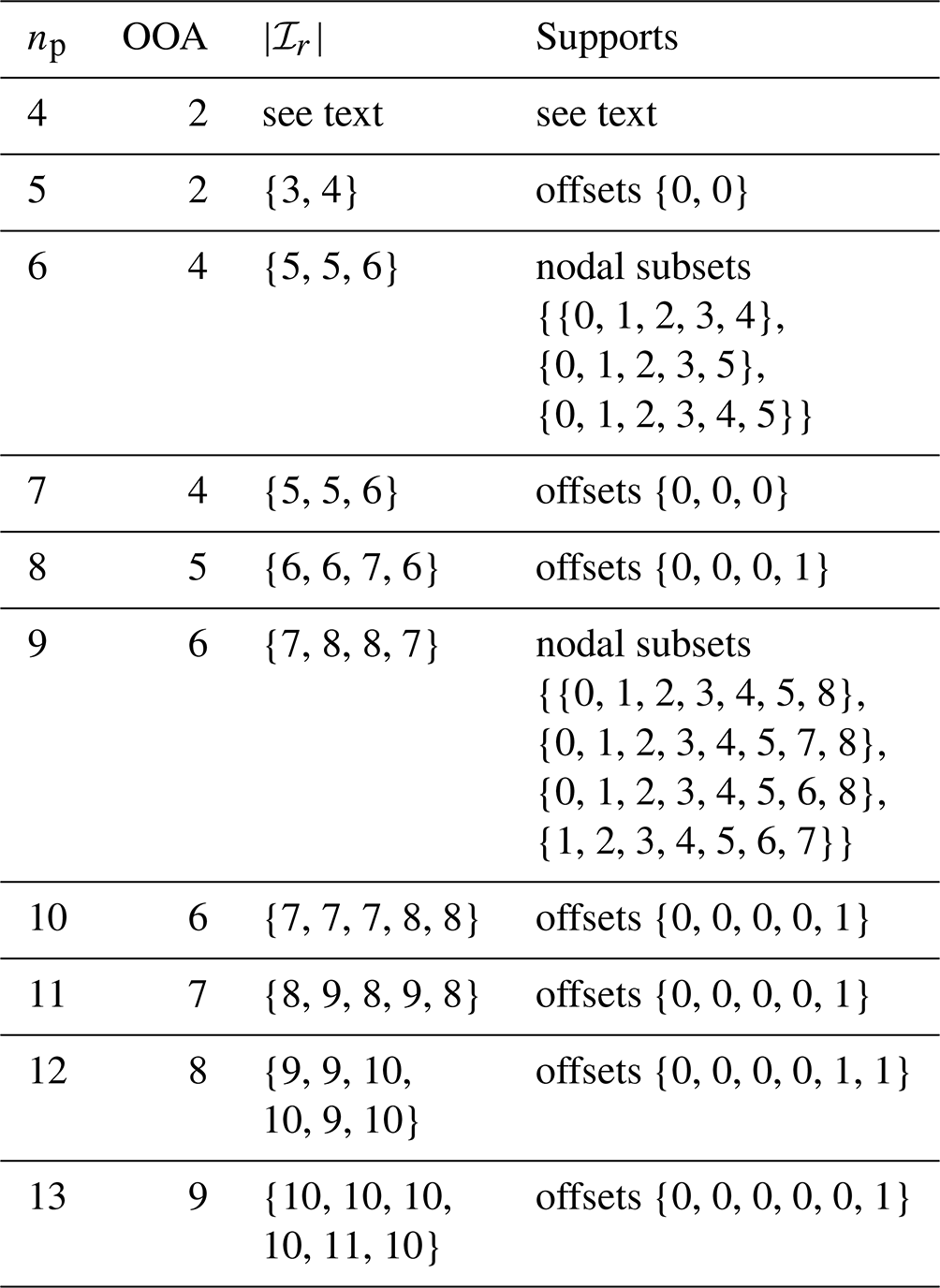
A1 n_p=4 Islet basis

For n_p=4, we boost the accuracy of the basis by combining an offset nodal basis and the GLL basis. The middle region has support nodes ${\mathcal{I}}_{\mathrm{1}}=\mathit{\{}\mathrm{0},\mathrm{1},\mathrm{2},\mathrm{3}\mathit{\}}$, i.e., all four nodes. Region 0 convexly combines basis function k given by ${\mathcal{I}}_{\mathrm{0}}^{\mathrm{4}}=\mathit{\{}\mathrm{0},\mathrm{1},\mathrm{2}\mathit{\}}$ with GLL basis function k over the region $x\in \left[x_G^{\mathrm{4}}\right(\mathrm{0}),x_G^{\mathrm{4}}(\mathrm{1}\left)\right]$, with convex combination function α(x). α(x) is a quadratic polynomial having values 1, 0.306, and 0 at, respectively, the left side, middle, and right side of region 0. The combination is defined so that at the left side, where $\mathit{\alpha }(-\mathrm{1})=\mathrm{1}$, only the GLL basis function k is used; at the right side, where $\mathit{\alpha }\left(x_G^{\mathrm{4}}\right(\mathrm{1}\left)\right)=\mathrm{0}$, only the offset nodal basis function k is used. Region 2 is constructed by symmetry. α(x) is determined to maximize the accuracy of the resulting ISL method subject to the constraint of stability on the test problem.

A2 Conservation when interpolating

The element-local conservation expressed in Eq. (15) holds for the following reasons. First, for any Islet basis for which $(n_{\mathrm{p}}^{\mathrm{t}}{)}^{\mathrm{submin}}\ge n_{\mathrm{p}}^{\mathrm{v}}$, the continuum field f is the same on each grid, since the tracer grid can exactly represent polynomials of degree $n_{\mathrm{p}}^{\mathrm{v}}-\mathrm{1}$. Second, for $n_{\mathrm{p}}^{\mathrm{v}}$ even, such as the standard $n_{\mathrm{p}}^{\mathrm{v}}=\mathrm{4}$, if $(n_{\mathrm{p}}^{\mathrm{t}}{)}^{\mathrm{submin}}=n_{\mathrm{p}}^{\mathrm{v}}-\mathrm{1}$, the continuum field f is, in general, different on each grid, but the integral of each over an element has the same value. This is because for polynomial degree d odd and $f\left(x\right)\equiv {\sum }_{i=\mathrm{0}}^d{a}_i{x}^i$, ${\int }_{-\mathrm{1}}^{\mathrm{1}}f\left(x\right)\mathrm{d}x$ = ${\int }_{-\mathrm{1}}^{\mathrm{1}}\left(f\right(-x)+f(x\left)\right)/\mathrm{2}\mathrm{d}x$, and $g\left(x\right)\equiv \left(f\right(-x)+f(x\left)\right)/\mathrm{2}$ has degree at least one less than f(x). g(x) is exactly represented on the tracer grid and, thus, the integral of f, which is the same as the integral of g, is the same on the tracer grid as on the dynamics grid. These two reasons assure that ℐ^v→t is conservative for the Islet bases in Table A1 when $n_{\mathrm{p}}^{\mathrm{v}}=\mathrm{4}$.

A3 Unstable and stable integration

Figure A1, which has the format of the figures described in Sect. 4, compares accuracy and stability between the natural and Islet bases. The divergent flow, Gaussian hills IC, property preservation, TTPR, and long time steps are used. To test the stability of the ISL linear advection operator using the Islet bases, we run the verification problem for both 1 cycle and 100 cycles. A curve's line pattern corresponds to basis type and number of cycles: solid, Islet basis for 1 cycle; dashed, Islet basis for 100 cycles (or $\mathrm{12}\times \mathrm{100}=\mathrm{1200}$ d); dash-dotted, natural basis for 1 cycle. For each $n_{\mathrm{p}}^{\mathrm{t}}$, the l₂ norm of the solution using the natural basis diverges with increasing resolution within the first cycle, demonstrating that the basis leads to an unstable ISL linear advection operator. In the case of $n_{\mathrm{p}}^{\mathrm{t}}=\mathrm{4}$, we see the start of the curve's divergence, but further element-grid refinement is needed to see the curve fully diverge. In contrast, the curves for the Islet method with the Islet bases converge at order of accuracy 2.

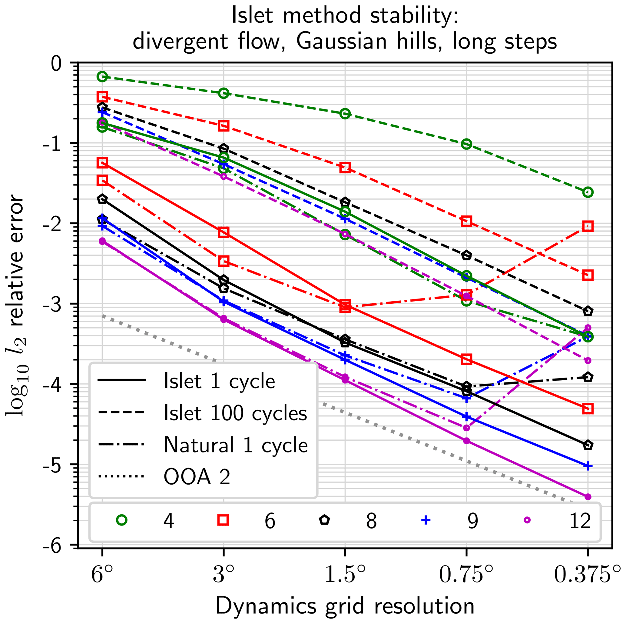
Figure A1 Stability of the Islet method with the Islet GLL bases compared with the instability of the method with the natural GLL bases. The x axis is the average dynamics-grid grid point spacing at the equator in degrees for the quasiuniform cubed-sphere grid. The y axis is log ₁₀l₂ relative error. A curve's line pattern corresponds to the basis type and number of cycles, as listed in the top legend. A curve's marker corresponds to $n_{\mathrm{p}}^{\mathrm{t}}$, as listed in the bottom legend.

Appendix B: Discretization of the continuity equation

Our primary interest is the advection equation and not the continuity equation. However, to run tests with divergent flow and property preservation enabled, we need to solve the continuity equation for the air density to provide the ρ argument to CAAS. This appendix describes a discretization of the continuity equation that differs in only one factor from the discretization of the advection equation.

We start by following, e.g., Giraldo (1997, Sect. 3.3) and Bosler et al. (2019, Sect. 3). The Reynolds transport theorem for a Lagrangian fluid parcel Ω(t) containing a fluid having density ρ(x,t) is

$$\begin{array}{}\text{(B1)}& {\displaystyle \frac{\mathrm{d}}{\mathrm{d}t}}\underset{\mathrm{\Omega }\left(t\right)}{\int }\mathit{\rho }\mathrm{d}\mathit{x}=\underset{\mathrm{\Omega }\left(t\right)}{\int }{\mathit{\rho }}_t+\mathrm{\nabla }\cdot \left(\mathit{\rho }\mathit{u}\right)\mathrm{d}\mathit{x}.\end{array}$$

To balance clarity and concision, we include or omit the position and time arguments depending on the context. Suppose ρ satisfies the continuity equation,

$$\begin{array}{}\text{(B2)}& {\mathit{\rho }}_t+\mathrm{\nabla }\cdot \left(\mathit{\rho }\mathit{u}\right)=\mathrm{0}.\end{array}$$

In addition, consider a function ϕ(x,t) that satisfies the advection equation,

$$\begin{array}{}\text{(B3)}& {\displaystyle \frac{\mathrm{D}\mathit{\varphi }}{\mathrm{D}t}}=\mathrm{0}.\end{array}$$

Then, by Eqs. (B1), (B2), and (B3),

$$\begin{array}{ll}{\displaystyle \frac{\mathrm{d}}{\mathrm{d}t}}\underset{\mathrm{\Omega }\left(t\right)}{\int }\mathit{\rho }\mathit{\varphi }\mathrm{d}\mathit{x}& {\displaystyle }=\underset{\mathrm{\Omega }\left(t\right)}{\int }(\mathit{\rho }\mathit{\varphi }{)}_t+\mathrm{\nabla }\cdot (\mathit{\rho }\mathit{\varphi }\mathit{u})\mathrm{d}\mathit{x}\\ {\displaystyle }& {\displaystyle }=\underset{\mathrm{\Omega }\left(t\right)}{\int }\mathit{\varphi }[{\mathit{\rho }}_t+\mathrm{\nabla }\cdot (\mathit{\rho }\mathit{u}\left)\right]+\mathit{\rho }{\displaystyle \frac{D\mathit{\varphi }}{\mathrm{D}t}}\mathrm{d}\mathit{x}\\ {\displaystyle }& {\displaystyle }=\mathrm{0},\end{array}$$

which, in turn, implies

$$\begin{array}{}\text{(B4)}& \underset{\mathrm{\Omega }\left(t_{\mathrm{1}}\right)}{\int }\mathit{\rho }\mathit{\varphi }\mathrm{d}\mathit{x}=\underset{\mathrm{\Omega }\left(t_{\mathrm{0}}\right)}{\int }\mathit{\rho }\mathit{\varphi }\mathrm{d}\mathit{x}\end{array}$$

for all times t₀, t₁.

Now we discretize Eq. (B4) in space. First, we write an integral over a scalar f in terms of the element reference coordinate system. Let Ω(t) be a quadrilateral element, with Ω(t₁) the arrival Eulerian element. Then,

$$\begin{array}{}\text{(B5)}& \underset{\mathrm{\Omega }\left(t\right)}{\int }f(\mathit{x},t)\mathrm{d}\mathit{x}=\underset{-\mathrm{1}}{\overset{\mathrm{1}}{\int }}\underset{-\mathrm{1}}{\overset{\mathrm{1}}{\int }}f\left(\mathit{x}\right(\mathit{r},t),t)J(\mathit{r},t)\mathrm{d}\mathit{r}.\end{array}$$

Here, $\mathit{x}(\mathit{r},t)\equiv \mathit{X}(t;\mathit{x}(\mathit{r},t_{\mathrm{1}}),t_{\mathrm{1}})$ is the time-dependent map from the reference element to the manifold, and satisfies Eq. (6). J(r,t) is the absolute value of the Jacobian determinant of this map, $\left|\det \right(\partial \mathit{x}(\mathit{r},t)/\partial \mathit{r}\left)\right|$.

Second, let the element have a tensor-product grid of GLL nodes, with n_p the number of 1D nodes. We apply tensor-product GLL quadrature with this value of n_p to the right hand side of Eq. (B5). Then,

$$\begin{array}{ll}{\displaystyle }\underset{-\mathrm{1}}{\overset{\mathrm{1}}{\int }}\underset{-\mathrm{1}}{\overset{\mathrm{1}}{\int }}& {\displaystyle }f\left(\mathit{x}\right(\mathit{r},t),t)J(\mathit{r},t)\mathrm{d}\mathit{r}\\ {\displaystyle }& {\displaystyle }\approx \sum _{i=\mathrm{0}}^{n_{\mathrm{p}}^{\mathrm{2}}-\mathrm{1}}f\left(\mathit{x}\right({\mathit{r}}_i,t),t)J({\mathit{r}}_i,t)w_i,\end{array}$$

where i iterates over nodes in the element, r_i is the ith GLL node, and w_i is the ith GLL weight. Let ${\mathit{x}}_i\left(t\right)\equiv \mathit{x}({\mathit{r}}_i,t)$.

Third, we combine the quadrature approximation with a specific form of f, f=ρϕ, where ϕ satisfies Eq. (B3). Let ϕ(x,t₁) be an element, GLL nodal, tensor-product n_p-basis function on an Eulerian arrival element. Because ϕ is a nodal basis function with the same nodes as the element, ϕ=1 at one node, say node k, and is 0 at all other nodes i≠k. ϕ need not be a natural GLL basis function; for example, it can be an Islet GLL basis function. Because $\mathrm{D}\mathit{\varphi }/\mathrm{D}t=\mathrm{0}$, $\mathit{\varphi }\left({\mathit{x}}_i\right(t),t)=\mathit{\varphi }\left({\mathit{x}}_i\right(t_{\mathrm{1}}),t_{\mathrm{1}})$ for any time t. Thus, the quadrature sum can be simplified:

$$\begin{array}{ll}{\displaystyle }\sum _{i=\mathrm{0}}^{n_{\mathrm{p}}^{\mathrm{2}}-\mathrm{1}}& {\displaystyle }\mathit{\rho }\left({\mathit{x}}_i\right(t),t)\mathit{\varphi }\left({\mathit{x}}_i\right(t),t)J({\mathit{r}}_i,t)w_i\\ {\displaystyle }& {\displaystyle }=\mathit{\rho }\left({\mathit{x}}_k\right(t),t)J({\mathit{r}}_k,t)w_k.\end{array}$$

Fourth, we apply quadrature to each side of Eq. (B4) to obtain the discretization

$$\mathit{\rho }\left({\mathit{x}}_k\right(t_{\mathrm{1}}),t_{\mathrm{1}})J({\mathit{r}}_k,t_{\mathrm{1}})w_k=\mathit{\rho }\left({\mathit{x}}_k\right(t_{\mathrm{0}}),t_{\mathrm{0}})J({\mathit{r}}_k,t_{\mathrm{0}})w_k,$$

or,

$$\begin{array}{}\text{(B6)}& \mathit{\rho }\left({\mathit{x}}_k\right(t_{\mathrm{1}}),t_{\mathrm{1}})={\displaystyle \frac{J({\mathit{r}}_k,t_{\mathrm{0}})}{J({\mathit{r}}_k,t_{\mathrm{1}})}}\mathit{\rho }\left({\mathit{x}}_k\right(t_{\mathrm{0}}),t_{\mathrm{0}}).\end{array}$$

Equation (B6) differs from Eq. (5) in the appearance of the density factor, the quotient of the two Jacobian determinants. In this equation, both ρ values and the denominator of the density factor are grid point values. Note that this simple form depends on three different node sets being the same: those for the element, the GLL quadrature, and the basis function ϕ.

Fifth, to complete the discretization, the discretization steps in Sect. 2.1.4 are applied to Eq. (B6) as they were to Eq.(5), but now with the additional factor present.

Since Eq. (B6) is not the focus of this article, we omit detailed analysis of the discretization. However, we note some basic facts. Importantly, the Jacobian determinant of the Lagrangian element appears in the numerator rather than the denominator of the density factor; thus, the denominator is always well-behaved if the Eulerian grid has reasonable quality. Second, for certain simple flows such as uniform translational flow on the plane, J is constant in time, and Eq. (B6) reduces to the discretization of the advection equation, Eq. (5). For general non-divergent flow, J is time dependent because of the spatial discretization error. Third, only the density factor can make the order of accuracy of the discretization Eq. (B6) differ from that of Eq. (5). Details concerning the manifold on which flow occurs and the map from the reference element to the manifold affect the order of accuracy. In the verification problems in this article, the density ρ is approximated using the Islet n_p=4 basis, the manifold is the sphere, and the map from the reference element to the sphere is the isoparametric map of the finite element method for the n_p-basis. The discretization of the continuity equation for ρ then has order of accuracy 2.