the Creative Commons Attribution 4.0 License.
the Creative Commons Attribution 4.0 License.
 | 12 Apr 2019
Global emissions pathways under different socioeconomic scenarios for use in CMIP6: a dataset of harmonized emissions trajectories through the end of the century
Keywan Riahi
Steven J. Smith
Shinichiro Fujimori
Gunnar Luderer
Elmar Kriegler
Detlef P. van Vuuren
Maarten van den Berg
Leyang Feng
David Klein
Katherine Calvin
Jonathan C. Doelman
Stefan Frank
Oliver Fricko
Mathijs Harmsen
Tomoko Hasegawa
Petr Havlik
Jérôme Hilaire
Rachel Hoesly
Jill Horing
Alexander Popp
Elke Stehfest
Kiyoshi Takahashi
We present a suite of nine scenarios of future emissions trajectories of anthropogenic sources, a key deliverable of the ScenarioMIP experiment within CMIP6. Integrated assessment model results for 14 different emissions species and 13 emissions sectors are provided for each scenario with consistent transitions from the historical data used in CMIP6 to future trajectories using automated harmonization before being downscaled to provide higher emissions source spatial detail. We find that the scenarios span a wide range of end-of-century radiative forcing values, thus making this set of scenarios ideal for exploring a variety of warming pathways. The set of scenarios is bounded on the low end by a 1.9 W m−2 scenario, ideal for analyzing a world with end-of-century temperatures well below 2 ∘C, and on the high end by a 8.5 W m−2 scenario, resulting in an increase in warming of nearly 5 ∘C over pre-industrial levels. Between these two extremes, scenarios are provided such that differences between forcing outcomes provide statistically significant regional temperature outcomes to maximize their usefulness for downstream experiments within CMIP6. A wide range of scenario data products are provided for the CMIP6 scientific community including global, regional, and gridded emissions datasets.
- Article
(9581 KB) - Full-text XML
- BibTeX
- EndNote


Scenario development and analysis play a crucial role in linking socioeconomic and technical progress to potential future climate outcomes by providing future trajectories of various emissions species including greenhouse gases, aerosols, and their precursors. These assessments and associated datasets allow for wide-ranging climate analyses including pathways of future warming, localized effects of pollution emissions, and impact studies, among others. By spanning a wide range of possible futures, including varied levels of emissions mitigation, pollution control, and socioeconomic development, scenarios provide a large multivariate space of potential near-, medium-, and long-term outcomes for study by the broader scientific community.
The results of scenario exercises have been used widely by national and international assessment bodies and the global scientific community. They have informed previous Assessment Reports by the Intergovernmental Panel on Climate Change (Solomon et al., 2007; Stocker et al., 2013) as well as reports on more topical issues including the Special Report on Emissions Scenarios (SRES) (Nakićenović et al., 2000). The SRES scenarios were used extensively in the Coupled Model Intercomparison Project Phase 3 (CMIP3) (Solomon et al., 2007), whereas the following generation of scenarios denoted the “Representative Concentration Pathways” (RCPs) were used to generate emissions trajectories in CMIP5 (Moss et al., 2010; van Vuuren et al., 2011; Taylor et al., 2012). These emissions scenarios have been used by a broad audience, including national governments (e.g., Walsh et al., 2014; Hayhoe et al., 2017) and climate scientists (e.g., Kawase et al., 2011; Lamarque et al., 2013; Holmes et al., 2013; Westervelt et al., 2018).
As initially described in Moss et al. (2010), a new framework has been utilized to design scenarios that combine socioeconomic and technological development, named the Shared Socioeconomic Pathways (SSPs), with future climate radiative forcing (RF) outcomes (RCPs) in a scenario matrix architecture (O'Neill et al., 2013; Kriegler et al., 2014; van Vuuren et al., 2013). This new structure provides two critical elements to the scenario design space: first, it standardizes all socioeconomic assumptions (e.g., population, gross domestic product, and poverty, among others) across modeled representations of each scenario; second, it allows for more nuanced investigation of the variety of pathways by which climate outcomes can be reached. Five different SSPs exist, with model quantifications that span potential futures of green or fossil-fueled growth (SSP1 van Vuuren et al., 2017, and SSP5 Kriegler et al., 2017), high inequality between or within countries (SSP3 Fujimori et al., 2017, and SSP4 Calvin et al., 2017), and a “middle-of-the-road” scenario (SSP2 Fricko et al., 2017). For each SSP, a number of different RF targets can be met depending on policies implemented, either locally or globally, over the course of the century (Riahi et al., 2017).
Scenarios provide critical input for climate models through their description and quantification of both land-use change as well as emissions trajectories. Of the total population of newly available scenarios produced with integrated assessment models (IAMs), nine have been chosen for inclusion for study in ScenarioMIP, one of the dedicated CMIP6-endorsed model intercomparison projects (MIPs) (Eyring et al., 2016). The selection of scenarios is designed to allow investigation of two primary scientific questions: “how does the Earth system respond to climate forcing and how can we assess future climate changes given climate variability...and uncertainties in scenarios?” (O'Neill et al., 2016). In order to support an experimental design that can address these fundamental questions, scenarios were chosen that explore a wide range of future climate forcings that both complement and expand on prior work in CMIP5. While a given forcing pathway could be met with potentially many different SSPs, a specific SSP is chosen for each pathway according to three governing principles: “[maximizing] facilitation of climate research, minimizing differences in climate between outcomes produced by the [chosen] SSP, and ensuring consistency with scenarios that are most relevant to the IAM and Impacts, Adaptation, and Vulnerability (IAV) communities” (O'Neill et al., 2016, p. 3469).
Selected scenarios sample a range of forcing outcomes (1.9–8.5 W m−2, calculated with the simple climate model MAGICC6; Meinshausen et al., 2011a), with sufficient spacing between forcing outcomes to provide statistically significant regional temperature outcomes (Tebaldi et al., 2015; O'Neill et al., 2016). The nine selected scenarios can be divided into two groups: four scenarios update the RCPs studied in CMIP5, achieving forcing levels of 2.6, 4.5, 6.0, and 8.5 W m−2, whereas five scenarios fill gaps not previously studied in the RCPs, including a lower-bound 1.9 W m−2 scenario (Rogelj et al., 2018) corresponding to the most optimistic interpretation of Article 2 of the Paris Agreement (United Nations, 2016). Additionally, a new “overshoot” scenario is included in the Tier-2 set in which forcing peaks and then declines to 3.4 W m−2 by 2100 in order to assess the climatic outcomes of such a pathway.
In order to provide historically consistent and spatially detailed emissions datasets for other scientists collaborating in CMIP6, scenario results are processed using methods of harmonization and downscaling. Harmonization refers to the alignment of model results with a common historical dataset. Historical data consistency is paramount for use in climate models which perform both historic and future runs, for which there must be smooth transitions between the two sets of emissions trajectories. Harmonization has been applied in previous studies (e.g., in SRES – Nakićenović et al., 2000 and the RCPs – van Vuuren et al., 2011; Meinshausen et al., 2011b); however, systematic harmonization for which common rules and algorithms are applied across all models has not heretofore been performed (Rogelj et al., 2011). We harmonize emissions trajectories, therefore, with a newly available methodology and software (Aneris) (Gidden, 2017; Gidden et al., 2018) in order to address this need. We further downscale these results from their native model region spatial dimension to individual countries using techniques which take into account current and future emissions levels as well as socioeconomic progress (van Vuuren et al., 2007). An overview of the scenario selection and processing steps that comprise this study as well as its contributions to the broader CMIP6 community is shown in Fig. 1.
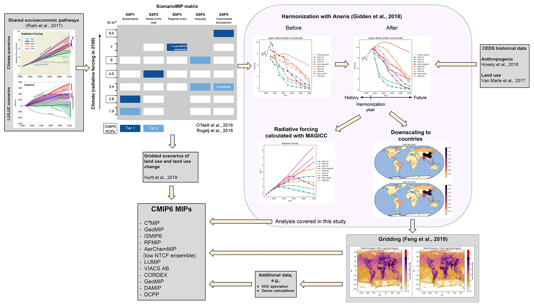
Figure 1The role of ScenarioMIP in the CMIP6 ecosystem. From a population of over 40 possible SSPs, nine are downselected in order to span the climatic and social dimensions of the ScenarioMIP SSP–RCP matrix. Emissions trajectories developed from these scenarios then undergo harmonization to a common and consistent historical dataset, downscaling, and gridding. The resulting emissions datasets are then provided to the CMIP6 scientific community, in conjunction with future scenarios of land use (Hurtt, 2019), concentrations (Meinshausen, 2019), and other domain-specific datasets (e.g., VOC speciation and ozone concentrations).
The remainder of the paper is as follows. First, we discuss scenario selection, historical data aggregation, harmonization, and downscaling methods in Sect. 2. We then present harmonized model results, focusing on overall emissions trajectories, climate response outcomes, and the spatial distribution of key emissions species in Sect. 3. Finally, in Sect. 4, we discuss conclusions drawn from this study as well as guidelines for using the results presented herein in further CMIP6 experiments.
2.1 Socioeconomic and climate scenarios
The global IAM community has developed a family of scenarios that describe a variety of possible socioeconomic futures (the SSPs). The formation, qualitative, and quantitative aspects of these scenarios have been discussed widely in the literature (O'Neill et al., 2017; KC and Lutz, 2017; Dellink et al., 2015; Jiang and O'Neill, 2017). We briefly summarize here relevant narratives of the baseline SSPs concerning socioeconomic development (see, e.g., Fig. A1), energy systems (Bauer et al., 2017), land use (Popp et al., 2017), greenhouse gas (GHG) emissions (Riahi et al., 2017), and air pollution (Rao et al., 2017).
SSP1 and SSP5 describe worlds with strong economic growth via sustainable and fossil fuel pathways, respectively. In both scenarios, incomes increase substantially across the globe and inequality within and between countries is greatly reduced; however, this growth comes at the expense of potentially large impacts from climate change in the case of SSP5. Demand for energy- and resource-intensive agricultural commodities such as ruminant meat is significantly lower in SSP1 due to changes in behavior and advances in energy efficiency. In both scenarios, pollution controls are expanded in high-income economies with other nations catching up relatively quickly with the developed world, resulting in reductions in air pollutant emissions. SSP2 is a so-called middle-of-the-road scenario with moderate population growth and slower convergence of income levels across countries. In SSP2, food consumption, especially for resource-intensive livestock-based commodities, is expected to increase and energy generation continues to rely on fossil fuels at approximately the same rates as today, resulting in continued growth of GHG emissions. Efforts at curbing air pollution continue along current trajectories with developing economies ultimately catching up to high-income nations, resulting in an eventual decrease in pollutant emissions. Finally, SSP3 and SSP4 depict futures with high inequality between countries (i.e., “regional rivalry”) and within countries, respectively. Global gross domestic product (GDP) growth is low in both scenarios and concentrated in currently high-income nations, whereas population increase is focused in low- and middle-income countries. Energy systems in SSP3 see a resurgence of coal dependence, whereas reductions occur in SSP4 as the high-tech energy and economy sectors see increased developments and investments leading to higher diversification of technologies (Bauer et al., 2017). Policy making (either regionally or internally) in areas including land-use regulation, air pollution control, and GHG emissions limits is less effective. Thus policies vary regionally in both SSPs with weak international institutions, resulting in the highest levels of pollutant and aerosol emissions and potential effect on climate outcomes (Shindell et al., 2013).
A matrix of socioeconomic–climate scenarios relevant to the broad scientific community was created with SSPs on one axis and climate policy futures (i.e., mitigation scenarios) delineated by end-of-century (EOC) RF on the other axis (see Fig. 1). The scenarios selected for inclusion in ScenarioMIP, shown in Table 1, are comprised of both baseline and mitigation cases, in which long-term climate policies are lacking or included, respectively. They are divided into Tier-1 scenarios, which span a wide range of uncertainty in future forcing and are utilized by other MIPs, and Tier-2 scenarios, which enable more detailed studies of the effect of mitigation and adaptation policies which fall between the Tier-1 forcing levels. Each scenario is run by a single model within ScenarioMIP, comprised of the AIM/CGE, GCAM4, IMAGE, MESSAGE-GLOBIOM, and REMIND-MAgPIE modeling teams. We provide a short discussion here on their selection and refer the reader to O'Neill et al. (2016, Sect. 3.2.2) for fuller discussion of the experimental design.
The Tier-1 scenarios include SSP1-2.6, SSP2-4.5, SSP3-7.0, and SSP5-8.5, designed to provide a full range of forcing targets similar in both magnitude and distribution to the RCPs as used in CMIP5. Each EOC forcing level is paired with a specific SSP, which is chosen based on the relevant experimental coverage. For example, SSP2 is chosen for the 4.5 W m−2 experiment because of its high relevance as a reference scenario to IAV communities as a scenario with intermediate vulnerability and climate forcing and its median positioning of land use and aerosol emissions (of high importance for DAMIP and DCPP), whereas SSP3 is chosen for the 7.0 W m−2 experiment as it allows for quantification of avoided impacts (e.g., relative to SSP2) and has significant emissions from near-term climate forcing (NTCF) species such as aerosols and methane (also referred to as short-lived climate forcers, or SLCF).
The Tier-2 scenarios include SSP1-1.9, SSP3-LowNTCF, SSP4-3.4, SSP4-6.0, and SSP5-3.4-Overshoot (OS), chosen to both complement and extend the types of scenarios available to climate modelers beyond those analyzed in CMIP5. SSP1-1.9 provides the lowest estimate of future forcing matching the most ambitious goals of the Paris Agreement (i.e., “pursuing efforts to limit the [global average] temperature increase to 1.5 ∘C above pre-industrial levels”). The SSP3-LowNTCF scenario provides an important experimental comparison to scenarios with high NTCFs for use in AerChemMIP (Collins et al., 2017) contrasting with SSP3-7.0 (see Appendix Appendix C for more detail on differences in assumptions between SSP3-7.0 and SSP3-LowNTCF). Both SSP4 scenarios fill gaps in Tier-1 forcing pathways and allow investigations of impacts in scenarios with relatively strong land-use and aerosol climate effects but relatively low challenges to mitigation. Finally, SSP5-3.4-OS allows for the study of a scenario in which there is large overshoot in RF by mid-century followed by the implementation of substantive policy tools to limit warming in the latter half of the century. It is specifically designed to be twinned with SSP5-8.5, following the same pathway through 2040, and support experiments examining delayed climate action.
Table 1All scenarios and associated attributes used in the ScenarioMIP experiment ensemble.

2.2 Historical emissions data
We construct a common dataset of historical emissions for the year 20151, the transition year in CMIP6 between historic and future model runs, using two primary sources developed for CMIP6. Hoesly et al. (2018) provide data over 1750–2014 for anthropogenic emissions by country. They include a detailed sectoral representation (59 sectors in total) which has been aggregated into nine individual sectors (see Appendix Table ), including agriculture, aircraft, energy, industry, international shipping, residential and commercial, solvent production and application, transportation, and waste. Values for 2015 were approximated by extending fossil fuel consumption using aggregate energy statistics (BP, 2016) and trends in emissions factors from the GAINS ECLIPSE V5a inventory (Klimont et al., 2017; Stohl et al., 2015). Sulfur (SOx) emissions in China were trended from 2010 using values from Zheng et al. (2018).
The study of van Marle et al. (2017) provides data on historical emissions from open burning, specifically including burning of agricultural waste on fields (AWB), forests, grasslands, and peatlands out to 2015. Due to the high amount of inter-annual variability in the historical data which is not explicitly modeled in IAMs, we use a decadal mean over 2005–2014 to construct a representative value for 2015 (see, e.g., Fig. A2). When used in conjunction with model results, we aggregate country-level emissions to the individual model regions of which they are comprised.
Emissions of N2O and fluorinated gas species were harmonized only at the global level, with 2015 values from other data sources. Global N2O emissions were taken from PRIMAP (Gütschow et al., 2016) and global emissions of HFCs were developed by Velders et al. (2015). The HFC-23 and total PFC and SF6 emissions were provided by Guus Velders, based on Carpenter et al. (2014) mixing ratios, and were extended from 2012 to 2015 by using the average 2008–2012 trend.
2.3 Automated emissions harmonization
Emissions harmonization is defined as a procedure designed to match model results to a common set of historical emissions trajectories. The goal of this process is to match a specified base-year dataset while retaining consistency with the original model results to the best extent possible while also providing a smooth transition from historical trajectories. This non-disjoint transition is critical for global climate models when modeling projections of climate futures which depend on historical model runs, guaranteeing a smooth functional shape of both emissions and concentration fields between the historical and future runs. Models differ in their 2015 data points in part because the historical emissions datasets used to calibrate the models differ (e.g., PRIMAP – Gütschow et al., 2016; EDGAR – Crippa et al., 2016; CEDS – Hoesly et al., 2018). Another cause of differences is that 2015 is a projection year for all of these models (the original scenarios were originally finalized in 2015).
Harmonization can be simple in cases where a model's historical data are similar to the harmonization dataset. However, when there are strong discrepancies between the two datasets, the choice of harmonization method is crucial for balancing the dual goals of accurate representation of model results and reasonable transitions from historical data to harmonized trajectories.
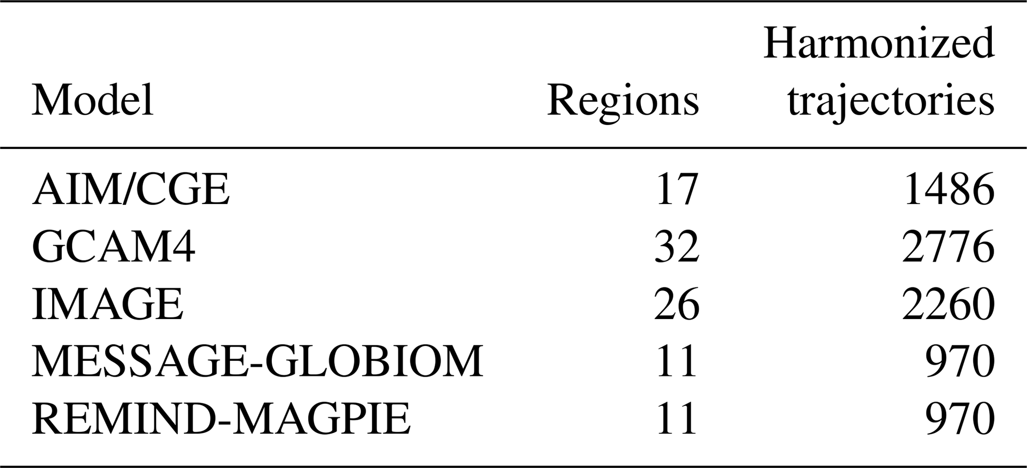
The quantity of trajectories requiring harmonization increases the complexity of the exercise. In this analysis, given the available sectoral representation of both the historical data and models, we harmonize model results for 14 individual emissions species and 13 sectors as described in Table 2. The majority of emissions–sector combinations are harmonized for every native model region2 (Table 3). Global trajectories are harmonized for fluorinated species and N2O, aircraft and international shipping sectors, and CO2 agriculture, forestry, and other land-use (AFOLU) emissions due to historical data availability and regional detail. Therefore between 970 and 2776 emissions trajectories require harmonization for any given scenario depending on the model used.
Table 2Harmonized species and sectors, adapted from Gidden et al. (2018) with permission of the authors. A mapping of original model variables (i.e., outputs) to ScenarioMIP sectors is shown in Appendix Table B2.
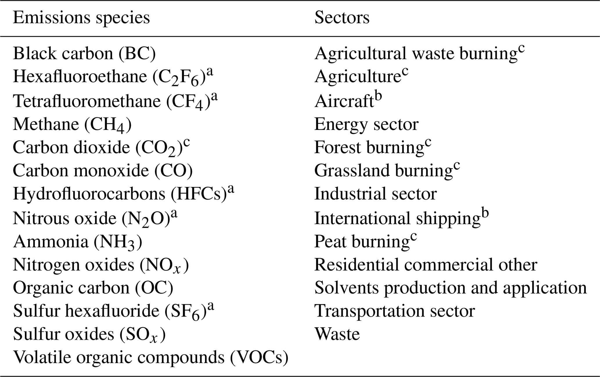
a Global total trajectories are harmonized due to lack of detailed historical data. b Global sectoral trajectories are harmonized due to lack of detailed historical data. c A global trajectory for AFOLU CO2 is used; non-land-use sectors are harmonized for each model region.
Table 3The number of model regions and total harmonized emissions trajectories for each IAM participating in the study. The number of trajectories is calculated from Table 2, including gas species for which global trajectories are harmonized.
We employ the newly available open-source software Aneris (Gidden et al., 2018; Gidden, 2017) in order to perform harmonization in a consistent and rigorous manner. For each trajectory to be harmonized, Aneris chooses which harmonization method to use by analyzing both the relative difference between model results and harmonization historical data as well as the behavior of the modeled emissions trajectory. Available methods include ratio and offset methods, which utilize the quotient and difference of unharmonized and harmonized values, respectively, as well as convergence methods, which converge to the original modeled results at some future time period. We refer the reader to Gidden et al. (2018) for a full description of the harmonization methodology and implementation.
Override methods can be specified for any combination of species, sectors, and regions which are used in place of the default methods provided by Aneris. Override methods are useful when default methods do not fully capture either the regional or sectoral context of a given trajectory. Most commonly, we observed this in cases where there are large relative differences in the historical datasets, the base-year values are small, and there is substantial growth in the trajectory over the modeled time period, thereby reflecting the large relative difference in the harmonized emissions results. However, the number of required override methods is small: 5.1 % of trajectories use override messages for the IMAGE model, 5.6 % for MESSAGE-GLOBIOM, and 9.8 % for REMIND. The AIM model elected not to use override methods, and GCAM uses a relatively large number (35 %).
Finally, in order to provide additional detail for fluorinated gases (F gases) we extend the set of reported HFC and CFC species based on exogenous scenarios. We take scenarios of future HFCs from Velders et al. (2015), which provide detailed emissions trajectories for F gases. We downscale the global HFC emissions reported in each harmonized scenario to arrive at harmonized emissions trajectories for all constituent F gases, deriving the HFC-23 from the RCP emissions pathway. We further include trajectories of CFCs as reported in scenarios developed by the World Meteorological Organization (WMO) (Carpenter et al., 2014), which are not included in all model results.
2.4 Region-to-country downscaling
Downscaling, defined here as distributing aggregated regional values to individual countries, is performed for all scenarios in order to improve the spatial resolution of emissions trajectories, and as a prelude to mapping to a spatial grid (discussed in Appendix Appendix D). We developed an automated downscaling routine that differentiates between two classes of sectoral emissions: those related to AFOLU and those related to fuel combustion and industrial and urban processes. In order to preserve as much of the original model detail as possible, the downscaling procedures here begin with harmonized emissions data at the level of native model regions and the aggregate sectors (Table 2). Here we discuss key aspects of the downscaling methodology and refer the reader to the downscaling documentation (https://github.com/iiasa/emissions_downscaling/wiki, last access: 8 April 2019) for further details.
AFOLU emissions, including agricultural waste burning, agriculture, forest burning, peat burning, and grassland burning, are downscaled using a linear method. Linear downscaling means that the fraction of regional emissions in each country stays constant over time. Therefore, the total amount of open-burning emissions allocated to each country will vary over time as economies evolve into the future, following regional trends from the native IAM. However there is no subregional change in the spatial distribution of land-use related emissions over time. This is in contrast to other anthropogenic emissions, where the impact, population, affluence, and technology (IPAT) method is used to dynamically downscale to the country level as discussed above. Note that peat burning emissions were not modeled by the IAMs and are constant into the future.
All other emissions are downscaled using the IPAT (Ehrlich and Holdren, 1971) method developed by van Vuuren et al. (2007), where population and GDP trajectories are taken from the SSP scenario specifications (KC and Lutz, 2017; Dellink et al., 2015). The overall philosophy behind this method is to assume that emissions intensity values (i.e., the ratio of emissions to GDP) for countries within a region will converge from a base year, ti (2015 in this study), over the future. A convergence year, tf, is specified beyond 2100, the last year for the downscaled data, meaning that emissions intensities do not converge fully by 2100. The choice of convergence year reflects the rate at which economic and energy systems converge toward similar structures within each native model region. Accordingly, the SSP1 and SSP5 scenarios are assigned relatively near-term convergence years of 2125, while SSP3 and SSP4 scenarios are assigned 2200, and SSP2 is assigned an intermediate value of 2150.
The downscaling method first calculates an emissions intensity, I, for the base and convergence years using emissions level, E, and GDP.
An emissions intensity growth factor, β, is then determined for each country, “c”, within a model region, “R”, using convergence year emissions intensities, , determined by extrapolating from the last 10 years (e.g., 2090 to 2100) of the scenario data.
Using base-year data for each country and scenario data for each region, future downscaled emissions intensities and patterns of emissions are then generated for each subsequent time period.
These spatial patterns are then scaled with (i.e., normalized to) the model region data to guarantee consistency between the spatial resolutions, resulting in downscaled emissions for each country in each time period.
For certain countries and sectors the historical dataset has zero-valued emissions in the harmonization year. This would result in zero downscaled future emissions for all years. Zero emissions data occur largely for small countries, many of them small island nations. This could be due to either lack of actual activity in the base year or missing data on activity in those countries. In order to allow for future sectoral growth in such cases, we adopt, for purposes of the above calculations, an initial emissions intensity of one-third the value of the lowest country in the same model region. We then allocate future emissions in the same manner discussed above, which is consistent with our overall convergence assumptions. Note that we exclude the industrial sector (Table 2) from this operation as it might not be reasonable to assume the development of substantial industrial activity in these countries.
Finally, some scenarios include negative CO2 emissions at some point in the future (notably from energy use). For CO2 emissions, therefore, we apply a linear rather than exponential function to allow a smooth transition to negative emissions values for both the emissions intensity growth factor and future emissions intensity calculations. In such cases, Eqs. (2) and (3) are replaced by Eqs. (6) and (7), respectively.
Here we present the results of harmonization and downscaling applied to all nine scenarios under consideration. We discuss in Sect. 3.1 the relevance of each selected scenario to the overall experimental design of ScenarioMIP, focusing on their RF and mean global temperature pathways. In Sect. 3.2, we discuss general trends in global trajectories of important GHGs and aerosols and their sectoral contributions over the modeled time horizon. In Sect. 3.3, we explore the effect of harmonization on model results and the difference between unharmonized and harmonized results. Finally, in Sect. 3.4, we provide an overview of the spatial distribution of emissions species at both regional and spatial grids.
3.1 Experimental design and global climate response
The nine ScenarioMIP scenarios were selected to provide a robust experimental design space for future climate studies as well as IAV analyses with the broader context of CMIP6. Chief among the concerns in developing such a design space are both the range and spacing of the global climate response within the portfolio of scenarios (Moss et al., 2008). Prior work for the RCPs studied a range of climate outcomes between ∼2.6 and 8.5 W m−2 at EOC. Furthermore, recent work (Tebaldi et al., 2015) finds that statistically significant regional temperature outcomes (>5 % of half the land surface area) are observable with a minimum separation of 0.3 ∘C, which is approximately equivalent to 0.75 W m−2 (O'Neill et al., 2016). Given the current policy context, notably the recent adoption of the UN Paris Agreement, the primary design goal for the ScenarioMIP scenario selection is thus twofold: span a wider range of possible climate futures (1.9–8.5 W m−2) in order to increase relevance to the global climate dialogue and provide a variety of scenarios between these upper and lower bounds such that they represent statistically significant climate variations in order to support a wide variety of CMIP6 analyses.
We find that the selected scenarios meet this broad goal, as shown in Fig. 2, by using the simple climate model MAGICC6 with central climate-system and gas-cycle parameter settings for all scenarios to calculate pathways of both RF and the resulting response of global mean temperature (see Appendix Table B3 for a listing of all EOC RF values).
We also present illustrative global mean temperature pathways. EOC temperature outcomes span a large range, from 1.4 ∘C at the lower end to 4.9 ∘C for SSP5-8.5, the scenario with the highest warming emissions trajectories. Notably, two scenarios (SSP1-1.9, which reaches 1.4 ∘C by EOC, and SSP1-2.6, reaching 1.7 ∘C) can be used for studies of global outcomes of the implementation of the UN Paris Agreement, which has a desired goal of “[h]olding the increase in the global average temperature to well below 2 ∘C above pre-industrial levels and pursuing efforts to limit the temperature increase to 1.5 ∘C above pre-industrial levels” (United Nations, 2016, Article 2.1(a)). The difference between scenario temperature outcomes is statistically significant in nearly all cases, with a minimum difference of 0.37 ∘C (SSP1-1.9 and SSP1-2.6) and maximum value of 0.77 ∘C (SSP3-7.0 and SSP5-8.5). The EOC difference between SSP4-3.4 and SSP5-3.4-OS is not significant (0.07 ∘C); however global climate outcomes are likely sensitive to the dynamics of the forcing pathway (Tebaldi et al., 2015).
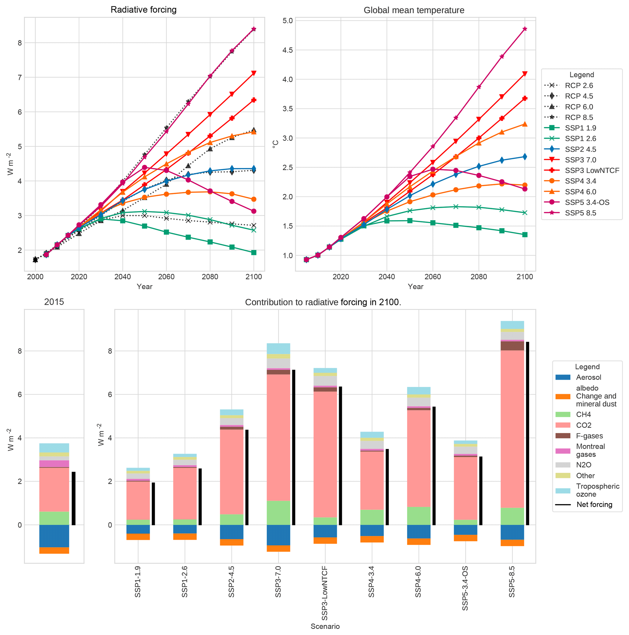
Figure 2Trajectories of RF and global mean temperature (above pre-industrial levels) are presented as are the contributions to RF for a number of different emissions types native to the MAGICC6 model. The RF trajectories are displayed with their RCP counterparts analyzed in CMIP5. For those scenarios with direct analogues, trajectories are largely similar in shape and match the same EOC forcing values.
A subset of four scenarios (SSP1-2.6, SSP2-4.5, SSP4-6.0, and SSP5-8.5) was also designed to provide continuity between CMIP5 and CMIP6 by providing similar forcing pathways to their RCP counterparts assessed in CMIP5. We find that this aspect of the scenario design space is also met by the relevant scenarios. SSP2-4.5 and SSP5-8.5 track RCP4.5 and RCP8.5 pathways nearly exactly. We observe slight deviations between SSP1-2.6 and RCP2.6 as well as SSP4-6.0 and RCP6.0 at mid-century due largely to increased methane emissions in the historic period (i.e., methane emissions broadly follow RCP8.5 trajectories after 2000, resulting in higher emissions in the harmonization year of this exercise; see Fig. 3 below).
The remaining five scenarios were chosen to “fill gaps” in the previous RCP studies in CMIP5 and enhance the potential policy relevance of CMIP6 MIP outputs (O'Neill et al., 2016). SSP3-7.0 was chosen to provide a scenario with relatively high vulnerability and land-use change with associated near-term climate forcing (NTCF) emissions resulting in a high RF pathway. We find that it reaches an EOC forcing target of ∼7.1 W m−2 and greater than 4 ∘C mean global temperature increase. While contributions to RF from CO2 in SSP3-7.0 are lower than that of SSP5-8.5, methane and aerosol contributions are considerably higher (see, e.g., Etminan et al., 2016, for a discussion on the effect of shortwave forcing on methane's contribution to overall RF). A companion scenario, SSP3-LowNTCF, was also included in order to study the effect of NTCF species in the context of AerChemMIP. Critically, emissions factors of key NTCF species are assumed to develop similar to an SSP1 (rather than SSP3) scenario. SSP3-LowNTCF sees substantially fewer contributions to EOC forcing from NTCF emissions (notably SOx and methane), resulting in a forcing level of 6.3 W m−2 and global mean temperature increase of 3.75 ∘C by the end of the century. This significant reduction is largely due to updating emissions coefficients for air pollutants and other NTCFs to match the SSP1 assumptions. SSP4-3.4 was chosen to provide a scenario at the lower end of the range of future forcing pathways. Reaching a EOC mean global temperature between SSP2-4.5 and SSP1-2.6 (∼2.25 ∘C), it is an ideal scenario for scientists to study the mitigation costs and associated impacts between forcing levels of 4.5 and 2.6 W m−2.
The final two scenarios, SSP1-1.9 and SSP5-3.4-OS, were chosen to study policy-relevant questions of near- and medium-term action on climate change. SSP1-1.9 provides a new low end to the RF pathway range. It reaches an EOC forcing level of ∼1.9 W m−2 and an associated global mean temperature increase of ∼1.4 ∘C (with temperature peaking in 2040), in line with the goals of the Paris Agreement. SSP5-3.4-OS, however, is designed to represent a world in which action towards climate change mitigation is delayed but vigorously pursued after 2050, resulting in a forcing and mean global temperature overshoot. A peak temperature of 2.5 ∘C above pre-industrial levels is reached in 2060 after which global mitigation efforts reduce EOC warming to ∼2.25 ∘C. In tandem, and including SSP2-4.5 (which serves as a reference experiment in ScenarioMIP; O'Neill et al., 2016), these scenarios provide a robust experimental platform to study the effect of the timing and magnitude of global mitigation efforts, which can be especially relevant to science-informed policy discussions.
3.2 Global emissions trajectories
Emissions contributions to the global climate system are myriad but can broadly be divided into contributions from greenhouse gases (GHGs) and aerosols. The models used in this analysis explicitly represent manifold drivers and processes involved in the emissions of various gas species. For a fuller description of these scenario results see the original SSP quantification papers (van Vuuren et al., 2017; Fricko et al., 2017; Fujimori et al., 2017; Calvin et al., 2017; Kriegler et al., 2017). Here, we focus on emissions species that most strongly contribute to changes in future mean global temperature and scenarios with the highest relevance and uptake for other MIPs within CMIP6, namely the Tier-1 scenarios SSP1-2.6, SSP2-4.5, SSP3-7.0, and SSP5-8.5. Where insightful, we provide additional detail on results from other scenarios; however results for all scenarios are available in Appendix Appendix E.
CO2 emissions have a large span across scenarios by the end of the century (−20 to 125 Gt yr−1), as shown in Fig. 3. Scenarios can be categorized based on characteristics of their trajectory profiles: those that have consistent downward trajectories (SSP1, SSP4-3.4), those that peak in a given year and then decrease in magnitude (SSP2-4.5 in 2040 and SSP4-6.0 in 2050), and those that have consistent growth in emissions (SSP3). SSP5 scenarios, which model a world with fossil-fuel-driven development, have EOC emissions which bound the entire scenario set, with the highest CO2 emissions in SSP5-8.5 peaking in 2080 and the lowest CO2 emissions in SSP5-3.4-OS resulting from the application of stringent mitigation policies after 2040 in an attempt to stabilize RF to 3.4 W m−2 after overshooting this limit earlier in the century. A number of scenarios exhibit negative net CO2 emissions before the end of the century. SSP1-1.9, the scenario with the most consistent negative emissions trajectory, first reports net negative emissions in 2060 with EOC emissions of −14 Gt yr−1. SSP5-3.4-OS, SSP1-2.6, and SSP4-3.4 each cross the zero-emissions threshold in 2070, 2080, and 2090, respectively.
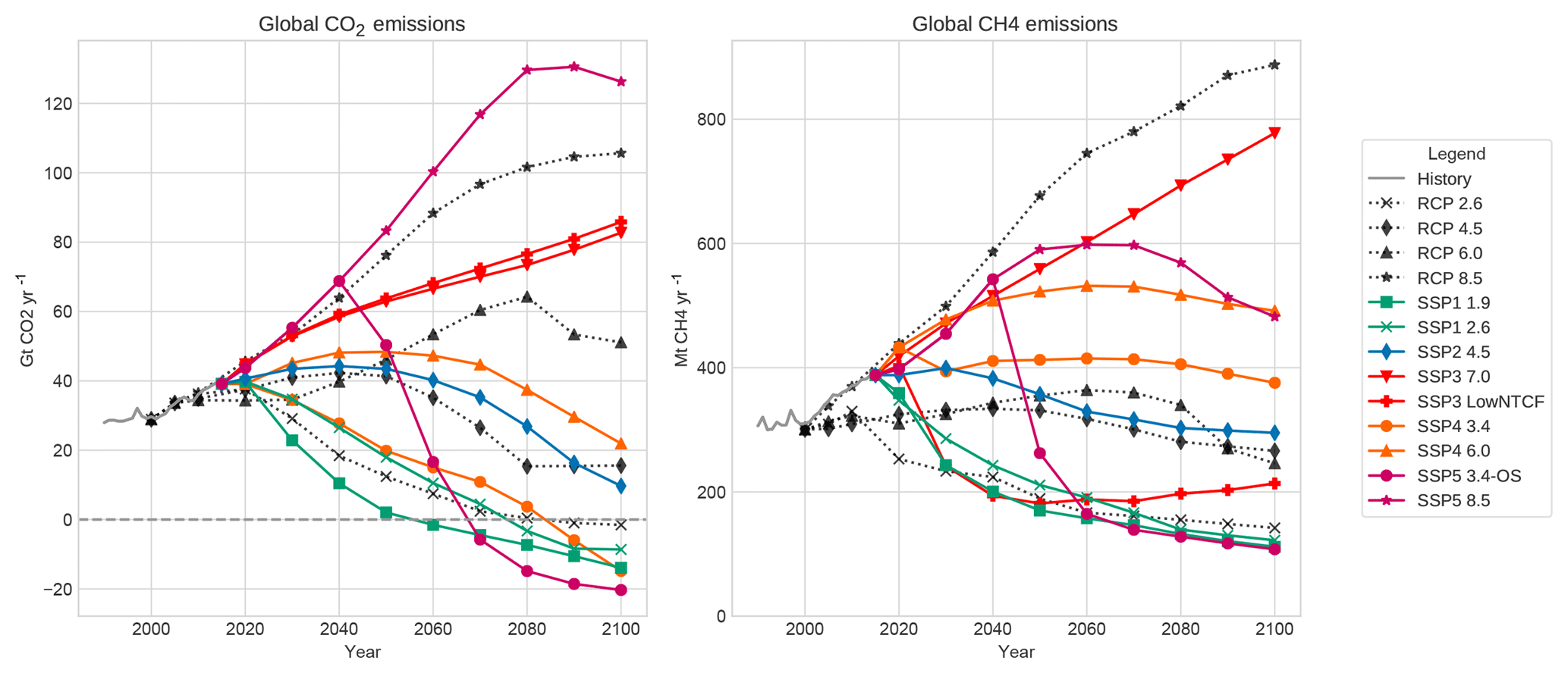
Figure 3Trajectories of CO2 and CH4, primary contributors to GHG emissions, including both historical emissions, emissions analyzed for the RCPs, and all nine scenarios covered in this study.
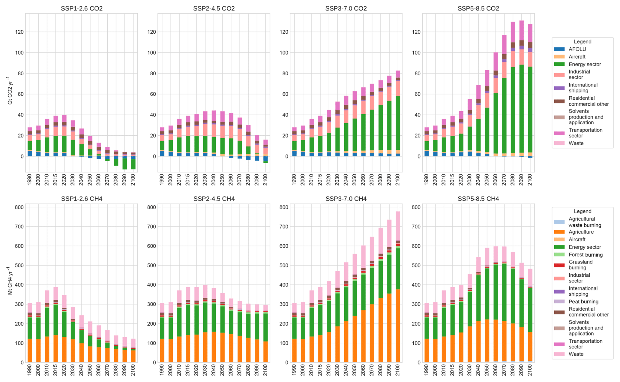
Global emissions trajectories for CO2 are driven largely by the behavior of the energy sector in each scenario, as shown in Fig. 4. Positive emissions profiles are also greatly influenced by the industry and transport sectors, whereas negative emissions profiles are driven by patterns of agriculture and land-use as well as the means of energy production. In SSP1-2.6, early to mid-century emissions continue to be dominated by the energy sector with substantial contributions from industry and transport. Negative emissions from land use are observed as early as 2030 due to large-scale afforestation (Popp et al., 2017; van Vuuren et al., 2017) while net negative emissions from energy conversion first occur in 2070. Such net negative emissions are achieved when carbon dioxide removal from bioenergy from carbon capture and storage (CCS) exceeds residual fossil CO2 emissions from the combustion of coal, oil, and gas. Emissions contributions from the transport sector diminish over the century as heavy- and light-duty transport fleets are electrified. Emissions from industry peak and the decrease over time such that the residential and commercial sector (RC) provides the majority of positive CO2 emissions by the end of the century. SSP2-4.5 experiences similar trends among sectors but with smaller magnitudinal changes and temporal delays. Negative emissions, for example, are experienced in the land-use sector for the first time in 2060 and are not experienced in the energy sector until the end of the century. Energy-sector CO2 emissions continue to play a large role in the overall composition until 2080, at which point the industrial sector provides the plurality of CO2. Emissions from the transport sector peak at mid-century, but are still a substantive component of positive CO2 emissions at the end of the century. Finally, the SSP5-8.5 scenario's emissions profile is dominated by the fossil-fueled energy sector for the entirety of the century. Contributions from the transport and industrial sectors grow in magnitude but are diminished as the share of total CO2 emissions, CO2 emissions from the AFOLU sector, decrease steadily over time. By the end of the century, the energy sector comprises almost 75 % of all emitted CO2 in this scenario relative to 50 % today.
Methane (CH4) is an emissions species with substantial contributions to potential future warming mainly due to its immediate GHG effect, but also because of its influence on atmospheric chemistry, as a tropospheric ozone precursor, and its eventual oxidation into CO2 in the case of CH4 from fossil sources (Boucher et al., 2009). At present, approximately 400 Mt yr−1 of CH4 is emitted globally, and the span of future emissions developed in this scenario set range from 100 to nearly 800 Mt yr−1 by the end of the century. Global emissions of methane in SSP1 scenarios follow similar trajectories to CO2, with large emissions reductions; SSP2 follows suit, with emissions peaking in 2030 and then reducing throughout the rest of the century; in SSP3's baseline scenario, emissions continue to grow while in the NTCF scenario they are reduced drastically as policies are implemented to reduce forcing from short-lived emissions species; SSP4 is characterized by growing (SSP4-6.0) or mostly stable (SSP4-3.4) CH4 emissions until the middle of the century which peak in 2060 and then decline; and finally SSP5's baseline scenario sees a plateauing of CH4 emissions between 2050 and 2070 before their eventual decline, while the overshoot scenario has drastic CH4 emissions reductions in 2040 corresponding to significant mid-century mitigation efforts in that scenario.
Historically, CH4 emissions are dominated by three sectors: energy (due to fossil fuel production and natural gas transmission), agriculture (largely enteric fermentation from livestock and rice production), and waste (i.e., landfills). In each scenario, global emissions of CH4 are largely dominated by the behavior of activity in each of these sectors over time. For example, in the SSP1 scenarios, significant reductions in energy emissions are observed as energy supply systems shift from fossil to renewable sources while agriculture and waste-sector emissions see only modest reductions as global population stabilizes around mid-century. In the SSP2 scenario, emissions from the energy sector peak in 2040 as there is continued reliance on energy from natural gas but large expansions in renewables in the future; however, emissions from the agricultural and waste sectors are similar to today's levels by the end of the century. Finally, CH4 emissions in SSP5's baseline scenario are characterized by growth in the energy sector from continued expansion of natural gas and a peak and reduction in agricultural emissions resulting in 20 % higher emissions at the end of the century relative to the present as population grows in the near term before contracting globally.
GHG emissions are broadly similar between the main scenarios in CMIP5 (RCPs) and CMIP6 (SSPs). Notably, we observe that the SSPs exhibit slightly lower CO2 emissions in the 2.6 W m−2 scenarios and higher emissions in the 8.5 W m−2 scenarios due to lower and higher dependence on fossil fuels relative to their RCP predecessors. CH4 emissions are largely similar at EOC for 2.6 and 4.5 W m−2 scenarios between the RCPs and SSPs, with earlier values differing due to continued growth in the historical period (RCPs begin in 2000 whereas SSPs begin in 2015). The 8.5 W m−2 scenario exhibits the largest difference in CH4 emissions between the RCPs and SSPs because of the SSP5 socioeconomic story line depicting a world which largely develops out of poverty in less-developed countries, reducing CH4 emissions from waste and agriculture. This contrasts with a very different story line behind RCP8.5 (Riahi et al., 2011).
In nearly all scenarios, aerosol emissions are observed to decline over the century; however, the magnitude and speed of this decline are highly dependent on the evolution of various drivers based on the underlying SSP story lines, resulting in a wide range of aerosol emissions, as shown in Fig. 5. For example, sulfur emissions (totaling 112 Mt yr−1 globally in 2015) are dominated at present by the energy and industrial sectors. In SSP1, where the world transitions away from fossil-fuel-related energy production (namely coal in the case of sulfur), emissions decline sharply as the energy sector transitions to non-fossil-based fuels and end-of-pipe measures for air pollution control are ramped up swiftly. The residual amount of sulfur remaining at the end of the century (∼10 Mt yr−1) is dominated by the industrial sector. SSP2-4.5 sees a similar transition but with delayed action: total sulfur emissions decline due primarily to the decarbonization of the energy sector. SSP5 also observes declines in overall sulfur emissions led largely by an energy mix that transitions from coal dependence to dependence on natural gas, as well as strong end-of-pipe air pollution control efforts. These reductions are similarly matched in the industrial sector, where natural gas is substituted for coal use as well. Thus, overall reductions in emissions are realized across the scenario set. Only SSP3 shows EOC sulfur emissions equivalent to the present day, largely due to increased demand for industrial services from growing population centers in developing nations with a heavy reliance on coal-based energy production and weak air pollution control efforts.
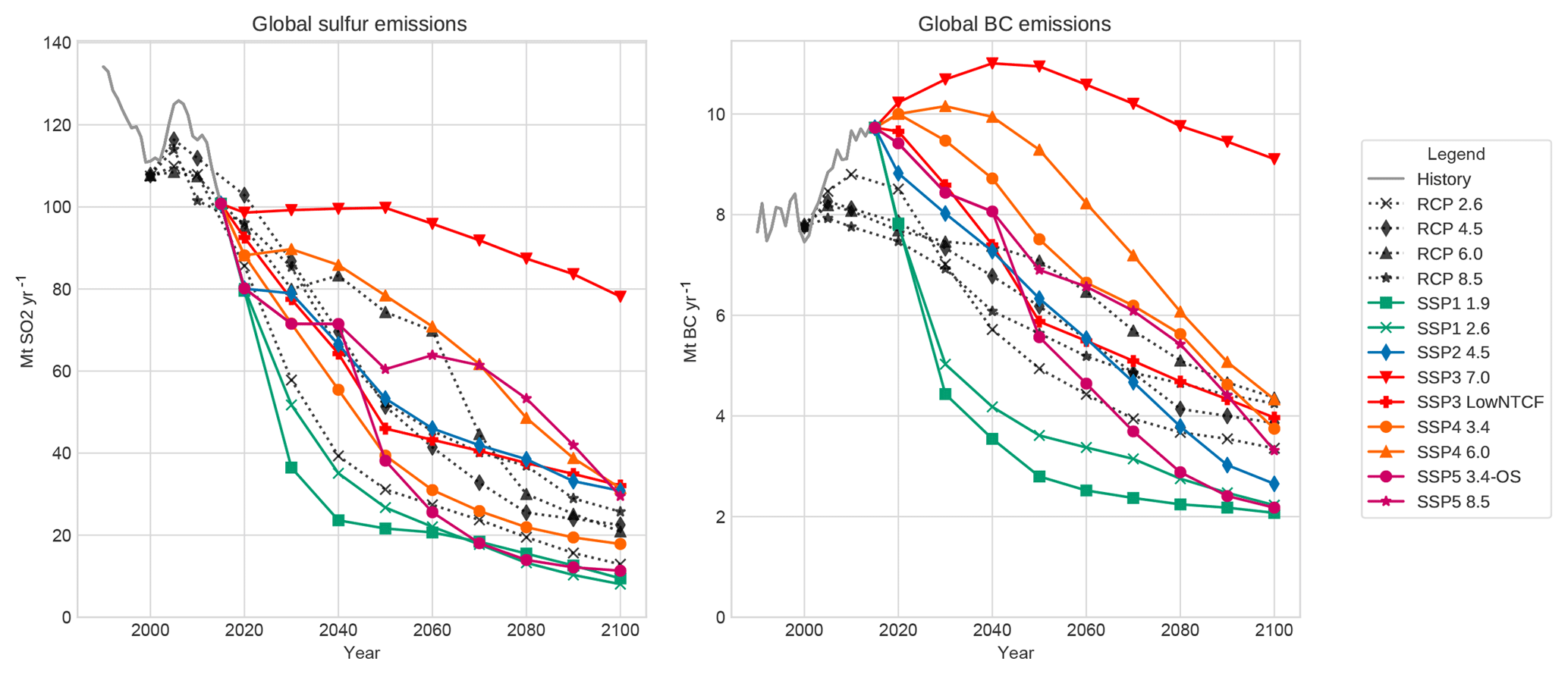
Figure 5Emissions trajectories for sulfur and black carbon (BC), for history, the RCPs, and all nine scenarios analyzed in this study. SSP trajectories largely track with RCP values studied in CMIP5. A notable difference lies in BC emissions, which have seen relatively large increases in past years, thus providing higher initial emissions for the SSPs.
Aerosols associated with the burning of traditional biomass, crop, and pasture residues, as well as municipal waste, such as black carbon (BC) and organic carbon (OC, see Appendix Fig. E3), are affected most strongly by the degree of economic progress and growth in each scenario, as shown in Fig. 6. For example, BC emissions from the residential and commercial sector comprise nearly 40 % of all emissions in the historical time period with a significant contribution from mobile sources. By the end of the century, however, emissions associated with crop and pasture activity comprise the plurality of total emissions in SSP1, SSP2, and SSP5 due to a transition away from traditional biomass usage based on increased economic development and population stabilization and emissions controls on mobile sources. Only SSP3, in which there is continued global inequality and the persistence of poor and vulnerable urban and rural populations, are there continued quantities of BC emissions across sectors similar to today. OC emissions are largely from biofuel and open burning and follow similar trends: large reductions in scenarios with higher income growth rates with a residual emissions profile due largely to open-burning-related emissions. Other pollutant emissions (e.g., NOx, carbon monoxide, CO; and volatile organic carbon, VOC) also see a decline in total global emissions at rates depending on the story line (Rao et al., 2017).
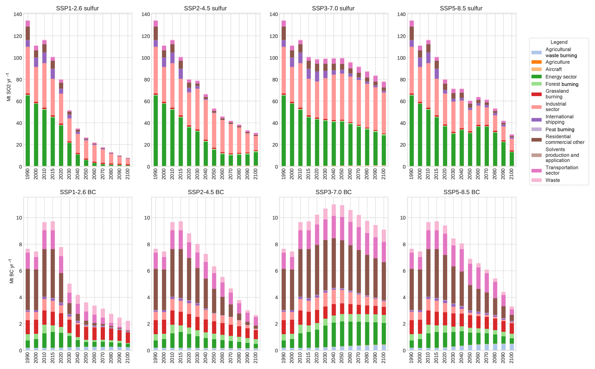
Figure 6The sectoral contributions to sulfur and black carbon emissions for Tier-1 scenarios.
3.3 The effects of harmonization
Harmonization, by definition, modifies the original model results such that base-year values correspond to an agreed-upon historical source, with an aim for future values to match the original model behavior as much as possible. Model results are harmonized separately for each individual combination of model region, sector, and emissions species. In the majority of cases, model results are harmonized using the default methods described in Sect. 2.3; however, it is possible for models to provide harmonization overrides in order to explicitly set a harmonization method for a given trajectory.
We assess the impact that harmonization has on model results by analyzing the harmonized and unharmonized trajectories. Figure 7 shows global trajectories for each scenario of a selected number of emissions species. Qualitatively, the CO2 and sulfur emissions trajectories match relatively closely to the magnitude of model results due to general agreement between historical sources used by individual models and the updated historical emissions datasets. This leads to convergence harmonization routines being used by default. In the case of CH4 and BC, however, there is larger disagreement between model results and harmonized results in the base year. In such cases, Aneris chooses harmonization methods that match the shape of a given trajectory rather than its magnitude in order to preserve the relationship between driver and emissions for each model.
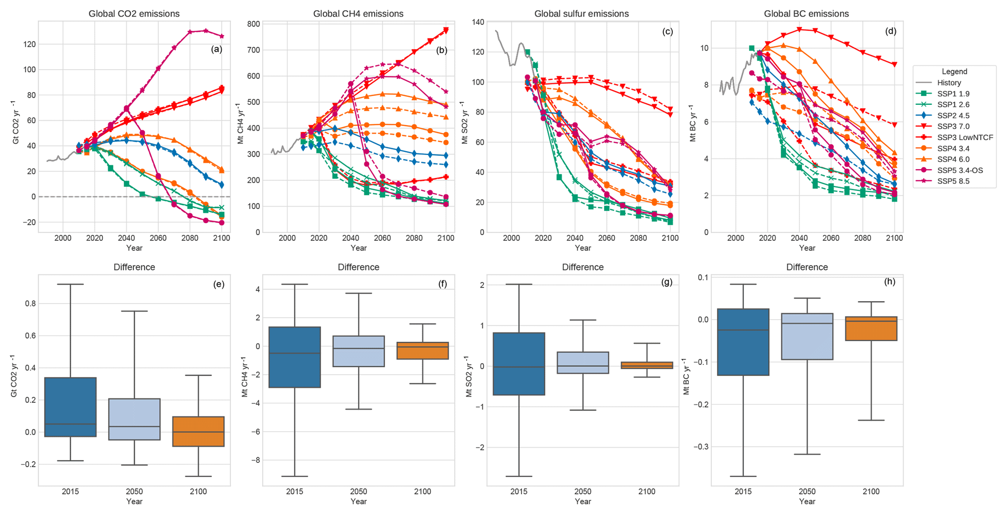
Figure 7Harmonized (solid) and unharmonized (dashed) trajectories are shown are shown in Panels (a)–(d). Panels (e)–(h) depict the distribution of differences (harmonized and less unharmonized) for every modeled region. All box plots show upper and lower quartiles as solid boxes, median values as solid lines, and whiskers extending to the 10th and 90th percentiles. Median values for all are near zero; however, the deviation decreases with time as harmonized values begin to more closely match unharmonized model results largely due to the use of convergence methods.
We find that across all harmonized trajectories the difference between harmonized and unharmonized model results decreases over the modeled time horizon. Panels (e–h) in Fig. 7 show the distribution of all 15 954 trajectories (unharmonized and less harmonized result) for the harmonization year (2015) and two modeled years (2050 and 2100). Each emissions species data population exhibits the same trend of reduced difference between modeled and harmonized results. Not only does the deviation of result distributions decrease over time, but the median value also converges toward zero in all cases.
The trajectory behavior for a number of important emissions species is dominated by certain sectors, as shown in Appendix Fig. F1. Notably, the energy sector tends to dominate behavior of CO2 emissions, agriculture dominates CH4 emissions trajectories, the industrial sector largely determines total sulfur emissions, and emissions from the residential and commercial sectors tend to dominate BC emissions across the various scenarios. Accordingly, we further analyzed the harmonization behavior of these sector–species combinations. Importantly, we again observe an overall trend towards convergence of results at the end of the century; thus harmonized results largely track unharmonized results for these critical emissions sectors. The deviation of distributions of differences consistently decreases with time for all scenarios, and nearly all medians converge consistently towards zero, save for energy-related CO2 SSP5-8.5, which has a higher growth rate than convergence rate, thus larger differences in 2050 than 2015. Overall, we find the harmonization procedure successfully harmonized results' historical base year and closely matches model results across the scenarios by EOC.
3.4 Spatial distribution of emissions
The extent to which reductions or growth of emissions are distributed regionally varies greatly among scenarios. The regional breakdown of primary contributors to future warming potential, CO2 and CH4, is shown in Fig. 8. While present-day CO2 emissions see near-equal contributions from the Organization for Economic Cooperation and Development (OECD) and Asia, future CO2 emissions are governed largely by potential developments in Asia (namely China and India). For SSP1-2.6, in which deep decarbonization and negative CO2 emissions occur before the end of the century, emissions in Asia peak in 2020 before reducing to zero by 2080. Mitigation efforts occur across all regions, and the majority of carbon reduction is focused in the OECD; however, all regions have net negative CO2 emissions by 2090. Asian CO2 emissions in SSP2-4.5 peak in 2030, and most other regions see overall reductions except Africa, in which continued development and industrialization results in emissions growth. Notably, Latin America is the only region in which negative emissions occur in SSP2-4.5 due largely to increased deployment of biomass-based energy production and carbon sequestration. Sustained growth across regions is observed in SSP5-8.5, where emissions in Asia peak by 2080, driving the global emissions peaking in the same year. Other scenarios (see Appendix Fig. G1) follow similar trends with future CO2 emissions driven primarily by developments in Asia.
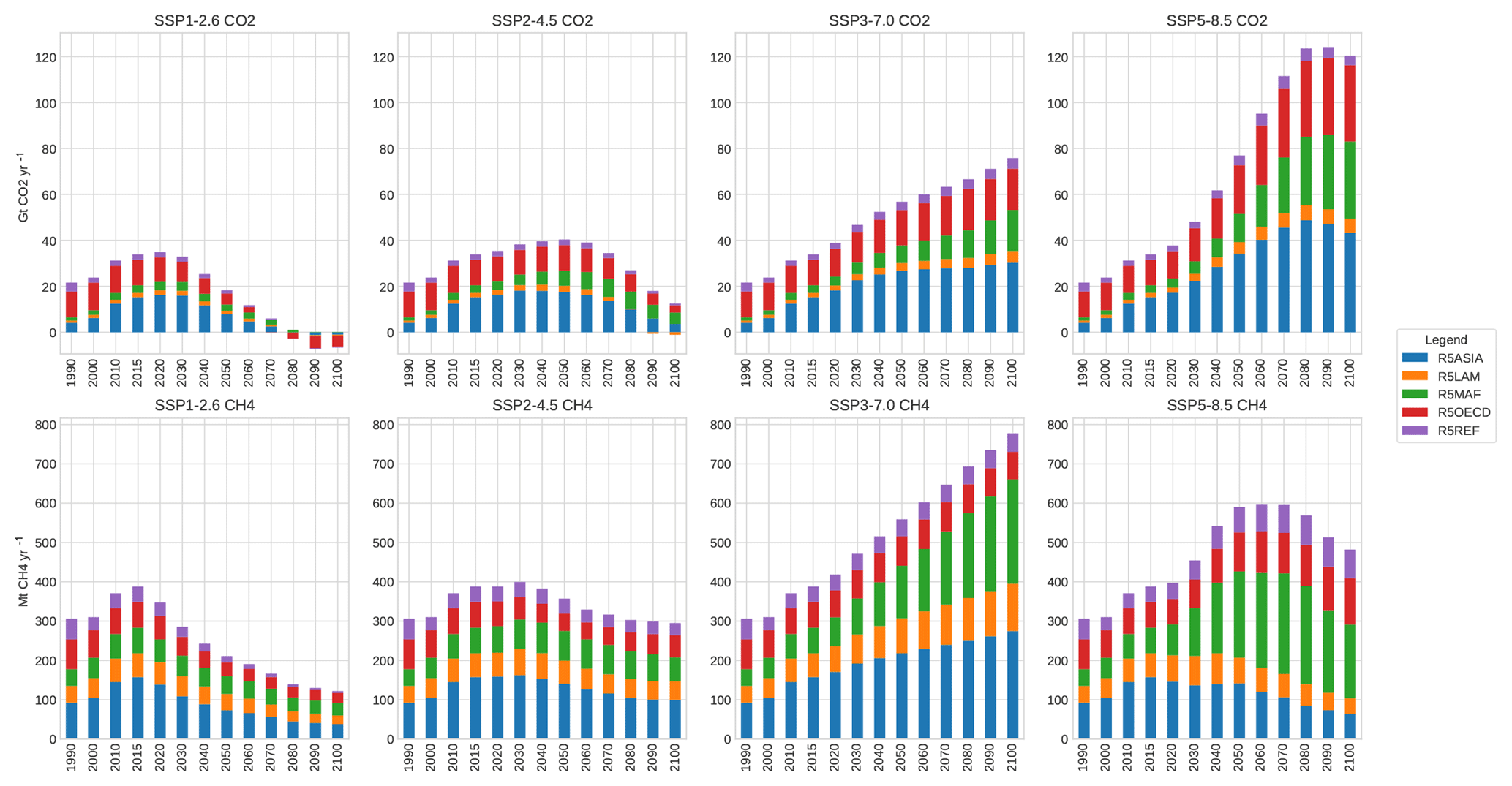
CH4 emissions, resulting from a mix of energy use, food production, and waste disposal, show a different regional breakdown across scenarios. In SSP1-2.6, CH4 emissions are reduced consistently across regions as energy systems transition away from fossil fuel use (notably natural gas) and the husbandry of livestock is curtailed globally. CH4 emissions in other scenarios tend to be dominated by developments in Africa. In SSP5-8.5, for example, emissions in Africa begin to dominate the global profile by mid-century, due largely to expansion of fossil-fuel-based energy production. SSP3 and SSP4 see continued growth in African CH4 emissions across the century, even when global emissions are reduced as in the case of SSP4 scenarios.
CO2 and CH4 are well-mixed climate forcers (Stocker et al., 2013) and thus their spatial variation has a higher impact from a political rather than physical perspective. Aerosols, however, have substantive spatial variability which directly impacts both regional climate forcing via scattering and absorption of solar radiation and cloud formation as well as local and regional air quality. Thus in order to provide climate models with more detailed and meaningful datasets, we downscale emissions trajectories from model regions to individual countries. In most cases, models explicitly represent countries with large shares of emissions (e.g., USA, China, India). MESSAGE-GLOBIOM and REMIND-MAGPIE are notable exceptions; however, their regional aggregations are such that these important countries comprise the bulk of emissions in their aggregate regions (e.g., the MESSAGE-GLOBIOM North American region comprises the USA and Canada). For regions constituted by many countries, country-level emissions are driven largely by bulk region emissions and country GDP in each scenario (per Sect. 2.4). Afterwards, country-level emissions are subsequently mapped to spatial grids (Feng, 2019). We here present global maps of two aerosol species with the strongest implications on future warming, i.e., BC in Fig. 9 and sulfur in Fig. 10. We highlight three cases which have relevant aerosol emissions profiles: SSP1-2.6, which has significantly decreasing emissions over the century, SSP3-7.0, which has the highest aerosol emissions, and SSP3-LowNTCF, which has socioeconomic drivers similar to those of the SSP3 baseline but models the inclusion of policies which seek to limit emissions of near-term climate forcing species.
At present, BC has the highest emissions in China and India due largely to traditional biomass usage in the residential sector and secondarily to transport-related activity. In scenarios of high socioeconomic development and technological progress, such as SSP1-2.6, emissions across countries decline dramatically such that by the end of the century, total emissions in China, for example, are equal to those of the USA today. In almost all countries, BC emissions are nearly eradicated by mid-century while emissions in southeast Asia reach similar levels by the end of the century. In SSP3-7.0, however, emissions from southeast Asia and central Africa increase until the middle of the century as populations grow while still depending on fossil-fuel-heavy energy supply technologies, transportation, and cooking fuels. By the end of the century in SSP3-7.0, global BC emissions are nearly equivalent to the present day (see, e.g., Fig. 5), but these emissions are concentrated largely in central Africa, southeast Asia, and Brazil while they are reduced in North America, Europe, and central Asia. By enacting policies that specifically target near-term climate forcers in SSP3-LowNTCF, the growth of emissions in the developing world is muted by mid-century and is cut by more than half of today's levels (∼9 vs. ∼4 Mt yr−1) by the end of the century. These policies result in similar levels of BC emissions in China as in SSP1-2.6, while most of the additional emissions are driven by activity in India and central Africa due to continued dependence on traditional biomass for cooking and heating.

Figure 9Downscaled and gridded emissions of black carbon at present and in 2050 and 2100 for SSP1-2.6, SSP3-7.0, and SSP3-LowNTCF.
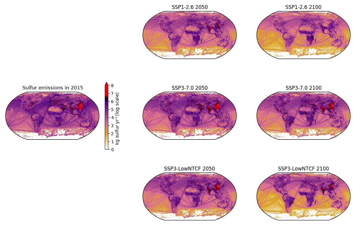
Figure 10Downscaled and gridded emissions of sulfur at present and in 2050 and 2100 for SSP1-2.6, SSP3-7.0, and SSP3-LowNTCF.
The spatial distribution of sulfur emissions varies from that of BC due to large contributions from energy and industrial sectors, and is thus being driven by a country's economic size and composition, as opposed to household activity. Emissions today are largely concentrated in countries having large manufacturing, industrial, and energy supply sectors with heavy reliance on coal, such as China, India, the USA, Russia, and some parts of the Middle East. Again, we observe in SSP1-2.6 a near elimination of sulfur emissions by the end of the century with some continued reliance on sulfur-emitting technologies in India and China in the middle of the century. In SSP3-7.0, although global sulfur emissions over the course of the century peak slightly before reducing to below current levels, increased emissions in southeast Asia offset reductions in emissions elsewhere due to an expanding industrial sector with continued reliance on coal. Notably, emissions in India peak around mid-century before reducing to a magnitude lower than emissions levels today. In the SSP3-LowNTCF scenario, NTCF policies have the added effect of reducing sulfur emissions, resulting in more RF but fewer potential health impacts due to sulfur pollution. By the end of the century in SSP3-LowNTCF, only India, China, and Brazil have nontrivial quantities of emissions at significantly lower magnitudes than today.
We present a suite of nine scenarios of future emissions trajectories of anthropogenic sources, a key deliverable of the ScenarioMIP experiment within CMIP6. IAM results for 14 different emissions species and 13 individual sectors are provided for each scenario with consistent transitions from the historical data used in CMIP6 to future trajectories using automated harmonization before being downscaled to provide higher emissions source spatial detail. Harmonized emissions at global, original native model region, and gridded resolution have been delivered to participating climate teams in CMIP6 for further analysis and study by a number of different MIPs.
Scenarios were selected from a candidate pool of over 40 different SSP realizations such that a range of climate outcomes are represented which provide sufficient spacing between EOC forcing to sample statistically significant global and regional temperature outcomes. Of the nine scenarios, four were selected to match forcing levels previously provided by the RCP scenarios used in CMIP5. RF trajectories are largely comparable between two scenario sets. Five additional scenarios were analyzed in order to enrich the possible studies of physical and climate impact modeling teams as well as support the scientific goals of specific MIPs. The additional scenarios provide both a variety of statistically different EOC climate outcomes as well as enhanced policy and scientific relevance of potential analyses.
These emissions data are now being used in a variety of multi-model climate model studies (e.g., Fiedler et al., 2019), including ScenarioMIP. Identifying sources of uncertainties is a critical component of the larger exercise of CMIP6. As such, it is important that scientists using these datasets for further model input and analysis take care when assessing the uncertainty not only between scenarios but also between model results for a certain scenario. While each scenario is presented by a single model in ScenarioMIP, models have also provided a wider range of results as part of the SSP process.
A multi-model dispersion3 analysis is discussed in Appendix Appendix H in order to provide further insight into the robustness of results of emissions trajectories across models for specific forcing targets. Notably, we observe large disagreement between models for F-gas trajectories (>100 % dispersion by EOC in certain cases); thus uncertainty for these species can be considered large by climate modeling teams. We further observe small but non-negligible EOC dispersion (>20 %) for certain aerosol emissions species, including CO, NH3, OC, and sulfur. In general, dispersion between models of GHG species increases as EOC RF decreases as the wide array of mitigation options chosen to meet these lower climate targets can vary across models. The importance of this measure of uncertainty is also scenario dependent. For example, models in general report low emissions in SSP1 and high emissions in SSP3; thus, the impact of dispersion may have a higher relevance to climate modelers in SSP3 than SSP1.
The ability for other IAM teams to generate and compare results with ScenarioMIP scenarios is also of considerable importance in conjunction with CMIP6 and, after its completion, for further scientific discovery and interpretation of results. As such, we have striven to make openly available all of the tools used in this exercise. The harmonization tool used in this study, Aneris, is provided as an open-source software on GitHub as is the downscaling and gridding methodology. Documentation for both is provided to users online. Such efforts and standardizations not only make the efforts of ScenarioMIP robust and reproducible, but can also prove useful for future exercises integrating a variety of complex models.
The harmonization tool used in this study, Aneris, is available at https://github.com/iiasa/aneris (last access: 8 April 2019) and documentation for using the tool is available at http://software.ene.iiasa.ac.at/aneris/(last access: 8 April 2019). Similarly, the downscaling tool used is available at https://github.com/iiasa/emissions_downscaling (last access: 8 April 2019) and its documentation can be found at https://github.com/iiasa/emissions_downscaling/wiki (last access: 8 April 2019). Model data, both unharmonized and harmonized, are publicly available at the SSP database v1.1 (https://tntcat.iiasa.ac.at/SspDb, last access: 8 April 2019) via the “CMIP6 Emissions” tab while gridded data are available via the ESGF Input4MIPs data repository (https://esgf-node.llnl.gov/projects/input4mips/, last access: 8 April 2019).
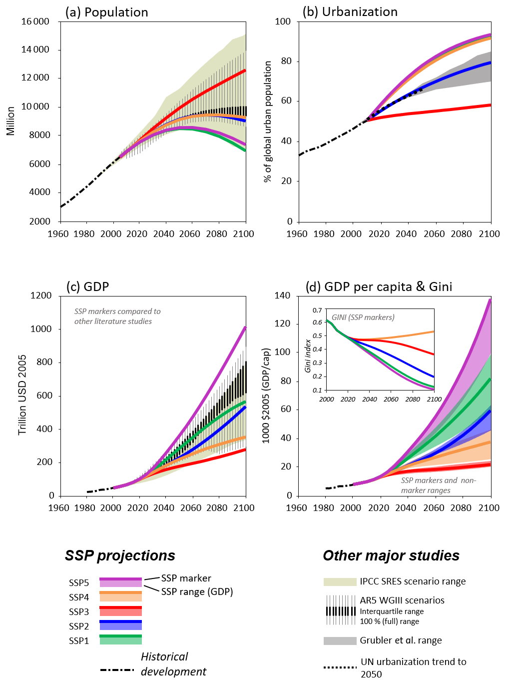
Figure A1The primary socioeconomic assumptions associated with each SSP, including population (KC and Lutz, 2017), urbanization (Jiang and O'Neill, 2017), and GDP (Dellink et al., 2015). The figure is adapted from Riahi et al. (2017) with permission from the authors.
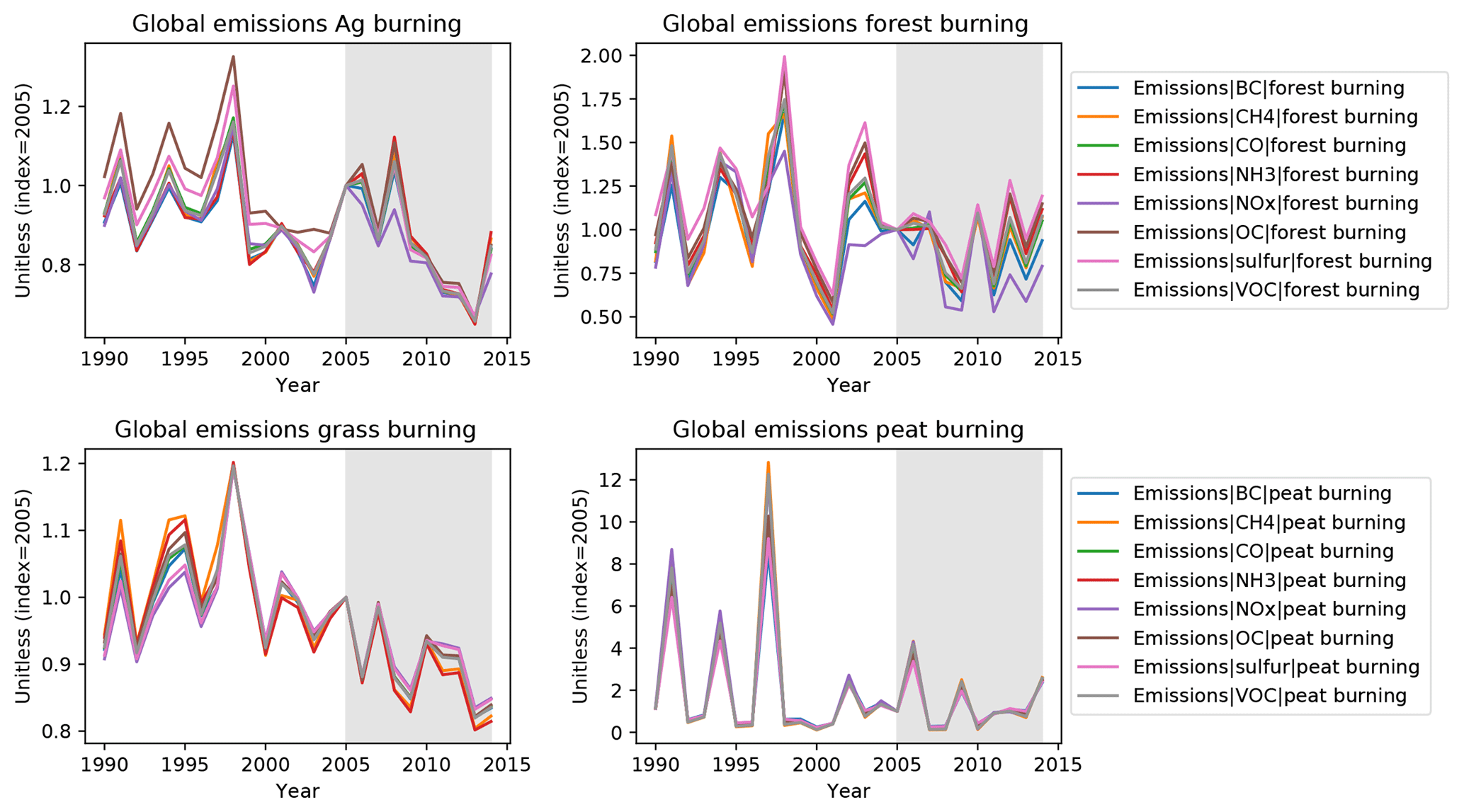
Figure A2Historic values for land-burning emissions from 1990 until 2014. All values for each emissions species are normalized to their value in 2005. The climatological mean window used for harmonization is shown in grey. While decadal trends are present for some sectors, year-on-year trends see large variation.
Table B1The sectoral mapping used to aggregate historical data to a common sectoral definition.
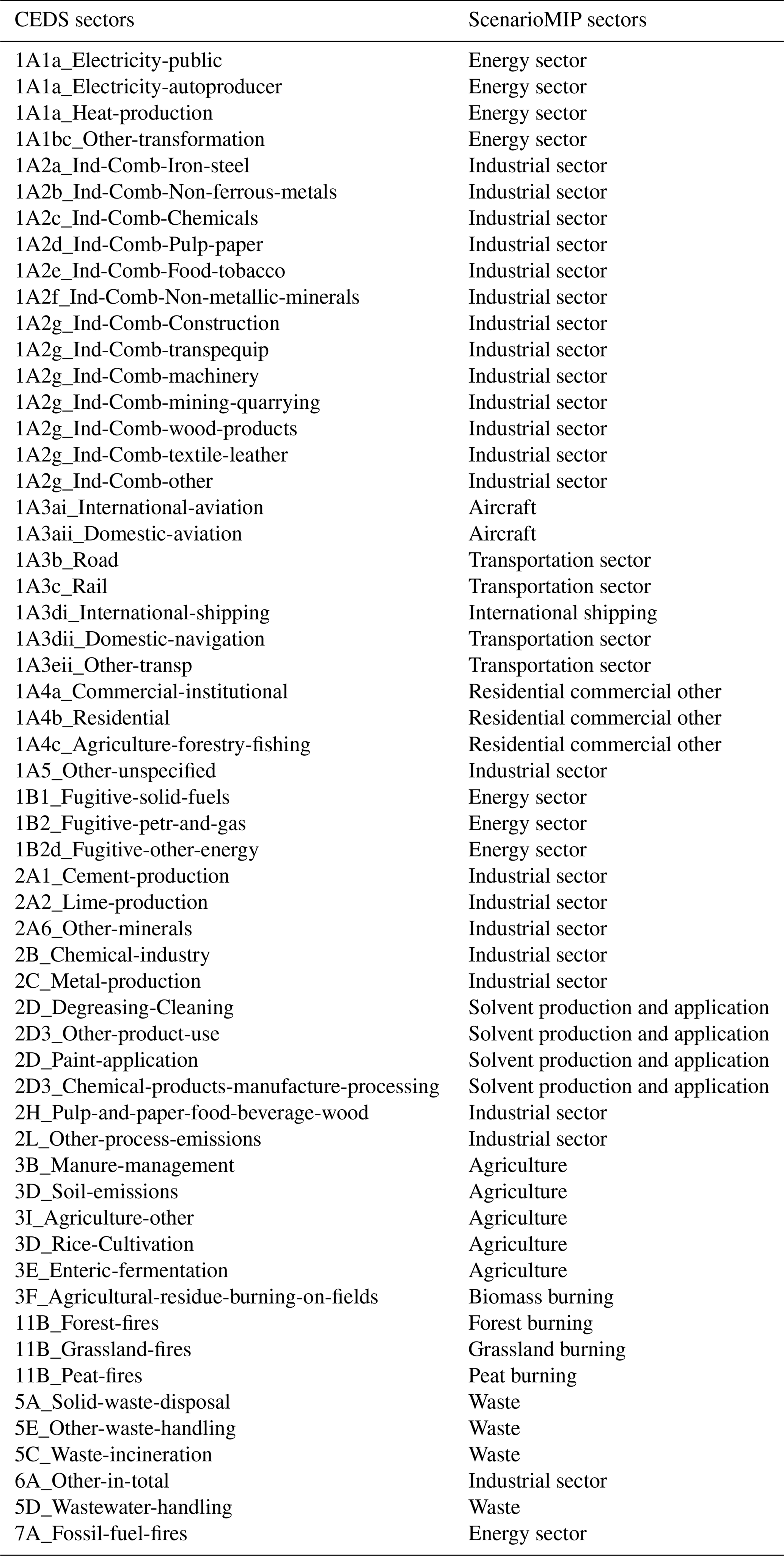
Table B2The sectoral mapping used to aggregate model output data to a common sectoral definition.
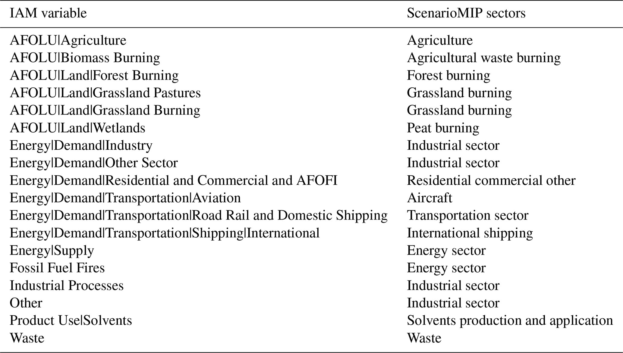
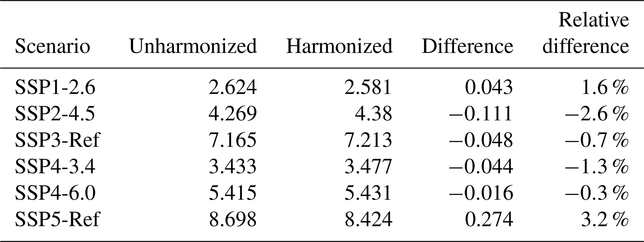
Table B3EOC RF values for unharmonized and harmonized scenario results and differences between the two. The ScenarioMIP design (O'Neill et al., 2016) states that absolute differences must be within ±0.75 W m−2, for which all scenarios fall well within the acceptable value.
The SSP3-LowNTCF scenario utilizes common assumptions with the SSP3-7.0 scenario except in the cases of assumptions regarding near-term climate forcing (NTCF) species emission factors. These differences are designed to compare situations within a SSP3 world in which NTCF-related policies are enacted in the absence of other GHG-related climate policies. Here we list the assumptions additionally made to SSP3-7.0.
-
Regarding CH4, the CH4 emissions' reduction rates in SSP1-26 relative to SSP1 baseline are adopted to SSP3-7.0. This implicitly assumes that SSP3-LowNTCF can reduce CH4 as if SSP1's stringent climate mitigation policy is implemented in the SSP3 world.
-
For air pollutant species (sulfur, NOx, VOC, CO, NH3, BC, and OC), the emissions factors assumed in SSP1 are adopted. This assumption implicitly assumes that SSP1's air pollutant legislation and technological progress can be achieved in the SSP3 world.
-
Other species such as CFC, HFC, SF6, and C2H6 are identical to SSP3 baseline.
Along with these changes, CH4 emissions reduction further changes other air pollutants and GHG emissions drivers. CH4 reduction generates emissions abatement costs, which changes economic outputs in all sectors and household consumption in AIM/CGE. Consequently energy consumption and CO2 emissions in all sectors are affected, which causes small differences between SSP3-7.0 and SSP3-LowNTCF. Not only CO2 but also N2O, CH4, and air pollutants emissions are also affected by these activity level changes, although this indirect effect is relatively minor.
Emissions data were mapped to a spatial grid generally following the methodologies described in Hoesly et al. (2018). A brief description is given here, and a fuller discussion of the gridding process will be provided in Feng (2019). For most anthropogenic sectors, emissions at the level of country and aggregate sector are mapped to a 0.5 ∘C spatial grid by scaling the 2010 base-year country-level spatial pattern. Open-burning emissions from forest fires, grassland burning, and agricultural waste burning on fields are mapped to a spatial grid in the same manner, except that the spatial pattern is taken to be the average from the last 10 years of the historical dataset (e.g., 2005–2014). For each aggregate gridding sector the spatial pattern of emissions within a country does not change over time in the future scenarios. This means that, for example, the ratio of energy-sector NOx emissions from Shaanxi and Beijing provinces in China is constant over time, even though total NOx emissions from China vary over time. Because sectors are mapped to the grid separately, however, total anthropogenic emissions (e.g., sum from all sectors) from any two regions within a country will, in general, not have the same time evolution.
International shipping and aircraft emissions are gridded globally such that the global pattern does not change, only the overall emissions magnitude. One other exception occurs for net negative CO2 emissions. Negative CO2 emissions occur in these models when biomass feedstocks are used together with geologic carbon dioxide capture and storage (CCS). In this case, physically, the emissions are taken out of the atmosphere at the locations where biomass is grown, not at the point of energy consumption. In order to avoid large, unphysical, net negative CO2 point source emissions, net negative CO2 quantities are, therefore, summed globally and mapped to a spatial grid corresponding to 2010 global cropland net primary production (NPP).
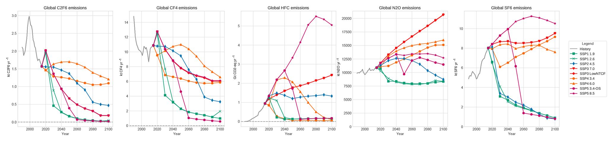
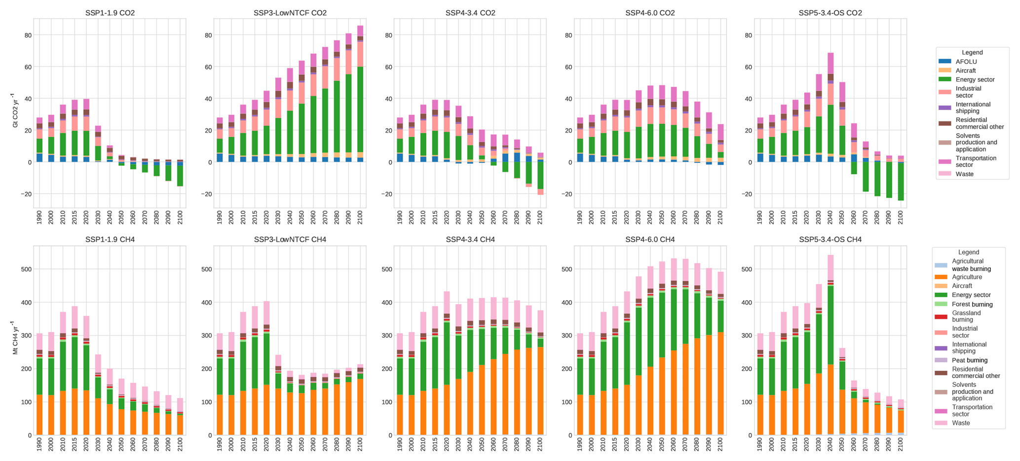
Figure E2Sectoral breakdown for CO2 and CH4 emissions per year for all scenarios analyzed in this study.
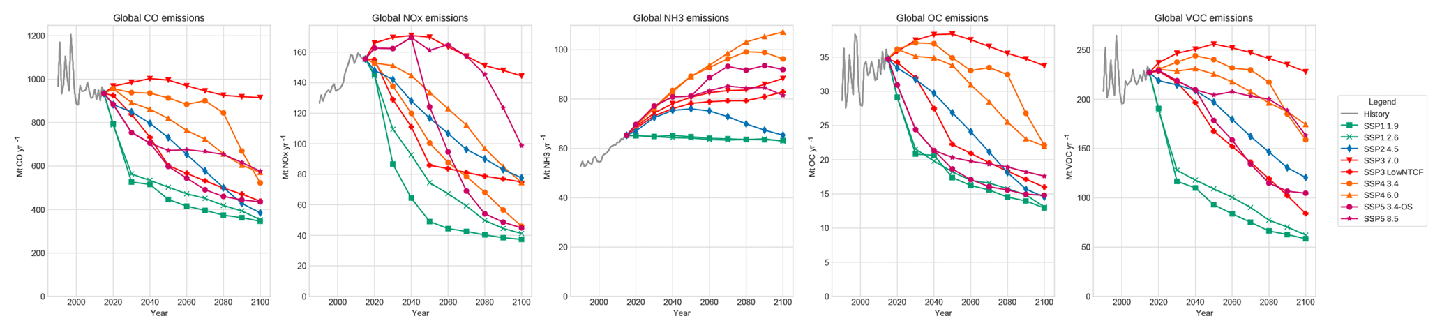
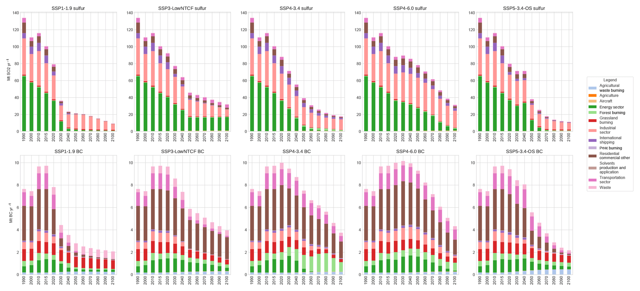
Figure E4Sectoral breakdown for sulfur and BC emissions per year for all scenarios analyzed in this study.
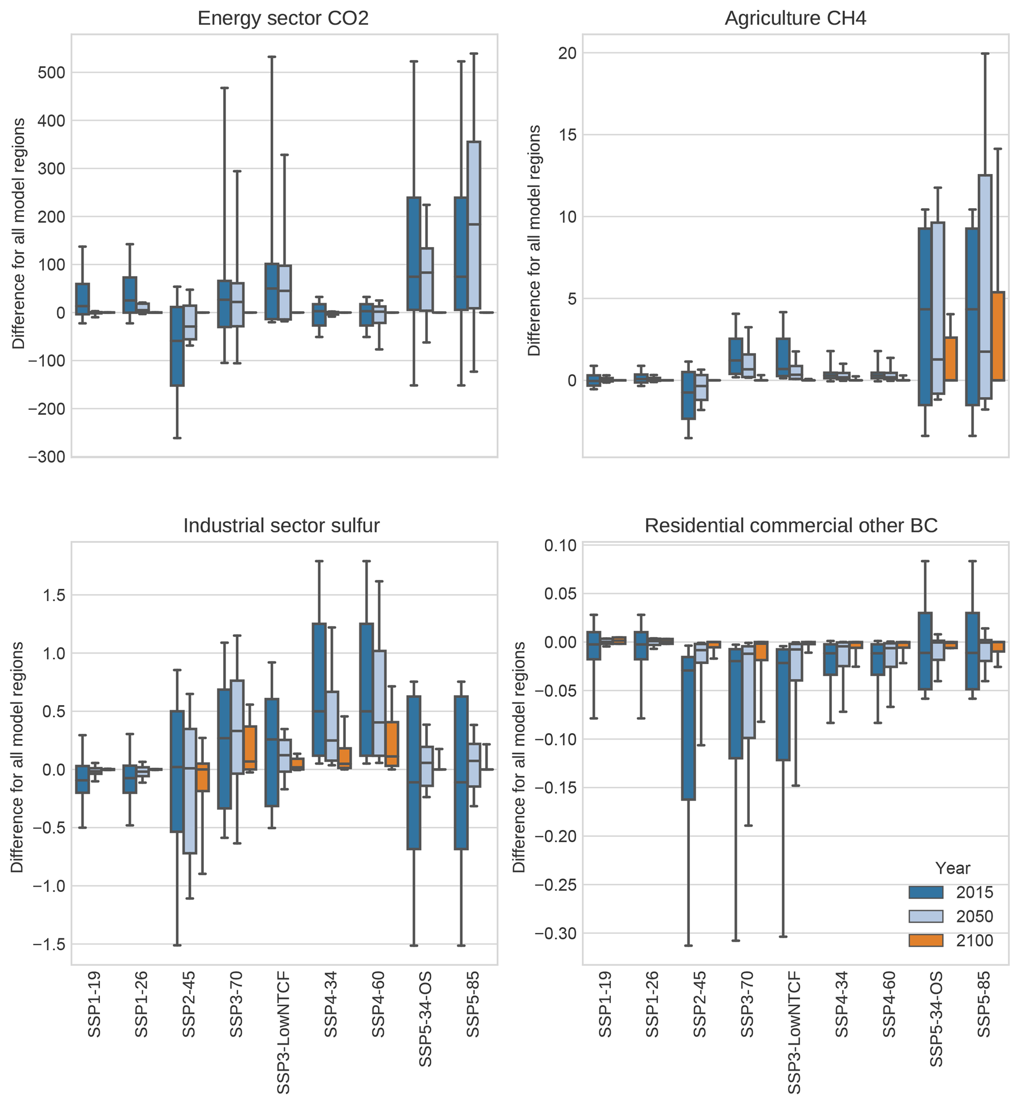
Figure F1The relative difference between harmonized and unharmonized trajectories is shown for the primary sectoral contributor for various emissions species in each scenario. Boxes are comprised of the population of differences for all regions in a given model–scenario combination (see, e.g., Table 3). All box plots show upper and lower quartiles as solid boxes, median values as solid lines, and whiskers extending to the 10th and 90th percentiles. In general, the largest deviations are observed in the base year. The spread of values decreases in time across almost all observations, with the convergence to zero or near zero by EOC.

We here discuss the results of a dispersion analysis measuring the variation in emissions trajectories across models for a given scenario. Dispersion is a measure of the spread of model values for a given global emissions value in a given year. It is calculated in this context as the coefficient of variation (cv) shown in Eq. (H1), which is defined as the ratio of the standard deviation, σ, to mean, μ, of a given population of data.
In order to perform a consistent analysis, we select scenarios for which all participating models provide results: SSP1-2.6, SSP2-4.5, and SSP3-7.0. Scenario data are taken from the available SSP database at https://tntcat.iiasa.ac.at/SspDb (last access: 8 April 2019) (Riahi et al., 2017). Note that dispersion has a nonzero value in the initial year of analysis due to model results not being harmonized in this dataset. We show the dispersion for GHGs (with aggregated F gases) in Fig. H1, individual F gases in Fig. H2, and aerosols in Fig. H3.
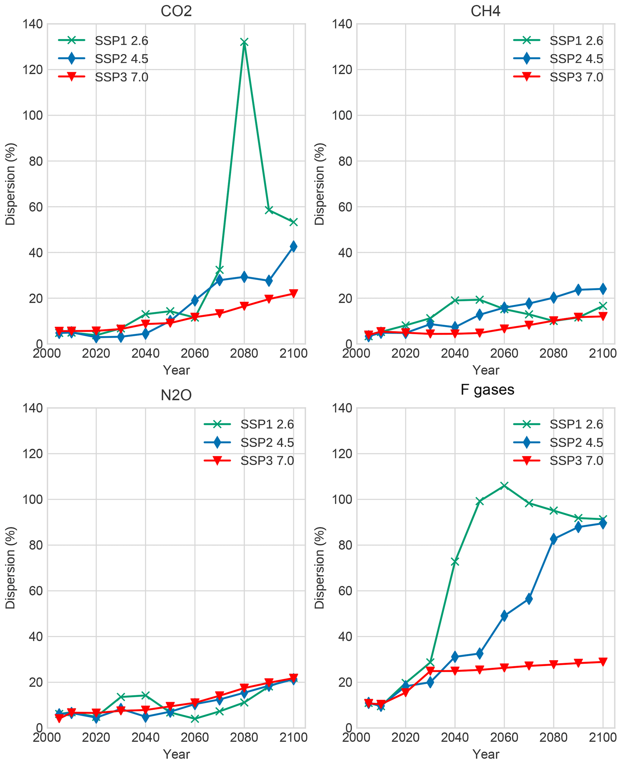
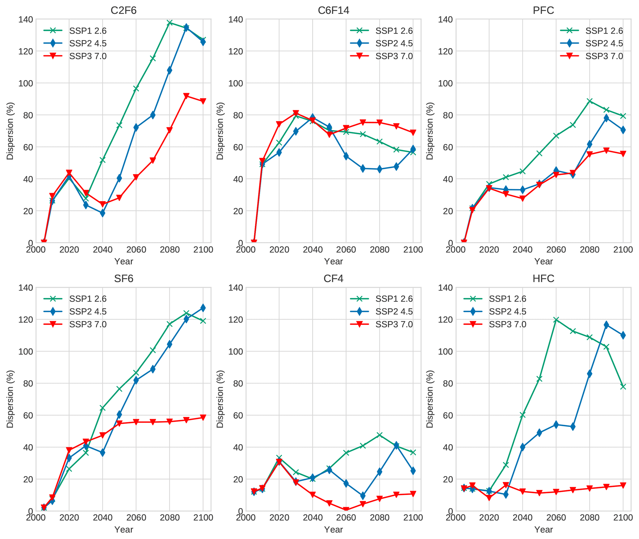
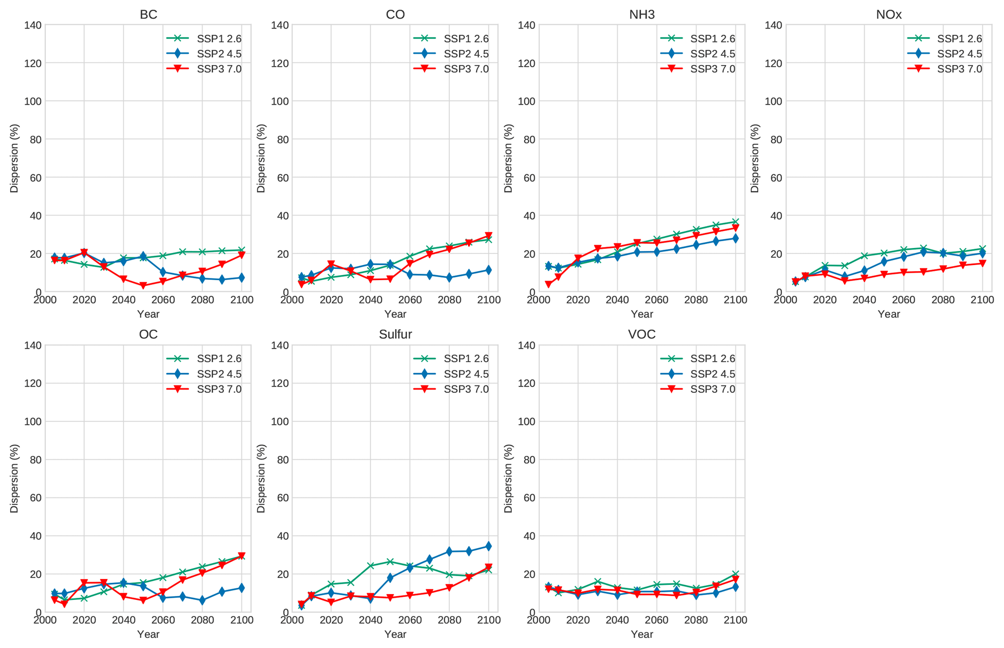
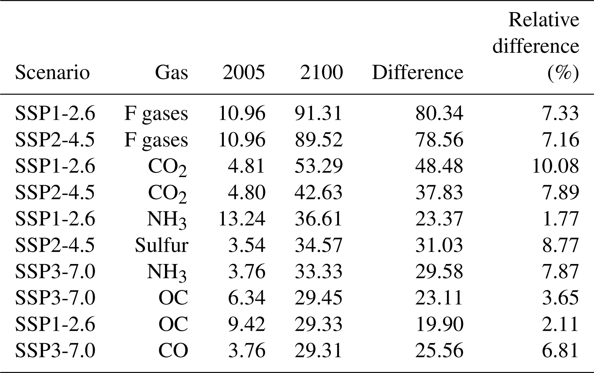
Table H1 shows gas species with the largest values of dispersion. The highest dispersion occurs for F gases, notably C2F6, SF6, and HFCs, implying that models generally do not agree on total magnitudes for these gases. CO2 is also observed to have relatively high dispersion in high-mitigation scenarios. Finally, aerosol species such as NH3, sulfur, and OC show relatively high dispersion values (>30 %). In almost every case, magnitudes of emissions with high dispersion decrease substantially with time; thus this measure, while important for understanding sources of error, may result in small total system error in climate models. There are important scenario–species combinations to take account of, however. First, CO2 dispersion in SSP1-2.6 can be of high consequence because this is a scenario with substantial negative emissions at the end of century. Additionally, users of the data should be aware of the dispersion for aerosols in SSP3, as many aerosol species have large EOC magnitudes, thus showing significant variation across models for these species–scenario combinations.
Table H1The dispersion (cv) for the first modeled period and last modeled period for scenarios with maximum model representation. Here we show the 10 highest EOC dispersion values for a given scenario–species combination.
MG, KR, SS, ShF, GL, EK, DV, MV, and DK contributed to the harmonization process and provided extensive data validation efforts. LF led the downscaling effort assisted by SS and MG. KC, JD, StF, OF, MH, TH, PH, JeH, RH, JiH, AP, ES, and KT contributed scenario data. All authors contributed to the writing of the paper.
The authors declare that they have no conflict of interest.
The authors would like to thank Joeri Rogelj for his thoughtful comments during the development of this paper. This project has received funding from the European Union's Horizon 2020 research and innovation program under grant agreement no. 641816 (CRESCENDO).
This paper was edited by Carlos Sierra and reviewed by three anonymous referees.
Bauer, N., Calvin, K., Emmerling, J., Fricko, O., Fujimori, S., Hilaire, J., Eom, J., Krey, V., Kriegler, E., Mouratiadou, I., de Boer, H. S., van den Berg, M., Carrara, S., Daioglou, V., Drouet, L., Edmonds, J. E., Gernaat, D., Havlik, P., Johnson, N., Klein, D., Kyle, P., Marangoni, G., Masui, T., Pietzcker, R. C., Strubegger, M., Wise, M., Riahi, K., and van Vuuren, D. P.: Shared socio-economic pathways of the energy sector-quantifying the narratives, Global Environ. Change, 42, 316–330, 2017. a, b
Boucher, O., Friedlingstein, P., Collins, B., and Shine, K. P.: The indirect global warming potential and global temperature change potential due to methane oxidation, Environ. Res. Lett., 4, 044007, https://doi.org/10.1088/1748-9326/4/4/044007, 2009. a
BP: BP Statistical Review of World Energy June 2016, Tech. rep., London, 2016. a
Calvin, K., Bond-Lamberty, B., Clarke, L., Edmonds, J., Eom, J., Hartin, C., Kim, S., Kyle, P., Link, R., Moss, R., McJeon, H., Patel, P., Smith, S., Waldhoff, S., and Wise, M.: The SSP4: A world of deepening inequality, Global Environ. Change, 42, 284–296, 2017. a, b
Calvin, K., Patel, P., Clarke, L., Asrar, G., Bond-Lamberty, B., Cui, R. Y., Di Vittorio, A., Dorheim, K., Edmonds, J., Hartin, C., Hejazi, M., Horowitz, R., Iyer, G., Kyle, P., Kim, S., Link, R., McJeon, H., Smith, S. J., Snyder, A., Waldhoff, S., and Wise, M.: GCAM v5.1: representing the linkages between energy, water, land, climate, and economic systems, Geosci. Model Dev., 12, 677–698, https://doi.org/10.5194/gmd-12-677-2019, 2019. a
Carpenter, L., Reimann, S., Burkholder, J., Clerbaux, C., Hall, B., Hossaini, R., Laube, J., and Yvon-Lewis, S.: Scientific Assessment of Ozone Depletion: 2014, World Meteorological Organization Geneva, 2014. a, b
Collins, W. J., Lamarque, J.-F., Schulz, M., Boucher, O., Eyring, V., Hegglin, M. I., Maycock, A., Myhre, G., Prather, M., Shindell, D., and Smith, S. J.: AerChemMIP: quantifying the effects of chemistry and aerosols in CMIP6, Geosci. Model Dev., 10, 585–607, https://doi.org/10.5194/gmd-10-585-2017, 2017. a
Crippa, M., Janssens-Maenhout, G., Dentener, F., Guizzardi, D., Sindelarova, K., Muntean, M., Van Dingenen, R., and Granier, C.: Forty years of improvements in European air quality: regional policy-industry interactions with global impacts, Atmos. Chem. Phys., 16, 3825–3841, https://doi.org/10.5194/acp-16-3825-2016, 2016. a
Dellink, R., Chateau, J., Lanzi, E., and Magné, B.: Long-term economic growth projections in the Shared Socioeconomic Pathways, Global Environ. Change, https://doi.org/10.1016/j.gloenvcha.2015.06.004, 2015. a, b, c
Ehrlich, P. R. and Holdren, J. P.: Impact of population growth, Science, 171, 1212–1217, 1971. a
Etminan, M., Myhre, G., Highwood, E., and Shine, K.: Radiative forcing of carbon dioxide, methane, and nitrous oxide: A significant revision of the methane radiative forcing, Geophys. Res. Lett., 43, 12614–12623, https://doi.org/10.1002/2016GL071930, 2016. a
Eyring, V., Bony, S., Meehl, G. A., Senior, C. A., Stevens, B., Stouffer, R. J., and Taylor, K. E.: Overview of the Coupled Model Intercomparison Project Phase 6 (CMIP6) experimental design and organization, Geosci. Model Dev., 9, 1937–1958, https://doi.org/10.5194/gmd-9-1937-2016, 2016. a
Feng, L.: Gridded Emissions for CMIP6, in preparation, 2019. a, b
Fiedler, S., Stevens, B., Gidden, M., Smith, S. J., Riahi, K., and van Vuuren, D.: First forcing estimates from the future CMIP6 scenarios of anthropogenic aerosol optical properties and an associated Twomey effect, Geosci. Model Dev., 12, 989–1007, https://doi.org/10.5194/gmd-12-989-2019, 2019. a
Fricko, O., Havlik, P., Rogelj, J., Klimont, Z., Gusti, M., Johnson, N., Kolp, P., Strubegger, M., Valin, H., Amann, M., Ermolieva, T., Forsell, N., Herrero, M., Heyes, C., Kindermann, G., Krey, V., McCollum, D. L., Obersteiner, M., Pachauri, S., Rao, S., Schmid, E., Schoepp, W., and Riahi, K.: The marker quantification of the Shared Socioeconomic Pathway 2: A middle-of-the-road scenario for the 21st century, Global Environ. Change, 42, 251–267, https://doi.org/10.1016/j.gloenvcha.2016.06.004, 2017. a, b
Fujimori, S., Hasegawa, T., Masui, T., Takahashi, K., Herran, D. S., Dai, H., Hijioka, Y., and Kainuma, M.: SSP3: AIM implementation of shared socioeconomic pathways, Global Environ. Change, 42, 268–283, 2017. a, b
Gidden, M.: aneris: Harmonization for Integrated Assessment Models, https://doi.org/10.5281/zenodo.802832, 2017. a, b
Gidden, M. J., Fujimori, S., van den Berg, M., Klein, D., Smith, S. J., van Vuuren, D. P., and Riahi, K.: A methodology and implementation of automated emissions harmonization for use in Integrated Assessment Models, Environ. Modell. Softw., 105, 187–200, 2018. a, b, c, d
Gütschow, J., Jeffery, M. L., Gieseke, R., Gebel, R., Stevens, D., Krapp, M., and Rocha, M.: The PRIMAP-hist national historical emissions time series, Earth Syst. Sci. Data, 8, 571–603, https://doi.org/10.5194/essd-8-571-2016, 2016. a, b
Hayhoe, K., Edmonds, J., Kopp, R., LeGrande, A., Sanderson, B., Wehner, M., and Wuebbles, D.: Climate models, scenarios, and projections, in: Climate Science Special Report: Fourth National Climate Assessment, Volume I, 133–160, U.S. Global Change Research Program, Washington D.C., USA, 2017. a
Hoesly, R. M., Smith, S. J., Feng, L., Klimont, Z., Janssens-Maenhout, G., Pitkanen, T., Seibert, J. J., Vu, L., Andres, R. J., Bolt, R. M., Bond, T. C., Dawidowski, L., Kholod, N., Kurokawa, J.-I., Li, M., Liu, L., Lu, Z., Moura, M. C. P., O'Rourke, P. R., and Zhang, Q.: Historical (1750–2014) anthropogenic emissions of reactive gases and aerosols from the Community Emissions Data System (CEDS), Geosci. Model Dev., 11, 369–408, https://doi.org/10.5194/gmd-11-369-2018, 2018. a, b, c
Holmes, C. D., Prather, M. J., Søvde, O. A., and Myhre, G.: Future methane, hydroxyl, and their uncertainties: key climate and emission parameters for future predictions, Atmos. Chem. Phys., 13, 285–302, https://doi.org/10.5194/acp-13-285-2013, 2013. a
Hurtt, G. C.: Scenarios of future land use for CMIP6, Geosci. Model Dev., in preparation, 2019. a
Jiang, L. and O'Neill, B. C.: Global urbanization projections for the Shared Socioeconomic Pathways, Global Environ. Change, 42, 193–199, https://doi.org/https://doi.org/10.1016/j.gloenvcha.2015.03.008, 2017. a, b
Kawase, H., Nagashima, T., Sudo, K., and Nozawa, T.: Future changes in tropospheric ozone under Representative Concentration Pathways (RCPs), Geophys. Res. Lett., 38, L046402, https://doi.org/10.1029/2010GL046402, 2011. a
KC, S. and Lutz, W.: The human core of the shared socioeconomic pathways: Population scenarios by age, sex and level of education for all countries to 2100, Global Environ. Change, 42, 181–192, https://doi.org/https://doi.org/10.1016/j.gloenvcha.2014.06.004, 2017. a, b, c
Klimont, Z., Kupiainen, K., Heyes, C., Purohit, P., Cofala, J., Rafaj, P., Borken-Kleefeld, J., and Schöpp, W.: Global anthropogenic emissions of particulate matter including black carbon, Atmos. Chem. Phys., 17, 8681–8723, https://doi.org/10.5194/acp-17-8681-2017, 2017. a
Kriegler, E., Edmonds, J., Hallegatte, S., Ebi, K. L., Kram, T., Riahi, K., Winkler, H., and Vuuren, D. P. V.: A new scenario framework for climate change research: the concept of shared climate policy assumptions, Clim. Change, 122, 401–414, https://doi.org/10.1007/s10584-013-0971-5, 2014. a
Kriegler, E., Bauer, N., Popp, A., Humpenöder, F., Leimbach, M., Strefler, J., Baumstark, L., Bodirsky, B. L., Hilaire, J., Klein, D., Mouratiadou, I., Weindl, I., Bertram, C., Dietrich, J.-P., Luderer, G., Pehl, M., Pietzcker, R., Piontek, F., Lotze-Campen, H., Biewald, A., Bonsch, M., Giannousakis, A., Kreidenweis, U., Müller, C., Rolinski, S., Schultes, A., Schwanitz, J., Stevanovic, M., Calvin, K., Emmerling, J., Fujimori, S., and Edenhofer, O.: Fossil-fueled development (SSP5): an energy and resource intensive scenario for the 21st century, Global Environ. Change, 42, 297–315, 2017. a, b
Lamarque, J.-F., Shindell, D. T., Josse, B., Young, P. J., Cionni, I., Eyring, V., Bergmann, D., Cameron-Smith, P., Collins, W. J., Doherty, R., Dalsoren, S., Faluvegi, G., Folberth, G., Ghan, S. J., Horowitz, L. W., Lee, Y. H., MacKenzie, I. A., Nagashima, T., Naik, V., Plummer, D., Righi, M., Rumbold, S. T., Schulz, M., Skeie, R. B., Stevenson, D. S., Strode, S., Sudo, K., Szopa, S., Voulgarakis, A., and Zeng, G.: The Atmospheric Chemistry and Climate Model Intercomparison Project (ACCMIP): overview and description of models, simulations and climate diagnostics, Geosci. Model Dev., 6, 179–206, https://doi.org/10.5194/gmd-6-179-2013, 2013. a
Meinshausen, M.: Future greenhouse gas concentrations under the SSP scenarios from 2015 to 2100 and their extensions to 2500, Geosci. Model Dev., in preparation, 2019. a
Meinshausen, M., Raper, S. C. B., and Wigley, T. M. L.: Emulating coupled atmosphere-ocean and carbon cycle models with a simpler model, MAGICC6 – Part 1: Model description and calibration, Atmos. Chem. Phys., 11, 1417–1456, https://doi.org/10.5194/acp-11-1417-2011, 2011a. a
Meinshausen, M., Smith, S. J., Calvin, K., Daniel, J. S., Kainuma, M. L. T., Lamarque, J.-F., Matsumoto, K., Montzka, S. A., Raper, S. C. B., Riahi, K., Thomson, A., Velders, G. J. M., and Vuuren, D. P. P. V.: The RCP greenhouse gas concentrations and their extensions from 1765 to 2300, Clim. Change, 109, 213, https://doi.org/10.1007/s10584-011-0156-z, 2011b. a
Moss, R., Babiker, W., Brinkman, S., Calvo, E., Carter, T., Edmonds, J., Elgizouli, I., Emori, S., Erda, L., Hibbard, K., Jones, R. N., Kainuma, M., Kelleher, J., Lamarque, J. F., Manning, M., Matthews, B., Meehl, J., Meyer, L., Mitchell, J., Nakicenovic, N., ONeill, B., Pichs, R., Riahi, K., Rose, S., Stouffer, R., van Vuuren, D., Weyant, J., Wilbanks, T., vanYpersele, J. P., and Zurek, M.: Towards new scenarios for the analysis of emissions: Climate change, impacts and response strategies, Intergovernmental Panel on Climate Change Secretariat (IPCC), 2008. a
Moss, R. H., Edmonds, J. A., Hibbard, K. A., Manning, M. R., Rose, S. K., van Vuuren, D. P., Carter, T. R., Emori, S., Kainuma, M., Kram, T., Meehl, G. A., Mitchell, J. F. B., Nakicenovic, N., Riahi, K., Smith, S. J., Stouffer, R. J., Thomson, A. M., Weyant, J. P., and Wilbanks, T. J.: The next generation of scenarios for climate change research and assessment, Nature, 463, 747–756, https://doi.org/10.1038/nature08823, 2010. a, b
Nakićenović, N., Alcamo, J., Davis, G., de Vries, B., Fenhann, J., Gaffin, S., Gregory, K., Grübler, A., Jung, T. Y., Kram, T., Lebre La Rovere, E., Michaelis, L., Mori, S., Morita, T., Pepper, W., Pitcher, H., Price, L., Riahi, K., Roehrl, A., Rogner, H. H., Sankovski, A., Schlesinger, M., Shukla, P., Smith, S., Swart, R., van Rooijen, S., Victor, N., and Dadi, Z.: IPCC Special Report on Emissions Scenarios (SRES), Cambridge University Press, UK, available at: http://www.ipcc.ch/ipccreports/sres/emission/index.php?idp=0 (last access: 8 April 2019), 2000. a, b
O'Neill, B. C., Tebaldi, C., van Vuuren, D. P., Eyring, V., Friedlingstein, P., Hurtt, G., Knutti, R., Kriegler, E., Lamarque, J.-F., Lowe, J., Meehl, G. A., Moss, R., Riahi, K., and Sanderson, B. M.: The Scenario Model Intercomparison Project (ScenarioMIP) for CMIP6, Geosci. Model Dev., 9, 3461–3482, https://doi.org/10.5194/gmd-9-3461-2016, 2016. a, b, c, d, e, f, g, h
O'Neill, B. C., Kriegler, E., Riahi, K., Ebi, K. L., Hallegatte, S., Carter, T. R., Mathur, R., and Vuuren, D. P. v.: A new scenario framework for climate change research: the concept of shared socioeconomic pathways, Clim. Change, 122, 387–400, https://doi.org/10.1007/s10584-013-0905-2, 2013. a
O'Neill, B. C., Kriegler, E., Ebi, K. L., Kemp-Benedict, E., Riahi, K., Rothman, D. S., van Ruijven, B. J., van Vuuren, D. P., Birkmann, J., Kok, K., Levy, M., and Solecki, W.: The roads ahead: narratives for shared socioeconomic pathways describing world futures in the 21st century, Global Environ. Change, 42, 169–180, 2017. a
Popp, A., Calvin, K., Fujimori, S., Havlik, P., Humpenöder, F., Stehfest, E., Bodirsky, B. L., Dietrich, J. P., Doelmann, J. C., Gusti, M., and others: Land-use futures in the shared socio-economic pathways, Global Environ. Change, 42, 331–345, 2017. a, b
Rao, S., Klimont, Z., Smith, S. J., Van Dingenen, R., Dentener, F., Bouwman, L., Riahi, K., Amann, M., Bodirsky, B. L., van Vuuren, D. P., Aleluia Reis, L., Calvin, K., Drouet, L., Fricko, O., Fujimori, S., Gernaat, D., Havlik, P., Harmsen, M., Hasegawa, T., Heyes, C., Hilaire, J., Luderer, G., Masui, T., Stehfest, E., Strefler, J., van der Sluis, S., and Tavoni, M.: Future air pollution in the Shared Socio-economic Pathways, Global Environ. Change, 42, 346–358, https://doi.org/10.1016/j.gloenvcha.2016.05.012, 2017. a, b
Riahi, K., Rao, S., Krey, V., Cho, C., Chirkov, V., Fischer, G., Kindermann, G., Nakicenovic, N., and Rafaj, P.: RCP 8.5 – A scenario of comparatively high greenhouse gas emissions, Clim. Change, 109, 33–57, https://doi.org/10.1007/s10584-011-0149-y, 2011. a
Riahi, K., van Vuuren, D. P., Kriegler, E., Edmonds, J., O'Neill, B. C., Fujimori, S., Bauer, N., Calvin, K., Dellink, R., Fricko, O., Lutz, W., Popp, A., Cuaresma, J. C., Kc, S., Leimbach, M., Jiang, L., Kram, T., Rao, S., Emmerling, J., Ebi, K., Hasegawa, T., Havlik, P., Humpenöder, F., Da Silva, L. A., Smith, S., Stehfest, E., Bosetti, V., Eom, J., Gernaat, D., Masui, T., Rogelj, J., Strefler, J., Drouet, L., Krey, V., Luderer, G., Harmsen, M., Takahashi, K., Baumstark, L., Doelman, J. C., Kainuma, M., Klimont, Z., Marangoni, G., Lotze-Campen, H., Obersteiner, M., Tabeau, A., and Tavoni, M.: The Shared Socioeconomic Pathways and their energy, land use, and greenhouse gas emissions implications: An overview, Global Environ. Change, 42, 153–168, https://doi.org/10.1016/j.gloenvcha.2016.05.009, 2017. a, b, c, d
Rogelj, J., Hare, W., Chen, C., and Meinshausen, M.: Discrepancies in historical emissions point to a wider 2020 gap between 2 ∘C benchmarks and aggregated national mitigation pledges, Environ. Res. Lett., 6, 024002, https://doi.org/10.1088/1748-9326/6/2/024002, 2011. a
Rogelj, J., Popp, A., Calvin, K. V., Luderer, G., Emmerling, J., Gernaat, D., Fujimori, S., Strefler, J., Hasegawa, T., Marangoni, G., and others: Scenarios towards limiting global mean temperature increase below 1.5 ∘C, Nat. Clim. Change, 8, 325–332, https://doi.org/10.1038/s41558-018-0091-3, 2018. a
Shindell, D. T., Lamarque, J.-F., Schulz, M., Flanner, M., Jiao, C., Chin, M., Young, P. J., Lee, Y. H., Rotstayn, L., Mahowald, N., Milly, G., Faluvegi, G., Balkanski, Y., Collins, W. J., Conley, A. J., Dalsoren, S., Easter, R., Ghan, S., Horowitz, L., Liu, X., Myhre, G., Nagashima, T., Naik, V., Rumbold, S. T., Skeie, R., Sudo, K., Szopa, S., Takemura, T., Voulgarakis, A., Yoon, J.-H., and Lo, F.: Radiative forcing in the ACCMIP historical and future climate simulations, Atmospheric Chemistry and Physics, 13, 2939–2974, https://doi.org/10.5194/acp-13-2939-2013, 2013. a
Solomon, S., Qin, D., Manning, M., Chen, Z., Marquis, M., Averyt, K. B., Tignor, M., and Miller, H. L. (Eds.): Climate Change 2007 – The Physical Science Basis: Working Group I Contribution to the Fourth Assessment Report of the IPCC, Cambridge University Press, Cambridge, UK and New York, NY, USA, 2007. a, b
Stocker, T. F., Qin, D., Plattner, G., Tignor, M., Allen, S., Boschung, J., Nauels, A., Xia, Y., Bex, V., and Midgley, P.: Climate Change 2013: The Physical Science Basis, Working Group 1 (WG1) Contribution to the Intergovernmental Panel on Climate Change (IPCC) 5th Assessment Report (AR5), Cambridge University Press, Cambridge, UK and New York, NY, USA, 2013. a, b
Stohl, A., Aamaas, B., Amann, M., Baker, L. H., Bellouin, N., Berntsen, T. K., Boucher, O., Cherian, R., Collins, W., Daskalakis, N., Dusinska, M., Eckhardt, S., Fuglestvedt, J. S., Harju, M., Heyes, C., Hodnebrog, Ø., Hao, J., Im, U., Kanakidou, M., Klimont, Z., Kupiainen, K., Law, K. S., Lund, M. T., Maas, R., MacIntosh, C. R., Myhre, G., Myriokefalitakis, S., Olivié, D., Quaas, J., Quennehen, B., Raut, J.-C., Rumbold, S. T., Samset, B. H., Schulz, M., Seland, Ø., Shine, K. P., Skeie, R. B., Wang, S., Yttri, K. E., and Zhu, T.: Evaluating the climate and air quality impacts of short-lived pollutants, Atmos. Chem. Phys., 15, 10529–10566, https://doi.org/10.5194/acp-15-10529-2015, 2015. a
Taylor, K. E., Stouffer, R. J., and Meehl, G. A.: An overview of CMIP5 and the experiment design, B. Am. Meteorol. Soc., 93, 485–498, 2012. a
Tebaldi, C., O'Neill, B., and Lamarque, J.-F.: Sensitivity of regional climate to global temperature and forcing, Environm. Res. Lett., 10, 074001, https://doi.org/10.1088/1748-9326/10/7/074001, 2015. a, b, c
United Nations Treaty Collection: Paris Agreement, available at: https://treaties.un.org/Pages/ViewDetails.aspx?src=TREATY&mtd% sg_no=XXVII-7-d&chapter=27&lang=_en&clang=_en (last access: 8 April 2019), 12 December 2015. a, b
van Marle, M. J. E., Kloster, S., Magi, B. I., Marlon, J. R., Daniau, A.-L., Field, R. D., Arneth, A., Forrest, M., Hantson, S., Kehrwald, N. M., Knorr, W., Lasslop, G., Li, F., Mangeon, S., Yue, C., Kaiser, J. W., and van der Werf, G. R.: Historic global biomass burning emissions for CMIP6 (BB4CMIP) based on merging satellite observations with proxies and fire models (1750–2015), Geosci. Model Dev., 10, 3329–3357, https://doi.org/10.5194/gmd-10-3329-2017, 2017. a
van Vuuren, D. P., Lucas, P. L., and Hilderink, H.: Downscaling drivers of global environmental change: Enabling use of global SRES scenarios at the national and grid levels, Global Environ. Change, 17, 114–130, 2007. a, b
van Vuuren, D. P., Edmonds, J., Kainuma, M., Riahi, K., Thomson, A., Hibbard, K., Hurtt, G. C., Kram, T., Krey, V., Lamarque, J.-F., Masui, T., Meinshausen, M., Nakicenovic, N., Smith, S. J., and Rose, S. K.: The representative concentration pathways: an overview, Clim. Change, 109, 5–31, https://doi.org/10.1007/s10584-011-0148-z, 2011. a, b
van Vuuren, D. P., Kriegler, E., O'Neill, B. C., Ebi, K. L., Riahi, K., Carter, T. R., Edmonds, J., Hallegatte, S., Kram, T., Mathur, R., and Winkler, H.: A new scenario framework for Climate Change Research: scenario matrix architecture, Clim. Change, 122, 373–386, https://doi.org/10.1007/s10584-013-0906-1, 2013. a
van Vuuren, D. P., Stehfest, E., Gernaat, D. E., Doelman, J. C., van den Berg, M., Harmsen, M., de Boer, H. S., Bouwman, L. F., Daioglou, V., Edelenbosch, O. Y., Girod, B., Kram, T., Lassaletta, L., Lucas, P. L., van Meijl, H., Müller, C., van Ruijven, B. J., van der Sluis, S., and Tabeau, A.: Energy, land-use and greenhouse gas emissions trajectories under a green growth paradigm, Global Environ. Change, 42, 237–250, 2017. a, b, c
Velders, G. J., Fahey, D. W., Daniel, J. S., Andersen, S. O., and McFarland, M.: Future atmospheric abundances and climate forcings from scenarios of global and regional hydrofluorocarbon (HFC) emissions, Atmos. Environ., 123, 200–209, 2015. a, b
Walsh, J., Wuebbles, D., Hayhoe, K., Kossin, J., Kunkel, K., Stephens, G., Thorne, P., Vose, R., Wehner, M., Willis, J., Anderson, D., Doney, S., Feely, R., Hennon, P., Kharin, V., Knutson, T., Landerer, F., Lenton, T. Kennedy, J., and Somerville, R.: Our Changing Climate, in: Climate Change Impacts in the United States: The Third National Climate Assessment, 19–67, U.S. Global Change Research Program, Washington D.C., USA, 2014. a
Westervelt, D. M., Conley, A. J., Fiore, A. M., Lamarque, J.-F., Shindell, D. T., Previdi, M., Mascioli, N. R., Faluvegi, G., Correa, G., and Horowitz, L. W.: Connecting regional aerosol emissions reductions to local and remote precipitation responses, Atmospheric Chemistry and Physics, 18, 12461–12475, https://doi.org/10.5194/acp-18-12461-2018, 2018. a
Zheng, B., Tong, D., Li, M., Liu, F., Hong, C., Geng, G., Li, H., Li, X., Peng, L., Qi, J., Yan, L., Zhang, Y., Zhao, H., Zheng, Y., He, K., and Zhang, Q.: Trends in China's anthropogenic emissions since 2010 as the consequence of clean air actions, Atmos. Chem. Phys., 18, 14095–14111, https://doi.org/10.5194/acp-18-14095-2018, 2018. a
For sulfur emissions in China, we include values up to 2017, due to a drastic reduction in these emissions in the most recently available datasets.
Further information regarding the model region definitions is available via the IAMC Wiki at https://www.iamcdocumentation.eu (last access: 8 April 2019) and Calvin et al. (2019).
Dispersion here is defined as the coefficient of variation in model results. The coefficient of variation is defined here as the ratio of the standard deviation to mean (absolute value) of a given population of data. See further discussion in Appendix Appendix H.
- Abstract
- Introduction
- Data and methods
- Results
- Conclusions
- Code and data availability
- Appendix A: Supplement figures
- Appendix B: Supplement tables
- Appendix C: SSP3-LowNTCF scenario assumptions
- Appendix D: Emissions gridding
- Appendix E: Global emissions
- Appendix F: Harmonization
- Appendix G: Regional emissions
- Appendix H: Dispersion analysis
- Author contributions
- Competing interests
- Acknowledgements
- Review statement
- References