H2CM (v1.0): hybrid modeling of global water–carbon cycles constrained by atmospheric and land observations

We present the Hybrid Hydrological Carbon Cycle Model (H2CM) – a global model that couples the terrestrial water and carbon cycles by integrating a process-informed deep learning approach with observational constraints for the water and carbon cycles. H2CM extends the hybrid hydrological model with vegetation (H2MV) to represent key terrestrial carbon fluxes, including gross primary productivity (GPP), autotrophic and heterotrophic respiration at daily resolution and 1° spatial scale. H2CM uses neural networks to learn and predict ecosystem properties governing water and carbon fluxes, such as carbon and water use efficiencies and basal respiration rate. H2CM provides a “reanalysis” of recent land water-carbon cycle variations by combining multiple observational constraints synergistically: on top of hydrological and vegetation data constraints on terrestrial water storage variations, snow water equivalent, evapotranspiration, runoff and fraction of photosynthetically active radiation, the carbon cycle is informed by an observation-based GPP product, and net ecosystem exchange (NEE) from satellite and in situ based atmospheric CO₂ inversion datasets. H2CM reproduces the seasonal and interannual dynamics of carbon fluxes well. H2CM outperforms both purely data-driven models as well as state-of-the-art process-based model ensembles in capturing NEE seasonality, especially in challenging regions such as the South American tropics and Southern Africa. Moreover, H2CM reveals emergent spatial patterns in precipitation use efficiency, light use efficiency, and water-carbon coupling, consistent with empirical ecological understanding. Notably, we show that H2CM learns to represent the rain pulse effect on respiration in dry regions, which is often not well reproduced by global models. H2CM represents a key step toward a new generation of data-driven diagnostic land surface models, with planned extensions to include the energy cycle.

1 Introduction

The water and carbon cycles are critical components of Earth's ecosystems, significantly influencing our understanding of climate, water resources, and carbon dynamics. Previous studies have demonstrated that global water and carbon cycles are strongly interconnected (Jung et al., 2017; Humphrey et al., 2018).

Global water and carbon cycle processes are typically modeled using two main strategies: data-driven modeling and process-based modeling (PBM). Data-driven approaches often involve machine learning (ML) to estimate quantities (e.g., fluxes) related to the water or carbon cycle (Dou et al., 2018; Shi et al., 2024; Tian et al., 2023; Jung et al., 2019, 2020; Nelson et al., 2024). ML can learn from observational data with minimal prior knowledge, relaxing uncertain assumptions and potentially leading to new insights and accurate predictions. This becomes increasingly relevant as the volume of Earth observation data grows (Huntingford et al., 2019; Rolnick et al., 2022; Schneider et al., 2017; Eyring et al., 2024). However, a significant caveat of using ML to explain the Earth system is that these models are very difficult to interpret in terms of learned intermediate processes and mechanisms (e.g., they function as a “black box”). Additionally, they may suffer from extrapolation issues and they do not guarantee adherence to well-established process-knowledge (Shen et al., 2023; Reichstein et al., 2019).

Unlike the ML strategy, PBMs represent process-understanding explicitly and adhere to fundamental laws, such as mass conservation (Le Quéré et al., 2013; Sitch et al., 2015, 2024). By design, PBMs' simulations can output various diagnostic variables that are easy to interpret and help to understand drivers of water-carbon cycle variations in the model. However, PBMs abstract the complex processes governing water and carbon cycles and require numerous assumptions about processes due to incomplete process knowledge. Thus, assumptions and modeling approaches vary across different PBMs, while this uncertainty is reflected in significant inter-model spread of simulations (O'Sullivan et al., 2022). Additionally, unlike ML approaches, PBMs are not designed for fully exploiting the growing volume of Earth observations (Nearing et al., 2021; Shen et al., 2018; Kraft et al., 2022).

A novel approach to modeling global water and carbon cycles – hybrid modeling – has recently emerged. This approach combines ML and PBM within a single framework and aims for leveraging the advantages of both while mitigating their challenges. For instance, hybrid modeling can replace uncertain parameters or process representations of a PBM with ML estimations, while retaining established process knowledge (e.g., mass balance) in the PBM formulations. This can reduce the physical inconsistencies of ML, as ML predictions must pass through process formulations that constrain them to obey process knowledge and maintain physical units. Hybrid modeling also reduces the need for prior assumptions about PBM's uncertain components, if they can be learned from data. Consequently, hybrid modeling allows for leveraging the growing volume of Earth observations through its ML component while maintaining physical plausibility through its PBM component (Eyring et al., 2024; Reichstein et al., 2019; Shen et al., 2023). However, this remains a young and evolving field; global-scale hybrid modeling studies are at the proof-of-concept stage and extensive evaluation and assessment of the plausibility of these models is still needed (Baghirov et al., 2025; Kraft et al., 2022).

A major coupling mechanism between the global water and carbon cycles is related to the carbon-water trade-off during photosynthesis. As plants open their stomata to fix carbon dioxide from the atmosphere they are transpiring water back into the atmosphere (Katul et al., 2012; Heimann and Reichstein, 2008). Soil moisture is another nexus of the water and carbon cycles, as it regulates many processes such as photosynthesis (Humphrey et al., 2018) and heterotrophic respiration (Zhang et al., 2018).

In this study, we introduce the hybrid hydrological-carbon cycle model (H2CM), building on the hybrid hydrological model with vegetation  H2MV, Baghirov et al., 2025). H2MV combines a hydrological model with deep learning (DL) (LeCun et al., 2015), while being constrained by an array of complementary observational data streams on terrestrial water storage (TWS) variations, snow water equivalent (SWE), evapotranspiration (ET), runoff and fraction of photosynthetically active radiation (fAPAR). H2CM extends this approach to include the carbon cycle, where transpiration and gross primary productivity (GPP) are explicitly coupled through neural network (NN) predictions of water use efficiency (WUE). H2CM also represents carbon use efficiency (CUE, defined as the ratio of net to gross primary production) and basal heterotrophic respiration rate (Rb) by NNs to simulate respiration processes. To improve plausibility and causality of NN predictions we couple separate neural networks, which receive individual sets of meaningful inputs for their task, rather than using one large network that receives all inputs to make all estimations. The model simulates spatio-temporal dynamics of GPP and net primary productivity (NPP), heterotrophic respiration (Rh), and thus net ecosystem exchange (NEE) representing the net carbon exchange between land and atmosphere. H2CM's GPP estimations are directly constrained using observation-based data, while NEE estimations are constrained using atmospheric inversion products. Thus, H2CM aims at facilitating a “reanalysis” of carbon-water cycle variations by a joint interpretation of diverse observational data streams based on conceptual process-understanding incorporated into deep learning.

This study has the overall objective to describe and evaluate H2CM. To this end we (1) evaluate the model's performance against withheld data constraints; (2) compare the model's GPP, terrestrial ecosystem respiration (TER), and NEE simulations with state-of-the-art data-driven and process-based models; (3) assess the plausibility of the model's learned global patterns for precipitation, water, carbon, and light use efficiencies; (4) illustrate the model's potential to explain and understand carbon flux variations in the challenging region of Southern Africa.

2 Methods

2.1 H2CM

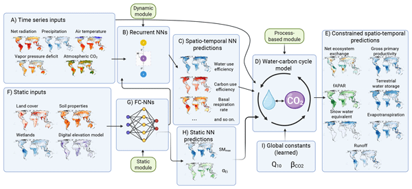
H2CM consists of three primary modules: a static (fully connected) NN module, which generates spatially varying parameters from land cover, soil, and elevation inputs; a dynamic NN module, which produces spatially and temporally varying variables from meteorological forcing; and the process-based (water-carbon cycle) module, which receives the output of the static and dynamic modules, and where fluxes and states are calculated through process equations, which also ensure mass conservation. Note that H2CM's static NN module outputs are at 1° spatial resolution, whereas the dynamic NN and process-based modules' simulations are at 1° spatial and daily temporal resolution.

2.1.1 Hydrological cycle

We utilize the hydrological cycle model component of H2MV (Baghirov et al., 2025) within our model. This hydrological model estimates three primary water storages: snow, soil moisture, and groundwater. It estimates key water fluxes, including snowfall and snowmelt, soil and groundwater recharge, evapotranspiration (divided into transpiration, soil evaporation, and interception evaporation), and runoff (divided into fast and slow runoff) to update these water storages.

In the equations below, parameters with the superscript 〈s,t〉 indicate variables that vary both spatially (s) and temporally (t), while those with the superscript “s” refer solely to spatial variation. Parameters without any superscript represent globally constant parameters (denoted by the Greek letter β or Q₁₀) that do not vary either in space or time and are learned by the neural network.

The main coupling mechanism between water and carbon cycles in H2CM is through linking transpiration and GPP by modelling WUE.

Transpiration (T) is modeled as described by Baghirov et al. (2025):

$$\begin{array}{}\text{(1)}& T^{\langle \mathrm{s},\mathrm{t}\rangle }={\mathrm{fAPAR}}^{\langle \mathrm{s},\mathrm{t}\rangle }\cdot {\mathrm{ET}}_{\mathrm{pot}}^{\langle \mathrm{s},\mathrm{t}\rangle }\cdot {\mathit{\alpha }}_T^{\langle \mathrm{s},\mathrm{t}\rangle }\left(\mathrm{in}\mathrm{mm}{\mathrm{d}}^{-\mathrm{1}}\right),\end{array}$$

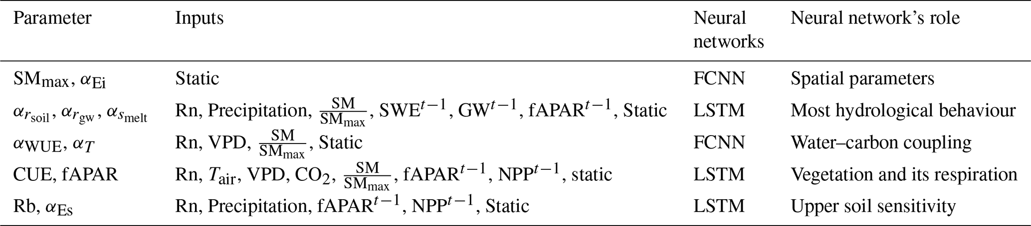
where transpiration is a function of the predicted vegetation state (fAPAR), potential evapotranspiration, and a neural network-learned parameter α_T, which represents effective conductance or stress. The predictions of α_T depend on relative soil moisture, vapor pressure deficit, net radiation, and static variables (Table 1).

Table 1 Guided neural networks: the first column shows the estimated parameters, the second column lists the inputs used in the estimation process, the third column details the types of neural networks used for estimating these parameters, and the last column shows behaviour each neural network controls. α_WUE: water use efficiency without CO₂ fertilisation, CUE: carbon use efficiency, fAPAR: fraction of absorbed photosynthetically active radiation, Rb: Basal respiration rate, FCNN: fully connected neural networks, LSTM: long short-term memory, Rn: net radiation, $\frac{\mathrm{SM}}{{\mathrm{SM}}_{\max }}$: relative soil moisture, SWE: snow water equivalent, GW: groundwater, VPD: vapor pressure deficit, CO₂: atmospheric carbon-dioxide concentration, NPP: net primary productivity. The α parameters that are used in hydrological cycle are introduced in Baghirov et al. (2025).

Parameters such as α_T are explicit NN outputs. During training, the NN predicts α_T from its inputs, and this value – together with variables like fAPAR – is passed to the process-based component to estimate transpiration, which contributes to total ET. Because ET is constrained by observations, training minimizes the loss between predicted and observed ET, thereby adjusting α_T, among other parameters, iteratively. Moreover, α_T is also influenced indirectly through other observational constraints (e.g., TWS, runoff, GPP), so multiple datasets jointly influence its learning. Further details on the hydrological model are available in Baghirov et al. (2025).

2.1.2 Carbon cycle

We employ a simple, conceptual carbon cycle model to estimate carbon cycle fluxes (Fig. 1).

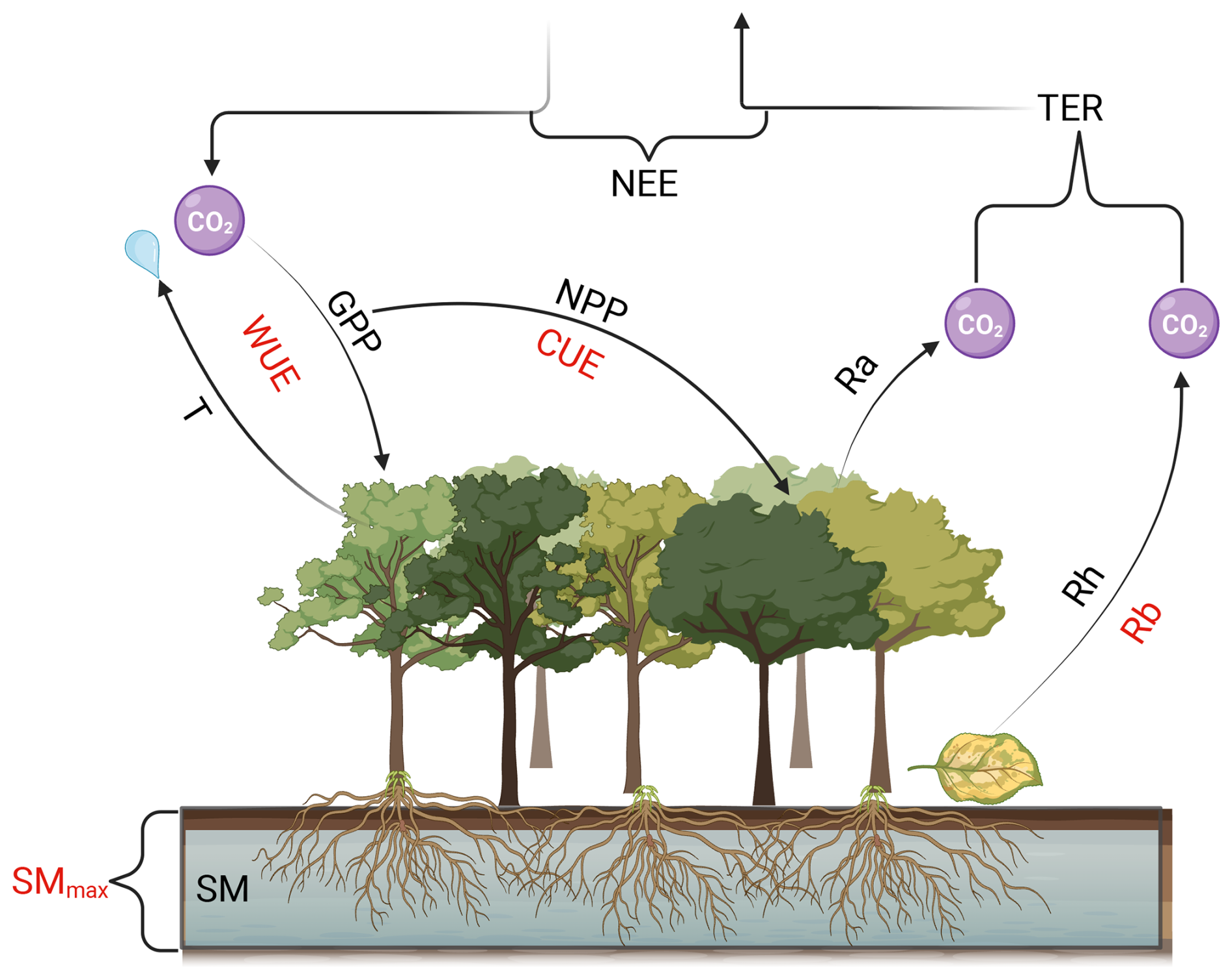
Figure 1 High level overview of the carbon cycle related processes in H2CM: Acronyms above or below the arrows shown in black (e.g., GPP) represent modeled parameters. Acronyms next to the arrows and modelled parameters shown in red (e.g., WUE), indicate parameters directly learned by neural networks to model the corresponding parameter next to the arrow. T: transpiration, WUE: water use efficiency, GPP: gross primary productivity, CUE: carbon use efficiency, NPP: net primary productivity, NEE: net ecosystem exchange, Ra: autotrophic respiration, Rh: heteorotrophic respiration, Rb: basal respiration rate, TER: terrestrial ecosystem respiration, SM_max: maximum soil moisture capacity, SM: soil moisture. Created in BioRender (Baghirov, 2025a).

GPP is the amount of carbon dioxide absorbed by vegetation to produce organic matter through photosynthesis. We model GPP as:

$$\begin{array}{}\text{(2)}& {\mathrm{GPP}}^{\langle \mathrm{s},\mathrm{t}\rangle }=T^{\langle \mathrm{s},\mathrm{t}\rangle }\cdot {\mathit{\alpha }}_{\mathrm{WUE}}^{\langle \mathrm{s},\mathrm{t}\rangle }\cdot {{\mathrm{CO}}_{\mathrm{2}}}^{\langle \mathrm{s},\mathrm{t}\rangle }\cdot {\mathit{\beta }}_{{\mathrm{CO}}_{\mathrm{2}}}\left(\mathrm{in}\mathrm{gC}{\mathrm{m}}^{-\mathrm{2}}{\mathrm{d}}^{-\mathrm{1}}\right)\end{array}$$

where GPP is a function of transpiration T, atmospheric CO₂ concentration, the global constant ${\mathit{\beta }}_{{\mathrm{CO}}_{\mathrm{2}}}$ describing the CO₂ fertilization effect and NN learned α_WUE describing WUE without the CO₂ fertilisation effect. The ${\mathit{\beta }}_{{\mathrm{CO}}_{\mathrm{2}}}$ term is a globally constant, trainable parameter that regulates the strength of the CO₂ fertilization effect on GPP. Although ${\mathit{\beta }}_{{\mathrm{CO}}_{\mathrm{2}}}$ does not explicitly represent a dynamic CO₂ fertilization effect, the model's linear dependence on atmospheric CO₂ interacts with α_WUE which is learned by the neural network as a nonlinear function of vapor pressure deficit, relative soil moisture, net radiation, and static variables (Table 1).

NPP is the net carbon available after autotrophic plant respiration. NPP is modeled as:

$$\begin{array}{}\text{(3)}& {\mathrm{NPP}}^{\langle \mathrm{s},\mathrm{t}\rangle }={\mathrm{GPP}}^{\langle \mathrm{s},\mathrm{t}\rangle }\cdot {\mathrm{CUE}}^{\langle \mathrm{s},\mathrm{t}\rangle }\left(\mathrm{in}\mathrm{gC}{\mathrm{m}}^{-\mathrm{2}}{\mathrm{d}}^{-\mathrm{1}}\right)\end{array}$$

where NPP is a function of GPP and CUE. CUE is directly learned by the NN which receives air temperature, vapor pressure deficit, net radiation, atmospheric CO₂ concentration, relative soil moisture, fAPAR and NPP at previous time step, and static variables (Table 1). Autotrophic respiration is simply calculated as the difference between GPP and NPP.

Heterotrophic respiration, Rh, refers to the process by which non-photosynthetic organisms (e.g., microorganisms) decompose organic matter, releasing carbon dioxide back to the atmosphere. We model Rh using a traditional Q₁₀ function:

$$\begin{array}{}\text{(4)}& {\mathrm{Rh}}^{\langle \mathrm{s},\mathrm{t}\rangle }=Q_{\mathrm{10}}^{\frac{T_{\mathrm{air}}^{\langle \mathrm{s},\mathrm{t}\rangle }-T_{\mathrm{ref}}}{\mathrm{10}}}\cdot {\mathrm{Rb}}^{\langle \mathrm{s},\mathrm{t}\rangle }\left(\mathrm{in}\mathrm{gC}{\mathrm{m}}^{-\mathrm{2}}{\mathrm{d}}^{-\mathrm{1}}\right)\end{array}$$

where Q₁₀, a global constant learned by the NN, describes the temperature sensitivity factor, indicating by which factor respiration increases with a 10 °C rise in air temperature. T_air is the current air temperature at time t, T_ref is the reference temperature set to 15 °C), and Rb is the basal respiration rate essentially representing the availability of carbon for Rh and it is learned by a recurrent NN as a function of precipitation, net radiation, fAPAR and NPP at previous time step, and static variables (Table 1). TER is the sum between autotrophic (Ra) and heteorotrophic (Rh) respiration representing the total amount of carbon dioxide being respired to the atmosphere. NEE is calculated as the difference between TER and GPP, where negative values indicate a land carbon sink.

2.1.3 Overview of the hybrid architecture

Figure 2 illustrates the overall architecture of H2CM:

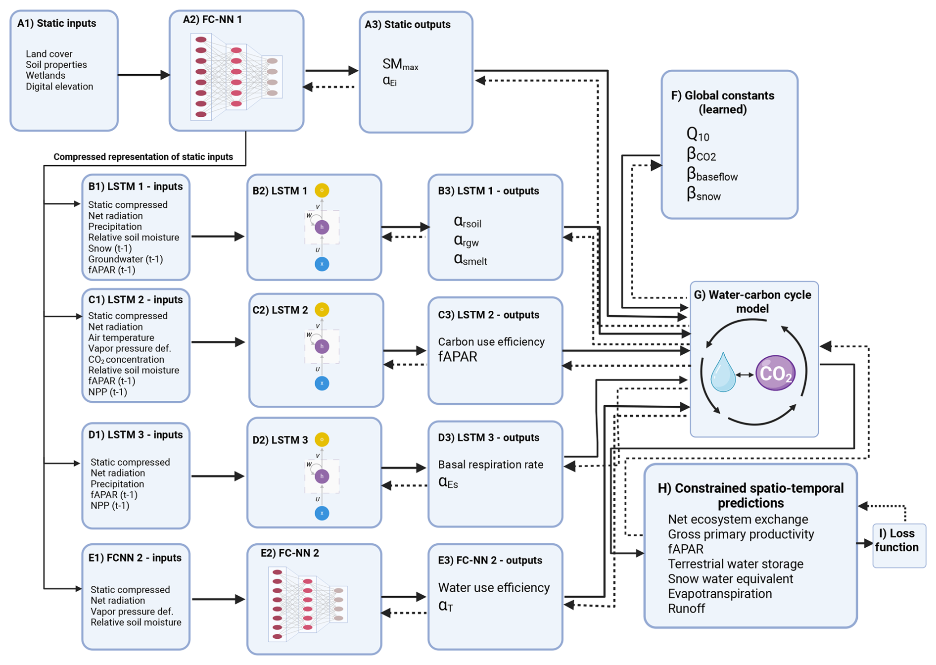
Figure 2 Overview of the H2CM framework. Static inputs (e.g., land cover, soil, elevation) are processed through a fully connected neural network (two hidden layers: 150 and 12 units) to generate compressed static features. These features feed into three LSTM networks (each with one hidden layer of 100 units) and an additional fully connected network that predict spatio-temporal parameters regulating hydrological and carbon processes, including α_rsoil, α_rgw, α_smelt, α_Es, α_Ei, and α_T. Globally learned constants (Q₁₀, ${\mathit{\beta }}_{{\mathrm{CO}}_{\mathrm{2}}}$, β_baseflow, β_snow) control temperature sensitivity, CO₂ fertilization, baseflow recession, and snow corrections. Outputs from all subnetworks are coupled through a differentiable, mass-balanced water–carbon process model. The process layer produces water fluxes and storages and carbon fluxes, some of which are directly constrained by observations, including NEE, GPP, fAPAR, TWS, SWE, ET, and runoff. The dashed lines represent backpropagation used to train H2CM. Created in BioRender (Baghirov, 2026c).

• A.

  Static inputs and compression. Panel A1 represents the static environmental inputs, including land cover, soil properties, wetland extent, and digital elevation. These features are passed through a fully connected neural network (FC-NN 1; A2) that compresses spatially varying but temporally invariant information into a latent vector. FC-NN 1 has two hidden layers with 150 and 12 units, respectively. The 12-unit latent vector is used as compressed static features and serves as a shared input to all dynamic sequence layers. The outputs of this static network (A3) include spatially varying parameters such as maximum soil moisture capacity (SM_max) and α_Ei controlling interception evaporation.

• B–E.

  Dynamic sequence models. H2CM includes three long short-term memory (LSTM) networks and an additional fully connected neural network (FC-NN 2) to model time-varying processes. Each LSTM contains one hidden layer with 100 units and is connected to a small fully connected layer that transforms hidden states into physically interpretable parameters. These dynamic modules produce spatio-temporal predictions:

  • LSTM 1 (B1–B3): receives the compressed static features together with dynamic drivers such as net radiation, precipitation, relative soil moisture, snow, groundwater, and fAPAR at time t−1. It predicts coefficients (α_rsoil, α_rgw, α_smelt) that control soil recharge, groundwater recharge, and snowmelt processes.

  • LSTM 2 (C1–C3): takes inputs including the static compressed vector, air temperature, vapor pressure deficit, CO₂ concentration, relative soil moisture, and fAPAR and NPP at time t−1. It estimates carbon use efficiency and fAPAR.

  • LSTM 3 (D1–D3): uses static compressed features, net radiation, precipitation, fAPAR, and NPP at time t−1 to predict the basal respiration rate and α_Es parameter that controls soil evaporation.

  • FC-NN 2 (E1–E3): a fully connected neural network with two hidden layers (150 and 12 units) that predicts water use efficiency and the α_T parameter, which represents effective conductance or stress response.

• F.

  Global constants (learned). A set of globally learned parameters (Q₁₀, ${\mathit{\beta }}_{{\mathrm{CO}}_{\mathrm{2}}}$, β_baseflow, β_snow) provide scaling relationships for temperature sensitivity of respiration, CO₂ fertilization, baseflow recession, and correction of snowfall.

• G.

  Coupled water–carbon cycle model. The outputs from the static and dynamic subnetworks are passed to a differentiable, process-based water–carbon cycle model that enforces mass balance between fluxes. This model represents the physical coupling between hydrological and carbon processes, ensuring consistency between water storage, evapotranspiration, carbon assimilation, and respiration.

• H.

  Constrained spatio-temporal predictions. During training, all components of the hybrid architecture are optimized jointly, including the static and dynamic neural subnetworks and the differentiable process-based water–carbon cycle model. Gradients are propagated through the full model from the loss function back to the trainable parameters, so that all trainable components are updated simultaneously. The neural network components generate spatially and spatio-temporally varying parameters that are passed into the process model, which produces simulated water fluxes and storages and carbon fluxes. Some of these outputs (net ecosystem exchange, gross primary productivity, fAPAR, terrestrial water storage, snow water equivalent, evapotranspiration, and runoff) are compared against observational targets through a composite loss function (I). Because the process-based component is fully differentiable, gradients of the loss propagate through the process equations back to the neural subnetworks via automatic differentiation (dashed arrows in Fig. 2). This enables the networks to learn physically consistent parameterizations that minimize discrepancies between modeled and observed dynamics.

When we integrate the carbon cycle with the hydrological cycle from H2MV, the number of NN predicted parameters and inputs to the model increases. This expansion raises the risk of the NN component making estimations based on unreasonable relationships, known as short-cut learning (Geirhos et al., 2020). This issue arises due to potential covariations among the inputs, where different inputs or their combinations might be used to estimate certain parameters, even if such associations are implausible based on established process knowledge.

To address this, we `guide' NNs by ensuring they learn from plausible inputs when estimating specific parameters. Instead of employing a single large NN to predict all parameters simultaneously, which is a common approach, we divide the neural networks into groups. Each group is restricted to learning from plausible relationships, enhancing the reliability of the model's predictions (Table 1 and Fig. 2).

2.2 Model optimization

2.2.1 Cross validation (CV)

To evaluate the generalizability of H2CM, we use a 10-fold cross-validation (CV) setup. For this purpose, the spatial domain is divided into 10 folds composed of different grid cells. We then train 10 separate models, each time leaving out one fold of grid cells as the validation set and using the remaining folds for training. The training set is used to optimize the model, while the validation fold is exclusively for hyperparameter tuning, such as selecting the learning rate, and for early stopping. Furthermore, we keep a separate set of grid cells as a testing set, which is used only after training to assess the model's performance and generalizability. Importantly, the testing set is never exposed to the models during the training phase (Fig. A1).

We divide the global data into training, validation, and testing sets using a spatial-only splitting method (Fig. A1). This approach ensures that different grid cells are included in each of the training, validation, and testing sets. To address spatial autocorrelation among grid cells, we implement a spatial blocking technique as recommended by Roberts et al. (2017). In this approach, “blocks” refer to spatially contiguous groups of 5°×5° grid cells (25 grid cells in total) that are treated as single sampling units. These blocks are randomly selected from the global data, ensuring that the majority of the data (approximately 80 % of the grid cells) is allocated to the training set. The remaining ∼20 % of the data is reserved for validation and testing. In practice, each of the 10 cross-validation folds contains roughly $\mathrm{1}/\mathrm{11}$ of the total data for validation, while $\sim \mathrm{1}/\mathrm{11}$ of the data is held out as a fixed testing set for final evaluation. The random selection of blocks also ensures that the training, validation, and testing sets approximately represent grid cells from all continents.

This split is crucial for accurately testing the model's generalizability on unseen testing grid cells and helps in understanding potential overfitting to the training data. Ideally, testing on both spatial and temporal dimensions, known as spatio-temporal splitting, would provide a more rigorous assessment. However, with the current set-up implementing proper time splitting for cross-validation is not feasible due to inconsistent and limited temporal coverage across different data constraints (Table 2). To assess the model's generalizability across both space and time, we conducted an additional experiment in which the model was trained using data from 2001 to 2017 and evaluated on the subsequent two years (2018–2019; Appendix C). The results show qualitative agreement with the spatial CV setup, thereby justifying its validity in this study.

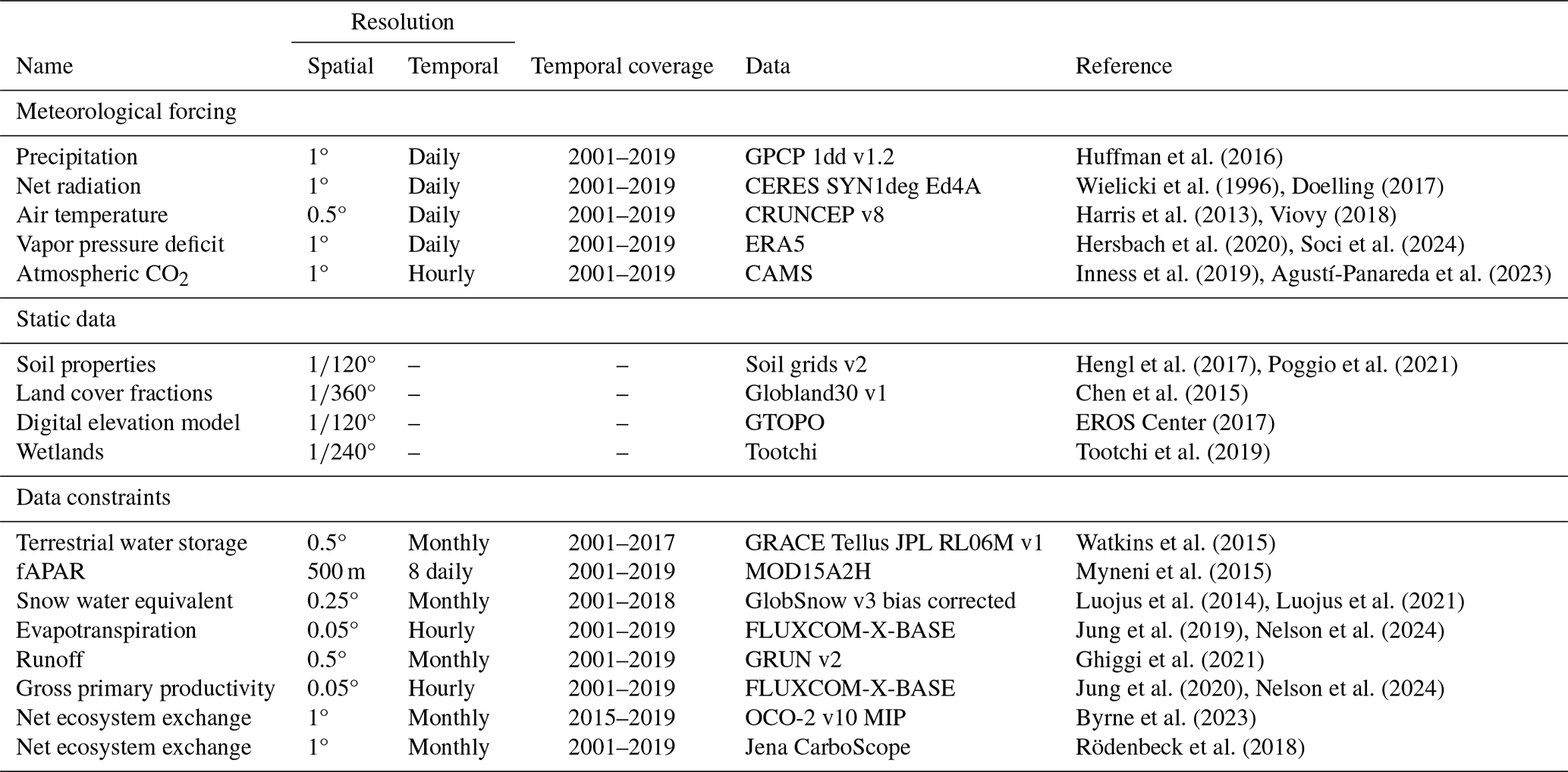
Huffman et al. (2016)Wielicki et al. (1996)Doelling (2017)Harris et al. (2013)Viovy (2018)Hersbach et al. (2020)Soci et al. (2024)Inness et al. (2019)Agustí-Panareda et al. (2023)Hengl et al. (2017)Poggio et al. (2021)Chen et al. (2015)EROS Center (2017)Tootchi et al. (2019)Watkins et al. (2015)Myneni et al. (2015)Luojus et al. (2014)Luojus et al. (2021)Jung et al. (2019)Nelson et al. (2024)Ghiggi et al. (2021)Jung et al. (2020)Nelson et al. (2024)Byrne et al. (2023)Rödenbeck et al. (2018)

Table 2 Overview of datasets: meteorological forcings, static inputs, and data/observational constraints. All temporally varying constraints were aggregated to monthly resolution. The Resolution column lists the original (native) resolution of each dataset.

2.2.2 Loss function

We use the mean squared error (MSE) as the loss function, following the approach in Baghirov et al. (2025). The loss function MSE

$$\begin{array}{}\text{(5)}& L(X,\mathrm{\Theta },\mathit{\beta })={\displaystyle \frac{\mathrm{1}}{N_{\mathrm{c}}}}\sum _{\mathrm{c}=\mathrm{1}}^{\mathrm{C}}\sum _{i=\mathrm{1}}^{N_{\mathrm{c}}}{\left(y_{\mathrm{c},i}-{\widehat{y}}_{\mathrm{c},i}\right)}^{\mathrm{2}}\end{array}$$

evaluates the model's performance based on the inputs X, the neural network weights Θ, and the global constants β. In this context, C denotes the number of data constraints, N_c is the number of data points for each constraint c, and y_c,i and ${\widehat{y}}_{\mathrm{c},i}$ represent the observed and predicted values for the constraint c, respectively. Throughout the training process, Θ and β are adjusted to minimize the overall loss L. Note that we apply a Z-transformation to predictions and observations before computing the loss. This standardizes each variable by subtracting its mean and dividing by its standard deviation, removing the effect of different units and balancing the contributions of each data constraint to the total loss.

The loss function combines all data constraints into a single objective, where MSE is computed by concatenating the data across grid cells and monthly data for each variable. The only exception is for the data constraint on long-term NEE from CarboScope. In situ–based inversions such as CarboScope are generally more robust when averaged globally but become increasingly uncertain at the grid-cell level. Therefore, we first compute the spatial mean of both CarboScope and H2CM NEE monthly anomalies during training within each batch (subset of training samples processed together in one optimization step). This yields time series of spatial averages for which we calculate the loss.

2.2.3 Model training

We use the strategy outlined by Baghirov et al. (2025) to optimize H2CM for each CV fold separately, which includes utilizing the Adam optimizer (Kingma and Ba, 2014). We set the initial learning rate to 0.005 and used a step-wise learning-rate scheduler (StepLR; Paszke et al., 2019) that decays the rate by a fixed factor at fixed epoch intervals. Hyperparameters were tuned by training multiple model variants and selecting the configuration that achieved strong validation performance with stable training. During training, all inputs to the neural networks are standardized using Z-transformation (so deviations from the mean are preserved in standardized units). We also implement early stopping, a technique that monitors both validation and training losses. This approach halts further training if the model's performance on the validation set either declines or remains unchanged, thereby preventing overfitting to the training data. Throughout training, we keep track of the validation loss and select the final model based on the smallest total loss observed on the validation set. This selected model is then used for making final predictions, such as on the testing set.

2.3 Datasets

Our model receives meteorological time series data for each grid-cell, including precipitation, net radiation, air temperature, vapor pressure deficit, and the atmospheric concentration of CO₂, as inputs (Table 2). We use net radiation as a single forcing term rather than separately prescribing shortwave and longwave components. This simplification leverages the strong empirical correlation between shortwave and net radiation at daily scales (Jung et al., 2024). Additionally, we incorporate static inputs, which vary only between grid-cells that consist of soil properties, land cover fractions, elevation, and wetlands, as described in Baghirov et al. (2025). In general, we selected meteorological and static datasets that are widely used in the community, quality-checked, and offer the best compromise between spatial/temporal resolution and observational accuracy for each variable.

All meteorological forcing and data constraints were aggregated to a 1° spatial resolution. The spatial resolutions of static inputs were aggregated to $\mathrm{1}/\mathrm{30}$°. Meteorological forcing data are maintained in their native daily temporal resolutions, while a monthly temporal resolution is applied to the data constraints.

Throughout, we use “data constraints” to denote data-driven constraints implemented as observation-based loss terms using TWS, SWE, ET, runoff, fAPAR, GPP, and NEE (Table 2). These terms guide the model's predictions but are not physically defined hard bounds or conservation laws. Physical constraints (e.g., mass balance) are enforced by the process-oriented component of the model.

We use the OCO-2 LNLGIS atmospheric inversion MIP (v10) ensemble median to constrain our estimations of NEE at 1° spatial resolution for the period 2015–2020, which uses satellite column and in-situ CO₂ observations jointly. Additionally, we use CarboScope (in-situ based NEE inversion product) to constrain the long-term spatial average monthly anomalies of NEE estimations. Both OCO-2 MIP and CarboScope estimate the carbon exchange, which includes contributions from fire emissions that we do not model. Therefore, we use fire emission data from GFED (v4) (Chen et al., 2023) to subtract fire emissions from OCO-2 and CarboScope inversions. We only use the mean seasonal cycle of GPP and ET from FLUXCOM-X-BASE, and runoff from GRUN to constrain the seasonality of our simulations (Table 2), due to caveats of representing interannual variability of these data products (Ghiggi et al., 2019; Jung et al., 2019, 2020; Nelson et al., 2024).

Additionally, we apply a soft constraint on the spatial distribution of mean annual CUE (NPP/GPP), using the TRENDY (v11) ensemble median of global process-oriented ecosystem models (Sitch et al., 2024) as data constraint. This helps to constrain plausible relative contributions of autotrophic and heterotrophic respiration in H2CM. Note that this step only constrains the magnitude of mean CUE based on theoretical expectations, while temporal variations of CUE emerge from training H2CM.

2.4 Model evaluation

We assess our model's performance by utilizing the root mean square error (RMSE), Pearson's correlation coefficient (r), and the standard deviation ratio (SDR), which compares the predicted standard deviation to the observed standard deviation. These metrics are also calculated based on a decomposition into the mean seasonal cycle (MSC) and monthly anomalies (A).

We calculate MSC as:

$$\begin{array}{}\text{(6)}& \mathrm{MSC}\left(m\right)={\displaystyle \frac{\mathrm{1}}{Y}}\sum _{\mathrm{y}=\mathrm{1}}^{\mathrm{Y}}{p}_{\mathrm{m},\mathrm{y}}\end{array}$$

where p_m,y denotes the predicted or observed variable for month m and year y, and Y represents the total number of years.

The monthly anomaly (A(m,y)) represents the deviation of a given month's value from its mean seasonal cycle:

$$\begin{array}{}\text{(7)}& A(m,y)=p_{\mathrm{m},\mathrm{y}}-\mathrm{MSC}\left(m\right)\end{array}$$

where p_m,y represents the estimated or observed variable for a certain month m and year y, and MSC(m) denotes MSC for that specific month m.

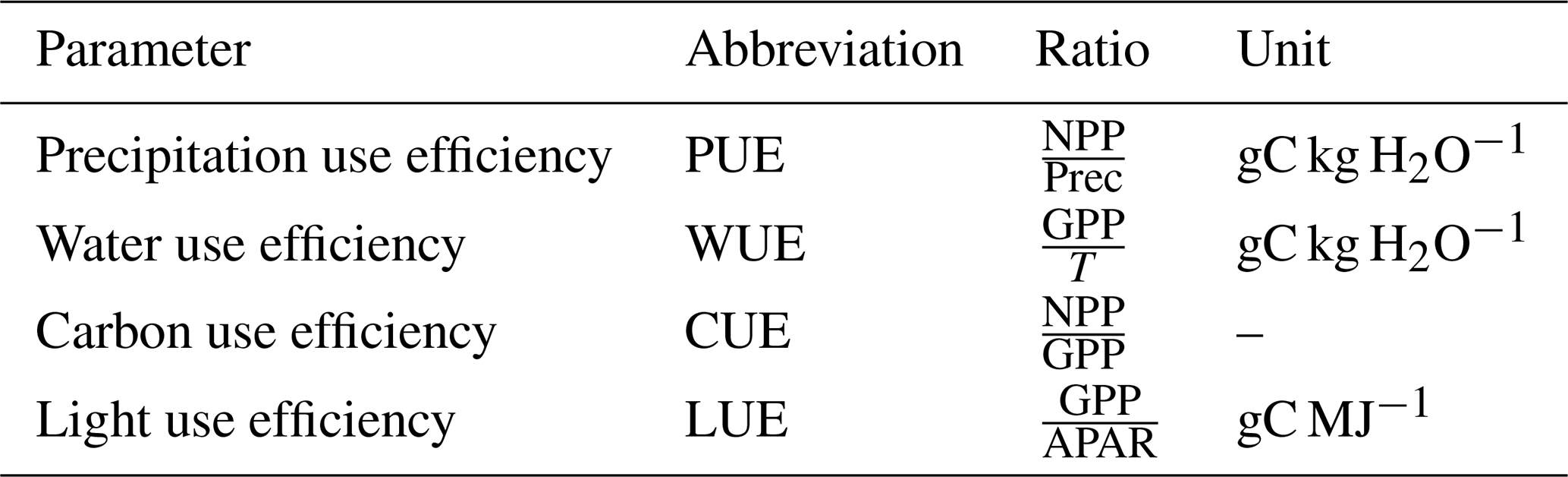
To assess the plausibility of simulated carbon-water relations we assess emerging spatial patterns of key functional parameters detailed in Table 3.

Table 3 Carbon-water cycle metrics used in this study, with abbreviations, definitions, and units.

3 Results and discussions

3.1 Model evaluation

3.1.1 Validation with independent test set

In this section, we evaluate the performance of H2CM in reproducing the monthly, MSC, and monthly anomalies of GPP and NEE across the testing set that was not exposed to the model during training (Fig. A1).

H2CM nearly perfectly reproduces the monthly and seasonal patterns of both GPP and NEE, with a Pearson's correlation coefficient (r) close to 1 (Figs. 3 and B1–B3). The monthly anomaly of GPP and NEE (based on OCO-2 data) has a Pearson's r of approximately 0.7 (mean across members), while the monthly anomaly of NEE based on CarboScope data has a Pearson's r of approximately 0.5. Uncertainties in the inversions of NEE monthly anomaly when locating in space and time also contribute to lowered performance metrics, as some of the variance in the inversions is noise, not signal.

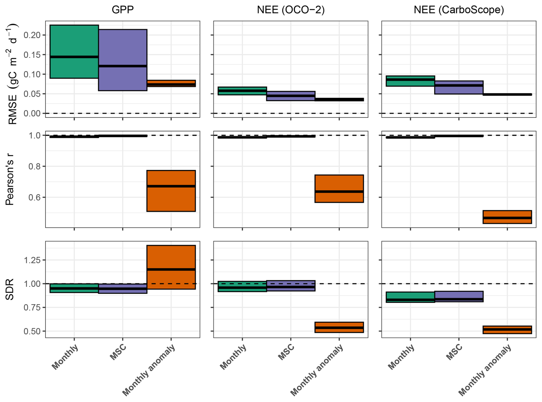
Figure 3 Model performance for carbon fluxes based on the spatial average over testing-set grid cells. Cross bars represent the minimum and maximum errors across the 10 cross-validation folds, and the central lines indicate the mean error. Rows correspond to performance metrics, and columns represent model constraints. RMSE denotes root mean squared error, and SDR is the standard deviation ratio (the ratio between predicted and observed standard deviation). Horizontal dashed lines denote ideal metric values, with R² and SDR equal to 1 and RMSE equal to 0.

The SDR for the monthly and seasonal patterns of GPP and NEE is close to 1, indicating the model's strong capability in accurately reproducing these patterns. The SDR for GPP monthly anomaly is greater than one, suggesting an overestimation of GPP monthly anomaly compared to FLUXCOM-X-BASE. This outcome is expected, as we do not explicitly constrain GPP monthly anomaly, and FLUXCOM-X-BASE is known to underestimate the GPP interannual variance (Nelson et al., 2024). Conversely, H2CM underestimates NEE monthly anomaly in both short-term (OCO-2) and long-term (CarboScope) contexts, as indicated by a low SDR value.

In terms of RMSE, H2CM tends to exhibit higher errors for monthly and seasonal data compared to monthly anomalies. This elevated RMSE primarily reflects the large magnitude of the seasonal cycle, such that even relatively small absolute deviations lead to substantial RMSE values. Despite this, the near-unity Pearson's r and SDR indicate that the phase and relative amplitude of the seasonal cycle are well captured. In contrast, the monthly anomalies exclude the dominant seasonal component, resulting in smaller RMSE due to their reduced variance, but typically lower correlations because only irregular year-to-year variations remain.

Globally, H2CM reproduces GPP patterns from FLUXCOM-X-BASE with RMSEs of 0.1, 0.09, and 0.05 gC m⁻² d⁻¹ for monthly data, mean seasonal cycles (MSC), and monthly anomalies, respectively. For NEE from OCO-2 satellite inversions, RMSEs are 0.04, 0.03, and 0.02 gC m⁻² d⁻¹ for the same categories. Compared to CarboScope in-situ inversions, H2CM yields RMSEs of 0.07, 0.06, and 0.03 gC m⁻² d⁻¹. Bias is negligible (close to 0) for GPP and NEE (OCO-2), and for NEE (CarboScope) is 0.01 gC m⁻² d⁻¹ for monthly and MSC data, and zero for monthly anomalies (Table B1).

Note that, although the results discussed here are based on the spatial-only cross-validation setup, Appendix C demonstrates that the model also generalizes well to unseen years, at least over short-term future periods. For example, when testing our model on unseen years for monthly GPP and NEE values, Pearson's r is close to 1 for GPP and 0.96 for NEE. These results hold for both the spatial split (original model) and spatio-temporal split experiments, with very similar ranges across cross-validation folds (Fig. C1).

Model performance on water cycle-related data constraints is presented in Appendix B. We do not delve into the details here, as the performance is qualitatively similar to that of H2MV, which has been thoroughly discussed in Baghirov et al. (2025).

3.1.2 Global patterns

3.1.3 Gross and net carbon fluxes

In this section, we evaluate H2CM's performance in terms of learned global mean spatial patterns of GPP and NEE. We compare H2CM's estimations to the data constraints provided by FLUXCOM-X-BASE and OCO-2 satellite inversions, as well as to the estimations from TRENDY.

FLUXCOM-X-BASE, H2CM, and TRENDY show very similar spatial patterns of mean GPP with largest values in wet tropical regions such as South America, Central Africa, and Southeast Asia (Fig. 4a). While mean annual GPP from H2CM and FLUXCOM-X-BASE are nearly identical, TRENDY tends to show somewhat larger GPP in central South America, central Africa, and Southeast Asia, while lower GPP across much of the Northern Hemisphere (Fig. B10a). H2CM reproduces the spatial patterns of mean NEE from the OCO-2 MIP, whereas TRENDY's estimations show little spatial gradients (Figs. 4b and B10b). Specifically, both H2CM and OCO-2 inversions suggest the largest carbon sources in northeastern South America, tropical Asia, and in the Savannah belt south of the Sahara in Africa. In contrast, the eastern parts of North America and Europe, the southwest of South America, areas south of the Equator in Africa, and the eastern parts of China appear as carbon sinks in the period 2015–2019.

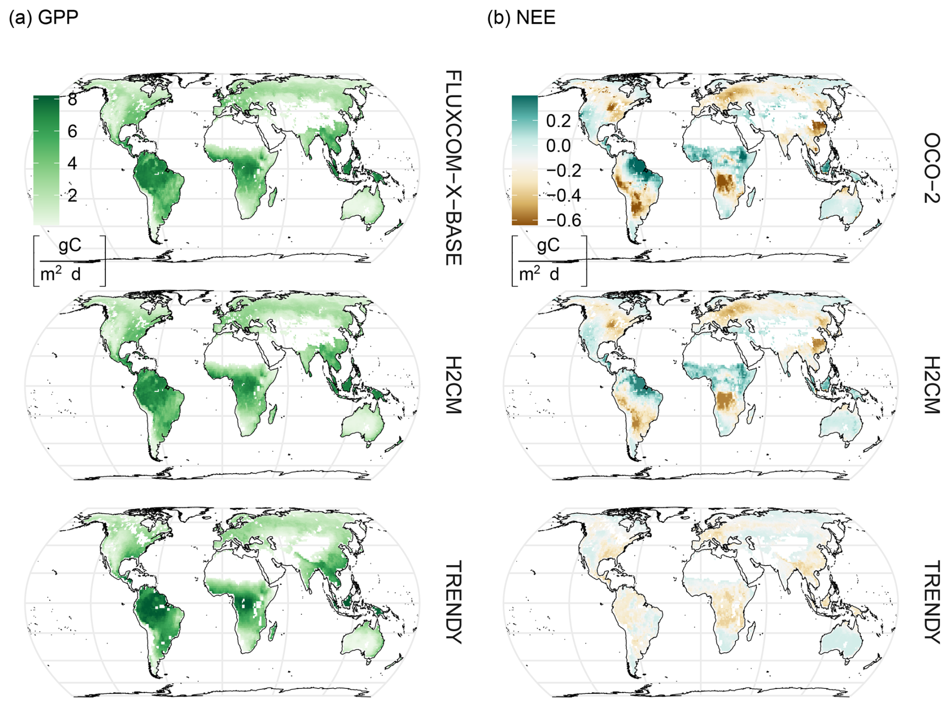
Figure 4 Comparison of predicted versus target global GPP and NEE against TRENDY estimates. Maps show the median predictions across members: H2CM (10-fold cross-validation, with members corresponding to folds), OCO-2 (inversion ensemble members), and TRENDY (individual process-based models). Column (a) shows GPP, while column (b) shows NEE. Mean annual averages are calculated over 2001–2019 for GPP and 2015–2019 for NEE.

3.1.4 Global spatial patterns of functional diagnostics

In this section, we qualitatively evaluate emerging global patterns in H2CM, focusing on key indicators such as precipitation, water, carbon, and light-use efficiency. These ratios, calculated based on mean annual values, help to diagnose and understand water–carbon cycle dynamics and coupling. Thus, this serves as credibility checks and a qualitative functional evaluation against patterns from existing studies in the literature.

H2CM estimates largest PUE values for high latitudes, particularly in regions such as western Canada, parts of Europe, and the Eurasian boreal regions (Fig. 5a). These findings strongly align with the results reported by Chen et al. (2020) that estimated rain use efficiency based on a light use efficiency model forced by satellite data, both in terms of spatial patterns and the magnitude of the estimations. Additionally, another study by Liu et al. (2024b) employed a regression model based on meteorology and remote sensing, to estimate rain use efficiency, specifically focusing on Australia. Although they used GPP to estimate rain use efficiency instead of NPP as we did, their findings for Australia are also very consistent with our model's estimates for the region such as reduced PUE in Australia's interior. Overall, H2CM estimates low PUE in very wet and very dry regions, indicating that PUE peaks at intermediate moisture conditions. In dry areas, the low PUE pattern can be attributed to lower vegetation growth rates (Paruelo et al., 1999), enhanced losses by evaporation (lower $T/\mathrm{ET}$, Nelson et al., 2024), or water losses through runoff after rare but intense rainfall. In wet regions, a large fraction of precipitation is lost to runoff, and other factors such as light and nutrients may limit photosynthesis, which also can also cause a decline of PUE (Paruelo et al., 1999; Huxman et al., 2004). We expect that PUE is very well constrained in H2CM because precipitation is a model input, and NPP is well constrained by data constraints on GPP and CUE.

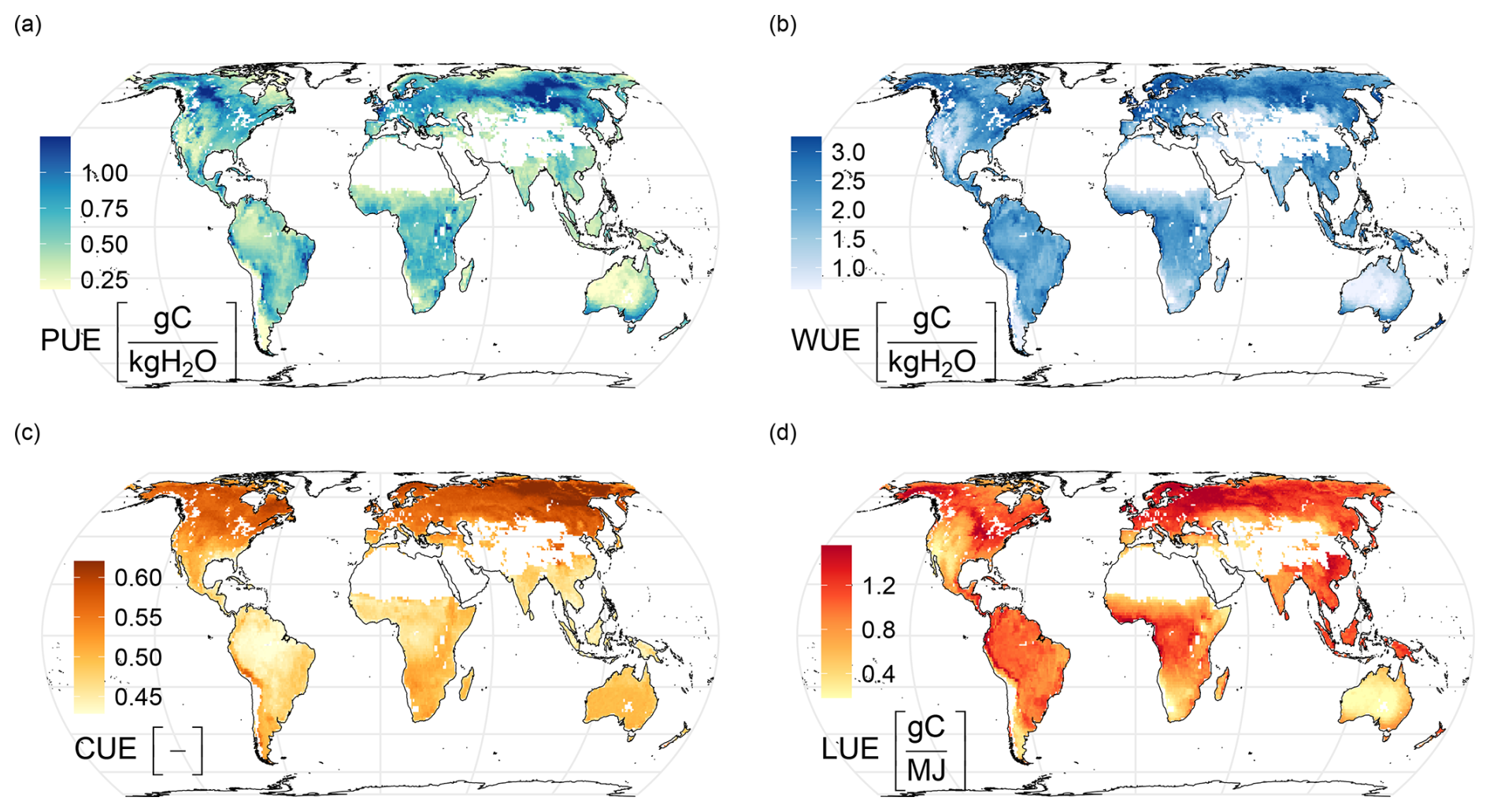
Figure 5 Emerging global patterns in H2CM: (a) Precipitation Use Efficiency ($\mathrm{PUE}=\mathrm{NPP}/\mathrm{Prec}$), (b) Water Use Efficiency ($\mathrm{WUE}=\mathrm{GPP}/T$), (c) Carbon Use Efficiency ($\mathrm{CUE}=\mathrm{NPP}/\mathrm{GPP}$), and (d) Light Use Efficiency ($\mathrm{LUE}=\mathrm{GPP}/\mathrm{APAR}$). The maps represent the median across 10 cross-validation folds. The mean annual average is calculated over the years 2001–2019.

H2CM estimates high WUE in regions such as northern North America (specifically Alaska and Canada), Northern Europe, the Eurasian boreal regions, certain areas in South America, Central Africa, the southernmost parts of Australia, and New Zealand (Fig. 5b). In contrast, H2CM predicts lower WUE for most arid regions. Low WUE estimations for arid regions is consistent with theory and observations predicting declining WUE with increasing VPD (Boese et al., 2019; Li et al., 2023; Medlyn et al., 2017, 2011; Katul et al., 2009). The attenuated WUE in tropical forests might be related to larger costs of transporting water through tall trees (Prentice et al., 2013). Our study defines WUE with respect to transpiration, while empirical studies often define it as a function of total evapotranspiration. This can lead to significant differences due to spatial variations of transpiration versus evapotranspiration (Lawrence et al., 2007; Wei et al., 2017b). However, Ito and Inatomi (2012) provides global WUE estimations as a function of GPP and transpiration based on process-based model simulations, which align well with H2CM's WUE estimations in terms of both spatial patterns and magnitudes. H2CM's WUE is constrained by GPP and ET data, while mainly fAPAR (also constrained by observations) and the respective process formulations constrain the partitioning of ET into transpiration and evaporation components.

H2CM generally estimates higher CUE values in higher latitudes and lower CUE values in most of the Southern Hemisphere (Fig. 5c). The range of these estimations is relatively narrow, approximately between 0.45 and 0.6, indicating that roughly 45 %–60 % of GPP is converted into net biomass. The patterns reflect the general expectation that the fraction of autotrophic respiration increases with temperature and biomass. This is expected because we have constrained the spatial pattern of mean annual CUE to align with predictions from the TRENDY ensemble of process models. Other studies have consistently reported similar findings in terms of magnitude and spatial patterns (He et al., 2018; Konings et al., 2019; Liu et al., 2019; Tao et al., 2023; Wang et al., 2022; Zhang et al., 2013).

H2CM estimates high effective LUE for regions such as the northwest parts of North America, the eastern states of Canada and the United States, Europe, the Eurasian boreal regions, South America, Central Africa, and Southeast Asia (Fig. 5d). Low LUE for dry regions are expected due to increased water limitations. A study by Liu et al. (202a), using FLUXNET site data and satellite-derived proxies, found results closely matching ours, particularly in spatial patterns. Similarly, Wei et al. (2017a) used random forest to estimate LUE based on flux tower data, aligning mostly with our estimations, though they report lower LUE values for the northwest part of North America and the Eurasian boreal regions.

3.2 Estimated seasonality of carbon fluxes across major regions

In this section, we assess the estimated seasonality of NEE, GPP, and TER as predicted by H2CM. Conceptually, H2CM is intended to be a bridge between purely data-driven approaches and purely process-based models. Therefore, we compare our estimations with both a pure data-driven model (FLUXCOM-X-BASE, Nelson et al., 2024) and state-of-the-art process-based models (TRENDY, Sitch et al., 2024). Our evaluation focuses on global and four major TransCom regions covering different climates: Eurasian Boreal, North American Temperate, South American Tropical, and Southern Africa (Fig. E1).

Overall, H2CM outperforms both FLUXCOM-X-BASE (in terms of NEE) and TRENDY (in terms of NEE and GPP) globally and across all regions, as measured by RMSE and R² (Fig. 6). H2CM, FLUXCOM-X-BASE, and TRENDY median all accurately capture most of the seasonal variation in global NEE and for the Eurasian Boreal region. However, the range among different TRENDY models is very large, and the ensemble median underestimates the peak of net carbon uptake in summer, apparently due to an underestimation of GPP (Fig. 6).

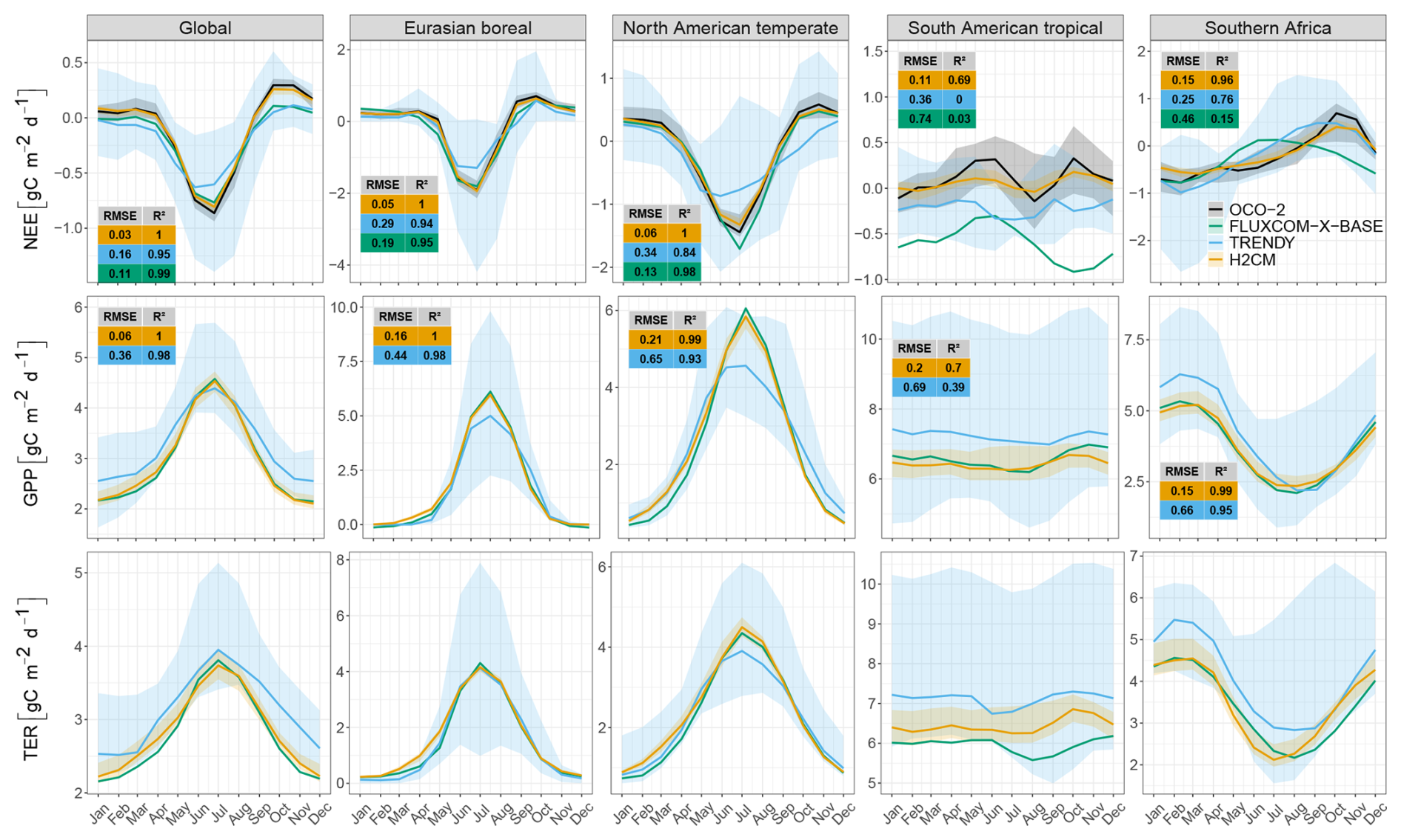
Figure 6 Predicted seasonality of carbon fluxes compared with data constraints, FLUXCOM-X-BASE, and TRENDY across four major Transcom regions. Shaded areas represent the range across model members (or 10 CV folds in H2CM), with lines indicating the median. Each column corresponds to a different region, and each row represents a distinct carbon flux. Subplots for NEE and GPP include tables with metrics for each region. NEE comparisons involve H2CM, FLUXCOM-X-BASE, and TRENDY against OCO-2 inversions, while GPP comparisons involve H2CM and TRENDY with FLUXCOM-X-BASE. Metrics for TER are omitted due to the absence of direct data constraints. Note varying y-axis scales for different regions.

For the North American Temperate region, both H2CM and FLUXCOM-X-BASE effectively capture most of the seasonal variation in NEE, with R² values of 1 and 0.98, respectively. In terms of TER, there is good agreement across all approaches (Fig. 6). Similar as for the Eurasian boreal region, TRENDY median underestimates the net carbon uptake peak in summer peak of NEE, and exhibits a slight phase shift of NEE seasonality. This issue seems attributable to TRENDY's GPP estimations, where similar problems are observed (underestimation of the peak and slight shift).

In the South American Tropical region, only H2CM captures 69 % of the subtle seasonal variation in NEE, which shows a seasonal cycle characterized by a double peak of net carbon release. FLUXCOM-X-BASE captures the first carbon release peak qualitatively but not the second, while TRENDY's seasonality seems unrelated to the OCO-2 inversion estimates. Interestingly, the seasonality of GPP is similar between H2CM, FLUXCOM, and TRENDY, while seasonality of TER deviate across modeling approaches. The discrepancy of FLUXCOM and TRENDY with respect to NEE variations of H2CM is dominated by TER, as H2CM estimates a positive TER peak in October, which TRENDY and FLUXCOM-X-BASE do not. The peak of net carbon uptake suggested by OCO-2 inversions does not coincide with the GPP peak, which is qualitatively reproduced by H2CM. One possible explanation for the poor NEE estimations in the South American Tropical region is the potential omission of certain processes in the models. Given the role of respiration in shaping net carbon release patterns in the wet tropics and the apparent discrepancies related to TER among models, it seems that wetness effects on respiration remain to be a modelling issue. H2CM's neural network component seems effective to compensate for this to some extent by learning responses from the observational constraints.

In Southern Africa, H2CM explains most of the variation in NEE (based on OCO-2 MIP) with an R² of 0.96. TRENDY reasonably reproduces the patterns with an R² of 0.76, while FLUXCOM-X-BASE performs poorly with an R² of 0.16. Also in this subtropical dry region, NEE seasonality and discrepancies among models seem related to respiration as both H2CM and TRENDY capture most of the variation in GPP in terms of R² (Fig. 6). H2CM accurately reproduces the prominent peak of net carbon release at the end of the year, whereas TRENDY captures it poorly, showing a slight shift in the peak estimation, and FLUXCOM-X-BASE completely misses it (Fig. 6). Several studies have highlighted the challenges of correctly capturing NEE seasonality in dry regions (Jung et al., 2020; Lee et al., 2025; Metz et al., 2025; Nelson et al., 2024; Bodesheim et al., 2018). The carbon release peak in Southern Africa was attributed to the rapid stimulation of microbial respiration due to re-wetting when transitioning from the dry to the rainy season (Metz et al., 2023, 2025). Also for dry subtropical regions FLUXCOM-X-BASE and TRENDY models struggle to accurately represent the differential responses of photosynthesis and respiration processes to water effects. These carbon-water interactions lead to complex seasonal variations of NEE, which are characterized by carbon release peaks in contrast to boreal and temperate regions dominated by a GPP driven carbon uptake peak. In the next section, we further diagnose the origin of the carbon release peak in Southern Africa by H2CM.

3.3 Net carbon release peak in Southern Africa

In this section, we focus on the drylands of Southern Africa – a region with large contribution to global NEE interannual variability but where FLUXCOM-X-BASE and TRENDY struggle to reproduce even seasonal dynamics. We analyze how H2CM represents the patterns and processes governing NEE seasonality in this region and show that our hybrid modeling approach provides insight into these complex dynamics.

To infer which regions contribute most to the end-of-year net carbon release peak in Southern Africa, we plotted the NEE difference between December and August (Fig. 7a). Interestingly, the largest amplitude occurs in the sub-humid region covering the Miombo woodlands, and not in the drier southern part of Africa. Similarly, Metz et al. (2025) inferred that the more northern regions of Southern Africa contribute most to the peak based on an atmospheric inversion using GOSAT data, while those did not permit a more detailed spatial assessment.

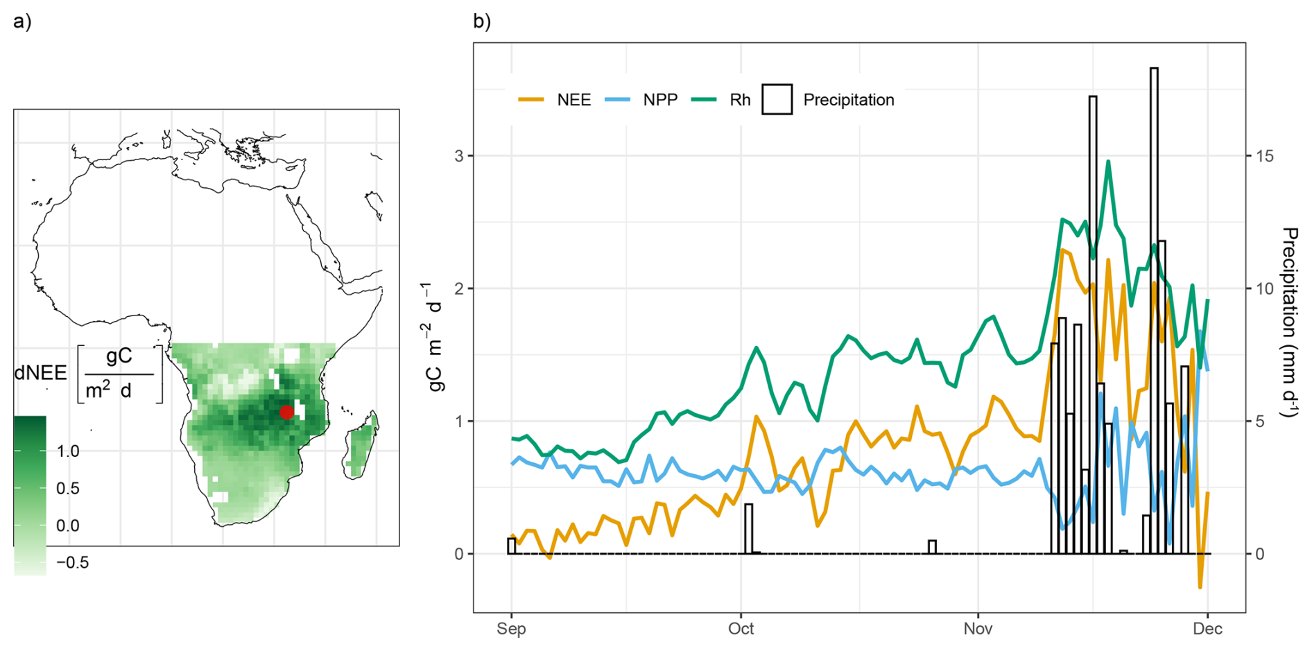
Figure 7 (a) The difference in NEE between the peak month (December) and the onset of the gradual increase (August). The black point on the map indicates the specific grid cell location from which the time-series data is derived. (b) Response of CO₂ fluxes to rainfall in Southern Africa. The left y axis represents CO₂ flux values, while the right y axis corresponds to precipitation values. The time-series is based on daily flux predictions from September through December for 2006 and median across 10-CV folds.

To better understand the simulated carbon dynamics by H2CM, we plot daily variations of NEE, NPP, and heterotrophic respiration for a grid cell in the center of this region (Fig. 7a). The NEE variations from August to December are characterized by a gradual increase until about November, driven by a concomitant rise in Rh (Fig. 7a). With the onset of the rain, both Rh and NEE exhibit sharp increases. This phenomenon aligns with the “Birch effect” (Birch, 1964; Jarvis et al., 2007), where re-wetting causes a respiration pulse. Recent studies based on atmospheric inversions using GOSAT data have found that this effect shapes NEE variations in dry areas such as Australia (Metz et al., 2023), Southern Africa (Metz et al., 2025) and dry regions of South America (Vardag et al., 2025).

Interestingly, at this location, we also observe that NPP declines when it rains, which further amplifies the NEE response. This suggests that in H2CM, the region's GPP gets limited by light rather than water, due to reduced radiation from cloudiness. In fact, previous studies indicate that the Miombo forests remain green throughout the dry season (Küçük et al., 2022), likely due to water access through deep rooting (Stocker et al., 2023). Our findings based on H2CM suggest that light limitation of photosynthesis in the Miombo contributes to the end-of-season NEE peak in Southern Africa, in addition to the previously known re-wetting driven respiration response.

This example highlights H2CM's ability to capture and explain complex carbon cycle phenomena. It suggests that H2CM learned plausible carbon flux responses to high-frequency (daily) variations in environmental conditions, even though only low-frequency (monthly) data constraints were used during training.

3.4 Discussion of the H2CM approach

3.4.1 Scope and strength

H2CM is a process-aware hybrid framework that integrates machine learning with simplified process-based formulations, and can be positioned within the broader family of model–data integration strategies that aim to combine physics with machine learning. This family includes approaches such as physics-informed neural networks (Tartakovsky et al., 2020; Wang et al., 2020; Raissi et al., 2019), physics-guided machine learning (pgml, Pawar et al., 2021; Karpatne et al., 2017), and differentiable modeling (Shen et al., 2023). Rather than reproducing the detailed parameterizations used in comprehensive land-surface models, H2CM employs conceptual process formulations to maintain interpretability and ensure parameter identifiability under the available observational constraints.

The primary objective of H2CM is to deliver a consistent, observation-constrained “reanalysis” of coupled carbon–water states and fluxes over recent decades by fusing diverse data streams within a process-informed ML architecture. H2CM is not intended to replace land surface models coupled into Earth system models, nor to provide long-term projections; such applications would require more complete representations of processes and feedback. Instead, H2CM can be perceived as a bridge between empirical and process-based modeling which enables a coherent interpretation of only partially observed coupled carbon–water cycle variability and interactions. H2CM is a global model in the sense that it is applied consistently across grid cells covering the global land surface, while it remains local as it does not simulate lateral processes among grid cells. Although the domain and grid are, in principle, arbitrary, the present design is tailored to comparatively coarse grid cells for improved consistency with spatially coarse observational constraints like TWS from GRACE or NEE inversions.

H2CM advances the field by combining previous approaches – such as fully data-driven models like FLUXCOM(-X-BASE) (Jung et al., 2019, Jung et al. (2020), Nelson et al. (2024)) and fully process-based models like TRENDY (Sitch et al., 2015, Sitch et al. (2024)) – by aiming at combining their strengths: it learns directly from global observations through its machine learning component, while respecting conceptual process understanding and mass balance. Relative to process-based TRENDY models, which rely on numerous parameterizations yet struggle with regional and climate-specific patterns in observation-based carbon fluxes, H2CM better captures key spatial–temporal features in observations (Fig. 6). Likewise, compared with fully data-driven FLUXCOM approaches that depend primarily on site-level eddy covariance data and can underperform in tropical and subtropical regions with sparse coverage, H2CM leverages complementary data streams and process-aware structure to improve generalization (Fig. 6).

Both, the rich information provided by complementary Earth Observations to H2CM, and the flexibility of machine learning to exploit these, contribute to the good performances of the model. Clearly, a key factor for the improved performance of H2CM compared to FLUXCOM in capturing NEE variations inferred from atmospheric inversions is the integration of this data constraint in the hybrid modeling approach. While this might also explain H2CM's improved performance compared to TRENDY, the machine learning component used to parameterize the conceptual process equations seems to contribute to the success significantly. A useful point of reference is the model-data-integration approach by Lee et al. (2025), which shares a similar model structure of conceptual process equations of carbon and water cycles, and nearly identical observational constraints. The key difference is the representation of parameters in process equations: the study by Lee et al. (2025) assumes globally constant parameters, whereas H2CM uses neural networks to predict parameters that vary spatially and/or temporally. Overall, both approaches, being strongly data-constrained, capture large-scale patterns well. However, H2CM achieves higher performance, in particular in dry and wet tropical regions with partly complex linkages of carbon and water cycles. This illustrates the added value of the adaptive machine learning module in H2CM for better model performance. Taken together, H2CM's skill emerges from the synergy of conceptual process formulations, diverse observational constraints, and adaptive parameterization through machine learning.

3.4.2 Uncertainties and limitations

H2CM heavily depends on data-driven learning, incorporating both meteorological forcings and data constraints. The primary constraints on the carbon cycle include GPP seasonality from FLUXCOM-X-BASE, NEE from OCO-2, and global NEE monthly anomalies from CarboScope. Each of these data sources is subject to uncertainties, which could propagate to H2CM. Accounting for data uncertainties explicitly in H2CM, e.g. based on a Bayesian approach, would be desireable conceptually. However, the lack of adequate and comparable quantitative information on data uncerainties across different data streams limits this approach in practice.

We tried to mitigate known issues of the observational constraints by making the loss function sensitive to the more robust patterns in the data, e.g. by using only the mean seasonal cycles of GPP by FLUXCOM-X-BASE due to known limitations for interannaul variability (Jung et al., 2020; Nelson et al., 2024). However, uncertainty of the GPP mean seasonal cycle of X-BASE remain for example in the region of tropical South America. Thus, potential biases in the seasonal cycle of FLUXCOM-X-BASE GPP likely propagate to H2CM, which could then also compromise simulations of respiration due to the concomitant data constraint on NEE.

To constrain H2CM's NEE estimations, we utilize an atmospheric inversion ensemble using in-situ and OCO-2 satellite-based column XCO₂ data. Despite significant efforts and advancements in XCO₂ retrievals from OCO-2, the preferential sampling of clear-sky conditions and remaining retrieval biases may affect inferred NEE variations (Connor et al., 2016; Kulawik et al., 2019a, b; Worden et al., 2017). Additional uncertainties from various methodological choices, particularly in atmospheric transport modeling, result in poorly constrained spatial inversion results (Yun et al., 2025; Zhang et al., 2022; Byrne et al., 2023). We used 1° OCO-2 MIP results to constrain NEE, which, despite the added value of extensive XCO₂ data, may be overly optimistic. Therefore, some discrepancies between H2CM-simulated and OCO-2 MIP-based NEE at 1° resolution (Fig. B10b) are due to this data constraint uncertainty. Since the issue of loose spatial constraints is even more pronounced for atmospheric inversions using only the sparse in-situ CO₂ network, we used only the spatial batch average as a data constraint from CarboScope.

Exploiting H2CM's explicit process interpretability for process understanding requires sufficiently strong observational constraints to overcome equifinality – i.e., different processes or pathways yielding similar outcomes when data are not informative enough. Examining the spread among 10 CV models trained on different cross-validation folds and with different random initializations indicates good qualitative robustness under varying training data (Baghirov et al., 2025). Nevertheless, the globally constant temperature sensitivity of respiration (Q₁₀) and the scalar for the relative CO₂ fertilization effect on GPP (${\mathit{\beta }}_{{\mathrm{CO}}_{\mathrm{2}}}$) show signs of non-identifiability. Across CV folds, the median Q₁₀ (unitless) is 1.25, with a range of 1.24–1.27, lower than literature values for heterotrophic/soil respiration (1.4–2; Zhou et al., 2009; Meyer et al., 2018; Niu et al., 2021). For ${\mathit{\beta }}_{{\mathrm{CO}}_{\mathrm{2}}}$ the median value learned across CV folds is 35.82 (% 100 ppm⁻¹). The range of values extends from 26.88 (% 100 ppm⁻¹) to 62.71 (% 100 ppm⁻¹), which exceeds observational estimates of roughly 14 % 100 ppm⁻¹–16% 100 ppm⁻¹ (Ainsworth and Rogers, 2007; Wang et al., 2020; Ueyama et al., 2020; Zhan et al., 2024). To probe this, we imposed informative priors on these global constants (Appendix D). Under these priors, H2CM recovered ${\mathit{\beta }}_{{\mathrm{CO}}_{\mathrm{2}}}=\mathrm{15}$ (% 100 ppm⁻¹) and Q₁₀=1.5 – matching the priors exactly – while other model results and performance remained qualitatively unchanged. These findings indicate that with the current data constraints, Q₁₀ and ${\mathit{\beta }}_{{\mathrm{CO}}_{\mathrm{2}}}$ are not fully identifiable, underscoring the value of stronger observational constraints and the incorporation of process knowledge (e.g., via priors or loss-function regularization) for decadal-scale assessments with H2CM.

Deviations of H2CM simulations from the data constraints such as for NEE in tropical South America (Fig. 6) are useful indications for missing information or issues in the data. This is because H2CM cannot fit the data constraints if (1) the relevant signals are not present in the model forcing data; or (2) the model's process formulations do not permit it, e.g. due to a missing process representation that cannot be captured by the flexibility of the machine learning component; or (3) because there is a conflict among different observational constraints that cannot be satisfied simultaneously given the process formulations.

While incorporating process understanding in H2CM also provides theoretical constraints that can help to regularize the NNs (Reichstein et al., 2019; Shen et al., 2023), a trade-off between model complexity and parameter identifiability is obvious. Thus the simple nature of process representations in H2CM is justified by the limited information content of the used observations to disentangle subprocesses, and by minimum requirements on interpretability. For example, we use net radiation as a single forcing term rather than separately prescribing shortwave and longwave components for simplicity as shortwave and net radiation are strongly correlated at daily time scale (Jung et al., 2024). Currently, H2CM lacks several important components of the land system, which are relevant for the coupled water and carbon cycles. For example, it does not yet explicitly model vegetation and soil carbon pools, as the current focus has been on spatial variations of carbon fluxes from sub-seasonal to interannual time scales. Furthermore, H2CM does not incorporate the effects of disturbances such as fire, or other drivers including land-use change. Note that dynamic vegetation changes are not explicitly represented in H2CM; however, temporal variations in fAPAR provide an implicit representation of phenological changes. There are emerging opportunities from the observational side which could support the integration of these components in H2CM in the future.

4 Conclusions

We introduced H2CM – a hybrid global carbon-water cycle model constrained by diverse observational data streams, which acts as a bridge between empirical and process-based modeling and enables a coherent interpretation of only partially observed coupled carbon–water cycle variability and interactions. H2CM integrates key hydrological data streams such as terrestrial water storage variations from GRACE, but also combines flux tower based bottom-up and atmospheric top-down data constraints of the carbon cycle. We demonstrated that H2CM successfully integrates the strengths of machine learning and process-based modelling, learning directly from observations while obeying to process understanding. H2CM reproduces major observed patterns of carbon flux variations and spatial patterns of functional carbon-water coupling properties. Our parallel evaluation of H2CM with the purely data-driven FLUXCOM and process-based TRENDY model ensemble further highlights the added value of our hybrid approach in modelling uncertain moisture effects on respiration, which shape NEE variations in dry and wet tropical regions significantly.

H2CM opens new avenues for studying the global carbon–water cycle and lays the groundwork for further developments toward a hybrid data-driven land–surface model. Advancing in this direction will require integrating the surface energy cycle, incorporating dynamic vegetation and explicit carbon pools, representing additional key processes and disturbances (e.g., permafrost, fire, and land use/management), and resolving sub-daily dynamics. These opportunities are forward-looking, while the grand challenge will be to achieve a robustly constrained model with causal functioning required to simulate conditions with no analogs in the contemporary observational era.

Appendix A: Cross validation

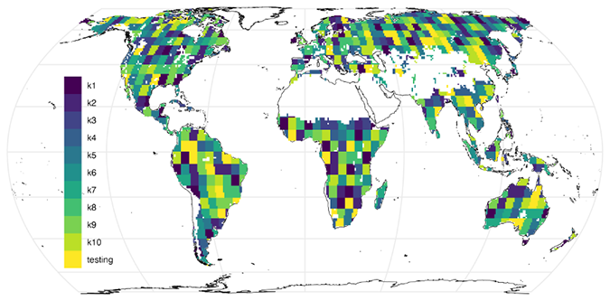
Figure A1 Validation sets for 10 different models and a fixed testing set. Note that, during training, each fold has a separate and unique validation set and all models were tested on the same testing set.

Appendix B: Model evaluation

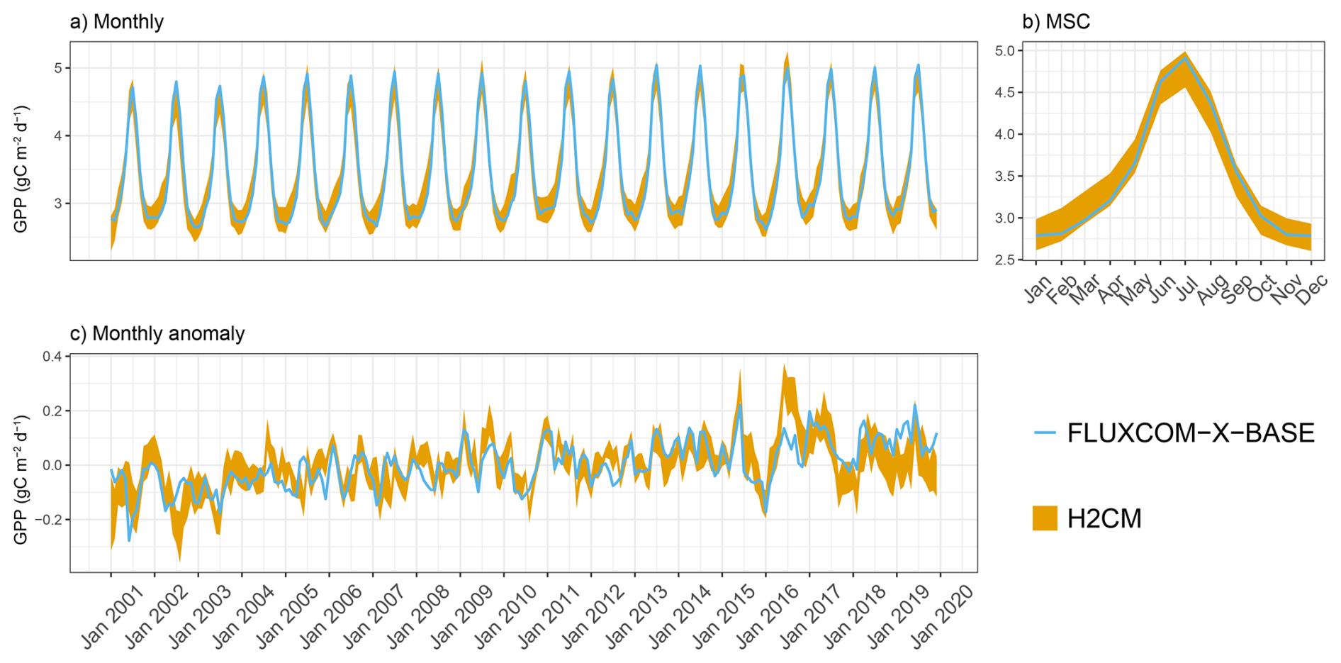
Figure B1 Predicted versus target GPP (FLUXCOM-X-BASE) over the testing set (spatial domain) across 10 CV folds: (a) monthly, (b) mean seasonal cycle over the entire period of data constraint and (c) monthly anomaly.

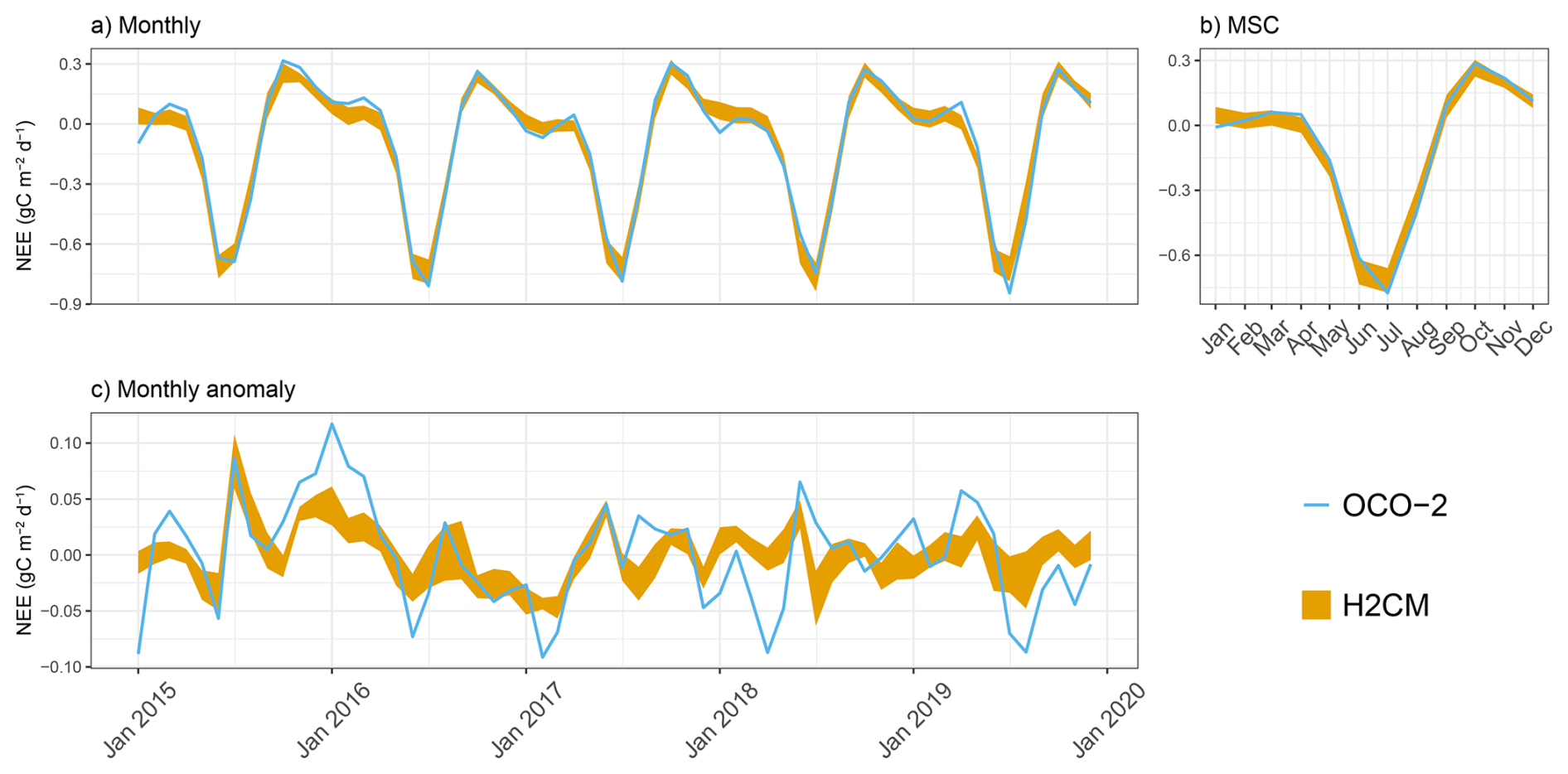
Figure B2 Predicted versus target NEE (OCO-2) over the testing set (spatial domain) across 10 CV folds: (a) monthly, (b) mean seasonal cycle over the entire period of data constraint and (c) monthly anomaly.

Figure B3 Predicted versus target NEE (CarboScope) over the testing set (spatial domain) across 10 CV folds: (a) monthly, (b) mean seasonal cycle over the entire period of data constraint and (c) monthly anomaly.

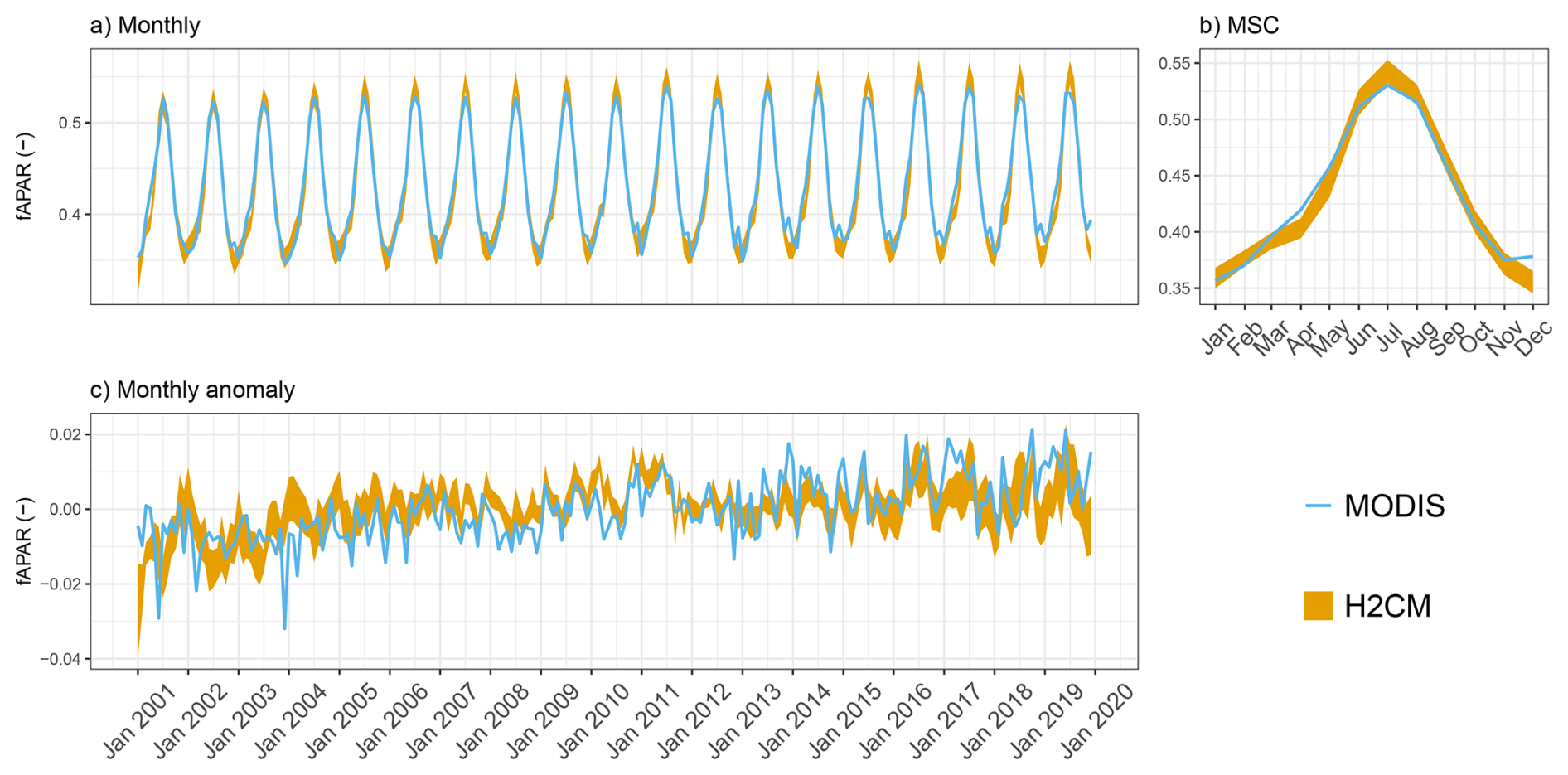
Figure B4 Predicted versus observed mean fAPAR over the testing set (spatial domain) across 10 CV folds: (a) monthly, (b) mean seasonal cycle over the entire period of data constraint and (c) monthly anomaly.

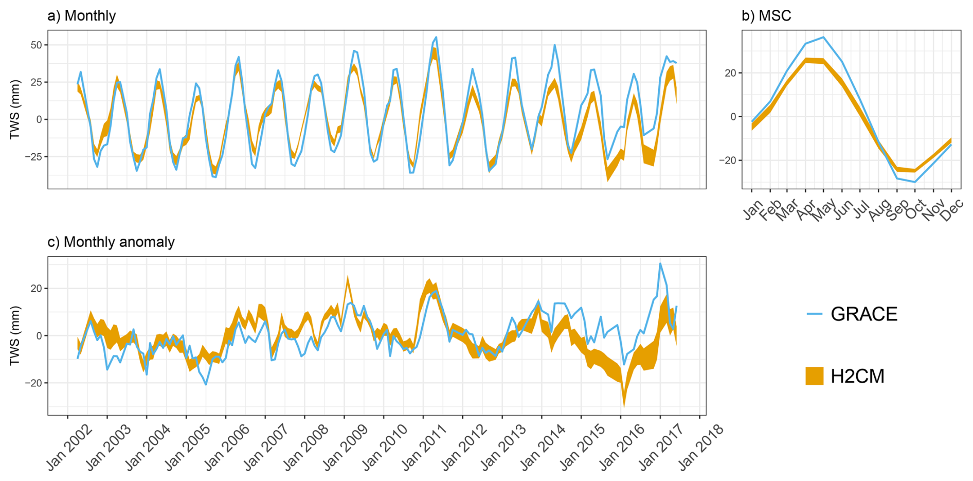
Figure B5 Predicted versus observed mean terrestrial water storage (TWS) (anomaly) over the testing set (spatial domain) across 10 CV folds: (a) monthly, (b) mean seasonal cycle over the entire period of data constraint and (c) monthly anomaly.

Figure B6 Predicted versus observed mean snow water equivalent (SWE) over the testing set (spatial domain) across 10 CV folds: (a) monthly, (b) mean seasonal cycle over the entire period of data constraint and (c) monthly anomaly.

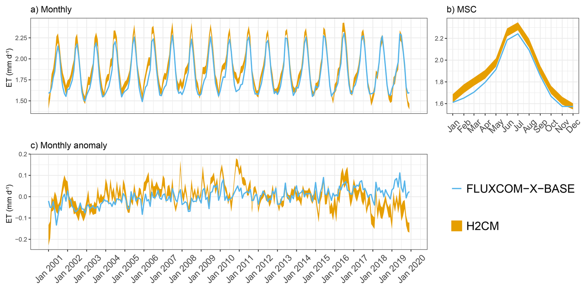
Figure B7 Predicted versus target mean ET over the testing set (spatial domain) across 10 CV folds: (a) monthly, (b) mean seasonal cycle over the entire period of data constraint and (c) monthly anomaly.

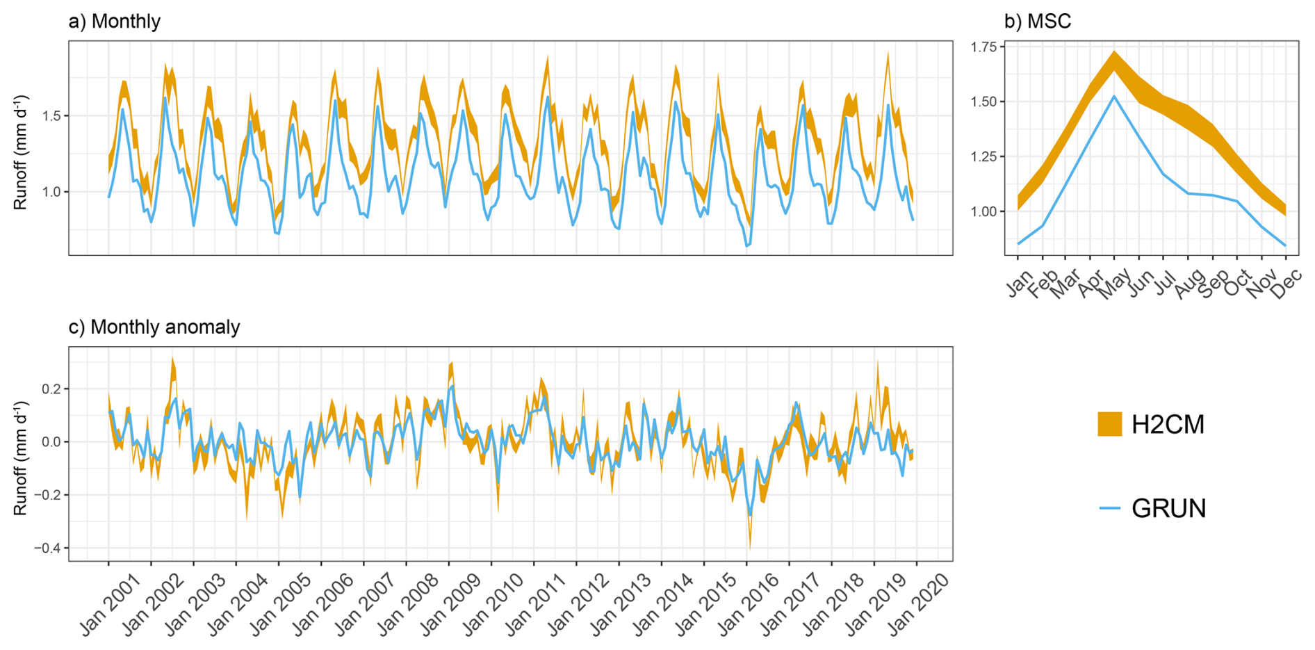
Figure B8 Predicted versus target mean runoff over the testing set (spatial domain) across 10 CV folds: (a) monthly, (b) mean seasonal cycle over the entire period of data constraint and (c) monthly anomaly.

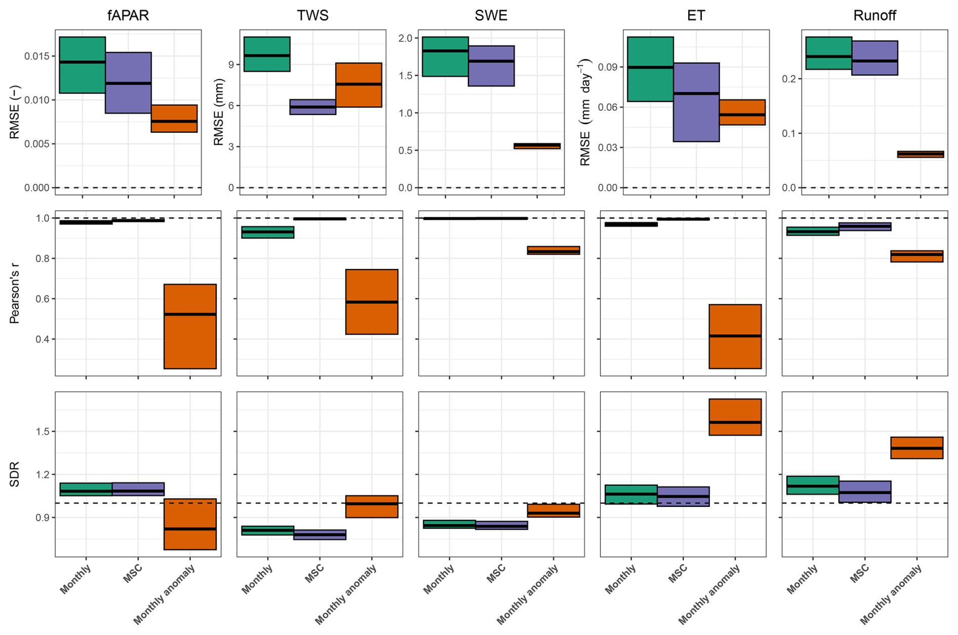
Figure B9 Model performance for vegetation, water storages and fluxes based on the spatial average over testing-set grid cells. Cross bars represent the minimum and maximum errors across the 10 cross-validation folds, and the central lines indicate the mean error. Rows correspond to performance metrics, and columns represent model constraints. RMSE denotes root mean squared error, and SDR is the standard deviation ratio (the ratio between predicted and observed standard deviation). Horizontal dashed lines denote ideal metric values, with R² and SDR equal to 1 and RMSE equal to 0.

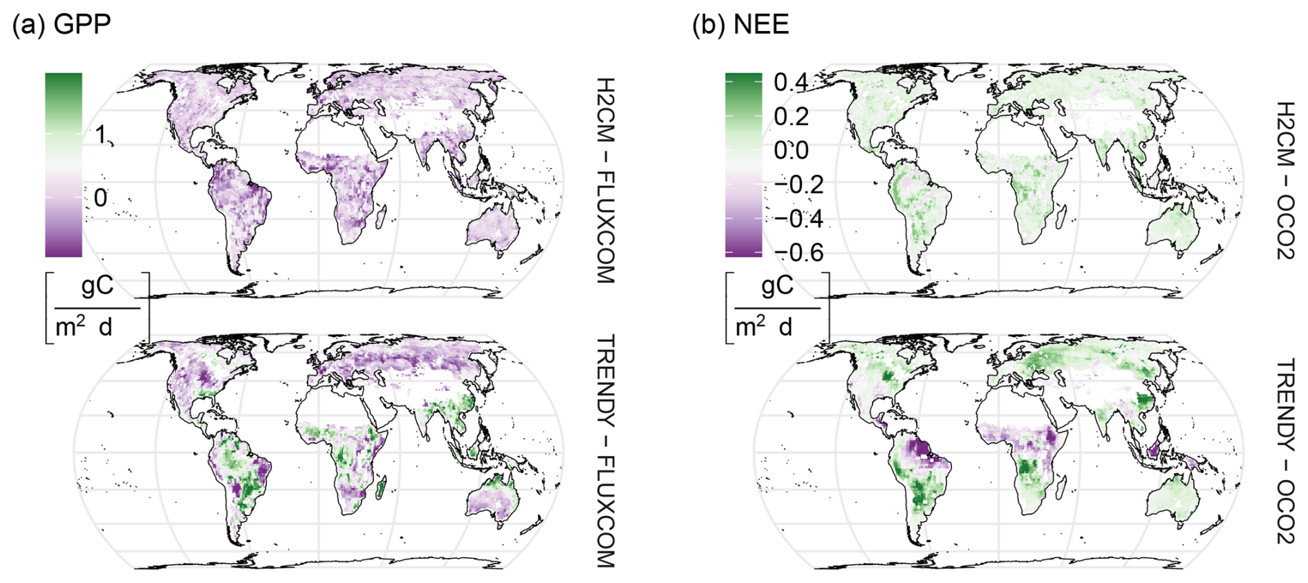
Figure B10 Spatial differences between modelled and target carbon fluxes for (a) gross primary production (GPP) and (b) net ecosystem exchange (NEE). The figure compares the median estimations from H2CM (10-fold cross-validation), OCO-2 (inversion ensemble), and TRENDY (process-based model ensemble). For GPP, H2CM and TRENDY are evaluated against FLUXCOM, averaged over 2001–2019; for NEE, both are evaluated against OCO-2 MIP, averaged over 2015–2019.

Table B1 Benchmarking metrics (RMSE and Bias) for modeled carbon fluxes against data constraints. Metrics are reported for gross primary productivity (GPP) and for net ecosystem exchange (NEE) benchmarked against OCO-2 and CarboScope inversion products. Each section – GPP, NEE (OCO-2), NEE (CarboScope) – summarizes results for Monthly, mean seasonal cycle (MSC), and Anomaly data. All metrics are based on globally averaged, area-weighted time series. Reported values represent the median across 10-fold cross-validation runs, with values in brackets indicating the minimum and maximum across folds.

Appendix C: Model generalization across space and time

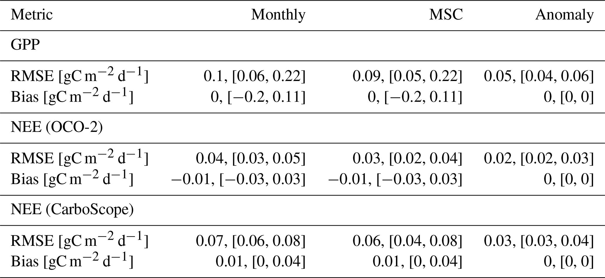
Figure C1 shows the performance comparison between spatially split and spatio-temporally split cross-validation folds using post-2017 time-series data. In the spatial split experiment, the model was trained on the complete 2001–2019 time series while holding out specific spatial grid cells for testing. In contrast, the spatio-temporal split experiment was trained on data from 2001–2017, with all data after 2017 withheld for spatio-temporal testing.

Overall, the results suggest that the model maintains consistent performance when evaluated on the two unseen years, demonstrating generalisability not only across space but also over time – at least when tested on short-term future periods. In the spatio-temporal split experiment, neither the testing grid cells nor the final two years (2018–2019) were included in model training or validation, ensuring a fully unseen temporal and spatial domain during testing.

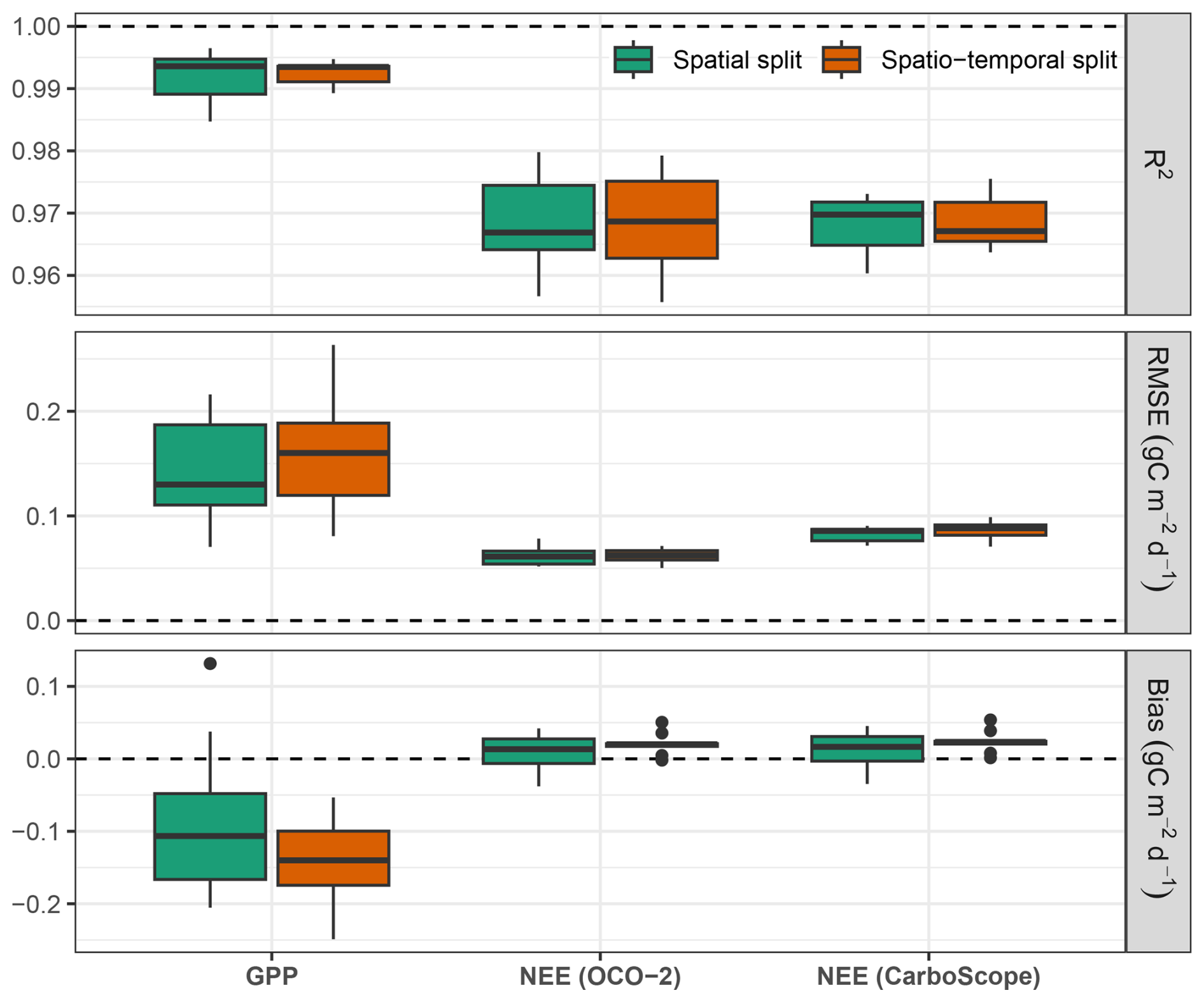
Figure C1 Model performance evaluated on the testing set comprising post-2017 time-series data, averaged over the testing grid cells. In the spatial split experiment, the model was trained on the full 2001–2019 dataset while holding out specific spatial grids for testing. In contrast, the spatio-temporal split experiment was trained only on data from 2001–2017, ensuring that no post-2017 information was included during training. Boxplots illustrate the distribution of errors across 10 cross-validation folds. Horizontal dashed lines denote ideal metric values, with bias and RMSE equal to 0 and R² equal to 1.

Appendix D: Regularization on global constants

To incorporate prior knowledge into H2CM's estimation of its global parameters, we add the following penalty term to the loss:

$$\begin{array}{}\text{(D1)}& l_{\mathrm{p}}={\displaystyle \frac{(\widehat{\mathit{\theta }}-\mathit{\theta }{)}^{\mathrm{2}}}{{\mathit{\sigma }}_{\mathit{\theta }}^{\mathrm{2}}}}.\end{array}$$

Here, $\widehat{\mathit{\theta }}$ is the estimated global constant, θ is the target (reference) value based on prior knowledge, and σ_θ controls the strength of the regularization (analogous to the expected uncertainty in $\widehat{\mathit{\theta }}$).

Note that formulation does not represent a Bayesian update but instead serves as a constraint that discourages large deviations from previously known reasonable values.

In our experiments:

• For ${\mathit{\beta }}_{{\mathrm{CO}}_{\mathrm{2}}}$, we set

  $$\begin{array}{ll}{\displaystyle }& {\displaystyle }\mathit{\theta }=\mathrm{15}\mathit{\%}\mathrm{100}{\mathrm{ppm}}^{-\mathrm{1}},\\ {\displaystyle }& {\displaystyle }{\mathit{\sigma }}_{\mathit{\theta }}=\mathrm{5}\mathit{\%}\mathrm{100}{\mathrm{ppm}}^{-\mathrm{1}}.\end{array}$$

• For the temperature sensitivity, Q₁₀, we use

  $$\begin{array}{ll}{\displaystyle }& {\displaystyle }\mathit{\theta }=\mathrm{1.5},\\ {\displaystyle }& {\displaystyle }{\mathit{\sigma }}_{\mathit{\theta }}=\mathrm{0.3}.\end{array}$$

Under this setup, H2CM estimates

$$\begin{array}{ll}{\displaystyle }& {\displaystyle }{\mathit{\beta }}_{{\mathrm{CO}}_{\mathrm{2}}}=\mathrm{15}\mathit{\%}\mathrm{100}{\mathrm{ppm}}^{-\mathrm{1}},\\ {\displaystyle }& {\displaystyle }{Q}_{\mathrm{10}}=\mathrm{1.5},\end{array}$$

which coincide with their reference values. We note that the observed agreement between estimates and reference values may partly be driven by the strong influence of the prior (regularization) term in the loss function, which constrains the model and reduces its ability to deviate from the reference. At the same time, this behavior also reflects underdetermination: the observational data do not provide sufficient information to move the parameters substantially away from the prior. Without additional data or process constraints, H2CM's global constants remain underdetermined by the current observations and knowledge alone; therefore, including prior terms in the loss function is currently important.

Appendix E: Major regions studied

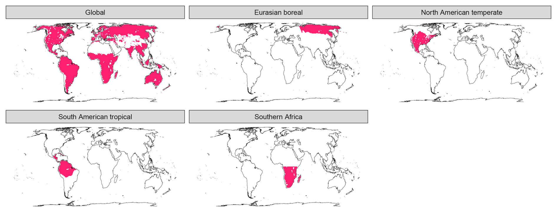
Figure E1 Major Transport and Climate Monitoring (TransCom, Baker et al., 2006) regions studied in this study.