Towards high-fidelity simulations of coastal submesoscale baroclinic instabilities with MPAS-O (vE3SM3.0.0) – Part 1: Idealized experiments

Rapid advances in computational power over the past decade have enabled global, kilometer-scale simulations that realistically represent open-ocean submesoscale dynamics. However, the ability of global ocean models to represent coastal submesoscale dynamics – where flows are more heterogeneous and strongly shaped by coastlines, bathymetry, and buoyancy inputs – remains largely unexplored. This study is the first of two companion papers comparing coastal submesoscale processes representation in two models with very different numerical approaches: MPAS-O, an unstructured grid global ocean model, and ROMS, a structured grid regional model. This study is the first idealized evaluation of MPAS-O’s representation of coastal submesoscale dynamics using observed conditions in the Mississippi-Atchafalaya (M-A) River plume as a template for initial conditions, with the previously validated ROMS model serving as a benchmark. An important motivation for this study is to examine the suitability of models designed for global ocean simulations in reproducing energetic coastal flows. We compare statistical metrics based on flow invariants – total strain, relative vorticity, and divergence – as well as velocity gradients in frontal coordinates, across horizontal resolutions ranging from 10 km to 100 m within an idealized model domain. We find that the representation of submesoscale baroclinic instabilities is highly similar across all resolutions such that the impact of model choice is smaller than the choice of spatial grid resolution. We also compare numerical and physical mixing between models using online diagnostics based on discrete variance decay. We find that ROMS generally has more numerical mixing and less physical mixing than MPAS-O across all resolutions. Trends in numerical mixing likely arise from MPAS-O's flux-corrected transport tracer advection scheme, which exhibits a stronger variance-producing response relative to the MPDATA scheme used in the ROMS simulations. Trends in physical mixing likely arise from differences in each model’s configuration of the vertical mixing scheme (the K-Profile Parameterization). A companion paper extends this idealized model-model comparison to realistic simulations of the M-A River plume.

1 Introduction

There is a growing need for ocean models capable of accurately simulating coastal ocean processes that contribute to interacting and compounding risks affecting societal well-being, including storm impacts and marine-based food insecurity (IPCC, 2023). Coastal ocean dynamics are driven by the interaction of ephemeral submesoscales (𝒪(0.1–10 km)) and the larger, energetic mesoscales (𝒪(10–100 km)) (McWilliams, 2016; Fringer et al., 2019; Taylor and Thompson, 2023), necessitating a model that represents both scales simultaneously. Unstructured grid models are uniquely suited to tackle this problem because their multi-resolution capabilities enable high resolution in specific regions and coarser resolution elsewhere, substantially reducing the computational cost compared to structured-grid models (Mathis et al., 2022; Tang et al., 2023). One example is the Model for Prediction Across Scales-Ocean (MPAS-O) (Ringler et al., 2013), the ocean component of the Energy Exascale Earth System Model (E3SM) (Golaz et al., 2022, 2026). MPAS-O was developed by the U.S. Department of Energy to increase our understanding and prediction of Earth system processes critical to the energy sector and national security.

Assessing whether unstructured global models such as MPAS-O can meet this challenge requires evaluating its representation of submesoscale dynamics, which has not yet been done. Submesoscale processes play a central role in both regional and global ocean dynamics. Reviews have emphasized their importance in driving vertical fluxes of heat, salt, and nutrients (Balwada et al., 2021; Su et al., 2018; Taylor and Thompson, 2023), restratifying the mixed layer (Fox-Kemper et al., 2008; Smith et al., 2025), and generating turbulence in the ocean surface boundary layer (Dong et al., 2024). Characterized by stratified, nonlinear flows with 𝒪(1) Rossby numbers, submesoscales are inherently difficult to simulate accurately, even with sufficient horizontal resolution. Nonetheless, a growing body of literature suggests that global ocean models can statistically represent submesoscale processes in the open ocean (Epke et al., 2025; Uchida et al., 2022).

Whether this capability extends to the coastal ocean remains an open question. Coastal submesoscale flows differ fundamentally from their open-ocean, mixed-layer counterparts. They are more heterogeneous, shaped by complex coastlines and bathymetry, buoyancy inputs from rivers and estuaries, and interactions between coastal and offshore water masses. These factors produce a wider range of dynamical regimes that are more difficult to parameterize than the relatively homogeneous mixed-layer instabilities typical of the open ocean. Submesoscales can also be influenced by the timestepping, numerical advection schemes, and turbulence closure parameterizations (Soufflet et al., 2016; Schlichting et al., 2023, 2024); both prescribed (physical) and spurious numerical mixing due to the discretization of advection can then feed back on submesoscale structure and evolution. As a result, it remains unclear to what extent unstructured global models such as MPAS-O, ICON-O (Korn, 2017; Korn et al., 2022), and FESOM (Danilov et al., 2017), can accurately simulate coastal submesoscale dynamics in realistic configurations.

The E3SM project is pursuing both regional refinement and grid nesting to assess and improve the representation of coastal dynamics. This includes development of the Ocean Model for E3SM Global Applications (Omega), a GPU-enabled version of MPAS-O, but with non-Boussinesq dynamics and updated equation of state (Petersen et al., 2026). Omega will allow for higher global resolution (𝒪(1–5 km)) and/or extreme regional refinement over longer simulation times at dramatically reduced computational costs. In parallel, efforts are also underway to couple MPAS-O to the Regional Ocean Modeling System (ROMS; Shchepetkin and McWilliams, 2005).

In this paper and its companion (Schlichting et al., 2026, hereinafter Part 2), we assess MPAS-O’s representation of coastal submesoscale baroclinic instabilities using idealized and realistic simulations. Together, the two studies provide guidance for ongoing development of Omega and for coupling strategies between ROMS and MPAS-O, clarifying the tradeoffs involved in pursuing seamless coastal–open ocean integration within a single global framework versus coupling specialized regional and global models. In both studies, MPAS-O is evaluated against the Regional Ocean Modeling System (ROMS; Shchepetkin and McWilliams, 2005), a structured-grid regional model widely used to investigate submesoscale dynamics and shown to agree favorably with observations in multiple regions (e.g., Callies et al., 2015; Capet et al., 2008; Hetland, 2017). Here, we isolate the influence of horizontal resolution, grid structure, numerical formulation, and subgrid-scale parameterizations within an idealized configuration spanning resolutions from 100 m to 10 km. The configuration is based on the Mississippi-Atchafalaya (M-A) River plume system in the northern Gulf of Mexico (nGoM), a region characterized by strong buoyancy forcing and a summertime, anisotropic, rapidly evolving eddy field with significant near-inertial motions (Hetland, 2017; Qu et al., 2022; Schlichting et al., 2023). Encouraged by the results shown here, Part 2 presents realistic, submesoscale-permitting global simulations with MPAS-O at unprecedented horizontal resolution in the nGoM.

Here, we evaluate the simulations using a suite of dynamical diagnostics based on the traditional invariant (i.e., independent of coordinate system choice) flow metrics of total strain, relative vorticity, and divergence that are commonly used to evaluate a flow field. We use these to better characterize and understand how circulation processes deform the flow and generate fronts, thereby characterizing the intensity and structure of submesoscale motions (Shcherbina et al., 2013a; Hetland et al., 2025). Complementary diagnostics based on along- and cross-frontal velocity gradients distinguish physical and numerical contributions to frontogenesis and secondary circulation (Hetland et al., 2025). Finally, we compare numerical and physical tracer mixing rates between models using an online discrete variance decay diagnostic (Burchard and Rennau, 2008), as differences in mixing rates directly influence the growth and evolution of submesoscale instabilities.

An additional outcome of this study is the exploration of a new test case first introduced by Hetland et al. (2025) that is easy to set up, but generates complex flows that are quite sensitive to numerical configuration. The configuration, with either walls or periodic boundary conditions, creates a limited domain without open boundaries, and the very simple initial condition rapidly generates instabilities that form strong fronts. These fronts push the limits of resolution through strongly convergent secondary circulation, and are therefore a stringent test of numerical representation of frontal processes that are sensitive to model configuration details such as resolution, numerical advection scheme, and turbulence closure choices. This is the first use of this test case to compare two very different numerical model approaches. We hope that this simple test case could become a standard used to compare different models or model configurations.

2 Model setup

2.1 Model configuration and experiments

The idealized model domain (Fig. 1) is a 100 km by 300 km re-entrant channel with a constant depth h=50 m, free-slip walls along the north and south boundaries, and periodic conditions along the east and west boundaries. The model is run on an f-plane ($f={\mathrm{10}}^{-\mathrm{4}}$ s⁻¹), corresponding to an inertial period of roughly 17.4 h. This bi-directional, baroclinic instability–inducing channel (Bichan) configuration, despite its simplicity and flat bottom, develops a complex ocean state with multiscale interacting submesoscale fronts and eddies. The Bichan setup is a variant of the idealized domain presented in Hetland (2017) and provides a dynamically rich environment for studying the full lifecycle of frontal eddies, from their formation and frontogenesis to the onset of frontal instabilities, arrest, and eventual decay (Sullivan and McWilliams, 2024).

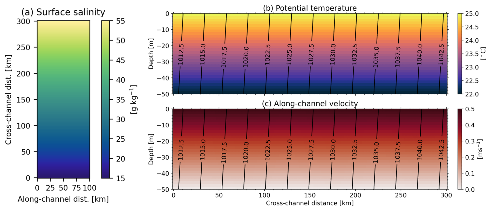
Figure 1 Initial conditions for the idealized channel domain of both models. The north-south boundaries use wall conditions, and the east-west boundaries are periodic. The 1 km ROMS mesh is used to produce the figure. (a) Surface salinity. Cross-sections of (b) potential temperature and (c) along-channel velocity with isopycnals overlaid every 2.5 kg m⁻³.

Both MPAS-O and ROMS use vertical grids with 50 equally spaced levels, giving a vertical resolution of 1 m. MPAS-O employs a z^* coordinate within an arbitrary Eulerian–Lagrangian framework (Petersen et al., 2015), while ROMS uses a terrain-following coordinate with surface and bottom stretching parameters $({\mathit{\theta }}_{\mathrm{s}},{\mathit{\theta }}_{\mathrm{b}})=\mathrm{0}$. Because the Bichan configuration uses a flat bottom, the vertical coordinates in the two models behave similarly. As a result, differences between MPAS-O and ROMS in these experiments primarily reflect their numerical schemes and subgrid-scale parameterizations rather than vertical coordinate choice. In the realistic nGoM comparison presented in Part 2, vertical coordinate differences may play a larger role. However, because bathymetric gradients on the Texas-Louisiana shelf (where the eddies are prominent) are gentle, coordinate effects should not significantly influence overall model performance. Appendix A presents a proof-of-concept demonstration of the Bichan configuration with variable bathymetry; these simulations are not part of the primary flat-bottom comparison discussed here.

Initial tracer distributions (Fig. 1a–b) of temperature, T, and salinity, S, are defined by constants, $N^{\mathrm{2}}=-g\frac{\partial \mathit{\rho }}{\partial z}{\mathit{\rho }}_{\mathrm{0}}^{-\mathrm{1}}={\mathrm{10}}^{-\mathrm{4}}{\mathrm{s}}^{-\mathrm{2}}$ and $M^{\mathrm{2}}=g\frac{\partial \mathit{\rho }}{\partial y}{\mathit{\rho }}_{\mathrm{0}}^{-\mathrm{1}}={\mathrm{10}}^{-\mathrm{6}}{\mathrm{s}}^{-\mathrm{2}}$, that define the vertical stratification and lateral density gradients,

$$\begin{array}{}\text{(1)}& {\displaystyle }T=T_{\mathrm{0}}+{\displaystyle \frac{N^{\mathrm{2}}}{g\mathit{\alpha }}}z\text{(2)}& {\displaystyle }S=S_{\mathrm{0}}+{\displaystyle \frac{M^{\mathrm{2}}}{g\mathit{\beta }}}y\end{array}$$

where T₀=25 °C, S₀=15 g kg⁻¹, α= 1.7$\times {\mathrm{10}}^{-\mathrm{4}}$ °C⁻¹ and β= 7.6$\times {\mathrm{10}}^{-\mathrm{4}}$ g⁻¹ kg are the linear thermal and haline expansion coefficients in the linearized equation of state,

$$\begin{array}{}\text{(3)}& \mathit{\rho }={\mathit{\rho }}_{\mathrm{0}}(\mathrm{1}-\mathit{\alpha }T+\mathit{\beta }S),\end{array}$$

where ρ₀=1027 kg m⁻³ is the reference density. As a result, the initial salinity varies only in cross-channel direction and temperature varies only in the vertical direction. The first deformation radius, estimated as $R_{\mathrm{d}}=Nh/f$, is approximately 5 km at the start of the simulation, similar to conditions observed on the Texas-Louisiana shelf (Hetland, 2017).

The along-channel u velocity is laterally homogeneous and is gradually relaxed from 0.5 m s⁻¹ to zero towards the bottom (Fig. 1c). The initial cross-shore velocity is set to zero. A small perturbation to the initial u velocity with a period of 100 km in both the along- and cross-channel directions and an amplitude of 0.01 m s⁻¹ is applied to supply perturbations on which instabilities can form and grow.

Simulations are forced with near-inertial wind stress in the along-channel direction:

$$\begin{array}{}\text{(4)}& {\mathit{\tau }}^x={\mathit{\tau }}_{\mathrm{0}}^x\sin \left(\mathrm{0.9}ft\right),\end{array}$$

where ${\mathit{\tau }}_{\mathrm{0}}^x=\mathrm{0.1}$ Pa is the near-inertial wind stress amplitude, which is slightly stronger than values observed in the nGoM (Schlichting et al., 2024). The purpose of the wind stress is to provide some resonant, near-inertial forcing to make the model more similar to summer conditions in the nGoM and sharpen the fronts (Schlichting et al., 2024).

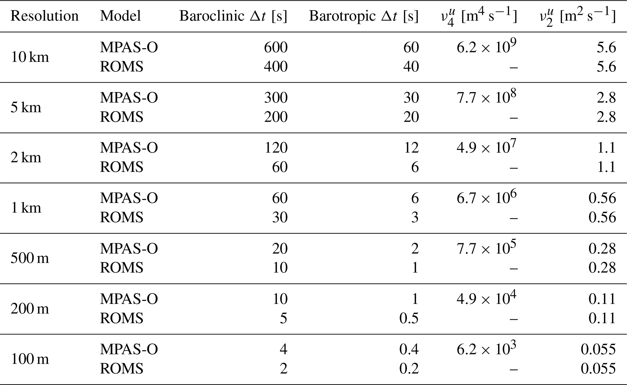
Our goal is to compare the representation of surface submesoscale dynamics between ROMS and MPAS-O across a range of resolutions ranging from mesoscale eddy-resolving to submesoscale front-resolving. To do so, we conducted a series of 50 d experiments across the following resolutions: 10, 5, 2, 1 km, 500, 200, and 100 m. Details of the model setup across resolutions are provided in the next subsections and summarized in Table 1.

Table 1 Model configuration parameters used for all MPAS-O and ROMS simulations.

2.2 MPAS-O

2.2.1 Overview

MPAS-O is a global ocean model that solves a mimetic finite-volume discretization of the primitive equations on an unstructured Arakawa C-grid (Arakawa and Lamb, 1977; Ringler et al., 2013). The horizontal mesh is generated from a planar centroidal Voronoi tessellation, producing a uniform hexagonal grid. It solves prognostic equations for momentum, layer thickness, and tracers using a vector-invariant form of the momentum equation expressed in vorticity–kinetic energy form (Arakawa and Lamb, 1977). MPAS-O vE3SM3.0.0 is configured from a branch that introduces minor changes relative to the formally described model of Golaz et al. (2026). These include the use of a free-slip wall boundary condition (instead of a no-slip condition) and the addition of the online discrete variance decay diagnostics (DVD) by Burchard and Rennau (2008) (Fig. 1).

2.2.2 Momentum advection

Momentum advection in MPAS-Ocean is computed using an energy-conserving, vector-invariant discretization based on the TRiSK framework (Ringler et al., 2010; Thuburn et al., 2009). The scheme is nominally second-order centered in space and ensures conservation of kinetic energy and potential enstrophy. However, because the advection operator is non-dissipative, explicit eddy viscosity is required to control grid-scale numerical oscillations. This is further discussed in Sect. 2.2.5. A quadratic bottom drag stress parameterization with a drag coefficient of 0.0015 is used.

2.2.3 Time integration

A split-explicit scheme is used (Ringler et al., 2013), in which the barotropic system is integrated using a second-order forward–backward method (Higdon, 2005), while the baroclinic tendencies are advanced with a second-order Adams–Bashforth scheme. Coupling between barotropic and baroclinic modes is achieved via a rectangular barotropic filter.

2.2.4 Tracer advection

A Flux-Corrected Transport (FCT) scheme following Petersen et al. (2015); Skamarock and Gassmann (2011) is used. In this scheme, a low-order monotone flux (typically upwind) is first computed, and a high-order flux – based on third- or fourth-order reconstructions – is then corrected using the low-order flux to ensure monotonicity. This approach is applied separately to both horizontal and vertical transport (Petersen et al., 2019).

2.2.5 Mixing parameterizations

Given the centered-difference approach used in MPAS-O to discretize the vector-invariant momentum advection terms, explicit horizontal momentum mixing is required to prevent spurious kinetic energy and tracer variance from accumulating at the grid scale, which can lead to an unphysical ocean state (Ilıcak et al., 2012; Megann and Storkey, 2021). MPAS-O supports Laplacian and biharmonic viscosity closures, providing second- and fourth-order dissipation, respectively (Calandrini et al., 2021). An option for the grid-scale and flow-aware Leith viscosity (Leith, 1996) is also available; however, it has not been tuned and is beyond the scope of the current study. For models that require specified background horizontal mixing for numerical robustness, like MPAS-O, this leads to a conundrum where specified background mixing may be at once too much – smoothing out important small scale features, like fronts – while at the same time never enough – as reasonable values of specified background mixing for the solution as a whole still allow numerical dispersion and associated grid scale noise at the smallest scales.

To guide the choice of viscosity coefficients and quantify the strength of explicit horizontal mixing, we use the grid Reynolds number, defined as the ratio of horizontal inertial forces to horizontal viscous forces at the grid scale. Harmonic (ν₂∇²u) and biharmonic (ν₄∇⁴u) dissipation act on larger and smaller scales, respectively. For a given simulation, the coefficients ν₂ and ν₄ are held constant and scaled according to the grid cell resolution (Δx) relative to a reference cell width (Δx_ref). Here, Δx_ref was set to 30 km, comparable to values used in previous high-resolution MPAS-O studies (Ringler et al., 2013) and roughly twice the values commonly employed in 30 km ($\mathrm{1}/\mathrm{4}\mathit{°}$) NEMO simulations (Megann and Storkey, 2021):

$$\begin{array}{}\text{(5)}& {\displaystyle }{\mathit{\nu }}_{\mathrm{2}}^u=\mathrm{3.33}\times {\mathrm{10}}^{\mathrm{1}}({\displaystyle \frac{\mathrm{\Delta }x}{\mathrm{\Delta }{x}_{\mathrm{ref}}}}{)}^{\mathrm{1}}\times {\displaystyle \frac{\mathrm{1}}{\mathrm{2}}}\text{(6)}& {\displaystyle }{\mathit{\nu }}_{\mathrm{4}}^u=\mathrm{3.33}\times {\mathrm{10}}^{\mathrm{11}}({\displaystyle \frac{\mathrm{\Delta }x}{\mathrm{\Delta }{x}_{\mathrm{ref}}}}{)}^{\mathrm{3}}\times {\displaystyle \frac{\mathrm{1}}{\mathrm{2}}}.\end{array}$$

The grid Reynolds number Re_Δ is calculated using the biharmonic viscosity coefficient, since it dominates grid-scale dissipation:

$$\begin{array}{}\text{(7)}& R{e}_{\mathrm{\Delta }}={\displaystyle \frac{\mathit{U}\left(\mathrm{\Delta }{x}^{\mathrm{3}}\right)}{\mathrm{8}{\mathit{\nu }}_{\mathrm{4}}^u}},\end{array}$$

where U is a horizontal velocity scale. Because U has multiple meanings for eddying flows, we computed probability density functions of Re_Δ using the surface grid-scale velocities (not shown) and found a mean value of 20 across all simulations, comparable to assuming U=1 m s⁻¹. While Ilıcak et al. (2012) recommends Re_Δ≤10, these values were based on tuning experiments of MPAS-O at coarser resolutions; the consequences are discussed in Sect. 3. No explicit horizontal mixing is applied to tracers.

Vertical mixing in MPAS-O is parameterized using the K-Profile Parameterization (KPP) via the Community Vertical Mixing library (CVMix; Large et al., 1994; Van Roekel et al., 2018). The ocean surface boundary layer (OSBL) is diagnosed using a critical bulk Richardson number of 0.25, with boundary layer depth and vertical mixing profiles computed using the “SimpleShapes” option and quadratic interpolation to the OSBL base. Convective mixing is triggered under unstable stratification and is scaled based on the local buoyancy frequency. Shear-driven mixing in the interior is also parameterized using KPP, with coefficients set by the critical Richardson number and velocity shear. A background viscosity of 10⁻⁴ m² s⁻¹ and diffusivity of 10⁻⁵ m² s⁻¹ are applied outside the OSBL. Additional options, such as horizontal smoothing of Richardson number profiles and the Bryan–Lewis interior mixing scheme, are enabled to provide smooth transitions between boundary layer and interior mixing.

2.3 ROMS

2.3.1 Overview

ROMS is a limited-domain structured grid ocean model with stretched terrain-following vertical coordinates that operates on an Arakawa C-Grid (Arakawa and Lamb, 1977; Shchepetkin and McWilliams, 2005), and allows nesting to better resolve regions of increased spatial resolution. ROMS v4.2 is configured using a branch derived from the ROMS-Rutgers implementation with a modification to the DVD diagnostics. This modification is described in Sect. 2.4.3.

2.3.2 Momentum advection

The simulations here use a third-order upwind scheme in the horizontal and fourth-order centered scheme in the vertical (Shchepetkin and McWilliams, 1998). In addition, a quadratic bottom stress parametrization with a drag coefficient of 0.0015 is applied, matching MPAS-O.

2.3.3 Time integration

The baroclinic mode is stepped with a third-order Adams Bashforth scheme. The barotropic mode is stepped with a third-order Leapfrog Adams Moulton scheme with forward-backward feedback. Tracers are stepped with Leapfrog scheme with a trapezoidal corrector (Shchepetkin and McWilliams, 2009).

2.3.4 Tracer advection

Multidimensional Positive Definite Advection Transport Algorithm (MPDATA) is used for horizontal and vertical tracer advection (Smolarkiewicz and Margolin, 1998). Although ROMS supports several high-order tracer advection schemes, MPDATA was selected due to its success in previous studies of submesoscale baroclinic instabilities in realistic (Kobashi and Hetland, 2020; Qu et al., 2022; Schlichting et al., 2023) and idealized (Hetland, 2017; Schlichting et al., 2024) domains.

2.3.5 Mixing parameterizations

ROMS’ third-order upwind momentum advection scheme (Shchepetkin and McWilliams, 1998, 2005) introduces implicit fourth-order biharmonic dissipation. This dissipation is grid-scale and flow-aware such that it depends on the local velocity, grid spacing, and flow direction relative to the grid. For this reason, high-resolution limited domain and estuarine ROMS configurations usually employ a small amount of explicit horizontal mixing to reduce grid-scale noise not damped by the implicit dissipation (Schlichting et al., 2023, 2024). ROMS supports options for explicit harmonic and biharmonic horizontal mixing of momentum and tracers, but they cannot be used simultaneously. The simulations here use harmonic mixing of momentum aligned with the terrain-following surfaces based on its success in previous studies of submesoscale dynamics in realistic and idealized domains (Broatch and MacCready, 2022; Kobashi and Hetland, 2020; Schlichting et al., 2024). The values of ${\mathit{\nu }}_{\mathrm{h}}^{\mathrm{2}}$ are shown in Table 1 and mimic those selected for MPAS-O simulations. No explicit horizontal mixing is applied to the tracers.

For vertical mixing, ROMS' native KPP scheme is used, which provides the closest available comparison to the standardized and portable KPP formulation included in the MPAS-Ocean configuration that uses the CVMix library (Large et al., 1994; Van Roekel et al., 2018). Although both approaches follow the general structure of Large et al. (1994), several notable algorithmic and numerical differences exist between them. As highlighted in previous studies (Li et al., 2019; Robertson and Dong, 2019), the ROMS implementation is more tightly hard-coded and less configurable than CVMix, and these differences can lead to divergent solutions even in idealized one-dimensional tests.

A full description of all distinctions between the KPP implementations is beyond the scope of this paper; here we briefly note that ROMS differs in its calculation of the ocean surface boundary-layer depth, its boundary-layer shape functions for turbulent diffusivities and nonlocal fluxes, and its treatment of convective adjustment in unstable columns. Shear-driven mixing in the interior is based on bulk Richardson-number-dependent diffusivities and viscosities, with options for horizontal and vertical averaging to improve numerical stability. A Shapiro filter is applied to the vertical mixing coefficients to suppress spurious oscillations and smooth the profiles, which are then interpolated to the vertical velocity cell faces using cubic splines.

2.4 Analysis methods

We apply multiple techniques to compare physical dynamics for all model simulations which include surface and volume integrated energetics, measures of flow invariants, and diagnostics of physical and numerical mixing. Details for each of these are provided in the subsections below.

2.4.1 Energetics

We compute surface kinetic energy (KE) levels as well as volume-integrated eddy kinetic energy (EKE) over the 50 d simulation period between 50 and 250 km in the y-direction to avoid wall effects. EKE is normalized by mean kinetic energy at the initial timestep, computed as

$$\begin{array}{}\text{(8)}& \mathrm{EKE}={\displaystyle \frac{\iiint \frac{\mathrm{1}}{\mathrm{2}}\left[(\mathit{u}-\stackrel{\mathrm{‾}}{\mathit{u}}{)}^{\mathrm{2}}+(\mathit{v}-\stackrel{\mathrm{‾}}{\mathit{v}}{)}^{\mathrm{2}}\right]\mathrm{d}V}{\iiint \frac{\mathrm{1}}{\mathrm{2}}\left[{\stackrel{\mathrm{‾}}{\mathit{u}}}_{t=\mathrm{0}}^{\mathrm{2}}+{\stackrel{\mathrm{‾}}{\mathit{v}}}_{t=\mathrm{0}}^{\mathrm{2}}\right]\mathrm{d}V}}.\end{array}$$

where $\stackrel{\mathrm{‾}}{\mathit{u}}$ and $\stackrel{\mathrm{‾}}{\mathit{v}}$ represented the volume weighted zonal means of each velocity component. Time series of both KE and EKE are smoothed using a low-pass PL33 filter (Flagg et al., 1976), though the raw values are also retained and utilized to compute the maximum 10 d average period over which flow invariants are analyzed.

2.4.2 Flow invariants

Analyses of the experimental results are computed over the surface layer for total kinetic energy, and histograms of relative vorticity, ζ, divergence, δ, and total strain, σ, defined as

$$\begin{array}{}\text{(9)}& {\displaystyle }\mathit{\zeta }={\displaystyle \frac{\partial v}{\partial x}}-{\displaystyle \frac{\partial u}{\partial y}}\text{(10)}& {\displaystyle }\mathit{\delta }={\displaystyle \frac{\partial u}{\partial x}}+{\displaystyle \frac{\partial v}{\partial y}}\text{(11)}& {\displaystyle }\mathit{\sigma }=\sqrt{{\mathit{\sigma }}_{\mathrm{n}}^{\mathrm{2}}+{\mathit{\sigma }}_{\mathrm{s}}^{\mathrm{2}}},\end{array}$$

where σ_n and σ_s correspond to the components of normal strain ${\mathit{\sigma }}_{\mathrm{n}}=\frac{\partial u}{\partial x}-\frac{\partial v}{\partial y}$ and shear strain ${\mathit{\sigma }}_{\mathrm{s}}=\frac{\partial v}{\partial x}+\frac{\partial u}{\partial y}$, respectively. These flow invariants are commonly used and allow us to interpret our simulations in the context of previous studies (e.g., Shcherbina et al., 2013b).

Comprehensive analyses of frontogenesis can also help identify the capability of models to capture nonlinear processes at multiple spatial resolutions, providing a rigorous test of effective resolution between models where vertical mixing, or the irreversible loss of vertical stratification, is most strongly affected. Therefore, analyses of frontogenesis were conducted following the methodology of Hetland et al. (2025) which computes histograms within the coordinates of the front. The cross- and along-frontal velocity components within this coordinate system are denoted by $\stackrel{\mathrm{̃}}{\mathit{u}}$ and $\stackrel{\mathrm{̃}}{\mathit{v}}$, respectively, which correspond to the frontal coordinate directions ($\stackrel{\mathrm{̃}}{x}$ and $\stackrel{\mathrm{̃}}{y}$) that are rotated by the angle α from regular Cartesian coordinates (x and y, see Fig. 1 in Hetland et al., 2025),

$$\begin{array}{}\text{(12)}& {\displaystyle }\stackrel{\mathrm{̃}}{\mathit{u}}=\mathit{u}\cos \mathit{\alpha }+\mathit{v}\sin \mathit{\alpha }\text{(13)}& {\displaystyle }\stackrel{\mathrm{̃}}{\mathit{v}}=-\mathit{u}\sin \mathit{\alpha }+\mathit{v}\cos \mathit{\alpha }.\end{array}$$

The cross-frontal gradient of $\stackrel{\mathrm{̃}}{\mathit{u}}$ can then be defined in frontal coordinates as well,

$$\begin{array}{}\text{(14)}& \begin{array}{rl}{\displaystyle \frac{\partial \stackrel{\mathrm{̃}}{u}}{\partial \stackrel{\mathrm{̃}}{x}}}& ={\displaystyle \frac{\partial u}{\partial \stackrel{\mathrm{̃}}{x}}}\cos \mathit{\alpha }+{\displaystyle \frac{\partial v}{\partial \stackrel{\mathrm{̃}}{x}}}\sin \mathit{\alpha }\\ & =\left({\displaystyle \frac{\partial u}{\partial x}}{\displaystyle \frac{\partial x}{\partial \stackrel{\mathrm{̃}}{x}}}+{\displaystyle \frac{\partial u}{\partial y}}{\displaystyle \frac{\partial y}{\partial \stackrel{\mathrm{̃}}{x}}}\right)\cos \mathit{\alpha }+\left({\displaystyle \frac{\partial v}{\partial x}}{\displaystyle \frac{\partial x}{\partial \stackrel{\mathrm{̃}}{x}}}+{\displaystyle \frac{\partial v}{\partial y}}{\displaystyle \frac{\partial y}{\partial \stackrel{\mathrm{̃}}{x}}}\right)\sin \mathit{\alpha }\\ & =u_x{\cos }^{\mathrm{2}}\mathit{\alpha }+u_y\sin \mathit{\alpha }\cos \mathit{\alpha }+v_x\sin \mathit{\alpha }\cos \mathit{\alpha }\\ & +v_y{\sin }^{\mathrm{2}}\mathit{\alpha }.\end{array}\end{array}$$

This is equivalent to the negative of the frontogenesis function, with $-\stackrel{\mathrm{̃}}{\mathit{u}}$ defining the rate of frontal sharpening. Following similar steps, the along-front gradient rotated to local frontal coordinates can be expressed as

$$\begin{array}{}\text{(15)}& \begin{array}{rl}{\displaystyle \frac{\partial \stackrel{\mathrm{̃}}{v}}{\partial \stackrel{\mathrm{̃}}{y}}}& =u_x{\sin }^{\mathrm{2}}\mathit{\alpha }-u_y\sin \mathit{\alpha }\cos \mathit{\alpha }-v_x\sin \mathit{\alpha }\cos \mathit{\alpha }\\ & +v_y{\cos }^{\mathrm{2}}\mathit{\alpha }.\end{array}\end{array}$$

Along-channel means and standard deviations of velocities and tracers are also computed over a 10 d window centered around average peak surface kinetic energy levels. Like KE and EKE, probability density functions are computed over the surface level of the model domain between 50 and 250 km in the y-direction, and are analyzed over the same 10 d period during which the average generation of frontal processes across multiple resolutions is maximized.

2.4.3 Mixing diagnostics

We focus on numerical and physical salinity mixing because the density variations are dominated by salinity variations (Fig. 1). Online mixing diagnostics have been previously implemented and validated in ROMS (Kalra et al., 2019). They have been added into MPAS-O for this study and future work. Physical mixing for these simulations is given by

$$\begin{array}{}\text{(16)}& {\mathcal{M}}_{\mathrm{phy}}=\mathrm{2}{\mathit{\kappa }}_{\mathrm{v}}{\left({\displaystyle \frac{\partial s}{\partial z}}\right)}^{\mathrm{2}}\end{array}$$

where κ_v is the vertical tracer diffusivity. The validation of ℳ_phy is not shown for MPAS-O because it simply requires ensuring online and offline calculations (snapshots) agree to machine precision. We note that previous ROMS versions calculated ℳ_phy using the resolved diffusivity κ_v−κ₀, where κ₀ is the background vertical diffusivity. Instead, we use the total diffusivity κ_v so that all prescribed processes that destroy tracer variance are represented.

Numerical salinity mixing is quantified using the DVD algorithm by Burchard and Rennau (2008):

$$\begin{array}{}\text{(17)}& {\mathcal{M}}_{\mathrm{num}}={\displaystyle \frac{A\left\{(s{)}^{\mathrm{2}}\right\}-{\left(A\left\{s\right\}\right)}^{\mathrm{2}}}{\mathrm{\Delta }t}}.\end{array}$$

where A{.} is the advection operator and Δt is the baroclinic timestep. The advection operator is equal to the updated concentration of the tracer c when passed solely through the advection scheme. In both models, numerical mixing diagnostics are currently supported only for active tracers. In practice, this requires introducing two additional tracers per active tracer, initialized with c and c², for which all tracer tendencies other than advection (e.g., implicit vertical mixing) are disabled. For this study, we implemented and verified it for MPAS-O by comparing online diagnostics of ℳ_num with a tracer variance budget residual approach for the advection of a top-hat tracer distribution (see Appendix B).

Local estimates of ℳ_num can be contaminated by implicit diffusion and by variance changes associated with fluxes across cell interfaces, which makes them inherently noisy; however, when integrated over the full domain, these contributions cancel exactly, yielding a global variance decay calculation that closes to machine precision (Banerjee et al., 2024; Klingbeil et al., 2014). More computationally efficient DVD algorithms exist (referenced above) that are thought to be more accurate at the grid scale, but they have not been implemented in ROMS or MPAS-O yet because of their complexity. Despite these differences, no method produces fully consistent local results; however, all approaches are believed to provide similar bulk (volume-integrated) ℳ_num. Each approach recommends applying spatial and/or temporal averaging to local ℳ_num fields to reduce grid-scale noise. However, because the channel configuration contains rapidly evolving, multiscale eddies, it is unclear how to define a grid- and flow-aware average that selectively removes grid-scale noise without smearing out the “true” numerical mixing. To partially alleviate the grid-scale noise, we use averages saved every two hours (the same frequency as snapshots) for mixing related calculations.

3 Results

3.1 Energetics and flow invariants

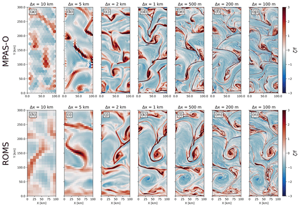
The representation of submesoscale dynamics varies strongly with horizontal resolution, highlighted by surface relative vorticities during a period of high kinetic energy for both models (Day 12, Fig. 2) where submesoscale fronts (𝒪 1–10 km) and eddies (𝒪 50 km, roughly 10 times the deformation radius) emerge across all resolutions. Inter-model comparisons at each resolution shows qualitatively similar results in the representation of eddy and frontal dynamics for both MPAS-O and ROMS. At 5–10 km resolutions (Fig. 2a–b, h–i), which we consider eddy-permitting, the representation of submesoscale frontal processes is limited by both ocean models. At 1–2 km resolutions (Fig. 2c–d, j–k), which we consider to be eddy-resolving, relative vorticity magnitude increases and frontal instabilities emerge in both models – dark red areas that appear “braided”. At sub-kilometer resolutions (Fig. 2e–g, l–n), resolution is sufficient to resolve cross-frontal processes and frontal instabilities become more complex in both models. The imprint of gravity waves propagating away from frontal convergence zones in regions with anticyclonic vorticity becomes apparent at 100–200 m resolutions for both models (Fig. 2f–g, m–n).

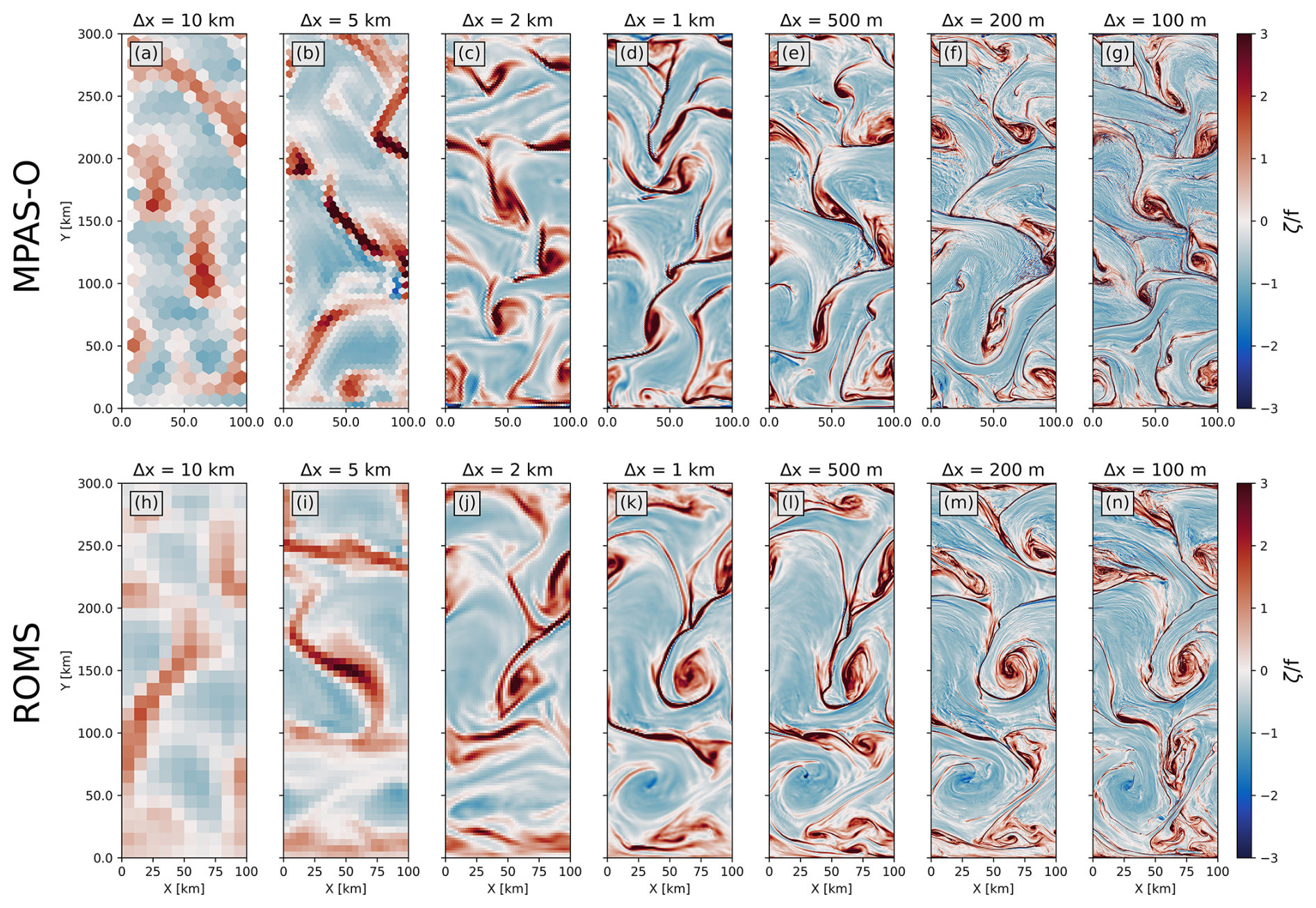
Figure 2 Snapshots of surface normalized relative vorticity (ζf⁻¹) plots for MPAS-O (a–g) and ROMS (h–n) on Day 12.

The persistence in the location of fronts is evident in the ROMS simulations as spatial resolution is refined from 1 km to 100 m (Fig. 2k–n). Generally, better defined frontal structures result in greater variability at finer spatial resolutions within the front itself. Similarities in the locations of fronts in MPAS-O at the same time are much less apparent compared to the ROMS simulations, although there is greater spatial coherence in MPAS-O among some of the fine-scale (100–200 m) simulations at earlier time periods (see animations of both simulations in the data archive). This relative lack of spatial coherence in MPAS-O is likely due to unavoidable highly nonlinear grid-scale processes (further elaborated on in the discussion) that help define early differences in initial conditions that then rapidly evolve. Like the fine-scale ROMS simulations (Fig. 2m–n), comparable MPAS-O results show greater variability within frontal regions (Fig. 2f–g).

Grid-scale noise emerges in MPAS-O at sub-kilometer resolutions (Fig. 2e–g), where it organizes into wave-like structures similar to Gibbs phenomenon. This noise is much weaker in the 500 m simulation and increases with increasing resolution. These results suggest that the biharmonic viscosity, which dissipates energy at the smallest resolved scales and is controlled by the grid Reynolds number, requires retuning at sub-kilometer resolutions for the new second-order Adams-Bashforth time-stepping scheme. A grid Reynolds number of 20 was tuned for the original split-explicit time stepping (Ringler et al., 2013) and is commonly used in various MPAS-O configurations. A systematic retuning is beyond the scope of this study due to the substantial computational and storage costs of the 100–200 m simulations; for example, the 100 m simulation requires nearly six days of wall-clock time on 4096 cores and produces 11 TB of output. The impacts of this grid-scale noise are discussed throughout the paper.

The emergence of energetic submesoscale frontal processes occurs more rapidly in ROMS than MPAS-O, evidenced by time series of surface domain-averaged kinetic energy (KE) and depth-integrated eddy kinetic energy (EKE) across all resolutions (Fig. 3). Low levels of KE and EKE are simulated during the first 4–5 d for both MPAS-O and ROMS simulations. At approximately Day 5, however, the mean surface KE in the ROMS model domain rapidly increases, peaking around Day 10 at 0.65 m² s⁻² for all sub-kilometer resolution scenarios (Fig. 3b). This average peak in MPAS-O mean surface KE occurs 4 d later than ROMS, at similar levels (Fig. 3a). MPAS-O simulations also decrease surface KE more rapidly but reach approximately the same endpoint as ROMS simulations over the remainder of the 50 d period, although both 10 km model scenarios decay most rapidly and reach a lower stable endpoint (Fig. 3a–b). This pattern, however, does not hold for EKE time series, which peak at higher levels for coarser resolutions in MPAS-O than ROMS, with generally less stability for most resolutions (Fig. 3c–d). Generally, there is greater variability in the absolute value of surface KE across model resolutions for ROMS than MPAS-O over the first half of the simulation period. For EKE, the trend towards a lower stable configuration is more variable for a greater number of spatial resolutions in ROMS, but MPAS-O has a noticeable uptick in the highest resolution (100 m) simulation, likely a spurious mode that emerges as grid-scale tracer variance becomes more important. A key detail not reflected in Fig. 3 is that there is there is much less structure within and surrounding fronts in MPAS-O compared to ROMS beyond the halfway point in the simulations (∼ Day 25, see data archive animations). We return to this point again in Sect. 3.2.

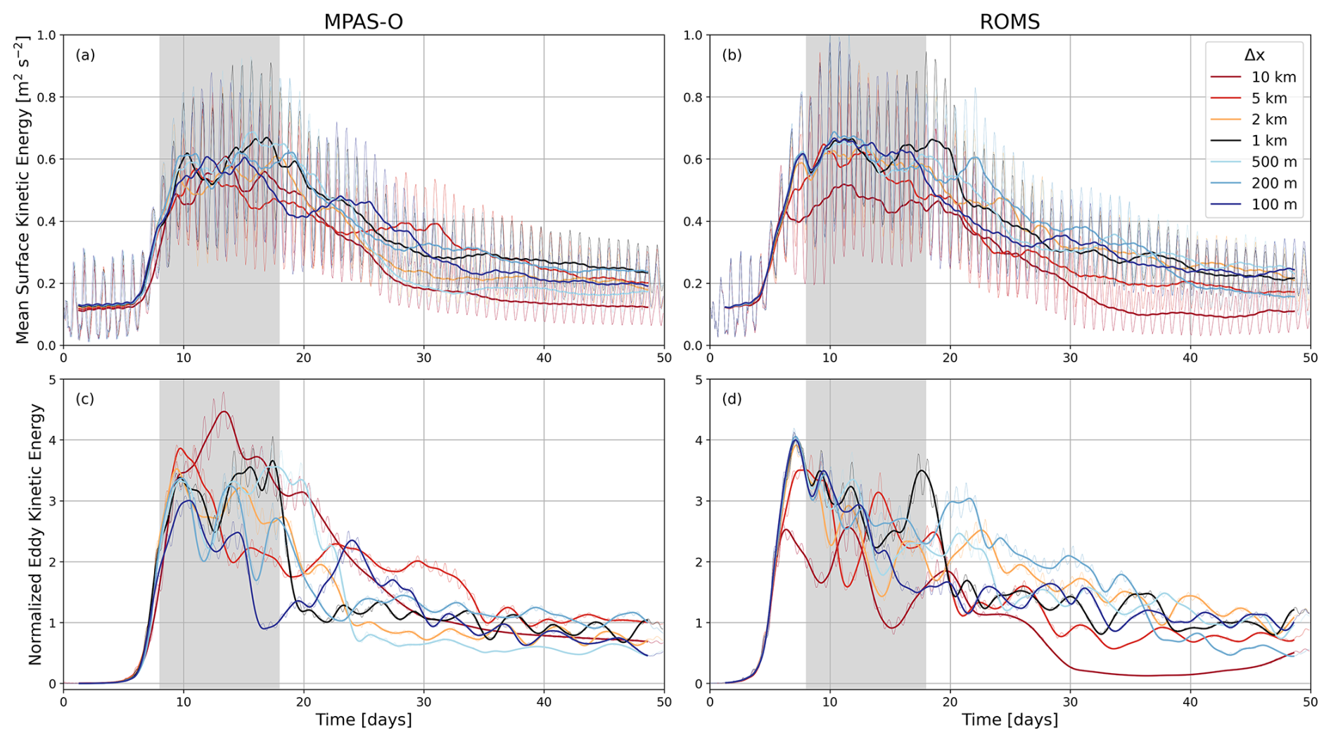
Figure 3 Time series of mean surface KE for MPAS-O (a) and ROMS (b) simulations over a range of spatial resolutions. Time series of normalized eddy kinetic energy (EKE) are shown for MPAS-O (c) and ROMS (d). Thicker lines show the KE time series smoothed with a PL33 filter while the lighter lines show the unfiltered data. Gray shaded regions in all panels correspond to the average maximum 10 d period of KE (Day 8–18) that is analyzed in subsequent histogram plots.

The kinetic energy spectra (Fig. 4) computed over the entirety of the simulation also reinforces that ROMS has slightly greater levels of regular high frequency variability compared to MPAS-O. Both ocean models show a clearly defined subinertial peak in their spectra, closely matching the imposed periodic wind forcings. At lower frequencies, the two models are highly similar at 1 km resolution; generally differences in the KE spectra distributions between the two ocean models are smaller than the differences in distribution for an ocean model across multiple spatial resolutions. While the amplitude of high-frequency (near daily) variability in surface KE is greater for ROMS than MPAS-O in the first month of the simulation, this difference is diminished by Day 40 (3a–b), as both models converge to surface KE levels that are only slightly greater than initial conditions as the strong salinity gradients are progressively eroded. The average 10 d periods of maximum surface KE for both models (Day 8–18) are banded in gray (Fig. 3a–b) and these subsets of the simulations are used for calculations in the remaining analyses.

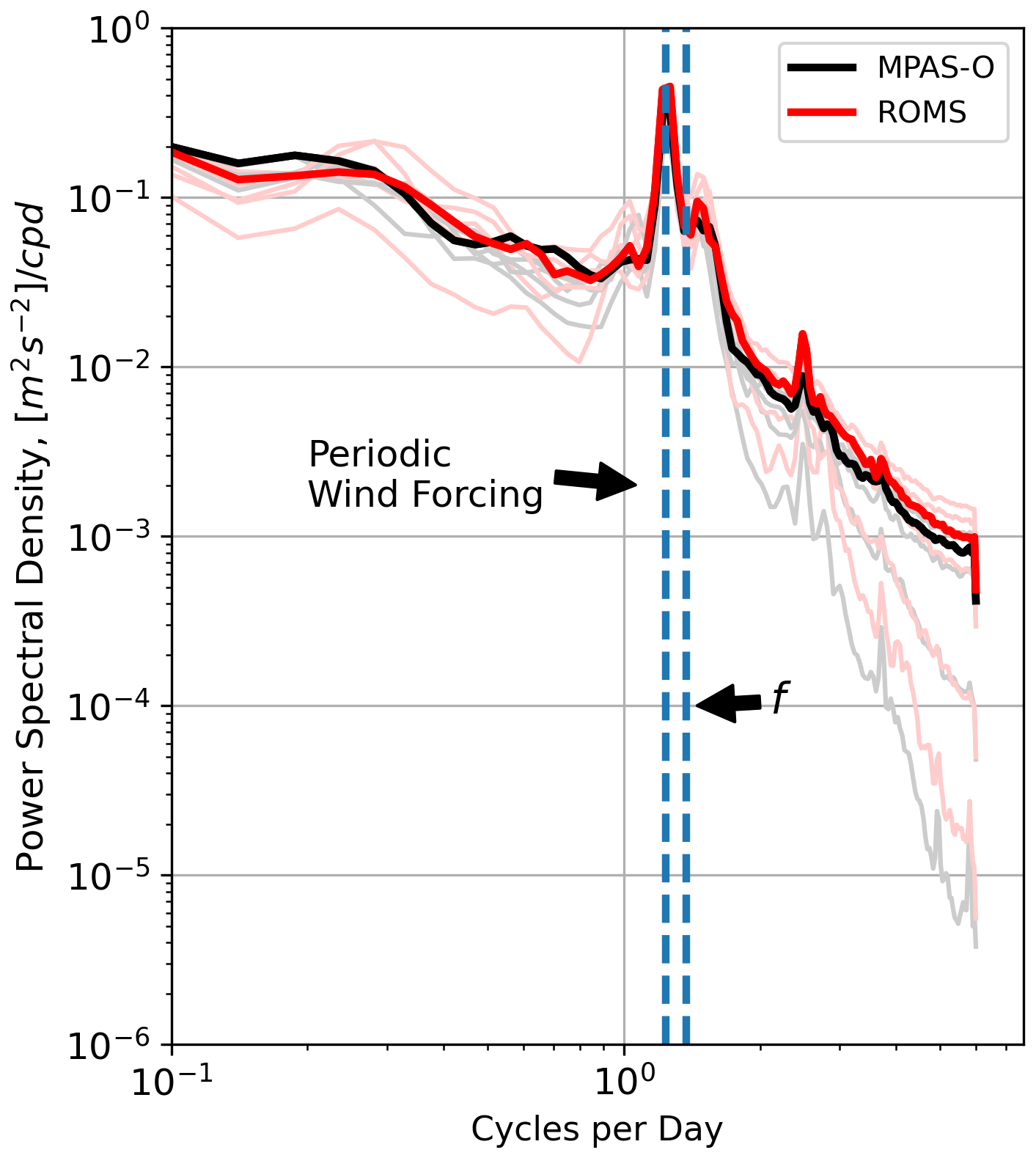
Figure 4 Power density spectra of the time series for MPAS-O (black lines) and ROMS (red lines) where the thicker lines for both models show the 1 km spatial resolution spectra and thinner lines represent all other spatial resolutions. Dashed lines correspond to the frequencies of the periodic wind forcing and Coriolis term.

Surface relative vorticity and divergence dynamics demonstrate similar shifts in their distributions due to increasing resolution for both MPAS-O and ROMS (Fig. 5) over the 10 d period when surface mean KE is maximized (Fig. 3). At coarse spatial resolutions, the PDF of relative vorticity (Fig. 5a–b) is slightly positively skewed with a shorter positive tail, indicating lower levels of frontogenesis. In both models, this skew also becomes more positive at higher spatial resolutions, and is slightly more peaked in negative vorticity for MPAS-O than ROMS at equivalent resolutions with the exception of the 100 m scenario. This elevated peak in MPAS-O negative $\mathit{\zeta }/f$ is indicative of a sharper division between eddies and frontal regions in ROMS simulations at higher spatial resolutions compared to smoother gradients found in MPAS-O. Both models also show a distinctive asymmetric shift leftwards at resolutions finer than 5 km, with the highest peak in negative vorticity occurring for both models' 500 m simulations.

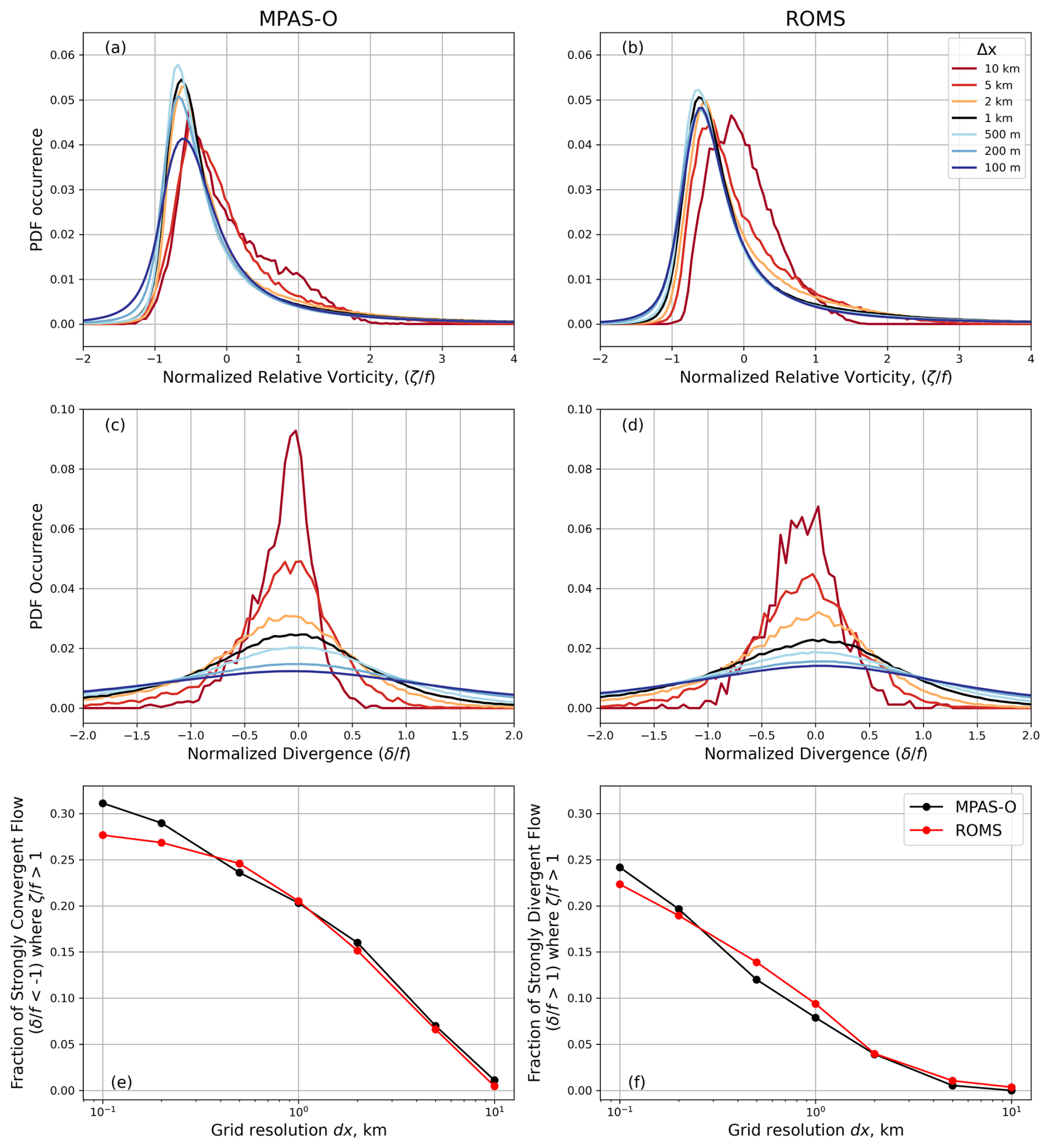
Figure 5 PDFs of surface relative vorticity (a, b) and surface divergence within fronts where ζ>1 (c, d) for MPAS-O (a, c) and ROMS (b, d) simulations over a range of spatial resolutions. Negative relative vorticity values correspond to a greater amount of anticyclonic flows characterized by eddy activity, while positive vorticity values are associated with frontal processes. Fraction of strongly convergent (e) and strongly divergent (f) flow along fronts at all spatial resolutions for MPAS-O (black) and ROMS (red).

The distributions of normalized divergence within fronts (where $\mathit{\zeta }{f}^{-\mathrm{1}}>\mathrm{1}$, Fig. 5c–f) again emphasize that inter-model differences between MPAS-O and ROMS are smaller than intra-model spatial resolution differences. In both models, coarser spatial resolutions produced a lesser amount of fronts (locations where $\mathit{\zeta }{f}^{-\mathrm{1}}>\mathrm{1}$), resulting in lower levels of divergence (positive x axis) and convergence (negative x axis) than more highly spatially resolved simulations. There is also a marked change in the distributions of divergence as spatial resolution decreases below 1 km, where the distribution is severely flattened and extends outwards beyond $-\mathrm{1}<\mathit{\delta }{f}^{-\mathrm{1}}<\mathrm{1}$. Both models show that the vast majority (> 96 %) of convergent flows fall within ±1 at spatial resolutions of 10 and 5 km (Fig. 5e).

The relative fractions of convergent flow along fronts ($\mathit{\zeta }{f}^{-\mathrm{1}}>\mathrm{1}$) in ROMS and MPAS-O are approximately equal across all simulations ≥ 1 km (Fig. 5e). At highly resolved (100–200 m) resolutions, MPAS-O has slightly greater amounts of strongly convergent flow, suggesting a growing influence of grid-scale noise. The fraction of strongly divergent flows are also similar between models across all spatial resolutions (Fig. 5f). At spatial resolutions of 100 m, the percentage of strongly divergent and convergent flows along fronts ($\left|\mathit{\delta }{f}^{-\mathrm{1}}\right|>\mathrm{1}$ where $\mathit{\zeta }{f}^{-\mathrm{1}}>\mathrm{1}$) in MPAS-O and ROMS (the sum of the left-most values in panels e and f) are equal to 55 % and 50 %, respectively.

Joint PDFs of vorticity versus strain rate (Fig. 6) and divergence (Fig. 7), following that described by Shcherbina et al. (2013b), demonstrate similar behavior under periodic wind stress conditions for MPAS-O and ROMS. In both models, increasing spatial resolution increases the strength of the relationship between increasing positive vorticities and strain rates, centered around the dashed gray line at 45° highlighting regions of pure shear that are characterized by strong cyclonic vorticity (Fig. 6). As spatial resolution increases, the relationship along this line of pure shear becomes less distinctive in both MPAS-O and ROMS. However, a clear divide between relative vorticity values at −1 (where ζ is equal to −f at the zero potential vorticity boundary) remains apparent across resolutions, although this is more visible within ROMS than MPAS-O. This is most clearly exemplified by a clear increase in shear associated with low negative relative vorticities at high spatial resolutions in MPAS-O (Fig. 6d) that is also present but substantially diminished in ROMS (Fig. 6h).

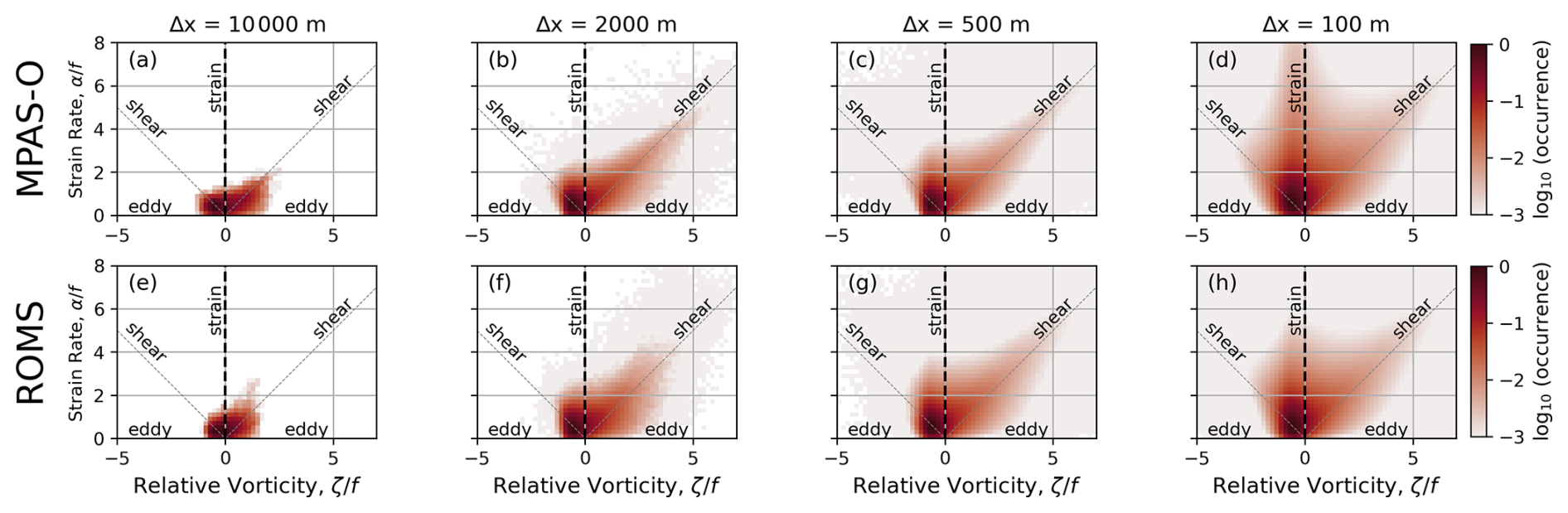
Figure 6 Joint PDFs of surface strain vs surface relative vorticity for MPAS-O (a–d) and ROMS (e–h) simulations over a range of spatial resolutions. Colorbar denotes, in log scale, the frequency of occurrence of these relationships. Diagonal gray lines emanating at 45° to the left and right of the origin denote regions of shear while the vertical line identified at x=0 corresponds to pure strain. Regions below these diagonal lines correspond to eddies in the simulations.

Relationships between normalized divergence and relative vorticity for MPAS-O and ROMS are also similar, but again highlight differences in the distributions of divergence between the two models (Fig. 7). Reflecting the differences in the shape of the PDFs (Fig. 5c–d), the distribution of divergence vs. vorticity is more narrowly focused about the x axis for MPAS-O than ROMS, which has a greater negative skew in divergence. However a clear barrier point at ζ values that are equal to −f remains evident in both models at resolutions > 100 m.

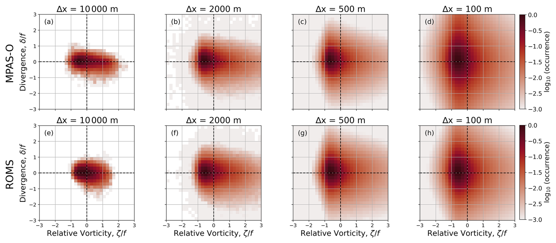
Figure 7 Joint PDFs of surface divergence vs. surface relative vorticity for MPAS-O (a–d) and ROMS (e–h) simulations over a range of spatial resolutions. Colorbar denotes, in log scale, the frequency of occurrence of these relationships.

Joint PDFs of along- and cross-frontal divergence within frontal coordinates at the surface were also computed in regions where $\mathit{\zeta }{f}^{-\mathrm{1}}>\mathrm{1}$, following the approach introduced by Hetland et al. (2025) (Fig. 8). The distributions in both MPAS-O and ROMS show a clear rotation towards a more vertically aligned distribution (greater frontal compression and decreased shear) for both ocean models as spatial resolution increases. Ellipses fit to the model variation using principal component analysis reinforce that the rotation is increasingly aligned along the axis of cross-frontal divergence as the component parallel to the major axis becomes more closely aligned with the y axis (Table 2). With smaller spatial scales, flows in both MPAS-O and ROMS become more convergent, as the primary axis of variability lies in the along-front direction of elevated vorticity regions. Differences in levels of divergence between MPAS-O and ROMS are also shown in Table 2, where the ratio of major to minor components of principal component analysis (PCA) variability show a somewhat consistent increase from coarser to finer scale ROMS simulations but mixed trends for MPAS-O simulations. This reinforces what is evident in Fig. 8, that the distribution of cross- versus along-frontal divergence values are more diffuse in MPAS-O than ROMS at all resolutions ≥ 500 m. Despite some differences in the angle of rotation of the primary axis of variability, the average of the distributions ($\partial \stackrel{\mathrm{̃}}{u}/\partial \stackrel{\mathrm{̃}}{x}$) is remarkably similar (within ±0.06) for cross-frontal divergence values between MPAS-O and ROMS across all resolutions.

Table 2 Mean properties of the surface frontal velocity gradient distributions are given for different idealized model resolutions. The rotation of the principle component major axis, ϕ_PCA, is given in degrees clockwise from the y axis; $\mathrm{major}/\mathrm{minor}$ is the ratio of the major to minor principal component axes; and $\langle \frac{\partial \stackrel{\mathrm{̃}}{u}}{\partial \stackrel{\mathrm{̃}}{x}}\rangle$ is the mean cross-frontal divergence, where negative values indicate frontogenesis.

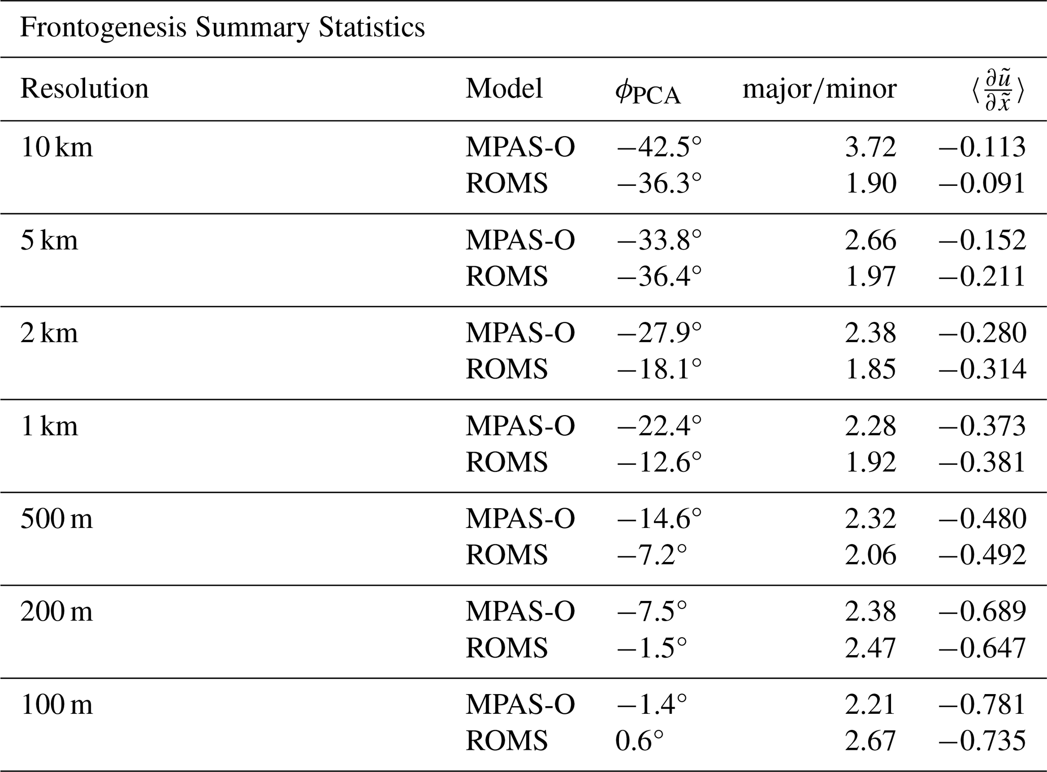
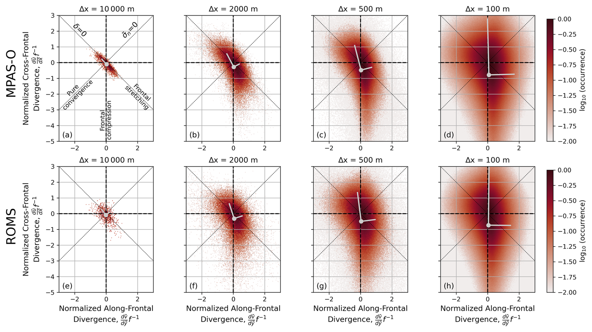
Figure 8 PDFs of normalized cross-frontal ($\frac{\partial \stackrel{\mathrm{̃}}{u}}{\partial \stackrel{\mathrm{̃}}{x}}{f}^{-\mathrm{1}}$) vs. along-frontal ($\frac{\partial \stackrel{\mathrm{̃}}{v}}{\partial \stackrel{\mathrm{̃}}{y}}{f}^{-\mathrm{1}}$) surface velocity gradients for MPAS-O (a–d) and ROMS (e–h) simulations over a range of spatial resolutions, for all points associated with frontal regions ($\mathit{\zeta }{f}^{-\mathrm{1}}>\mathrm{1}$). Colorbar denotes, in log scale, the frequency of occurrence of these relationships. Gray lines emanating from the average of these distributions (gray dots) show the principal components of variability of the distribution. The negatively sloping dashed line corresponds to zero divergence (δ=0), while the positively sloping dashed line corresponds to zero effective strain (${\stackrel{\mathrm{̃}}{\mathit{\sigma }}}_n=\mathrm{0}$).

3.2 Salinity mixing

Plan-view plots of surface numerical mixing for both models across all resolutions are shown in Fig. 9, at the same time as Fig. 2. Numerical mixing is generally largest at fronts for all resolutions due to elevated salinity gradients, consistent with previous studies (Ralston et al., 2017; Schlichting et al., 2024). At 1–10 km resolutions (Fig. 9a–d, h–k), numerical mixing is noisy at the grid scale, with the spatially-averaged mixing generally decreasing as resolution increases, particularly within eddies. At sub-kilometer resolutions in MPAS-O (Fig. 9e–g), regions with grid-scale noise in the vorticity field coincide with regions of higher numerical mixing. This is most prevalent in the 200 m simulation (Fig. 9f). Significant patches of negative numerical mixing are visible in both models, with MPAS-O showing slightly more organized patches. The negative patches indicate tracer variance production, rather than destruction, and may reflect either anti-diffusive or dispersive numerical errors associated with the advection schemes. However, we cannot precisely determine the quantity of numerical mixing occurring at the grid scale that directly results from the tracer advection scheme or noise generated by the DVD algorithm.

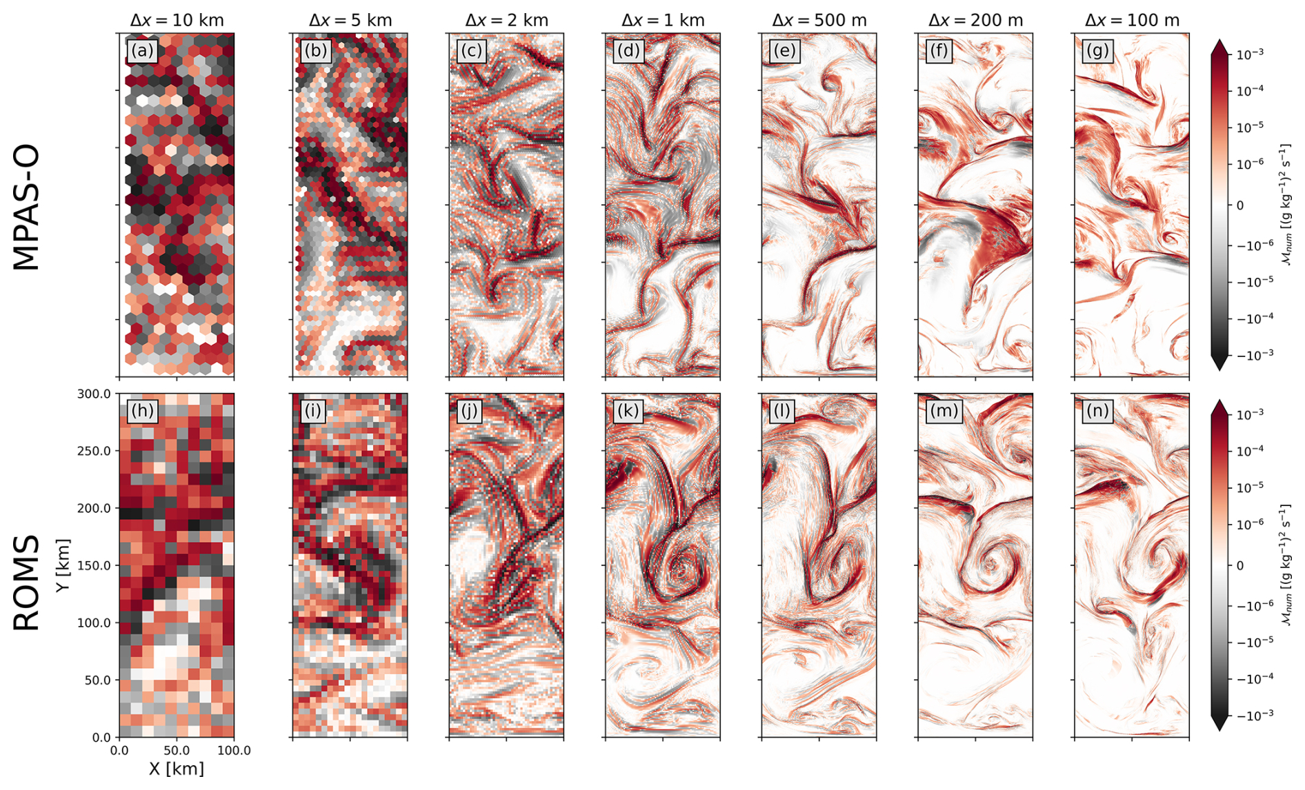
Figure 9 Surface numerical salinity mixing for MPAS-O (a–g) and ROMS (h–n) at the same time as Fig. 2.

To further quantify these differences, we examine time series of volume-averaged physical (Fig. 10a–b) and numerical (Fig. 10c–d) mixing for both models across all resolutions. The volume-averaging operator is defined as $V^{-\mathrm{1}}\iiint \mathit{\{}.\mathit{\}}\mathrm{d}V$, where V is the domain volume. The volume-averaged physical mixing is correlated with the time series of mean surface kinetic energy (Fig. 3), growing later in MPAS-O (Fig. 10a) than in ROMS (Fig. 10b). Since the models were initialized with vertically uniform salinity, physical mixing is strongly influenced by restratification due to mixed-layer instabilities (Fox-Kemper et al., 2011), which generates vertical salinity variance that can be destroyed by mixing. In MPAS-O, the volume-averaged physical mixing reaches a steady, periodic state that exceeds ROMS by the end of the simulation. Physical mixing generally increases with resolution, particularly when kinetic energy is near its maximum.

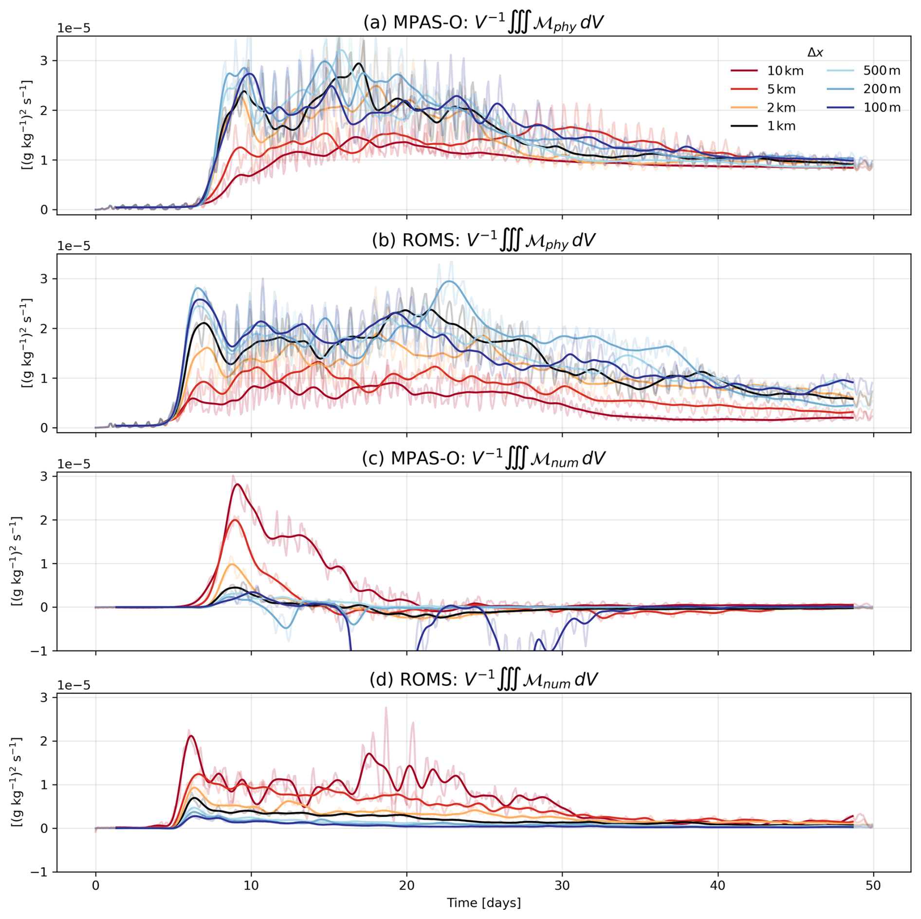
Figure 10 Time series of volume-averaged physical (a–b) and numerical (c–d) mixing for both models across all resolutions. Thicker lines are smoothed with a PL33 filter; thinner, fainter lines are the raw outputs.

Volume-averaged numerical mixing (Fig. 10c–d) partially follows the distribution of kinetic energy, peaking during eddy formation but decreasing much faster than physical mixing. This is likely because strongly convergent ageostrophic motions during frontogenesis sharpen horizontal salinity gradients. As the simulation evolves through the later phases of the frontal life cycle (instability, arrest, and decay), the destruction of salinity gradients reduces numerical mixing. For both models, volume-averaged numerical mixing generally decreases with increasing resolution, with notable exceptions. MPAS-O exhibits higher peak numerical mixing in the 2, 5, and 10 km cases than ROMS, and oscillates between positive and negative values at all resolutions. The 100–200 m simulations, especially the 100 m run, show much more tracer variance production, likely due to excessive grid-scale noise. Peak instances of negative numerical mixing for the 100 m simulation occur between Days 15–20 and Days 25–30. The behavior may be phenomenologically similar to fossil turbulence (Gibson, 1999) in that small-scale variance persists after the energetic phase, but in this case arises from numerical rather than physical processes. In ROMS, volume-averaged numerical mixing remains positive at all resolutions and consistently decreases with increasing resolution.

To summarize differences between models and across resolutions, we compute bulk mixing quantities (Fig. 11), defined as the time-summed volume-averaged mixing. We normalize horizontal resolution by the initial deformation radius (5 km) to produce a dimensionless metric which may be useful for future studies. For MPAS-O, the absolute value of numerical mixing is taken at each time step to prevent negative values from artificially reducing bulk mixing. This is preferable to taking the absolute value of numerical mixing at the grid scale because the noise from the DVD algorithm would contaminate the bulk mixing estimates. The ratio of bulk numerical to physical mixing decreases with increasing resolution (Fig. 11a), except for the 100 m MPAS-O case. In MPAS-O, this ratio decreases from 42 % at 10 km to 2.8 % at 200 m, but rises to 40 % at 100 m. In ROMS, the ratio decreases from 131 % at 10 km to 4 % at 100 m. Bulk numerical (Fig. 11b) and physical mixing (Fig. 11c) trends reflect these ratios.

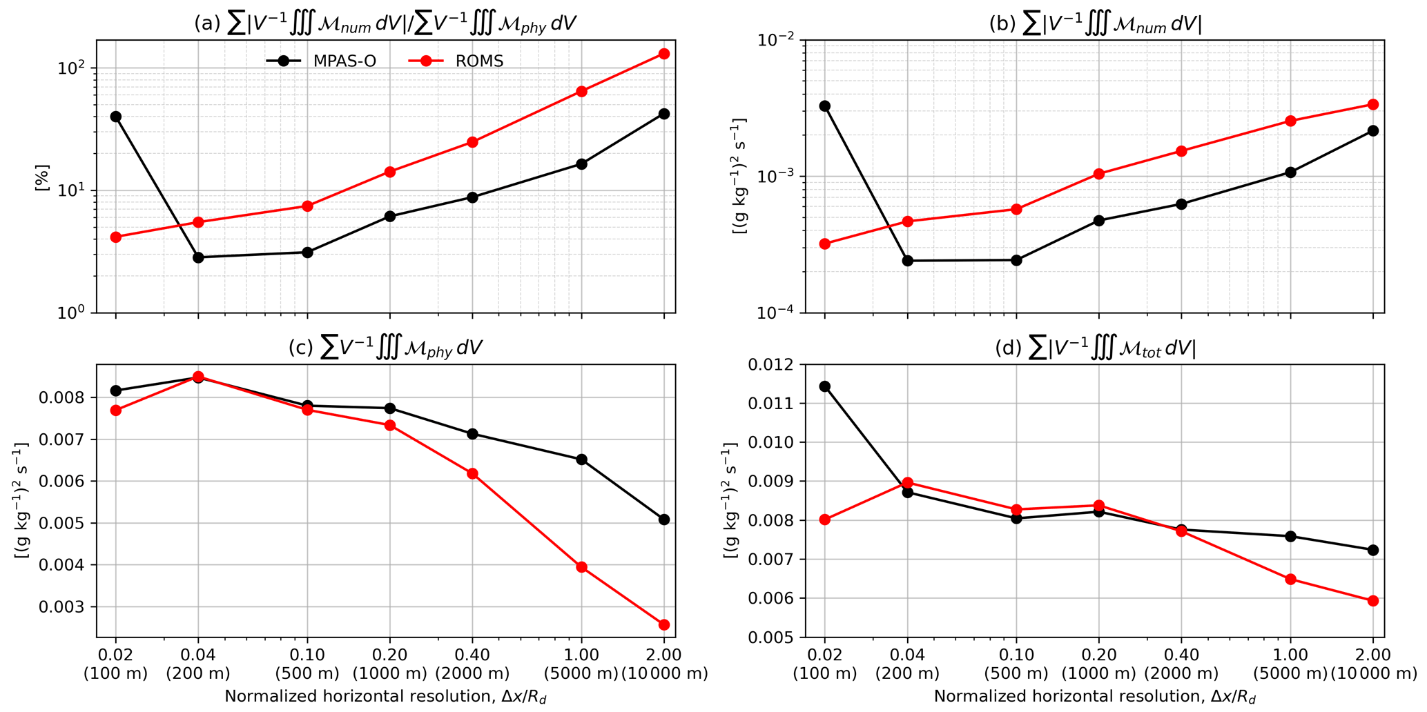
Figure 11 Time-summed volume-averaged mixing as a function of horizontal resolution normalized by the deformation radius (5 km). (a) Bulk ratio of numerical to physical mixing, (b) bulk numerical mixing, (c) bulk physical mixing, and (d) bulk total mixing. Absolute values are used for numerical and total mixing to account for strong variance production in MPAS-O.

As suggested by the time series, bulk numerical mixing in ROMS exceeds MPAS-O at most resolutions. Bulk numerical mixing decreases by 90 % in ROMS from 10 km to 100 m, and by 89 % in MPAS-O from 10 km to 200 m (we exclude the 100 m MPAS-O case due to the massive increase in numerical mixing). Physical mixing increases with resolution in both models: MPAS-O shows a 52 % increase from 10 km to 100 m, while ROMS increases by nearly 200 %. At 5–10 km resolutions, MPAS-O exhibits over 50 % more physical mixing than ROMS, though differences diminish at finer resolutions. Total bulk mixing, defined as $|{\mathcal{M}}_{\mathrm{num}}+{\mathcal{M}}_{\mathrm{phy}}|$, is shown in Fig. 11d. Greater levels of physical mixing in MPAS-O offer a partial explanation as to why there is noticeably less frontal structure than ROMS beyond the halfway point in the simulations. At 5–10 km, ROMS has smaller total mixing than MPAS-O due to lower physical mixing; between 200 m and 2 km, total mixing estimates between both models are within 5 % of each other. For the 100 m MPAS-O simulation, total mixing increases by over 30 % due to the large rise in numerical mixing.

4 Discussion and Conclusions

Two ocean models, MPAS-O and ROMS, with fundamentally different numerical grids and algorithms are found to show similar behavior in the representation of complex frontal dynamics at high spatial resolutions within an idealized configuration of the Mississippi-Atchafalaya River Plume. Statistical metrics of normalized relative vorticity, strain, and divergence confirm that both models quantitatively represent similar scaling of submesoscale processes as horizontal resolution is refined, particularly at the target mid-range resolution of 1 km. Both models demonstrate similar physical dynamics at scales larger than the grid scale that act to increase vertical mixing and restratify the water column, but additional insight can be gained by examining physical invariants (i.e., divergence) at the highest spatial resolutions. Additionally, differences in the asymmetric distribution of relative vorticity and divergence due to spatial resolution are shown to be substantially greater than those due to the choice of ocean model (Fig. 5). These similarities are encouraging because MPAS-O, unlike ROMS, has not been exhaustively tested and tuned in a variety of submesoscale domains.

In this idealized domain, the greatest differences between MPAS-O and ROMS across all resolutions include the timing of baroclinic instability initiation and levels of kinetic energy as well as the peak values in the histogram distributions of relative vorticity and divergence. ROMS attains a higher level of surface kinetic energy approximately 4 d before MPAS-O across all resolutions that is also maintained for a longer period, as baroclinic instabilities across the entirety of the ROMS domain are generated nearly simultaneously (Fig. 3). By contrast, MPAS-O tends to generate these instabilities in a more spatially concentrated area near the center of the domain at mid-range resolutions (i.e., 1 km in data archive animations), and more slowly at higher resolutions than coarser resolutions, resulting in lower average values of surface KE than ROMS earlier in the simulations. Despite differences in the timing of frontogenesis, both models eventually converge to a similar solution (Fig. 3), a feature that is indicative of potential long-term stability for model linkages, particularly for spatial scales that are at the high-fidelity limit of MPAS-O's regional refinement capabilities demonstrated in Part 2.

Another key difference is the decreased structure within and surrounding fronts in MPAS-O during the second half of the simulations. We hypothesize that this is primarily due to the elevated vertical physical salinity mixing in MPAS-O relative to ROMS (Fig. 10), which will accelerate the rate of frontal arrest and decay. These differences in physical mixing are likely because the implementations of the K-profile parameterization differ between models, with MPAS-O using the CVMix library (Van Roekel et al., 2018) and ROMS using its internal KPP scheme. We return to this point again in Part 2.

Differences in momentum advection schemes and the resulting horizontal mixing of momentum are also significant. MPAS-O's second-order centered advection scheme necessitates explicit harmonic and biharmonic dissipation for stability (Ringler et al., 2013), whereas ROMS' third-order upwind scheme provides implicit, flow-adaptive biharmonic dissipation (Shchepetkin and McWilliams, 1998) that only requires a small amount of explicit harmonic viscosity for this domain. This leads to the conundrum where MPAS-O may insufficiently damp grid-scale noise during the frontogenic phase of the simulations and over-damps as the flow relaxes during the frontal arrest and decay phases. ROMS, in contrast, avoids this dilemma because of its flow-adaptive dissipation that effectively suppresses grid scale noise while allowing frontal-scale physical processes to persist longer, evidenced by the release of gravity waves. Shchepetkin and McWilliams (1998) recommend upwinding advection schemes for exactly this reason.

The fairly consistent results earlier in the simulations across multiple resolutions between MPAS-O and ROMS begin to deteriorate for some metrics near the grid scale, with grid scale noise in MPAS-O apparent at resolutions equal to or finer than 500 m. MPAS-O grid scale noise is evident in areas embedded within and adjacent to regions of frontogenesis, and can also be found in regions affected by gravity waves propagating away from the fronts (Fig. 2 and data archive animation). Outside of the frontal regions, ROMS exhibits comparatively lower levels of grid scale noise and numerical noise at fine resolutions, even in the presence of gravity waves released by frontal disequilibrium (Fig. 9m–n). At the finest resolutions (100–200 m), we find more strongly convergent/divergent flow in MPAS-O (Fig. 5e–f) and a wider distribution of along-frontal divergence (Fig. 8d, h). This is almost certainly due to the increased grid-scale noise, which can be identified via physical inspection of the vorticity field (Fig. 2). Our scaling for the biharmonic viscosity was based on a grid Reynolds number of 20, tuned for coarser-resolution fully coupled simulations, but it is insufficient for sub-500 m resolutions. As a simple test (not shown) to ensure the model was not numerically pathological at these resolutions, we reran the 500 m case with double the biharmonic viscosity (grid Reynolds number of 10) and found that it sufficiently reduced grid-scale noise. Rather than tuning biharmonic viscosity for a single parameter space of submesoscale flows, a preferable path forward future work for MPAS-O and Omega is to test flow-adaptive horizontal mixing parameterizations, such as the schemes by Leith (1996) and Smagorinsky (1963)

Tracer advection is also important in differentiating MPAS-O and ROMS at the domain scale through irreversible numerical mixing associated with the different advection schemes (Fig. 10). Our analysis of numerical salinity mixing using the method developed by Burchard and Rennau (2008) demonstrates significant differences between models across all resolutions. MPAS-O generally has less numerical mixing than ROMS when integrated over the domain and summed in time over a simulation (Fig. 11). However, this is not necessarily because the numerical mixing at the grid-scale is weaker in MPAS-O; rather, MPAS-O's flux-corrected transport scheme is less diffusive than the MPDATA scheme used for ROMS. Time series of volume-averaged numerical mixing may oscillate between positive and weakly negative after the frontogenic phase in almost all MPAS-O simulations, implying the effective diffusivity becomes negative. At sub-500 m resolutions, volume-averages of numerical mixing in MPAS-O become more strongly negative, suggesting that the accumulation of kinetic energy and tracer variance at the grid scale may be activating spurious modes in the tracer advection scheme. In fact, this is precisely what is observed for the finest resolution MPAS-O simulation when analyzing the time series of EKE (Fig. 3c). Determining what exactly drives this apparent variance production is therefore a clear direction for future research. Whereas with ROMS, volume-averages of numerical mixing remain positive definite (Fig. 10) and intuitively decrease after peaking during the frontogenic phase. We note that MPDATA is one of several tracer advection schemes available in ROMS, so we expect the relative amount of numerical mixing between models to change if a different advection scheme was used (Kalra et al., 2019; Wang et al., 2021; Schlichting et al., 2024).

This behavior may also provide insight into the results of Petersen et al. (2015), who used volume-integrals of resting potential energy framework to suggest that MPAS-O exhibits less numerical mixing than other ocean models across several idealized test cases. Except in simulations without prescribed physical mixing, the resting potential energy method quantifies the total (physical + numerical) mixing in a model. Strong variance production can drive down bulk estimates of numerical mixing, which are further muddled by using methods that quantify total mixing. Thus, MPAS-O does not necessarily have less numerical mixing than other models.

The submesoscale model comparisons presented here are useful for demonstrating the relative skill of differing numerical approaches when representing small-scale dynamics (particularly for MPAS-O), identifying potential targets for model improvements to specific parameterizations, and providing a pathway for more rigorous model evaluation approaches in realistic domains that have not been previously compared. MPAS-O in particular has been used for mesoscale studies and its expected performance in these smaller, more energetic environments was unclear at the beginning of the study. The overall effect of submesoscale processes in the world's oceans are best answered through modeling efforts, as continuous direct observations of these rapidly evolving and ephemeral flows remain difficult. Additionally, use of numerical models is essential in better understanding fine-scale atmosphere-ocean feedbacks and their impact on global-scale heat transfers. Comparisons of the physical dynamics between structured and unstructured regional ocean models are relatively uncommon, and many published investigations have focused on differences between two commonly used ocean models, ROMS and FVCOM (Chen et al., 2007; Huang et al., 2008). To our knowledge, no comparisons of physical dynamics in existing ocean models have been made against MPAS-O in a regional or idealized context. Constructive comparisons such as this one allow researchers to better determine what dynamics can be simulated by state-of-the-art modeling tools, and provide opportunities for further exploration where models diverge. Additionally, these efforts can help inform decisions regarding the development of training datasets for machine learning approaches, like those that have been previously applied to observations and model outputs for surface dynamics (e.g., Xiao et al., 2023).

The comparable dynamical responses of MPAS-O and ROMS support the hypothesis that these two models similarly represent submesoscale dynamics at multiple similar spatial resolutions, which is of particular interest for research areas that may be under-represented in global models (e.g., coastal domains and open-ocean regions where overturning dynamics play an outsized role in basin-scale circulation patterns). While coupling between the two models will not occur at the same spatial resolution, we can infer from these results that there is unlikely to be a dynamical mismatch at whatever resolution is chosen. A coupled approach would allow for an overall coarser global mesh in MPAS-O that, when coupled to ROMS, may require only a fraction of the increased computational demand necessary for a variable resolution mesh to increase local spatial resolution to submesoscale-permitting resolutions (i.e., ≤ 2 km). Additional challenges that may remain in regionally refining MPAS-O to submesoscale resolution (e.g., representing the distribution of complex bathymetry and river discharge spreading in coastal areas) may be avoided by nesting a high-resolution ROMS model within a global simulation. Increased refinement in the spatial resolution of specific areas can help to build a more complete understanding of critical feedbacks like those associated with freshwater hosing and Atlantic Meridional Overturning Circulation weakening, the departure point and vertical mixing associated with western boundary currents, and net carbon fluxes between highly productive coastal systems and the open ocean. Ongoing and future work will better quantify how this nested approach informs global responses, as well as its strengths and limitations in different ocean regions.

Appendix A: Effects of sloping bathymetry

We configure Bichan at 1 km horizontal resolution with sloping bathymetry to examine how vertical coordinate differences may influence model behavior. All aspects of the configuration are the same as the flat bottom case for 1 km, except variables changed by sloping bathymetry. Because the along-channel velocity is configured in thermal wind balance and our goal is to replicate typical bathymetric gradients found in the nGoM, we configure the bathymetry with two Gaussian depressions with depths ranging from 10 to 75 m (Fig. A1):

$$\begin{array}{}\text{(A1)}& \begin{array}{rl}h(x,y)& =h_s+(h_{\mathrm{d}}-h_{\mathrm{s}})\left[\exp \left(-{\displaystyle \frac{\mathrm{1}}{\mathrm{2}}}{\left({\displaystyle \frac{y-y_{\mathrm{1}}}{\mathit{\sigma }}}\right)}^{\mathrm{2}}\right)\right.\\ & \left.+\exp \left(-{\displaystyle \frac{\mathrm{1}}{\mathrm{2}}}{\left({\displaystyle \frac{y-y_{\mathrm{2}}}{\mathit{\sigma }}}\right)}^{\mathrm{2}}\right)\right],\end{array}\end{array}$$

where h_s=10 m, h_d=75 m, $y_{\mathrm{1}}=\mathrm{7.5}\times {\mathrm{10}}^{\mathrm{4}}$ m, $y_{\mathrm{2}}=\mathrm{1.75}\times {\mathrm{10}}^{\mathrm{5}}$ m, and $\mathit{\sigma }=\mathrm{1.5}\times {\mathrm{10}}^{\mathrm{4}}$ m. This configuration produces a maximum bottom slope of $\partial h/\partial y\sim \mathrm{0.0026}$, roughly twice the mean slope of the nGoM (Hetland, 2017; Zhang et al., 2012).

A uniformly sloping bottom with $\partial h/\partial y=\mathrm{0.001}$ would generate unrealistically strong along-channel velocities (2–3 m s⁻¹) near the northern boundaries based on thermal wind balance. In contrast, using two Gaussian depressions produces localized regions of enhanced depth where the velocity increases with depth, promoting submesoscale activity, while maintaining weaker velocities elsewhere. A single depression with the same minimum depth and slope would leave most of the domain quiescent.

The ROMS vertical grid is configured as a pure sigma coordinate by setting the surface and bottom refinement parameters to zero and the critical depth to 10¹⁶ m. This results in layers ranging from 0.3–2.5 m. In MPAS-O, the vertical grid is configured with the z^* coordinate using partial bottom cells (Pacanowski and Gnanadesikan, 1998) with uniform layer thickness of 2.5 m. The baroclinic timestep for both models is 60 s and the barotropic timestep is 6 s.

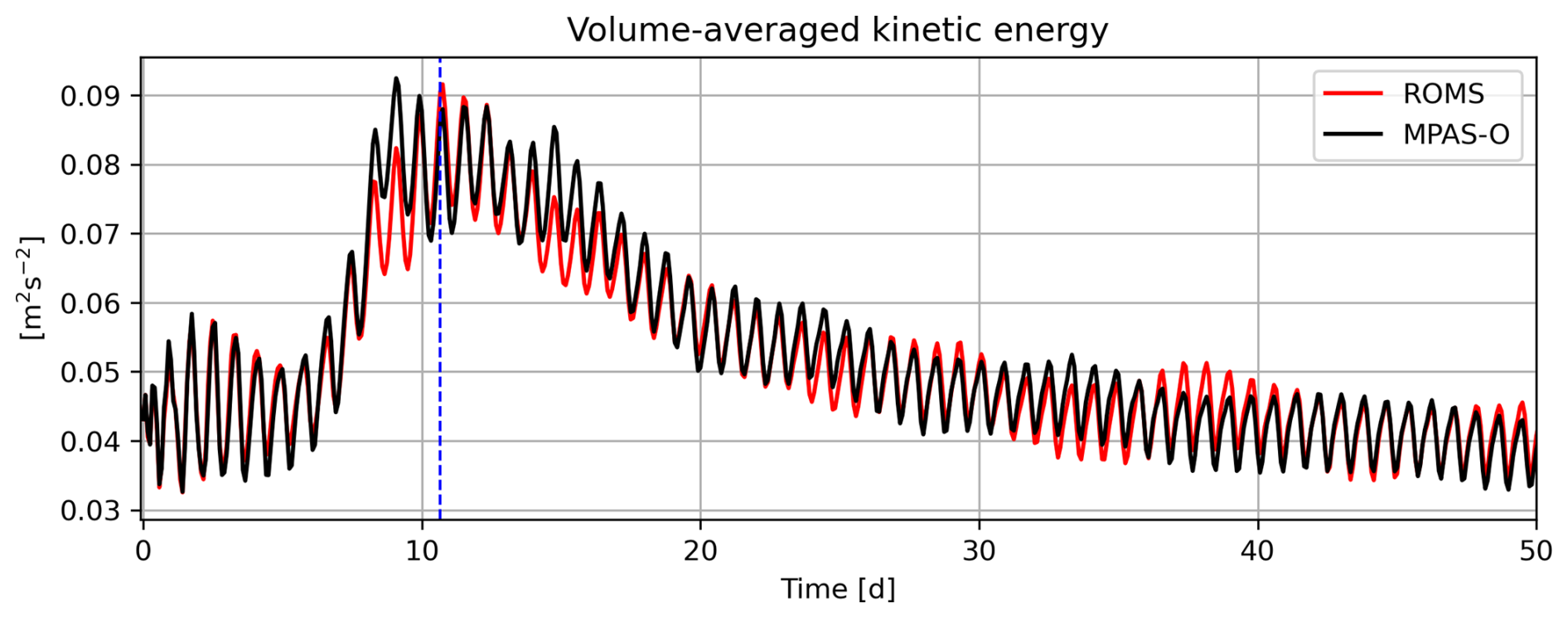
Time series of volume-averaged kinetic energy (Fig. A2) show the development and evolution of eddies in the sloping bathymetry configuration. We use volume-averaged kinetic energy rather than mean surface kinetic energy, as in the flat-bottom case, to capture contributions from the full water column. Eddy formation becomes noticeable around Day 5 in both models, with kinetic energy peaking between Days 8–14. Throughout the simulation, the volume-averaged kinetic energy remains closely matched between MPAS-O and ROMS. Cross-sections of along-channel averaged u velocity during a period of peak kinetic energy (Fig. A1) are also similar, with no indication of spurious mixing or flow impedance from the partial bottom cells. Physically, the vertical shear of u is largely controlled by the lateral density gradient through thermal wind balance. In the deeper regions of the Gaussian depressions – and between them – this produces a weak flow reversal near the bottom. The reversal is slightly stronger in ROMS because it better resolves the near-bottom shear with the terrain-following coordinate.

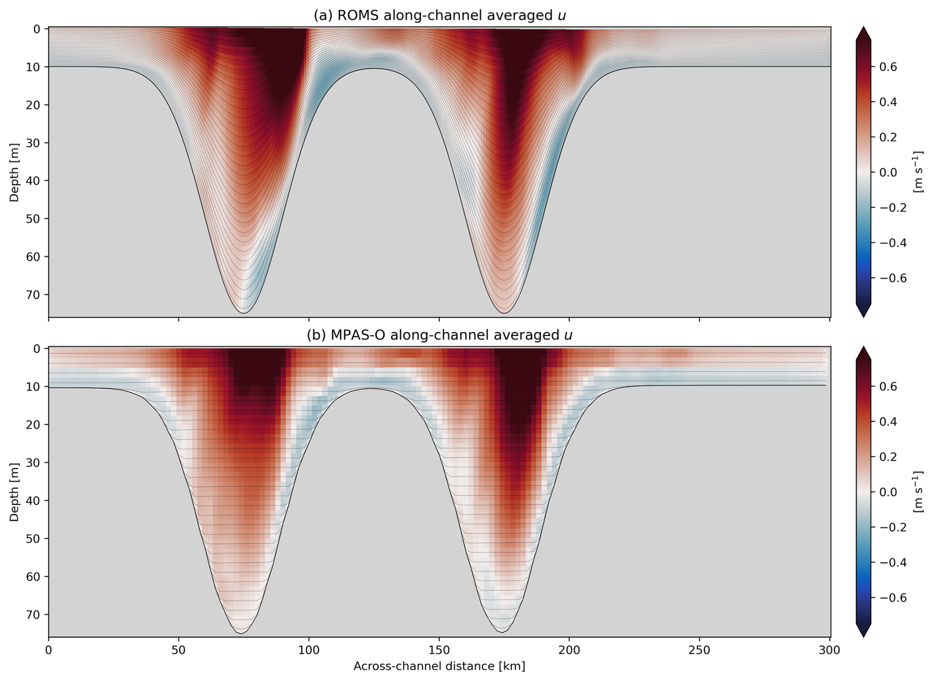
Figure A1 Cross-sections of along-channel averaged u velocity on Day 11 for (a) ROMS and (b) MPAS-O. The thin black lines are the depth of layer centers.

Figure A2 Time series of volume-averaged kinetic energy for the sloping bottom simulations.

Appendix B: Verification of the DVD algorithm

Figure B1 (a) Across-channel-averaged tracer and (b) numerical mixing at t=100 s.

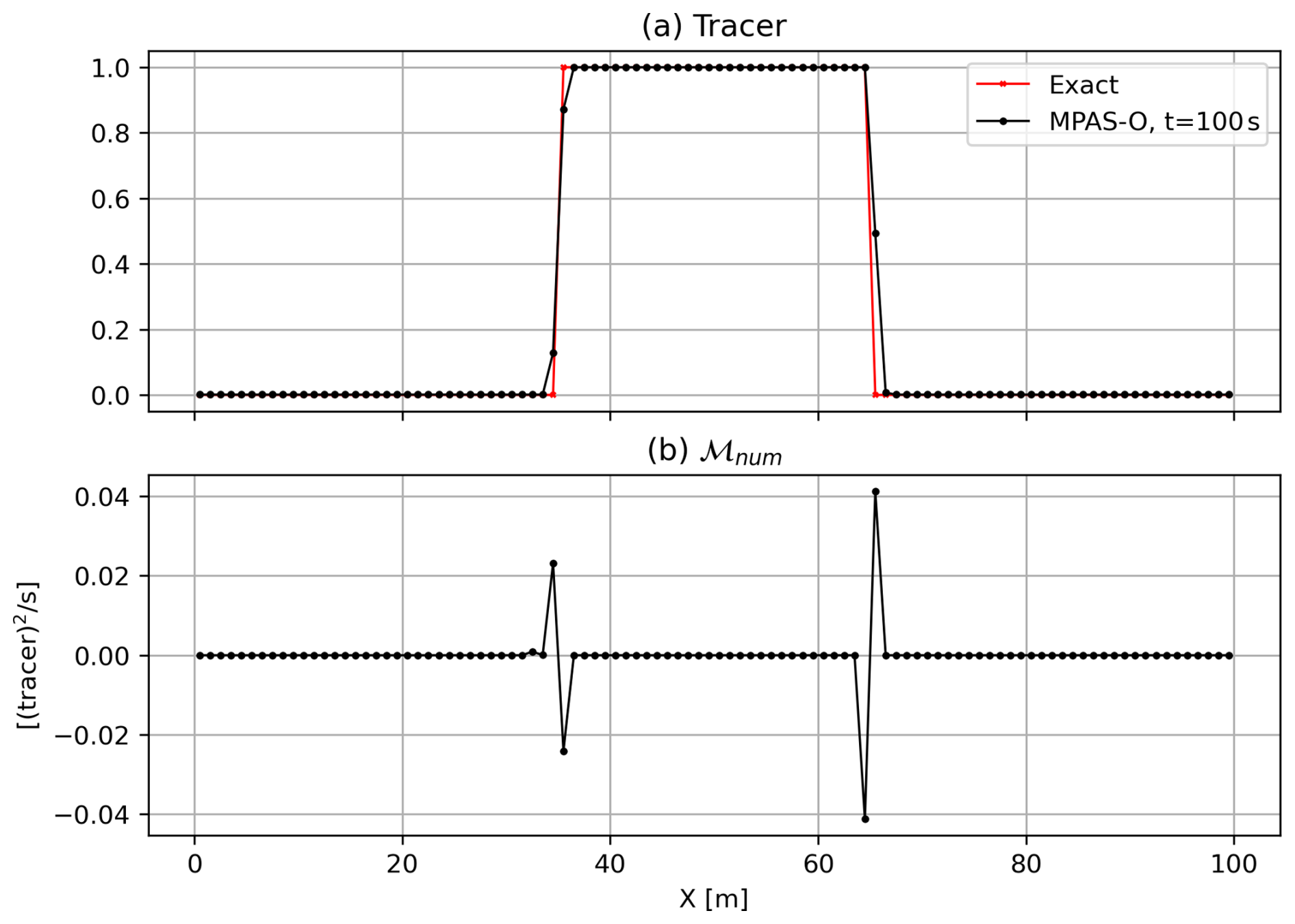
The implementation of the DVD algorithm by Burchard and Rennau (2008) into MPAS-O is verified using a linear advection test. MPAS-O is configured as a single-layer doubly-periodic domain with $L_x=L_y=\mathrm{100}$ m and a water depth of 1 m. The horizontal resolution is Δx=1 m, and the timestep is Δt=0.5 s. Model snapshots are saved at each timestep. The active tracers, denoted by $c(x,y,t)$, are initialized as a top-hat distribution varying only in x:

$$\begin{array}{}\text{(B1)}& {\displaystyle }c(x,y,\mathrm{0}){\displaystyle }=\left\{\begin{array}{ll}\mathrm{1},& \mathrm{35}\le x\le \mathrm{65},\\ \mathrm{0},& \text{otherwise}.\end{array}\right.\end{array}$$

The normal velocity u_n is rotated to be zonally uniform such that ${\mathit{u}}_{\mathrm{n}}=\mathit{u}=\mathrm{1}$ m s⁻¹ and v=0. All momentum and tracer tendencies are disabled except for tracer advection, so the tracer conservation equation reduces to a linear advection equation:

$$\begin{array}{}\text{(B2)}& {\displaystyle \frac{\partial c}{\partial t}}+u{\displaystyle \frac{\partial c}{\partial x}}=\mathrm{0}.\end{array}$$

The analytical solution is

$$\begin{array}{}\text{(B3)}& c(x,y,t)=c\left((x-ut)\mathrm{mod}{L}_x\right).\end{array}$$

Thus, $c(x,y,\mathrm{0})=c(x,y,\mathrm{100})$ analytically, but numerical mixing redistributed the tracer. Figure B1 shows the across-channel-averaged tracer relative to the analytical solution and the corresponding numerical mixing. Positive and negative numerical mixing are observed on both sides of the top-hat. The negative values of numerical mixing result from the flux-corrector, which imposes variance production to enforce monotonicity.

The tracer variance ${c^{\prime }}^{\mathrm{2}}=(c-\stackrel{\mathrm{‾}}{c}{)}^{\mathrm{2}}$, with the volume-averaged tracer $\stackrel{\mathrm{‾}}{c}$, is not conserved due to numerical mixing. Multiplication of Eq. (B3) by 2c^′ yields

$$\begin{array}{}\text{(B4)}& {\displaystyle \frac{\partial {c^{\prime }}^{\mathrm{2}}}{\partial t}}+\mathit{u}{\displaystyle \frac{\partial {c^{\prime }}^{\mathrm{2}}}{\partial x}}=-{\mathcal{M}}_{\mathrm{num}}.\end{array}$$

Volume-integration yields

$$\begin{array}{}\text{(B5)}& \iiint {\displaystyle \frac{\partial {c^{\prime }}^{\mathrm{2}}}{\partial t}}\mathrm{d}V=\iiint -{\mathcal{M}}_{\mathrm{num}}\mathrm{d}V.\end{array}$$

The DVD algorithm can therefore be verified when the volume-integrated variance tendency and the integrated numerical mixing term are equal to machine precision for each timestep, as shown in Fig. B2. The initial strong gradients of the top-hat tracer are smoothed by the flux-corrected transport scheme (Skamarock and Gassmann, 2011). Over 40 timesteps, the volume-integrated variance drops by roughly ten orders of magnitude, at which point the remaining gradients are sufficiently resolved by FCT, and the top hat evolves with minimal smoothing.

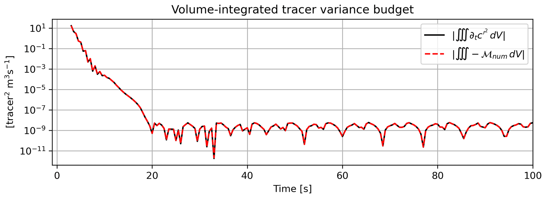
Figure B2 Volume-integrated tracer variance budget for the doubly periodic channel. The first several timesteps are omitted because $\left|{\mathcal{M}}_{\mathrm{num}}\right|$ is undefined at t=0 and to account for the startup transient and two-step lag associated with the second-order Adams-Bashforth time-stepping scheme.