Validating the Nernst–Planck transport model under reaction-driven flow conditions using RetroPy v1.0

Reactive transport processes in natural environments often involve many ionic species. The diffusivities of ionic species vary. Since assigning different diffusivities in the advection–diffusion equation leads to charge imbalance, a single diffusivity is usually used for all species. In this work, we apply the Nernst–Planck equation, which resolves unequal diffusivities of the species in an electroneutral manner, to model reactive transport. To demonstrate the advantages of the Nernst–Planck model, we compare the simulation results of transport under reaction-driven flow conditions using the Nernst–Planck model with those of the commonly used single-diffusivity model. All simulations are also compared to well-defined experiments on the scale of centimeters. Our results show that the Nernst–Planck model is valid and particularly relevant for modeling reactive transport processes with an intricate interplay among diffusion, reaction, electromigration, and density-driven convection.

1 Introduction

Reactive transport processes are fundamental in large-scale subsurface applications such as geological hydrogen storage (Aftab et al., 2022; Hassanpouryouzband et al., 2022), geothermal energy extraction (Randolph and Saar, 2011; Fleming et al., 2020; Ezekiel et al., 2022), biogeochemical subsurface treatments (Carrera et al., 2022), contaminant remediation (Frizon et al., 2003; Reddy and Cameselle, 2009), recovery of minerals (Chang et al., 2021), and carbon sequestration and storage (Luhmann et al., 2013; Tutolo et al., 2014; Pogge von Strandmann et al., 2019; Grimm Lima et al., 2020; Ling et al., 2021). On a smaller scale, reactive transport governs the processes of steel corrosion in reinforced concrete (Yu et al., 2020), cementation processes (Samson and Marchand, 2007; Cochepin et al., 2008), dendrite growth in microelectronics (Illés et al., 2022), and electrochemical reactors (Rivera et al., 2021). In all aforementioned settings, the reacting fluid consists of multiple ionic species and may be subject to an external electric field. In some applications, the electromigration of ionic species can play a significant role in the overall transport process. A typical model that accounts for electromigration is the Nernst–Planck equation.

Modeling electrochemical processes using the Nernst–Planck equation is usually coupled with the Poisson equation for electrical potential, also known as the Poisson–Nernst–Planck (PNP) model. The PNP model has been applied in various electrochemical applications (Jasielec, 2021). In geoscientific applications, benchmarks of the Nernst–Planck model have been proposed and verified considering charged clay surfaces (Tournassat and Steefel, 2021). Charged surfaces affect the water permeability of a porous material (in contrast to air permeability, which is not affected by electric charges) (Revil and Leroy, 2004; Kwon et al., 2004a, b; Cheng and Milsch, 2020). The PNP model is utilized at the pore scale to determine such water permeabilities (Priya et al., 2021). Pore-scale experiments with external charge effects have also been conducted to investigate reactive transport processes (Sprocati et al., 2019; Sprocati and Rolle, 2022; Rolle et al., 2022; Izumoto et al., 2022). Rasouli et al. (2015) verified numerical software using electromigration benchmarks (Lichtner, 1994; Glaus et al., 2013) and multicomponent electromigration experiments considering dispersion effects (Rolle et al., 2013). Finally, multicomponent transport experiments in porous media confirm the validity of the Nernst–Planck model (Muniruzzaman et al., 2014; Muniruzzaman and Rolle, 2015, 2017; Rolle et al., 2018).

The above benchmark and validation studies focused on reactions and the mixing of fluids, which are subject to flow introduced by fluid pressure or electric fields. In this work, we propose another set of benchmark problems for numerical models, based on chemically driven convection experiments (Avnir and Kagan, 1984; Eckert and Grahn, 1999; Eckert et al., 2004), which focus on how reaction and mixing of fluids influence fluid flow. The concept of reaction-driven flow is as follows: consider reaction $A+B\to C$, where A and B are the reactants and C is the product. If A, B, and C have different material properties, for example, viscosity, diffusivity, and/or density, the reaction can induce fluid flow and hydrodynamic instabilities in such systems (De Wit, 2016, 2020). We are interested in aqueous systems, where ionic species exist, such that the Nernst–Planck model is applicable.

Zalts et al. (2008) performed experiments using an acid and a base to study chemically driven convection. Related experiments and theories of the underlying mechanism have emerged: unequal species diffusivities (Citri et al., 1990; Almarcha et al., 2010, 2011; Trevelyan et al., 2011; Lemaigre et al., 2013; Kim, 2019; Jotkar et al., 2021), the same species diffusivity but with varying viscosity (Hejazi and Azaiez, 2013), and concentration-dependent species diffusivities (Bratsun et al., 2015, 2017, 2021, 2022). Chemically driven convection has also been investigated using a weak acid and a weak base (Cherezov et al., 2018). Since the Nernst–Planck model is expected to be able to account for unequal species diffusivities and has the characteristics of concentration-dependent diffusive fluxes, we examine the validity of the Nernst–Planck model by comparing our Nernst–Planck simulations with chemically driven experiments conducted by others.

In addition, we present simulations of convective dissolution of CO₂, a process which is important in the underground storage of CO₂ (Singh et al., 2019). Thomas et al. (2016) performed experiments of convective dissolution of CO₂ into alkaline brines, including LiOH and NaOH, and observed that different cations lead to varying onset times and fingering patterns. Thomas et al. (2016) proposed that the inert cation, which does not participate in the acid–base reaction between the dissolved CO₂ and the brine, plays a major role in the development of convective instabilities. Since dissolved CO₂ forms charged and uncharged states (CO₂(aq), ${\mathrm{HCO}}_{\mathrm{3}}^{-}$, ${\mathrm{CO}}_{\mathrm{3}}^{\mathrm{2}-}$) when the pH changes as a consequence of neutralization reactions, it is natural to apply the Nernst–Planck model in such cases.

In the following sections, we first establish the fundamental equations of the conservation laws and the accompanying numerical methods. We then provide details concerning the two reaction-driven flow experiments and a CO₂ dissolution experiment – all conducted by others. We compare the differences between the simulations of the single-diffusivity transport model and the Nernst–Planck model and elucidate the necessity of considering electromigration effects caused by differing diffusivities during reactive transport modeling.

2 Materials and methods

2.1 Fundamental equations for reactive transport processes

In this section, we delineate the fundamental equations describing the reactive transport of aqueous species.

2.1.1 Mass balance of the fluid components

We consider a single-phase fluid composed of N components, which can be ionic species, dissolved gas, or minerals. The single-phase fluid occupies a certain volume V_f, and the ith component of the fluid has the mass m_i. The mass concentration of the ith component is defined as

$$\begin{array}{}\text{(1)}& {\mathit{\rho }}_i={\displaystyle \frac{m_i}{V_{\mathrm{f}}}}.\end{array}$$

We use the term mass concentration to clarify that ρ_i is not the density of the component. The fluid density, ρ, can be obtained by summing up the mass concentrations of the components, i.e.,

$$\begin{array}{}\text{(2)}& \mathit{\rho }=\sum _{i=\mathrm{1}}^N{\mathit{\rho }}_i=\sum _{i=\mathrm{1}}^N{\displaystyle \frac{m_i}{V_{\mathrm{f}}}}.\end{array}$$

In general, the fluid density is a function of fluid pressure, p; temperature, T; and fluid composition (i.e., the mass concentrations, ρ_i). The equation of state of the fluid density can be written as

$$\begin{array}{}\text{(3)}& \mathit{\rho }=\mathit{\rho }(p,T,{\mathit{\rho }}_i;i=\mathrm{1},\mathrm{2},\mathrm{\dots },N).\end{array}$$

The mass balance of each fluid component is described by the continuity equation,

$$\begin{array}{}\text{(4)}& {\displaystyle \frac{\partial {\mathit{\rho }}_i}{\partial t}}+\mathrm{\nabla }\cdot \left({\mathit{\rho }}_i{\mathit{v}}_i\right)=Q_i,\end{array}$$

where ρ_iv_i is the mass flux and Q_i is the source or sink term introduced by chemical reactions. Since chemical reactions preserve fluid mass, we have ${\sum }_i{Q}_i=\mathrm{0}$. We express the mass flux of the ith component as

$$\begin{array}{}\text{(5)}& {\mathit{\rho }}_i{\mathit{v}}_i={\mathit{\rho }}_i\mathit{u}+{\mathit{\rho }}_i{\mathit{u}}_{\mathrm{EP},i}+{\mathit{J}}_{\mathrm{diff},i},\end{array}$$

where u is the barycentric velocity, u_EP,i is the electrophoretic velocity, and J_diff,i is the diffusive flux. In the following sections, we define the models of the diffusive flux, the electrophoretic flux, and the barycentric flux.

2.1.2 Modeling of the diffusive flux

We use standard Fickian diffusion to model the diffusive flux,

$$\begin{array}{}\text{(6)}& {\mathit{J}}_{\mathrm{diff},i}=-D_i{M}_i\mathrm{\nabla }{C}_{i}i=\mathrm{1},\mathrm{2},\mathrm{\dots },N-\mathrm{1},\end{array}$$

where D is the diffusivity, M is the molar mass, and C is the molar concentration. The contribution of the diffusing solvent can be neglected, considering ${\mathit{\rho }}_i/{\mathit{\rho }}_N\ll \mathrm{1}$. Such an assumption leads to a particular choice of the Nth component, which contributes the most mass to the fluid. In our experiments of interest, the Nth component is H₂O(l). Fickian diffusion utilizes the diagonal diffusivity matrix assumption, which is valid for many electrolytes (Dreyer et al., 2013). A diagonal diffusivity matrix means that short-range interactions between ions are negligible, which restricts our model to dilute solutions (Kontturi et al., 2008).

2.1.3 Modeling of the barycentric flux

The type of experiments of interest for this work is performed in a Hele-Shaw cell, for which fluid flow can be described by Darcy's law,

$$\begin{array}{}\text{(7)}& \mathit{u}=-{\displaystyle \frac{k}{\mathit{\eta }}}\left(\mathrm{\nabla }p-\mathit{\rho }\mathit{g}\right),\end{array}$$

where k is the permeability, η is the dynamic viscosity of the fluid, and g is the gravitational acceleration. When combined with the incompressibility assumption,

$$\begin{array}{}\text{(8)}& \mathrm{\nabla }\cdot \left(\mathit{\rho }\mathit{u}\right)=\mathrm{0},\end{array}$$

u and p can be obtained. The scalar permeability of a Hele-Shaw cell, with a gap width of w, is given by

$$\begin{array}{}\text{(9)}& k={\displaystyle \frac{w^{\mathrm{2}}}{\mathrm{12}}}.\end{array}$$

2.1.4 Modeling of the electrophoretic flux

When the components in the fluids are electrically charged, for example, the ions Na⁺ or Cl⁻, we have to consider the effect of Coulombic forces among the ions. Such Coulombic forces are typically modeled by incorporating the electric field E into the mass fluxes of the fluid components (Boudreau et al., 2004). The electrophoretic flux is described by

$$\begin{array}{}\text{(10)}& {\mathit{\rho }}_i{\mathit{u}}_{\mathrm{EP},i}={\displaystyle \frac{z_i{\mathit{\rho }}_i{D}_{i}F}{RT}}\mathit{E},\end{array}$$

where z_i is the charge number of the fluid component, F is the Faraday constant, R is the ideal gas constant, and T is the fluid temperature. We require the charge conservation equation to define the electric field in a multicomponent fluid. To obtain the charge conservation equation of the ionic species, it is useful to use the flux defined in molar concentration. Using ρ_i=M_iC_i, we have the mass conservation equation (without considering the source or sink terms introduced by reactions)

$$\begin{array}{}\text{(11)}& {\displaystyle \frac{\partial C_i}{\partial t}}=-\mathrm{\nabla }\cdot (C_i\mathit{u}+C_i{\mathit{u}}_{\mathrm{EP},i}+{\mathit{J}}_{\mathrm{diff},i}/M_i).\end{array}$$

Following the derivations of Kirby (2010), the charge density is defined as

$$\begin{array}{}\text{(12)}& {\mathit{\rho }}_{\mathrm{E}}=F\sum _{i=\mathrm{1}}^{N-\mathrm{1}}{z}_i{C}_i.\end{array}$$

The charge conservation equation is the sum of Eq. (11) over all ionic species multiplied by the charge number and the Faraday constant,

$$\begin{array}{}\text{(13)}& {\displaystyle \frac{\partial {\mathit{\rho }}_{\mathrm{E}}}{\partial t}}=-F\mathrm{\nabla }\cdot \left(\sum _{i=\mathrm{1}}^{N-\mathrm{1}}{z}_i{C}_i\mathit{u}+z_i{C}_i{\mathit{u}}_{\mathrm{EP},i}+z_i{\mathit{J}}_{\mathrm{diff},i}/M_i\right).\end{array}$$

We assume the aqueous solution is locally electroneutral,

$$\begin{array}{}\text{(14)}& \sum _{i=\mathrm{1}}^{N-\mathrm{1}}{z}_i{C}_i=\mathrm{0},\end{array}$$

which is an approximation considering the Debye length (typically on the order of nanometers) vanishes at the length scale of the considered system (Dickinson et al., 2011). The electroneutrality assumption eliminates the barycentric flux term in the charge conservation equation. We consider Fickian diffusive flux, Eq. (6), and the electrophoretic flux, Eq. (10), so that the charge conservation is given by

$$\begin{array}{}\text{(15)}& {\displaystyle \frac{\partial {\mathit{\rho }}_{\mathrm{E}}}{\partial t}}=-\mathrm{\nabla }\cdot \left(\sum _{i=\mathrm{1}}^{N-\mathrm{1}}{\displaystyle \frac{D_i{C}_i(z_{i}F{)}^{\mathrm{2}}}{RT}}\mathit{E}-\sum _{i=\mathrm{1}}^{N-\mathrm{1}}{D}_i{z}_{i}F\mathrm{\nabla }{C}_i\right).\end{array}$$

The multiplier of the electric field, E, is the electrical conductivity (${\mathrm{C}}^{\mathrm{2}}{\mathrm{m}}^{-\mathrm{3}}{\mathrm{kg}}^{-\mathrm{1}}\mathrm{s}$),

$$\begin{array}{}\text{(16)}& \mathit{\sigma }=\sum _{i=\mathrm{1}}^{N-\mathrm{1}}{\displaystyle \frac{D_i{C}_i(z_{i}F{)}^{\mathrm{2}}}{RT}}.\end{array}$$

When the diffusivities of all species are equal, D_i=D, the diffusive flux in the charge conservation equation is

$$\begin{array}{}\text{(17)}& D\sum _{i=\mathrm{1}}^{N-\mathrm{1}}{z}_{i}F\mathrm{\nabla }{C}_i=D\mathrm{\nabla }\left(F\sum _{i=\mathrm{1}}^{N-\mathrm{1}}{z}_i{C}_i\right)=\mathrm{0}.\end{array}$$

Then, the charge conservation equation yields Laplace's equation of the electric potential, i.e., $\mathrm{\nabla }\cdot \left(\mathit{\sigma }\mathrm{\nabla }\mathit{\varphi }\right)=\mathrm{0}$, where $\mathit{E}=-\mathrm{\nabla }\mathit{\varphi }$. However, the diffusivity of the chemical species varies with molecular size and can differ by up to an order of magnitude. Such variations in molecular diffusivity lead to diffusive fluxes that produce an electric field. The model that combines mass conservation, Eq. (11), and Poisson's equation of electrostatics, is known as the Poisson–Nernst–Planck (PNP) model (Pamukcu, 2009).

The PNP model aims at resolving both the electric potential and the molar concentrations subject to the boundary conditions of the electric potential. The mathematical properties of the PNP model, with no external flow (Filipek et al., 2017), coupled with Darcy flow (Herz et al., 2012; Ignatova and Shu, 2022), and coupled with Navier–Stokes flow (Lee, 2021; Constantin et al., 2021, 2022) are still being explored. Rigorous upscaling and homogenization of the PNP–Stokes system has been performed (Ray et al., 2012a; Kovtunenko and Zubkova, 2021), and the upscaled formulations are examined by numerical modeling (Frank et al., 2011; Ray et al., 2012b). Numerical methods and solution techniques of the PNP equations are an ongoing research field (Flavell et al., 2014; Song et al., 2018; Shen and Xu, 2021; Liu and Maimaitiyiming, 2021; Yan et al., 2021; Liu et al., 2022; Zhang et al., 2022). Models similar to the PNP model also arise in modeling multicomponent interdiffusion of solids (Bożek et al., 2019), where the experimental comparison and the development of numerical methods are studied by Sapa et al. (2020) and Bożek et al. (2021).

In this work, we enforce the null current condition

$$\begin{array}{}\text{(18)}& \sum _{i=\mathrm{1}}^{N-\mathrm{1}}{\displaystyle \frac{D_i{C}_i(z_{i}F{)}^{\mathrm{2}}}{RT}}\mathit{E}-\sum _{i=\mathrm{1}}^{N-\mathrm{1}}{D}_i{z}_{i}F\mathrm{\nabla }{C}_i=\mathrm{0},\end{array}$$

to ensure that no charge accumulates at the continuum scale of interest,

$$\begin{array}{}\text{(19)}& {\displaystyle \frac{\partial {\mathit{\rho }}_{\mathrm{E}}}{\partial t}}=\mathrm{0}.\end{array}$$

This result is a simplification of the PNP model. The null current condition has been utilized in modeling multicomponent ionic transport (Lichtner, 1985; Cappellen and Gaillard, 1996; Giambalvo et al., 2002; Muniruzzaman and Rolle, 2019; Cogorno et al., 2022; López-Vizcaíno et al., 2022). The combined assumptions of local electroneutrality and null current are referred to as strict electroneutrality by Lees et al. (2017). Furthermore, if there are no sources of the electric field (Tabrizinejadas et al., 2021), then the electric field can be represented by

$$\begin{array}{}\text{(20)}& \mathit{E}={\displaystyle \frac{RT}{F}}{\displaystyle \frac{{\sum }_{j=\mathrm{1}}^{N-\mathrm{1}}{D}_j{z}_j\mathrm{\nabla }{C}_j}{{\sum }_{k=\mathrm{1}}^{N-\mathrm{1}}(z_k{)}^{\mathrm{2}}{D}_k{C}_k}},\end{array}$$

where we use j and k as summation indices. Hence, the molar electrophoretic flux of individual species can be formulated as

$$\begin{array}{}\text{(21)}& C_i{\mathit{u}}_{\mathrm{EP},i}={\displaystyle \frac{z_i{D}_i{C}_{i}F}{RT}}\mathit{E}=z_i{D}_i{C}_i{\displaystyle \frac{{\sum }_{j=\mathrm{1}}^{N-\mathrm{1}}{z}_j{D}_j\mathrm{\nabla }{C}_j}{{\sum }_{k=\mathrm{1}}^{N-\mathrm{1}}(z_k{)}^{\mathrm{2}}{D}_k{C}_k}}.\end{array}$$

There are many physical interpretations of such a flux. For example, one is that the dissolved species is advecting due to the electric field. Another point of view can be obtained by combining Eq. (21) with the Fickian diffusion flux,

$$\begin{array}{ll}{\displaystyle }& {\displaystyle }{\mathit{J}}_{\mathrm{diff},i}/M_i+C_i{\mathit{u}}_{\mathrm{EP},i}\\ \text{(22)}& {\displaystyle }& {\displaystyle }=-D_i\mathrm{\nabla }{C}_i+{\displaystyle \frac{z_i{D}_i{C}_i}{{\sum }_{k=\mathrm{1}}^{N-\mathrm{1}}(z_k{)}^{\mathrm{2}}{D}_k{C}_k}}\sum _{j=\mathrm{1}}^{N-\mathrm{1}}{z}_j{D}_j\mathrm{\nabla }{C}_j\text{(23)}& {\displaystyle }& {\displaystyle }=-\sum _{j=\mathrm{1}}^{N-\mathrm{1}}{D}_{ij}\mathrm{\nabla }{C}_j,\end{array}$$

which corresponds to the “natural generalization” of Fickian diffusion, denoted by Onsager (1945). Following Boudreau et al. (2004), the cross-coupling diffusivities are given by

$$\begin{array}{}\text{(24)}& \begin{array}{rl}{D}_{ij}& ={\mathit{\delta }}_{ij}{D}_i-{\displaystyle \frac{z_i{z}_j{D}_i{D}_j{C}_i}{{\sum }_{k=\mathrm{1}}^{N-\mathrm{1}}(z_k{)}^{\mathrm{2}}{D}_k{C}_k}}\\ & ={\mathit{\delta }}_{ij}{D}_i-{\displaystyle \frac{z_i{D}_i{C}_i\otimes z_j{D}_j}{{\sum }_{k=\mathrm{1}}^{N-\mathrm{1}}(z_k{)}^{\mathrm{2}}{D}_k{C}_k}},\end{array}\end{array}$$

where Einstein's summation convention is not applied. Hence, locally electroneutral diffusion is equivalent to nonlinear multicomponent diffusion with a diffusivity tensor being a rational function of molar concentrations of the charged species (Rubinstein, 1990). Similar forms of the cross-coupling diffusivities can also be found in Lichtner (1985).

Combining Eqs. (11) and (22) yields

$$\begin{array}{}\text{(25)}& {\displaystyle \frac{\partial C_i}{\partial t}}=-\mathrm{\nabla }\cdot \left(-D_i\mathrm{\nabla }{C}_i+z_i{D}_i{C}_i{\displaystyle \frac{{\sum }_{j=\mathrm{1}}^{N-\mathrm{1}}{z}_j{D}_j\mathrm{\nabla }{C}_j}{{\sum }_{k=\mathrm{1}}^{N-\mathrm{1}}(z_k{)}^{\mathrm{2}}{D}_k{C}_k}}+\mathit{u}{C}_i\right),\end{array}$$

which is the Nernst–Planck equation for single-phase multicomponent systems. If all species have the same diffusivity, D_i=D, and the aqueous solution is electroneutral, Eq. (14) is used. Then, the single-phase multicomponent Nernst–Planck equation reduces to

$$\begin{array}{}\text{(26)}& {\displaystyle \frac{\partial C_i}{\partial t}}=-\mathrm{\nabla }\cdot \left(-D\mathrm{\nabla }{C}_i+\mathit{u}{C}_i\right),\end{array}$$

which we refer to as the single-diffusivity model. Both the Nernst–Planck model and the single-diffusivity model satisfy the electroneutrality condition, Eq. (14), and the zero-charge accumulation assumptions, Eq. (19). However, of the two models, only the Nernst–Planck model is capable of handling the physics of varying species diffusivities. To communicate the effectiveness of the Nernst–Planck equation in reactive transport scenarios, we compare the modeling results with the single-diffusivity model, which is a common approach. We set the diffusivity of the single-diffusivity model as $\mathrm{3}\times {\mathrm{10}}^{-\mathrm{3}}$ mm² s⁻¹, which is within the common values for species diffusivities in water at 25 ^∘C.

2.1.5 Chemical equilibrium using Gibbs energy minimization

Another aspect of mass balance amongst the fluid components, which we now denote as the chemical species, is the reaction that changes the amount of the chemical species while conserving the mass balance of chemical elements. The reaction source or sink term in the mass balance of each fluid component, Q_i, is implicitly formulated as the Gibbs energy minimization problem,

$$\begin{array}{}\text{(27)}& \begin{array}{rl}& \underset{n}{min}G=\sum _{i=\mathrm{1}}^N{\mathrm{n}}_i{\mathit{\mu }}_i\\ & \text{subject to }\left\{\begin{array}{l}\text{mass balance of chemical elements}\\ \mathrm{n}\ge \mathrm{0}\end{array}\right.,\end{array}\end{array}$$

where G is the Gibbs energy and n_i is the molar amount of the ith chemical species. The chemical potential is defined as

$$\begin{array}{}\text{(28)}& {\mathit{\mu }}_i={\mathit{\mu }}_i^{\circ }+RT\log a_i,\end{array}$$

where ${\mathit{\mu }}_i^{\circ }$ is the standard chemical potential of the ith species and a_i is the activity of the ith species. For the standard chemical potential, we employ the SUPCRT07 database (Johnson et al., 1992). To evaluate the activities, we use the Helgeson–Kirkham–Flowers (HKF) activity model (Helgeson and Kirkham, 1974a, b, 1976; Helgeson et al., 1981), which is based on the extended Debye–Hückel activity model. For the activity model of CO₂(aq), we use the Drummond model (Drummond, 1981). The combination of the SUPCRT database and the HKF activity model is utilized in many geochemical modeling packages, such as EQ3/6 (Wolery, 1992), CHILLER (Reed, 1998), ChemApp (Petersen and Hack, 2007), Perplex (Connolly, 2009), GEM-Selektor (Kulik et al., 2012), PHREEQC (Parkhurst and Appelo, 2013), Geochemist's Workbench (Bethke, 2007), and Reaktoro (Leal, 2022) (Miron et al., 2019). General reviews of the activity models can be found in Marini (2007) and Hingerl (2012).

We use Reaktoro to solve the chemical equilibrium problem. The numerical methods and implementations of the Gibbs energy minimization problem are detailed in Leal et al. (2014, 2016, 2017). The equilibrium calculations are performed at every time step and for every discretized volume of the simulation domain, and calculations of similar chemical states can be cached for efficiency. Efficient lookup tables and machine learning approaches of chemical-equilibrium calculations are in active research (Huang et al., 2018; De Lucia and Kühn, 2021; De Lucia et al., 2021; Savino et al., 2022; Laloy and Jacques, 2022), and significant speedups in solving reactive transport problems have been achieved (Kyas et al., 2022; Bordeaux-Rego et al., 2022). In particular, Reaktoro employs on-demand machine learning and physics-based interpolation, which is able to conserve mass and control interpolation accuracy (Leal et al., 2020). Surrogate models of the full reactive transport process using machine learning have also been developed (Sprocati and Rolle, 2021). However, to avoid approximation errors, machine learning approaches and surrogate models are not employed in this work.

2.2 Numerical schemes

This section elaborates on the numerical schemes we use for solving the fundamental equations of the reactive transport processes.

2.2.1 The barycentric flux

We utilize the mixed finite-element formulation to solve for fluid velocity and fluid pressure under the constraints of mass balance, Eq. (8), and momentum balance, Eq. (7). To avoid spurious solutions, the finite-element spaces have to satisfy the Ladyzhenskaya–Babuška–Brezzi (LBB) condition. We refer the reader to other works for further discussions regarding the LBB condition in the context of fluid flow problems (Donea and Huerta, 2003), geodynamics (Thieulot and Bangerth, 2022), and elasticity and electromagnetic applications (Boffi et al., 2013). We select LBB-compatible elements, namely the zeroth-order Raviart–Thomas (RT) element for the barycentric flux and the piecewise constant element for the pressure (Raviart and Thomas, 1977). Another popular LBB-compatible element is the Brezzi–Douglas–Marini element (Brezzi et al., 1985). The mixed finite-element formulation can be written in matrix form as

$$\begin{array}{}\text{(29)}& \left(\begin{array}{cc}\mathbf{A}& {\mathbf{B}}^T\\ \mathbf{B}& \mathrm{0}\end{array}\right)\left[\begin{array}{c}\widehat{\mathit{u}}\\ \widehat{\mathit{p}}\end{array}\right]=\left[\begin{array}{c}\mathit{f}\\ \mathrm{0}\end{array}\right],\end{array}$$

where $\widehat{\mathit{u}}$ and $\widehat{\mathit{p}}$ are the solution vectors for the barycentric velocity and the fluid pressure. Such a formulation leads to a saddle point problem. Following Benzi et al. (2005)'s review of saddle point problems, one can apply Uzawa's method (Uzawa, 1958) to solve such problems. Given an initial condition of ${\widehat{\mathit{p}}}^n$ at step n, Uzawa's method solves $\widehat{\mathit{u}}$ and $\widehat{\mathit{p}}$ iteratively,

$$\begin{array}{}\text{(30)}& {\displaystyle }{\widehat{\mathit{u}}}^{n+\mathrm{1}}={\mathbf{A}}^{-\mathrm{1}}(\mathit{f}-{\mathbf{B}}^T{\widehat{\mathit{p}}}^n),\text{(31)}& {\displaystyle }{\widehat{\mathit{p}}}^{n+\mathrm{1}}={\widehat{\mathit{p}}}^n+\mathit{\omega }\mathbf{B}{\widehat{\mathit{u}}}^{n+\mathrm{1}},\end{array}$$

where ω>0 is a relaxation parameter. Normally, Uzawa's method converges slowly and requires many iterations, meaning that improving Uzawa's method is an ongoing research effort (Bacuta, 2006). We use one of the improved methods, the augmented Lagrangian Uzawa's method, introduced by Fortin and Glowinski (1983):

$$\begin{array}{}\text{(32)}& \left(\begin{array}{cc}\mathbf{A}+r{\mathbf{B}}^T\mathbf{B}& {\mathbf{B}}^T\\ \mathbf{B}& \mathrm{0}\end{array}\right)\left[\begin{array}{c}\widehat{\mathit{u}}\\ \widehat{\mathit{p}}\end{array}\right]=\left[\begin{array}{c}\mathit{f}\\ \mathrm{0}\end{array}\right],\end{array}$$

where r>0 is a tuning parameter. We solve the matrix problem iteratively,

$$\begin{array}{}\text{(33)}& {\displaystyle }{\widehat{\mathit{u}}}^{n+\mathrm{1}}=(\mathbf{A}+r{\mathbf{B}}^T\mathbf{B}{)}^{-\mathrm{1}}(\mathit{f}-{\mathbf{B}}^T{\widehat{\mathit{p}}}^n),\text{(34)}& {\displaystyle }{\widehat{\mathit{p}}}^{n+\mathrm{1}}={\widehat{\mathit{p}}}^n+\mathit{\omega }\mathbf{B}{\widehat{\mathit{u}}}^{n+\mathrm{1}}.\end{array}$$

When ω=r, we can choose sufficiently large r to accelerate the convergence of Uzawa's method. However, the matrix A+rB^TB becomes more ill-conditioned as r increases, which may lead to a large number of iterations to solve when applying an iterative method (Fortin and Glowinski, 1983). Hence, we use the MUMPS (Amestoy et al., 2001, 2019) direct solver to update the velocity, Eq. (33). The degrees of freedom of $\widehat{\mathit{u}}$ in our simulations range from 17 000 to 140 000.

2.2.2 Transport of fluid components

In the previous section, we selected an LBB-compatible velocity and pressure pair. The basis function of pressure is a piecewise constant, which can be described as the average pressure of a certain cell volume in a given mesh. Therefore, it is straightforward to define the molar concentrations as piecewise constants. We use the finite-volume method to discretize the transport of the fluid components, Eq. (25):

$$\begin{array}{}\text{(35)}& \begin{array}{rl}\underset{\mathrm{\Omega }}{\int }{q}_i{\displaystyle \frac{\partial C_i}{\partial t}}\mathrm{d}\mathrm{\Omega }& =-\underset{\mathrm{\Gamma }}{\int }{q}_i(-D_i\mathrm{\nabla }{C}_i\\ & +z_i{D}_i{C}_i{\displaystyle \frac{{\sum }_{j=\mathrm{1}}^{N-\mathrm{1}}{z}_j{D}_j\mathrm{\nabla }{C}_j}{{\sum }_{k=\mathrm{1}}^{N-\mathrm{1}}(z_k{)}^{\mathrm{2}}{D}_k{C}_k}}+\mathit{u}{C}_i)\cdot \mathit{n}\mathrm{d}\mathrm{\Gamma },\end{array}\end{array}$$

where the fluxes are yet to be defined. Considering no-flux boundary conditions of the fluid components, we use the two-point flux approximation scheme (TPFA) for the diffusive flux,

$$\begin{array}{}\text{(36)}& \underset{\mathrm{\Gamma }}{\int }{q}_i{D}_i\mathrm{\nabla }{C}_i\cdot \mathit{n}\mathrm{d}\mathrm{\Gamma }=-\underset{{\mathrm{\Gamma }}_{\mathrm{int}}}{\int }\left[q_i\right]D_i{\displaystyle \frac{\left[C_i\right]}{h}}\mathrm{d}\mathrm{\Gamma },\end{array}$$

where Γ_int denotes the interior cell interfaces, [•] is the jump operator that evaluates the difference in a function across a common interface of two cells, and h is the distance between the cell centers. We assumed that the diffusivity of each species is constant. For diffusivities varying in space, Tournassat et al. (2020) discussed and compared various averaging approaches of the diffusivities at the interfaces between cells. For the advective flux, we utilize the full upwinding method,

$$\begin{array}{}\text{(37)}& -\underset{\mathrm{\Gamma }}{\int }{q}_i{C}_i\mathit{u}\cdot \mathit{n}\mathrm{d}\mathrm{\Gamma }=-\underset{{\mathrm{\Gamma }}_{\mathrm{int}}}{\int }\left[q_i\right]C_i^{\mathrm{up}}\mathit{u}\cdot \mathit{n}\mathrm{d}\mathrm{\Gamma },\end{array}$$

where $C_i^{\mathrm{up}}$ is the molar concentration in the upwind direction. For the Nernst–Planck term, we follow Tournassat et al. (2020)'s approach:

$$\begin{array}{}\text{(38)}& \begin{array}{rl}& -\underset{\mathrm{\Gamma }}{\int }{q}_i{z}_i{D}_i{C}_i{\displaystyle \frac{{\sum }_{j=\mathrm{1}}^{N-\mathrm{1}}{z}_j{D}_j\mathrm{\nabla }{C}_j}{{\sum }_{k=\mathrm{1}}^{N-\mathrm{1}}(z_k{)}^{\mathrm{2}}{D}_k{C}_k}}\cdot \mathit{n}\mathrm{d}\mathrm{\Gamma }\\ & =\underset{{\mathrm{\Gamma }}_{\mathrm{int}}}{\int }\left[q_i\right]z_i{D}_i\mathit{\left\{}{C}_i\mathit{\right\}}{\displaystyle \frac{{\sum }_{j=\mathrm{1}}^{N-\mathrm{1}}{z}_j{D}_j\left[C_j\right]}{{\sum }_{k=\mathrm{1}}^{N-\mathrm{1}}\left(z_k{)}^{\mathrm{2}}{D}_k\mathit{\right\{}{C}_k\mathit{\}}h}}\mathrm{d}\mathrm{\Gamma },\end{array}\end{array}$$

where {•} is the averaging operator. We use the arithmetic average to represent the molar concentration at the cell interface, which is suitable when all charged components are mobile (Gimmi and Alt-Epping, 2018) or when there are no membrane effects or large concentration gradients (Tournassat et al., 2020). Unified Form Language (UFL; Alnæs, 2012) is utilized for defining the variational forms in our code implementation.

With regard to the time-stepping schemes, we use an explicit scheme for the upwind advection term and the Crank–Nicolson scheme for the diffusion and Nernst–Planck terms. The time step size Δt is determined in an adaptive manner, where the minimum and maximum time step sizes are prescribed for each simulation. To avoid negative concentration values, we perform a transformation of variables C_i=exp (c_i), which leads to the logarithmically transformed Nernst–Planck equations (Kirby, 2010). The transport equations are assembled using FEniCS (Alnæs et al., 2015) and solved using PETSc (Balay et al., 2022).

2.2.3 Coupling flow, transport, and chemical equilibrium

Of many coupling approaches in reactive transport modeling (Steefel and MacQuarrie, 2018; Carrayrou et al., 2004; Abd and Abushaikha, 2021), we apply the sequential non-iterative approach (SNIA) to couple flow, transport, and chemical equilibrium. Figure 1 illustrates the simulation procedure, where the fluid flow, the species transport, and the equilibrium steps are solved consecutively.

Due to the simplicity and effectiveness in applying the SNIA coupling between the transport solvers and the chemical equilibrium codes, this coupling method is widely adopted in the following software: OpenGeoSys (Shao et al., 2009; Naumov et al., 2022), poreReact (coupling of OpenFOAM (Weller et al., 1998) and Reaktoro) (Oliveira et al., 2019), CSMP++GEM (Yapparova et al., 2019), FEniCS–Reaktoro (Damiani et al., 2020), Osures (Moortgat et al., 2020), FEniCS-based Hydro-Mechanical-Chemical solver (Kadeethum et al., 2021), PorousFlow (based on the MOOSE Framework; Permann et al., 2020) (Wilkins et al., 2021), IC-FERST-REACT (Yekta et al., 2021), COMSOL and PHREEQC (Jyoti and Haese, 2021), GeoChemFoam (coupling of OpenFOAM and PHREEQC) (Maes and Menke, 2021), coupling of Reaktoro and Firedrake (Rathgeber et al., 2016) (Kyas et al., 2022), and P3D-BRNS (Golparvar et al., 2022). For reviews of reactive transport codes and the underlying coupling approaches, we refer the reader to the publications by Gamazo et al. (2015), Damiani et al. (2020).

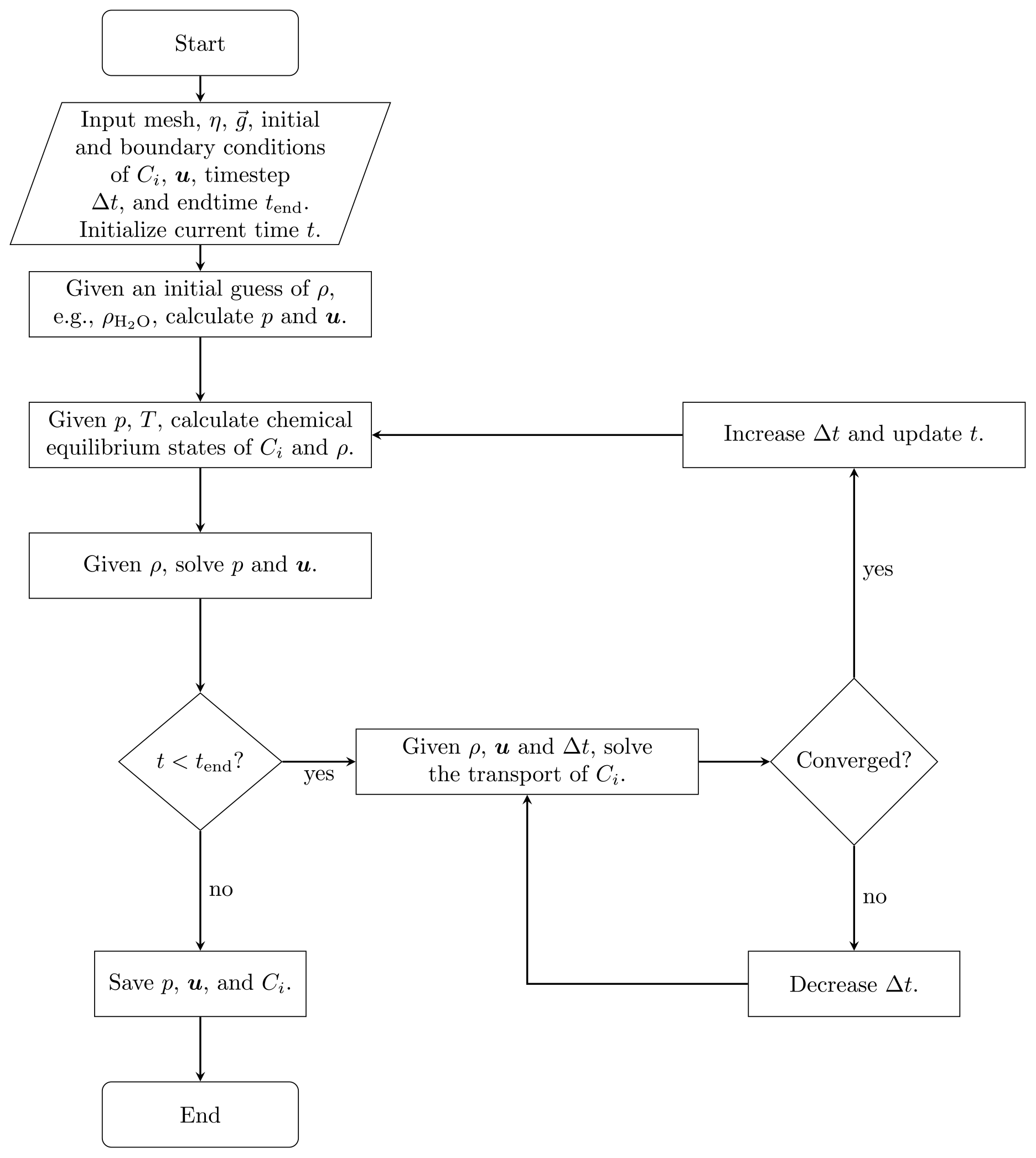
Figure 1 Flowchart of the simulation procedures that couple flow, transport, and chemical equilibrium using the sequential non-iterative approach (SNIA).

2.3 Selected experiments for model evaluation

We select three experiments, performed (by others) in a Hele-Shaw cell, to evaluate the effectiveness of the Nernst–Planck model in reactive transport situations. The diffusivities of the aqueous species are listed in Table 1. The density and dynamic viscosity of the relevant aqueous solutions are listed in Table 2. Our models assume constant dynamic viscosity, set as the average viscosity of the aqueous solutions. All experiments are performed in a lab environment, and we assume a constant temperature of 25 ^∘C and a constant background pressure of 100 kPa. No-flow boundary conditions are prescribed on all sides of the simulation domain. Table 3 specifies the chemical compositions of the aqueous solutions, which defines the initial conditions of the mass transport equations.

Table 1 Diffusivities of aqueous species in 25 ^∘C water at infinite dilution.

The diffusivities of aqueous species other than ${\mathrm{HCO}}_{\mathrm{3}}^{-}$, ${\mathrm{CO}}_{\mathrm{3}}^{\mathrm{2}-}$, and CO₂(aq) are taken from Vanýsek (2021). The diffusivities of ${\mathrm{HCO}}_{\mathrm{3}}^{-}$, ${\mathrm{CO}}_{\mathrm{3}}^{\mathrm{2}-}$, and CO₂(aq) are calculated using Zeebe (2011).

Table 2 Dynamic viscosity and density of aqueous solutions and water at 25 ^∘C.

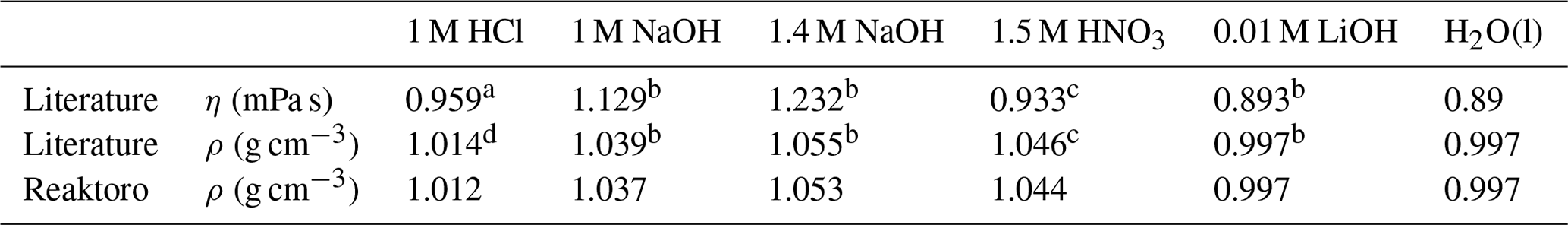
Linearly interpolated using ^a Nishikata et al. (1981), ^b Sipos et al. (2000), ^c Zaytsev and Aseyev (1992), and ^d Åkerlöf and Teare (1938). The viscosity and density of water are taken from Lemmon and Harvey (2021).

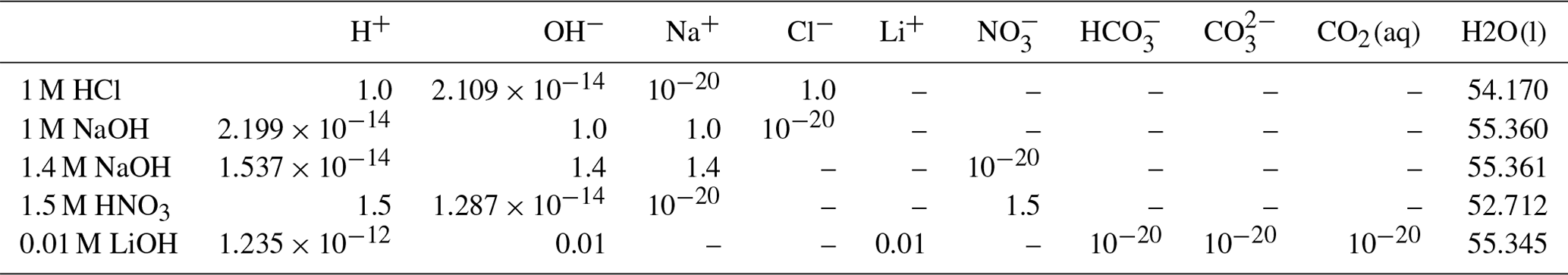
Table 3 The chemical compositions of the aqueous solutions. The chemical compositions are in units of mol L⁻¹. Dashes denote “not applicable” because the chemical species are not considered in the associated simulation cases.

2.3.1 Chemically driven convection of acid–base systems

Almarcha et al. (2010) experimentally showed that simple acid–base reactions, such as $A+B\to C$, can lead to hydrodynamic instabilities due to differences in diffusivities and densities of the chemical species. For the first case in our numerical modeling study, we follow the experimental setup described in Almarcha et al. (2010). The acid (A) is 1 M HCl and the base (B) is 1 M NaOH, where M is the molar concentration (mol L⁻¹). The experiment was performed by Almarcha et al. (2010) in a Hele-Shaw cell, which was 3.1 cm wide, 5 cm high, and had a 0.5 mm gap width. To prevent Rayleigh–Taylor instability, the less dense acid was placed on top of the base. We consider the following species as the main fluid components in this case: H⁺, OH⁻, Na⁺, Cl⁻, and H₂O(l). Please refer to Fig. 2 for the setup. Table 3 lists the chemical composition of 1 M HCl and 1 M NaOH. The prescribed minimum time step size is $\mathrm{3}\times {\mathrm{10}}^{-\mathrm{2}}$ s, and the maximum time step size is 2.0 s.

For the second modeling case, we choose a similar experiment with a strikingly different instability process. In their chemically driven convection experiments, Bratsun et al. (2017) reported a shockwave-like structure of the acid–base interface. In further studies, this phenomenon has subsequently been reproduced using many different acid–base pairs (Mizev et al., 2021; Bratsun et al., 2021). For our numerical comparison study, we use the acid–base pair from Bratsun et al. (2021), i.e., HNO₃–NaOH. The acid consists of 1.5 M HNO₃ and is placed on top of 1.4 M NaOH. The Hele-Shaw cell of this experiment has a width of 2.5 cm, a height of 9.0 cm, and a gap width of 1.2 mm. We consider the following species as the main fluid components in this case: H⁺, OH⁻, Na⁺, ${\mathrm{NO}}_{\mathrm{3}}^{-}$, and H₂O(l). The setup is shown in Fig. 2, and Table 3 lists the initial chemical composition of 1.5 M HNO₃ and 1.4 M NaOH. The prescribed minimum time step size is $\mathrm{1}\times {\mathrm{10}}^{-\mathrm{3}}$ s, and the maximum time step size is 1.0 s. We perform the simulation in a 2D geometry with the same width, height, and species initial conditions as in the experiment and compare the simulation results with the time series of interferometry snapshots taken during the experiments.

2.3.2 Convective dissolution of CO₂ in reactive alkaline solutions

Thomas et al. (2016) performed experiments of convective dissolution of CO₂ in reactive alkaline solutions. The experiment setup consisted of a Hele-Shaw cell saturated with alkaline solutions, where gaseous CO₂ flows over the top of the Hele-Shaw cell. Eventually, gaseous CO₂ dissolves into the alkaline solution, leading to density changes in the solution and, as a result, the formation of convection cells. Furthermore, Thomas et al. (2018) studied the convective dissolution of CO₂ in various molar concentrations of NaCl solutions using the aforementioned experimental setup. Likewise, Mahmoodpour et al. (2019) studied the effect of various salt solutions on the onset of convective instabilities by conducting experiments within porous media. Similar experimental studies in a sandbox have been performed using dense miscible fluids (Neufeld et al., 2010; Agartan et al., 2015; Guo et al., 2021; Wang et al., 2021; Tsinober et al., 2022). Although such experiments do capture the effects of density-driven flow, electromigration effects are not involved. Other experimental studies of convective dissolution of gaseous CO₂ in aqueous solutions have been conducted in pressure–volume–temperature (PVT) cells (Yang and Gu, 2006), Hele-Shaw cells (Kneafsey and Pruess, 2010; Class et al., 2020; Zhang et al., 2020; Jiang et al., 2020; Teng et al., 2021), and 3D granular porous media (Mahmoodpour et al., 2020; Brouzet et al., 2022). Amarasinghe et al. (2020) reviewed CO₂ dissolution experiments and performed experiments of convective dissolution of CO₂ in a Hele-Shaw cell and porous media under supercritical CO₂ conditions.

Numerical studies of CO₂ convective dissolution have been performed considering the reactive transport of a single component (Azin et al., 2013), a single component with mineral reactions (Babaei and Islam, 2018; Shafabakhsh et al., 2021), a single component in two fluid phases with a resolved gas–fluid boundary (Martinez and Hesse, 2016), multiple components with mineral reactions (Zhang et al., 2011), and multiple components in two fluid phases with mineral reactions (Audigane et al., 2007; Soltanian et al., 2019; Sin and Corvisier, 2019). However, the Nernst–Planck model was not invoked in any of these works.

Using lattice Boltzmann methods with consideration of electrostatic forces, Fu et al. (2020, 2021) investigated how ionic species of various salt solutions with varying concentrations affect the onset time and mass transfer rate of CO₂ convective dissolution. So far, these are the only works we found that account for electromigration effects when modeling the convective dissolution of CO₂.

In the third case of our numerical study, we model the experiment of Thomas et al. (2016) and investigate the reactive transport of CO₂ in a Hele-Shaw cell including the electromigration of species using the Nernst–Planck model. Instead of comparing our results to the experiments at the full scale (165 mm by 210 mm) (Thomas et al., 2016), a simulation domain with a width of 100 mm, a height of 40 mm, and a gap width of 0.5 mm is utilized; see the right panel of Fig. 2. The smaller simulation domain was chosen, as the relevant processes remained within this smaller domain. On the top boundary of the simulation domain, we assume that the gaseous CO₂ and the alkaline brine are always in equilibrium. The alkaline brine is 0.01 M LiOH. We consider the following species as the main fluid components in the case of convective dissolution of CO₂: H⁺, OH⁻, Li⁺, CO₂(aq), ${\mathrm{HCO}}_{\mathrm{3}}^{-}$, ${\mathrm{CO}}_{\mathrm{3}}^{\mathrm{2}-}$, and H₂O(l), and the initial conditions are presented in Table 3. The prescribed minimum and maximum time step sizes are $\mathrm{5}\times {\mathrm{10}}^{-\mathrm{3}}$ and 1.5 s, respectively. In the results section, we present the development of the fingers and the movement of the “shock wave” induced by density, reaction, and electromigration effects.

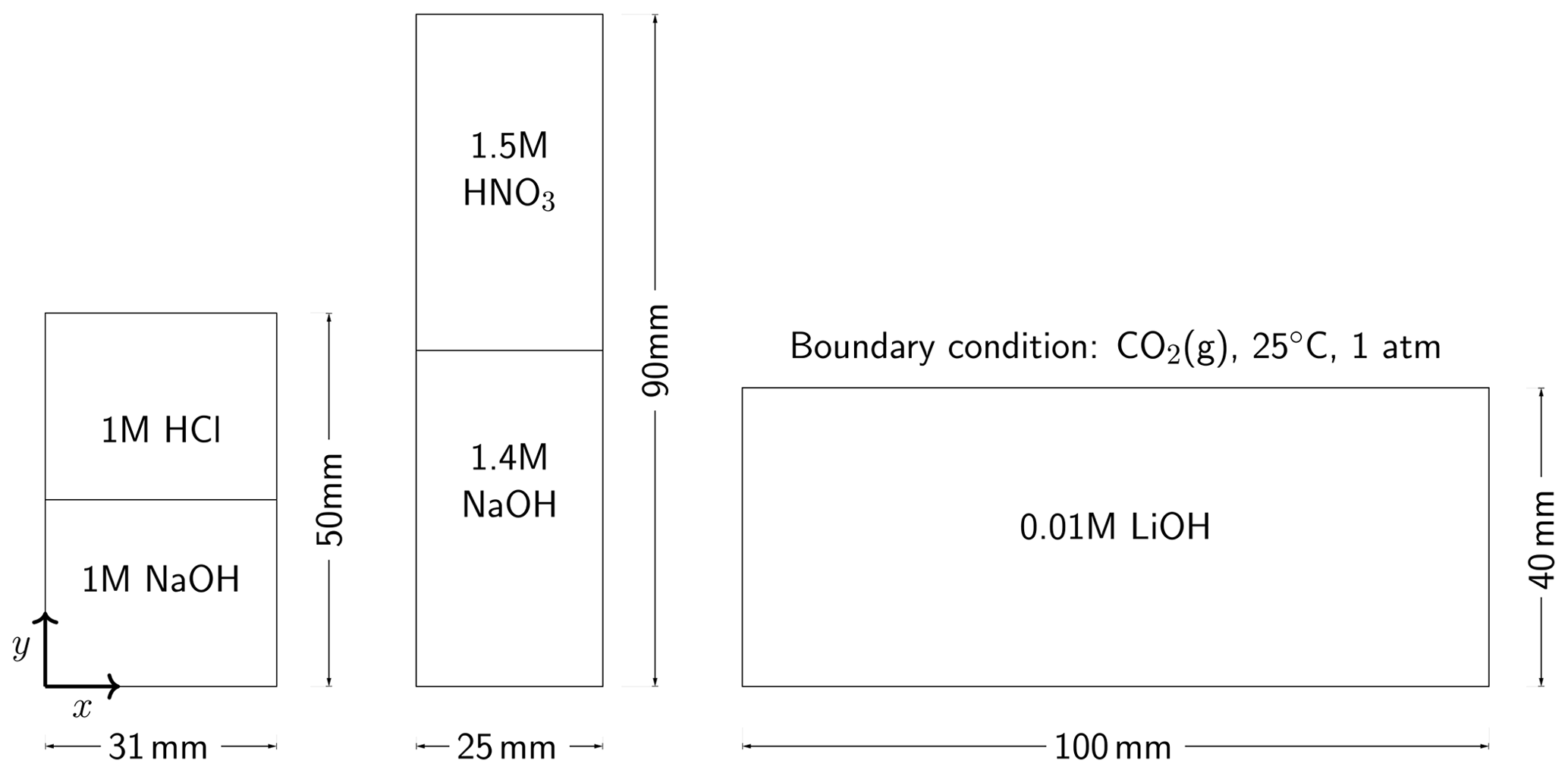
Figure 2 The selected experimental setups. On the left, the chemically driven convection experiments with 1 M HCl–1 M NaOH (Almarcha et al., 2010) are shown. In the middle, the chemically driven convection setup with 1.5 M HNO₃–1.4 M NaOH (Mizev et al., 2021) is shown. On the right, a smaller setup of CO₂ dissolution with 0.01 M LiOH solutions compared to the original setup (165 mm by 210 mm) designed by Thomas et al. (2016) is shown From left to right, the gap widths of the Hele-Shaw cells are 0.5 mm, 1.2 mm, and 0.5 mm, respectively. All Hele-Shaw cells are closed, meaning that no fluid leaves the domain.

3 Results

This section compares the simulations and the experimental results of the chemically driven convection problems and the convective dissolution of CO₂ into a reactive alkaline solution. All simulations are performed using the Nernst–Planck and the single-diffusivity models.

3.1 Comparing the chemically driven convection experiments with the single-diffusivity model and the Nernst–Planck model

We present the results of the chemically driven convection between 1 M HCl and 1 M NaOH solutions. Figure 3 compares the digital interferometry images obtained from experiments with the simulated fluid densities. The interferometry images have a size of 13 mm by 23.075 mm, from which we select a sub-region of the same size as the simulations. This region is indicated by the red box in Fig. 3. Note that the interferometry images show the density contrast of the fluids (induced by changes in refractive index) rather than the density itself. Hence, the simulated density plots cannot be compared with the interferometry images pixel by pixel. Nonetheless, in the left panel of Fig. 3, only the simulations with the Nernst–Planck model replicate the experimentally observed fingering effect with a similar number of fingers. At the simulation time of 60 s, a low-density layer (shown in yellow) emerges in the Nernst–Planck model, an effect which cannot be observed in the single-diffusivity model. At 115 s, the low-density layer develops instabilities, causing density-driven flow. However, the time it takes for fingering to commence is longer in the simulations than in the experiments. This delay can be attributed to the finite representation by the numerical scheme of the diffusion and electromigration fluxes at the initially sharp interface between the acid and the base, which could be improved by adaptive mesh refinement or a higher mesh resolution.

Figure 4 compares the images from the physical experiment with our numerical simulations that utilize the Nernst–Planck model with a lag time of 40 s. We further present the filled contours of the Na⁺ molar concentration and the molar concentration of Na⁺ and Cl⁻ combined. Na⁺ is transported upwards, closely following the low-density fingers. The rightmost plots of Fig. 4 show that the low-density region is caused by lower concentrations of both Na⁺ and Cl⁻. The dark red region indicates lower salinity and corresponds to the low-density yellow and turquoise region. More interestingly, a stable region of higher salinity (shown in blue) forms close to the initial contact line of the acid and the base.

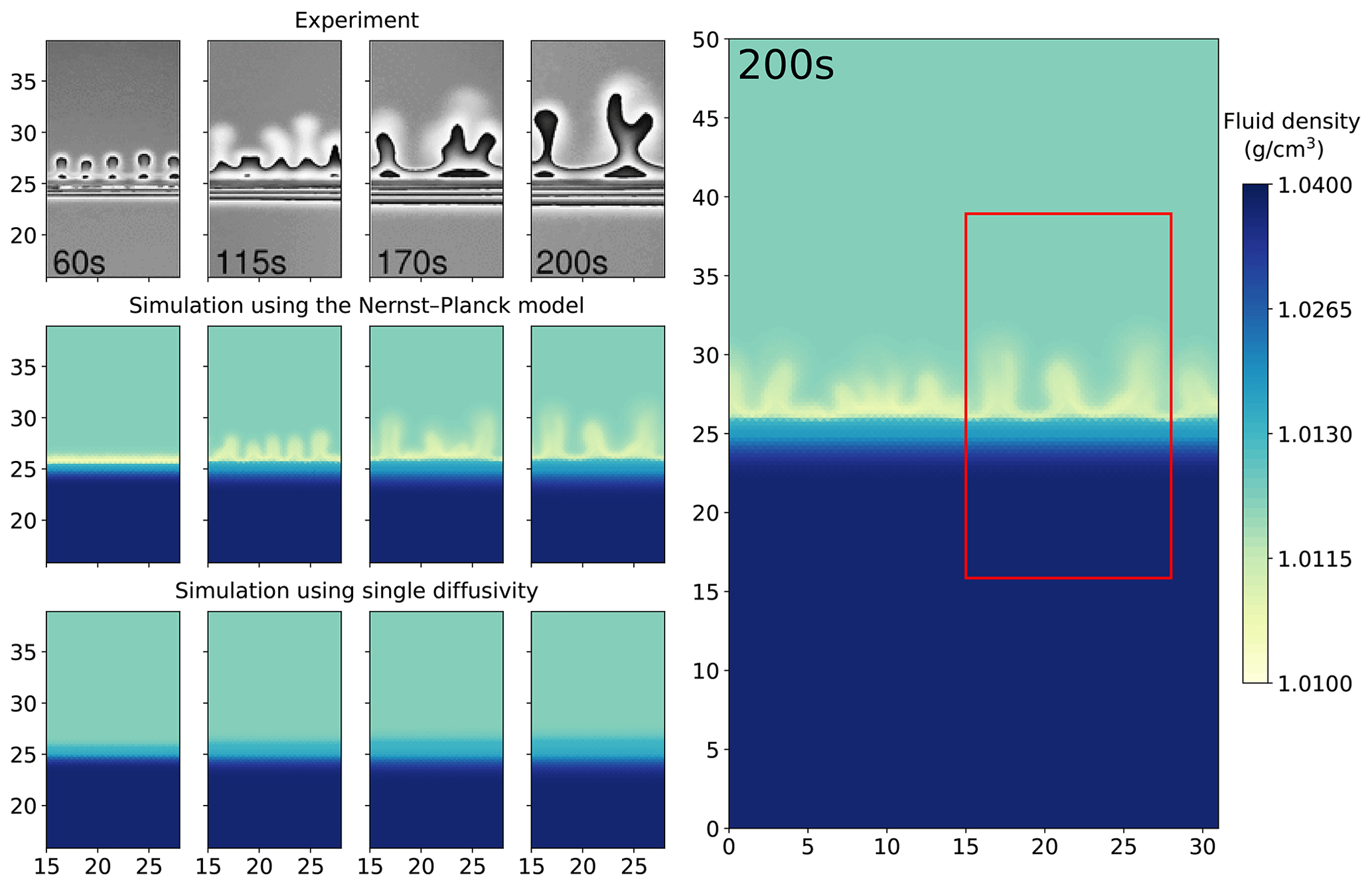
Figure 3 Comparing the simulations using the Nernst–Planck model and those using the single-diffusivity model with the experiments of chemically driven convection in HCl–NaOH solutions. The column on the right shows the full simulation domain (31 mm by 50 mm), and the red box indicates the comparison window. For the four columns on the left, the time increases from left to right, and the simulation time corresponds to the time shown in the experiment snapshots. The experimental figures are based on digital interferometry, and we adapted the figures from Almarcha et al. (2010).

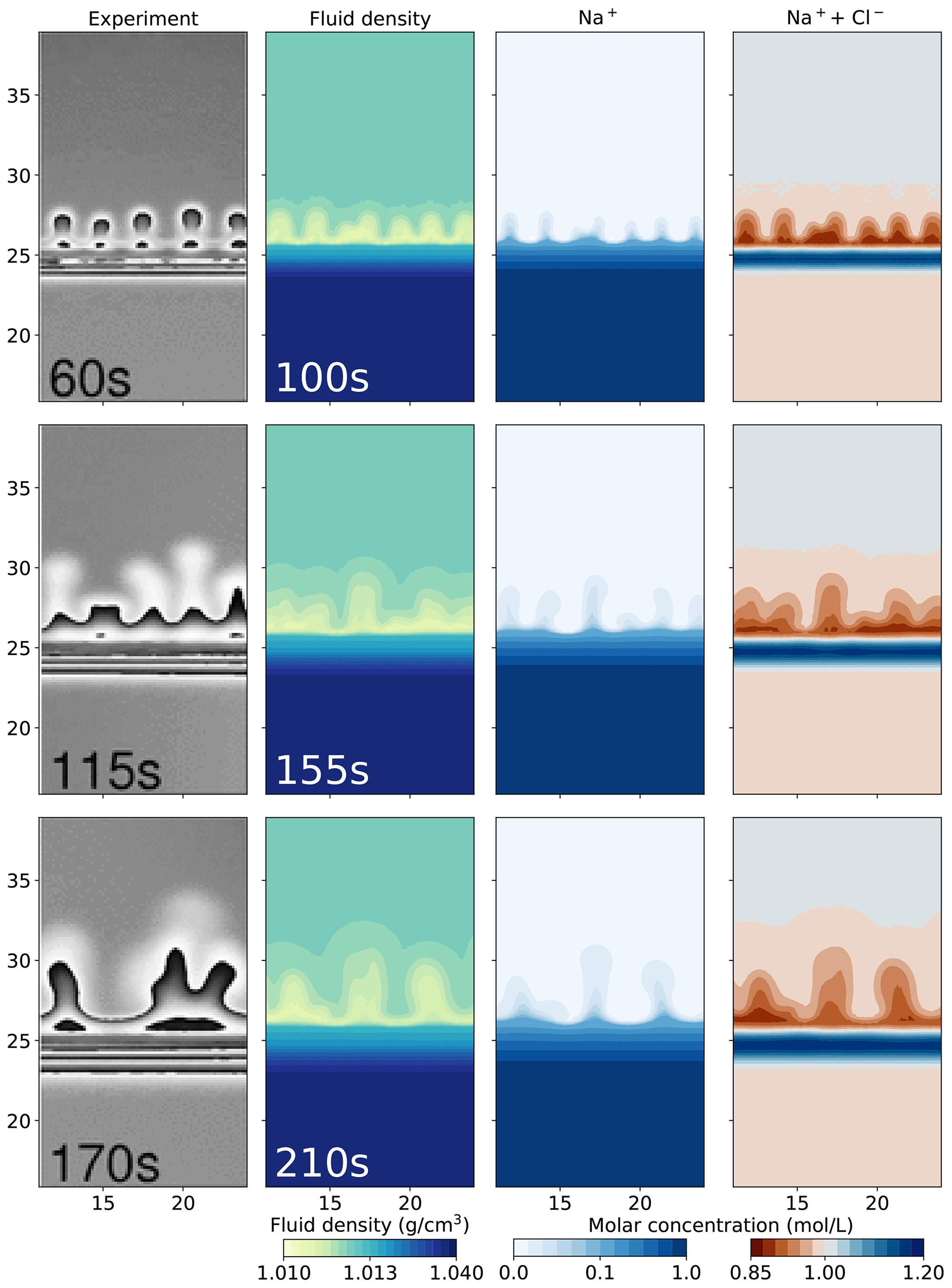
Figure 4 Comparing the simulation results using the Nernst–Planck model with the experimental results of chemically driven convection in HCl–NaOH solutions. The leftmost column shows the experimental figures, adapted from Almarcha et al. (2010). The filled contour plots present the simulation results, showing the fluid density, molar concentration of Na⁺, and the sum of the molar concentrations of Na⁺ and Cl⁻ with a lag time of 40 s.

Figure 5 shows a comparison of the experiments of 1.5 M HNO₃ and 1.4 M NaOH solutions and the simulations. Both the Nernst–Planck model and the single-diffusivity model reproduce the shockwave-like structures seen in the experimental interferometry images, i.e., the rapid downward movement of the acid–base interface. In the interferometry images at the 3 s snapshot, fingers appear, which the simulations cannot reproduce at the 3 s simulation time. As discussed before, during the HCl–NaOH experiments the mismatch is due to the poor approximation of diffusive fluxes at the initially sharp interface. For the later snapshots, 150 and 700 s, we observe the dark lines becoming more sparse in the interferometry images. This indicates that the fluid densities become more homogeneous, and the simulations replicate such mixing physics.

In Fig. 6, we show the simulations of the molar concentrations of Na⁺ and the streamlines of the fluid velocity field at 25, 50, 75, 100, and 125 s. One can clearly see that the Na⁺ plumes follow the streamlines. The maximum velocity in the y direction of the Nernst–Planck simulations and the single-diffusivity simulations during the five presented snapshots are 4.086 and 4.184 mm s⁻¹, respectively. Both models replicate the experiments, and no particular difference can be observed. In such experimental settings, where density-driven convection is dominant, a distinctive description of the diffusive fluxes is less crucial.

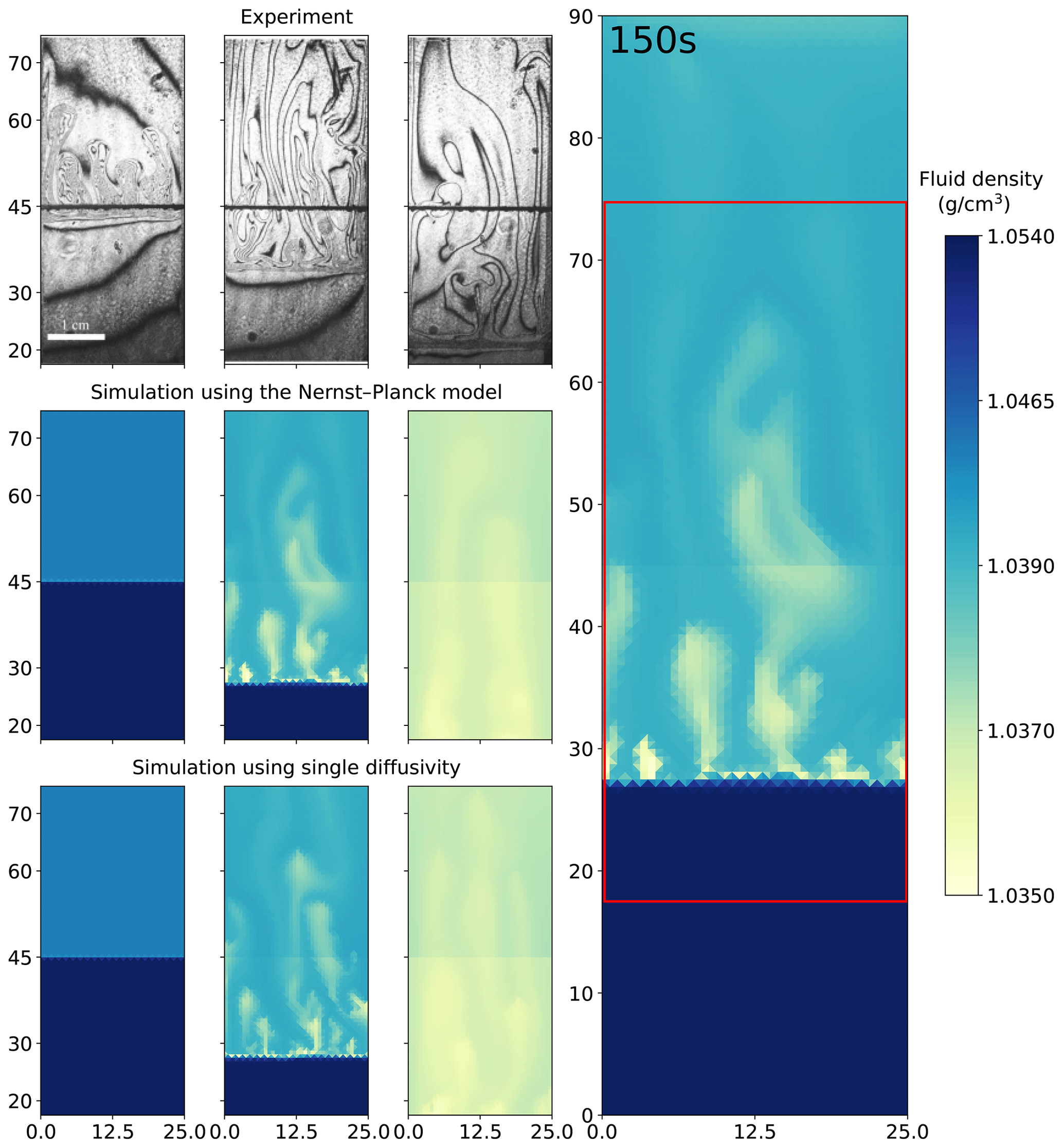
Figure 5 Comparing the simulations using the Nernst–Planck model and those using the single-diffusivity model with the experiments of chemically driven convection in HNO₃–NaOH solutions. The column on the right shows the full simulation domain (25 mm by 90 mm), and the red box indicates the comparison window. In the left columns, the time increases from left to right, where the snapshots correspond to 3, 150, and 700 s. The figures from the experiments are based on digital interferometry, and they were adapted from Mizev et al. (2021).

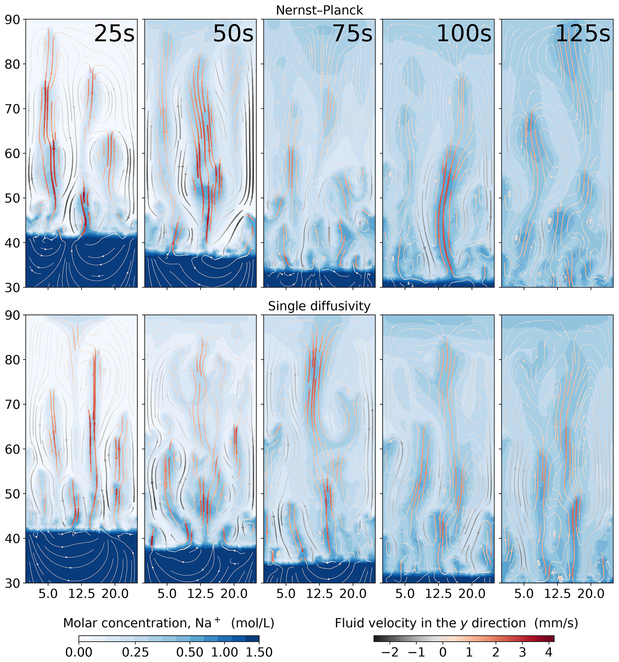
Figure 6 Comparing the simulations using the Nernst–Planck model and those using the single-diffusivity model in modeling chemically driven convection of HNO₃–NaOH solutions. The top and the bottom rows show the simulations employing the Nernst–Planck model and the simulations using one single diffusivity, respectively. The time increases from left to right, and the snapshots correspond to 25, 50, 75, 100, and 125 s.

3.2 Simulation of convective dissolution of CO₂ in reactive alkaline solutions

Figure 7 compares the schlieren images of convective dissolution of CO₂ in 0.01 M LiOH solution from the experiments with the density plots using the Nernst–Planck and the single-diffusivity models. The onset time of the Nernst–Planck model and the single-diffusivity model are approximately 600 and 1400 s, respectively. Therefore, the densities of the two simulation results are shown for the onset time plus the experimental snapshot, 780 s. At these time steps, the convective fingers in both models reach similar depths of ∼17 mm, as shown in the schlieren image from the experiment. The simulation result of the Nernst–Planck model is comparable to the experiment of CO₂ dissolving into the LiOH brine and shows a broader range of finger sizes compared to those of the single-diffusivity model. In contrast, the convective fingers in the single-diffusivity model resemble the fingers seen in the schlieren image, where CO₂ dissolves in H₂O and the electromigration effects are weaker compared to the LiOH solution.

Figure 8 shows the density plots of the simulation results using the Nernst–Planck model and the single-diffusivity model. In the top row, we show the onset of the convective instability. The single-diffusivity model develops instabilities roughly 800 s later than the Nernst–Planck model. The second panel from the top shows the convective fingers after their onset; the Nernst–Planck model yields twice the number of fingers compared to the single-diffusivity model. In these two panels, we observe that the Nernst–Planck model generates a low-density layer, colored in yellow, at the dissolution front, which causes a shorter onset time and more fingers due to a larger density contrast. In the two bottom panels, we show the evolution of the simulations at later times. There are differences in the fingering pattern, such as more secondary convective fingers being generated by the Nernst–Planck model. Moreover, the low-density layer in the Nernst–Planck model persists even at later times.

To further quantify the simulation results, Fig. 9 visualizes the pH plots and the molar concentrations of Li⁺, CO₂(aq), and ${\mathrm{CO}}_{\mathrm{3}}^{\mathrm{2}-}$. We use a diverging color palette to present the acid regions (orange) and the base regions (purple). The molar concentrations of CO₂(aq) and ${\mathrm{CO}}_{\mathrm{3}}^{\mathrm{2}-}$ follow the pH color palette, where most CO₂(aq) exists in the acidic region and most ${\mathrm{CO}}_{\mathrm{3}}^{\mathrm{2}-}$ exists in the basic region. Such changes in the CO₂ states lead to changes in the charge states $z=\mathrm{0},\mathrm{1},\mathrm{2}$ for CO₂(aq), ${\mathrm{HCO}}_{\mathrm{3}}^{-}$, and ${\mathrm{CO}}_{\mathrm{3}}^{\mathrm{2}-}$, respectively. In the Li⁺ plot of the Nernst–Planck simulations, we observe up to 30 % differences in the molar concentration compared to the initial condition (0.01 mol L⁻¹). The red regions are where Li⁺ accumulates, and we can clearly see the interaction between Li⁺ and ${\mathrm{CO}}_{\mathrm{3}}^{\mathrm{2}-}$, whereby Li⁺ migrates towards the double-charged ${\mathrm{CO}}_{\mathrm{3}}^{\mathrm{2}-}$. Meanwhile, the single-diffusivity simulation shows almost no contrast in the filled contours other than due to numerical errors. The difference between the maximum and minimum molar concentrations of Li⁺ is $\sim {\mathrm{10}}^{-\mathrm{8}}$ mol L⁻¹. Using the Nernst–Planck model, we confirm the influence of the inert (spectator) ions in the reactive-transport situation discussed in Thomas et al. (2016).

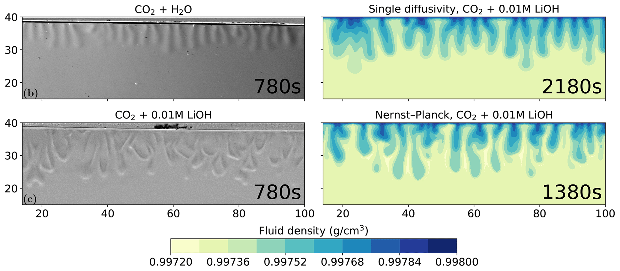
Figure 7 Comparing the simulations using the Nernst–Planck model and those using the single-diffusivity model with the experiments of convective dissolution of CO₂ in 0.01 M LiOH solution. We plot the experimental figure of CO₂ dissolving in pure water in the top-left to demonstrate the differences in fingering patterns compared with CO₂ dissolving in LiOH solution. The filled contours show the fluid density. The experimental figures are adapted from Thomas et al. (2016).

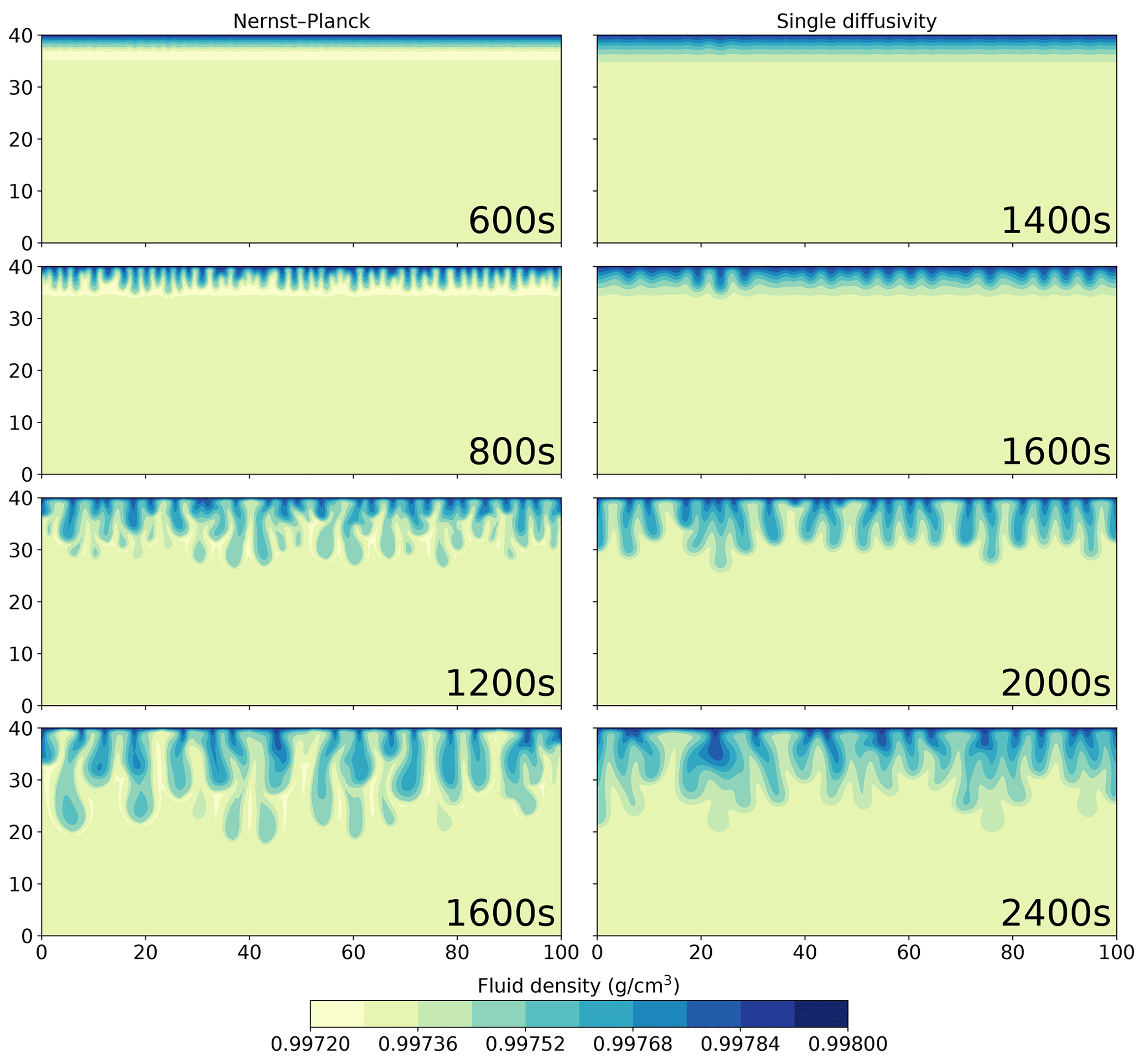
Figure 8 Comparing the simulations using the Nernst–Planck model and those using the single-diffusivity model, while numerically modeling the convective dissolution of CO₂ in 0.01 M LiOH solution. The filled contours show the fluid density. Time increases from top to bottom and is indicated in the plots.

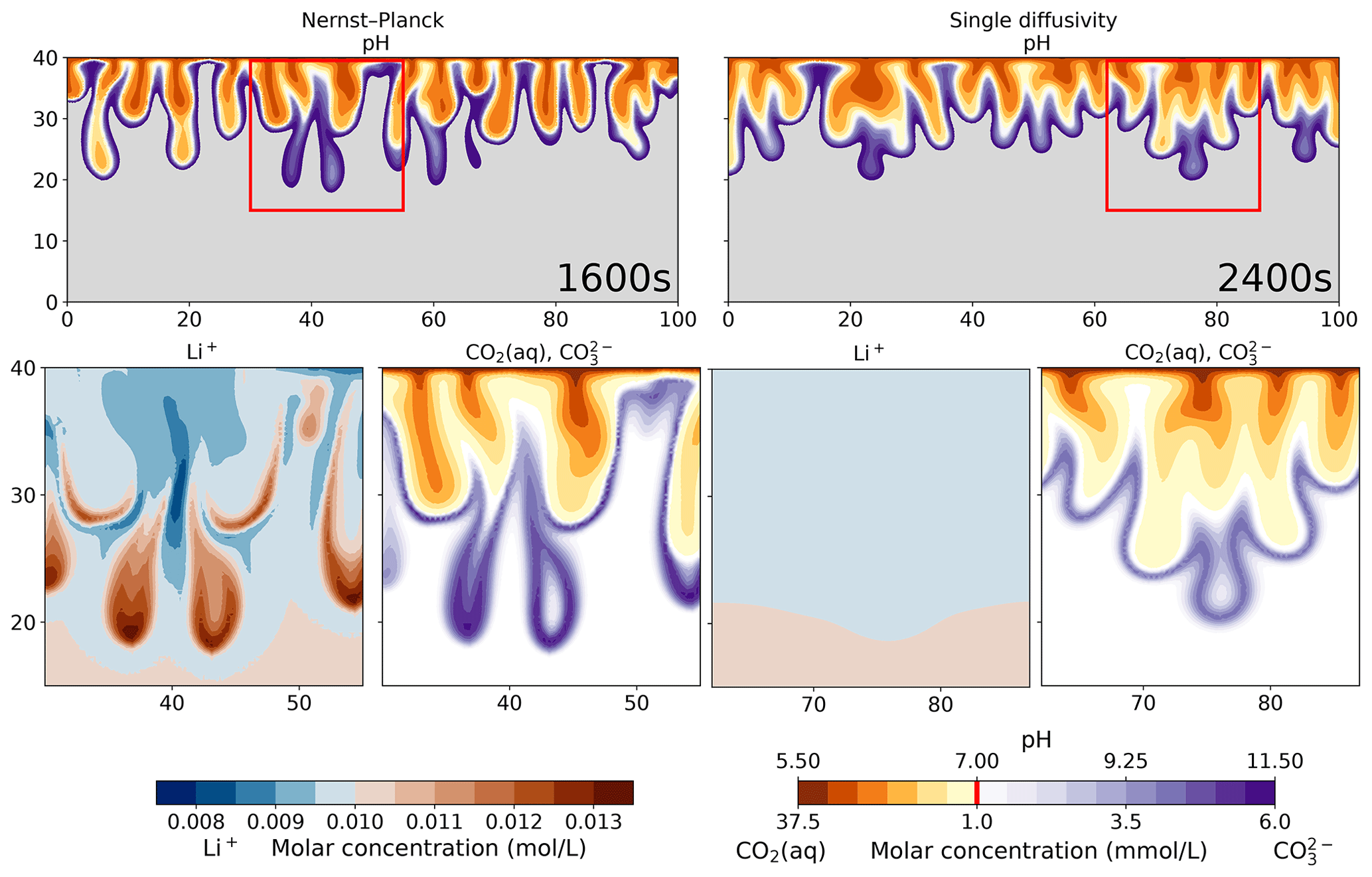
Figure 9 Comparing the simulations using the Nernst–Planck model and those using the single-diffusivity model, while numerically modeling convective dissolution of CO₂ in 0.01 M LiOH solution. The top row shows the pH values. The orange palette represents acidic regions (pH<7), and the purple palette represents basic regions (pH >7). The gray region shows the unperturbed part of the LiOH solution (pH >11.5). In the bottom row, we show the zoomed in view of the red boxes in the top panel. We plot the molar concentrations of Li⁺, CO₂(aq), and ${\mathrm{CO}}_{\mathrm{3}}^{\mathrm{2}-}$. Notice that the molar concentrations of CO₂(aq) and ${\mathrm{CO}}_{\mathrm{3}}^{\mathrm{2}-}$ share the same color bar as the pH values. The vertical red line in the color bar indicates the minimum molar concentrations of CO₂(aq) and ${\mathrm{CO}}_{\mathrm{3}}^{\mathrm{2}-}$ shown in the plots.

4 Discussion

In this section, we discuss whether the Nernst–Planck model is valid, and its differences are compared to the commonly used single-diffusivity model.

4.1 The validity of the Nernst–Planck model under reactive flow conditions

Comparing to two chemically driven convection experiments conducted by Almarcha et al. (2010) and Mizev et al. (2021), we show that the Nernst–Planck numerical model is able to reproduce the convective fingering observed in the experiments, especially in the 1 M HCl–1 M NaOH case. The mechanism that leads to convection is known as the reactive diffusive layer convection (DLC) instability, which arises when a less dense solution of a fast-diffusing component overlies a denser solution of a slow-diffusing component (Lemaigre et al., 2013). In our Nernst–Planck model, the fast-diffusing component is H⁺. Additionally, the convective plumes of the reactive DLC instability are only observed above the initial contact line between the acid and the base (Almarcha et al., 2010; Lemaigre et al., 2013). This is the asymmetric feature of the reactive DLC instability, which can also be observed in the Nernst–Planck simulations (Fig. 3). To directly quote Lemaigre et al. (2013), “the asymmetry of the DLC pattern is related to the chemical reaction which consumes the acid before it can accumulate in the lower layer and replaces it by a third species of intermediate contribution to density”. This third species is salt, a product of the acid–base neutralization reaction. Using the Nernst–Planck model, we not only replicate this stabilizing lower layer but also find that the accumulation of salt can exceed the salt concentration at chemical equilibrium (in this case, approximately 0.5 mol L⁻¹), as shown in Fig. 4.

In the 1.5 M HNO₃–1.4 M NaOH case, both the Nernst–Planck model and the single-diffusivity model reproduce the shockwave-like structure observed in the experiments performed by Mizev et al. (2021). The instability in this case is convection controlled (CC) (Bratsun et al., 2017). The underlying mechanism of this CC instability has previously been attributed to unequal and concentration-dependent diffusivities (Bratsun et al., 2017, 2021, 2022). However, using the single-diffusivity model, our simulations can reproduce the experimental observations. This indicates that modeling CC instabilities is less sensitive to the specific diffusivity model used, as the CC instability is mostly caused by the density-driven convective flow of the reactants. Nevertheless, there are no drawbacks (other than being computationally more intensive) in employing the Nernst–Planck equations to model the CC instability cases.

In the case of CO₂ dissolving in 0.01 M LiOH solution, we observe a much later convective onset time in the numerical simulations than in the experiment by Thomas et al. (2016). This discrepancy is much larger than in the 1 M HCl–1 M NaOH case. It cannot only be explained by the ineffectiveness of the diffusive-flux approximations at the sharp interface of dissolving CO₂(aq). Convective instability can be introduced in a variety of ways in laboratory experiments. For example, interfacial instabilities between the gas and the liquid can occur due to the gas flowing over the interface. Furthermore, if the injected CO₂ is not saturated with water, evaporation of water can induce gravitational instability (Bringedal et al., 2022). These localized physical processes at the gas–liquid boundary, which are not included in our numerical models, could be partly responsible for the later onset times we observe in our simulations.

Although the comparison between the experiment and the simulations of the two models in Fig. 7 can be ambiguous, i.e., the Nernst–Planck model is not the model that describes the schlieren images, we emphasize that the difference between the experiments with Li⁺ and those without it is apparent in the figure. When comparing the Nernst–Planck and the single-diffusivity models, the former exhibits an earlier fingering onset time. This is caused by electromigration effects, which generate the low-density layer shown in Fig. 8. The electromigration of Li⁺, an inert ion in this case, and subsequent effects on the overall transport processes shown in Fig. 9, is clearly a motivation for more studies on the electromigration effects of inert (spectator) ions.

To summarize, we use the experiments conducted by Almarcha et al. (2010), Thomas et al. (2016), Mizev et al. (2021) and our numerical simulation results to show that the Nernst–Planck model is valid in the considered reactive transport scenarios. Particularly in the 1 M HCl–1 M NaOH experiments, where the convective fingers are controlled by diffusion. In the convection-controlled regime, electromigration effects are less crucial, and both the Nernst–Planck model and the single-diffusivity model replicate the 1.5 M HNO₃–1.4 M NaOH experiments well. In the case of CO₂ dissolving in an alkaline solution, the use of the Nernst–Planck model uncovers intricate details of how inert ionic species can affect the overall reactive transport processes.

4.2 Electromigration and the relevance of inert ionic species

Using the simulations of chemically driven convection in 1 M HCl–1 M NaOH solutions, we elaborate the main differences between the Nernst–Planck model and the single-diffusivity model. The top panel of Fig. 10 shows the molar concentrations of salt, plotted against elevation in the Hele-Shaw cell. As expected, the single-diffusivity model shows the concentration profile of two diffusing Heaviside step functions of Na⁺ and Cl⁻. We plot the sum of Na⁺ and Cl⁻ molar concentrations to demonstrate that in single-diffusivity models, Na⁺ and Cl⁻ exhibit an ideal behavior, known as equimolar counter-diffusion. The Nernst–Planck model shows unexpected results, such as the accumulation of Na⁺ and Cl⁻ close to the acid–base boundary. The accumulation can be attributed to a larger diffusivity of the acid components, H⁺ ($\mathrm{9.311}\times {\mathrm{10}}^{-\mathrm{3}}$ mm² s⁻¹) and Cl⁻ ($\mathrm{2.032}\times {\mathrm{10}}^{-\mathrm{3}}$ mm² s⁻¹), compared to the base components, OH⁻ ($\mathrm{5.273}\times {\mathrm{10}}^{-\mathrm{3}}$ mm² s⁻¹) and Na⁺ ($\mathrm{1.334}\times {\mathrm{10}}^{-\mathrm{3}}$ mm² s⁻¹), which leads to more Cl⁻ migrating into the base. One might get the impression that this observation can be modeled by employing multiple diffusivities in the single-diffusivity model. However, we emphasize that the Nernst–Planck model has to be utilized to maintain electroneutrality at the continuum scale. Closely inspecting the fluid density profile, the deficit in salt concentration leads to a lower density than the acid, which causes the reactive DLC instability. The single-diffusivity model is unable to depict the accumulation or deficit in the salt concentrations.

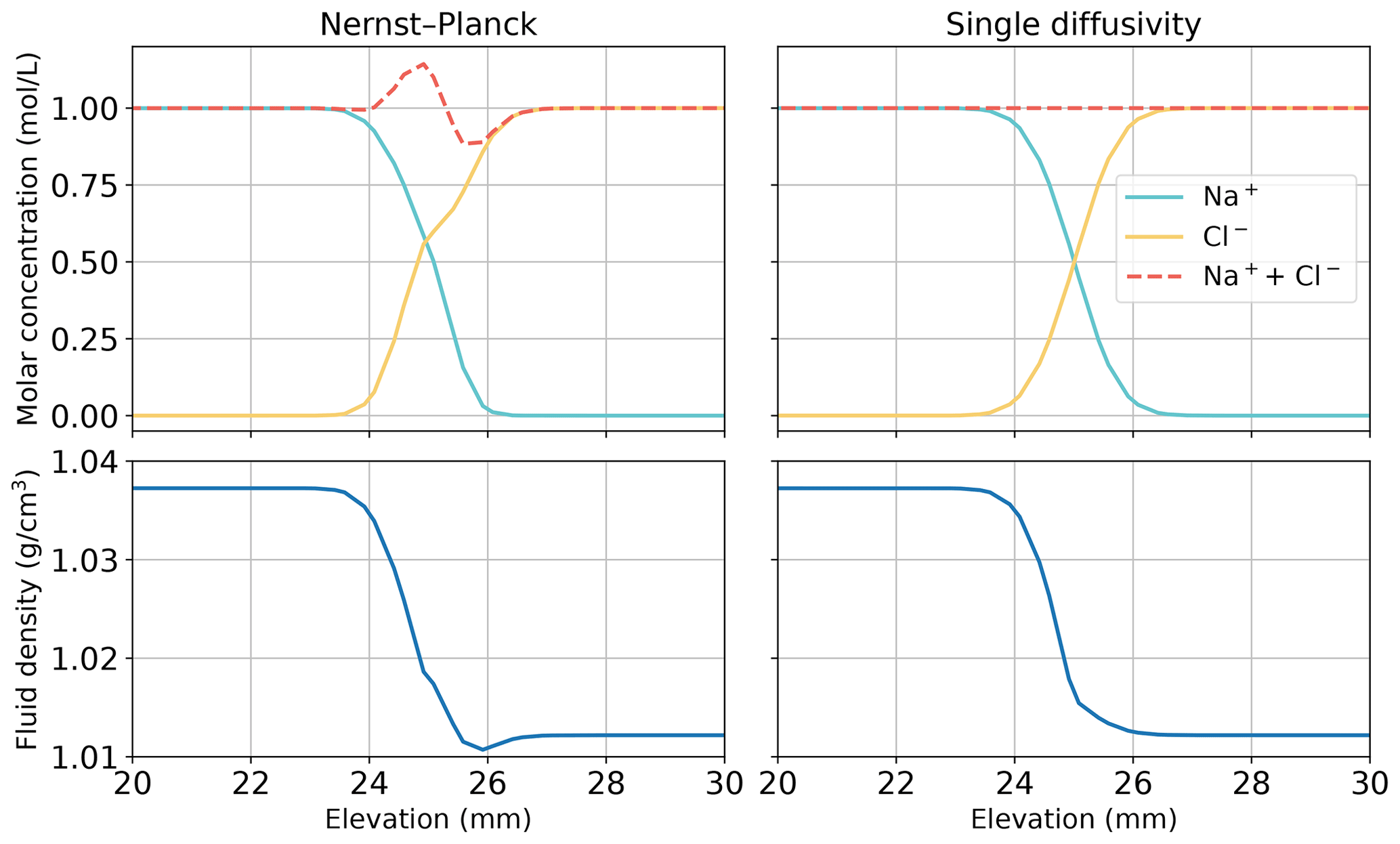
Figure 10 Comparing the simulations using the Nernst–Planck model and those using the single-diffusivity model in modeling chemically driven convection in 1 M HCl–1 M NaOH solutions. The snapshot is given at t=60 s, when fingers have not yet appeared (see Fig. 3). We plot the molar concentrations of salt and the fluid density against elevation in the Hele-Shaw cell, focusing on the contact region between the acid and the base (25 mm).

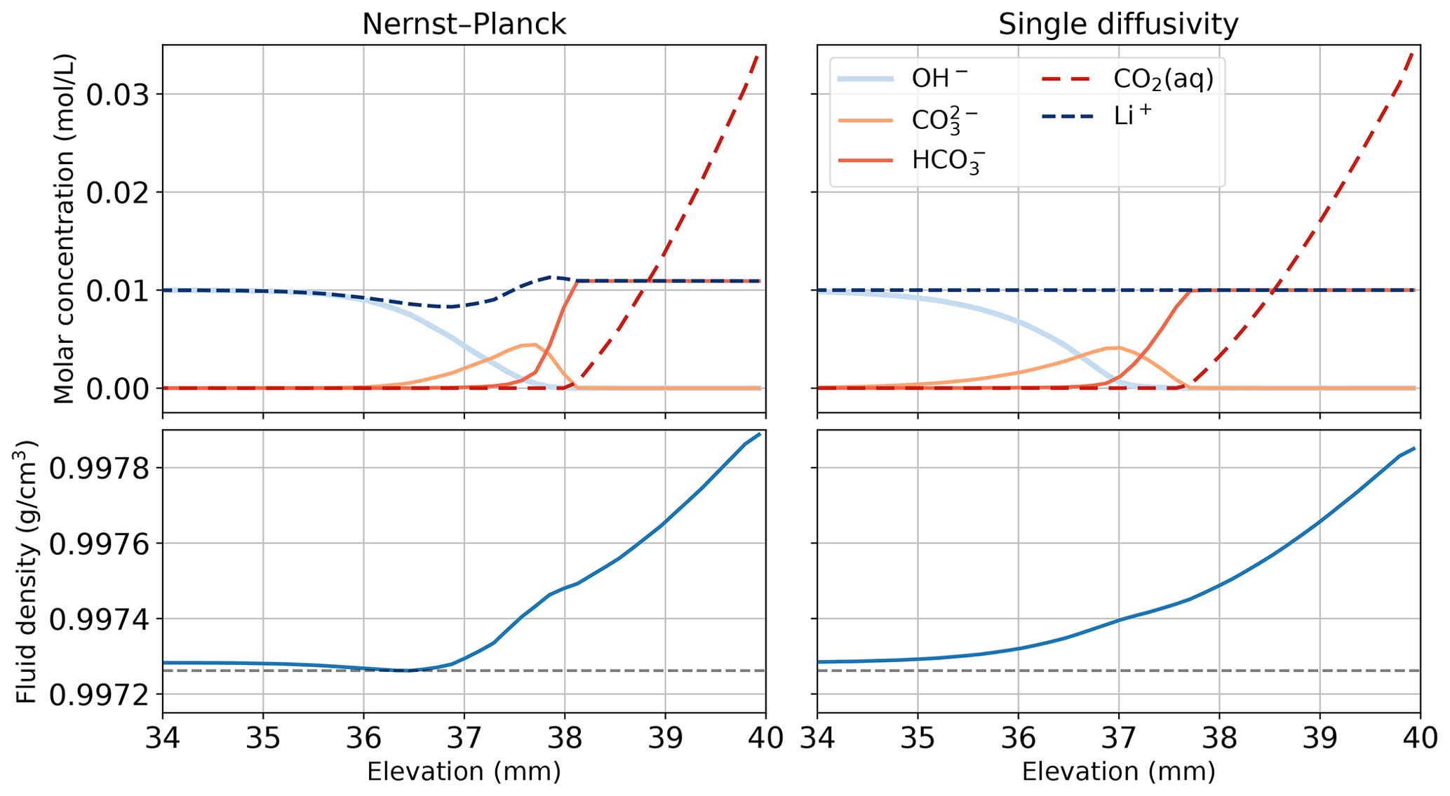
Figure 11 Comparing the simulations using the Nernst–Planck model and those using the single-diffusivity model in modeling convective dissolution of CO₂ in 0.01 M LiOH solution. The snapshot is given at t=600 s, when fingers have not yet appeared (see Fig. 8). We plot the molar concentrations of Li⁺, OH⁻, ${\mathrm{CO}}_{\mathrm{3}}^{\mathrm{2}-}$, ${\mathrm{HCO}}_{\mathrm{3}}^{-}$, and CO₂(aq) and the fluid density against elevation in the Hele-Shaw cell, focusing on the regions close to the top boundary of the Hele-Shaw cell. The horizontal dashed gray lines in the bottom panel show the minimum density observed in the Nernst–Planck model at t=600 s.

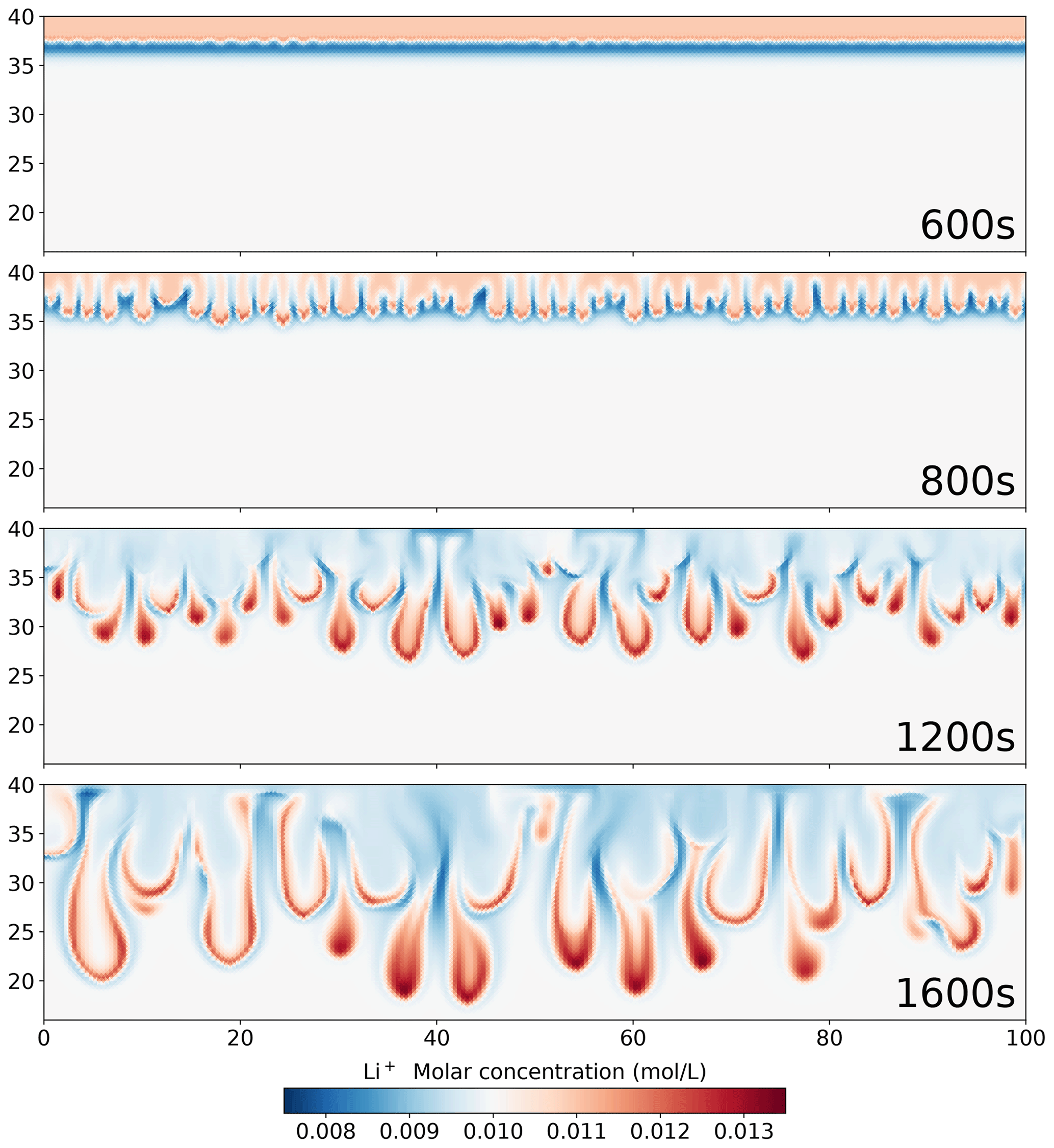
Figure 12 Simulation results using the Nernst–Planck model, showing the molar concentration of Li⁺ during the convective dissolution of CO₂ in 0.01 M LiOH solution.

Moreover, the only reaction that occurs in this experiment is the neutralization reaction

$$\begin{array}{}\text{(39)}& {\mathrm{H}}^{+}+{\mathrm{OH}}^{-}\rightleftharpoons {\mathrm{H}}_{\mathrm{2}}\mathrm{O}\left(\mathrm{l}\right).\end{array}$$

No reaction occurs for Na⁺ and Cl⁻. Hence, they are inert (spectator) species. We elaborate on the transport of H⁺, given by

$$\begin{array}{}\text{(40)}& \begin{array}{rl}{\displaystyle \frac{\partial C_{{\mathrm{H}}^{+}}}{\partial t}}& =-\mathrm{\nabla }\cdot \left(-D_{{\mathrm{H}}^{+}{\mathrm{H}}^{+}}\mathrm{\nabla }{C}_{{\mathrm{H}}^{+}}-D_{{\mathrm{H}}^{+}{\mathrm{OH}}^{-}}\mathrm{\nabla }{C}_{{\mathrm{OH}}^{-}}\right.\\ & \left.-D_{{\mathrm{H}}^{+}{\mathrm{Na}}^{+}}\mathrm{\nabla }{C}_{{\mathrm{Na}}^{+}}-D_{{\mathrm{H}}^{+}{\mathrm{Cl}}^{-}}\mathrm{\nabla }{C}_{{\mathrm{Cl}}^{-}}+\mathit{u}{C}_{{\mathrm{H}}^{+}}\right),\end{array}\end{array}$$

where the generalized-diffusion interpretation of the Nernst–Planck equation is applied in Eq. (23) and D_ij is defined by Eq. (24). In the Nernst–Planck model, the inert species contribute to the transport processes in the form of the cross-coupling diffusivities, $D_{{\mathrm{H}}^{+}{\mathrm{Na}}^{+}}$ and $D_{{\mathrm{H}}^{+}{\mathrm{Cl}}^{-}}$, and the concentration gradients, $\mathrm{\nabla }{C}_{{\mathrm{Na}}^{+}}$ and $\mathrm{\nabla }{C}_{{\mathrm{Cl}}^{-}}$. It has also been shown that the cross-coupling diffusivities (without reactions) can lead to hydrodynamic instabilities (Budroni, 2015). Such tight coupling between ionic species does not exist in the single-diffusivity model. Hence, the Nernst–Planck model is more expressive and capable of modeling the intricacies of reactive transport.

To further demonstrate the electromigration effects of the inert species, Fig. 11 shows the species concentration profile of simulations of CO₂ dissolution in 0.01 M LiOH solution. We plot the 600 s snapshot, which is the onset time of the Nernst–Planck model (see Fig. 8). Figure 11 focuses on the concentration profile close to the top boundary, which is the elevation at 40 mm. When CO₂ dissolves into the LiOH solution, the following chemical reactions occur

$$\begin{array}{}\text{(41)}& {\displaystyle }{\mathrm{CO}}_{\mathrm{2}}\left(\mathrm{aq}\right)+{\mathrm{H}}_{\mathrm{2}}\mathrm{O}\left(\mathrm{l}\right)& {\displaystyle }\rightleftharpoons {\mathrm{H}}_{\mathrm{2}}{\mathrm{CO}}_{\mathrm{3}}\left(\mathrm{aq}\right),\text{(42)}& {\displaystyle }{\mathrm{H}}_{\mathrm{2}}{\mathrm{CO}}_{\mathrm{3}}\left(\mathrm{aq}\right)& {\displaystyle }\rightleftharpoons {\mathrm{H}}^{+}+{\mathrm{HCO}}_{\mathrm{3}}^{-},\text{(43)}& {\displaystyle }{\mathrm{H}}^{+}+{\mathrm{OH}}^{-}& {\displaystyle }\rightleftharpoons {\mathrm{H}}_{\mathrm{2}}\mathrm{O}\left(\mathrm{l}\right),\end{array}$$

where H₂CO₃(aq) is a reaction intermediate that we have not considered in our numerical models. These reactions represent the entire process of CO₂(aq) acidifying aqueous solutions. If we add Eqs. (41)–(43), this yields a simplified reaction,

$$\begin{array}{}\text{(44)}& {\mathrm{CO}}_{\mathrm{2}}\left(\mathrm{aq}\right)+{\mathrm{OH}}^{-}\rightleftharpoons {\mathrm{HCO}}_{\mathrm{3}}^{-}.\end{array}$$

In Fig. 11, at elevations above 38 mm, excessive amounts of CO₂(aq) react with OH⁻, producing ${\mathrm{HCO}}_{\mathrm{3}}^{-}$. However, due to the electroneutrality constraints, the concentration of ${\mathrm{HCO}}_{\mathrm{3}}^{-}$ is limited by the concentrations of the cations, particularly Li⁺. When CO₂(aq) migrates deeper into the more basic regions, i.e., elevations between 36–38 mm, another reaction happens,

$$\begin{array}{}\text{(45)}& {\mathrm{HCO}}_{\mathrm{3}}^{-}\rightleftharpoons {\mathrm{H}}^{+}+{\mathrm{CO}}_{\mathrm{3}}^{\mathrm{2}-}.\end{array}$$

In this basic region, ${\mathrm{HCO}}_{\mathrm{3}}^{-}$ donates H⁺ and forms ${\mathrm{CO}}_{\mathrm{3}}^{\mathrm{2}-}$. We can still observe Li⁺ constraining the amount of ${\mathrm{CO}}_{\mathrm{3}}^{-}$ owing to electroneutrality. Another cation that can contribute to electroneutrality is H⁺. However, in this basic region, the amount of H⁺ is negligible. Although Li⁺ is inert and does not take part in the reactions, Eqs. (41)–(45), it is still relevant in the overall reactive transport process. The transport of Li⁺ in the top left of Fig. 11 is evidence of its involvement in the reactive transport process.

Focusing on the density plots in Fig. 11, not only does the Nernst–Planck model produce lower densities than the single-diffusivity model, the density gradient between 37–38 mm is also higher in the Nernst–Planck model. This can explain the earlier onset time of the Nernst–Planck model compared to the onset time of the single-diffusivity model. We end the discussion with Fig. 12, which presents Li⁺ migrating as CO₂ is dissolving and reacting in the solution. The tight coupling between the equilibrium reactions, electromigration effects, and density-driven flow elicits further investigation (both numerically and experimentally).

5 Conclusions

By comparing the single-diffusivity model and the Nernst–Planck model with reaction-driven flow experiments, we have demonstrated the importance and necessity under certain conditions of modeling the electromigration effects between charged species in aqueous environments using the Nernst–Planck model. Our results of simulating the reaction-driven flow experiments and convective dissolution of CO₂ show that non-reacting species (Na⁺, Cl⁻, Li⁺) influence the overall reactive transport process via electromigration effects, which couple the charged species. Such electromigration effects cannot be modeled using the single-diffusivity model, and further studies on quantifying the valid regimes of the single-diffusivity model are recommended. We make the following conclusions.

• By comparing our numerical modeling results to previously published flow experiments, we have shown that the Nernst–Planck model is valid for modeling reactive transport processes. The processes in the experiments considered here are characterized by an intricate interplay between diffusion, reaction, electromigration, and density-driven convection.

• Compared to the often-used single-diffusivity model, the Nernst–Planck model enables the numerical modeling of the electromigration of ionic species introduced by differing species diffusivities, resulting in more numerous and improved physical insights.

• These reaction-driven flow experiments from literature can be further utilized for benchmarking reactive transport codes.