the Creative Commons Attribution 4.0 License.
the Creative Commons Attribution 4.0 License.
 | 05 Jul 2022
Towards automatic finite-element methods for geodynamics via Firedrake
D. Rhodri Davies
Stephan C. Kramer
Sia Ghelichkhan
Angus Gibson
Firedrake is an automated system for solving partial differential equations using the finite-element method. By applying sophisticated performance optimisations through automatic code-generation techniques, it provides a means of creating accurate, efficient, flexible, easily extensible, scalable, transparent and reproducible research software that is ideally suited to simulating a wide range of problems in geophysical fluid dynamics. Here, we demonstrate the applicability of Firedrake for geodynamical simulation, with a focus on mantle dynamics. The accuracy and efficiency of the approach are confirmed via comparisons against a suite of analytical and benchmark cases of systematically increasing complexity, whilst parallel scalability is demonstrated up to 12 288 compute cores, where the problem size and the number of processing cores are simultaneously increased. In addition, Firedrake's flexibility is highlighted via straightforward application to different physical (e.g. complex non-linear rheologies, compressibility) and geometrical (2-D and 3-D Cartesian and spherical domains) scenarios. Finally, a representative simulation of global mantle convection is examined, which incorporates 230 Myr of plate motion history as a kinematic surface boundary condition, confirming Firedrake's suitability for addressing research problems at the frontiers of global mantle dynamics research.
- Article
(14328 KB) - Full-text XML
- BibTeX
- EndNote


Since the advent of plate tectonic theory, there has been a long and successful history of research software development within the geodynamics community. The earliest modelling tools provided fundamental new insight into the process of mantle convection, its sensitivity to variations in viscosity, and its role in controlling Earth's surface plate motions and heat transport (e.g. McKenzie, 1969; Minear and Toksoz, 1970; Torrance and Turcotte, 1971; McKenzie et al., 1973). Although transformative at the time, computational and algorithmic limitations dictated that these tools were restricted to a simplified approximation of the underlying physics and, excluding some notable exceptions (e.g. Baumgardner, 1985; Glatzmaier, 1988), to 2-D Cartesian geometries. They were specifically designed to address targeted scientific questions. As such, they offered limited flexibility, were not easily extensible, and were not portable across different platforms. Furthermore, since they were often developed for use by one or two expert practitioners, they were poorly documented: details of the implementation could only be determined by analysing the underlying code, which was often a non-trivial and specialised task.
Growing computational resources and significant theoretical and algorithmic advances have since underpinned the development of more advanced research software, which incorporates, for example, better approximations to the fundamental physical principles, including compressibility (e.g. Jarvis and McKenzie, 1980; Bercovici et al., 1992; Tackley, 1996; Bunge et al., 1997; Gassmoller et al., 2020), mineralogical-phase transformations (e.g. Tackley et al., 1993; Nakagawa et al., 2009; Hunt et al., 2012), multi-phase flow (e.g. Katz and Weatherley, 2012; Wilson et al., 2014), variable and non-linear rheologies (e.g. Moresi and Solomatov, 1995; Bunge et al., 1996; Trompert and Hansen, 1998; Tackley, 2000; Moresi et al., 2002; Jadamec and Billen, 2010; Stadler et al., 2010; Alisic et al., 2010; Le Voci et al., 2014; Garel et al., 2014; Jadamec, 2016), and feedbacks between chemical heterogeneity and buoyancy (e.g. van Keken, 1997; Tackley and Xie, 2002; Davies et al., 2012). In addition, these more recent tools can often be applied in more representative 2-D cylindrical and/or 3-D spherical shell geometries (e.g. Baumgardner, 1985; Bercovici et al., 1989; Jarvis, 1993; Bunge et al., 1997; van Keken and Ballentine, 1998; Zhong et al., 2000, 2008; Tackley, 2008; Wolstencroft et al., 2009; Stadler et al., 2010; Davies et al., 2013). The user base of these tools has rapidly increased, with software development teams emerging to enhance their applicability and ensure their ongoing functionality. These teams have done so by adopting best practices in modern software development, including version control, unit and regression testing across a range of platforms and validation of model predictions against a suite of analytical and benchmark solutions (e.g. Blankenbach et al., 1989; Busse et al., 1994; King et al., 2010; Tosi et al., 2015; Kramer et al., 2021a).
Nonetheless, given rapid and ongoing improvements in algorithmic design and software engineering alongside the development of robust and flexible scientific computing libraries that provide access to much of the low-level numerical functionality required by geodynamical models, a next generation of open-source and community-driven geodynamical research software has emerged, exploiting developments from the forefront of computational engineering. This includes ASPECT (e.g. Kronbichler et al., 2012; Heister et al., 2017; Bangerth et al., 2020), built on the deal.II (Bangerth et al., 2007), p4est (Burstedde et al., 2011) and Trilinos (Heroux et al., 2005) libraries, Fluidity (e.g. Davies et al., 2011; Kramer et al., 2012, 2021a, b), which is underpinned by the PETSc (Balay et al., 1997, 2021a, b) and Spud (Ham et al., 2009) libraries, Underworld2 (e.g. Moresi et al., 2007; Beucher et al., 2019), core aspects of which are built on the St Germain (Quenette et al., 2007) and PETSc libraries, and TerraFERMA (Wilson et al., 2017), which has foundations in the FEniCS (Logg et al., 2012; Alnes et al., 2014), PETSc and Spud libraries. By building on existing computational libraries that are highly efficient, extensively tested and validated, modern geodynamical research software is becoming increasingly reliable and reproducible. Its modular design also facilitates the addition of new features and provides a degree of confidence about the validity of previous developments, as evidenced by growth in the use and applicability of ASPECT over recent years.
However, even with these modern research software frameworks, some fundamental development decisions, such as the core physical equations, numerical approximations and general solution strategy, have been integrated into the basic building blocks of the code. Whilst there remains some flexibility within the context of a single problem, modifications to include different physical approximations or components, which can affect non-linear coupling and associated solution strategies, often require extensive and time-consuming development and testing, using either separate code forks or increasingly complex option systems. This makes reproducibility of a given simulation difficult, resulting in a lack of transparency – even with detailed documentation, specific details of the implementation are sometimes only available by reading the code itself, which, as noted previously, is non-trivial, particularly across different forks or with increasing code complexity (Wilson et al., 2017). This makes scientific studies into the influence of different physical or geometrical scenarios, using a consistent code base, extremely challenging. Those software frameworks that try to maintain some degree of flexibility often do so at the expense of performance: the flexibility to configure different equations, numerical discretisations and solver strategies, in different dimensions and geometries, requires implementation compromises in the choice of optimal algorithms and specific low-level optimisations for all possible configurations.
A challenge that remains central to research software development in geodynamics, therefore, is the need to provide accurate, efficient, flexible, easily extensible, scalable, transparent and reproducible research software that can be applied to simulating a wide range of scenarios, including problems in different geometries and those incorporating different approximations of the underlying physics (e.g. Wilson et al., 2017). However, this requires a large time commitment and knowledge that spans several academic disciplines. Arriving at a physical description of a complex system, such as global mantle convection, demands expertise in geology, geophysics, geochemistry, fluid mechanics and rheology. Discretising the governing partial differential equations (PDEs) to produce a suitable numerical scheme requires proficiency in mathematical analysis, whilst its translation into efficient code for massively parallel systems demands advanced knowledge in low-level code optimisation and computer architectures (e.g. Rathgeber et al., 2016). The consequence of this is that the development of research software for geodynamics has now become a multi-disciplinary effort, and its design must enable scientists across several disciplines to collaborate effectively, without requiring each of them to comprehend all aspects of the system.
Key to achieving this is to abstract, automate and compose the various processes involved in numerically solving the PDEs governing a specific problem (e.g. Logg et al., 2012; Alnes et al., 2014; Rathgeber et al., 2016; Wilson et al., 2017) to enable a separation of concerns between developing a technique and using it. As such, software projects involving automatic code generation have become increasingly popular, as these help to separate different aspects of development. Such an approach facilitates collaboration between computational engineers with expertise in hardware and software, computer scientists and applied mathematicians with expertise in numerical algorithms, and domain-specific scientists, such as geodynamicists.
In this study, we introduce Firedrake to the geodynamical modelling community: a next-generation automated system for solving PDEs using the finite-element method (e.g. Rathgeber et al., 2016; Gibson et al., 2019). As we will show, the finite-element method is well-suited to automatic code-generation techniques: a weak formulation of the governing PDEs, together with a mesh, initial and boundary conditions, and appropriate discrete function spaces, is sufficient to fully represent the problem. The purpose of this paper is to demonstrate the applicability of Firedrake for geodynamical simulation whilst also highlighting its advantages over existing geodynamical research software. We do so via comparisons against a suite of analytical and benchmark cases of systematically increasing complexity.
The remainder of the paper is structured as follows. In Sect. 2, we provide a background to the Firedrake project and the various dependencies of its software stack. In Sect. 3, we introduce the equations governing mantle convection which will be central to the examples developed herein, followed, in Sect. 4, by a description of their discretisation via the finite-element method and the associated solution strategies. In Sect. 5, we introduce a series of benchmark cases in Cartesian and spherical shell geometries. These are commonly examined within the geodynamical modelling community, and we describe the steps involved with setting up these cases in Firedrake, allowing us to highlight its ease of use. Parallel performance is analysed in Sect. 6, with a representative example of global mantle convection described and analysed in Sect. 7. The latter case confirms Firedrake's suitability for addressing research problems at the frontiers of global mantle dynamics research. Other components of Firedrake, which have not been showcased in this paper but which may be beneficial to various future research endeavours, are discussed in Sect. 8.
The Firedrake project is an automated system for solving partial differential equations using the finite-element method (e.g. Rathgeber et al., 2016). Using a high-level language that reflects the mathematical description of the governing equations (e.g. Alnes et al., 2014), the user specifies the finite-element problem symbolically. The high-performance implementation of assembly operations for the discrete operators is then generated “automatically” by a sequence of specialised compiler passes that apply symbolic mathematical transformations to the input equations to ultimately produce C (and C++) code (Rathgeber et al., 2016; Homolya et al., 2018). Firedrake compiles and executes this code to create linear or non-linear systems, which are solved by PETSc (Balay et al., 1997, 2021b, a). As stated by Rathgeber et al. (2016), in comparison to conventional finite-element libraries, and even more so with handwritten code, Firedrake provides a higher-productivity mechanism for solving finite-element problems whilst simultaneously applying sophisticated performance optimisations that few users would have the resources to code by hand.
Firedrake builds on the concepts and some of the code of the FEniCS project (e.g. Logg et al., 2012), particularly its representation of variational problems via the Unified Form Language (UFL) (Alnes et al., 2014). We note that the applicability of FEniCS for geodynamical problems has already been demonstrated (e.g. Vynnytska et al., 2013; Wilson et al., 2017). Both frameworks have the goal of saving users from manually writing low-level code for assembling the systems of equations that discretise their model physics. An important architectural difference is that, while FEniCS has components written in C++ and Python, Firedrake is completely written in Python, including its run-time environment (it is only the automatically generated assembly code that is in C/C++, although it does leverage the PETSc library, written in C, to solve the assembled systems, albeit through its Python interface – petsc4py). This provides a highly flexible user interface with ease of introspection of data structures. We note that the Python environment also allows deployment of handwritten C kernels should the need arise to perform discrete mesh-based operations that cannot be expressed in the finite-element framework, such as sophisticated slope limiters or bespoke sub-grid physics.
Firedrake offers several highly desirable features, rendering it well-suited to problems in geophysical fluid dynamics. As will be illustrated through a series of examples below, of particular importance in the context of this paper is Firedrake's support for a range of different finite-element discretisations, including a highly efficient implementation of those based on extruded meshes, programmable non-linear solvers and composable operator-aware solver preconditioners. As the importance of reproducibility in the computational geosciences is increasingly recognised, we note that Firedrake integrates with Zenodo and GitHub to provide users with the ability to generate a set of DOIs corresponding to the exact set of Firedrake components used to conduct a particular simulation, in full compliance with FAIR (findable, accessible, interoperable, reusable) principles.
2.1 Dependencies
Firedrake treats finite-element problems as a composition of several abstract processes, using separate packages for each. The framework imposes a clear separation of concerns between the definition of the problem (UFL, Firedrake language), the generation of computational kernels used to assemble the coefficients of the discrete equations (Two-Stage Form Compiler – TSFC – and FInAT), the parallel execution of this kernel (PyOP2) over a given mesh topology (DMPlex) and the solution of the resulting linear or non-linear systems (PETSc). These layers allow various types of optimisation to be applied at different stages of the solution process. The key components of this software stack are described next.
-
UFL – as we will see in the examples below, a core part of finite-element problems is the specification of the weak form of the governing PDEs. UFL, a domain-specific symbolic language with well-defined and mathematically consistent semantics that is embedded in Python, provides an elegant solution to this problem. It was pioneered by the FEniCS project (Logg et al., 2012), although Firedrake has added several extensions.
-
Firedrake language – in addition to the weak form of the PDEs, finite-element problems require the user to select appropriate finite elements, specify the mesh to be employed, set field values for initial and boundary conditions and specify the sequence in which solves occur. Firedrake implements its own language for these tasks, which was designed to be to a large extent compatible with DOLFIN (Logg et al., 2012), the runtime application programming interface (API) of the FEniCS project. We note that Firedrake implements various extensions to DOLFIN, whilst some features of DOLFIN are not supported by Firedrake.
-
FInAT (Kirby and Mitchell, 2019) incorporates all information required to evaluate the basis functions of the different finite-element families supported by Firedrake. In earlier versions of Firedrake this was done through tabulation of the basis functions evaluated at Gauss points (FIAT: Kirby, 2004). FInAT, however, provides this information to the form compiler as a combination of symbolic expressions and numerical values, allowing for further optimisations. FInAT allows Firedrake to support a wide range of finite elements, including continuous, discontinuous, H(div) and H(curl) discretisations and elements with continuous derivatives such as the Argyris and Bell elements.
-
TSFC – a form compiler takes a high-level description of the weak form of PDEs (here in the UFL) and produces low-level code that carries out the finite-element assembly. Firedrake uses the TSFC, which was developed specifically for the Firedrake project (Homolya et al., 2018), to generate its local assembly kernels. TSFC invokes two stages, where in the first stage UFL is translated to an intermediate symbolic tensor algebra language before translating this into assembly kernels written in C. In comparison to the form compilers of FEniCS (FFC and UFLACS), TSFC aims to maintain the algebraic structure of the input expression for longer, which opens up additional opportunities for optimisation.
-
PyOP2 – a key component of Firedrake's software stack is PyOP2, a high-level framework that optimises the parallel execution of computational kernels on unstructured meshes (Rathgeber et al., 2012; Markall et al., 2013). Where the local assembly kernels generated by TSFC calculate the values of a local tensor from local input tensors, all associated with the degrees of freedom (DOFs) of a single element, PyOP2 wraps this code in an additional layer responsible for the extraction and addition of these local tensors out of/into global structures such as vectors and sparse matrices. It is also responsible for the maintenance of halo layers, the overlapping regions in a parallel decomposed problem. PyOP2 allows for a clean separation of concerns between the specification of the local kernel functions, in which the numerics of the method are encoded, and their efficient parallel execution. More generally, this separation of concerns is the key novel abstraction that underlies the design of the Firedrake system.
-
DMPlex – PyOP2 has no concept of the topological construction of a mesh. Firedrake derives the required maps through DMPlex, a data management abstraction that represents unstructured mesh data, which is part of the PETSc project (Knepley and Karpeev, 2009). This allows Firedrake to leverage the DMPlex partitioning and data migration interfaces to perform domain decomposition at run time whilst supporting multiple mesh file formats. Moreover, Firedrake reorders mesh entities to ensure computational efficiency (Lange et al., 2016).
-
Linear and non-linear solvers – Firedrake passes solver problems on to PETSc (Balay et al., 1997, 2021a, b), a well-established, high-performance solver library that provides access to several of its own and third-party implementations of solver algorithms. The Python interface to PETSc (Dalcin et al., 2011) makes integration with Firedrake straightforward. We note that employing PETSc for both its solver library and for DMPlex has the additional advantage that the set of library dependencies required by Firedrake is kept small (Rathgeber et al., 2016).
Our focus here is on mantle convection, the slow creeping motion of Earth's mantle over geological timescales. The equations governing mantle convection are derived from the conservation laws of mass, momentum and energy. The simplest mathematical formulation assumes a single incompressible material and the Boussinesq approximation (McKenzie et al., 1973), under which the non-dimensional momentum and continuity equations are given by
where is the stress tensor, u is the velocity and T is the temperature. is the unit vector in the direction opposite to gravity and Ra0 denotes the Rayleigh number, a dimensionless number that quantifies the vigour of convection:
Here, ρ0 denotes the reference density, α the thermal expansion coefficient, ΔT the characteristic temperature change across the domain, g the gravitational acceleration, d the characteristic length, μ0 the reference dynamic viscosity and κ the thermal diffusivity. Note that the above non-dimensional equations are obtained through the following characteristic scales: length d, time and temperature ΔT.
When simulating incompressible flow, the full stress tensor, , is decomposed into deviatoric and volumetric components:
where is the deviatoric stress tensor, p is dynamic pressure and I is the identity matrix. Substituting Eq. (4) into Eq. (1) and utilizing the constitutive relation
which relates the deviatoric stress tensor, , to the strain-rate tensor, , yields
The viscous flow problem can thus be posed in terms of pressure, p, velocity, u, and temperature, T. The evolution of the thermal field is controlled by an advection–diffusion equation:
These governing equations are sufficient to solve for the three unknowns together with adequate boundary and initial conditions.
For the derivation of the finite-element discretisation of Eqs. (6), (2) and (7), we start by writing these in their weak form. We select appropriate function spaces V, W and Q that contain respectively the solution fields for velocity u, pressure p and temperature T and also contain the test functions v,w and q. The weak form is then obtained by multiplying these equations by the test functions and integrating over the domain Ω:
Note that we have integrated by parts the viscosity and pressure gradient terms in Eq. (6) and the diffusion term in Eq. (7) but have omitted the corresponding boundary terms, which will be considered in the following section.
Equations (8)–(10) are a more general representation of the continuous PDEs in strong form (Eqs. 6, 2 and 7), provided suitable function spaces with sufficient regularity are chosen (see for example Zienkiewicz et al., 2005; Elman et al., 2005). Finite-element discretisation proceeds by restricting these function spaces to finite-dimensional subspaces. These are typically constructed by dividing the domain into cells or elements and restricting it to piecewise polynomial subspaces with various continuity requirements between cells. Firedrake offers a very wide range of such finite-element function spaces (see Kirby and Mitchell, 2019, for an overview). It should be noted however that, in practice, this choice is guided by numerical stability considerations in relation to the specific equations that are being solved. In particular, the choice of velocity and pressure function spaces used in the Stokes system is restricted by the Ladyzhenskaya–Babuška–Brezzi (LBB) condition (see Thieulot and Bangerth, 2022, for an overview of common choices for geodynamical flow). In this paper, we focus on the use of the familiar Q2Q1 element pair for velocity and pressure, which employs piecewise continuous bi-quadratic and bilinear polynomials on quadrilaterals or hexahedra for velocity and pressure respectively. In addition, to showcase Firedrake's flexibility, we use the less familiar Q2P1DG pair in a number of cases, in which pressure is discontinuous and piecewise linear (but not bilinear). For temperature, we primarily use a Q2 discretisation but also show some results using a Q1 discretisation.
All that is required for the implementation of these choices is that a basis can be found for the function space such that each solution can be written as a linear combination of basis functions. For example, if we have a basis ϕi of the finite-dimensional function space Qh of temperature solutions, then we can write each temperature solution as
where Ti represents the coefficients that we can collect into a discrete solution vector . Using a Lagrangian polynomial basis, the coefficients Ti correspond to values at the nodes, where each node i is associated with one basis function ϕi, but this is not generally true for other choices of finite-element bases.
In curved domains, boundaries can be approximated with a finite number of triangles, tetrahedrals, quadrilaterals or hexahedrals. This can be seen as a piecewise linear (or bilinear/trilinear) approximation where the domain is approximated by straight lines (edges) between vertices. A more accurate representation of the domain is obtained by allowing higher-order polynomials that describe the physical embedding of the element within the domain. A typical choice is to use a so-called iso-parametric representation in which the polynomial order of the embedding is the same as that of the discretised functions that are solved for.
Finally, we note that it is common to use a subscript h for the discrete, finite-dimensional function subspaces and Ωh for the discretised approximation by the mesh of the domain Ω, but since the remainder of this paper focusses on the details and implementation of this discretisation, we simply drop the h subscripts from here on.
4.1 Boundary conditions
In the Cartesian examples considered below, zero-slip and free-slip boundary conditions for Eqs. (8) and (9) are imposed through strong Dirichlet boundary conditions for velocity u. This is achieved by restricting the velocity function space V to a subspace V0 of vector functions for which all components (zero-slip) or only the normal component (free-slip) are zero at the boundary. Since this restriction also applies to the test functions v, the weak form only needs to be satisfied for all test functions v∈V0 that satisfy the homogeneous boundary conditions. Therefore, the omitted boundary integral
that was required to obtain the integrated-by-parts viscosity term in Eq. (8) automatically vanishes for zero-slip boundary conditions as v=0 at the domain boundary, ∂Ω. In the case of a free-slip boundary condition for which the tangential components of v are non-zero, the boundary term does not vanish, but by omitting that term in Eq. (8), we weakly impose a zero shear stress condition. The boundary term obtained by integrating the pressure gradient term in Eq. (2) by parts,
also vanishes as for v∈V0 in both the zero-slip and free-slip cases.
Similarly, in the examples presented below, we impose strong Dirichlet boundary conditions for temperature at the top and bottom boundaries of our domain. The test functions are restricted to Q0, which consists of temperature functions that satisfy homogeneous boundary conditions at these boundaries, and thus
the boundary term associated with integrating by parts of the diffusion term, vanishes. In Cartesian domains the boundary term does not vanish for the lateral boundaries, but by omitting this term from Eq. (10) we weakly impose a homogeneous Neumann (zero-flux) boundary condition at these boundaries. The temperature solution itself is found in Q0+{Tinhom}, where Tinhom is any representative temperature function that satisfies the required inhomogeneous boundary conditions.
In curved domains, such as the 2-D cylindrical shell and 3-D spherical shell cases examined below, imposing free-slip boundary conditions is complicated by the fact that it is not straightforward to decompose the degrees of freedom of the velocity space V into tangential and lateral components for many finite-element discretisations. For Lagrangian-based discretisations we could define normal vectors at the Lagrangian nodes on the surface and decompose accordingly, but these normal vectors would have to be averaged due to the piecewise approximation of the curved surface. To avoid such complications for our examples in cylindrical and spherical geometries, we employ a symmetric Nitsche penalty method (Nitsche, 1971) where the velocity space is not restricted and, thus, retains all discrete solutions with a non-zero normal component. This entails adding the following three surface integrals to Eq. (8):
The first of these corresponds to the normal component of Eq. (12) associated with integration by parts of the viscosity term. The tangential component, as before, is omitted and weakly imposes a zero shear stress condition. The second term ensures symmetry of Eq. (8) with respect to u and v. The third term penalises the normal component of u and involves a penalty parameter CNitsche>0 that should be sufficiently large to ensure coercivity of the bilinear form FStokes introduced in Sect. 4.3. Lower bounds for CNitsche,f on each face f can be derived for simplicial (Shahbazi, 2005) and quadrilateral/hexahedral (Hillewaert, 2013) meshes respectively:
Af is the facet area of face f, the cell volume of the adjacent cell cf and p the polynomial degree of the velocity discretisation. Here, we introduce an additional factor, Cip, to account for spatial variance of the viscosity μ in the adjacent cell and domain curvature, which are not taken into account in the standard lower bounds (using Cip=1). In all free-slip cylindrical and spherical shell examples presented below, we use Cip=100. Finally, because the normal component of velocity is not restricted in the velocity function space, the boundary term (13) no longer vanishes, and we also need to weakly impose the non-normal flow condition on the continuity equation by adding the following integral to Eq. (9):
4.2 Temporal discretisation and solution process for temperature
For temporal integration, we apply a simple θ scheme to the energy Eq. (10):
where
is interpolated between the temperature solutions Tn and Tn+1 at the beginning and end of the n+1th time step using a parameter . In all examples that follow, we use a Crank–Nicolson scheme, where θ=0.5. It should be noted that the time-dependent energy equation is coupled with the Stokes system through the buoyancy term and, in some cases, the temperature dependence of viscosity. At the same time, the Stokes equation couples to the energy equation through the advective velocity. These combined equations can therefore be considered a coupled system that should be iterated over. The solution algorithm used here follows a standard time-splitting approach. We solve the Stokes system for velocity and pressure with buoyancy and viscosity terms, based on a given prescribed initial temperature field. In a separate step, we solve for the new temperature Tn+1 using the new velocity, advance in time and repeat. The same time loop is used to converge the coupling in steady-state cases.
Because Fenergy is linear in q, if we expand the test function q as a linear combination of basis functions ϕi of Q,
where is the vector with coefficients (i.e. the energy equation tested with the basis functions ϕi). Thus, to satisfy Eq. (19), we need to solve for a temperature T for which the entire vector is zero.
In the general non-linear case (for example, if the thermal diffusivity is temperature-dependent), this can be solved using a Newton solver, but here the system of equations is also linear in Tn+1 and, accordingly, if we also expand the temperature with respect to the same basis, , where we store the coefficients in a vector , we can write it in the usual form as a linear system of equations
with A the matrix that represents the Jacobian with respect to the basis ϕi and the right-hand-side vector containing all terms in Eq. (19) that do not depend on Tn+1, specifically
In the non-linear case, every Newton iteration requires the solution of such a linear system with a Jacobian matrix and a right-hand-side vector based on the residual , both of which are to be reassembled every iteration as Tn+1 is iteratively improved. For the 2-D cases presented in this paper, this asymmetric linear system is solved with a direct solver and in 3-D using a combination of the generalised minimal residual method (GMRES) Krylov subspace method with a symmetric successive over-relaxation (SSOR) preconditioner.
4.3 Solving for velocity and pressure
In a separate step, we solve Eqs. (8) and (9) for velocity and pressure. Since these weak equations need to hold for all test functions v∈V and w∈W, we can equivalently write, using a single residual functional FStokes,
where we have multiplied the continuity equation by −1 to ensure symmetry between the ∇p and ∇⋅u terms. This combined weak form that we simultaneously solve for a velocity u∈V and pressure p∈W is referred to as a mixed problem, and the combined solution (u,p) is said to be found in the mixed function space V⊕W.
As before, we expand the discrete solutions u and p and test functions v and w in terms of basis functions for V and W:
For isoviscous cases, where FStokes is linear in u and p, we then derive a linear system of the following form:
where
For cases with more general rheologies, in particular those with a strain-rate-dependent viscosity, the system is non-linear and can be solved using Newton's method. This requires the solution in every Newton iteration of a linear system of the same form as in Eq. (28) but with an additional term in K associated with . For the strain-rate-dependent cases presented in this paper, this takes the following form:
Note that the additional term makes the matrix explicitly dependent on the solution u itself and is asymmetric. Here, for brevity we have not expanded the derivative of μ with respect to the strain-rate tensor . Such additional terms require a significant amount of effort to implement in traditional codes and need adapting to the specific rheological approximation that is used, but this is all handled automatically here through the combination of symbolic differentiation and code generation in Firedrake.
There is a wide-ranging literature on iterative methods for solving saddle point systems of the form in Eq. (28). For an overview of the methods commonly used in geodynamics, see May and Moresi (2008). Here we employ the Schur complement approach, where pressure is determined by solving
It should be noted that K−1 is not assembled explicitly. Rather, in a first step we obtain by solving so that we can construct the right-hand side of the equation. We subsequently apply the flexible GMRES (Saad, 1993) iterative method to the linear system as a whole, in which each iteration requires matrix–vector multiplication by the matrix GTK−1G that again involves the solution of a linear system with matrix K. We also need a suitable preconditioner. Here we follow the inverse scaled-mass matrix approach which uses the following approximation:
Finally, after solving Eq. (33) for , we obtain in a final solve .
Since this solution process involves multiple solves with the matrix K, we also need an efficient algorithm to solve that system. For this, we combine the conjugate gradient method with an algebraic multigrid approach, specifically the geometric algebraic multigrid (GAMG) method implemented in PETSc (Balay et al., 1997, 2021a, b).
Depending on boundary conditions, the linearised Stokes system admits a number of null modes. In the absence of open boundaries, which is the case for all cases examined here, the pressure admits a constant null mode, where any arbitrary constant can be added to the pressure solution and remain a valid solution to the equations. In addition, cylindrical and spherical shell cases with free-slip boundary conditions at both boundaries admit respectively one and three independent rotational null modes in velocity. As these null modes result in singular matrices, preconditioned iterative methods should typically be provided with the null vectors.
In the absence of any Dirichlet conditions on velocity, the null space of the velocity block K also consists of a further two independent translational modes in 2-D and three in 3-D. Even in simulations where boundary conditions do not admit any rotational and translational modes, these solutions remain associated with low-energy modes of the matrix. Some multigrid methods use this information to improve their performance by ensuring that these so-called near-null-space modes are accurately represented at the coarser levels (Vanek et al., 1996). We make use of this in several of the examples considered below.
Firedrake provides a complete framework for solving finite-element problems, highlighted in this section through a series of examples. We start in Sect. 5.1 with the most basic problem – isoviscous, incompressible convection, in an enclosed 2-D Cartesian box – and systematically build complexity, initially moving into more realistic physical approximations (Sect. 5.2) and, subsequently, geometries that are more representative of Earth's mantle (Sect. 5.3). The cases examined and the challenges associated with each are summarised in Table 1.
Blankenbach et al. (1989)King et al. (2010)Tosi et al. (2015)Busse et al. (1994)Zhong et al. (2008)Table 1Summary of cases examined here, which systematically increase in complexity. The key differences and challenges differentiating each case from the base case are highlighted in the final column.

5.1 Basic example: 2-D convection in a square box
Listing 1Firedrake code required to reproduce 2-D Cartesian incompressible isoviscous benchmark cases from Blankenbach et al. (1989).
A simple 2-D square convection problem, from Blankenbach et al. (1989), for execution in Firedrake, is displayed in Listing 1. The problem is incompressible, isoviscous, heated from below and cooled from above, with closed, free-slip boundaries, on a unit square mesh. Solutions are obtained by solving the Stokes equations for velocity and pressure alongside the energy equation for temperature. The initial temperature distribution is prescribed as follows:
where A=0.05 is the amplitude of the initial perturbation.
We have set up the problem using a bilinear quadrilateral element pair (Q2Q1) for velocity and pressure, with Q2 elements for temperature. Firedrake user code is written in Python, so the first step, illustrated in line 1 of Listing 1, is to import the Firedrake module. We next need a mesh: for simple domains such as the unit square, Firedrake provides built-in meshing functions. As such, line 5 defines the mesh, with 40 quadrilateral elements in the x and y directions. We also need function spaces, which is achieved by associating the mesh with the relevant finite element in lines 11–13: V, W and Q are symbolic variables representing function spaces. They also contain the function space's computational implementation, recording the association of degrees of freedom with the mesh and pointing to the finite-element basis. The user does not usually need to pay any attention to this: the function space just behaves as a mathematical
object (Rathgeber et al., 2016). Function spaces can be combined in the natural way to create mixed function spaces, as we do in line 14, combining the velocity and pressure function spaces to form a function space for the mixed Stokes problem, Z. Here we specify continuous Lagrange elements (CG) of polynomial degree 2 and 1 for velocity and pressure respectively, on a quadrilateral mesh, which gives us the Q2Q1 element pair. Test functions v, w and q are subsequently defined (lines
17–18), and we also specify functions to hold our solutions (lines 19–22): z in the mixed function space, noting that a symbolic representation of the two parts – velocity and pressure – is obtained with split in line 20 and Told and Tnew (line 21), required for the Crank–Nicolson scheme used for temporal discretisation in our energy equation (see Eqs. 19 and 20 in Sect. 4.2), where Tθ is defined in line 22.
We obtain symbolic expressions for coordinates in the physical
mesh (line 25) and subsequently use these to initialise the old temperature field, via Eq. (35), in line 26. This is where Firedrake transforms a symbolic operation into a numerical computation for the first time: the interpolate method generates C code that evaluates this expression in the function space associated with Told and immediately executes it to populate the coefficient values of Told. We initialise Tnew with the values of Told, in line 27, via the assign function. Important constants in this problem (Rayleigh number, Ra; viscosity, μ; thermal diffusivity, κ) and unit vector () are defined in lines 30–31. In addition, we define a constant for the time step (Δt) with an initial value of 10−6. Constant objects define spatial constants, with a value that can be overwritten in later time steps, as we do in this example using an adaptive time step. We note that viscosity could also be a Function if we wanted spatial variation.
We are now in a position to define the variational problems expressed in Eqs. (25) and (19). Although
in this test case the problems are linear, we maintain the more general
non-linear residual form and to allow for straightforward extension to non-linear problems below. The symbolic expressions for FStokes
and FEnergy in the UFL are given in lines 34–38: the resemblance to the mathematical formulation is immediately apparent. Integration over the domain is indicated by multiplication by dx.
Strong Dirichlet boundary conditions for velocity (bcvx, bcvy) and temperature (bctb, bctt) are specified in lines 41–42. A Dirichlet boundary condition is created by constructing a DirichletBC object, where the user must provide the function space with the boundary condition value and the part of the mesh at which it applies. The latter uses integer mesh markers which are commonly used by mesh generation software to tag entities of meshes. Boundaries are automatically tagged by the built-in meshes supported by Firedrake. For UnitSquareMesh being used here, tag 1 corresponds to the plane x=0, 2 to x=1, 3 to y=0 and 4 to y=1 (these integer values are assigned to left, right, bottom and top in line 6). Note how boundary conditions are being applied to the velocity part of the mixed finite-element space Z, indicated by Z.sub(0). Within Z.sub(0) we can further subdivide into Z.sub(0).sub(0) and Z.sub(0).sub(1) to apply boundary conditions to the x and y components of the velocity field only. To apply conditions to the pressure space, we would use Z.sub(1). This problem has a constant pressure null space, and we must ensure that our solver removes this space. To do so, we build a null-space object in line 43, which will subsequently be passed to the solver, and PETSc will seek a solution in the space orthogonal to the provided null space.
We finally come to solving the variational problem, with problems and solver
objects created in lines 59–62. We pass in the residual functions FStokes and FEnergy, solution fields (z,
Tnew), boundary conditions and, for the Stokes system, the null-space object. Solution of the two variational problems is undertaken by the PETSc library (Balay et al., 1997), guided by the solver parameters specified in lines 51–56 (see Balay et al., 2021a, b, for comprehensive documentation of all the PETSc options). The first option in line 52 instructs the Jacobian to be assembled in PETSc's default aij sparse matrix type. Although the Stokes and energy problems in this example are linear, for consistency with the latter cases, we use Firedrake's NonlinearVariationalSolver, which makes use of PETSc's Scalable
Nonlinear Equations Solvers (SNES) interface. However, since we do not actually need a non-linear solver for this case, we choose the ksponly method in line 53 indicating that only a single linear solve needs to be performed. The linear solvers are configured through PETSc's Krylov subspace (KSP) interface, where we can request a direct solver by choosing the preonly KSP method, in combination with lu as the “preconditioner” (PC) type (lines 54–55). The specific implementation of the LU-decomposition-based direct solver is selected in line 56 as the MUMPS library (Amestoy et al., 2001, 2019). As we shall see through subsequent examples, the solution process is fully programmable, enabling the creation of sophisticated solvers by combining multiple layers of Krylov methods and preconditioners (Kirby and Mitchell, 2018).
The time loop is defined in lines 75–84, with the Stokes system solved in line 80 and the energy equation in line 81. These solve calls once again convert symbolic mathematics into computation. The linear systems for both problems are based on the Jacobian matrix and a right-hand-side vector based on the residual, as indicated in Eqs. (22), (23) and (24) for the energy equation and Eqs. (28), (29), (30) and (31) for the Stokes equation. Note, however, that the symbolic expression for the Jacobian is derived automatically in the UFL. Firedrake's TSFC (Homolya et al., 2018) subsequently converts the UFL into highly optimised assembly code, which is then executed to create the matrix and vectors, with the resulting system passed to PETSc for solution. Output is written in lines 78–79 to a .pvd file, initialised in line 46, for visualisation in software such as ParaView (e.g. Ahrens et al., 2005).

Figure 1Results from 2‐D incompressible isoviscous square convection benchmark cases: (a) Nusselt number vs. number of pressure and velocity degrees of freedom (DOFs) at (Case 1a – Blankenbach et al., 1989) for a series of uniform, structured meshes; (b) rms velocity vs. number of pressure and velocity DOFs at ; (c, d) as in panels (a) and (b) but at (Case 1b – Blankenbach et al., 1989); (e, f) at (Case 1c – Blankenbach et al., 1989). Benchmark values are denoted by dashed red lines. In panels (c) and (d), we also display results from simulations where the Stokes system uses the Q2P1DG finite-element pair (Q2P1DG:Q2) and in panels (e) and (f), where temperature is represented using a Q1 discretisation (Q2Q1 : Q1), for comparison to our standard Q2Q1 : Q2 discretisations.
After the first time step the time-step size Δt is adapted (lines 76–77) to a value computed in the compute_timestep function (lines 69–72). This function computes a Courant–Friedrichs–Lewy (CFL)-bound time step by first computing the velocity transformed from physical coordinates into the local coordinates of the reference element. This transformation is performed by multiplying velocity by the inverse of the Jacobian of the physical coordinate transformation and interpolating this into a predefined vector function u_ref (line 71). Since the dimensions of all quadrilaterals/hexahedrals in local coordinates have unit length in each direction, the CFL
condition now simplifies to , which needs to be satisfied for all components of uref. The maximum allowable
time step can thus be computed by extracting the reference velocity vectors at all nodal locations, obtained by taking the maximum absolute value of the .dat.data property of the interpolated function.
The advantage of this method of computing the time step over one based on the traditional CFL condition in the form of is that it generalises to non-uniform and curved (iso-parametric) meshes.
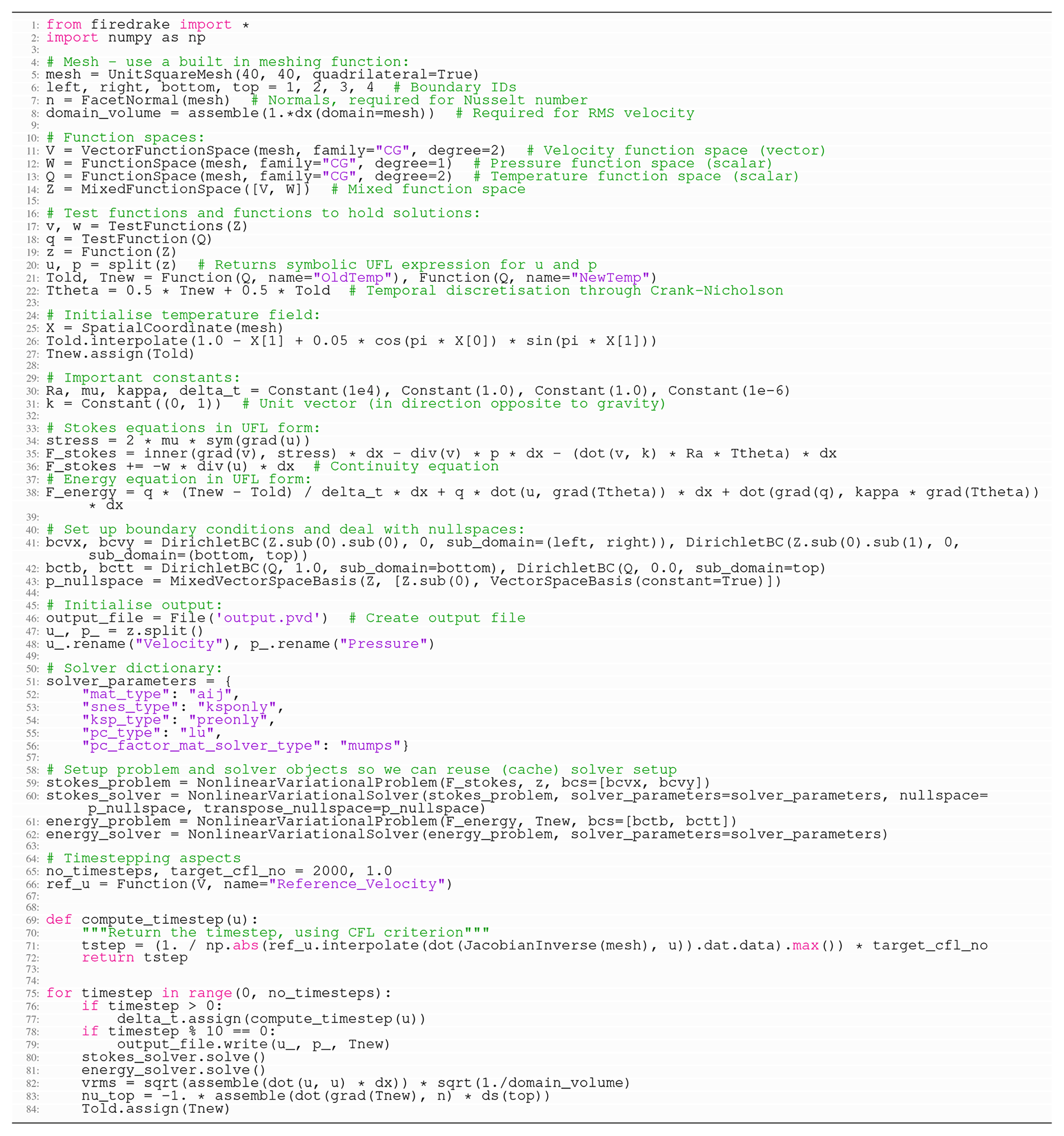
In 84 lines of Python (57 excluding comments and blank lines), we are able to produce a model that can be executed and quantitatively compared to benchmark results from Blankenbach et al. (1989). To do so, we have computed the root mean square (rms) velocity (line 82, using the domain volume specified in line 8) and surface Nusselt number (line 83, using a unit normal vector defined in line 7) at a range of different mesh resolutions and Rayleigh numbers, with results presented in Fig. 1. Results converge towards the benchmark solutions, with increasing resolution. The final steady-state temperature field, at , is illustrated in Fig. 2a.
Figure 2Final steady-state temperature field, in 2-D and 3-D, from Firedrake simulations, designed to match: (a) Case 1a from Blankenbach et al. (1989), with contours spanning temperatures of 0 to 1 at 0.05 intervals. (b) Case 1a is from Busse et al. (1994), with transparent isosurfaces plotted at T=0.3, 0.5 and 0.7.
To further highlight the flexibility of Firedrake, we have also simulated some of these cases using a Q2P1DG discretisation for the Stokes system and a Q1 discretisation for the temperature field. The modifications necessary are minimal: for the former, in line 12, the finite-element family is specified as “DPC”, which instructs Firedrake to use a discontinuous, piecewise linear discretisation for pressure. Note that this choice is distinct from a discontinuous, piecewise bilinear pressure space, which, in combination with Q2 velocities, is not LBB-stable, whereas the Q2P1DG pair is Thieulot and Bangerth (2022). For temperature, the degree specified in line 13 is changed from 2 to 1. Results using a discontinuous linear pressure, at , are presented in Fig. 1c, d, showing a similar trend to those of the Q2Q1 element pair, albeit with rms velocities converging towards benchmark values from above rather than below. Results using a Q1 discretisation for temperature, at , are presented in Fig. 1e, f, converging towards benchmark values with increasing resolution. We find that, as expected, a Q2 temperature discretisation leads to more accurate results, although results converge towards the benchmark solutions from different directions. For the remainder of the examples considered herein, we use a Q2Q1 discretisation for the Stokes system and a Q2 discretisation for temperature.
5.2 Extension: more realistic physics
We next highlight the ease with which simulations can be updated to incorporate more realistic physical approximations. We first account for compressibility under the anelastic liquid approximation (ALA) (e.g. Schubert et al., 2001), simulating a well-established benchmark case from King et al. (2010) (Sect. 5.2.1). We subsequently focus on a case with a more Earth-like approximation of the rheology (Sect. 5.2.2), simulating another well-established benchmark case from Tosi et al. (2015). All cases are set up in an enclosed 2-D Cartesian box with free-slip boundary conditions, with the required changes discussed relative to the base case presented in Sect. 5.1.
5.2.1 Compressibility
Listing 2Difference in Firedrake code required to reproduce compressible ALA cases from King et al. (2010) relative to our base case.
The governing equations applicable for compressible mantle convection, under the ALA, are presented in Appendix A (based on, for example, Schubert et al., 2001). Their weak forms are derived by multiplying these equations by appropriate test functions and integrating over the domain, as we did with their incompressible counterparts in Sect. 4. They differ appreciably from the incompressible approximations that have been utilised thus far, with important updates to all three governing equations. Despite this, the changes required to incorporate these equations, within the UFL and Firedrake, are minimal.
Although King et al. (2010) examined a number of cases, we focus on one illustrative example here, at Ra=105 and a dissipation number Di=0.5. This allows us to demonstrate the ease with which these cases can be configured within Firedrake. The required changes, relative to the base case, are displayed in Listing 2. They can be summarised as follows.
-
Definition and initialisation of additional constants and the 1-D reference state, derived here via an Adams–Williamson equation of state (lines 1–12). In this benchmark example, several of the key constants and parameters required for compressible convection are assigned values of 1 and could be removed. However, to ensure consistency between the governing equations presented in Appendix A and the UFL, we chose not to omit these constants in Listing 2.
-
The UFL for the momentum, mass conservation and energy equations is updated, emphasising once again the resemblance to the mathematical formulation (lines 16–20). The key changes are as follows: (i) the stress tensor is updated to account for a non-zero velocity divergence (line 17), where
Identityrepresents a unit matrix of a given size (2 in this case) anddivrepresents the symbolic divergence of a field. (ii) The Stokes equations are further modified to account for dynamic pressure's influence on buoyancy (final term in line 18). (iii) The mass conservation equation includes the depth-dependent reference density, (line 19), and (iv) the energy equation is updated to incorporate adiabatic heating and viscous dissipation terms (final two terms in line 20). -
Temperature boundary conditions are updated, noting that we are solving for deviatoric temperature rather than the full temperature, which also includes the reference state.
-
In our Stokes solver, we only specify the
transpose_nullspaceoption (as opposed to both thenullspaceandtranspose_nullspaceoptions for our base case): the incorporation of dynamic pressure's impact on buoyancy implies that the (right-hand-side) pressure null space is no longer the same as the (left-hand-side) transpose null space. The transpose null space remains the same space of constant pressure solutions and is used to project out these modes from the initial residual vector to ensure that the linear system is well-posed. The right-hand-side null space now consists of different modes, which can be found through integration. However, this null space is only required for iterative linear solvers in which the modes are projected out from the solution vector at each iteration to prevent its unbounded growth.
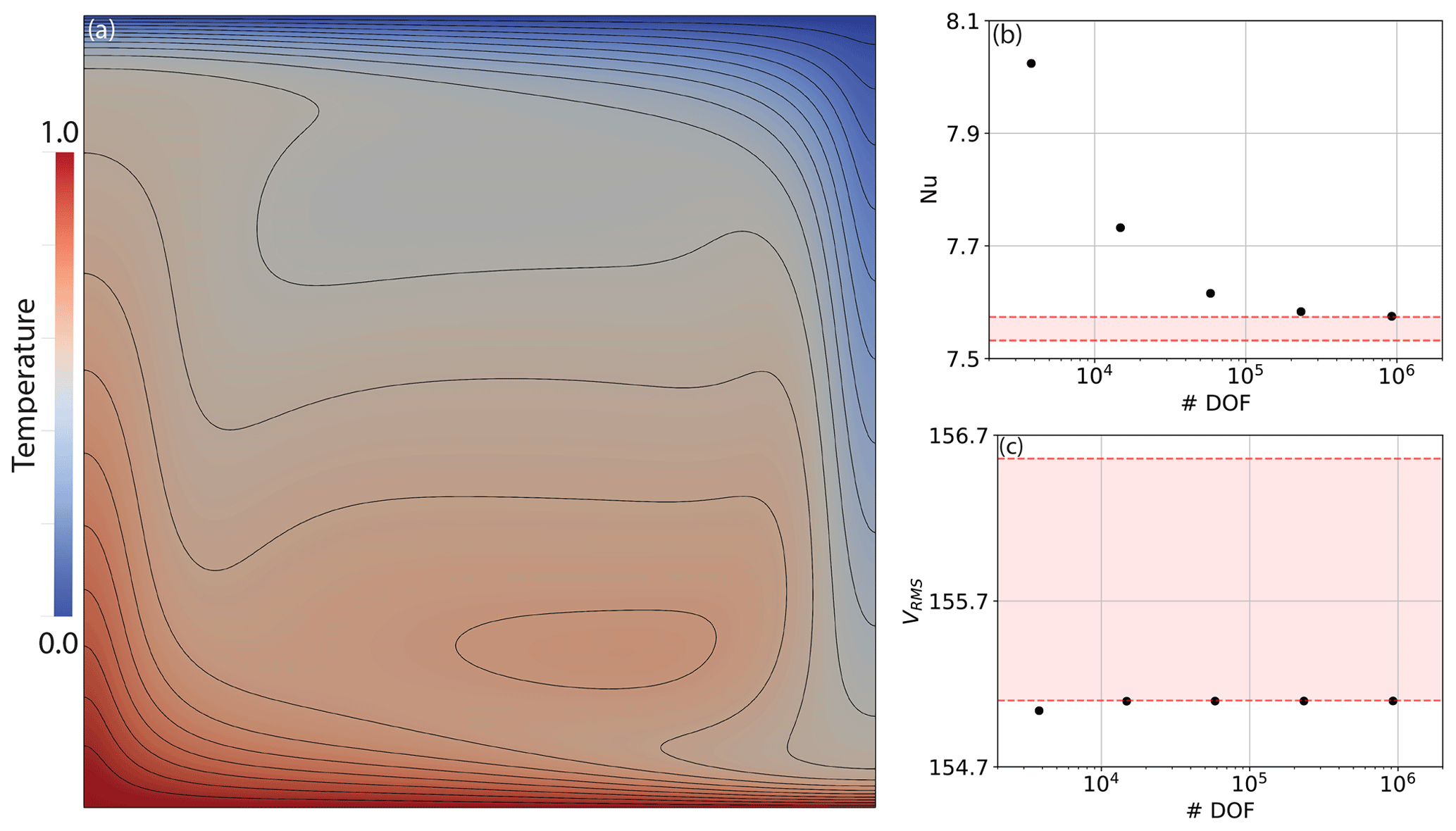
Figure 3Results from Firedrake simulations configured to reproduce the 2‐D compressible benchmark case from King et al. (2010) at Ra=105 and Di=0.5: (a) final steady-state (full) temperature field, with contours spanning temperatures of 0 to 1 at 0.05 intervals; (b) Nusselt number vs. number of pressure and velocity DOFs for a series of uniform, structured meshes; (c) rms velocity vs. number of pressure and velocity DOFs. The range of solutions provided by different codes in the King et al. (2010) benchmark study is bounded by dashed red lines.
We note that, in setting up the Stokes solver as we have, we incorporate the pressure effect on buoyancy implicitly, as advocated by Leng and Zhong (2008). As this term depends on the pressure that we are solving for, an extra term is required in addition to the pressure gradient matrix G in the Jacobian matrix in Eq. (28). The inclusion of in the continuity constraint also means that this term is no longer simply represented by the transpose of G. Such changes are automatically incorporated by Firedrake, highlighting a major benefit of the automatic assembly approach that is utilised. To ensure the validity of our approach, we have computed the rms velocity and Nusselt number at a range of different mesh resolutions, for direct comparison to King et al. (2010), with results presented in Fig. 3, alongside the final steady-state (full) temperature field. As expected, results converge towards the benchmark solutions, with increasing resolution, demonstrating the applicability and accuracy of Firedrake for compressible simulations of this nature.
5.2.2 Viscoplastic rheology
Listing 3Difference in Firedrake code required to reproduce viscoplastic rheology cases from Tosi et al. (2015) relative to our base case.
To illustrate the changes necessary to incorporate a viscoplastic rheology which is more representative of deformation within Earth's mantle and lithosphere, we examine a case from Tosi et al. (2015), a benchmark study intended to form a straightforward extension to Blankenbach et al. (1989). Indeed, aside from the viscosity and reference Rayleigh number (Ra0=102), all other aspects of this case are identical to the case presented in Sect. 5.1. The viscosity field, μ, is calculated as the harmonic mean between a linear component, μlin, and a non-linear plastic component, μplast, which is dependent on the strain rate, as follows:
The linear part is given by an Arrhenius law (the so-called Frank–Kamenetskii approximation):
where γT=ln (ΔμT) and γz=ln (Δμz) are parameters controlling the total viscosity contrast due to temperature and depth respectively. The non-linear component is given by
where μ⋆ is a constant representing the effective viscosity at high stresses and σy is the yield stress. The denominator of the second term in Eq. (38) represents the second invariant of the strain-rate tensor. The viscoplastic flow law (Eq. 36) leads to linear viscous deformation at low stresses and plastic deformation at stresses that exceed σy, with the decrease in viscosity limited by the choice of μ⋆.
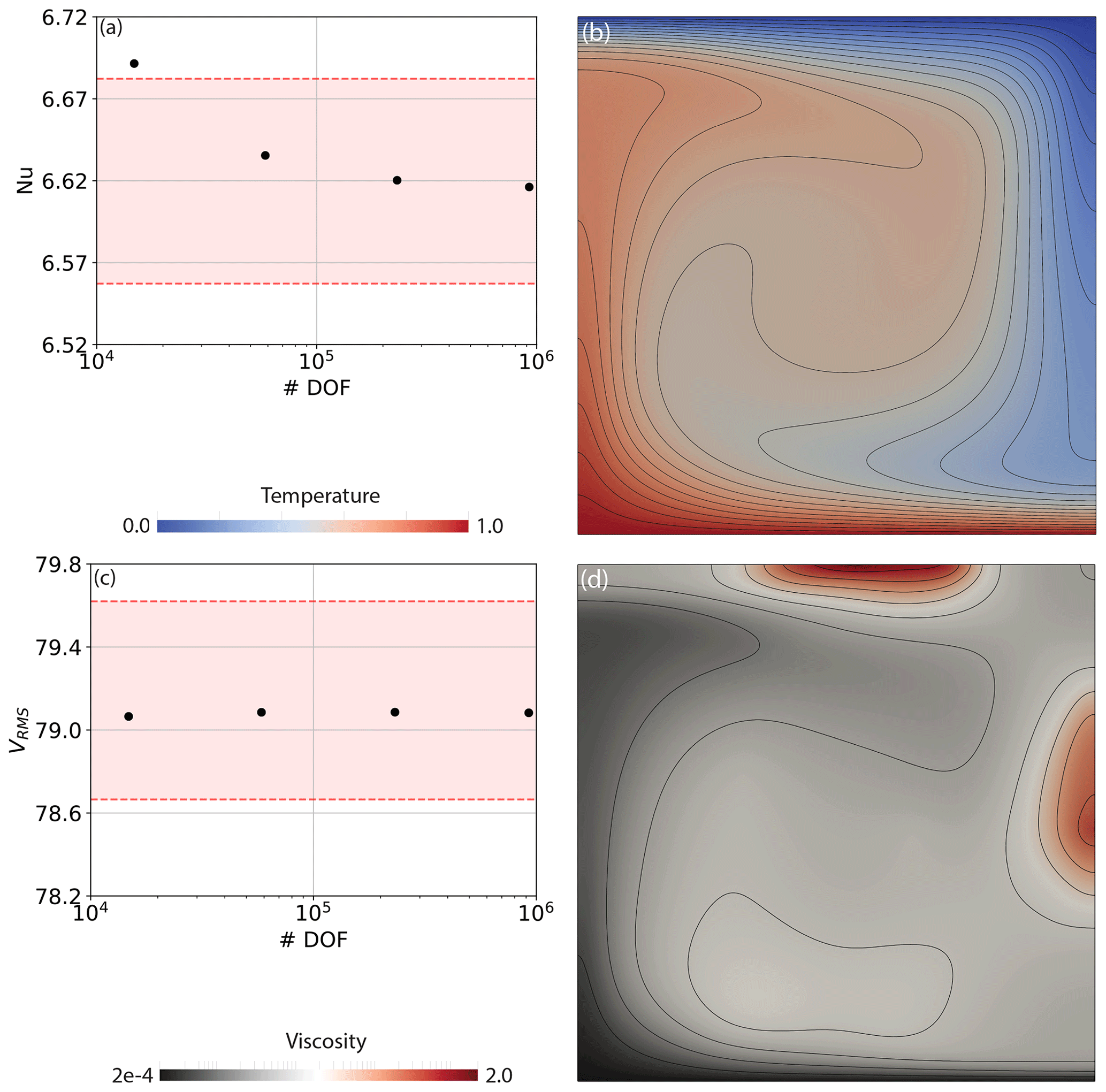
Figure 4Results from the 2‐D benchmark case from Tosi et al. (2015), with a viscoplastic rheology at Ra0=102: (a) Nusselt number vs. number of pressure and velocity DOFs for a series of uniform, structured meshes; (b) final steady-state temperature field, with contours spanning temperatures of 0 to 1, at 0.05 intervals; (c) rms velocity vs. number of pressure and velocity DOFs; (d) final steady-state viscosity field (note logarithmic scale). In panels (a) and (c), the range of solutions provided by different codes in the Tosi et al. (2015) benchmark study is bounded by dashed red lines.
Although Tosi et al. (2015) examined a number of cases, we focus on one here (Case 4: Ra0=102, ΔμT=105, Δμy=10 and ), which allows us to demonstrate how a temperature-, depth- and strain-rate-dependent viscosity is incorporated within Firedrake. The changes required to simulate this case, relative to our base case, are displayed in Listing 3. These are the following.
-
Linear solver options are no longer applicable, given the dependence of viscosity on the flow field, through the strain rate. Accordingly, the solver dictionary is updated to account for the non-linear nature of our Stokes system (lines 2–11). For the first time, we fully exploit the SNES using a set-up based on Newton's method (
"snes_type": "newtonls") with a secant line search over the L2 norm of the function ("snes_linesearch_type": "l2"). As we target a steady-state solution, an absolute tolerance is specified for our non-linear solver ("snes_atol": 1e-10). -
Solver options differ between the (non-linear) Stokes and (linear) energy systems. As such, a separate solver dictionary is specified for solution of the energy equation (lines 13–20). Consistent with our base case, we use a direct solver for solution of the energy equation based on the MUMPS library.
-
Viscosity is calculated as a function of temperature, depth (μlin – line 29) and strain rate (μplast – line 30), using constants specified in lines 25–26. Linear and non-linear components are subsequently combined via a harmonic mean (line 31).
-
Updated solver dictionaries are incorporated into their respective solvers in lines 35 and 36, noting that for this case both the null-space and transpose_nullspace options are provided for the Stokes system, consistent with the base case.
We note that even though the UFL for the Stokes and energy systems remains identical to our base case, assembly of additional terms in the Jacobian, associated with the non-linearity in this system, is once again handled automatically by Firedrake. To compare our results to those of Tosi et al. (2015), we have computed the rms velocity and Nusselt number at a range of different mesh resolutions. These are presented in Fig. 4 and, once again, results converge towards the benchmark solutions, with increasing resolution. Final steady-state temperature and viscosity fields are also illustrated to allow for straightforward comparison to those presented by Tosi et al. (2015), illustrating that viscosity varies by roughly 4 orders of magnitude across the computational domain.
Taken together, our compressible and viscoplastic rheology results demonstrate the accuracy and applicability of Firedrake for problems incorporating a range of different approximations to the underlying physics. They have allowed us to illustrate Firedrake's flexibility: by leveraging the UFL and PETSc, the framework is easily extensible, allowing for straightforward application to scenarios involving different physical approximations, even if they require distinct solution strategies.
5.3 Extension: dimensions and geometry
In this section we highlight the ease with which simulations can be examined in different dimensions and geometries by modifying our basic 2-D case. We primarily simulate benchmark cases that are well-known within the geodynamical community, initially matching the steady-state, isoviscous simulation of Busse et al. (1994) in a 3-D Cartesian domain. There is currently no published community benchmark for simulations in the 2-D cylindrical shell domain. As such, we next compare results for an isoviscous, steady-state case in a 2-D cylindrical shell domain to those of the Fluidity and ASPECT computational modelling frameworks, noting that Fluidity has been carefully validated against the extensive set of analytical solutions introduced by Kramer et al. (2021a) in both cylindrical and spherical shell geometries. Finally, we analyse an isoviscous 3-D spherical shell benchmark case from Zhong et al. (2008). Once again, the changes required to run these cases are discussed relative to our base case (Sect. 5.1) unless noted otherwise.
5.3.1 3-D Cartesian domain
We first examine and validate our set-up in a 3-D Cartesian domain for a steady-state, isoviscous case – specifically Case 1a from Busse et al. (1994). The domain is a box of dimensions . The initial temperature distribution, chosen to produce a single ascending and descending flow, at and respectively is prescribed as
where A=0.2 is the amplitude of the initial perturbation. We note that this initial condition differs from that specified in Busse et al. (1994), through the addition of boundary layers at the bottom and top of the domain (through the erf terms), although it more consistently drives solutions towards the final published steady-state results. Boundary conditions for temperature are T=0 at the surface (z=1) and T=1 at the base (z=0), with insulating (homogeneous Neumann) sidewalls. No‐slip velocity boundary conditions are specified at the top surface and base of the domain, with free‐slip boundary conditions on all sidewalls. The Rayleigh number is .

Listing 4Changes required to reproduce a 3-D Cartesian case from Busse et al. (1994) relative to Listing 1.
In comparison to Listing 1, the changes required to simulate this case, using Q2Q1 elements for velocity and pressure, are minimal. The key differences, summarised in Listing 4, are the following.
-
The creation of the underlying mesh (lines 1–5), which we generate by extruding a 2-D quadrilateral mesh in the z direction to a layered 3-D hexahedral mesh. Our final mesh has elements in the x, y and z directions respectively (noting that the default value for layer height is ). For extruded meshes, top and bottom boundaries are tagged by
topandbottomrespectively, whilst boundary markers from the base mesh can be used to set boundary conditions on the relevant side of the extruded mesh. We note that Firedrake exploits the regularity of extruded meshes to enhance performance. -
Specification of the initial condition for temperature, following Eq. (39), updated values for Ra and definition of the 3-D unit vector (lines 9–11).
-
The inclusion of Python dictionaries that define iterative solver parameters for the Stokes and energy systems (lines 15–47). Although direct solves provide robust performance in the 2-D cases examined above, in 3-D the computational (CPU and memory) requirements quickly become intractable. PETSc's
fieldsplitpc_typeprovides a class of preconditioners for mixed problems that allows one to apply different preconditioners to different blocks of the system. This opens up a large array of potential solver strategies for the Stokes saddle point system (e.g. many of the methods described in May and Moresi, 2008). Here we configure the Schur complement approach as described in Sect. 4.3. We note that thisfieldsplitfunctionality can also be used to provide a stronger coupling between the Stokes system and energy equation in strongly non-linear problems, where the Stokes and energy systems are solved together in a single Newton solve that is decomposed through a series of preconditioner stages.The
fieldsplit_0entries configure solver options for the first of these blocks, the K matrix. The linear systems associated with this matrix are solved using a combination of the conjugate gradient method (cg, line 23) and an algebraic multigrid preconditioner (gamg, line 27). We also specify two options (gamg_thresholdandgamg_square_graph) that control the aggregation method (coarsening strategy) in the GAMG preconditioner, which balance the multigrid effectiveness (convergence rate) with coarse grid complexity (cost per iteration) (Balay et al., 2021a).The
fieldsplit_1entries contain solver options for the Schur complement solve itself. As explained in Sect. 4.3, we do not have explicit access to the Schur complement matrix, GTK−1G, but can compute its action on any vector, at the cost of afieldsplit_0solve with the K matrix, which is sufficient to solve the system using a Krylov method. However, for preconditioning, we do need access to the values of the matrix or its approximation. For this purpose we approximate the Schur complement matrix with a mass matrix scaled by viscosity, which is implemented inMassInvPC(line 35) with the viscosity provided through the optionalappctxargument in line 71. This is a simple example of Firedrake's powerful programmable preconditioner interface, which, in turn, connects with the Python preconditioner interface of PETSc (line 34). In more complex cases the user can specify their own linear operator in the UFL that approximates the true linear operator but is easier to invert. TheMassInvPCpreconditioner step itself is performed through a linear solve with the approximate matrix with options prefixed withMp_to specify a conjugate gradient solver with symmetric SOR (SSOR) preconditioning (lines 36–38). Note that PETSc'ssorpreconditioner type, specified in line 38, defaults to the symmetric SOR variant. Since this preconditioner step now involves an iterative solve, the Krylov method used for the Schur complement needs to be of a flexible type, and we specifyfgmresin line 32.Specification of the matrix type
matfree(line 16) for the combined system ensures that we do not explicitly assemble its associated sparse matrix, instead computing the matrix–vector multiplications required by the Krylov iterations as they arise. For example, the action of the sub-matrix G on a sub-vector can be evaluated as (cf. Eqs. 28, 30)which is assembled by Firedrake directly from the symbolic expression into a discrete vector. Again, for preconditioning in the K-matrix solve, we need access to matrix values, which is achieved using
AssembledPC. This explicitly assembles the K matrix by extracting relevant terms from theF_Stokesform.Finally, the energy solve is performed through a combination of the GMRES (
gmres) Krylov method and SSOR preconditioning (lines 42–47). For all iterative solves we specify a convergence criterion based on the relative reduction of the preconditioned residual (ksp_rtol: lines 24, 33, 36 and 46). -
Velocity boundary conditions, which must be specified along all six faces, are modified in lines 51–53, with temperature boundary conditions specified in line 54.
-
Generating near-null-space information for the GAMG preconditioner (lines 58–66), consisting of three rotational (
x_rotV,y_rotV,z_rotV) and three translational (nns_x,nns_y,nns_z) modes, as outlined in Sect. 4.3. These are combined in the mixed function space in line 66. -
Updating of the Stokes problem (line 70) to account for additional boundary conditions and the Stokes solver (line 71) to include the near-null-space options defined above, in addition to the optional
appctxkeyword argument that passes the viscosity through to ourMassInvPCSchur complement preconditioner. Energy solver options are also updated relative to our base case (lines 72–73), using the dictionary created in lines 42–47.

Figure 5Results from 3‐D isoviscous simulations in Firedrake, configured to reproduce benchmark results from Case 1a of Busse et al. (1994): (a) Nusselt number vs. number of pressure and velocity DOFs at for a series of uniform, structured meshes; (b) rms velocity vs. number of pressure and velocity DOFs. Benchmark values are denoted by dashed red lines.
Listing 5Difference in Firedrake code required to reproduce the isoviscous case in a 2-D cylindrical shell domain.
Our model results can be validated against those of Busse et al. (1994). As with our previous examples, we compute the Nusselt number and rms velocity at a range of different mesh resolutions, with results presented in Fig. 5. We find that results converge towards the benchmark solutions with increasing resolution, as expected. The final steady-state temperature field is illustrated in Fig. 2b.
5.3.2 2-D cylindrical shell domain
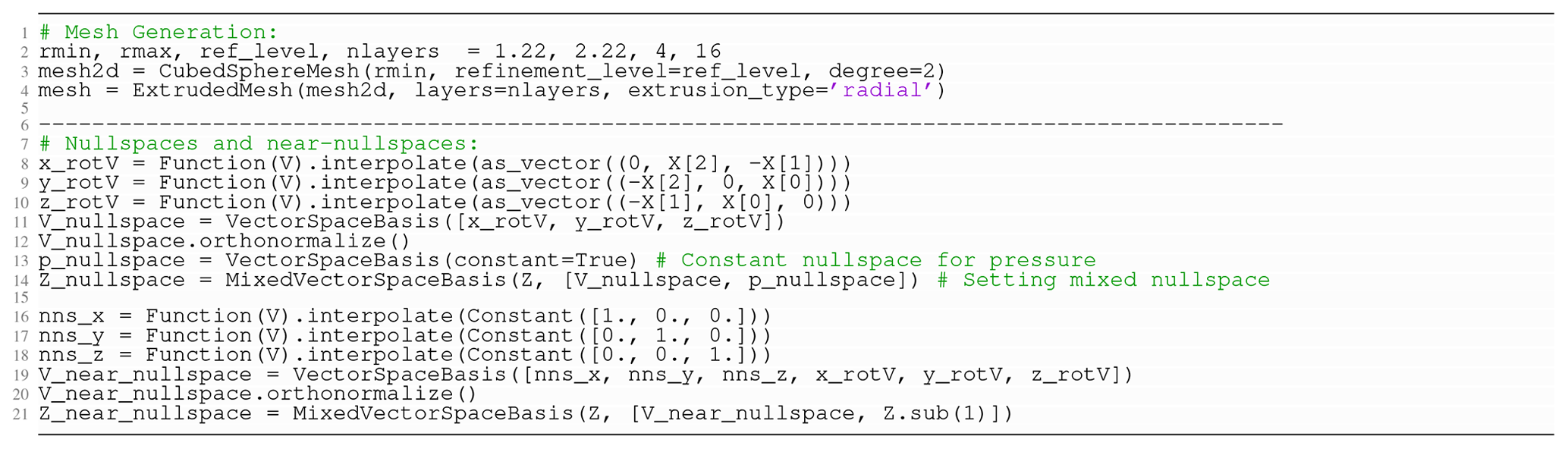
We next examine simulations in a 2-D cylindrical shell domain, defined by the radii of the inner (rmin) and outer (rmax) boundaries. These are chosen such that the non-dimensional depth of the mantle is and the ratio of the inner and outer radii is , thus approximating the ratio between the radii of Earth's surface and the core–mantle boundary (CMB). Specifically, we set rmin=1.22 and rmax=2.22. The initial temperature distribution, chosen to produce four equidistant plumes, is prescribed as
where A=0.02 is the amplitude of the initial perturbation. Boundary conditions for temperature are T=0 at the surface (rmax) and T=1 at the base (rmin). Free‐slip velocity boundary conditions are specified on both boundaries, which we incorporate weakly through the Nitsche approximation (see Sect. 4.1). The Rayleigh number is .

Figure 6(a, b) Nusselt number/rms velocity vs. number of pressure and velocity DOFs at for a series of uniform, structured meshes in a 2-D cylindrical shell domain. High-resolution, adaptive mesh results from the Fluidity computational modelling framework (Davies et al., 2011) are delineated by dashed red lines, with results from ASPECT delineated by dotted red lines (Bangerth et al., 2020); (c) final steady-state temperature field, with contours spanning temperatures of 0 to 1, at intervals of 0.05.
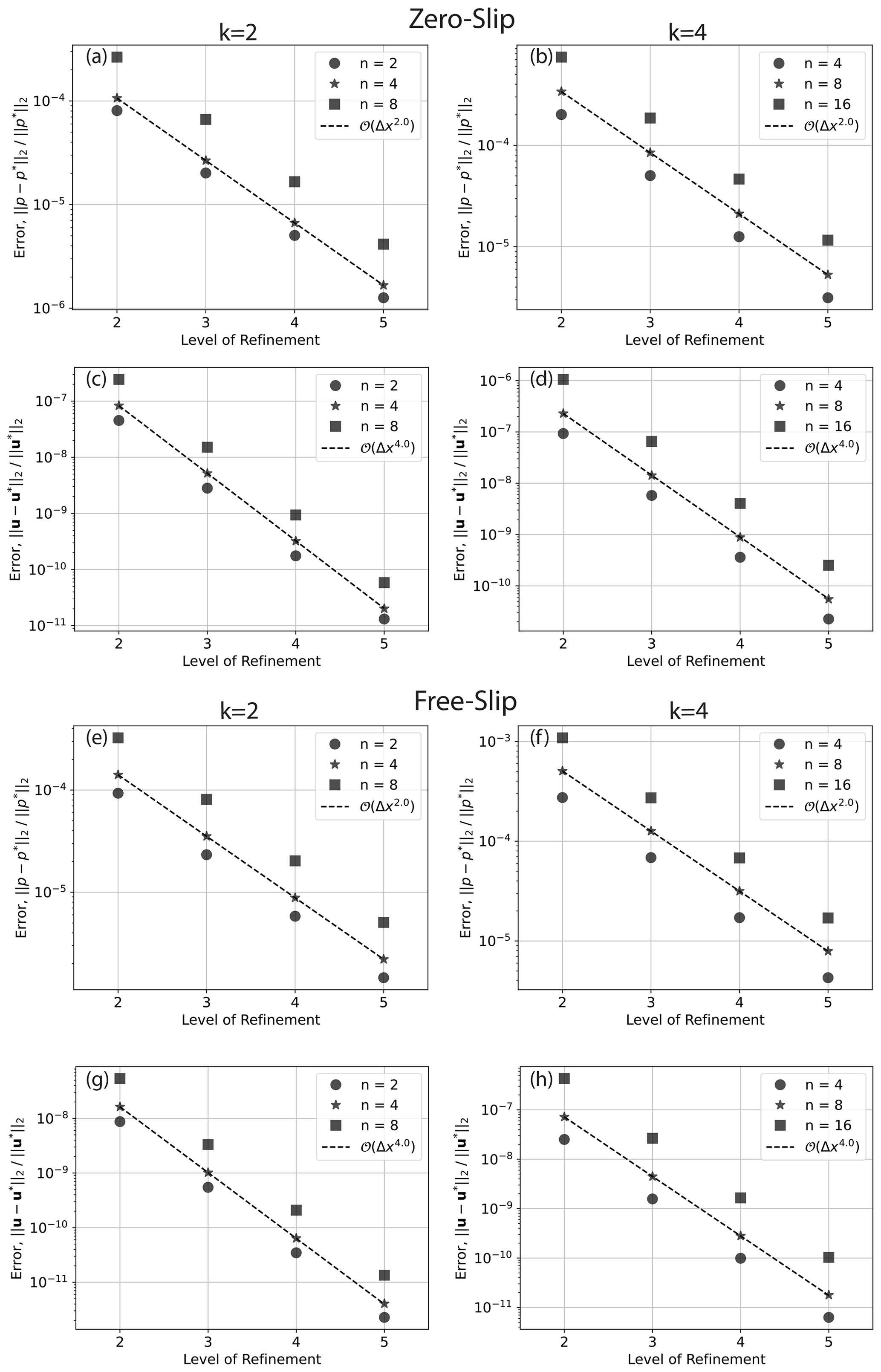
Figure 7Convergence for 2-D cylindrical shell cases with zero-slip (a–d) and free-slip (e–h) boundary conditions, driven by smooth forcing at a series of different wave numbers, n, and different polynomial orders of the radial dependence, k, as indicated in the legend (see Kramer et al., 2021a, for further details). Convergence rate is indicated by dashed lines, with the order of convergence provided in the legend. For the cases plotted, the series of meshes start at refinement level 1, where the mesh consists of 1024 divisions in the tangential direction and 64 radial layers. At each subsequent level the mesh is refined by doubling resolution in both directions.
With a free-slip boundary condition on both boundaries, one can add an arbitrary rotation of the form to the velocity solution (i.e. this case incorporates a velocity null space as well as a pressure null space). As noted in Sect. 4, these lead to null modes (eigenvectors) for the linear system, rendering the resulting matrix singular. In preconditioned Krylov methods, these null modes must be subtracted from the approximate solution at every iteration (e.g. Kramer et al., 2021a), which we illustrate through this example. The key changes required to simulate this case, displayed in Listing 5, are the following.
-
Mesh generation: we generate a circular manifold mesh (with 256 elements in this example) and extrude in the radial direction, using the optional keyword argument
extrusion_type, forming 64 layers (lines 2–4). To better represent the curvature of the domain and ensure accuracy of our quadratic representation of velocity, we approximate the curved cylindrical shell domain quadratically, using the optional keyword argumentdegree=2 (see Sect. 4 for further details). -
The unit vector, , points radially in the direction opposite to gravity, as defined in line 10. The temperature field is initialised using Eq. (41) in line 11.
-
Boundary conditions are no longer aligned with Cartesian directions. We use the Nitsche method (see Sect. 4.1) to impose our free-slip boundary conditions weakly (lines 15–27). The fudge factor in the interior penalty term is set to 100 in line 16, with Nitsche-related contributions to the UFL added in lines 24–27. Note that, for extruded meshes in Firedrake,
ds_tbdenotes an integral over both the top and bottom surfaces of the mesh (ds_tandds_bdenote integrals over the top or bottom surface of the mesh respectively).FacetAreaandCellVolumereturn respectively Af and required by Eq. (17). Given that velocity boundary conditions are handled weakly through the UFL, they are no longer passed to the Stokes problem as a separate option (line 46). Note that, in addition to the Nitsche terms, the UFL for the Stokes equations now also includes boundary terms associated with the pressure gradient and velocity divergence terms, which were omitted in Cartesian cases (for details, see Sect. 4.1). -
We define the rotational null space for velocity and combine this with the pressure null space in the mixed finite-element space Z (lines 30–34). Constant and rotational near-null spaces, utilised by our GAMG preconditioner, are also defined in lines 37–41, with this information passed to the solver in line 46. Note that iterative solver parameters, identical to those presented in the previous example, are used (see Sect. 5.3.1).
Listing 6Difference in Firedrake code required to reproduce 3-D spherical shell benchmark cases from Zhong et al. (2008).
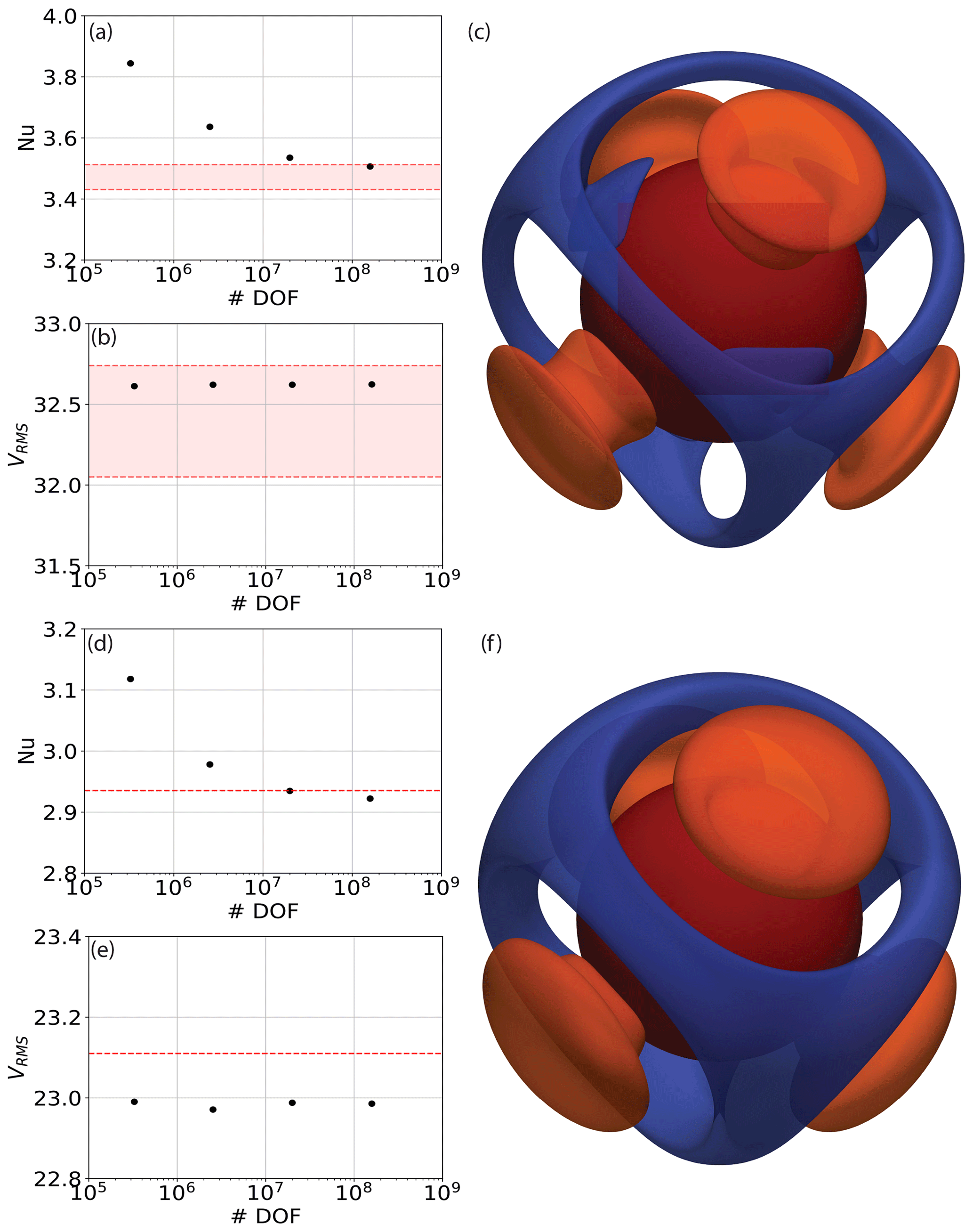
Figure 8(a, b) Nusselt number/rms velocity vs. number of pressure and velocity DOFs, designed to match an isoviscous 3-D spherical shell benchmark case at for a series of uniform, structured meshes. The range of solutions predicted in previous studies is bounded by dashed red lines (Bercovici et al., 1989; Ratcliff et al., 1996; Yoshida and Kageyama, 2004; Stemmer et al., 2006; Choblet et al., 2007; Tackley, 2008; Zhong et al., 2008; Davies et al., 2013; Liu and King, 2019). (c) Final steady-state temperature field highlighted through isosurfaces at temperature anomalies (i.e. away from the radial average) of (blue) and T=0.15 (orange), with the core–mantle boundary at the base of the spherical shell marked by a red surface; (d–f) as in (a)–(c) but for a temperature-dependent viscosity case, with thermally induced viscosity contrasts of 102. Fewer codes have published predictions for this case, but results of Zhong et al. (2008) are marked by dashed red lines for comparison.
Our predicted Nusselt numbers and rms velocities converge towards those of existing codes with increasing resolution (Fig. 6), demonstrating the accuracy of our approach. To further assess the validity of our set-up, we have confirmed the accuracy of our solutions to the Stokes system in this 2-D cylindrical shell geometry, through comparisons to analytical solutions from Kramer et al. (2021a) for both zero-slip and free-slip boundary conditions. These provide a suite of solutions based upon a smooth forcing term at a range of wave numbers n, with radial dependence formed by a polynomial of arbitrary order k. We study the convergence of our Q2Q1 discretisation with respect to these solutions. Convergence plots are illustrated in Fig. 7. We observe super-convergence for the Q2Q1 element pair at fourth and second order, for velocity and pressure respectively, with both zero-slip and free-slip boundary conditions, which is higher than the theoretical (minimum) expected order of convergence of 3 for velocity and 2 for pressure (we note that super-convergence was also observed in Zhong et al., 2008, and Kramer et al., 2021a). Cases with lower wave number, n, show smaller relative error than those at higher n, as expected. The same observation holds for lower and higher polynomial orders, k=2 and k=4, for the radial density profile. To demonstrate the flexibility of Firedrake, we have also run comparisons against analytical solutions using a (discontinuous) delta-function forcing. In this case, convergence for the Q2Q1 discretisation (Fig. A1) drops to 1.5 and 0.5 for velocity and pressure respectively. However, by employing the Q2P1DG finite-element pair, we observe convergence at 3.5 and 2.0 (Fig. A2). Consistent with Kramer et al. (2021a), this demonstrates that the continuous approximation of pressure can lead to a reduced order of convergence in the presence of discontinuities, which can be overcome using a discontinuous pressure discretisation. Python scripts for these analytical comparisons can be found in the repository accompanying this paper.
5.3.3 3-D spherical shell domain
We next move into a 3-D spherical shell geometry, which is required to simulate global mantle convection. We examine a well-known isoviscous community benchmark case (e.g. Bercovici et al., 1989; Ratcliff et al., 1996; Zhong et al., 2008; Davies et al., 2013), at a Rayleigh number of , with free-slip velocity boundary conditions. Temperature boundary conditions are set to 1 at the base of the domain (rmin=1.22) and 0 at the surface (rmax=2.22), with the initial temperature distribution approximating a conductive profile with superimposed perturbations triggering tetrahedral symmetry at spherical harmonic degree l=3 and order m=2 (see Zhong et al., 2008, for further details).
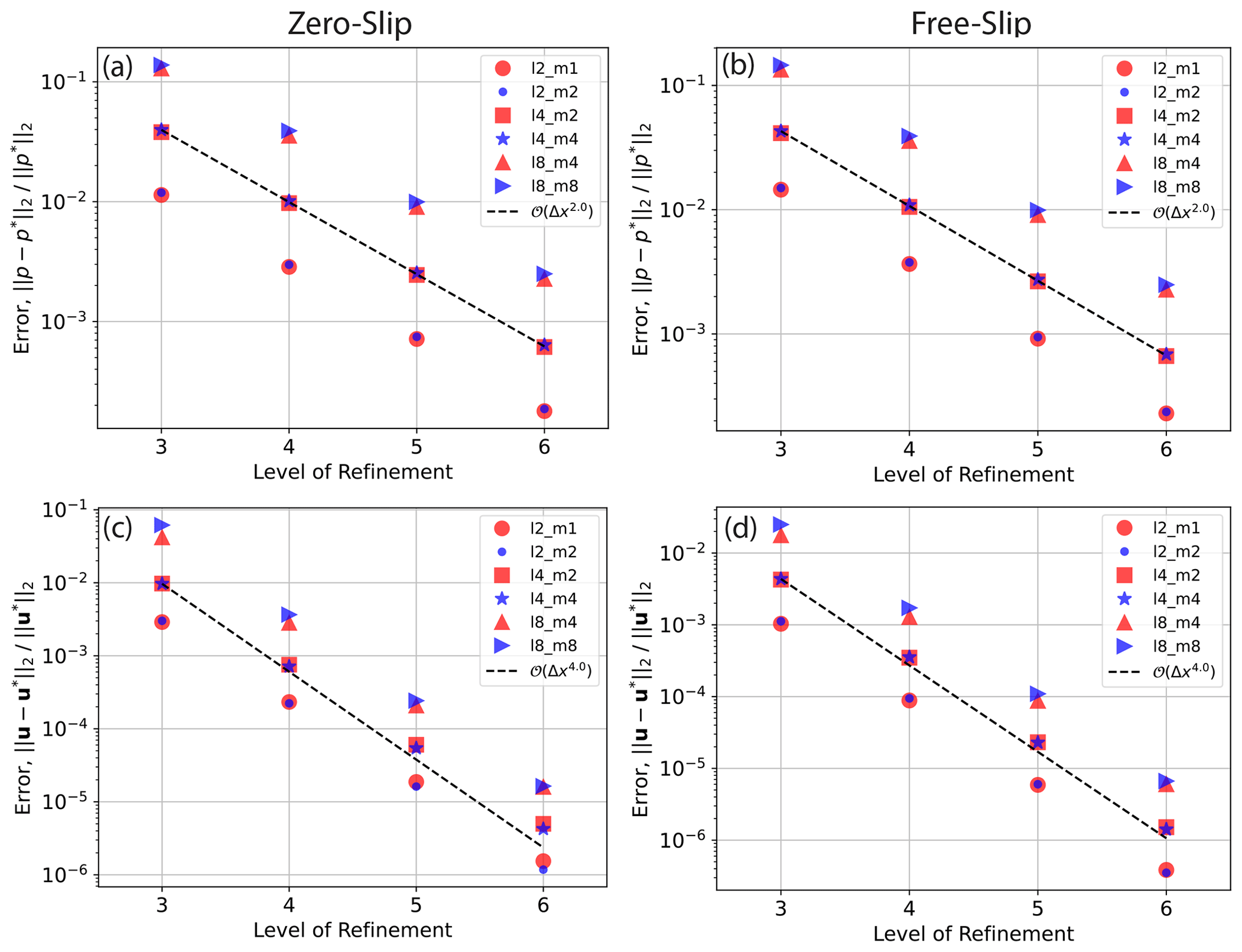
Figure 9Convergence of velocity and pressure for 3-D spherical shell cases with zero-slip and free-slip boundary conditions for perturbations at a range of spherical harmonic degrees l and orders m. Note that all cases with a smooth forcing are run at . Refinement level 3 corresponds to the level specified for our cubed sphere mesh, comprising 386 elements in the tangential direction, which is extruded radially to eight layers. Resolution is doubled in all directions at subsequent refinement levels.
As illustrated in Listing 6, when compared to the 2-D cylindrical shell case examined in Sect. 5.3.2, the most notable change required to simulate this 3-D case is the generation of the underlying mesh. We use Firedrake's built-in CubedSphereMesh and extrude it radially through 16 layers, forming hexahedral elements. As with our cylindrical shell example, we approximate the curved spherical domain quadratically using the optional keyword argument degree=2. Further required changes, highlighted in Listing 6, relate to 3-D extensions of the velocity null space and the near-null spaces required by the GAMG preconditioner, all of which are simple. We do not show the changes associated with extending the radial unit vector to 3-D or the initial condition for temperature, given that they are straightforward, although, as with all examples, a complete Python script for this case can be found in the repository accompanying this paper.
Despite the simplicity of our set-up, the accuracy of our approach is confirmed via comparison of both Nusselt numbers and rms velocities to those of previous studies (e.g. Bercovici et al., 1989; Ratcliff et al., 1996; Yoshida and Kageyama, 2004; Stemmer et al., 2006; Choblet et al., 2007; Tackley, 2008; Zhong et al., 2008; Davies et al., 2013; Liu and King, 2019). For completeness, the final steady-state temperature field is illustrated in Fig. 8c. Furthermore, in line with our 2-D cases, we have confirmed the accuracy of our Stokes solver for both zero-slip and free-slip boundary conditions in a 3-D spherical shell geometry through comparisons to analytical solutions from Kramer et al. (2021a), which provide solutions based upon a smooth forcing term at a range of spherical harmonic degrees, l, and orders, m, with radial dependence formed by a polynomial of arbitrary order k. As with our 2-D cases, we observe super-convergence for the Q2Q1 element pair at fourth and second order for velocity and pressure respectively, with both zero-slip and free-slip boundary conditions (Fig. 9).
This section has allowed us to highlight a number of Firedrake's benefits over other codes: (i) the ease with which simulations can be examined in different geometries, with minimal changes to the Python code, facilitated by Firedrake's built-in mesh generation utilities and extrusion functionality; (ii) the ease with which iterative solver configurations and preconditioners can be updated and tested, including scenarios incorporating multiple null spaces, facilitated by Firedrake's fully programmable solver interface, alongside its customisable preconditioner interface, both of which are seamlessly coupled to PETSc; (iii) the convergence properties of our finite-element system in geometries that are representative of Earth's mantle. Taken together, these confirm Firedrake's suitability for simulations of global mantle dynamics, as will be further highlighted in Sect. 7.
We assess parallel scalability using a 3-D spherical shell case similar to that presented in Sect. 5.3.3, albeit incorporating a temperature-dependent viscosity, following the relation
where E is a parameter that controls the temperature dependence of viscosity. In the example considered – Case A4 from Zhong et al. (2008) – we set E=ln (100), leading to thermally induced viscosity contrasts of 102 across the computational domain. For completeness, our steady-state results, highlighting the consistency of our results for this case with the predictions of Zhong et al. (2008), are displayed in Fig. 8, although for the purposes of parallel scaling analyses, we run simulations for 20 time steps only.
We focus on weak scaling, where the problem size and the number of processing cores are simultaneously increased. Cases are examined on 24, 192, 1536 and 12 288 cores, maintaining 4096 elements per core and ensuring a constant element aspect ratio across all resolutions examined. Simulations were examined on the Gadi supercomputer at the National Computational Infrastructure (NCI) in Australia, using compute nodes with 2×24 core Intel Xeon Platinum 8274 (Cascade Lake) 3.2 GHz CPUs and 192 GB RAM per node. Linking the nodes is the latest-generation HDR InfiniBand technology in a Dragonfly+ topology, capable of transferring data at up to 200 GB s−1.
The most challenging aspect of weak parallel scaling is solver performance as the problem size increases. Whilst the amount of computation in equation assembly typically scales linearly with the number of DOFs – before taking parallel aspects such as communication into account – solver scaling is generally worse. In the case of iterative solvers, this is due to a deterioration in the conditioning of the matrix, driving an increase in the number of iterations required for convergence. As a result, even if the cost per iteration scales linearly, the overall cost will not. This implies that, for weak scaling, the amount of work per core may increase rapidly despite the number of DOFs per core remaining consistent.

Figure 10Weak scaling analyses for a 20 time-step, temperature-dependent viscosity, spherical shell simulation with free-slip boundary conditions: (a) mean number of iterations per time step for energy (blue stars), pressure (red squares) and velocity (green circles) solves respectively; (b) time spent in assembly of finite-element systems; (c) time spent setting up the algebraic multigrid preconditioner; (d) time spent solving the Schur complement (Stokes) system; (e) cost per velocity solve iterations; (f) total simulation time, which closely mimics the Schur complement solution time.
The deterioration in conditioning is intimately related to the fact that an increase in resolution increases the ratio between the smallest and largest resolvable length scales. For elliptic operators, like the viscosity matrix K, the condition number scales with the square of that ratio (e.g. Kramer et al., 2010). Multigrid approaches, which separate smaller and larger length scales on a hierarchy of fine to coarse meshes, are commonly used to address this problem, which motivates the choice of the algebraic multigrid preconditioner, GAMG, used here. Such approaches aim to maintain a constant or only slowly increasing number of iterations and, thus, a near-linear scaling of the overall cost as the problem size increases. This can be a challenge however, as, for instance, an increase in resolution will require more multigrid levels, which will lead to an increased set-up time and cost per iteration. In practice, when configuring the multigrid method, a compromise needs to be found between the effectiveness of a multigrid in limiting the number of iterations and not allowing the set-up and costs per iteration to grow too rapidly. The two options, gamg_threshold and gamg_square_graph, specified in our solver set-up ensure a balance between multigrid effectiveness and coarse grid complexity.
A breakdown of key parallel scaling results is presented in Fig. 10. Panel (a) displays the average number of iterations per solve over the 20 time steps. We find that the number of pressure (the Schur complement solve: fieldsplit_1) and energy solve iterations remains flat (12 and ∼10.5 respectively), whilst the number of velocity solve iterations (inversion of the matrix K, using the GAMG preconditioner: fieldsplit_0) increases only slowly, from ∼41 to ∼51, over a greater than 3 order of magnitude increase in problem size and number of processor cores. This demonstrates algorithmic scalability on up to 12 288 cores and elements (which corresponds to velocity and pressure degrees of freedom).
Parallel scalability can also be assessed by analysing the growth in CPU time of the dominant components of our problem: assembly of finite-element systems (Fig. 10b), set-up of the algebraic multigrid (GAMG) preconditioner (Fig. 10c), and time spent solving the Schur complement system (Fig. 10d). We find that the assembly time is a negligible fraction of this problem. The set-up time for our GAMG preconditioner grows from ∼240 s on 24 cores to ∼470 s on 12 288 cores. This is understandable given the high communication costs associated with setting up various multigrid levels, particularly for problems incorporating null spaces and near-null spaces, as is the case here. We note, however, that this is not a concern: as a fraction of the entire solution time for the Schur complement solve (Fig. 10d), GAMG set-up remains small. We do observe an increase in time required for solution of the Schur complement (Stokes solve) from ∼6500 s on 24 cores to ∼12 100 s on 12 288 cores. This results primarily from the minor increase in the number of velocity solve iterations and the increased cost per iteration (Fig. 10e), which rises from 155 s on 24 cores to 225 s on 12 288 cores, reflecting costs associated with increasing the number of multigrid levels for higher-resolution problems. The total time spent in running this problem mirrors the time spent in solving the Schur complement system (Fig. 10f), indicating where future optimisation efforts should be directed.
In this section, we demonstrate application of Firedrake to a time-dependent simulation of global mantle convection in a 3-D spherical shell geometry, at a realistic Rayleigh number. We assume a compressible mantle, under the ALA, and a temperature-, depth-, and strain-rate-dependent rheology, in line with the viscoplastic case analysed in Sect. 5.2.2. Viscosity increases below the mantle transition zone and we include a brittle-failure-type yield-stress law, ensuring that yielding concentrates at shallow depths. As with the examples provided above, calculations are performed using a hexahedral Q2Q1 element pair for velocity and pressure. We use a Q2 discretisation for temperature and, given the increased importance of advection at higher Rayleigh numbers, incorporate stabilisation through a streamline upwinding scheme, following Donea and Huerta (2003). We employ a cubed sphere mesh with 98 304 elements on each spherical surface and extrude it radially through 64 layers, with spacing reduced adjacent to the top and bottom boundaries of the domain. This results in a problem with velocity and pressure degrees of freedom and temperature degrees of freedom. Our solution strategy for the Stokes equations is similar to the spherical shell examples presented above, albeit exploiting PETSc's SNES functionality using a set-up based on Newton's method to handle the non-linearity in the system. The solution strategy for the energy equation is identical to the previous example.
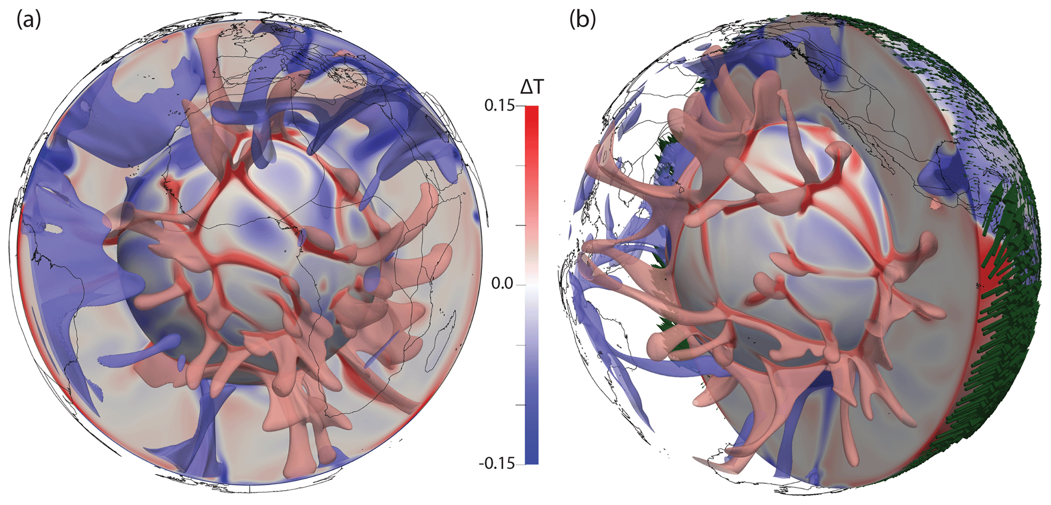
Figure 11Present-day thermal structure, predicted from our global mantle convection simulation where the geographic distribution of heterogeneity is dictated by 230 Myr of imposed plate motion history (Müller et al., 2016). Each image includes a radial surface at r=1.25 (i.e. immediately above the core–mantle boundary), a cross section and transparent isosurfaces at temperature anomalies (i.e. away from the radial average) of (blue) and T=0.075 (red), highlighting the location of downwelling slabs and upwelling mantle plumes (below r=2.13) respectively. Continental boundaries provide geographic reference. Panel (a) provides an Africa-centred view, with panel (b) centred on the Pacific Ocean and including (green) glyphs at the surface highlighting the imposed plate velocities.
We achieve a (basally heated) Rayleigh number of 7.5×10⁷ in the asthenosphere, which is comparable to estimates of Earth's mantle (e.g. Davies, 1999) and also includes internal heating at a non-dimensional heating rate of 10. The simulation is spun up with free-slip and isothermal boundaries at both surfaces. After the model reaches a quasi-steady state (i.e. when the surface and basal Nusselt numbers both change by less than 0.1 % over 10 consecutive time steps), surface velocities are assimilated through a kinematic boundary condition, according to 230 Myr of plate motion histories (Müller et al., 2016), using the Python interface to GPlates (e.g. Gurnis et al., 2012; Müller et al., 2018). Our simulation then runs forward towards the present day. This case is therefore similar to the simulations examined when addressing questions from the very frontiers of geodynamical research, albeit incorporating a more representative treatment of mantle and lithosphere rheology (e.g. Schuberth et al., 2009; Davies and Davies, 2009; Davies et al., 2012; Bower et al., 2013; Hassan et al., 2015; Nerlich et al., 2016; Rubey et al., 2017; Koelemeijer et al., 2018; Ghelichkhan et al., 2018; Flament et al., 2022). The simulation was executed across 1344 CPUs, on the same architecture as outlined above, and took ∼92 h.
Our results are illustrated in Fig. 11. We find that the present-day upper-mantle convective planform is dominated by strong downwellings in regions of plate convergence. In the middle mantle, cold downwellings are prominent beneath North America and South-East Asia, whilst remnants of older subduction are visible above the core–mantle boundary. The location of hot upwelling material is strongly modulated by these downwellings, with upwelling plumes concentrating in two clusters beneath the African continent and the central Pacific Ocean (i.e. away from regions that have experienced subduction over the past 150 Myr or so). The cluster of plumes in the Pacific is reasonably circular, whilst those beneath Africa extend in a NW–SE-trending structure, which to the north curves eastward under Europe and to the south extends into the Indian Ocean.
Further analysis of this proof-of-concept simulation is beyond the scope of this study. However, when combined with the benchmark and parallel scaling analyses presented above, our model predictions, which are consistent with those from a number of previous studies (e.g. Bunge et al., 2002; Davies et al., 2012; Bower et al., 2013; Davies et al., 2015a), confirm Firedrake's applicability for time-dependent global mantle dynamics simulations of this nature.
Firedrake is a next-generation automated system for solving variational problems using the finite-element method (e.g. Rathgeber et al., 2016; Gibson et al., 2019). It has a number of features that are ideally suited to simulating geophysical fluid dynamics problems, as exemplified by its use in application areas such as coastal ocean modelling (Kärnä et al., 2018), numerical weather prediction (Shipton et al., 2018) and glacier flow modelling (Shapero et al., 2021). The focus of this paper has been to demonstrate Firedrake's applicability for geodynamical simulation, with an emphasis on global mantle dynamics. To do so, we have presented, analysed and validated Firedrake against a number of benchmark and analytical cases of systematically increasing complexity, building towards a time-dependent global simulation at realistic convective vigour.
To introduce its core components and illustrate the elegance of setting up and validating a geodynamical model in Firedrake, we started with a simple, incompressible, isoviscous case in an enclosed 2-D Cartesian box. Setting up this problem was straightforward, requiring only a weak formulation of the governing equations for specification in the UFL, together with a mesh, initial and boundary conditions, and appropriate discrete function spaces. We utilised Firedrake's built-in meshing functionality and default direct solver options and demonstrated the framework's accuracy for simulations of this nature: in only 56 lines of Python (excluding comments and blank lines), we reproduced results from the well-established benchmark study of Blankenbach et al. (1989).
Representative simulations of mantle and lithosphere dynamics, however, incorporate more complicated physics. To demonstrate Firedrake's applicability in such scenarios, we next set up 2-D simulations that accounted for compressibility through the anelastic liquid approximation (Schubert et al., 2001) and a non-linear viscosity that depends upon temperature, depth and strain rate. Our results were validated through comparison to the benchmark studies of King et al. (2010) and Tosi et al. (2015) respectively. For compressible cases, despite the governing equations differing appreciably from their incompressible counterparts, the modifications required to our set-up were minimal, with the most notable change being the UFL describing the relevant PDEs. For the viscoplastic rheology case, where viscosity varied by several orders of magnitude across the domain, an appropriate solution strategy was required to deal with non-linear coupling between strain rate and viscosity: Firedrake's fully programmable solver interface and seamless coupling to PETSc facilitated the straightforward use of PETSc's SNES (Kirby and Mitchell, 2018). Taken together, these examples highlight one of Firedrake's key benefits: by leveraging the UFL (Alnes et al., 2014), associated strategies for automatic assembly of finite-element systems, and PETSc (Balay et al., 1997, 2021a, b), the framework is easily extensible, allowing for straightforward application to problems involving different physical approximations, even when they require distinct solution strategies.
This is further highlighted with the transition from 2-D to 3-D. With modifications to only a few lines of Python, the basic 2-D Cartesian case described above was easily extended to 3-D, allowing for comparison and validation against the well-established benchmark results of Busse et al. (1994). However, the direct solvers used for our 2-D cases quickly become computationally intractable in 3-D, necessitating the use of an iterative approach. Firedrake's programmable solver interface facilitates the straightforward inclusion of Python dictionaries that define iterative solver parameters for the Stokes and energy systems. A number of different schemes have been advocated by the geodynamical modelling community (e.g. May and Moresi, 2008; Burstedde et al., 2013), but in all 3-D simulations examined herein, the Schur complement approach was utilised for solution of our Stokes system, exploiting the fieldsplit preconditioner type to apply preconditioners, including an algebraic multigrid, to different blocks of the system. A Crank–Nicolson scheme was utilised for temporal discretisation of the energy equation, with a standard GMRES Krylov method with SOR preconditioning used for solution. We have demonstrated that such solution strategies are effective and scalable, with algorithmic scalability confirmed on up to 12 288 cores.
Cartesian simulations offer a means of better understanding the physical mechanisms controlling mantle convection, but a 3-D spherical shell geometry is required to simulate global mantle dynamics. We have demonstrated how Firedrake's built-in meshing and extrusion functionality facilitates the effortless transition to such geometries (in addition to comparable 2-D cylindrical shell geometries), whilst its Python user interface allows for the simple inclusion of a radial gravity direction and boundary conditions that are not aligned with Cartesian directions. The convergence properties and accuracy of our simulations in a 3-D spherical shell geometry have been demonstrated through comparison to the extensive set of analytical solutions introduced by Kramer et al. (2021a) and a series of low Rayleigh number isoviscous and temperature-dependent viscosity simulations from Zhong et al. (2008). We observed super-convergence for the Q2Q1 element pair at fourth and second order for velocity and pressure respectively.
Having validated Firedrake against this broad suite of cases, we finally applied the framework to a simulation of global mantle convection at realistic convective vigour. We assumed a compressible mantle and a non-linear temperature-, depth- and strain-rate-dependent viscosity, assimilating 230 Myr of plate motion histories (Müller et al., 2016) through a kinematic surface boundary condition. These prescribed plate velocities modulate underlying mantle flow, such that the predicted present-day convective planform is dominated by cold downwellings in regions of plate convergence, with upwellings concentrating elsewhere, particularly beneath the African continent and the Pacific Ocean. Our model predictions, which are consistent with those from a number of previous studies (e.g. Bunge et al., 2002; Styles et al., 2011; Davies et al., 2012; Bower et al., 2013; Davies et al., 2015a), reproduce first-order characteristics of the structure of Earth's mantle imaged through seismology (e.g. Ritsema et al., 2011; French and Romanowicz, 2015) and the geographical distribution of mantle plumes (e.g. Austermann et al., 2014; Davies et al., 2015b). They serve as a proof of concept, confirming Firedrake's applicability for time-dependent, global simulations of this nature and, accordingly, its suitability for addressing research problems from the very frontiers of global geodynamical research.

Listing 7Re-implementation by user code of
the MassInvPC preconditioner for the Schur complement first used in Sect. 5.3.1. The UFL in line 3 that defines a mass matrix scaled by the inverse of viscosity μ could be replaced by any other expression approximating the Schur complement (see May and Moresi, 2008, for an overview). Preconditioners that are expressed through linear algebra operations on sub-matrices of the saddle point matrix, e.g.
GTKG≈diag(GTdiag(K)GT), can be constructed by applying these operations through the petsc4py interface.
Despite this, several components of Firedrake have not been fully examined in this paper. Many of these will likely be useful for geodynamical simulation and, accordingly, will be examined in the future. These include the following.
-
A range of finite elements: in most examples considered herein, we utilised a continuous Q2Q1 element pair for velocity and pressure with a Q2 discretisation for temperature. In addition, in some cases we instead employ the Q2P1DG finite-element pair for the Stokes system or a Q1 discretisation for temperature. Despite this, we have not fully demonstrated Firedrake's support for a wide array of finite elements, including continuous, discontinuous, H(div) and H(curl) discretisations and elements with continuous derivatives such as the Argyris and Bell elements (see Kirby and Mitchell, 2019, for an overview). Some of these could offer major advantages for geodynamical simulation.
-
The use of discontinuous Galerkin (DG) schemes for the solution of the energy equation: a number of studies now advocate the use of DG schemes for solution of the energy equation (e.g. Vynnytska et al., 2013; He et al., 2017). Importantly, Firedrake's simple API allows a user to escape the UFL abstraction and implement common operations that fall outside of pure variational formulations, such as flux limiters, which are central to DG schemes.
-
Hybridisation strategies: Firedrake provides the necessary infrastructure for hybridisation strategies (Gibson et al., 2019), which allow for a reduction of the many extra degrees of freedom introduced by DG schemes in the global system to a smaller subset, defined on element interfaces through so-called trace elements. This could facilitate more efficient ways of solving the Stokes system (e.g. Cockburn and Shi, 2014). Such possibilities will be explored in future work, noting that Firedrake's existing support for these elements will facilitate rapid and efficient testing and validation.
-
Fully coupled non-linear systems: in all examples considered herein, we solve for velocity and pressure in a separate step to temperature, largely owing to our familiarity with this approach from previous work (e.g. Davies et al., 2011, 2016; Kramer et al., 2021a). However, a number of studies advocate solving for these fields simultaneously (e.g. Wilson et al., 2017), particularly for strongly coupled, highly non-linear, multi-physics problems. By leveraging the UFL, in combination with PETSc's fieldsplit preconditioning approach, future work to configure and test such coupled schemes within Firedrake will be relatively straightforward.
-
Preconditioners: a major benefit of Firedrake for the problems considered herein is access to the wide variety of solution algorithms and preconditioning strategies provided by the PETSc library, which can be flexibly configured through the solver parameter dictionary, allowing one to test and apply different strategies with ease. The development of preconditioners for the Stokes problem is an active area of research (e.g. May and Moresi, 2008; Kronbichler et al., 2012; Burstedde et al., 2013; Shih et al., 2021). As noted above, Firedrake supports a powerful programmable preconditioner interface which, in turn, connects with the Python preconditioner interface of PETSc and allows users to specify their own linear operator in the UFL (see Listing 7 for an example), enabling preconditioning techniques with bespoke operator approximations. We note that, in addition to the complete range of algebraic solvers offered by PETSc, Firedrake also provides access to multilevel solvers with geometric hierarchies, opening up the possibility of exploring geometric multigrid approaches in the future.
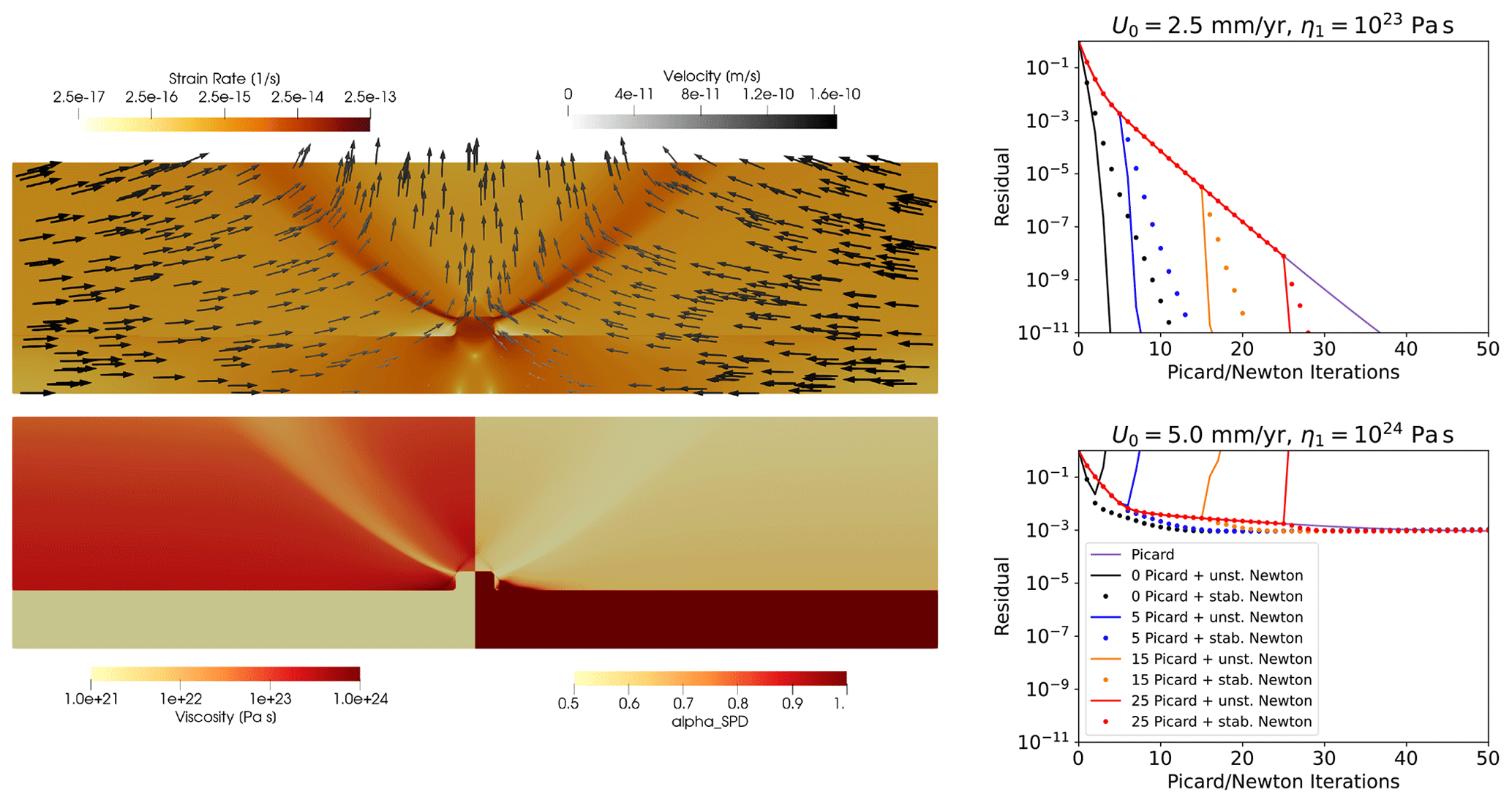
Figure 12Benchmark case of Spiegelman et al. (2016) with strain-rate- and pressure-dependent Drucker–Prager rheology. Solution fields, including velocity, strain rate, viscosity and αSPD (see Eq. 43), are shown for the case with inflow velocity U0=5 mm yr−1, η1=1024 Pa s and a friction angle of in the left panel. The top-right and bottom-right panels show convergence of the residual in the Picard and Newton solvers applied to the U0=2.5 mm yr−1, η1=1023 Pa s case and the U0=5 mm yr−1, η1=1024 Pa s case respectively. Both cases are run with a number of initial Picard iterations, as indicated in the legend, before switching to either the full unmodified Newton method (solid lines) or the stabilised method with modifications as proposed in Fraters et al. (2019) (dots). In the former case, the unmodified Newton method clearly performs best, with the stabilised method showing some degradation towards the Picard method (purple line). In the latter case, the unmodified Newton method fails to converge, whereas the stabilised method continues to converge slowly but not much faster than the Picard method, before stalling altogether. These results are generally consistent with those in Fraters et al. (2019).
To support these statements and further demonstrate the potential of the framework in exploring challenging non-linear problems, we briefly consider the non-linear benchmark case of Spiegelman et al. (2016), with a strain-rate- and pressure-dependent Drucker–Prager rheology. In Fraters et al. (2019), a number of solution strategies are explored for this case (amongst others), with the study advocating the use of two modifications to the Jacobian: (i) adding an additional term to Eq. (32) that is the transpose of the second term, thus restoring the symmetry of K, and (ii) scaling those terms associated with by a spatially varying αSPD, calculated at the Gauss points according to
where and . This rescaling acts as a stabilisation, ensuring that K remains positive definite. It should be noted that the pressure dependence of the Drucker–Prager rheology also leads to additional terms in the top-right block of the Stokes Jacobian matrix, in addition to G in Eq. (28), making the overall system asymmetric regardless.
In traditional codes, the implementation of such additional terms in the Jacobian and the proposed modifications (stabilisation) require significant development. Analytical expressions for and must be derived for each specific rheological relationship analysed (as is done in the appendices of Fraters et al., 2019), and the assembly of any additional terms may require a significant overhaul of existing code and data structures as, for example, sparsity structures may change. In Firedrake, the full Jacobian is derived symbolically and the code for its assembly generated automatically, making the entire process automatic, even for highly complex rheologies. We were able to implement the Jacobian modifications proposed in Fraters et al. (2019) in only seven lines of Python code (the full Python script for this case is available in the repository accompanying this paper) and, as illustrated in Fig. 12, we obtain similar results. As indicated in Fraters et al. (2019), the convergence of the problem gets more challenging with increased resolution, and although a reasonably converged result can be obtained for the case shown in Fig. 12 at a resolution of 1024×512, this is insufficient to resolve the details of the unstructured mesh domain used in Spiegelman et al. (2016), who reported non-convergence for this case. Firedrake's ability to choose from a large variety of discretisation types, including unstructured meshes, and its flexibility to adapt and experiment with the solution strategy open up numerous avenues to further investigate the challenges in this and other highly non-linear problems.
It is important to point out that some common components of geodynamical models have not been showcased herein and, to our knowledge, have not yet been explored within the Firedrake framework. These include, for example, a free-surface boundary condition and the ability to model multiple-material flows, often implemented in geodynamical models using the particle-in-cell technique. Our goal for this paper is to provide solid foundations for future work in Firedrake that we, and others in the geodynamical modelling community, can build upon. Nonetheless, we see no fundamental reason why any component of other geodynamical modelling tools cannot be incorporated within Firedrake. For example, the TerraFERMA framework of Wilson et al. (2017), which is built on FEniCS, has been able to match the free-surface benchmarks of Kramer et al. (2012) – a similar implementation would be straightforward in Firedrake. For multi-material flows, solving an advection equation, for example with a discontinuous Galerkin scheme and appropriate limiters (e.g. He et al., 2017), would be straightforward. In addition, particle-in-cell schemes have been successfully developed and tested with FEniCS (Maljaars et al., 2021), and we see no fundamental reason that such functionality cannot be incorporated within Firedrake. Finally, Firedrake's flexibility would make exploring different advection schemes straightforward, rendering it very well-suited to level-set approaches (e.g. Hillebrand et al., 2014).
We note that the automated approach underpinning Firedrake has the potential to revolutionise the use of adjoints and other inverse schemes in geodynamics. Adjoint models have made an enormous impact in fields such as meteorology and oceanography. However, despite significant progress (e.g. Bunge et al., 2003; Liu et al., 2008; Li et al., 2017; Colli et al., 2018; Ghelichkhan and Bunge, 2018; Ghelichkhan et al., 2020), their use in other scientific fields, including geodynamics, has been hampered by the practical difficulty of their derivation and implementation. In contrast to developing a model directly in Fortran or C++, high-level systems, such as Firedrake, allow the developer to express the variational problems to be solved in near-mathematical notation through the UFL. As such, these systems have a key advantage: since the mathematical structure of the problem is preserved, they are more amenable to automated analysis and manipulation, which can be exploited to automate the derivation of adjoints (e.g. Farrell et al., 2013; Mitush et al., 2019) and the generation of the low-level code for the derived models. Exploring the use of such an approach in geodynamics will be an important avenue for future research.
Finally, given the importance of reproducibility in the computational geosciences, we note that Firedrake integrates with Zenodo and GitHub to provide users with the ability to generate a set of DOIs corresponding to the exact set of Firedrake components used to conduct a particular set of simulations. In providing our input scripts and a DOI for the version of Firedrake used herein, we ensure traceable provenance of model data, in full compliance with FAIR principles.
Firedrake is a next-generation system for solving variational problems using the finite-element method (e.g. Rathgeber et al., 2016; Gibson et al., 2019). It treats finite-element problems as a composition of several abstract processes, using separate and open-source software components for each. Firedrake's overarching goal is to save users from manually writing low-level code for assembling the systems of equations that discretise their model physics. It is written completely in Python and exploits automatic code-generation techniques to apply sophisticated performance optimisations. Firedrake creates a separation of concerns between employing the finite-element method and implementing it: this is a game changer, as it opens up these problems to a new class of user and developer.
In this paper, we have confirmed Firedrake's applicability for geodynamical simulation by configuring and validating model predictions against a series of benchmark and analytical cases of systematically increasing complexity. In all cases, Firedrake has been shown to be accurate and efficient, and we have also demonstrated that it is flexible and easily extensible: by leveraging the UFL and PETSc, it can be effortlessly applied to problems involving different physical approximations (e.g. incompressible and compressible flow, isoviscous and more complex non-linear rheologies), even if they require distinct solution strategies. We have illustrated how Firedrake's built-in mesh generation utilities and extrusion functionality provide a straightforward mechanism for examining problems in different geometries (2-D and 3-D Cartesian, 2-D cylindrical and 3-D spherical shells) and how its fully programmable solver dictionary and customisable preconditioner interface, both of which are seamlessly coupled to PETSc, facilitate straightforward configuration of different solution approaches. Parallel scalability has been demonstrated on up to 12 288 compute cores. Finally, using a more representative simulation of global mantle dynamics, where the distribution of heterogeneity is governed by imposed plate motion histories (Müller et al., 2016), we have confirmed Firedrake's suitability for tackling challenges at the very forefront of geodynamical research. We note that all simulation data presented herein have traceable provenance: in providing our input scripts and a DOI for the exact set of Firedrake components employed, Firedrake facilitates transparency and reproducibility, in full compliance with FAIR principles.
Density changes across Earth's mantle result primarily from hydrostatic compression, with density increasing by ≈65 % from the surface to the core–mantle boundary (CMB) (e.g. Schubert et al., 2001). Variations in density associated with local temperature and pressure perturbations are small in comparison to the spherically averaged density. For a chemically homogeneous mantle, it is therefore appropriate to assume a linearised equation of state of the form
Here ρ, p, T, and α denote density, pressure, temperature, isothermal compressibility and the coefficient of thermal expansion respectively, whilst overbars refer to a reference state and primes to departures from it:
It is convenient to take the reference state as motionless and steady. Accordingly, for the purposes of the compressible case examined herein, we will assume that the reference state varies as a function of depth, z, only. The reference state pressure thus satisfies the hydrostatic approximation:
where g is the acceleration of gravity and is the unit vector in the direction opposite to gravity. On Earth, g is a function of position; however, for simplicity, it will be assumed constant for the compressible case examined herein. Following King et al. (2010), the reference density and reference temperature are described through an adiabatic Adams–Williamson equation of state (Birch, 1952), where
and
Here, cp and Ts represent the specific heat capacity at constant pressure and surface temperature respectively, whilst γ0 denotes the Grüneisen parameter, given by
where cv denotes the specific heat capacity at constant volume. Variables with a subscript 0 are constants, used in defining the reference state. Here, they are defined at the domain's upper surface.
Assuming a linearised equation of state (Eq. A1), the dimensionless form of the conservation of mass equation under the anelastic liquid approximation (ALA) can be expressed as (e.g. Schubert et al., 2001):
where u is the velocity. Neglecting inertial terms, the force balance equation becomes
where μ denotes the dynamic viscosity, I the identity tensor, Ra the Rayleigh number, and Di the dissipation number given by respectively
with κ denoting the thermal diffusivity, d the length scale and ΔT the temperature scale. Note that the last but one term in Eq. (A8) is expressed in terms of the temperature perturbation, T′ (sometimes called the potential temperature). Finally, in the absence of internal heating, conservation of energy is expressed as
where k is the thermal conductivity and Φ denotes viscous dissipation.
Table A1Highest-resolution results from the benchmark cases analysed herein. DOF: degrees of freedom for velocity (u), pressure (p) and temperature (T). Nu: surface Nusselt number.
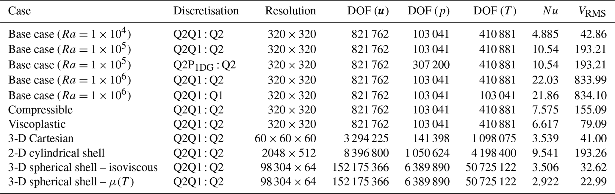
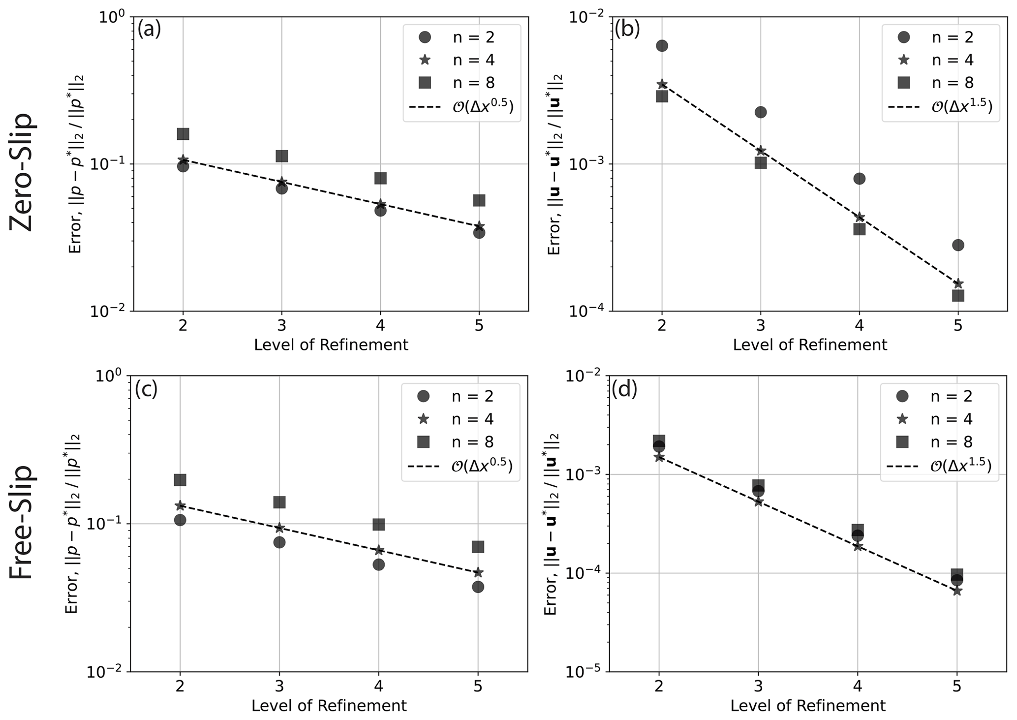
Figure A1Convergence for 2-D cylindrical shell cases with zero-slip (a–b) and free-slip (c–d) boundary conditions using a Q2Q1 finite-element pair for the Stokes system, driven by a delta-function forcing at different wave numbers, n, as indicated in the legend (see Kramer et al., 2021a, for further details). Convergence rate is indicated by dashed lines, with the order of convergence provided in the legend. For the cases plotted, the series of meshes start at refinement level 1, where the mesh consists of 1024 divisions in the tangential direction and 64 radial layers. At each subsequent level the mesh is refined by doubling resolution in both directions.
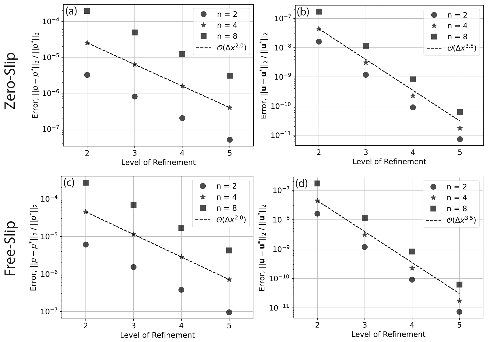
Figure A2Convergence for 2-D cylindrical shell cases with zero-slip (a–b) and free-slip (c–d) boundary conditions using a Q2P1DG finite-element pair for the Stokes system, driven by a delta-function forcing at different wave numbers, n, as indicated in the legend (see Kramer et al., 2021a, for further details). Convergence rate is indicated by dashed lines, with the order of convergence provided in the legend. For the cases plotted, the series of meshes start at refinement level 1, where the mesh consists of 1024 divisions in the tangential direction and 64 radial layers. At each subsequent level the mesh is refined by doubling resolution in both directions.
Minor adjustments to the Firedrake code base required to successfully run the cases in this paper have been merged into the open-source software associated with the Firedrake project. For the specific components of the Firedrake project used in this paper, see https://doi.org/10.5281/zenodo.6522930 (firedrake-zenodo, 2022). For the input files of all examples and benchmarks presented, see https://doi.org/10.5281/zenodo.6762752 (Davies et al., 2022).
DRD and SCK conceived this study, with all the authors having significant input on the design, development and validation of the examples and cases presented. All the authors contributed towards writing the manuscript.
The contact author has declared that neither they nor their co-authors have any competing interests.
Publisher's note: Copernicus Publications remains neutral with regard to jurisdictional claims in published maps and institutional affiliations.
Numerical simulations were undertaken at the NCI National Facility in Canberra, Australia, which is supported by the Australian Commonwealth Government. The authors are grateful to the entire Firedrake development team, particularly David Ham, for support and advice at various points of this research. We are also grateful to seven reviewers, including Cedric Thieulot, Marcus Mohr, Wolfgang Bangerth and Carsten Burstedde: their careful and constructive feedback helped to clarify and improve this contribution.
This research has been supported by the Australian Research Data Commons (ARDC), AuScope, Geosciences Australia and the National Computational Infrastructure (NCI) under G-Adopt platform grant PL031. It was also supported by the Australian Research Council under grant no. DP170100058.
This paper was edited by Rohitash Chandra and reviewed by Marcus Mohr, Cedric Thieulot, Wolfgang Bangerth, Carsten Burstedde, and three anonymous referees.
Ahrens, J., Geveci, B., and Law, C.: Paraview: An End-User Tool for Large Data Visualization, The Visualization Handbook, Elsevier, 717–731, https://doi.org/10.1016/B978-012387582-2/50038-1, 2005. a
Alisic, L., Gurnis, M., Stadler, G., Burstedde, C., Wilcox, L. C., and Ghattas, O.: Slab stress and strain rate as constraints on global mantle flow, Geophys. Res. Lett., 37, L22308, https://doi.org/10.1029/2010GL045312, 2010. a
Alnes, M. S., Logg, A., Olgaard, K. B., Rognes, M. E., and Wells, G. N.: Unified Form Language: A domain-specific language for weak formulations of partial differential equations, ACM T. Math. Softw., 40, 2–9, 2014. a, b, c, d, e
Amestoy, P., Duff, I. S., Koster, J., and L'Excellent, J.-Y.: A Fully Asynchronous Multifrontal Solver Using Distributed Dynamic Scheduling, SIAM J. Matrix Anal. A., 23, 15–41, 2001. a
Amestoy, P., Buttari, A., L'Excellent, J.-Y., and Mary, T.: Performance and Scalability of the Block Low-Rank Multifrontal Factorization on Multicore Architectures, ACM T. Math. Softw. 45, 2:1–2:26, 2019. a
Austermann, J., Kaye, B., Mitrovica, J., and Huybers, P.: A statistical analysis of the correlation between large igneous provinces and lower mantle seismic structure, Geophys. J. Int., 197, 1–9, https://doi.org/10.1093/gji/ggt500, 2014. a
Balay, S., Gropp, W. D., McInnes, L. C., and Smith, B. F.: Efficient management of parallelism in object-oriented numerical software libraries, in: Modern software tools for scientific computing, Birkhauser Boston Inc., 163–202, https://doi.org/10.1007/978-1-4612-1986-6_8, 1997. a, b, c, d, e, f
Balay, S., Abhyankar, S., Adams, M. F., Brown, J., Brune, P., Buschelman, K., Dalcin, L., Dener, A., Eijkhout, V., Gropp, W. D., Karpeyev, D., Kaushik, D., Knepley, M. G., May, D. A., McInnes, L. C., Mills, R. T., Munson, T., Rupp, K., Sanan, P., Smith, B. F., Zampini, S., Zhang, H., and Zhang, H.: PETSc Users Manual, Tech. Rep. ANL-95/11 – Revision 3.15, Argonne National Laboratory, https://www.mcs.anl.gov/petsc (last access: 1 May 2022), 2021a. a, b, c, d, e, f, g
Balay, S., Abhyankar, S., Adams, M. F., Brown, J., Brune, P., Buschelman, K., Dalcin, L., Dener, A., Eijkhout, V., Gropp, W. D., Karpeyev, D., Kaushik, D., Knepley, M. G., May, D. A., McInnes, L. C., Mills, R. T., Munson, T., Rupp, K., Sanan, P., Smith, B. F., Zampini, S., Zhang, H., and Zhang, H.: PETSc Web page, https://www.mcs.anl.gov/petsc (last access: 1 May 2022),, 2021b. a, b, c, d, e, f
Bangerth, W., Hartmann, R., and Kanschat, G.: deal.II – A general-purpose object-oriented finite element library, ACM T. Math. Software, 33, 42-es, https://doi.org/10.1145/1268776.1268779, 2007. a
Bangerth, W., Dannberg, J., Gassmoeller, R., and Heister, T.: ASPECT v2.2.0, Zenodo [code], https://doi.org/10.5281/zenodo.3924604, 2020. a, b
Baumgardner, J. R.: Three-dimensional treatment of convective flow in the Earth's mantle, J. Stat. Phys., 39, 501–511, https://doi.org/10.1007/BF01008348, 1985. a, b
Bercovici, D., Schubert, G., and Glatzmaier, G. A.: 3-D spherical models of convection in the Earth's mantle, Science, 244, 950–955, 1989. a, b, c, d
Bercovici, D., Schubert, G., and Glatzmaier, G. A.: Three-dimensional convection of an infinite-Prandtl-number compressible fluid in a basally heated spherical shell, J. Fluid Mech., 239, 683–719, 1992. a
Beucher, R., Moresi, L., Giordani, J., Mansour, J., Sandiford, D., Farrington, R., Mondy, L., Mallard, C., Rey, P., Duclaux, G., Kaluza, O., Laik, A., and Morón, S.: UWGeodynamics: A teaching and research tool for numerical geodynamic modelling, J. Open Source Softw., 4, 1136, https://doi.org/10.21105/joss.01136, 2019. a
Birch, F.: Elasticity and constitution of the Earth's interior, J. Geophys. Res., 57, 227–286, 1952. a
Blankenbach, B., Busse, F., Christensen, U., Cserepes, L., Gunkel, D., Hansen, U., Harder, H., Jarvis, G., Koch, M., Marquart, G., Moore, D., Olson, P., Schmeling, H., and Schnaubelt, T.: A benchmark comparison for mantle convection codes, Geophys. J. Int., 98, 23–38, https://doi.org/10.1111/j.1365-246X.1989.tb05511.x, 1989. a, b, c, d, e, f, g, h, i, j, k
Bower, D. J., Gurnis, M., and Seton, M.: Lower mantle structure from paleogeographically constrained dynamic Earth models, Geochem. Geophy. Geosy., 14, 44–63, https://doi.org/10.1029/2012GC004267, 2013. a, b, c
Bunge, H., Richards, M. A., and Baumgardner, J. R.: Mantle circulation models with sequential data-assimilation: inferring present-day mantle structure from plate motion histories, Philos. T. R. Soc. Lond. A, 360, 2545–2567, https://doi.org/10.1098/rsta.2002.1080, 2002. a, b
Bunge, H.-P., Richards, M. A., and Baumgardner, J. R.: The effect of depth–dependent viscosity on the planform of mantle convection, Nature, 279, 436–438, https://doi.org/10.1038/379436a0, 1996. a
Bunge, H.-P., Richards, M. A., and Baumgardner, J. R.: A sensitivity study of 3-D-spherical mantle convection at 108 Rayleigh number: effects of depth-dependent viscosity, heating mode and an endothermic phase change, J. Geophys. Res., 102, 11991–12007, https://doi.org/10.1029/96JB03806, 1997. a, b
Bunge, H.-P., Hagelberg, C. R., and Travis, B. J.: Mantle circulation models with variational data assimilation: inferring past mantle flow and structure from plate motion histories and seismic tomography, Geophys. J. Int., 152, 280–301, https://doi.org/10.1046/j.1365-246X.2003.01823.x, 2003. a
Burstedde, C., Wilcox, L. C., and Ghattas, O.: p4est: Scalable
Algorithms for Parallel Adaptive Mesh Refinement on Forests of Octrees, SIAM
J. Sci. Comput., 33, 1103–1133, https://doi.org/10.1137/100791634,
2011. a
Burstedde, C., Stadler, G., Alisic, L., Wilcox, L. C., Tan, E., Gurnis, M., and Ghattas, O.: Large-scale adaptive mantle convection simulation, Geophys. J. Int., 192, 889–906, https://doi.org/10.1093/gji/ggs070, 2013. a, b
Busse, F. H., Christensen, U., Clever, R., Cserepes, L., Gable, C., Giannandrea, E., Guillou, L., Houseman, G., Nataf, H. C., Ogawa, M., Parmentier, M., Sotin, C., and Travis, B.: 3D convection at infinite Prandtl number in Cartesian geometry - a benchmark comparison, Geophys. Astro. Fluid, 75, 39–59, https://doi.org/10.1080/03091929408203646, 1994. a, b, c, d, e, f, g, h, i, j
Choblet, G., Cadek, O., Couturier, F., and Dumoulin, C.: OEDIPUS: a new tool to study the dynamics of planetary interiors, Geophys. J. Int., 170, 9–30, https://doi.org/10.1111/j.1365-246X.2007.03419.x, 2007. a, b
Cockburn, B. and Shi, K.: Devising HDG methods for Stokes flow: An overview, Comput. Fluids, 98, 221–229, https://doi.org/10.1016/j.compfluid.2013.11.017, 2014. a
Colli, L., Ghelichkhan, S., Bunge, H., and Oeser, J.: Retrodictions of Mid Paleogene mantle flow and dynamic topography in the Atlantic region from compressible high resolution adjoint mantle convection models: Sensitivity to deep mantle viscosity and tomographic input model, Gondwana Res., 53, 252–272, https://doi.org/10.1029/2018GL077338, 2018. a
Dalcin, L., Kler, P. A., Paz, R. R., and Cosimo, A.: Parallel Distributed Computing using Python, Adv. Water Res., 34, 10.1016/j.advwatres.2011.04.013, 2011. a
Davies, D. R. and Davies, J. H.: Thermally–driven mantle plumes reconcile multiple hotspot observations, Earth Planet. Sc. Lett., 278, 50–54, https://doi.org/10.1016/j.epsl.2008.11.027, 2009. a
Davies, D. R., Wilson, C. R., and Kramer, S. C.: Fluidity: a fully unstructured anisotropic adaptive mesh computational modeling framework for geodynamics, Geochem. Geophy. Geosy., 120, Q06001, https://doi.org/10.1029/2011GC003551, 2011. a, b, c
Davies, D. R., Goes, S., Davies, J. H., Schuberth, B. S. A., Bunge, H., and Ritsema, J.: Reconciling dynamic and seismic models of Earth's lower mantle: the dominant role of thermal heterogeneity, Earth Planet. Sc. Lett., 353–354, 253–269, https://doi.org/10.1016/j.epsl.2012.08.016, 2012. a, b, c, d
Davies, D. R., Davies, J. H., Bollada, P. C., Hassan, O., Morgan, K., and Nithiarasu, P.: A hierarchical mesh refinement technique for global 3-D spherical mantle convection modelling, Geosci. Model Dev., 6, 1095–1107, https://doi.org/10.5194/gmd-6-1095-2013, 2013. a, b, c, d
Davies, D. R., Goes, S., and Lau, H. C. P.: Thermally Dominated Deep Mantle LLSVPs: A Review, in: The Earth's Heterogeneous Mantle, edited by: Khan, A. and Deschamps, F., Springer International Publishing, 441–477, https://doi.org/10.1007/978-3-319-15627-9_14, 2015a. a, b
Davies, D. R., Goes, S., and Sambridge, M.: On the relationship between volcanic hotspot locations, the reconstructed eruption sites of large igneous provinces and deep mantle seismic structure, Earth Planet. Sc. Lett., 411, 121–130, https://doi.org/10.1016/j.epsl.2014.11.052, 2015b. a
Davies, D. R., Le Voci, G., Goes, S., Kramer, S. C., and Wilson, C. R.: The mantle wedge's transient 3-D flow regime and thermal structure, Geochem. Geophy. Geosy., 17, 78–100, https://doi.org/10.1002/2015GC006125, 2016. a
Davies, D. R., Kramer, S., Ghelichkhan, S., and Gibson, A.: g-adopt/g-adopt: v1.2.0 (v1.2.0), Zenodo [code], https://doi.org/10.5281/zenodo.6762752, 2022. a
Davies, G. F.: Dynamic Earth: plates, plumes and mantle convection, Cambridge University Press, https://doi.org/10.1017/CBO9780511605802, 1999. a
Donea, J. and Huerta, A.: Finite element methods for flow problems, John Wiley & Sons, Ltd, https://doi.org/10.1002/0470013826, 2003. a
Elman, H. C., Silvester, D. J., and Wathen, A. J.: Finite elements and fast iterative solvers: with applications in incompressible fluid dynamics, Oxford University Press, https://doi.org/10.1093/acprof:oso/9780199678792.001.0001, 2005. a
Farrell, P. E., Ham, D. A., Funke, S. W., and Rognes, M. E.: Automated derivation of the adjoint of high-level transient finite element programs, SIAM J. Sci. Comput., 35, C369–C393, 2013. a
firedrake-zenodo: Software used in “Towards Automatic Finite Element Methods for Geodynamics via Firedrake” (Firedrake_20220506.0), Zenodo [code], https://doi.org/10.5281/zenodo.6522930, 2022. a
Flament, N., Bodur, Ö. F., Williams, S. E., and Merdith, A. S.: Assembly of the basal mantle structure beneath Africa, Nature, 603, 846–851, 2022. a
Fraters, M. R., Bangerth, W., Thieulot, C., Glerum, A., and Spakman, W.: Efficient and practical Newton solvers for non-linear Stokes systems in geodynamic problems, Geophys. J. Int., 218, 873–894, 2019. a, b, c, d, e, f
French, S. W. and Romanowicz, B.: Broad plumes rooted at the base of the Earth's mantle beneath major hotspots, Nature, 525, 95–99, https://doi.org/10.1038/nature14876, 2015. a
Garel, F., Goes, S., Davies, D. R., Davies, J. H., Kramer, S. C., and Wilson, C. R.: Interaction of subducted slabs with the mantle transition-zone: A regime diagram from 2-D thermo-mechanical models with a mobile trench and an overriding plate, Geochem. Geophy. Geosy., 15, 1739–1765, https://doi.org/10.1002/2014GC005257, 2014. a
Gassmoller, R., Dannberg, J., Bangerth, W., Heister, T., and Myhill, R.: On formulations of compressible mantle convection, Geophys. J. Int., 221, 1264–1280, https://doi.org/10.1093/gji/ggaa078, 2020. a
Ghelichkhan, S. and Bunge, H.: The adjoint equations for thermochemical compressible mantle convection: derivation and verification by twin experiments, Proc. Roy. Soc. A, 474, 20180329, https://doi.org/10.1098/rspa.2018.0329, 2018. a
Ghelichkhan, S., Murbock, M., Colli, L., Pail, R., and Bunge, H.: On the observability of epeirogenic movement in current and future gravity missions, Gondwana Res., 53, 273–284, https://doi.org/10.1016/j.gr.2017.04.016, 2018. a
Ghelichkhan, S., Bunge, H., and Oeser, J.: Global mantle flow retrodictions for the early Cenozoic using an adjoint method: evolving dynamic topographies, deep mantle structures, flow trajectories and sublithospheric stresses, Geophys. J. Int., 226, 1432–1460, https://doi.org/10.1093/gji/ggab108, 2020. a
Gibson, T. H., McRae, A. T. T., Cotter, C. J., Mitchell, L., and Ham, D. A.: Compatible Finite Element Methods for Geophysical Flows: Automation and Implementation using Firedrake, Springer International Publishing, https://doi.org/10.1007/978-3-030-23957-2, 2019. a, b, c, d
Glatzmaier, G. A.: Numerical simulations of mantle convection-time dependent, 3-dimensional, compressible, spherical-shell, Geophys. Astro. Fluid, 43, 223–264, 1988. a
Gurnis, M., Yang, T., Cannon, J., Turner, M., Williams, S., Flament, N., and Müller, R. D.: Global tectonic reconstructions with continuously deforming and evolving rigid plates, Comput. Geosci., 116, 32–41, https://doi.org/10.1016/j.cageo.2018.04.007, 2012. a
Ham, D. A., Farrell, P. E., Gorman, G. J., Maddison, J. R., Wilson, C. R., Kramer, S. C., Shipton, J., Collins, G. S., Cotter, C. J., and Piggott, M. D.: Spud 1.0: generalising and automating the user interfaces of scientific computer models, Geosci. Model Dev., 2, 33–42, https://doi.org/10.5194/gmd-2-33-2009, 2009. a
Hassan, R., Flament, N., Gurnis, M., Bowe, D. J., and Müller, R. D.: Provenance of plumes in global convection models, Geochem. Geophy. Geosy., 16, 1465–1489, https://doi.org/10.1002/2015GC005751, 2015. a
He, Y., Puckett, E. G., and Billen, M. I.: A Discontinuous Galerkin method with a bound preserving limiter for the advection of non-diffusive fields in solid Earth geodynamics, Phys. Earth Planet. In., 263, 23–37, 2017. a, b
Heister, T., Dannberg, J., Gassmoller, R., and Bangerth, W.: High accuracy mantle convection simulation through modern numerical methods – II: Realistic models and problems, Geophys. J. Int., 210, 833–851, https://doi.org/10.1093/gji/ggx195, 2017. a
Heroux, M. A., Bartlett, R. A., Howle, V. E., Hoekstra, R. J., Hu, J. J., Kolda, T. G., Lehoucq, R. B., Long, K. R., Pawlowski, R. P., Phipps, E. T., Salinger, A. G., Thornquist, H. K., Tuminaro, R. S., Willenbring, J. M., Williams, A., and Stanlet, K. S.: An overview of the Trilinos project, ACM T. Math. Software, 31, 397–423, https://doi.org/10.1145/1089014.1089021, 2005. a
Hillebrand, B., Thieulot, C., Geenen, T., van den Berg, A. P., and Spakman, W.: Using the level set method in geodynamical modeling of multi-material flows and Earth's free surface, Solid Earth, 5, 1087–1098, https://doi.org/10.5194/se-5-1087-2014, 2014. a
Hillewaert, K.: Development of the discontinuous Galerkin method for high-resolution, large scale CFD and acoustics in industrial geometries, PhD Thesis, Université de Louvain, 2013. a
Homolya, M., Mitchell, L., Luporini, F., and Ham, D.: Tsfc: a structure-preserving form compiler, SIAM J. Sci. Comput., 40, 401–428, https://doi.org/10.1137/17M1130642, 2018. a, b, c
Hunt, S. A., Davies, D. R., Walker, A. M., McCormack, R. J., Wills, A. S., Dobson, D. P., and Li, L.: On the increase in thermal diffusivity caused by the perovskite to post-perovskite phase transition and its implications for mantle dynamics, Earth Planet. Sc. Lett., 319, 96–103, https://doi.org/10.1016/j.epsl.2011.12.009, 2012. a
Jadamec, M. A.: Insights on slab-driven mantle flow from advances in three-dimensional modelling, J. Geodynam., 100, 51–70, 2016. a
Jadamec, M. A. and Billen, M. I.: Reconciling surface plate motions with rapid three-dimensional mantle flow around a slab edge, Nature, 465, 338–341, 2010. a
Jarvis, G. T.: Effects of curvature on two–dimensional models of mantle convection: cylindrical polar coordinates, J. Geophys. Res., 98, 4477–4485, 1993. a
Jarvis, G. T. and McKenzie, D. P.: Convection in a compressible fluid with infinite Prandtl number, J. Fluid Mech., 96, 515–583, https://doi.org/10.1017/S002211208000225X, 1980. a
Katz, R. F. and Weatherley, S. M.: Consequences of mantle heterogeneity for melt extraction at mid-ocean ridges, Earth Planet. Sc. Lett., 335, 226–237, https://doi.org/10.1016/j.epsl.2012.04.042, 2012. a
King, S. D., Lee, C., van Keken, P. E., Leng, W., Zhong, S., Tan, E., Tosi, N., and Kameyama, M. C.: A community benchmark for 2-D Cartesian compressible convection in Earth's mantle, Geophys. J. Int., 179, 1–11, 2010. a, b, c, d, e, f, g, h, i, j
Kirby, R. C.: Algorithm 839: FIAT, a new paradigm for computing finite element basis functions, ACM T. Math. Software, 30, 502–516, 2004. a
Kirby, R. C. and Mitchell, L.: Solver Composition Across the PDE/Linear Algebra Barrier, SIAM J. Sci. Comput., 40, 76–98, https://doi.org/10.1137/17M1133208, 2018. a, b
Kirby, R. C. and Mitchell, L.: Code generation for generally mapped finite elements, ACM T. Math. Software, 45, 1–23, 2019. a, b, c
Knepley, M. G. and Karpeev, D. A.: Mesh Algorithms for PDE with Sieve I: Mesh Distribution, Sci. Program., 17, 215–230, 2009. a
Koelemeijer, P. J., Schuberth, B. S. A., Davies, D. R., Deuss, A., and Ritsema, J.: Constraints on the presence of post-perovskite in Earth's lowermost mantle from tomographic-geodynamic model comparisons, Geophys. J. Int., 494, 226–238, 2018. a
Kramer, S. C., Cotter, C. J., and Pain, C. C.: Solving the Poisson equation on small aspect ratio domains using unstructured meshes, Ocean Model., 35, 253–263, 2010. a
Kramer, S. C., Wilson, C. R., and Davies, D. R.: An implicit free-surface algorithm for geodynamical simulations, Phys. Earth Planet. In., 194, 25–37, https://doi.org/10.1016/j.pepi.2012.01.001, 2012. a, b
Kramer, S. C., Davies, D. R., and Wilson, C. R.: Analytical solutions for mantle flow in cylindrical and spherical shells, Geosci. Model Dev., 14, 1899–1919, https://doi.org/10.5194/gmd-14-1899-2021, 2021a. a, b, c, d, e, f, g, h, i, j, k, l, m
Kramer, S. C., Wilson, C., Davies, D. R., Mathews, C., Gibson, A., Dubernay, T., Greaves, T., Candy, A., Cotter, C. J., Percival, J., Mouradian, S., Bhutani, G., Avdis, A., Gorman, G., Piggott, M., and Ham, D.: FluidityProject/fluidity: Zenodo release, Zenodo [code], https://doi.org/10.5281/zenodo.3924604, 2021b. a
Kronbichler, M., Heister, T., and Bangerth, W.: High accuracy mantle convection simulation through modern numerical methods, Geophys. J. Int., 191, 12–29, https://doi.org/10.1111/j.1365-246X.2012.05609.x, 2012. a, b
Kärnä, T., Kramer, S. C., Mitchell, L., Ham, D. A., Piggott, M. D., and Baptista, A. M.: Thetis coastal ocean model: discontinuous Galerkin discretization for the three-dimensional hydrostatic equations, Geosci. Model Dev., 11, 4359–4382, https://doi.org/10.5194/gmd-11-4359-2018, 2018. a
Lange, M., Mitchell, L., Knepley, M. G., and Gorman, G. J.: Efficient mesh management in Firedrake using PETSc-DMPlex, SIAM J. Sci. Comput., 38, S143–S155, https://doi.org/10.1137/15M1026092, 2016. a
Le Voci, G., Davies, D. R., Goes, S., Kramer, S. C., and Wilson, C. R.: A systematic 2-D investigation into the mantle wedge's transient flow regime and thermal structure: complexities arising from a hydrated rheology and thermal buoyancy, Geochem. Geophy. Geosy., 15, 28–51, https://doi.org/10.1002/2013GC005022, 2014. a
Leng, W. and Zhong, S.: Viscous heating, adiabatic heating and energetic consistency in compressible mantle convection, Geophys. J. Int., 173, 693–702, 2008. a
Li, D., Gurnis, M., and Stadler, G.: Towards adjoint-based inversion of time-dependent mantle convection with nonlinear viscosity, Geophys. J. Int., 209, 86–105, https://doi.org/10.1093/gji/ggw493, 2017. a
Liu, L., Spasojevic, S., and Gurnis, M.: Reconstructing Farallon Plate Subduction Beneath North America Back to the Late Cretaceous, Science, 322, 934–938, https://doi.org/10.1126/science.1162921, 2008. a
Liu, S. and King, S. D.: A benchmark study of incompressible Stokes flow in a 3-D spherical shell using ASPECT, Geophys. J. Int., 217, 650–667, 2019. a, b
Logg, A., Mardal, K.-A., and Wells, G.: Automated Solution of Differential Equations by the Finite Element Method: The FEniCS Book, Lecture Notes in Computational Science and Engineering vol. 84, Springer, Berlin, https://doi.org/10.1007/978-3-642-23099-8, 2012. a, b, c, d, e
Maljaars, J. M., Richardson, C. N., and Sime, N.: LEoPart: A particle library for FEniCS, Comp. Math. Appl., 81, 289–315, 2021. a
Markall, G. R., Rathgeber, F., Mitchell, L., Loriant, N., Bertolli, C., Ham, D. A., and Kelly, P. H. J.: Performance-Portable Finite Element Assembly Using PyOP2 and FEniCS, in: 28th International Supercomputing Conference, ISC, Proceedings, edited by: Kunkel, J. M., Ludwig, T., and Meuer, H. W., vol. 7905 of Lecture Notes in Computer Science, Springer, 279–289, https://doi.org/10.1007/978-3-642-38750-0_21, 2013. a
May, D. and Moresi, L.: Preconditioned iterative methods for Stokes flow problems arising in computational geodynamics, Phys. Earth Planet. In., 171, 33–47, https://doi.org/10.1016/j.pepi.2008.07.036, 2008. a, b, c, d, e
McKenzie, D.: Speculations on consequences and causes of plate motions, Geophys. J. Roy. Astr. S., 18, 1–18, 1969. a
McKenzie, D. P., Roberts, J. M., and Weiss, N. O.: Numerical models of convection in the Earth's mantle, Tectonophys., 19, 89–103, https://doi.org/10.1016/0040-1951(73)90034-6, 1973. a, b
Minear, J. and Toksoz, M.: Thermal regime of a downgoing slab and new global tectonics, J. Geophys. Res., 75, 1397–1419, 1970. a
Mitush, S. K., Funke, S. W., and Dokken, J. S.: dolfin-adjoint 2018.1: automated adjoints for FEniCS and Firedrake, J. Open Source Softw., 4, 1292, https://doi.org/10.21105/joss.01292, 2019. a
Moresi, L., Dufour, F., and Muhlhaus, H.: Mantle convection modeling with viscoelastic/brittle lithosphere: Numerical methodology and plate tectonic modeling, Pure Appl. Geophys., 159, 2335–2356, 2002. a
Moresi, L., Quenette, S., Lemiale, V., Meriaux, C., Appelbe, B., and Muhlhaus, H.-B.: Computational approaches to studying non-linear dynamics of the crust and mantle, Phys. Earth Planet. In., 163, 69–82, https://doi.org/10.1016/j.pepi.2007.06.009, 2007. a
Moresi, L. N. and Solomatov, V. S.: Numerical investigations of 2D convection with extremely large viscosity variations, Phys. Fluid, 7, 2154–2162, https://doi.org/10.1063/1.868465, 1995. a
Müller, R. D., Seton, M., Zahirovic, S., Williams, S. E., Matthews, K. J., Wright, N. M., Shephard, G. E., Maloney, K. T., Barnett-Moore, N., Hosseinpour, M., Bower, D. J., and Cannon, J.: Ocean Basin Evolution and Global-Scale Plate Reorganization Events Since Pangea Breakup, Annu. Rev. Earth Pl. Sc., 44, 107–138, https://doi.org/10.1146/annurev-earth-060115-012211, 2016. a, b, c, d
Müller, R. D., Cannon, J., Qin, X., Watson, R. J., Gurnis, M., Williams, S., Pfaffelmoser, T., Seton, M., Russell, S. H. J., and Zahirovic, S.: GPlates: Building a Virtual Earth Through Deep Time, Geochem. Geophy. Geosy., 19, 2243–2261, https://doi.org/10.1029/2018GC007584, 2018. a
Nakagawa, T., Tackley, P. J., Deschamps, F., and Connolly, J. A. D.: Incorporating self–consistently calculated mineral physics into thermo–chemical mantle convection simulations in a 3-D spherical shell and its influence on seismic anomalies in Earth's mantle, Geochem. Geophy. Geosy., 10, Q3304, https://doi.org/10.1029/2008GC002280, 2009. a
Nerlich, R., Colli, L., Ghelichkhan, S., Schuberth, B., and Bunge, H.-P.: Constraining entral Neo-Tethys Ocean reconstructions with mantle convection models, Geophys. Res. Lett., 43, 9595–9603, https://doi.org/10.1002/2016GL070524, 2016. a
Nitsche, J.: Über ein Variationsprinzip zur Lösung von Dirichlet-Problemen bei Verwendung von Teilräumen, die keinen Randbedingungen unterworfen sind, in: Abhandlungen aus dem mathematischen Seminar der Universität Hamburg, Springer, vol. 36, 9–15, https://doi.org/10.1007/BF02995904, 1971. a
Quenette, S., Moresi, L., Appelbe, B. F., and Sunter, P. D.: Explaining StGermain: an aspect oriented environment for building extensible computational mechanics modeling software, IEEE International Parallel and Distributed Processing Symposium, IEEE New York, 210 pp., https://doi.org/10.1109/IPDPS.2007.370400, 2007. a
Ratcliff, J. T., Schubert, G., and Zebib, A.: Steady tetrahedral and cubic patterns of spherical shell convection with temperature-dependent viscosity, J. Geophys. Res., 101, 25473–25484, https://doi.org/10.1029/96JB02097, 1996. a, b, c
Rathgeber, F., Markall, G. R., Mitchell, L., Loriant, N., Ham, D. A., Bertolli, C., and Kelly, P. H. J.: PyOP2: A High-Level Framework for Performance-Portable Simulations on Unstructured Meshes, in: High Performance Computing, Networking Storage and Analysis, SC Companion, IEEE Computer Society, Los Alamitos, CA, USA, 1116–1123, https://doi.org/10.1109/SC.Companion.2012.134, 2012. a
Rathgeber, F., Ham, D. A., Mitchell, L., Lange, M., Luporini, F., Mcrae, A. T. T., Bercea, G.-T., Markall, G. R., and Kelly, P. H. J.: Firedrake: Automating the Finite Element Method by Composing Abstractions, ACM T. Math. Softw., 43, 1–27, https://doi.org/10.1145/2998441, 2016. a, b, c, d, e, f, g, h, i, j
Ritsema, J., Deuss, A., van Heijst, H. J., and Woodhouse, J. H.: S40RTS: a degree-40 shear-velocity model for the mantle from new Rayleigh wave dispersion, teleseismic traveltime and normal-mode splitting function measurements, Geophys. J. Int., 184, 1223–1236, https://doi.org/10.1111/j.1365-246X.2010.04884.x, 2011. a
Rubey, M., Brune, S., Heine, C., Davies, D. R., Williams, S. E., and Müller, R. D.: Global patterns in Earth's dynamic topography since the Jurassic: the role of subducted slabs, Solid Earth, 8, 899–919, https://doi.org/10.5194/se-8-899-2017, 2017. a
Saad, Y.: A flexible inner-outer preconditioned GMRES algorithm, SIAM J. Sci. Comput., 14, 461–469, 1993. a
Schubert, G., Turcotte, D. L., and Olson, P.: Mantle convection in the Earth and planets, Cambridge University Press, https://doi.org/10.1017/CBO9780511612879, 2001. a, b, c, d, e
Schuberth, B. S. A., H.-P. Bunge, Steinle-Neumann, G., Moder, C., and Oeser, J.: Thermal versus elastic heterogeneity in high-resolution mantle circulation models with pyrolite composition: high plume excess temperatures in the lowermost mantle, Geochem. Geophy. Geosy., 10, Q01W01, https://doi.org/10.1029/2008GC002235, 2009. a
Shahbazi, K.: An explicit expression for the penalty parameter of the interior penalty method, J. Comput. Phys., 205, 401–407, 2005. a
Shapero, D. R., Badgeley, J. A., Hoffman, A. O., and Joughin, I. R.: icepack: a new glacier flow modeling package in Python, version 1.0, Geosci. Model Dev., 14, 4593–4616, https://doi.org/10.5194/gmd-14-4593-2021, 2021. a
Shih, Y., Stadler, G., and Wechsung, F.: Robust multigrid techniques for augmented Lagrangian preconditioning of incompressible Stokes equations with extreme viscosity variations, arXiv [preprint], arXiv:2107.00820, 2021. a
Shipton, J., Gibson, T., and Cotter, C.: Higher-order compatible finite element schemes for the nonlinear rotating shallow water equations on the sphere, J. Comput. Phys., 375, 1121–1137, https://doi.org/10.1016/j.jcp.2018.08.027, 2018. a
Spiegelman, M., May, D. A., and Wilson, C. R.: On the solvability of incompressible Stokes with viscoplastic rheologies in geodynamics, Geochem. Geophy. Geosy., 17, 2213–2238, https://doi.org/10.1002/2015GC006228, 2016. a, b, c
Stadler, G., Gurnis, M., Burstedde, C., Wilcox, L. C., Alisic, L., and Ghattas, O.: The dynamics of plate tectonics and mantle flow: from local to global scales, Science, 329, 1033–1038, https://doi.org/10.1126/science.1191223, 2010. a, b
Stemmer, K., Harder, H., and Hansen, U.: A new method to simulate convection with strongly temperature- and pressure-dependent viscosity in a spherical shell: Applications to the Earth's mantle, Phys. Earth Planet. In., 157, 223–249, https://doi.org/10.1016/j.pepi.2006.04.007, 2006. a, b
Styles, E., Davies, D. R., and Goes, S.: Mapping spherical seismic into physical structure: biases from 3-D phase-transition and thermal boundary-layer heterogeneity, Geophys. J. Int., 184, 1371–1378, https://doi.org/10.1111/j.1365-246X.2010.04914.x, 2011. a
Tackley, P. J.: Effects of strongly variable viscosity on three–dimensional compressible convection in planetary mantles, J. Geophys. Res., 101, 3311–3332, https://doi.org/10.1029/95JB03211, 1996. a
Tackley, P. J.: Mantle convection and plate tectonics: towards and integrated physical and chemical theory, Science, 288, 2002–2007, 2000. a
Tackley, P. J.: Modelling compressible mantle convection with large viscosity contrasts in a three-dimensional spherical shell using the Yin-Yang grid, Phys. Earth Planet. In., 171, 7–18, https://doi.org/10.1016/j.pepi.2008.08.005, 2008. a, b, c
Tackley, P. J. and Xie, S.: The thermo-chemical structure and evolution of Earth's mantle: constraints and numerical models, Philos. T. R. Soc. Lond. A., 360, 2593–2609, 2002. a
Tackley, P. J., Stevenson, D. J., Glatzmaier, G. A., and Schubert, G.: Effects of an endothermic phase transition at 670 km depth in a spherical model of convection in the Earth's mantle, Nature, 361, 699–704, https://doi.org/10.1038/361699a0, 1993. a
Thieulot, C. and Bangerth, W.: On the choice of finite element for applications in geodynamics, Solid Earth, 13, 229–249, https://doi.org/10.5194/se-13-229-2022, 2022. a, b
Torrance, K. E. and Turcotte, D. L.: Thermal convection with large viscosity variations, J. Fluid Mech., 47, 113–125, 1971. a
Tosi, N., Stein, C., Noack, L., Hüttig, C., Maierová, P., Samuel, H., Davies, D. R., Wilson, C. R., Kramer, S. C., Thieulot, C., Glerum, A., Fraters, M., Spakman, W., Rozel, A., and Tackley, P. J.: A community benchmark for viscoplastic thermal convection in a 2-D square box, Geochem. Geophy. Geosy., 16, 2175–2196, https://doi.org/10.1002/2015GC005807, 2015. a, b, c, d, e, f, g, h, i, j, k
Trilinos Project Team, T.: The Trilinos Project Website, https://trilinos.github.io, last access: 22 May 2020. a
Trompert, R. and Hansen, U.: Mantle convection simulations with rheologies that generate plate-like behaviour, Nature, 395, 686–689, 1998. a
van Keken, P.: Evolution of starting mantle plumes: a comparison between numerical and laboratory models, Earth Planet. Sc. Lett., 148, 1–11, https://doi.org/10.1016/S0012-821X(97)00042-3, 1997. a
van Keken, P. E. and Ballentine, C. J.: Whole–mantle versus layered mantle convection and the role of a high–viscosity lower mantle in terrestrial volatile evolution, Earth Planet. Sc. Lett., 156, 19–32, 1998. a
Vanek, P., Mandel, J., and Brezina, M.: Algebraic multigrid by smoothed aggregation for second and fourth order elliptic problems, Computing, 56, 179–196, https://doi.org/10.1007/BF02238511, 1996. a
Vynnytska, L., Rognes, M. E., and Clark, S. R.: Benchmarking FEniCS for mantle convection simulations, Compu. Geosci., 50, 95–105, https://doi.org/10.1016/j.cageo.2012.05.012, 2013. a, b
Wilson, C. R., Spiegelman, M., van Keken, P. E., and R., H. B.: Fluid flow in subduction zones: The role of solid rheology and compaction pressure, Earth Planet. Sc. Lett., 401, 261–274, https://doi.org/10.1016/j.epsl.2014.05.052, 2014. a
Wilson, C. R., Spiegelman, M., and van Keken, P. E.: TerraFERMA: The Transparent Finite Element Rapid Model Assembler for multiphysics problems in Earth sciences, Geochem. Geophy. Geosy., 18, 769–810, https://doi.org/10.1002/2016GC006702, 2017. a, b, c, d, e, f, g
Wolstencroft, M., Davies, J. H., and Davies, D. R.: Nusselt-Rayleigh number scaling for spherical shell Earth mantle simulation up to a Rayleigh number of 109, Phys. Earth Planet. In., 176, 132–141, https://doi.org/10.1016/j.pepi.2009.05.002, 2009. a
Yoshida, M. and Kageyama, A.: Application of the Yin-Yang grid to a thermal convection of a Boussinesq fluid with infinite Prandtl number in a three-dimensional spherical shell, Geophys. Res. Lett., 31, L12609, https://doi.org/10.1029/2004GL019970, 2004. a, b
Zhong, S., Zuber, M. T., Moresi, L., and Gurnis, M.: Role of temperature-dependent viscosity and surface plates in spherical shell models of mantle convection, J. Geophys. Res., 105, 11063–11082, https://doi.org/10.1029/2000JB900003, 2000. a
Zhong, S., McNamara, A., Tan, E., Moresi, L., and Gurnis, M.: A benchmark study on mantle convection in a 3-D spherical shell using CitcomS, Geochem. Geophy. Geosy., 9, Q10017, https://doi.org/10.1029/2008GC002048, 2008. a, b, c, d, e, f, g, h, i, j, k, l, m
Zienkiewicz, O. C., Taylor, R. L., and Zhu, J. Z.: The finite element method: its basis and fundamentals, Elsevier, ISBN 9780080472775, 2005. a
- Abstract
- Introduction
- Firedrake
- Governing equations
- Finite-element discretisation and solution strategy
- Examples: benchmark cases and validation
- Parallel scaling
- Application in 3-D spherical shell geometry: global mantle convection
- Discussion
- Conclusions
- Appendix A: Governing equations under the anelastic liquid approximation
- Code and data availability
- Author contributions
- Competing interests
- Disclaimer
- Acknowledgements
- Financial support
- Review statement
- References