The GPU version of LASG/IAP Climate System Ocean Model version 3 (LICOM3) under the heterogeneous-compute interface for portability (HIP) framework and its large-scale application

A high-resolution ($\mathrm{1}/\mathrm{20}{}^{\circ }$) global ocean general circulation model with graphics processing unit (GPU) code implementations is developed based on the LASG/IAP Climate System Ocean Model version 3 (LICOM3) under a heterogeneous-compute interface for portability (HIP) framework. The dynamic core and physics package of LICOM3 are both ported to the GPU, and three-dimensional parallelization (also partitioned in the vertical direction) is applied. The HIP version of LICOM3 (LICOM3-HIP) is 42 times faster than the same number of CPU cores when 384 AMD GPUs and CPU cores are used. LICOM3-HIP has excellent scalability; it can still obtain a speedup of more than 4 on 9216 GPUs compared to 384 GPUs. In this phase, we successfully performed a test of $\mathrm{1}/\mathrm{20}{}^{\circ }$ LICOM3-HIP using 6550 nodes and 26 200 GPUs, and on a large scale, the model's speed was increased to approximately 2.72 simulated years per day (SYPD). By putting almost all the computation processes inside GPUs, the time cost of data transfer between CPUs and GPUs was reduced, resulting in high performance. Simultaneously, a 14-year spin-up integration following phase 2 of the Ocean Model Intercomparison Project (OMIP-2) protocol of surface forcing was performed, and preliminary results were evaluated. We found that the model results had little difference from the CPU version. Further comparison with observations and lower-resolution LICOM3 results suggests that the $\mathrm{1}/\mathrm{20}{}^{\circ }$ LICOM3-HIP can reproduce the observations and produce many smaller-scale activities, such as submesoscale eddies and frontal-scale structures.

1 Introduction

Numerical models are a powerful tool for weather forecasts and climate prediction and projection. Creating high-resolution atmospheric, oceanic, and climatic models remains a significant scientific and engineering challenge because of the enormous computing, communication, and input and/or output (IO) involved. Kilometer-scale weather and climate simulation have recently started to emerge (Schär et al., 2020). Due to the considerable increase in computational cost, such models will only work with extreme-scale high-performance computers and new technologies.

Global ocean general circulation models (OGCMs) are a fundamental tool for oceanography research, ocean forecasting, and climate change research (Chassignet et al., 2019). Such model performance is determined mainly by model resolution and subgrid parameterization and surface forcing. The horizontal resolution of global OGCMs has increased to approximately 5–10 km, and these models are also called eddy-resolving models. Increasing the resolution will significantly improve the simulation of western boundary currents, mesoscale eddies, fronts and jets, and currents in narrow passages (Hewitt et al., 2017). Meanwhile, the ability of an ocean model to simulate the energy cascade (Wang et al., 2019), the air–sea interaction (Hewitt et al., 2017), and the ocean heat uptake (Griffies et al., 2015) will be improved with increasing resolution. All these factors will effectively improve ocean model performance in the simulation and prediction of ocean circulation. Additionally, the latest numerical and observational results show that much smaller eddies (submesoscale eddies with a spatial scale of approximately 5–10 km) are crucial to vertical heat transport in the upper-ocean mixed layer and significant to biological processes (Su et al., 2018). Resolving the smaller-scale processes raises a new challenge for the horizontal resolution of OGCMs, which also demands much more computing resources.

Heterogeneous computing has become a development trend of high-performance computers. In the latest TOP500 supercomputer list released in November 2020 (https://www.top500.org/lists/top500/2020/11/, last access: 17 May 2021), central processing unit (CPU) and graphics processing unit (GPU) heterogeneous machines account for 6 of the top 10. After the NVIDIA Corporation provided supercomputing techniques on GPUs, an increasing number of ocean models applied these high-performance acceleration methods to conduct weather or climate simulations. Xu et al. (2015) developed POM.gpu (GPU version of the Princeton Ocean Model), a full GPU solution based on mpiPOM (MPI version of the Princeton Ocean Model) on a cluster, and achieved a 6.8 times energy reduction. Yashiro et al. (2016) deployed the NICAM (Nonhydrostatic ICosahedral Atmospheric Model) on the TSUBAME supercomputer, and the model sustained a double-precision performance of 60 teraflops on 2560 GPUs. Yuan et al. (2020) developed a GPU version of a wave model with 2 V100 cards and obtained a speedup of 10–12 times when compared to the 36 cores of the CPU. Yang et al. (2016) implemented a fully implicit β-plane dynamic model with 488 m grid spacing on the TaihuLight system and achieved 7.95 petaflops. Fuhrer et al. (2018) reported a 2 km regional atmospheric general circulation model (AGCM) test using 4888 GPU cards and obtained a simulation performance for 0.043 simulated years per wall clock day (SYPD). S. Zhang et al. (2020) successfully ported a high-resolution (25 km atmosphere and 10 km ocean) Community Earth System Model in the TaihuLight supercomputer and obtained 1–3.4 SYPD.

Additionally, the AMD company also provides GPU solutions. In general, AMD GPUs use heterogeneous compute compiler (HCC) tools to compile codes, and they cannot use the Compute Unified Device Architecture (CUDA) development environments, which provide support for the NVIDIA GPU only. Therefore, due to the wide use and numerous CUDA learning resources, AMD developers must study two kinds of GPU programming skills. AMD's heterogeneous-compute interface for portability (HIP) is an open-source solution to address this problem. It provides a higher-level framework to contain these two types of lower-level development environments, i.e., CUDA and HCC, simultaneously. The HIP code's grammar is similar to that of the CUDA code, and with a simple conversion tool, the code can be compiled and run at CUDA and AMD architects. HCC/OpenACC (Open ACCelerators) is more convenient for AMD GPU developers than the HIP, which is popular from the coding viewpoint. Another reason is that CUDA GPUs currently have more market share. It is believed that an increasing number of codes will be ported to the HIP in the future. However, almost no ocean models use the HIP framework to date.

This study aims to develop a high-performance OGCM based on the LASG/IAP Climate System Ocean Model version 3 (LICOM3), which can be run on an AMD GPU architecture using the HIP framework. Here, we will focus on the model's best or fastest computing performance and its practical usage for research and operation purposes. Section 2 is the introduction of the LICOM3 model. Section 3 contains the main optimization of LICOM3 under HIP. Section 4 covers the performance analysis and model verification. Section 5 is a discussion, and the conclusion is presented in Sect. 6.

2 The LICOM3 model and experiments

2.1 The LICOM3 model

In this study, the targeting model is LICOM3, which was developed in the late 1980s (Zhang and Liang, 1989). Currently, LICOM3 is the ocean model for two air–sea coupled models of CMIP6 (the Coupled Model Intercomparison Project phase 6), the Flexible Global Ocean-Atmosphere-Land System model version 3 with a finite-volume atmospheric model (FGOALS-f3; He et al., 2020), and the Flexible Global Ocean-Atmosphere-Land System model version 3 with a grid-point atmospheric model (Chinese Academy of Science, CAS, FGOALS-g3; L. Li et al., 2020). LICOM version 2 (LICOM2.0, Liu et al., 2012) is also the ocean model of the CAS Earth System Model (CAS-ESM, H. Zhang et al., 2020). A future paper to fully describe the new features and baseline performances of LICOM3 is in preparation.

In recent years, the LICOM model was substantially improved based on LICOM2.0 (Liu et al., 2012). There are three main aspects. First, the coupling interface of LICOM has been upgraded. Now, the NCAR flux coupler version 7 is employed (Lin et al., 2016), in which memory use has been dramatically reduced (Craig et al., 2012). This makes the coupler suitable for application to high-resolution modeling.

Second, both orthogonal curvilinear coordinates (Murray, 1996; Madec and Imbard, 1996) and tripolar grids have been introduced in LICOM. Now, the two poles are at 60.8^∘ N, 65^∘ E and 60.8^∘ N, 115^∘ W for the 1^∘ model, at 65^∘ N, 65^∘ E and 65^∘ N, 115^∘ W for the 0.1^∘ model, and at 60.4^∘ N, 65^∘ E and 60.4^∘ N, 115^∘ W for the $\mathrm{1}/\mathrm{20}{}^{\circ }$ model of LICOM. After that, the zonal filter at high latitudes, particularly in the Northern Hemisphere, was eliminated, which significantly improved the scalability and efficiency of the parallel algorithm of the LICOM3 model. In addition, the dynamic core of the model has also been updated accordingly (Yu et al., 2018), including the application of a new advection scheme for the tracer formulation (Xiao, 2006) and the addition of a vertical viscosity for the momentum formulation (Yu et al., 2018).

Third, the physical package has been updated, including introducing an isopycnal and thickness diffusivity scheme (Ferreira et al., 2005) and vertical mixing due to internal tides breaking at the bottom (St. Laurent et al., 2002). The coefficient of both isopycnal and thickness diffusivity is set to 300 m² s⁻¹ as the depth is either within the mixed layer or the water depth is shallower than 60 m. The upper and lower boundary values of the coefficient are 2000 and 300 m² s⁻¹, respectively. Additionally, the chlorophyll-dependent solar shortwave radiation penetration scheme of Ohlmann (2003), the isopycnal mixing scheme (Redi, 1982; Gent and McWilliams, 1990), and the vertical viscosity and diffusivity schemes (Canuto et al., 2001, 2002) are employed in LICOM3.

Both the low-resolution (1^∘; Lin et al., 2020) and high-resolution ($\mathrm{1}/\mathrm{10}{}^{\circ }$; Y. Li et al., 2020) stand-alone LICOM3 versions are also involved in the Ocean Model Intercomparison Project (OMIP)-1 and OMIP-2; their outputs can be downloaded from websites. The two versions of LICOM3's performances compared with other CMIP6 ocean models are shown in Tsujino et al. (2020) and Chassignet et al. (2020). The $\mathrm{1}/\mathrm{10}{}^{\circ }$ version has also been applied to perform short-term ocean forecasts (Liu et al., 2021).

The essential task of the ocean model is to solve the approximated Navier–Stokes equations, along with the conservation equations of the temperature and salinity. Seven kernels are within the time integral loop, named “readyt”, “readyc”, “barotr”, “bclinc”, “tracer”, “icesnow”, and “convadj”, which are also the main subroutines porting from the CPU to the GPU. The first two kernels computed the terms in the barotropic and baroclinic equations of the model. The next three (barotr, bclinc, and tracer) are used to solve the barotropic, baroclinic, and temperature and/or salinity equations. The last two subroutines deal with sea ice and deep convection processes at high latitudes. All these subroutines have approximately 12 000 lines of source code, accounting for approximately 25 % of the total code and 95 % of computation.

2.2 Configurations of the models

To investigate the GPU version, we employed three configurations in the present study. They are 1^∘, 0.1^∘, and $\mathrm{1}/\mathrm{20}{}^{\circ }$. Details of these models are listed in Table 1. The number of horizontal grid points for the three configurations are 360×218, 3600×2302, and 7200×3920. The vertical levels for the low-resolution models are 30, while they are 55 for the other two high-resolution models. From 1^∘ to $\mathrm{1}/\mathrm{20}{}^{\circ }$, the computational effort increased by approximately 8000 (20³) times (considering 20 times to decrease the time step), and the vertical resolution increased from 30 to 55, in total, by approximately 15 000 times. The original CPU version of $\mathrm{1}/\mathrm{20}{}^{\circ }$ with MPI (Message Passing Interface) parallel on Tianhe-1A only reached 0.31 SYPD using 9216 CPU cores. This speed will slow down the 10-year spin-up simulation of LICOM3 to more than 1 month, which is not practical for climate research. Therefore, such simulations require extreme-scale high-performance computers by applying the GPU version.

Table 1 Configurations of the LICOM3 model used in the present study.

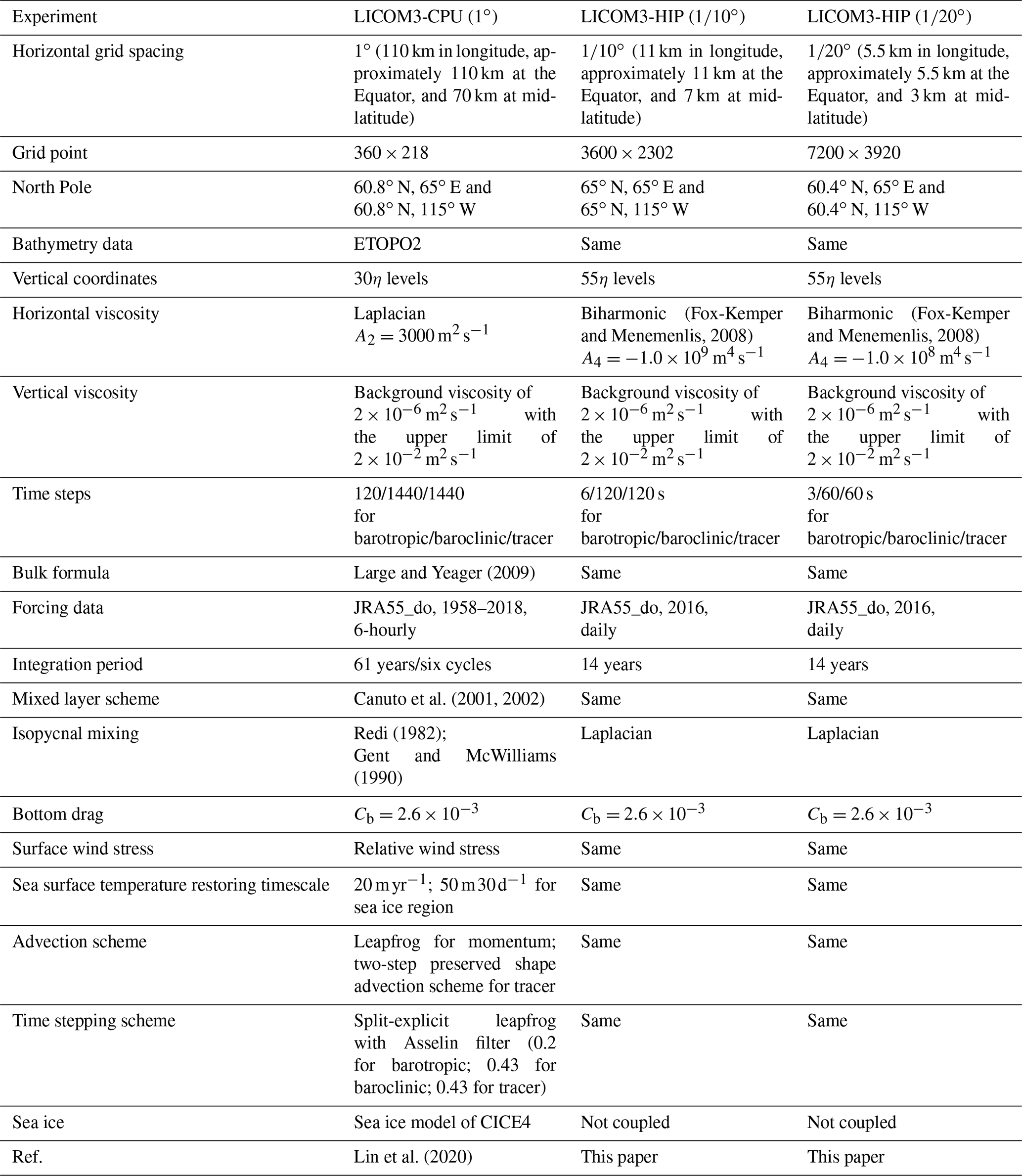
In addition to the different grid points, three main aspects are different among the three experiments, particularly between version 1^∘ and the other two versions. First, the horizontal viscosity schemes are different: using Laplacian for 1^∘ and biharmonic for $\mathrm{1}/\mathrm{10}{}^{\circ }$ and $\mathrm{1}/\mathrm{20}{}^{\circ }$. The viscosity coefficient is 1 order of magnitude smaller for the $\mathrm{1}/\mathrm{20}{}^{\circ }$ version than for the $\mathrm{1}/\mathrm{10}{}^{\circ }$ version, namely, $-\mathrm{1.0}\times {\mathrm{10}}^{\mathrm{9}}$ m⁴ s⁻¹ for $\mathrm{1}/\mathrm{10}{}^{\circ }$ vs. $-\mathrm{1.0}\times {\mathrm{10}}^{\mathrm{8}}$ m⁴ s⁻¹ for $\mathrm{1}/\mathrm{20}{}^{\circ }$. Second, although the force-including dataset (the Japanese 55-year reanalysis dataset for driving ocean–sea-ice models, JRA55-do; Tsujino et al., 2018) and the bulk formula for the three experiments are all a standard of the OMIP-2, the periods and temporal resolutions of the forcing fields are different: 6 h data from 1958 to 2018 for the 1^∘ version and daily mean data in 2016 for both the $\mathrm{1}/\mathrm{10}{}^{\circ }$ and $\mathrm{1}/\mathrm{20}{}^{\circ }$ versions. Third, version 1^∘ is coupled with a sea ice model of CICE4 (Community Ice CodE version 4.0) via the NCAR flux coupler version 7, while the two higher-resolution models are stand-alone, without a coupler or sea ice model. Additionally, the two higher-resolution experiments employ the new HIP version of LICOM3 (i.e., LICOM3-HIP); the low-resolution experiment does not employ this, including the CPU version of LICOM3 and the version submitted to OMIP (Lin et al., 2020). We also listed all the important information in Table 1, such as bathymetry data and the bulk formula, although these items are similar in the three configurations.

The spin-up experiments for the two high-resolution versions are conducted for 14 years, forced by the daily JRA55-do dataset in 2016. The atmospheric variables include the wind vectors at 10 m, air temperature at 10 m, relative humidity at 10 m, total precipitation, downward shortwave radiation flux, downward longwave radiation flux, and river runoff. According to the kinetic energy evolution, the models reach a quasi-equilibrium state after more than 10 years of spin-up. The daily mean data are output for storage and analysis.

2.3 Hardware and software environments of the testing system

The two higher-resolution experiments were performed on a heterogeneous Linux cluster supercomputer located at the Computer Network Information Center (CNIC) of the CAS, China. This supercomputer consists of 7200 nodes (six partitions or rings; each partition has 1200 nodes), with a 1.9 GHz X64 CPU of 32 cores on each node. Additionally, each node is equipped with four gfx906 AMD GPU cards with 16 GB memory. The GPU has 64 cores, for a total of 2560 threads on each card. The nodes are interconnected through high-performance InfiniBand (IB) networks (three-level fat-tree architecture using Mellanox 200 GB s⁻¹ HDR (High Dynamic Range) InfiniBand, whose measured point-to-point communication performance is approximately 23 GB s⁻¹). OpenMPI (Open Multi-Processing) version 4.02 was employed for compiling, and the AMD GPU driver and libraries were rocm-2.9 (Radeon Open Computing platform version 2.9), integrated with HIP version 2.8. The storage file system of the supercomputer is ParaStor300S with a “parastor” file system, whose measured write and read performance is approximately 520 and 540 GB s⁻¹, respectively.

3 LICOM3 GPU code structure and optimization

3.1 Introduction to HIP on an AMD hardware platform

AMD's HIP is a C$++$ runtime API (application programming interface) and kernel language. It allows developers to create portable applications that can be run on AMD accelerators and CUDA devices. The HIP provides an API for an application to leverage GPU acceleration for both AMD and CUDA devices. It is syntactically similar to CUDA, and most CUDA API calls can be converted by replacing the character “cuda” with “hip” (or “Cuda” with “Hip”). The HIP supports a strong subset of CUDA runtime functionality, and its open-source software is currently available on GitHub (https://rocmdocs.amd.com/en/latest/Programming_Guides/HIP-GUIDE.html, last access: 17 May 2021).

Some supercomputers install NVIDIA GPU cards, such as P100 and V100, and some install AMD GPU cards, such as AMD VERG20. Hence, our HIP version LICOM3 can adapt and gain very high performance at different supercomputer centers, such as Tianhe-2 and AMD clusters. Our coding experience on an AMD GPU indicates that the HIP is a good choice for high-performance model development. Meanwhile, the model version is easy to keep consistent in these two commonly used platforms. In the following sections, the successful simulation of LICOM3-HIP is confirmed to be adequate to employ HIP.

Figure 1 Schematic diagram of the comparison of coding on AMD and NVIDIA GPUs at three levels.

Figure 1 demonstrates the HIP implementations necessary to support different types of GPUs. In addition to the differences in naming and libraries, there are other differences between HIP and CUDA including the following: (1) the AMD Graphics Core Next (GCN) hardware “warp” size is 64; (2) device and host pointers allocated by HIP API use flat addressing (unified virtual addressing is enabled by default); (3) dynamic parallelism is not currently supported; (4) some CUDA library functions do not have AMD equivalents; and (5) shared memory and registers per thread may differ between the AMD and NVIDIA hardware. Despite these differences, most of the CUDA codes in applications can be easily translated to the HIP and vice versa.

Technical supports of CUDA and HIP also have some differences. For example, CUDA applications have some CUDA-aware MPI to direct MPI communication between different GPU memory spaces at different nodes, but HIP applications have no such functions to date. Data must be transferred from GPU memory to CPU memory in order to exchange data with other nodes and then transfer data back to the GPU memory.

3.2 Core computation process of LICOM3 and C transitional version

We attempted to apply LICOM on a heterogeneous computer approximately 5 years ago, cooperating with the NVIDIA Corporation. LICOM2 was adapted to NVIDIA P80 by OpenACC Technical (Jiang et al., 2019). This was a convenient implementation of LICOM2-gpu (GPU version of LICOM2) using four NVIDIA GPUs to achieve a 6.6 speedup compared to four Intel CPUs, but its speedup was not as good when further increasing the GPU number.

During this research, we started from the CPU version of LICOM3. The code structure of LICOM3 includes four steps. The first step is the model setup, which involves MPI partitioning and ocean data distribution. The second stage is model initialization, which includes reading the input data and initializing the variables. The third stage is integration loops or the core computation of the model. Three explicit time loops, which are for tracer, baroclinic and barotropic steps, are undertaken in 1 model day. The outputs and final processes are included in the fourth step.

Figure 2 LICOM3 computation flowchart with a GPU (HIP device). The red line indicates whole block data transfer between the host and GPU, while the blue line indicates transferring only lateral data of a block.

Figure 2 shows the flowchart of LICOM3. The major processes within the model time integration include baroclinic, barotropic, and thermohaline equations, which are solved by the leapfrog or Euler forward scheme. There are seven individual subroutines: readyt, readyc, barotr, bclinc, tracer, icesnow, and convadj. When the model finishes 1 d computation, the diagnostics and output subroutine will write out the predicted variables to files. The output files contain all the necessary variables to restart the model and for analysis.

To obtain high performance, it is more efficient to use the native GPU development language. In the CUDA development forum, both CUDA-C and CUDA-Fortran are provided; however, Fortran's support is not as efficient as that for C$++$. We plan to push all the core process codes into GPUs; hence, the seven significant subroutines' Fortran codes must be converted to HIP/C$++$. Due to the complexity and many lines in these subroutines (approximately 12 000 lines of Fortran code) and to ensure that the converted C/C$++$ codes are correct, we rewrote them to C before finally converting them to HIP codes.

A bit-reproducible climate model produces the same numerical results for a given precision, regardless of the choice of domain decomposition, the type of simulation (continuous or restart), compilers, and the architectures executing the model (i.e., the same hardware and software conduct the same result). The C transitional version (not fully C code, but the seven core subroutines) is bit-reproducible with the F90 version of LICOM3 (the binary output data are the same under Linux with the “diff” command). We also tested the execution time. The Fortran and C hybrid version's speed is slightly faster (less than 10 %) than the original Fortran code. Figure 3 shows a speed benchmark by LICOM3 for 100 and 10 km running on an Intel platform. The results are the wall clock time of running 1 model month for a low-resolution test and 1 model day for a high-resolution test. The details of the platform are found in the caption of Fig. 3. The results indicate that we successfully ported these kernels from Fortran to C.

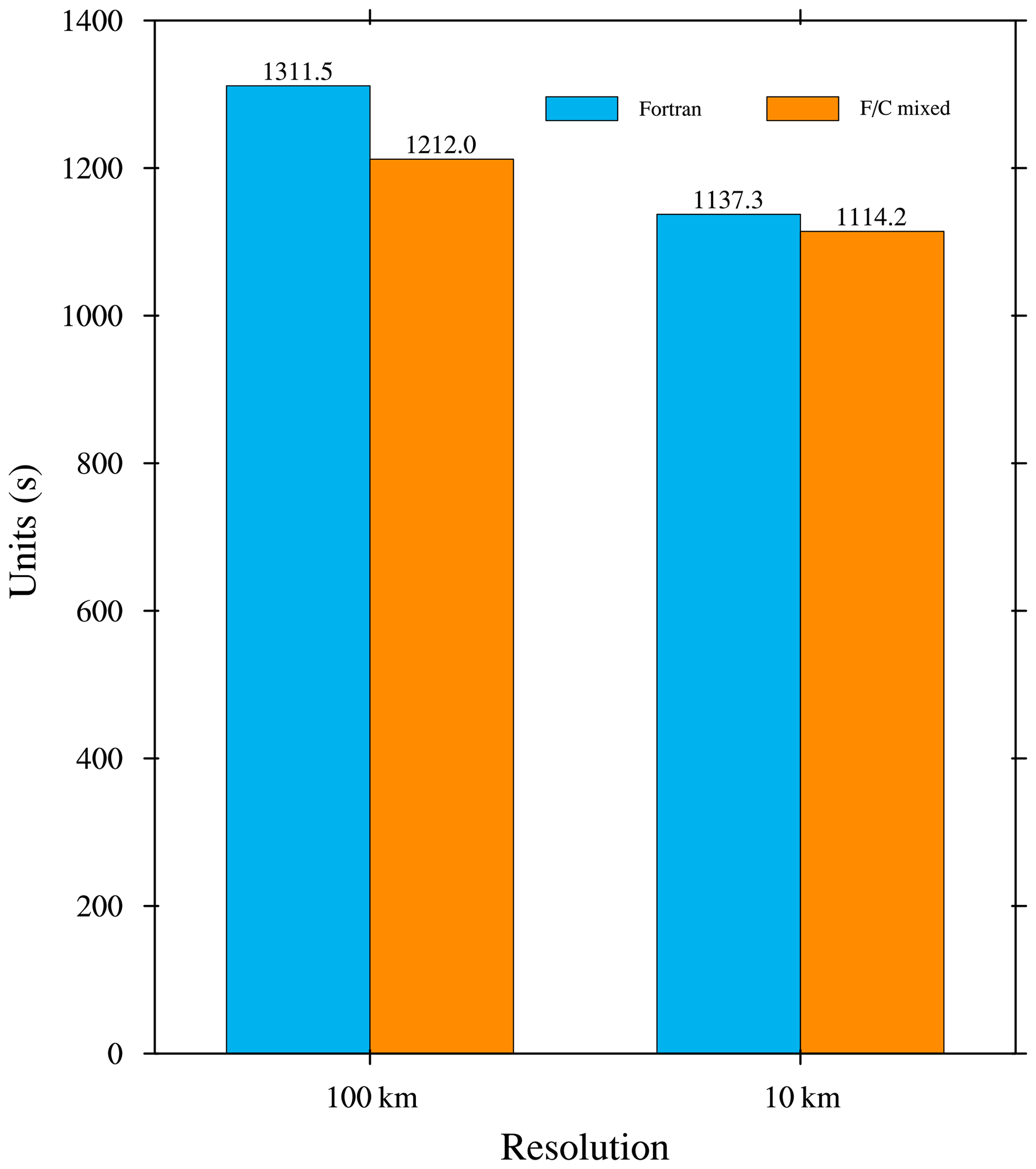
Figure 3 The wall clock time of a model day for the 10 km version and a model month for the 100 km version. The blue and orange bars are for the Fortran and Fortran and C mixed versions. These tests were conducted on an Intel Xeon CPU platform (E5-2697A v4, 2.60 GHz). We used 28 and 280 cores for the low and high resolutions, respectively.

This C transitional version becomes the starting point of HIP/C$++$ codes and reduces the complexity of developing the HIP version of LICOM3.

3.3 Optimization and tuning methods in LICOM3-HIP

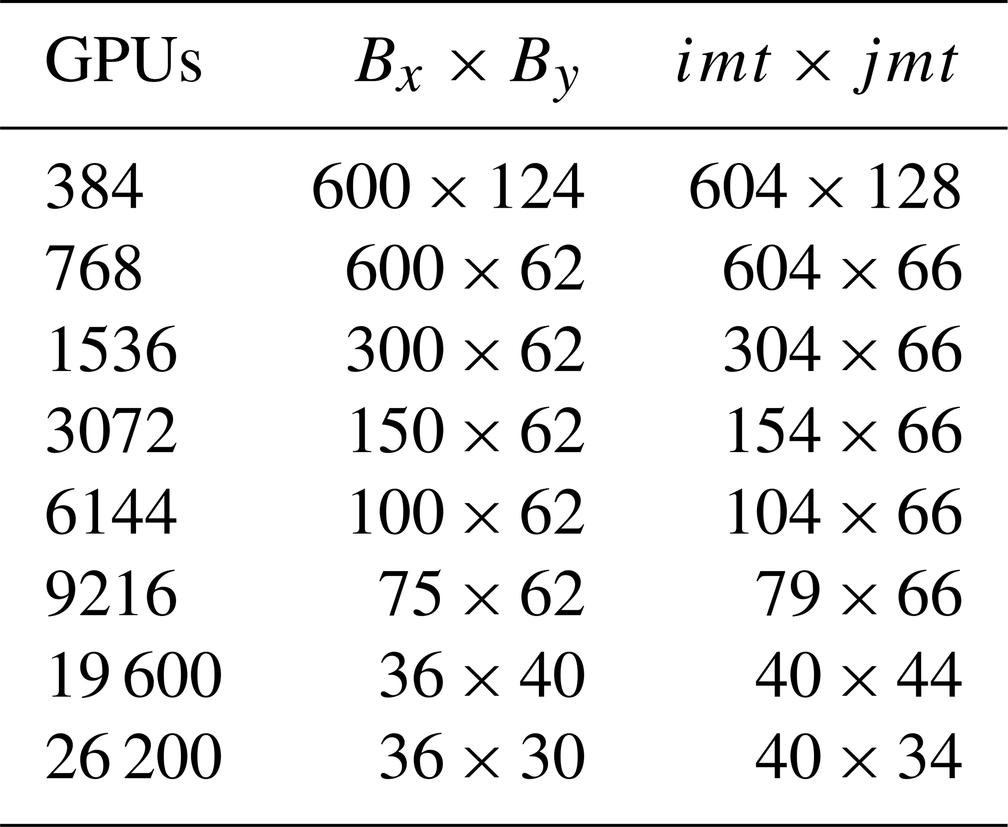
The unit of computation in LICOM3-HIP is a horizontal grid point. For example, $\mathrm{1}/\mathrm{20}{}^{\circ }$ corresponds to 7200×3920 grids. For the convenience of MPI parallelism, the grid points are grouped as blocks; that is, if Proc_x×Proc_y MPI processes are used in the x and y directions, then each block has B_x×B_y grids, where $\text{Pro}{c}_x\times B_x=\mathrm{7200}$ and $\text{Pro}{c}_y\times B_y=\mathrm{3920}$. Each GPU process performs two-dimensional (2-D) or three-dimensional (3-D) computations in these B_x×B_y grids, which is similar to the MPI process. Two-dimensional means that the grids are partitioned only in the horizontal directions, and 3-D includes also the depth or vertical direction. In practice, four lateral columns are added to B_x and B_y (two on each side, $imt=B_x+\mathrm{4}$, $jmt=B_y+\mathrm{4}$) for the halo. Table 2 lists the frequently used block definitions of LICOM3.

Table 2 Block partition for the $\mathrm{1}/\mathrm{20}{}^{\circ }$ setup.

The original LICOM3 was written in F90. To adapt it to a GPU, we applied Fortran–C hybrid programming. As shown in Fig. 2, the codes are kept using the F90 language before entering device stepon and after stepon out. The core computation processes within the stepons are rewritten using HIP/C. Data structures in the CPU space remain the same as the original Fortran structures. The data commonly used by F90 and C are then defined by extra C, including files, and defined by “extern”-type pointers in C syntax to refer to them. In the GPU space, newly allocated GPU global memories hold the arrival correspondence with those in the CPU space, and the HipMemcpy is called to copy them in and out.

Seven major subroutines (including their sub-recurrent calls) are converted from Fortran to HIP. The seven subroutine call sequences are maintained, but each subroutine is deeply recoded in the HIP to obtain the best performance. The CPU space data are 2-D or 3-D arrays; in the GPU space, they are changed to 1-D arrays to improve the data transfer speed between different GPU subroutines.

LICOM3-HIP is a two-level parallelism, and each MPI process corresponds to an ocean block. The computation within one MPI process is then pushed into the GPU. The latency of the data copy between the GPU and CPU is one of the bottlenecks for daily computation loops. All read-only GPU variables are allocated and copied at the initial stage to reduce the data copy time. Some data copy is still needed in the stepping loop, e.g., an MPI call in barotr.cpp.

Figure 4 The code using temporary arrays to avoid data dependency.

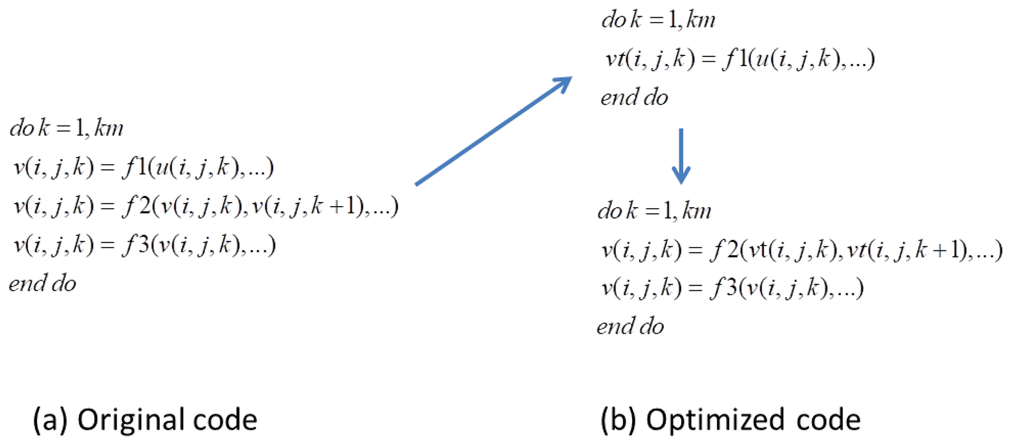
The computation block in MPI (corresponding to 1 GPU) is a 3-D grid; in the HIP revision, 3-D parallelism is implemented. This change adds more parallels inside one block than the MPI solo parallelism (only 2-D). Some optimizations are needed to adapt to this change, such as increasing the global arrays to avoid data dependency. A demo for using a temporary array to parallelize the computation inside a block is shown in Fig. 4. Figure 4a represents a loop of the original code in the k direction. Since the variable $v(i,j,k)$ has a dependence on $v(i,j,k+\mathrm{1})$, it will cause an error when the GPU threads are parallel in the k direction. We then separate the variable into two HIP kernel computations. In the upper part of Fig. 4b, a temporary array vt is used to hold the result of f1(), and this can be GPU threads that are parallel in the k direction. Then, at the bottom of Fig. 4b, we use vt to perform the computations of f2() and f3(); this can still be GPU threads that are parallel in the k direction. Finally, this loop of codes is parallelized.

Parallelization in a GPU is similar to a shared-memory program; memory write conflicts occur in the subroutine tracer advection computation. We change the if–else tree in this subroutine; hence, the data conflicts between neighboring grids are avoided, making the 3-D parallelism successful. Moreover, in this subroutine, we use more operations to alternate the data movement to reduce the cache usage. Since the operation can be GPU thread parallelized and will not increase the total computation time, reducing the memory cache improves this subroutine's final performance.

A notable problem when the resolution is increased to $\mathrm{1}/\mathrm{20}{}^{\circ }$ is that the total size of Fortran common blocks will be larger than 2 GB. This change will not cause abnormalities for C in the GPU space. However, if the GPU process references the data, the system call in HipMemcpy will cause compilation errors (perhaps due to the compiler limitation of the GPU compilation tool). We can change the original Fortran arrays' data structure from the “static” to the “allocatable” type in this situation. Since a GPU is limited to 16 GB GPU memory, the ocean block size in one block should not be too large. In practice, the $\mathrm{1}/\mathrm{20}{}^{\circ }$ version starts from 384 GPUs (and is regarded as the baseline for speedup here); if the partition is smaller than that value, sometimes insufficient GPU memory errors will occur.

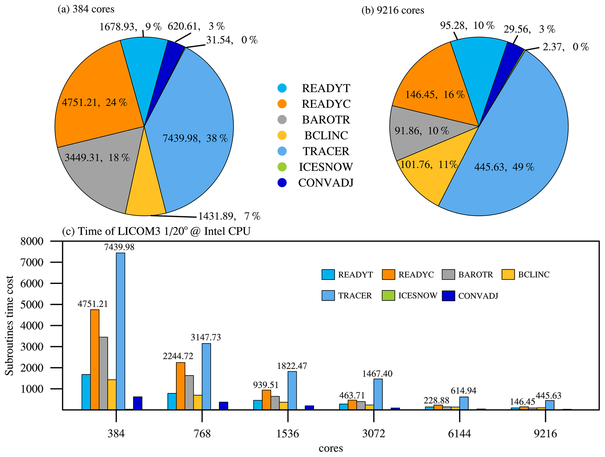
Figure 5 The seven core subroutines' time cost percentages for (a) 384 and (b) 9216 CPU cores. (c) The subroutines' time cost at different scales of LICOM3 ($\mathrm{1}/\mathrm{20}{}^{\circ }$). These tests were conducted on an Intel Xeon CPU platform (E5-2697A v4, 2.60 GHz).

Table 3 The number calls of halos in LICOM3 subroutines for each step.

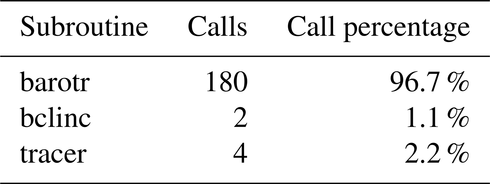
We found that the tracer is the most time-consuming subroutine for the CPU version (Fig. 5). With the increase in CPU cores from 384 to 9216, the ratio of cost time for the tracer also increases from 38 % to 49 %. The subroutines readyt and readyc are computing-intensive. The subroutine tracer is both a computing-intensive and communication-intensive, and barotr is a communication-intensive subroutine. The communication of barotr is 45 times more than that of tracer (Table 3). Computing-intensive subroutines can achieve good GPU speed, but communication-intensive subroutines will achieve poor performance. The superlinear speedups for tracer and readyc might be mainly caused by memory use, in which the memory use of each thread for 768 GPU cards is only half for 384 GPU cards.

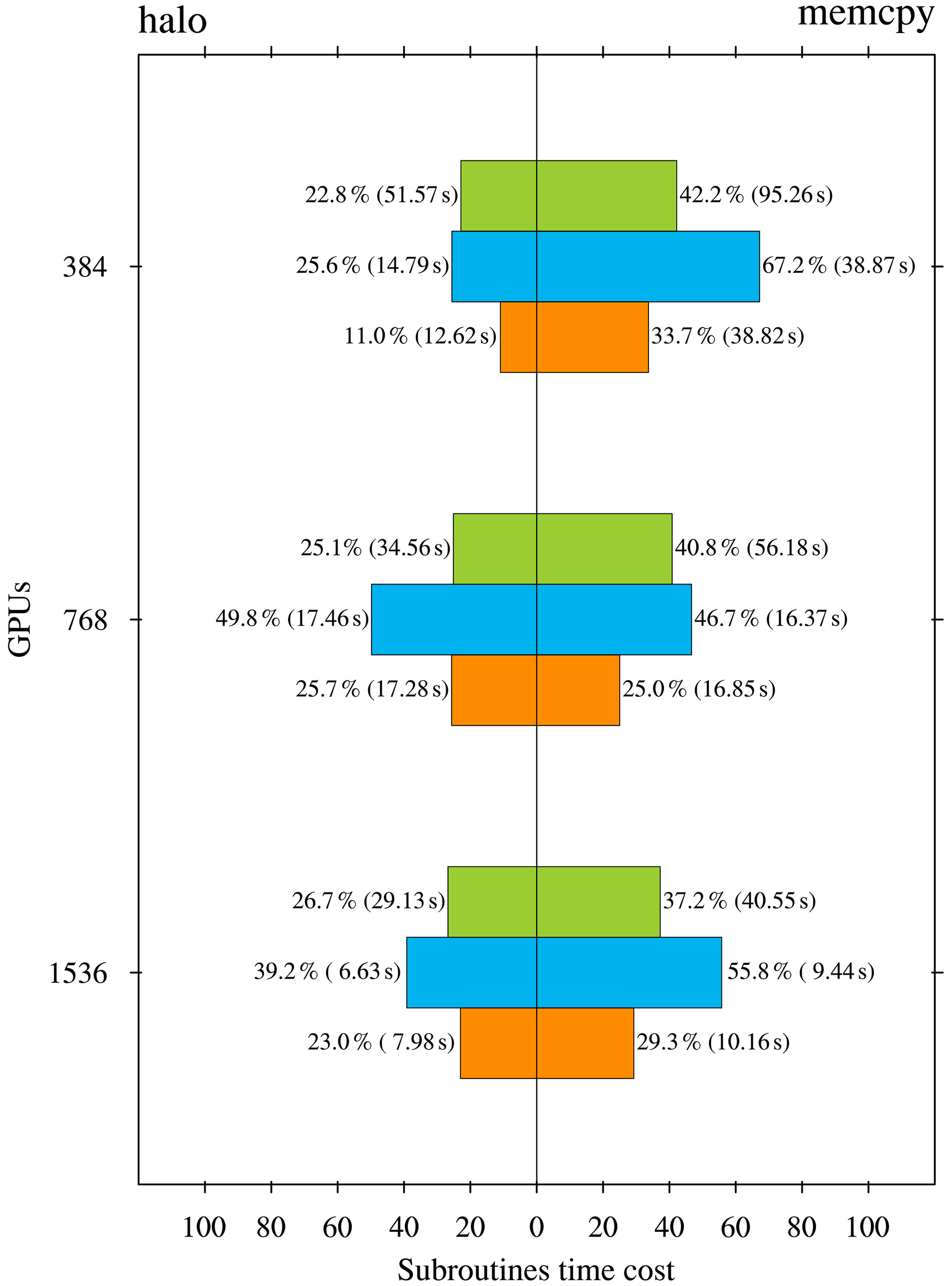
Figure 6 The ratio of the time cost of halo update and memory copy to the total time cost for the three subroutines, barotr (green), bclinc (blue), and tracer (orange), in the HIP version LICOM for three scales (unit: %). The numbers in the blankets are the time cost of the two processes (unit: s).

We performed a set of experiments to measure the time cost of both halo update and memory copy in the HIP version (Fig. 6). These two processes in the time integration are conducted in three subroutines: barotr, bclinc, and tracer. The figure shows that barotr is the most time-consuming subroutine, and the memory copy dominates, which takes approximately 40 % of the total time cost.

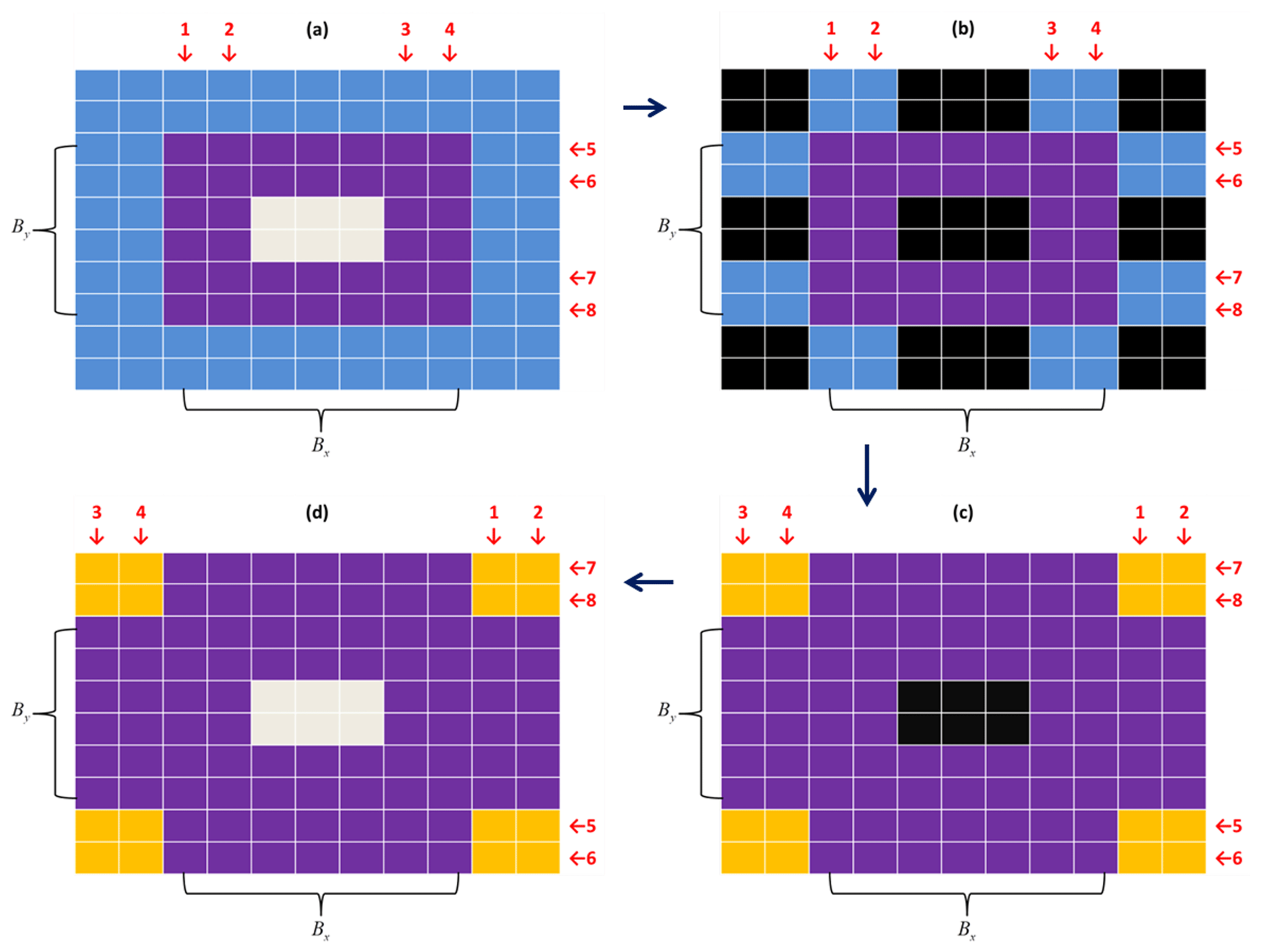
Figure 7 The lateral packing (only transferring four rows and four columns of data between the GPU and CPU) method to accelerate the halo. (a) In the GPU space, where central (gray) grids are unchanged; (b) transferred to the CPU space, where black grids mean no data; (c) after halo with neighbors; and (d) transfer back to the GPU space.

Data operations inside CPU (or GPU) memory are at least 1 order of magnitude faster than the data transfer between GPU and CPU through 16X PCI-e. Halo exchange at the MPI level is similar to POP (Jiang et al., 2019). We did not change these codes in the HIP version. The four blue rows and columns in Fig. 7 demonstrate the data that need to be exchanged with the neighbors. As shown in Fig. 7, in GPU space, we pack the necessary lateral data for halo operation from imt×jmt to 4(imt+jmt). This change reduces the HipMemcpy data size to $(\mathrm{4}/imt+\mathrm{4}/jmt)$ of the original one. The larger that imt and jmt are, the less data are transferred. At 384 GPUs, this change saves approximately 10 % of the total computation time. The change is valuable for the HIP since the platform has no CUDA-aware MPI installed; otherwise, the halo operation can be done in the GPU space directly as done by POM.gpu (Xu et al., 2015). The test indicates that the method can decrease approximately 30 % of the total wall clock time of barotr when 384 GPUs are used. However, we have not optimized other kernels so far because their performance is not as good as 384 GPUs when the GPU scale exceeds 10 000. We keep it here as an option to improve the performance of barotr at operational scales (i.e., GPU scales under 1536).

3.4 Model I$/$O (input$/$output) optimization

Approximately 3 GB forcing data are read from the disk every model year, while approximately 60 GB daily mean predicted variables are stored to disk every model day. The time cost for reading daily forcing data from the disk increased to 200 s in 1 model day after the model resolution increased from 1 to $\mathrm{1}/\mathrm{20}{}^{\circ }$. This time is comparable to the wall clock time for one model step when 1536 GPUs are applied; hence, we must optimize the model for total speedup. The cause of low performance is daily data reading and scattering to all nodes every model day; we then rewrite the data reading strategy and perform parallel scattering for 10 different forcing variables. Originally, 10 variables are read from 10 files, interpolated to a $\mathrm{1}/\mathrm{20}{}^{\circ }$ grid, and then scattered to each processor or thread. All the processes are sequentially done at the master processor. In the revised code, we use 10 different processes to read, interpolate, and scatter in parallel. Finally, the time cost of input is reduced to approximately 20 s, which is $\mathrm{1}/\mathrm{10}$ of the original time cost (shown below).

As indicated, the time cost for one integration step (excluding the daily mean and I$/$O) is approximately 200 s using 1536 GPUs. One model day's output needs approximately 250 s; this is also beyond the GPU computation time for one step. We modify the subroutine to a parallel version, which decreases the data write time to 70 s on the test platform (this also depends on system I$/$O performance).

4 Model performance

4.1 Model performance in computing

Performing kilometer-scale and global climatic simulations is challenging (Palmer, 2014; Schär et al., 2020). As specified by Fuhrer et al. (2018), the SYPD is a useful metric to evaluate model performance for a parallel model (Balaji et al., 2017). Because a climate model often needs to run for at least 30–50 years for each simulation, at a speed of 0.2–0.3 SYPD, the time will be too long to finish the experiment. The common view is that at least 1–2 SYPD is an adequate entrance for a realistic climate study. It also depends on the timescale in a climate study. For example, for the 10–20-year simulation, 1–2 SYPD seems acceptable, and for the 50–100-year simulation, 5–10 SYPD is better. The NCEP weather prediction system throughput standard is 8 min to finish 1 model day, equivalent to 0.5 SYPD.

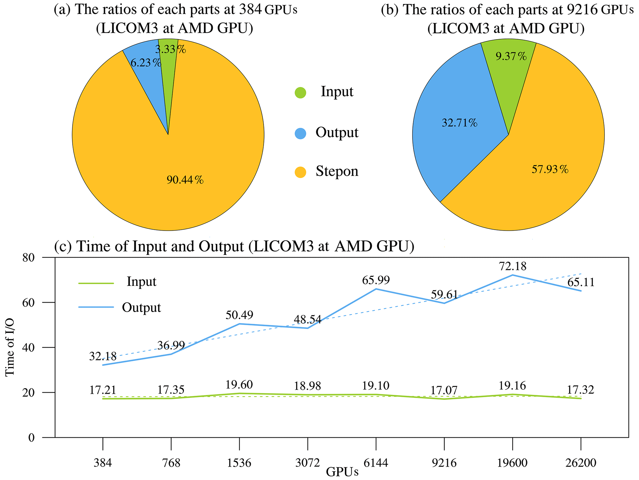
Figure 8 (a) The 384 GPUs and (b) 9216 GPUs, with the I$/$O ratio in total simulation time for the $\mathrm{1}/\mathrm{20}{}^{\circ }$ setup, and (c) the changes in I$/$O times vs. different GPUs.

Figure 8 illustrates the I$/$O performance of LICOM3-HIP, comparing the performances of computation processes. When the model applies 384 GPUs, the I$/$O costs $\mathrm{1}/\mathrm{10}$ of the total simulation time (Fig. 8a). When the scale increases to 9216 GPUs, the I$/$O time increases but is still smaller than the GPU's step time (Fig. 8b). The improved LICOM3 I$/$O in total costs approximately 50–90 s (depending on scales), especially when the input remains stable (Fig. 8c) while scaling increases. This optimization of I$/$O ensures that LICOM3-HIP $\mathrm{1}/\mathrm{20}{}^{\circ }$ runs well at all practice scales for a realistic climate study. The I$/$O time was cut off from the total simulation time in the follow-up test results to analyze the purely parallel performance.

Figure 9 Roofline model for the AMD GPU and the performance of LICOM's main subroutines.

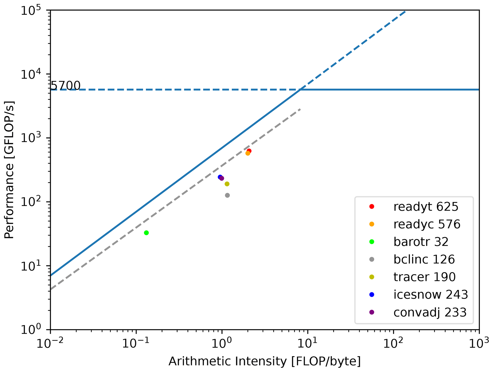
Figure 9 shows the roofline model using the Stream GPU and the LICOM program's measured behavioral data on a single computation node bound to one GPU card depicting the relationship between arithmetic intensity and performance floating point operations. The 100 km resolution case is employed for the test. The blue and gray oblique lines are the fitting lines related to the Stream GPU program's behavioral data using 5.12×10⁸ and 1×10⁶ threads, respectively, both with a block size of 256, which attain the best configuration. For details, the former is approximately the maximum thread number restricted by GPU card memory, achieving a bandwidth limit of 696.52 GB s⁻¹. In comparison, the latter is close to the average number of threads in GPU parallel calculations used by LICOM, reaching a bandwidth of 344.87 GB s⁻¹ on average. Here, we use the oblique gray line as a benchmark to verify the rationality of LICOM's performance, accomplishing an average bandwidth of 313.95 GB s⁻¹.

Due to the large calculation scale of the entire LICOM program, the divided calculation grid bound to a single GPU card is limited by video memory; most kernel functions issue no more than 1.2×10⁶ threads. As a result, the floating-point operation performance is a little far from the oblique roofline shown in Fig. 9. In particular, the subroutine bclinc apparently strays away from the entire trend for including frequent 3-D array Halo MPI communications, and much data transmission occurs between the CPU and GPU.

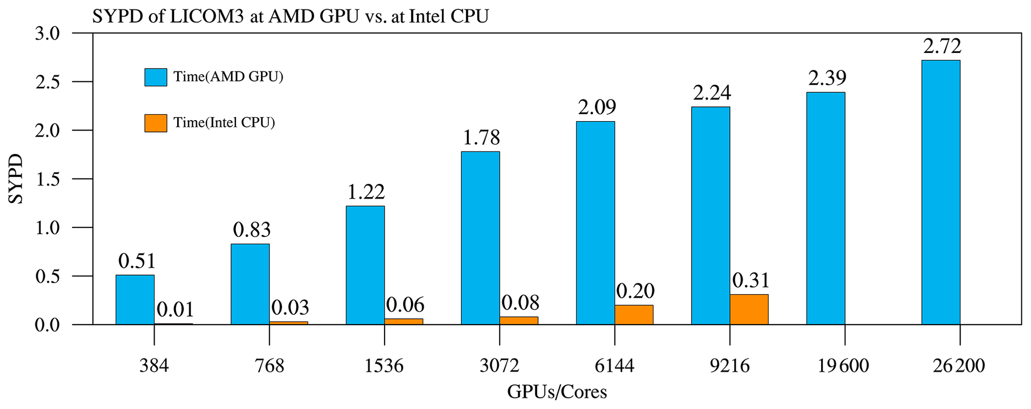
Figure 10 Simulation performances of the AMD GPU vs. Intel CPU core for LICOM3 ($\mathrm{1}/\mathrm{20}{}^{\circ }$). Unit: SYPD.

Figure 10 shows the SYPD at various parallel scales. The baseline (384) of GPUs could achieve a 42 times faster speedup than that of the same number of CPU cores. Sometimes, we also count the overall speedup for 384 GPUs in 96 nodes vs. the total 3072 CPU cores in 96 nodes. We can obtain an overall performance speedup of 384 or approximately 6–7 times. The figure also indicates that for all scales, the SYPD continues to increase. On the scale of 9216 GPUs, the SYPD first goes beyond 2, which is 7 times the same CPU result. A quasi-whole-machine (26 200 GPUs, $\mathrm{26}\mathrm{200}\times \mathrm{65}=\mathrm{1}\mathrm{703}\mathrm{000}$ cores in total, one process corresponds to one CPU core plus 64 GPU cores) result indicates that it can still obtain an increasing SYPD to 2.72.

Since each node has 32 CPU cores and four GPUs, each GPU is managed by one CPU thread in the present cases. We can also quantify GPUs' speedup vs. all CPU cores on the same number of nodes. For example, 384 (768) GPUs correspond to 96 (192) nodes, which have 3072 (6144) CPU cores. Therefore, the overall speedup is approximately 6.375 ($\mathrm{0.51}/\mathrm{0.08}$) for 384 GPUs and 4.15 ($\mathrm{0.83}/\mathrm{0.2}$) for 768 GPUs (Fig. 10). The speedups are comparable with our previous work porting LICOM2 to GPU using OpenACC (Jiang et al., 2019), which is approximately 1.8–4.6 times the speedup using one GPU card vs. two eight-core Intel GPUs in small-scale experiments for specific kernels. Our results are also slightly better than in Xu et al. (2015), who ported another ocean model to GPUs using Cuda C. However, due to the limitation of the number of Intel CPUs (maximum of 9216 cores), we did not obtain the overall speedup for 1536 and more GPUs.

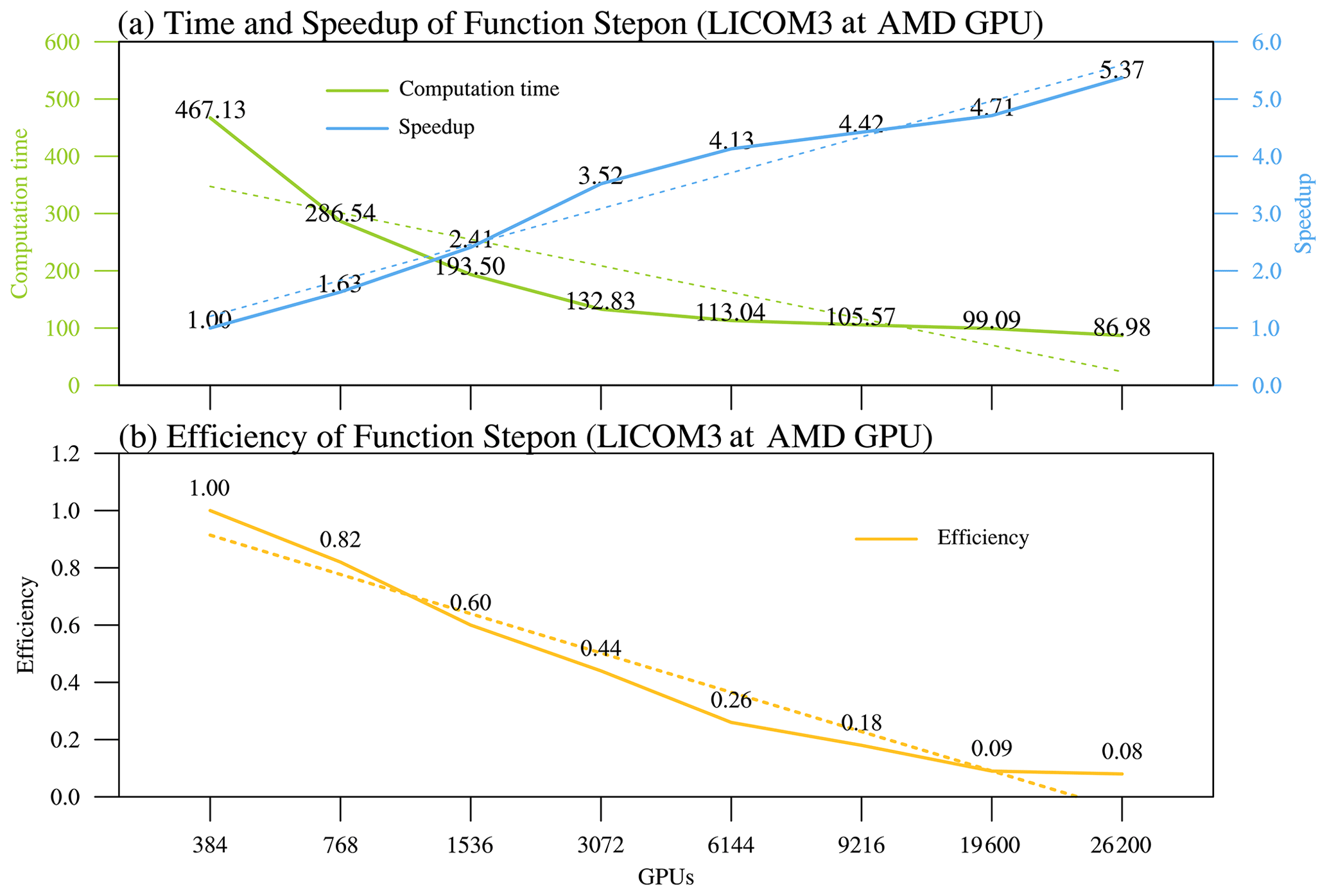
Figure 11 (a) Computation time (green) and speedup (blue) and (b) parallel efficiency (orange) at different scales for stepons of LICOM3-HIP ($\mathrm{1}/\mathrm{20}{}^{\circ }$).

Figure 11 depicts the actual times and speedups of different GPU computations. The green line in Fig. 11a is a function of the stepon time cost; it decreases while the GPU number increases. The blue curve of Fig. 11a shows the increase in speedup with the rise in the GPU scale. Despite the speedup increase, the efficiency of the model decreases. At 9216 GPUs, the model efficiency starts under 20 %, and for more GPUs (19 600 and 26 200), the efficiency is flattened to approximately 10 %. The efficiency decrease is mainly caused by the latency of the data copy in and out to the GPU memory. For economic consideration, the 384–1536 scale is a better choice for realistic modeling studies.

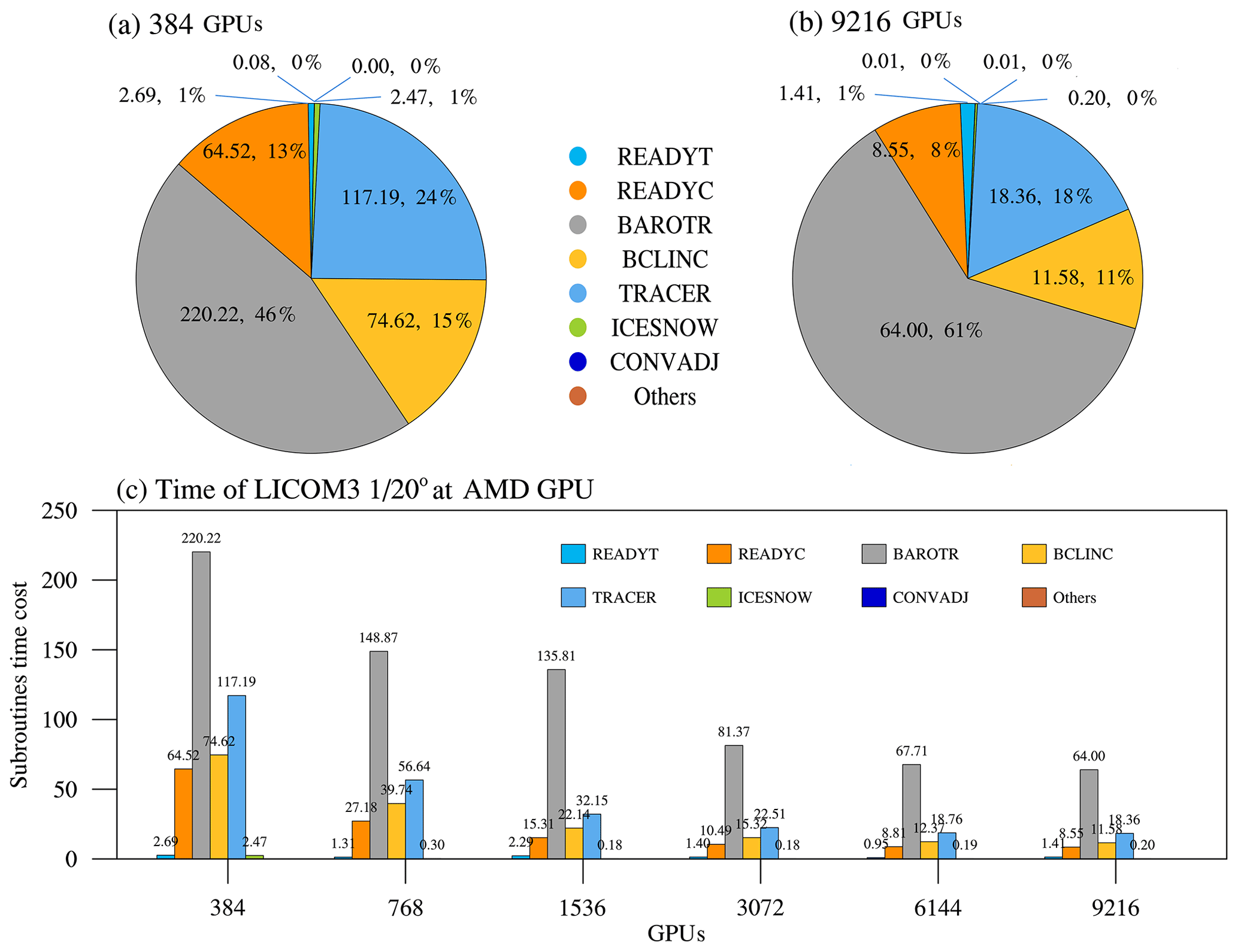
Figure 12 The seven core subroutines' time cost percentages for (a) 384 GPUs and (b) 9216 GPUs. (c) The subroutines' time cost at different scales of LICOM3-HIP ($\mathrm{1}/\mathrm{20}{}^{\circ }$).

Figure 12 depicts the time cost of seven core subroutines of LICOM3-HIP. We find that the top four most time-costly subroutines are barotr, tracer, bclinc, and readyc, and the other subroutines cost only approximately 1 % of the whole computation time. When 384 GPUs are applied, the barotr costs approximately 50 % of the total time (Fig. 12a), which solves the barotropic equations. When GPUs are increased to 9216, each subroutine's time cost decreases, but the percentage of subroutine barotr is increased to 62 % (Fig. 12b). As mentioned above, this phenomenon can be interpreted by having more haloing in barotr than in the other subroutines; hence, the memory data copy and communication latency make it slower.

4.2 Model performance in climate research

The daily mean sea surface height (SSH) fields of the CPU and HIP simulations are compared to test the usefulness of the HIP version of LICOM for the numerical precision of scientific usage. Here, the results from $\mathrm{1}/\mathrm{20}{}^{\circ }$ experiments on a particular day (1 March of the fourth model year) are used (Fig. 13a and b). The general SSH spatial patterns of the two are visually very similar. Significant differences are only found in very limited areas, such as in the eddy-rich regions near strong currents or high-latitude regions (Fig. 13c); in most places, the difference in values fall into the range of −0.1 and 0.1 cm. Because the hardware is different and the HIP codes' mathematical operation sequence is not always the same as that for the Fortran version, the HIP and CPU versions are not identical byte-by-byte. Therefore, it is hard to verify the correctness of the results from the HIP version. Usually, the ensemble method is employed to evaluate the consistency of two model runs (Baker et al., 2015). Considering the unacceptable computing and storage resources, in addition to the differences between the two versions, we simply compute root mean square errors (RMSEs) between the two versions, which are only 0.18 cm, much smaller than the spatial variation of the system, which is 92 cm (approximately 0.2 %). This indicates that the results of LICO3-HIP are generally acceptable for research.

Figure 13 Daily mean simulated sea surface height for (a) CPU and (b) HIP versions of LICOM3 at $\mathrm{1}/\mathrm{20}{}^{\circ }$ on 1 March of the fourth model year. (c) The difference between the two versions (HIP minus CPU). Units: cm.

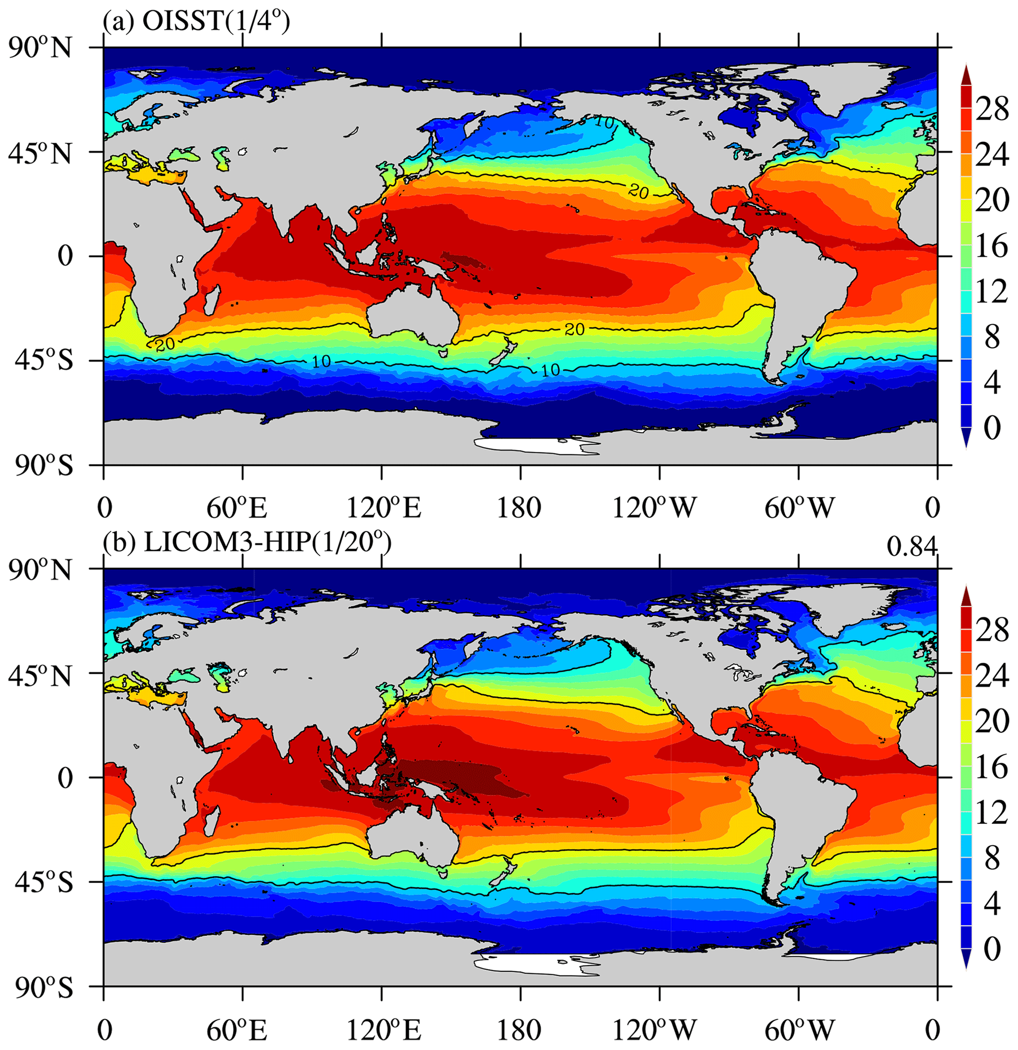
Figure 14 (a) Observed annual mean sea surface temperature in 2016 from the Optimum Interpolation Sea Surface Temperature (OISST); (b) simulated annual mean SST for LICOM3-HIP at $\mathrm{1}/\mathrm{20}{}^{\circ }$ during model years 0005–0014. Units: ^∘C.

The GPU version's sea surface temperature (SST) is compared with the observed SST to evaluate the global $\mathrm{1}/\mathrm{20}{}^{\circ }$ simulation's preliminary results from LICOM3-HIP (Fig. 14). Because the LICOM3-HIP experiments are forced by the daily mean atmospheric variables in 2016, we also compare the outputs with the observation data in 2016. Here, the $\mathrm{1}/\mathrm{4}{}^{\circ }$ Optimum Interpolation Sea Surface Temperature (OISST) is employed for comparison, and the simulated SST is interpolated to the same resolution as the OISST. We find that the global mean values of SST are close together but with a slight warming bias of 18.49 ^∘C for observations vs. 18.96 ^∘C for the model. The spatial pattern of SST in 2016 is well reproduced by LICOM3-HIP. The spatial standard deviation (SD) of SST is 11.55 ^∘C for OISST and 10.98 ^∘C for LICOM3-HIP. The RMSE of LICOM3-HIP against the observation is only 0.84 ^∘C.

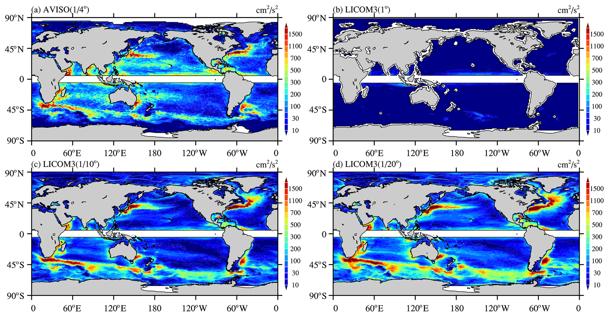
Figure 15 (a) Observed annual mean eddy kinetic energy (EKE) in 2016 from AVISO (Archiving, Validation and Interpretation of Satellite Oceanographic). Simulated annual mean SST in 2016 for LICOM3-HIP at (b) 1^∘, (c) $\mathrm{1}/\mathrm{10}{}^{\circ }$, and (d) $\mathrm{1}/\mathrm{20}{}^{\circ }$. Units: cm² s⁻².

With an increasing horizontal resolution of the observations, we now know that mesoscale eddies are ubiquitous in the ocean at the 100–300 km spatial scale. Rigorous eddies usually occur along significant ocean currents, such as the Kuroshio and its extension, the Gulf Stream, and the Antarctic Circumpolar Current (Fig. 15a). Eddies also capture more than 80 % of the ocean's kinetic energy, which was estimated using satellite data (e.g., Chelton et al., 2011). Therefore, these mesoscale eddies must be solved in the ocean model. A numerical model's horizontal resolution must be higher than $\mathrm{1}/\mathrm{10}{}^{\circ }$ to resolve the global ocean eddies but cannot resolve the eddies in high-latitude and shallow waters (Hallberg, 2013). Therefore, a higher resolution is required to determine the eddies globally. The EKE for the 1^∘ version is low, even in the areas with strong currents, while the $\mathrm{1}/\mathrm{10}{}^{\circ }$ version can reproduce most of the eddy-rich regions in the observation. The EKE increases when the resolution is further enhanced to $\mathrm{1}/\mathrm{20}{}^{\circ }$, indicating that many more eddy activities are resolved.

5 Discussion

5.1 Application of the ocean climate model beyond 10 000 GPUs

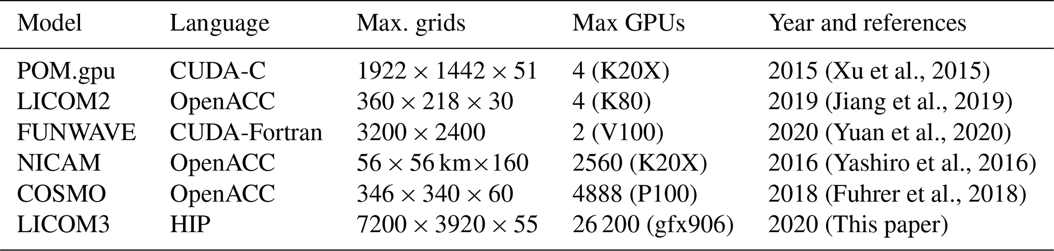
Table 4 summarizes the detailed features of some published GPU version models. We find that various programming methods have been implemented for different models. A near-kilometer atmospheric model using 4888 GPUs was reported as a large-scale example of weather/climate studies. With supercomputing development, the horizontal resolution of ocean circulation models will keep increasing, and more sophisticated physical processes will also be developed. LICOM3-HIP has a larger scale, not only in terms of grid size but also in final GPU numbers.

Table 4 Some GPU versions of weather/climate models.

We successfully performed a quasi-whole-machine (26 200 GPUs) test, and the results indicate that the model obtained an increasing SYPD (2.72). The application of an ocean climate model beyond 10 000 GPUs is not easy because running the multi-nodes plus multi-GPUs requires that the network connection, PCI-e and memory speed, and input$/$output storage systems all work to their best performances. Gupta et al. (2017) investigated 23 types of system failures to improve the reliability of the HPC (high-performance computing) system. Unlike in Gupta's study, only the three most common types of failures we encountered are discussed here. The three most common errors when running LICOM3-HIP are MPI hardware errors, CPU memory access errors, and GPU hardware errors. Let us suppose that the probability of an individual hardware (or software) error occurring is 10⁻⁵ (which means one failure in 100 000 h). As the MPI (GPU) scale increases, the total error rate increases, and once a hardware error occurs, the model simulation will fail.

Table 5 Success and failure rates of different scales for 1 wall clock hour simulation.

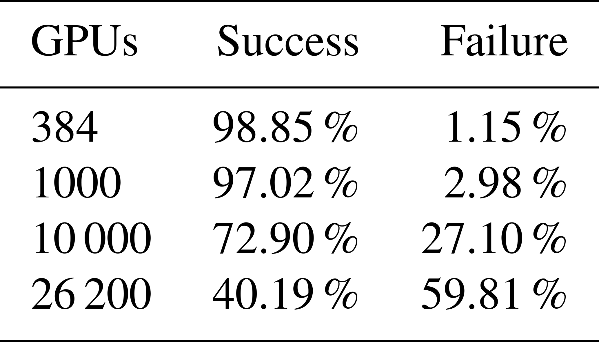
When 384 GPUs are applied, the success rate within 1 h can be expressed as $(\mathrm{1}-\mathrm{384}\times {\mathrm{10}}^{-\mathrm{5}}{)}^{\mathrm{3}}=\mathrm{98.85}\mathrm{\%}$, and the failure rate is then $\mathrm{1}-(\mathrm{1}-\mathrm{384}\times {\mathrm{10}}^{-\mathrm{5}}{)}^{\mathrm{3}}=\mathrm{1.15}\mathrm{\%}$. Applying this formula, we can obtain the failure rate corresponding to 1000, 10 000, and 26 200 GPUs. The results are listed in Table 5. As shown in Table 5, on the medium scale (i.e., 1000 GPUs are used), three failures will occur through 100 runs; when the scale increases to 10 000 GPUs, one-quarter of them will fail. The 10⁻⁵ error probability also indicates that 10 000 GPU tasks cannot run 10 continuous hours on average. If the success time restriction decreases, the model success rate will increase. For example, within 6 min, the 26 200 GPU task success rate is $(\mathrm{1}-\mathrm{26}\mathrm{200}\times {\mathrm{10}}^{-\mathrm{6}}{)}^{\mathrm{3}}=\mathrm{9234}\mathrm{\%}$, and its failure rate is $\mathrm{1}-(\mathrm{1}-\mathrm{26}\mathrm{200}\times {\mathrm{10}}^{-\mathrm{6}}{)}^{\mathrm{3}}=\mathrm{7.66}\mathrm{\%}$.

5.2 Energy to solution

We also measured the energy to solution here. A simulation-normalized energy (E) is employed here as a metric. The formula is as follows:

$${\displaystyle }E=\text{TDP}\times N\times \mathrm{24}/\text{SYPD},$$

where TDP is the thermal design power, N is the computer nodes used, and SYPD$/$24 equals the simulated years per hour. Therefore, the smaller the E value is, the better, which means that we can obtain more simulated years within a limited power supply. To calculate E's value, we estimated the TDP of 1380 W for a node on the present platform (one AMD CPU and four GPUs) and 290 W for a reference node (two Intel 16-core CPUs). We only include the TDP of CPUs and GPUs here.

Based on the above power measurements, the simulations' energy cost is calculated in megawatt-hours per simulation year (MWh SY⁻¹). The energy costs for the $\mathrm{1}/\mathrm{20}{}^{\circ }$ LICOM3 simulations running on CPUs and GPUs are comparable when the numbers of MPI processors are within 1000. The energy costs of LICOM3 at $\mathrm{1}/\mathrm{20}{}^{\circ }$ running on 384 (768) GPUs and CPUs are approximately 6.234 (7.661) MWh SY⁻¹ and 6.845 (6.280) MWh SY⁻¹, respectively. However, the simulation speed of LICOM3 on a GPU is much faster than that on a CPU: approximately 42 times faster for 384 processors and 31 times faster for 768 processors. When the number of MPI processors is beyond 1000, the value of E for the GPU becomes much larger than that for the CPU. This result indicates that the GPU is not fully loaded at this scale.

6 Conclusions

The GPU version of LICOM3 under the HIP framework was developed in the present study. Seven kernels within the time integration of the mode are all ported to the GPU, and 3-D parallelization (also partitioned in the vertical direction) is applied. The new model was implemented and gained an excellent acceleration rate on a Linux cluster with AMD GPU cards. This is also the first time an ocean general circulation model has been fully applied on a heterogeneous supercomputer using the HIP framework. In total, it took 19 months, five PhD students and five part-time staff to finish the porting and testing work.

Based on our test using the $\mathrm{1}/\mathrm{20}{}^{\circ }$ configuration, LICOM3-HIP is 42 times faster than the CPU when 384 AMD GPUs and CPU cores are used. LICOM3-HIP has good scalability, and can obtain a speedup of more than 4 on 9216 GPUs compared to 384 GPUs. The SYPD, which is in equilibrium with the speedup, continues to increase as the number of GPUs increases. We successfully performed a quasi-whole-machine test, which was 6550 nodes and 26 200 GPUs, using $\mathrm{1}/\mathrm{20}{}^{\circ }$ LICOM3-HIP on the supercomputer, and at the grand scale, the model can obtain an increasing SYPD of 2.72. The modification or optimization of the model also improves the 10 and 100 km performances, although we did not analyze their performances in this article.

The efficiency of the model decreases with the increasing number of GPUs. At 9216 GPUs, the model efficiency starts under 20 % against 384 GPUs, and when the number of GPUs reaches or exceeds 20 000, the efficiency is only approximately 10 %. Based on our kernel function test, the decreasing efficiency was mainly caused by the latency of data copy in and out to the GPU memory in solving the barotropic equations, particularly for the number of GPUs larger than 10 000.

Using the $\mathrm{1}/\mathrm{20}{}^{\circ }$ configuration of LICOM3-HIP, we conducted a 14-year spin-up integration. Because the hardware is different and the GPU codes' mathematical operation sequence is not always the same as that of the Fortran version, the GPU and CPU versions cannot be identical byte by byte. The comparison between the GPU and CPU versions of LICOM3 shows that the differences are minimal in most places, indicating that the results from LICOM3-HIP can be used for practical research. Further comparison with the observation and the lower-resolution results suggests that the $\mathrm{1}/\mathrm{20}{}^{\circ }$ configuration of LICOM3-HIP can reproduce the observed large-scale features and produce much smaller-scale activities than that of lower-resolution results.

The eddy-resolving ocean circulation model, which is a virtual platform for oceanography research, ocean forecasting, and climate prediction and projection, can simulate the variations in circulations, temperature, salinity, and sea level with a spatial scale larger than 15 km and a temporal scale from the diurnal cycle to decadal variability. As mentioned above, 1–2 SYPD is a good start for a realistic climate research model. The more practical GPU scale range for a realistic simulation is approximately 384–1536 GPUs. At these scales, the model still has 0.5–1.22 SYPD. Even if we decrease the loops in the barotr procedure to one-third of the original in the spin-up simulation, the performance will achieve 1–2.5 SYPD for 384–1536 GPUs. This performance will satisfy 10–50-year-scale climate studies. In addition, this version can be used for short-term ocean prediction in the future.

Additionally, the block size of $\mathrm{36}\times \mathrm{30}\times \mathrm{55}$ ($\mathrm{1}/\mathrm{20}{}^{\circ }$ setup, 26 200 GPUs) is not an enormous computational task for one GPU. Since one GPU has 64 cores and a total of 2560 threads, if a subroutine computation is 2-D, each thread's operation is too small. Even for the 3-D loops, it is still not large enough to load the entire GPU. This indicates that it will gain more speedup when the LICOM resolution is increased to the kilometer level. The LICOM3-HIP codes are now written for $\mathrm{1}/\mathrm{20}{}^{\circ }$, but they are kilometer-ready GPU codes.

The optimization strategies here are mostly at the program level and do not treat the dynamic or physics parts separately. We only ported all seven core subroutines to the GPU together, i.e., including both the dynamic and physics parts, within the time integration loops. Unlike atmospheric models, there are a few time-consuming physical processes in ocean models, such as radiative transportation, clouds, precipitation, and convection processes. Therefore, the two parts are usually not separated in the ocean model, particularly in the early stage of model development. This is also the case for LICOM. Further optimization to explicitly separate the dynamic core and the physical package is necessary in the future.

There is still potential to further increase the speedup of LICOM3-HIP. The bottleneck is in the high-frequency data copy in and out to the GPU memory in the barotropic part of LICOM3. Unless HIP-aware MPI is supported, the data transfer latency between the CPU and GPU cannot be overcome. Thus far, we can only reduce the time consumed by decreasing the frequency or magnitude of the data copy and even modifying the method to solve the barotropic equations. Additionally, using single precision within the time integration of LICOM3 might be another solution. The mixing-precision method has already been tested using an atmospheric model, and the average gain in computational efficiency is approximately 40 % (Váňa et al., 2017). We would like to try these methods in the future.