Beyond behavioural models: equifinality and overparameterisation undermine confidence in predictions by soil organic matter models

The complexity of soil organic matter models is often not supported by sufficient data for parameter optimisation, resulting in the calibration of more parameters than can be reliably optimised with the available data. This leads to equifinality, the phenomenon that multiple parameter sets generate behavioural models, i.e., similarly well-performing models that cannot be ruled out. As such trade-offs between model complexity and data availability are often overlooked for soil organic matter models, the aim of this study is to assess how equifinality affects the variability of predictions made by behavioural soil organic matter models. The results show that for the model used in this study, the number of identifiable parameters, those that do not compensate for one another, increases with the number of calibration constraints. However, this number remained limited to five even under the most data-rich scenario considered, including the C and N content of particulate organic matter (POM) and mineral-associated organic matter (MAOM) and their ¹⁴C signatures. Furthermore, the size of POM and MAOM could only be accurately simulated when data on these pool sizes were used to optimise parameters, while the turnover rate of MAOM was reliably simulated only when Δ¹⁴C data for MAOM were used. Regardless of the type of mathematical equations (e.g., absolute vs. relative Michaelis–Menten kinetics), or the number of optimised parameters, the tested models were able to correctly reproduce the measurements in steady state. However, different model structures led to divergent predictions upon a doubling of organic matter inputs, while the variation in the response of the behavioural models was up to eight times larger for overparameterised models compared to models for which only identifiable parameters were optimised. These results emphasise the necessity of optimising only identifiable model parameters to avoid hidden uncertainty in model predictions.

1 Introduction

When developing environmental models, including soil organic matter (SOM) models, the mechanistic understanding of ecosystem processes is translated into mathematical equations with multiple parameters. Such models are valuable research tools, and are used to test scientific hypotheses (e.g., Laub et al., 2024; Van de Broek et al., 2024; Tang and Riley, 2015), extrapolate ecosystem properties over larger spatial and temporal scales (e.g., Tao et al., 2023; Wieder et al., 2024), support policy decisions (e.g., Campbell and Paustian, 2015), and make predictions of ecosystem properties into the future under variable external forcings (e.g., Sulman et al., 2018; Pallandt et al., 2025). Model developers need to account for the complexity and high spatial variability in ecosystem properties (e.g., Nearing et al., 1999), which often cannot be quantified due to a lack of experimental and observational data across space and time (Schindler and Hilborn, 2015; Oreskes et al., 1994). As a consequence, there is a trade-off between model complexity and data availability that determines the overall model error (Van Rompaey and Govers, 2002). On the one hand, a model that does not include the most basic processes relevant to the simulated system has limited scientific and practical use. On the other hand, a model including processes for which the parameter values have not been measured or reliably estimated will be similarly unreliable. This led authors of articles presenting mechanistic SOM models to acknowledge that their proposed model structures could not be sufficiently tested because of a lack of data (Riley et al., 2014; Dwivedi et al., 2017). Thus, complex models do not necessarily outperform more simple models (Jakeman and Hornberger, 1993; Manzoni and Porporato, 2009; Perretti et al., 2013; Lawrence et al., 2009), and striking a balance between model complexity and data availability is a prerequisite to develop environmental models that can be applied reliably (Manzoni and Schimel, 2024; Lennon et al., 2024; Famiglietti et al., 2021).

Three concepts that are valuable to identify the mismatch between model complexity and data availability are identifiability, equifinality and overparameterisation. The concept of identifiability has a long history in scientific research (Rothenberg, 1971; Reiersøl, 1950), with different aspects of identifiability being defined and studied (Travis and Haddock, 1981; Delforge, 1977; Cobelli et al., 1979; Kleissen et al., 1990; DiStefano and Cobelli, 1980). The two aspects of identifiability that have been most frequently applied to environmental models are structural identifiability and practical identifiability. The concept of structural identifiability was first introduced by Bellman and Åström (1970). As a practical definition, a structural identifiability analysis assesses whether a unique set of parameter values can be obtained given a mathematical model structure without consideration of the available data (therefore also termed a priori identifiability). For example, the Michaelis–Menten equation (both the forward and backward formulations) to simulate the depolymerisation of organic matter or the uptake of dissolved organic matter by microbes is widely used in SOM models (Chandel et al., 2023). This equation contains one parameter in the numerator (the maximum process rate, V_max) and one in the denominator (the half-saturation constant, K_m). This implies that an infinite number of combinations for V_max and K_m can result in the same output by compensating for each other, rendering these parameters non-identifiable when optimised together (Sierra et al., 2015; Holmberg, 1982; Marschmann et al., 2019). More recently, practical identifiability analysis (Lam et al., 2022), also termed parameter identifiability analysis (Guillaume et al., 2019), has gained importance. This assesses whether a unique set of model parameters can be found given a combination of the model structure, available (calibration) data, and data uncertainty (therefore also termed a posteriori identifiability). It is the latter type of identifiability that will be assessed in the present study. Detailed information is present in the literature about the concepts of structural identifiability (Nguyen and Wood, 1982; Beck, 1987; Walter and Pronzato, 1996) and practical identifiability (Lam et al., 2022; Guillaume et al., 2019), or both combined (Wanika et al., 2024; Miao et al., 2011; Raue et al., 2011).

The assessment of the practical identifiability of model parameters results in the identification of sets of parameters that can be optimised together, given the available data for parameter optimisation. When identifiable model parameters are optimised together, the values of these parameters do not, by definition, compensate for each other, resulting in optimised parameters that show a limited range in values. However, often no single optimal parameter value can be obtained because of measurement variability inherent to environmental systems. Hence, there is generally a range in model outcomes, originating from a range in parameter values, that cannot readily be rejected given the variability in measurements. These models are referred to as behavioural models (Beven, 2006). When non-identifiable parameter sets are optimised this is referred to here as overparameterisation (Sierra et al., 2015; Beck, 1987).

A direct consequence of overparameterisation is equifinality. In the context of environmental models, this concept has first been applied to hydrology (Beven and Binley, 1992) and focuses “attention on the fact that there are many acceptable [model] representations that cannot be easily rejected and that should be considered in assessing the uncertainty associated with predictions” (Beven, 2006, p. 21). In practical terms, this means that an ecosystem property can be simulated with an acceptable accuracy given the variability in observed data (i.e., behavioural models), using different combinations of parameter values. While such parameter sets provide results that cannot be rejected, this equifinality contributes to additional uncertainty when overparameterised models are used to make predictions for the future or for other geographical regions. Equifinality is generally unavoidable in the context of environmental systems, as “even if we could define the “perfect” model, it will still be subject to equifinality if driven with non-error-free initial and boundary conditions and compared with non-error-free output measurements” (Beven, 2006, p 21). Therefore, accounting for this phenomenon is important to quantify and minimise model uncertainty. More information on the concept of equifinality can be found in Beven (1993, 2002, 2006, 2007).

Similar to all environmental models, SOM models can be subject to equifinality and overparameterisation. During the past two decades, newly developed SOM models have largely moved away from first-order, sequential compartmental type models in which the turnover rate of SOM is assumed to be governed by its chemical composition. Instead, there has been a move towards the incorporation of the emerging mechanistic understanding of SOM dynamics (Manzoni and Porporato, 2009; Campbell and Paustian, 2015), as was advocated to reduce uncertainty in predictions by SOM models (Schmidt et al., 2011; Bradford et al., 2016; Blankinship et al., 2018). Most notably, the inclusion of microbial dynamics and its effect on SOM cycling has increased (Chandel et al., 2023), together with non-linear processes (Le Noë et al., 2023). However, the incorporation of microbial characteristics in SOM models generally requires the parametrisation of processes that are difficult to measure in the field (Treseder et al., 2012). While SOM models thus became more mechanistic, their parameters are often “effective parameters” that represent multiple processes and cannot be directly measured (Beven, 2002), as is the case for non-microbial first-order models. Therefore, despite the mechanistic character of these models, multiple parameters need to be calibrated rather than being derived from measurements.

The combination of the increase in the number of model parameters and the need for calibration underlines the need to account for practical identifiability (i.e., assessing how many and which parameters can be optimised together given available data) and equifinality (i.e., avoiding that multiple parameter combinations lead to behavioural models, without it being possible for the model user to know which parameter sets are more reliable than others) during model development and application. While this has been done in the past in other scientific fields (e.g., hydrology (Sorooshian and Gupta, 1983; Kleissen et al., 1990; Kelleher et al., 2013), soil erosion modelling (Brazier et al., 2000), biological modelling, (Wu et al., 2008; Browning et al., 2020; Dankwa et al., 2022), and water quality modelling, (Omlin et al., 2001)), only recently did this aspect of parameter optimisation gain importance in SOM models (e.g., Marschmann et al., 2019; Sierra et al., 2015; Ahrens et al., 2014; Van de Broek et al., 2025; Luo et al., 2009; Abramoff et al., 2022; Meurer et al., 2020; Guo et al., 2022, and references in the next paragraph).

The consequences of the optimisation of combinations of non-identifiable model parameters and the resulting equifinality are evident in two primary ways for SOM models. First, when models are used to simulate SOM into steady state, different combinations in the size of model pools can result in an optimal simulation of total organic matter (Braakhekke et al., 2013), a clear manifestation of equifinality. This limits the use of such models to improve mechanistic understanding of SOM dynamics, as various processes will have a varying importance in different behavioural models. Second, when such models are used to make predictions of SOM dynamics into the future under different conditions, the predictions (starting off from “perfect” behavioural models) can widely diverge (Luo et al., 2016, 2017; Guo et al., 2022). For example, it has been shown that models generally overpredict the turnover time of soil organic carbon (SOC) and thereby overestimate the potential of soil to increase their organic carbon (OC) stocks over the coming decades (He et al., 2016; Wang et al., 2019). The optimisation of non-identifiable parameters thus increases the uncertainty of predictions made by SOM models, something that does not help with instilling confidence in SOM models (Bradford et al., 2016).

Given the increase in complexity of SOM models, combined with the lack of attention for the consequences of equifinality for model predictions, the aim of this article is to increase awareness of this concept and to provide examples of how optimising combinations of non-identifiable parameters affects the uncertainty of predictions made by SOM models. First, we used four different mathematical formulations of a rhizosphere C and N model (i.e., a model simulating only soil microbes and particulate organic matter (POM), based on the SESAM v3.0 model by Wutzler et al., 2022) to illustrate different concepts and consequences of practical parameter identifiability and equifinality. Next, we apply these concepts to an adaptation of the SESAM v3.0 model, to which the protection of organic matter and the simulation of the Δ¹⁴C value of SOC were added. This study was guided by the following research questions: (1) How many parameters are identifiable for a rhizosphere and SOM model, given different quantities of calibration data? (2) How much do predictions made by an overparameterised model deviate from a well-constrained model? And, (3) which data are necessary to minimise equifinality in SOM models?

2 Materials and methods

2.1 Overview of the analyses

The concepts used to assess the effect of overparameterisation and parameter equifinality on model predictions are illustrated using four models simulating soil C and N dynamics without mineral protection of SOC (based on the SESAM v3.0 model of Wutzler et al., 2022), termed rhizosphere models. Next, these concepts are applied to a microbially-driven model simulating mineral protection of SOM and the Δ¹⁴C value of the simulated SOC pools, referred to as the SOM model. To assess the identifiability of model parameters, i.e., which parameter combinations can be optimised together without parameters compensating for each other, realistic values for all parameters need to be perturbed by a very small amount. Such values were obtained for all models by performing a frequentist calibration using the Differential Evolution (DE) algorithm (Storn and Price, 1997), given as many constraints on simulated pools as realistically possible. Next, to assess how different amounts of available calibration data affect model simulations in steady state, every model was calibrated using the Differential Evolution Markov Chain with snooker updater (DEzs) algorithm (ter Braak and Vrugt, 2008) for parameter sets which were either identifiable (termed the identifiable parameter model; IPM) or non-identifiable (termed the full parameter model; FPM). Last, to show the effect of parameter equifinality on model predictions, steady-state model outcomes were perturbed by doubling OC inputs for a period of 100 years. All simulations and analyses were performed in R (R Core Team, 2025).

2.2 Artificial data

In this study, artificial SOC data were used to calibrate model parameters. We created “measurements” of the total SOC stock and fractions for one point in time, to mimic the common assumption of an SOC stock in steady state. The intention was not to replicate a soil at a specific location under a specific land use, but to use reasonable values measured across different land uses. The total SOC stock down to 0.2 m depth was calculated assuming an SOC concentration of 2 % and a bulk density of 1.2 g cm⁻³ (Chen et al., 2024; de Brogniez et al., 2015), resulting in an SOC stock of 4800 g C m⁻² down to 0.2 m. It was assumed that 25 % of SOC is POM and microbes in the rhizosphere (i.e., 1200 g C m⁻², Hansen et al., 2024; Lugato et al., 2021), which was divided into 96 % POC (1152 g C m⁻²) and 4 % microbes (48 g C m⁻²). The remaining SOC was assumed to be mineral-associated organic carbon (MAOC, 3600 g C m⁻²). The standard deviation of the SOC pools was assumed to be 10 % of their size.

The C:N ratio of plant litter inputs, microbes and enzymes were fixed at 30, 10 and 3, respectively, following Wutzler et al. (2022). Assuming POM consists of 95 % plant litter and 5 % microbial residues, the C:N ratio of POM was calculated to be 29. Similarly, MAOM was assumed to consist of equal amounts of microbial residues and unprocessed plant-derived organic matter, resulting in a C:N ratio of 20.

The Δ¹⁴C values of POC and MAOC were estimated using data for density-fractionated forest soils from the ISRAD database (Lawrence et al., 2020). Selected Δ¹⁴C data were limited to samples collected in the top 20 cm of the soil between 2004 and 2009 in the northern hemisphere. This resulted in Δ¹⁴C values of 75.2 ‰ for POC, and 17.6 ‰ for MAOC, with the standard deviation for both values being assumed to be 10 % of their size. The average year at which these values were measured was 2007, which was taken to be the final year of the performed simulations.

2.3 Conceptual models

Two SOM models were used to assess the effect of parameter equifinality on model predictions (Fig. 1). The first is a microbially-driven model simulating coupled C and N dynamics without mineral protection of OC based on the SESAM v3.0 model (Wutzler et al., 2022), referred to as the rhizosphere model (RM, Fig. 1a). For this model, four different sets of mathematical equations were used to simulate depolymerisation of POM and microbial turnover, resulting in four rhizosphere models. The second model, termed the SOM model, is identical to the SESAM model but additionally simulates mineral protection of OC (Fig. 1b) and keeps track of the size of the DOM pool. The processes are identical to the rhizosphere model, with the addition that DOM can be stabilised by soil minerals. Competition for DOM between microbes and minerals is simulated using the equilibrium chemistry approximation (Tang and Riley, 2013). The SESAM model was selected because it was developed with consideration for trade-offs between model complexity and data availability (Wutzler et al., 2022), the topic of this study.

Simulated inputs of organic matter (C and N) to the soil come from plant litter, with a fixed C:N ratio. In addition, OC enters the soil through rhizodeposits, which are assumed to contain no N, and inputs of mineral N come from atmospheric N deposition. The SESAM model keeps track of the size of four pools: POM consisting of microbial residues and deactivated enzymes (POM_res) and plant litter (POM_lit), microbes (MIC) and mineral N (N_min). In addition, in the rhizosphere model dissolved organic matter (DOM) and enzymes mediating the depolymerisation of plant litter (ENZ_lit) and microbial residues (ENZ_res) are simulated without explicitly keeping track of their size, assuming they are in quasi-steady-state (i.e., their size determines the rate of depolymerisation, but they are instantly transferred to other pools upon their creation). The SOM model, however, explicitly tracks the size of the DOM pool to simulate competition for DOM between microbes and mineral surfaces. The relative production of these enzymes is calculated in proportion to their revenue (Wutzler et al., 2022). Inputs of C and N from plant litter enter the POM_lit pool, while rhizodeposit C enters the DOM pool. Nitrogen leaves the system through leaching, while C leaves the system as CO₂ through microbial maintenance respiration, overflow respiration, growth respiration, and CO₂ losses upon the turnover of dead microbes through grazing by predators. All model pools contain both C and N, except N_min, and are referred to as organic matter pools, for example POM_lit. When referring to the C content of a pool, they are referred to accordingly, for example POC_lit. Dead microbes are transferred to the POM_res pool, while decayed enzymes are divided between the POM_res and DOM pools. A full description of SESAM v3.0 is provided in Wutzler et al. (2022).

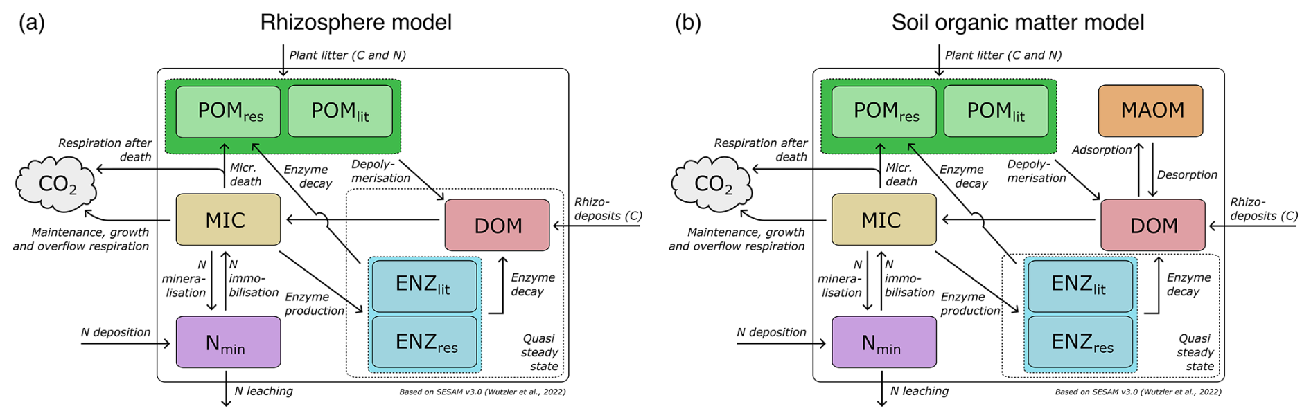
Figure 1 Illustration of (a) the rhizosphere model and (b) the soil organic matter (SOM) model. The rhizosphere model is the same as the SOM model, but without the simulation of the MAOM pool. In the rhizosphere model the size of the DOM pool is not tracked, while this is done for the SOM model. The rhizosphere model is the SESAM v3.0 model (Wutzler et al., 2022). The abbreviations are as follows: POM_res and POM_lit are particulate organic matter consisting of microbial residues and deactivated enzymes, and plant litter, respectively, MIC is microbial biomass C and N, N_min is mineral N, ENZ_res and ENZ_lit are enzymes mediating the depolymerisation of microbial residues and plant litter, respectively, DOM is dissolved organic matter (C and N), and MAOM is mineral-associated organic matter (C and N).

2.4 Mathematical models

2.4.1 The rhizosphere models

The amount of SOM was simulated down to 0.2 m for a unit surface area of 1 m², expressed as g C m⁻² or g N m⁻². The differential equations were solved using the ode solver from the deSolve package in R (Soetaert et al., 2010) with a time step of 1 d. Simulations were performed for a time span over which the model pools were shown to have reached steady state, being 500 years for the rhizosphere models, and 2000 years for the SOM model. The equations describing C and N transformations are identical to the SESAM v3.0 model, of which a detailed description can be found in Wutzler et al. (2022). Annual total OC inputs were calibrated for the SOM model to obtain a correct combination of the size of the combined POC pools and its turnover rate. This was done by optimising the value for OC inputs together with the other model parameters of the SOM model using a frequentist calibration approach (Sect. 2.5). This resulted in OC inputs of 349 $\mathrm{g}\mathrm{C}{\mathrm{m}}^{-\mathrm{2}}{\mathrm{yr}}^{-\mathrm{1}}$ (Table S8 in the Supplement), of which 80 % was assumed to enter the soil as plant litter, and the remaining 20 % as rhizodeposits. The difficulty in correctly estimating this parameter in field situations (e.g., Hirte et al., 2018; Pausch and Kuzyakov, 2018) and resulting effect on SOC model simulations (Keel et al., 2017; Taghizadeh-Toosi et al., 2016) therefore means that its uncertainty generally leads to an additional potential cause for equifinality on top of the uncertainty of model parameters necessary to calculate fluxes of OC between model pools. For example, if another value for OC inputs was obtained, the value of parameters governing OC losses would likely have been different after optimisation. We have, however, chosen not to assess this additional uncertainty to limit the complexity of the presented results. Organic N enters the soil through plant litter, assuming a constant C:N ratio of 30, while rhizodeposits are assumed to only contain C. Mineral N is added to the soil through atmospheric N deposition (0.7 $\mathrm{g}\mathrm{N}{\mathrm{m}}^{-\mathrm{2}}{\mathrm{yr}}^{-\mathrm{1}}$).

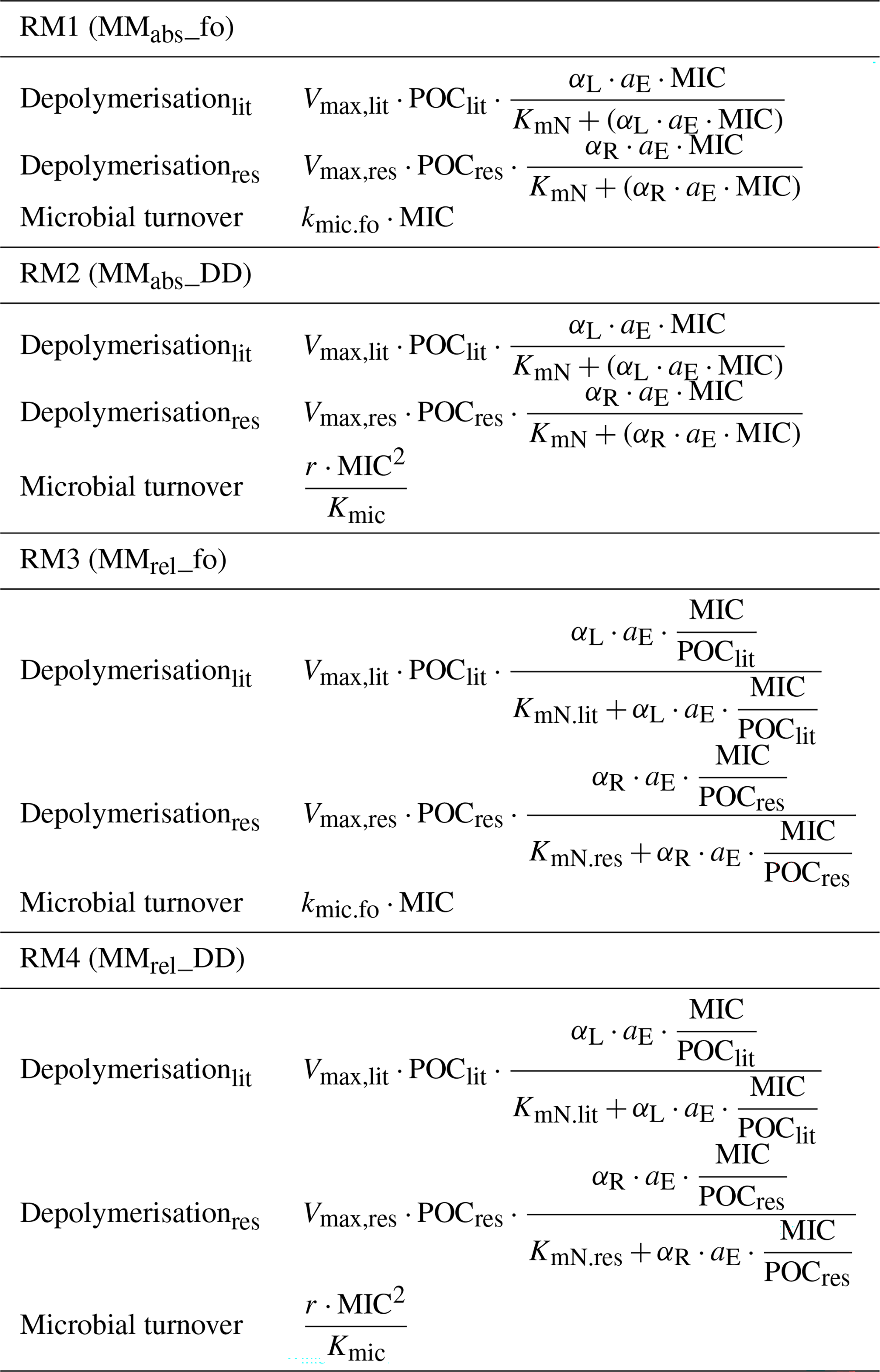
For the rhizosphere models, an overview of the state variables and parameters is presented in Tables S1 and S2 in the Supplement, respectively. Four different sets of equations were used to assess how different mathematical formulations of the same conceptual model influence parameter identifiability and consequently the consistency in model predictions. These combined either one of two variations of (1) the Michaelis–Menten equations for depolymerisation of litter (POM_lit and POM_res) and (2) microbial turnover (Table 1). The two variations for the depolymerisation of POM are referred to as the absolute and relative variants. The absolute variant is formulated as:

$$\begin{array}{}\text{(1)}& {\displaystyle }& {\displaystyle }\begin{array}{rl}{\displaystyle }& {\displaystyle }{\text{Depolymerisation}}_{\text{lit}}=\\ {\displaystyle }& {\displaystyle }{V}_{\text{max,lit}}\cdot {\text{POC}}_{\text{lit}}\cdot {\displaystyle \frac{{\mathit{\alpha }}_{\mathrm{L}}\cdot a_{\mathrm{E}}\cdot \text{MIC}}{K_{\text{mN}}+({\mathit{\alpha }}_{\mathrm{L}}\cdot a_{\mathrm{E}}\cdot \text{MIC})}}\end{array}\text{(2)}& {\displaystyle }& {\displaystyle }\begin{array}{rl}{\displaystyle }& {\displaystyle }{\text{Depolymerisation}}_{\text{res}}=\\ {\displaystyle }& {\displaystyle }{V}_{\text{max,res}}\cdot {\text{POC}}_{\text{res}}\cdot {\displaystyle \frac{{\mathit{\alpha }}_{\mathrm{R}}\cdot a_{\mathrm{E}}\cdot \text{MIC}}{K_{\text{mN}}+({\mathit{\alpha }}_{\mathrm{R}}\cdot a_{\mathrm{E}}\cdot \text{MIC})}}\end{array}\end{array}$$

Where V_max,lit and V_max,res are the maximum rates of depolymerisation of POC_lit and POC_res per time step (1 d), respectively, K_mN is the half-saturation constant (g C m⁻³), α_L and α_R are the proportions of total microbial investment in enzymes to depolymerise litter and residues (unitless, both values add up to 1), respectively, a_E the portion of microbial biomass invested in total enzyme production (unitless), and MIC is OC in the microbial biomass pool (g C m⁻²). These formulations, referred to as reverse Michaelis–Menten kinetics (Schimel and Weintraub, 2003), are identical to the original SESAM v3.0 model, and imply that the amount of depolymerisation per time step is limited by the absolute amount of extracellular enzymes. Therefore, these equations are referred to here as absolute Michaelis–Menten (MM_abs). They have been used in, among others, the COMISSION model (Ahrens et al., 2015, 2020), MIMICS (Wieder et al., 2015), and Millennial v2 (Abramoff et al., 2022), and have been shown to be the preferred formulation to represent depolymerisation of POM, compared to forward Michaelis–Menten kinetics (Tang and Riley, 2019).

In the second variant of these equations, the rate modifier is based on ratios of model pools. These are formulated as:

$$\begin{array}{}\text{(3)}& {\displaystyle }& {\displaystyle }\begin{array}{rl}{\displaystyle }& {\displaystyle }{\text{Depolymerisation}}_{\text{lit}}=\\ {\displaystyle }& {\displaystyle }{V}_{\text{max,lit}}\cdot {\text{POC}}_{\text{lit}}\cdot {\displaystyle \frac{{\mathit{\alpha }}_{\mathrm{L}}\cdot a_{\mathrm{E}}\cdot \frac{\text{MIC}}{{\text{POM}}_{\text{lit}}}}{K_{\text{mN.lit}}+{\mathit{\alpha }}_{\mathrm{L}}\cdot a_{\mathrm{E}}\cdot \frac{\text{MIC}}{{\text{POC}}_{\text{lit}}}}}\end{array}\text{(4)}& {\displaystyle }& {\displaystyle }\begin{array}{rl}{\displaystyle }& {\displaystyle }{\text{Depolymerisation}}_{\text{res}}=\\ {\displaystyle }& {\displaystyle }{V}_{\text{max,res}}\cdot {\text{POC}}_{\text{res}}\cdot {\displaystyle \frac{{\mathit{\alpha }}_{\mathrm{R}}\cdot a_{\mathrm{E}}\cdot \frac{\text{MIC}}{{\text{POM}}_{\text{res}}}}{K_{\text{mN.res}}+{\mathit{\alpha }}_{\mathrm{R}}\cdot a_{\mathrm{E}}\cdot \frac{\text{MIC}}{{\text{POC}}_{\text{res}}}}}\end{array}\end{array}$$

Where K_mN.lit is the half-saturation constant for depolymerisation of POM_lit (unitless, equivalent to the ratio of enzymes (${\mathit{\alpha }}_{\mathrm{L}}\cdot a_{\mathrm{E}}\cdot \text{MIC}$) to POM_lit), and K_mN.res being the half-saturation constant for depolymerisation of POM_res (unitless, equivalent to the ratio of enzymes (${\mathit{\alpha }}_{\mathrm{R}}\cdot a_{\mathrm{E}}\cdot \text{MIC}$) to POM_res). The rate of depolymerisation (i.e., the portion of POM depolymerised per time step) is thus limited by the ratio of MIC to POM, rather than by the absolute amount of MIC. Therefore, these formulations are referred to as relative Michaelis–Menten (MM_rel), and imply that the more microbes (and thus extracellular enzymes) are available per unit of POM, the larger the portion of POM that will be depolymerised. Similar formulations have been used in CORPSE-N (Sulman et al., 2019), AMPSOM (Tougma et al., 2025) and SOILcarb (Van de Broek et al., 2025).

Two different approaches to simulate microbial turnover were tested: first-order decay (fo) and density-dependent turnover (DD). First-order microbial turnover per time step is simulated as:

$$\begin{array}{}\text{(5)}& \text{Mortality}=k_{\text{mic.fo}}\cdot \text{MIC}\end{array}$$

Where k_mic.fo is the portion of microbes turning over per time step (d⁻¹). This formulation is common in microbially-driven SOC models (e.g., Allison et al., 2010; Riley et al., 2014; Woolf and Lehmann, 2019; Yu et al., 2020; Laub et al., 2024). Density-dependent microbial turnover (Buchkowski et al., 2017) is formulated using a logistic growth model (the Verhulst equation or Verhulst-Pearl equation) expressing the rate of change in microbial biomass per unit of time:

$$\begin{array}{}\text{(6)}& {\displaystyle \frac{\mathrm{d}\text{MIC}}{\mathrm{d}t}}=r\cdot \text{MIC}\times \left(\mathrm{1}-{\displaystyle \frac{\text{MIC}}{K_{\text{mic}}}}\right)\end{array}$$

Where MIC is the microbial biomass (g C m⁻²), t the time (d), r the growth rate (d⁻¹) and K_mic the carrying capacity for MIC (g C m⁻²). The latter is expressed as a portion (f_K) of total POC (the sum of POC_lit and POC_res). Equation (6) can then be reformulated as:

$$\begin{array}{}\text{(7)}& {\displaystyle \frac{\mathrm{d}\text{MIC}}{\mathrm{d}t}}=r\cdot \text{MIC}-{\displaystyle \frac{r\cdot {\text{MIC}}^{\mathrm{2}}}{f_{\mathrm{K}}\cdot ({\text{POC}}_{\text{lit}}+{\text{POC}}_{\text{res}})}}\end{array}$$

This formulation is equivalent to the formulation of density-dependent microbial turnover in Georgiou et al. (2017), and shows that the loss of microbial biomass per unit of time (second term on the right-hand side) is a function of the square of microbial biomass. The use of this equation implies that the carrying capacity of microbial biomass (K_mic) needs to be known or calibrated, instead of the explicit turnover rate. Similar formulations have been shown to lead to less severe oscillations in simulated SOC stocks over time (Georgiou et al., 2017), and have been implemented in, for example, the versions of ReSOM (Tang and Riley, 2015) used in Sulman et al. (2018) and Van de Broek et al. (2024). The combinations of both approaches to simulate depolymerisation and uptake, on the one hand, and microbial turnover, on the other hand, led to four different formulations of the rhizosphere model (Table 1).

Table 1 Overview of the equations used in the four rhizosphere models (RM). MM_abs and MM_rel refer to absolute and relative Michaelis–Menten kinetics, respectively, fo and DD refer to first-order and density-dependent microbial mortality, respectively. The parameters are explained in Table S2.

2.4.2 The soil organic matter model

The inputs of C and N in the SOM model were equal to the inputs simulated in the rhizosphere models. The equations for the SOM model were chosen from the rhizosphere model with relative Michaelis–Menten depolymerisation and density-dependent microbial turnover (RM4, see Sect. 2.4.1). An overview of the state variables and parameters of the SOM model is presented in Table S3 and S4 in the Supplement, respectively. Depolymerisation of POM_lit and POM_res are simulated using Eqs. (3) and (4), respectively, and the mortality of microbes as the last term on the right-hand side of Eq. (7).

Competition for DOM between microbes (for uptake) and soil minerals (for adsorption) is simulated using the equilibrium chemistry approximation (ECA;  Tang and Riley, 2013). This approach partitions a substrate between two enzymes using the affinity of both enzymes for the substrate. Because not all substrate is partitioned between the sinks in a single time step, the DOM pool was explicitly simulated to keep track of its size, in contrast to the rhizosphere models and the original SESAM v3.0 model. The implementation of ECA kinetics follows Tang and Riley (2013):

$$\begin{array}{}\text{(8)}& {\displaystyle }& {\displaystyle }\begin{array}{rl}{\displaystyle }& {\displaystyle }{\text{Uptake}}_{\text{ECA}}=\\ {\displaystyle }& {\displaystyle }\text{MIC}{\displaystyle \frac{\text{DOM}}{K_{\text{m,U}}\left(\mathrm{1}+\frac{{\text{SURF}}_{\text{rhizo}}}{K_{\text{m,ads}}}+\frac{\text{MIC}}{K_{\text{m,U}}}\right)+\text{DOM}}}\end{array}\text{(9)}& {\displaystyle }& {\displaystyle }\begin{array}{rl}{\displaystyle }& {\displaystyle }{\text{Adsorption}}_{\text{ECA}}=\\ {\displaystyle }& {\displaystyle }{\text{SURF}}_{\text{rhizo}}{\displaystyle \frac{\text{DOM}}{K_{\text{m,ads}}\left(\mathrm{1}+\frac{{\text{SURF}}_{\text{rhizo}}}{K_{\text{m,ads}}}+\frac{\text{MIC}}{K_{\text{m,U}}}\right)+\text{DOM}}}\end{array}\end{array}$$

Where K_m,U is the affinity constant for microbial uptake of DOM (g C m⁻³), K_m,ads the affinity constant for OM adsorption (g C m⁻³), and SURF_rhizo the amount of available surfaces for OM adsorption in the rhizosphere (g C m⁻³). The latter was calculated by subtracting the simulated amount of MAOC from the SOC stabilisation potential calculated using the clay+silt content (assumed to be 50 %) following Georgiou et al. (2022), and multiplying this value with the volume of the rhizosphere to account for the fact that not all soil minerals are in touch with inputs of C and N from roots. This was assumed to be 10 % of total soil volume (based on calculations by Finzi et al., 2015) at the initiation of the simulation. After the simulated OC inputs were doubled (see Sect. 2.8), also SURF_rhizo was doubled, assuming OC inputs increase proportional to root biomass.

Desorption of OM from minerals was simulated as a first-order process:

$$\begin{array}{}\text{(10)}& \text{Desorption}=k_{\text{des}}\cdot \text{MAOM}\end{array}$$

With k_des being the desorption rate (d⁻¹).

2.4.3 Simulation of Δ¹⁴C

For the SOM model, the Δ¹⁴C value of SOC was simulated to evaluate how including data on the Δ¹⁴C values of measurable model pools (i.e., POC and MAOC) affects the identifiability of model parameters. The dataset for the annual Δ¹⁴C value of atmospheric CO₂ in the northern hemisphere compiled by Van de Broek et al. (2025) (using data from Reimer et al., 2013, Hua et al., 2013 and Hammer and Levin, 2017) was used, and a lag time of 4 years between the incorporation of atmospheric ¹⁴CO₂ in plant biomass and the addition of this biomass to the SOC pool was used, following previous modelling studies (Ahrens et al., 2014; Schrumpf and Kaiser, 2015). No kinetic fractionation of ¹⁴C relative to ¹²C was assumed during the transfer of ¹⁴C between simulated pools, with radioactive decay being the only mechanism leading to additional losses of ¹⁴C compared to ¹²C. Values of Δ¹⁴C were calculated assuming the OC had a δ¹³C value of −28 ‰, and that soil samples were collected in 2007 (see Sect. 2.2).

2.5 Deterministic parameter calibration

To evaluate the sensitivity and identifiability of model parameters, it was necessary to have a set of parameter values that leads to realistic model results with the model output being sensitive to local changes in parameter values. Therefore, a deterministic calibration was performed using the differential evolution (DE) algorithm (Storn and Price, 1997) as implemented in the DEoptim package in R (Mullen et al., 2011; Ardia et al., 2011). For the rhizosphere models, between 3 and 5 parameters were optimised (depending on model variant, Table S5 in the Supplement), while for the SOM model, 9 parameters were optimised (Table S6 in the Supplement). The parameter values were optimised by minimising the sum of squared relative errors (SSRE), formulated as:

$$\begin{array}{}\text{(11)}& \text{SSRE}=\sum _{i=\mathrm{1}}^n{\left({\displaystyle \frac{{\text{meas}}_i-{\text{mod}}_i}{{\text{meas}}_i}}\right)}^{\mathrm{2}}\end{array}$$

Where n is the number of measurements, and meas_i and mod_i are the measured and modelled pool sizes, respectively.

For the rhizosphere models, artificial measurements of POC, MIC and the C:N ratio of total SOM were used to optimise model parameters with a population size of 180 parameter sets for 500 iterations. To make sure that the rate modifiers of the Michaelis–Menten equations for depolymerisation of microbial residues and litter were sensitive to changes in the size of model pools, their artificial measured value was assumed to be 0.5, and the SSRE calculated accordingly. For the rhizosphere model with first-order microbial mortality, the decay constant (k_mic.fo) was kept constant at a value of 0.01 d⁻¹, to simulate a turnover rate of the microbial biomass of 100 d. For the rhizosphere models with density-dependent microbial turnover, the turnover rate of microbes was calibrated to be as close as possible to 100 d. The optimised parameter values for the rhizosphere models are shown in Table S7 in the Supplement.

For the SOM model, artificial measurements of POC, MAOC, total OC, the C:N values of POM and MAOM, and the Δ¹⁴C values of POC and MAOC were used to optimise model parameters with a population size of 180 parameter sets for 500 iterations. Similar to the rhizosphere model, the rate modifiers for the Michaelis–Menten equations simulating depolymerisation of litter and microbial residues were optimised to be as close to 0.5 as possible. The turnover rate of microbes was calibrated to be as close as possible to 100 d. The optimised parameter values for the SOM model are shown in Table S8.

2.6 Parameter identifiability analysis

To assess which parameter combinations were identifiable, given different available data sets for parameter optimisation, the methods developed by Brun et al. (2001) were applied using the FME package in R (Soetaert and Petzoldt, 2010). For the rhizosphere models, three scenarios of data availability were tested: (1) only data on total SOC, (2) data on total SOC and total N, and (3) data on POC, MIC and the C:N ratio of total SOC. The first scenario is one with a minimum data availability, while the second scenario is considered the most common (as C and N are often measured together). The third scenario assumes that in addition to total C and N, also microbial biomass C and POC were measured. Also for the SOM model, three scenarios of data availability were tested: (1) data on total SOC and N, (2) data on POC, MAOC and their C:N ratios, and (3) data on POC, MAOC, their C:N ratios, and the Δ¹⁴C values of POC and MAOC. The choice of these scenarios was based on common practices in SOM modelling, although data availability may be more extensive in other studies. As the identifiability analysis needs to be performed with a parameter set that leads to an acceptable model output (Brun et al., 2001), the identifiability analysis was performed using the optimal parameter set obtained from the deterministic DE calibration (see Sect. 2.5).

To perform the identifiability analysis, the local sensitivity of selected model state variables to variations in parameter values was quantified using a normalised, dimensionless sensitivity index (Brun et al., 2001):

$$\begin{array}{}\text{(12)}& s_{ij}={\displaystyle \frac{\partial y_i}{\partial {\mathrm{\Theta }}_j}}{\displaystyle \frac{w_{{\mathrm{\Theta }}_j}}{w_{y_i}}}\end{array}$$

Where y_i is the ith state variable, Θ_j is the jth model parameter, $w_{{\mathrm{\Theta }}_j}$ is a weighting factor for Θ_j,and $w_{y_i}$ is a weighting factor for y_i. The obtained sensitivity matrix (s) thus quantifies the rate of change in the value of model output y_i for a small change in the value of parameter Θ_j. The weighting factor for the parameter value ($w_{{\mathrm{\Theta }}_j}$) was set to the optimal parameter value obtained by the DE optimisation, while the weighting factor for the state variable ($w_{y_i}$) is the steady-state size of this pool obtained using the optimal parameter values from the DE optimisation. The weights were thus constant for every assessed combination of state variable and parameter.

This local sensitivity analysis as implemented in the FME package in R (Soetaert and Petzoldt, 2010) evaluates the sensitivity for a time series of model outputs and respective measurements. As we assumed to only have steady-state measurements at one point in time, the sensitivity of the model output could only be evaluated for this one time point. To do so, the sensitivity analysis from the FME package was run multiple times, each iteration changing the parameter values with a different relative amount (from $\mathrm{1}\times {\mathrm{10}}^{-\mathrm{4}}-\mathrm{5}\times {\mathrm{10}}^{-\mathrm{4}}$ in steps of $\mathrm{5}\times {\mathrm{10}}^{-\mathrm{5}}$). These results were then combined to construct the sensitivity matrix (Eq. 12), with rows containing the sensitivity indexes (s_ij) quantifying how varying parameters by a different relative amount affected the selected model output, and columns showing this for different parameters. One alteration made to the sensitivity analysis from the FME package (in the function sensFun) is that the tested parameter values were not restricted to be larger than the relative deviation (as was implemented by Soetaert and Petzoldt, 2010), to make sure the proposed range in parameter values was tested and not replaced by the relative deviation.

The sensitivity matrices were subsequently used to assess the parameter identifiability through the analysis of collinearity between all possible combinations of columns (i.e., parameters). As every column quantifies how every evaluated model state variable changes when a parameter value is altered, columns having a high collinearity indicate parameter combinations that are not identifiable, as a change in one parameter can be compensated by a change in one or more other model parameters. Before the collinearity was assessed, every column in the sensitivity matrix was normalised using the Euclidean norm (i.e., the square root of the sum of the squared values), following Brun et al. (2001):

$$\begin{array}{}\text{(13)}& \widehat{{\mathit{s}}_j}={\displaystyle \frac{{\mathit{s}}_j}{\Vert {\mathit{s}}_j\Vert }}\end{array}$$

Where $\widehat{{\mathit{s}}_j}$ is the normalised column for the jth parameter in s_ij, s_j is the original column, and $\Vert {\mathit{s}}_j\Vert$ is the Euclidean norm of column s_j. Combining these columns for all parameters results in the normalised sensitivity matrix $\widehat{\mathbf{S}}$. For every combination of columns (i.e., parameters) in $\widehat{\mathbf{S}}$, a collinearity index was calculated (Brun et al., 2001):

$$\begin{array}{}\text{(14)}& \mathit{\gamma }={\displaystyle \frac{\mathrm{1}}{\sqrt{min\left(\text{EV}\right[{\widehat{S}}^{\mathrm{T}}\widehat{S}\left]\right)}}}\end{array}$$

Where γ is the collinearity index, ${\widehat{\mathit{S}}}^{\mathrm{T}}\widehat{\mathbf{S}}$ is the vector product of $\widehat{\mathbf{S}}$ and the transposed vector $\widehat{\mathbf{S}}$, and min(EV) is the smallest eigenvalue of this product. The interpretation of γ is that a change in one parameter can be compensated by $\mathrm{1}-\mathrm{1}/\mathit{\gamma }$ when one or more parameters are appropriately changed. To label a parameter set as being identifiable, we used a threshold of γ of 10, meaning that a parameter change can be undone for 90 % by changes in other parameter values. It is noted that various studies have used different values for this threshold, generally in the range $\mathrm{5}<\mathit{\gamma }<\mathrm{20}$ (Brun et al., 2001). A detailed description of the methods presented in this section is provided in Brun et al. (2001), and examples of its application are shown in, among others, Omlin et al. (2001), Brun et al. (2002) and Sierra et al. (2015).

2.7 Bayesian parameter calibration

Parameter optimisation was performed to obtain as many parameter combinations as possible that produce behavioural models, i.e., model outputs that cannot readily be rejected given available data. These are defined here as predictions within one standard deviation of the measurements. To account for measurement uncertainty, a Bayesian calibration was performed using the Differential Evolution Markov Chain with snooker updater (DEzs) algorithm (ter Braak and Vrugt, 2008), as implemented in the BayesianTools package in R (Hartig et al., 2023). As no prior information on the distribution of parameter values was known, uniform priors were used within specified bounds (see Table S6) and the log-likelihood was calculated as (Vrugt, 2016):

$$\begin{array}{}\text{(15)}& \begin{array}{rl}{\displaystyle }\mathcal{L}\left(\mathit{x}\right|\stackrel{\mathrm{̃}}{\mathbf{Y}},{\widehat{\mathit{\sigma }}}^{\mathrm{2}})=& {\displaystyle }-{\displaystyle \frac{n}{\mathrm{2}}}\log \left(\mathrm{2}\mathit{\pi }\right)-{\sum }_{i=\mathrm{1}}^n\log \left(\widehat{{\mathit{\sigma }}_i}\right)\\ {\displaystyle }& {\displaystyle }-{\displaystyle \frac{\mathrm{1}}{\mathrm{2}}}{\sum }_{i=\mathrm{1}}^n{\left({\displaystyle \frac{\stackrel{\mathrm{̃}}{y_i}-y_i\left(\mathit{x}\right)}{\widehat{{\mathit{\sigma }}_i}}}\right)}^{\mathrm{2}}\end{array}\end{array}$$

Where n is the number of observations, $\widehat{{\mathit{\sigma }}_i}$ is the standard deviation of the ith observation, $\stackrel{\mathrm{̃}}{y_i}$ is the ith observation, and y_i(x) is the model prediction of this observation.

For the rhizosphere models, the DE_zs algorithm was run using 5 internal chains, higher than the three internal chains which have been shown to be sufficient to explore a high dimensional parameter space (ter Braak and Vrugt, 2008). This was done 3 times (i.e., with three independent chains), to ensure an optimal exploration of the parameter space. Each internal chain was run for 20 000 iterations. The Bayesian calibrations of the SOM model were run with a number of internal chains equal to twice the number of optimised parameters (Table 2) with 20 000 iterations each, repeated 3 times to obtain 3 independent chains. For these calibrations, the chance of a snooker jump was increased to 0.2 (from the default 0.1), to enhance exploration of the parameter space and avoid the algorithm getting stuck in a local maximum.

The four rhizosphere models were used to illustrate the concept of parameter identifiability and the consequences of equifinality on model predictions. To do so, each of the rhizosphere models was calibrated twice. In a first scenario (termed the full parameter model; FPM) all parameters for which no realistic estimates could be made or found in the literature were optimised (either 5 or 6 parameters, depending on the model; Table S9 in the Supplement). These parameter sets were non-identifiable. In a second scenario (termed the identifiable parameter model; IPM), only identifiable parameters for the assumed data were optimised: V_max,lit and V_max,res (see Tables S11, S13, S15 and S17 in the Supplement). These parameters were identified using the parameter identifiability analysis for each model separately (Sect. 2.6). In addition to these parameter values, also the rate modifiers for the depolymerisation of POM_lit and POM_res (see Eq. 1 and 2) were optimised to be as close as possible to 0.5. For both optimisation scenarios, it was assumed that only measurements of total SOC and the C:N ratio were available, as these data are most commonly available. The values of the parameters that were not optimised were fixed at the values obtained through the deterministic calibration (Sect. 2.5). This means there is an additional hidden uncertainty, as the values of the fixed parameters could not be confidently determined, while choosing different values would likely have led to other calibrated values for the optimised identifiable parameters. This uncertainty is, however, not assessed in the present study.

For the SOM model, Bayesian parameter optimisation was performed for three assumptions on data availability: (1) data on total SOC and N (referred to as OM_tot), (2) data on POC, MAOC, particulate N and mineral-associated N (which can be obtained through SOM fractionation, referred to as Fractions), and (3) data on POC, MAOC, particulate N, mineral-associated N and the Δ¹⁴C values of POC and MAOC (referred to as Fractions and Δ¹⁴C). For each of these data sets, one full parameter model (FPM) was run by optimising eight parameters for which no reasonable estimate could be made (Table 2), and one identifiable parameter model (IPM), optimising as many parameters as could be jointly identified: 2 for the OM_tot scenario, 3 for the Fractions scenario, and 5 for the Fractions and Δ¹⁴C scenario (Table 2).

Table 2 Optimised identifiable parameters during the Bayesian calibration of the identifiable parameter model (IPM) version of the soil organic matter (SOM) model for the three scenarios: OM_tot (calibration using only data on total organic carbon (OC) and N), Fractions (calibration based on the OC and N content of particulate (POM) and mineral-associated organic matter (MAOM)) and Fractions and Δ¹⁴C (calibration based on the OC and N content and Δ¹⁴C values of POM and MAOM). The columns show all parameters that were selected as requiring optimisation in the full parameter model (FPM). Information about the parameters is presented in Table S4.

2.8 Disturbing the steady state solution

All results obtained by the Bayesian calibration were within one standard deviation from the average respective measurements (behavioural models). This implies that none of these models (and their parameter sets) could readily be rejected given the variability in measurements. To assess how different sets of optimised parameter combinations, i.e., identifiable versus non-identifiable, affect model predictions starting from steady-state pool sizes, OC inputs were doubled for a period of 100 years. Subsequently, the amount of simulated total SOC of the simulated pools was analysed after 100 years. The additional uncertainty caused by parameter equifinality was assessed for the different scenarios by quantifying the absolute value and spread of model predictions upon the doubling of OC inputs.

3 Results

3.1 Rhizosphere models

3.1.1 Parameter identifiability

The parameter identifiability analysis for all four rhizosphere models showed that the number of identifiable parameters was limited, and increased when more data were available for parameter optimisation (Fig. 2 and Tables S11–S18 in the Supplement). When only total OC data were available, none of the four models had two parameters that could be simultaneously identified. For the scenario where data on both total OC and N was available, maximum two parameters could be identified together. Three parameters were jointly identifiable only when total OC, N and microbial biomass data were present. This shows that even for models developed with trade-offs between model complexity and data availability in mind (Wutzler et al., 2022), the number of parameters that can be optimised without overparameterisation is well below the total number of unknown model parameters (five or six, depending on the model formulation; Table S9).

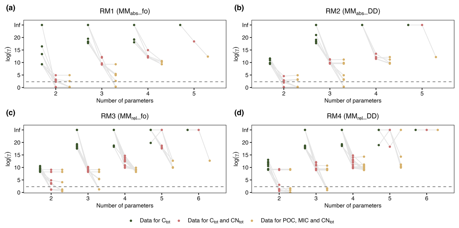
Figure 2 Logarithm of the collinearity index (γ) for all parameter combinations of the four rhizosphere models, for the scenarios where (1) only data on total SOC were available (green dots), (2) data total SOC and N were available (red dots) and (3) data on total SOC, N and microbial biomass C were available (yellow dots). The same parameter combinations are connected by grey lines. The dotted horizontal line shows the threshold in γ (log (10)=2.3) below which parameter combinations are considered to be identifiable. Infinite values (Inf) of γ indicate that the columns of the sensitivity matrix are linearly dependent, meaning that parameter values perfectly compensate for each other. The identifiable parameter combinations are shown in Tables S11–S18.

3.1.2 The effect of overparameterisation on equifinality in rhizosphere model predictions

Disturbing the steady-state solution of the rhizosphere models by forcing a doubling of OC inputs revealed the difference in model evaluation between steady-state simulations and predictions made with the same models. The Bayesian optimisation of all rhizosphere models to steady state (the simulations at year 500 in Fig. 3) successfully produced behavioural models of which the simulation of total OC fell within the measurement uncertainty range. If no further simulations were performed, all these model outcomes would therefore have been considered highly accurate and precise. However, predictions differed between the models when OC inputs were doubled.

Predictions by the identifiable parameter models showed that RM1 and RM2, with absolute Michaelis–Menten kinetics, predicted a lower average relative increase in OC (61.1 %–70.7 %; Fig. 3c and f) compared to RM3 and RM4, with relative Michaelis–Menten kinetics (100 %; Fig. 3i and l). This difference is due to the formulation of the rate modifiers for depolymerisation (Table 1). For RM1 and RM2, the simulated fraction of POC being depolymerised is determined by the absolute size of the microbial pool, which doubled upon a doubling of OC inputs for RM1 and increased by 67.2 %–70.7 % for RM2 (Fig. S1a and d in the Supplement). This caused an increase in the rate modifier for depolymerisation of POC_lit upon a doubling of OC inputs (Fig. S1b and e), leading to a higher fraction of POC_lit being depolymerised compared to under the initial OC inputs. This is also reflected in a decrease in the turnover time of POC after C inputs are doubled, resulting from the faster turnover (Fig. S1c and f). In contrast, the pools controlling the value of the rate modifier for POC_lit in RM3 and RM4 (the ratio of MIC to POC_lit) remained constant upon a doubling of OC inputs, causing the rate modifier to be identical before and after a doubling of OC inputs (Fig. S1g, h, j, and k). As a result, the same fraction of POC_lit was depolymerised per time step upon a doubling of OC inputs, as is also evidenced by the lack of a change in the turnover rates of POC after OC inputs were doubled (Fig. S1i and l). This difference shows the effect of mathematical formulations on model predictions, using either absolute or relative Michaelis–Menten rate modifiers.

Also the number of optimised parameters had an effect on predictions by the rhizosphere models. For RM1 and RM2 (with absolute Michaelis–Menten kinetics), the average relative increase in OC upon a doubling of inputs was lower for the full parameter models than for the identifiable parameter models (Fig. 3c and f). In contrast, for RM3 and RM4 (with relative Michaelis–Menten kinetics), overparameterisation did not affect the average increase in OC, which was ca. 100 %. Moreover, the range in predictions was ca. 42 times larger for RM1 for the full parameter models (a range of 34 %, i.e., between 34.5 % and 68.5 %, Fig. 3c) compared to the identifiable parameter models (a range of 0.8 %, i.e., between 61.1 % and 61.9 %, Fig. 3c). For RM2, the range in predictions was ca. 6 times larger for the full parameter models (a range of 21.2 %, i.e., between 54 % and 75.2 %, Fig. 3f) compared to the identifiable parameter models (a range of 3.5 %, i.e., between 67.2 % and 70.7 %, Fig. 3f). These results show that the accurate prediction of steady-state stocks of SOC by behavioural models is not a sufficient criterion to evaluate the predictive capabilities of such models.

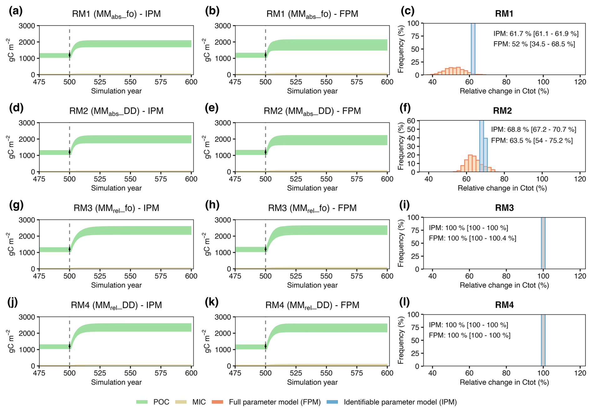
Figure 3 The effect of parameter identifiability and resulting equifinality on the prediction of SOC by the four rhizosphere models (RMs). Each row shows the results for a different model (see Table 1). The first column shows the results from a Bayesian optimisation of two identifiable parameters (the Identifiable Parameter Model: IPM), while the second column shows the results from a Bayesian optimisation of five (RM1 and RM2) or six (RM3 and RM4) parameters (the Full Parameter Model: FPM). Note that the lines for total SOC are not shown, as these overlapped with POC. The evolution of the MIC pool for the IPM models is enlarged in Fig. S1. The last column shows frequency diagrams of the relative increase in SOC after a doubling of OC inputs after simulation year 500 (as shown by the vertical dashed line). The text reports the median increase, with the range between square brackets. The black dots show the average OC measurement in simulation year 500, and vertical black bars show the standard deviation.

3.2 Soil organic matter model

3.2.1 Parameter identifiability

The parameter identifiability analysis for the SOM model showed that, similar to the results for the rhizosphere models, the number of identifiable parameters increased with an increasing quantity of calibration data (Fig. 4). When only data on total SOC and N were used, at most two parameters were jointly identifiable, while three parameters were identifiable together when data on the fractions of POC, MAOC and their N content were used. The number of identifiable parameters increased to five when, in addition to C and N data on the POM and MAOM fractions, also the Δ¹⁴C values of these pools were used. Also here, this analysis shows that even for the scenario with the most data, not all model parameters were identifiable.

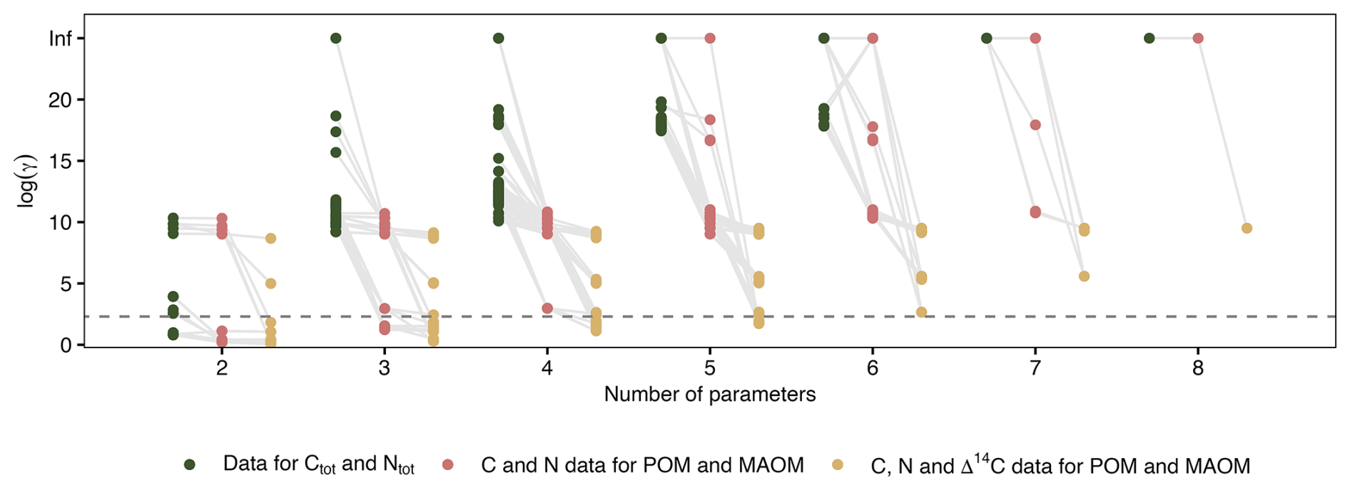
Figure 4 Logarithm of the collinearity index (γ) for all parameter combinations of the SOM model, for the scenarios where (1) only data on total SOC and N were used as calibration constraints (green dots), (2) data on the OC and N content of the POM and MAOM fractions were used (red dots), and (3) data on the OC and N content and Δ¹⁴C values of the POM and MAOM fractions were used (yellow dots). The same parameter combinations are connected by grey lines. The dotted horizontal line shows the threshold in γ (log (10)=2.3) below which parameter combinations were considered to be identifiable. Infinite values (Inf) of γ indicate that the columns of the sensitivity matrix are linearly dependent, meaning that parameter values perfectly compensate for each other. The identifiable parameter combinations are shown in Tables S19–S21 in the Supplement.

3.2.2 The effect of overparameterisation and equifinality on steady-state models

The Bayesian parameter optimisations for the SOM model resulted in behavioural models for all calibration scenarios, as total SOC was predicted to be within one standard deviation of the average measurement at steady state (Fig. 5). However, the calibration scenario had a substantial impact on the internal dynamics of the model. For example, when model parameters were optimised using only data on total SOC and N while calibrating all model parameters, the majority of SOC could be either in POC or MAOC (Fig. 5b, note that the lines for the POC pool are covered by the lines for the MAOC pool, as both pools span the entire range of potential values from a very small size to almost all SOC present in these pools; their density distribution is shown in Fig. S3 in the Supplement), demonstrating equifinality resulting from overparameterisation. Further evidence for equifinality is present when looking at the simulated Δ¹⁴C values. These are a result of the turnover rate of the respective pools, and provide a better understanding of the temporal dynamics of the model pools (Fig. 6). First, none of the scenarios lacking Δ¹⁴C data of POC and MAOC resulted in the correct simulation of the Δ¹⁴C value of these pools as measured in 2007 (Fig. 6a–d). Second, the overparameterised models (FPM) without Δ¹⁴C data being used for calibration showed large variations in the temporal trend of simulated Δ¹⁴C values of model pools (Fig. 6b and d). This shows that the simulated turnover rate of the model pools differed substantially among the behavioural models. Third, only when Δ¹⁴C data for POC and MAOC were used as a calibration constraint was the turnover time of the POC and MAOC pools correctly simulated (Fig. 6e and f).

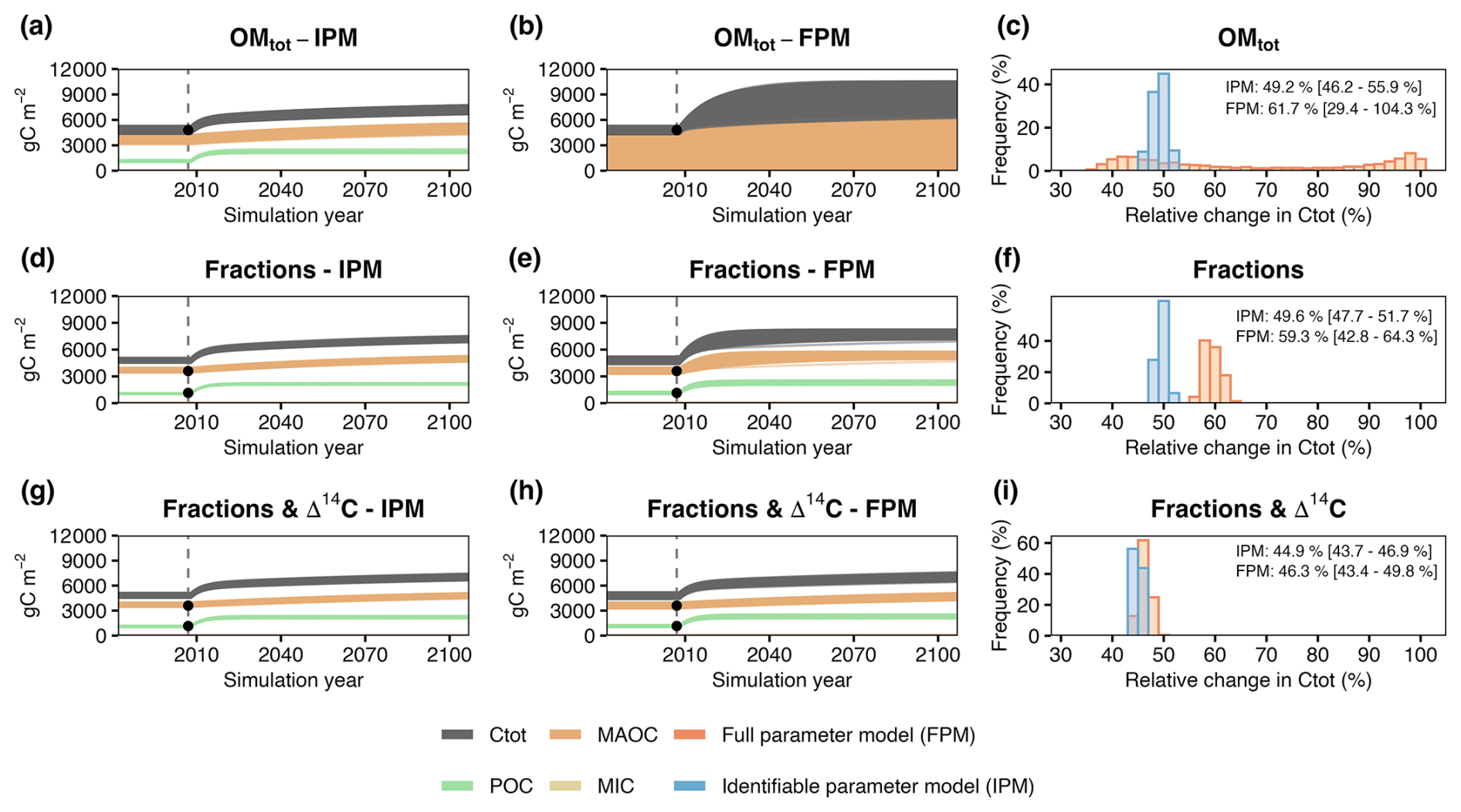
Figure 5 Results of the Bayesian calibration of the SOM model using different data constraints: (1) only total SOC and N (OM_tot; a–c), (2) the OC and N content of the POM and MAOM fractions (Fractions; d–f), and (3) the OC and N content and Δ¹⁴C values of the POC and MAOC fractions (Fractions and Δ¹⁴C; g–i). The first two columns show the simulations for the different simulated pools, with the first column showing the results for the case when only identifiable parameter sets were optimised (the identifiable parameter model: IPM), while the second column shows results for the case when a non-identifiable parameter set (i.e., all model parameters) was optimised (the full parameter model: FPM). We note that due to the small size of the MIC pool, these lines are difficult to see. The black circles show the data used for parameter optimisation, while the vertical dashed lines show the timing of the doubling of OC inputs. The corresponding simulations of Δ¹⁴C are shown in Fig. 6. The histograms on the right show the relative change in SOC for the year 2107, after a doubling of OC inputs from the year 2007 onwards. The text reports the median increase, with the range between square brackets.

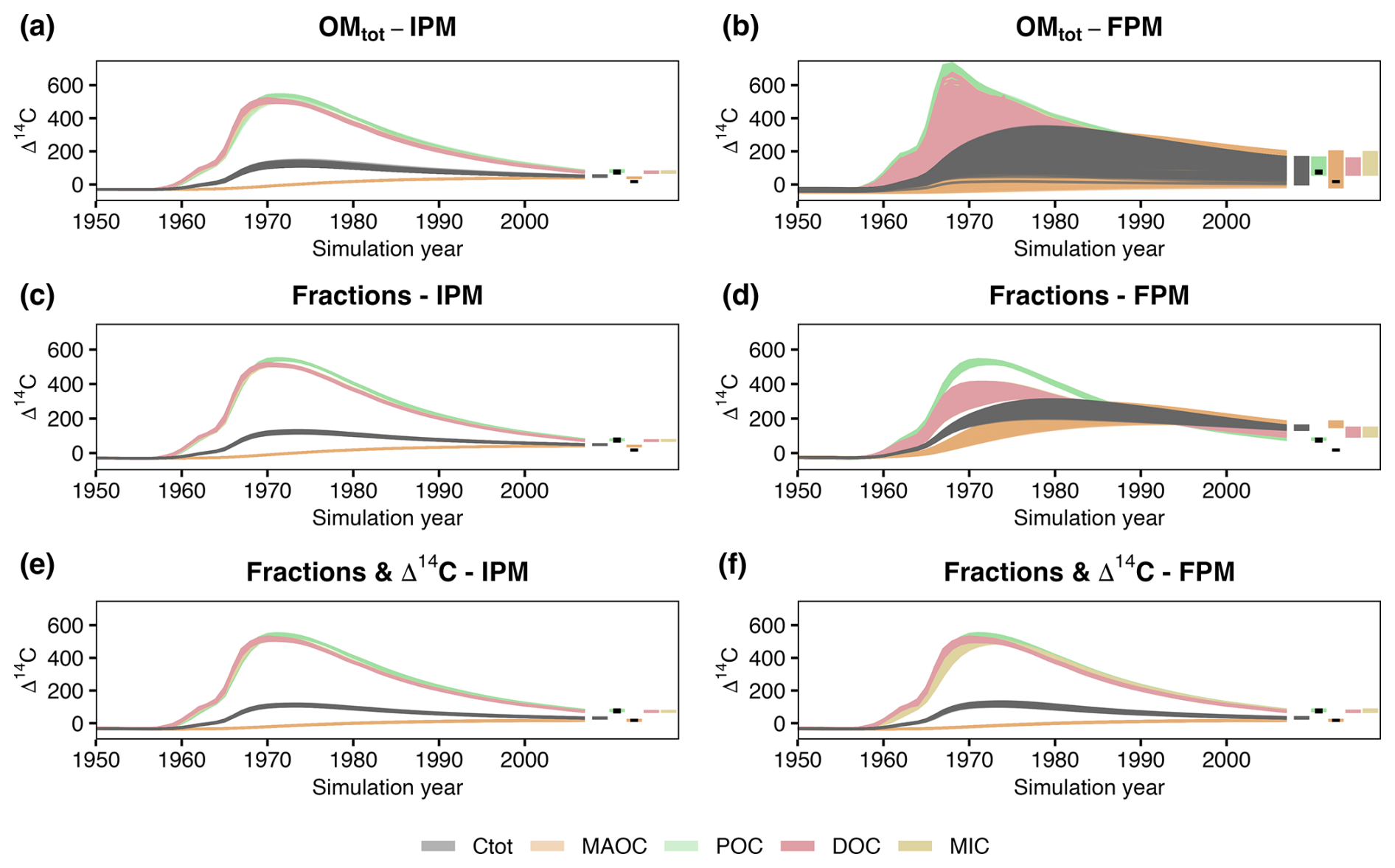
Figure 6 Simulated Δ¹⁴C values of the model pools shown in Fig. 5, for the period of the “bomb spike” in atmospheric Δ¹⁴CO₂ that occurred in the second half of the 20th century. The bars on the right of each graph show the range in simulated Δ¹⁴C in the year 2007, together with the average ± standard deviation of assumed measurements for the POC and MAOC pools in black.

Also the simulated turnover times of the microbial pool provide indications for the presence of equifinality in the behavioural models (Fig. S2 in the Supplement). These results show that for every scenario in which the carrying capacity of soil microbes was optimised (Fig. S2b, d, e and f), there was a large variation in microbial turnover time for the behavioural models, ranging from ca. 7–500 d. Furthermore, the C:N ratio of the POM and MAOM pools was better constrained in models with identifiable parameters, compared to the full parameter models (Fig. S4 in the Supplement). For the latter, the range in simulated C:N ratios of POM and MAOM was smaller when more calibration data were used. An incorrect simulation of the C:N ratio of POM and MAOM shows that the relative contribution of plant-derived (with a simulated C:N ratio of 30) and microbial-derived OC (with a simulated C:N ratio of 10) of these pools can take a range of values for the behavioural models. This is another example of the manifestation of equifinality.

3.2.3 The effect of overparameterisation and equifinality on SOM model predictions

The simulated increase in SOC stocks upon a doubling of OC inputs for the SOM model shows that overparameterisation and the resulting equifinality had a large effect on predictions (Fig. 5). All models for which only identifiable parameters were optimised (IPM) simulated a relative increase in SOC between 43.7 % and 55.9 %. In contrast, overparameterised models (FPM) simulated a larger increase in SOC stocks when no data on the Δ¹⁴C values of POC and MAOC were used as calibration constraints (Fig. 5c and f). This overestimation was greatest and least precise for the calibration scenario when only data on total SOC and N were available (an increase ranging from 29.4 %–104.3 %, with a median increase of 61.7 %), and slightly smaller when data on the OC and N content of the POC and MAOC pools was available (a median increase of 59.3 %). Only with Δ¹⁴C data for POC and MAOC were the predictions similar between the models with identifiable parameters and the full parameter model (Fig. 5i). These results underline the importance of avoiding overparameterisation to make reliable model predictions. In addition, similar to the rhizosphere models, they show that the performance of models in steady state (i.e., the behavioural models) is not a sufficient indicator for the performance when making predictions. One has to keep in mind, however, that multiple uncertain model parameters had to be fixed in the IPM models, leading to hidden uncertainty about the accuracy of the simulations.

4 Discussion

The discussion is structured around four main conclusions drawn from the results: (1) differences in the mathematical formulation of simulated processes led to different simulated changes in POM, (2) although the simulated steady-state organic matter matched measurements well (the behavioural models), this alone is insufficient to evaluate model performance under an external forcing, (3) including calibration data on internal model pools and their turnover rates reduced prediction uncertainty; and (4) optimising only identifiable model parameters similarly reduced the uncertainty of predictions, while not eliminating it due to uncertainties caused by the values of the fixed parameter values. The discussion concludes with making recommendations for incorporating parameter identifiability analysis into the model development and evaluation process.

4.1 Different model structures lead to different predictions

The simulations with the rhizosphere models showed that the choice of the mathematical formulations has a large impact on predictions. Although all model formulations led to behavioural steady-state models, the use of different equations for the depolymerisation of POM (absolute versus relative Michaelis–Menten kinetics) and microbial turnover (first-order versus density-dependent) led to different predictions in SOM upon a doubling of OC inputs (Fig. 3). A similar result was obtained by Van de Broek et al. (2024), who showed that different formulations of the thermal adaptation of soil microbes resulted in large differences in predicted losses of SOC in a soil warming experiment. While many of the recently developed mechanistic SOM models use a range of mathematical formulations (Chandel et al., 2023), the quantitative evaluation of different equations on predictions made by recently-developed models received little research attention to date. Similarly, microbially-driven models forced with the same input data at the soil pedon scale have been shown to result in divergent predictions after a change in OC inputs or temperature (Sulman et al., 2018), or to result in different turnover times of SOC, POC and MAOC (Brunmayr et al., 2024). Also at the global scale, different microbially-driven models have been shown to lead to different predictions of SOC (Wieder et al., 2018). As a result, the discussion on the optimal structure of SOM models at the landscape scale is still ongoing, whether on how to improve existing models (Schimel, 2023), or how to drastically change the simulated processes included in these models, and the scale at which these need to be measured (Baveye, 2023). In addition to these discussions, which are vital to direct the field of soil biogeochemical modelling for the coming decades, our results show that the mathematical formulation of simulated processes should not be overlooked, and its effects on predictions evaluated more extensively.

4.2 Behavioural models do not consistently lead to well-constrained predictions

A second aspect of SOM models underlined by our results is that the correct simulation of SOM in steady state is an insufficient criterion to evaluate their predictive capabilities. This was shown by the simulations with the SOM model, for which all calibration scenarios led to the correct simulation of total SOC under steady state, while predictions made with these behavioural models showed a wide variation in responses (Fig. 5). Similarly, multiple studies found that while overparameterised SOM models resulted in behavioural models, predictions of changes in SOM for the future diverged widely (Guo et al., 2022; Luo et al., 2016, 2017). This questions predictions made by SOM models, and this uncertainty should be reduced by making better use of available data from field experiments in which environmental forcings are manipulated, independent validation of model predictions with diachronic data (Le Noë et al., 2023) or the inclusion of more data on the size and turnover time of internal model pools during parameter optimisation (see Sect. 4.3).

4.3 Including more calibration constraints increases confidence in steady-state model simulations

Including additional data in the model calibration process offers several advantages: (1) more parameter values that cannot be measured in the field or from experiments can be optimised, while the value of fewer parameters needs to be fixed (Fig. 4), (2) the size and turnover time of different model pools is simulated more accurately (Fig. 6) and (3) model predictions are better constrained (Fig. 5). Taken together, this increases confidence in model predictions.

When the parameters of a SOM model with internal pools are optimised without sufficient data to constrain the size of all pools, several combinations of internal pool sizes can lead to behavioural models that accurately simulate the combined size of all pools (i.e., the total amount of SOM). This manifestation of equifinality has been shown to occur in various SOM models (Braakhekke et al., 2013, 2014; Guo et al., 2022). In addition, this may lead to behavioural models with an incorrect simulation of the turnover time of the internal model pools, and therefore total SOM (Braakhekke et al., 2014; He et al., 2016; Brunmayr et al., 2024; Van de Broek et al., 2025). To alleviate these issues, several studies have used additional data besides data on the total amount of SOM in the parameter optimisation process, such as data on stable carbon isotopes (δ¹³C; e.g., van Dam et al., 1997; Poage and Feng, 2004), radiocarbon isotopes (Δ¹⁴C; e.g., Ahrens et al., 2014; Braakhekke et al., 2014; Tifafi et al., 2018; Yu et al., 2020; Tougma et al., 2025; Menichetti et al., 2016), a combination of both isotopes (e.g., Wang et al., 2020; Van de Broek et al., 2025), and data on the size of internal model pools (e.g., Ahrens et al., 2015; Guo et al., 2022; Laub et al., 2024; Van de Broek et al., 2024). Similar to the results presented here, studies devoted to the topic of parameter optimisation under different data constraints consistently found that including more data during the calibration process led to (1) parameter ranges that were better constrained (Ahrens et al., 2014; Braakhekke et al., 2014; Van de Broek et al., 2025) and (2) the distribution of simulated organic matter among model pools better matching measurements (Guo et al., 2022). When this exercise was done in combination with a parameter identifiable analysis, similar conclusions were drawn, combined with the observation that although additional data were used, not all parameters could be optimised (Sierra et al., 2015).

Our results and previous research thus show that model parameter values can be better constrained when including more data in the parameter optimisation process. However, this has to be accompanied by an identifiability analysis to confidently determine how many and which parameters can be optimised together. For our SOM model, only three parameters could be optimised when data on total SOM, POM and MAOM were present. This increased to five parameters when this was amended with Δ¹⁴C values of MAOC and POC. Similarly, Sierra et al. (2015) found that no more than 4 parameters of linear-pool SOC models were jointly identifiable. As a consequence, even when data on SOM fractions and Δ¹⁴C were used for our SOM model, three parameters needed to be fixed, while this increased to five parameters when only data on POM and MAOM were available, and six parameters when only data on total SOM was present. As the values of these parameters are generally not based on data, but rather estimates, this implies that there is a hidden uncertainty in the quality of these predictions. This can be quantified by assessing how the values of fixed parameters affect predictions (Brun et al., 2001).

Only when data on the size and Δ¹⁴C values of POC and MAOC were used during parameter optimisation were the sizes of these pools, and their turnover times, correctly simulated (Figs. 5g, h and 6e, f). Based on these results, it is recommended to use data on the Δ¹⁴C value of internal model pools in the calibration process, in line with Van de Broek et al. (2025). When these data are not available, it is worthwhile to report the Δ¹⁴C value or turnover time of simulated model pools, as this may serve as an indication of whether the simulated turnover times are in line with observations (Mathieu et al., 2015; Balesdent et al., 2018; Lawrence et al., 2020; Sierra et al., 2024; von Fromm et al., 2024). Whether Δ¹⁴C data on total SOC is sufficient to achieve similar results as when data on the Δ¹⁴C value of internal model pools is present is a topic for future research. The recommendations mentioned above are equally relevant for the validation of SOM models, which has been shown to be often applied insufficiently and inadequately (Garsia et al., 2023; Le Noë et al., 2023).

4.4 Assessing uncertainty in model predictions through identifiability analysis

The importance of practical identifiability and equifinality has long been recognised across environmental disciplines that use simulation models, as outlined in the introduction. Only more recently have these concepts received attention in the field of SOM modelling (e.g., Sierra et al., 2015; Marschmann et al., 2019; Guo et al., 2022), and are they mentioned in review articles (Schimel, 2023; Baveye, 2023; Le Noë et al., 2023; Manzoni and Schimel, 2024). In line with these studies, our results show that optimising identifiable parameters of a SOM model leads to better constrained predictions of SOM upon a doubling of C inputs (note that only the precision of predictions was evaluated, as we did not have data to assess the accuracy). From this, it is clear that knowledge about which parameters can be jointly identified, given the quantity and type of data available for calibration, is necessary to reliably apply a model. However, results from an identifiability analysis are rarely reported in articles describing SOM models. A possible explanation is that this concept has been neglected so far, given its historical underrepresentation in the SOM modelling literature. Other reasons are related to the fact that “there is still a great need for development of methods, software and training to ensure all modellers are able to assess and react appropriately to non-identifiability” (Guillaume et al., 2019, p. 428). A last reason can be that although many techniques for parameter identifiability have been developed, their description in the literature can be very technical and difficult to implement by non-expert modellers. One way to solve this issue would be to develop accessible software packages that non-expert modellers can use to perform an identifiability analysis on their model of choice. The potential for developing such tools to make identifiability analysis more accessible is evidenced by the incorporation of the sensitivity-based identifiability analysis presented by Brun et al. (2001) into the FME package in R (Soetaert and Petzoldt, 2010), which has been used by most studies assessing the identifiability of parameters in SOM models (e.g., Sierra et al., 2015; Abramoff et al., 2022; Guo et al., 2022). In addition, developing such tools will make it possible to apply and compare the results of different methods of parameter identifiability analyses. While an overview of the different methods available to perform structural and practical identifiability analyses is beyond the scope of this discussion, the interested reader is referred to Walter and Pronzato (1996), Raue et al. (2011), Miao et al. (2011), Raue et al. (2014), Guillaume et al. (2019), Lam et al. (2022), and Wanika et al. (2024).

4.5 Including parameter identifiability analysis in the model development process

Based on our results, it is argued here that parameter identifiability analysis should be an integral part of the model calibration and validation process, together with previously described and equally important aspects to be taken into account (e.g., Jakeman et al., 2006; Mai, 2023). We therefore concur with Guillaume et al. (2019), who recommended that “any modeling study should document whether a model is non-identifiably, the source of potential non-identifiability and how this affects intended project outcomes”. Based on the results presented in this study, we suggest the following:

1. When developing a novel SOM model, information on the identifiability of model parameters for different representative scenarios on data availability should be provided, in order for model users to know which parameters can be jointly calibrated, given available data.

2. This should be accompanied by results of a sensitivity analysis, in order for users to know which parameters, to which the model output is not sensitive, should be avoided during parameter optimisation.

3. For non-identifiable parameters, reference values should be suggested based on observations, experiments or the scientific literature.

4. The results of a newly developed model should not only be shown for a steady-state simulation, but complemented by how model outputs change when environmental forcings (e.g., temperature, soil moisture or C inputs) are varied. This way, it can be evaluated if the model behaves as desired under changing environmental conditions.

5 Conclusions

This study assessed how (1) equifinality, arising from overparameterisation, and (2) the choice of mathematical formulations impact the variability of predictions made by SOM models. The key findings are summarised as follows. (1) The accurate simulation of total SOM in steady state is not a sufficient criterion to evaluate model performance. This was evident from the diverging predictions of SOM upon a doubling of OM inputs for models using different mathematical equations (e.g., absolute versus relative Michaelis–Menten kinetics) and overparameterised models, versus models being optimised using identifiable parameters. Specifically, the variation in model response for overparameterised models was up to eight times larger compared to when only identifiable parameters were optimised. (2) The amount of calibration data determines how many model parameters are identifiable, and can thus be jointly optimised without their values compensating for each other. Our results confirmed previous studies showing that the number of identifiable model parameters is generally lower than the number of unknown parameters. (3) The type of calibration data is equally important, as it dictates which pools can have their size and turnover rate constrained. With only total SOC data, the distribution of simulated OM among the model pools cannot be evaluated, while data on Δ¹⁴C is necessary to correctly simulate the turnover rate of OM pools. This implies that a reliable application of SOM models requires measurements of the size of model pools and data on their turnover rate. Without such data, predictions by SOM models will not be reliable. Based on our findings, we urge parameter identifiability analysis to become a standard procedure when developing and applying SOM models. This will remove the hidden uncertainty in model predictions caused by equifinality, and support future research into which simulated SOM properties need to be better understood and parameterised because, to quote one of the reviewers of this manuscript, the identifiability issue is the beginning of the conversation, not the end of it.