Simulation of wind and solar energy generation over California with E3SM SCREAM regionally refined models at 3.25 km and 800 m resolutions

This study presents wind and solar power generation estimates derived from the US Department of Energy’s Simple Cloud-Resolving E3SM Atmosphere Model (SCREAM) Regionally Refined Models (RRM) over California at 3.25 km and 800 m horizontal resolutions, using the Python wrapper for the System Advisor Model (PySAM). The resulting wind and solar generation estimates are compared to monthly capacity factors reported to the Energy Information Administration (EIA), High-Resolution Rapid Refresh (HRRR, 3 km resolution) forecast model, and E3SM North American regionally refined model (NARRM, 25 km resolution). We systematically assess the impacts of generation modeling assumptions, meteorological models, and horizontal resolution. Results show that resolution plays a dominant role for wind energy: increasing from 25 to 3.25 km brings qualitative and quantitative improvements, most notably by resolving the phase error in the seasonal cycle found in coarser simulations. However, further refinement to 800 m offers minimal gains. SCREAM performs better than HRRR for solar power generation in single- and dual-axis tracking systems, likely due to more accurate surface radiation. The sensitivity of PySAM to system configuration, particularly for axis-tracking modeling in photovoltaics, is also highlighted. Overall, SCREAM-RRM shows strong potential for high-resolution energy assessments, with future progress depending on more in situ observations and clearer quantification of uncertainties in generation modeling.

1 Introduction

Su Shi wrote in his First Prose on the Red Cliff (1082) (adapted from the translation by Watson (1965):

But as for the clear breeze over the river and the bright moon between the hills – sound to the ear, colour to the eye – free to take and never spent. They are the Creator’s inexhaustible storehouse, and delights for you and me to share.

This poetic reflection captures a truth that still resonates in today’s energy landscape: wind and sunlight, gifts of nature, are invaluable, endlessly renewed, and shared by all. Yet their abundance comes with uncertainty. Unlike conventional fuels, these resources fluctuate with weather and climate. Harnessing them effectively is not a matter of extraction, but of prediction and adaptation. In response to this challenge, and amid long-term energy transition efforts and growing sustainability concerns over fossil fuels, renewable technologies like wind turbines and solar photovoltaic (PV) systems have advanced rapidly over the past decades, making intelligent use of these virtually inexhaustible forces for electricity generation and reflecting a design ethos that respects natural constraints while embracing engineering ingenuity.

According to the California Energy Commission (CEC), California currently has approximately 87.8 GW of installed electric generation capacity distributed across more than 1600 power plants statewide in 2023 (https://www.energy.ca.gov/data-reports/energy-almanac/california-electricity-data/2023-total-system-electric-generation, last access: 20 February 2026). Natural gas remains the dominant technology, accounting for about 39.7 GW (45 %) of total nameplate capacity. Renewable energy resources contribute approximately 32.9 GW (37.5 %) of installed capacity, including about 20.9 GW of solar PV capacity (24 %) and 6.3 GW of wind capacity (7 %). In terms of electricity generation rather than installed capacity, solar and wind energy supplied approximately 19.2% and 6.5%, respectively, of California’s in-state electricity generation, together accounting for about one quarter of annual energy supply. Global renewable electricity generation is expected to nearly double from 2023 to 2030, rising from 30 % to 46 % of global electricity supply and exceeding 17 000 TWh in total output (IEA, 2024, 2025).

The inherent variability of wind and solar resources, particularly their hourly fluctuations, presents significant challenges for system reliability and calls for robust planning and forecasting. The siting of wind and solar plants is based primarily on local assessments of wind and solar resources, most notably hub-height wind speed and surface solar radiation. These meteorological variables, together with modeling of technology-specific generation characteristics, inform the spatiotemporal distribution of wind and solar energy potential (e.g., Ryberg et al., 2019). These resources are inherently tied to local weather and climate conditions, featuring strong geographic heterogeneity and diurnal variability. They are also influenced by hourly variability and by rare weather events. Therefore, high spatio-temporal resolution modeling of meteorological conditions is critically needed across the energy sector, from resource assessment to power plant development and grid planning, compared to the coarse-resolution reanalyses such as ERA5 (European Centre for Medium-Range Weather Forecasts Reanalysis version 5; Hersbach et al., 2020) and MERRA2 (Modern-Era Retrospective Analysis for Research and Applications, Version 2; Gelaro et al., 2017) (Rodrigo et al., 2017; Wang et al., 2018; Frank et al., 2020; McKenna et al., 2022; Davis et al., 2023; Chen et al., 2024; Arthur et al., 2025a). Moreover, meteorological datasets that can be used directly to derive wind and solar power generation remain limited. Energy modeling generally requires at least hourly meteorological variables. For wind energy, this includes wind speeds at turbine hub height, while solar power requires the total surface downwelling shortwave radiation and either the beam or diffuse components. Many widely used reanalyses such as MERRA2 provide only near-surface wind speed and total shortwave radiation, requiring additional assumptions such as vertical extrapolation based on boundary-layer wind profiles, or radiation decomposition. Other reanalyses, such as ERA5, provide 100 m hub-height winds; however, ERA5 has a horizontal resolution (31 km) that is too coarse to adequately resolve winds in some regions (e.g., areas with strong elevation gradients). In contrast, high-frequency km-scale atmospheric simulations can directly provide physically consistent meteorological fields relevant to energy generation, making them a natural framework for evaluating wind and solar power potential.

Previously, Lee et al. (2026) evaluated wind and solar energy generation using the U.S. Department of Energy’s Energy Exascale Earth System Model (E3SM) 25 km North American (NA) Regionally Refined Model (RRM) version 2 (hereafter referred to as “E3SM-25kmNARRM”; Tang et al., 2023). When evaluated against U.S. Energy Information Administration (EIA) monthly generation reports, they found that E3SM-25kmNARRM realistically simulates wind energy production across most of the continental U.S. However, E3SM-25kmNARRM fails to reproduce the observed seasonal cycle of wind energy production in the western U.S., particularly in California. This is perhaps unsurprising given that 25 km horizontal resolution is insufficient to resolve the region’s complex topography, a region that is among the most topographically diverse in the contiguous U.S. Complex topography often produces diverse microclimates and strong spatial variability in meteorological conditions, requiring high spatial resolution and accurate topographic representation in numerical models (e.g., Zhang et al., 2024). These land–sea and topographic contrasts shape California’s heterogeneous wind and solar resources. For example, coastal stratocumulus clouds frequently limit solar radiation near the coast, while wind energy is influenced by processes spanning multiple scales, from synoptic land–sea thermal gradients to km-scale terrain-induced flows (e.g., Davis et al., 2023; Arthur et al., 2025b). These characteristics suggest that high-resolution modeling may substantially improve renewable energy assessments in California.

The Simple Cloud-Resolving E3SM Atmosphere Model (SCREAM) is a convection-permitting global atmosphere model within the E3SM project (Caldwell et al., 2021; Donahue et al., 2024). Using RRMs, SCREAM can perform km-scale simulations over targeted regions while maintaining global coverage. Recent studies have applied SCREAM with a 3.25 km California RRM (CARRM) to investigate regional meteorology, including atmospheric rivers, coastal stratocumulus, and precipitation patterns (Zhang et al., 2024; Bogenschutz et al., 2024). However, these studies focused primarily on meteorological evaluation and did not assess the implications of SCREAM simulations for wind and solar energy generation.

Capacity factors (CFs) – defined as the ratio of actual energy generation to installed capacity – are commonly used to evaluate wind and solar energy performance. A recent multi-model dataset from PLUSWIND (Millstein et al., 2023), which provides plant-level CFs across the U.S., shows that CFs derived from the 3 km HRRR developed by NOAA (High-Resolution Rapid Refresh; Dowell et al., 2022) more closely match EIA-reported monthly generation than those derived from coarser reanalysis products, including the 31 km ERA5 and 50 km MERRA2. PLUSWIND also raised two open questions: is HRRR’s lower bias in regions such as California primarily due to its finer spatial resolution, or due to differences in meteorological modeling? And to what extent do generation modeling assumptions (such as wake loss representations) affect the estimated CFs? These questions are insightful.

With respect to sensitivity to horizontal resolution, combined with the findings of Lee et al. (2026) that E3SM-25kmNARRM fails to capture the observed seasonal cycle of wind energy in California, we were motivated to examine whether higher-resolution SCREAM-CARRM simulations (i.e., 3.25 km and 800 m) reduce discrepancies with EIA wind and solar generation data. Regarding generation modeling, for all model datasets analyzed here we estimate CFs using the Python wrapper of the System Advisor Model (PySAM) (, ). We note that our coupling of meteorological outputs to the PySAM wind generation model differs from several assumptions adopted in PLUSWIND, which provides an opportunity to qualitatively assess the sensitivity of wind CFs to different generation models. In addition, following a similar approach to Lee et al. (2026), we configure different axis-tracking configurations in PySAM to examine their impacts on solar CFs.

To explore the sensitivity of modeled wind and solar generation to different factors, we conducted SCREAM-CARRM experiments of the present-day climate: two at 3.25 km resolution over California (hereafter referred to as “SCREAM-3kmCARRM”) with different forcings, and one at 800 m (hereafter referred to as “SCREAM-800mCARRM”). These are analyzed alongside E3SM-25kmNARRM simulations and 3 km HRRR forecasts.

By estimating CFs using PySAM and comparing all modeled results with EIA monthly data, we construct multiple angles of comparison. Our high-level study objectives are to assess: (1) whether km-scale SCREAM-CARRM climate data combined with PySAM constitutes an effective energy modeling framework, and (2) whether it can substantially reduce the pronounced wind energy biases identified in 25 km E3SM simulations over California (i.e., how important horizontal resolution is for wind and solar energy simulations?). EIA provides the benchmark most directly relevant to applications; however, discrepancies relative to EIA reflect combined uncertainties associated with SCREAM-CARRM datasets, PySAM energy modeling, and EIA data quality. We therefore introduce additional evaluation targets to approximately assess the relative importance of these uncertainties. Specifically, we first assess whether PySAM is applied appropriately, then compare with HRRR at similar resolution to evaluate whether SCREAM-3kmCARRM has similar performance, and finally examine the role of horizontal resolution. Accordingly, we address the following three questions:

1. Does the use of different energy models affect wind CFs? How do different axis-tracking methods affect solar CFs? This question focuses on validating our use of PySAM in assessing whether the SCREAM-CARRM + PySAM framework is effective. For wind, we compare HRRR-derived CFs from PLUSWIND with those estimated using PySAM, with both evaluated against EIA monthly CFs. We also reproduce the PLUSWIND comparisons among ERA5, MERRA2, and HRRR, which helps assess the relative importance of horizontal resolution and generation modeling. For solar, we evaluate the impacts of fixed, single-axis, and dual-axis tracking assumptions in PySAM.

2. How different are wind and solar CFs between SCREAM-3kmCARRM and HRRR at comparable horizontal resolution? Using the same PySAM configuration, we assess the performance of SCREAM-CARRM by comparison with HRRR. Although these two meteorological models differ substantially in model structure, physical parameterizations, and simulation periods (HRRR forecasts over 2018–2022 vs. SCREAM-3kmCARRM forced by observed climatology over 2005–2014), they share a very similar horizontal resolution at the kilometer scale. We therefore ask whether, despite these differences, comparable horizontal resolution can dominate and lead to statistically similar wind and solar CFs.

3. How much does horizontal resolution affect wind and solar energy calculations? We first compare CFs computed with PySAM from the E3SM-25kmNARRM and 3.25 km SCREAM-CARRM simulations to assess whether km-scale resolution substantially reduces the wind generation biases identified at 25 km. Sensitivity to further resolution refinement is then assessed by comparing 3.25 km and 800 m SCREAM-CARRM simulations, which share identical configurations (driven by CMIP6 forcings and evaluated for the present day) and differ only in horizontal resolution.

Table 1 summarizes the acronyms for all simulations and datasets, along with their resolutions, simulation periods, descriptions, and references. Further details, including the development of the 3.25 km and 800 m SCREAM-CARRMs, are provided in the Methods section.

Dowell et al. (2022)Tang et al. (2023)Zhang et al. (2024)

Table 1 Overview of SCREAM-CARRMs, E3SM-25kmNARRM, HRRR simulations including acronyms used in this study, horizontal resolutions, dataset periods, descriptions, and references.

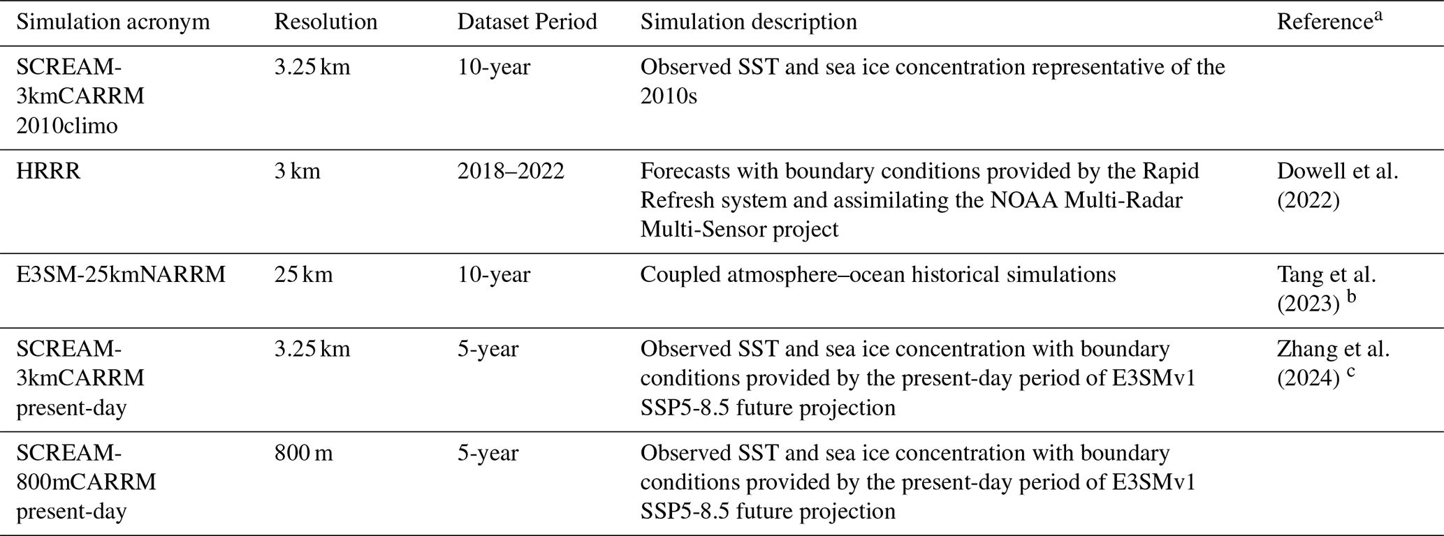
^a An empty or footnoted reference entry indicates that the simulation dataset was produced as part of this study. ^b Rerun to get the additional outputs used for energy modeling.
^c Rerun to use the same E3SMv1 boundary conditions as the SCREAM-800mCARRM present-day simulations.

The remainder of this paper is organized as follows. Section 2 describes the 3.25 km and 800 m SCREAM-CARRM configurations and other model outputs used to model wind and solar generation. Section 3 presents the simulation results and comparisons with observations. Section 4 discusses the implications and broader applicability of our findings.

2 Methods

This section describes the development and experimental design of the SCREAM-CARRMs used in this study, along with the other simulation datasets. Modeled CFs are computed by coupling meteorological outputs from SCREAM-CARRMs, E3SM-25kmNARRM, and HRRR with PySAM, and evaluated against monthly plant-level CFs from EIA as well as across the spatial distribution of California grid points.

2.1 Modeling strategy

2.1.1 Introduction to SCREAM

The 3.25 km and 800 m SCREAM-CARRMs are built upon SCREAM version 0 (SCREAMv0; Caldwell et al., 2021), developed under the E3SM project (Leung et al., 2020). SCREAM operates at a global horizontal resolution of 3.25 km, reaching convection-permitting scales without parameterizing deep convection. It uses 128 vertical layers on a hybrid coordinate, with vertical grid spacing increasing from 30 m near the surface to approximately 200 m at the boundary layer top, and a model top at roughly 40 km. The nonhydrostatic dynamical core is based on the HOMME (High-Order Methods Modeling Environment) framework (Taylor et al., 2020).

SCREAM’s physics suite includes Simplified Higher-Order Closure (SHOC; Bogenschutz and Krueger, 2013) for unified cloud macrophysics, turbulence, and shallow convection; Predicted Particle Properties (P3) microphysics (Morrison and Milbrandt, 2015); the Radiative Transfer for Energetics and Rapid Radiative Transfer Method for General circulation model applications – Parallel (RTE + RRTMGP) radiative transfer package (Pincus et al., 2019); and the Simple Prescribed Aerosol (SPA) module for aerosol properties (Mahfouz et al., 2025). Surface conditions are based on the E3SM land model (Golaz et al., 2019) and the Los Alamos prescribed CICE4 and data ocean models (Hunke et al., 2008). Land surface fluxes are based on Monin-Obukhov similarity theory, while surface fluxes over ocean are computed using a bulk formulation.

SCREAM Version 1 (SCREAMv1), implemented in C$++$/Kokkos, has been publicly released and documented (Donahue et al., 2024). RRM capability was not yet available in SCREAMv1 at the time of our simulations, so this study used SCREAMv0. Although GPU resources were unavailable during this study, separate work using similar SCREAM-RRM configurations (Zhang et al., 2026) has demonstrated significant GPU-enabled performance gains.

2.1.2 CARRM configuration

The 3.25 km and 800 m CARRMs generally follow the configurations in Zhang et al. (2024) and Bogenschutz et al. (2024). The 3kmCARRM mesh covers mainland California, adjacent offshore areas, and part of western Nevada. Outside this domain, a 1° global resolution is used, transitioning into the refined region via eighth-order refinement (Fig. 1a). The 800mCARRM mesh covers the same spatial extent but undergoes refinement to 800 m (Fig. 1b). Maximum Dinv-based element distortions are 3.02 for 3.25 km and 3.05 for 800 m meshes, indicating high-quality grids (Dinv is acceptable if below 4; it quantifies element shape distortion as the ratio of the maximum to minimum singular values obtained from a singular value decomposition (SVD) of the element mapping. See https://acme-climate.atlassian.net/wiki/spaces/DOC/pages/872579110/Running+E3SM+on+New+Atmosphere+Grids, last access: 25 June 2025). The land model operates on the same grid as the atmosphere, while the data ocean component uses the Model for Prediction Across Scales (MPAS) 18-to-6 km mesh (oRRS18to6v3).

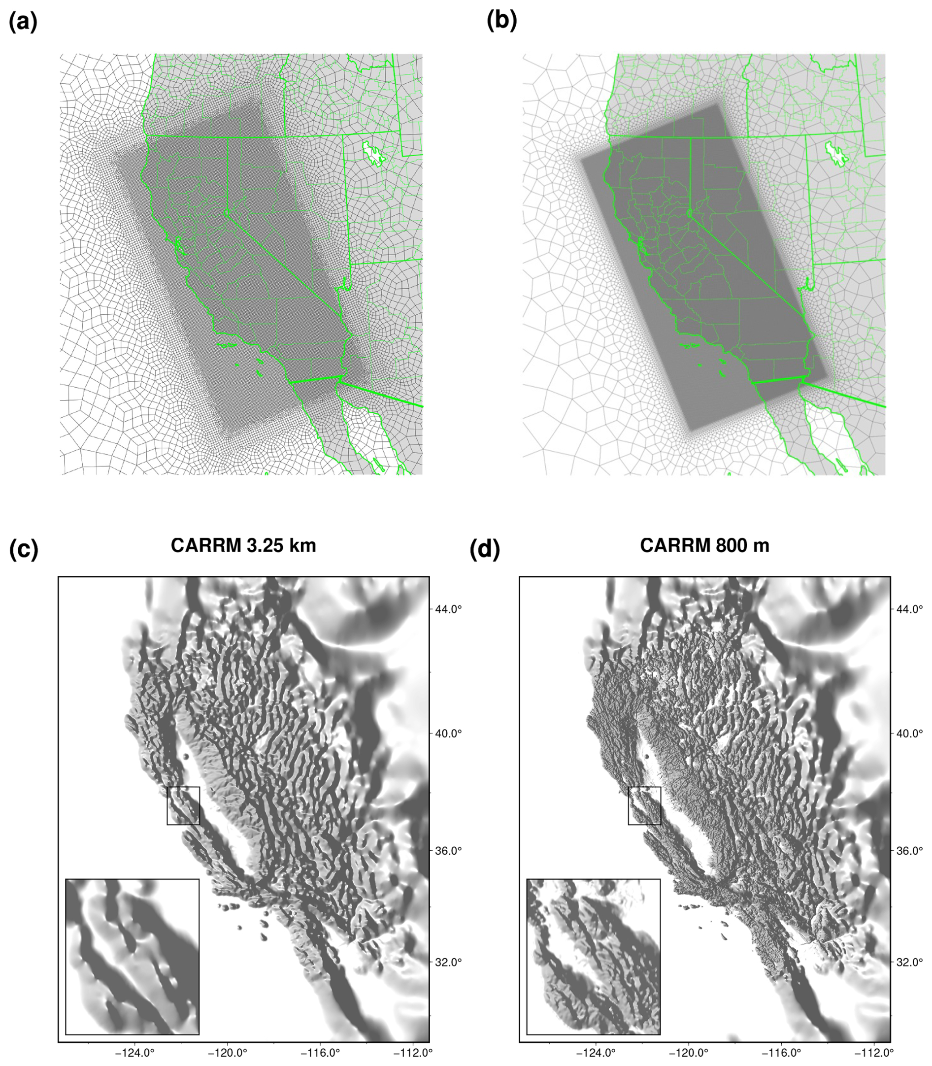
Figure 1 The grid of the (a) 3.25 km and (b) 800 m California regionally refined models. The topography of the (c) 3.25 km and (d) 800 m California regionally refined models, with the small rectangular box over part of the San Francisco Bay Area zoomed in.

The RRM workflow includes grid generation using SQuadGen v1.2.2 (Ullrich and Roesler, 2024), mapping/domain files, topography generation, land surface and land use data, and dry deposition files. Except for regenerating topography for 800mCARRM using higher-resolution digital elevation model (DEM) data, the workflow follows Zhang et al. (2024) and Bogenschutz et al. (2024). Specifically, the 800mCARRM uses the USGS GMTED2010 15 arcsec (500 m) DEM instead of the default GTOPO30 30 arcsec (1 km) DEM (Lauritzen et al., 2015). The 500 m GMTED2010 data were interpolated onto a global 800 m cubed-sphere grid to generate the 800mCARRM topography. The 3kmCARRM topography underwent 12 smoothing iterations, while the 800mCARRM used six, following the E3SM Version 3 workflow (https://acme-climate.atlassian.net/wiki/spaces/DOC/pages/2712338924/V3+Topography+GLL+PG2+grids, last access: 25 June 2025). Final topographies are shown in Fig. 1c and d.

Atmosphere initial conditions were generated with the HICCUP package (https://github.com/E3SM-Project/HICCUP, last access: 25 June 2025), which automates downloading and interpolating ERA5 pressure-level data. Vertical interpolation is performed by netCDF Operator (NCO) (Zender, 2008), while horizontal interpolation invokes various tools and algorithms through NCO. We employed NCO for linear-in-log(pressure) vertical interpolation and TempestRemap (Ullrich and Taylor, 2015; Ullrich et al., 2016) for high-order horizontal interpolation onto the RRM dynamical core grid. HICCUP also applies surface adjustments following Trenberth et al. (1993) to mitigate spurious gravity wave shocks associated with initial imbalances. Land initial conditions were taken from a well spun-up (1850–2015) 1° E3SMv1 historical simulation at 00:00 UTC on 1 January 2015 (Golaz et al., 2019). Notably, this historical simulation serves as the precursor to the future simulation used to generate nudging data, ensuring internal consistency.

2.1.3 Source of boundary conditions: 1° E3SMv1 simulations

SCREAM lacks a scale-aware deep convection scheme. In SCREAM-RRM global simulations, nudging is applied outside the high-resolution domain to constrain the large-scale circulation, thereby helping to maintain realistic large-scale thermodynamic and dynamical conditions in the absence of a convective parameterization. Prescribed SST and sea ice concentration boundary conditions are also necessary due to SCREAM’s atmosphere-land-only coupling. To ensure consistency across these boundary conditions, nudging variables and SST/sea ice concentration fields were obtained from a coarse-resolution E3SM simulation.

We conducted simulations with two different configurations to provide boundary conditions for the RRM simulations. The first is a rerun of a 1° fully coupled E3SMv1 simulation (Golaz et al., 2019), following the setup of Zhang et al. (2024), to produce 3-hourly fields of $U,V,T$, and Q (winds, temperature, and humidity) as well as monthly SST and sea ice concentration. Although this simulation follows the SSP5-8.5 pathway (Zheng et al., 2022), our analysis focuses only on the nominal 2015–2020 water-year period (October–September accounting year used in hydrology), where radiative forcings and global climate statistics closely resemble those of the present day (e.g., Kriegler et al., 2017). We refer to this configuration as the “present-day” simulation. In parallel, we conducted a 10-year E3SMv1 simulation using forcings representative of the 2010s, in which SST and sea ice are prescribed from the monthly climatology averaged over 2005–2014. This type of experiment simulates the atmosphere–land components interactively with prescribed ocean conditions. It is widely used for evaluating model performance against observational data. We refer to this configuration as the “2010climo” simulation.

Nudging data are interpolated onto the RRM physics grid using NCO’s linear-in-log-pressure vertical interpolation and TempestRemap’s high-order horizontal interpolation. Nudging of $U,V,T$, and Q with a 2 d relaxation timescale is applied following Zhang et al. (2024). Regional nudging in E3SM employs a tanh-based smooth windowing function that is zero within the refined region and transitions toward one in the surrounding coarse-resolution domain (e.g., Tang et al., 2019), allowing free-running conditions over California and applying nudging in the coarser-resolution domain. Vertically, the default tanh-based smooth window is applied, which reduces the effective nudging strength near the surface and at the top and full strength in between.

SSTs and sea ice concentrations were processed using the e3sm_to_cmip tool (https://github.com/E3SM-Project/e3sm_to_cmip, last access: 25 June 2025), converting MPAS outputs to 1° lat-lon time series. Missing land values were filled via Poisson equation relaxation before formatting into Data Ocean stream files (https://esmci.github.io/cime/versions/ufs_release_v1.1/html/data_models/data-ocean.html, last access: 25 June 2025).

2.1.4 Timestep and computational cost

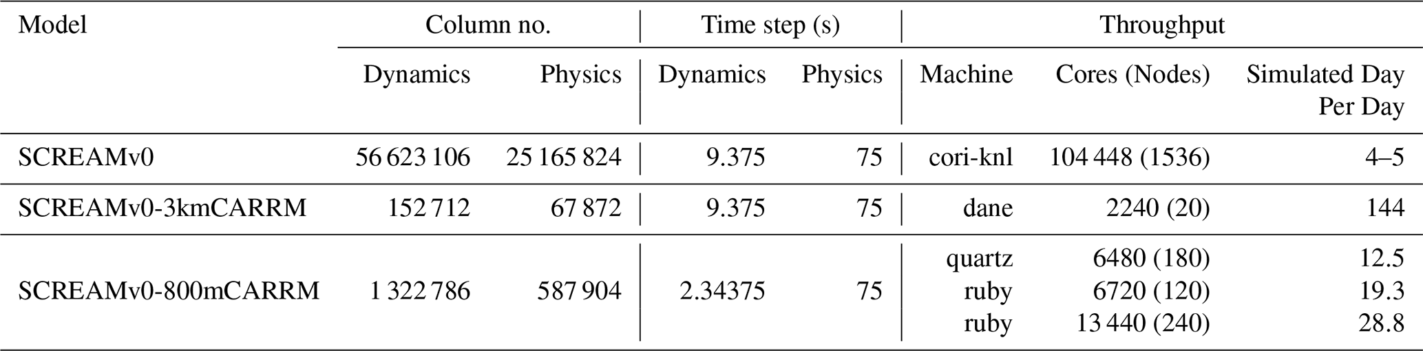
The 3kmCARRM grid (67 872 physics columns; Zhang et al., 2024) comprises only 0.27 % of the global 3.25 km SCREAM physics columns (25, 165, 824 physics columns; Caldwell et al., 2021), while the 800mCARRM grid (587, 904 columns; Bogenschutz et al., 2024) represents 2.3 %, significantly reducing storage and computational costs compared to a global km-scale model.

All SCREAM-CARRM simulations were conducted on the Livermore Computing (LC) clusters Ruby, Dane, and Quartz. Ruby nodes feature 56 Intel(R) Xeon(R) Platinum 8276 CPUs @ 2.20 GHz; Dane nodes feature 112 Intel(R) Xeon(R) Platinum 8480+ CPUs @ 2.0 GHz; and Quartz nodes are equipped with 36 Intel(R) Xeon(R) E5-2695 v4 CPUs @ 2.10 GHz. For SCREAM-3kmCARRM 2010climo and present-day simulations, 20 Dane nodes were used. The SCREAM-800mCARRM present-day simulation incurred substantially higher computational costs and was executed in two phases due to machine and project transitions. The first phase used 180 Quartz nodes (1 October 2015–4 January 2017), followed by a second phase using 120 Ruby nodes (4 January–1 October 2017) and 240 Ruby nodes (1 October 2017–1 October 2020). All simulations used MPI-only processes, with no OpenMP threads.

The 3kmCARRM simulations advanced at a pace of approximately 144 simulated days per wall-clock day (including I/O overhead), running one simulation month per job submission. The 800mCARRM simulation was conducted in 10 d chunks, achieving throughputs of about 12.5 simulated days per day on 180 Quartz nodes, and about 19.3 simulated days per day on 60 Dane nodes. During the 5-year SCREAM-3kmCARRM present-day simulation, four “EOS (equation of state) bad state” failures occurred; five such failures occurred during the 10-year 2010climo simulation. These errors arise when the model’s thermodynamic variables violate the equation of state (EOS), which governs the physical relationship among pressure, temperature, and density. No EOS failures were seen in the 800mCARRM simulation. Each EOS error was resolved by temporarily halving the dynamical core timestep for one job cycle before reverting to the default timestep. All simulation outputs have been archived.

Table 2 compares the column counts, timesteps, and throughputs between the 3.25 km and 800 m SCREAMv0-CARRMs and the global SCREAMv0 3.25 km simulation in Caldwell et al. (2021).

Table 2 Column numbers, timesteps, and throughputs of SCREAMv0 global 3.25 km simulation, 3kmCARRM, and 800mCARRM.

2.2 Evaluation strategy

This section introduces the evaluation strategy for modeled CFs. The plant-level EIA monthly data were first processed by reading raw tables, applying quality control, filtering valid plants, and aggregating them to model grids. Wind and solar CFs were then computed by coupling model outputs with EIA plant locations within our PySAM preprocessing pipeline. Additional simulation datasets and PLUSWIND-provided CFs beyond the SCREAM and E3SM simulations are also introduced. Finally, to better diagnose CF discrepancies and provide a broader perspective, we calculate CFs over all California grid points and analyze the spatial distribution of key input variables as well as the large-scale circulation that modulate them.

2.2.1 EIA monthly CF data

EIA provides plant-level electricity generation data through monthly generation records from EIA-923 (https://www.eia.gov/electricity/data/eia923/, last access: 25 June 2025) and generator-specific metadata for plants with nameplate capacities over 1 megawatt from EIA-860 (https://www.eia.gov/electricity/data/eia860/, last access: 25 June 2025).

The EIA-processor package extracts and preprocesses EIA data to produce monthly wind and solar CFs for 2013–2024 (Lee et al., 2026). It reads generation values from the “Netgen” column in EIA-923 and retrieves plant attributes (“Plant Code”, “Plant Name”, “State”, “County”, “Latitude”, “Longitude”, “Nameplate Capacity”, “Technology”, and “Axis Tracking”) from EIA-860. Initial quality control and duplicate removal were incorporated during EIA preprocessing.

The EIA data first underwent the following plant-level quality control steps:

1. Only plants with a nameplate capacity of at least 2.5 MW were included.

2. Only plants located in the state of California were included.

3. For solar generation, only plants classified as “Solar Photovoltaic” were retained (accounting for 97.3 % of all solar facilities), while those categorized as “Solar Thermal without Energy Storage” were excluded. In this study, the term solar refers specifically to PV (photovoltaic) power.

4. For solar PV plants, only those with a reported array configuration in the EIA dataset were retained, as indicated by at least one of the fields “Single-Axis Tracking?”, “Dual-Axis Tracking?”, or “Fixed Tilt?”.

5. Plants were excluded if CF was below 5 % for more than nine months or if more than 12 months of data were missing.

These quality control steps resulted in 72 valid wind plants and 322 PV plants.

To align with the model resolution, the geographical locations (latitude and longitude) of individual plants reported in the EIA data were aggregated to the target model grid. For the 3kmCARRM grid, this process aggregated all valid wind plants and PV plants into 32 and 222 model grid points, respectively. In the subsequent analysis, wind plants are clustered based on geographical location, while PV plants are clustered by axis-tracking type.

We adopted a gridcell-based evaluation framework instead of plant-level evaluation for the following reasons: (1) It avoids artificially reducing the spread of the modeled climatological seasonal cycle. In plant-level evaluations, multiple plants located within the same model grid cell would be represented identically. This would substantially reduce the apparent monthly climatological spread and make modeled variability appear artificially smaller than that from observations. (2) Aggregating to the model grid ensures consistency between local evaluations and assessments of spatial patterns across California, as both are conducted on the same grid. In the seasonal-cycle analysis, we applied a weighted average based on total nameplate capacity within each grid cell, so that the EIA mean line remains consistent across comparisons at different model resolutions.

For wind plants, because all quality control is applied at the plant level, and the clustering logic does not depend on plant-specific attributes, aggregating to different model grids does not affect the total nameplate capacity of each cluster. For PV plants, we group samples by both model grid point and axis-tracking type. For example, if a grid point G contains three single-axis plants and one fixed-axis plant, two groups are formed: G₁ (single-axis) and G₀ (fixed). The seasonal cycles and evaluation metrics are then computed by clustering according to axis-tracking type. This approach preserves the plant-level tracking type information reported in the EIA dataset, and the total nameplate capacity within each cluster does not vary with model resolution. As will be shown in the results section, the axis-tracking type has a substantial influence on PV power generation.

Finally, we applied an “independent-plant ratio > 15 %” threshold to all valid EIA plants. The independent-plant ratio is defined as the fraction of plants in a given year whose monthly CF time series are not perfectly correlated with those of other plants (identified using a Pearson correlation distance threshold of 10⁻⁶). This was motivated by the fact that the EIA data contains many plants that only report annual values without providing monthly records, for which seasonal variability is imputed from other plants. The background of this issue and the investigation that led to this finding are described in Appendix A. Applying this threshold removes years heavily affected by plants with imputed data, correcting the artificial reversal of the seasonal phase – compared to all models – at the Shasta wind plant and adjusting seasonal peaks in northern California, while having minimal impact elsewhere.

2.2.2 PLUSWIND-derived CFs

PLUSWIND (Millstein et al., 2023) provides hourly, plant-level generation estimates across the U.S. from 2018 to 2021, using meteorological inputs from three models: ERA5, MERRA2, and HRRR. They use hub-height wind speeds from HRRR, model-level wind speeds from ERA5, and near-surface wind speeds from MERRA2 to estimate wind power generation.

To improve plant geolocation, PLUSWIND computed wind plant centroids from the U.S. Wind Turbine Database (USWTDB; Rand et al., 2020) rather than relying on the self-reported EIA-860 coordinates. Each plant was matched to a representative wind turbine power curve based on key assumptions: (1) a cut-in speed of 3 m s⁻¹, (2) a cut-out speed of 25 m s⁻¹, and (3) a rated speed between 9–13 m s⁻¹, derived from the plant’s average specific power, which was calculated from turbine diameter and capacity. Hub-height wind speeds were estimated differently across models: for ERA5, by vertical interpolation from model levels; for MERRA2, by applying a log wind profile using 2, 10, and 50 m wind speeds; and for HRRR, directly without additional correction. For repowered plants, data from the repowering year were excluded, and turbine characteristics were updated to the most recent configuration for all years. Air density correction for all models (ERA5, MERRA2, HRRR) was based on MERRA2 air density, interpolated to hourly resolution at hub height. Wake losses were estimated using a simple method: a constant 7 % loss was applied when wind speeds fall below rated speed minus 0.5 m s⁻¹, tapering linearly to zero at rated speed plus 2 m s⁻¹.

2.2.3 Coupling with PySAM to estimate wind and solar CFs

All SCREAM-CARRM simulations output hourly meteorological variables, including surface pressure, 2 m temperature, 2 m relative humidity (used with temperature to derive the dew point), downward shortwave radiation (total and diffuse components), hub-height winds at 90, 10 m winds, and snow water equivalent. Together with static surface geopotential height, these variables serve as inputs for CF calculations through PySAM. HRRR provides the same set of hourly variables, except that hub-height wind is reported at 80 m instead of 90 m.

Developed by the National Laboratory of the Rockies (NLR), the System Advisor Model (SAM) (https://sam.nlr.gov/, last access: 20 March 2026) provides a comprehensive set of algorithms and assumptions for calculating electricity generation and approximating CFs (i.e., actual generation divided by nameplate capacity). PySAM is the Python wrapper of SAM (https://github.com/NatLabRockies/pysam, last access: 20 March 2026).

In this study, we used our preprocessing pipeline developed for PySAM (, ) to calculate hourly generation outputs: wind power was estimated using PySAM.Windpower.default(“WindPowerNone”) and solar PV power using PySAM.Pvsamv1.default(“FlatPlatePVNone”).

The default parameter set was used for PySAM.Windpower.default(“WindPowerNone”), including the use of a generic turbine power curve without plant- or manufacturer-specific corrections, which neglects variations in turbine physical characteristics such as rotor diameter and rated capacity, and the use of fixed 90 m hub-height wind inputs without turbine-specific height correction. The default wake calculation includes the simple wake model (https://samrepo.nrelcloud.org/help/wind_power.html, last access: 20 February 2026), together with an external wake loss of 1.1 %. The simple wake model computes distances between downwind and crosswind turbines based on their relative positions within a wind farm and accounts for the effects of power coefficient, thrust coefficient, and turbulence intensity on wind speed. The default parameter set specifies relative x and y coordinates for 32 turbines within a generic wind farm. Because the primary focus of this study is model evaluation and the complexity of meteorological datasets, we chose to follow the default settings in PySAM to maintain focus.

The PySAM.Pvsamv1.default(“FlatPlatePVNone”) configuration is a detailed PV model that includes separate representations of the module, inverter, and cell temperature. The default use of nominal operating cell temperature (NOCT) model (Gilman et al., 2018) relies on effective irradiance transmitted to the cell, air temperature, and near-surface wind speed. In addition to the default fixed-axis tracking configuration, single- and dual-axis tracking configurations are enabled by setting SystemDesign.subarray1_track_mode. The default option None is used for subarray shading, meaning no self-shading or backtracking is applied to avoid row shading.

Required inputs to PySAM include:

1. Locations (latitude, longitude) of power plants within California reported by EIA;

2. Hourly simulation outputs reformatted into a full-year (365 d calendar) 8760 h time series, with each variable stored in a separate file. Model grid points corresponding to plant locations were identified using the BallTree class from the sklearn.neighbors module (https://scikit-learn.org/1.6/, last access: 25 June 2025);

3. For solar PV, axis tracking types (fixed, single-axis, dual-axis) reported by EIA were assigned by setting SystemDesign.subarray1_track_mode to 0, 1, or 2, respectively, across all sub-arrays.

Note that the EIA data are reported after curtailment, whereas our generation modeling does not include this effect. As a reference, Lee et al. (2026) applied a curtailment correction of 2 % for wind and 3 % for solar CFs over California.

Executing our PySAM preprocessing pipeline generated hourly CFs for each power plant across all SCREAM-CARRM simulations, HRRR, and E3SM-25kmNARRM.

2.2.4 HRRR

Inspired by the PLUSWIND dataset, we evaluate the HRRR (Dowell et al., 2022) as an additional source of meteorological data to drive PySAM, given that its horizontal and boundary-layer vertical resolutions are comparable to SCREAM-CARRMs. HRRR assimilated conventional observations and radar reflectivity at each forecast cycle and remains the highest-resolution historical forecast dataset over North America.

We used HRRR +1 h forecasts from 2018 to 2022, substituting +2 or +3 h analyses when +1 h data are unavailable. Despite model biases and PySAM assumption errors, HRRR is expected to perform well due to its frequent data assimilation. In fact, HRRR is widely used in the wind energy industry (Shaw et al., 2019). Thus, HRRR provides another reference for assessing SCREAM-RRM performance in electricity generation. Among the three SCREAM-CARRM simulations, the 3kmCARRM 2010climo experiment design aligns most closely with HRRR, offering comparable resolution and similar climatology. Key differences arise from model structure, data assimilation, and internal variability (i.e., 2010climo is a 10-year simulation using 2010s SST, whereas HRRR is a 5-year simulation driven by evolving SST from 2018 to 2022).

We also compare HRRR-modeled wind CFs from PLUSWIND with our PySAM-derived results to isolate sensitivities to wind power modeling assumptions. These sensitivities are further compared with sensitivities to model structure (HRRR vs. SCREAM-3kmCARRM 2010climo), and to resolution (HRRR vs. ERA5/MERRA2 in PLUSWIND; SCREAM-3kmCARRM vs. SCREAM-800mCARRM vs. E3SM-25kmNARRM).

2.2.5 Statewide CFs, meteorological drivers, and large-scale circulation

To better understand the differences in CFs derived from different simulations, we extend our analysis beyond EIA plant locations and estimate CFs at all grid points across California using PySAM. This provides a comprehensive spatial view of wind and solar resource availability within the state and enables direct comparison with local topography and meteorological drivers. We present the spatial distributions of variables directly used in PySAM calculations over California including: 2 m temperature, 90 m hub-height winds, and total downwelling solar flux at the surface, alongside global-scale atmospheric circulation patterns. ERA5 is used as a reference to evaluate model biases in both the regional meteorological fields and the large-scale circulation. However, some ERA5 variables (such as hub-height wind speeds) are less reliable for evaluating km-scale models as they are strongly affected by topographic features (e.g., Millstein et al., 2022, 2023).

3 Results

This section begins by discussing some of the data limitations and clarifies our interpretation of the comparison results given these obstacles. We also outline the structure and rationale of our evaluation groups. We then present the results sequentially, organized under two main categories: wind and solar.

3.1 Uncertainty in EIA monthly data and interpretation of discrepancies

A fundamental issue with the monthly EIA data is that the procedures used for collecting and processing are not publicly known, particularly how missing data, outages, curtailments, and obvious anomalies are handled during temporal averaging (see similar discussion in Ryberg et al., 2019). Another limitation is the issue of non-independent samples associated with plants with imputed data, as discussed in the “Methods: EIA monthly CF data” section and Appendix A. Therefore, we cannot assert that generation estimates from model outputs are inherently erroneous, nor can we determine the true degree of error. The difference between model-simulated and EIA-reported CFs should be viewed not as a conventional model bias, but rather as a discrepancy. Nevertheless, for convenience, we retain the term bias in parts of the discussion or figures as a well-defined statistical quantity relative to EIA, without implying that EIA provides a ground truth or that model–data differences arise solely from model deficiencies.

In principle, the most accurate model evaluation data would ideally come from on-site meteorological towers or remote sensing systems, such as lidar or meteorological masts deployed by wind plant developers, which could provide high-quality wind speed observations. However, such data are expensive, technically challenging to obtain, and not publicly available (Jourdier et al., 2020; Pronk et al., 2022). Widely available meteorological station data are typically limited to near-surface (10 m) observations, which are insufficient for direct wind power evaluation. Previous studies have shown that interannual variability in wind power generation is only weakly correlated with observed near-surface wind speed (Millstein et al., 2022), motivating PLUSWIND to evaluate HRRR using EIA generation data rather than surface wind observations. Extrapolating 10 m winds to hub height requires power-law assumptions, whose exponents depend on atmospheric stability and surface roughness and are known to perform poorly under stable conditions (Frank et al., 2020). This is particularly relevant in California, where wind power generation tends to be stronger at night (Millstein et al., 2023) when atmospheric stability is higher.

An alternative and more direct observational benchmark would be high-frequency (e.g., hourly) plant-level generation data, which retain diurnal and weather-scale variability and could better capture generation losses associated with disruptive meteorological or hydrological events (Davidson and Millstein, 2022). Unfortunately, such data are not publicly available for California at the plant level. Monthly CFs, while inevitably smoothing sub-hourly and synoptic-scale variability, therefore remain the only feasible observational constraint for statewide evaluation.

Given these limitations, the use of monthly EIA data in this study reflects a trade-off between observational fidelity and data availability. We therefore caution against attributing discrepancies between modeled generation and EIA monthly CFs solely to deficiencies in either the atmospheric simulations or the power generation modeling. Instead, these discrepancies should be interpreted in light of the combined uncertainties inherent in both the observational data and the meteorological–generation modeling framework. This is why we also include comparisons with PLUSWIND and HRRR to help assess the relative importance of different uncertainty sources.

3.2 Evaluation design and structure

The Results section is organized to address the three guiding questions introduced in the Introduction through a set of controlled comparisons. All CFs are calculated using a consistent PySAM configuration unless otherwise noted. Because discrepancies relative to EIA reflect combined uncertainties from meteorological datasets, power-generation modeling, and EIA data quality, additional benchmarks are introduced to help contextualize the relative importance of these uncertainty sources.

For both wind and solar energy, the analysis follows a common structure:

1. Generation model dependence (Q1). For wind, we compare CFs derived from HRRR using PLUSWIND and PySAM to assess whether generation model choices materially affect CF estimates. For solar PV, we quantify the sensitivity of modeled CFs to axis-tracking assumptions within PySAM. These tests serve as a validation of PySAM before inter-comparing meteorological datasets.

2. Meteorological dataset dependence at comparable resolution (Q2). We compare SCREAM-3kmCARRM 2010climo against HRRR, both of which provide km-scale meteorological fields to PySAM. This comparison quantifies the magnitude of CF differences attributable to the meteorological model when horizontal resolution is not the primary differentiator.

3. Horizontal resolution sensitivity (Q3). We compare present-day SCREAM-CARRM simulations at 3.25 km with the E3SM-25kmNARRM simulation to assess whether km-scale configurations substantially reduce the pronounced wind CF phase errors identified at 25 km resolution over California. Sensitivity to further refinement of resolution is then examined by comparing the 3.25 km and 800 m CARRM simulations.

Within each comparison group, results are presented separately for wind and solar. For each energy type, we first show multi-year monthly CF climatology aggregated by plant clusters, followed by diagnostics that help interpret CF differences, including diurnal cycles of simulated CFs, statewide spatial patterns of CFs and key meteorological driver variables used by PySAM. Each energy-type section concludes with a summary plot to synthesize the main findings across meteorological datasets.

3.3 Wind

3.3.1 Does the use of different energy models affect wind CFs?

Figure 2 shows our selected groupings for wind plants. We clustered geographically because wind simulations depend strongly on topographic features and surface type. Wind resources at each location are driven by multiscale atmospheric dynamics. Large-scale circulation, synoptic patterns, and geopotential gradients drive synoptic flows that are influenced by coastal proximity. At smaller scales, topography and land-surface heterogeneity govern mesoscale to microscale effects, such as mountain-valley circulations and buoyancy-driven flows. Additionally, winds are influenced by heterogeneous surface roughness that includes different vegetation types (e.g., grassland, forest canopy), urban areas, and water surfaces.

Figure 2 Clusters of wind plants across California, grouped by geographic proximity. Each cluster is marked with a green ellipse and annotated with the county name and number of plants. EIA plants are aggregated to the 3kmCARRM model grid; each filled dot represents the mean wind CF (%) from valid monthly EIA records between 2013 and 2024.

We define three plant groups in California: (1) “NorCal”, including 3 grid points (counted based on the 3kmCARRM model grid) in Solano County, 3 in Alameda County, and 2 in Contra Costa County, with a total installed capacity of 910.1 MW, (2) “Kern” grid points as a standalone category, given its large sample size (12 grid points) and a total installed capacity of 3322.5 MW, and (3) “SoCal”, including 4 grid points in Riverside County and 2 in San Diego County, with a total installed capacity of 696.8 MW. Each cluster is weighted by the nameplate capacity summed across all plants assigned to each model grid point, ensuring integral conservation.

The northernmost part of California contains only one power plant – Shasta. The Shasta plant is part of the Hatchet Ridge Wind Project, which consists of 44 turbines with a total nameplate capacity of 101.2 MW. In our analysis, we found that Shasta exhibited a distinct wind CF seasonal pattern: it peaks in summer, in phase with the rest of California in the EIA monthly records, but out of phase with all modeled patterns. The analysis of Shasta confirmed the data imputation issue in the EIA data (see “Methods: EIA monthly CF data” section and Appendix A for details). By excluding years with too few independent samples, the artificial seasonal cycle at Shasta was corrected (Fig. A3a). However, given the small sample size (N=1) relative to other regions, we exclude the Shasta site from further analysis. The only other single-sample case is in Santa Barbara, where data passed quality control only for 2024.

Figure 3 presents a comparison of modeled CFs for different generation modeling, including PLUSWIND and PySAM. All CF differences are expressed in percentage points (pp) in the following text. In PLUSWIND, ERA5 (yellow) produces the lowest CFs, followed by MERRA2 (orange), with both staying below EIA values throughout the year and across all geographic clusters (see more discussions in Dowell et al., 2022). HRRR (red) in PLUSWIND gives the highest CFs, typically exceeding EIA, especially in Kern and SoCal (by 10–25 pp). PLUSWIND computes three different generation outputs for each model: raw estimates (dotted), density-adjusted (dashed), and density + loss adjusted (solid). The impact of these assumptions is secondary to the choice of meteorological model, highlighting that the generation modeling assumptions in PLUSWIND are a minor source of uncertainty.

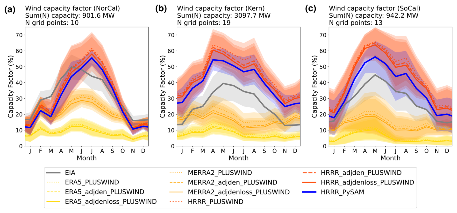
Figure 3 Seasonal variation in wind CFs (%) estimated using different generation modeling options, including PLUSWIND and PySAM. Each subplot corresponds to a cluster in Fig. 2. Different meteorological datasets in PLUSWIND are color-coded: ERA5 (yellow), MERRA2 (orange), and HRRR (red). For each dataset, different generation modeling assumptions by PLUSWIND are shown using line styles: default (dotted), air-density adjusted (dashed), and both air-density and loss adjusted (solid). PySAM-estimated generation from HRRR is shown in solid blue, and EIA data is shown in gray. The bold line shows the multi-year climatology, with shading indicating ±1 standard deviation.

PySAM-modeled HRRR estimates (solid blue) show similar seasonal patterns to those from PLUSWIND (solid red) but are overall lower by 2–8 pp, and generally closer to EIA. This suggests that the effect of modeling assumptions (turbine power curves, density estimation, wake losses) between PLUSWIND and PySAM is larger than the effect of internal corrections within PLUSWIND, but much smaller than the effect of varying meteorological model datasets.

Note that we first tested two plant coordinates when inputting HRRR data into PySAM: one based on EIA-reported plant locations (default), and the other based on PLUSWIND-provided coordinates derived from USWTDB centroids. The resulting CF differences were minimal (not shown). This is likely due to plant aggregation on the model grid. For HRRR and CARRMs, this grid is km-scale, which remains considerably coarser than the footprint of an individual plant. Therefore, spatial uncertainty from plant location has negligible impact on modeled generation.

PLUSWIND uses more realistic turbine power curves compared to the uniform default curve in PySAM’s default(“WindPowerNone”) configuration. While PySAM supports more detailed, plant-specific wind simulations (e.g., customized turbine parameters and variable hub heights), we used the default configuration to ensure consistency and simplicity across datasets. In addition, PLUSWIND applies MERRA2 air density correction and empirical losses of about 7 % to all model datasets. In contrast, PySAM uses near-surface temperature and humidity from each model to derive air density directly, and applies different loss assumptions. This might help explain why PLUSWIND estimates are different from PySAM.

In summary, generation modeling assumptions, especially air density and wake loss estimation, do influence CF outcomes. The differences between PLUSWIND and PySAM are more substantial than the variations introduced by internal assumptions within PLUSWIND itself. In general, PySAM’s estimates for California wind generation align more closely with EIA data. Nevertheless, the impact of generation assumptions is minor relative to the much larger discrepancy driven by meteorological inputs from different models.

3.3.2 How different are wind CFs between SCREAM-3kmCARRM and HRRR at comparable horizontal resolution?

Figure 4 presents the second evaluation group comparing wind power generation estimates from SCREAM-3kmCARRM 2010climo and HRRR, both processed using PySAM. HRRR, assimilating high-frequency observations, effectively functions as a km-scale reanalysis product, with internal variability closely aligned with historical conditions (2018–2022). The 10-year SCREAM-3kmCARRM simulation is forced by a repeating 2010s climatology for SST and sea ice concentration, resulting in weaker interannual variability.

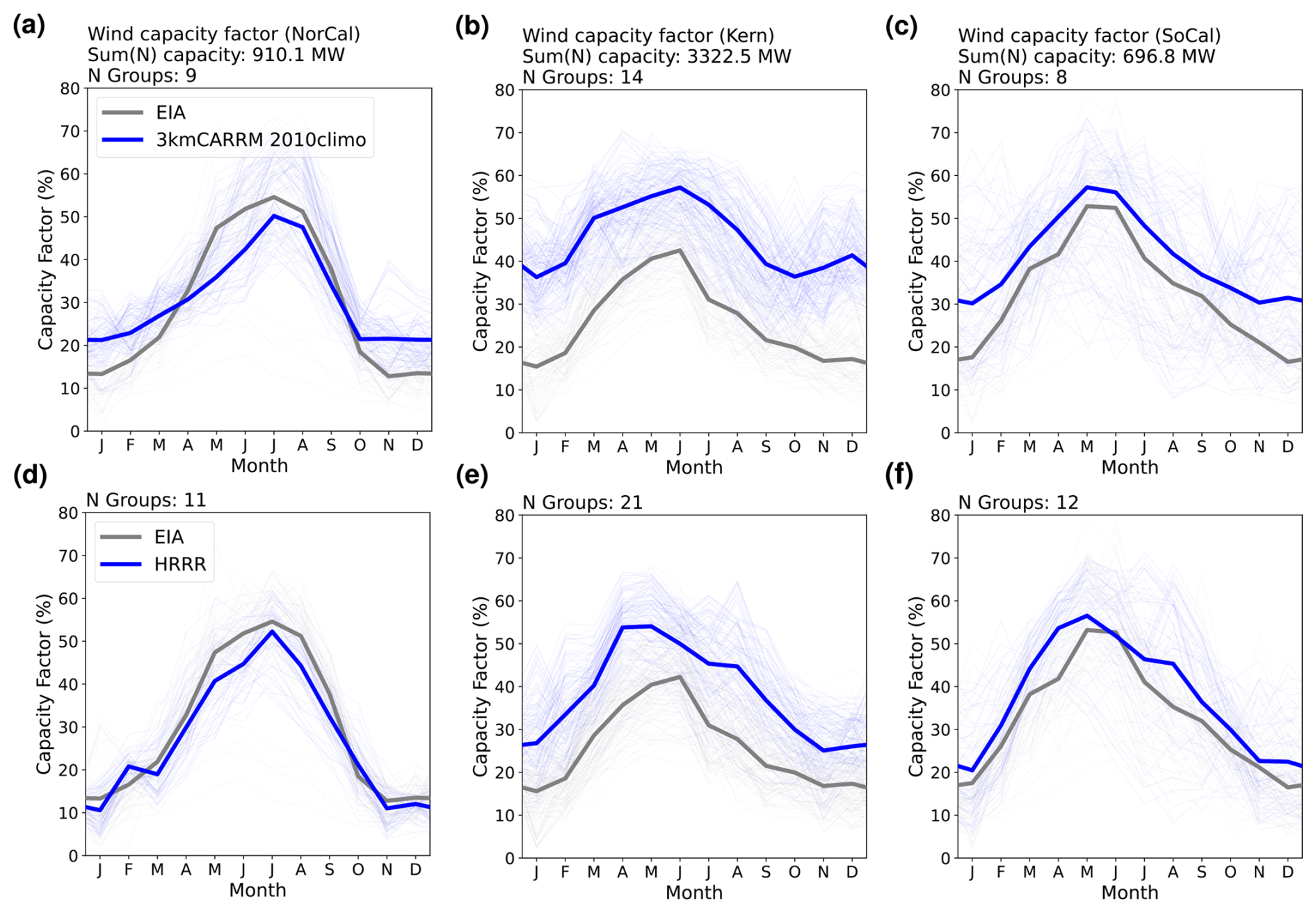
Figure 4 Seasonal variation in wind CFs (%) estimated using PySAM from SCREAM-3kmCARRM 2010climo (top) and HRRR (bottom). Each subplot corresponds to a cluster in Fig. 2. Simulations are shown in blue, and EIA records in gray. Light lines represent individual years; bold lines represent the multi-year climatology.

Overall, HRRR and SCREAM-3kmCARRM produce similar results, with differences substantially smaller than those between HRRR and MERRA2/ERA5 in PLUSWIND (Fig. 3). Considering the structural differences between HRRR and SCREAM (e.g., dynamics, physics parameterizations, and data assimilation/nudging) this suggests that horizontal resolution, rather than model structural details, exerts a first-order control on wind energy simulations. Note that the nominal resolution of 3.25 km refers to SCREAM’s dynamical core, while its physical grid has a resolution of ∼ 4.5 km, slightly coarser than HRRR. While this could lead to marginal degradation in results, wind simulations at km-scale are likely dominated by resolved processes, with limited sensitivity to turbulence scheme differences. This is consistent with findings from Altamont Pass, where two planetary boundary layer schemes in Weather Research and Forecasting model produced comparable performance in simulating wind conditions and CFs at similar resolution (Arthur et al., 2025b).

In terms of discrepancies between modeled CFs and EIA records across plant clusters, the largest occurs in Kern County. Note that we did not add a curtailment correction to the PySAM outputs; given the 2 % curtailment applied by Lee et al. (2026) to California wind energy, this is unlikely to explain the majority of the discrepancies. On the multi-year average, HRRR aligns more closely with EIA in this region, with an annual discrepancy of 13 pp. In contrast, SCREAM-3kmCARRM’s discrepancy in Kern increases from 15 pp in summer to 25 pp in winter. A similar seasonal pattern is observed in SoCal, where 3kmCARRM’s discrepancy grows from 10 to 15 pp between summer and winter. In the same region, HRRR’s overestimation declines from 10 pp in summer and fall to only 3 pp in winter. For NorCal, both models captured the summer peak well. During winter, 3kmCARRM tends to overestimate by 10 pp, while HRRR underestimates by 4 pp. SoCal shows the smallest discrepancy (< 5 pp) among all clusters, especially during spring and fall.

In summary, the two fundamentally different meteorological models (SCREAM-3kmCARRM and HRRR) produce overall similar wind generation estimates when using comparable horizontal resolution, with HRRR results closer to EIA values. Given HRRR’s nature as a reanalysis-like product, its lower discrepancy might be expected. Additionally, we find that 3kmCARRM consistently overestimates winter wind generation relative to summer, whereas HRRR does not exhibit this pattern. This may indicate a systematic wintertime wind bias in SCREAM-CARRMs.

3.3.3 How much does horizontal resolution affect wind energy?

Figure 5 presents California wind energy estimates from E3SM-25kmNARRM, as well as the 3.25 km and 800 m SCREAM-CARRM present-day simulations, all processed using PySAM. The only difference between the two SCREAM-CARRM simulations is horizontal resolution. SCREAM-CARRMs and E3SM-25kmNARRM differ in several aspects, including resolution, physical parameterizations, and internal variability.

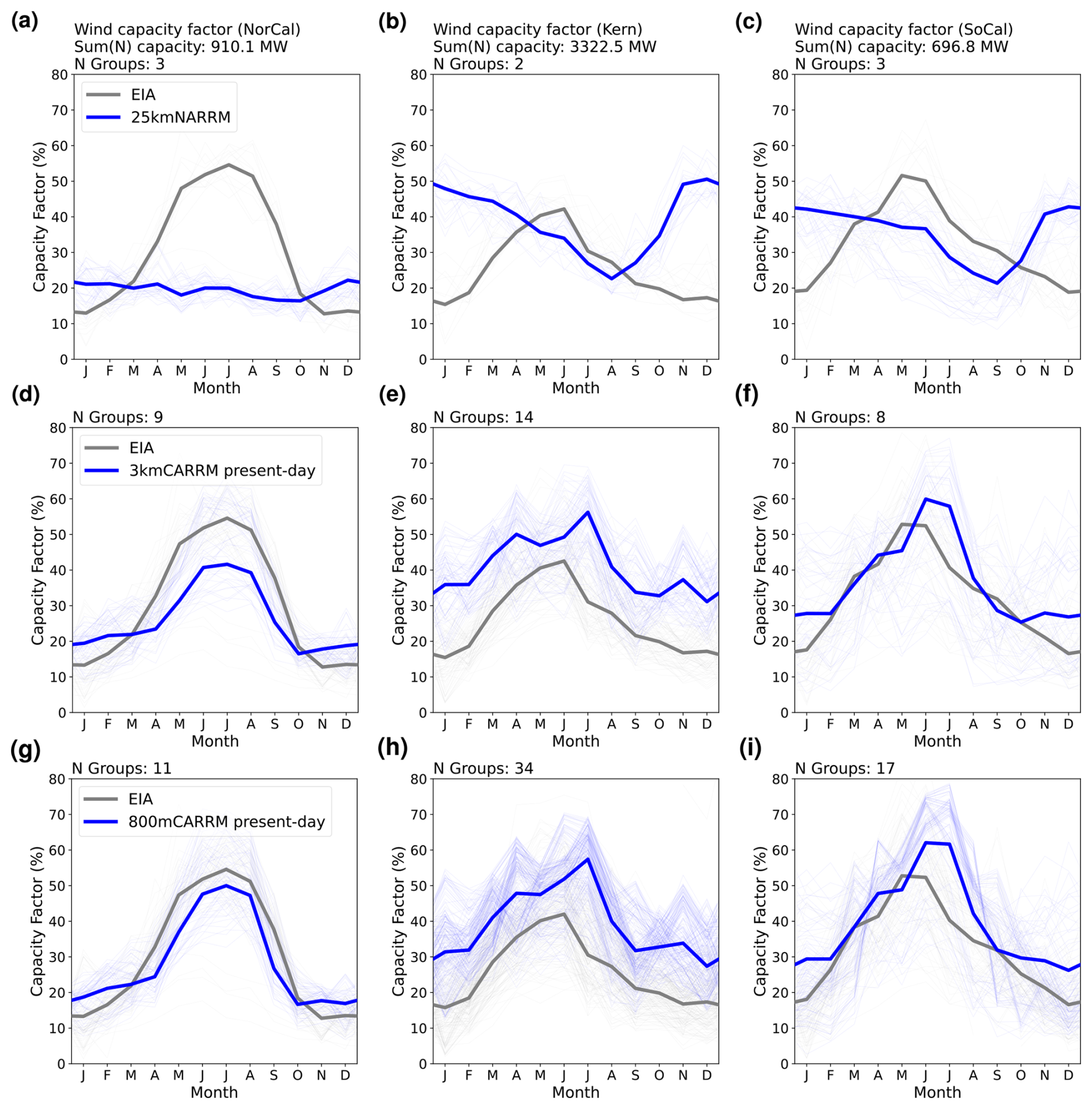
Figure 5 As in Fig. 4, but comparing (a–c) E3SM-25kmNARRM simulations with (d–f) 3.25 km and (g–i) 800 m SCREAM-CARRM present-day simulations.

Strikingly, the E3SM-25kmNARRM simulation shows either a near-reversal or a strong damping of seasonal variability in wind generation across California. This pattern was first identified by Lee et al. (2026). In contrast, the SCREAM-3kmCARRM simulation captures the EIA seasonal phase much more accurately, with clear improvements particularly in seasonal timing. Since all EIA processing, PySAM configuration, and data filtering were held constant in our analysis, the differences seen here can be attributed solely to the meteorological models. Resolution plays a far more dominant role than large-scale circulation, as shown in the next section, where similar large-scale patterns still lead to substantial differences due to resolution.

For the 3.25 km vs. 800 m SCREAM-CARRM simulations, the modeled wind CFs differ only slightly. In Kern and SoCal, wintertime generation from SCREAM-800mCARRM is closer to EIA, with discrepancies reduced by 5 pp compared to the 15–20 pp overestimation from SCREAM-3kmCARRM. However, during summer (particularly in July) overestimation increases with resolution across NorCal, Kern, and SoCal. This suggests that a 4× increase in resolution yields only modest sensitivity in SCREAM wind generation estimates, with no consistent improvement in the match to EIA, as quantified by the summary of absolute differences shown in Fig. 9 (Sect. 3.3.6). Note that both simulations are based on present-day forcing, not observed SST and sea ice concentration, so their discrepancies relative to EIA are larger than those in Fig. 4. Therefore, the discrepancy magnitude in this group reflects not only resolution-related biases. It also captures mismatches between the 1° E3SM present-day simulation (2015–2020 water years under CMIP6 SSP5-8.5 forcing) and either the observed 2010s climatology or the actual interannual variability from the empirical years within 2013–2024.

In summary, moving from 25 to 3.25 km results in a qualitative leap, especially for the seasonal cycle, while the resolution sensitivity from 3.25 km to 800 m appears minor overall in SCREAM. The contrast between this section and the previous suggests that horizontal resolution is a first-order control on wind energy simulation, despite large differences in model structure and internal variability.

3.3.4 Diurnal cycle of simulated wind power generation

Figure 6 shows the diurnal cycle in simulated wind CFs. Note that EIA data are not included, as hourly EIA records at the plant level are not available. Each panel displays average seasonal (horizontal, month) and diurnal (vertical, time PST) variation, grouped by geographic cluster.

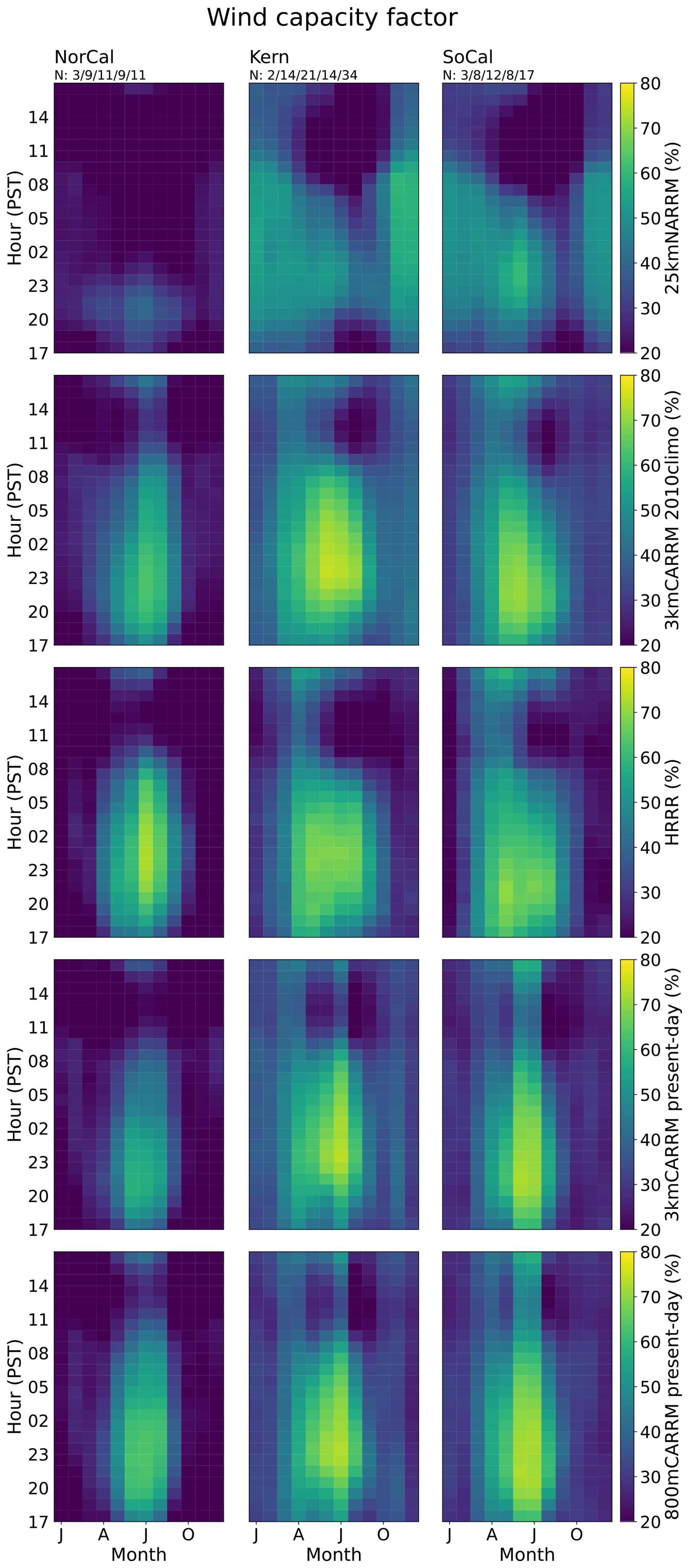
Figure 6 Diurnal and seasonal variation in wind CFs (%) estimated using PySAM. From top to bottom: E3SM-25kmNARRM, SCREAM-3kmCARRM 2010climo, HRRR, SCREAM-3kmCARRM present-day, and SCREAM-800mCARRM present-day simulations, respectively. Each subplot corresponds to a cluster in Fig. 2.

First, all simulations exhibit highly consistent diurnal cycles, with higher values at night and lower during the day. E3SM-25kmNARRM appears highly anomalous, mainly due to the previously discussed seasonal phase reversal and significantly underestimated summer generation. Nevertheless, its diurnal timing remains relatively consistent with the other simulations. All models’ simulated peak values occur at approximately 21:00–24:00 PST, while minimum values occur near 12:00–13:00 PST. Second, in the two comparisons with similar internal variability, diurnal cycle differences are substantially smaller than seasonal cycle differences. The seasonal cycles in Fig. 6 represent an alternate visualization of those in Figs. 3–5.

Overall, the inter-model differences in the diurnal cycle of wind power generation are smaller than the differences between regions (i.e., between northern and southern regions). The wind generation peak period in NorCal, located in north-central California, is slightly shorter than observed in the southern regions of Kern and SoCal.

3.3.5 Statewide wind CFs and meteorological factors

Figure 7 shows the spatial distribution of wind energy resources throughout California. Overall, the best wind resources are found near mountainous regions (e.g., the coastal ranges near the Bay Area, the southern Sierra Nevada, and the eastern highlands of California), where wind CFs generally reach about 50 %. Spatial variability is most pronounced in summer, with the lowest values in areas such as the Central Valley, which maintains the lowest CF year-round, while the highest-value regions reach their seasonal peak. This figure highlights an intuitive but crucial point: wind CF is strongly dependent on local topographic features, and existing wind plants are largely situated in the most resource-rich regions.

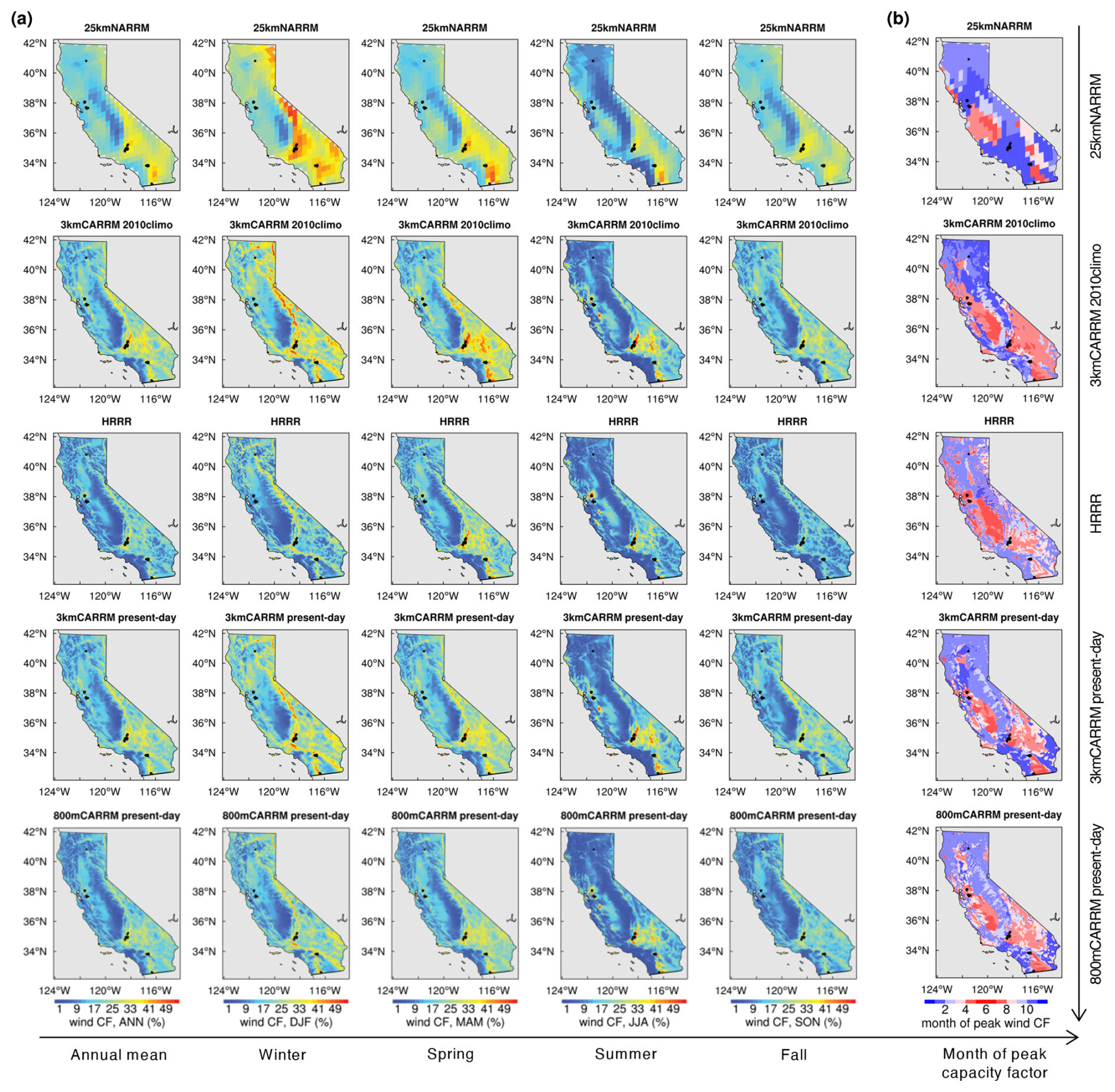
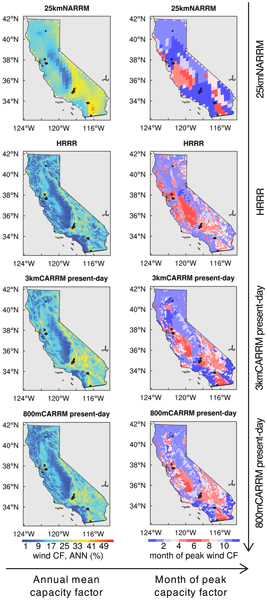
Figure 7 Statewide spatial distribution of (a) wind CFs (%) for California estimated using PySAM, and (b) the month of peak CF. From left to right: annual mean (ANN), winter (DJF), spring (MAM), summer (JJA), and fall (SON) wind CFs, and the corresponding month of peak CF. From top to bottom: E3SM-25kmNARRM, SCREAM-3kmCARRM 2010climo, HRRR, SCREAM-3kmCARRM present-day, and SCREAM-800mCARRM present-day simulations. Valid EIA plant locations are indicated by small black dots on the map.

Figure 7 also shows the month of peak CF in California. First, all km-scale models predict broadly consistent seasonal peaks in wind generation across the state: generally higher in winter and lower in summer in mountainous regions, and the opposite pattern in the coast, the Central Valley, and the desert highlands on the leeward side of Sierra Nevada. Most existing wind farms exhibit summer peaks, whereas northern California (including the Shasta plant) generally peaks in winter, consistent with the EIA plant-level assessment (Figs. 3–5, A3a). Although present-day simulations predict a smaller extent of summer peaks in the Central Valley than the 2010climo simulation and HRRR forecasts, these differences are unlikely to affect planners, given the area’s overall weak wind resource. The seasonal diversity of peak wind generation across California may be advantageous for planners in balancing the supply and demand of different renewable resources, especially given that solar resources are systematically greater in summer. Notably, seasonal peak reversals can occur over short distances, such as winter peaks along the coastline and summer peaks in the adjacent Coast Ranges.

Consistent with earlier findings from the EIA, E3SM-25kmNARRM stands out as an outlier, especially in winter when its wind CF is significantly higher than that of other models. Given the strong dependence of wind resources on local topography, resolution and the model’s ability to resolve topography clearly play a role. When zooming into an evaluation region such as Kern County, the higher-resolution models exhibit pronounced spatial heterogeneity within a single county, whereas the 25 km model lacks this spatial detail (Fig. 1c, d).

To better understand the wintertime discrepancy, Fig. 8 focuses on key variables directly influencing winter wind CF, particularly hub-height winds, as well as large-scale circulation. Notably, E3SM-25kmNARRM not only simulates stronger zonal winds over California but also exhibits stronger northerly winds over Southern California. Its winter blocking ridge is less meridionally extended and located farther offshore relative to ERA5, consistent with its hub-height wind bias (i.e., excessive westerly and northerly winds). The ridge pattern in SCREAM-3kmCARRM 2010climo closely resembles that in 25kmNARRM, although it extends further over land (Fig. 8c). If biases in large-scale circulation were the dominant cause of the winter wind bias, the 3 km simulation would be expected to exhibit similarly large errors, which it does not: 3kmCARRM produces much more realistic wind CFs. In contrast, the SCREAM-CARRM present-day simulations exhibit a stronger ridge than ERA5, while the 2010climo simulation is closer in ridge strength, with the present-day simulations also, somewhat unexpectedly, better capturing the ridge’s position and structure. However, despite these differences in large-scale circulation, the present-day simulations produce wind CF patterns similar to those of the 2010climo simulation. Together, these comparisons suggest that large-scale circulation is unlikely to be the primary driver of wind CF biases, while resolution and topographic representation play a more dominant role.

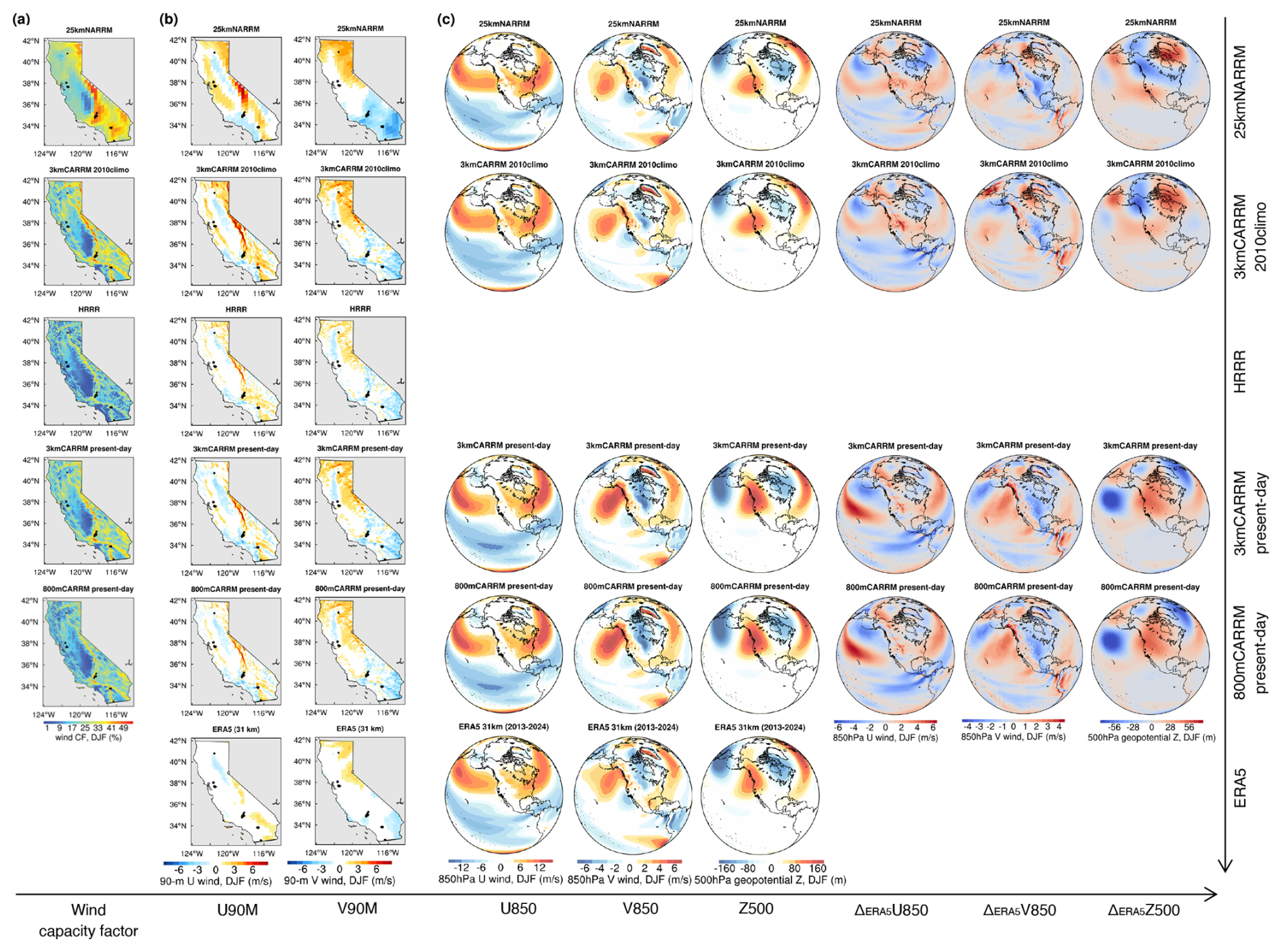
Figure 8 Direct meteorological drivers of wind CFs in winter. From left to right: (a) wind CFs; (b) 90 m zonal winds (U90M) and 90 m meridional winds (V90M), representing hub-height winds; and (c) 850 hPa zonal winds (U850), 850 hPa meridional winds (V850), and 500 hPa geopotential height with the zonal mean removed (Z500), together with the differences between each model-simulated U850, V850, and Z500 and those from ERA5. All quantities are wintertime averages. From top to bottom: E3SM-25kmNARRM, SCREAM-3kmCARRM 2010climo, HRRR, SCREAM-3kmCARRM present-day, SCREAM-800mCARRM present-day simulations, and ERA5. Because ERA5 provides wind output only at 100 m height, the 100 m winds are used as hub-height winds for ERA5. Global U850, V850, and Z500 are not available from HRRR because it is a regional model and does not cover the global domain.

3.3.6 Overall absolute differences in wind energy generation

Figure 9 summarizes the overall discrepancy in simulated wind CFs using the mean absolute bias relative to EIA in the plant-aggregated climatology as the metric, corresponding to the seasonal cycle figures (Figs. 4, 5).

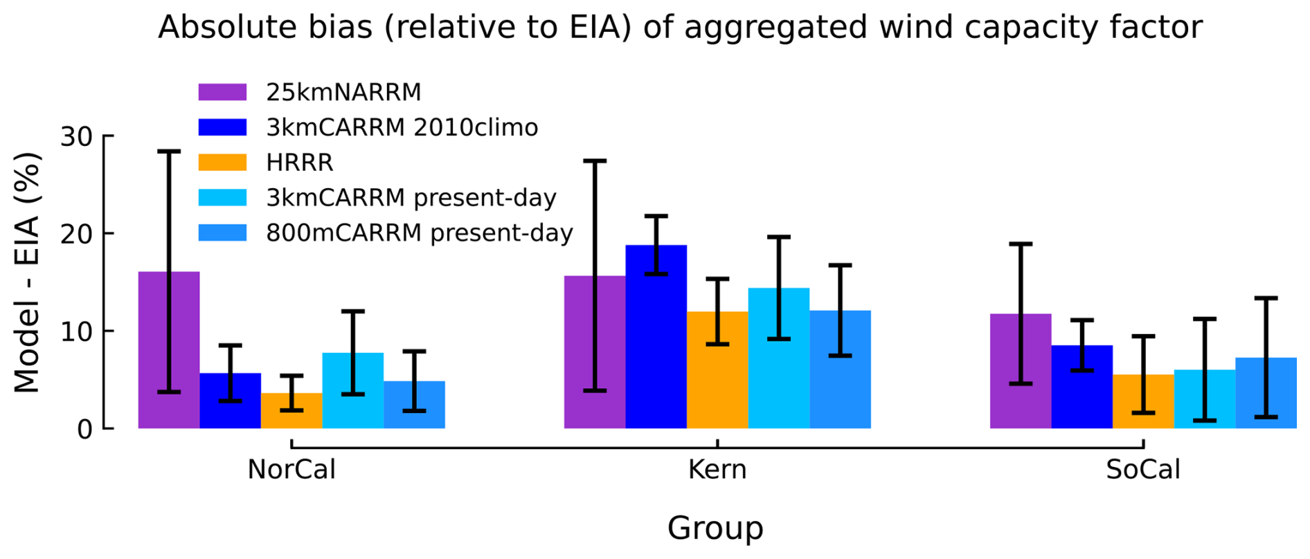
Figure 9 Absolute bias (relative to EIA) of multi-year, plant-aggregated wind CFs (%) from PySAM simulations: E3SM-25kmNARRM (darkorchid), SCREAM-3kmCARRM 2010climo (blue), HRRR (orange), SCREAM-3kmCARRM present-day (deepskyblue), and SCREAM-800mCARRM present-day (dodgerblue). Bar heights indicate the mean absolute bias averaged over the climatological monthly cycle, and error bars denote the standard deviation.

For all clusters, HRRR shows the lowest discrepancy. The 25 km NARRM simulation exhibits the largest discrepancies in the NorCal and SoCal clusters. Notably, SCREAM-3kmCARRM 2010 climo shows the largest mean absolute difference in Kern County; however, its variability is much smaller than that of 25kmNARRM. This reflects the pronounced wintertime discrepancy in 25kmNARRM, as seen in the seasonal cycle (Fig. 5). The SCREAM-800mCARRM simulation produces smaller differences than SCREAM-3kmCARRM in the NorCal and Kern clusters, but larger differences in SoCal.

Overall, differences in annual-mean CF remain within 12 pp, with the vast majority under 2 pp, indicating that the choice of meteorological model has a small impact on time-averaged wind power generation estimates, particularly among the km-scale simulations. At the monthly scale, discrepancies between 25kmNARRM and the km-scale simulations can reach 20 pp in NorCal (Fig. 5).

3.4 Solar

For solar energy, we did not apply the geographic clustering. Instead, we grouped all plants by tracker configuration: single-axis, fixed-axis, and dual-axis. Unlike wind, solar is more uniformly distributed, and hence no natural regional classification emerges. Figure 10 shows the PV plants after aggregating the EIA plants to the 3.25 km CARRM grid.

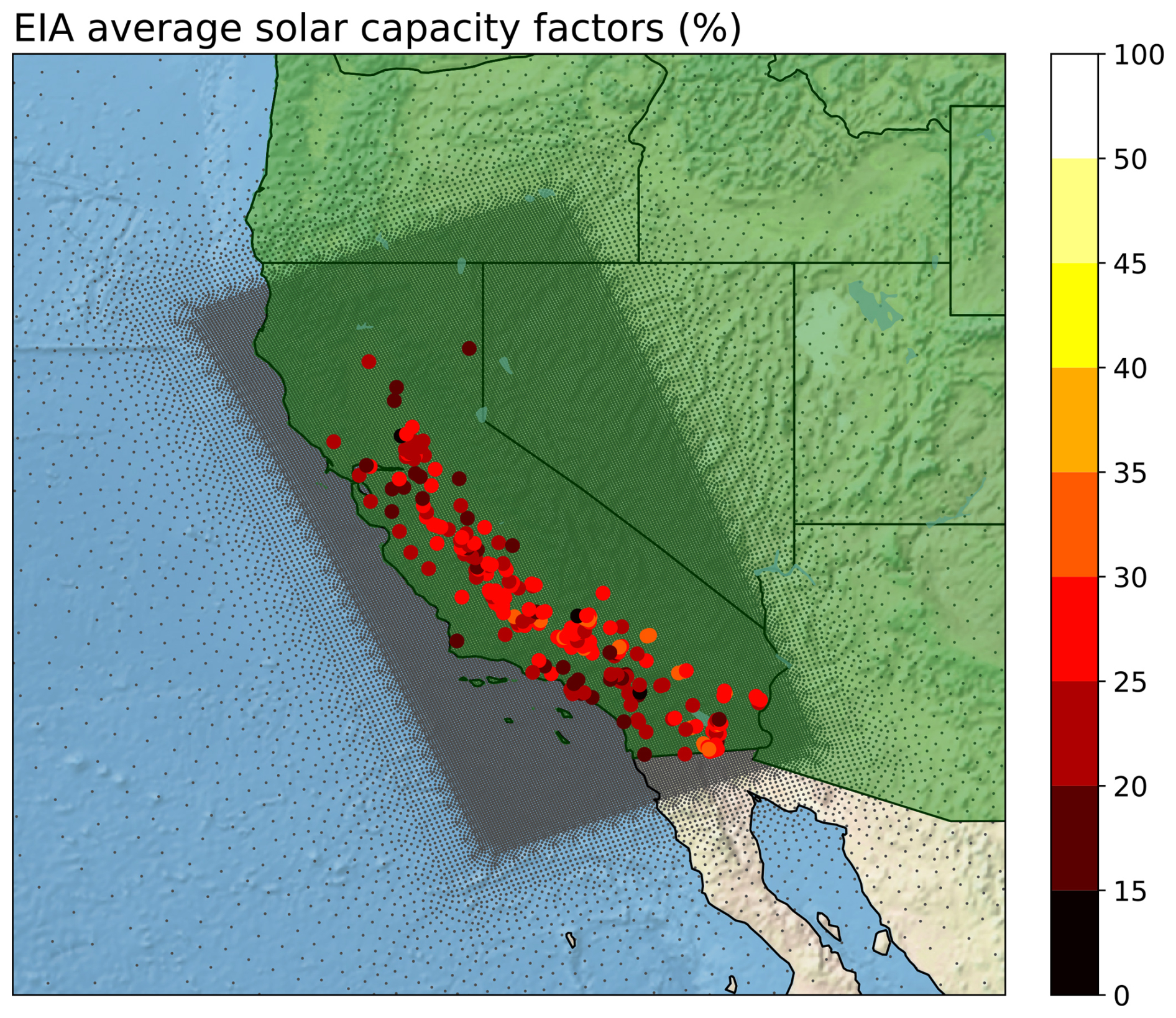
Figure 10 Geographic distribution of solar plants in California. EIA plants are aggregated to the 3kmCARRM model grid; each filled dot represents the mean solar CF (%) from valid monthly EIA records between 2013 and 2024.

As outlined in the Methods section, PV systems are classified by tracker configuration into three categories based on the EIA records: fixed-axis, single-axis, and dual-axis. Fixed-axis arrays are expected to deliver the lowest energy yield, whereas single- and dual-axis trackers adjust panel orientation along one or two axes to follow the sun’s trajectory, keeping the modules closer to normal incidence and thus systematically producing more electricity than fixed-axis systems.

3.4.1 How do different axis-tracking methods affect solar CFs?

Figure 11 shows the solar CFs in California as estimated by PySAM, using SCREAM-3kmCARRM 2010climo and HRRR simulations. Compared to wind, the seasonal cycle of solar CFs is much simpler, with a clear summer peak and winter minimum. Even for dual-axis systems, despite having only three samples, the seasonal pattern remains smooth. This likely reflects the relatively stable solar resource in California’s sunny climate; in cloudier regions with higher solar variability, such smoothness may not hold.

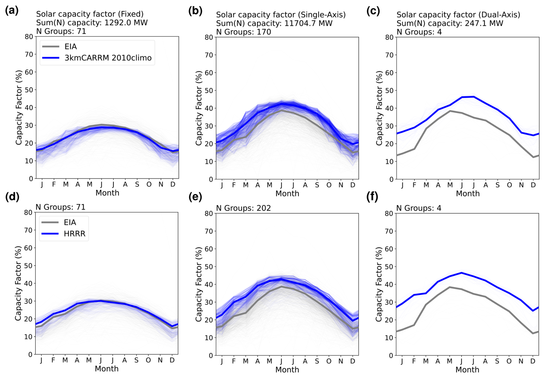
Figure 11 As in Fig. 4, but for solar CFs grouped by tracking type: (a, d) fixed-axis, (b, e) single-axis, and (c, f) dual-axis.

Across the three tracker classes, the overestimation of simulated solar CFs relative to EIA records increases with tracker complexity. For fixed-axis arrays, both SCREAM-3kmCARRM 2010climo and HRRR reproduce the observations well: on average, 3kmCARRM deviates by less than 3 pp in every month. For single-axis systems, the overestimation in both models remains below 6 pp, while for dual-axis systems it stays below 13 pp.

This monotonic increase suggests that the tracker algorithms implemented in PySAM are somewhat idealized. Solar tracking systems are designed to increase energy production by maintaining the panel orientation close to perpendicular to the incoming solar radiation. In principle, dual-axis trackers should therefore achieve higher efficiency than single-axis systems. However, this pattern is not evident in the EIA generation records. One possible reason is that dual-axis systems are mechanically more complex, and operational constraints associated with the control and driving mechanisms may offset part of the theoretical energy gain. In addition, the benefit of multi-axis tracking may be limited in hot climates, where the increased incident irradiance can raise module temperatures and reduce PV output due to thermal losses (El Hammoumi et al., 2022).

In the SAM PV model, tracker orientation follows geometric tracking algorithms that determine panel tilt and azimuth from solar position and array geometry: for single-axis systems, the panel azimuth tracks the solar azimuth while the tilt remains fixed relative to the rotation axis, whereas for dual-axis systems both tilt and azimuth follow the solar zenith and azimuth angles, respectively (Gilman et al., 2018). In practice, mechanical constraints, tracking control strategies, and stow conditions can lead to slower or less precise tracking, reducing the realized energy gains relative to these idealized simulations.

3.4.2 How different are solar CFs between SCREAM-3kmCARRM and HRRR at comparable horizontal resolution?

Figure 11 also compares solar CFs derived from SCREAM-3kmCARRM 2010climo and HRRR simulations. Overall, the two models produce broadly similar seasonal cycles and magnitudes of solar CFs across the three tracker categories.

Some systematic differences nevertheless emerge. Notably, SCREAM-3kmCARRM 2010climo performs remarkably well in reproducing EIA-recorded solar power generation, even outperforming the high-frequency-assimilated HRRR simulation in some months. For fixed-axis systems, the overestimation in HRRR is more pronounced before July: SCREAM-3kmCARRM differs from EIA by about −1 to 1 pp, whereas HRRR shows larger positive differences of roughly 1–2 pp. For single-axis systems, positive discrepancies in SCREAM-3kmCARRM during autumn are slightly more evident than in HRRR, whereas before June they are smaller than in HRRR.

Agreement in energy output alone does not necessarily imply accurate meteorological modeling, since uncertainties in generation modeling (such as the representation of axis tracking, as discussed in the previous section) are difficult to quantify and the reliability of EIA monthly records is not well characterized. Nevertheless, variations in the simulated meteorological drivers of solar power generation likely contribute to the CF discrepancies between the models. Surface downwelling shortwave radiation is the primary determinant of solar CF, and cloud representation can therefore lead to systematic differences in CF. As shown in Sect. 3.4.5, SCREAM exhibits smaller deviations from ERA5 than HRRR in simulating surface solar radiation.

In addition, although this section focuses on CF evaluation, we examined the corresponding meteorological variables in ERA5 over the same period as HRRR (2018–2022) and found spatial patterns very similar to the 2013–2024 climatology (shown in Sect. 3.4.5). This suggests that HRRR solar CFs averaged over 2018–2022 would likely be comparable to those averaged over the EIA record period, implying that the differences identified here primarily reflect differences between meteorological models rather than sampling effects. However, given the many structural differences between the two models, this evaluation quantifies the magnitude of differences in simulated solar CFs but cannot isolate specific causal mechanisms.

3.4.3 How much does horizontal resolution affect solar energy?

Figure 12 shows comparisons that help to understand the impact of resolution on solar energy simulations.

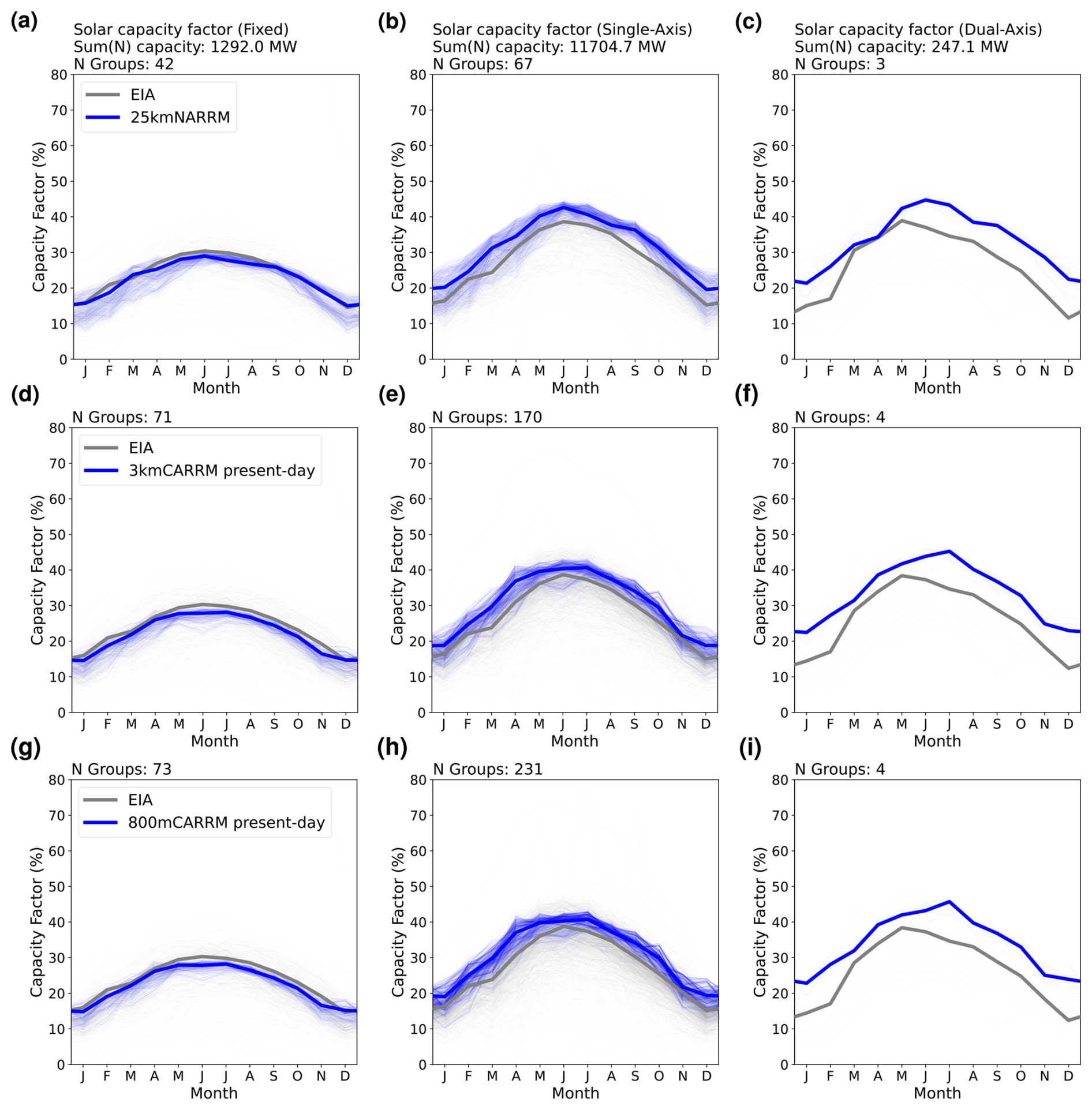
Figure 12 As in Fig. 11 but comparing (a–c) E3SM-25kmNARRM simulations with (d–f) 3.25 km and (g–i) 800 m SCREAM-CARRM present-day simulations.

First, the dominant influence of axis-tracking configuration remains evident here: plants equipped with tracking systems (single- or dual-axis) generally produce more solar energy than those without tracking. In contrast, the influence of spatial resolution appears relatively small in this context. For fixed-axis systems, all three simulations show a slight underestimation relative to the EIA records, with 25kmNARRM exhibiting a smaller discrepancy than the 3.25 km and 800 m CARRM simulations. For single- and dual-axis systems, all simulations show an overestimation, and among single-axis systems the overestimation is most pronounced in 25kmNARRM. As will be shown in the next section on the diurnal cycle, the solar CF simulated by 25kmNARRM reaches particularly high daily peak values, where it is not only higher than in the 3.25 km and 800 m CARRM simulations but even exceeds that of HRRR.

Overall, for solar CFs, the differences between the 25 km and km-scale simulations are less pronounced than those observed for wind CFs. Horizontal resolution therefore does not appear to be the dominant factor controlling inter-model differences, although several notable discrepancies remain. Nevertheless, in cloudier climates, resolution may play a larger role by more accurately capturing sub-grid cloud structures that affect irradiance.

3.4.4 Diurnal cycle of simulated solar power generation

The simulated diurnal cycle of solar CFs is shown in Fig. 13.

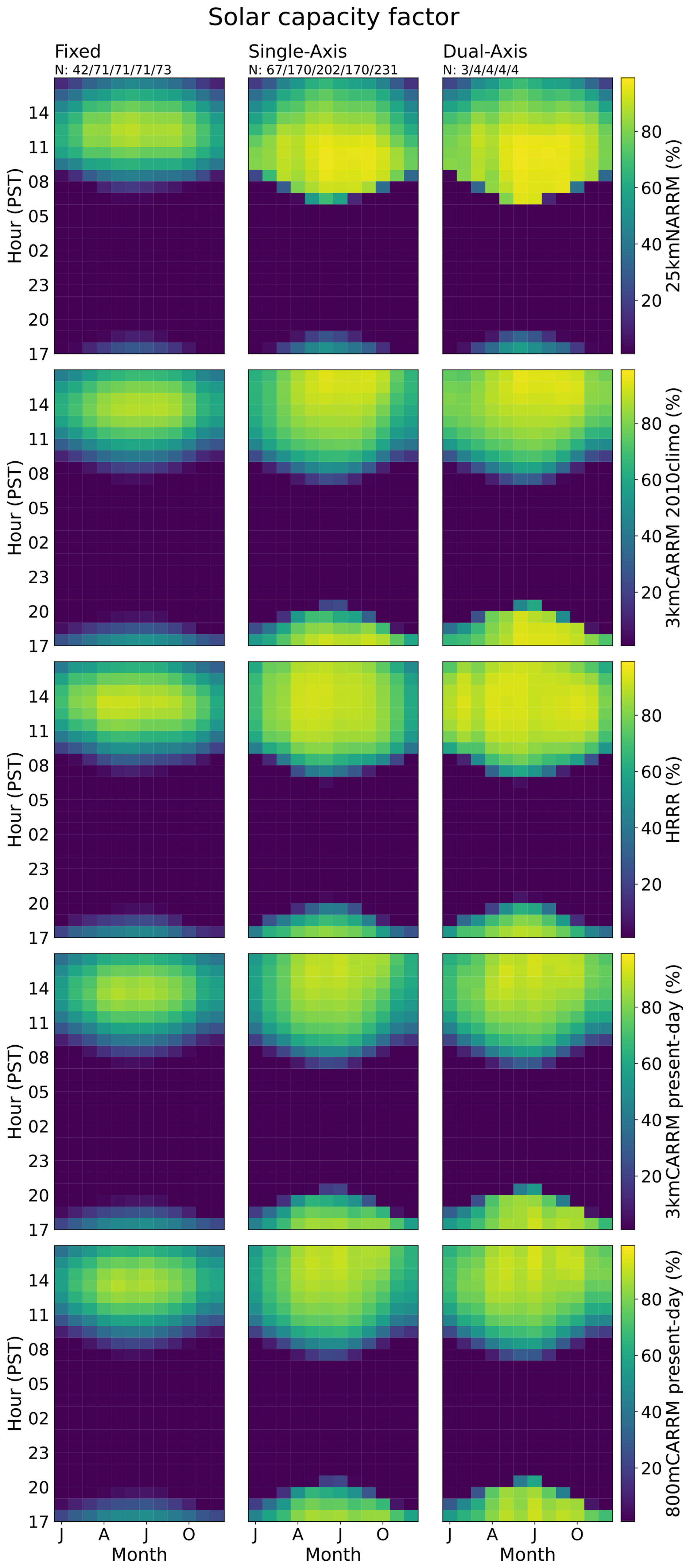
Figure 13 Diurnal and seasonal variation in solar CFs (%) estimated using PySAM. From top to bottom: E3SM-25kmNARRM, SCREAM-3kmCARRM 2010climo, HRRR, SCREAM-3kmCARRM present-day, and SCREAM-800mCARRM present-day simulations. Each subplot corresponds to clusters of fixed, single- and dual-axis tracking.

First, the diurnal pattern of PV generation and its seasonal variation appears to closely match the clear-sky downwelling solar radiation, reflecting the diurnal evolution of solar azimuth angle and the seasonal evolution of solar zenith angle. Both the diurnal cycle and its seasonal dependence show little inter-model or regional variation. For example, the peak solar CF consistently occurs in the afternoon, and the timing of this peak remains nearly unchanged throughout the year across all months.

In terms of magnitude, the km-scale simulations exhibit differences similar to those seen in the seasonal analysis: HRRR generally produces higher solar CFs than all SCREAM-CARRM simulations. The 25kmNARRM simulation stands out for single- and dual-axis tracking in this figure, with extremely high solar CF peaks. Its peak values are not only higher than those of the km-scale SCREAM-CARRMs but even exceed the peak values simulated by HRRR. In addition, for the single-axis and dual-axis categories in 25kmNARRM, PV generation increases very abruptly from near zero to peak values, and the duration of high output is shorter than in the other simulations. For example, in 25kmNARRM during May–July, generation rises from nearly zero at around 06:00 PST to near peak levels by about 08:00 PST, remains high until around noon, and then begins to decrease. In contrast, in all CARRM simulations the increase after 07:00 PST is much more gradual, reaching peak values around 14:00–15:00 PST, followed by a gradual decline until about 20:00 PST. The diurnal amplitude of HRRR during the midday-to-evening decline is very similar to that of the CARRMs, while the morning ramp-up is neither as steep as in 25kmNARRM nor as gradual as in the CARRMs, lying between the two. The HRRR peak hour also occurs slightly earlier than in the CARRM simulations. Overall, however, the diurnal patterns among the km-scale simulations remain broadly similar.

This section provides an additional perspective to the seasonal analysis and again shows that HRRR and 25kmNARRM tend to produce higher solar CFs than the CARRM simulations, although several additional details emerge. In particular, the diurnal cycle in 25kmNARRM is the steepest, especially during the morning ramp-up toward the peak. However, when averaged over the full day, the differences appear less pronounced in the seasonal analysis than in the peak comparisons, because the rapid increase is followed by a similarly rapid decline, resulting in a relatively short duration of high output. The peak timing also differs, with 25kmNARRM reaching peak generation much earlier than the km-scale simulations. Rapid ramps in PV generation pose significant challenges for power system operation, making accurate simulation of the diurnal cycle particularly important (e.g., Ellis et al., 2021; Tarroja et al., 2013).

3.4.5 Statewide solar CFs and meteorological factors

Figure 14 shows the spatial distribution of solar CFs across California. Because the state is dominated by clear-sky conditions, solar CFs are much more spatially homogeneous than wind CFs, generally decreasing from south to north in latitudinal bands. In winter, the northernmost part of California has the lowest CFs, around 9 %, while in summer, most regions reach 25 %–30 %.

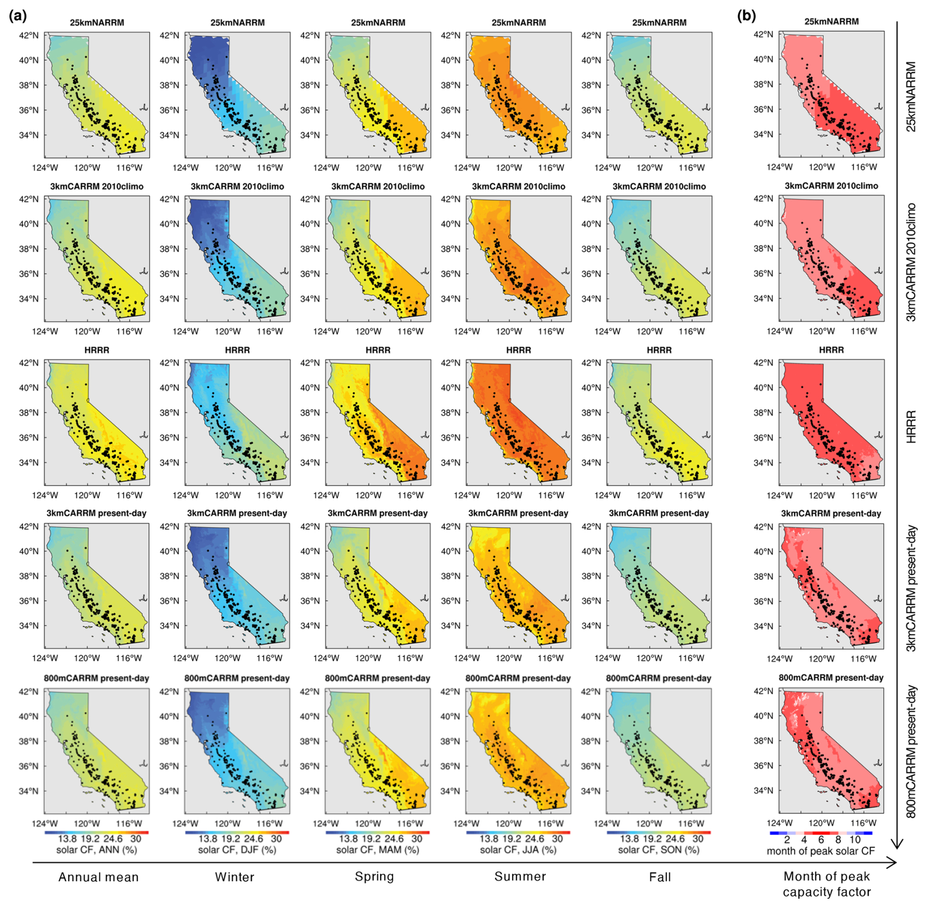
Figure 14 As in Fig. 7, but for solar CFs using the fixed-axis tracking assumption.

Among all simulations, HRRR stands out, consistently producing higher solar CFs than all SCREAM/E3SM RRM simulations evaluated here (Fig. 14). Moreover, HRRR simulates larger amounts of surface downwelling shortwave radiation (Fig. 15). This likely explains why HRRR deviates more from EIA observations than the SCREAM-CARRM simulations, as surface shortwave radiation is the dominant meteorological driver of PV generation. It determines the amount of solar energy collected by PV modules and, together with near-surface air temperature, influences cell temperature and PV performance (e.g., Mayer and Gróf, 2021; El Hammoumi et al., 2022). Surface radiation is highly sensitive to cloud conditions, and clouds remain one of the largest sources of uncertainty in atmospheric modeling because they depend on multiple interacting physical processes. On the other hand, temperature simulations are relatively consistent across all models.

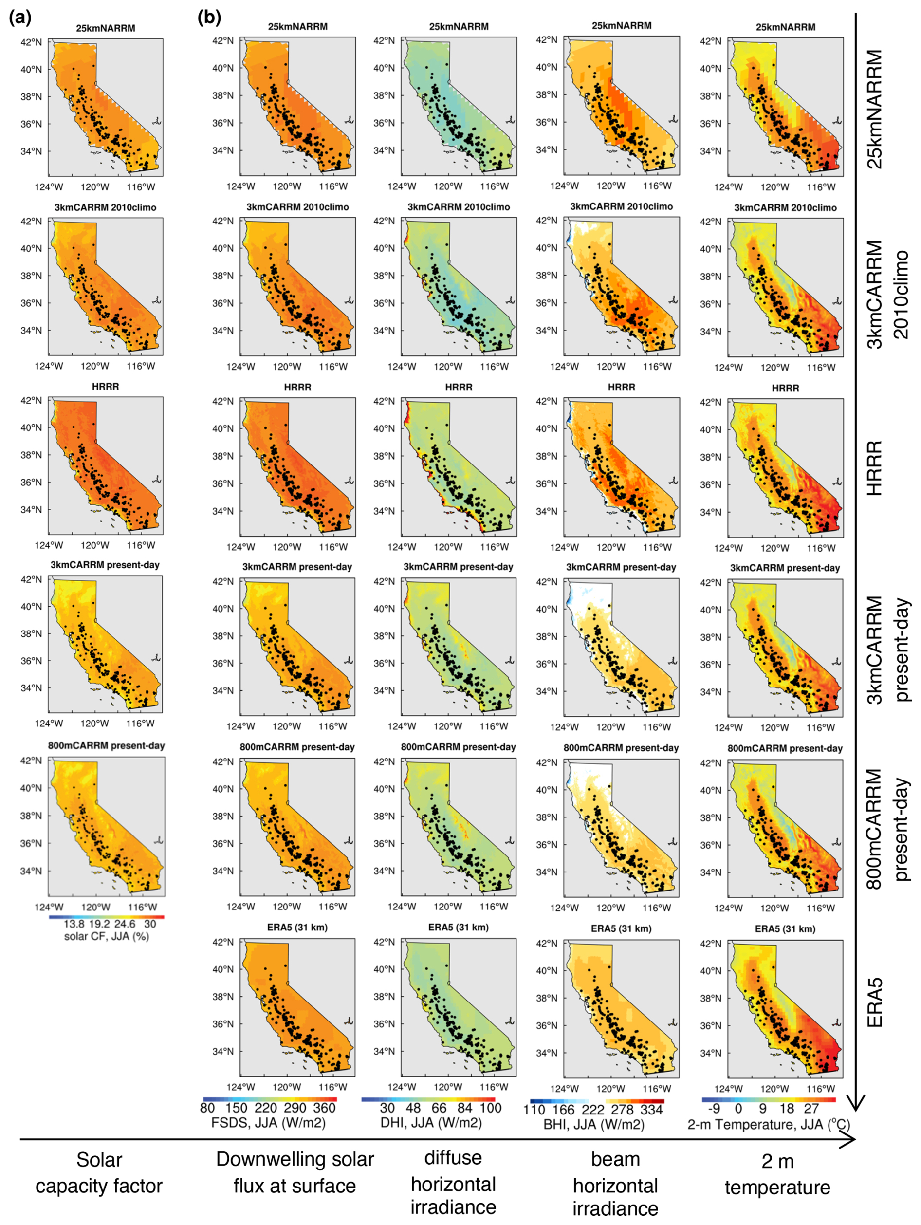
Figure 15 Direct meteorological drivers of summertime solar CFs. From left to right: (a) solar CFs, (b) surface downwelling total shortwave radiation (FSDS), diffuse horizontal irradiance (DHI), beam horizontal irradiance (BHI), and 2 m temperature.

In addition, the spatial distribution of decomposed shortwave radiation components provides further insight. While HRRR produces the strongest total shortwave radiation, the 25kmNARRM simulation shows the second highest values among all simulations. However, its beam component is the strongest over the Central Valley (where EIA stations are densely located), even slightly exceeding that of HRRR. This feature helps explain why the enhancement from fixed to single-axis tracking is strongest in 25kmNARRM, as shown in Fig. 13. Because single-axis tracking allows PV panels to follow the solar azimuth, a higher relative contribution of the beam component leads to a larger increase in PV generation compared to fixed systems.

3.4.6 Overall absolute differences in solar energy generation

Figure 16 presents a summary of discrepancies in simulated solar CFs, quantified using the mean absolute bias relative to EIA in the plant-aggregated climatology. Fixed-axis systems show the smallest discrepancies (all below 2 pp), while single-axis tracking ranges from 4–6 pp, and dual-axis systems exhibit overestimation of 7–10 pp. This pattern suggests a systematic effect: discrepancies increase with tracking complexity. One plausible explanation is that PySAM’s tracking algorithms may idealize real-world performance. Notably, SCREAM-CARRMs show smaller discrepancies than HRRR across all tracking types.

Figure 16 As in Fig. 9 but for solar CFs.

4 Conclusions

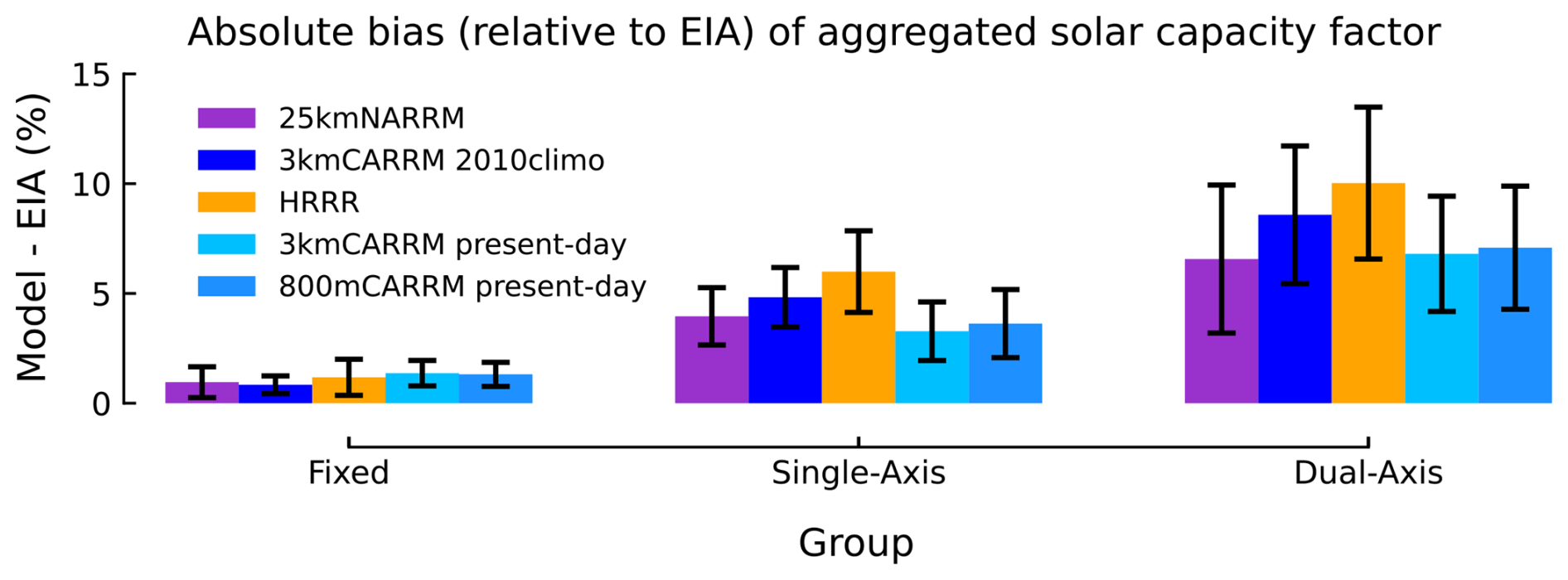
This study evaluates wind and solar power generation derived via PySAM from SCREAM-CARRMs at 3.25 km and 800 m resolutions, through comparisons with EIA records, PLUSWIND, and HRRR. The following summarizes our responses to the three central questions raised in the Introduction:

1. Does the use of different energy models affect wind CFs? How do different axis-tracking methods affect solar CFs? For wind, the choice of generation model (PySAM vs. PLUSWIND) introduces larger differences than variations in results due to internal assumptions within PLUSWIND (e.g., air density or loss treatments), but still smaller than discrepancies caused by differing meteorological models (Fig. 3). For solar, however, axis tracking plays a major role (Fig. 11). As seen in Fig. 16, discrepancies increase with tracking complexity, suggesting that PySAM’s idealized tracking assumptions may not fully reflect the mechanical or operational limitations of real-world systems.

2. How different are wind and solar CFs between SCREAM-3kmCARRM and HRRR at comparable horizontal resolution? Despite being based on two fundamentally different meteorological models, both SCREAM-3kmCARRM 2010climo and HRRR produce similar wind and solar generation when processed with PySAM: the annual-mean plant-aggregated climatology differs by 2–7 pp for wind and 0.3–3 pp for solar (Figs. 9, 16). While HRRR differs less from EIA data for wind, SCREAM-3kmCARRM aligns more closely for solar generation.

3. How much does horizontal resolution affect wind and solar energy calculations? The transition from E3SM-25kmNARRM to SCREAM-3kmCARRM results in a performance leap for wind energy, particularly in capturing the seasonal cycle (Fig. 5), highlighting the importance of improved horizontal resolution and better representation of topography. In contrast, the difference between the 3.25 km and 800 m SCREAM-CARRM present-day simulations (and E3SM-3kmCARRM and HRRR from bullet 2) is minimal, with annual-mean plant-aggregated climatology differing by 1–4 pp (Fig. 9), indicating limited resolution sensitivity at these finer scales in SCREAM. Solar PV generation shows much lower resolution sensitivity across E3SM-25kmNARRM, 3.25 km SCREAM-CARRM, and 800 m SCREAM-CARRM than the differences between SCREAM and HRRR (Fig. 16).

It should be noted that absolute bias alone cannot fully characterize differences in model performance, as it does not capture phase errors in the seasonal cycle and does not allow clear attribution of EIA-model differences to the model alone, given uncertainties in both the observational data and the modeling framework. In the absence of hub-height wind observations, detailed solar radiation measurements (total and beam/diffuse), and hourly EIA data, the sources of EIA-model differences cannot be precisely attributed. Although the contribution of meteorological forcing errors remains uncertain, comparisons across the three questions provide insight into the relative influence of different factors on modeled generation.

The importance of resolution for wind energy is supported by findings from PLUSWIND and by our comparison between 25kmNARRM, 3kmCARRM, and 800mCARRM, where the seasonal phase mismatch previously identified in NARRM is no longer present in CARRMs, underscoring the improvements gained through km-scale modeling. This has critical implications for power system planning, as seasonal variability plays a key role in balancing supply and demand, and its uncertainty cannot be effectively mitigated by short-duration storage technologies such as batteries (e.g., Staadecker et al., 2024). The conclusion that km-scale simulations perform substantially better than O(10 km) simulations for wind power generation is likely applicable to other regions with complex terrain, as topography is one of the most dominant lower boundary conditions controlling winds. However, increasing the resolution from 3.25 km to 800 m adds little value to SCREAM’s wind generation, given the ∼ 45× increase in computational cost. In particular, the seasonal pattern shows that while the 800 m simulation reduces wintertime overestimation, it amplifies summertime overestimation. Nevertheless, this climatological evaluation does not necessarily extend to high-frequency applications (e.g., hourly operational power flow simulations), where higher resolution could still be beneficial.

Regarding the lack of large sensitivity between 3.25 km and 800 m SCREAM-RRMs, this likely depends on SCREAM’s turbulence scheme and may not necessarily generalize to other models. SCREAM’s SHOC turbulence scheme is scale-aware and scale-insensitive, meaning that a larger fraction of turbulent kinetic energy is explicitly resolved as resolution increases, while the representation of clouds and thermodynamics does not change substantially with resolution (Bogenschutz et al., 2023). Turbulence schemes lacking this property, which are generally used in coarser GCMs, may artificially exaggerate the contribution of subgrid transport at 800 m resolution. On the other hand, the muted sensitivity may also be attributed in part to model errors associated with the turbulence gray zone (e.g., Wyngaard, 2004; Chow et al., 2019; Honnert et al., 2020); see also discussions in Zhang et al. (2026). Specifically, horizontal turbulent mixing (neglected in most PBL schemes including SHOC) may become non-negligible at 800 m, especially in complex terrain where three-dimensional effects matter (e.g., Juliano et al., 2022; Arthur et al., 2025b).

The comparison between SCREAM-3kmCARRM and HRRR suggests that structural differences in the meteorological models have less impact on generation estimates than horizontal resolution. The more pronounced wintertime overestimation of wind generation by SCREAM compared to HRRR may indicate a systematic seasonal bias in SCREAM-CARRMs’ wind simulations. This can be partially explained by the less meridionally extended high-pressure blocking ridges in the 2010climo simulation, which tend to favor an overestimated frequency of atmospheric rivers and associated cold-front winds.

For generation modeling, PySAM applied to HRRR produces wind generation estimates closer to EIA and with less overestimation than PLUSWIND, suggesting that loss estimation may be the dominant factor. Although PLUSWIND’s turbine power curve derived from plant-level turbine diameter and capacity is theoretically more accurate than PySAM’s default curve, its assumed ∼ 7 % loss factor (Millstein et al., 2023) may be underestimated, based on the comparison between HRRR+PySAM and HRRR+PLUSWIND. In addition, we provide PySAM with each model’s own hourly temperature, humidity, and pressure fields to calculate air density, ensuring consistency with the wind inputs. In contrast, PLUSWIND uses the same MERRA2-based air density estimates even when driven by high-resolution wind fields like HRRR, potentially introducing a resolution mismatch.

For the comparison between solar CFs simulated by 3kmCARRM and 25kmNARRM, the conclusion that PV power generation is relatively insensitive to horizontal resolution may partly reflect California’s predominantly clear-sky conditions, under which model biases are muted, and may therefore be limited to regions where mesoscale cloud-precipitating processes are not prevalent. Although California contains extensive mountain ranges, precipitation is primarily associated with large-scale systems (atmospheric rivers) and is relatively infrequent overall, particularly during summer when solar generation is at its peak. Local orographically forced precipitation and mesoscale convective systems are largely absent.

The smaller solar CF discrepancies between SCREAM-CARRMs and EIA, relative to HRRR, are consistent with their smaller bias in surface shortwave radiation, highlighting SCREAM’s potential applicability in regions with similar climates. Sensitivity to different meteorological models may also be broadly applicable, since the representation of clouds (especially low clouds) remains one of the largest sources of uncertainty in atmospheric models.

For PV generation modeling, axis-tracking type remains the dominant source of variation, with discrepancies increasing alongside tracking complexity. This suggests that PySAM’s multi-axis tracking assumptions may be overly idealized compared to real-world system behavior. The sensitivity of PV generation to axis tracking is primarily governed by the geometric configuration of PV panels and is therefore expected to be robust. However, it remains unclear whether the overestimation of multi-axis tracking identified in PySAM reflects a general modeling issue or is specific to that model.

Several limitations of this study are worth noting. First, although the EIA monthly data represent the best available “observations” they are not automatically collected, and the quality-control procedures used to derive monthly total generation are unclear; imputation introduces an additional concern. As a result, we cannot disentangle the impacts of data processing or operational losses, such as outages and curtailment, nor can we fully avoid the effects of imputation, which would otherwise substantially reduce the effective sample size and damp the spread of interannual variability. Second, none of the E3SM/SCREAM simulations conducted here are weather hindcasts, i.e., the simulated time series do not correspond one-to-one with historical observations. Thus, our evaluation is limited to climatological statistics rather than specific time series or historical events. Finally, we did not conduct an extensive sensitivity analysis and instead chose to follow the default assumptions of PySAM, as detailed plant-level optimization of the energy model is not the primary focus of this work.

Overall, this work demonstrates the importance of high-resolution simulations for wind and solar estimates and that SCREAM-RRM is a viable tool for such energy resource assessments. With improved observational constraints and efforts to better quantify generation modeling uncertainties, future work can further understand SCREAM’s biases and apply SCREAM to long-term power generation prediction and optimization.

Appendix A: Applying an independent-plant ratio threshold to EIA monthly data

During our analysis, we encountered a puzzling phenomenon: for all simulations, the seasonal cycle of the Shasta CF (2013–2024 climatology) was completely out of phase with the multi-year mean seasonal cycle recorded in the EIA data. This plant was so unusual because no other plant in the km-scale simulations exhibited such an off-seasonal-phase issue. In the absence of nearby wind observations, it was difficult to determine whether all models were wrong or whether the EIA record was wrong.

A key insight came from an anonymous reviewer of Lee et al. (2026), who cautioned:

EIA gathers monthly data from a subset of plants from each state, creates monthly weights for that state, and then, for the rest of the plants in the state, distributes reported annual generation to each month based on the state-level weights… You can observe this in the data if you take the ratio of July to January (or any two months) across a set of plants in a state. Some of the plants will have independent ratios, but many plants will have the exact same July to January ratio. For those plants with non-independent monthly profiles, EIA only gathers annual generation records.

In fact, the EIA-923 documentation (https://www.eia.gov/electricity/monthly/pdf/technotes.pdf, last access: 8 August 2025) briefly describes the imputation method on pages 3 and 15:

Imputation: For monthly data, if the reported values appeared to be in error and the data issue could not be resolved with the respondent, or if the facility was a nonrespondent, a regression methodology is used to impute for the facility. The same procedure is used to estimate (“predict”) data for facilities not in the monthly sample. The regression methodology relies on other data to make estimates for erroneous or missing responses.

Imputation: For select survey data elements collected monthly, regression prediction, or imputation, is done for missing data, including non-sampled units and any non-respondents. For data collected annually, imputation is performed for non-respondents.

To assess the degree of imputation in the annually collected data, and in particular to understand the mysterious behavior of Shasta, we quantified the severity of imputation for each plant and each year.

For the valid EIA plants selected by the aforementioned quality control criteria, we computed the Pearson correlation distance (i.e., 1 minus the Pearson correlation coefficient) for monthly data between every pair of plants for each year. The yearly distances were plotted as scatterplots (Fig. A1). If the distance value was less than 10⁻⁶ (i.e., close to 0, accounting for truncation error), then the plant pair was deemed non-independent. Vertical lines in Fig. A1 indicate that a plant i has an identical correlation coefficient with multiple other plants ($j=\mathrm{1},\mathrm{\dots },N$), implying that the j plants are non-independent and plant i is independent. If in a given year, there were no plant pairs with zero distance and no vertical lines, the year was classified as a fully-independent year, meaning no imputation existed among any plants. Taking wind as an example: in 2017, all plants are non-independent (all scatter points are bright green with no blue vertical lines); in 2013, most plants are independent, but some are non-independent (clusters with distance =0 appear larger in size and are bluer in color); in 2023 and 2024, there are no blue vertical lines and no clusters with distance =0 for wind CFs (all scatter points have the same size), indicating that all plants in that year are independent.

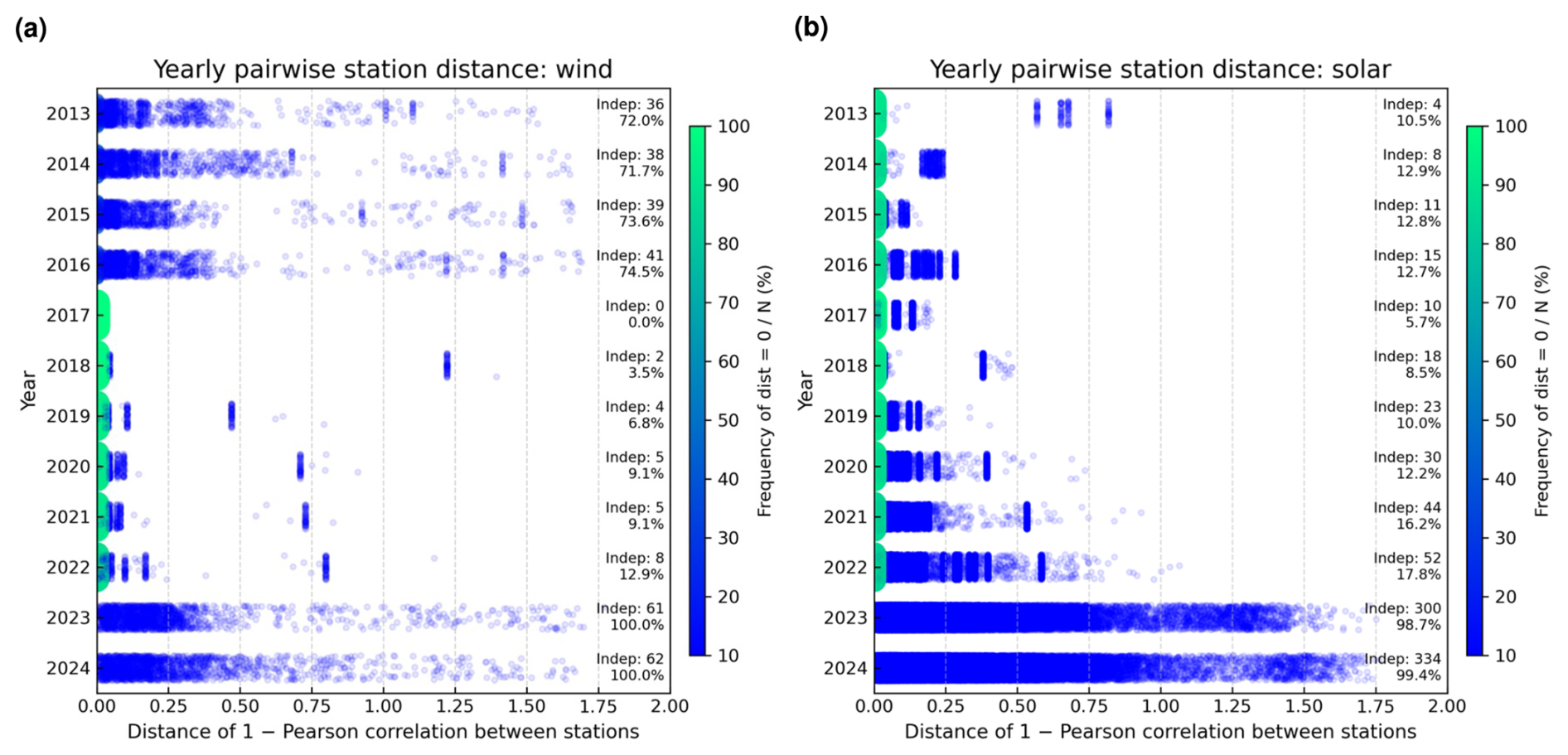
Figure A1 Scatter plots for assessing plant independence for (a) wind and (b) solar. Each point represents the Pearson correlation distance for a given year and plant pair, with the value on the x axis and the year on the y axis. Distances closer to zero (considering a truncation error of 10⁻⁶) are shown in brighter green, and the sizes of the corresponding scatter points are set larger; conversely, larger distances are shown in blue with a constant size. A vertical jitter of ±0.25 is applied to the y axis for each year. This visualization step highlights independent samples: plants that have a fixed Pearson correlation distance with multiple other plants, which appear as short blue vertical lines in the figure. The number of independent plants and their proportion relative to all plants in that year are quantified and displayed as text to the right of each subplot for each year.

From Fig. A1, it can be seen that 2023 and 2024 were the only fully independent years between 2013 and 2024 for wind CFs, and solar CFs in these two years were also nearly fully independent. The degree of imputation (i.e., the proportion of plants whose seasonal cycles are imputed from other plants) varies from year to year: for wind, in 2017–2022, the vast majority of plants (> 90 %) had artificial seasonal cycles, whereas for solar, a large fraction (>80 %) of plants had artificial seasonal cycles starting as early as 2013. To visualize this more directly, Fig. A2 shows Shasta’s independence status for each year from 2013 to 2024: red for independent years, blue for non-independent years, and thin gray lines for other plants.

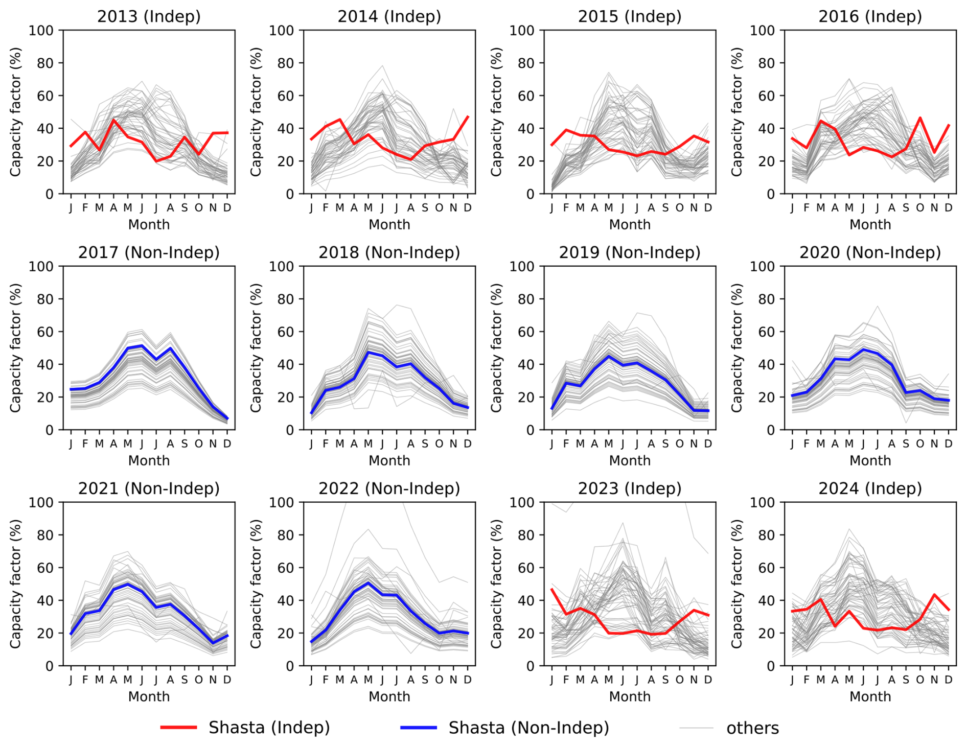
Figure A2 Determination of whether the Shasta plant is independent in each year based on the Pearson correlation distance for each plant pair in that year. When Shasta is independent, it is shown as a thick red line; when non-independent, as a thick blue line. All other valid plants are shown as thin gray lines.

Based on this analysis, we conclude that removing years dominated by plants with imputed data is more appropriate for seasonal pattern analysis. However, removing those years would reduce the sample size for annual-mean discrepancy analysis. Therefore, we set an “independent-plant ratio” threshold of N_independent> 15 %, which leads to the exclusion of the following years: wind: {2017, 2018, 2019, 2020, 2021, 2022}, solar: {2013, 2015, 2017, 2018, 2019}. Figure A3 compares the seasonal cycle of wind and solar CFs before and after applying the “independent-plant ratio > 15 %” threshold. However, this distance-correlation filter cannot be applied to PLUSWIND, as it would remove all available years (2018–2021).

Comparing results with and without this threshold shows that the largest impact is on the Shasta wind plant (Fig. A3a): without the threshold, Shasta exhibits an exactly out-of-phase seasonal cycle between all model simulations and the EIA record; with the threshold applied, this artificial behavior disappears entirely, since 2017–2022 are exactly the years when the Shasta wind CF was imputed from other plants (Fig. A2). This correction also affects northern California, shifting the wind CF peak month from May to July (Fig. A3a), but has little effect on wind in other regions of California or on any PV plants (Fig. A3b).

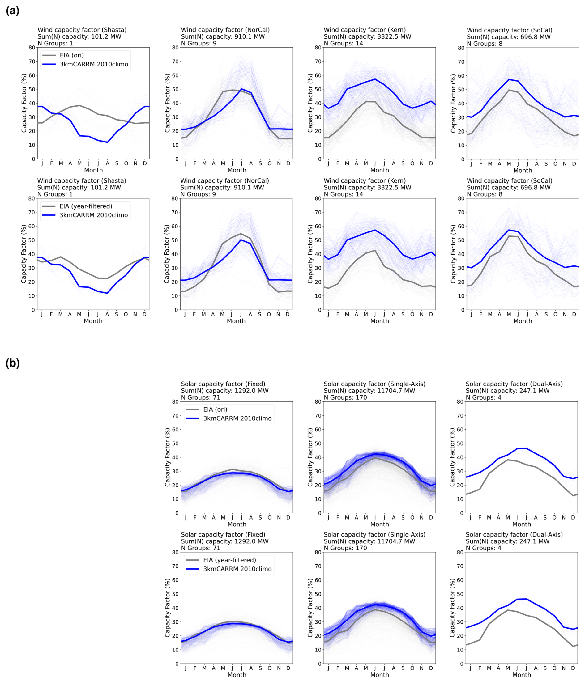
Figure A3 Seasonal variation in the (a) wind and (b) solar CFs (%) estimated using PySAM from SCREAM-3kmCARRM 2010climo, before (upper) and after (bottom) applying the “independent-plant ratio > 15 %” threshold (i.e., excluding years dominated by imputed plant data). The years before filtering are 2013–2024. After filtering, the valid years are {2013, 2014, 2015, 2016, 2023, 2024} for wind and {2014, 2016, 2020, 2021, 2022, 2023, 2024} for solar, respectively. Each column corresponds to a cluster for wind or solar CFs, with Shasta also included here. Simulations are shown in blue, and EIA records in gray. Light lines represent individual years; bold lines represent the multi-year climatology.