the Creative Commons Attribution 4.0 License.
the Creative Commons Attribution 4.0 License.
 | 20 May 2026
Operational chemical weather forecasting with the ECCC online Regional Air Quality Deterministic Prediction System version 023 (RAQDPS023) – Part 1: system description
Verica Savic-Jovcic
Craig A. Stroud
Sylvain Ménard
Wanmin Gong
Junhua Zhang
Qiong Zheng
Jack Chen
Ayodeji Akingunola
Alexandru Lupu
Konstantinos Menelaou
Rodrigo Munoz-Alpizar
The online version of the Regional Air Quality Deterministic Prediction System (RAQDPS) is a chemical weather forecast system that has been employed operationally by Environment and Climate Change Canada (ECCC) since 2009. It is run twice per day to produce 72 h forecasts of hourly 10 km abundance fields of three key predictands, NO2, O3, and PM2.5 total mass, as well as other gas-phase chemical species, PM2.5 chemical components, and dry and wet deposition for Canada, the contiguous U.S., and northern Mexico. The forecasts of NO2, O3, and PM2.5 are needed to calculate the Air Quality Health Index (AQHI), which is used to communicate current and forecasted pollutant levels to the Canadian public. Version 023 of the RAQDPS (RAQDPS023) went into service at ECCC in December 2021 and was replaced by the RAQDPS025 in June 2024. This paper provides the first full description of any version of the online RAQDPS. After giving a brief history of the ECCC operational air quality forecasting program, we provide a comprehensive description of the RAQDPS023 forecast system as well as shorter descriptions of several upstream and downstream forecast and analysis systems. The latter include two upstream operational meteorological forecast systems that were based on version 5.1.0 of the ECCC Global Environmental Multiscale (GEM) numerical weather prediction model, one which used a global configuration, the Global Deterministic Prediction System (GDPS 8.0.0), and the other which used a regional configuration, the Regional Deterministic Prediction System (RDPS 8.0.0). An emissions processing system, an Updateable Model Output Statistics-based system for bias-corrected station-specific pollutant concentration forecasts (UMOS-AQ), and a regional objective analysis system for surface pollutant concentration fields, the Regional Deterministic Air Quality Analysis system (RDAQA 2.0.0), are also described.
The RAQDPS023 itself consisted of version 3.1.0.0 of the GEM-Modelling Air quality and CHemistry (GEM-MACH) chemistry module, which was embedded with one-way coupling within GEM 5.1.0, its meteorological host model. The meteorological configuration of the RAQDPS023 closely followed that of the RDPS 8.0.0. Details covered in this paper include a summary of the dynamical representations and physical parameterizations used in the three GEM-based forecast systems, which are highly harmonized, the chemical species and parameterizations used in the MACH chemistry module, including gas-phase, aqueous-phase, and inorganic heterogeneous schemes and associated numerical solvers, system inputs, including both anthropogenic and natural emissions of chemical species, system outputs, and run configuration, strategies, and timings. One simplification in addition to the use of the condensed ADOM-2 gas-phase chemistry scheme that was made to reduce RAQDPS023 execution time for operational deployment was to represent the particulate matter (PM) size distribution with only two aerosol particle size bins, one corresponding to particle diameters in the 0–2.5 µm range (“fine particles” or PM2.5) and the other to the 2.5–10 µm range (“coarse fraction” or PMcf). A second simplification was to represent the chemical composition of PM2.5 with only nine chemical components, and a third simplification was to use a longer time step (900 s) for the time integration of atmospheric chemistry than the time step used for time integration of atmospheric dynamics and physics (300 s). Even so, activating the MACH module increased RAQDPS023 run time by a factor of 4.4 on average compared to meteorology only, partly due to the cost of the integration of chemistry but partly to the increased cost of the GEM dynamical core due to the advection with imposed shape preservation and mass conservation of 57 additional chemical tracers. The role of the RAQDPS-FW023, a second chemical weather forecast system that was identical to the operational RAQDPS023 (or RAQDPS-OP023) except for the addition of near-real-time biomass burning emissions, is also described. Biomass burning emissions for Canada and the U.S. estimated from satellite measurements were first calculated by the Canadian Forest Fire Emissions Prediction System (CFFEPS) version 4.1 before each RAQDPS-FW023 run was launched. Outputs from the two RAQDPS versions were then used to produce forecasts of wildfire smoke transport and diffusion. The paper closes by summarizing the key upgrades made to the RAQDPS025, the current version of the ECCC operational chemical weather forecast system, and then describing some possible future improvements and updates. A companion paper by Moran et al. (2026) presents the results of a comprehensive, five-year performance evaluation of prospective and retrospective annual air quality simulations made with the RAQDPS023.
- Article
(6240 KB) - Full-text XML
- Companion paper
-
Supplement
(564 KB) - BibTeX
- EndNote


Forecasting tomorrow's weather means being able to predict the short-term future dynamical and physical state of the atmosphere. Operational weather forecasting, also known as numerical weather prediction (NWP), began in the 1950s once electronic computers started to become available commercially (e.g., Lorenz, 2006; Bauer et al., 2015). The chemical state of the atmosphere, on the other hand, particularly the concentrations of air pollutants of concern for human health, is often referred to as air quality (AQ). Recent epidemiological studies have determined that air pollution is the fourth leading cause of early death globally (Boogaard et al., 2019; Murray et al., 2020; WHO, 2021). However, predicting tomorrow's air quality, or chemical weather as it is also known, is even more difficult than predicting tomorrow's weather. As a consequence, operational regional AQ forecasting did not become possible until about 2000 (McHenry et al., 2004; Kukkonen et al., 2012; Zhang et al., 2012a), roughly a half century after the start of operational weather forecasting.
Air quality was initially only a local concern in the vicinity of large sources of air pollutants, including major urban centres (Pasquill and Smith, 1983). In the 1970s, however, emerging recognition of human health impacts caused by regional photochemical smog and the environmental harm caused by regional acidic deposition (or “acid rain”) spurred many laboratory and field studies to better understand these larger-scale AQ issues (e.g., Hecht et al., 1974; Likens and Bormann, 1974; Eliassen and Saltbones, 1975; Barrie and Georgii, 1976; Calvert et al., 1978; Harrison et al., 1978; Schiermeir, 1978). The development of the first prognostic, three-dimensional, regional AQ models capable of simulating photochemical smog, especially ozone, and acidic deposition then followed in the 1980s, building on the steady increase in our scientific understanding of these issues (e.g., Chang et al., 1987; Seinfeld, 1988; Venkatram et al., 1988; Russell and Dennis, 2000). At first these regional AQ models, which are also known as chemical transport models (CTMs) and atmospheric chemistry models (Kukkonen et al., 2012), were only applied to retrospective case studies for research and policy applications (e.g., Clark et al., 1989; Fung et al., 1991; Roselle and Schere, 1995; Dunker et al., 1996; Middleton, 1997). Routine regional AQ forecasting was held back by two factors – the order-of-magnitude larger computational burden of AQ models relative to NWP models and the run-time constraints imposed by the need to disseminate forecasts in a timely fashion (McHenry et al., 2004) – but continuing improvements in computer capabilities have facilitated the introduction and rapid expansion of the use of operational AQ forecast systems in North America, Europe, and Asia over the past two decades (e.g., Grell and Baklanov, 2011; Kukkonen et al., 2012; Zhang et al., 2012a, b; Brasseur et al., 2019; WMO, 2020; Brasseur and Kumar, 2021).
The majority of AQ forecast systems employ a so-called “offline” model architecture, where an NWP model is run first and then a CTM is run using forecast meteorological fields from the NWP model as inputs. More recently, however, some AQ forecast systems have adopted an “online” architecture where meteorological and chemical variables are predicted simultaneously, in effect a merged NWP-CTM system (e.g., Grell et al., 2005; Zhang, 2008; Grell and Baklanov, 2011; Baklanov and Zhang, 2020).
Canada was one of the first countries to implement an operational regional AQ forecast system (e.g., Zhang et al., 2012a). Environment and Climate Change Canada (ECCC), Canada's federal environment ministry, has run an operational, continental-scale Regional Air Quality Deterministic Prediction System (RAQDPS) for North America since 2001. The earliest version of the RAQDPS employed an offline CTM called CHRONOS (Canadian Hemispheric Regional Ozone and NOx System). This system was run once per day on a 21 km horizontal grid over North America with 25 vertical levels from the surface to 6 km to make 48 h forecasts of surface ozone (O3) volume mixing ratio (Pudykiewicz et al., 1997; Pudykiewicz and Koziol, 2001; McHenry et al., 2004; McKeen et al., 2005; Ménard and Robichaud, 2005; Moran et al., 2013; Robichaud and Ménard, 2014). The meteorological “driver” (i.e., NWP model) used with CHRONOS was the limited-area ECCC Regional Deterministic Prediction System (RDPS), the operational, nested, regional configuration of the ECCC Global Environmental Multi-scale (GEM) NWP model (Côté et al., 1998a, b; Fillion et al., 2010; Caron et al., 2015). The surface concentration of particulate matter (PM) with aerodynamic diameter smaller than 2.5 µm (PM2.5) was added as a predictand to CHRONOS in 2003 (Pudykiewicz et al., 2003; McKeen et al., 2007).
In 2009 the offline CHRONOS CTM in the RAQDPS was replaced by the online, one-way-coupled GEM-MACH (GEM–Modeling Air quality and CHemistry) chemical weather model, which included improved representations of gas-phase, aqueous-phase, and aerosol chemistry in the new MACH chemistry module that was added to the GEM model. This new generation of the RAQDPS used a new, continental-scale 15 km horizontal grid with 58 vertical levels extending from the surface to 0.1 hPa (Anselmo et al., 2010; Moran et al., 2010, 2011). One design goal for the development of this next generation was to align its meteorological component and configuration with the operational RDPS as closely as possible to ensure equivalent meteorological forecasts from these two closely related systems.
From 2009 to 2025 there have been 24 upgrades of varying magnitude made to the GEM-MACH-based version of the RAQDPS to improve forecast skill and to adjust to new versions of the operational RDPS weather forecast model and upgrades to ECCC's computer system hardware and software. For example, version 023 of the RAQDPS (RAQDPS023), the subject of this paper, employed a continental forecast grid with 10 km horizontal grid spacing and 84 hybrid vertical levels from the surface to 0.1 hPa. As a second example, a key input to any AQ forecast model is a detailed representation of current anthropogenic and natural emissions of air pollutants and their precursors: the input emissions files used by the RAQDPS have been updated eight times since 2009. Other significant changes have included numerous improvements and some bug fixes to the chemistry module code, several modifications to the vertical discretization, the introduction of a duplicate version of the RAQDPS that considers near-real-time (NRT) wildfire emissions, and an extension of the forecast period from two days to three days. Table A1 lists all of these upgrades and indicates the biggest ones, four of which involved major updates to the input anthropogenic emissions files resulting from the availability of newer national emission inventories.
The operational RAQDPS023, also referred to as the RAQDPS-OP023, went into service on 1 December 2021 (Moran et al., 2021b). It was run routinely twice daily until 10 June 2024 to produce 72 h forecasts of hourly surface abundance fields of O3, nitrogen dioxide (NO2), PM2.5, and other chemical species over North America. These first three species were needed to calculate Canada's national Air Quality Health Index (AQHI), a health-based, multi-pollutant, additive, no-threshold AQ index (Sect. 5.1). The RAQDPS-FW023, a duplicate version of the RAQDPS-OP023 that also includes NRT wildfire emissions but is otherwise identical, also went into service on 1 December 2021 (Chen and Menelaou, 2021). Forecasts made by this second system allowed the location and evolution of wildfire plumes to be calculated as the difference between forecasts from the two model versions (Pavlovic et al., 2016; Munoz-Alpizar et al., 2017; Chen et al., 2019b).
The goal of this paper is to describe and document all components of the RAQDPS-OP023 and RAQDPS-FW023 forecast systems. As such it is the first publication to provide a comprehensive and detailed description of any version of the online, GEM-MACH-based RAQDPS. A companion paper (Moran et al., 2026) presents a detailed performance evaluation of five years of RAQDPS023 simulations consisting of the first year of RAQDPS-OP023 forecasts and four years of retrospective annual simulations for the 2013–2016 period that used year-specific emissions. It should be noted that the RAQDPS023 was replaced in June 2022 by the RAQDPS024, a new but equivalent version that was necessary due to the migration of all ECCC forecast systems to a new computer system. The operational GEM-MACH code and the input emissions were unchanged between these two versions. Another release, the RAQDPS025, was implemented operationally on 11 June 2024 (see Table A1), but despite a number of upgrades introduced for the RAQDPS025 that are described near the end of this paper, almost all of the details related to the RAQDPS023 that are presented in this paper also apply to the RAQDPS025.
The rest of the paper is organized as follows. Section 2 provides a brief overview of the meteorological aspects of the RAQDPS023 operational chemical weather forecast system and the two upstream operational NWP forecast systems that provide the RAQDPS023 with meteorological initial conditions and boundary conditions. These two upstream systems are global and regional configurations of the GEM NWP model. Section 3 provides a detailed description of the MACH component of the RAQDPS023, including its chemical parameterizations and input anthropogenic and modelled natural emissions. Section 4 describes computational aspects of the RAQDPS023, including time integration and process splitting, chemical initial conditions and boundary conditions, advection scheme and tracer shape preservation and mass conservation, computer hardware and code parallelization, and forecast run strategies. Section 5 describes RAQDPS023 outputs, post-processing and downstream systems, and routine operational performance evaluation. Finally, Sect. 6 describes updates made for the current RAQDPS025 operational forecast system and some possible future improvements, and Sect. 7 summarizes the paper.
The meteorological forecast component of the RAQDPS023 is the GEM NWP model (Côté et al., 1998a, b; Girard et al., 2014; McTaggart-Cowan et al., 2019a; Ritchie et al., 2022). As the GEM model has been described in more detail in many other publications, only its main characteristics are summarized here with an emphasis on those parameterizations that are also important for chemical weather forecasting. These include the treatment of vertical fluxes from land and water surfaces, turbulent mixing in the surface layer and the planetary boundary layer (PBL), shortwave and longwave radiation, and clouds and precipitation.
The GEM model can be configured for either a global domain or a regional domain (Côté et al., 1998a, b). The ECCC operational medium-range global forecast system based on GEM is named the Global Deterministic Prediction System (GDPS) while the operational short-range regional forecast system for the North American region is named the Regional Deterministic Prediction System (RDPS) (Buehner et al., 2015; Caron et al., 2015; McTaggart-Cowan et al., 2019a; Ritchie et al., 2022). The RDPS is also referred to as a limited-area model (LAM). These two meteorological forecast systems are very similar in terms of their dynamical cores (see Sect. S1.1 of the Supplement to this paper), but additional efforts were also made in recent years to harmonize them further in terms of numerics and physical parameterizations both for consistency and to reduce development and maintenance burdens. For example, both the GDPS and RDPS now employ the same number of vertical levels, the same model lid height, and the same set of atmospheric physics parameterizations (Mailhot et al., 1998; McTaggart-Cowan et al., 2019a).
New operational versions of the GDPS and RDPS, GDPS 8.0.0 and RDPS 8.0.0, were introduced on 1 December 2021 at the same time as the RAQDPS023 (CMC-GDPS-8.0.0, 2021a, b; CMC-RDPS-8.0.0, 2021a, b; Moran et al., 2021b; CMC-RAQDPS-023, 2021). Given that the focus of this paper is a regional chemical weather forecast system, the main reason that the GDPS 8.0.0 global system was included here is that the RDPS 8.0.0 regional system was one-way coupled with GDPS 8.0.0 forecasts so that the regional NWP system was dependent on the global NWP system. In addition, the meteorological aspects of the RAQDPS023 chemical weather forecast system were identical to the RDPS 8.0.0 configuration, and the RAQDPS023 was one-way coupled to the RDPS8.0.0 for meteorology since the RAQDPS023 horizontal domain was embedded within the RDPS8.0.0 horizontal domain (Sect. 4.2). Figure 1 shows the data-flow relationships between the GDPS 8.0.0, the RDPS 8.0.0, and the RAQDPS023, namely a sequence of three linked operational forecast systems where the GDPS 8.0.0 and RDPS 8.0.0 are “upstream” dependencies of the RAQDPS023.
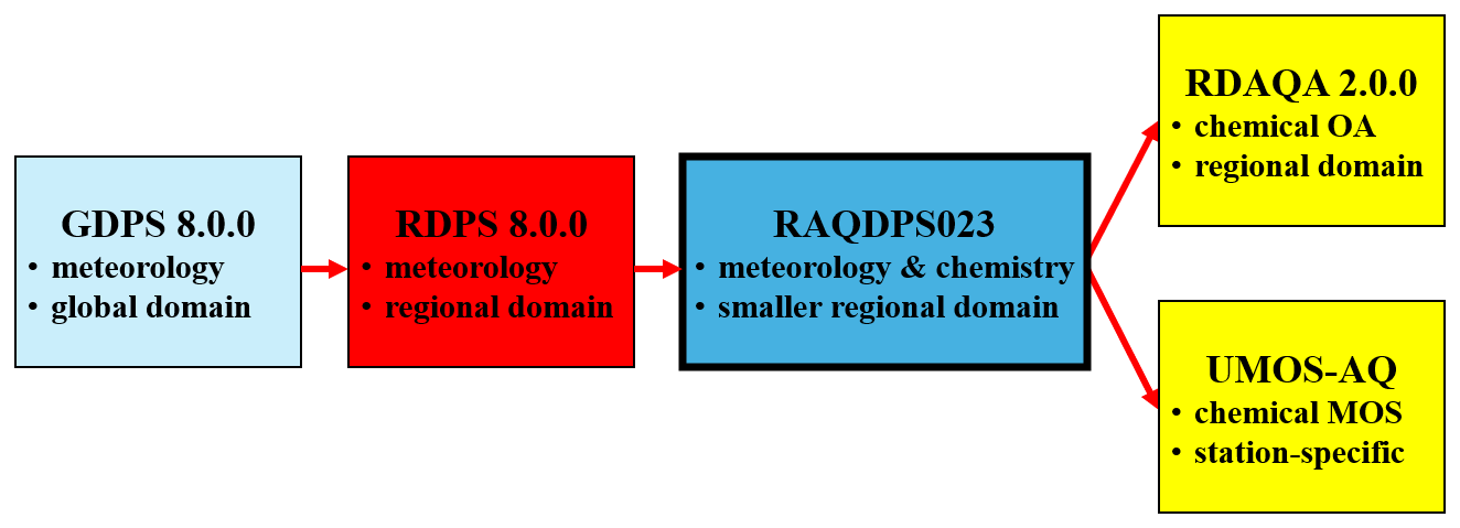
Figure 1RAQDPS023 “upstream” and “downstream” dependencies on other ECCC operational systems.
All three systems were based on GEM version 5.1.0. Most of the following description of GEM 5.1.0 thus applies to all three systems, but differences are noted where they occur. The main differences between the global and the two regional GEM-based systems were related to run configurations, namely domain size, horizontal grid spacing, integration time step, initialization, and boundary conditions.
2.1 Grids, coordinate systems, and nesting
The GDPS 8.0.0 employed an overset Yin–Yang global horizontal grid system that combines two perpendicular and overlapping, rotated latitude-longitude limited-area horizontal grids referred to as the Yin grid and the Yang grid. The globe is thus divided into two regions that look somewhat reminiscent of the covering and seams of a baseball (Qaddouri and Lee, 2011). This global grid system has two major benefits: it avoids pole-related singularities and convergence issues and it is suitable for use with massively parallel computers (Kageyama and Sato, 2004). Forecasts were made independently at each time step on the two regional LAM grids and were then reconciled across the overlap region (Qaddouri and Lee, 2011). The horizontal grid spacing for both the Yin and Yang grids used by the GDPS 8.0.0 was quasi-uniform 0.135° (∼ 15 km).
The rotated latitude-longitude LAM horizontal grid of the RDPS 8.0.0 covered the North American continent and adjacent oceans but was entirely a subdomain of the GDPS's Yin grid (Fig. 2). Horizontal grid spacing was quasi-uniform 0.09° (∼ 10 km). The RAQDPS023 horizontal grid, also shown in Fig. 2, was an embedded subgrid of the RDPS 8.0.0 grid with 0.09° grid spacing and grid-point superposition (i.e., co-location). The RDPS 8.0.0 horizontal grid was 1108 × 1082 in size vs. 772 × 642 for the RAQDPS023 horizontal grid. The smaller domain of the chemical weather model was necessary to balance the additional computational burden of the MACH chemistry module (see Sect. 4.1).
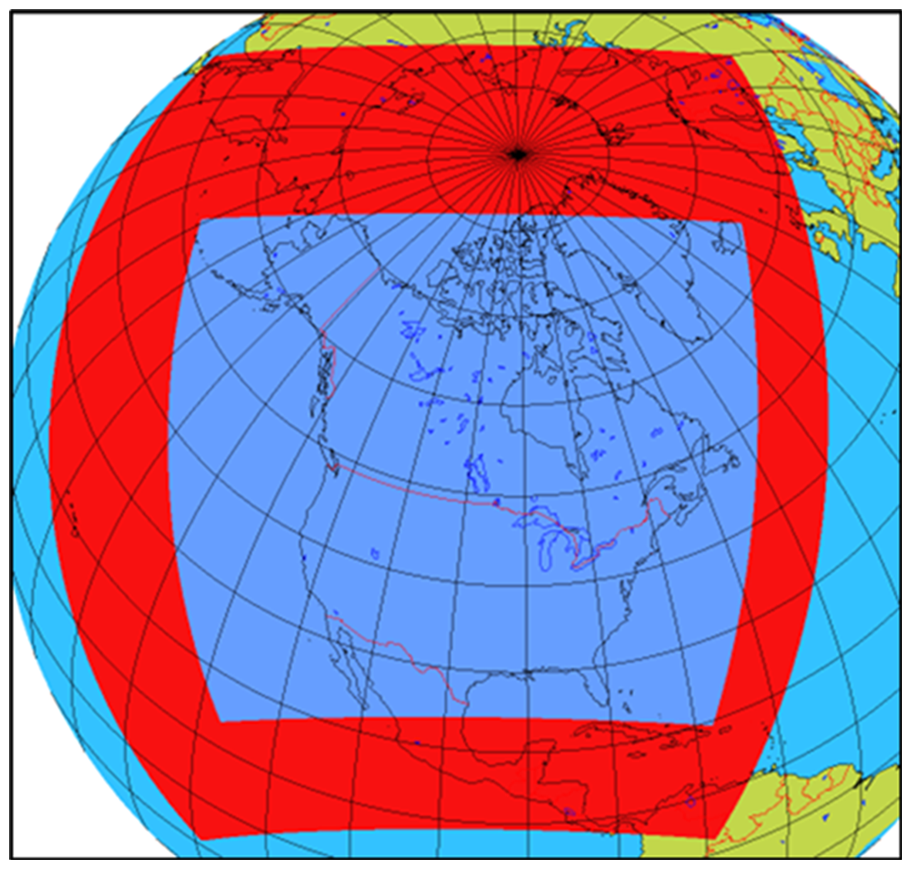
Figure 2Horizontal domains of RAQDPS023 (blue inner area) and RDPS 8.0.0 (surrounding red area plus blue inner area).
In terms of finite differencing, the horizontal discretization used for all three model grids was an Arakawa C grid, which Côté et al. (1998a) argued is more suitable for massively parallel computer architectures and for mesoscale applications. The vertical discretization for all three model grids was a staggered Charney–Phillips grid that was used with a log-hydrostatic-pressure-type ζ (or hybrid) vertical coordinate (Holdaway et al., 2013a, b; Girard et al., 2014). The GDPS 8.0.0, RDPS 8.0.0, and RAQDPS023 also all used the same 84 hybrid vertical levels stretching from the Earth's surface to 0.1 hPa. The lowest momentum “full” hybrid levels were located at approximately 20, 61, 114, 181, and 263 m a.g.l., and the lowest thermodynamic “half” hybrid levels were located at approximately 10, 40, 87, 147, and 222 m a.g.l. Vertical layer thickness was monotonic increasing with distance from the Earth's surface to the upper troposphere (where it then decreased to better resolve the tropopause region), and there were 11 thermodynamic hybrid levels located within the first kilometer above the surface.
GDPS 8.0.0 forecasts started before RDPS 8.0.0 forecasts so that one-way nesting could be used to supply meteorological lateral boundary conditions (LBCs) from the global weather forecasts to the LAM regional weather forecasts (Benoit et al., 1997; Ritchie et al., 2022; see also Sect. 4.2). Similarly, RDPS 8.0.0 forecasts started before RAQDPS023 forecasts so that one-way nesting could again be used to supply meteorological LBCs from the RDPS 8.0.0 LAM forecasts to the RAQDPS023 LAM forecasts (see Figs. 1 and 2 and Sect. 4.2). This one-way nesting technique is sometimes referred to as “piloting”. In fact, successive versions of the RAQDPS have been “piloted” or “driven” by successive versions of the RDPS since 2009 (Table A1).
2.2 RAQDPS023 meteorological configuration
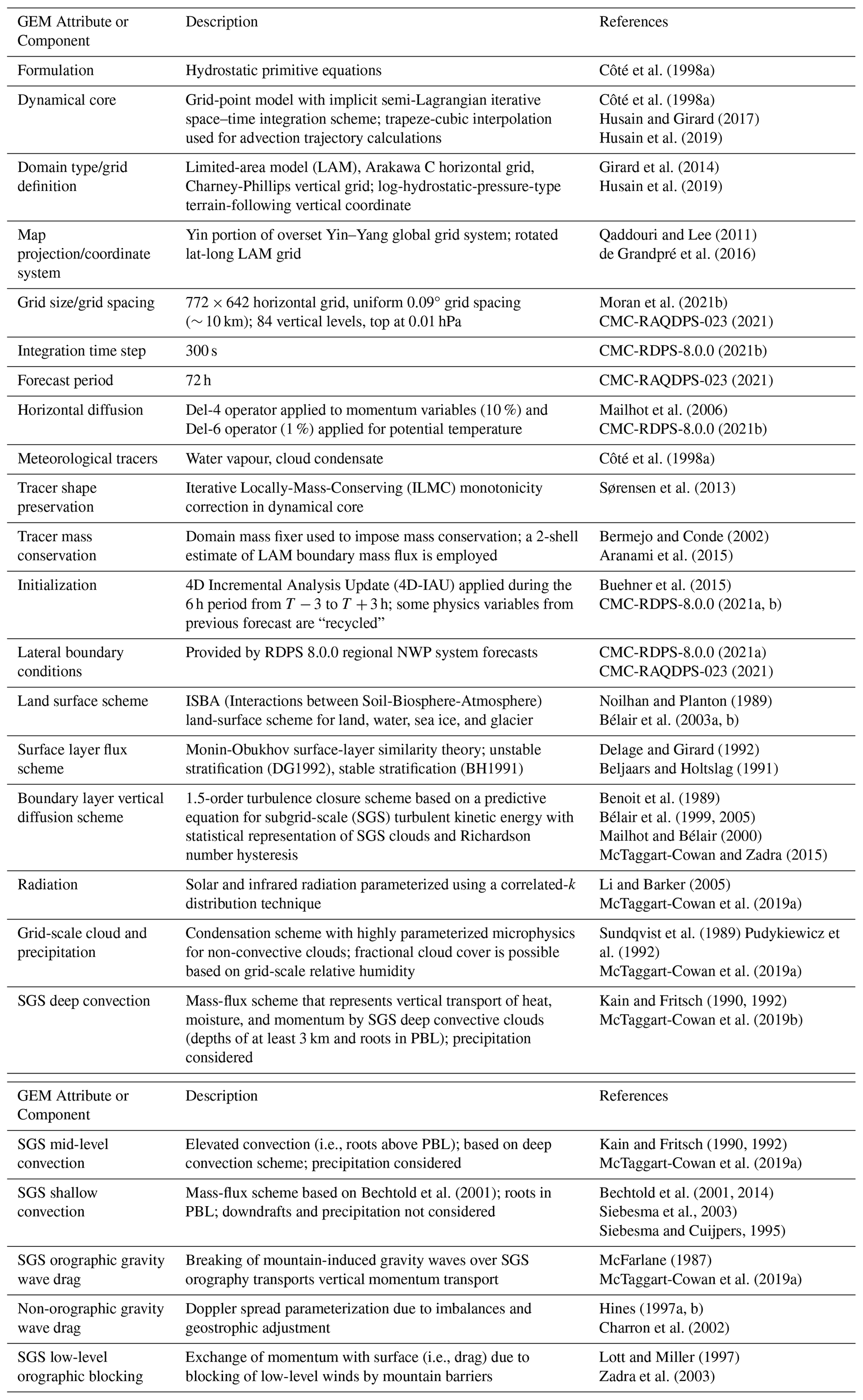
Table 1 provides a concise summary of the meteorological components and attributes of the RAQDPS023, including the dynamical core and various physical parameterizations. References are also provided for each component. These components and attributes were identical to those used by the RDPS 8.0.0 with two exceptions: horizontal domain size and LBC source (cf. CMC-RDPS-8.0.0, 2021b). For further information about Table 1, McTaggart-Cowan et al. (2019a) provide an excellent recent summary of ECCC implementations of the physical parameterizations listed in Table 1, Sect. S1 also provides some information about many of these components and attributes, and Sect. 4 covers some computational aspects.
Table 1RAQDPS023 meteorological configuration and references for GEM host model (see also CMC-RAQDPS-023, 2021).
The MACH (Modelling Air quality and CHemistry) module is an online chemistry module embedded in the GEM NWP model code to produce the GEM-MACH chemical weather model. It predicts the evolution in time of concentrations and removal rates of a number of gas-phase chemical species, including O3 and NO2, as well as size- and composition-resolved PM. Many of the chemistry parameterizations used by the MACH module were adapted from two earlier ECCC atmospheric chemistry codes, the Canadian Aerosol Module (CAM), which was designed to represent aerosol processes in climate models (e.g., Gong et al., 1997a, b, 2002, 2003), and A Unified Regional Air Quality Modelling System (AURAMS) CTM, which was an offline AQ model with a size- and composition-resolved representation of PM developed by ECCC for research and policy applications (e.g., Moran et al., 1998; Zhang et al., 2002a; Gong et al., 2006; Stroud et al., 2008; Makar et al., 2009; Levy et al., 2010). Furthermore, as noted below several chemistry parameterizations used by AURAMS were adapted from an earlier regional CTM used by ECCC, the Acid Deposition and Oxidant Model (ADOM: Venkatram et al., 1988, 1992; Misra et al., 1989; Fung et al., 1991, Karamchandani and Venkatram, 1992; Macdonald et al., 1993; Li et al., 1994).
3.1 Alignment with weather forecast models
For the RAQDPS023 the GEM-MACH code version was updated from version 3.0.2 to version 3.1.0.0 (see Table A1 and Moran et al., 2021b). This updated version incorporates the GEM v5.1.0 code that was also used by the GDPS 8.0.0 and RDPS 8.0.0 (CMC-GDPS-8.0.0, 2021a; CMC-RDPS-8.0.0, 2021a).
As noted in Sect. 2.1 the RAQDPS023 meteorological configuration was also very closely aligned with that of the RDPS 8.0.0 regional weather forecast model. First, the RAQDPS023 employed (i) the same set of dynamics options and physics parameterizations as the RDPS 8.0.0, including those for advection, vertical turbulent diffusion, radiation, grid-scale and subgrid-scale (SGS) clouds and precipitation, and gravity wave drag and orographic blocking (Table 1), (ii) the same vertical grid and a closely related horizontal grid (the RDPS horizontal grid domain is larger; see Sect. 2.1 and Fig. 2), and (iii) the same dynamics/physics integration time step (Table 1). As a consequence, weather forecasts made by the two systems are nearly identical over the RAQDPS horizontal domain.
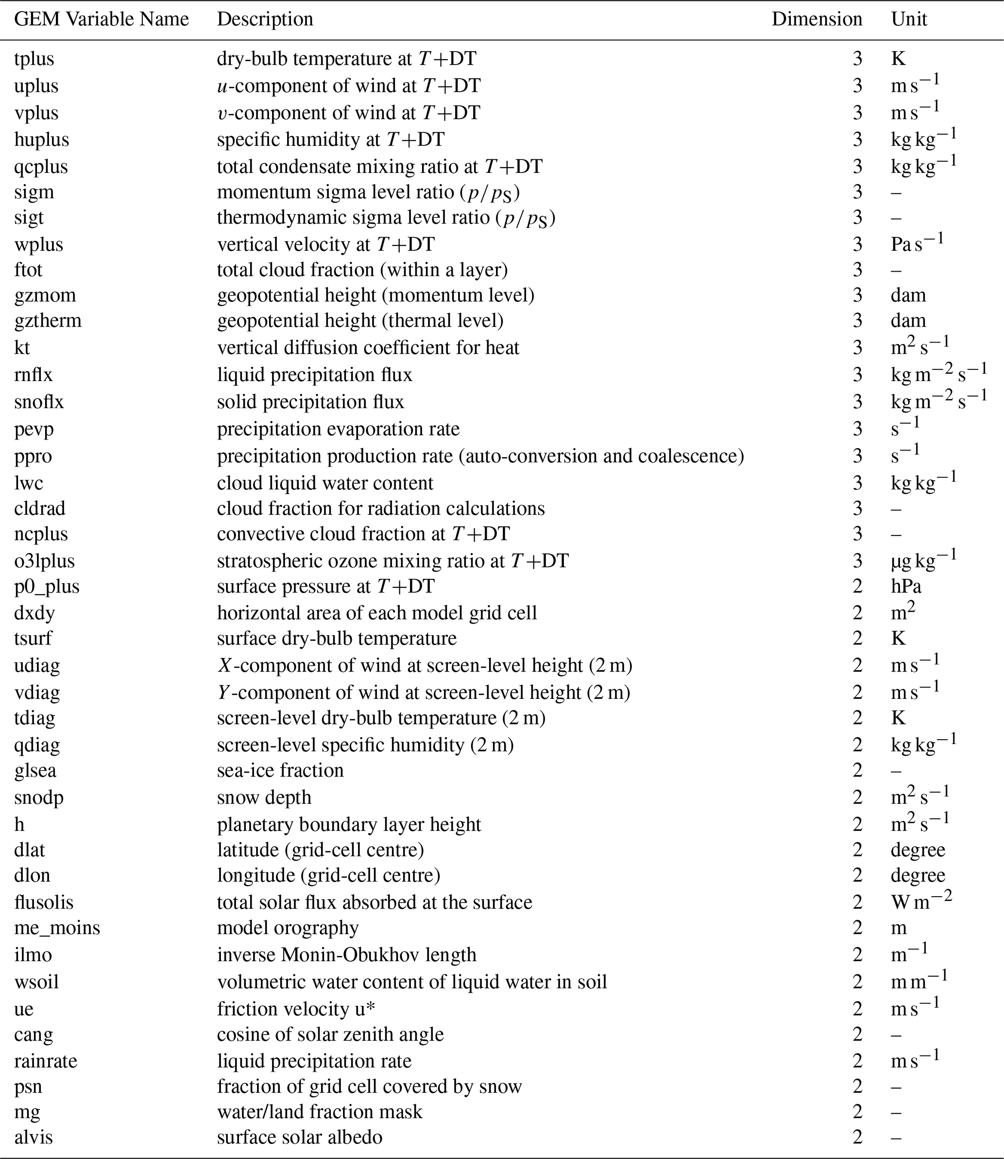
Second, the chemistry parameterizations used by the RAQDPS023 made use of many meteorological fields predicted by GEM. For example, the treatment of non-chemical cloud processes resides in the GEM physics module, which provides a number of meteorological fields to the MACH chemistry module, including cloud water mixing ratio (liquid and solid), precipitation production rate (auto-conversion and coalescence), precipitation evaporation rate, and precipitation vertical fluxes (both liquid and solid) (Mailhot et al., 1998; Gong et al., 2006, 2015; McTaggart-Cowan et al., 2019a). Table 2 summarizes the meteorological fields predicted by GEM that are needed by various MACH parameterizations in the RAQDPS023.
Table 2List of GEM-predicted meteorological fields needed by the MACH module. Two-dimensional fields are associated with the Earth's surface while three-dimensional fields are associated with the atmospheric column.
Third, as noted in Table 1 the GEM dynamical core used by the RAQDPS023 included two meteorological tracers: water vapour and cloud condensate. MACH considers a much larger number of chemical tracers, but these additional tracers are implemented in the GEM-MACH code in the same way as the meteorological tracers. In fact, MACH chemistry is essentially a run-time option of GEM that can either be activated to run GEM-MACH for chemical weather forecasts or not activated so that just GEM is run to make meteorological forecasts. Moreover, because GEM-MACH is an online system, it makes use of GEM schemes and Fortran2003 computer code for those dynamical and physical processes that are common to both meteorological and chemical tracers, including advection and vertical diffusion. One exception, however, is SGS convection, where SGS vertical transport of chemical tracers mirroring that of meteorological tracers has not yet been implemented.
Fourth, the same a posteriori treatments for shape preservation and mass conservation applied in the RDPS 8.0.0 for the advection of meteorological tracers (Table 1) are also applied in the RAQDPS023 for the advection of both meteorological and chemical tracers. Shape preservation and mass conservation are very relevant for a regional AQ model since there can be many sharp chemical concentration gradients in the vicinity of strong local emissions sources, and the resulting loss of shape preservation after advection can introduce negative concentrations (e.g., Flemming et al., 2015).
And fifth, in order to use the treatment of vertical turbulent diffusion from GEM for chemical tracers, area emissions and dry deposition of gases and particles are treated as flux boundary conditions at the bottom boundary. Note that two small differences in the parameterization of vertical diffusion for meteorological tracers vs. chemical tracers used by the RAQDPS023 were introduced in 2019 when the RAQDPS021 became operational (Moran and Ménard, 2019). In the RAQDPS021 the height of the lowest model half-level (i.e., first thermodynamic level) was reduced from 20 to 10 m and the scheme used to diagnose PBL height was also changed to a Rib-based scheme (Sect. S1.4), which resulted in PBL heights as small as 2 m being predicted under some stable conditions (Moran and Ménard, 2019). To avoid the occurrence of unrealistically high surface concentrations, two ad hoc modifications were introduced. One modification was to impose a minimum PBL height value of 100 m (other groups have imposed similar minimum values: e.g., Li and Rappenglueck, 2018). The second modification was to inject surface emissions equally into the two lowest model layers rather than just in the lowest layer as before 2019, which was equivalent to maintaining the 40 m lowest full-layer thickness considered before the RAQDPS021. Both modifications were carried over to the RAQDPS023.
3.2 Representation of particulate matter
The term “particulate matter” (or aerosol particles) refers to the mixture of solid particles and liquid droplets found suspended in air. The size of these particles can range from the “ultrafine” (aerodynamic diameters less than 0.1 µm) to the “giant” (aerodynamic diameters greater than 10 µm) (e.g., Wang et al., 2014a). PM is of interest for many reasons: for example, aerosol particles can interact with radiation via scattering and absorption (aerosol direct effect); they can act as condensation and ice nuclei in clouds and interact with cloud microphysics (aerosol indirect effect); and they can enter the human body via respiration, where they may impact human health. In fact, so-called “fine” particles (PM2.5) are a major cause of human mortality and morbidity (e.g., Lelieveld and Pöschl, 2017; Murray et al., 2020). As a consequence, many countries have legislated ambient air quality standards for PM2.5, including Canada (https://ccme.ca/en/air-quality-report, last access: 18 March 2026) and the U.S. (https://www.epa.gov/criteria-air-pollutants/naaqs-table, last access: 18 March 2026), and the World Health Organization has issued health-based guidelines for PM2.5 and PM10 ambient concentrations (WHO, 2021).
PM is a complex pollutant: (i) it is typically composed of particles with a wide size range spanning orders of magnitude; (ii) it can contain many different elements and compounds, both inorganic and organic; (iii) it is subject to many different physical and chemical processes (see below); and (iv) it has many different types of sources, including both particle-phase primary sources and gas-phase secondary sources (e.g., Fuzzi et al., 2015). Representing size- and composition-resolved PM in an AQ model with an affordable number of tracer species is thus a significant challenge both scientifically and computationally.
Two conceptual approaches have been used in AQ models to represent the PM size distribution: a sectional representation, in which the PM size distribution is divided in n contiguous, nonoverlapping, discrete size sections or size bins (e.g., Gelbard and Seinfeld, 1980; Seigneur et al., 1986; Jacobson, 1997; Zhang et al., 1999); and a modal representation, in which the PM size distribution is assumed to be composed of n distinct populations of particles, each of whose size distribution can be described by an analytical modal distribution function (e.g., Binkowski and Shankar, 1995; Whitby and McMurry, 1997). Many AQ models with a size-resolved treatment of PM have employed a sectional representation, (e.g., Jacobson, 1997; Kukkonen et al., 2012; Zhang et al., 2012a, b; WMO, 2020). For each model, though, the number of sections (n) that are considered must be chosen.
For GEM-MACH two different values of n have been used, depending upon the application. For operational AQ forecasting with the RAQDPS, only two size bins have been used in order to reduce model execution times: PM2.5 or “fine PM”, which corresponds to particle diameters in the 0–2.5 µm range; and PMcf or “coarse fraction”, which corresponds to particle diameters in the 2.5–10 µm range. Taken together these two size bins constitute PM10 (“coarse PM”). These two size bins were chosen to enable prediction of PM2.5 and PM10, the two PM size ranges of concern for AQ standards in North America, following the approach of an earlier size-resolved PM model (Middleton, 1997). These two size bins are also consistent with measurement studies, which have found that atmospheric aerosol volume and mass size distributions generally have only two distinct modes, an accumulation mode (0.1 to 2 µm diameter range) and a coarse mode (diameter > 2 µm), except for very clean conditions or close to sources of hot gases where a distinct (and smaller) nucleation or Aitken mode is evident (e.g., Whitby, 1978; Morawska et al., 1999). Whitby (1978) also argued that there is little interaction between particles in the accumulation and coarse modes. Note too that PM2.5 and PM10 are the two PM size ranges that are considered by the Canadian, U.S., and Mexican national emissions inventories (see Sect. 3.11.1) and by a number of North American surface measurement networks (e.g., Brook et al., 1999b; NSTC, 2013; Moran et al., 2026). However, as discussed below in Sect. 3.3.4 and 3.8 it was necessary to introduce an additional subdivision of the PM2.5 and PMcf size bins in order to reduce errors in the numerical solution of several aerosol process parameterizations. It is should be noted that some model applications do need the PM size distribution to be resolved in more detail, such as calculations of atmospheric visibility and aerosol optical depth or studies of meteorology-aerosol interactions through aerosol direct and indirect effects. For such applications GEM-MACH is typically run with 12 size bins (e.g., Gong et al., 2015; Makar et al., 2015a, b; Ghahreman et al., 2021; Majdzadeh et al., 2022).
Another complication related to the PM size distribution is that there are multiple definitions of aerosol particle diameter. The most common definition is aerodynamic diameter, which is defined as the diameter of a spherical particle with a density of 1 g cm−3 that behaves similarly to the particle of interest. This is the definition used for PM2.5 and PM10 for AQ standards, for reporting most ambient measurements, and for preparing emissions inventories. However, CTMs like GEM-MACH consider Stokes diameter, which is the diameter of a spherical particle that behaves similarly to the particle of interest and has the same density. Stokes diameter is equal to the aerodynamic diameter divided by the square root of the particle density (e.g., Seigneur and Moran, 2004), and this difference should be considered when comparing model-predicted PM values with observed PM values (see companion paper by Moran et al., 2026).
While it is important for the RAQDPS to predict PM2.5 “bulk” mass or total mass since PM2.5 total mass is one of the three species considered by the AQHI, it is also important for the RAQDPS to resolve the chemical composition of PM2.5 and PM10 since many PM properties and processes depend on a particle's chemical composition. In order to achieve this representation with only a modest number of chemical components so as to reduce computational costs, just nine components were considered by the RAQDPS023: sulfate (SU); nitrate (NI); ammonium (AM); elemental carbon (EC); primary organic matter (POM); secondary organic matter (SOM); crustal material (CM); sea salt (SS); and aerosol water (WA). This set of chemical components is consistent with the approach of three North American PM2.5 speciation measurement networks (CSN, IMPROVE, NAPS) to report PM2.5 chemical composition (see Dabek-Zlotorzynska et al., 2011; Chow et al., 2015) and with other AQ models that resolve PM composition (e.g., Table 6 of Kukkonen et al., 2012). Note, however, that all of these chemical components must be considered to be “lumped” species. In the case of particle SU, NI, and AM, they do not account for the molecular or stoichiometric form of these three inorganic constituents, which controls particle acidity. For example, particle SU may be present as sulfuric acid (H2SO4(aq)), ammonium sulfate ((NH4)2SO4(s)), ammonium bisulfate ((NH4HSO4(s)), or letovicite ((NH4)2H(SO4)2(s)) (e.g., Saxena et al., 1983; Makar et al., 2003b). Particle EC, which is often referred to as black carbon (BC), is implicitly defined by the source-testing and ambient measurement methods used to measure it (e.g., Chow, 1995; Chow et al., 2015, 2018). Particle organic matter (POM and SOM) is composed of other elements such as hydrogen, oxygen, sulfur, and nitrogen, in addition to carbon (e.g., Turpin and Lim, 2001; Pang et al., 2006; Malm and Hand, 2007; Philip et al., 2014). Particle CM (or soil dust) is composed of oxides of silicon, various metals (e.g., iron, aluminum, titanium), base cations (sodium, calcium, magnesium, and potassium), and carbonate (e.g., Malm et al., 2004; Dabek-Zlotorzynska et al., 2011; Hand et al., 2017). And particle SS is a complex mixture of multiple salts and organics in addition to NaCl (e.g., White, 2008; Ault et al., 2013).
One additional aspect of PM composition is its mixing state, which refers to the variation of PM chemical composition with particle size (e.g., Heintzenberg, 1989; Jacobson, 2001; Zhu et al., 2015). At one extreme, referred to as an internal mixture, all aerosol particles of a given size at a given point in space and time are assumed to have the same chemical composition. At the other extreme, referred to as an external mixture, each aerosol particle of the same size may be composed of any one of many pure chemical species. And between these two extremes lies a very wide range of transitional mixing states. Mixing state affects a particle's hygroscopicity, organic absorptivity, and radiative properties (Stevens et al., 2022). MACH assumes that each PM size bin is internally mixed (Gong et al., 2003; Park et al., 2011; Stevens et al., 2022). This assumption has the advantage of minimizing the number of PM chemical components that must be considered since no special considerations must be made for mixing state. It is least good close to emission sources of primary PM but becomes more realistic as aerosol particles age and undergo condensation and coagulation processes (e.g., Winkler, 1973).
Size- and composition-resolved atmospheric PM was thus represented in the RAQDPS023 with two internally-mixed size bins and nine chemical components for a total of 18 size bin-chemical component tracers (e.g., PM2.5-EC, PMcf-NI). Sixteen of these PM tracers were prognostic fields and were advected while the two size bin-aerosol water tracers were diagnostic fields that were estimated by the Hänel (1976) scheme or the HETV code (Sect. 3.3.5 and 3.6). Although each size bin was assumed to be internally mixed, the chemical composition of the two size bins could be different. Mass mixing ratio (MMR) with units of µg size bin-component per kg dry air was used in the PM conservation-of-mass equations in MACH to describe aerosol particle abundances. Mixing ratios have the advantage of being independent of pressure and temperature. While molar (or volume) mixing ratio is an official SI unit for species abundance in air (Schwartz and Warneck, 1995), MMR is a more appropriate choice when the chemical composition of a constituent is not known or is not well-defined as is the case for “lumped” chemical species such as the above nine PM chemical components. MMR units were also used for gaseous species in the RAQDPS023 for consistency, although unit conversions may be performed before and after some process operators (e.g., gas-phase chemistry).
3.3 Aerosol microphysical schemes
A number of physico-chemical processes affect the PM population and its size distribution and chemical composition: (i) emission of primary particles of different sizes and composition; (ii) nucleation of new ultrafine particles from gas-phase precursors; (iii) growth of existing particles via condensation of non-water vapours and the shrinkage of particles via volatilization of particulate species to the gas phase (i.e., gas-particle partitioning); (iv) collision and coagulation of particles; (v) swelling and activation of particles due to water-vapour sorption processes; and (vi) size-dependent removal of particles via dry and wet deposition processes. CTMs that resolve the PM size distribution should in principle simulate all of these processes. However, urban-scale CTMs often neglect nucleation (by assuming that condensation prevails under conditions with moderate to high PM concentrations) and coagulation (which is typically slow compared to other processes), but regional-scale CTMs with their larger domains and longer transport times may consider these two processes. As described in this section and in Sect. 3.10 and 3.11.1, MACH represents all of the above physical processes as well as several aerosol chemical processes that are described in Sect. 3.5 to 3.7.
3.3.1 Nucleation scheme
Nucleation refers to the creation of new particles by the formation of molecular clusters by low-volatility gases such as sulfuric acid vapour H2SO4(g) and some organic species. Such nucleation-mode particles are tiny, with diameters less than 3 nm (Semeniuk and Dastoor, 2018). MACH uses a parameterization of the nucleation process based on classical nucleation theory for sulfuric acid and water binary homogeneous nucleation as proposed by Kulmala et al. (1998) and adopted in CAM (Gong et al., 2003). The expression for particle nucleation rate is dependent on sulfuric acid vapour abundance, temperature, and relative humidity (RH), and the particle mass that is created is assigned to the smallest PM size bin, which for the RAQDPS023 is the PM2.5 size bin.
3.3.2 Condensation/evaporation scheme
Aerosol particles will grow in size due to the condensation of gas-phase species onto these particles but will shrink in size due to the evaporation of semi-volatile gases from these particles. A modified Fuchs-Sutugin equation is used to calculate the condensation rate for H2SO4(g) onto aerosol particles (Fuchs and Sutugin, 1971; Hegg, 1990; see Eq. (A14) of Gong et al., 2003). The expression for the condensation rate to a single particle is linearly dependent on particle diameter and H2SO4(g) ambient vapour pressure, where the surface vapour pressure of H2SO4 at the particle surface is very small and is assumed to be zero so that H2SO4 mass transfer is one-way from the gas phase to the particle phase (Russell et al., 1994). The overall condensation rate to a given particle size bin also depends on the particle number concentration for that bin (Np,i). This quantity is calculated as the total dry volume of the eight PM chemical components in that bin (i.e., excluding aerosol water) divided by the volume of a spherical particle whose diameter is the arithmetic mean of the size boundaries of that bin. Note that condensation to multiple size bins will occur simultaneously. The condensation process does not change the total particle number density, but it does increase the mass of individual particles. As a consequence, some particles in size bin i may grow in size enough to move to a larger size bin. The treatment of such particles by size “rebinning” is described in Sect. 3.8.
One additional complication is that nucleation and condensation processes compete for H2SO4(g). Following the procedure used in CAM (Gong et al., 2003), the division of H2SO4(g) between these two processes for each time step is calculated by solving the time rate of change equation of H2SO4(g) accounting for both production of H2SO4(g) and removal by nucleation and condensation. As noted by Morawska et al. (1999), however, most of the time removal by condensation will dominate removal by nucleation.
The condensation of those organic gases that partition to the particle phase to form SOM (Sect. 3.7) is treated very similarly to the condensation of H2SO4(g). The relative condensation rate of H2SO4(g) to each PM size bin is used as a proxy for the relative condensation rates of these organic gases to each PM size bin.
3.3.3 Coagulation scheme
Coagulation is the process by which two or more aerosol particles can combine through collision. Coagulation acts to reduce the number concentration of aerosol particles, especially small particles, and hence serves as a control on the evolution of the number concentration of nucleation-mode and directly-emitted accumulation-mode particles. Four distinct physical processes may result in coagulation of particles: Brownian motion; gravitational collection; turbulent inertial motion; and turbulent shear (e.g., Jacobson, 1999; Seinfeld and Pandis, 2016).
MACH follows CAM by using a semi-implicit numerical solution of the general coagulation equation (Jacobson et al., 1994) to compute the coagulation rate and intersectional transfer of aerosol particles (Gong et al., 2003). This scheme conserves bulk particle volume for any time step but results in the transfer of particle volume from smaller to larger size bins. Since MACH assumes that each PM size bin is internally mixed, the mass concentration change of each chemical component can be computed from the calculated volume change of any size bin due to coagulation. Note that the coagulation coefficient is dependent on the “wet”, or real, size of aerosol particles, not the dry size (see Sect. 3.3.5).
3.3.4 Gravitational settling and dry deposition schemes
Particles in the atmosphere undergo gravitational settling (or sedimentation) towards the Earth's surface under the influence of gravity. The downward vertical speed is called the terminal settling velocity and depends on a particle's density and the square of its wet diameter (e.g., Seinfeld and Pandis, 2016). Particles close to the Earth's surface can then be removed from the atmosphere by dry deposition, a complicated process that depends on near-surface meteorological conditions, the nature of the underlying surface, and particle density and size (e.g., Slinn, 1977; Ruijgrok et al., 1995).
Size-resolved particle dry deposition in MACH is represented using a scheme proposed by Zhang et al. (2001), which accounts for a number of relevant processes: turbulent transfer; Brownian diffusion; impaction; interception; gravitational settling; and particle rebound. Calculated particle dry deposition velocities have a strong dependence on particle size with a minimum value at particle diameters of about 1 µm and larger values for both smaller and larger particle sizes (Gong et al., 2003). Surface characteristics for 15 different land-use categories are considered for this calculation (e.g., Zhang et al., 2001; Table S7 of Makar et al., 2018b). Particle dry deposition is only applied at the lowest model level, where the sum of dry deposition velocity and terminal settling velocity is used, whereas gravitational settling occurs throughout the vertical column.
A revised numerical solution for the gravitational settling process was introduced in the RAQDPS023 based on a semi-Lagrangian advection approach. Vertical back trajectories were calculated from the settling and deposition velocities for each particle size, and then mass-conservative interpolation was used to determine the new vertical concentration profile and deposition flux to the surface (Makar et al., 2018a). This new scheme replaced a previous numerical scheme based on an analytical exponential decay rate and better accounts for the model's decreasing vertical grid spacing close to the Earth's surface (Sect. 2.2). The result was a reduction of the rate of removal by downward particle advection. As a consequence, near-surface PM concentrations increased by as much as 0.5 µg m−3 compared to those predicted using the old solution scheme (Moran et al., 2021b).
Lastly, to address the strong dependence of particle dry deposition and sedimentation on particle size (e.g., Zhang et al., 2001; Gong et al., 2003), the numerical solution of these processes was modified for the simplified two-bin description of the PM size distribution early in the development of the RAQDPS to reduce numerical errors. The two PM size bins were each subdivided into six sub-bins. Settling velocities were then estimated for each sub-bin based on a third-order polynomial fit to a typical log10(settling velocity) as a function of log10(radius) that was determined using a stand-alone version of the code. Dry deposition velocities were also calculated for each sub-bin based on a weighted average of third-order polynomial fits to a typical log10(dry deposition velocity) as a function of log10(radius) for non-urban land surfaces and urban land surfaces (which has higher values). Revised values of settling velocity and dry deposition velocity for the two size bins were then calculated as logarithms of the sum of the exponentials of the sub-bin values. The revised values of the settling velocities for PM2.5 and PMcf based on the sub-bin division were roughly 30 % smaller and 100 % larger, respectively. The revised values of the dry deposition velocities for PM2.5 and PMcf, on the other hand, were roughly 100 % larger and 50 % smaller. Analogous modifications to the numerical solution of three other aerosol processes (condensational growth, aqueous-phase chemistry, and inorganic heteorogeneous chemistry) to address intersectional mass transfer in the simplified two-bin configuration are described in Sect. 3.8.
3.3.5 Hygroscopic growth and aerosol activation schemes
The hygroscopic growth of mixed aerosol particles at subsaturation conditions (i.e., RH < 1), which is sometimes referred to as swelling, can result in substantial aerosol water component (WA) values. For example, Tsyro (2005) has suggested that for T=20 °C and RH = 50 % aerosol water may contribute 20 %–35 % of annual mean PM2.5 concentrations in Europe. Nguyen et al. (2016) have shown based on field study measurements from around the world that aerosol water is ubiquitous and at rural locations contributed on average 3 µg m−3 and 35 % of PM1 total mass. In fact, at high RH values the aerosol water component can dominate aerosol particle composition and mass (e.g., Tang and Munkelwitz, 1994; Nguyen et al., 2016; Widziewicz-Rzońca and Tytła, 2020).
The RAQDPS23 calculates aerosol water using a mixing rule for soluble components (SU, NI, AM, POM, SOM, SS), whereas EC and CM are assumed to be hydrophobic (Gong et al., 2003, Appendix A1). This approach follows that of Hänel (1976). Note that the aerosol water component WA is also diagnosed independently by the HETV scheme (Sect. 3.6).
Under supersaturated conditions (i.e., RH > 1) hygroscopic aerosol particles can grow rapidly by water-vapour condensation to form cloud droplets, whose diameters typically fall in the 10–200 µm range vs. 500–8000 µm for raindrops (e.g., Jacobson, 1999). This process is called aerosol activation but may also be referred to as nucleation scavenging or droplet nucleation, and aerosol particles that can be activated are referred to as cloud condensation nuclei (CCN). Aerosol particle activation is important because it may result in modification of the PM mass and size distributions within and below clouds by aqueous-phase chemistry and wet removal (Sect. 3.5 and 3.10). This trio of processes is referred to collectively as cloud processing. However, whether a CCN particle is activated depends on the level of supersaturation and the particle's size and physical and chemical properties (e.g., Gong et al., 2011).
Two different parameterizations of aerosol particle activation are available in MACH (Gong et al., 2015). For the RAQDPS023, MACH uses the empirical aerosol activation scheme of Jones et al. (1994) to determine the cloud droplet number concentration Nd in a cloud as a function of the particle number concentration Np. This scheme permits the calculation of a critical particle radius above which all aerosol particles are assumed to be activated (Gong et al., 2006). The portion of aerosol particles incorporated in these cloud droplets is then determined by adding particles from the largest size bins in descending order of size until Nd is reached (Gong et al., 2006, 2015). Next, the bulk cloud liquid water content from GEM (Table 2) is distributed evenly to all activated aerosol particles, after which the cloud droplet size associated with each PM size bin can be determined (Gong et al., 2006). Information about the activated aerosol particles, including their wet diameter, is then available for use by other aerosol process parameterizations, including aqueous-phase chemistry and in-cloud scavenging. Note that one consequence of this scheme is that only some of the particles in a size bin may be activated when the critical particle radius for activation falls between the lower and upper boundaries of a size bin. For the RAQDPS023 with only two size bins, all of the particles in the PMcf size bin (i.e., Np,2) must be activated before any particles in the fine size bin can be activated.
3.4 Gas-phase chemistry scheme
Numerous gas-phase chemical reactions occur in the atmosphere (e.g., Jenkin et al., 2015), and some important gas-phase species such as O3 and hydrogen peroxide (H2O2) are reaction products only and are not directly emitted to the atmosphere. It is thus necessary to represent these reactions in a CTM (e.g., Dodge, 2000), but it is also challenging. In particular, volatile organic compounds (VOCs) play a key role in determining the oxidative state of the atmosphere because they may react with three important oxidants: hydroxyl radical (OH); nitrate radical (NO3); and O3 (e.g., Atkinson, 1990; Seinfeld and Pandis, 2016). As a consequence VOCs influence photochemistry, PM formation, and acid deposition. However, thousands of VOC species with varying chemical and physical properties, including OH reactivity, vapour pressure, and solubility, are emitted to the atmosphere (e.g., Makar et al., 2003b), and it is not computationally feasible for three-dimensional AQ models to consider the chemical reactions of all of these individual species. Instead, a number of parameterized gas-phase chemistry mechanisms have been developed that consider reduced-form or condensed representations of the full atmospheric chemical system by “lumping” or aggregating groups of VOC species with similar chemical properties together in order to reduce the number of species and chemical reactions that must be considered (e.g., Carter, 1990; Middleton et al., 1990; Kuhn et al., 1998; Dodge, 2000).
The RAQDPS023 used a modified version of the ADOM-2 gas-phase chemistry mechanism to parameterize tropospheric chemistry (Stockwell and Lurmann, 1989; Pudykiewicz et al., 1997; Moran et al., 1998). The ADOM-2 mechanism, which itself was an update of the ADOM-1 condensed mechanism (Lurmann et al., 1986; Fung et al., 1991), was designed to give an accurate representation of hydrocarbon gas-phase reactivity using a modest number of model VOC species. It employs a “lumped molecule” approach (Dodge, 2000) to define 16 lumped VOC species and eight organic radicals in addition to CH4 and C2H6 plus 21 inorganic species. Table 3 lists these 46 ADOM-2 gas-phase chemical species and some of their properties, and Table 4 lists the ADOM-2 mechanism's 114 associated chemical reactions, including 16 photolytic reactions that depend on sunlight.
Table 3List of ADOM-2 gas-phase model chemical species and their physical and model properties. GMM stands for gram molar mass and DDF stands for dry deposition scaling factor (see Sect. 3.9).
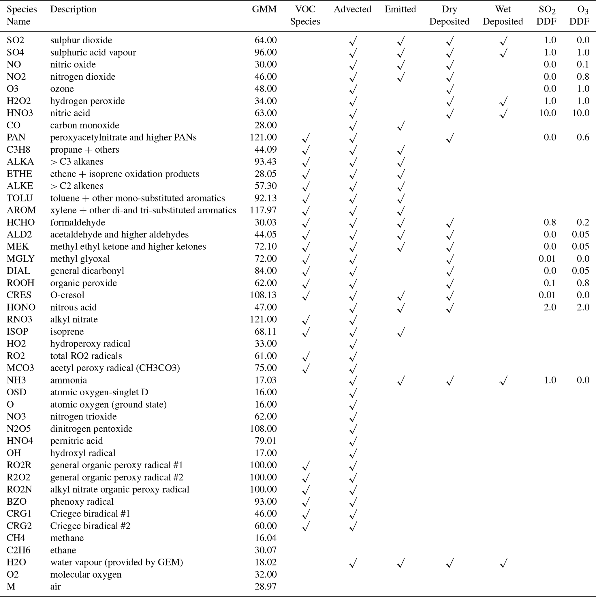
Note from Table 3 that the abundances of 42 of these model gas-phase species were forecast and advected while the abundances of four model species (CH4, C2H6, O2, M) had specified, time-invariant vertical profiles and were not advected or modified by gas-phase chemistry but were considered as reactants in some of the ADOM-2 reactions (Table 4), as was H2O, the water vapour field from GEM (huplus; see Table 2). Eighteen of the advected gas-phase species were organic species, of which 11 were emitted along with eight inorganic species (Table 3). Only two of the ADOM-2 VOC species that were emitted were individual or unlumped species, namely formaldehyde (HCHO) and isoprene (ISOP; C5H8). The other nine were lumped species, and this high degree of lumping imposes a limitation for evaluating model predictions of VOC species (e.g., Stroud et al., 2008; Moran et al., 2026).
Table 4List of ADOM-2 gas-phase mechanism chemical reactions and reaction rate coefficients in KPP-compliant input format (Damian et al., 2002; Sandu and Sander, 2006). Chemical reactions are listed in the left-hand column, and include first-, second-, and third-order reactions. All of the chemical species are defined in Table 3, except for hυ, which indicates a photon of light of frequency υ, and DUMMY, which indicates a non-reacting species. The reaction rate coefficients listed in the right-hand column have units of s−1, cm3 mol−1 s−1, and cm6 mol−2 s−1 for first-, second-, and third-order reactions, respectively. SUN is normalized sun intensity and ranges from 0 at night and 1 at noon (but is replaced during simulations by model-calculated J values); TEMP corresponds to ambient atmospheric dry-bulb temperature (K); the ARR2 function describes the reaction rate coefficient in Arrhenius form, where the first argument is the preexponential factor and the second argument provides the value; the TYPE5 function calculates third-order, pressure- and temperature-dependent reaction rate coefficients based on Troe theory (e.g., Seinfeld and Pandis, 2016), where the first argument specifies the F factor, the second and third arguments specify the high-pressure limiting rate coefficient, and the fourth and fifth arguments specify the low-pressure limiting rate coefficient; RCONST(n) is the reaction rate coefficient for the nth reaction; and CFACTOR is a units conversion factor.
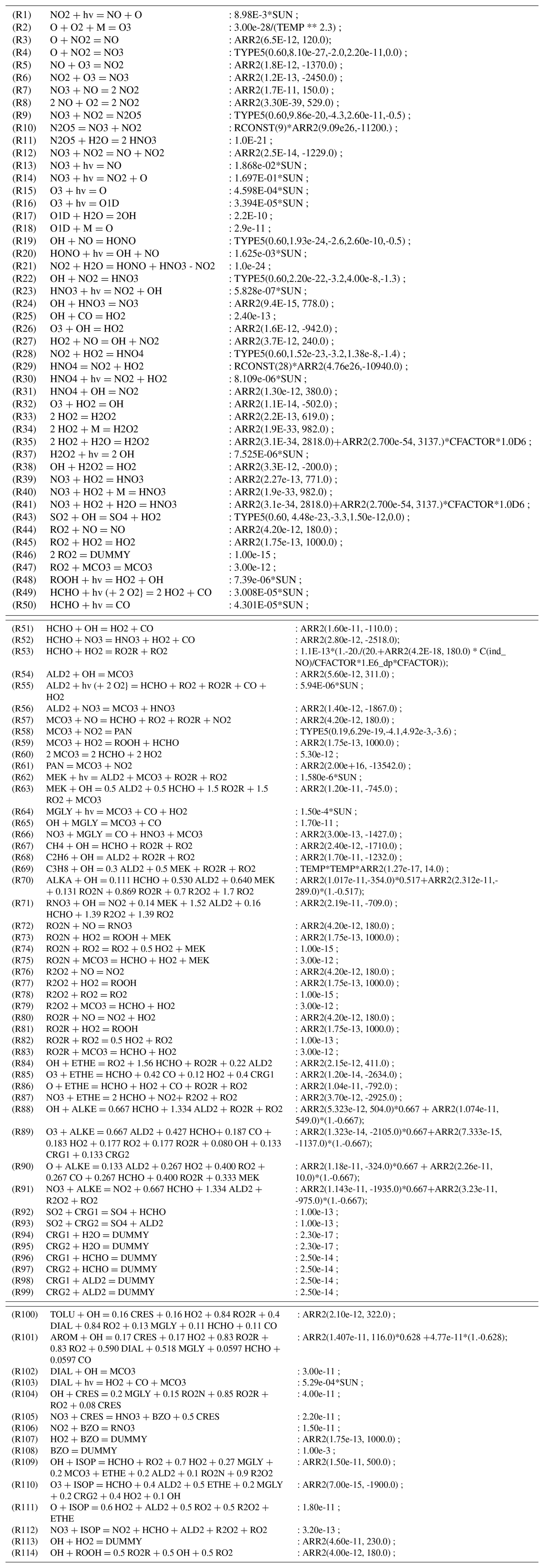
Note that Reaction (R21) represents a two-step heterogeneous reaction on a water surface and that Reactions (R36) and (R42) have been combined with Reactions (R35) and (R41), respectively.
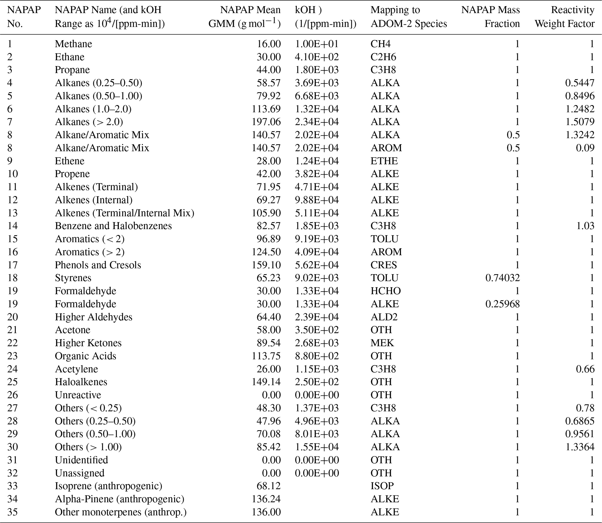
The calculation of lumped ADOM-2 VOC emissions begins with the assignment of individual emitted VOC species to one of the 32 VOC categories proposed by Middleton et al. (1990) to aggregate the 1980 National Acid Precipitation Assessment Program (NAPAP) anthropogenic VOC emissions inventory or to three additional biogenic categories (Isoprene, Alpha- and Beta-Pinene, and Other Monoterpenes) suggested by Makar et al. (2003b). These 35 VOC categories are then further lumped to the 11 emitted ADOM-2 VOC species using mole-based reactivity weights (see Table 5). Most of the ADOM-2 VOC species represent tens, hundreds, or even thousands of individual VOC species. For example, the ADOM-2 C3H8 lumped VOC species includes propane (C3H8) as would be expected, but it also includes benzene, acetylene, and some other lower-reactivity species (e.g., alcohols, ethers, and esters) that are assigned to NAPAP category 27 (e.g., Plummer et al., 2001; Makar et al., 2003b). The ETHE lumped VOC species includes ethene (C3H8), but it also includes isoprene oxidation products such as methacrolein and methyl vinyl ketone in order to implement a condensed isoprene chemistry mechanism used by the Carbon Bond-IV chemistry mechanism (Gery et al., 1988, 1989; Stockwell and Lurmann, 1989; Stroud et al., 2008). Note that emissions of acetone, organic acids, haloalkenes, and three other NAPAP VOC categories (26, 31, 32) are not included in emissions for the ADOM-2 mechanism due to their low or unknown reactivities (referred to collectively in Table 9 as EOTH). While the omission of these categories is defensible from a reactivity perspective, the neglect of organic acids in particular may remove a potential source of secondary organic aerosol (e.g., Makar et al., 2003b; Fisseha et al., 2004).
Table 5List of NAPAP VOC classes and properties and mapping to ADOM-2 lumped VOC species. The “Others” classes include alcohols, ethers, alcohol ethers, esters, etc., while OTH includes all low- and non-reactive species.
Rate constants for the inorganic reactions considered by the ADOM-2 mechanism were based largely on the recommendations of DeMore et al. (1987) while those for the organic reactions were based largely on Atkinson et al. (1992). The rates of the 16 photolytic reactions in Table 4 are expressed as the abundance of photoactive species multiplied by the photodisassociation rate coefficient (i.e., J value). The ADOM-2 photodisassociation rate coefficients were calculated from lookup tables of clear-sky actinic flux from Peterson (1976), which were based on the radiative transfer model of Dave (1972) and absorption cross-sections and photodisassociation quantum yields from DeMore et al. (1987) (Stockwell and Lurmann, 1989). The photodisassociation rate coefficients for and depend on both altitude and solar zenith angle whereas the other photodisassociation rate coefficients depend only on solar zenith angle and species-dependent scale factors (Kelly et al., 2012). Lastly, to account for the effect of clouds on clear-sky photolysis rate constants, the total cloud fraction field fcld (ftot in Table 2), which accounts for both resolved and SGS clouds in a model layer, and cloud liquid water content field (lwc in Table 2) predicted by GEM were used to scale the precalculated clear-sky J values following an algorithm from Chang et al. (1987). More details are given in Majdzadeh et al. (2022). Note that the performance of the ADOM-2 gas-phase mechanism was compared to a number of other gas-phase chemistry mechanisms by Kuhn et al. (1998), and its predictions were found to be close to the median for the nine mechanisms tested.
To integrate the chemistry tracer conservation-of-mass equations in time, the Young and Boris (1977) predictor-corrector method was used to solve the gas-phase chemistry step of the process operator splitting sequence (see Sect. 4.1). This asymptotic algorithm, which typically must use much smaller integration time steps than the overall MACH chemistry time step of 900 s due to the stiffness of the ADOM-2 chemical system, is integrated over the MACH chemistry time step.
The treatment of stratospheric chemistry in the RAQDPS023 was much simpler than that for tropospheric chemistry. The LINOZ scheme for ozone stratospheric chemistry (McLinden et al., 2000) was used to forecast ozone concentrations while concentrations of other species were only affected by dynamics and physics. The definition of the stratosphere used to apply the LINOZ scheme in each grid column was either those vertical levels located above 100 hPa or with specific humidity less than 10 ppmv. The ADOM-2 scheme was used below these levels. The LINOZ scheme was also implemented in the GDPS 8.0.0 to support the data assimilation of satellite-based ozone measurements (CMC-GDPS-8.0.0, 2021a).
3.5 Aqueous-phase chemistry scheme
Cloud chemistry, that is, aqueous-phase chemistry in cloud water, is an important pathway for the conversion of SO2 to SO (e.g., Barth et al., 2000; Gong et al., 2011). As well as referring to chemical reactions amongst various species in dilute aqueous solution in the cloud droplets, the term aqueous-phase chemistry usually encompasses two related processes: mass transfer of species between the gas phase and aqueous phase (absorption/condensation) inside clouds and the dissociation/ionisation in cloud water of certain dissolved species. Note that consideration of these processes is necessarily restricted to activated aerosol particles (Sect. 3.3.5).
MACH employs a slightly adapted version of the ADOM aqueous-phase chemistry mechanism, which considers 12 gas-phase and 13 aqueous-phase species together with 25 reactions, to represent these processes (Young and Lurmann, 1984; Fung et al., 1991). Note from Table 4 that one ADOM-2 mechanism species, NH3, does not participate in any gas-phase reactions, but NH3 gas participates in aqueous-phase and inorganic heterogeneous reactions (see also Sect. 3.6). Table 6 lists the 25 gas and aqueous species and Table 7 lists the 25 reactions that are considered by this condensed mechanism. Reactions (R19)–(R22) describe the four pathways for SO2 oxidation (i.e., S(IV) → S(VI)) included in the mechanism: these reactions involve three aqueous-phase oxidants (H2O2, O3, ROOH) and oxygen catalyzed by iron and manganese (e.g., Seinfeld and Pandis, 2016). Fourteen of the mechanism reactions in Table 7 describe the mass transfer of soluble gases as a reversible diffusion process constrained by chemical equilibrium (i.e., forward-backward reaction pairs R2–R3, R4–R5, R6–R7, R8–R9, R10–R11, R12–R13, and R15–R16 for gas-phase SO2, O3, H2O2, HNO3, ROOH, NH3, and CO2, respectively). Moreover, reaction pairs (R2)–(R3), (R8)–(R9), and (R12)–(R13) describe both mass transfer from the gas- to the aqueous phase and subsequent dissociation in cloud water. Aerosol particle scavenging, which is represented by Reactions (R1) and (R23)–(R25), is an irreversible process that can occur by nucleation, Brownian motion, phoretic attachment, or inertial impaction (e.g., Wang et al., 2010), but only nucleation (i.e., aerosol activation) is currently considered for in-cloud scavenging. Inorganic particle components SU, NI, and AM enter cloud droplets through this process. The diffusion coefficients needed to describe the mass transfer process are determined using the Fuchs and Sutugin (1971) formulation (Young and Lurmann, 1984).
Table 6List of ADOM aqueous-phase mechanism chemical species and phases (G = gas, P = particle, A = aqueous).
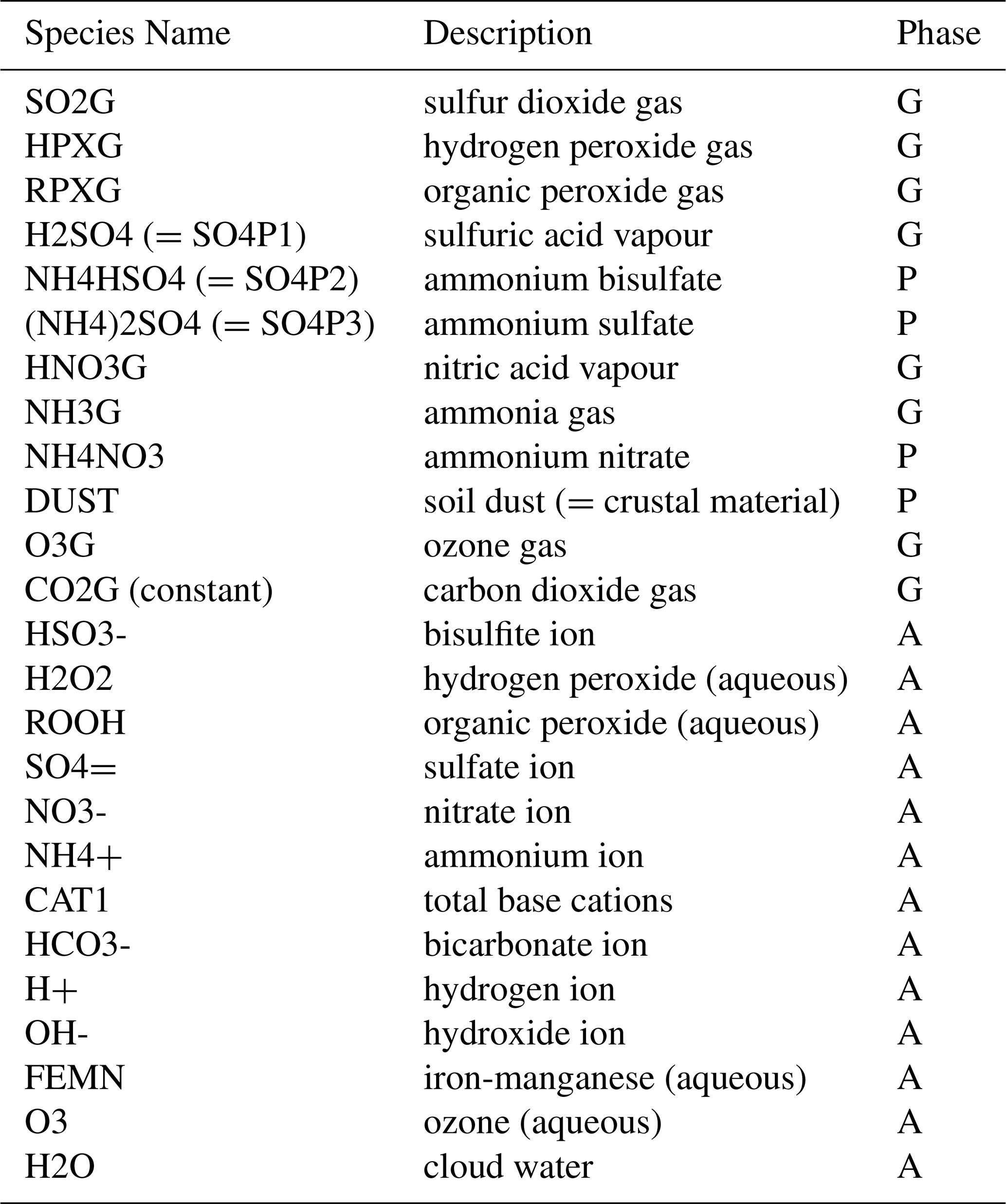
Table 7List of ADOM aqueous-phase mechanism chemical reactions, where gas-phase abundance units are ppmv and aqueous-phase concentration units are mol L−1 (see Young and Lurmann, 1984).
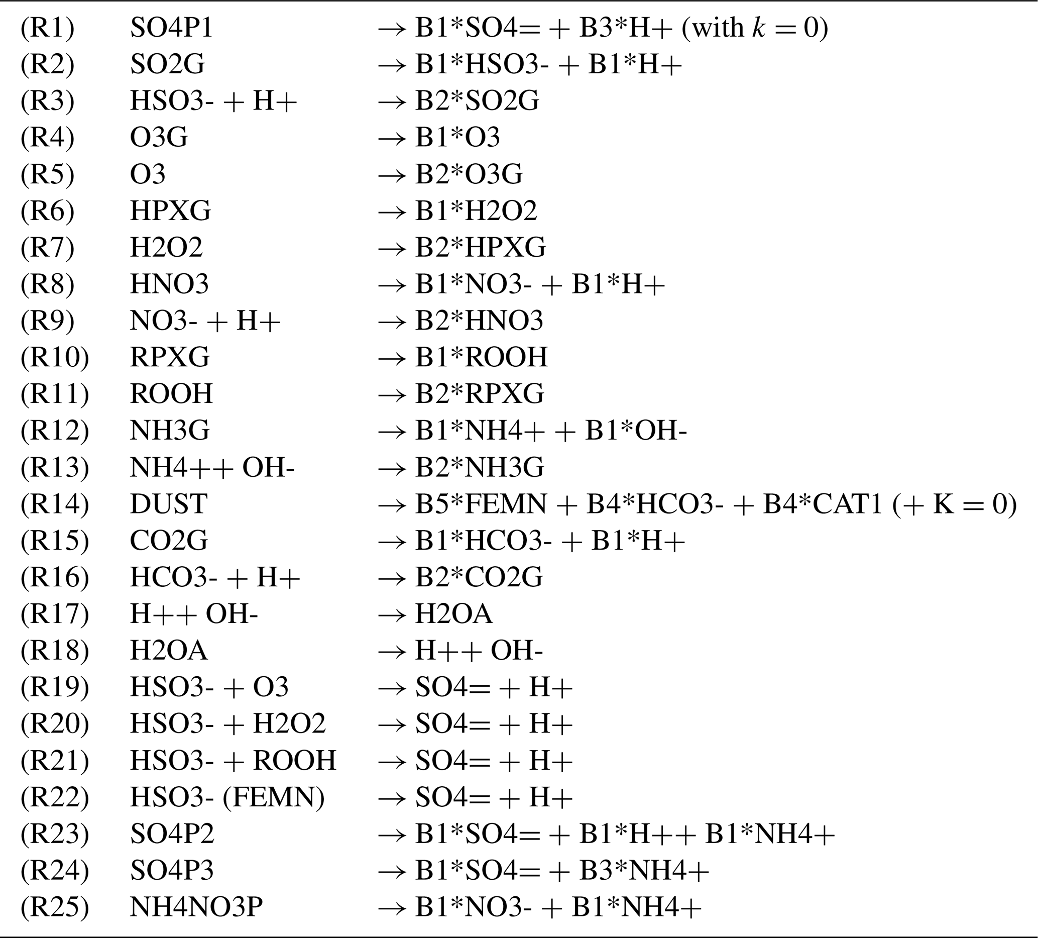
Lw= volumetric liquid water fraction in air (m3 H2O per m3 air). R= universal gas constant (8.205×10⁴ ppm L mol−1 K−1). T= dry-bulb temperature (K). k= equilibrium constant for aqueous-phase reactions. B1 =LwRT (conversion factor: gas-phase to aqueous-phase units). B2 = (LwRT)−1 (conversion factor: aqueous-phase to gas-phase units). B3, B4, and B5 are defined by the emissions data.
To reduce computer time, following Gong et al. (2006) this chemistry mechanism is implemented in MACH as a “bulk” (i.e., non-size-resolved) process that occurs in a generic cloud droplet whose size is determined from the bulk or total cloud liquid water content (LWC) supplied from GEM (Table 2) and cloud droplet number concentration Nd (Sect. 3.3.5). In addition, the GEM total cloud fraction field fcld is used to convert grid-average values to “in-cloud” values before the cloud chemistry operator is applied.
Like the gas-phase mechanism the aqueous-phase mechanism is solved for a MACH chemistry time step using the computationally efficient Young and Boris (1977) predictor–corrector algorithm with a number of smaller integration time steps. At the end of the aqueous-phase chemistry integration step, the gridded gas-phase concentrations of SO2, O3, H2O2, HNO3, ROOH, and NH3 are updated to account for their in-cloud depletion and the resulting bulk mass increments of three dissolved inorganic aerosol components (SU, NI, AM) are redistributed across activated PM size bins in air, effectively returning particle concentrations to clear air conditions. This redistribution is done by using the ratios of LWC in each activated (or partially activated) size bin to the total LWC, which implies that aqueous-phase chemistry is a volume-controlled process (Gong et al., 2006). The LWC in each bin depends on the number of activated aerosol particles in each bin and is obtained by distributing bulk LWC to all activated aerosol particles evenly (Gong et al., 2006, 2011). This mass redistribution step at the end of the aqueous-phase chemistry operator is then followed by a “rebinning” step that is needed to maintain the fixed size bin structure (Sect. 3.8). Note, however, that the resulting ambient concentrations of inorganic particle components NI and AM may not be in equilibrium with the gas phase so the inorganic heterogeneous chemistry operator is called next.
3.6 Inorganic heterogeneous chemistry scheme
Ambient sulfuric and nitric acid vapours and ammonia gas can partition to atmospheric particles to form one or more inorganic salts, and the resulting SU, NI, and AM aerosol components can make up a significant fraction of PM2.5 mass (e.g., Brook and Dann, 1999; Malm et al., 2004). Depending on the relative fractions of these three gas-phase species, four different salts may be formed (e.g., Ansari and Pandis, 1998): ammonium sulfate ((NH4)2SO4), ammonium bisulfate (NH4HSO4), letovicite ((NH4)3H(SO4)2), or ammonium nitrate (NH4NO3). Because H2SO4(g) has a very low vapour pressure (Sect. 3.3.2), it is a reasonable approximation to assume that it resides completely in the aerosol phase (Nenes et al., 1998), whereas nitric acid vapour (HNO3(g)) and ammonia gas (NH3(g)) exist in a reversible equilibrium between the gas and particle phases. Knowledge of inorganic heterogeneous chemistry thus allows the secondary inorganic component of PM to be determined.
Inorganic heterogeneous chemistry was parameterized in the RAQDPS023 version of MACH with the computationally efficient HETV (HETerogeneous Vectorized) scheme (Makar et al., 2003a), which is based on a subset of the ISORROPIA thermodynamic equilibrium algorithms (Nenes et al., 1998, 1999). In ISORROPIA the full system of inorganic equilibrium equations is broken up into subsystems, each corresponding to fixed ranges of RH and the ratio of total ammonia to total sulfate, where total ammonia includes both gas and particle forms in molar units. These ranges constrain which inorganic species (gases, ions and salts) may be present in aerosol particles. HETV considers 12 such range-based subsystems or “cases”. The multicomponent activity coefficient calculations that are required for non-ideal, high-concentration solutions use the formula of Kusik and Meissner (1978) as described by Kim et al. (1993) but are approximated using higher-order Taylor series to reduce calculation time (Makar et al., 2003a). The metastable state assumption, namely that some particle liquid water is always present even at low RH, was also made to reduce the number of cases that must be considered (e.g., Rood et al., 1989; Miller et al., 2024).
Similar to the implementation of the aqueous-phase chemistry parameterization (Sect. 3.5), HETV assumes a bulk equilibrium in the particulate phase over all particle sizes to save computer time. At the end of the inorganic-heterogeneous-chemistry integration step, gridded concentrations of HNO3(g) and NH3(g) are updated to account for inorganic gas-particle partitioning during the time step, where the updated values may have either increased or decreased. If the bulk mass increments of the three inorganic aerosol components (SU, NI, AM) are positive, then these increments are redistributed across the PM size bins. This redistribution is carried out by using the ratios of gas-phase condensation rates to all particles in a size bin based on the modified Fuchs-Sutugin equation (Hegg, 1990; Makar et al., 1998; Gong et al., 2003) and the total condensation rate summed over all size bins. If the bulk mass increments are negative, though, then mass is removed from each size bin starting with the largest based on the same condensation rate ratios. Note that it is possible that for some bins the mass that is available to be removed may be less than the pro-rated increment, in which case a second removal iteration may be required. This redistribution step is then followed by a mass-conserving “rebinning” step that is needed to maintain the fixed size bin structure (Sect. 3.8).
3.7 Secondary organic aerosol formation scheme
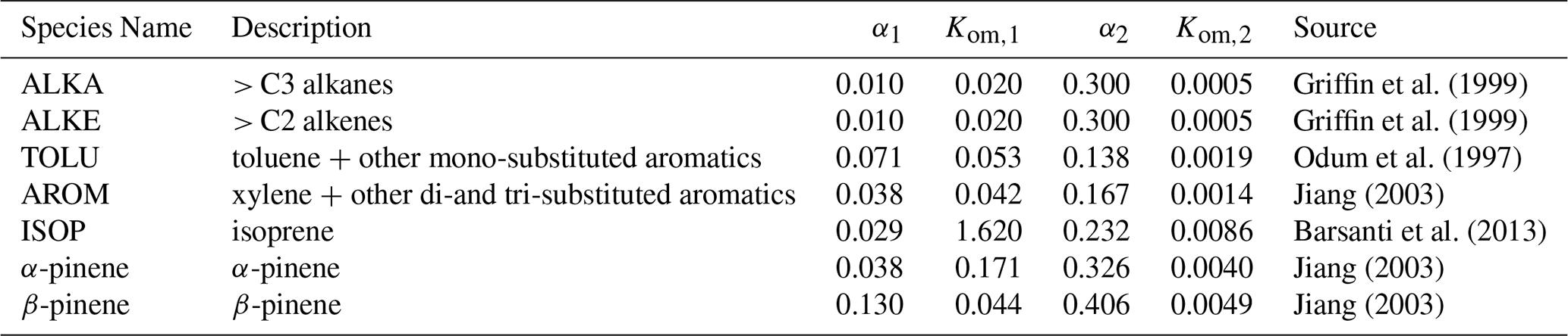
The term “secondary organic aerosol” (SOA; equivalent to SOM) refers to organic PM that results from the oxidation of gas-phase VOC precursor species followed by condensation to the particle phase (e.g., Hallquist et al., 2009; Jimenez et al., 2009). The RAQDPS023 used the Instantaneous secondary organic Aerosol Yield (IAY) scheme described by Jiang (2003, 2004, 2005) to represent SOA formation from five model VOC species. Four of these are lumped VOC species: ALKA (long-chain anthropogenic and biogenic alkanes); ALKE (long-chain anthropogenic and biogenic alkenes); AROM (multi-substituted aromatics); and TOLU (toluene and mono-substituted aromatics) (Stroud et al., 2008). The fifth model VOC species is ISOP (isoprene), which is not lumped and is dominated by biogenic emission sources (although there are also minor anthropogenic sources). The total SOA contribution from ALKE oxidation is further divided into contributions from anthropogenic ALKE and from biogenic α-pinene and β-pinene (derived from BEIS monoterpene emissions; see Sect. 3.11.3).
The Jiang scheme is based on a two-condensable-product fit to chamber data (Pankow, 1994; Griffin et al., 1999), where initial products are assumed to be converted rapidly to non-volatile organic PM. Values of the IAY parameters that were used by the RAQDPS023 are listed in Table 8, where α1i and α2i are the mass-based stoichiometric coefficients (unitless) and Kom,1i and Kom,2i are the partitioning coefficients (m−3 µg) of the ith condensable species CSi, respectively (Odum et al., 1996; Jiang, 2003). The αi and Kom,i values for ALKA and anthropogenic ALKE are taken from Griffin et al. (1999), those for AROM, α-pinene, and β-pinene are taken from Jiang (2003), the TOLU values come from Odum et al. (1997), and the ISOP values are taken from Barsanti et al. (2013).
The amount of SOA product available for condensation at each MACH chemistry time step is the sum of IAYi⋅ CSi over the seven VOC condensable species (CS) values listed in Table 8, where IAYi is a dimensionless fraction and CSi is the reduction due to oxidation of ALKA, ALKE, AROM, TOLU, and ISOP MMRs over a MACH time step as calculated by the gas-phase chemistry operator (Sect. 3.4). The condensation rate of SOA products to aerosol particles is described by a modified Fuchs-Sutugin equation (see Eq. (A14) of Gong et al., 2003), similar to the treatment for H2SO4 condensation (Sect. 3.3.2), and the relative condensation rates of H2SO4(g) to each PM size bin are used as a proxy for the relative condensation rates of these SOA organic gases. Lastly, like the H2SO4 condensation step the SOA condensation step must be followed by a “rebinning” step to maintain the fixed PM size bin structure as described next.
Table 8List of IAY parameter values for seven, SOA-forming, ADOM-2 mechanism VOC species. αi is the mass-based stoichiometric coefficient (unitless) and Kom,i is the partitioning coefficient (m−3 µg) of the ith condensable species.
3.8 Intersectional mass transfer schemes
As already noted, one complication of using a fixed sectional representation of the PM size distribution is that particles belonging to a particular size bin may grow too large for that bin due to the addition of mass from condensation or from aqueous-phase or heterogeneous chemistry (e.g., Jacobson, 1999; Gong et al., 2006). This problem can be addressed by applying a rebinning operator that partitions the enlarged particles between two adjacent size bins in a mass- and number-conserving manner in order to maintain the fixed bin structure. Jacobson (1999) refers to this rebinning approach as a quasi-stationary size structure for the PM size distribution. Interestingly, fixed modal representations of the PM size distribution suffer from an analogous issue that has an analogous solution, referred to as mode merging (e.g., Binkowski and Shankar, 1995; Binkowski and Roselle, 2003).
MACH implements a mass-conservative rebinning procedure each time step after each of three processes: condensational growth (Sect. 3.3.2 and 3.7); aqueous-phase chemistry (Sect. 3.5); and inorganic heterogeneous chemistry (Sect. 3.6). A slightly different approach to rebinning is used for each of these three processes. For condensational growth the rebinning calculation is treated as mathematically equivalent to two-particle coagulation (Gong et al., 2003). The volume of a particle in the size bin that underwent condensation (the “donor” bin) is considered to be one colliding particle while the volume of the condensable species per particle is considered to be the other colliding particle. The same formulation used by Jacobson et al. (1994, Eq. 13) to partition the volume of an intermediate particle of two coagulating particles into two model size bins (the “receiver” bins) is then used (Gong et al., 2003). The two volume partitioning factors that are calculated depend on the particle volumes of the donor and receiver size bins before condensation occurred and the particle volume for the donor bin after condensation occurred. The sum of the two partitioning factors is unity (to conserve the allocated volume), and the smaller of the two adjacent receiver size bins may be the same as the donor size bin but may also be a larger size bin (if n>2). The choice of the receiver size bins depends on the mean particle diameter diagnosed for the new total mass for the donor size bin mass after condensation using the initial donor-bin particle number. The rebinning calculations are applied to each size bin beginning with the smallest one. Note that all PM chemical components are affected by rebinning due to the assumption of internal mixing even though condensational particle growth is due only to one or two chemical components (i.e., sulfuric acid vapour or condensable organic gases).
For activated particles that have grown due to the production of particle sulfate by aqueous-phase chemistry, rebinning is performed after the redistribution step at the end of the aqueous-phase chemistry operator. A similar equivalence to two-particle coagulation is invoked, with each activated particle size bin corresponding to a donor bin and the size-bin mass gain due to cloud chemistry corresponding to the second particle, but the partitioning-factor pairs for the receiver bins are calculated with the mass-based method described by Gong et al. (2006; Eq. 3), which also conserves particle number. Rebinning is restricted to size bins with activated particles, where the rebinning calculations are applied beginning with the smallest activated or partially activated bin and then moving to successively larger activated size bins but are based on non-activated particle properties.
The inorganic heterogeneous operator is called immediately after the aqueous-phase chemistry operator (see Sect. 4.1) because the updated PM composition resulting from the latter may not be in stable equilibrium with the gas phase However, once HETV determines a new gas-particle partitioning equilibrium, some particles may have gained mass or lost mass and hence may need to be assigned to a different size bin. The mass-based method of Gong et al. (2006) is also used for rebinning here but with two adjustments. First, activation is not relevant so in the case of mass gain rebinning is applied to all particle size bins beginning with the smallest size bin and moving to successively larger bins. Second, since particles may have lost mass as well as gained mass, the two-particle coagulation analogy is generalized to account for a “donor” particle with a negative mass gain. For such negative mass increments the rebinning moves mass to a pair of smaller receiver size bins beginning with the largest size bin and moving to successively smaller bins.
The above descriptions are general and also apply to the 12-bin version of GEM-MACH. For the RAQDPS023, which only considers two PM size bins, the two adjacent receiver size bins can only be the PM2.5 and PMcf size bins and the rebinning step can only transfer particle mass from the PM2.5 size bin to the PMcf size bin. During development of the original GEM-MACH-based RAQDPS, it was found that the rebinning operator was transferring too much mass from the PM2.5 size bin to the PMcf size bin. This problem was not apparent for the 12-bin version, suggesting that the very coarse representation of the PM size distribution was introducing numerical errors. Conceptually if we consider that it is those particles whose diameters are already close to the upper end of a size bin that are most likely to grow into the next larger size bin after mass is added by condensation or other processes, then an assumption that particles of any size from the ultrafine to 2.5 µm might increase enough in size in one time step to join the PMcf size bin is unrealistic.
The solution adopted for the two-bin version to avoid this assumption was to subdivide each size bin into a number of sub-bins, allocate the mass increase for each size bin across the sub-bins, apply the rebinning operator to the individual sub-bins, and then aggregate the sub-bin particles back to the original size bins. In addition to the choice of the number of sub-bins, however, the subdivision and allocation steps could be performed in a number of ways, such as a linear vs. a logarithmic subdivision of size bins and allocation of the mass increment to a uniform distribution vs. an assumed log-normal distribution.
After some experimentation a linear subdivision of each size bin into six equal-sized sub-bins by radius was adopted with the mass of each chemical component for the size bin divided equally between the six sub-bins. For condensational growth the allocation of size-bin gained mass for a time step across the sub-bins was based on the relative fraction of total particle area by sub-bin for the size bin. For cloud chemistry the allocation step was done in three steps. First, aerosol number concentration was allocated to sub-bins based on the equal distribution of particle mass to the sub-bins. Next, cloud liquid water was allocated to each sub-bin based on the relative fraction of total particle number by sub-bin for the size bin. And third, the relative fraction of cloud liquid water by sub-bin for the size bin was used to allocate the mass increment to each sub-bin. Finally, for inorganic heterogeneous chemistry the allocation step for aerosol particle mass changes followed the approach for condensational growth: the size-bin mass increment for a time step was divided equally between the six sub-bins, but with the additional possibility that the size-bin mass increment could be negative, that is, a mass decrement, due to volatilization of the nitrate and ammonium aerosol components. The net result of introducing these modifications was to reduce the intersectional transfer of mass after these process operators from the PM2.5 bin to the PMcf bin.
3.9 Gas-phase dry deposition scheme
Many atmospheric gases, like aerosol particles (Sect. 3.3.4), are removed at the Earth's surface by dry deposition after downward transport by air motions (though gravitational settling plays no role, unlike the particle case). The rate of removal by dry deposition is determined in part by the chemical and physical properties of each individual gas, including its reactivity, solubility, and molecular diffusivity. The rate of removal is also affected by surface properties, including vegetation characteristics in the case of removal through plant stomata and by other vegetative surfaces, including wetted surfaces (e.g., Wesely and Hicks, 2000; Zhang et al., 2002b; Clifton et al., 2020, 2023; Galmarini et al., 2021).
To represent the dry deposition of gas-phase species MACH uses a variant of Wesely's resistance-analogy parameterization (Wesely, 1989), which is based on the product of the concentration of a gas-phase species at the Earth's surface and its dry deposition velocity. Following an analogy to electrical circuits, the dry-deposition velocity of a species is given by the inverse of total “resistance”, which consists of the sum of three components: aerodynamic resistance, quasi-laminar sublayer resistance, and surface resistance. Aerodynamic resistance Ra is a function of only near-surface micrometeorological conditions and the roughness characteristics of the underlying surface, so it is independent of the chemical species. Quasi-laminar sublayer resistance Rb is a function of friction velocity and the molecular diffusivity of each chemical species. The surface resistance Rc is the most important and complex resistance for most gas-phase chemical species, and it effectively determines whether a particular species is dry deposited or not. Soil resistance, soil wetness, and snow cover must be considered for all land surfaces in calculating Rc, with additional resistances (stomatal, mesophyll, cuticle, in-canopy, exposed surfaces) required in the case of vegetated surfaces (Makar et al., 2018b).
To account for the different dry deposition rates of gas-phase species, MACH considers two master species, SO2 and O3, which behave quite differently for wet surfaces (Zhang et al., 2002a, b). Weighted averages of the dry deposition velocities for these two master species are then used to scale dry deposition velocities for other dry depositing species (Zhang et al., 2002a; Makar et al., 2018b). Table 3 lists the 17 ADOM-2 gas-phase species that are dry deposited and the master-species dry deposition scaling factors (DDF) that are assumed for each. Stomatal resistance is parameterized using a one-big-leaf approach, where the effects of incoming solar radiation, temperature, and humidity deficit are empirically represented but the increase of shading due to increasing leaf area index (LAI) is neglected (Makar et al., 2018b).
One limitation of the gas-phase dry deposition scheme, however, is its simplistic treatment of vegetation phenology and seasons in both time and space: only five phenologically-based seasons are considered, which vary by month and 5° latitude bands without any dependence on longitude or elevation (Brook et al., 1999a). These seasons are used in lookup tables to specify seasonal values of a number of required parameters, including soil, cuticle, canopy, and minimum stomatal resistances, for 15 land-use types (Makar et al., 2018b). For some months, however, this treatment can result in zonal bands being visible in surface concentration fields due to seasonal differences between latitude bands. Two removal processes for SO2 were also recently identified as missing from the RAQDPS023: the soil-wetness and cuticle-wetness gas-phase dry deposition pathways (e.g., Wesely, 1989; Galmarini et al., 2021; Clifton et al., 2023). Further details about the scheme used by MACH to model the dry deposition of gases may be found in Makar et al. (2018b), and evaluation results for O3 deposition for this scheme and for comparable schemes used by other CTMs can be found in three recent papers (Clifton et al., 2023; Hogrefe et al., 2025; Kioutsioukis et al., 2025).
3.10 Wet deposition schemes
Wet deposition, which is also referred to as wet removal or precipitation scavenging, consists of multiple processes related to tracer scavenging and transport by hydrometeors, which may have the form of raindrops, snowflakes, ice pellets, graupel, or hail (e.g., Slinn, 1984; Seinfeld and Pandis, 2016). Some wet deposition processes act within clouds while other wet deposition processes act below clouds. The former are referred to as in-cloud scavenging or “rain-out” while the latter are referred to as below-cloud scavenging or “wash-out”. “Snow-out” must also be considered, and, unlike raindrops, solid hydrometeors can have many shapes or habits, including plates, needles, dendrites, and columns (e.g., Slinn, 1984; Zhang et al., 2013). As well, the processes responsible for the removal of soluble gases vs. aerosol particles are not identical. But regardless of these complexities, a number of modelling studies have suggested that wet deposition can be the dominant removal pathway for aerosol particles, though not for soluble gas-phase species (e.g., Barrie et al., 2001; Iversen and Seland, 2002; Textor et al., 2006).
As described in Sect. 3.3.5 aerosol particles that are activated in the supersaturated conditions within clouds act as CCN and become cloud droplets. Soluble gases inside clouds may also enter cloud droplets through gas-particle partitioning (Sect. 3.5). The majority of clouds are non-precipitating, but if cloud droplets do form raindrops that then fall from the cloud, both dissolved particle mass and dissolved gases from the cloud layer are also carried downwards by the raindrops. This “rain-out” process is parameterized in MACH using both bulk autoconversion (or precipitation production or cloud-to-rain conversion) rate fctr obtained from GEM (ppro in Table 2; see Eq. (5) of Gong et al., 2006) and SGS convective precipitation production from the middle and deep convection implementations of the Kain-Fritsch scheme (Sect. S1.7). The GEM total cloud fraction field fcld (ftot in Table 2) is then used to convert grid-averaged parameters (e.g., cloud liquid water content, precipitation rates/fluxes) for each model layer to “in-cloud” values (Gong et al., 2006). The contribution of mid-level SGS convective precipitation to precipitation scavenging was added in MACH for the RAQDPS023 (Moran et al., 2021b). Note that the “snow-out” process within cold clouds consisting of ice crystals is not considered explicitly by MACH (Gong et al., 2006).
Falling hydrometeors can also scavenge aerosol particles and soluble gases located below cloud base (e.g., Slinn, 1984; Gong et al., 2006; Wang et al., 2010; Zhang et al., 2013). To calculate the below-cloud scavenging of aerosol particles by liquid or solid precipitation, MACH follows CAM (Gong et al., 1997a, 2003; Gong et al., 2011; Ghahreman et al., 2024) and employs a simplified treatment of the particle-size-dependent precipitation scavenging rate coefficient Λ(d) proposed by Slinn (1977, 1984), where d is the particle diameter. This includes a semi-empirical expression for the collection efficiency E(d,D), where D is a characteristic size of the hydrometeor, that accounts for the three dominant particle collection mechanisms (Brownian diffusion, interception, inertial impaction) and assumes that the retention efficiency is unity (Slinn, 1977, Eq. 10). In the case of rain, D corresponds to the diameter of a spherical raindrop, the particle settling velocity is neglected relative to the raindrop terminal fall speed Vrt, and the precipitation number distribution is assumed to be monodisperse and characterized by a mean raindrop diameter Dm that can be calculated from the precipitation rate p (Slinn, 1977, Eq. 14). Vrt is calculated using a formula from Beard (1976). Dm and Vrt are then used with Eq. (10) of Slinn (1977) to calculate the mean collection efficiency ), which is used in turn to calculate Λr(d), the particle-size-dependent rate coefficient for rain scavenging. Λr(d) depends directly on p and ) and inversely on Dm (Slinn, 1977, Eq. 13).
A similar formulation is used by MACH to parameterize below-cloud scavenging of particles by snow, but the precipitation rate p corresponds to a rainwater equivalent (snow density is assumed to be a factor of 10 less than rain) and the mean collection efficiency depends on l, a characteristic dimension of the solid hydrometeors for particle collection that may be different from D, the size of the hydrometeors. The resulting snow scavenging rate coefficient Λs(d) depends directly on p and and inversely on Dm (Slinn, 1984, Eq. 11.36). The frozen hydrometeor terminal fall speed Vst needed to calculate is obtained using the parameterization of Slinn (1984) (see also Gong et al., 1997a). Slinn (1984) suggested Dm values for five different snow habits, of which MACH considers snow scavenging for three different temperature ranges by needle snow (−8 to 0 °C), stellar snow (−25 to −8 °C), and graupel ( °C) (Gong et al., 2011).
Below-cloud scavenging is assumed to be due to a single precipitation phase, either rain or snow. A threshold of the ambient dry-bulb temperature T is used to determine the phase: rain for T>0 °C and snow for T < 0 °C (Ghahreman et al., 2024). To account for wet removal of particles in the partial vertical column below cloud base, a two-dimensional cloud cover field is first calculated from the three-dimensional total cloud fraction field fcld using a random overlapping algorithm (Mailhot et al., 1998). This two-dimensional cloud cover field is then used to convert grid-averaged parameters (e.g., precipitation rate) into separate below-cloud and clear-sky values and then to recalculate grid-averaged values (Gong et al., 2006).
Six soluble gases (SO2, HNO3, NH3, H2O2, ROOH, CO2) are also removed in MACH by below-cloud precipitation scavenging. The removal of HNO3, NH3, H2O2, and ROOH is treated as an irreversible process similar to particle scavenging. This is a reasonable assumption when the ambient concentration of the gas-phase species is much greater than its equilibrium concentration at the surface of the raindrop or if the effective Henry's law coefficient for the species is very large (e.g., Seinfeld and Pandis, 2016). Λi, the scavenging rate coefficient for rain for the ith gas species, is calculated using Eqs. (6) and (7) of Gong et al. (2006), where the four key parameters are p, Dm, Vrt, and Di, the gas-phase diffusivity of the ith species. Wet scavenging of SO2 and CO2, on the other hand, is treated as a reversible process since their gas-phase and gas-droplet equilibrium concentrations may be closer in magnitude or their effective Henry's law coefficient is not large. The two equilibrium equations given by Eq. (8) of Gong et al. (2006) are used for these two species, where the key parameter is H′, the effective equilibrium constant that combines absorption and dissociation equilibria. Lastly, scavenging of soluble gases by snow and ice is only considered for HNO3 and NH3. This process is assumed to be irreversible and is based on scaling the H2SO4 scavenging rate (Karamchandani et al., 1985; Gong et al., 2006).
While wet deposition results from hydrometeors transporting pollutants downwards to the Earth's surface where they are removed, some hydrometeors may evaporate before they reach the ground, in which case the pollutants are released back to the ambient air, though at a lower elevation. This vertical transport process is explicitly included in MACH (see Gong et al., 2006) by using the precipitation evaporation rate predicted by GEM (pevp in Table 2). Pollutants are assumed to be released from evaporating hydrometeors at the same rate as water vapour.
3.11 Chemical emissions inputs
Files of gridded chemical emission fluxes are a key input to CTMs, and they have a direct and large impact on model performance. In effect these emission fluxes constitute a chemical forcing term that transforms the chemical-species mass conservation equations of a CTM from an initial-value problem into an initial-boundary value problem. However, the preparation of these emission fluxes into a model-ready form is a challenging task. For one thing, all sources of emission fluxes must be considered, including both anthropogenic and natural emissions. In addition, extensive pre-processing is required to prepare files of anthropogenic emission fluxes before a CTM simulation can be performed whereas natural emissions are typically not known in advance and must be modelled and predicted during a CTM simulation.
A new set of gridded, hourly anthropogenic emissions flux input files for each month of the year for a typical seven-day week was generated for use by the RAQDPS023 and RAQDPS-FW023 (Moran et al., 2021b; see also Table A1). This emissions data set is referred to as SET4.0.0. This section describes the data sources and the preparation of the SET4.0.0 data set along with the modelling of biomass burning emissions, biogenic emissions, and sea-salt emissions.
3.11.1 Anthropogenic emissions
Information about year-specific anthropogenic emissions for North America for use by CTMs is usually obtained from available annual national emissions inventories (e.g., Miller et al., 2006; Moran et al., 2013; Day et al., 2019; Foley et al., 2023). Such inventories are most often compiled by government agencies. The following three annual national anthropogenic emission inventories were used as the basis for generating the SET4.0.0 emissions input files:
-
Projected 2020 Canadian Air Pollutant Emissions Inventory (APEI) based on the 2015 APEI (ECCC, 2016; Sassi et al., 2021);
-
Projected 2023 U.S. National Emissions Inventory (NEI) based on version 1 of the U.S. Environmental Protection Agency (EPA) 2016 Emissions Modeling Platform for policy development applications (U.S. EPA, 2019); and
-
Projected 2023 Mexican NEI based on 2008 Mexican NEI (U.S. EPA, 2019, p. 168).
Each of these inventories contains annual or monthly emissions of seven criteria air contaminants (CACs), namely SO2, NOx, CO, VOC, NH3, PM2.5, and PM10, reported for different emission source sectors (e.g., heavy-duty diesel vehicles, residential wood combustion, solvent use, agricultural tillage, etc.) by subnational jurisdiction. Emission source sectors corresponding to 417 Source Classification Codes (SCCs) were contained in the 2020 Canadian inventory vs. 5473 SCCs for the 2023 U.S. inventory and 791 SCCs for the 2023 Mexican inventory, while Canadian emissions were reported for 13 provinces and territories vs. 3249 counties for the U.S. and 2457 counties for Mexico (CMC-RAQDPS-023, 2021). It should be noted that the level of detail or granularity of emissions reporting in each inventory affects the level of detail that can be employed for subsequent emissions processing (see Sect. S2). For example, the county-level reporting of emissions for the U.S. and Mexico vs. province-level reporting for Canada meant in effect that some spatial allocation had already been performed for the U.S. and Mexico. Note too that not all U.S. and Mexican counties were located within the RAQDPS023 model domain, which meant that these emissions were not included in the SET4.0.0 files.
Most emissions inventories are retrospective (i.e., historical) because their preparation requires the use of year-specific annual activity data such as the amount of fuel combusted or vehicle kilometers travelled in the inventory base year, and such activity data will only be available sometime after the end of the base year. Projected (or future-year) emissions inventories, on the other hand, are prospective (i.e., forecasts) because they are generated by “projecting” the emissions from a retrospective base inventory forward in time to a future year based on a set of assumptions about expected future changes to the economy, population and housing, on-road and off-road vehicle fleets, etc. along with information about any emissions changes that are expected to result from the phased implementation of existing emissions control legislation. When annual emissions levels are changing rapidly, the use of a retrospective inventory may not represent current emission levels as well as a projected inventory despite the greater uncertainties associated with a projected inventory due to the additional assumptions involved in its generation (e.g., Pan et al., 2014; Moran et al., 2020a). This was the reasoning used to choose each of the three projected future-year emission inventories listed above (in addition, importantly, to their availability): the RAQDPS023 became operational in 2021 at a time when the most recent available retrospective national emissions inventories were for base years 2015 or 2016 whereas overall North American emissions had been trending downwards for more than two decades (e.g., ECCC, 2022b; https://gispub.epa.gov/air/trendsreport/2021, last access: 18 March 2026).
After special emissions-processing-ready versions of the three projected annual national anthropogenic emissions inventories had been generated by ECCC for Canada and acquired for the U.S. and Mexico (U.S. EPA, 2019), they underwent extensive processing to prepare the SET4.0.0 emissions input files. As described in Sect. S2 the first step was to make some adjustments to the Canadian and U.S. inventories to account for additional and missing information. The inventories were then read by the SMOKE (Sparse Matrix Operation Kernel Estimation) emissions processing system (see https://www.cmascenter.org/smoke/, last access: 18 March 2026) to prepare the model-ready SET4.0.0 input emissions files. More details about this demanding and time-consuming task can be found in Sect. S2.1.
Table 9 compares the annual totals of model-ready anthropogenic emissions of the seven CAC species by country. These values were obtained from the full set of SET4.0.0 emissions files. It is clear from Table 9 that total U.S. emissions are larger than either Canadian or Mexican total emissions, but the relative size of the national emissions for the three countries depends on the pollutant species. For example, U.S. SO2 emissions are twice as large as Canadian SO2 emissions and U.S. NOx emissions are four times larger than Canadian NOx emissions, but U.S. emissions for the other five CAC species are all larger than the corresponding Canadian emissions by a factor of six or more. Interestingly, NOx emissions from ocean shipping are comparable to land-based Canadian and Mexican NOx emissions. Note too that this summary is based on SMOKE outputs and hence does not agree exactly with inventory totals (cf. Table 1 of the companion paper by Moran et al., 2026). One source of these differences is that the model domain does not contain all inventory emissions. This is especially true for Mexico, for which only 340 of Mexico's 2457 counties are completely or partially included in the model domain, but also applies to the U.S., for which 105 counties, including the state of Hawaii, and overseas territories such as Puerto Rico, the U.S. Virgin Islands, Guam, and American Samoa, are located outside of the model domain although their emissions are included in the U.S. NEI. Another source of these differences is the VOC definition: VOC in Table 9 is the sum of the emissions of the 11 model reactive VOC species (i.e., post-SMOKE) whereas VOC in Table 1 of Moran et al. (2026) corresponds to the bulk VOC emissions reported in the inventories, including unreactive species (i.e., pre-SMOKE). Third, the PM emission values in Table 9 are much lower than in the inventory totals in the other table because they have been reduced by scaling with the transportable-fraction (TF) factor to account for SGS removal processes after emission (Pace, 2005).
Table 9Summary of annual, model-ready Canadian, U.S., and Mexican anthropogenic emissions and ocean shipping emissions (tonnes) for nominal 2021/22 period based on the SET4 emissions input files. Note that (i) inventory emissions from jurisdictions located outside of the model domain (e.g., southern Mexico, Hawaii, Puerto Rico) are not included in these totals, (ii) VOC emissions are calculated as the sum of the emissions of 11 model VOC species (excludes EOTH), (iii) fugitive PM2.5 and PM10 emissions have been reduced by transportable-fraction scaling but not by meteorological modulation, and (iv) in-flight aircraft, biogenic, biomass burning, lightning, volcanic, sea-salt, pollen and other biologicals, and aeolian dust emissions are not included.
Figure 3 shows the spatial distribution across the RAQDPS023 domain of mean July SET4.0.0 anthropogenic emissions of four chemical species: NO, VOC, NH3, and PM2.5. These spatial distributions are quite different due to variations in the relative contributions of different emissions source types for each species. For example, the contribution of ocean-going vessels to NO and PM2.5 emissions is obvious in Figs. 3a and d. NO emissions are also associated with urban areas, highways, power plants, and agriculture. The spatial distribution of NH3 emissions, on the other hand, is dominated by the agricultural sector, including fertilizer application for field crops and animal husbandry, which includes farm-level emissions but also concentrated animal feeding operations located in rural areas.
Figure 3Spatial distribution of SET4.0.0 July anthropogenic emission of four chemical species: (a) NO (tonnes NO per grid cell), (b) VOC (tonnes VOC per grid cell), (c) NH3 (tonnes NH3 per grid cell), and (d) PM2.5 (tonnes PM2.5/grid cell). Note that “VOC” here is total model VOC, that is, the sum of the 11 emitted model VOC species (see Table 3), and PM2.5 emissions are the sum of emissions of the six emitted PM2.5 chemical components (SU, NI, AM, EC, POM, and CM).
3.11.2 Biomass burning emissions
Wildfires and other biomass burning (BB) sources such as prescribed burns can emit large quantities of atmospheric pollutants, including PM2.5, NOx, CO, VOC, and NH3, and sometimes occur over many days in the case of long-lived fires (e.g., Akagi et al., 2011; Urbanski, 2014). In addition to their significant local impacts, smoke from wildfires can also be transported hundreds or even thousands of kilometres downwind (e.g., Jaffe et al., 2004; Pavlovic et al., 2016; Teakles et al., 2017). About 39 % of Canada and 34 % of the U.S. are covered by forest (https://data.worldbank.org/indicator/, last access: 18 March 2026), so wildfires started by lightning strikes or human activity are common in both countries (e.g., https://ciffc.ca/publications/canada-reports, last access: 18 March 2026; https://www.ncei.noaa.gov/access/monitoring/monthly-report/fire/, last access: 18 March 2026). Wildfires occur sporadically, however, and their initiation and evolution are difficult to predict. Moreover, wildfire emissions depend on many factors, including fire location, availability and condition of fuel, and past and current weather. Thus, in order to quantify and incorporate wildfire emissions into a CTM, wildfires occurring even in remote locations must be detected in near real time and their future hourly emissions predicted by the modelling system.
In 2013 ECCC, in collaboration with the Canadian Forest Service (CFS) and with contributions from the U.S. Forest Service (USFS), began to run an experimental version of the RAQDPS named FireWork, which was identical to the operational RAQDPS except for the addition of hourly BB emissions to the usual hourly anthropogenic emissions and the inline biogenic and sea-salt emissions (described in the next section). The BB emissions were calculated by combining NRT satellite-derived “hotspot” locations with estimates of fuel moisture, total fuel consumption, and fraction of smoldering vs. flaming combustion at these locations. This information was provided by the CFS Canadian Wildland Fire Information System (CWFIS), with hourly BB emission estimates produced using the Fire Emission Production Simulator (FEPS), a component of the USFS's BlueSky Modeling Framework (Lee et al., 2002; Anderson et al., 2004; Larkin et al., 2009; Pavlovic et al., 2016; Munoz-Alpizar et al., 2017). The CWFIS tracks current fire danger conditions and fire activity and characteristics across Canada and the U.S. (https://cwfis.cfs.nrcan.gc.ca/, last access: 18 March 2026), while FEPS manages data concerning fuel type, pollutant emission factors, and heat release characteristics of individual BB events (https://research.fs.usda.gov/pnw/products/dataandtools/fuel-and-fire-tools-fft, last access: 18 March 2026). Note that we refer here to BB emissions rather than wildfire emissions because of the possibility that large grass fires and prescribed burns may also be detected by satellite.
FireWork was then introduced operationally by ECCC in 2016 as a nearly identical copy of the RAQDPS, that is, identical except for the inclusion of NRT satellite-derived BB emissions (Munoz-Alpizar et al., 2017). Running these two very similar forecast systems allowed wildfire plumes to be identified by their PM2.5 concentration (referred to as “fire-PM2.5”), which were calculated by “brute force” as the difference between the FireWork and RAQDPS PM2.5 fields. The hourly evolution of these smoke plumes could then be predicted and displayed (Pavlovic et al., 2016; https://weather.gc.ca/firework/index_e.html, last access: 18 March 2026). FireWork then underwent a number of upgrades after 2016 (see Table A1), including the implementation of the Canadian Forest Fire Emissions Prediction System (CFFEPS). CFFEPS incorporates the code for the CWFIS while introducing a more flexible and updateable alternative to the FEPS module along with a new fire plume-rise scheme (Chen et al., 2019a, b). Section S3 describes CFFEPS version 4.1 and the calculation of NRT BB emissions by the RAQDPS-FW023, the formal name of FireWork v023, which was implemented operationally at the same time as the RAQDPS023 (Chen and Menelaou, 2021).
3.11.3 Other natural emissions
Two other important sources of natural emissions are soil and vegetation (e.g., biogenic emissions) and the oceans (e.g., sea-salt emissions). Both of these sources of emissions were represented in the RAQDPS023 by emissions models.
Vegetation naturally releases numerous VOCs to the atmosphere as a byproduct of photosynthesis and other plant physiological processes (e.g., Fehsenfeld et al., 1992; Monson et al., 1995; Fuentes et al., 2000; Guenther et al., 2000). Many of these compounds, such as isoprene, monoterpenes, sesquiterpenes, and aldehydes and other oxygenated VOCs, are reactive and thus can influence atmospheric chemistry (e.g., Guenther et al., 2000; Duhl et al., 2008). Moreover, globally and in many regions, including eastern North America, these biogenic VOC emissions are larger in magnitude in total than anthropogenic VOC emissions (Roselle et al., 1991; Guenther et al., 1995, 2000; Pierce et al., 1998). Emissions of NO from microbial processes in certain soil types are a second type of biogenic emission (Williams et al., 1992a, b; Yienger and Levy, 1995; Stohl et al., 1996; Guenther et al., 2000). Soil NO emissions tend to occur in rural regions, where other anthropogenic sources of NO are small, and especially in agricultural areas where nitrogen fertilizer is applied since soil nitrogen availability is a controlling factor (Sha et al., 2021).
To calculate biogenic emissions at each chemistry time step the RAQDPS023 employed inline code based on a modified version of the Biogenic Emission Inventory System (BEIS) version 3.09, which was developed by the U.S. EPA (Vukovich and Pierce, 2002), together with a modified version of the Biogenic Emissions Landuse Database version 3 (BELD3), a North American vegetation database (Pierce et al., 2000; Zhang et al., 2018), and meteorological fields predicted by GEM. BEIS v3.09 calculates the emissions of four chemical species or groups of species – isoprene; monoterpenes; “other VOCs” (OVOC); and soil NO – using formulas from Geron et al. (1994). To save computer time, gridded summer and winter standard emissions fluxes (unit: g s−1 grid cell−1) were pre-calculated for standard mid-day meteorological conditions (ambient temperature of 30 °C, photosynthetic active radiation (PAR) photon flux density of 1000 µmol m−2 s−1) by summing vegetation-species-specific emission fluxes weighted by the vegetation-species fraction for each model grid cell (Geron et al., 1994; Guenther et al., 1994; Pierce et al., 1998). Winter emission fluxes for deciduous species were assumed to be zero. These standard biogenic emission flux fields were then treated like other time-independent geophysical fields and were input at the start of a RAQDPS023 simulation. A season-specific standard emission flux for each grid cell was then calculated during a simulation as the weighted average of the summer and winter standard emission fluxes using one of the following pairs of weights for the five phenological seasons of Zhang et al. (2002a): , , , , and for midsummer, autumn before harvest, autumn after harvest, winter, and spring seasons, respectively (cf. Sect. 3.9). The phenological season for each grid cell was determined based on the month and latitude (Brook et al., 1999a). GEM-predicted air temperature and solar angle fields were then used at each chemistry time step to calculate a light correction factor for isoprene and temperature correction factors for all three VOC species and soil NO. These correction factors accounted for the difference between the actual meteorological conditions and the standard meteorological conditions and were used to scale the season-specific standard biogenic emission fluxes. Lastly, emissions of the first two VOC species and soil NO were mapped directly to three ADOM-2 model species (ISOP, ALKE, and NO) while emissions of OVOC were split equally between ALKA and ALKE.
Note that three major updates were made to the standard BEIS v3.09 system described by Vukovich and Pierce (2002). First, the v3.09 biogenic emission factors have been replaced by newer BEIS v3.13 emission factors (Schwede et al., 2005). Second, standard emission fluxes for monoterpenes and OVOC were reduced for all pine species by factors of roughly five and two, and for all spruce species by factors of roughly five and three, as suggested by Stroud et al. (2010). And third, the original BELD3 vegetation database was updated over Canada to replace the three generic forest types (coniferous, deciduous, mixed) that had been specified for Canada with 30 BELD3 tree species based on the 2001 Canadian Forest Inventory (Beaudoin et al., 2014). One remaining limitation, however, that was addressed in later versions of BEIS was that soil NO emissions did not depend on soil moisture or precipitation (cf. Yienger and Levy, 1995).
The generation of sea spray aerosol over the world's oceans is an important PM source (e.g., De Leeuw et al., 2011). These sea-salt particles have a major influence on marine cloud properties and the radiation balance over the oceans, as well as coastal areas. A number of semi-empirical schemes are available for estimating sea-salt emission fluxes, but their estimates of these emissions at the global scale can vary by nearly two orders of magnitude (Textor et al., 2006; De Leeuw et al., 2011). One reason for this large uncertainty is the need for commonality in terms of assumed RH, reporting height, and particle size range.
Two schemes for sea-salt emission fluxes from the open ocean are available in MACH: the Smith et al. (1993) scheme, which is applicable to particles with wet diameters (RH = 80 %) in the 2 to 40 µm range, and the Gong-Monahan scheme (Gong, 2003), which is applicable to particles with wet diameters (RH = 80 %) in the 0.14 to 40 µm range. A third scheme for estimating sea-salt emission fluxes in the near-shore surf zone based on a single power law is also available in the model (De Leeuw et al., 2000, Eq. 4). This simple scheme is applicable to particles with wet diameters (RH = 80 %) in the 1.6 to 20 µm range. Note that sea-salt particles are assumed to equilibrate instantaneously with the ambient water vapour in all three schemes (Fitzgerald et al., 1998). As well, all three schemes are formulated in terms of 10 m wind speed and describe the dependence of particle number flux at 10 m height on wet particle size (RH = 80 %), which must then be used to calculate integrated dry particle mass flux estimates across each model size bin. Note that De Leeuw et al. (2011) suggest that sea-salt particle diameters at RH = 80 % are roughly double their diameters at RH = 0 %.
The RAQDPS023 used the latter two schemes, where the Gong-Monahan scheme was applied for any grid cell that includes at least some ocean while the surf zone scheme was used when the fraction of a grid cell covered by ocean was less than unity. For both schemes the resulting sea-salt emission flux estimates were scaled for each grid cell by the fraction of ocean coverage. Lastly, to calculate sea-salt emission fluxes for the two RAQDPS023 size bins, each bin was subdivided into 35 sub-bins in order to integrate the particle-size-dependent emission flux functions by particle radius.
Note, however, that some other sources of natural emissions, including lightning NO emissions, volcanic SO2 emissions, pollen and other biological PM emissions, oceanic gas-phase emissions, and aeolian dust emissions, were not considered by the RAQDPS023. While all of these emissions affect atmospheric chemistry, their impacts on near-surface gas-phase and PM2.5 concentrations over Canada are assumed to be small, especially when compared to biogenic, biomass burning, and sea-salt emissions, the three types of natural emissions that are considered. Lightning NO emissions occur intermittently above the Earth's surface. While they have little influence on surface concentrations locally, they can influence NO wet deposition (e.g., Appel et al., 2011; Zhang et al., 2018b). Volcanic SO2 emissions can affect atmospheric concentrations and deposition, but active volcanoes are not a significant source in populated areas of Canada or the U.S. although this is not true in Mexico (e.g., Fioletov et al., 2016). Pollen and other biological PM emissions are an important source of atmospheric PM and aeroallergens, but they are present mainly as particles larger than 2.5 µm in diameter, including pollen grains, which are typically larger than 20 µm, and fungal spores, which are typically found in the 1–10 µm range (e.g., Efstathiou et al., 2011; Sierra-Heredia et al., 2018; Subba et al., 2021). Oceanic emissions of gas-phase species such as DMS and isoprene contribute to background atmospheric chemistry, although DMS emissions are small at higher latitudes and marine isoprene emissions are small compared to terrestrial emissions (e.g., Bates et al., 1992; Khan et al., 2025). However, as discussed in Sect. 6.2 emissions of halogen species such as iodine can affect surface ozone levels. Aeolian dust emissions are discussed further in Sect. 3.12, but such emissions are very sporadic and are much less important in Canada than the U.S.
3.12 Meteorological modulation of fugitive PM emissions
Anthropogenic fugitive PM emissions are incidental soil dust emissions that originate from surface sources such as vehicles travelling on paved or unpaved roads and a number of industrial, construction, and agricultural activities like land-clearing, excavating, grading, demolition, tilling, and harvesting. The dominant chemical components of fugitive PM emissions are CM and POM (e.g., Boutzis et al., 2020). These emissions make up a major fraction of the anthropogenic primary PM emissions considered by regional AQ models. For example, in the 2020 Canadian APEI, fugitive dust emissions contributed 88 % of total primary PM2.5 emissions and 94 % of total primary PM10 emissions (ECCC, 2022a).
Unlike primary PM emissions from smokestacks and tailpipes (i.e., combustion processes), fugitive PM emissions can be directly affected by meteorological conditions since soil wetness or snow cover may reduce fugitive PM emissions. To account for such meteorological “modulation”, hourly inventory-based fugitive PM emissions were reduced in the RAQDPS023 at each time step during a model simulation according to predicted meteorological conditions in a surface grid cell if one of the following two meteorological thresholds was exceeded:
- i.
grid-scale soil moisture (soil volumetric water content) greater than 10 %; or
- ii.
grid-scale snow depth greater than 5 cm.
If either threshold was exceeded, then fugitive PM emissions from that grid cell for that time step were set to zero for all PM size bins and chemical components. This scheme was thus most active during rainy seasons and in winter. Note that in order to apply this scheme, input PM surface emissions had to have been separated and saved as non-fugitive and fugitive components when they were generated (see Sect. S2).
The choice of 10 % for the grid-scale soil wetness threshold was made based on sensitivity tests for several trial values followed by comparison of predicted near-surface CM concentrations with CM values measured in one Canadian and two U.S. PM2.5 speciation networks (NAPS, CSN, IMPROVE). The U.S. operational AQ forecast system, the National Air Quality Forecast Capability (NAQFC), also applies a similar reduction of fugitive dust emissions by scaling PM emission fluxes by snow-cover fraction (Lee et al., 2017).
Note that this meteorological modulation scheme, which accounts for day-specific reductions of anthropogenic fugitive dust emissions by precipitation and snow cover, was independent of the land-cover-dependent TF scaling that was applied to anthropogenic fugitive dust emissions at the end of emissions processing (see Sect. S2). It should also be noted that natural aeolian (i.e., wind-blown) fugitive dust emissions, which were not considered by the RAQDPS023, can be important in arid or semi-arid parts of North America such as the desert southwest of the U.S. Such emissions are very episodic, however, and tend to occur in the spring and summer seasons under dry and very windy conditions (e.g., Orgill and Sehmel, 1976; Park et al., 2007; Foroutan et al., 2017; Kim et al., 2021). Nevertheless, these natural emissions may contribute over 50 % of PM2.5 mass in the spring season in the southwestern U.S. and 20 %–30 % of PM2.5 mass in the summer in the central and southeastern U.S. (e.g., Orgill and Sehmel, 1976; Hand et al., 2017; Tong et al., 2023), and the operational U.S. NAQFC does include an aeolian dust emissions scheme (Dong et al., 2016; Campbell et al., 2022).
3.13 Plume rise and vertical spread
Emissions from large smokestacks may disperse in the atmosphere quite differently from surface emissions. Such continuous pollutant plumes can rise well above the top of the emitting smokestack (plume rise) and then, depending on atmospheric vertical stability, display a number of types of dispersive behaviour, including coning, looping, fanning, lofting, and fumigating (e.g., Pasquill and Smith, 1983). Plume rise also exposes these pollutant plumes to different meteorological conditions at different elevations, including differing wind speeds and directions (referred to as vertical wind shear).
Pollutant point sources for which plume rise is modelled are often referred to as major point sources. In order to calculate plume rise, four major-point-source characteristics (known as stack parameters) are typically required: geometric stack height; geometric stack exit diameter; pollutant stack exit temperature; and pollutant stack exit flow speed (or stack volume flow rate). Major-point-source emissions were read by the RAQDPS023 from a separate file that also included stack-parameter values for each major point source (see Sect. S2). Information was also needed about atmospheric conditions at each stack location, including the vertical temperature profile, wind speed at the stack exit, PBL height, Monin-Obukhov length, and friction velocity. These values were all forecast by the GEM model (Table 2).
To calculate plume rise and vertical spread the RAQDPS023 employed a set of empirical formulations developed by Briggs (1984) that consider both buoyancy- and momentum-driven processes. Vertical spread represents the impact of SGS vertical diffusion associated with the mixing of the plume with its surrounding environment; it was expressed in the RAQDPS023 in terms of the vertical layers into which the emitted pollutant is injected. The implementation of the Briggs scheme in the RAQDPS023 has been described in detail by Akingunola et al. (2018). Note, though, that plume rise associated with wildfire plumes was treated differently (Sect. S3)
While the Briggs (1984) scheme provides estimates of mean injection height and plume vertical spread, one limitation of the treatment of major point source emissions by GEM-MACH (and other Eulerian CTMs) is that instantaneous horizontal and vertical mixing is assumed across the horizontal grid cell in which the point source is located and the vertical layers into which the pollutant is injected. This assumption usually has a minor impact on the far-field dispersion of the plume, but it does overestimate near-field plume diffusion and also changes plume chemistry by removing the distinction between SGS pollutant concentrations inside and outside of the plume. Note that a number of SGS plume-in-grid schemes have been proposed to address this limitation (e.g., Mathur et al., 1992; Kumar and Russell, 1996; Karamchandani et al., 2011), but the RAQDPS023 did not account for SGS plume chemistry.
4.1 Time integration
For the time integration of a GDPS, RDPS, or RAQDPS simulation, time-stepping calculations start with the GEM dynamical core (Sect. S1.1). After the calculations for a dynamics time step have been completed, the GEM “physics” module (e.g., Mailhot et al., 1998; McTaggart-Cowan et al., 2019a) is then called to step through a set of parameterization schemes representing different atmospheric physical processes. Changes to GEM state variables that result from each physical process parameterization (i.e., tendencies) are treated by GEM as forcings that modify the dynamical equations using the sequential tendency-splitting technique for physics-dynamics coupling discussed by Gross et al. (2018). One exception, though, is the atmospheric radiative transfer scheme, which is computationally expensive and which, in both the RDPS 8.0.0 and RAQDPS023, was only called every fifth dynamic time step (i.e., every 1500 s).
In a GEM-MACH simulation the MACH module is called upon completion of the GEM physics module. In order for the RAQDPS023 to fit within its operational forecast “window” of 30 min wall-clock time, however, computational cost and execution time was reduced by using a chemistry integration time step of 900 s, three times longer than its dynamics integration time step of 300 s. This was necessary because even with this simplification the computational cost of MACH chemistry for one 900 s time step was approximately four times greater than the computational cost of GEM meteorology for three shorter 300 s time steps. When the start of an RAQDPS023 chemistry integration time step of 900 s coincided with the start of a dynamics integration time step, the MACH chemistry module was triggered after the GEM physics module had been executed. If the time steps did not align, though, the chemistry module was not called. This difference between dynamic and chemistry time steps was possible because chemistry processes were not permitted to impact dynamics/physics fields; that is, the RAQDPS023 was run with no feedback from chemistry fields to dynamics/physics fields, an approach referred to as one-way coupling (e.g., Grell et al., 2005). This is an acceptable approximation most of the time for tropospheric chemistry (though not for stratospheric chemistry). It should be noted, though, that the GEM-MACH code does support two-way coupling with feedbacks from chemistry fields to dynamics/physics fields as an option (e.g., Gong et al., 2015; Makar et al., 2015a, b).
As is common practice for CTMs, which must deal with a wide variation in time scales for different processes, process splitting is used in GEM-MACH to transform the coupled set of partial differential equations for tracer mass-conservation into a sequence of “smaller” problems where each process is described by a numerical operator (e.g., McRae et al., 1982; Marchuk, 1990; Pudykiewicz et al., 1997; Oran and Boris, 2000; Dimov et al., 2008; Wan et al., 2013). This operator-splitting approach simplifies the numerical solution of this system of equations and allows different specialized numerical solvers to be used for the chemistry time-step integration of different process operators. For example, as noted in Sect. 3.4 and 3.5, in order to integrate the gas-phase and aqueous-phase chemistry operators over a chemistry integration time step, each operator is treated using a specialized solver designed to handle a `stiff' set of ordinary differential equations, where much finer, variable “process-internal” time steps are employed. The solvers for each process are each applied once sequentially in a non-centered or non-symmetric manner, again to reduce computational cost (Dimov et al., 2008).
The operator sequence applied for the RAQDPS023 for each chemistry time step consisted of three groups of process operators: (i) emissions, vertical diffusion, and dry deposition; (ii) gas-phase chemistry; and (iii) aerosol processes. In the first process group, hourly anthropogenic and BB emission fluxes were input hourly and allocated to each chemistry time step while biogenic and sea-salt emission fluxes were calculated for each chemistry time step. Also in the first group, for each chemistry time step meteorological modulation was applied to fugitive PM emissions, plume rise was calculated for each point source and those elevated emissions were injected into the vertical column, dry deposition velocities were calculated, and then the GEM vertical diffusion scheme was applied with dry deposition fluxes used as bottom boundary conditions. Note that surface emission fluxes would normally be included in the specification of the bottom boundary fluxes, but as described at the end of Sect. 3.1, in the RAQDPS023 these emissions were instead injected into the two lowest model layers. The second operator group consisted of the gas-chemistry chemistry operator alone, which was applied for each chemistry time step but integration of this operator is performed using many smaller time steps in order to address numerical stiffness (Sect. 3.4). The third operator group consisted of many PM-related operators: one sub-group consisted of the operators for particle nucleation, condensation, and intersectional mass transfer of sulfuric acid and SOA precursor condensate; a second (cloud processing) sub-group included particle activation, gas-phase-aqueous-phase mass transfer and aqueous-phase chemistry, in-cloud scavenging and rainout, inorganic heterogeneous chemistry, and intersectional mass transfer; and the third sub-group consisted of particle coagulation followed by below-cloud precipitation scavenging of gases and particles by falling hydrometeors and hydrometeor evaporation.
In terms of computational cost, based on a number of timing tests for eight RAQDPS024 January and July hindcast cases (Moran et al., 2026) it was found that with chemistry turned off, GEM dynamics and physics each took about 45 % of run time, with model initialization accounting for most of the rest. Turning chemistry on (i.e., activating MACH), however, increased total run time by a factor of 4.4 on average. Interestingly, the computational burden of the set of chemistry operators, which were only called every third meteorological time step, increased total run time relative to GEM alone only by 107 %, that is, roughly a doubling in run time. However, with chemistry activated the cost of the dynamics calculations increased by a factor of 6.0 and the cost of the physics calculations, which include chemistry, increased by a factor of 3.4. The large increase in the cost of dynamics was due to the large increase in advection calculations due to the 58 extra chemical tracers that had to be advected every meteorological time step (Sect. 3.2, 3.4). Lastly, looking at the relative cost of the different chemistry operators we found that gas-phase chemistry operator took 23 % of the time required for chemistry and PM-related operators used 73 % of the time, with the calculation of plume rise, biogenic emissions, gas-phase dry deposition, and vertical diffusion accounting for the rest.
4.2 Initial conditions and boundary conditions
The RAQDPS023 followed the same initialization procedure used to provide meteorological initial conditions (ICs) for the RDPS 8.0.0, including the use of the same meteorological analysis files. Both systems employed a continuous data assimilation cycle and a four-dimensional incremental analysis update (4D-IAU) approach (Bloom et al., 1996; Buehner et al., 2015; Lei and Whitaker, 2016; CMC-RDPS-8.0.0, 2021a; Lu and Wang, 2021; Ritchie et al., 2022). In this approach, hourly analysis increments were applied from T−3 to T+3 h, where T=0 was the run start time, in order to maximize the dynamical balance between the mass and momentum fields through the application of relatively small but continuous forcing. The use of this scheme also allowed “recycling” of a number of unobserved model physics fields at T−3 h that were obtained from the previous operational RDPS 8.0.0 run, namely turbulence kinetic energy (TKE), turbulence regime, mixing length, friction velocity, PBL height, total condensate (combined liquid and ice) and cloud fraction from the Sundqvist scheme (Sect. S1.6), PBL cloud water and cloud fraction, and the flux enhancement factor from the MoisTKE scheme (Buehner et al., 2015; CMC-RDPS-6.0.0, 2018; CMC-RDPS-8.0.0, 2021b). Recycling these selected forecast physics fields reduced the spin-up time required for these fields to reach equilibrium in the new simulation. For example, cloud-related fields normally require a number of hours to reach equilibrium if initialized to zero, and the PBL-parameterization-related fields also contain information about PBL history that cannot be reconstructed diagnostically (Buehner et al., 2015).
Dynamical downscaling with one-way nesting was used to specify the meteorological LBCs (e.g., Fillion et al., 2010; Ritchie et al., 2022). Piloting files of hourly meteorological LBCs were provided from a RDPS 8.0.0 forecast to the RAQDPS023 forecast for the same start time, where the RAQDPS023 forecast followed the RDPS 8.0.0 forecast in wall-clock time, and the RAQDPS023 grid was a co-located subset of the RDPS 8.0.0 grid (Sect. 2.1). Hourly RDPS 8.0.0 forecast fields from the piloting files were then linearly interpolated in time to each 300 s GEM-MACH dynamics time step. The RAQDPS023 horizontal grid consisted of a large, interior “free” zone and a narrow (eight-grid-cell-wide) outer “blending” zone. A 12-grid-cell piloting zone also surrounded the RAQDPS023 free zone, so that it covered the blending zone but also extended another four grid cells outside of the RAQDPS023 grid domain. Following the approach of Thomas et al. (1998), open or inflow/outflow meteorological LBCs were applied at the RAQDPS023 horizontal grid boundary while a Davies-type boundary relaxation scheme (Davies, 1976) was applied across the blending zone after each dynamics time step to relax RAQDPS023 near-boundary values towards RDPS 8.0.0 piloting values using a cosine2 cross-zone weighting function (see also Benoit et al., 1997). By smoothly blending RDPS 8.0.0 piloting values with interior values along the edges of the RAQDPS023 grid, the blending zone transmitted information about upstream atmospheric conditions external to the RAQDPS023 domain while also acting as a horizontal “sponge” zone to dampen spurious wave reflections from the lateral boundaries.
The meteorological upper boundary conditions, on the other hand, assumed a material surface with zero cross-boundary flow specified as a “truncated closed-top” boundary condition (Girard et al., 2014). Enhanced horizontal diffusion was also imposed at the top six model levels to reduce spurious wave reflections from the upper boundary by acting as a damping vertical “sponge layer” (CMC-RDPS-8.0.0, 2021b).
Chemical tracer ICs and LBCs are also required. The RAQDPS023 did not employ chemical data assimilation (CDA). It was instead run in a “perpetual forecast” mode, in which chemical IC fields for the start time of interest are copied from forecast chemical fields corresponding to that same time from the previous RAQDPS023 forecast launched 12 h earlier. Chemical LBCs (CLBCs), on the other hand, were specified using “climatological” seasonal vertical cross-sections of model species MMRs for each lateral boundary. These predetermined seasonal CLBCs were derived from a 2009 annual simulation of MOZART-4 (Model for OZone and Related chemical Tracers version 4), a global CTM that contains a detailed treatment of tropospheric inorganic chemistry and of some organic species (Emmons et al., 2010). The 2009 simulation was run on a 128 × 64 horizontal grid (approximately 2.8° × 2.8°) with 28 vertical levels reaching to 2 hPa. Global anthropogenic emissions of 20 model species were obtained from the ARCTAS inventory (Streets et al., 2006; D'Allura et al., 2011; http://bio.cgrer.uiowa.edu/arctas/emission.html, last access: 18 March 2026; https://www.acom.ucar.edu/gctm/mozart/subset, last access: 18 March 2026) and biogenic, biomass burning, marine, lightning, and volcanic emissions were also considered (Emmons et al., 2010). MOZART-4 does not have a complete stratospheric chemistry mechanism, so O3, NOx, and CO mixing ratios were constrained to climatological values from 50 to 2 hPa, and by relaxing to the climatology with a time scale of 10 d from 50 hPa to the tropopause. An annual set of six-hourly chemistry outputs from MOZART-4 was mapped to GEM-MACH model species, divided and averaged over each season, and horizontally and vertically interpolated to the RAQDPS023 grid to obtain four sets of seasonal CLBCs (Pendlebury et al., 2018). While this approach for providing CLBCs was an improvement over schemes used in earlier versions of the RAQDPS, where constant values or static vertical profiles were used at the lateral boundaries, it was still computationally simple and efficient.
4.3 Tracer advection, shape preservation, and mass conservation
RAQDPS023 prognostic chemical tracers such as O3, NH3, PM2.5-EC, and PMcf-POM were treated by the GEM dynamical core in the same way as the two RDPS 8.0.0 and RAQDPS023 prognostic meteorological tracers (water vapour, cloud condensate) described in Sect. S1.1. The GEM semi-Lagrangian advection scheme was thus also used to advect 58 GEM-MACH chemical tracers: 42 gas-phase tracers (Table 3) and 16 (= 2 × 8) PM size bin-chemical component tracers (Sect. 3.2), where the same two-step ILMC monotonicity correction used by GEM for meteorological tracers to impose shape preservation and avoid the creation of artificial local minima or maxima by the advection scheme (cf. Sect. S1.1) was also used for the chemical tracers. In addition, the Bermejo and Conde (2002) global mass fixer with LAM boundary-flux estimation (Diamantakis and Flemming, 2014; Aranami et al., 2015) that was applied to the meteorological tracers in the RDPS 8.0.0 and RAQDPS023 to impose mass conservation (Sect. S1.1) was also applied in the RAQDPS023 to the chemical tracers (de Grandpré et al., 2016).
One concern with global mass adjustments made to tracer species fields to conserve mass is that they have the potential to introduce artificial numerical diffusion by being imposed at locations far from locations where mass-conservation violations occurred. Diamantakis and Flemming (2014) found, however, that global mass tracer conservation schemes could improve forecast accuracy, and de Grandpré et al. (2016) recommended the use of the ILMC scheme for shape preservation in part due to its good mass-conservation properties, which then result in smaller mass adjustments for mass conservation. Note that one additional complication with the advection of a suite of chemical tracers is that they are often chemically coupled, so that the imposition of shape preservation and mass conservation on individual chemical species as was done in the RAQDPS023 may result in the generation of chemical imbalances (e.g., Lauritzen and Thuburn, 2012; Diamantakis, 2013), which then require equilibration by the gas-phase chemistry operator (Sect. 3.4).
4.4 Computer hardware and code parallelization
When the RAQDPS023 was implemented operationally in late 2021, it was run on the ECCC high-performance computing (HPC) system then available. The heart of this system consisted of two Cray XC50 massively parallel supercomputers, each with 1330 shared-memory compute nodes and 53 200 compute cores, where each compute node had 192 GB of random-access memory. Having two identical computers available for operational use provides redundancy and allows hardware maintenance, software upgrades, and various system diagnostics and tests to be performed on one computer while operational forecasts continue to be run on the other computer. As well the two supercomputers were located in separate halls to reduce physical risk. In June 2022 the two Cray supercomputers were replaced by two new IBM ThinkSystem SD650v2 direct-water-cooling supercomputers. Each of these new machines has 1496 shared-memory compute nodes and 119 680 compute cores, where each compute node has 512 GB of random-access memory. The RAQDPS023 was migrated without any algorithmic upgrades to this new HPC system and was re-named RAQDPS024 in June 2022 (see Table A1).
The GEM and GEM-MACH Fortran2003 codes support both the Message Passing Interface (MPI) and Open MultiProcessing (OpenMP) parallelization paradigms. This allows the RAQDPS023 to employ hybrid parallelization, that is, distributed-memory and shared-memory parallel programming techniques, respectively, to take advantage of the large number of available compute nodes and cores. Domain decomposition has been used to implement MPI parallelization, where the RAQDPS023 horizontal grid was divided into 30 subgrids or “tiles” in the x-direction (longitude) and 36 tiles in the y-direction (latitude) for a total of 1080 tiles. Integration was then performed simultaneously on these tiles on 1080 compute nodes, where for each tile, calculations were carried out sequentially across each tile or subgrid from south to north on a set of XZ vertical “slices”. Two OpenMP threads were used to speed up the integration.
4.5 Forecast run strategy
The RAQDPS023 was run two times per day for 72 h simulations starting (nominally) at 00:00 and 12:00 UTC. These runs, which had to follow the 00:00 and 12:00 UTC RDPS 8.0.0 (and GDPS 8.0.0) runs that were needed to provide piloting fields (Fig. 1), started at 03:00 and 15:00 UTC wall-clock time. Each RAQDPS023 run, including pre- and post-processing tasks, took approximately 90 min of wall-clock time, including approximately 30 min for the 75 h GEM-MACH simulation; the extra three hours included the h start for the 4D-IAU initialization procedure (Sect. 4.2). Forecast results were available for the 00:00 and 12:00 UTC runs at approximately 04:30 and 16:30 UTC, respectively, or close to local midnight and local noon in both Atlantic Standard Time and Eastern Standard Time. The independent runs of the RAQDPS-FW023 launched and finished at similar times, with the one extra complication that RDPS 8.0.0 72 h forecasts were also needed by CFFEPS v4.1 (which must be run before the RAQDPS-FW023) for estimating BB emissions for the next 72 h (see Sect. S3). Note that the start times and run times for the RAQDPS024 and RAQDPS-FW024 systems were very similar to those for the RAQDPS023 and RAQDPS-FW023.
5.1 Outputs
Routine RAQDPS023 (and RAQDPS-FW023) hourly outputs included a large number of surface chemical fields, among them 41 gas-phase species MMR fields (first 41 species in Table 3), eight PM2.5 and eight PMcf chemical component MMR fields, PM2.5 and PM10 total mass concentration fields, 21 dry deposition flux fields (SO2, H2SO4, NO, NO2, O3, HNO3, HONO, PAN, RNO3, NH3, H2O2, HCHO, NOy, SU, NI, AM, CM, EC, POM, SOM, SS, where SU=SU1+SU2, etc.), 12 wet deposition flux fields (HSO, SO, NO, EC, POM, SOM, CM, SS, NH, H2O2, ROOH, H2O), and four biogenic emission flux fields (ISOP, ALKA, ALKE, NO). RAQDPS023 forecasts of NO2, O3, and PM2.5 surface fields in particular were used as guidance by operational AQ forecasters at ECCC and elsewhere, were provided as inputs to several post-processing systems, and were made available to the public through ECCC's public weather website (see https://weather.gc.ca/firework/index_e.html, last access: 18 March 2026). It should be noted that the PM2.5 and PM10 total mass values were calculated as the sum of seven chemical components (SU, NI, AM, EC, POM, SOM, CM); they thus correspond to dry PM2.5 and dry PM10 total mass (i.e., without aerosol water) without a contribution from sea salt, thus emphasizing values over land and without a dependence on RH.
For public outreach on the weather website, ECCC also provides forecasts of the AQHI as a key product to communicate the total health risk of a mixture of air pollutants and also to disseminate warnings during forecasted periods of poor air quality (https://weather.gc.ca/mainmenu/airquality_menu_e.html, last access: 18 March 2026). The AQHI is a multi-pollutant, additive, no-threshold, health-based, hourly AQ index with a range (in whole numbers) from 0 to 10+. It was developed from daily time-series analysis of air pollutant concentrations and mortality data and is calculated as a weighted sum of NO2, O3, and PM2.5 surface concentrations (Stieb et al., 2008; Trieu et al., 2020). Two interpretative health messages are provided with a 72 h AQHI forecast, one for the general population and one for at-risk groups, including children, the elderly, and individuals with heart or breathing problems. While O3 and PM2.5 are known to have direct health effects (e.g., Murray et al., 2020), NO2 is included in the index largely as a proxy for other, non-measured pollutants with health impacts that are emitted by combustion processes (Stieb et al., 2008). It is worth noting that AQHI advisories and warnings in Canada in the warm season are increasingly being driven by elevated PM2.5 levels associated with wildfire smoke forecasts.
5.2 Post-processing tasks and downstream systems
Figure 1 also shows the data flow between the RAQDPS023 and two operational downstream post-processing systems, the Updateable Model Output Statistics for Air Quality (UMOS-AQ) system and version 2.0.0 of the Regional Deterministic Air Quality Analysis (RDAQA) system. UMOS-AQ is a statistical AQ post-processing package for bias correction that can compensate for systematic model errors, account for unresolved SGS phenomena, and be updated frequently. An operational UMOS post-processing package for meteorology has been used by EC since 1995 to forecast meteorological predictands such as surface temperature and probability of precipitation (Wilson and Vallée, 2002, 2003). UMOS-AQ uses the UMOS framework to combine multiple sources of AQ-related information: AQ forecasts; current AQ measurements; meteorological forecasts; and physical variables (e.g., solar flux, sine of scaled Julian day). AQ forecasts made by the RAQDPS023 provided the operational UMOS-AQ package with point-specific hourly surface forecasts of NO2, O3, and PM2.5 concentrations at Canadian AQ measurement station locations. The UMOS-AQ package itself consists of a large set of multi-variate linear regression (MLR) equations, where one MLR equation is generated per Canadian AQ station per pollutant per season per forecast hour per 00:00/12:00 UTC run (Antonopoulos et al., 2011; Moran et al., 2014). These equations are regenerated every week using the most recent four months of model AQ forecasts and station measurements, which permits ongoing adjustments to account for changes in model forecast skill due to many causes, such as forecast system upgrades, systematic seasonal variations, and unexpected emissions changes such as accompanied the COVID-19 pandemic in 2020 (e.g., Griffin et al., 2020; Mashayekhi et al., 2021). UMOS-AQ-derived values of NO2, O3, and PM2.5 are used to calculate the location-specific AQHI forecast values that are disseminated to the Canadian public (see https://weather.gc.ca/mainmenu/airquality_menu_e.html, last access: 18 March 2026).
A second operational AQ post-processing system, the RDAQA system, provides objective analyses (OA) of hourly North American surface concentration fields for O3, NO2, NO, PM2.5, PM10, SO2, and the AQHI (Robichaud and Ménard, 2014; Robichaud et al., 2016; Robichaud, 2017; Ménard, 2021). These surface OA fields are produced by combining recent hourly AQ surface measurements at station locations with hourly gridded model surface forecast fields in a kind of measurement-model fusion (e.g., Fu et al., 2022). AQ measurements are in general accurate and unbiased, but they have limited spatial coverage and may not always be spatially representative, especially in locations with complex topography or heterogeneous land cover. Model forecast fields, on the other hand, may have inaccuracies and biases, but they also provide complete spatial coverage and areal representativeness and should account for the meteorology, physics, and chemistry of air pollution. An objective analysis that is an optimal combination (known as optimal interpolation or OI) of both of these information sources will lead to a significant improvement of the coverage and accuracy of analyzed air pollution spatial patterns (Robichaud et al., 2016). Hourly analyses are prepared because many pollutants, including O3 and NO2, have marked diurnal variations and also respond to synoptic meteorological variations.
A new version of the RDAQA post-processing system, version 2.0.0, was introduced operationally at ECCC in December 2021 at the same time as the RAQDPS023 (Ménard, 2021). RDAQA 2.0.0 employed a new formulation of the error covariances with a slightly modified analysis solver. The error covariances were derived from ensembles of RAQDPS023 model simulations for each hour of the day and captured non-homogeneous, non-isotropic error correlations related to terrain-dependent features such as mountains, valleys, water surfaces, and emissions (Ménard et al., 2020; Ménard, 2021). These simulation ensembles were “climatological” and were composed of about 60 RAQDPS023 forecast runs from a previous two-month development period. It was assumed that error correlations for these ensembles would be sufficient to capture stationary and terrain-dependent structures associated with terrain features and surface emissions sources. RAQDPS023 hourly gridded forecast fields were used by the RDAQA 2.0.0 as first-guess fields. The resulting linear combinations of hourly AQ measurements and RAQDPS023 forecasts minimized the analysis (or combination) error variance. Figure 4 shows an example of hourly output fields from the RDAQA 2.0.0 for PM2.5 at 16:00 UTC as a four-panel analysis.
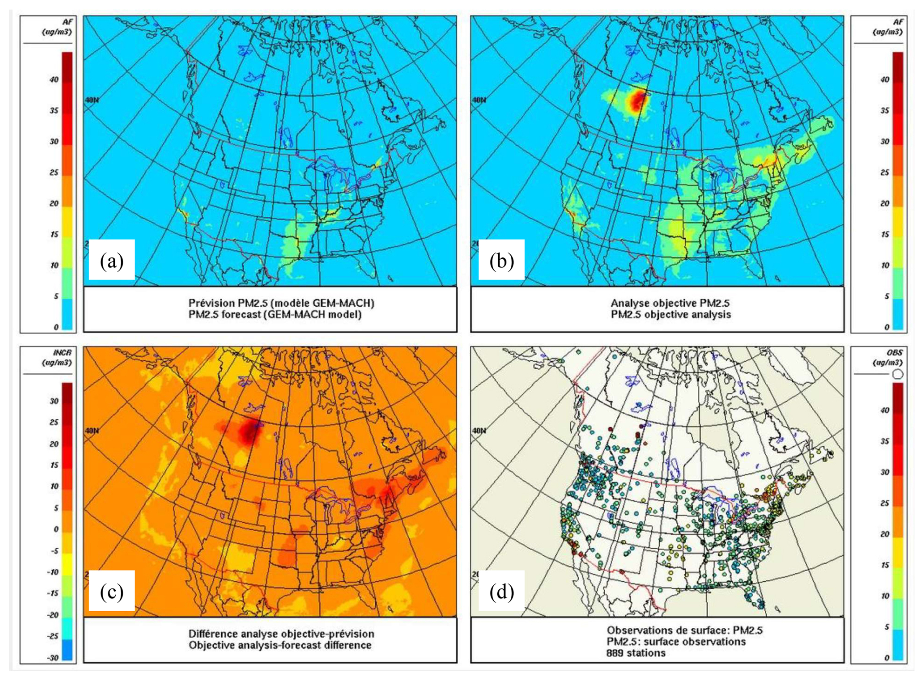
Figure 4Four-panel presentation of RDAQA 2.0.0 results for PM2.5 surface concentration (µg m−3) for 28 September 2023 at 16:00 UTC: (a) RAQDPS023 PM2.5 forecast; (b) RDAQA 2.0.0 PM2.5 objective analysis; (c) PM2.5 analysis increment (correction to the model forecast); and (d) PM2.5 surface observations.
The availability of hourly deposition flux forecast fields from the RAQDPS023 also allowed seasonal and annual dry and wet deposition fields to be accumulated on an ongoing basis. These fields could then be used to examine deposition trends and ecosystem impacts (e.g., Vet and Ro, 2008; Makar et al., 2018a, 2025). These gridded multi-month deposition fields can also be used by the ECCC ADAGIO (Atmospheric Deposition Analysis Generated by optimal Interpolation from Observations) tool, which is being developed to produce OAs of dry, wet, and total deposition of acidifying pollutants over North America (Robichaud et al., 2020) in parallel to some similar U.S. efforts (Schwede et al., 2019; Fu et al., 2022).
Wildfire smoke plume forecasts were also generated as a post-processing step. As described in Sect. 3.11.2 the RAQDPS023 served as the base platform for the ECCC RAQDPS-FW023 (“FireWork”) wildfire forecast system, which augmented the air pollutant emissions considered by the RAQDPS023 with NRT emissions from wildfires and other large BB events (Pavlovic et al., 2016; Munoz-Alpizar et al., 2017; Chen et al., 2019a; Chen and Menelaou, 2021). Both RAQDPS023 versions were run twice daily at 00:00 and 12:00 UTC for 72 h periods. Hourly forecasts of the transport and evolution of wildfire smoke plumes were then calculated as the difference between the RAQDPS-FW023 and RAQDPS023 PM2.5 forecast fields. Four post-processing products for wildfire smoke plumes were prepared and posted to an ECCC public website (https://weather.gc.ca/firework/index_e.html, last access: 18 March 2026): (i) 72 h animations of hourly ground-level smoke concentration fields (µg m−3); (ii) 72 h animations of hourly, vertically-integrated total column smoke fields (kg m−2) (this product was discontinued on 11 June 2024); (iii) 24 h mean ground-level smoke concentration fields for Days 1, 2, and 3; and (iv) 24 h maximum ground-level smoke concentration fields for Days 1, 2, and 3. Figure 5 shows examples of two of these products. RAQDPS-FW023 forecasts were also made available on the WMO North American Regional Vegetation Fire and Smoke Pollution Warning and Advisory Centre (RVFSP-WAC) website, which is operated by ECCC (https://hpfx.collab.science.gc.ca/~svfs000/na-vfsp-was/public/dist/home/introduction, last access: 18 March 2026).
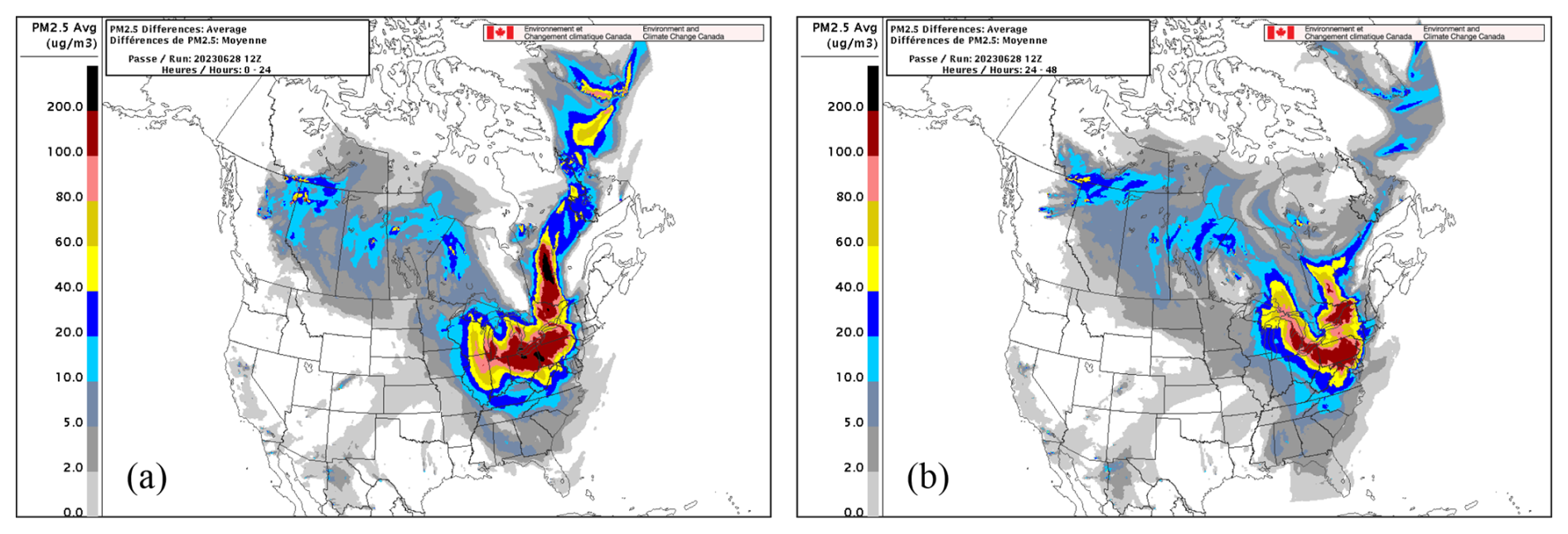
Figure 5RAQDPS-FW023 12:00 UTC forecast on 28 June 2023 of contribution of smoke from wildfires to mean surface PM2.5 concentrations (µg m−3) for hours (a) 00:00–24:00 and (b) 24:00–48:00.
5.3 Performance evaluation
The operational performance of the RAQDPS023 was routinely monitored and reported internally (e.g., Moran et al., 2021a), but only the small number of pollutants whose NRT measurements were routinely available from surface networks could be considered. These pollutants include the three AQHI component pollutants, NO2, O3, and PM2.5 total mass, plus NO, SO2, and PM10 total mass. These same six pollutants were considered by the RDAQA 2.0.0 system described above. Note that performance evaluation statistics are usually based on point measurements, but analysis increments from the RDAQA 2.0.0 can be viewed as regional errors (e.g., Fig. 4). The companion paper by Moran et al. (2026) has examined RAQDPS023 performance for five years: the first year of RAQDPS023 operational forecasts and four years of retrospective annual simulations for the 2013–2016 period. For the 2021/22 forecasts of NO2, O3, and PM2.5 total mass made by the RAQDPS023, the seasonal and annual evaluation scores for O3 hourly forecasts were generally the highest, followed by NO2 scores and then PM2.5 scores. Another important finding was that predicted monthly mean PM2.5 total mass was biased low in all months in 2021/22.
Other pollutants are also monitored, but these measurements are only available after a lag of months or even years to allow time for laboratory analysis and quality assurance/quality control (QAQC) measures and hence can only be used for retrospective performance evaluations. The companion paper by Moran et al. (2026) also examined RAQDPS023 performance using this larger suite of species measurements, including other gas-phase species, PM2.5 chemical components, and concentrations in precipitation, for the 2013–2016 retrospective simulations, which used year-specific anthropogenic emissions in place of the SET4.0.0 emissions set. Access to the much more comprehensive measurement data set provided additional insights into model performance. One insight was that one PM2.5 chemical component (SU) was consistently underpredicted for the four years while two others (EC, SS) were consistently overpredicted. O3 predictions in the spring were also biased low while isoprene predictions were biased high. These findings all suggest possible directions for model improvement. For more details see the companion paper by Moran et al. (2026).
ECCC has also been working with other agencies since 2017 to exchange, evaluate, and compare operational AQ forecasts for North America. ECCC has built an automated verification system to receive, ingest and compare these daily forecasts against surface measurements (Pavlovic et al., 2018; Moran et al., 2020b). Three regional AQ forecast models and three global AQ forecast models from five agencies are currently participating in this initiative. A performance evaluation report containing North American monthly evaluation statistics for these six models is produced every quarter by ECCC and is then made available through the WMO Global Air Quality Forecasting and Information System (GAFIS) initiative website (https://community.wmo.int/en/activity-areas/gaw/science-for-services/gafis, last access: 18 March 2026) on webpage https://hpfx.collab.science.gc.ca/~svfs000/na-aq-mm-fe/dist/ (last access: 18 March 2026). This effort is discussed in more detail in Moran et al. (2026).
The previous sections have described the RAQDPS023 and RAQDPS-FW023 operational AQ forecast systems that became operational on 1 December 2021 (Table A1). Moran et al. (2026), the companion paper to this paper, documents both strengths and weaknesses of these two systems, including some model weaknesses that future system versions might address. During the preparation of these two papers, however, a major new version of the RAQDPS, RAQDPS025, which does at least partially address some of these weaknesses, including PM2.5 total mass underpredictions, was implemented operationally on 11 June 2024 (Table A1). This section briefly summarizes the main updates and innovations introduced in the RAQDPS025 and then outlines some possible improvements for future system versions.
6.1 RAQDPS025 updates and innovations
The RAQPS025 system is documented in CMC-RAQPS025 (2024). As described below it includes two innovations related to meteorology, eight innovations related to chemistry, and one innovation related to input emissions. So-called “unit” tests were performed during the development of this new version to quantify the impact of each innovation, similar to the approach described by Foley et al. (2010). Five of these innovations were judged to have a “high” impact, five were judged to have a “medium” impact, and one was judged to have a “low” impact (CMC-RAQPS025, 2024).
The key acceptance criterion for the adoption of a new operational forecast system at ECCC is that it should improve, or at least not degrade, overall system performance regardless of whether the proposed system is believed to deliver improvements to science representations or numerical schemes or system architecture. An ECCC internal management committee is responsible for approving parallel and operational implementations of new forecast system versions. If preliminary approval is given by the committee based on evaluation results from several retrospective evaluation periods, the new forecast system is run side-by-side (i.e., in parallel) with the existing forecast system for a minimum of two months before results of evaluations for the parallel period are presented to the committee and final approval for implementation is either given or withheld. The RAQDPS025 was run in parallel with the RAQDPS024 from 13 February to 10 June 2024.
6.1.1 Updates to GEM and GEM-MACH computer codes
The RAQDPS023 was based on the GEM 5.1.0 and GEM-MACH v3.1.0.0 computer codes, and the RAQDPS024 was based on the GEM 5.1.2 and GEM-MACH v3.1.1.2 computer codes. The RAQDPS025 is based on the GEM 5.2.1 and GEM-MACH v3.2.1.1 computer codes (Table A1). Many of the following innovations were introduced with GEM-MACH v3.2.1.1.
6.1.2 Updates to meteorological piloting model
One ongoing challenge for operational forecasting at the Canadian Meteorological Centre (CMC) is providing the computer and human resources required (i) to maintain the large number of complex weather and environmental forecast systems that are being run operationally and (ii) to implement a suite of system updates at regular intervals while addressing the complicated interdependencies of these systems. As noted in Sect. 2 the regional 10 km RAQDPS023 was dependent on both the global 15 km GDPS 8.0.0 and the regional 10 km RDPS 8.0.0. In June 2024 a new version of the GDPS, GDPS 9.0.0, with horizontal grid spacing reduced to 10 km was implemented operationally, and at the same time the RDPS 8.0.0 was retired as an independent forecast system without a replacement (CMC-RDPS-9.0.0, 2024). As a consequence it was necessary to replace the RDPS 8.0.0 as the meteorological piloting model for the RAQDPS025 with the GDPS 9.0.0, but there was no loss of horizontal resolution. In principle this change also has the added benefit of allowing access to the GDPS 9.0.0 ozone field, which is updated by satellite data assimilation.
6.1.3 Merger of RAQDPS and RAQDPS-FW forecast systems
In order to identify and track BB smoke plumes by means of the “brute-force” method (Sect. 3.11.2) the ECCC AQ forecast system architecture required the same modelling system to be run twice at each forecast time, once with BB emissions (RAQDPS-FW023) and once without BB emissions (RAQDPS023). However, other approaches to track BB smoke plumes with only a single run are possible. One dynamic approach is “tagging”, in which BB emissions are tracked separately during a model simulation as “tagged” species (e.g., Wagstrom et al., 2008; Wang et al., 2009; Samaali et al., 2011; Grewe, 2013). Another approach is to include BB emissions but identify the presence of BB smoke at the post-processing stage by using known chemical characteristics of BB smoke, including both speciated PM components and gas-phase species (e.g., Akagi et al., 2011; Urbanski, 2014; Andreae, 2019; Hayden et al., 2022), to identify the locations of ambient concentrations of multiple species predicted by the model that match those chemical characteristics of BB smoke. Either approach would allow the existing system architecture to be streamlined by removing the need for two simulations with two versions of the same forecast system. However, two issues that must be considered are the different “signatures” of BB emissions associated with different ecosystems and the formation of secondary air pollutants such as O3 and SOA in BB smoke plumes in addition to the primary pollutants emitted by BB.
The second approach was adopted in the RAQDPS025 to track BB smoke plumes in a single RAQDPS025 simulation, where the ranges of two ratios of three primary PM2.5 components (EC, POM, CM) were used together to identify BB-dominated smoke plumes (CMC-RAQPS025, 2024). The lower and upper thresholds of these two ratios that identify a BB-dominated PM2.5 concentration were determined from an analysis of chemical speciation profiles of PM emissions associated with different types of wood combustion, including wildfires. This tracer-ratio approach does represent a change in strategy since the previous brute-force approach yielded PM2.5 concentration values due only to the contribution of BB emissions (i.e., fire-PM2.5) whereas the PM2.5 concentration values produced by the new approach also include the contributions of emissions from other emission source types. This loss of source differentiation will be less of an issue, however, when BB emissions are the dominant PM2.5 source. Note that in contrast to the RAQDPS023 and RAQDPS-FW023, the RAQDPS025 is referred to at ECCC as a unified AQ forecast system.
6.1.4 Updates to representation of vertical diffusion in the stable planetary boundary layer
The design philosophy for the development of the RAQDPS has been to employ GEM parameterizations without modification whenever possible. As noted in Sect. 3.1, however, the RAQDPS023 treated the vertical diffusion of chemical tracers in stable PBLs slightly differently than the vertical diffusion of meteorological tracers. GEM did impose two limiting values related to its turbulence parameterizations: a minimum Obukhov length (Sect. S1.3) and a maximum eddy dissipation length scale (Sect. S1.4). Many CTMs, on the other hand, also specify a minimum threshold value for the vertical eddy diffusivity of pollutant tracers (Kz) to avoid overpredictions of surface concentrations under stable conditions (e.g., McNider and Pour-Biazar, 2020), and a number of studies have examined CTM forecast sensitivity to the choice of this minimum value (e.g., Pleim, 2007; Jin et al., 2010; Makar et al., 2014; Li and Rappenglueck, 2018; Jia and Zhang, 2021; Jiang et al., 2024). The RAQDPS023 employed a minimum Kz value of 0.1 m2 s−1. Another CTM, the CMAQ (Community Multiscale Air Quality) model extends this approach by considering land-surface-type-dependent minimum vertical eddy diffusivity values, which are specified to be higher over urban areas (Li and Rappenglueck, 2018). This approach is appealing since urban areas have large surface roughness values and are typically also areas of high surface emissions in which surface concentrations are very sensitive to the exact balance between near-ground turbulent vertical mixing and surface emissions (Makar et al., 2014; Li and Rappenglueck, 2018). However, the specification of the allowable range of minimum eddy diffusivity values in the CMAQ scheme is still arbitrary.
Makar et al. (2021) tested a novel vertical diffusion parameterization in which the near-surface vertical diffusion of on-road vehicle emissions is modulated by vehicle-induced turbulence (VIT), which is calculated from traffic density and vehicle speeds. Like the CMAQ scheme this VIT scheme can increase vertical mixing in urban areas for stable conditions, but it also offers a physical basis for this increase and it will affect non-urban areas with high levels of traffic as well (e.g., rural highways). The VIT scheme has been implemented in the RAQDPS025. As might be expected it has a greater impact in the winter months when stable conditions are more common. A co-benefit of adding this new scheme was the elimination of the arbitrary lower limit on PBL height of 100 m and the imposed injection of area emissions into the two lowest model layers instead of the first layer alone that was used in the RAQDPS023 (Sect. 3.1).
6.1.5 Updates to chemical lateral boundary conditions
CLBCs are important for regional AQ models and may even be controlling for those species whose lifetimes are greater than a few days, which is often the time needed for an air parcel to traverse a regional model domain (e.g., Brost, 1988). Among these longer-lived species are (i) tropospheric O3, which has a lifetime of a week to several months and a globally averaged tropospheric lifetime of 22–23 d (e.g., Archibald et al., 2020), (ii) PM2.5, which has a tropospheric lifetime on the order of days to a week (e.g., Heintzenberg, 1989; Pandis et al., 1995), and (iii) CO, whose lifetime is 30–90 d (e.g., Seinfeld and Pandis, 2016). The western, northern, and eastern lateral boundaries of the RAQDPS023 continental domain are located in low-emissions regions over the Pacific Ocean, Arctic Ocean, and Atlantic Ocean, respectively, while a portion of the southern boundary is located over Mexico roughly 2500 km from the Canada-U.S. border (Fig. 2). This combination of low emissions and distance will help to reduce the contribution of CLBCs to elevated pollutant levels over Canada. On the other hand, O3 and CO have high background levels, and those levels can vary significantly with time at the lateral boundaries. For O3 those variations may be due to processes such as stratospheric O3 intrusions and trans-Pacific transport of Siberian wildfire plumes (e.g., Heald et al., 2003; Flemming et al., 2017; Pendlebury et al., 2018). PM2.5 levels can also vary with time over the oceans due to trans-oceanic transport of wildfire plumes from Siberia and desert dust from the Sahara and from northern China, Mongolia, and Central Asia (e.g., McKendry et al., 2008; Teakles et al., 2017; Tang et al., 2021).
As described in Sect. 4.2, the RAQDPS023 used “climatological” seasonal CLBCs based on results from a 2009 annual simulation with the older MOZART4 offline global CTM. For the RAQDPS025 new climatological monthly CLBC files were generated for the ADOM-2 gas-phase species by calculating monthly averages from outputs for the 2012-2019 period extracted from a 20-year global simulation made with version 6 of the Community Atmosphere Model with chemistry (CAM-chem) (Emmons et al., 2020; Tilmes et al., 2022; CMC-RAQPS025, 2024). Year-specific anthropogenic emissions for these annual simulations were obtained from CAMS-GLOB-ANT v5.1, a recent multi-year global emissions inventory (Soulie et al., 2023, 2024), and natural emissions from biogenic, biomass burning, marine, lightning, dust, and volcanic sources were also considered (Emmons et al., 2020).
While such climatological CLBCs do not address the episodic nature of the large-scale distributions of longer-lived pollutants such as O3, CO, and PM2.5, they can still be broadly representative of typical chemical inflows. The alternative is to supply time- and space-varying CLBCs based on forecasts from a compatible global chemical weather model. Such a system is currently under development at ECCC, but it is not yet ready for operational deployment.
6.1.6 Updates to representation of below-cloud scavenging of size-resolved PM
As described in Sect. 3.10 the treatment of below-cloud scavenging of PM in the RAQDPS023 was based on Slinn (1984). More recent studies by Wang et al. (2014a, b) have proposed an updated and unified parameterization of below-cloud wet removal of size-resolved PM by different precipitation types in all seasons. This newer parameterization was tested in a research version of GEM-MACH (Ghahreman et al., 2024) and was then implemented operationally in the RAQDPS025.
As well the RAQDPS023 used a fixed threshold temperature of 0 °C to define the transition between liquid cloud droplet scavenging and solid snow scavenging. In the RAQDPS025 the phase state for cloud droplets predicted by GEM cloud physics, which includes mixed-phase as well as liquid and solid hydrometeors, has been used instead (Ghahreman et al., 2024). This better aligns the treatment of below-cloud scavenging of pollutants in GEM-MACH with the treatment of cloud processes in GEM.
6.1.7 Updates to representation of gas-phase dry deposition
Three minor updates were implemented to the gas-phase dry deposition code in the RAQDPS025 (CMC-RAQPS025, 2024): (i) a correction was made to the value of the Schmidt number (changed from 0.84 to 0.62); (ii) the algorithm for calculating the ratio of the molecular diffusion coefficient for water vapour to that of a depositing pollutant species was updated; and (iii) a correction was made to the calculation of aerodynamic resistance Ra. In addition, the monthly climatology of satellite-derived, gridded LAI described by Zhang et al. (2021), which provides high-resolution (500 m), latitude-longitude-dependent descriptions of variations in this important vegetation phenological attribute, was adopted in the calculation of the surface resistance term Rc. Note that the use of monthly LAI fields reduces but does not remove the dependence on five phenological seasons that was described in Sect. 3.9.
6.1.8 Inclusion of sea salt mass in PM2.5 total dry mass calculation
As noted in Sect. 5.1 the RAQDPS023 calculated PM2.5 total mass as the sum of seven chemical components (SU, NI, AM, EC, POM, SOM, CM). This quantity corresponds to dry PM2.5 total mass (i.e., without aerosol water) without a contribution from sea salt. The SS contribution had been excluded in earlier versions of the RAQDPS due to large overpredictions that had been observed early in the development of GEM-MACH. However, corrections had been made more recently to the SS emissions scheme (Sect. 3.11.3), and performance evaluation results presented in the companion paper by Moran et al. (2026) showed that the exclusion of both SS and aerosol water contributed to the consistent RAQDPS023 underprediction of PM2.5 total mass. Sea salt was thus included in the calculation of forecast PM2.5 total mass in RAQDPS025, although Moran et al. (2026) showed that a positive bias for SS was still present.
6.1.9 Updates to solver for gas-phase chemistry
As described in Sect. 3.4 and 3.5 both the gas-phase and aqueous-phase chemistry mechanisms in the RAQDPS023 were solved for a model chemistry time step using the computationally efficient Young and Boris (1977) predictor–corrector algorithm and employing a number of smaller integration time substeps. However, the computer code used in GEM-MACH for this solver was hardcoded, was challenging to modify and maintain, and was less accurate than some other ordinary-differential-equation (ODE) solvers now available, in particular during the day-to-night and night-to-day transitions. The publicly available Kinetic PreProcessor (KPP) software tool is a symbolic preprocessor that allows chemical mechanisms to be described in a natural and compact way (cf. Table 4), permits the user to choose from a number of different ODE solvers, and then generates computer code in three high-level computer languages (Fortran, C, Matlab) (Damian et al., 2002; Sandu and Sander, 2006). As a consequence, KPP can deliver more accurate time integrations of chemistry mechanisms, and it also reduces the effort needed to modify and maintain existing chemistry mechanisms and to implement new chemistry mechanisms.
Source code generated by the KPP to use a Rosenbrock solver was introduced in the RAQDPS025 in the gas-phase chemistry operator in place of the Young-Boris solver. One additional benefit was removal of the need to make the steady-state assumption for short-lived chemical species, which can break down in the upper troposphere due to cold temperatures.
6.1.10 Updates to representation of biogenic emissions
The representation of biogenic emissions used in the RAQDPS023 (Sect. 3.11.3) was quite dated and had an overly simple treatment of the spring and autumn transition seasons. Newer versions of the BEIS scheme were available that both provide more detailed VOC emission speciations and have updates to biomass and emission factors and to the treatment of canopy leaf temperature and soil NO emissions (https://www.epa.gov/air-emissions-modeling/biogenic-emission-inventory-system-beis, last access: 18 March 2026). Newer versions were also available for the BELD land use and vegetation database that is used in the calculation of biogenic emissions (Zhang and Moran, 2020), and many satellite-based data sets are now available that can provide high-resolution descriptions of temporal and spatial variations in vegetation phenology, including LAI (e.g., Zhang et al., 2021). For example, Campbell et al. (2022) have described the impact of changing from BEIS version 3.14 coupled with the BELD3 vegetation database to BEIS version 3.61 coupled with the BELD5 vegetation database on operational U.S. NAQFC system forecasts.
For the RAQDPS025 the BEIS scheme was updated from version 3.09 to version 3.7, the BELD vegetation database was updated from version 3 to version 4 (Zhang and Moran, 2020), and the satellite-derived, high-spatial resolution LAI monthly climatology described by Zhang et al. (2021) was also adopted, but the crude five-category treatment of phenological season (Sect. 3.9) was not changed. It is also worth noting that considerable uncertainty remains around the treatment of biogenic emissions in general (e.g., Hanna et al., 2005; Warneke et al., 2010; Guenther et al., 2012), so this component of the forecast system is likely to undergo further updates in the future.
6.1.11 Updates to anthropogenic emission inventories and emissions processing methods
The SET4.0.0 emission files used by the RAQDPS023 were based on a 2020 projected Canadian anthropogenic national emissions inventory and 2023 projected U.S. and Mexican anthropogenic national emissions inventories (Sect. 3.11.1). For the RAQDPS025 the SET4.0.0 emission files were replaced by a new set of input emission files called SET5.0.0. The SET5.0.0 emission files are based on the same U.S. and Mexican projected 2023 national inventories (just one year in time before the 2024 implementation of the RAQDPS025) as the SET4.0.0 emission files, but a 2023 projected Canadian national emissions inventory based on the 2019 APEI (ECCC, 2021) was used in place of the 2020 projected Canadian emissions inventory based on the 2015 APEI (ECCC, 2016). As was the case for the national inventories used for SET4.0.0 (Sect. S2), some pre-processing was also required for this new Canadian inventory before the emissions processing step (CMC-RAQDPS-025, 2024). Some improvements were also introduced to the emissions processing methods used by the SMOKE system to prepare the SET5.0.0 emissions files (Sect. S2). These included updates to 15 Canadian gridded spatial surrogates for several important emission sectors, including RWC (CMC-RAQDPS-025, 2024).
6.2 Future work
Work is already underway on the next version of the RAQDPS, including migration to a new upgrade of the ECCC HPC system. Possible future upgrades to GEM-MACH include improvements to the chemistry and dry deposition parameterizations, anthropogenic emissions and BB and other natural emissions, and chemical lateral boundary conditions, and implementation of chemical data assimilation.
Some improvements to the representation of atmospheric chemistry might include the addition of a parameterization of marine halogen chemistry, which can influence surface ozone concentrations in coastal regions (e.g., Sarwar et al., 2015; Li et al., 2019). Newer aqueous-phase chemistry schemes are available that account for the role of individual base cations and sea salt. Some of these schemes also include oxidation pathways for SOA formation in cloud droplets, such as organic acids, glyoxal, and isoprene epoxydiols (e.g., Gong et al., 2011; Marais et al., 2016; Fahey et al., 2017; Lamkaddam et al., 2021; Luu et al., 2025). Newer versions of ISORROPIA and other inorganic heterogeneous parameterization schemes are also available that treat individual base cations explicitly (e.g., Meng et al., 1995; Fountoukis and Nenes, 2007; Miller et al., 2024). A new solver for the aqueous-phase chemistry mechanism similar to the one described in Sect. 6.1.9 could also be implemented.
It was also noted in Sect. 3.9 and 3.11.3 that the parameterizations for gas-phase dry deposition and biogenic emissions used by the RAQDPS023 rely on a crude description of phenological season with low resolution of associated temporal and spatial variations. Many satellite-based data sets are now available that can provide high-resolution descriptions of temporal and spatial variations in vegetation phenology, including longitudinal and elevation variations (e.g., Zhang and Moran, 2020; Zhang et al., 2021). One such data set was adopted for use by the RAQDPS025 (Sect. 6.1.7 and 6.1.10), but further use of such data sets could be explored. In addition, two process terms for soil wetness not currently considered by the GEM-MACH gas-phase dry deposition scheme should be included (Sect. 3.9), and different treatments of some resistance terms could be adopted (e.g., Gao and Wesely, 1995; Wesely et al., 2002).
Regarding emissions updates, as noted in Sects. 3.11.1 and 6.1.11 there is an ongoing need to make use of the most recent anthropogenic emissions inventories to prepare updated model input emission files. Thus, the SET5.0.0 emission files used by the RAQDPS025, which have a nominal base year of 2023, could be replaced by a newer set of input emission files. Also, natural windblown dust emissions were not considered by the RAQDPS023 (Sect. 3.11.3); the addition of an aeolian dust emissions scheme would provide representation of a source of emissions that is currently missing. The estimation of BB emissions by CFFEPS might be improved by updates to fuel- and location-specific emission factors based upon Canada-specific field measurement campaigns, and recent literature (e.g., Hayden et al., 2022, Binte Shahid et al., 2024; Flood et al., 2025). The companion paper by Moran et al. (2026) also found from evaluation of RAQDPS023 forecasts that the scheme used by the RAQDPS023 to modulate fugitive dust emissions according to current meteorological conditions (Sect. 3.12) should be improved.
While the treatment of CLBCs was updated in the RAQDPS025 (Sect. 6.1.5), this updated treatment is still climatological or static in nature. In principle, CLBCs should be hour- and day-specific (e.g., Giordano et al., 2015; Ma et al., 2021; Tang et al., 2021). For example, Pendlebury et al. (2018) have described an approach whereby time-varying O3 CLBCs can be obtained from a monthly global O3 climatology combined with GEM model predictions of dynamic tropopause height at each time step. Another possibility to improve the CLBCs used by the RAQDPS would be to run GEM-MACH in a global configuration and then extract regional CLBCs from its forecasts (Chen et al., 2020).
Lastly, the introduction of meteorological data assimilation for the initialization of NWP models resulted in a step change in weather forecasting skill (e.g., Simmons and Hollingsworth, 2002; Bauer et al., 2015). Chemical data assimilation (CDA) offers the possibility of similar improvements for chemical weather forecasting. Some global NWP models and CTMs have implemented data assimilation of select chemical fields such as O3, CO, NO2, HCHO, PM2.5, and aerosol optical depth (AOD) to improve their initialization of the chemical state (e.g., Pierce et al., 2007; Benedetti et al., 2009; Saide et al., 2013; Inness et al., 2015, 2019; Chai et al., 2017; Randles et al., 2017; Tang et al., 2017; Kumar et al., 2019; Menut and Bessagnet, 2019; Rochon et al., 2019; CMC-GDPS-8.0.0, 2021a; Ma et al., 2021). At the same time the number of available AQ measurements for North America, especially from satellite-based sensors but also from surface-based sensors, continues to increase (e.g., Naeger et al., 2021; Jaffe et al., 2023).
An important development goal for the RAQDPS is to implement an operational CDA capability, and some options to do this are available now. These include the assimilation of surface measurements based on the RDAQA system (Sect. 5.2; Robichaud, 2017; Ménard, 2021) and the use of the assimilated O3 field from GDPS 9.0.0 forecasts (Sect. 6.1.2; Rochon et al., 2019; CMC-GDPS-8.0.0, 2021a).
Environment and Climate Change Canada (ECCC) has run an operational, continental-scale Regional Air Quality Deterministic Prediction System (RAQDPS) for North America since 2001. The earliest version of the RAQDPS employed an offline chemical transport model called CHRONOS that used the ECCC Global Environmental Multiscale (GEM) numerical weather prediction model as a meteorological driver. In 2009 CHRONOS was replaced in the RAQDPS by the online, one-way-coupled GEM-MACH (Global Environmental Multiscale–Modeling Air quality and CHemistry) chemical weather model, which consists of GEM as a meteorological host model and an embedded chemistry module named MACH (Modelling Air quality and CHemistry) that can be activated (or not) by a namelist setting. Since 2009 there have been 24 upgrades of varying magnitude made to the GEM-MACH-based version of the RAQDPS to improve forecast skill and to adjust to changes in upstream meteorological systems and ECCC's supercomputers (Table A1). This paper describes version 023 of the RAQDPS, including its dynamics, physics, chemistry, numerics, inputs, outputs, related upstream meteorological systems and downstream AQ systems, and recent and potential future developments. Significantly, it is the first comprehensive publication describing any RAQDPS version. A companion paper (Moran et al., 2026) provides a comprehensive evaluation of RAQDPS023 performance for its first forecast year and four hindcast years.
The RAQDPS023 (or RAQDPS-OP023) became the ECCC operational regional AQ forecast system on 1 December 2021; it was then migrated without any algorithmic changes to a new ECCC computer system on 28 June 2022 and renamed RAQDPS-OP024. It then continued to run operationally for another two years until it was replaced by an upgraded version, the RAQDPS025, on 11 June 2024. A special wildfire version of the RAQDPS-OP023 called FireWork023 or RAQDPS-FW023, which was identical to the RAQDPS-OP023 except for the addition of near-real-time (NRT) biomass burning (BB) emissions as an input, went operational at the same time, was migrated to the new computer system at the same time (RAQDPS-FW024), and was replaced at the same time in 2024. Running this second member of the ECCC regional AQ forecast suite allowed forecasts of the transport and diffusion of wildfire smoke plumes to be calculated in a post-processing step as the difference between the PM2.5 forecasts from the two model versions.
The RAQDPS-OP023 and RAQDPS-FW023 both used GEM-MACH version 3.1.0.0, which was built on GEM version 5.1.0. Both systems employed a regional configuration with 10 km horizontal grid spacing and a geographic domain covering Canada, the continental U.S. and most of Alaska, and northern Mexico. Both systems were run twice each day starting at 00:00 and 12:00 UTC to produce 72 h forecasts. The RAQDPS-FW023 obtained NRT satellite-detected BB emission forecasts for Canada and the U.S. for the next 72 h from version 4.1 of the Canadian Forest Fire Emissions Prediction System (CFFEPS) before each run (Sect. S3).
To obtain the meteorological initial conditions and boundary conditions that were needed, each RAQDPS023 run followed a run for the same forecast period by the corresponding ECCC operational regional weather forecast system, the 10 km Regional Deterministic Prediction System 8.0.0. The RDPS 8.0.0 was a regional configuration of GEM 5.1.0 that made 84 h forecasts four times per day. Its horizontal grid was a superset of the RAQDPS023 grid. To obtain the meteorological initial conditions and boundary conditions that it needed in turn, each RDPS 8.0.0 run followed a run for the same forecast period by the ECCC operational global weather forecast system, the 15 km Global Deterministic Prediction System 8.0.0. The GDPS 8.0.0 was a global configuration of GEM 5.1.0 that made 144 h forecasts four times per day. For maximum consistency the GDPS 8.0.0, RDPS 8.0.0, and RAQDPS023 all used the same rotated latitude-longitude map projection and the same 84 staggered hybrid vertical levels with a top at 0.1 hPa.
All three systems also employed the same GEM dynamical core, including the hydrostatic assumption. Time integration was performed using a two-time-level, iterative-implicit, three-dimensional semi-Lagrangian scheme. The GDPS 8.0.0 used a 450 s dynamics integration time step while both the RDPS 8.0.0 and RAQDPS023 used a 300 s time step. Since semi-Lagrangian advection schemes do not conserve mass, a shape-preserving monotonicity correction and a global mass fixer were both used for tracer advection for all three systems. Mass conservation is very relevant for a regional AQ model since there can be many sharp chemical concentration gradients in the vicinity of strong local emissions sources, and the resulting loss of shape preservation after advection can introduce physically unrealistic negative concentrations or positive overshoots. The same physics parameterizations were also used by the three systems (Table 1), with only very minor differences in a few parameter settings between the global and regional versions to account for their different horizontal grid spacing. And since GEM-MACH is an online model the RAQDPS023 could access many meteorological variables predicted by GEM 5.1.0 that were needed by some MACH chemistry parameterizations (Table 2).
The RAQDPS023 predicted 41 gas-phase species and 18 particle-phase chemical species, but its three key AQ predictands were NO2, O3, and PM2.5 total mass, which are needed to calculate the Canadian Air Quality Health Index. The AQHI is a health-based, multi-pollutant, additive, no-threshold hourly AQ index that is used to communicate current and predicted AQ levels to the Canadian public. Of these three predictands, PM2.5 mass poses a particular challenge because it is a complex pollutant: it has a wide size range; it is composed of many elements and compounds, both inorganic and organic; it is subject to many physical and chemical processes; and it has many types of emissions sources.
The MACH chemistry module employs a sectional representation to model the PM size distribution, where the number of size bins can be specified by the user. For the RAQDPS023 as well as earlier versions, a major simplification made to ensure that system execution times would be short enough to fit within its operational 30 min time slot was to consider just two PM size bins, one corresponding to particle Stokes diameters in the 0–2.5 µm range (“fine fraction” or PM2.5) and the other to the 2.5–10 µm range (“coarse fraction” or PMcf). Together these two size bins constitute PM10. This is a very coarse representation of the PM size distribution, but it still allowed the model to predict concentrations of PM2.5 and PM10, which are the two PM size ranges considered by most AQ measurement networks and emission inventories. MACH for the RAQDPS023 also represented PM2.5 chemical composition with a limited number of chemical components, namely sulfate, nitrate, ammonium, elemental carbon, primary organic matter, secondary organic matter, crustal material, sea salt, and aerosol water. However, these nine chemical components align fairly well with the chemical components that are measured by PM2.5 speciation networks, thus permitting evaluation of PM2.5 composition predictions. A third simplification in the treatment of PM was that each size bin was assumed to be internally mixed, an assumption that is the least good close to sources of PM but which improves as particles age in the atmosphere.
MACH contains parameterizations to represent a number of physical and chemical processes that influence PM mass concentrations. As described in Sect. 3 these include anthropogenic emissions, smokestack plume rise, sea-salt and biogenic emissions, particle nucleation, condensational growth, coagulation, gravitational settling and dry deposition, hygroscopic growth and aerosol particle activation, vertical diffusion, gas-phase chemistry, secondary organic aerosol formation, gas-particle partitioning, inorganic heterogeneous chemistry, aqueous-phase chemistry, and in-cloud and below-cloud precipitation scavenging.
Chemical tracer initial conditions for the RAQDPS023 were copies of the chemical tracer fields corresponding to that initial time from the previous forecast, a so-called perpetual forecast approach. Chemical lateral boundary conditions were obtained from a set of “climatological” seasonal vertical cross-sections of model species mass mixing ratios (MMRs) supplied for each lateral boundary. One other simplification made for the RAQDPS023 to reduce execution time was to call the MACH module every third dynamics time step, that is, to employ a chemistry time step of 900 s. This simplification was possible due to the assumption that there was no feedback of chemistry on meteorology. Even so, activation of the MACH chemistry module increased RAQDPS023 execution time by a factor of 4.4 compared to running only the GEM code.
The pre-processed, hourly, gridded anthropogenic emissions input files used by the RAQDPS-OP023 and RAQDPS-FW023, which are referred to as SET4.0.0 emissions, were new to this version (Table A1). They were based on three national emission inventories: (i) a projected 2020 Canadian Air Pollutant Emissions Inventory; (ii) a projected 2023 U.S. National Emissions Inventory (NEI); and (iii) a projected 2023 Mexican NEI. The SET4.0.0 files were generated during the development of the RAQDPS-OP023 and well before its operational deployment using version 4.7 of the SMOKE emissions processing system. Hourly BB emissions, on the other hand, were forecast for the next 72 h in advance of each RAQDPS-FW023 run by CFFEPS v4.1. Biogenic emissions were treated in a third way; they were estimated every chemistry time step by inline code in MACH. Sea-salt emissions were also estimated every chemistry time step.
The RAQDPS023 routinely output a large number of hourly gridded fields, including 41 gas-phase chemical MMR fields, eight PM2.5 and eight PMcf chemical component MMR fields, PM2.5 and PM10 total mass concentration fields, 21 dry deposition flux fields, 12 wet deposition flux fields, and four biogenic emission flux fields. Two downstream operational systems made use of some of these outputs. Point-specific hourly forecasts of NO2, O3, and PM2.5 concentrations at Canadian AQ measurement station locations were fed to the Updateable Model Output Statistics for Air Quality (UMOS-AQ) system. UMOS-AQ is a statistical post-processing package for bias correction that can compensate for systematic model errors and account for unresolved SGS phenomena. Its hourly, station-specific regression coefficients are recalculated weekly. A second post-processing system, version 2.0.0 of the Regional Deterministic Air Quality Analysis (RDAQA) system, used RAQDPS023 hourly gridded forecast fields as first-guess fields together with surface AQ measurements to generate objective analyses of hourly North American surface concentration fields for O3, NO2, NO, PM2.5, PM10, SO2, and the AQHI. RAQDPS023 forecast performance was also monitored on an ongoing basis, including by a quarterly comparison with AQ forecasts for North America made by four international operational models.
The paper concludes by describing the main innovations made for the RAQDPS025, the successor to the RAQDPS023, which was implemented operationally in June 2024. One key innovation of the RAQDPS025 was to combine the RAQDPS-OP and RAQDPS-FW systems into a single unified system while still identifying wildfire smoke plumes. The RAQDPS025 also has updates to the treatments of vertical diffusion, gas-phase chemistry, gas-phase dry deposition, below-cloud scavenging of size-resolved PM, chemical lateral boundary conditions, and biogenic emissions. As well the meteorological piloting model was changed (to GDPS 9.0.0) and a new set of anthropogenic input emissions files (SET5.0.0) was introduced. Lastly, a short summary of some possible areas of improvements to future RAQDPS versions is provided.
| ADAGIO | Atmospheric Deposition Analysis Generated by optimal Interpolation from Observations |
| ADOM | Acid Deposition and Oxidant Model |
| AGL | above ground level |
| ALKA | See Table 3 |
| ALKE | See Table 3 |
| AM | ammonium |
| AOD | aerosol optical depth |
| APEI | Air Pollutant Emissions Inventory (Canada) |
| AQ | air quality |
| AQHI | Air Quality Health Index (Canada) |
| ARCTAS | Arctic Research of the Composition of the Troposphere from Aircraft and Satellites |
| AROM | See Table 3 |
| AURAMS | A Unified Regional Air quality Modelling System |
| BB | biomass burning |
| BC | black carbon |
| BEIS | Biogenic Emission Inventory System |
| BELD3 | Biogenic Emissions Landuse Database version 3 |
| CAC | criteria air contaminant |
| CAM | Canadian Aerosol Module |
| CAM-chem | Community Atmosphere Model with chemistry |
| CAPE | convective available potential energy |
| CCN | cloud condensation nuclei |
| CDA | chemical data assimilation |
| CF | coarse fraction |
| CFC | chlorofluorocarbon |
| CFFEPS | Canadian Forest Fire Emissions Prediction System |
| CFS | Canadian Forest Service |
| CHRONOS | Canadian Hemispheric and Regional Ozone and NOx System |
| CLBC | chemical LBC |
| CM | crustal material |
| CMAQ | Community Multiscale Air Quality model |
| CMAS | Community Modeling and Analysis System (University of North Carolina) |
| CMC | Canadian Meteorological Centre |
| CS | condensable species |
| CSN | Chemical Speciation Network (U.S.) |
| CTM | chemical transport model |
| CWFIS | Canadian Wildland Fire Information System |
| DDF | dry deposition scaling factor |
| DOW | day of the week |
| EC | elemental carbon |
| ECCC | Environment and Climate Change Canada |
| EOTH | emissions of “other” VOCs (NAPAP classes 21, 23, 25, 26, 31, and 32) |
| EPA | Environmental Protection Agency (U.S.) |
| FBP | (Canadian) Forest Fire Behaviour Prediction subsystem |
| FEPS | Fire Emission Production Simulator (U.S.) |
| FW | FireWork |
| FWI | (Canadian) Forest Fire Weather Index subsystem |
| GAFIS | Global Air quality Forecasting and Information System initiative (WMO) |
| GDPS | Global Deterministic Prediction System |
| GEM | Global Environmental Multiscale (model) |
| GEM-MACH | Global Environmental Multiscale–Modelling Air quality and CHemistry (model) |
| GMM | gram molar mass |
| HETV | HETerogeneous Vectorized scheme |
| HPC | high-performance computing |
| IAU | incremental analysis update |
| IAY | instantaneous aerosol yield |
| IC | initial condition |
| ILMC | iterative locally mass conserving (scheme) |
| IMPROVE | Interagency Monitoring of Protected Visual Environments network (U.S.) |
| ISBA | Interactions between Soil–Biosphere–Atmosphere (land surface model) |
| ISOP | isoprene (see Table 3) |
| ISORROPIA | “equilibrium” (modern Greek) |
| KPP | Kinetic PreProcessor |
| LAI | leaf area index |
| LAM | limited area model |
| LBC | lateral boundary condition |
| LINOZ | LINearized OZone mechanism |
| LST | local standard time |
| LWC | liquid water content |
| MACH | Modelling Air quality and CHemistry (module) |
| MLR | multi-variate linear regression |
| MMR | mass mixing ratio |
| MODIS | Moderate Resolution Imaging Spectroradiometer |
| MOS | model output statistics |
| MOZART4 | Model for OZone And Related chemical Tracers version 4 |
| MPI | Message Passing Interface |
| NAPAP | National Acid Precipitation Assessment Program (U.S.) |
| NAPS | National Air Pollution Surveillance system (Canada) |
| NAQFC | National Air Quality Forecast Capability (U.S.) |
| NASA | National Aeronautics and Space Administration (U.S.) |
| NEI | National Emissions Inventory (U.S., Mexico) |
| NI | nitrate |
| NMHC | non-methane hydrocarbon |
| NOAA | National Oceanic and Atmospheric Administration (U.S.) |
| NRT | near-real time |
| NWP | numerical weather prediction |
| OA | objective analysis |
| ODE | ordinary differential equation |
| OH | hydroxl radical |
| OI | optimal interpolation |
| OpenMP | Open Multi-Processing |
| OVOC | other VOCs |
| PAR | photosynthetic active radiation |
| PBL | planetary boundary layer |
| PM | particulate matter |
| PMcf | PM coarse fraction (2.5–10 µm) |
| PM2.5 | PM with aerodynamic diameter of less than 2.5 µm |
| PM10 | PM with aerodynamic diameter of less than 10 µm |
| POM | primary organic matter |
| QA/QC | quality assurance/quality control |
| RAQDPS | Regional Air Quality Deterministic Prediction System |
| RAQDPS-FW | Operational RAQDPS with FireWork BB emissions |
| RAQDPS-OP | Operational RAQDPS without FireWork BB emissions |
| RDAQA | Regional Deterministic Air Quality Analysis |
| RDPS | Regional Deterministic Prediction System |
| RH | relative humidity |
| ROS | rate of spread |
| RVFSP-WAC | North American Regional Vegetation Fire and Smoke Pollution Warning and Advisory Centre |
| RWC | residential wood combustion |
| SCC | source classification code |
| SGS | subgrid-scale |
| SI | Système International d'unités |
| SMOKE | Sparse Matrix Operation Kernel Estimation system (CMAS) |
| SOA | secondary organic aerosol |
| SOM | secondary organic matter |
| SS | sea salt |
| SU | sulfate |
| TF | transportable fraction |
| TKE | turbulent kinetic energy |
| TOLU | See Table 3 |
| UMOS-AQ | Updateable Model Output Statistics–Air Quality |
| USFS | U.S. Forest Service |
| UTC | Universal Time Coordinated |
| VIIRS | Visible Infrared Imaging Radiometer Suite |
| VIT | vehicle-induced turbulence |
| VOC | volatile organic compound |
| WA | aerosol water |
| WHO | World Health Agency |
| WMO | World Meteorological Organization |
| 4D-IAU | four-dimensional incremental analysis update |
List of symbols
| d | particle diameter (cm) |
| D | raindrop or frozen hydrometeor diameter (cm) |
| Di | gas-phase diffusivity of species i (cm2 s−1) |
| Dm | mean raindrop or frozen hydrometeor diameter (cm) |
| mean snowflake-particle collection efficiency (unitless) | |
| E(d,Dm) | raindrop-particle collection efficiency (unitless) |
| mean raindrop-particle collection efficiency (unitless) | |
| fcld | total cloud cover fraction by layer (unitless) |
| fctr | precipitation production rate (s−1) |
| H′ | effective equilibrium constant for gas-liquid partitioning |
| K | equilibrium constant for aqueous-phase reactions |
| Kom,1i | first partitioning coefficient of the ith condensable species (µg m−3) |
| Kom,2i | second partitioning coefficient of the ith condensable species (µg m−3) |
| Kz | vertical eddy diffusivity for tracers (m2 s−1) |
| L | characteristic collection length scale of frozen hydrometeor (may not be D) (cm) |
| L | liter |
| Lw | volumetric liquid water fraction in air (m3 H2O per m3 air) |
| N | number of size bins or sections |
| Nd | cloud droplet number concentration (cm−3) |
| Np | particle number density (cm−3) |
| Np,i | particle number density in size bin i (cm−3) |
| P | (liquid) precipitation rate (mm h−1) |
| P | atmospheric pressure (hPa) |
| ps | surface pressure (hPa) |
| R | universal gas constant (J K−1 mol−1 or L atm K−1 mol−1) |
| Ra | aerodynamic resistance (s m−1) |
| Rb | quasi-laminar sublayer resistance (s m−1) |
| Rc | surface resistance (s m−1) |
| Ri | gradient Richardson number (unitless) |
| Rib | bulk Richardson number (unitless) |
| T | dry-bulb temperature (K) |
| u∗ | friction velocity (m s−1) |
| Vrt | raindrop terminal fall speed (m s−1) |
| Vst | frozen hydrometeor terminal fall speed (m s−1) |
| α1i | mass-based stoichiometric coefficient 1 for SOA formation from ith CS (unitless) |
| α2i | mass-based stoichiometric coefficient 2 for SOA formation from ith CS (unitless) |
| λ | turbulence-regime-specific mixing length (m) |
| λe | dissipation length scale (m) |
| Λr(d) | rain scavenging rate coefficient for aerosol particles of diameter d (s−1) |
| Λs(d) | snow scavenging rate coefficient for aerosol particles of diameter d (s−1) |
| Λi | rain scavenging rate coefficient for ith gas (s−1) |
Table A1Chronology of operational RAQDPS and RAQDPS-FW versions. Boldface font indicates a major update to the RAQDPS version and the RAQDPS-FW version (which was introduced operationally in April 2016 as a seasonal forecast system). (See also ECCC changelogs for the RAQDPS (https://eccc-msc.github.io/open-data/msc-data/nwp_raqdps/changelog_raqdps_en/, last access: 18 March 2026) and RAQDPS-FW (https://eccc-msc.github.io/open-data/msc-data/nwp_raqdps-fw/changelog_raqdps-fw_en/, last access: 18 March 2026).)
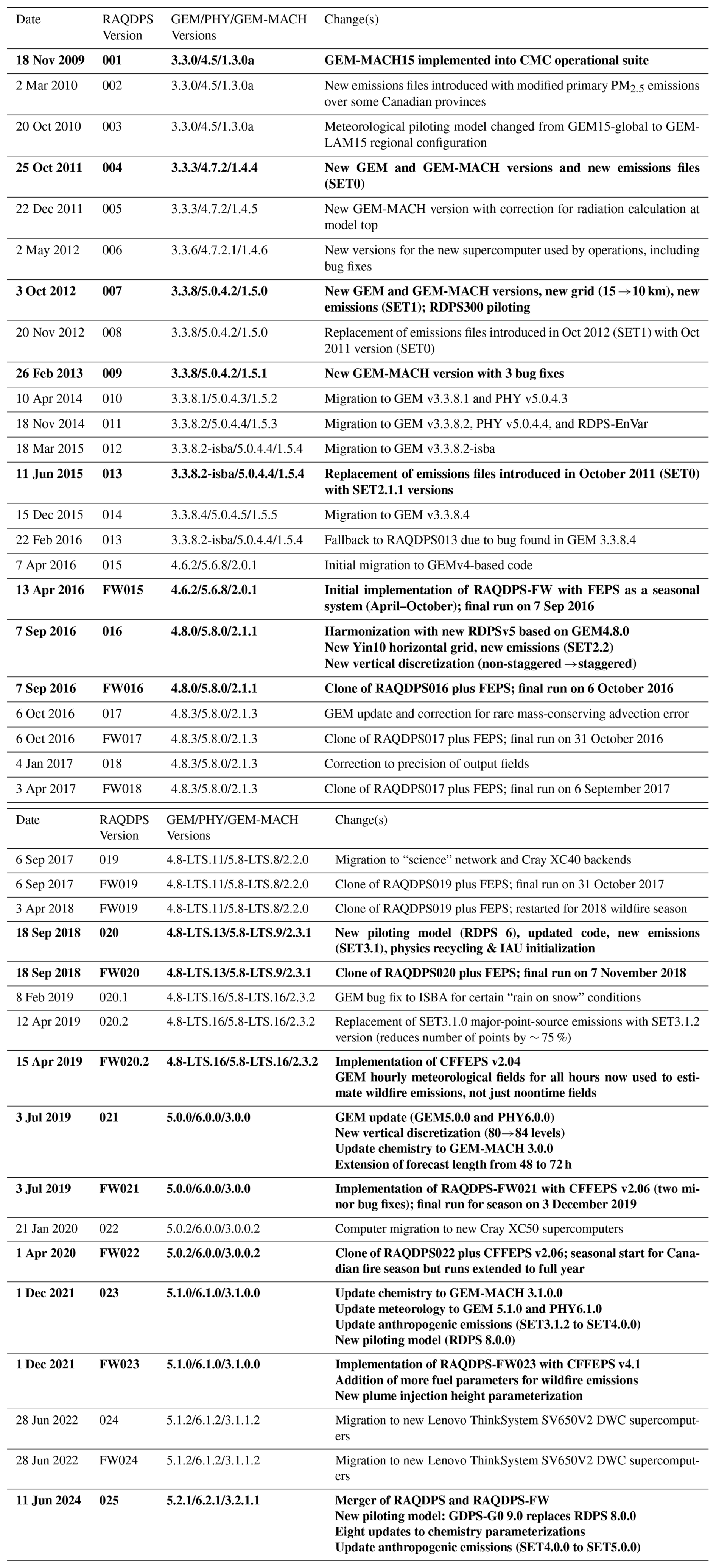
Version 5.1 of the GEM numerical weather prediction model code used by the RAQDPS023 is free software which can be redistributed and/or modified under the terms of version 2.1 of the GNU Lesser General Public License as published by the Free Software Foundation. The GEM source code has been developed by the Meteorological Research Division of ECCC. This code is available for download from https://doi.org/10.5281/zenodo.17782580 (Environment and Climate Change Canada, 2025).
MACH, the atmospheric chemistry library for the GEM numerical atmospheric model (© 2007–2021, Air Quality Research Division and National Prediction Operations Division, Environment and Climate Change Canada) is free software that can be redistributed and/or modified under the terms of the GNU Lesser General Public License as published by the Free Software Foundation – either version 2.1 of the license or any later version. The GEM-MACH version 3.1.0.0 code used by the RAQDPS023 can be downloaded from website https://doi.org/10.5281/zenodo.15330612 (Savic-Jovcic et al., 2025). Related documentation is also available on that website, including information about key input and configuration files and copies of several reports referenced in this paper. The GEM-MACH v3.1.1.2 source code for the RAQDPS024, an equivalent version to the RAQDPS023 that went into operation after a migration to a new ECCC high-performance computer system in June 2022, is available at https://doi.org/10.5281/zenodo.13952893 (GEM-MACH development team, 2022).
The CFFEPS version 4.1 code was used by the RAQDPS-FW023 and RAQDPS-FW024. It is free software that can be redistributed and/or modified under the terms of the GNU Lesser General Public License, either version 2.1 or any later version, as published by the Free Software Foundation. It is available to download from website https://doi.org/10.5281/zenodo.15305591 (Anderson and Chen, 2021).
The supplement related to this article is available online at https://doi.org/10.5194/gmd-19-4137-2026-supplement.
MDM was the science lead for the development of the RAQDPS from the RAQDPS001 up to RAQDPS023 and co-supervisor of all operational deliveries over that period. He conceived and prepared the original and final drafts of this paper. VSJ was the RAQDPS code librarian, lead tester for RAQDPS development, and contributed to the original and final draft of the manuscript. CAS was the science lead for the development and co-supervisor for the operational deliveries of RAQDPS024 and RAQDPS025. SM was co-supervisor of many operational deliveries of the RAQDPS with assistance from KM and RMA on testing and evaluation. WG, CAS, SM, AA, VSJ, and MDM contributed to the development of different versions of the GEM-MACH code. JZ and QZ were responsible for emissions processing and the preparation of the SET4.0.0 emission input files and contributed to Table 9. JC and AA worked on RAQDPS-FW and CFFEPS development. AL focused on model performance evaluation and contributed to the original draft of the manuscript. Lastly, VSJ, CAS, WG, JZ, JC, SM, RMA, QZ, and AL reviewed the manuscript.
The contact author has declared that none of the authors has any competing interests.
Publisher's note: Copernicus Publications remains neutral with regard to jurisdictional claims made in the text, published maps, institutional affiliations, or any other geographical representation in this paper. The authors bear the ultimate responsibility for providing appropriate place names. Views expressed in the text are those of the authors and do not necessarily reflect the views of the publisher.
The authors are deeply indebted to many colleagues in the Meteorological Research Branch and the Canadian Meteorological Centre of ECCC for their work over many years on the development and operational implementation of the GEM numerical weather prediction model. We would like to thank the many people who contributed in some way to the development, evaluation, and implementation of various versions of the RAQDPS and its downstream systems. They include the following current or former ECCC colleagues: David Anselmo, Stavros Antonopoulos, Paul-André Beaulieu, Véronique Bouchet, Elisa Boutzis, Stéphane Chamberland, Shawn Corvec, Sophie Cousineau, Louis-Philippe Crevier, Didier Davignon, Jean de Grandpré, Annie Duhamel, Amin Erfani, Nicolas Gasset, Samuel Gilbert, Sunling Gong, Ping Huang, Irena Ivanova, Alexander Kallaur, Setigui Keita, Dragana Kornic, Hugo Landry, Patrick Manseau, Ron McTaggart-Cowan, Richard Ménard, Thomas Milewski, Richard Moffet, Jacques Montpetit, Heather Morrison, David Niemi, Balbir Pabla, Alain Patoine, Radenko Pavlovic, Diane Pendlebury, Si-Jun Peng, Alain Robichaud, Jacinthe Racine, Matt Reszka, Mourad Sassi, Leo Separovic, Donald Talbot, Kenjiro Toyota, Ayrton Zadra, and Yulia Zaitseva. Many thanks are also due to Kerry Anderson, Peter Englefield, and Dan Thompson of the Canadian Forest Service for their help with the CWFIS and CFFEPS, to Susan O'Neill and Tara Strand of the U.S. Forest Service for their assistance with FEPS, and to Sarah Henderson of the University of British Columbia for collaborating on FireWork analysis. Jérôme Alary, Marc Deslauriers, Francois Lavallée, Anne Monette, Steve Smyth, Brett Taylor, and Shawn Tobin of the ECCC Science Reporting and Assessment Directorate helped us in many ways with accessing, preparing, and processing modelling versions of multiple Canadian national emissions inventories. We very much appreciate the considerable help with modelling versions of various U.S. national emission inventories that we have received over many years from Alison Eyth and George Pouliot of the U.S. EPA. We also acknowledge our continuing access to NRT surface AQ measurements provided by Canada's National Air Pollutant Surveillance network and its provincial, territorial, and regional government partners and by the U.S. EPA AIRNow metanetwork and its state and local, tribal, federal, Canadian, and Mexican partners and to MODIS and VIIRS imagery provided by NOAA and NASA. MDM would also like to thank Paul Makar of ECCC for his many contributions to the development of GEM-MACH, Sylvie Gravel, now retired from ECCC, for her many contributions to the development of GEM-MACH and for reviewing the manuscript, Ron McTaggart-Cowan of ECCC for reviewing the manuscript, and Rosa Wu of ECCC for her unstinting support of this project over multiple years. Lastly, the authors would like to acknowledge two anonymous reviewers for their constructive and insightful comments that helped to improve the manuscript, and the topic editor, Emmanouil Flaounas, for overseeing the review of two lengthy manuscripts.
This paper was edited by Emmanouil Flaounas and reviewed by two anonymous referees.
Akagi, S. K., Yokelson, R. J., Wiedinmyer, C., Alvarado, M. J., Reid, J. S., Karl, T., Crounse, J. D., and Wennberg, P. O.: Emission factors for open and domestic biomass burning for use in atmospheric models, Atmos. Chem. Phys., 11, 4039–4072, https://doi.org/10.5194/acp-11-4039-2011, 2011.
Akingunola, A., Makar, P. A., Zhang, J., Darlington, A., Li, S.-M., Gordon, M., Moran, M. D., and Zheng, Q.: A chemical transport model study of plume-rise and particle size distribution for the Athabasca oil sands, Atmos. Chem. Phys., 18, 8667–8688, https://doi.org/10.5194/acp-18-8667-2018, 2018.
Anderson, G. K., Sandberg, D. V., and Norhelm, R. A.: Fire Emission Production Simulator (FEPS) User's Guide Version 1., Pacific Northwest Research Station, U.S. Forest Service, Portland, Oregon, January, 97 pp., https://share.google/yCxzmeNyLzeDFR5Zf (last access: 30 March 2026), 2004.
Anderson, K. and Chen, J.: Canadian Fire Emissions Prediction System (CFFEPS) v4.1, Zenodo [code], https://doi.org/10.5281/zenodo.15305591, 2021.
Andreae, M. O.: Emission of trace gases and aerosols from biomass burning – an updated assessment, Atmos. Chem. Phys., 19, 8523–8546, https://doi.org/10.5194/acp-19-8523-2019, 2019.
Ansari, A. S. and Pandis, S. N.: Response of inorganic PM to precursor concentrations, Environ. Sci. Technol., 32, 2706–2714, https://doi.org/10.1021/es971130j, 1998.
Anselmo, D., Moran, M. D., Ménard, S., Bouchet, V., Makar, P., Gong, W., Kallaur, A., Beaulieu, P.-A., Landry, H., Stroud, C., Huang, P., Gong, S., and Talbot, D.: A new Canadian air quality forecast model: GEM-MACH15, in: Proc. 12th AMS Conf. on Atmos. Chem., 17–21 January, Atlanta, Georgia, 6 pp., https://ams.confex.com/ams/pdfpapers/165388.pdf (last access: 30 March 2026), 2010.
Antonopoulos, S., Bourgouin, P., Montpetit, J., and Croteau, G.: Forecasting O3, PM2.5 and NO2 hourly spot concentrations using an updatable MOS methodology, in: Air Pollution Modeling and its Application XXI, edited by: Steyn, D. G. and Trini Castelli, S., Springer Netherlands, Dordrecht, 309–314, https://doi.org/10.1007/978-94-007-1359-8_53, 2011.
Appel, K. W., Foley, K. M., Bash, J. O., Pinder, R. W., Dennis, R. L., Allen, D. J., and Pickering, K.: A multi-resolution assessment of the Community Multiscale Air Quality (CMAQ) model v4.7 wet deposition estimates for 2002–2006, Geosci. Model Dev., 4, 357–371, https://doi.org/10.5194/gmd-4-357-2011, 2011.
Aranami, K., Davies, T., and Wood, N.: A mass restoration scheme for limited-area models with semi-Lagrangian advection, Q. J. Roy. Meteor. Soc., 141, 1795–1803, https://doi.org/10.1002/qj.2482, 2015.
Archibald, A. T., Neu, J. L., Elshorbany, Y. F., Cooper, O. R., Young, P. J., Akiyoshi, H., Cox, R. A., Coyle, M., Derwent, R. G., Deushi, M., Finco, A., Frost, G. J., Galbally, I. E., Gerosa, G., Granier, C., Griffiths, P. T., Hossaini, R., Hu, L., Jöckel, P., Josse, B., Lin, M. Y., Mertens, M., Morgenstern, O., Naja, M., Naik, V., Oltmans, S., Plummer, D. A., Revell, L. E., Saiz-Lopez, A., Saxena, P., Shin, Y. M., Shahid, I., Shallcross, D., Tilmes, S., Trickl, T., Wallington, T. J., Wang, T., Worden, H. M., and Zeng, G.: Tropospheric Ozone Assessment Report: A critical review of changes in the tropospheric ozone burden and budget from 1850 to 2100, Elem. Sci. Anthr., 8, 034, https://doi.org/10.1525/elementa.2020.034, 2020.
Atkinson, R.: Gas-phase tropospheric chemistry of organic compounds: A review, Atmos. Environ., 24, 1–41, https://doi.org/10.1016/0960-1686(90)90438-S, 1990.
Atkinson, R., Baulch, D. L., Cox, R. A., Hampson, R. F., Kerr, J. A., and Troe, J.: Evaluated kinetic and photochemical data for atmospheric chemistry: Supplement IV. IUPAC subcommittee on gas kinetic data evaluation for atmospheric chemistry, J. Phys. Chem. Ref. Data, 21, 1125–1568, https://doi.org/10.1063/1.555918, 1992.
Ault, A. P., Moffet, R. C., Baltrusaitis, J., Collins, D. B., Ruppel, M. J., Cuadra-Rodriguez, L. A., Zhao, D., Guasco, T. L., Ebben, C. J., Geiger, F. M., Bertram, T. H., Prather, K. A., and Grassian, V. H.: Size-dependent changes in sea spray aerosol composition and properties with different seawater conditions, Environ. Sci. Technol., 47, 5603–5612, https://doi.org/10.1021/es400416g, 2013.
Baklanov, A. and Zhang, Y.: Advances in air quality modeling and forecasting, Glob. Transit., 2, 261–270, https://doi.org/10.1016/j.glt.2020.11.001, 2020.
Barrie, L. A. and Georgii, H. W.: An experimental investigation of the absorption of sulphur dioxide by water drops containing heavy metal ions, Atmos. Environ. 1967, 10, 743–749, https://doi.org/10.1016/0004-6981(76)90075-5, 1976.
Barrie, L. A., Yi, Y., Leaitch, W. R., Lohmann, U., Kasibhatla, P., Roelofs, G.-J., Wilson, J., Mcgovern, F., Benkovitz, C., Méliéres, M. A., Law, K., Prospero, J., Kritz, M., Bergmann, D., Bridgeman, C., Chin, M., Christensen, J., Easter, R., Feichter, J., Land, C., Jeuken, A., Kjellström, E., Koch, D., and Rasch, P.: A comparison of large-scale atmospheric sulphate aerosol models (COSAM): overview and highlights, Tellus B., 53, 615, https://doi.org/10.3402/tellusb.v53i5.16642, 2001.
Barsanti, K. C., Carlton, A. G., and Chung, S. H.: Analyzing experimental data and model parameters: implications for predictions of SOA using chemical transport models, Atmos. Chem. Phys., 13, 12073–12088, https://doi.org/10.5194/acp-13-12073-2013, 2013.
Barth, M. C., Rasch, P. J., Kiehl, J. T., Benkovitz, C. M., and Schwartz, S. E.: Sulfur chemistry in the National Center for Atmospheric Research Community Climate Model: Description, evaluation, features, and sensitivity to aqueous chemistry, J. Geophys. Res.-Atmos., 105, 1387–1415, https://doi.org/10.1029/1999JD900773, 2000.
Bates, T. S., Lamb, B. K., Guenther, A., Dignon, J., and Stoiber, R. E.: Sulfur emissions to the atmosphere from natural sources, J. Atmos. Chem., 14, 315–337, https://doi.org/10.1007/BF00115242, 1992.
Bauer, P., Thorpe, A., and Brunet, G.: The quiet revolution of numerical weather prediction, Nature, 525, 47–55, https://doi.org/10.1038/nature14956, 2015.
Beard, K. V.: Terminal velocity and shape of cloud and precipitation drops aloft, J. Atmospheric Sci., 33, 851–864, https://doi.org/10.1175/1520-0469(1976)033<0851:TVASOC>2.0.CO;2, 1976.
Beaudoin, A., Bernier, P. Y., Guindon, L., Villemaire, P., Guo, X. J., Stinson, G., Bergeron, T., Magnussen, S., and Hall, R. J.: Mapping attributes of Canada's forests at moderate resolution through kNN and MODIS imagery, Can. J. For. Res., 44, 521–532, https://doi.org/10.1139/cjfr-2013-0401, 2014.
Bechtold, P., Bazile, E., Guichard, F., Mascart, P., and Richard, E.: A mass-flux convection scheme for regional and global models, Q. J. Roy. Meteor. Soc., 127, 869–886, https://doi.org/10.1002/qj.49712757309, 2001.
Bechtold, P., Semane, N., Lopez, P., Chaboureau, J.-P., Beljaars, A., and Bormann, N.: Representing equilibrium and nonequilibrium convection in large-scale models, J. Atmos. Sci., 71, 734–753, https://doi.org/10.1175/JAS-D-13-0163.1, 2014.
Bélair, S., Mailhot, J., Strapp, J. W., and MacPherson, J. I.: An examination of local versus nonlocal aspects of a TKE-based boundary layer scheme in clear convective conditions, J. Appl. Meteorol., 38, 1499–1518, https://doi.org/10.1175/1520-0450(1999)038<1499:AEOLVN>2.0.CO;2, 1999.
Bélair, S., Crevier, L.-P., Mailhot, J., Bilodeau, B., and Delage, Y.: Operational implementation of the ISBA land surface scheme in the Canadian regional weather forecast model. Part I: Warm season results, J. Hydrometeorol., 4, 352–370, https://doi.org/10.1175/1525-7541(2003)4<352:OIOTIL>2.0.CO;2, 2003a.
Bélair, S., Brown, R., Mailhot, J., Bilodeau, B., and Crevier, L.-P.: Operational implementation of the ISBA land surface scheme in the Canadian regional weather forecast model. Part II: Cold season results, J. Hydrometeorol., 4, 371–386, https://doi.org/10.1175/1525-7541(2003)4<371:OIOTIL>2.0.CO;2, 2003b.
Bélair, S., Mailhot, J., Girard, C., and Vaillancourt, P.: Boundary layer and shallow cumulus clouds in a medium-range forecast of a large-scale weather system, Mon. Weather Rev., 133, 1938–1960, https://doi.org/10.1175/MWR2958.1, 2005.
Beljaars, A. C. M. and Holtslag, A. A. M.: Flux parameterization over land surfaces for atmospheric models, J. Appl. Meteorol., 30, 327–341, https://doi.org/10.1175/1520-0450(1991)030<0327:FPOLSF>2.0.CO;2, 1991.
Benedetti, A., Morcrette, J.-J., Boucher, O., Dethof, A., Engelen, R. J., Fisher, M., Flentje, H., Huneeus, N., Jones, L., Kaiser, J. W., Kinne, S., Mangold, A., Razinger, M., Simmons, A. J., and Suttie, M.: Aerosol analysis and forecast in the European Centre for Medium-Range Weather Forecasts Integrated Forecast System: 2. Data assimilation, J. Geophys. Res., 114, D13205, https://doi.org/10.1029/2008JD011115, 2009.
Benoit, R., Côté, J., and Mailhot, J.: Inclusion of a TKE boundary layer parameterization in the Canadian Regional Finite-Element Model, Mon. Weather Rev., 117, 1726–1750, https://doi.org/10.1175/1520-0493(1989)117<1726:IOATBL>2.0.CO;2, 1989.
Benoit, R., Desgagné, M., Pellerin, P., Pellerin, S., Chartier, Y., and Desjardins, S.: The Canadian MC2: A semi-Lagrangian, semi-implicit wideband atmospheric model suited for finescale process studies and simulation, Mon. Weather Rev., 125, 2382–2415, https://doi.org/10.1175/1520-0493(1997)125<2382:TCMASL>2.0.CO;2, 1997.
Bermejo, R. and Conde, J.: A conservative quasi-monotone semi-Lagrangian scheme, Mon. Weather Rev., 130, 423–430, https://doi.org/10.1175/1520-0493(2002)130<0423:ACQMSL>2.0.CO;2, 2002.
Binkowski, F. S. and Roselle, S. J.: Models-3 Community Multiscale Air Quality (CMAQ) model aerosol component 1. Model description, J. Geophys. Res.-Atmos., 108, 2001JD001409, https://doi.org/10.1029/2001JD001409, 2003.
Binkowski, F. S. and Shankar, U.: The Regional Particulate Matter Model: 1. Model description and preliminary results, J. Geophys. Res., 100, 26191, https://doi.org/10.1029/95JD02093, 1995.
Binte Shahid, S., Lacey, F. G., Wiedinmyer, C., Yokelson, R. J., and Barsanti, K. C.: NEIVAv1.0: Next-generation Emissions InVentory expansion of Akagi et al. (2011) version 1.0, Geosci. Model Dev., 17, 7679–7711, https://doi.org/10.5194/gmd-17-7679-2024, 2024.
Bloom, S. C., Takacs, L. L., da Silva, A. M., and Ledvina, D.: Data assimilation using incremental analysis updates, Mon. Weather Rev., 124, 1256–1271, https://doi.org/10.1175/1520-0493(1996)124<1256:DAUIAU>2.0.CO;2, 1996.
Boogaard, H., Walker, K., and Cohen, A. J.: Air pollution: the emergence of a major global health risk factor, Int. Health, 11, 417–421, https://doi.org/10.1093/inthealth/ihz078, 2019.
Boutzis, E. I., Zhang, J., and Moran, M. D.: Expansion of a size disaggregation profile library for particulate matter emissions processing from three generic profiles to 36 source-type-specific profiles, J. Air Waste Manag. Assoc., 70, 1067–1100, https://doi.org/10.1080/10962247.2020.1743794, 2020.
Brasseur, G. P. and Kumar, R.: Chemical weather and chemical climate, AGU Adv., 2, e2021AV000399, https://doi.org/10.1029/2021AV000399, 2021.
Brasseur, G. P., Xie, Y., Petersen, A. K., Bouarar, I., Flemming, J., Gauss, M., Jiang, F., Kouznetsov, R., Kranenburg, R., Mijling, B., Peuch, V.-H., Pommier, M., Segers, A., Sofiev, M., Timmermans, R., van der A, R., Walters, S., Xu, J., and Zhou, G.: Ensemble forecasts of air quality in eastern China – Part 1: Model description and implementation of the MarcoPolo–Panda prediction system, version 1, Geosci. Model Dev., 12, 33–67, https://doi.org/10.5194/gmd-12-33-2019, 2019.
Briggs, G. A.: Plume rise and buoyancy effects, in: Atmospheric Sciences and Power Production, DOE/TIC-27601 (DE84005177), edited by: Randerson, D., Technical Information Center, U.S Department of Energy, Oak Ridge, Tennessee, 327–366, https://doi.org/10.2172/6503687, 1984.
Brook, J. R. and Dann, T. F.: Contribution of nitrate and carbonaceous species to PM 2.5 observed in Canadian cities, J. Air Waste Manag. Assoc., 49, 193–199, https://doi.org/10.1080/10473289.1999.10463794, 1999.
Brook, J. R., Zhang, L., Di-Giovanni, F., and Padro, J.: Description and evaluation of a model of deposition velocities for routine estimates of air pollutant dry deposition over North America, Atmos. Environ., 33, 5037–5051, https://doi.org/10.1016/S1352-2310(99)00250-2, 1999a.
Brook, J. R., Dann, T. F., and Bonvalot, Y.: Observations and interpretations from the Canadian Fine Particle Monitoring Program, J. Air Waste Manag. Assoc., 49, 35–44, https://doi.org/10.1080/10473289.1999.10463884, 1999b.
Brost, R. A.: The sensitivity to input parameters of atmospheric concentrations simulated by a regional chemical model, J. Geophys. Res., 93, 2371, https://doi.org/10.1029/JD093iD03p02371, 1988.
Buehner, M., McTaggart-Cowan, R., Beaulne, A., Charette, C., Garand, L., Heilliette, S., Lapalme, E., Laroche, S., Macpherson, S. R., Morneau, J., and Zadra, A.: Implementation of deterministic weather forecasting systems based on ensemble–variational data assimilation at Environment Canada. Part I: The global system, Mon. Weather Rev., 143, 2532–2559, https://doi.org/10.1175/MWR-D-14-00354.1, 2015.
Calvert, J. G., Su, F., Bottenheim, J. W., and Strausz, O. P.: Mechanism of the homogeneous oxidation of sulfur dioxide in the troposphere, Atmos. Environ. 1967, 12, 197–226, https://doi.org/10.1016/0004-6981(78)90201-9, 1978.
Campbell, P. C., Tang, Y., Lee, P., Baker, B., Tong, D., Saylor, R., Stein, A., Huang, J., Huang, H.-C., Strobach, E., McQueen, J., Pan, L., Stajner, I., Sims, J., Tirado-Delgado, J., Jung, Y., Yang, F., Spero, T. L., and Gilliam, R. C.: Development and evaluation of an advanced National Air Quality Forecasting Capability using the NOAA Global Forecast System version 16, Geosci. Model Dev., 15, 3281–3313, https://doi.org/10.5194/gmd-15-3281-2022, 2022.
Caron, J.-F., Milewski, T., Buehner, M., Fillion, L., Reszka, M., Macpherson, S., and St-James, J.: Implementation of deterministic weather forecasting systems based on ensemble–variational data assimilation at Environment Canada. Part II: The regional system, Mon. Weather Rev., 143, 2560–2580, https://doi.org/10.1175/MWR-D-14-00353.1, 2015.
Carter, W. P. L.: A detailed mechanism for the gas-phase atmospheric reactions of organic compounds, Atmos. Environ., 24, 481–518, https://doi.org/10.1016/0960-1686(90)90005-8, 1990.
Chai, T., Kim, H., Pan, L., Lee, P., and Tong, D.: Impact of Moderate Resolution Imaging Spectroradiometer aerosol optical depth and AirNow PM 2.5 assimilation on Community Multi-scale Air Quality aerosol predictions over the contiguous United States, J. Geophys. Res.-Atmos., 122, 5399–5415, https://doi.org/10.1002/2016JD026295, 2017.
Chang, J. S., Brost, R. A., Isaksen, I. S. A., Madronich, S., Middleton, P., Stockwell, W. R., and Walcek, C. J.: A three-dimensional Eulerian acid deposition model: Physical concepts and formulation, J. Geophys. Res., 92, 14681, https://doi.org/10.1029/JD092iD12p14681, 1987.
Charron, M., Manzini, E., and Warner, C. D.: Intercomparison of gravity wave parameterizations: Hines Doppler-spread and Warner and McIntyre ultra-simple schemes., J. Meteorol. Soc. Jpn. Ser II, 80, 335–345, https://doi.org/10.2151/jmsj.80.335, 2002.
Chen, J. and Menelaou, K.: Regional Air Quality Deterministic Prediction System with near-real-time wildfire emissions (RAQDPSFW): Upgrade to version 023, Technical note, November, Canadian Centre for Meteorological and Environmental Prediction, Montreal, 31 pp., https://collaboration.cmc.ec.gc.ca/cmc/CMOI/product_guide/docs/tech_notes/technote_raqdpsfw_e.pdf (last access: 30 March 2026), 2021.
Chen, J., Moran, M. D., Pavlovic, R., and Munoz-Alpizar, R.: RAQDPS-FireWork v20.2 (RAQDPS020.2FW): Operational version of the Regional Air Quality Deterministic Prediction System with near-real-time wildfire emissions from the Canadian Forest Fire Emission Prediction System (CFFEPS), Technical note, April, Canadian Centre for Meteorological and Environmental Prediction, Montreal, 14 pp., https://collaboration.cmc.ec.gc.ca/cmc/cmoi/product_guide/docs/tech_notes/technote_raqdps020.2fw_20190415_e.pdf (last access: 30 March 2026), 2019a.
Chen, J., Anderson, K., Pavlovic, R., Moran, M. D., Englefield, P., Thompson, D. K., Munoz-Alpizar, R., and Landry, H.: The FireWork v2.0 air quality forecast system with biomass burning emissions from the Canadian Forest Fire Emissions Prediction System v2.03, Geosci. Model Dev., 12, 3283–3310, https://doi.org/10.5194/gmd-12-3283-2019, 2019b.
Chen, J., Pendlebury, D., Gravel, S., Stroud, C., Ivanova, I., de Grandpre, J., and Plummer, D.: Development and current status of the GEM-MACH-Global modelling system at the Environment and Climate Change Canada, in: Air Pollution Modeling and its Application XXVI, edited by: Mensink, C., Gong, W., and Hakami, A., Springer International Publishing, Cham, 107–112, https://doi.org/10.1007/978-3-030-22055-6_18, 2020.
Chow, J. C.: Measurement methods to determine compliance with ambient air quality standards for suspended particles, J. Air Waste Manag. Assoc., 45, 320–382, https://doi.org/10.1080/10473289.1995.10467369, 1995.
Chow, J. C., Lowenthal, D. H., Chen, L.-W. A., Wang, X., and Watson, J. G.: Mass reconstruction methods for PM2.5: a review, Air Qual. Atmos. Hlth., 8, 243–263, https://doi.org/10.1007/s11869-015-0338-3, 2015.
Chow, J. C., Watson, J. G., Green, M. C., Wang, X., Chen, L.-W. A., Trimble, D. L., Cropper, P. M., Kohl, S. D., and Gronstal, S. B.: Separation of brown carbon from black carbon for IMPROVE and Chemical Speciation Network PM2.5 samples, J. Air Waste Manag. Assoc., 68, 494–510, https://doi.org/10.1080/10962247.2018.1426653, 2018.
Clark, T. L., Voldner, E. C., Dennis, R. L., Seilkop, S. K., Alvo, M., and Olson, M. P.: The evaluation of long-term sulfur deposition models, Atmos. Environ., 23, 2267–2288, https://doi.org/10.1016/0004-6981(89)90189-3, 1989.
Clifton, O. E., Fiore, A. M., Massman, W. J., Baublitz, C. B., Coyle, M., Emberson, L., Fares, S., Farmer, D. K., Gentine, P., Gerosa, G., Guenther, A. B., Helmig, D., Lombardozzi, D. L., Munger, J. W., Patton, E. G., Pusede, S. E., Schwede, D. B., Silva, S. J., Sörgel, M., Steiner, A. L., and Tai, A. P. K.: Dry deposition of ozone over land: Processes, measurement, and modeling, Rev. Geophys., 58, https://doi.org/10.1029/2019RG000670, 2020.
Clifton, O. E., Schwede, D., Hogrefe, C., Bash, J. O., Bland, S., Cheung, P., Coyle, M., Emberson, L., Flemming, J., Fredj, E., Galmarini, S., Ganzeveld, L., Gazetas, O., Goded, I., Holmes, C. D., Horváth, L., Huijnen, V., Li, Q., Makar, P. A., Mammarella, I., Manca, G., Munger, J. W., Pérez-Camanyo, J. L., Pleim, J., Ran, L., San Jose, R., Silva, S. J., Staebler, R., Sun, S., Tai, A. P. K., Tas, E., Vesala, T., Weidinger, T., Wu, Z., and Zhang, L.: A single-point modeling approach for the intercomparison and evaluation of ozone dry deposition across chemical transport models (Activity 2 of AQMEII4), Atmos. Chem. Phys., 23, 9911–9961, https://doi.org/10.5194/acp-23-9911-2023, 2023.
CMC-GDPS-8.0.0: Changes to the Global Deterministic Prediction System from version 7.1.0 to version 8.0.0, Technical note, December, Canadian Centre for Meteorological and Environmental Prediction, Montreal, 112 pp., http://collaboration.cmc.ec.gc.ca/cmc/cmoi/product_guide/docs/tech_notes/technote_gdps-800_e.pdf (last access: 30 March 2026), 2021a.
CMC-GDPS-8.0.0: The Global Deterministic Prediction System (GDPS) version 8.0.0 of the Meteorological Service (MSC) of Canada: Technical specifications document, December, Canadian Centre for Meteorological and Environmental Prediction, Montreal, 14 pp., https://collaboration.cmc.ec.gc.ca/cmc/cmoi/product_guide/docs/tech_specifications/tech_specifications_GDPS_8.0.0_e.pdf (last access: 30 March 2026), 2021b.
CMC-RAQDPS-023: The Regional Air Quality Deterministic Prediction System (RAQDPS) version 023 and the Regional Air Quality Deterministic Prediction System with Near-Real-Time Wildfire Emissions (RAQDPSFW) version 023 of the Meteorological Service of Canada (MSC): Technical Specifications Document, November, Canadian Centre for Meteorological and Environmental Prediction, Montreal, 19 pp., https://collaboration.cmc.ec.gc.ca/cmc/cmoi/product_guide/docs/tech_specifications/tech_specifications_RAQDPS_023_e.pdf (last access: 30 March 2026), 2021.
CMC-RAQDPS-025: The Regional Air Quality Deterministic Prediction System (RAQDPS): Upgrade from version 024 to version 025, June, Canadian Centre for Meteorological and Environmental Prediction, Montreal, 89 pp., https://collaboration.cmc.ec.gc.ca/cmc/cmoi/product_guide/docs/tech_notes/technote_raqdps-v25_e.pdf (last access: 30 March 2026), 2024.
CMC-RDPS-6.0.0: Regional Deterministic Prediction System (RDPS): Update from version 5.1.0 to version 6.0.0, Technical note, December, Canadian Centre for Meteorological and Environmental Prediction, Montreal, 46 pp., https://collaboration.cmc.ec.gc.ca/cmc/cmoi/product_guide/docs/tech_notes/technote_rdps-600_e.pdf (last access: 30 March 2026), 2018.
CMC-RDPS-8.0.0: Changes to the Regional Deterministic Prediction System (RDPS) from version 7.1.0 to version 8.0.0, Technical note, December, Canadian Centre for Meteorological and Environmental Prediction, Montreal, 36 pp., https://collaboration.cmc.ec.gc.ca/cmc/cmoi/product_guide/docs/tech_notes/technote_rdps-800_e.pdf (last access: 30 March 2026), 2021a.
CMC-RDPS-8.0.0: The Regional Deterministic Prediction System (RDPS) version 8.0.0 of the Meteorological Service of Canada (MSC): Technical specifications document, December, Canadian Centre for Meteorological and Environmental Prediction, Montreal, 10 pp., https://collaboration.cmc.ec.gc.ca/cmc/cmoi/product_guide/docs/tech_specifications/tech_specifications_RDPS_8.0.0_e.pdf (last access: 30 March 2026), 2021b.
CMC-RDPS-9.0.0: Changes to the Regional Deterministic Prediction System (RDPS) from version 8.0.0 to version 9.0.0, Technical note, June, Canadian Centre for Meteorological and Environmental Prediction, Montreal, 44 pp., http://collaboration.cmc.ec.gc.ca/cmc/cmoi/product_guide/docs/tech_notes/technote_rdps-900_e.pdf (last access: 30 March 2026), 2024.
Côté, J., Gravel, S., Méthot, A., Patoine, A., Roch, M., and Staniforth, A.: The operational CMC–MRB Global Environmental Multiscale (GEM) model. Part I: Design considerations and formulation, Mon. Weather Rev., 126, 1373–1395, https://doi.org/10.1175/1520-0493(1998)126<1373:TOCMGE>2.0.CO;2, 1998a.
Côté, J., Desmarais, J.-G., Gravel, S., Méthot, A., Patoine, A., Roch, M., and Staniforth, A.: The operational CMC–MRB Global Environmental Multiscale (GEM) model. Part II: Results, Mon. Weather Rev., 126, 1397–1418, https://doi.org/10.1175/1520-0493(1998)126<1397:TOCMGE>2.0.CO;2, 1998b.
Dabek-Zlotorzynska, E., Dann, T. F., Kalyani Martinelango, P., Celo, V., Brook, J. R., Mathieu, D., Ding, L., and Austin, C. C.: Canadian National Air Pollution Surveillance (NAPS) PM2.5 speciation program: Methodology and PM2.5 chemical composition for the years 2003–2008, Atmos. Environ., 45, 673–686, https://doi.org/10.1016/j.atmosenv.2010.10.024, 2011.
D'Allura, A., Kulkarni, S., Carmichael, G. R., Finardi, S., Adhikary, B., Wei, C., Streets, D., Zhang, Q., Pierce, R. B., Al-Saadi, J. A., Diskin, G., and Wennberg, P.: Meteorological and air quality forecasting using the WRF–STEM model during the 2008 ARCTAS field campaign, Atmos. Environ., 45, 6901–6910, https://doi.org/10.1016/j.atmosenv.2011.02.073, 2011.
Damian, V., Sandu, A., Damian, M., Potra, F., and Carmichael, G. R.: The kinetic preprocessor KPP-a software environment for solving chemical kinetics, Comput. Chem. Eng., 26, 1567–1579, https://doi.org/10.1016/S0098-1354(02)00128-X, 2002.
Dave, J. V.: Development of programs for computing characteristics of ultraviolet radiation, NASA Report CR-139134, National Aeronautics and Space Administration, Goddard Space Flight Center, Greenbelt, Maryland, 34 pp., https://ntrs.nasa.gov/citations/19750002674 (last access: 31 March 2026), 1972.
Davies, H. C.: A lateral boundary formulation for multi-level prediction models, Q. J. Roy. Meteor. Soc., 102, 405–418, https://doi.org/10.1002/qj.49710243210, 1976.
Day, M., Pouliot, G., Hunt, S., Baker, K. R., Beardsley, M., Frost, G., Mobley, D., Simon, H., Henderson, B. B., Yelverton, T., and Rao, V.: Reflecting on progress since the 2005 NARSTO emissions inventory report, J. Air Waste Manag. Assoc., 69, 1023–1048, https://doi.org/10.1080/10962247.2019.1629363, 2019.
de Grandpré, J., Tanguay, M., Qaddouri, A., Zerroukat, M., and McLinden, C. A.: Semi-Lagrangian advection of stratospheric ozone on a Yin–Yang grid system, Mon. Weather Rev., 144, 1035–1050, https://doi.org/10.1175/MWR-D-15-0142.1, 2016.
Delage, Y. and Girard, C.: Stability functions correct at the free convection limit and consistent for both the surface and Ekman layers, Bound.-Lay. Meteorol., 58, 19–31, https://doi.org/10.1007/BF00120749, 1992.
De Leeuw, G., Neele, F. P., Hill, M., Smith, M. H., and Vignati, E.: Production of sea spray aerosol in the surf zone, J. Geophys. Res.-Atmos., 105, 29397–29409, https://doi.org/10.1029/2000JD900549, 2000.
De Leeuw, G., Andreas, E. L., Anguelova, M. D., Fairall, C. W., Lewis, E. R., O'Dowd, C., Schulz, M., and Schwartz, S. E.: Production flux of sea spray aerosol, Rev. Geophys., 49, 2010RG000349, https://doi.org/10.1029/2010RG000349, 2011.
DeMore, W. B., Golden, D. M., Hampson, R. F., Howard, C. J., Kurylo, M. J., Molina, M. J., Ravishankara, A. R., and Sander, S. P.: Chemical Kinetics and Photochemical Data for Use in Stratospheric Modeling: Evaluation Number 8, National Aeronautics and Space Administration, Jet Propulsion Laboratory, California Institute of Technology, 266 pp., https://ntrs.nasa.gov/citations/19880014628 (last access: 31 March 2026), 1987.
Diamantakis, M.: Semi-Lagrangian techniques for atmospheric modelling: current state and future challenges, in: Proc. ECMWF Annual Seminar 2013: Recent developments in numerical methods for atmosphere and ocean modelling, Reading, England, 2–5 September, 183–200, https://www.ecmwf.int/sites/default/files/elibrary/2014/9054-semi-lagrangian-technique-atmospheric-modelling-current-status-and-future-challenges.pdf (last access: 2 April 2026), 2013.
Diamantakis, M. and Flemming, J.: Global mass fixer algorithms for conservative tracer transport in the ECMWF model, Geosci. Model Dev., 7, 965–979, https://doi.org/10.5194/gmd-7-965-2014, 2014.
Dimov, I., Farago, I., Havasi, A., and Zlatev, Z.: Different splitting techniques with application to air pollution models, Int. J. Environ. Pollut., 32, 174, https://doi.org/10.1504/IJEP.2008.017102, 2008.
Dodge, M.: Chemical oxidant mechanisms for air quality modeling: critical review, Atmos. Environ., 34, 2103–2130, https://doi.org/10.1016/S1352-2310(99)00461-6, 2000.
Dong, X., Fu, J. S., Huang, K., Tong, D., and Zhuang, G.: Model development of dust emission and heterogeneous chemistry within the Community Multiscale Air Quality modeling system and its application over East Asia, Atmos. Chem. Phys., 16, 8157–8180, https://doi.org/10.5194/acp-16-8157-2016, 2016.
Duhl, T. R., Helmig, D., and Guenther, A.: Sesquiterpene emissions from vegetation: a review, Biogeosciences, 5, 761–777, https://doi.org/10.5194/bg-5-761-2008, 2008.
Dunker, A. M., Morris, R. E., Pollack, A. K., Schleyer, C. H., and Yarwood, G.: Photochemical modeling of the impact of fuels and vehicles on urban ozone using Auto/Oil Program data, Environ. Sci. Technol., 30, 787–801, https://doi.org/10.1021/es950175m, 1996.
ECCC: 1990–2015 Air Pollutant Emission Inventory Report, Environment and Climate Change Canada, Gatineau, Quebec, 97 pp., https://publications.gc.ca/collections/collection_2017/eccc/En81-26-2015-eng.pdf (last access: 31 March 2026), 2016.
ECCC: Canada's Air Pollutant Emissions Inventory Report 1990–2019, Environment and Climate Change Canada, Gatineau, Quebec, 99 pp., https://publications.gc.ca/collections/collection_2021/eccc/En81-30-2019-eng.pdf (last access: 31 March 2026), 2021.
ECCC: Canada's Air Pollutant Emissions Inventory Report 1990–2020, Environment and Climate Change Canada, Gatineau, Quebec, 111 pp., https://publications.gc.ca/collections/collection_2022/eccc/En81-30-2020-eng.pdf (last access: 31 March 2026), 2022a.
ECCC: National air pollutant trends, Environment and Climate Change Canada, WWW document, https://www.canada.ca/en/environment-climate-change/services/environmental-indicators/air-pollutant-emissions.html (last access: 31 March 2026), 2022b.
Efstathiou, C., Isukapalli, S., and Georgopoulos, P.: A mechanistic modeling system for estimating large-scale emissions and transport of pollen and co-allergens, Atmos. Environ., 45, 2260–2276, https://doi.org/10.1016/j.atmosenv.2010.12.008, 2011.
Eliassen, A. and Saltbones, J.: Decay and transformation rates of SO2, as estimated from emission data, trajectories and measured air concentrations, Atmos. Environ., 9, 425–429, https://doi.org/10.1016/0004-6981(75)90128-6, 1975.
Emmons, L. K., Walters, S., Hess, P. G., Lamarque, J.-F., Pfister, G. G., Fillmore, D., Granier, C., Guenther, A., Kinnison, D., Laepple, T., Orlando, J., Tie, X., Tyndall, G., Wiedinmyer, C., Baughcum, S. L., and Kloster, S.: Description and evaluation of the Model for Ozone and Related chemical Tracers, version 4 (MOZART-4), Geosci. Model Dev., 3, 43–67, https://doi.org/10.5194/gmd-3-43-2010, 2010.
Emmons, L. K., Schwantes, R. H., Orlando, J. J., Tyndall, G., Kinnison, D., Lamarque, J., Marsh, D., Mills, M. J., Tilmes, S., Bardeen, C., Buchholz, R. R., Conley, A., Gettelman, A., Garcia, R., Simpson, I., Blake, D. R., Meinardi, S., and Pétron, G.: The chemistry mechanism in the Community Earth System Model Version 2 (CESM2), J. Adv. Model. Earth Sy., 12, https://doi.org/10.1029/2019MS001882, 2020.
Environment and Climate Change Canada: Version 5.1 package for the Global Environmental Multiscale (GEM) model (ECCC-ASTD-MRD/gem: 5.1.0), Zenodo [code], https://doi.org/10.5281/zenodo.17782580, 2025.
Fahey, K. M., Carlton, A. G., Pye, H. O. T., Baek, J., Hutzell, W. T., Stanier, C. O., Baker, K. R., Appel, K. W., Jaoui, M., and Offenberg, J. H.: A framework for expanding aqueous chemistry in the Community Multiscale Air Quality (CMAQ) model version 5.1, Geosci. Model Dev., 10, 1587–1605, https://doi.org/10.5194/gmd-10-1587-2017, 2017.
Fehsenfeld, F., Calvert, J., Fall, R., Goldan, P., Guenther, A. B., Hewitt, C. N., Lamb, B., Liu, S., Trainer, M., Westberg, H., and Zimmerman, P.: Emissions of volatile organic compounds from vegetation and the implications for atmospheric chemistry, Global Biogeochem. Cy., 6, 389–430, https://doi.org/10.1029/92GB02125, 1992.
Fillion, L., Tanguay, M., Lapalme, E., Denis, B., Desgagné, M., Lee, V., Ek, N., Liu, Z., Lajoie, M., Caron, J.-F., and Pagé, C.: The Canadian Regional Data Assimilation and Forecasting System, Weather Forecast., 25, 1645–1669, https://doi.org/10.1175/2010WAF2222401.1, 2010.
Fioletov, V. E., McLinden, C. A., Krotkov, N., Li, C., Joiner, J., Theys, N., Carn, S., and Moran, M. D.: A global catalogue of large SO2 sources and emissions derived from the Ozone Monitoring Instrument, Atmos. Chem. Phys., 16, 11497–11519, https://doi.org/10.5194/acp-16-11497-2016, 2016.
Fisseha, R., Dommen, J., Sax, M., Paulsen, D., Kalberer, M., Maurer, R., Höfler, F., Weingartner, E., and Baltensperger, U.: Identification of organic acids in secondary organic aerosol and the corresponding gas phase from chamber experiments, Anal. Chem., 76, 6535–6540, https://doi.org/10.1021/ac048975f, 2004.
Fitzgerald, J. W., Hoppel, W. A., and Gelbard, F.: A one-dimensional sectional model to simulate multicomponent aerosol dynamics in the marine boundary layer: 1. Model description, J. Geophys. Res.-Atmos., 103, 16085–16102, https://doi.org/10.1029/98JD01019, 1998.
Flemming, J., Huijnen, V., Arteta, J., Bechtold, P., Beljaars, A., Blechschmidt, A.-M., Diamantakis, M., Engelen, R. J., Gaudel, A., Inness, A., Jones, L., Josse, B., Katragkou, E., Marecal, V., Peuch, V.-H., Richter, A., Schultz, M. G., Stein, O., and Tsikerdekis, A.: Tropospheric chemistry in the Integrated Forecasting System of ECMWF, Geosci. Model Dev., 8, 975–1003, https://doi.org/10.5194/gmd-8-975-2015, 2015.
Flemming, J., Benedetti, A., Inness, A., Engelen, R. J., Jones, L., Huijnen, V., Remy, S., Parrington, M., Suttie, M., Bozzo, A., Peuch, V.-H., Akritidis, D., and Katragkou, E.: The CAMS interim Reanalysis of Carbon Monoxide, Ozone and Aerosol for 2003–2015, Atmos. Chem. Phys., 17, 1945–1983, https://doi.org/10.5194/acp-17-1945-2017, 2017.
Flood, V. A., Strong, K., Whaley, C. H., Chen, J., Wunch, D., Drummond, J. R., Colebatch, O., Gillespie, L., and Mostafavi Pak, N.: The impact of the 2023 Canadian forest fires on air quality in southern Ontario, J. Geophys. Res.-Atmos., 130, e2024JD042254, https://doi.org/10.1029/2024JD042254, 2025.
Foley, K. M., Roselle, S. J., Appel, K. W., Bhave, P. V., Pleim, J. E., Otte, T. L., Mathur, R., Sarwar, G., Young, J. O., Gilliam, R. C., Nolte, C. G., Kelly, J. T., Gilliland, A. B., and Bash, J. O.: Incremental testing of the Community Multiscale Air Quality (CMAQ) modeling system version 4.7, Geosci. Model Dev., 3, 205–226, https://doi.org/10.5194/gmd-3-205-2010, 2010.
Foley, K. M., Pouliot, G. A., Eyth, A., Aldridge, M. F., Allen, C., Appel, K. W., Bash, J. O., Beardsley, M., Beidler, J., Choi, D., Farkas, C., Gilliam, R. C., Godfrey, J., Henderson, B. H., Hogrefe, C., Koplitz, S. N., Mason, R., Mathur, R., Misenis, C., Possiel, N., Pye, H. O. T., Reynolds, L., Roark, M., Roberts, S., Schwede, D. B., Seltzer, K. M., Sonntag, D., Talgo, K., Toro, C., Vukovich, J., Xing, J., and Adams, E.: 2002–2017 anthropogenic emissions data for air quality modeling over the United States, Data Brief, 47, 109022, https://doi.org/10.1016/j.dib.2023.109022, 2023.
Foroutan, H., Young, J., Napelenok, S., Ran, L., Appel, K. W., Gilliam, R. C., and Pleim, J. E.: Development and evaluation of a physics-based windblown dust emission scheme implemented in the CMAQ modeling system, J. Adv. Model. Earth Syt., 9, 585–608, https://doi.org/10.1002/2016MS000823, 2017.
Fountoukis, C. and Nenes, A.: ISORROPIA II: a computationally efficient thermodynamic equilibrium model for K+–Ca2+–Mg2+––Na+–––Cl−–H2O aerosols, Atmos. Chem. Phys., 7, 4639–4659, https://doi.org/10.5194/acp-7-4639-2007, 2007.
Fu, J. S., Carmichael, G. R., Dentener, F., Aas, W., Andersson, C., Barrie, L. A., Cole, A., Galy-Lacaux, C., Geddes, J., Itahashi, S., Kanakidou, M., Labrador, L., Paulot, F., Schwede, D., Tan, J., and Vet, R.: Improving estimates of sulfur, nitrogen, and ozone total deposition through multi-model and measurement-model fusion approaches, Environ. Sci. Technol., 56, 2134–2142, https://doi.org/10.1021/acs.est.1c05929, 2022.
Fuchs, N. A. and Sutugin, A. G.: Chapter 3. Properties of high-dispersed aerosols, in: Topics in Current Aerosol Research, edited by: Hidy, G. M. and Brock, J. R., Pergamon, Oxford, 29–55, https://doi.org/10.1016/B978-0-08-016674-2.50006-6, 1971.
Fuentes, J. D., Gu, L., Lerdau, M., Atkinson, R., Baldocchi, D., Bottenheim, J. W., Ciccioli, P., Lamb, B., Geron, C., Guenther, A., Sharkey, T. D., and Stockwell, W.: Biogenic hydrocarbons in the atmospheric boundary layer: A review, B. Am. Meteorol. Soc., 81, 1537–1575, https://doi.org/10.1175/1520-0477(2000)081<1537:BHITAB>2.3.CO;2, 2000.
Fung, C. S., Misra, P. K., Bloxam, R., and Wong, S.: A numerical experiment on the relative importance of H2O2 and O3 in aqueous conversion of SO2 to SO, Atmos. Environ., 25, 411–423, https://doi.org/10.1016/0960-1686(91)90312-U, 1991.
Fuzzi, S., Baltensperger, U., Carslaw, K., Decesari, S., Denier van der Gon, H., Facchini, M. C., Fowler, D., Koren, I., Langford, B., Lohmann, U., Nemitz, E., Pandis, S., Riipinen, I., Rudich, Y., Schaap, M., Slowik, J. G., Spracklen, D. V., Vignati, E., Wild, M., Williams, M., and Gilardoni, S.: Particulate matter, air quality and climate: lessons learned and future needs, Atmos. Chem. Phys., 15, 8217–8299, https://doi.org/10.5194/acp-15-8217-2015, 2015.
Galmarini, S., Makar, P., Clifton, O. E., Hogrefe, C., Bash, J. O., Bellasio, R., Bianconi, R., Bieser, J., Butler, T., Ducker, J., Flemming, J., Hodzic, A., Holmes, C. D., Kioutsioukis, I., Kranenburg, R., Lupascu, A., Perez-Camanyo, J. L., Pleim, J., Ryu, Y.-H., San Jose, R., Schwede, D., Silva, S., and Wolke, R.: Technical note: AQMEII4 Activity 1: evaluation of wet and dry deposition schemes as an integral part of regional-scale air quality models, Atmos. Chem. Phys., 21, 15663–15697, https://doi.org/10.5194/acp-21-15663-2021, 2021.
Gao, W. and Wesely, M. L.: Modeling gaseous dry deposition over regional scales with satellite observations – I. Model development, Atmos. Environ., 29, 727–737, https://doi.org/10.1016/1352-2310(94)00284-R, 1995.
Gelbard, F. and Seinfeld, J. H.: Simulation of multicomponent aerosol dynamics, J. Colloid Interf. Sci., 78, 485–501, https://doi.org/10.1016/0021-9797(80)90587-1, 1980.
GEM-MACH development team: GEM-MACHv3.1.1.2 (3.1.1.2), Zenodo [code], https://doi.org/10.5281/zenodo.13952893, 2022.
Geron, C. D., Guenther, A. B., and Pierce, T. E.: An improved model for estimating emissions of volatile organic compounds from forests in the eastern United States, J. Geophys. Res., 99, 12773–12791, https://doi.org/10.1029/94JD00246, 1994.
Gery, M. W., Whitten, G. Z., and Killus, J. P.: Development and testing of the CBM-IV (Carbon Bond Mechanism) for urban and regional modeling, Report no. EPA/600/3-88/012, U.S. Environmental Protection Agency, 434 pp., https://nepis.epa.gov/Exe/ZyPURL.cgi?Dockey=9100JVY1.txt (last access: 8 April 2026), 1988.
Gery, M. W., Whitten, G. Z., Killus, J. P., and Dodge, M. C.: A photochemical kinetics mechanism for urban and regional scale computer modeling, J. Geophys. Res.-Atmos., 94, 12925–12956, https://doi.org/10.1029/JD094iD10p12925, 1989.
Ghahreman, R., Gong, W., Beagley, S. R., Akingunola, A., Makar, P. A., and Leaitch, W. R.: Modeling aerosol effects on liquid clouds in the summertime Arctic, J. Geophys. Res.-Atmos., 126, e2021JD034962, https://doi.org/10.1029/2021JD034962, 2021.
Ghahreman, R., Gong, W., Makar, P. A., Lupu, A., Cole, A., Banwait, K., Lee, C., and Akingunola, A.: Modeling below-cloud scavenging of size-resolved particles in GEM-MACHv3.1, Geosci. Model Dev., 17, 685–707, https://doi.org/10.5194/gmd-17-685-2024, 2024.
Giordano, L., Brunner, D., Flemming, J., Hogrefe, C., Im, U., Bianconi, R., Badia, A., Balzarini, A., Baró, R., Chemel, C., Curci, G., Forkel, R., Jiménez-Guerrero, P., Hirtl, M., Hodzic, A., Honzak, L., Jorba, O., Knote, C., Kuenen, J. J. P., Makar, P. A., Manders-Groot, A., Neal, L., Pérez, J. L., Pirovano, G., Pouliot, G., San José, R., Savage, N., Schröder, W., Sokhi, R. S., Syrakov, D., Torian, A., Tuccella, P., Werhahn, J., Wolke, R., Yahya, K., Žabkar, R., Zhang, Y., and Galmarini, S.: Assessment of the MACC reanalysis and its influence as chemical boundary conditions for regional air quality modeling in AQMEII-2, Atmos. Environ., 115, 371–388, https://doi.org/10.1016/j.atmosenv.2015.02.034, 2015.
Girard, C., Plante, A., Desgagné, M., McTaggart-Cowan, R., Côté, J., Charron, M., Gravel, S., Lee, V., Patoine, A., Qaddouri, A., Roch, M., Spacek, L., Tanguay, M., Vaillancourt, P. A., and Zadra, A.: Staggered vertical discretization of the Canadian Environmental Multiscale (GEM) model using a coordinate of the log-hydrostatic-pressure type, Mon. Weather Rev., 142, 1183–1196, https://doi.org/10.1175/MWR-D-13-00255.1, 2014.
Gong, S. L.: A parameterization of sea-salt aerosol source function for sub- and super-micron particles, Glob. Biogeochem. Cy., 17, 2003GB002079, https://doi.org/10.1029/2003GB002079, 2003.
Gong, S. L., Barrie, L. A., and Blanchet, J.-P.: Modeling sea-salt aerosols in the atmosphere: 1. Model development, J. Geophys. Res.-Atmos., 102, 3805–3818, https://doi.org/10.1029/96JD02953, 1997a.
Gong, S. L., Barrie, L. A., Prospero, J. M., Savoie, D. L., Ayers, G. P., Blanchet, J.-P., and Spacek, L.: Modeling sea-salt aerosols in the atmosphere: 2. Atmospheric concentrations and fluxes, J. Geophys. Res.-Atmos., 102, 3819–3830, https://doi.org/10.1029/96JD03401, 1997b.
Gong, S. L., Barrie, L. A., and Lazare, M.: Canadian Aerosol Module (CAM): A size-segregated simulation of atmospheric aerosol processes for climate and air quality models 2. Global sea-salt aerosol and its budgets, J. Geophys. Res.-Atmos., 107, https://doi.org/10.1029/2001JD002004, 2002.
Gong, S. L., Barrie, L. A., Blanchet, J.-P., von Salzen, K., Lohmann, U., Lesins, G., Spacek, L., Zhang, L., Girard, E., Lin, H., Leaitch, R., Leighton, H., Chylek, P., and Huang, P.: Canadian Aerosol Module: A size-segregated simulation of atmospheric aerosol processes for climate and air quality models 1. Module development, J. Geophys. Res., 108, 4007, https://doi.org/10.1029/2001JD002002, 2003.
Gong, W., Dastoor, A. P., Bouchet, V. S., Gong, S., Makar, P. A., Moran, M. D., Pabla, B., Ménard, S., Crevier, L.-P., Cousineau, S., and Venkatesh, S.: Cloud processing of gases and aerosols in a regional air quality model (AURAMS), Atmos. Res., 82, 248–275, https://doi.org/10.1016/j.atmosres.2005.10.012, 2006.
Gong, W., Stroud, C., and Zhang, L.: Cloud processing of gases and aerosols in air quality modeling, Atmosphere, 2, 567–616, https://doi.org/10.3390/atmos2040567, 2011.
Gong, W., Makar, P. A., Zhang, J., Milbrandt, J., Gravel, S., Hayden, K. L., Macdonald, A. M., and Leaitch, W. R.: Modelling aerosol–cloud–meteorology interaction: A case study with a fully coupled air quality model (GEM-MACH), Atmos. Environ., 115, 695–715, https://doi.org/10.1016/j.atmosenv.2015.05.062, 2015.
Grell, G. and Baklanov, A.: Integrated modeling for forecasting weather and air quality: A call for fully coupled approaches, Atmos. Environ., 45, 6845–6851, https://doi.org/10.1016/j.atmosenv.2011.01.017, 2011.
Grell, G. A., Peckham, S. E., Schmitz, R., McKeen, S. A., Frost, G., Skamarock, W. C., and Eder, B.: Fully coupled “online” chemistry within the WRF model, Atmos. Environ., 39, 6957–6975, https://doi.org/10.1016/j.atmosenv.2005.04.027, 2005.
Grewe, V.: A generalized tagging method, Geosci. Model Dev., 6, 247–253, https://doi.org/10.5194/gmd-6-247-2013, 2013.
Griffin, D., McLinden, C. A., Racine, J., Moran, M. D., Fioletov, V., Pavlovic, R., Mashayekhi, R., Zhao, X., and Eskes, H.: Assessing the impact of Corona-Virus-19 on nitrogen dioxide levels over southern Ontario, Canada, Remote Sens., 12, 4112, https://doi.org/10.3390/rs12244112, 2020.
Griffin, R. J., Cocker, D. R., Flagan, R. C., and Seinfeld, J. H.: Organic aerosol formation from the oxidation of biogenic hydrocarbons, J. Geophys. Res.-Atmos., 104, 3555–3567, https://doi.org/10.1029/1998JD100049, 1999.
Gross, M., Wan, H., Rasch, P. J., Caldwell, P. M., Williamson, D. L., Klocke, D., Jablonowski, C., Thatcher, D. R., Wood, N., Cullen, M., Beare, B., Willett, M., Lemarié, F., Blayo, E., Malardel, S., Termonia, P., Gassmann, A., Lauritzen, P. H., Johansen, H., Zarzycki, C. M., Sakaguchi, K., and Leung, R.: Physics–dynamics coupling in weather, climate, and Earth system models: Challenges and recent progress, Mon. Weather Rev., 146, 3505–3544, https://doi.org/10.1175/MWR-D-17-0345.1, 2018.
Guenther, A., Zimmerman, P., and Wildermuth, M.: Natural volatile organic compound emission rate estimates for U.S. woodland landscapes, Atmos. Environ., 28, 1197–1210, https://doi.org/10.1016/1352-2310(94)90297-6, 1994.
Guenther, A., Hewitt, C. N., Erickson, D., Fall, R., Geron, C., Graedel, T., Harley, P., Klinger, L., Lerdau, M., Mckay, W. A., Pierce, T., Scholes, B., Steinbrecher, R., Tallamraju, R., Taylor, J., and Zimmerman, P.: A global model of natural volatile organic compound emissions, J. Geophys. Res., 100, 8873–8892, https://doi.org/10.1029/94JD02950, 1995.
Guenther, A., Geron, C., Pierce, T., Lamb, B., Harley, P., and Fall, R.: Natural emissions of non-methane volatile organic compounds, carbon monoxide, and oxides of nitrogen from North America, Atmos. Environ., 34, 2205–2230, https://doi.org/10.1016/S1352-2310(99)00465-3, 2000.
Guenther, A. B., Jiang, X., Heald, C. L., Sakulyanontvittaya, T., Duhl, T., Emmons, L. K., and Wang, X.: The Model of Emissions of Gases and Aerosols from Nature version 2.1 (MEGAN2.1): an extended and updated framework for modeling biogenic emissions, Geosci. Model Dev., 5, 1471–1492, https://doi.org/10.5194/gmd-5-1471-2012, 2012.
Hallquist, M., Wenger, J. C., Baltensperger, U., Rudich, Y., Simpson, D., Claeys, M., Dommen, J., Donahue, N. M., George, C., Goldstein, A. H., Hamilton, J. F., Herrmann, H., Hoffmann, T., Iinuma, Y., Jang, M., Jenkin, M. E., Jimenez, J. L., Kiendler-Scharr, A., Maenhaut, W., McFiggans, G., Mentel, Th. F., Monod, A., Prévôt, A. S. H., Seinfeld, J. H., Surratt, J. D., Szmigielski, R., and Wildt, J.: The formation, properties and impact of secondary organic aerosol: current and emerging issues, Atmos. Chem. Phys., 9, 5155–5236, https://doi.org/10.5194/acp-9-5155-2009, 2009.
Hand, J. L., Gill, T. E., and Schichtel, B. A.: Spatial and seasonal variability in fine mineral dust and coarse aerosol mass at remote sites across the United States, J. Geophys. Res.-Atmos., 122, 3080–3097, https://doi.org/10.1002/2016JD026290, 2017.
Hänel, G.: The properties of atmospheric aerosol particles as functions of the relative humidity at thermodynamic equilibrium with the surrounding moist air, Adv. Geophys., 19, 73–188, https://doi.org/10.1016/S0065-2687(08)60142-9, 1976.
Hanna, S. R., Russell, A. G., Wilkinson, J. G., Vukovich, J., and Hansen, D. A.: Monte Carlo estimation of uncertainties in BEIS3 emission outputs and their effects on uncertainties in chemical transport model predictions, J. Geophys. Res., 110, D01302, https://doi.org/10.1029/2004JD004986, 2005.
Harrison, R. M., Holman, C. D., McCartney, H. A., and McIlveen, J. F. R.: Nocturnal depletion of photochemical ozone at a rural site, Atmospheric Environ., 12, 2021–2026, https://doi.org/10.1016/0004-6981(78)90140-3, 1978.
Hayden, K. L., Li, S.-M., Liggio, J., Wheeler, M. J., Wentzell, J. J. B., Leithead, A., Brickell, P., Mittermeier, R. L., Oldham, Z., Mihele, C. M., Staebler, R. M., Moussa, S. G., Darlington, A., Wolde, M., Thompson, D., Chen, J., Griffin, D., Eckert, E., Ditto, J. C., He, M., and Gentner, D. R.: Reconciling the total carbon budget for boreal forest wildfire emissions using airborne observations, Atmos. Chem. Phys., 22, 12493–12523, https://doi.org/10.5194/acp-22-12493-2022, 2022.
Heald, C. L., Jacob, D. J., Fiore, A. M., Emmons, L. K., Gille, J. C., Deeter, M. N., Warner, J., Edwards, D. P., Crawford, J. H., Hamlin, A. J., Sachse, G. W., Browell, E. V., Avery, M. A., Vay, S. A., Westberg, D. J., Blake, D. R., Singh, H. B., Sandholm, S. T., Talbot, R. W., and Fuelberg, H. E.: Asian outflow and trans-Pacific transport of carbon monoxide and ozone pollution: An integrated satellite, aircraft, and model perspective, J. Geophys. Res.-Atmos., 108, 4804, https://doi.org/10.1029/2003JD003507, 2003.
Hecht, T. A., Seinfeld, J. H., and Dodge, M. C.: Generalized kinetic mechanism for photochemical smog, Environ. Sci. Technol., 8, 327–339, https://doi.org/10.1021/es60089a004, 1974.
Hegg, D. A.: Heterogeneous production of cloud condensation nuclei in the marine atmosphere, Geophys. Res. Lett., 17, 2165–2168, https://doi.org/10.1029/GL017i012p02165, 1990.
Heintzenberg, J.: Fine particles in the global troposphere A review, Tellus B, 41, 149–160, https://doi.org/10.3402/tellusb.v41i2.15064, 1989.
Hines, C. O.: Doppler-spread parameterization of gravity-wave momentum deposition in the middle atmosphere. Part 1: Basic formulation, J. Atmos. Sol.-Terr. Phys., 59, 371–386, https://doi.org/10.1016/S1364-6826(96)00079-X, 1997a.
Hines, C. O.: Doppler-spread parameterization of gravity-wave momentum deposition in the middle atmosphere. Part 2: Broad and quasi monochromatic spectra, and implementation, J. Atmos. Sol.-Terr. Phys., 59, 387–400, https://doi.org/10.1016/S1364-6826(96)00080-6, 1997b.
Hogrefe, C., Galmarini, S., Makar, P. A., Kioutsioukis, I., Clifton, O. E., Alyuz, U., Bash, J. O., Bellasio, R., Bianconi, R., Butler, T., Cheung, P., Hodzic, A., Kranenburg, R., Lupascu, A., Momoh, K., Perez-Camanyo, J. L., Pleim, J. E., Ryu, Y.-H., San Jose, R., Schaap, M., Schwede, D. B., and Sokhi, R.: A diagnostic intercomparison of modeled ozone dry deposition over North America and Europe using AQMEII4 regional-scale simulations, Atmos. Chem. Phys., 25, 12629–12656, https://doi.org/10.5194/acp-25-12629-2025, 2025.
Holdaway, D., Thuburn, J., and Wood, N.: Comparison of Lorenz and Charney-Phillips vertical discretisations for dynamics-boundary layer coupling. Part I: Steady states, Q. J. Roy. Meteor. Soc., 139, 1073–1086, https://doi.org/10.1002/qj.2016, 2013a.
Holdaway, D., Thuburn, J., and Wood, N.: Comparison of Lorenz and Charney-Phillips vertical discretisations for dynamics-boundary layer coupling. Part II: Transients, Q. J. Roy. Meteor. Soc., 139, 1087–1098, https://doi.org/10.1002/qj.2017, 2013b.
Husain, S. Z. and Girard, C.: Impact of consistent semi-Lagrangian trajectory calculations on numerical weather prediction performance, Mon. Weather Rev., 145, 4127–4150, https://doi.org/10.1175/MWR-D-17-0138.1, 2017.
Husain, S. Z., Girard, C., Qaddouri, A., and Plante, A.: A new dynamical core of the Global Environmental Multiscale (GEM) model with a height-based terrain-following vertical coordinate, Mon. Weather Rev., 147, 2555–2578, https://doi.org/10.1175/MWR-D-18-0438.1, 2019.
Inness, A., Blechschmidt, A.-M., Bouarar, I., Chabrillat, S., Crepulja, M., Engelen, R. J., Eskes, H., Flemming, J., Gaudel, A., Hendrick, F., Huijnen, V., Jones, L., Kapsomenakis, J., Katragkou, E., Keppens, A., Langerock, B., de Mazière, M., Melas, D., Parrington, M., Peuch, V. H., Razinger, M., Richter, A., Schultz, M. G., Suttie, M., Thouret, V., Vrekoussis, M., Wagner, A., and Zerefos, C.: Data assimilation of satellite-retrieved ozone, carbon monoxide and nitrogen dioxide with ECMWF's Composition-IFS, Atmos. Chem. Phys., 15, 5275–5303, https://doi.org/10.5194/acp-15-5275-2015, 2015.
Inness, A., Ades, M., Agustí-Panareda, A., Barré, J., Benedictow, A., Blechschmidt, A.-M., Dominguez, J. J., Engelen, R., Eskes, H., Flemming, J., Huijnen, V., Jones, L., Kipling, Z., Massart, S., Parrington, M., Peuch, V.-H., Razinger, M., Remy, S., Schulz, M., and Suttie, M.: The CAMS reanalysis of atmospheric composition, Atmos. Chem. Phys., 19, 3515–3556, https://doi.org/10.5194/acp-19-3515-2019, 2019.
Iversen, T. and Seland, Ø.: A scheme for process-tagged SO4 and BC aerosols in NCAR CCM3: Validation and sensitivity to cloud processes, J. Geophys. Res.-Atmos., 107, https://doi.org/10.1029/2001JD000885, 2002.
Jacobson, M. Z.: Development and application of a new air pollution modeling system – II. Aerosol module structure and design, Atmos. Environ., 31, 131–144, https://doi.org/10.1016/1352-2310(96)00202-6, 1997.
Jacobson, M. Z.: Fundamentals of Atmospheric Modeling, 1st Ed., Cambridge University Press, Cambridge, UK, 656 pp., ISBN 0-521-63717-1, 1999.
Jacobson, M. Z.: Strong radiative heating due to the mixing state of black carbon in atmospheric aerosols, Nature, 409, 695–697, https://doi.org/10.1038/35055518, 2001.
Jacobson, M. Z., Turco, R. P., Jensen, E. J., and Toon, O. B.: Modeling coagulation among particles of different composition and size, Atmos. Environ., 28, 1327–1338, https://doi.org/10.1016/1352-2310(94)90280-1, 1994.
Jaffe, D., Bertschi, I., Jaegle, L., Novelli, P., Reid, J. S., Tanimoto, H., Vingarzan, R., and Westphal, D. L.: Long-range transport of Siberian biomass burning emissions and impact on surface ozone in western North America, Geophys. Res. Lett., 31, L16106, https://doi.org/10.1029/2004GL020093, 2004.
Jaffe, D. A., Miller, C., Thompson, K., Finley, B., Nelson, M., Ouimette, J., and Andrews, E.: An evaluation of the U.S. EPA's correction equation for PurpleAir sensor data in smoke, dust, and wintertime urban pollution events, Atmos. Meas. Tech., 16, 1311–1322, https://doi.org/10.5194/amt-16-1311-2023, 2023.
Jenkin, M. E., Young, J. C., and Rickard, A. R.: The MCM v3.3.1 degradation scheme for isoprene, Atmos. Chem. Phys., 15, 11433–11459, https://doi.org/10.5194/acp-15-11433-2015, 2015.
Jia, W. and Zhang, X.: Impact of modified turbulent diffusion of PM2.5 aerosol in WRF-Chem simulations in eastern China, Atmos. Chem. Phys., 21, 16827–16841, https://doi.org/10.5194/acp-21-16827-2021, 2021.
Jiang, L., Bessagnet, B., Meleux, F., Couvidat, F., Tognet, F., and Hu, J.: The role of vertical grid resolution and turbulent diffusion uncertainty on chemical transport modeling, Atmos. Res., 312, 107759, https://doi.org/10.1016/j.atmosres.2024.107759, 2024.
Jiang, W.: Instantaneous secondary organic aerosol yields and their comparison with overall aerosol yields for aromatic and biogenic hydrocarbons, Atmos. Environ., 37, 5439–5444, https://doi.org/10.1016/j.atmosenv.2003.09.018, 2003.
Jiang, W.: Reply to the “Comment on `Instantaneous secondary organic aerosol yields and their comparison with overall aerosol yields for aromatic and biogenic hydrocarbons”, by Knipping et al. (2004), Atmos. Environ., 38, 2763–2767, https://doi.org/10.1016/j.atmosenv.2004.02.018, 2004.
Jiang, W.: On the issues regarding instantaneous secondary organic aerosol yields raised by Yu (2005), Atmos. Environ., 39, 7923–7926, https://doi.org/10.1016/j.atmosenv.2005.07.075, 2005.
Jimenez, J. L., Canagaratna, M. R., Donahue, N. M., Prevot, A. S. H., Zhang, Q., Kroll, J. H., DeCarlo, P. F., Allan, J. D., Coe, H., Ng, N. L., Aiken, A. C., Docherty, K. S., Ulbrich, I. M., Grieshop, A. P., Robinson, A. L., Duplissy, J., Smith, J. D., Wilson, K. R., Lanz, V. A., Hueglin, C., Sun, Y. L., Tian, J., Laaksonen, A., Raatikainen, T., Rautiainen, J., Vaattovaara, P., Ehn, M., Kulmala, M., Tomlinson, J. M., Collins, D. R., Cubison, M. J., E., Dunlea, J., Huffman, J. A., Onasch, T. B., Alfarra, M. R., Williams, P. I., Bower, K., Kondo, Y., Schneider, J., Drewnick, F., Borrmann, S., Weimer, S., Demerjian, K., Salcedo, D., Cottrell, L., Griffin, R., Takami, A., Miyoshi, T., Hatakeyama, S., Shimono, A., Sun, J. Y., Zhang, Y. M., Dzepina, K., Kimmel, J. R., Sueper, D., Jayne, J. T., Herndon, S. C., Trimborn, A. M., Williams, L. R., Wood, E. C., Middlebrook, A. M., Kolb, C. E., Baltensperger, U., and Worsnop, D. R.: Evolution of organic aerosols in the atmosphere, Science, 326, 1525–1529, https://doi.org/10.1126/science.1180353, 2009.
Jin, L., Brown, N. J., Harley, R. A., Bao, J.-W., Michelson, S. A., and Wilczak, J. M.: Seasonal versus episodic performance evaluation for an Eulerian photochemical air quality model, J. Geophys. Res., 115, D09302, https://doi.org/10.1029/2009JD012680, 2010.
Jones, A., Roberts, D. L., and Slingo, A.: A climate model study of indirect radiative forcing by anthropogenic sulphate aerosols, Nature, 370, 450–453, https://doi.org/10.1038/370450a0, 1994.
Kageyama, A. and Sato, T.: The “Yin-Yang grid”: An overset grid in spherical geometry, Geochem. Geophys. Geosy., 5, 15 pp., https://doi.org/10.1029/2004GC000734, 2004.
Kain, J. S. and Fritsch, J. M.: A one-dimensional entraining/detraining plume model and its application in convective parameterization, J. Atmos. Sci., 47, 2784–2802, https://doi.org/10.1175/1520-0469(1990)047<2784:AODEPM>2.0.CO;2, 1990.
Kain, J. S. and Fritsch, J. M.: The role of the convective “trigger” function in numerical forecasts of mesoscale convective systems, Meteorol. Atmos. Phys., 49, 93–106, https://doi.org/10.1007/BF01025402, 1992.
Karamchandani, P. and Venkatram, A.: The role of non-precipitating clouds in producing ambient sulfate during summer: Results from simulations with the Acid Deposition and Oxidant Model (ADOM), Atmos. Environ., 26, 1041–1052, https://doi.org/10.1016/0960-1686(92)90036-K, 1992.
Karamchandani, P., Lurmann, F., and Venkatram, A.: ADOM/TADAP Model Development Program: Volume 8. Central Operator, ERT Document P-B980-535, May, Environmental Research & Technology, Inc., Newbury Park, California, 136 pp., https://zenodo.org/records/15330612/files/KaramchandaniEA_1985_ERT_vol8.pdf (last access: 2 April 2026), 1985.
Karamchandani, P., Vijayaraghavan, K., and Yarwood, G.: Sub-grid scale plume modeling, Atmosphere, 2, 389–406, https://doi.org/10.3390/atmos2030389, 2011.
Kelly, J., Makar, P. A., and Plummer, D. A.: Projections of mid-century summer air-quality for North America: effects of changes in climate and precursor emissions, Atmos. Chem. Phys., 12, 5367–5390, https://doi.org/10.5194/acp-12-5367-2012, 2012.
Khan, M. A. H., Holland, R., Mould, C., Bacak, A., Percival, C. J., and Shallcross, D. E.: Isoprene emissions, oxidation chemistry and environmental impacts, Atmosphere, 16, 259, https://doi.org/10.3390/atmos16030259, 2025.
Kim, D., Chin, M., Cruz, C. A., Tong, D., and Yu, H.: Spring dust in western North America and its interannual variability – Understanding the role of local and transported dust, J. Geophys. Res.-Atmos., 126, https://doi.org/10.1029/2021JD035383, 2021.
Kim, Y. P., Seinfeld, J. H., and Saxena, P.: Atmospheric gas-aerosol equilibrium I. Thermodynamic model, Aerosol Sci. Tech., 19, 157–181, https://doi.org/10.1080/02786829308959628, 1993.
Kioutsioukis, I., Hogrefe, C., Makar, P. A., Alyuz, U., Bash, J. O., Bellasio, R., Bianconi, R., Butler, T., Clifton, O. E., Cheung, P., Hodzic, A., Kranenburg, R., Lupascu, A., Momoh, K., Perez-Camaño, J. L., Pleim, J., Ryu, Y.-H., San Jose, R., Schwede, D., Sokhi, R., and Galmarini, S.: Operational, diagnostic, and probabilistic evaluation of AQMEII-4 regional-scale ozone dry deposition: time to harmonize our LULC masks, Atmos. Chem. Phys., 25, 12923–12953, https://doi.org/10.5194/acp-25-12923-2025, 2025.
Kuhn, M., Builtjes, P. J. H., Poppe, D., Simpson, D., Stockwell, W. R., Andersson-Sköld, Y., Baart, A., Das, M., Fiedler, F., Hov, Ø., Kirchner, F., Makar, P. A., Milford, J. B., Roemer, M. G. M., Ruhnke, R., Strand, A., Vogel, B., and Vogel, H.: Intercomparison of the gas-phase chemistry in several chemistry and transport models, Atmos. Environ., 32, 693–709, https://doi.org/10.1016/S1352-2310(97)00329-4, 1998.
Kukkonen, J., Olsson, T., Schultz, D. M., Baklanov, A., Klein, T., Miranda, A. I., Monteiro, A., Hirtl, M., Tarvainen, V., Boy, M., Peuch, V.-H., Poupkou, A., Kioutsioukis, I., Finardi, S., Sofiev, M., Sokhi, R., Lehtinen, K. E. J., Karatzas, K., San José, R., Astitha, M., Kallos, G., Schaap, M., Reimer, E., Jakobs, H., and Eben, K.: A review of operational, regional-scale, chemical weather forecasting models in Europe, Atmos. Chem. Phys., 12, 1–87, https://doi.org/10.5194/acp-12-1-2012, 2012.
Kulmala, M., Laaksonen, A., and Pirjola, L.: Parameterizations for sulfuric acid/water nucleation rates, J. Geophys. Res.-Atmos., 103, 8301–8307, https://doi.org/10.1029/97JD03718, 1998.
Kumar, N. and Russell, A. G.: Development of a computationally efficient, reactive subgrid-scale plume model and the impact in the northeastern United States using increasing levels of chemical detail, J. Geophys. Res.-Atmos., 101, 16737–16744, https://doi.org/10.1029/96JD01372, 1996.
Kumar, R., Delle Monache, L., Bresch, J., Saide, P. E., Tang, Y., Liu, Z., da Silva, A. M., Alessandrini, S., Pfister, G., Edwards, D., Lee, P., and Djalalova, I.: Toward improving short-term predictions of fine particulate matter over the United States via assimilation of satellite aerosol optical depth retrievals, J. Geophys. Res.-Atmos., 124, 2753–2773, https://doi.org/10.1029/2018JD029009, 2019.
Kusik, C. L. and Meissner, H. P.: Electrolyte activity coefficients in inorganic processing, in: AIChE Symposium Series, Fundamental Aspects of Hydrometallurgical Processes, New York, New York, 74, 14–20, 1978.
Lamkaddam, H., Dommen, J., Ranjithkumar, A., Gordon, H., Wehrle, G., Krechmer, J., Majluf, F., Salionov, D., Schmale, J., Bjelić, S., Carslaw, K. S., El Haddad, I., and Baltensperger, U.: Large contribution to secondary organic aerosol from isoprene cloud chemistry, Sci. Adv., 7, eabe2952, https://doi.org/10.1126/sciadv.abe2952, 2021.
Larkin, N. K., O'Neill, S. M., Solomon, R., Raffuse, S., Strand, T., Sullivan, D. C., Krull, C., Rorig, M., Peterson, J., and Ferguson, S. A.: The BlueSky smoke modeling framework, Int. J. Wildland Fire, 18, 906, https://doi.org/10.1071/WF07086, 2009.
Lauritzen, P. H. and Thuburn, J.: Evaluating advection/transport schemes using interrelated tracers, scatter plots and numerical mixing diagnostics, Q. J. Roy. Meteor. Soc., 138, 906–918, https://doi.org/10.1002/qj.986, 2012.
Lee, B. S., Alexander, M. E., Hawkes, B. C., Lynham, T. J., Stocks, B. J., and Englefield, P.: Information systems in support of wildland fire management decision making in Canada, Comput. Electron. Agric., 37, 185–198, https://doi.org/10.1016/S0168-1699(02)00120-5, 2002.
Lee, P., McQueen, J., Stajner, I., Huang, J., Pan, L., Tong, D., Kim, H., Tang, Y., Kondragunta, S., Ruminski, M., Lu, S., Rogers, E., Saylor, R., Shafran, P., Huang, H.-C., Gorline, J., Upadhayay, S., and Artz, R.: NAQFC developmental forecast guidance for fine particulate matter (PM2.5), Weather Forecast., 32, 343–360, https://doi.org/10.1175/WAF-D-15-0163.1, 2017.
Lei, L. and Whitaker, J. S.: A four-dimensional incremental analysis update for the ensemble Kalman filter, Mon. Weather Rev., 144, 2605–2621, https://doi.org/10.1175/MWR-D-15-0246.1, 2016.
Lelieveld, J. and Pöschl, U.: Chemists can help to solve the air-pollution health crisis, Nature, 551, 291–293, https://doi.org/10.1038/d41586-017-05906-9, 2017.
Levy, I., Makar, P. A., Sills, D., Zhang, J., Hayden, K. L., Mihele, C., Narayan, J., Moran, M. D., Sjostedt, S., and Brook, J.: Unraveling the complex local-scale flows influencing ozone patterns in the southern Great Lakes of North America, Atmos. Chem. Phys., 10, 10895–10915, https://doi.org/10.5194/acp-10-10895-2010, 2010.
Li, J. and Barker, H. W.: A radiation algorithm with correlated-k distribution. Part I: Local thermal equilibrium, J. Atmos. Sci., 62, 286–309, https://doi.org/10.1175/JAS-3396.1, 2005.
Li, Q., Borge, R., Sarwar, G., de la Paz, D., Gantt, B., Domingo, J., Cuevas, C. A., and Saiz-Lopez, A.: Impact of halogen chemistry on summertime air quality in coastal and continental Europe: application of the CMAQ model and implications for regulation, Atmos. Chem. Phys., 19, 15321–15337, https://doi.org/10.5194/acp-19-15321-2019, 2019.
Li, S.-M., Anlauf, K. G., Wiebe, H. A., Bottenheim, J. W., and Puckett, K. J.: Evaluation of a comprehensive Eulerian air quality model with multiple chemical species measurements using principal component analysis, Atmos. Environ., 28, 3449–3461, https://doi.org/10.1016/1352-2310(94)90004-3, 1994.
Li, X. and Rappenglueck, B.: A study of model nighttime ozone bias in air quality modeling, Atmos. Environ., 195, 210–228, https://doi.org/10.1016/j.atmosenv.2018.09.046, 2018.
Likens, G. E. and Bormann, F. H.: Acid rain: A serious regional environmental problem, Science, 184, 1176–1179, https://doi.org/10.1126/science.184.4142.1176, 1974.
Lorenz, E. N.: Reflections on the conception, birth, and childhood of numerical weather prediction, Annu. Rev. Earth Pl. Sc., 34, 37–45, https://doi.org/10.1146/annurev.earth.34.083105.102317, 2006.
Lott, F. and Miller, M. J.: A new subgrid-scale orographic drag parametrization: Its formulation and testing, Q. J. Roy. Meteor. Soc., 123, 101–127, https://doi.org/10.1002/qj.49712353704, 1997.
Lu, X. and Wang, X.: Improving the four-dimensional incremental analysis update (4DIAU) with the HWRF 4DEnVar Data Assimilation System for rapidly evolving hurricane prediction, Mon. Weather Rev., 149, 4027–4043, https://doi.org/10.1175/MWR-D-21-0068.1, 2021.
Lurmann, F. W., Lloyd, A. C., and Atkinson, R.: A chemical mechanism for use in long-range transport/acid deposition computer modeling, J. Geophys. Res., 91, 10905, https://doi.org/10.1029/JD091iD10p10905, 1986.
Luu, R., Schervish, M., June, N. A., O'Donnell, S. E., Jathar, S. H., Pierce, J. R., and Shiraiwa, M.: Global simulations of phase state and equilibration time scales of secondary organic aerosols with GEOS-Chem, ACS Earth Space Chem., 9, 288–302, https://doi.org/10.1021/acsearthspacechem.4c00281, 2025.
Ma, S., Tong, D., Lamsal, L., Wang, J., Zhang, X., Tang, Y., Saylor, R., Chai, T., Lee, P., Campbell, P., Baker, B., Kondragunta, S., Judd, L., Berkoff, T. A., Janz, S. J., and Stajner, I.: Improving predictability of high-ozone episodes through dynamic boundary conditions, emission refresh and chemical data assimilation during the Long Island Sound Tropospheric Ozone Study (LISTOS) field campaign, Atmos. Chem. Phys., 21, 16531–16553, https://doi.org/10.5194/acp-21-16531-2021, 2021.
Macdonald, A. M., Banic, C. M., Leaitch, W. R., and Puckett, K. J.: Evaluation of the Eulerian acid deposition and oxidant model (ADOM) with summer 1988 aircraft data, Atmos. Environ., 27, 1019–1034, https://doi.org/10.1016/0960-1686(93)90014-P, 1993.
Mailhot, J. and Bélair, S.: An examination of a unified cloudiness-turbulence scheme with various types of cloudy boundary layers, in: Proc. 14th Symposium on Boundary Layer and Turbulence, 7–11 August, Aspen, Colorado, American Meteorological Society, 215–218, https://ams.confex.com/ams/pdfpapers/43684.pdf (last access: 31 March 2026), 2000.
Mailhot, J., Bélair, S., Benoit, R., Bilodeau, B., Delage, Y., Fillion, L., Garand, L., Girard, C., and Tremblay, A.: Scientific description of RPN physics library – Version 3.6, Technical note, May, Recherche en Prévision Numérique, Environment and Climate Change Canada, Dorval, Quebec, Canada, 197 pp., https://collaboration.cmc.ec.gc.ca/science/rpn/physics/physic98.pdf (last access: 31 March 2026), 1998.
Mailhot, J., Bélair, S., Lefaivre, L., Bilodeau, B., Desgagné, M., Girard, C., Glazer, A., Leduc, A., Méthot, A., Patoine, A., Plante, A., Rahill, A., Robinson, T., Talbot, D., Tremblay, A., Vaillancourt, P., Zadra, A., and Qaddouri, A.: The 15-km version of the Canadian regional forecast system, Atmos.-Ocean, 44, 133–149, https://doi.org/10.3137/ao.440202, 2006.
Majdzadeh, M., Stroud, C. A., Sioris, C., Makar, P. A., Akingunola, A., McLinden, C., Zhao, X., Moran, M. D., Abboud, I., and Chen, J.: Development of aerosol optical properties for improving the MESSy photolysis module in the GEM-MACH v2.4 air quality model and application for calculating photolysis rates in a biomass burning plume, Geosci. Model Dev., 15, 219–249, https://doi.org/10.5194/gmd-15-219-2022, 2022.
Makar, P. A., Wiebe, H. A., Staebler, R. M., Li, S. M., and Anlauf, K.: Measurement and modeling of particle nitrate formation, J. Geophys. Res.-Atmos., 103, 13095–13110, https://doi.org/10.1029/98JD00978, 1998.
Makar, P. A., Bouchet, V. S., and Nenes, A.: Inorganic chemistry calculations using HETV – a vectorized solver for the SO–NO–NH system based on the ISORROPIA algorithms, Atmos. Environ., 37, 2279–2294, https://doi.org/10.1016/S1352-2310(03)00074-8, 2003a.
Makar, P. A., Moran, M. D., Scholtz, M. T., and Taylor, A.: Speciation of volatile organic compound emissions for regional air quality modeling of particulate matter and ozone, J. Geophys. Res., 108, 4041, https://doi.org/10.1029/2001JD000797, 2003b.
Makar, P. A., Moran, M. D., Zheng, Q., Cousineau, S., Sassi, M., Duhamel, A., Besner, M., Davignon, D., Crevier, L.-P., and Bouchet, V. S.: Modelling the impacts of ammonia emissions reductions on North American air quality, Atmos. Chem. Phys., 9, 7183–7212, https://doi.org/10.5194/acp-9-7183-2009, 2009.
Makar, P. A., Nissen, R., Teakles, A., Zhang, J., Zheng, Q., Moran, M. D., Yau, H., and diCenzo, C.: Turbulent transport, emissions and the role of compensating errors in chemical transport models, Geosci. Model Dev., 7, 1001–1024, https://doi.org/10.5194/gmd-7-1001-2014, 2014.
Makar, P. A., Gong, W., Milbrandt, J., Hogrefe, C., Zhang, Y., Curci, G., Žabkar, R., Im, U., Balzarini, A., Baró, R., Bianconi, R., Cheung, P., Forkel, R., Gravel, S., Hirtl, M., Honzak, L., Hou, A., Jiménez-Guerrero, P., Langer, M., Moran, M. D., Pabla, B., Pérez, J. L., Pirovano, G., San José, R., Tuccella, P., Werhahn, J., Zhang, J., and Galmarini, S.: Feedbacks between air pollution and weather, Part 1: Effects on weather, Atmos. Environ., 115, 442–469, https://doi.org/10.1016/j.atmosenv.2014.12.003, 2015a.
Makar, P. A., Gong, W., Hogrefe, C., Zhang, Y., Curci, G., Žabkar, R., Milbrandt, J., Im, U., Balzarini, A., Baró, R., Bianconi, R., Cheung, P., Forkel, R., Gravel, S., Hirtl, M., Honzak, L., Hou, A., Jiménez-Guerrero, P., Langer, M., Moran, M. D., Pabla, B., Pérez, J. L., Pirovano, G., San José, R., Tuccella, P., Werhahn, J., Zhang, J., and Galmarini, S.: Feedbacks between air pollution and weather, part 2: Effects on chemistry, Atmos. Environ., 115, 499–526, https://doi.org/10.1016/j.atmosenv.2014.10.021, 2015b.
Makar, P. A., Akingunola, A., Aherne, J., Cole, A. S., Aklilu, Y.-A., Zhang, J., Wong, I., Hayden, K., Li, S.-M., Kirk, J., Scott, K., Moran, M. D., Robichaud, A., Cathcart, H., Baratzedah, P., Pabla, B., Cheung, P., Zheng, Q., and Jeffries, D. S.: Estimates of exceedances of critical loads for acidifying deposition in Alberta and Saskatchewan, Atmos. Chem. Phys., 18, 9897–9927, https://doi.org/10.5194/acp-18-9897-2018, 2018a.
Makar, P. A., Akingunola, A., Aherne, J., Cole, A. S., Aklilu, Y., Zhang, J., Wong, I., Hayden, K., Li, S.-M., Kirk, J., Scott, K., Moran, M. D., Robichaud, A., Cathcart, H., Baratzedah, P., Pabla, B., Cheung, P., Zheng, Q., and Jeffries, D. S.: Supplement of “Estimates of exceedances of critical loads for acidifying deposition in Alberta and Saskatchewan,” Supplement of Atmos. Chem. Phys., 18, 9897–9927, https://doi.org/10.5194/acp-18-9897-2018-supplement, 2018b.
Makar, P. A., Stroud, C., Akingunola, A., Zhang, J., Ren, S., Cheung, P., and Zheng, Q.: Vehicle-induced turbulence and atmospheric pollution, Atmos. Chem. Phys., 21, 12291–12316, https://doi.org/10.5194/acp-21-12291-2021, 2021.
Makar, P. A., Cheung, P., Hogrefe, C., Akingunola, A., Alyuz, U., Bash, J. O., Bell, M. D., Bellasio, R., Bianconi, R., Butler, T., Cathcart, H., Clifton, O. E., Hodzic, A., Kioutsioukis, I., Kranenburg, R., Lupascu, A., Lynch, J. A., Momoh, K., Perez-Camanyo, J. L., Pleim, J., Ryu, Y.-H., San Jose, R., Schwede, D., Scheuschner, T., Shephard, M. W., Sokhi, R. S., and Galmarini, S.: Critical load exceedances for North America and Europe using an ensemble of models and an investigation of causes of environmental impact estimate variability: an AQMEII4 study, Atmos. Chem. Phys., 25, 3049–3107, https://doi.org/10.5194/acp-25-3049-2025, 2025.
Malm, W. C. and Hand, J. L.: An examination of the physical and optical properties of aerosols collected in the IMPROVE program, Atmos. Environ., 41, 3407–3427, https://doi.org/10.1016/j.atmosenv.2006.12.012, 2007.
Malm, W. C., Schichtel, B. A., Pitchford, M. L., Ashbaugh, L. L., and Eldred, R. A.: Spatial and monthly trends in speciated fine particle concentration in the United States, J. Geophys. Res.-Atmos., 109, D03306, https://doi.org/10.1029/2003JD003739, 2004.
Marais, E. A., Jacob, D. J., Jimenez, J. L., Campuzano-Jost, P., Day, D. A., Hu, W., Krechmer, J., Zhu, L., Kim, P. S., Miller, C. C., Fisher, J. A., Travis, K., Yu, K., Hanisco, T. F., Wolfe, G. M., Arkinson, H. L., Pye, H. O. T., Froyd, K. D., Liao, J., and McNeill, V. F.: Aqueous-phase mechanism for secondary organic aerosol formation from isoprene: application to the southeast United States and co-benefit of SO2 emission controls, Atmos. Chem. Phys., 16, 1603–1618, https://doi.org/10.5194/acp-16-1603-2016, 2016.
Marchuk, G. I.: Splitting and alternating direction methods, in: Handbook of Numerical Analysis, vol. 1, Elsevier B.V., 197–462, ISBN 978-0-444-70366-8, 1990.
Mashayekhi, R., Pavlovic, R., Racine, J., Moran, M. D., Manseau, P. M., Duhamel, A., Katal, A., Miville, J., Niemi, D., Peng, S. J., Sassi, M., Griffin, D., and McLinden, C. A.: Isolating the impact of COVID-19 lockdown measures on urban air quality in Canada, Air Qual. Atmos. Hlth., 14, 1549–1570, https://doi.org/10.1007/s11869-021-01039-1, 2021.
Mathur, R., Peters, L. K., and Saylor, R. D.: Sub-grid representation of emission source clusters in regional air quality modeling, Atmos. Environ., 26, 3219–3238, https://doi.org/10.1016/0960-1686(92)90478-4, 1992.
McFarlane, N. A.: The effect of orographically excited gravity wave drag on the general circulation of the lower stratosphere and troposphere, J. Atmospheric Sci., 44, 1775–1800, https://doi.org/10.1175/1520-0469(1987)044<1775:TEOOEG>2.0.CO;2, 1987.
McHenry, J. N., Ryan, W. F., Seaman, N. L., Coats, C. J., Pudykiewicz, J., Arunachalam, S., and Vukovich, J. M.: A real-time Eulerian photochemical model forecast system: Overview and initial ozone forecast performance in the northeast U.S. corridor, B. Am. Meteorol. Soc., 85, 525–548, https://doi.org/10.1175/BAMS-85-4-525, 2004.
McKeen, S., Wilczak, J., Grell, G., Djalalova, I., Peckham, S., Hsie, E. -Y., Gong, W., Bouchet, V., Menard, S., Moffet, R., McHenry, J., McQueen, J., Tang, Y., Carmichael, G. R., Pagowski, M., Chan, A., Dye, T., Frost, G., Lee, P., and Mathur, R.: Assessment of an ensemble of seven real-time ozone forecasts over eastern North America during the summer of 2004, J. Geophys. Res.-Atmos., 110, 2005JD005858, https://doi.org/10.1029/2005JD005858, 2005.
McKeen, S., Chung, S. H., Wilczak, J., Grell, G., Djalalova, I., Peckham, S., Gong, W., Bouchet, V., Moffet, R., Tang, Y., Carmichael, G. R., Mathur, R., and Yu, S.: Evaluation of several PM2.5 forecast models using data collected during the ICARTT/NEAQS 2004 field study, J. Geophys. Res.-Atmos., 112, 2006JD007608, https://doi.org/10.1029/2006JD007608, 2007.
McKendry, I. G., Macdonald, A. M., Leaitch, W. R., van Donkelaar, A., Zhang, Q., Duck, T., and Martin, R. V.: Trans-Pacific dust events observed at Whistler, British Columbia during INTEX-B, Atmos. Chem. Phys., 8, 6297–6307, https://doi.org/10.5194/acp-8-6297-2008, 2008.
McLinden, C. A., Olsen, S. C., Hannegan, B., Wild, O., Prather, M. J., and Sundet, J.: Stratospheric ozone in 3-D models: A simple chemistry and the cross-tropopause flux, J. Geophys. Res.-Atmos., 105, 14653–14665, https://doi.org/10.1029/2000JD900124, 2000.
McNider, R. T. and Pour-Biazar, A.: Meteorological modeling relevant to mesoscale and regional air quality applications: a review, J. Air Waste Manag. Assoc., 70, 2–43, https://doi.org/10.1080/10962247.2019.1694602, 2020.
McRae, G. J., Goodin, W. R., and Seinfeld, J. H.: Development of a second-generation mathematical model for urban air pollution – I. Model formulation, Atmos. Environ., 16, 679–696, https://doi.org/10.1016/0004-6981(82)90386-9, 1982.
McTaggart-Cowan, R. and Zadra, A.: Representing Richardson number hysteresis in the NWP boundary layer, Mon. Weather Rev., 143, 1232–1258, https://doi.org/10.1175/MWR-D-14-00179.1, 2015.
McTaggart-Cowan, R., Vaillancourt, P. A., Zadra, A., Chamberland, S., Charron, M., Corvec, S., Milbrandt, J. A., Paquin-Ricard, D., Patoine, A., Roch, M., Separovic, L., and Yang, J.: Modernization of atmospheric physics parameterization in Canadian NWP, J. Adv. Model. Earth Sy., 11, 3593–3635, https://doi.org/10.1029/2019MS001781, 2019a.
McTaggart-Cowan, R., Vaillancourt, P. A., Zadra, A., Separovic, L., Corvec, S., and Kirshbaum, D.: A Lagrangian perspective on parameterizing deep convection, Mon. Weather Rev., 147, 4127–4149, https://doi.org/10.1175/MWR-D-19-0164.1, 2019b.
Ménard, R.: Regional Deterministic Air Quality Analysis (RDAQA): Implementation of version 2.0.0, Technical note, December, Canadian Centre for Meteorological and Environmental Prediction, Montreal, 18 pp., https://collaboration.cmc.ec.gc.ca/cmc/cmoi/product_guide/docs/tech_notes/technote_rdaqa-200_e.pdf (last access: 31 March 2026), 2021.
Ménard, R. and Robichaud, A.: The chemistry-forecast system at the Meteorological Service of Canada, in: Proc. Annual Seminar on Global Earth-system Monitoring, European Centre for Medium-Range Weather Forecasts, Reading, England, 5–9 September, 297–308, https://www.ecmwf.int/sites/default/files/elibrary/2006/11340-chemistry-forecast-system-meteorological-service-canada.pdf (last access: 31 March 2026), 2005.
Ménard, R., Cossette, J.-F., and Deshaies-Jacques, M.: On the complementary role of data assimilation and machine learning: An example derived from air quality analysis, in: Computational Science – ICCS 2020, vol. 12142, edited by: Krzhizhanovskaya, V. V., Závodszky, G., Lees, M. H., Dongarra, J. J., Sloot, P. M. A., Brissos, S., and Teixeira, J., Springer International Publishing, Cham, 212–224, https://doi.org/10.1007/978-3-030-50433-5_17, 2020.
Meng, Z., Seinfeld, J. H., Saxena, P., and Kim, Y. P.: Atmospheric gas-aerosol equilibrium: IV. Thermodynamics of carbonates, Aerosol Sci. Technol., 23, 131–154, https://doi.org/10.1080/02786829508965300, 1995.
Menut, L. and Bessagnet, B.: What can we expect from data assimilation for air quality forecast? Part I: Quantification with academic test cases, J. Atmos. Ocean. Tech., 36, 269–279, https://doi.org/10.1175/JTECH-D-18-0002.1, 2019.
Middleton, P.: DAQM-simulated spatial and temporal differences among visibility, PM, and other air quality concerns under realistic emission change scenarios, J. Air Waste Manag. Assoc., 47, 302–316, https://doi.org/10.1080/10473289.1997.10464446, 1997.
Middleton, P., Stockwell, W. R., and Carter, W. P. L.: Aggregation and analysis of volatile organic compound emissions for regional modeling, Atmos. Environ., 24, 1107–1133, https://doi.org/10.1016/0960-1686(90)90077-Z, 1990.
Miller, C. A., Hidy, G., Hales, J., Kolb, C. E., Werner, A. S., Haneke, B., Parrish, D., Frey, H. C., Rojas-Bracho, L., Deslauriers, M., Pennell, B., and Mobley, J. D.: Air emission inventories in North America: A critical assessment, J. Air Waste Manag. Assoc., 56, 1115–1129, https://doi.org/10.1080/10473289.2006.10464540, 2006.
Miller, S. J., Makar, P. A., and Lee, C. J.: HETerogeneous vectorized or Parallel (HETPv1.0): an updated inorganic heterogeneous chemistry solver for the metastable-state NH–Na+–Ca2+–K+–Mg2+–SO–NO–Cl−–H2O system based on ISORROPIA II, Geosci. Model Dev., 17, 2197–2219, https://doi.org/10.5194/gmd-17-2197-2024, 2024.
Misra, P. K., Bloxam, R., Fung, C., and Wong, S.: Non-linear response of wet deposition to emissions reduction: A model study, Atmos. Environ. 1967, 23, 671–687, https://doi.org/10.1016/0004-6981(89)90015-2, 1989.
Monson, R. K., Lerdau, M. T., Sharkey, T. D., Schimel, D. S., and Fall, R.: Biological aspects of constructing volatile organic compound emission inventories, Atmos. Environ., 29, 2989–3002, https://doi.org/10.1016/1352-2310(94)00360-W, 1995.
Moran, M. D. and Ménard, S.: Regional Air Quality Deterministic Prediction System (RAQDPS): Update from version 020.2 to version 021, Canadian Centre for Meteorological and Environmental Prediction, Montreal, 49 pp., http://collaboration.cmc.ec.gc.ca/cmc/cmoi/product_guide/docs/tech_notes/technote_raqdps-021_20190703_e.pdf (last access: 31 March 2026), 2019.
Moran, M. D., Bouchet, V., Dastoor, A., Gong, S., Gong, W., and Makar, P. A.: Conceptual design for the AES regional particulate-matter model/unified air quality model, Atmospheric Environment Service, Toronto, Ontario, October, 102 pp., https://zenodo.org/records/15330612/files/MoranEA_1999_AURAMS_Conceptual_Design.pdf (last access: 2 April 2026), 1998.
Moran, M. D., Ménard, S., Talbot, D., Huang, P., Makar, P., Gong, W., Landry, H., Gong, S., Gravel, S., Crevier, L.-P., and Kallaur, A.: Particulate-matter forecasting with GEM-MACH15, a new Canadian operational air quality forecast model, in: Air Pollution Modelling and its Application XX, Springer, Dordrecht, 289–293, https://doi.org/10.1007/978-90-481-3812-8_3, 2010.
Moran, M. D., Chen, J., Ménard, S., Pavlovic, R., Landry, H., Beaulieu, P.-A., Gilbert, S., Makar, P. A., Gong, W., Stroud, C., Kallaur, A., Robichaud, A., Gong, S., and Anselmo, D.: Two years of operational AQ forecasting with GEM-MACH15: A look back and a look ahead, in: Proc. 10th CMAS Conference, 24–26 October, Chapel Hill, North Carolina, 7 pp., http://www.cmascenter.org/conference/2011/abstracts/moran_two_years_2011.pdf (last access: 31 March 2026), 2011.
Moran, M. D., Dastoor, A., and Morneau, G.: Long-range transport of air pollutants and regional and global AQ modelling, in: Air Quality Management – Canadian Perspectives on a Global Issue, edited by: Taylor, E. and McMillan, A., Springer, Dordrecht, 69–98, https://doi.org/10.1007/978-94-007-7557-2_4, 2013.
Moran, M. D., Ménard, S., Pavlovic, R., Anselmo, D., Antonopoulos, S., Makar, P. A., Gong, W., Gravel, S., Stroud, C., Zhang, J., Zheng, Q., Robichaud, A., Landry, H., Beaulieu, P.-A., Gilbert, S., Chen, J., and Kallaur, A.: Recent advances in Canada's National Operational AQ Forecasting System, in: Air Pollution Modeling and its Application XXII, Springer Science + Business Media, Dordrecht, 215–220, https://doi.org/10.1007/978-94-007-5577-2_37, 2014.
Moran, M. D., Zheng, Q., Zhang, J., Pavlovic, R., and Sassi, M.: Importance of inventory representativeness for air quality forecasting: a recent North American example, in: Air Pollution Modeling and its Application XXVI, Springer, Cham, 285–289, https://doi.org/10.1007/978-3-030-22055-6_41, 2020a.
Moran, M. D., Manseau, P., Peng, S. J., Stajner, I., Flemming, J., McQueen, J., Lee, P., Razinger, M., and Pavlovic, R.: Ongoing multi-model evaluation of operational air quality forecasts over North America: 2017-2020, 19th CMAS Conference, Virtual, 26–30 October, https://www.cmascenter.org/conference/2020/slides/MoranEA_Multi-Model_Evaluation_19thCMAQ_27-29Oct2020_v2.pdf (last access: 31 March 2026), 2020b.
Moran, M. D., Zhang, J., Pavlovic, R., Savic-Jovcic, V., Ménard, S., Landry, H., Zheng, Q., Lupu, A., Gilbert, S., Peng, S. J., and Manseau, P.: Evolution of the performance of the Canadian operational Regional Air Quality Deterministic Prediction System from 2010 to 2019, in: Air Pollution Modeling and its Application XXVII, edited by: Mensink, C. and Matthias, V., Springer, Berlin, 157–166, https://doi.org/10.1007/978-3-662-63760-9_24, 2021a.
Moran, M. D., Ménard, S., and Kornic, D.: Regional Air Quality Deterministic Prediction System (RAQDPS): Upgrade from version 022 to version 023, Technical note, December, Canadian Centre for Meteorological and Environmental Prediction, Montreal, 48 pp., https://collaboration.cmc.ec.gc.ca/cmc/cmoi/product_guide/docs/lib/technote_raqdps023_20211130_e.pdf (last access: 31 March 2026), 2021b.
Moran, M. D., Lupu, A., Savic-Jovcic, V., Zhang, J., Zheng, Q., Boutzis, E. I., Mashayekhi, R., Stroud, C. A., Ménard, S., Chen, J., Menelaou, K., Munoz-Alpizar, R., Kornic, D., and Manseau, P. M.: Operational chemical weather forecasting with the ECCC online Regional Air Quality Deterministic Prediction System version 023 (RAQDPS023) – Part 2: Multi-year prospective and retrospective performance evaluation, Geosci. Model Dev., 19, 4205–4270, https://doi.org/10.5194/gmd-19-4205-2026, 2026.
Morawska, L., Thomas, S., Jamriska, M., and Johnson, G.: The modality of particle size distributions of environmental aerosols, Atmos. Environ., 33, 4401–4411, https://doi.org/10.1016/S1352-2310(99)00217-4, 1999.
Munoz-Alpizar, R., Pavlovic, R., Moran, M., Chen, J., Gravel, S., Henderson, S., Ménard, S., Racine, J., Duhamel, A., Gilbert, S., Beaulieu, P.-A., Landry, H., Davignon, D., Cousineau, S., and Bouchet, V.: Multi-year (2013–2016) PM2.5 wildfire pollution exposure over North America as determined from operational air quality forecasts, Atmosphere, 8, 179–202, https://doi.org/10.3390/atmos8090179, 2017.
Murray, C. J. L., Aravkin, A. Y., Zheng, P., et al.: Global burden of 87 risk factors in 204 countries and territories, 1990–2019: a systematic analysis for the Global Burden of Disease Study 2019, Lancet, 396, 1223–1249, https://doi.org/10.1016/S0140-6736(20)30752-2, 2020.
Naeger, A. R., Newchurch, M. J., Moore, T., Chance, K., Liu, X., Alexander, S., Murphy, K., and Wang, B.: Revolutionary air-pollution applications from future Tropospheric Emissions: Monitoring of Pollution (TEMPO) observations, B. Am. Meteorol. Soc., 102, E1735–E1741, https://doi.org/10.1175/BAMS-D-21-0050.1, 2021.
Nenes, A., Pandis, S. N., and Pilinis, C.: ISORROPIA: A new thermodynamic equilibrium model for multiphase multicomponent inorganic aerosols, Aquat. Geochem., 4, 123–152, https://doi.org/10.1023/A:1009604003981, 1998.
Nenes, A., Pandis, S. N., and Pilinis, C.: Continued development and testing of a new thermodynamic aerosol module for urban and regional air quality models, Atmos. Environ., 33, 1553–1560, https://doi.org/10.1016/S1352-2310(98)00352-5, 1999.
Nguyen, T. K. V., Zhang, Q., Jimenez, J. L., Pike, M., and Carlton, A. G.: Liquid water: ubiquitous contributor to aerosol mass, Environ. Sci. Technol. Lett., 3, 257–263, https://doi.org/10.1021/acs.estlett.6b00167, 2016.
Noilhan, J. and Planton, S.: A simple parameterization of land surface processes for meteorological models, Mon. Weather Rev., 117, 536–549, https://doi.org/10.1175/1520-0493(1989)117<0536:ASPOLS>2.0.CO;2, 1989.
NSTC: Air Quality Observation Systems in the United States, November, National Science and Technology Council report, Washington, D.C., 96 pp., https://csl.noaa.gov/aqrsd/reports/aqmonitoring.pdf (last access: 31 March 2026), 2013.
Odum, J. R., Hoffmann, T., Bowman, F., Collins, D., Flagan, R. C., and Seinfeld, J. H.: Gas/particle partitioning and secondary organic aerosol yields, Environ. Sci. Technol., 30, 2580–2585, https://doi.org/10.1021/es950943+, 1996.
Odum, J. R., Jungkamp, T. P. W., Griffin, R. J., Forstner, H. J. L., Flagan, R. C., and Seinfeld, J. H.: Aromatics, reformulated gasoline, and atmospheric organic aerosol formation, Environ. Sci. Technol., 31, 1890–1897, https://doi.org/10.1021/es960535l, 1997.
Oran, E. S. and Boris, J. P.: Numerical Simulation of Reactive Flow, Second Edition, Cambridge University Press, 550 pp., ISBN 978-0-521-58175-2, 2000.
Orgill, M. M. and Sehmel, G. A.: Frequency and diurnal variation of dust storms in the contiguous U.S.A., Atmospheric Environ., 10, 813–825, https://doi.org/10.1016/0004-6981(76)90136-0, 1976.
Pace, T. G.: Methodology to estimate the transportable fraction (TF) of fugitive dust emissions for regional and urban scale air quality analyses (8/3/2005 Revision), U.S. Environmental Protection Agency, Research Triangle Park, North Carolina, 12 pp., https://www.nrc.gov/docs/ML1321/ML13213A386.pdf (last access: 31 March 2026), 2005.
Pan, L., Tong, D., Lee, P., Kim, H.-C., and Chai, T.: Assessment of NOx and O3 forecasting performances in the U.S. National Air Quality Forecasting Capability before and after the 2012 major emissions updates, Atmos. Environ., 95, 610–619, https://doi.org/10.1016/j.atmosenv.2014.06.020, 2014.
Pandis, S. N., Wexler, A. S., and Seinfeld, J. H.: Dynamics of tropospheric aerosols, J. Phys. Chem., 99, 9646–9659, https://doi.org/10.1021/j100024a003, 1995.
Pang, Y., Turpin, B. J., and Gundel, L. A.: On the importance of organic oxygen for understanding organic aerosol particles, Aerosol Sci. Tech., 40, 128–133, https://doi.org/10.1080/02786820500423790, 2006.
Pankow, J. F.: An absorption model of the gas/aerosol partitioning involved in the formation of secondary organic aerosol, Atmos. Environ., 28, 189–193, https://doi.org/10.1016/1352-2310(94)90094-9, 1994.
Park, S. H., Gong, S. L., Zhao, T. L., Vet, R. J., Bouchet, V. S., Gong, W., Makar, P. A., Moran, M. D., Stroud, C., and Zhang, J.: Simulation of entrainment and transport of dust particles within North America in April 2001 (“Red Dust Episode”), J. Geophys. Res., 112, D20209, https://doi.org/10.1029/2007JD008443, 2007.
Park, S. H., Gong, S. L., Bouchet, V. S., Gong, W., Makar, P. A., Moran, M. D., Stroud, C. A., and Zhang, J.: Effects of black carbon aging on air quality predictions and direct radiative forcing estimation, Tellus B, 63, 1026–1039, https://doi.org/10.1111/j.1600-0889.2011.00558.x, 2011.
Pasquill, F. and Smith, F. B.: Atmospheric Diffusion, Third Edition, Ellis Horwood, Chichester, 437 pp., ISBN 978-0-853-12426-9, 1983.
Pavlovic, R., Chen, J., Anderson, K., Moran, M. D., Beaulieu, P.-A., Davignon, D., and Cousineau, S.: The FireWork air quality forecast system with near-real-time biomass burning emissions: Recent developments and evaluation of performance for the 2015 North American wildfire season, J. Air Waste Manag. Assoc., 66, 819–841, https://doi.org/10.1080/10962247.2016.1158214, 2016.
Pavlovic, R., Moran, M., Gilbert, S., Davignon, D., Bouchet, V., Stajner, I., McQueen, J., Lee, P., Flemming, J., and Razinger, M.: Multi-model air quality performance analysis over North America for ECCC, NOAA/NWS and CAMS operational forecast systems, 3rd Copernicus Atmosphere Monitoring Service General Assembly, 16-18 October, Lisbon, https://atmosphere.copernicus.eu/sites/default/files/2018-11/2_3rd_ECCC_NOAA_ECMWF_v06.pdf (last access: 2 April 2026), 2018.
Pendlebury, D., Gravel, S., Moran, M. D., and Lupu, A.: Impact of chemical lateral boundary conditions in a regional air quality forecast model on surface ozone predictions during stratospheric intrusions, Atmos. Environ., 174, 148–170, https://doi.org/10.1016/j.atmosenv.2017.10.052, 2018.
Peterson, J. T.: Calculated actinic fluxes (290–700 nm) for air pollution photochemistry applications, Report EPA-600/4-76-025, U.S. Environmental Protection Agency, Research Triangle Park, North Carolina, 63 pp., https://nepis.epa.gov/Exe/ZyPURL.cgi?Dockey=9100JA26.txt (last access: 8 April 2026), 1976.
Philip, S., Martin, R. V., Pierce, J. R., Jimenez, J. L., Zhang, Q., Canagaratna, M. R., Spracklen, D. V., Nowlan, C. R., Lamsal, L. N., Cooper, M. J., and Krotkov, N. A.: Spatially and seasonally resolved estimate of the ratio of organic mass to organic carbon, Atmos. Environ., 87, 34–40, https://doi.org/10.1016/j.atmosenv.2013.11.065, 2014.
Pierce, R. B., Schaack, T., Al-Saadi, J. A., Fairlie, T. D., Kittaka, C., Lingenfelser, G., Natarajan, M., Olson, J., Soja, A., Zapotocny, T., Lenzen, A., Stobie, J., Johnson, D., Avery, M. A., Sachse, G. W., Thompson, A., Cohen, R., Dibb, J. E., Crawford, J., Rault, D., Martin, R., Szykman, J., and Fishman, J.: Chemical data assimilation estimates of continental U.S. ozone and nitrogen budgets during the Intercontinental Chemical Transport Experiment–North America, J. Geophys. Res., 112, D12S21, https://doi.org/10.1029/2006JD007722, 2007.
Pierce, T., Geron, C., Bender, L., Dennis, R., Tonnesen, G., and Guenther, A.: Influence of increased isoprene emissions on regional ozone modeling, J. Geophys. Res.-Atmos., 103, 25611–25629, https://doi.org/10.1029/98JD01804, 1998.
Pierce, T. E., Kinnee, E. J., and Geron, C. D.: Development of a 1-km vegetation database for modeling biogenic fluxes of hydrocarbons and nitric oxide, Sixth International Conference on Air Surface Exchange of Gases and Particles, 3–7 July, Edinburgh, https://www.epa.gov/sites/default/files/2015-08/beld3_web.ppsx (last access: 25 March 2023), 2000.
Pleim, J. E.: A combined local and nonlocal closure model for the atmospheric boundary layer. Part I: Model description and testing, J. Appl. Meteorol. Clim., 46, 1383–1395, https://doi.org/10.1175/JAM2539.1, 2007.
Plummer, D., McConnell, J. C., Neary, L., Kaminski, J., Benoit, R., Drummond, J., Narayan, J., Young, V., and Hastie, D. R.: Assessment of emissions data for the Toronto region using aircraft-based measurements and an air quality model, Atmos. Environ., 35, 6453–6463, https://doi.org/10.1016/S1352-2310(01)00450-2, 2001.
Pudykiewicz, J., Benoit, R., and Mailhot, J.: Inclusion and verification of a predictive cloud-water scheme in a regional numerical weather prediction model, Mon. Weather Rev., 120, 612–626, https://doi.org/10.1175/1520-0493(1992)120<0612:IAVOAP>2.0.CO;2, 1992.
Pudykiewicz, J. A. and Koziol, A. S.: The application of Eulerian models for air quality prediction and the evaluation of emission control strategies in Canada, Int. J. Environ. Pollut., 16, 425–438, https://doi.org/10.1504/IJEP.2001.000638, 2001.
Pudykiewicz, J. A., Kallaur, A., and Smolarkiewicz, P. K.: Semi-Lagrangian modelling of tropospheric ozone, Tellus B, 49, 231–248, https://doi.org/10.3402/tellusb.v49i3.15964, 1997.
Pudykiewicz, J. A., Kallaur, A., Moffet, R., Bouchet, V. S., Jean, M., Makar, P. A., Moran, M. D., Gong, W., and Venkatesh, S.: Operational air quality forecasting in Canada: numerical model guidance for ground-level ozone and particulate matter, in: Proc. Fifth AMS Conference on Atmospheric Chemistry: Gases, Aerosols, and Clouds, Long Beach, California, 9–13 February, American Meteorological Society, Boston, 6 pp., https://ams.confex.com/ams/pdfpapers/54490.pdf (last access: 2 April 2026), 2003.
Qaddouri, A. and Lee, V.: The Canadian Global Environmental Multiscale model on the Yin-Yang grid system, Q. J. Roy. Meteor. Soc., 137, 1913–1926, https://doi.org/10.1002/qj.873, 2011.
Randles, C. A., da Silva, A. M., Buchard, V., Colarco, P. R., Darmenov, A., Govindaraju, R., Smirnov, A., Holben, B., Ferrare, R., Hair, J., Shinozuka, Y., and Flynn, C. J.: The MERRA-2 aerosol reanalysis, 1980 onward. Part I: System description and data assimilation evaluation, J. Climate, 30, 6823–6850, https://doi.org/10.1175/JCLI-D-16-0609.1, 2017.
Ritchie, H., Bélair, S., Bernier, N. B., Buehner, M., Charron, M., Fortin, V., Garand, L., Houtekamer, P., Husain, S., Laroche, S., Lemieux, J.-F., Lin, H., McTaggart-Cowan, R., Milbrandt, J., Mitchell, H., Pellerin, P., Pudykiewicz, J., Separovic, L., Smith, G. C., Tanguay, M., and Vaillancourt, P. A.: Recherche en Prévision Numérique contributions to numerical weather prediction, Atmos.-Ocean, 60, 35–64, https://doi.org/10.1080/07055900.2022.2038071, 2022.
Robichaud, A.: Surface data assimilation of chemical compounds over North America and its impact on air quality and Air Quality Health Index (AQHI) forecasts, Air Qual. Atmos. Hlth., 10, 955–970, https://doi.org/10.1007/s11869-017-0485-9, 2017.
Robichaud, A. and Ménard, R.: Multi-year objective analyses of warm season ground-level ozone and PM2.5 over North America using real-time observations and Canadian operational air quality models, Atmos. Chem. Phys., 14, 1769–1800, https://doi.org/10.5194/acp-14-1769-2014, 2014.
Robichaud, A., Ménard, R., Zaïtseva, Y., and Anselmo, D.: Multi-pollutant surface objective analyses and mapping of air quality health index over North America, Air Qual. Atmos. Hlth., 9, 743–759, https://doi.org/10.1007/s11869-015-0385-9, 2016.
Robichaud, A., Cole, A., Moran, M., Lupu, A., Shaw, M., Roy, G., Beauchemin, M., Fortin, V., and Vet, R.: Total deposition maps evaluated from measurement-model fusion in North America (ADAGIO project), in: Air Pollution Modeling and its Application XXVI, edited by: Mensink, C., Gong, W., and Hakami, A., Springer International Publishing, Cham, 255–259, https://doi.org/10.1007/978-3-030-22055-6_40, 2020.
Rochon, Y. J., Sitwell, M., and Cho, Y.-M.: A study on harmonizing total ozone assimilation with multiple sensors, Atmos. Chem. Phys., 19, 9431–9451, https://doi.org/10.5194/acp-19-9431-2019, 2019.
Rood, M. J., Shaw, M. A., Larson, T. V., and Covert, D. S.: Ubiquitous nature of ambient metastable aerosol, Nature, 337, 537–539, https://doi.org/10.1038/337537a0, 1989.
Roselle, S. J. and Schere, K. L.: Modeled response of photochemical oxidants to systematic reductions in anthropogenic volatile organic compound and NOx emissions, J. Geophys. Res., 100, 22929–22941, https://doi.org/10.1029/95JD00505, 1995.
Roselle, S. J., Pierce, T. E., and Schere, K. L.: The sensitivity of regional ozone modeling to biogenic hydrocarbons, J. Geophys. Res., 96, 7371–7394, https://doi.org/10.1029/91JD00005, 1991.
Ruijgrok, W., Davidson, C. I., and Nicholson, K. W.: Dry deposition of particles: Implications and recommendations for mapping of deposition over Europe, Tellus B., 47, 587, https://doi.org/10.3402/tellusb.v47i5.16074, 1995.
Russell, A. and Dennis, R.: NARSTO critical review of photochemical models and modeling, Atmos. Environ., 34, 2283–2324, https://doi.org/10.1016/S1352-2310(99)00468-9, 2000.
Russell, L. M., Pandis, S. N., and Seinfeld, J. H.: Aerosol production and growth in the marine boundary layer, J. Geophys. Res., 99, 20989–21003, https://doi.org/10.1029/94JD01932, 1994.
Saide, P. E., Carmichael, G. R., Liu, Z., Schwartz, C. S., Lin, H. C., da Silva, A. M., and Hyer, E.: Aerosol optical depth assimilation for a size-resolved sectional model: impacts of observationally constrained, multi-wavelength and fine mode retrievals on regional scale analyses and forecasts, Atmos. Chem. Phys., 13, 10425–10444, https://doi.org/10.5194/acp-13-10425-2013, 2013.
Samaali, M., Bouchet, V. S., Moran, M. D., and Sassi, M.: Application of a tagged-species method to source apportionment of primary PM2.5 components in a regional air quality model, Atmos. Environ., 45, 3835–3847, https://doi.org/10.1016/j.atmosenv.2011.04.007, 2011.
Sandu, A. and Sander, R.: Technical note: Simulating chemical systems in Fortran90 and Matlab with the Kinetic PreProcessor KPP-2.1, Atmos. Chem. Phys., 6, 187–195, https://doi.org/10.5194/acp-6-187-2006, 2006.
Sarwar, G., Gantt, B., Schwede, D., Foley, K., Mathur, R., and Saiz-Lopez, A.: Impact of enhanced ozone deposition and halogen chemistry on tropospheric ozone over the Northern Hemisphere, Environ. Sci. Technol., 49, 9203–9211, https://doi.org/10.1021/acs.est.5b01657, 2015.
Sassi, M., Zhang, J., and Moran, M. D.: 2015 SMOKE-ready Canadian Air Pollutant Emission Inventory (APEI) package version 1, Zenodo [data set], https://doi.org/10.5281/zenodo.4883639, 2021.
Savic-Jovcic, V., Moran, M. D., and GEM-MACH Development Team: Global Environmental Multiscale model-Modelling Atmospheric CHemistry (GEM-MACH) version 3.1.0.0, Zenodo [code], https://doi.org/10.5281/zenodo.15330612, 2025.
Saxena, P., Seigneur, C., and Peterson, T. W.: Modeling of multiphase atmospheric aerosols, Atmos. Environ., 17, 1315–1329, https://doi.org/10.1016/0004-6981(83)90406-7, 1983.
Schiermeir, F.: Air monitoring milestones, RAP's field measurements are in, Environ. Sci. Technol., 12, 644–651, https://doi.org/10.1021/es60142a608, 1978.
Schwartz, S. E. and Warneck, P.: Units for use in atmospheric chemistry (IUPAC Recommendations 1995), Pure Appl. Chem., 67, 1377–1406, https://doi.org/10.1351/pac199567081377, 1995.
Schwede, D., Cole, A., Vet, R., and Lear, G.: Ongoing U.S.-Canada collaborations on nitrogen and sulfur deposition, EM Pittsburgh Pa, June, 1–5, https://www.ncbi.nlm.nih.gov/pmc/articles/PMC7923747/pdf/nihms-1655451.pdf (last access: 2 April 2026), 2019.
Schwede, D. B., Pouliot, G., and Pierce, T. E.: Changes to the Biogenic Emission Inventory System Version 3 (BEIS3), 4th Annual CMAS Models-3 User's Conference, 26–28 September, Chapel Hill, North Carolina, 6 pp., https://www.cmascenter.org/conference/2005/abstracts/2_7.pdf (last access: 2 April 2026), 2005.
Seigneur, C. and Moran, M. D.: Chemical transport models, in: Particulate Matter Science for Policy Makers: A NARSTO Assessment, Cambridge University Press, Cambridge, 283–323, ISBN 978-0-521-84287-7, 2004.
Seigneur, C., Hudischewskyj, A. B., Seinfeld, J. H., Whitby, K. T., Whitby, E. R., Brock, J. R., and Barnes, H. M.: Simulation of aerosol dynamics: A comparative review of mathematical models, Aerosol Sci. Tech., 5, 205–222, https://doi.org/10.1080/02786828608959088, 1986.
Seinfeld, J. H.: Ozone air quality models: a critical review, J. Air. Pollut. Contr. Assoc., 38, 616–645, https://doi.org/10.1080/08940630.1988.10466404, 1988.
Seinfeld, J. H. and Pandis, S. N.: Atmospheric Chemistry and Physics: From Air Pollution to Climate Change, 3rd Edn., John Wiley & Sons, Hoboken, New Jersey, 1152 pp., ISBN 978-1-118-94740-1, 2016.
Semeniuk, K. and Dastoor, A.: Current state of aerosol nucleation parameterizations for air-quality and climate modeling, Atmos. Environ., 179, 77–106, https://doi.org/10.1016/j.atmosenv.2018.01.039, 2018.
Sha, T., Ma, X., Zhang, H., Janechek, N., Wang, Y., Wang, Y., Castro García, L., Jenerette, G. D., and Wang, J.: Impacts of soil NOx emission on O3 air quality in rural California, Environ. Sci. Technol., 55, 7113–7122, https://doi.org/10.1021/acs.est.0c06834, 2021.
Siebesma, A. P. and Cuijpers, J. W. M.: Evaluation of parametric assumptions for shallow cumulus convection, J. Atmos. Sci., 52, 650–666, https://doi.org/10.1175/1520-0469(1995)052<0650:EOPAFS>2.0.CO;2, 1995.
Siebesma, A. P., Bretherton, C. S., Brown, A., Chlond, A., Cuxart, J., Duynkerke, P. G., Jiang, H., Khairoutdinov, M., Lewellen, D., Moeng, C.-H., Sanchez, E., Stevens, B., and Stevens, D. E.: A large eddy simulation intercomparison study of shallow cumulus convection, J. Atmos. Sci., 60, 1201–1219, https://doi.org/10.1175/1520-0469(2003)60<1201:ALESIS>2.0.CO;2, 2003.
Sierra-Heredia, C., North, M., Brook, J., Daly, C., Ellis, A. K., Henderson, D., Henderson, S. B., Lavigne, É., and Takaro, T. K.: Aeroallergens in Canada: Distribution, public health impacts, and opportunities for prevention, Int. J. Environ. Res. Publ. Hlth., 15, 1577, https://doi.org/10.3390/ijerph15081577, 2018.
Simmons, A. J. and Hollingsworth, A.: Some aspects of the improvement in skill of numerical weather prediction, Q. J. Roy. Meteor. Soc., 128, 647–677, https://doi.org/10.1256/003590002321042135, 2002.
Slinn, W. G. N.: Some approximations for the wet and dry removal of particles and gases from the atmosphere, Water. Air. Soil Pollut., 7, https://doi.org/10.1007/BF00285550, 1977.
Slinn, W. G. N.: Precipitation scavenging, in: Atmospheric Science and Power Production, Chap. 11, edited by: Randerson, D., DOE/TIC-27601, U. S. Dept. of Energy, Technical Information Center, Oak Ridge, Tennessee, 466–532, https://doi.org/10.2172/6503687, 1984.
Smith, M. H., Park, P. M., and Consterdine, I. E.: Marine aerosol concentrations and estimated fluxes over the sea, Q. J. Roy. Meteor. Soc., 119, 809–824, https://doi.org/10.1002/qj.49711951211, 1993.
Sørensen, B., Kaas, E., and Korsholm, U. S.: A mass-conserving and multi-tracer efficient transport scheme in the online integrated Enviro-HIRLAM model, Geosci. Model Dev., 6, 1029–1042, https://doi.org/10.5194/gmd-6-1029-2013, 2013.
Soulie, A., Granier, C., Darras, S., Zilbermann, N., Doumbia, T., Guevara, M., Jalkanen, J.-P., Keita, S., Liousse, C., Crippa, M., Guizzardi, D., Hoesly, R., and Smith, S. J.: Global anthropogenic emissions (CAMS-GLOB-ANT) for the Copernicus Atmosphere Monitoring Service simulations of air quality forecasts and reanalyses, ECCAD-AERIS, https://permalink.aeris-data.fr/CAMS-GLOB-ANT (last access: 2 April 2026), 2023.
Soulie, A., Granier, C., Darras, S., Zilbermann, N., Doumbia, T., Guevara, M., Jalkanen, J.-P., Keita, S., Liousse, C., Crippa, M., Guizzardi, D., Hoesly, R., and Smith, S. J.: Global anthropogenic emissions (CAMS-GLOB-ANT) for the Copernicus Atmosphere Monitoring Service simulations of air quality forecasts and reanalyses, Earth Syst. Sci. Data, 16, 2261–2279, https://doi.org/10.5194/essd-16-2261-2024, 2024.
Stevens, R., Ryjkov, A., Majdzadeh, M., and Dastoor, A.: An improved representation of aerosol mixing state for air quality–weather interactions, Atmos. Chem. Phys., 22, 13527–13549, https://doi.org/10.5194/acp-22-13527-2022, 2022.
Stieb, D. M., Burnett, R. T., Smith-Doiron, M., Brion, O., Shin, H. H., and Economou, V.: A new multipollutant, no-threshold Air Quality Health Index based on short-term associations observed in daily time-series analyses, J. Air Waste Manag. Assoc., 58, 435–450, https://doi.org/10.3155/1047-3289.58.3.435, 2008.
Stockwell, W. R. and Lurmann, F. W.: Intercomparison of the ADOM and RADM gas-phase chemical mechanisms, Report prepared for the Electric Power Research Institute, Palo Alto, California, 266 pp., https://zenodo.org/records/15330612/files/Stockwell+Lurmann_1989.pdf (last access: 2 April 2026), 1989.
Stohl, A., Williams, E., Wotawa, G., and Kromp-Kolb, H.: A European inventory of soil nitric oxide emissions and the effect of these emissions on the photochemical formation of ozone, Atmos. Environ., 30, 3741–3755, https://doi.org/10.1016/1352-2310(96)00104-5, 1996.
Streets, D. G., Zhang, Q., Wang, L., He, K., Hao, J., Wu, Y., Tang, Y., and Carmichael, G. R.: Revisiting China's CO emissions after the Transport and Chemical Evolution over the Pacific (TRACE-P) mission: Synthesis of inventories, atmospheric modeling, and observations, J. Geophys. Res.-Atmos., 111, 2006JD007118, https://doi.org/10.1029/2006JD007118, 2006.
Stroud, C. A., Morneau, G., Makar, P. A., Moran, M. D., Gong, W., Pabla, B., Zhang, J., Bouchet, V. S., Fox, D., Venkatesh, S., Wang, D., and Dann, T.: OH-reactivity of volatile organic compounds at urban and rural sites across Canada: Evaluation of air quality model predictions using speciated VOC measurements, Atmos. Environ., 42, 7746–7756, https://doi.org/10.1016/j.atmosenv.2008.05.054, 2008.
Stroud, C., Moran, M., Makar, P., Gong, W., Gong, S., Morneau, G., Bouchet, V., Dann, T., Wang, D., and Huang, L.: Impact of updates to BEIS v3 boreal forest emissions on Canadian air quality forecasts, 16–18 November, 2nd International Workshop on Air Quality Forecasting Research, Quebec City, https://zenodo.org/records/15330612/files/StroudEA_2010.pdf (last access: 2 April 2026), 2010.
Subba, T., Lawler, M. J., and Steiner, A. L.: Estimation of possible primary biological particle emissions and rupture events at the southern Great Plains ARM site, J. Geophys. Res.-Atmos., 126, e2021JD034679, https://doi.org/10.1029/2021JD034679, 2021.
Sundqvist, H., Berge, E., and Kristjánsson, J. E.: Condensation and cloud parameterization studies with a mesoscale numerical weather prediction model, Mon. Weather Rev., 117, 1641–1657, https://doi.org/10.1175/1520-0493(1989)117<1641:CACPSW>2.0.CO;2, 1989.
Tang, I. N. and Munkelwitz, H. R.: Water activities, densities, and refractive indices of aqueous sulfates and sodium nitrate droplets of atmospheric importance, J. Geophys. Res.-Atmos., 99, 18801–18808, https://doi.org/10.1029/94JD01345, 1994.
Tang, Y., Pagowski, M., Chai, T., Pan, L., Lee, P., Baker, B., Kumar, R., Delle Monache, L., Tong, D., and Kim, H.-C.: A case study of aerosol data assimilation with the Community Multi-scale Air Quality Model over the contiguous United States using 3D-Var and optimal interpolation methods, Geosci. Model Dev., 10, 4743–4758, https://doi.org/10.5194/gmd-10-4743-2017, 2017.
Tang, Y., Bian, H., Tao, Z., Oman, L. D., Tong, D., Lee, P., Campbell, P. C., Baker, B., Lu, C.-H., Pan, L., Wang, J., McQueen, J., and Stajner, I.: Comparison of chemical lateral boundary conditions for air quality predictions over the contiguous United States during pollutant intrusion events, Atmos. Chem. Phys., 21, 2527–2550, https://doi.org/10.5194/acp-21-2527-2021, 2021.
Teakles, A. D., So, R., Ainslie, B., Nissen, R., Schiller, C., Vingarzan, R., McKendry, I., Macdonald, A. M., Jaffe, D. A., Bertram, A. K., Strawbridge, K. B., Leaitch, W. R., Hanna, S., Toom, D., Baik, J., and Huang, L.: Impacts of the July 2012 Siberian fire plume on air quality in the Pacific Northwest, Atmos. Chem. Phys., 17, 2593–2611, https://doi.org/10.5194/acp-17-2593-2017, 2017.
Textor, C., Schulz, M., Guibert, S., Kinne, S., Balkanski, Y., Bauer, S., Berntsen, T., Berglen, T., Boucher, O., Chin, M., Dentener, F., Diehl, T., Easter, R., Feichter, H., Fillmore, D., Ghan, S., Ginoux, P., Gong, S., Grini, A., Hendricks, J., Horowitz, L., Huang, P., Isaksen, I., Iversen, I., Kloster, S., Koch, D., Kirkevåg, A., Kristjansson, J. E., Krol, M., Lauer, A., Lamarque, J. F., Liu, X., Montanaro, V., Myhre, G., Penner, J., Pitari, G., Reddy, S., Seland, Ø., Stier, P., Takemura, T., and Tie, X.: Analysis and quantification of the diversities of aerosol life cycles within AeroCom, Atmos. Chem. Phys., 6, 1777–1813, https://doi.org/10.5194/acp-6-1777-2006, 2006.
Thomas, S. J., Girard, C., Benoit, R., Desgagné, M., and Pellerin, P.: A new adiabatic kernel for the MC2 model, Atmos.-Ocean, 36, 241–270, https://doi.org/10.1080/07055900.1998.9649613, 1998.
Tilmes, S., Emmons, L. K., Buchholz, R. R., and The CESM2 Development Team: CESM2.2 CAM-chem as Boundary Conditions, Research Data Archive at the National Center for Atmospheric Research, Computational and Information Systems Laboratory, NCAR [data set], https://doi.org/10.5065/XS0R-QE86, 2022.
Tong, D., Feng, I., Gill, T. E., Schepanski, K., and Wang, J.: How many people were killed by windblown dust events in the United States?, B. Am. Meteorol. Soc., 104, E1067–E1084, https://doi.org/10.1175/BAMS-D-22-0186.1, 2023.
Trieu, J., Yao, J., McLean, K. E., Stieb, D. M., and Henderson, S. B.: Evaluating an Air Quality Health Index (AQHI) amendment for communities impacted by residential woodsmoke in British Columbia, Canada, J. Air Waste Manag. Assoc., 70, 1009–1021, https://doi.org/10.1080/10962247.2020.1797927, 2020.
Tsyro, S. G.: To what extent can aerosol water explain the discrepancy between model calculated and gravimetric PM10 and PM2.5?, Atmos. Chem. Phys., 5, 515–532, https://doi.org/10.5194/acp-5-515-2005, 2005.
Turpin, B. J. and Lim, H.-J.: Species contributions to PM2.5 mass concentrations: Revisiting common assumptions for estimating organic mass, Aerosol Sci. Technol., 35, 602–610, https://doi.org/10.1080/02786820119445, 2001.
Urbanski, S.: Wildland fire emissions, carbon, and climate: Emission factors, For. Ecol. Manag., 317, 51–60, https://doi.org/10.1016/j.foreco.2013.05.045, 2014.
U.S. EPA: 2016v1 Platform. U.S. Environmental Protection Agency, WWW Document, https://www.epa.gov/air-emissions-modeling/2016v1-platform (last access: 2 April 2026), 2019.
Venkatram, A., Karamchandani, P. K., and Misra, P. K.: Testing a comprehensive acid deposition model, Atmos. Environ., 22, 737–747, https://doi.org/10.1016/0004-6981(88)90011-X, 1988.
Venkatram, A., Karamchandani, P., Kuntasal, G., Misra, P. K., and Davies, D. L.: The development of the acid deposition and oxidant model (ADOM), Environ. Pollut., 75, 189–198, https://doi.org/10.1016/0269-7491(92)90039-D, 1992.
Vet, R. and Ro, C.-U.: Contribution of Canada–United States transboundary transport to wet deposition of sulphur and nitrogen oxides – A mass balance approach, Atmos. Environ., 42, 2518–2529, https://doi.org/10.1016/j.atmosenv.2007.12.034, 2008.
Vukovich, J. M. and Pierce, T.: The implementation of BEIS3 within the SMOKE modeling framework, in: Proc. 11th International Emission Inventory Conference, 15–18 April, Atlanta, Georgia, 7 pp., https://www.epa.gov/sites/default/files/2015-10/documents/vukovich.pdf (last access: 2 April 2026), 2002.
Wagstrom, K. M., Pandis, S. N., Yarwood, G., Wilson, G. M., and Morris, R. E.: Development and application of a computationally efficient particulate matter apportionment algorithm in a three-dimensional chemical transport model, Atmos. Environ., 42, 5650–5659, https://doi.org/10.1016/j.atmosenv.2008.03.012, 2008.
Wan, H., Rasch, P. J., Zhang, K., Kazil, J., and Leung, L. R.: Numerical issues associated with compensating and competing processes in climate models: an example from ECHAM-HAM, Geosci. Model Dev., 6, 861–874, https://doi.org/10.5194/gmd-6-861-2013, 2013.
Wang, X., Zhang, L., and Moran, M. D.: Uncertainty assessment of current size-resolved parameterizations for below-cloud particle scavenging by rain, Atmos. Chem. Phys., 10, 5685–5705, https://doi.org/10.5194/acp-10-5685-2010, 2010.
Wang, X., Zhang, L., and Moran, M. D.: Bulk or modal parameterizations for below-cloud scavenging of fine, coarse, and giant particles by both rain and snow, J. Adv. Model. Earth Sy., 6, 1301–1310, https://doi.org/10.1002/2014MS000392, 2014a.
Wang, X., Zhang, L., and Moran, M. D.: Development of a new semi-empirical parameterization for below-cloud scavenging of size-resolved aerosol particles by both rain and snow, Geosci. Model Dev., 7, 799–819, https://doi.org/10.5194/gmd-7-799-2014, 2014b.
Wang, Z. S., Chien, C.-J., and Tonnesen, G. S.: Development of a tagged species source apportionment algorithm to characterize three-dimensional transport and transformation of precursors and secondary pollutants, J. Geophys. Res., 114, D21206, https://doi.org/10.1029/2008JD010846, 2009.
Warneke, C., de Gouw, J. A., Del Negro, L., Brioude, J., McKeen, S., Stark, H., Kuster, W. C., Goldan, P. D., Trainer, M., Fehsenfeld, F. C., Wiedinmyer, C., Guenther, A. B., Hansel, A., Wisthaler, A., Atlas, E., Holloway, J. S., Ryerson, T. B., Peischl, J., Huey, L. G., and Hanks, A. T. C.: Biogenic emission measurement and inventories determination of biogenic emissions in the eastern United States and Texas and comparison with biogenic emission inventories, J. Geophys. Res., 115, D00F18, https://doi.org/10.1029/2009JD012445, 2010.
Wesely, M. L.: Parameterization of surface resistances to gaseous dry deposition in regional-scale numerical models, Atmos. Environ. 1967, 23, 1293–1304, https://doi.org/10.1016/0004-6981(89)90153-4, 1989.
Wesely, M. and Hicks, B. B.: A review of the current status of knowledge on dry deposition, Atmos. Environ., 34, 2261–2282, https://doi.org/10.1016/S1352-2310(99)00467-7, 2000.
Wesely, M. L., Doskey, P. V., and Shannon, J. D.: Deposition parameterizations for the Industrial Source Complex (ISC3) model, Report no. ANL/ER/TR-01/003, Argonne National Laboratory, Argonne, Illinois, 128 pp., https://publications.anl.gov/anlpubs/2008/11/62977.pdf (last access: 2 April 2026), 2002.
Whitby, K. T.: The physical characteristics of sulfur aerosols, Atmos. Environ., 12, 135–159, https://doi.org/10.1016/0004-6981(78)90196-8, 1978.
Whitby, E. R. and McMurry, P. H.: Modal aerosol dynamics modeling, Aerosol Sci. Tech., 27, 673–688, https://doi.org/10.1080/02786829708965504, 1997.
White, W. H.: Chemical markers for sea salt in IMPROVE aerosol data, Atmos. Environ., 42, 261–274, https://doi.org/10.1016/j.atmosenv.2007.09.040, 2008.
WHO: WHO global air quality guidelines: particulate matter (PM2.5 and PM10), ozone, nitrogen dioxide, sulfur dioxide and carbon monoxide, World Health Organization, Geneva, 300 pp., https://www.who.int/publications/i/item/9789240034228 (last access: 2 April 2026), 2021.
Widziewicz-Rzońca, K. and Tytła, M.: First systematic review on PM-bound water: exploring the existing knowledge domain using the CiteSpace software, Scientometrics, 124, 1945–2008, https://doi.org/10.1007/s11192-020-03547-w, 2020.
Williams, E. J., Guenther, A., and Fehsenfeld, F. C.: An inventory of nitric oxide emissions from soils in the United States, J. Geophys. Res., 97, 7511, https://doi.org/10.1029/92JD00412, 1992a.
Williams, E. J., Hutchinson, G. L., and Fehsenfeld, F. C.: NOx and N2O emissions from soil, Global Biogeochem. Cy., 6, 351–388, https://doi.org/10.1029/92GB02124, 1992b.
Wilson, L. J. and Vallée, M.: The Canadian Updateable Model Output Statistics (UMOS) system: Design and development tests, Weather Forecast., 17, 206–222, https://doi.org/10.1175/1520-0434(2002)017<0206:TCUMOS>2.0.CO;2, 2002.
Wilson, L. J. and Vallée, M.: The Canadian Updateable Model Output Statistics (UMOS) system: Validation against perfect prog, Weather Forecast., 18, 288–302, https://doi.org/10.1175/1520-0434(2003)018<0288:TCUMOS>2.0.CO;2, 2003.
Winkler, P.: The growth of atmospheric aerosol particles as a function of the relative humidity – II. An improved concept of mixed nuclei, J. Aerosol Sci., 4, 373–387, https://doi.org/10.1016/0021-8502(73)90027-X, 1973.
WMO: Training Materials and Best Practices for Chemical Weather/Air Quality Forecasting, Report no. ETR-26, World Meteorological Organization, Geneva, 576 pp., https://library.wmo.int/idurl/4/54300 (last access: 2 April 2026), 2020.
Yienger, J. J. and Levy II, H.: Empirical model of global soil-biogenic NOx emissions, J. Geophys. Res., 100, 11447, https://doi.org/10.1029/95JD00370, 1995.
Young, J. R. and Lurmann, F. W.: ADOM/TADAP Model Development Program: Volume 7. Aqueous-Phase Chemistry, ERT Document P-B980-535, June, Environmental Research & Technology, Inc., Newbury Park, California, 135 pp., https://zenodo.org/records/15330612/files/Young+Lurmann_1984_ERT_vol7.pdf (last access: 2 April 2026), 1984.
Young, T. R. and Boris, J. P.: A numerical technique for solving stiff ordinary differential equations associated with the chemical kinetics of reactive-flow problems, J. Phys. Chem., 81, 2424–2427, https://doi.org/10.1021/j100540a018, 1977.
Zadra, A., Roch, M., Laroche, S., and Charron, M.: The subgrid-scale orographic blocking parametrization of the GEM Model, Atmos.-Ocean, 41, 155–170, https://doi.org/10.3137/ao.410204, 2003.
Zhang, J. and Moran, M. D.: U.S.-EPA-BELD4-equivalent landuse database for Canada – Version 2, Zenodo [data set], https://doi.org/10.5281/zenodo.3620734, 2020.
Zhang, J., Moran, M. D., Zheng, Q., Makar, P. A., Baratzadeh, P., Marson, G., Liu, P., and Li, S.-M.: Emissions preparation and analysis for multiscale air quality modeling over the Athabasca Oil Sands Region of Alberta, Canada, Atmos. Chem. Phys., 18, 10459–10481, https://doi.org/10.5194/acp-18-10459-2018, 2018.
Zhang, J., Makar, P. A., Kharol, S., Moran, M. D., and McLinden, C.: An optimized North America MODIS leaf area index (LAI) dataset for air quality modeling, Zenodo [data set], https://doi.org/10.5281/zenodo.5393816, 2021.
Zhang, L., Gong, S. L., Padro, J., and Barrie, L. A.: A size-segregated particle dry deposition scheme for an atmospheric aerosol module, Atmos. Environ., 35, 549–560, https://doi.org/10.1016/S1352-2310(00)00326-5, 2001.
Zhang, L., Moran, M. D., Makar, P. A., Brook, J. R., and Gong, S.: Modelling gaseous dry deposition in AURAMS: a unified regional air-quality modelling system, Atmos. Environ., 36, 537–560, https://doi.org/10.1016/S1352-2310(01)00447-2, 2002a.
Zhang, L., Brook, J. R., and Vet, R.: On ozone dry deposition – with emphasis on non-stomatal uptake and wet canopies, Atmos. Environ., 36, 4787–4799, https://doi.org/10.1016/S1352-2310(02)00567-8, 2002b.
Zhang, L., Wang, X., Moran, M. D., and Feng, J.: Review and uncertainty assessment of size-resolved scavenging coefficient formulations for below-cloud snow scavenging of atmospheric aerosols, Atmos. Chem. Phys., 13, 10005–10025, https://doi.org/10.5194/acp-13-10005-2013, 2013.
Zhang, Y.: Online-coupled meteorology and chemistry models: history, current status, and outlook, Atmos. Chem. Phys., 8, 2895–2932, https://doi.org/10.5194/acp-8-2895-2008, 2008.
Zhang, Y., Seigneur, C., Seinfeld, J. H., Jacobson, M. Z., and Binkowski, F. S.: Simulation of aerosol dynamics: A comparative review of algorithms used in air quality models, Aerosol Sci. Tech., 31, 487–514, https://doi.org/10.1080/027868299304039, 1999.
Zhang, Y., Bocquet, M., Mallet, V., Seigneur, C., and Baklanov, A.: Real-time air quality forecasting, part I: History, techniques, and current status, Atmos. Environ., 60, 632–655, https://doi.org/10.1016/j.atmosenv.2012.06.031, 2012a.
Zhang, Y., Bocquet, M., Mallet, V., Seigneur, C., and Baklanov, A.: Real-time air quality forecasting, part II: State of the science, current research needs, and future prospects, Atmos. Environ., 60, 656–676, https://doi.org/10.1016/j.atmosenv.2012.02.041, 2012b.
Zhang, Y., Mathur, R., Bash, J. O., Hogrefe, C., Xing, J., and Roselle, S. J.: Long-term trends in total inorganic nitrogen and sulfur deposition in the US from 1990 to 2010, Atmos. Chem. Phys., 18, 9091–9106, https://doi.org/10.5194/acp-18-9091-2018, 2018b.
Zhu, S., Sartelet, K. N., and Seigneur, C.: A size-composition resolved aerosol model for simulating the dynamics of externally mixed particles: SCRAM (v 1.0), Geosci. Model Dev., 8, 1595–1612, https://doi.org/10.5194/gmd-8-1595-2015, 2015.
- Abstract
- Introduction
- Meteorological forecast systems
- Chemical forecast module
- Computational aspects
- Outputs, post-processing, downstream systems, and performance evaluation
- Further development and future work
- Summary
- Appendix A: List of acronyms and abbreviations
- Code and data availability
- Author contributions
- Competing interests
- Disclaimer
- Acknowledgements
- Review statement
- References
- Supplement