the Creative Commons Attribution 4.0 License.
the Creative Commons Attribution 4.0 License.
 | 20 May 2026
Operational chemical weather forecasting with the ECCC online Regional Air Quality Deterministic Prediction System version 023 (RAQDPS023) – Part 2: Multi-year prospective and retrospective performance evaluation
Verica Savic-Jovcic
Junhua Zhang
Qiong Zheng
Elisa I. Boutzis
Rabab Mashayekhi
Craig A. Stroud
Sylvain Ménard
Jack Chen
Konstantinos Menelaou
Rodrigo Munoz-Alpizar
Dragana Kornic
Patrick M. Manseau
The operational online version of the Regional Air Quality Deterministic Prediction System (RAQDPS) is a chemical weather forecast system that has been employed by Environment and Climate Change Canada (ECCC) since 2009. It is run twice daily to produce 72 h forecasts of hourly 10 km abundance fields of three key predictands, NO2, O3, and PM2.5 total mass, as well as other gas-phase chemical species, PM2.5 chemical components, and dry and wet deposition for Canada, the contiguous US and Alaska, and northern Mexico. Version 023 of the RAQDPS (RAQDPS023) went into service at ECCC in December 2021 and was replaced by the RAQDPS025 in June 2024. A companion paper by Moran et al. (2026) describes the RAQDPS023 in detail. In this paper we present the results of a five-year performance evaluation of prospective and retrospective annual air quality (AQ) simulations made with the RAQDPS023. The annual simulations considered were the first year of operational RAQDPS023 forecasts in 2021/2022 and four years of retrospective annual simulations for the 2013–2016 period that used historical, year-specific emissions. This version of the RAQDPS023, which did not include biomass burning (BB) emissions, is referred to in the text as the RAQDPS-OP023. Forecasts made by the RAQDPS-FW023, a duplicate operational system to the RAQDPS-OP023 except for the addition of time-dependent BB emissions, were also evaluated for the 2021/2022 period. A near-real-time measurement data set consisting of hourly NO2, O3, and PM2.5 surface measurements for Canada and the US was used for the 2021/2022 evaluation, whereas a much more extensive set of air-chemistry and precipitation-chemistry measurements was used for the 2013–2016 RAQDPS-OP023 evaluations. Some evaluation results were also compared with results for the 2010–2019 period for forecasts made by earlier operational versions of the RAQDPS and with evaluation results for several peer AQ forecast models. In addition to looking at a number of highly aggregated “headline” scores, many stratified analyses were also performed, including evaluations by network, season, month, hour of day, region, and land-use type. Consideration of simulations for multiple years with the same model but year-specific input emissions helped to identify systematic model errors by reducing the influence of year-to-year variations in meteorology and emissions, and a comprehensive evaluation for many additional chemical species for 2013–2016 supported by stratified analyses provided diagnostic insights that allowed the scientific basis for the RAQDPS-OP023 forecasts to be assessed (e.g., were the right answers obtained for the right reasons?). Although one confounding factor for this study was the sizable reduction in the emissions of some pollutants in North America that occurred from 2013 to 2021, it was found that the trends in AQ observations over this period agreed with the year-specific description of emissions used for the five annual simulations from a rank-ordered perspective.
While RAQDPS-OP023 evaluation scores for hourly NO2 and O3 volume mixing ratio forecasts were found to be competitive with peer models and often met suggested performance benchmarks for the five simulation years, another key finding was that the RAQDPS-OP023 forecasts consistently underpredicted hourly PM2.5 total mass concentrations for all months in 2021/2022 and for the majority of months in 2013–2016. The largest underpredictions occurred in summer and at rural stations, whereas overpredictions often occurred in the cold season at urban stations. The model also missed the observed bimodality in monthly PM2.5 concentrations and exaggerated the observed diurnal variations in hourly PM2.5 concentrations. Additional evaluations with daily PM2.5 chemical composition measurements and daily gravimetric PM2.5 total mass measurements from the US. PM2.5 mass monitoring network were also examined to better understand the hourly PM2.5 underpredictions. Consistent overpredictions of elemental carbon and sea salt concentrations and underpredictions of sulfate concentration were identified, but scores for predictions of daily gravimetric PM2.5 total mass were better than those for hourly PM2.5 total mass, directing attention to differences in measurement methods. SO2 and HNO3 levels were also found to be overpredicted in general while NH3 levels were underpredicted: these three gas-phase species are all PM2.5 precursors, which raises concerns about some process representations in the model such as those for sulfur oxidation and gas-phase dry deposition. As well, springtime O3 levels were underpredicted while isoprene levels were consistently overpredicted in all seasons. The impact of BB emissions on predictions of NO2, O3, and PM2.5 was also characterized in detail by comparing evaluation results for the 2021/2022 RAQDPS-OP023 and RAQDPS-FW023 forecasts. Negligible impact was found for monthly NO2 forecasts when BB emissions were included, but monthly O3 forecast scores for the RAQDPS-FW023 were modestly improved and monthly PM2.5 forecast scores were markedly improved from July to September 2021, as well as summer and annual scores. Taken together, the results of this comprehensive multi-year evaluation point to a number of RAQDPS023 system components where improvements are desirable. These results also provide a strong benchmark against which to compare the performance of future versions of the RAQDPS.
- Article
(18847 KB) - Full-text XML
- Companion paper
- BibTeX
- EndNote


The use of operational short-range air quality (AQ) forecast systems to predict tomorrow's air quality, also referred to as chemical weather, has expanded rapidly over the last two decades (e.g., Kukkonen et al., 2012; Zhang et al., 2012a, b; WMO, 2020; Kajino et al., 2018; Brasseur and Kumar, 2021; Wang et al., 2022; Williams et al., 2022; Colette et al., 2025; Li et al., 2025). Environment and Climate Change Canada (ECCC), Canada's federal environment ministry, which is responsible for operational weather forecasting in Canada, began to make operational regional AQ forecasts in 2001. Since that time, numerous upgrades and improvements have been made to this system (see companion paper by Moran et al., 2026). Version 23 of the ECCC Regional Air Quality Deterministic Prediction System (RAQDPS023) became the Canadian operational, continental-scale chemical weather forecast system for North America on 1 December 2021 (Moran et al., 2021b) and continued in this role until June 2024 (CMC-RAQDPS-025, 2024). One version of the RAQDPS023, which did not include biomass burning (BB) emissions, is referred to in the rest of the paper as the RAQDPS-OP023. There was also a clone of the RAQDPS-OP023 forecast system named the RAQDPS-FW023, which was identical except for the addition of time-dependent BB emissions (where “FW” = “FireWork”; Pavlovic et al., 2016; Chen et al., 2019; Chen and Menelaou, 2021). The RAQDPS-OP023 and RAQDPS-FW023 were both run by ECCC twice per day on a 10 km continental grid to produce 72 h forecasts of hourly surface concentration fields of ozone (O3), nitrogen dioxide (NO2), particulate matter with aerodynamic diameter smaller than 2.5 µm (PM2.5), and other chemical species and compounds. These forecasts were disseminated internally to ECCC forecast offices and also directly to the public via a public ECCC website (https://weather.gc.ca/firework/index_e.html, last access: 6 April 2026). The goal of this paper is to present the results of a multi-year prospective and retrospective performance evaluation of RAQDPS-OP023 AQ predictions, which quantifies predictive skill, including the impact of BB emissions, and provides an evaluation benchmark against which the performance of future RAQDPS versions can be compared.
The comparison of AQ model predictions with AQ measurements for a chosen simulation period allows the modelling system's performance to be assessed, weaknesses to be identified, and, for some more comprehensive evaluations, potential improvements to be suggested. Initially, such model performance evaluations considered retrospective simulations (or hindcasts) for individual or multiple AQ models that were being used in a regulatory environment (e.g., Dennis and Downton, 1984; Venkatram et al., 1988; Dennis et al., 1993; Tesche et al., 2006; Van Loon et al., 2007; Smyth et al., 2009; Solazzo et al., 2012a, b; Yahya et al., 2014; Im et al., 2015a, b; Appel et al., 2021). In the regulatory context, however, there is typically interest in both model skill for the simulation period considered and model skill in predicting AQ changes in response to changes in input emissions or meteorological conditions (e.g., Dennis and Downton, 1984; Gilliland et al., 2008; Pun et al., 2008; Dennis et al., 2010; Foley et al., 2015; Koo et al., 2015; Colette et al., 2017). For AQ forecasting, by contrast, forecast skill under current conditions is the primary concern (Steyn and Galmarini, 2008; Dennis et al., 2010).
Zhang et al. (2012a, b) have provided a review of the history of both regional AQ forecasting in North America and Europe and global AQ forecasting, including performance evaluation approaches, up to 2012. Kukkonen et al. (2012) provided a similar overview for the same period but focused on operational European regional-scale AQ forecast models. Zhang et al. (2012a) noted that the 1998 development in the US of the Aerometric Information Retrieval Now (AirNow) program (https://www.airnow.gov, last access: 8 April 2026), a NRT data repository and dissemination hub for North American AQ measurements supplied by more than 100 monitoring agencies in the US and Canada, was revolutionary for North American AQ forecasting since it allowed forecasting teams to obtain immediate feedback on model performance (e.g., McKeen et al., 2005, 2007, 2009; Eder et al., 2006, 2009, 2010; Mathur et al., 2008; Chuang et al., 2011; Chai et al., 2013; Lee et al., 2017; Chen et al., 2021; Campbell et al., 2022; Williams et al., 2022). A current example of the use of AirNow data for short-term model performance evaluation is an ongoing multi-model AQ forecast evaluation for North America that is led by ECCC under the umbrella of the World Meteorological Organization (WMO) Global Air quality Forecasting and Information System (GAFIS) initiative (see Sect. 4.3). AirNow data are also used for objective analyses (e.g., Robichaud and Ménard, 2014; Robichaud et al., 2016) and for chemical data assimilation (e.g., Pagowski et al., 2010; Ma et al., 2021).
The NRT measurements available from AirNow, however, have three important disadvantages. First, measurements are only available for six chemical compounds: NO2, O3, CO, SO2, PM2.5, and PM10. Second, AirNow is a “meta-network” since the multiple agencies contributing measurement data may employ different instruments and sampling techniques, each with their own biases and errors, to measure the same chemical species. As a consequence, there can be considerable heterogeneity in a combined AirNow measurement data set vs. the uniformity expected of a typical measurement network data set. And third, the AirNow measurements must be viewed as preliminary since they have not undergone the quality assurance/quality control (QA/QC) procedures normally applied by the monitoring agencies before they release new data sets.
The more traditional source of AQ measurement data is to obtain them directly from the lead agency for a monitoring network or from an AQ measurement data clearinghouse such as AQS or NAtChem (see Table S2a). However, these finalized network data sets suffer from the significant disadvantage of only being available anywhere from three months to years after samples were collected, since some AQ measurements require post-sampling calibration while others (e.g., from filterpacks, annular denuders, passive samplers, and precipitation samplers) must undergo laboratory analysis after collection followed by network QA/QC procedures. But such finalized data sets do have three important advantages over the NRT AirNow data. First, they include measurements of many additional chemical species, including more trace gases such as nitric acid (HNO3), ammonia (NH3), and some individual volatile organic compounds (VOCs), PM2.5 chemical components, and major inorganic ions in precipitation. Second, even for the six pollutants that are reported to AirNow, not all North American stations that measure these species report to the AirNow data centre. And third, these finalized data sets have been QA/QCed before release. For example, Chai et al. (2013) compared AirNow and AQS hourly O3 measurements for 2010 and showed scatterplots of differences between the two data sets for a one-month period. The issue of availability, however, means that these finalized AQ network data sets cannot be used for the immediate evaluation of AQ forecasts, that is, for prospective AQ simulations, but they are preferable for the evaluation of historical or retrospective AQ simulations since they permit more comprehensive evaluations of predictions of the atmospheric chemical environment using a broader range of QA/QCed measurement data.
A paper by Dennis et al. (2010) proposed a framework for evaluating AQ model performance that consists of four evaluation types: operational; diagnostic; dynamic; and probabilistic. The first two evaluation types are the most relevant for evaluating deterministic AQ forecasts. Operational evaluations address the basic question of how well model predictions of chemical concentrations and deposition agree with observations of chemical concentrations and deposition. To do this they use routine measurements of a small set of air-chemistry species, and, infrequently, additional air-chemistry, precipitation-chemistry, and meteorological parameters, to calculate standard statistical performance metrics (e.g., Table A2). Diagnostic evaluations, on the other hand, are less common. They are used to evaluate model inputs and process representations by considering many additional relevant observations, such as precursor concentrations, pollutant concentrations aloft, PM chemical composition and size distributions, and meteorological parameters that have a direct impact on pollutant concentrations such as temperature, planetary boundary layer (PBL) height, vertical wind profiles, cloud cover, and precipitation (e.g., Vautard et al., 2012). Diagnostic evaluations can address three additional important questions. First, is agreement between model predictions and observations the result of chance or of good scientific understanding and representation of atmospheric dynamics, physics, chemistry, and emissions? Put another way, is the model getting the right answers for the right reasons? Second, are differences between model predictions and observations due to errors in model input fields or to gaps or errors in model process representations or to computational errors? And third, can the identification of the sources of differences between the model predictions and observations be used as a guide to improve the model? Dynamic evaluations, the third of these evaluation types, assess model skill in quantifying the impact of changes in input emissions or meteorology (e.g., Gilliland et al., 2008; Godowitch et al., 2010; Foley et al., 2015). And fourth, probabilistic evaluations examine the uncertainty and level of confidence in model predictions (e.g., Hanna et al., 2005; Mallet and Sportisse, 2006; Galmarini et al., 2010; Kioutsioukis et al., 2025).
Many operational evaluations have considered only a small number of observed species even if finalized measurement data sets were used (e.g., Chai et al., 2013; Pan et al., 2014; Marécal et al., 2015; Wagner et al., 2015; Lee et al., 2017; Campbell et al., 2022; and Williams et al., 2022). Given the complexity of atmospheric chemistry related to secondary pollutants such as O3 and to the multiple chemical components of PM (e.g., Sillman, 1999; Meng et al., 1997; Bachmann, 2013), however, such limited evaluations will not provide insights into the reasons for poor model performance. A comprehensive operational evaluation, on the other hand, which makes use of the full range of available AQ measurements, can consider nearly complete mass budgets for some chemical families such as sulphur species or oxidized nitrogen species and hence may be considered closer to a diagnostic evaluation. Comprehensive operational evaluations, however, are relatively uncommon. For example, Huang et al. (2021) reviewed over 300 peer-reviewed articles that reported evaluation results from AQ modelling studies for China and found that very few considered more than seven pollutants. Nevertheless, examples of comprehensive operational evaluations include publications by Biswas et al. (2001), Hogrefe et al. (2001a, b, 2015), Zhang et al. (2006a, b, 2009a, 2016), Cai et al. (2008), Yu et al. (2008), Yahya et al. (2014, 2015), Tessum et al. (2015), Chen et al. (2021), and Wang et al. (2021). Lastly, examples of diagnostic evaluations include Zhang et al. (2006c, 2009b), Godowitch et al. (2011), Gan et al. (2015), Knote et al. (2015), Galmarini et al. (2021), and Clifton et al. (2023).
This paper presents the results of an operational performance evaluation of both AQ forecasts and AQ hindcasts made by the RAQDPS-OP023 chemical weather forecast system. Evaluations were performed for five simulation years: (i) the first year of RAQDPS-OP023 (and RAQDPS-FW023) forecasts from 1 June 2021 to 31 May 2022, which used projected anthropogenic input emissions files; and (ii) four years of retrospective annual simulations for the 2013–2016 period performed with the equivalent RAQDPS-OP024 forecast system (same system but ported to a new computer; see companion paper by Moran et al., 2026) but using historical, year-specific input emissions files. Note that from 1 June to 30 November 2021 the RAQDPS-OP023 and RAQDPS-FW023 systems were run in a parallel (i.e., pre-operational) mode beside the RAQDPS-OP022 and RAQDPS-FW022 systems that were operational at that time before the former were promoted to operational status on 1 December 2021 (Moran et al., 2026). In addition, the performance of a decade of operational forecasts made by earlier RAQDPS versions from 1 January 2010 to 30 June 2019 is also examined both to show the evolution of forecast skill over this period and to allow comparison with RAQDPS-OP023 scores. Note that RAQDPS-FW023 retrospective simulations for 2013–2016 were not available due to the incompatibility for this earlier period of version 4.1 of the Canadian Forest Fire Emissions Prediction System (CFFEPS), which was used by the RAQDPS-FW023 to calculate BB emissions. CFFEPS v4.1, which depends on a satellite instrument launched in 2017, was not introduced until 2021 (Chen and Menelaou, 2021; Moran et al., 2026). Given that BB emissions also have large year-to-year variations (e.g., Table A4), their neglect may complicate identification of systematic model errors, especially for the summer months. The impact of this omission for 2021/2022 is examined in Sect. 4.2.
AirNow data have been used for the performance evaluation of the 2021/2022 forecasts since not all finalized network measurement data sets were available for that period during the preparation of this paper. The use of AirNow data does reflect common practice for AQ forecast performance evaluations in the near term and is also consistent with evaluation results for previous RAQDPS operational versions for the 2010–2019 period, which also employed AirNow data (Sect. 4.1). On the other hand, the use of AirNow data limits the number of chemical species that can be considered, and 2021/2022 analyses were only performed for NO2, O3, and PM2.5 total mass. For the four years of retrospective annual runs, however, a much broader set of finalized AQ measurement data, including PM2.5 speciation measurements and precipitation-chemistry measurements, was available and was used to carry out as broad and comprehensive an evaluation of model performance as possible. The performance evaluation results reported here include analyses stratified by different measurement characteristics to identify which network, species, month, hour of day, region, and land-use type resulted in the most skillful and the least skillful model predictions. Both Canadian and US. AQ measurement data sets were considered for all five years in order to expand the spatial coverage of the evaluation. This differs from many past evaluations of AQ model performance over North America that have only considered US AQ measurements (e.g., Tessum et al., 2015; Yahya et al., 2015; Appel et al., 2017; Toro et al., 2021), although there are exceptions (e.g., Appel et al., 2021). One complicating factor for this study was that emissions of some anthropogenic pollutants decreased materially between 2013 and 2021 (see Sect. 2.2), but this factor was also helpful in that it allowed examination of the representativeness of the input model emissions that were used and constituted a dynamic evaluation of opportunity (cf. Gilliland et al., 2008; Godowitch et al., 2010; Foley et al., 2015). The consideration of a total of 15 simulation years facilitated the identification of systematic model biases and errors by revealing common patterns across years and reducing the importance of year-to-year variations in emissions and in meteorology, including the latter's impact on biogenic emissions.
The rest of this paper is organized as follows. Section 2 describes the study methodology, including the model configuration, run setup, and input emissions used to perform the 2013–2016 retrospective annual runs, the AQ measurement data sets used for the evaluation, the data processing and data filtering applied for model-measurement pairing, and the techniques and evaluation metrics used for the performance evaluation. Section 3 and the Supplement (S; https://doi.org/10.5281/zenodo.19489036, Moran and Lupu, 2026) present results of the RAQDPS-OP023 performance evaluation for 2021/2022 and 2013–2016, where Sect. 3 focuses on aggregate annual analyses for air- and precipitation-chemistry measurements and the Supplement presents more detailed analysis results stratified by network, season or month, hour of day, region, or land-use. Section 4 then compares RAQDPS-OP023 performance relative to 2010–2019 RAQDPS-OP forecast performance and to 2021/2022 RAQDPS-FW023 performance, summarizes RAQDPS-OP023 and RAQDPS-FW023 performance vs. four peer AQ forecast systems, and discusses RAQDPS-OP023 shortcomings revealed by the evaluations. Lastly, Sect. 5 presents a summary and conclusions.
2.1 Modelling system configurations and setups
The model configuration and run setup of the RAQDPS-OP023 and RAQDPS-FW023 for the 2021/2022 forecasts has been summarized in CMC-RAQDPS-023 (2021) and described in detail in the companion paper by Moran et al. (2026), so only a short overview will be given here. Some key aspects include the use of the following: (1) version 5.1.0 of the ECCC Global Environmental Multiscale (GEM) numerical weather prediction (NWP) model code and version 3.1.0.0 of the Modelling Air quality and Chemistry (MACH) chemical weather module code, which is embedded within the GEM code (together, GEM-MACH); (2) a limited-area rotated latitude–longitude grid covering North America and adjacent oceans (e.g., Fig. 13) with 10 km horizontal grid discretization and 84 staggered vertical hybrid levels capped by a model lid at 0.1 hPa; (3) a two-time-level iterative-implicit time integration scheme and three-dimensional semi-Lagrangian advection scheme used with a 300 s meteorological time step and a 900 s chemistry time step; (4) imposed tracer mass conservation with an iterative, locally mass-conserving monotonicity correction and a Bermejo and Conde (2002) global mass fixer; (5) a simplified two-bin sectional representation of the PM10 size distribution (diameter ranges of 0–2.5 and 2.5–10 µm); (6) PM dry chemical composition represented by eight chemical compounds – sulfate (SO4), nitrate (NO3), ammonium (NH4), elemental carbon (EC), primary organic matter (POM), secondary organic matter (SOM), crustal material (CM), and sea salt (SS)–; (7) 42 prognostic gas-phase chemical compounds and 16 prognostic particle-phase section-compounds (i.e., two size bins × eight compounds); (8) ADOM-2 gas-phase chemistry mechanism, ADOM aqueous-phase chemistry mechanism, HETV inorganic heterogeneous chemistry mechanism, and Instantaneous secondary organic Aerosol Yield (IAY) scheme; (9) parameterizations of aerosol particle nucleation, condensation/evaporation, coagulation, dry deposition and sedimentation, hygroscopic growth, and activation; and (10) parameterizations of gas-phase dry deposition and in-cloud and below-cloud scavenging of particles and soluble gases.
The configuration and setup used for the 2013–2016 retrospective annual runs followed those of the RAQDPS-OP023 2021/2022 forecasts as closely as possible, but some differences could not be avoided as the retrospective simulations were performed later and outside of the operational environment. One major (and deliberate) difference was the replacement of the RAQDPS-OP023 projected anthropogenic input emissions files (see Moran et al., 2026) with year-specific anthropogenic input emissions files based on historical year-specific emissions inventories for 2013–2016 (see next section). minor (but unavoidable) difference was the need to use an equivalent modelling system (RAQDPS-OP024) for the 2013–2016 hindcasts due to the migration with minimum changes of all ECCC operational and research computing applications to a new supercomputer in late June 2022. In addition, there were a few more minor differences related to near-surface vertical diffusion, model initialization and spin-up, meteorological piloting, and simulation run strategy, whose impacts were small.
First, the RAQDPS-OP023 runs for 2021/2022 employed two code adjustments related to near-surface vertical diffusion to avoid the possibility of predicting extremely high surface concentrations due to the combination of high surface emissions, an extremely stable PBL, and very low wind conditions such as might occur during northern winter nights under a strong anticyclone. As described in the companion paper by Moran et al. (2026), one pre-emptive adjustment was to impose a minimum PBL height of 100 m when calculating the vertical diffusion of chemical tracers (where free-atmosphere convection applies above the PBL top); the other was to inject surface emissions into the lowest two model layers instead of the lowest layer (61 m thickness vs. 20 m thickness). For the 4 years of retrospective runs, however, these two adjustments were removed so that whatever PBL height forecast by GEM was used in defining the vertical diffusivity profile and surface emissions were injected into the lowest (20 m thick) model layer. The reason for doing so was to test over a four-year period whether the two operational adjustments were needed.
A different approach was also used to maximize the dynamical balance between the mass and momentum fields in the meteorological initialization step. The operational forecast runs for 2021/2022 employed an hourly incremental analysis update (IAU) approach from T−3 to T+3 h, where T=0 is the run start time (e.g., Bloom et al., 1996). For the retrospective runs, on the other hand, a digital filter was employed at T=0 (Fillion et al., 1995). This difference was necessary because archived analyses for T−3 h were not available for the 2013–2016 period.
The hourly meteorological lateral boundary conditions (LBCs) supplied by a meteorological “piloting” model for the retrospective runs also had a different source. For the 2021/2022 operational forecasts these were supplied by version 8.0.0 of the operational 10 km Regional Deterministic Prediction System (RDPS), a limited-area-model configuration of GEM v5.1.0 that was run by ECCC to make meteorological forecasts for North America in advance of the RAQDPS-OP023 and RAQDPS-FW023 runs (Moran et al., 2026). The RDPS 8.0.0 horizontal grid was a superset of the RAQDPS-OP023 horizontal grid and its vertical levels were identical with those of the RAQDPS-OP023 (CMC-RDPS-8.0.0, 2021). For the retrospective runs, on the other hand, the meteorological LBCs were supplied from special hindcast runs of a 15 km global configuration of GEM 5.1.0. This change avoided the need to run both global and regional versions of GEM for the 2013–2016 period, and previous tests had shown that the use of a meteorological piloting model with 10 km vs. 15 km grid spacing had very little impact on RAQDPS forecasts.
Lastly, simulation run length was the source of one more difference. The twice-daily RAQDPS-OP023 and RAQDPS-FW023 operational forecast runs were 72 h in length and were initialized at T−3 h using the T+9 h forecast fields from the previous RDPS 8.0.0 run launched 12 h earlier. To save computer time the twice-daily RAQDPS-OP023 retrospective runs were only 18 h in length and were initialized at T=0 h using the T+12 h forecast meteorological fields from the previous global GEM run and T+12 h forecast chemical fields from the previous RAQDPS-OP023 run. In both cases, though, annual sequences of hourly predicted meteorological and chemical fields were prepared by concatenating hourly predictions for only the first 12 forecast hours of each RAQDPS-OP023 run (i.e., T+1 to T+12 h).
2.2 Input emissions
The RAQDPS-OP023 and RAQDPS-FW023 2021/2022 forecasts used the SET4.0.0 anthropogenic emissions data set described by Moran et al. (2021b, 2026). The SET4.0.0 emissions were based on a projected 2020 Canadian national annual anthropogenic emissions inventory and projected 2023 US and Mexican national annual anthropogenic emissions inventories, which were roughly in temporal alignment with the 2021/2022 forecast period. Note, though, that it was not possible to modify the SET4.0.0 emissions in near-real time to account for rapidly evolving emissions changes in North America associated with large-scale public-health responses to the global COVID-19 pandemic (cf. Mashayekhi et al., 2021).
To provide year-specific anthropogenic input emissions files for each of the 2013–2016 retrospective annual runs, however, a concerted effort was made to use recently available and consistent national annual anthropogenic emissions trend data sets for Canada, the US, and Mexico. Each of these national emissions trend data sets provides a multi-decadal sequence of annual anthropogenic national emission inventories that were generated using largely consistent emissions estimation methodologies for all of the years considered by each data set. Four year-specific annual anthropogenic national emission inventories were extracted for the 2013–2016 period for Canada from the ECCC TREND16 emissions trend data set. Similarly, four year-specific annual anthropogenic national emission inventories were extracted for the 2013–2016 period for the US from the US EPA EQUATES (EPA's Air QUAlity TimE Series) national emissions trend data set. The EQUATES data set also includes a set of annual anthropogenic national emissions inventories for 2002–2019 for Mexico, so that year-specific Mexican inventories for the 2013–2016 period were also available. More details about these emissions data sets are provided in Sect. S2.2.
Model-ready emissions files for the years 2013–2016 were then prepared from these national inventories using version 4.8 of the Sparse Matrix Operator Kernel (SMOKE) emissions processing system (https://www.cmascenter.org/smoke/, last access: 6 April 2026; Zhang et al., 2018b). The use of an emissions processing system was necessary because while the national inventories of the three countries report annual emissions of seven criteria air pollutants by jurisdiction (province, county, or state), the RAQDPS-OP023 requires gridded emissions fields for each emitted model species for every hour of every day of the year (e.g., Dickson and Oliver, 1991; Houyoux et al., 2000; Matthias et al., 2018; Zhang et al., 2018b). Details about the processing of these anthropogenic emission inventories with SMOKE are provided in Sect. S2.2.
Several types of natural emissions were also accounted for. Time-varying biogenic emissions were included in all five annual simulations, where biogenic emissions were calculated for each time step of the RAQDPS-OP023 simulations using code for a modified version of the Biogenic Emission Inventory System (BEIS) v3.09 biogenic emissions algorithms. Inputs of two GEM-predicted meteorological fields were required: surface temperature and solar insolation (Moran et al., 2026). Time-varying sea-salt emissions were also included for all five annual simulations; these emissions were calculated for each chemistry time step based on surface wind speed. Hourly BB emissions, on the other hand, were only considered in the 2021/2022 RAQDPS-FW023 forecast runs (Sect. 4.2). Note that some BB emissions might be due to very large prescribed burns or grass fires as well as wildfires if these were detected by satellite (Moran et al., 2026). Note also that neither system version considered some other types of natural emissions, namely natural wind-blown fugitive dust emissions, lightning emissions, pollen and other biological emissions, other marine emissions, and volcanic emissions, but these sources were assumed to be less important for Canada (see Moran et al., 2026).
Table 1 presents a summary of annual inventory emissions of the seven criteria pollutants for Canada, the US, and Mexico for the five years for which annual RAQDPS-OP023 runs were performed. The rows named “Total Anthro” and “Total Biogenic”, on the other hand, are the annual, SMOKE-processed anthropogenic emissions and the annual, BEIS-calculated biogenic emissions within the model domain that the model “sees” (i.e., responds to). These domain-total “Total Anthro” and “Total Biogenic” values thus include all Canadian emissions but only US emissions from the 48 contiguous US states and part of Alaska and exclude emissions from the rest of Alaska, Hawaii, and some US territories in the Caribbean and the Pacific Ocean and only include Mexican emissions from the 340 Mexican counties out of 2457 that lie completely or partially within the RAQDPS-OP023 domain (e.g., Fig. 13). This spatial exclusion of emissions is the reason that the “Total Anthro” values are consistently lower than the “3 Country EIs” values for all inventory species. In addition, the domain-total SMOKE-processed values for “Total Anthro” PM2.5 and PM10 emissions are also considerably lower than total inventory values due to the impact of adjustments for land-use-dependent, near-source removal due to settling and impaction (i.e., transportable fraction TF), but further meteorology-dependent emission reductions due to snow cover and wet soil were applied later during the RAQDPS-OP023 simulations (Moran et al., 2026).
Table 1Comparison of Canadian, US, and Mexican annual anthropogenic and biogenic criteria-air-contaminant inventory emissions (tonnes/year) and model-ready anthropogenic and biogenic emissions for five years: 2013–2016 and 2021/2022. Note that the US inventory emissions are for all 50 US states and other territories and the Mexican inventory emissions are for all 32 Mexican states. The “3 Country EIs” rows provide the sum of the three national emissions inventory amounts, while the “Total Anthro” rows correspond to the limited-area, domain-total emissions that are input by the model after SMOKE emissions processing and TF scaling for fugitive PM emissions. The “Total Anthro” VOC emissions are the sum of 12 model VOC species, including EOTH (all unreactive or low-reactivity VOC species that are not considered by the gas-phase chemistry mechanism; see Moran et al, 2026). The “Total Biogenic” emissions depend on hourly meteorology and are accumulated hourly predicted fields of soil NO emissions (in NO2 units) and biogenic VOC emissions (as model VOC species) saved during each annual simulation.
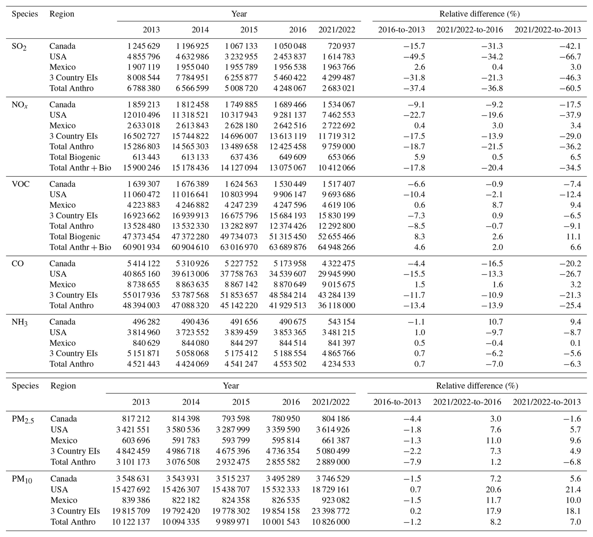
Some significant changes are evident in annual emissions over this nine-year time period in Table 1, first over the four-year period from 2013 to 2016, then from 2016 to 2021/2022, and in total from 2013 to 2021/2022. For example, North American “Total Anthro” SO2 emissions decreased by 37 % from 2013 to 2016 and then by a further 37 % from 2016 to 2021/2022, for a total decrease of 60 % relative to 2013, while “Total Anthro” NOx emissions decreased by 19 %, 22 %, and 36 % for the same three periods. “Total Anthro” VOC and CO emissions also decreased over the three periods, by 8 %, 1 %, and 9 % for VOC emissions and by 13 %, 14 %, and 25 % for CO emissions. “Total Anthro” NH3 emissions, on the other hand, were nearly constant during the 2013–2016 period but then increased in Canada while decreasing in the US and Mexico in 2021/2022 for an overall domain-total decrease of 6 % from 2013 to 2021/2022.
Table 1 also compares SMOKE-processed, domain-total annual anthropogenic emissions with calculated domain-total annual biogenic emissions of NOx and VOCs. Biogenic NO emissions can be seen to have contributed 4 % of domain-total NOx emissions in 2013, rising to 6 % in 2021/2022 as anthropogenic NOx emissions decreased and biogenic NO emissions increased. By contrast biogenic VOC emissions contributed 78 % of domain-total VOC emissions in 2013, a much larger percentage, and then rose to 81 % in 2021/2022 as anthropogenic VOC emissions declined and biogenic VOC emissions increased. In addition, Table S1 in the Supplement compares the seasonal variation of the SMOKE-processed SET4.0.0 anthropogenic emissions for 32 model species and the biogenic emissions of four model species. Seasonal variations depend strongly on both the pollutant and its source types and can have markedly different cycles. For example, NH3 is primarily emitted by agricultural activities and can be seen to have a pronounced winter minimum and summer maximum, whereas seasonal emissions of two lumped model VOC species, ALD2 (acetaldehyde and higher aldehydes) and CRES (cresols and phenols), have a pronounced winter maximum and summer minimum consistent with their dominant source being residential wood combustion. For most anthropogenic species, however, seasonal variations were considerably smaller, including SO2, NO, and NO2. Although fossil-fuel power generation is important for both SO2 and NOx emissions, this suggests that at the continental scale the increased power load for space heating in the winter in North America is roughly balanced by the increased power load for air conditioning in the summer. The seasonal variation of biogenic emitted species, on the other hand, was more like NH3; they had strong seasonal cycles with winter minima and summer maxima. In fact, biogenic isoprene (C5H8) emissions were predicted to have the most pronounced domain-level seasonal cycle, increasing from just 2 % in the winter to 65 % in the summer (Table S1).
2.3 Air-chemistry and precipitation-chemistry observations
Routine air-chemistry and precipitation-chemistry measurements are available from multiple measurement networks operating in Canada and the US. The hourly measurements of abundances of NO2, O3, and PM2.5 total mass made by continuous instruments that are reported in near-real time by some agencies to the US EPA's AirNow program (Dye et al., 2004; Wayland et al., 2004; Zhang et al., 2012a) have already been mentioned. AirNow hourly measurement data for NO2, O3, and PM2.5 from US monitors have been combined in this study with NRT NO2, O3, and PM2.5 hourly measurement data from Canadian National Air Pollution Surveillance (NAPS) monitors that report directly to ECCC's Canadian Meteorological Centre (CMC). This combined NRT data set has been used to evaluate the 2021/2022 RAQDPS-OP023 and RAQDPS-FW023 operational forecasts of these species.
The use of these NRT abundance measurements, which are considered to be preliminary, for model evaluation is consistent with the operational nature of the RAQDPS-OP023 forecasts. Two automated data filters were applied by CMC to the AirNow and NAPS NRT measurements upon receipt before they were used for model evaluation or other purposes such as operational air pollutant objective analyses (e.g., Robichaud et al., 2016). The first filter flagged negative abundance values and above-threshold abundance values as suspicious (NO2 levels over 200 ppbv, O3 levels over 200 ppbv, PM2.5 levels over 300 µg m−3) or invalid (NO2 levels over 2000 ppbv, O3 levels over 500 ppbv, PM2.5 levels over 1000 µg m−3), while the second filter flagged large jumps in abundances between consecutive hours as suspicious (over 30 ppbv for NO2, over 60 ppbv for O3, over 90 µg m−3 for PM2.5). Values flagged as suspicious or invalid were not used for this study. Measurements from stations located near roadways were discarded as well to ensure spatial representativeness. A temporal completeness criterion was also imposed on this NRT measurement data set to ensure temporal representativeness of the evaluation data: individual station data sets were required to have at least 75 % valid values out of the total possible values for a one-year evaluation period to be considered complete. More details about these representativeness constraints are provided in Sect. S2.4. Table 2 lists the number of available AirNow and NAPS stations for 2021/2022 that measured hourly O3, NO2, and PM2.5 abundances and the number with complete data records while Fig. S2 shows the locations of all stations measuring each of these three species. Note that some stations only measured one or two of these species.
Table 2Total number of US and Canadian measurement stations with complete hourly NO2, O3, and PM2.5 measurements for an annual evaluation vs. available measurements by network and year for 2013–2016 (AQS, NAPS) and 2021/2022 (AirNow, NAPS).
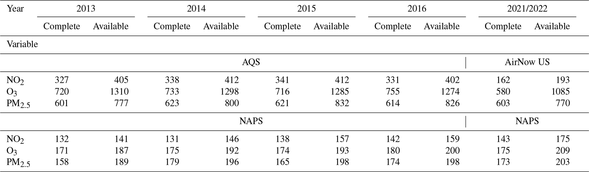
The evaluation of the retrospective annual simulations for 2013–2016, on the other hand, was based on finalized AQ network data sets. The CAPMoN and NAPS networks in Canada and the AMoN, AQS, CASTNET, CSN, IMPROVE, NATTS, and PAMS networks in the US provide finalized air-chemistry measurement data sets for various chemical species, including hourly NO2, O3, and other gas-phase species (e.g., SO2, CO, HNO3, NH3, ethene (C2H4), formaldehyde (HCHO), and C5H8), hourly PM2.5 and PM10 mass, daily FRM (Federal Reference Method) and FEM (Federal Equivalent Method) PM2.5 mass (e.g., Demerjian, 2000; Noble et al., 2001; Gantt, 2022), and daily PM2.5 chemical composition, while the CAPMoN network in Canada and the NADP network in the US provide finalized precipitation-chemistry measurement data sets. Details about each of these networks are given in Table S2a, and Sect. S2.3 provides some additional information about daily PM2.5 measurements. Note that all network data sets used in this study were accessed on 24 June 2024 (relevant because these data sets are always subject to change even years after their original release). Table 2 and S2b–d list the number of stations for each network for 2013–2016 with available measurements and with complete measurements of various chemical species (see Sect. S2.4), while Figs. S3–S6 show the locations of available stations by network. It is clear from these four figures that spatial coverage varies widely by the species being measured.
Although AQ measurements provide important chemical information about the real atmosphere, these measurements, like AQ model predictions, also have biases and errors. For example, NO2 measurements made with chemiluminescence monitors frequently have positive biases due to interference from other oxidized nitrogen species (e.g., Dunlea et al., 2007; Lamsal et al., 2015; Dickerson et al., 2019), and NH3 measurements made with passive monitors have negative biases (Puchalski et al., 2011). Measurements of both PM2.5 total mass and semi-volatile PM2.5 chemical components are known to have both positive and negative artifacts (e.g., Chow, 1995; Frank, 2006; Watson et al., 2009; Dabek-Zlotorzynska et al., 2011; Malm et al., 2011; Su et al., 2018; Gantt, 2022). Estimates of reconstructed PM2.5 total mass based on the sum of PM2.5 chemical component mass measurements from the CSN, IMPROVE, and NAPS networks often differ from direct measurements of PM2.5 total mass (e.g., Malm et al., 2011; Chow et al., 2015; Hand et al., 2019). As well, different networks measuring the same species often do not use the same instruments or follow the same field and laboratory protocols, which can affect comparability across networks. Examples include the use of different instruments to measure SO2, CO, and O3 concentrations by different agencies reporting to AQS (e.g., Demerjian, 2000; Parrish and Fehsenfeld, 2000), SO2 and HNO3 concentrations measured by the CAPMoN and CASTNET networks vs. the NAPS network (Dabek-Zlotorzynska et al., 2011; Feng et al., 2020), NH3 concentrations measured by the AMoN and NAPS networks (Dabek-Zlotorzynska et al., 2011; Puchalski et al., 2011), sulphur and nitrogen species measured by the CASTNET and IMPROVE networks (e.g., Ames and Malm, 2001; Lavery et al., 2009), and PM2.5 chemical components measured by the IMPROVE and CSN networks (Hand et al., 2012; Solomon et al. 2014). In order to assess measurement comparability between networks some efforts have been made to co-locate instruments used by different networks at one or more locations, including CSN and IMPROVE (Malm et al., 2011; Hand et al., 2012), CASTNET and CAPMoN (Schwede et al., 2011), and CAPMoN and NADP (Sirois et al., 2000; Wetherbee et al., 2010; Feng et al., 2023).
2.4 Pairing measurements with model predictions
The comparison of AQ measurements and AQ model predictions must be done with care since measurements and model predictions never represent exactly the same quantities (e.g., Seigneur and Moran, 2004; Appel et al., 2008). From a temporal perspective, reported AQ measurements may either be instantaneous values or time averages, and the time averages may in turn represent mean values for an averaging period that begins, ends, or straddles the reporting time. Model values, on the other hand, are nominally instantaneous but correspond to a time that is a discrete time step after the previous integration time and after a particular operator calculation step in a repeating sequence of numerical operators. From a spatial perspective, AQ measurements are typically made at a near-surface “point” location whereas AQ model predictions represent a volume-average value corresponding to the volume of an individual model grid cell. This spatial representativeness discrepancy is sometimes referred to as incommensurability. It is a fundamental source of model uncertainty that can be reduced by reducing model grid spacing but never removed entirely (e.g., Nappo et al., 1982; Venkatram, 1988; McNair et al., 1996; Spicer et al., 1996; Swall and Foley, 2009; Stroud et al., 2011; Schutgens et al., 2016). Estimates of population exposure to air pollutants based on ambient measurements from a small number of AQ measurement stations also suffer from the same problem (e.g., Jerrett et al., 2005; Hystad et al., 2011). And lastly, from a chemical perspective AQ measurements sometimes correspond to a combination of two or more model variables while in other cases they correspond to more detailed chemical species than the AQ model is able to consider. For these reasons some pre-processing is generally required to pair or match AQ measurements and model predictions before they are compared while bearing in mind that some differences will still remain. It is thus important to document the methodology used to perform this pairing (Simon et al., 2012).
Temporal pairing was relatively straightforward for this study, although it was necessary to examine AQ network documentation carefully to understand the exact temporal nature of the measurements being reported. Model abundance predictions were available every chemistry time step, or every 15 min in the case of the RAQDPS-OP023 (Moran et al., 2026), so it was simple to pair model predictions with instantaneous hourly abundance measurements. On the other hand, to pair model predictions with the mean hourly abundance measurements reported by the NAPS and AQS networks (Fig. S2), multiple consecutive sub-hourly model predictions needed to be combined using one of two approaches: an end-value approach, which averages the model values at the beginning and end of the measurement sampling period; or an integration approach, where the trapezoidal rule is used to combine the five RAQDPS-OP023 values available for the hour. The end-value approach was used in this study. To pair model predictions with mean daily air abundance measurements from the AQS, CSN, IMPROVE, and NAPS networks (Table S2a), all hourly model values for each 24 h sampling period were averaged. To pair with mean weekly air abundance measurements from CASTNET, all hourly model values for each weekly sampling period were averaged; the same weekly averaging was also performed for daily mean CAPMoN and NAPS air concentrations for temporal consistency in order to be able to compare evaluation statistics between networks properly and to pool measurements for these three networks. Similarly, to pair model predictions with mean biweekly AMoN abundance measurements, hourly model NH3 values were averaged for each biweekly sampling period, and the same was done for NAPS daily mean NH3 values for temporal consistency. Finally, to pair model predictions with daily precipitation-chemistry measurements (CAPMoN) or weekly precipitation-chemistry measurements (NADP), hourly model wet deposition forecasts were accumulated for the appropriate period, but then weekly deposition values were also calculated for CAPMoN for temporal consistency with NADP. Weekly precipitation-weighted mean wet concentration values were then calculated from weekly precipitation and weekly deposition values.
More details about pairing related to this study, including spatial and chemical considerations, especially for PM measurements, and completeness screening, are provided in Sect. S2.4. These include the nuances of evaluating VOC predictions, handling ambient vs. standard temperature and pressure, the measurement proxies used for some PM chemical components such as NH4, total organic matter (TOM = POM + SOM), CM, and SS, the treatment of aerosol water, and the combined gas-particle phases implicit in precipitation-chemistry measurements. For example, one important consideration related to pairing with VOC measurements is that while measurements of ethene (C2H4) are available, the ADOM-2 model VOC species named ETHE is a lumped species that includes additional VOC species (Sect. S2.4). This misalignment must be considered when interpreting evaluation results for ETHE in Sect. 3.3.1 since the measurements are in effect lower bounds on the model predictions of this species rather than direct counterparts.
2.5 Model performance metrics and evaluation
Once a set of paired observed and model-predicted values is available, model performance metrics can be calculated. For the present study we chose to calculate 12 statistical metrics: observation mean (); model prediction mean (); mean bias (MB); normalized mean bias (NMB); normalized mean absolute error (NMAE); root mean square error (RMSE); Pearson correlation coefficient (R); fraction of predictions within a factor of 2 of observations (FAC2); centered root mean square error (CRMSE); standard deviations of observations (σO or SDO) and model predictions (σM or SDM); and normalized standard deviation (NSD). Definitions of these metrics are provided in Table A2 and some background information about their selection is provided in Sect. S2.5. Inclusion of the first seven of these metrics is consistent with the recommendation of Simon et al. (2012) for a minimum set of performance evaluation statistics that should always be calculated to promote comparability across separate studies. The eighth metric, FAC2, is a dimensionless and bounded (0–1) measure of error or scatter that is not sensitive to outliers (e.g., Chang and Hanna, 2004; Borrego et al., 2008; Derwent et al., 2010; Savage et al., 2013). CRMSE, unlike RMSE, is insensitive to bias and represents the error due to differences in pattern variation or, alternately, the standard deviation of the error; it has been used in many studies (e.g., Bencala and Seinfeld, 1979; Stanski et al., 1989; Taylor, 2001; Chang and Hanna, 2004; Entekhabi et al., 2010; Sakaguchi et al., 2012; Thunis et al., 2012). NSD has been suggested as a metric by Taylor (2001), Chang and Hanna (2004), and Thunis et al. (2012), but by itself it does not provide information about the magnitudes of σO or σM (which were recommended by Willmott, 1981 and reported by Appel et al., 2021). Note that CRMSE, R, σO, and σM (and sometimes NSD) are all linked by the Taylor diagram (Taylor, 2001). One other quantity that should be reported with these 12 metrics is N, the number of measurement-model pairs. Many evaluation studies fail to report this quantity, but it is used explicitly in the calculation of many metrics and it provides valuable information about sample size, representativeness, and significance (e.g., Huang et al., 2021).
Since this is an AQ forecasting evaluation, we have focused here on “native” network sampling duration: that is, hourly, daily, weekly, or biweekly samples, but based on the networks with the longest sampling duration for each species (e.g., biweekly for AMoN for NH3, but weekly for CASTNET and NADP-NTN) to allow consistent comparisons between networks and pooling of network measurements. Other studies that focused on model performance for regulatory applications have looked at “constructed” predictands such as maximum daily 8 h average (MDA8) or maximum 1-hourly values of O3 volume mixing ratios (VMRs), whereas in this study we have only considered network-reported values such as hourly O3 VMRs. And while we report annual domain-average statistics based on combined network measurements, we also report results for more stratified (i.e., disaggregated) analyses, including network-specific statistics, seasonal statistics, monthly statistics, diurnal statistics, regional statistics, and urban/rural statistics. To calculate urban vs. rural statistics, each measurement site was classified as urban or rural based on its grid-cell population density, where a threshold of 400 persons per km2 was applied for Canada and 386 persons per km2 (1000 persons per square mile) for the US as the minimum urban population density. The slightly different thresholds were used for consistency with national censuses. We have also discussed our statistical results contextually in the next wo sections by referring to the performance benchmarks proposed by Simon et al. (2012), Emery et al. (2017), Kelly et al. (2019), Huang et al. (2021), and Zhai et al. (2024) (see Sect. S2.5). Some additional discussion related to model performance metrics is provided in Sect. S2.5.
This section presents performance evaluation statistics, first for one meteorological parameter that is important for air quality (Sect. 3.1), then for three key chemical species, NO2, O3, and PM2.5 total mass (Sect. 3.2), and then for other gas-phase species, PM2.5 chemical composition, and wet concentration and deposition of three inorganic species (Sect. 3.3). Annual, seasonal, monthly, diurnal, and regional evaluations for the one-year period from 1 June 2021 to 31 May 2022, the first year of RAQDPS-OP023 forecasts, are presented in this section along with selected evaluation results for the 2013–2016 RAQDPS-OP023 annual simulations. Many additional tables and figures related mainly to the 2013–2016 simulations, which serve to further quantify predictive skill and characterize the temporal and spatial variability of RAQDPS-OP023 performance, can be found in Sect. S3.
3.1 Operational evaluation of AQ-relevant meteorological predictands
Meteorological processes affect air quality through their influence on emissions, atmospheric transport and diffusion, chemistry, and wet and dry removal. Near-surface temperature, wind speed, and precipitation are three meteorological parameters that are important for surface air quality (e.g., Vautard et al., 2012; Gilliam et al., 2015; McNider and Pour-Biazar, 2020; Wang et al., 2021; Campbell et al., 2022). As described in the companion paper by Moran et al. (2026), the RAQDPS-OP023 (and RAQDPS-FW023) is a regional chemical weather model configured to produce nearly identical meteorological forecasts to the RDPS 8.0.0, the ECCC regional weather forecast model that was operational at the same time (Fillion et al., 2010; Caron et al., 2015; McTaggart-Cowan et al., 2019; CMC-RDPS-8.0.0, 2021). Performance evaluations of RDPS weather forecasts have been presented in these and other publications. For this paper we have only evaluated RAQDPS-OP023 precipitation forecasts based on precipitation measurements from precipitation-chemistry networks, which are not usually available to or considered in NWP model performance evaluations. This choice also ensures that performance statistics for precipitation are consistent in time and space with those for pollutant concentrations in precipitation and wet deposition (Sect. 3.3.3).
Domain-average annual scores for RAQDPS-OP023 weekly precipitation forecasts at precipitation-chemistry stations for 2013 to 2016 are listed in Table 6. As noted in Sect. 2.4 we have chosen to consider weekly forecasts because the US NADP precipitation-chemistry network only reports weekly accumulated measurements. Interestingly, this set of scores does not show much variation from year to year. For example, annual MB values ranged from −0.1 to 2.2 mm per week, NMB values from −0.01 to 0.12, NMAE values from 0.49 to 0.54, RMSE values from 17.6 to 20.6 mm per week, FAC2 values from 0.56 to 0.57, and R values from 0.71 to 0.78. Appel et al. (2011) reported a comparable NMB range but a markedly lower RMSE range for 12 km MM5 meteorological model simulations for the 2002–2006 period, but those earlier statistics were calculated for accumulated seasonal and annual precipitation predictions as opposed to weekly predictions, which have greater temporal variability.
Seasonal analyses of RAQDPS-OP023 predictions of near-surface temperature, wind speed, and precipitation can be found in Sect. S3.1 as well as individual-network annual and seasonal evaluation scores and subregional annual evaluation scores for weekly precipitation. These additional evaluations showed that model skill in predicting weekly precipitation was highest for the winter season and lowest for the summer season (e.g., Fig. S161). The probable explanation is that organized, synoptic-scale precipitation, which is more predictable, is likeliest to occur in the winter whereas small-scale convective precipitation, which is harder for NWP models to predict, is likeliest to occur in the summer (e.g., Appel et al., 2011; Gilliam et al., 2021). Many of the largest overpredictions of weekly precipitation at individual stations occurred in the Rocky Mountain region of the western US, where station location relative to subgrid-scale (SGS) topographical features is likely to be important, whereas underpredictions at stations were common in the flatter terrain of the southeastern and central US (Fig. S121). In addition, the evaluation statistics for an individual network or month or subregion were sometimes qualitatively different from those for the combined networks, combined months, or combined subregions. For example, model skill in predicting annual and seasonal mean weekly precipitation was found to be higher for the Canadian CAPMoN precipitation-chemistry network than the US NADP network (Tables S6A and S6S). This possibility always needs to be kept in mind when interpreting the most highly aggregated performance statistics (e.g., annual statistics and all-network, all-station statistics), which may obscure systematic network differences or be impacted by compensating errors (e.g., Makar et al., 2014).
3.2 Operational evaluation of three key air quality predictands
This section presents operational evaluation results for RAQDPS-OP023 predictions of hourly surface NO2, O3, and PM2.5 total mass abundances for five years. Results are presented first for 2021/2022 NO2 and O3 forecasts that were compared to NRT measurements, followed by results for 2013–2016 NO2 and O3 hindcasts that were compared to QA/QCed network measurements, 2021/2022 PM2.5 forecasts compared to NRT measurements, and 2013–2016 PM2.5 hindcasts compared to QA/QCed network continuous and gravimetric measurements.
3.2.1 NO2 and ozone
2021/2022 operational forecasts of NO2 and O3
Figure 1 shows the spatial distribution over North America of annual mean NO2 and O3 hourly surface VMR fields predicted by the RAQDPS-OP023 for the 2021/2022 period. Coloured “coffee beans” (i.e., divided dots) are superimposed on the contoured fields to show observed and predicted annual mean values at NRT measurement stations for the same period (see Fig. S2 for station locations). Generally good agreement is evident in Fig. 1 between the observed and predicted annual mean values of both pollutants (although viewing the NO2 panel with higher magnification is helpful); note that the higher NO2 VMRs associated with urban centers are smaller-scale features caused by high NOx emissions over urban centers (cf. Fig. S1a in the Supplement).
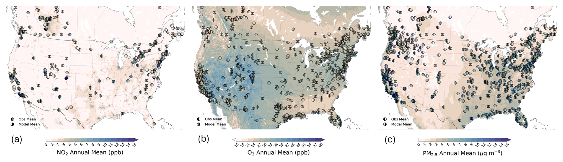
Figure 1Spatial distribution of RAQDPS-OP023-predicted 2021/2022 annual-mean abundance fields of hourly (a) NO2 VMR, (b) O3 VMR, and (c) PM2.5-noSS concentration with NRT observed and predicted station annual abundances superimposed (shown as filled-in divided circles, same colour bar). Units are ppbv, ppbv, and µg m−3, respectively.
More quantitatively, Table 3 lists values of all-station annual model evaluation statistics for hourly NO2 and O3 VMR forecasts for 2021/2022. These overall performance scores are generally less good for NO2 than for O3, including NMB (−0.19 vs. −0.07), NMAE (0.56 vs. 0.28), FAC2 (0.52 vs. 0.83), and R (0.65 vs. 0.72). This difference is not surprising given that NO2 is a primary pollutant whose spatial distribution is dominated by the distribution of emissions with strong spatial gradients whereas O3 is a secondary pollutant with a smoother spatial pattern and smaller dynamic range. One indicator of the degree of smoothness of a pattern is the coefficient of variation (CV) or relative standard deviation (ratio of standard deviation to arithmetic mean; see Table A2), where a lower value indicates a smoother field (i.e., lower variability) (e.g., Fruin et al., 2014; Lee et al., 2018). The observed and predicted annual CV values for 2021/2022 calculated from Table 3 were 1.16 and 1.20, respectively, for NO2 vs. 0.50 and 0.47 for O3.
Table 3Summary table of all-station annual statistics for the RAQDPS-OP023 for hourly NO2, O3, and PM2.5 surface measurements for 2021/2022 and 2013–2016. For dimensional statistics, units are ppbv for NO2 and O3 and µg m−3 for PM2.5.
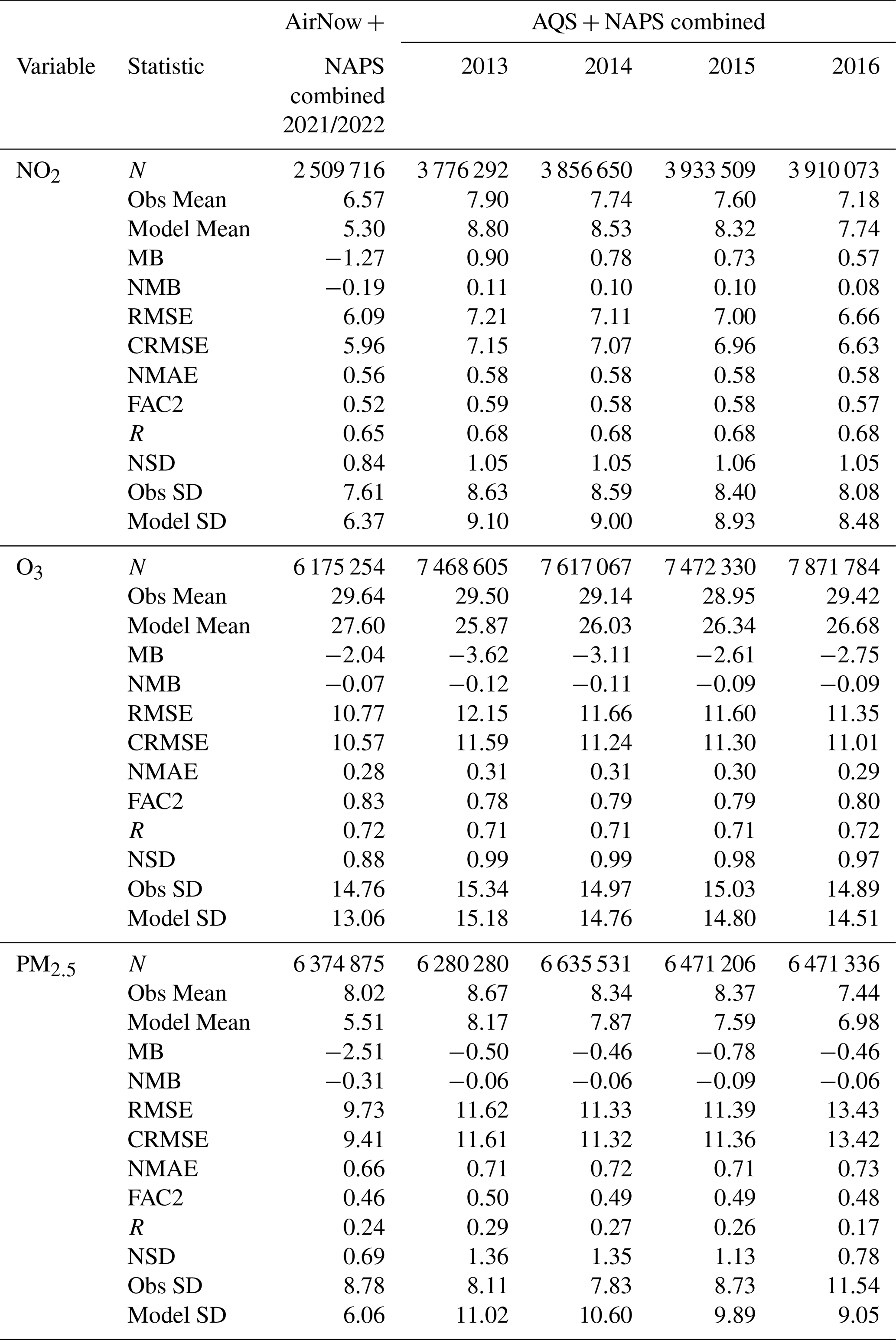
In order to judge the level of model skill suggested by the Table 3 scores, Zhai et al. (2024) have recommended benchmark goals for NMB, NMAE, and R of ±0.20, 0.40, and 0.60 for “good” NO2 performance scores (i.e., scores above 67th percentile relative to the scores for a historical multi-model ensemble) while Emery et al. (2017) have recommended benchmark goals for NMB, NMAE, and R of ±0.05, 0.15, and 0.75 as good O3 performance scores. These benchmark goals were met by RAQDPS-OP023 forecasts for 2021/2022 for NO2 except annual NMAE scores but not for O3 annual scores.
When interpreting these benchmark comparisons, however, it should be noted that Emery et al. (2017) also recommended that the evaluation period considered should be no more than one month for O3 and a 40 ppbv cutoff should be used when calculating NMB and NMAE for O3, whereas no cutoff was considered for Table 3. In addition, Simon et al. (2012) found performance scores for retrospective model applications to be better on average than those for forecast applications due to the use by the former of year-specific emissions, meteorological reanalyses, day-specific chemical lateral boundary conditions, and other retrospective data sets that are not available to AQ forecasting applications. It was also noted in Sect. 2.3 that most network NO2 monitors in North America suffer from positive biases due to interference from other oxidized nitrogen species (e.g., Dunlea et al., 2007; Dickerson et al., 2019). These biases, however, vary greatly with time and location. They are expected to be smallest when fresh NO2 emissions dominate, for example, in urban areas, in the early morning hours (04:00–09:00 LT) when the PBL is shallow, and in the winter, but largest relatively speaking for aged air, as in rural areas, in the afternoon hours, and in the summer (e.g., Godowitch et al., 2010; Lamsal et al., 2015; Jaeglé et al., 2018; He et al., 2019; Toro et al., 2021). Thus, the annual NMB value for NO2 of −0.19 would be smaller if these measurement biases were accounted for.
Figures 2 and 3 provide an extreme disaggregation of the all-station annual scores from Table 3 by showing spatial distributions of station-specific annual values of four statistics (MB, NMB, CRMSE, and R) for hourly NO2 and O3 measurements, respectively, for 2021/2022. Such plots can reveal regional patterns in the evaluation statistics. For example, annual NMB values for NO2 tend to be negative everywhere (again consistent with a positive measurement bias) but they are more negative (i.e., worse) in general at western stations while CRMSE and R values for NO2 are lower in the continental interior than in coastal areas (Fig. 2). Annual MB and NMB values for O3, on the other hand, are generally negative at western stations but positive at eastern stations, particularly at coastal stations (Fig. 3), while both annual CRMSE and R scores are higher overall across the continent for O3 than for NO2.
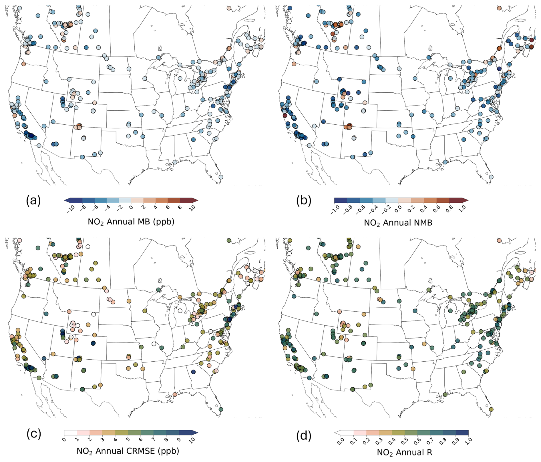
Figure 2Spatial distribution of 2021/2022 annual (a) MB, (b) NMB, (c) CRMSE, and (d) R scores for the RAQDPS-OP023 at all NRT stations for hourly NO2 VMR measurements (ppbv).
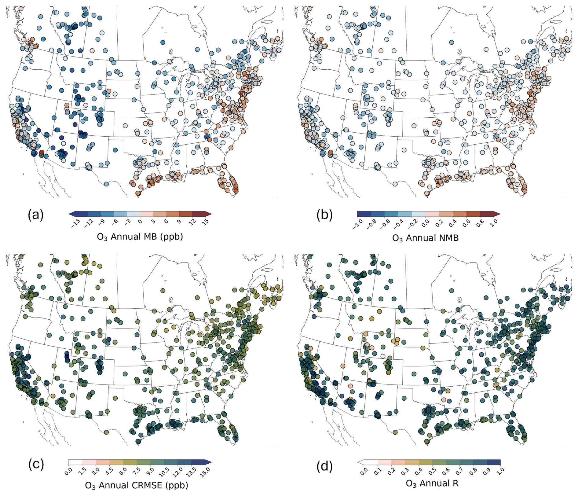
Figure 3Spatial distribution of 2021/2022 annual (a) MB, (b) NMB, (c) CRMSE, and (d) R scores for the RAQDPS-OP023 at all NRT stations for hourly O3 VMR measurements (ppbv).
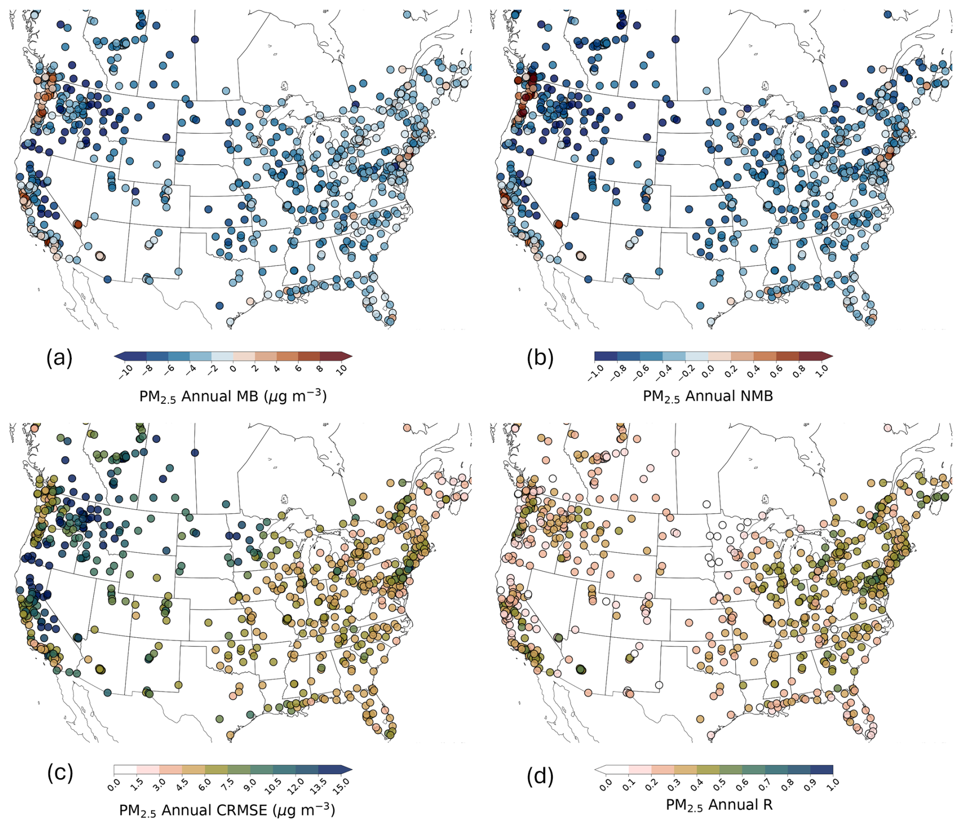
Figure 4Spatial distribution of 2021/2022 annual (a) MB, (b) NMB, (c) CRMSE, and (d) R scores for the RAQDPS-OP023 at all NRT stations for hourly PM2.5 concentration measurements (µg m−3).
Figure 5 adds temporal detail to the annual analysis shown in Fig. 1. It shows the corresponding predicted spatial distributions of seasonal mean NO2 and O3 hourly surface VMR fields for 2021/2022, again with superimposed coloured divided dots to show observed and predicted seasonal mean values at NRT measurement stations for each season. By inspection, predicted domain-scale, seasonal mean NO2 levels appear to be highest in the winter season (DJF) and lowest in the summer season (JJA), whereas O3 levels are predicted to be highest in the spring season (MAM) and lowest in the autumn (SON) season.
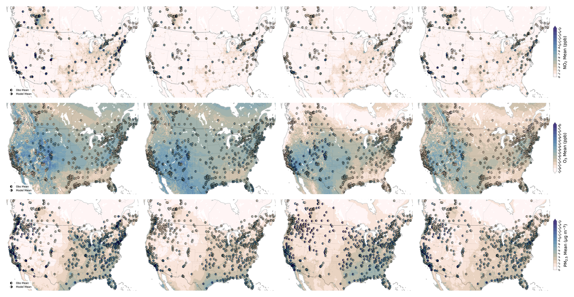
Figure 5Spatial distribution of RAQDPS-OP023-predicted 2021/2022 seasonal-mean abundance fields – from left to right: winter (DJF), spring (MAM), summer (JJA), autumn (SON) – of hourly (top row panels) NO2 VMR, (middle row panels) O3 VMR, and (bottom row panels) PM2.5-noSS concentration with NRT observed and predicted station seasonal abundances superimposed (shown as filled-in divided circles, same colour bar). Units are ppbv, ppbv, and µg m−3, respectively.
Another perspective on the temporal variation of RAQDPS-OP023 performance is provided by Figs. 6 and 7, which show time series of observed and predicted all-station monthly mean VMR values of hourly NO2 and O3, respectively, for 2021/2022 for all NRT measurement stations in the model domain. Time series of monthly NMB, CRMSE, and R scores are also shown in these two figures. Observed and predicted monthly mean NO2 VMRs are both highest in January and lowest in June and July; observed and predicted monthly mean O3 VMRs are both highest in April and lowest in November. Monthly NMB values for hourly NO2 are negative for all months but are slightly worse for the winter months even though the NO2 measurement bias is expected to be smaller in the winter, while monthly CRMSE values for NO2 peak in January, and monthly R values for NO2 do not vary much from month to month but are slightly higher in the winter. Monthly NMB values for hourly O3 are negative for all months except December and January, monthly CRMSE values for O3 peak in July, and monthly R values for O3 also do not vary much but are slightly higher in the summer. It should be noted that seasonal variations in NOx emissions are very small at the domain scale (Table S1), suggesting that the observed and predicted variations in monthly mean NO2 levels evident in Fig. 6 are controlled by factors other than emissions, such as monthly variations in temperature, photolysis, PBL height, vegetation phenology, and dry deposition. For O3, on the other hand, biogenic emissions of VOCs, its other main precursor, have very large seasonal variations (Table S1). Interestingly, although the largest predicted monthly O3 values occur in April, the model still underpredicts the well-known springtime O3 maximum in the Northern Hemisphere (e.g., Penkett and Brice, 1986; Monks, 2000; Liudchik et al., 2015) by about 5 ppbv in April.
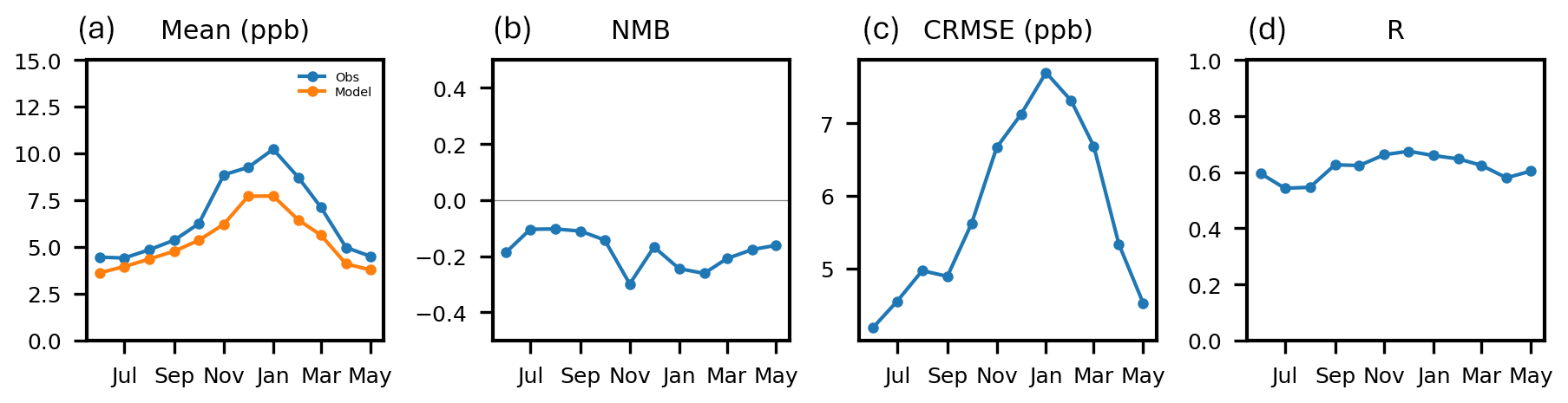
Figure 6Time series of (a) observed and RAQDPS-OP023-predicted monthly means of hourly NO2 VMR (ppbv) and monthly (b) NMB, (c) CRMSE, and (d) R scores for 2021/2022 for all NRT measurement stations.
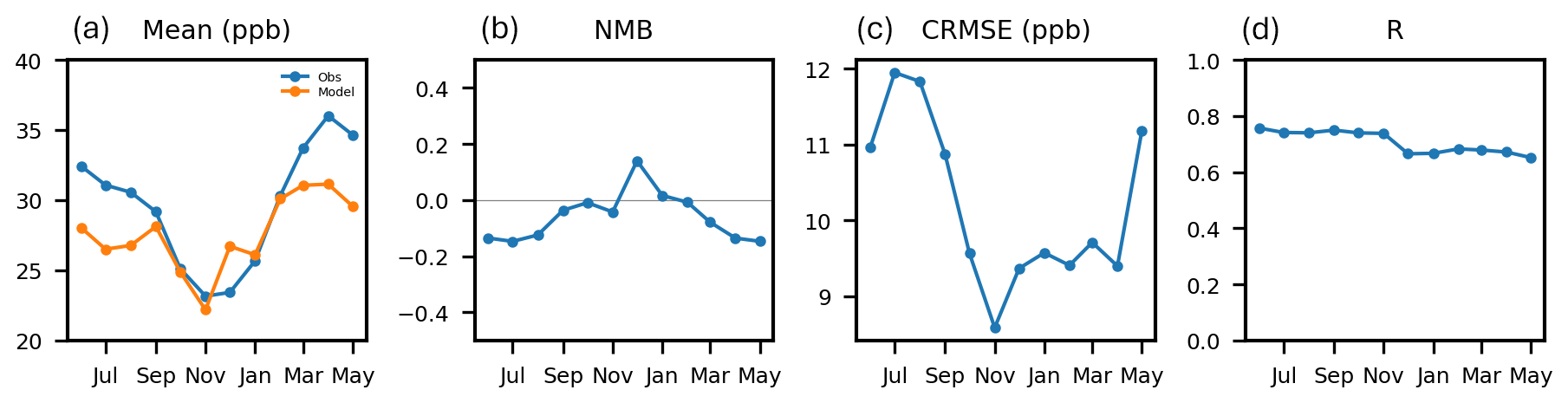
Figure 7Time series of (a) observed and RAQDPS-OP023-predicted monthly means of hourly O3 VMR (ppbv) and monthly (b) NMB, (c) CRMSE, and (d) R scores for 2021/2022 for all NRT measurement stations.
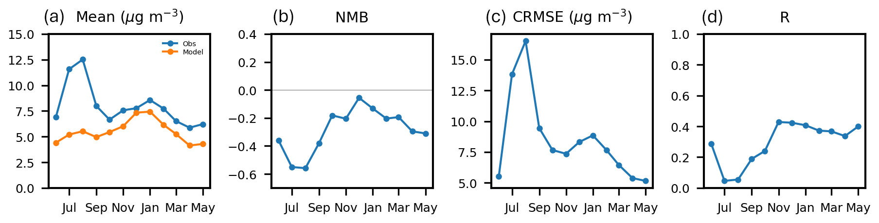
Figure 8Time series of monthly (a) observed and RAQDPS-OP023-predicted mean hourly PM2.5 concentration (µg m−3) and (b) NMB, (c) CRMSE, and (d) R scores for 2021/2022 for all NRT measurement stations.
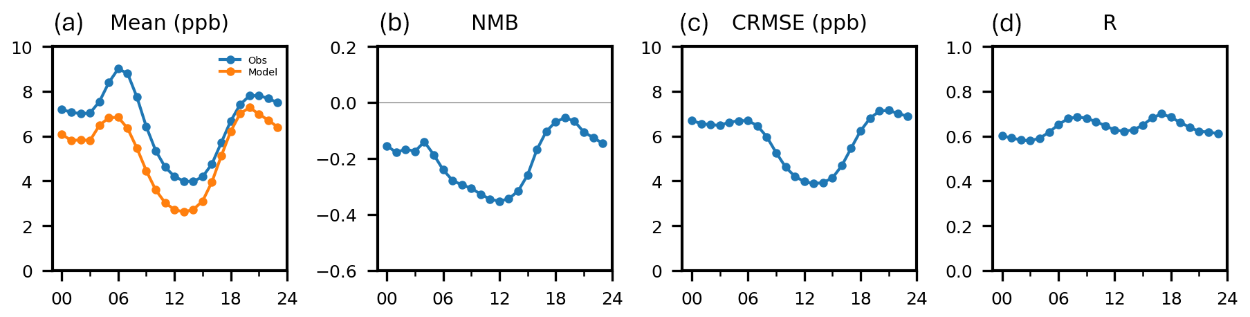
Figure 9Time series of diurnal (a) observed and RAQDPS-OP023-predicted annual-mean hourly NO2 VMR (ppbv) and (b) NMB, (c) CRMSE, and (d) R scores for all of 2021/2022 for all NRT stations. Time is in hours LT.
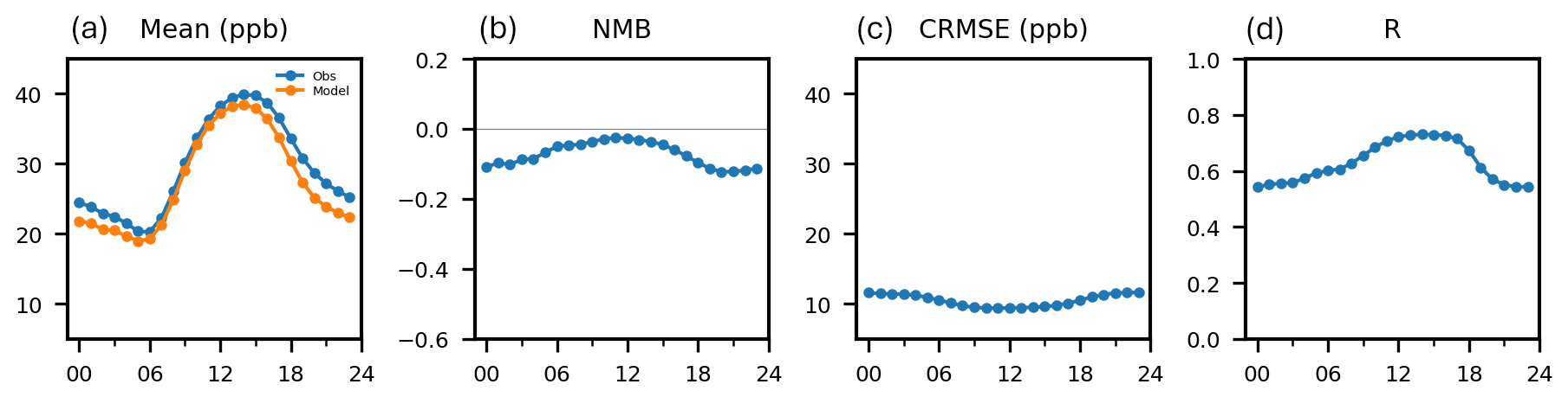
Figure 10Time series of diurnal (a) observed and RAQDPS-OP023-predicted annual-mean hourly O3 VMR (ppbv) and (b) NMB, (c) CRMSE, and (d) R scores for all of 2021/2022 for all NRT stations. Time is in hours LT.
It is also of interest to examine RAQDPS-OP023 performance by time of day since many emission source sectors and meteorological and chemical processes vary diurnally. Figures 9 and 10 show all-station, annual-mean diurnal time series in local time (LT) of values of five statistics for hourly NO2 and O3 surface VMRs, respectively, for the 2021/2022 period. The annual-mean diurnal time series of observed and predicted hourly VMRs for both species display a strong dependence on time of day as do the diurnal time series of annual NMB, CRMSE, and R scores. Model predictions of annual-mean hourly values of both NO2 and O3 surface VMRs agree well overall with observations, including the times of the observed daily maxima and minima. The annual-mean diurnal time series of hourly NO2 VMR and the associated hourly evaluation statistics in Fig. 9 display extrema close to the times of morning and afternoon rush hours, suggesting that diurnal variation of on-road NOx emissions plays an important role in driving the diurnal pattern. Interestingly, hourly NMB values for NO2 are most negative in the afternoon when the NO2 measurement bias is expected to be largest. By contrast, the maximum annual-mean hourly O3 VMR occurs at 14:00 LT and the minimum at 05:00 LT (Fig. 10). For O3 the smallest annual-mean hourly NMB and CRMSE values and highest annual-mean hourly R values occur close to the mid-day O3 peak.
Figures 2–4 showed how model performance can vary geographically. A complementary result is presented in Fig. 12, which compares regional time series of observed and RAQDPS-OP023 predicted monthly means of hourly NO2 and O3 VMRs for 2021/2022 for the four continental quadrants shown in Fig. S7. Both observed and predicted time series exhibit a regional dependence. For NO2 the agreement between observed and predicted monthly means was closest for western Canada while for O3 it was closest for the eastern US. Peak observed monthly mean NO2 VMR values were slightly higher in the west than in the east, at least for these regional sets of stations (see Fig. S2). Observed and predicted monthly mean NO2 VMR peaks also occurred in January in three of the four regions and in December in the eastern US, in overall agreement with Fig. 6. Note too that monthly mean NO2 VMRs were also underpredicted in all months in the western and eastern US, in agreement with Fig. 6, but some monthly overpredictions can be seen in western and eastern Canada. Peak observed monthly mean O3 VMR values occurred in April in three of the four regions, in agreement with Fig. 7, but in July in the western US. Peak predicted monthly mean O3 VMR values, on the other hand, occurred in March or April, and both underpredictions and overpredictions of monthly mean O3 VMR are evident in Fig. 12 in all four regions.
2013–2016 hindcasts of NO2 and O3
The RAQDPS-OP023 annual hindcasts for 2013–2016 can also be evaluated to look for consistencies in model performance across multiple years. Figure 13 shows plots of predicted spatial distributions of annual mean NO2 and O3 surface VMR fields for 2013–2016 and 2021/2022. For both species the broad spatial patterns are very similar over land for the five years despite year-to-year variations in meteorology and the monotonic decrease of 18 % in domain-total NOx emissions over the 2013–2016 period and the further decrease of 20 % from 2016 to 2021/2022 (Table 1). Nevertheless, year-to-year decreases in annual NO2 levels are visible over this near-decadal period, including in Texas, the Ohio Valley, and the Washington, D.C.–Boston corridor. Latitudinal gradients in the spatial distributions of O3 surface VMR can be seen over land in Fig. 13 for all five years, with a east-west band of elevated values stretching across the continental US and peaking in the elevated terrain of the US Rocky Mountain and Great Basin regions. A recent analysis of winter and spring surface O3 observations over North America for 2010–2014 showed a similar pattern (Gaudel et al., 2018). However, trends in O3 from 2013 to 2021/2022 are not obvious in Fig. 13, unlike those for NO2.
Table 3 lists values of observed and RAQDPS-OP023-predicted all-station annual mean NO2 and O3 surface VMRs for 2013–2016 as well as 2021/2022. Note that the statistics for the 2013–2016 period are based on quality-assured, retrospective observation data sets released by individual agencies rather than the NRT measurements used to evaluate 2021/2022 forecasts (see Fig. S3 for station locations). Consistent with Fig. 13, observed and predicted all-station annual mean NO2 VMR values both exhibit a monotonic decrease from 2013 to 2021/2022, though for a smaller set of US stations in 2021/2022 (Table 2), whereas observed all-station annual mean O3 VMR values exhibit little change over this period vs. a small upward trend for predicted all-station annual mean O3 VMR. Table 3 also lists all-station annual values of 10 other model performance statistics for the five years. Statistics for the hindcasts might be expected to be better than the forecasts due to the use of year-specific emissions. In fact, the scores are mixed and are comparable overall for the five years. For example, annual NMB values for NO2 VMR are negative for 2021/2022 but positive and smaller in magnitude for the other four years, annual RMSE and NMAE values for NO2 VMR are better for 2021/2022 than for 2013–2016, but FAC2 and R values for NO2 VMR are better for 2013–2016 than for 2021/2022. The annual NMB and R values for NO2 VMR for 2013–2016 all meet the benchmark goals of ±0.20 and 0.60 for good performance recommended by Zhai et al. (2024), similar to 2021/2022, but annual NMAE scores for 2013–2016 do not meet either of their recommended thresholds (0.40 or 0.55). Annual NMB values for O3 VMR, on the other hand, are more negative for 2013–2016 than for 2021/2022 and FAC2 scores are also lower while NMAE and R scores are comparable. In addition, the annual NMB and R scores for O3 VMR for 2013–2016 all meet the acceptable benchmarks of ±0.15 and 0.50 for these statistics recommended by Emery et al. (2017), similar to 2021/2022, but fall below the more stringent benchmark goals of ±0.05 and 0.75, while NMAE scores for 2013–2016 do not meet either recommended threshold (0.15 or 0.25).
Additional analyses
Results from additional data analyses for NO2 and O3 with a focus on the 2013–2016 RAQDPS-OP023 hindcasts can be found in Sect. S3.2.1. These results include tables of separate annual and seasonal scores for the AQS and NAPS networks as well as seasonal and regional diurnal analyses for 2021/2022, regional scores for all five years, spatial plots of both annual station scores and predicted seasonal mean surface VMR fields for 2013–2016, and monthly time series, monthly density scatterplots, and urban vs. rural monthly time series for 2013–2016. One finding from these supplemental analyses is the high level of consistency between the aggregated annual statistical scores across years for both species for the AQS and NAPS networks individually (Table S3A) and annual scores at the individual station level (e.g., Fig. S42). Another is the clear consistency across the 2013–2016 hindcasts of the seasonal variations in the NO2 and O3 seasonal mean VMR fields, statistical scores, and monthly mean time series (e.g., Table S3S, Fig. S11), which helps to identify systematic model errors. Third, the overall agreement in observed and predicted temporal trends also provides support for the representativeness of the year-specific emissions used for these hindcasts (e.g., Fig. S140). Fourth, there are some striking differences between the time series of monthly NO2 and O3 statistics for urban stations vs. rural stations that underline the importance of emissions forcing, including higher NO2 levels and lower O3 levels in urban areas (e.g., Fig. S209 vs. Fig. S210). Fifth, the annual regional analysis found that the two western regions had the largest negative NMB values for O3, consistent with Fig. 12 and pointing to possible issues with the O3 lateral boundary conditions for the western boundary (Table S7). Sixth, the monthly density scatterplots reveal an obvious precision limitation (only whole numbers) in the reported hourly NO2 measurements (Fig. S169).
A seventh finding was that annual, seasonal, and monthly negative NMB values were considerably larger for NO2 in the 2021/2022 forecasts for the two US regions (−0.31, −0.25) vs. the two Canadian regions (−0.06, −0.03). The same pattern was not seen in the 2013–2016 hindcasts, which used retrospective rather than projected emissions (Table S7). This is one example of the value of computing and then comparing statistics for the individual networks as well as the combined networks (e.g., Tables S3A and S3S). The differences in biases between countries found for the 2021/2022 forecasts might suggest that the US NOx emissions used for these forecasts were too low, whereas the Canadian NOx emissions that were used were more representative of 2021/2022 conditions. Since some time has passed since 2021 when the RAQDPS-OP023 became operational, retrospective national emissions inventories are now available for 2021 for both Canada and the US (ECCC, 2025a; US EPA, 2025). Interestingly, a comparison of these inventories with Table 1 showed that the projected annual NOx inventory emissions considered for both countries were in fact higher than the actual inventory values for 2021: 8 % higher for the US and 13 % higher for Canada. Other explanations must thus be sought.
3.2.2 PM2.5 total mass
2021/2022 operational forecasts of PM2.5 total mass
Figure 1 also shows the spatial distribution over North America of the annual mean PM2.5 hourly surface concentration field (without sea-salt component) predicted by the RAQDPS-OP023 for 2021/2022. Coloured divided dots are again superimposed to show observed and predicted annual values at NRT hourly PM2.5 measurement stations for the same period (see Fig. S2 for station locations). It is clear from this figure that the RAQDPS-OP023 underpredicts annual PM2.5 levels for 2021/2022 at a majority of measurement stations.
Table 3 lists values of observed and RAQDPS-OP023-predicted all-station annual mean PM2.5 surface concentrations (including the sea-salt component) and 10 other annual evaluation statistics for hourly PM2.5 forecasts for all stations measuring hourly PM2.5 (including both Class III FEM and non-FRM/FEM monitors: see Sect. S2.3 for more detaiils) for 2021/2022. All-station annual MB and NMB values for forecast hourly PM2.5 concentrations were −2.5 µg m−3 and −0.31, respectively, consistent with Fig. 1. Other statistics in Table 3 for PM2.5 were also poorer (e.g., NMAE = 0.66, FAC2 = 0.46, R=0.24, NSD = 0.69) than corresponding scores for NO2 and O3. Emery et al. (2017) proposed “acceptable” score benchmarks (i.e., above 33rd percentile for a historical multi-model ensemble) for predicted PM2.5 total mass for NMB, NMAE, and R scores of ±0.30, 0.50, and 0.40, but none of these benchmarks were met for the 2021/2022 hourly PM2.5 forecasts.
Figure 4 shows the spatial distribution of station-specific annual values of MB, NMB, CRMSE, and R for hourly PM2.5 total mass for 2021/2022 based on NRT hourly measurements at AirNow and NAPS stations. Consistent with Fig. 1 and Table 3, annual MB was negative for most stations, but values were small at a minority of stations and even positive at a handful of stations. Annual NMB values, on the other hand, were greater than −0.20 at the majority of stations, especially in the west. Annual CRMSE values were highest in the western US away from the coast; as discussed in Sect. 4.2 these western scores were influenced by the lack of BB emissions in the RAQDPS-OP023 runs. Lastly, annual R scores were highest in the northeast and along the US west coast and were lowest for many Rocky Mountain, Great Plains (central US), and Prairie (central Canada) stations.
Figure 5 shows the spatial distributions of seasonal mean PM2.5 hourly surface concentration fields (without sea-salt component) for 2021/2022 predicted by the RAQDPS-OP023, again with superimposed divided dots that show observed and predicted seasonal mean PM2.5 concentration values at NRT hourly measurement stations. Similar to Fig. 1, observed seasonal mean values were higher in general than predicted seasonal mean values, especially in the summer and in the west (see Sect. 4.2 for a discussion of the impact of the inclusion of BB emissions).
Figure 8 adds further temporal detail by showing time series of observed and RAQDPS-OP023-predicted all-station monthly mean PM2.5 concentration values for 2021/2022 as well as time series of monthly NMB, CRMSE, and R values based on all NRT measurements of hourly PM2.5 surface concentration in the model domain. The observed all-station monthly mean PM2.5 concentration time series has a large August peak and a lower January peak but the reverse is true for the predicted all-station monthly mean PM2.5 time series. The RAQDPS-OP023 also underpredicted monthly mean PM2.5 concentrations in all months, with the largest underpredictions occurring in the summer and the smallest in the winter. While monthly NMB was negative for all months, it was most negative for spring and summer, with an extreme value close to −0.6 in August. Monthly CRMSE was quite variable, but with a pronounced primary peak in August and a secondary peak in January. Monthly R values did not vary much for winter and spring, but they were considerably lower for summer and autumn and were close to zero for July and August. The poor summer scores were in large part due to the neglect of BB emissions (Sect. 4.2).
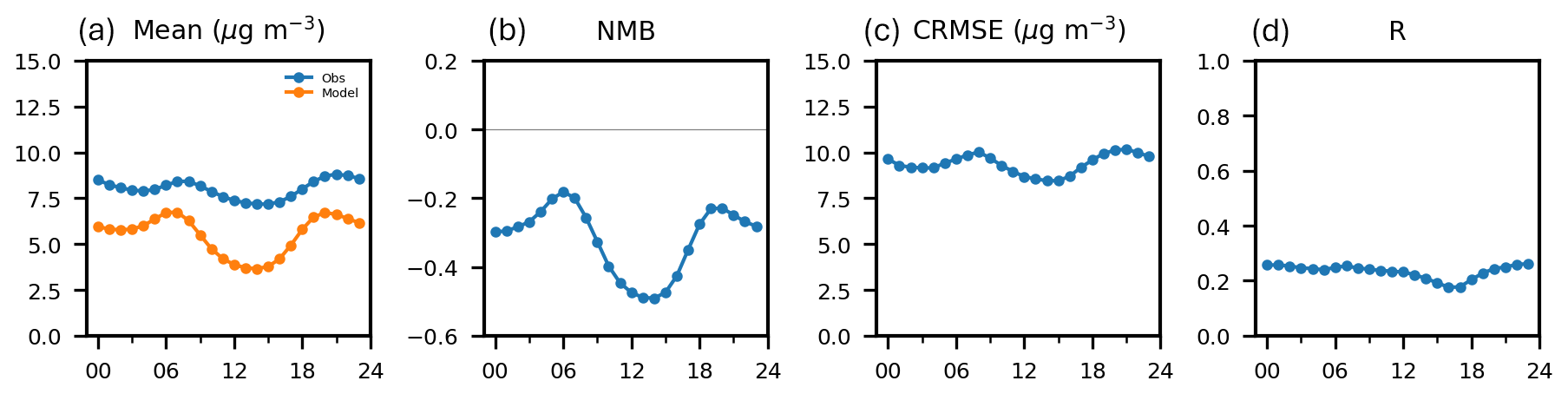
Figure 11Time series of diurnal (a) observed and RAQDPS-OP023-predicted annual-mean hourly PM2.5 concentration (µg m−3) and (b) NMB, (c) CRMSE, and (d) R scores for all of 2021/2022 for all NRT stations. Time is in hours LT.
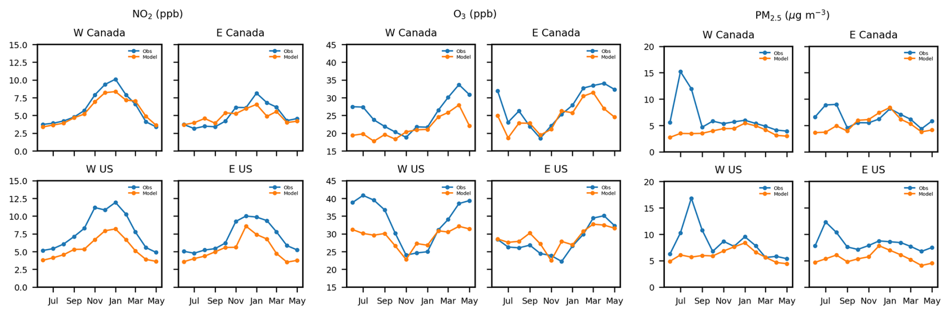
Figure 12Time series of monthly observed and RAQDPS-OP023-predicted annual-mean hourly (left panels) NO2 VMR (ppbv), (centre panels) O3 VMR (ppbv), and (right panels) PM2.5 concentration (µg m−3) for all NRT stations in LT but stratified into four regions (see Fig. S7) for 2021/2022. Orange curves denote predicted monthly values and blue curves denote observed monthly values.
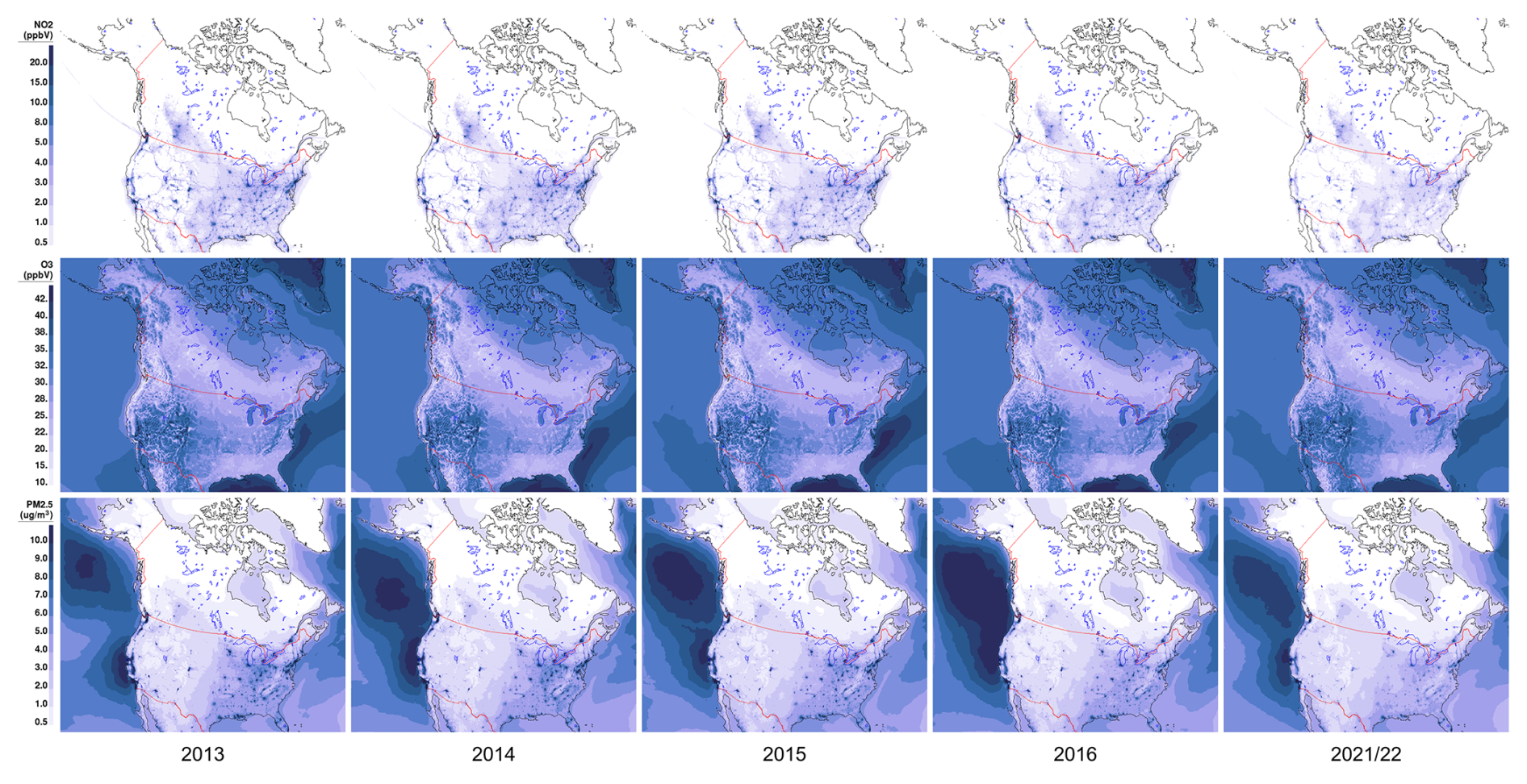
Figure 13Spatial distribution of RAQDPS-OP023-predicted annual-mean abundances of hourly (top row panels) NO2, (middle row panels) O3, and (bottom row panels) PM2.5 total mass for five years (from left to right, 2013–2016 and 2021/2022). Units are ppbv, ppbv, and µg m−3, respectively.
Figure 11 shows all-station annual-mean diurnal time series of five statistics for hourly PM2.5 surface concentration for 2021/2022. RAQDPS-OP023 performance for PM2.5 clearly varied with time of day. Predicted annual-mean hourly concentrations were biased low at all hours of the day, and they displayed more diurnal variability than the measurements. The largest negative annual-mean hourly NMB value occurred in the early afternoon (14:00 LT) while the smallest values occurred at the beginning of the morning rush hour (06:00 LT) and towards the end of the evening rush hour (20:00 LT). Annual-mean hourly CRMSE and R values, on the other hand, exhibited relatively small diurnal variations.
It is also of interest to examine how RAQDPS-OP023 performance varied with geography. Figure 12 compares regional time series of observed and predicted regional monthly means of hourly PM2.5 surface concentration for 2021/2022 for the four continental quadrants (Fig. S7). Peak observed monthly mean PM2.5 concentrations occurred in July or August and were higher in the west than in the east, but as in Fig. 8 there was also a secondary peak in the cold season in December or January for all four regions (cf. Fig. 5). In contrast the predicted monthly mean PM2.5 concentrations had a primary cold-season peak in December or January and a weak warm-season secondary peak in July or August, again consistent with Fig. 8. Note that the RAQDPS-OP023-predicted warm-season peak occurred without any contribution from BB emissions, suggesting a second warm-season emissions source such as biogenic secondary organic aerosol (SOA). Another regional difference is that predicted monthly mean PM2.5 concentrations were higher than the observed values in early winter for eastern Canada but were lower for all months for the other three regions.
2013–2016 hindcasts of PM2.5 total mass
Figure 13 shows the RAQDPS-OP023-predicted spatial distributions of annual mean PM2.5 surface concentration fields (including the sea-salt component) over the model domain for 2013–2016 and 2021/2022. The spatial patterns of annual mean PM2.5 concentration for these five years are broadly similar, although some minor variations between years can be seen over the ocean regions due to variations in sea-salt emissions that result from interannual differences in near-surface wind speed (cf. Fig. S9). Over North America, annual mean PM2.5 surface concentrations, like annual mean NO2 surface VMRs, are highest over the eastern US and California and lower over most of Canada and the rest of the western US, with the exception of isolated urban areas in the western US and a tongue of elevated PM2.5 levels over the Canadian province of Alberta. The impact of the large decreases in domain-total anthropogenic emissions of two PM2.5 precursors, SO2 and NOx, of 60 % and 36 % from 2013 to 2021 (Table 1) is also reflected in this figure by a decrease in PM2.5 levels with time over North America (see also the multi-year plots of annual mean PM2.5-SO4 and PM2.5-NO3 concentration fields in Fig. 14).
Figure 14Spatial distribution of RAQDPS-OP023-predicted annual-mean ambient surface concentrations of nine daily PM2.5 chemical components (µg m−3) for five years (from left to right panels, 2013–2016 and 2021/2022). These components are SO4, NO3, NH4, EC, POM, SOM, TOM, CM, and SS (in rows ordered from top to bottom panels).
Table 3 lists annual values of 12 evaluation statistics for PM2.5 hourly surface predictions for all stations measuring hourly PM2.5 for the 2013–2016 RAQDPS-OP023 hindcasts in addition to the 2021/2022 forecasts. The values of predicted annual mean PM2.5 surface concentrations show a noticeable downward trend across the five simulation years: the observed annual mean surface concentrations also show a downward trend but it is much weaker. This difference might be due in part to the impact of BB emissions of PM2.5 on observed ambient PM2.5 values that is missing from the predicted ambient PM2.5 values. Overall, the 2013–2016 scores for each statistic were very similar amongst themselves, suggesting consistent behaviour in RAQDPS-OP023 PM2.5 predictions from year to year, but some differences are evident between the 2013–2016 scores and the 2021/2022 scores. Annual NMB values were negative for all five years, but the range for 2013–2016 was −0.06 to −0.09, considerably better than the 2021/2022 value of −0.31. Annual NMAE scores, on the other hand, were slightly worse for 2013–2016 (0.71–0.73) than 2021/2022 (0.66), while annual FAC2 scores were slightly better (0.48–0.50 vs. 0.46) and annual R scores were comparable (0.17–0.29 vs. 0.24). Note that all of the annual NMB scores for 2013–2016 (unlike 2021/2022), but none of the NMAE and R scores, met the PM2.5 benchmarks for acceptable performance recommended by Emery et al. (2017).
In addition to hourly continuous PM2.5 total mass concentration measurements, there are also roughly 900 daily PM2.5 monitors operating in North America that make 24-hour PM2.5 total mass measurements using a filter-based, gravimetric approach (see Sect. S2.3 and Table S2c). These daily gravimetric PM2.5 measurements mainly support regulatory and human health applications and are not available in near-real time, but they are notable because they represent an independent data source for model evaluation that can supplement the Class III FEM and non-FRM/FEM hourly continuous PM2.5 concentration measurements used for NRT evaluations and the Table 3 statistics. Daily gravimetric PM2.5 measurements also have different uncertainties than the hourly continuous PM2.5 measurements, including negative artefacts due to the volatilization of semi-volatile species such as ammonium, nitrate, and particle water during transport to and inside the controlled laboratory environments where filter analyses are performed (e.g., Frank, 2006; Dabek-Zlotorzynska et al., 2011; Malm et al., 2011; Chow et al., 2015; Hand et al., 2019). Gravimetric PM2.5 monitor locations from the AQS, IMPROVE, and NAPS networks are shown in Fig. S6a (vs. Fig. S3c for continuous PM2.5 monitors). Note that these combined networks include monitors with every-day, one-day-in-three, and one-day-in-six sampling frequencies, but roughly 65 % of the daily gravimetric PM2.5 mass measurements in the US are made by non-speciation, mass-only monitors (Tables 5 and S2c; Malm et al., 2011).
Table 5 lists all-station annual evaluation statistics for gravimetric measurements of daily PM2.5 mass for the 2013–2016 hindcasts. First, note that observed annual PM2.5 total mass concentration values for the gravimetric data set in Table 5 have a range from 7.2 to 8.2 µg m−3, similar to but smaller than the corresponding range of 7.4 to 8.7 µg m−3 for the hourly continuous PM2.5 data set from Table 3. The range of annual NMB scores for the gravimetric data set, however, is 0.0 to 0.07, slightly better and of opposite sign to the range of −0.09 to −0.06 for the continuous PM2.5measurements in Table 3. Other annual scores for the 2013–2016 hindcasts are also better for the gravimetric measurement data set. The range of annual NMAE scores for the gravimetric PM2.5 measurements is 0.51 to 0.54 (vs. 0.71 to 0.73 for the continuous PM2.5 measurements), the range of annual FAC2 scores is 0.68 to 0.70 (vs. 0.48 to 0.50), and the range of annual R scores is 0.43 to 0.47 (vs. 0.17 to 0.29). Note the narrow range of each of these annual statistics for the four years, suggesting a high level of consistency in model performance. Note too that the range of annual NSD scores for the gravimetric measurements is 1.41 to 1.61, higher than the range of 0.78 to 1.36 for the continuous PM2.5 measurements.
Some differences in scores for these two independent data sets are to be expected due to differences in monitor locations, in temporal aggregation (daily vs. hourly), and in measurement technologies. One reason for some of the better scores for the gravimetric PM2.5 mass measurements may be their daily sampling period, which will reduce the influence of short-term model errors compared to the hourly continuous measurements (e.g., Appel et al., 2008, 2021). The sampling period would not, however, affect annual means or MB and NMB scores. One technical difference between the daily gravimetric PM2.5 mass measurements and the continuous mass measurements is that the filter analysis for the former is performed under constant-temperature, low-humidity conditions in a laboratory after transport from the field and storage prior to analysis whereas the hourly continuous mass measurements are made under ambient conditions where temperature and humidity can vary widely. This means that daily gravimetric PM2.5 mass values are likely to be lower than daily continuous PM2.5 mass values due to loss of some semi-volatile mass from ammonium nitrate, organic matter, or particle water from the sample filter, especially for filters exposed under high-humidity or low-temperature ambient conditions. The fact that annual NMB scores for gravimetric PM2.5 mass measurements are more positive than those for continuous PM2.5 measurements is thus somewhat surprising.
Additional analyses
The results of additional analyses for hourly continuous and daily gravimetric PM2.5 total mass measurements with a focus on the 2013–2016 hindcasts are presented in Sect. S3.2.2. These results include tables of separate annual and seasonal scores for the individual AQS, IMPROVE, and NAPS networks as well as regional scores for all five years, spatial plots of both annual station scores and predicted seasonal mean PM2.5 surface concentration fields for 2013–2016, seasonal and regional diurnal analyses for 2021/2022, and monthly time series, monthly density scatterplots, and urban vs. rural monthly time series for 2013–2016. One insight from these additional analyses are the considerable variations between seasons that are evident across all five years in the seasonal mean PM2.5 mass fields, in the seasonal statistical scores, and in monthly mean time series (e.g., Figs. S13 and S142). Another is the high level of consistency between seasonal scores for PM2.5 for the 2013–2016 hindcasts (and in many cases for the 2021/2022 forecasts) at the aggregated all-station level and annual scores at the individual station level, which allows systematic model errors to be identified. For example, all-station monthly NMB scores were most negative in summer for all four years (Figs. S142 and S198). Third, some of the analyses suggest that the neglect of BB emissions by the RAQDPS-OP023 was an important contributing factor to its overall underpredictions of PM2.5 total mass. Fourth, there were some striking differences for 2013–2016 between the time series of monthly PM2.5 statistics for urban stations (Fig. S213) vs. rural stations (Fig. S214) that underline the importance of emissions forcing. For example, monthly NMB values for the urban stations were positive for some months whereas they were uniformly negative for the rural stations, suggesting that PM2.5 underprediction is mainly a rural issue. Fifth, additional differences are shown between evaluation statistics for 2013–2016 for daily gravimetric PM2.5 total mass measurements vs. hourly continuous PM2.5 measurements. These differences include positive monthly NMB scores for the cold-season months for the gravimetric measurements (Fig. S198) vs. lower scores for the continuous measurements (Fig. S142). And sixth, some of the evaluation scores between individual networks were also very different, and certain differences in the overall characteristics of the individual networks, in particular the dominance of either urban stations or rural stations, can help to explain why the scores between network were different. For example, for the daily gravimetric PM2.5 measurements the seasonal MB and NMB scores for one measurement network (NAPS) were positive for all seasons and for a second network (AQS) they were positive for most seasons (Table S5S). For the hourly continuous PM2.5 measurements, on the other hand, the seasonal MB and NMB scores were negative for both networks for all seasons. The fact that some scores point to model overpredictions of PM2.5 make it clear that the negative all-station MB and NMB scores presented in Table 3 and Figs. 5, 8, and 11 do not tell the whole story. Multiple factors must be considered in addition to model formulation to explain these different scores, including the magnitude and distribution of emissions, seasonal and regional variations in meteorology, differences in network composition, and differences in measurement instrument characteristics.
3.3 Expanded evaluation for additional species and processes
As described in the companion paper by Moran et al. (2026), the RAQDPS023 predicts abundances of 47 individual and lumped gas-phase chemical species and 16 size bin-chemical components. While direct atmospheric measurements are not available for all of these species and components, this section describes evaluation results based on 2013–2016 QA/QCed measurements of nine atmospheric gases in addition to NO2 and O3, seven PM2.5 chemical components, and three aqueous-phase inorganic ions.
3.3.1 Other gases
Table 4 extends the all-station annual statistical scores reported in Table 3 for two gas-phase species, NO2 and O3, to nine other individual or lumped ADOM-2 gas-phase species predicted by the RAQDPS-OP023 for 2013–2016: NO, NOx, HNO3, NH3, SO2, CO, ETHE, HCHO, and ISOP, where ETHE is a lumped species (Sect. S2.4). The measurements considered were provided by five networks: AMoN, AQS, CAPMoN, CASTNET, and NAPS. As discussed in Sect. 2.3 and illustrated by Figs. S4 and S5, the available sets of measurements for these other gas-phase species are different from those for NO2 and O3 in terms of the numbers and the locations of surface monitors, and also, in some cases, the sampling period, which ranged from hourly to biweekly (see also Tables S2a and S2b). Looking at values of N, the number of complete measurements per year, in Table 4, we see that NO, NOx, and CO have the most measurements by far, followed by ETHE and ISOP, then SO2, HCHO and HNO3, and lastly NH3 with the fewest measurements. However, due to the different sampling period lengths, the number of measurements does not necessarily reflect the number of measurement stations. For example, there are more monitors measuring HNO3, NH3, and HCHO than there are measuring ETHE and ISOP (Table S2b) even though N is smaller for the first three species. In fact, only 8 to 13 stations have complete annual measurements for ETHE and only 6 to 13 stations have complete annual measurements for ISOP for 2013–2016. Note that the evaluation scores for HNO3, NH3, and SO2 will also be referred to in the next section, since these three species are precursors to three PM2.5 chemical components.
Table 4Summary table of all-station annual statistics for the RAQDPS-OP023 for nine other ambient gas-phase chemistry measurements (NO, NOx, CO, HNO3, NH3, SO2, ETHE, ISOP, HCHO) for 2013–2016. For dimensional statistics, units are ppmv for CO, µg m−3 for NH3, and ppbv for other species. Sample duration used for all networks is hourly for NO, NOx, CO, ETHE, and ISOP, daily for HCHO, weekly for HNO3 and SO2, and biweekly for NH3.

Table 5Summary table of all-station annual statistics for the RAQDPS-OP023 for daily gravimetric and speciated PM2.5 measurements for 2013–2016. For dimensional statistics, units are µg m−3.
Compared to the annual model performance for NO2 and O3 predictions for 2013–2016 summarized in Table 3, the overall model skill for these other gas-phase species presented in Table 4 is more varied. For example, all-station annual mean NO VMRs, like those for NO2, were overpredicted for all four years (by 9 % to 32 %). All-station annual NMB, NMAE, FAC2, and R scores for hourly NO VMR, however, were less good than those for hourly NO2 VMR for all four years, but this difference is at least partly due to the limited precision at which NO VMR measurements were reported (see Sect. S3.3.1). All-station annual NMB, NMAE, FAC2, and R scores for hourly CO and daily HCHO VMRs, on the other hand, were comparable to those for NO2. All-station annual mean HNO3, SO2, and ISOP VMRs were overpredicted for all four years (and also all months: see Sect. S3.3.1), by 16 % to 33 %, 43 % to 60 %, and 227 % to 271 %, respectively, whereas all-station annual mean NH3 VMR was underpredicted for all four years (and all months: Fig. S145), by 42 % to 47 %. All-station annual mean ETHE was also overpredicted for all four years, by 68 % to 119 %, but these scores were confounded by the inclusion of isoprene oxidation products in addition to ethene in this lumped VOC species (Sect. S2.4), which suggests that overpredictions should be expected. The impact of decreasing SO2 and NOx emissions in 2013–2016 (Table 1) can also be clearly seen in corresponding decreases in Table 4 in both observed and predicted all-station annual mean SO2 and HNO3 VMR values.
Additional analyses
More evaluation results for 2013–2016 for these other gas-phase species are provided in Sect. S3.3.1, including tables of annual and seasonal scores for individual Canadian and US networks as well as all-station regional scores, spatial plots of both annual station scores and predicted seasonal mean surface VMR fields, time series of all-station monthly statistics, and monthly density scatterplots. It is clear from these additional analyses that all nine species exhibit strong seasonal variations: four species (HNO3, NH3, HCHO, ISOP) were observed and predicted to have summer maxima, four (NO, NOx, SO2, CO) were observed and predicted to have winter maxima, and ETHE was observed to have a winter maximum but predicted to have a summer maximum (Table S4S). As noted above, the disagreement for ETHE was not surprising given to the inconsistency between measured ethene and lumped model ETHE. However, winter ETHE scores, when isoprene emissions were low (Table S1), were better than those for the other three seasons, when isoprene emissions were higher (Table S4S). For example, winter NMB values ranged from −6 % to 13 %, suggesting that predictions of pure ethene VMR driven by pure ethene emissions demonstrated skill. As was the case for NO2 and O3, there were also marked similarities in the scores for these other gas-phase species across the four annual hindcast simulations, which supports identification of systematic model errors. For example, SO2 and ISOP were consistently overpredicted and NH3 was consistently underpredicted in all seasons and months (Table S4S; Figs. S146, S150 and S145).
The consistency in annual, seasonal, and monthly scores for the four years also suggests that the year-specific emissions used for these hindcasts were representative. However, some scores discussed in Sect. S3.3.1 raised concerns that Canadian SO2 emissions and biogenic ISOP emissions may have been too high and North American NH3 emissions too low for the 2013–2016 period. The decreases in SO2 and NOx emissions from 2013 to 2016 were also reflected in time series of both observed and predicted monthly mean VMRs for NO, HNO3, and SO2 (Figs. S143, S144 and S146) as well as NO2 (Fig. S140). Performance benchmarks for CO and SO2 proposed by Zhai et al. (2024) are also discussed in Sect. S3.3.1, and more CO scores than SO2 scores met these benchmarks. Scores for individual networks can also be quite different owing to different network characteristics. SO2 provides a good illustration of this behaviour as SO2 measurements were available from four networks: scores for the CAPMoN and CASTNET networks were significantly better overall than those for the AQS and NAPS networks for both annual and seasonal evaluations (Tables S4A and S4S). It was noted that evaluation scores also tended to be similar for species with similar characteristics, such as primary species vs. secondary species and species having similar emissions sources (e.g., combustion). Observed and predicted annual and seasonal CV values for the other gas-phase species were also considered. Based on CV values, they fell naturally into three groups, depending on whether the pollutants were primary, secondary, or mixed primary-secondary in nature. Lastly, it was noted that a few scores for 2016 appeared to be outliers and that monthly density scatterplots for hourly NO and CO revealed obvious precision problems with reported measurements for these two species (Figs. S172 and S176).
3.3.2 PM2.5 chemical composition
As emphasized by Bachmann (2013), PM2.5 is a multi-pollutant. This means that accurate forecasts of PM2.5 total mass require accurate forecasts of its underlying chemical components, each of which has different emissions sources and different formation pathways. Forecast errors for PM2.5 total mass can thus be better understood by examining forecast errors for its underlying chemical components. Fortunately, three North American networks (CSN, IMPROVE, NAPS) make measurements of PM2.5 composition (Sect. 2.3 and Table S2a). Station locations for these three networks are plotted in Fig. S6b, while Table S2c summarizes the number of stations for 2013–2016 for which PM2.5 speciation measurements were available and the smaller number for which temporally representative seasonal and annual measurements were available (see Sect. S2.4).
Figure 14 shows plots of the spatial distributions of annual mean surface concentrations of nine PM2.5 chemical components over North America for 2013–2016 and 2021/2022 predicted by the RAQDPS-OP023. Note that the sets of contour intervals used vary by component, with PM2.5–EC, PM2.5–NH4, and PM2.5–CM having the smallest ranges and PM2.5-SS and PM2.5-TOM (= PM2.5–POM + PM2.5–SOM) having the largest ranges. It is clear from this figure that the predicted spatial distributions vary markedly between PM2.5 chemical components. It is also clear that the predicted annual spatial distributions of each of these chemical components for these five years are broadly similar, pointing to the anchoring effect of relatively constant emissions to the atmosphere of primary PM2.5 chemical components and PM2.5 gas-phase precursors (e.g., Fig. S1), which for most pollutants changed relatively little from year to year (Table 1). The annual mean surface concentrations of PM2.5 total mass shown in Fig. 13 were also broadly similar from year to year. However, a comparison of the spatial distributions of annual mean PM2.5–SO4 and PM2.5–NO3 surface concentrations from 2013 to 2021/2022 in Fig. 14 does suggest decreasing concentrations of these two chemical components over this period, consistent with the large decreases in domain-total anthropogenic emissions of SO2 and NOx from 2013 to 2021/2022 (Table 1). Interestingly, annual mean PM2.5–NH4 surface concentration fields can also be seen to decrease from 2013 to 2021/2022 despite nearly constant NH3 emissions over this period. This downward trend is due instead to the reduced availability of gaseous H2SO4 and HNO3 in the atmosphere, which form sulfate and nitrate particulate salts with NH3. Domain-wide primary PM2.5 emissions also decreased by 8 % from 2013 to 2016 (Table 1), and some decline is evident from 2013 to 2016 for PM2.5-EC and PM2.5-POM in Fig. 14. The annual mean spatial distributions of other PM2.5 components display only small year-to-year variations with the exception of sea salt, for which interannual variations in mean surface concentration are driven by interannual variations in surface wind speed (see Fig. S9).
Although the above discussion suggests the close connection between the spatial distributions of emissions of primary PM2.5 components and PM2.5 gas-phase precursors and the resulting spatial distributions of PM2.5 chemical components in the atmosphere, it is not a simple relationship since many chemical and physical processes in the atmosphere modulate the chemical transformation and removal pathways of these multiple chemical components. For example, the annual spatial distributions of PM2.5–SO4 shown in Fig. 14 are quite smooth, which reflect its origin as a secondary pollutant resulting from gas-phase or aqueous-phase oxidation of North American SO2 emissions, even though the SO2 emissions shown in Fig. S1d are largely emitted by isolated point sources (e.g., ECCC, 2018; Foley et al., 2023). The spatial distribution in Fig. 14 of PM2.5–SOM, another secondary pollutant, is also smooth, but its maximum is located further south over the southeastern US, where biogenic VOC emissions are high, especially in the summer season (cf. Fig. S27). It is also clear from Fig. S1 that there are marked differences in the spatial distributions of some of the anthropogenic emissions associated with different PM2.5 chemical components. For example, the majority of NOx emissions are located in the eastern half of North America, but the locations of some major highways and large urban areas in western North America are visible in the PM2.5–NO3 surface concentration panels in Fig. 14, which suggests the important contributions of on-road mobile sources and population centres to NOx emissions. Emissions of primary PM2.5 and of NH3 gas, the precursor to PM2.5–NH4, on the other hand, are stronger over the North American interior (Fig. S1e and f). Elevated NH3 emissions from agricultural activities in the midwestern US are visible in Fig. S1e as well as fertilizer application in the San Joaquin Valley of California, large animal feedlot operations in Texas and Oklahoma, and extensive swine production in North Carolina. While NH3 emissions are dominated by agricultural activities, some NH3 emissions are also associated with population centres due to on-road mobile emissions (e.g., Toro et al., 2024). In addition, the chemical composition of primary PM2.5 emissions depends on the emissions source type. Combustion sources dominate PM2.5–EC and PM2.5–POM emissions, as suggested in Fig. 14 by their association with major highways and population centres, while the PM2.5-TOM surface concentration field displays characteristics of both the PM2.5–POM and PM2.5–SOM fields. Fugitive dust emissions from paved and unpaved roads are the main source of PM2.5–CM, and PM2.5–CM surface concentrations can be seen in Fig. 14 to be elevated in both urban centres and rural areas. Lastly, the spatial distribution of PM2.5–SS is dominated by its oceanic sources, but the limited transport of sea salt from the oceans inland over most of North America that is evident in Fig. 14 should also be noted.
Table 5 presents all-station annual scores for seven PM2.5 chemical components for 2013–2016 for the three PM2.5 speciation networks combined. The scores for each component tend to be similar from year to year, but scores can also vary considerably between components. For example, all-station annual NMB scores for PM2.5–SO4 and PM2.5–NO3 were negative for all four years whereas all-station annual NMB scores for PM2.5–NH4, EC, CM, and SS were positive for all four years. Only PM2.5-TOM had small all-station annual NMB values of both signs for this period. Note that the PM2.5-NH4 overpredictions are inconsistent with the underpredictions of both PM2.5–SO4 and PM2.5–NO3 given the inorganic salts formed by these three components. One possible explanation is that this is an artefact due to the lack of available IMPROVE PM2.5–NH4 measurements (e.g., Solomon et al., 2014) so that only CSN and NAPS measurements were considered for PM2.5–NH4 in Table 5. However, the same inconsistency can be seen in Table S5A for just CSN measurements. Another possible explanation is that the RAQDPS-OP023 does not consider the neutralization of PM2.5–SO4 and PM2.5–NO3 by base cations, which would reduce PM2.5–NH4 concentrations and increase NH3 VMR (e.g., Vasilakos et al., 2018; Miller et al., 2024; Semeniuk et al., 2025). All-station annual NMAE scores in Table 5 for 2013–2016 were lowest for PM2.5–SO4 (∼0.47), followed in ascending order by annual NMAE scores for PM2.5–NO3, TOM, EC, NH4, CM, and SS (∼1.45). All-station annual FAC2 scores were highest for PM2.5–SO4 (∼0.64), followed in descending order by those for PM2.5–EC, TOM, NH4, NO3, SS, and CM (∼0.31). All-station annual R scores were also highest for PM2.5–SO4 (∼0.66), followed in descending order by those for PM2.5–NO3, EC and SS, NH4, TOM, and CM (∼0.17). Based on the annual NMAE, FAC2, and R scores taken together, the RAQDPS-OP023 showed the most skill for PM2.5–SO4 followed in descending order by PM2.5–NO3, EC, TOM, NH4, SS, and CM.
Note also that all-station annual NSD scores fell into two groups: values for PM2.5–SO4, NO3, and NH4 were less than 1.0 whereas values for PM2.5–EC, TOM, CM, and SS were greater than 1.0. The three components in the first group are all secondary components whereas those in the second group are all primary components or a mixed primary-secondary component in the case of PM2.5–TOM. While this difference might appear to suggest that the model is overemphasizing the contribution of temporal variations due to emissions, the PM2.5 speciation measurements are 24 h samples so that the observed and predicted temporal variation at measurement locations can only be due to interday and longer variations. For anthropogenic emissions this would point to the day-of-week and month-of-year temporal profiles that have been assumed by the emissions processing system for different source sectors (Sect. S2.2), but emissions for the two primary components that had the largest NSD values, PM2.5–CM and SS, are also the ones most affected by meteorology.
It is worth noting that downward trends can be seen in Table 5 in the values of both observed and predicted annual mean concentrations for PM2.5–SO4, NO3, and NH4, consistent with the monotonic decreases in SO2 and NOx emissions that occurred over this period and with Fig. 14. For the PM2.5–SO4 evaluation statistics, the values of annual RMSE and R also decreased from 2013 to 2016. This is similar to decreases in these two statistics reported by Kelly et al. (2019) for the CMAQ model over the 2007 to 2015 period, which they attributed to decreasing SO2 emissions and lower summertime PM2.5–SO4 peaks, which in turn reduced the PM2.5–SO4 “signal” (e.g., Chan et al., 2018). Note also that 2016 annual , , MB, NMB, RMSE, R, σO, and σM scores for PM2.5–SO4, NO3, EC, and OC for two recent versions of the CMAQ model (with wildfire emissions) were reported in Appel et al. (2021). Although minor methodological differences such as inclusion or exclusion of NAPS measurements are suggested by comparisons of the 2016 and σO scores in Table 5 and in Appel et al. (2021), there is rough agreement between the 2016 RAQDPS-OP023 scores and CMAQ scores for PM2.5–SO4, NO3, and EC while RAQDPS-OP023 PM2.5–TOM scores cannot be compared directly with CMAQ PM2.5–OC scores.
PM2.5 reconstructed mass
PM2.5 speciation measurements can also be used to calculate PM2.5 reconstructed dry mass (i.e., excluding aerosol water) as a weighted sum of the individual PM2.5 chemical components (e.g., Malm et al., 2011; Chow et al. 2015; Hand et al., 2019). This is often done with the IMPROVE formula, which uses some measured components directly and some measured components as proxies for the TOM, CM, and SS components, which are not measured directly. The RAQDPS-OP023 PM2.5 total mass forecasts, on the other hand, which are the sum of the seven predicted PM2.5 chemical components shown in Table 5 (including SS but excluding aerosol water), are thus also a reconstructed dry mass but do not require the use of any proxies. A slightly modified version of the IMPROVE formula has been used in this study to calculate PM2.5 reconstructed mass from speciation measurements (see Sect. S3.3.2 for more details).
Figure 15 compares observed and RAQDPS-OP023-predicted all-station seasonal mean PM2.5 reconstructed dry mass and chemical composition for 2013–2016 based on combined CSN, IMPROVE, and NAPS measurements that were mass-complete (Sect. S3.3.2). There is good agreement overall between the seasonal means of observed and predicted PM2.5 reconstructed dry mass. Predicted PM2.5 total mass was greater than observed PM2.5 reconstructed total mass for all four winters, while the opposite was true for all four summers, with closer agreement for spring and autumn. This good agreement might seem surprising given the consistent model underpredictions of hourly PM2.5 mass measurements described in Sect. 3.2.2, but it is more consistent with the better evaluation results for daily gravimetric PM2.5 mass measurements also discussed in that section. Similar comparisons for the CMAQ model against CSN and IMPROVE measurements have been presented for 2011 and 2016 simulations by Appel et al. (2017, 2021). Interestingly, both models overpredicted PM2.5 total mass in winter 2016 and underpredicted it in summer 2016.
Figure 15Stacked bar graphs of observed vs. RAQDPS-OP023-predicted domain-wide season-mean PM2.5 chemical component concentrations (µg m−3) based on combined CSN, IMPROVE, and NAPS PM2.5 speciation daily measurements and hindcasts for four consecutive years. The top row corresponds to 2013 seasons, the next two rows below to 2014 and 2015 seasons, and the bottom row to 2016 seasons. Each row has four seasonal bar-graph pairs (observed and predicted), starting with winter (DJF) on the left, and then spring (MAM), summer (JJA), and autumn (SON) on the right. The stars mark the measured or predicted season-mean gravimetric PM2.5 total mass.
In addition, the stars plotted in Fig. 15 indicate the seasonal means of observed gravimetric PM2.5 total mass for 2013–2016. It is natural to compare gravimetric PM2.5 total mass and PM2.5 reconstructed mass since they both attempt to measure of the same quantity. Good agreement can be seen in the observations between these two measurements for three seasons but not for the summer, for which the gravimetric total mass was larger. This is consistent with previous findings by Malm et al. (2011) for the CSN and IMPROVE networks. Predicted seasonal means of PM2.5 total mass, on the other hand, were greater than the gravimetric seasonal means in winter and autumn but were even smaller than the observed PM2.5 reconstructed mass in summer. A closely related quantity, the PM2.5 residual mass, is defined to be the difference between gravimetric PM2.5 mass and reconstructed PM2.5 mass (e.g., Hand et al., 2019). Observed seasonal mean PM2.5 residual mass was greater than 0.5 µg m−3 for summer but was small otherwise, whereas predicted seasonal mean PM2.5 residual mass was greater than 1 µg m−3 for summer but was negative for winter, with values ranging from −1.47 to −0.90 µg m−3 (see Table S5S-mr). Hand et al. (2019) found observed seasonal PM2.5 residual mass to be mostly positive after 2011 with a strong summer peak, consistent with Fig. 15. Given the marked RAQDPS-OP023 underpredictions of summer mean gravimetric PM2.5 total mass but overpredictions of winter mean gravimetric PM2.5 total mass (Sect. S3.2.2), the factors that contribute to the non-negligible observed summer PM2.5 residual mass may be of interest because they may also be relevant to the model performance. Malm et al. (2011), Chow et al. (2015), and Hand et al. (2019) have suggested that some of these factors may be the neglect of particle-bound water in calculating PM2.5 reconstructed mass, ammonium and nitrate volatilization under laboratory conditions, and seasonal variations (lower in winter, higher in summer) in the OM : C scaling ratio needed to scale observed OC concentration to ambient TOM concentration. Note too that the volatilization of PM2.5–NO3 and PM2.5–NH4 during the transport, storage, and analysis of filter samples, a negative measurement artefact, will create spurious positive model biases for these two PM2.5 components (cf. Table 5).
Figure 15 also shows good agreement overall between observed and RAQDPS-OP023-predicted seasonal mean PM2.5 chemical composition. Looking component by component, the dominant contribution of the PM2.5–EC and TOM carbonaceous components to PM2.5 total mass is evident in both the observed and predicted stacked bar graphs as are the anticorrelated seasonal variations in PM2.5–SO4 and PM2.5–NO3. Overpredictions of PM2.5-TOM concentration in the winter but underpredictions in the summer can be seen for all four years. The decrease in the observed and predicted contribution of the three major inorganic ions (SO4, NO3, NH4) to PM2.5 total mass from 2013 to 2016 due to decreases in annual SO2 and NOx emissions can also be seen. Some of the annual mean biases for the PM2.5 chemical components noted in Table 5 are also reflected in almost all seasons in Fig. 15, including the underpredictions of PM2.5–SO4 and NO3 and overpredictions of PM2.5–EC and SS. In fact, the reduction of bias for predictions of PM2.5 total mass that is associated with the summation of these components, with their individual underpredictions and overpredictions is an example of the positive impact that compensating errors can have on model skill, and it demonstrates the value of a more comprehensive evaluation of model performance, in this case evaluating the prediction of PM2.5 chemical components in addition to PM2.5 total mass.
Figure 16Time series of RAQDPS-OP023-predicted monthly mean variation of eight daily PM2.5 chemical component concentrations (µg m−3) area-weighted averaged over North American continent grid cells and 2013 to 2016 simulations. These components are SO4, NO3, NH4, EC, POM, SOM, CM, and SS (shown ordered from bottom to top in stacked bar graphs).
Since Fig. 15 is based on measurements from sampling sites located mainly over the continental US (see Fig. S6b), it does not account for PM2.5 composition over northern Mexico and most of Canada. Figure 16, by contrast, shows a monthly time series of the RAQDPS-OP023-predicted mean PM2.5 chemical composition averaged over the land portion of the domain and the 2013–2016 simulations, with PM2.5–TOM separated into POM and SOM (not possible for the measurements). Seasonal variations of PM2.5–SO4, NO3, POM, SOM, and SS can be clearly seen, whereas seasonal variations of PM2.5–NH4, EC, and CM are less pronounced. PM2.5–NO3 and POM are predicted to have winter maxima and summer minima, whereas PM2.5–SO4 and SOM are predicted to have winter minima and summer maxima. Note that the total inorganic component (sum of PM2.5–SO4, NO3, and NH4) only has a relatively small monthly variation with a minimum in November. The predicted peak monthly mean PM2.5 total dry mass occurs in August, driven by monthly maximum values of PM2.5–SO4 and SOM. This is different from Figs. 8 and 15, where the highest PM2.5 total mass was predicted to occur in the winter, but note that predicted PM2.5 total mass in Figs. 8 and 15 is roughly 6 µg m−3 vs. 1.5 µg m−3 in Fig. 16, which suggests that the former overweight the influence of urban areas. One other interesting feature in Fig. 16 is the SS maximum in August, which is in apparent contradiction to the SS intertime maximum evident in Fig. S30. However, while Fig. S30 showed that inland penetration of sea salt over North America is limited, some seasonal variations are evident near California, the US Gulf coast, and Florida that may be associated with the occurrence of sea-land breezes in the warm season (and observed seasonal-mean SS values in Table S5S are largest in the spring and summer). Lastly, Fig. S203 presents a similar analysis to Fig. 16 but for averaging over the full domain. Unlike Fig. 16 the SS component clearly dominates PM2.5 total dry mass in this figure, reflecting predicted high levels of sea salt over the Pacific and Atlantic Oceans. In addition, the largest monthly mean SS concentrations in Fig. S203 occur in the cold season, consistent with Fig. S30.
Figure 17Time series of RAQDPS-OP023-predicted season-mean diurnal (UTC) variation of eight hourly PM2.5 chemical component concentrations (µg m−3) area-weighted averaged over North American continent grid cells and 2013 to 2016 simulations for each of four seasons: (a) winter; (b) spring; (c) summer; and (d) autumn. These components are SO4, NO3, NH4, EC, POM, SOM, CM, and SS (shown ordered from bottom to top in stacked bar graphs).
It is also informative to look at the diurnal variation of the PM2.5 chemical components. Figure 17 shows the predicted diurnal variation of eight PM2.5 chemical components for each season after averaging over the 2013–2016 simulations and all North American continental grid cells. It is clear from this figure that both PM2.5 total mass and chemical composition are predicted to vary with time of day. PM2.5 total mass has a maximum for three seasons at 12:00 UTC (= 07:00 EST), near sunrise and morning rush hour, and a minimum in all seasons at 21:00 UTC (= 16:00 EST). The wintertime maximum, on the other hand, occurs at 04:00 UTC (i.e., near local midnight), pointing to a different balance between surface emissions and vertical stability and mixing. Note too that the individual PM2.5 chemical components display different diurnal behaviours. Hourly PM2.5–SO4 concentration is predicted to be effectively constant, consistent with a nonvolatile secondary pollutant. Hourly PM2.5–NO3 and NH4 concentrations, by contrast, are lowest in the afternoon when near-surface temperature is highest, and highest at night, especially before sunrise when near-surface temperature is often lowest. This behaviour is consistent with the semi-volatile nature of ammonium nitrate, for which lower temperatures favour the particle phase (e.g., Malm et al., 2004; Yu et al., 2005). Hourly PM2.5–EC, POM, and CM concentrations are also predicted to be highest during the night and lowest in the afternoon, but this behaviou is likely due to greater vertical mixing of local emissions during the day, which reduces the near-surface buildup of these three primary species. Hourly PM2.5–SOM, which is assumed to be nonvolatile in the RAQDPS-OP023 (see companion paper by Moran et al., 2026), behaves like PM2.5–SO4 and displays little diurnal variation. Finally, sea-salt concentrations tend to be higher at night and lower during the day, likely due to diurnal variations in surface wind speed and hence in sea-salt emissions.
Note that the daily measurements made by the PM2.5 speciation networks are not able to confirm the diurnal variations of PM2.5 chemical components in Fig. 17 predicted by the RAQDPS-OP023. However, the all-station, annual-mean diurnal analyses of observed and predicted hourly PM2.5 total mass shown in Fig. 11 for North America for 2021/2022, in Fig. S167 for four seasons, and in Fig. S168 for four sub-continental regions, all suggest that measured diurnal variations were smaller than the predicted variations. Two contributing factors to this difference might be the diurnal allocation of primary PM2.5 emissions used by the RAQDPS-OP023 and the parameterization of PM2.5 chemical volatility, including ammonium, nitrate, and water components. Interestingly, Fig. S167 shows that the observed diurnal variation was largest in the winter and smallest in the summer, which is consistent with Fig. 17. In addition, both the observed and predicted all-station, seasonal-mean diurnal curves of PM2.5 total mass in Fig. S167 have one peak at about the time of morning rush hour and sunrise and a second peak at about the time of evening rush hour and sunset. By contrast the seasonal continent-wide diurnal time series in Fig. 17 only have one peak, in the morning near sunrise, but the majority of grid cells sampled for this figure will contain little vehicular activity, unlike the urban areas in which many monitors are located.
Additional analyses
More evaluation results for the daily PM2.5 speciation measurements and gravimetric PM2.5 total mass measurements for 2013–2016 can be found in Sect. S3.3.2. These results include tables of annual and seasonal scores for the individual CSN, IMPROVE, and NAPS networks as well as regional scores, spatial plots of annual MB, NMB, CRMSE, and R station scores for each PM2.5 chemical component, spatial plots of predicted seasonal mean PM2.5 component concentration fields (cf. Fig. 14), monthly time series of PM2.5 component statistics, monthly density scatterplots, and additional stacked bar graphs stratified by network and by region. The discussion of Table 5 noted consistent annual underpredictions or overpredictions for some of the seven PM2.5 chemical components for the 2013–2016 hindcasts. Similarly consistent biases were found throughout the year by season or month for the combined networks for three PM2.5 components, namely underpredictions for PM2.5–SO4 (Fig. S151) and overpredictions for PM2.5–EC (Fig. S154) and PM2.5-SS (Fig. S157). In addition, PM2.5–TOM, the component found to have the smallest annual NMB values, was shown to have pronounced seasonal biases consistent with Fig. 15, with marked overpredictions in winter and underpredictions in summer (Fig. S155). Nevertheless, performance benchmarks for five PM2.5 chemical components (SO4, NO3, NH4, EC, TOM) proposed by Emery et al. 2017) were also compared with both annual and seasonal scores. Nearly all PM2.5-SO4, NO3, NH4, and TOM annual NMB scores and many seasonal scores met acceptable NMB benchmarks, all PM2.5–SO4 and NO3 annual and most seasonal NMAE scores met acceptable NMAE benchmarks, and all PM2.5–SO4, NO3, NH4, and EC annual and seasonal R scores met acceptable R benchmarks. Some annual and seasonal biases were also shown to be network-dependent. Annual NMB values for 2013–2016 for PM2.5-TOM ranged from 0.20 to 0.31 for CSN and from 0.52 to 0.80 for NAPS vs. −0.46 to −0.30 for IMPROVE (Table S5A). For PM2.5–CM the network-dependent biases were even more pronounced: annual NMB values ranged from 1.23 to 1.59 for CSN and from 1.96 to 2.34 for NAPS vs. −0.59 to −0.50 for IMPROVE. Seasonal PM2.5–SO4 was underpredicted and PM2.5–SS was overpredicted throughout the year for all three speciation networks, but PM2.5–EC was overpredicted for the urban-focused CSN and NAPS networks in all seasons but not for the rural-focused IMPROVE network (Table S5S). Since PM2.5–EC, POM, and CM are all primary pollutants, some of these model biases might be connected to the representation of primary PM2.5 emissions.
The systematic biases by network that were identified for some PM2.5 chemical components also affect predictions of PM2.5 composition and total mass. The discussion of Fig. 15 noted that the best agreement was for spring and autumn. However, when the same analysis was applied to only CSN measurements and to only IMPROVE measurements, the agreement was less good for these two seasons, with the RAQDPS-OP023 overpredicting PM2.5 total mass for CSN for spring and autumn (Fig. S200) and underpredicting PM2.5 total mass for IMPROVE (Fig. S201). The findings were similar for a regional analysis, where predicted PM2.5 composition and total mass were in very good agreement with the combined measurements for the WUS and EUS (Fig. S205), but the same regional analysis for CSN-only measurements (Fig. S206) and IMPROVE-only measurements (Fig. S207) revealed errors of opposite sign, with overpredictions of PM2.5 total mass for CSN for the WUS and underpredictions of PM2.5 total mass for IMPROVE for both the WUS and EUS. The presence of these compensating errors for urban-focused and rural-focused stations again points to the benefits of performing a more disaggregated analysis. These network-dependent differences are also consistent with the finding in Sect. 3.2.2 that underprediction of PM2.5 total mass by the RAQDPS-OP023 appears to be mainly a rural issue. Predicted peak seasonal concentrations for PM2.5-NO3, NH4, POM, and SS occurred in the winter (Figs. S23, S24, S26 and S30) vs. summer peaks for PM2.5–SO4, SOM, and TOM (Figs. S22, S27 and S28). This seasonal phase shift can help to explain the bimodality that was observed in monthly PM2.5 total mass (Figs. 8 and S198).
Additional close links were also evident between the inorganic PM2.5 components and their gas-phase precursors. For example, the monthly mean concentration time series for PM2.5–SO4 (Fig. S151) was seasonally anticorrelated with the monthly time series for its gas-phase precursor SO2 (Fig. S146): that is, the PM2.5–SO4 time series had an observed and predicted summer maximum and winter minimum and monthly NMB values were negative, while the SO2 time series had an observed and predicted winter maximum and summer minimum and monthly NMB values were positive. The monthly mean concentration time series for PM2.5–NO3 (Fig. S152) was seasonally anti-correlated with that for its gas-phase precursor HNO3 (Fig. S144) (and also PM2.5–SO4): that is, the PM2.5–NO3 time series had an observed and predicted summer minimum and winter maximum and was mostly underpredicted while the HNO3 time series had an observed and predicted winter minimum and summer maximum and was overpredicted. The monthly mean concentration time series for PM2.5–NH4, the third inorganic component (Fig. S153), was also seasonally anticorrelated with that for its gas-phase precursor NH3 (Fig. S145) (and also HNO3): that is, the PM2.5–NH4 time series had an observed and predicted summer minimum and winter maximum and was mostly overpredicted while the NH3 time series had an observed and predicted winter minimum and summer maximum and was underpredicted. Lastly, downward time trends for 2013–2016 were also visible in observed monthly surface concentrations of PM2.5-SO4 and NH4 (Figs. S151 and S153) due to the SO2 and NOx emissions decreases that took place over this period.
3.3.3 Precipitation chemistry
Precipitation-chemistry measurements are valuable for model evaluation because they are quite different from the air-chemistry measurements considered in the previous sections. One difference is that they quantify a removal process, wet deposition, as opposed to near-surface ambient concentrations determined by dispersion and chemistry. In addition, they represent removal through a column extending from the Earth's surface to cloud top rather than a pure surface-level quantity. They are also an integrated measurement in terms of both gas-particle partitioning and aerosol particle size distribution because they can include contributions from both gas and particle phases and from all aerosol particle sizes. Precipitation-chemistry measurements can thus provide some important insights into removal processes and atmospheric mass budgets for sulfur, oxidized nitrogen, reduced nitrogen, and base cations. As described in Sect. 2.3, two large national networks are responsible for North American precipitation-chemistry measurements, CAPMoN in Canada and NADP in the US.
Figure 18Spatial distribution of RAQDPS-OP023-predicted annual-mean concentrations in precipitation (mg L−1) of (top row panels) SO, (middle row panels) NO, and (bottom row panels) NH for five years (from left to right, 2013–2016 and 2021/2022).
Figure 18 shows the RAQDPS-OP023-predicted spatial distributions of annual mean concentration in precipitation over North America of the three major inorganic ions, SO, NO, and NH, for 2013–2016 and 2021/2022. Several features are evident. First, the spatial distributions are different for each of these ions, largely in response to the different spatial distributions of their respective precursor emissions (cf. Fig. S1). Annual mean SO concentration in precipitation tends to be larger over the eastern US, whereas annual mean NO and NH concentrations in precipitation are larger over the western and central US. Another feature is that predicted SO and NO annual mean concentrations in precipitation appear to decrease from 2013 to 2021/202, consistent with the 60 % and 36 % decreases in North American SO2 and NOx anthropogenic emissions, respectively, over this period (Table 1). No time trend is evident for this period, however, for annual mean NH concentration in precipitation, which differs from the downward trend for annual mean PM2.5-NH4 concentration visible in Table 5 and Fig. 14. Two reasons are that annual NH3 emissions only decreased slightly (6 %) from 2013 to 2021/2022 and both NH3 and PM–NH4 are removed by precipitation scavenging regardless of the exact balance for gas-particle partitioning, whereas annual mean NH3 VMR displayed a slight upward trend from 2013 to 2021/2022 (cf. Table 4, Fig. S16). Figure 18 also agrees qualitatively with comparable plots of observed annual mean SO, NO, and NH concentrations in precipitation for these four years produced by the US NADP network (e.g., National Atmospheric Deposition Program, 2014, 2017), except for the elevated values of annual mean NO and NH concentrations in precipitation predicted over California in 2013. Note that the corresponding annual wet deposition fields predicted by the RAQDPS-OP023 for 2014–2016 (see Figs. S34–S36) have also been used in a study by Cathcart et al. (2025) to calculate total deposition and acidity and nutrient nitrogen critical-load exceedance fields for Canada.
Table 6Summary table of all-station annual statistics for the RAQDPS-OP023 for weekly precipitation-chemistry measurements for 2013–2016. For dimensional statistics, units are mg L−1 for concentration in precipitation, mm per week for precipitation, and mg m−2 per week for wet deposition. Note that daily CAPMoN measurements have been aggregated to weekly values for consistency with NADP measurements.
Table 6 lists all-station annual evaluation statistics for 2013–2016 for RAQDPS-OP023-predicted weekly concentrations in precipitation of SO, NO, and NH, for weekly precipitation, and for the corresponding predicted weekly wet deposition of these ions. The weekly precipitation scores were already discussed in Sect. 3.1. The reductions in concentration in precipitation of SO and NO from 2013 to 2016 suggested visually by Fig. 18 are confirmed by Table 6. Observed and predicted annual-mean SO weekly concentration in precipitation for the combined networks decreased from 0.81 to 0.62 mg L−1 and from 0.82 to 0.61 mg L−1, respectively, over this period, while observed and predicted annual-mean SO weekly wet deposition decreased from 15.6 to 10.7 mg m−2 per week and from 15.9 to 10.1 mg m−2 per week, respectively. Observed and predicted annual-mean NO weekly concentration in precipitation and weekly wet deposition also declined from 2013 to 2016, though by smaller percentages, from 0.96 to 0.90 mg L−1 and 0.94 to 0.78 mg L−1 and from 16.5 to 14.1 mg m−2 per week−1 and 16.2 to 11.6 mg m−2 per week−1, respectively. By contrast, observed and predicted annual-mean NH weekly concentration in precipitation increased slightly while observed and predicted annual-mean NH weekly wet deposition decreased slightly.
Table 6 also reveals that model performance can vary considerably by ionic species. For example, all-station annual NMB values for SO and NO weekly concentrations in precipitation ranged from −0.01 to 0.14 and from −0.14 to −0.01, respectively, but corresponding all-station annual NMB values for NH weekly concentration in precipitation ranged from 0.23 to 0.41, pointing to a considerable and consistent overprediction for this quantity. All-station annual NMB scores for SO, NO, and NH weekly wet deposition ranged from −0.06 to 0.05, −0.18 to −0.02, and 0.13 to 0.16, respectively, suggesting small biases for SO wet deposition, a small but consistent underprediction for NO wet deposition, and a consistent overprediction for NH wet deposition. In comparison, Simon et al. (2012) reported (25 %, 75 %) quantile values for NMB scores for accumulated seasonal and annual SO, NO, and NH wet deposition of (−0.01, 0.23), (−0.37, 0.10), and (−0.21, 0.0), respectively, in a review of North American AQ model performance evaluations. The RAQDPS-OP023 annual NMB scores fit comfortably with these reported ranges. Zhang et al. (2018c) reported mean NMB values for SO, NO, and NH accumulated annual wet deposition of −0.05, −0.32, and −0.31, respectively, for the 1990–2010 period using the CMAQ model without post-processing adjustments, and Benish et al. (2022) obtained mean NMB values for SO, NO, and NH accumulated annual wet deposition of −0.12, −0.10, and −0.20 for the 2002–2017 period using a newer version of the CMAQ model but also without post-processing adjustments. Note that the negative bias in NO concentration in precipitation and wet deposition is consistent with the neglect of lightning NO emissions in both CMAQ and the RAQDPS-OP023 (Zhang et al., 2018c).
Corresponding all-station annual NMAE values from Table 6 for SO, NO, and NH weekly concentrations in precipitation for 2013–2016 ranged from 0.59 to 0.68, 0.52 to 0.57, and 0.78 to 0.95, respectively, and annual NMAE values for SO, NO, and NH weekly wet deposition ranged from 0.61 to 0.65, 0.52 to 0.55, and 0.68 to 0.72. The NMAE scores for weekly wet deposition compare favourably with top-quartile NMAE scores for monthly SO, NO, and NH wet deposition of 0.61, 0.51, and 0.57 compiled by Simon et al. (2012) despite their lower level of temporal aggregation. All-station annual FAC2 values for weekly concentration in precipitation were slightly higher (better) for NO (0.68–0.70) than for SO or NH (0.63–0.65; 0.57–0.60), and the same was true for weekly wet deposition (0.62–0.64 vs. 0.53–0.56 and 0.55–0.57). All-station annual R scores for all stations were also slightly higher for NO weekly concentration in precipitation (0.46–0.52) than for SO or NH weekly concentration in precipitation (0.25–0.41, 0.38–0.47), whereas all-station annual R scores for SO, NO, and NH weekly wet deposition were comparable (0.49–0.58, 0.46–0.59, 0.47–0.59). By comparison, Zhang et al. (2018c) obtained higher mean R scores for accumulated SO, NO, and NH annual wet deposition for the 1990-2010 period of 0.92, 0.89, and 0.77, respectively, and Benish et al. (2022) obtained mean R scores for accumulated SO, NO, and NH annual wet deposition for the 2002–2017 period of 0.78, 0.77, and 0.61, but these higher scores may again be explained at least in part by the much greater temporal aggregation and averaging. Note also that the values of the statistics in Table 6 were fairly constant across the four years in spite of the large SO2 and NOx emission reductions, again suggesting that the year-specific input emissions that were used for the retrospective simulations were representative of each year.
Additional analyses
More evaluation results for predicted SO, NO, and NH weekly concentrations in precipitation and weekly wet deposition can be found in Sect. S3.3.3. These include tables of separate annual and seasonal scores for the CAPMoN and NADP networks for 2013–2016 as well as regional scores, spatial plots of annual MB, NMB, CRMSE, and R scores at individual stations, spatial plots of predicted seasonal concentration in precipitation and wet deposition fields for 2013–2016 and 2021/2022, monthly time series of statistics for weekly concentrations in precipitation and wet deposition, and monthly density scatterplots. A number of additional insights can be found in these supplemental analyses. For example, the separate annual and seasonal scores for the CAPMoN and NADP networks presented in Tables S6A and S6S revealed that RAQDPS-OP023 scores were better overall for CAPMoN than NADP. For example, annual R scores were consistently higher for CAPMoN than NADP for SO, NO, and NH weekly concentrations in precipitation and weekly wet deposition. Some regional differences were also evident in many of the spatial distributions of station-specific annual values of MB, NMB, CRMSE, and R. For example, the station-level annual MB scores for SO weekly concentration in precipitation tended to be positive in eastern Canada and the northeastern US but negative elsewhere (Fig. S109). Annual R values for SO and NO weekly wet deposition also tended to be lower in the west and higher in the east (Figs. S128 and S132). It is also clear from Table S6S and Figs. S158–S164 that seasonal model skill was consistent overall from year to year but sometimes varied markedly between seasons and species. For example, NH weekly wet deposition had the largest variations in observed and predicted seasonal mean values of the three major ions, with maximum seasonal values about four times higher than minimum seasonal values (Fig. S164). Scores for SO weekly concentration in precipitation and weekly wet deposition were worse overall in the winter (Figs. S158 and S162) whereas scores for NO and NH weekly concentration in precipitation and weekly wet deposition were worse overall in the summer (Figs. S159–S160 and S163–S164). Predicted monthly mean concentrations in precipitation for SO, NO3, and NH all had both negative and positive biases, but the majority of monthly NMB values for SO and NO weekly concentrations in precipitation fell in the ±0.30 range for 2013–2016 (Figs. S158 and S159), whereas monthly NMB values for weekly NH concentration in precipitation had peak values from 0.70 to 1.70 in July (Fig. S160). Monthly NMB values for weekly wet deposition were comparable. The predicted seasonal precipitation fields were shown to link seasonal concentration in precipitation fields and the seasonal wet deposition fields but to shift them geographically. Lastly, observed and predicted monthly mean values of SO weekly concentration in precipitation and SO weekly wet deposition all declined from 2013 to 2016 (Figs. S158 and S162), providing observational support together with Figs. S146 and S151 for the representativeness of the year-specific decreases in SO2 annual emissions used for the hindcast annual simulations.
4.1 Comparison with RAQDPS forecast performance for 2010–2019
The RAQDPS operational AQ forecast system underwent 22 upgrades between 2010 and 2021 (Moran et al., 2026). These included eight major upgrades: four that implemented significant changes to the modelling system code and configuration, two that involved major changes to the input emissions files, and two that included changes to both (Table A3). RAQDPS operational performance was routinely monitored over this period using hourly surface measurements of a small number of chemical species, in particular NO2, O3, and PM2.5, from North American air-chemistry stations that report their measurements in near real time to AirNow or NAPS (Sect. 2.3). In order to assess the impact of this succession of system upgrades on forecast performance, Moran et al. (2021a) used hourly operational forecast outputs and NRT hourly AQ measurements archived at CMC to evaluate 9.5 years of RAQDPS operational forecasts of hourly surface NO2, O3, and PM2.5, starting from RAQDPS-OP001 forecasts at the beginning of 2010 through to July 2019, when the RAQDPS-OP021 became operational (and before COVID-19 pandemic impacts in 2020: e.g., Mashayekhi et al., 2021). This analysis aligned with suggestions made by Kelly et al. (2019) by providing as much consistency as possible in the calculation of evaluation statistics, in the model domain and grid resolution, and in the weighting of different time periods.
While some data filtering is performed routinely on the NRT measurements received at CMC before they are used (Sect. 2.3), additional filtering was applied to this 2010–2019 AQ measurement data set (Moran et al., 2021a). More stringent lower and upper cutoff thresholds of 0 and 150 ppbv, 0 and 150 ppbv, and 0 and 200 µg m−3 were imposed on the NO2, O3, and PM2.5 hourly observations, respectively. This additional filtering removed less than 0.1 % of the available hourly measurements but avoided the impacts on the evaluation statistics of some extreme outliers. Measurement-model pairing was then performed for this 9.5-year period (cf. Sect. 2.4) followed by the calculation of seasonal performance statistics. Seasonal performance statistics for the 2013–2016 annual hindcast runs and 2021/2022 forecast runs made with the RAQDPS-OP023 (Table S3S) could then be compared with these earlier results to examine the impact of using the new version of the forecast system along with year-specific emissions for 2013–2016 and projected emissions for 2021/2022.
Figure 19 shows decade-long time series of all-station seasonal R scores for hourly NO2, O3, and PM2.5 abundances for the sequence of operational systems from the RAQDPS-OP001 to the RAQDPS-OP020 that were in use for the 2010-2019 period. The time series of 2010–2019 seasonal R scores for NO2 and O3 shown in this figure are broadly comparable: both time series fall in a numerical band from 0.50 to 0.70, both exhibit cyclical seasonal variations, and both exhibit some overall improvement with time. These positive trends in R scores were anticipated since proposed RAQDPS upgrades are only accepted for operational implementation at CMC if they can demonstrate at least equal or better expected forecast skill relative to the existing operational version (Moran et al., 2026). There is also a suggestion of some anticorrelation to the seasonal R scores for NO2 and O3, with R scores for NO2 tending to be highest in the winter and lowest in the summer whereas R scores for O3 tended to be highest in the summer but lowest in the spring. The 2010–2019 seasonal R scores for PM2.5, on the other hand, are lower than those for NO2 and O3, are less cyclical seasonally, and do not show any improvement with time.
Figure 19Time series of season-mean correlation coefficient (R) scores for surface (top panels) NO2, (middle panels) O3, and (bottom panels) PM2.5 hourly abundances for all available North American NRT measurement stations for the periods January 2010–June 2019 and June 2021–May 2022. The solid blue line denotes scores for the operational RAQDPS at the time while the solid red line denotes scores for the RAQDPS-OP023 forecasts and hindcasts. The dashed and solid black lines mark the “acceptable” and “good” benchmark thresholds, respectively, taken from Emery et al. (2017) for O3 and PM2.5 and from Zhai et al. (2024) for NO2.
Figure 19 also shows seasonal R scores for the five RAQDPS-OP023 annual simulations for 2013–2016 and 2021/2022 that are the focus of this paper. The RAQDPS-OP023 seasonal R scores for 2013–2016 are higher for both NO2 and O3 but lower for PM2.5 compared to the previous operational RAQDPS versions. The RAQDPS-OP023 seasonal scores for 2021/2022 forecasts are slightly lower for NO2, comparable for O3, and higher for PM2.5 compared to the hindcast scores. These differences could be due either to changes to the treatments of atmospheric chemistry in GEM-MACH or to the use of more representative emissions in the RAQDPS-OP023 simulations, but of course neither change was intended to produce poorer PM2.5 forecasts. Each panel of Fig. 19 also shows the species-specific values of “acceptable” and “good” benchmarks for R scores recommended by Emery et al. (2017) and Zhai et al. (2024). Seasonal R scores for NO2 surpassed the more stringent “good” benchmark of 0.60 for later operational versions of the RAQDPS, seasonal R scores for O3 for the RAQDPS-OP023 surpassed the “acceptable” threshold of 0.50 but fell below the more stringent benchmark of 0.75, and seasonal R scores for PM2.5 did not meet even the less stringent “acceptable” threshold of 0.40 for most forecast system versions or time periods.
Seasonal time series plots of four other statistics in the same format as Fig. 19 are shown in Figs. S215–S219 for NO2, O3, and PM2.5. It was found that RAQDPS-OP023 seasonal MB and NMB scores for 2013–2016 were better than the historical operational scores for NO2, slightly worse for O3, and worse for PM2.5, seasonal NMAE scores were better for NO2 and O3 and neutral for PM2.5, seasonal RMSE scores were better for NO2 and O3 and worse for PM2.5, and seasonal FAC2 scores were better for NO2, neutral for O3, and better for PM2.5. The RAQDPS-OP023 seasonal MB and NMB scores for 2021/2022 compared to 2013–2016 were worse for NO2 and PM2.5 but slightly better for O3, NMAE scores were slightly better for all three species, RMSE scores were comparable for all three species, and FAC2 scores were worse for NO2 better for O3 and slightly worse for PM2.5.
4.2 Impact of biomass burning emissions
As noted in Sect. 2.2, near-real-time BB emissions were included in the 2021/2022 RAQDPS-FW023 forecasts but not in the 2021/2022 RAQDPS-OP023 forecasts or the four annual RAQDPS-OP023 hindcasts considered in this paper. Such episodic but often large emissions can have a significant impact on both local and regional air quality (e.g., Jaffe et al., 2004; Liu et al., 2015; Rappold et al., 2017; Hand et al., 2024), and discussions in Sect. 3 of Figs. 4, 5, 8, and 12 noted a drop in RAQDPS-OP023 skill for predicting PM2.5 concentration in the summer, the time of year when BB emissions are generally highest (e.g., Munoz-Alpizar et al., 2017; Chen et al., 2019). Table A4 summarizes annual wildfire statistics for Canada and the US for the 2013–2022 period. Large year-to-year variations can be seen for both countries in the number of wildfires and the land area burned each year. At the continental scale, 2015, 2017, and 2021 stand out as high wildfire years in terms of land area burned whereas 2016, 2019, and 2020 were lower wildfire years. The 2021/2022 RAQDPS-OP023 forecasts thus corresponded to a high BB emissions year in 2021, in fact, a record-breaking year (Jain et al., 2024). Note, however, that years with high levels of land area burned in the US (e.g., 2015, 2017, 2018, 2020) may have a greater impact in terms of overall North American population exposure to wildfire smoke since many Canadian wildfires occur far from population centres. Note that summer 2015 stands out in Fig. S201 as an outlier due to the elevated seasonal-mean PM2.5–TOM concentrations that were observed at IMPROVE stations, most of which are located in the western US (Fig. S6b).
To assess the impact of the inclusion of BB emissions on forecast scores we can compare the RAQDPS-OP023 and RAQDPS-FW023 forecasts for the 12-month 2021/2022 period. The only difference between these two forecast system versions was the inclusion of BB emissions in the RAQDPS-FW023 runs but not the RAQDPS-OP023 runs. Table 7 compares seasonal evaluation statistics for hourly NO2, O3, and PM2.5 forecasts for the two versions. For NO2 only the summer statistics were slightly different (e.g., MB, FAC2). For O3 there were slight differences in a few scores for the winter and spring and larger differences in the summer and autumn, including a reduction in seasonal MB in the summer of 0.8 ppbv for the RAQDPS-FW023. Differences in O3 seasonal CRMSE, FAC2, and R scores in the summer and autumn were also small improvements. And for PM2.5 there were larger differences in all four seasons, but especially in the summer and autumn. The summer mean PM2.5 concentration predicted by the RAQDPS-FW023 was slightly more than double that of the RAQDPS-OP023, which improved the summer NMB score from −0.51 to 0.04. Summer NMAE, FAC2, and R scores were also considerably better for the wildfire version (e.g., R increased from 0.09 to 0.55), although the RMSE and CRMSE values for the wildfire version were worse and the NSD value was too high (1.87) vs. too low (0.35). In addition, for the PM2.5 benchmarks recommended by Emery et al. (2017) for acceptable performance (NMB = ±0.30, NMAE = 0.50, R=0.40), seasonal scores for the RAQDPS-OP023 did not meet the thresholds for summer NMB and R scores or autumn R but the RAQDPS-FW023 scores did meet these thresholds. These large improvements in many evaluation metrics suggest that BB emissions are an emissions source for part of the year that should be considered, but at the same time there is a deterioration in a few scores, suggesting that there is room to improve the estimation of BB emissions in the RAQDPS-FW023.
Table 7Comparison of RAQDPS-OP023 and RAQDPS-FW023 all-station seasonal scores for predicted hourly surface NO2, O3, and PM2.5 abundances for 2021/2022. For dimensional statistics, units are ppbv for NO2 and O3 and µg m−3 for PM2.5.
Some additional analyses to understand the impact of BB emissions on 2021/2022 RAQDPS-FW023 forecasts are presented in Sect. S4.2. These include plots of spatial distributions of annual and seasonal mean NO2, O3, and PM2.5 abundance fields and station-specific annual statistics, monthly time series of , median O, , median M, MB, NMB, CRMSE, FAC2, R, and NSD scores, and diurnal time series of five statistics by season and by region. These analyses confirmed that the inclusion of BB emissions improved some summer and autumn scores for PM2.5 in 2021/2022 (e.g., Fig. S227 vs. Fig. 8) along with minor improvements for O3 scores and no impact for NO2 scores. Winter and spring scores, on the other hand, were virtually unchanged, which meant that PM2.5 mass was underpredicted in these seasons by both system versions for other reasons. Interestingly, annual-mean PM2.5 scores also showed significant improvement when BB emissions were included, even though the BB emissions were strongly seasonal (e.g., Fig. S230 vs. Fig. 11). In addition, Fig. S237 showed that the 2021 wildfire season was an outlier even relative to 2015. Monthly time series of predicted median PM2.5 suggested that anthropogenic PM2.5 emissions may have been too low in the cold-season months (Fig. S234). And regional analyses suggested that wildfire smoke affected all of North America in 2021/2022 (Fig. S231 vs. Fig. 12).
4.3 Comparison with other AQ forecast systems
It is also of interest to compare RAQDPS-OP023 and RAQDPS-FW023 forecast performance with that of peer AQ forecast systems operated by other agencies since such peer systems face similar constraints and limitations, including lack of access to year-specific input emissions and to meteorological and/or chemical data assimilation. To perform such a comparison, however, Simon et al. (2012) noted the challenge posed by the use of different measurement networks, sampling periods, sampling durations, evaluation metrics, and spatial domains in publications by different forecasting teams.
One such peer AQ forecast system is the US National Air Quality Forecast Capability (NAQFC), which went operational in 2004 followed by many upgrades (see https://www.emc.ncep.noaa.gov/mmb/aq/AQChangelog.html, last access: 6 April 2026). A number of papers that discuss NAQFC performance evaluations have been published, including Eder et al. (2006, 2009) Saylor and Stein (2012), Chai et al. (2013), Pan et al. (2014), Huang et al. (2017), Lee et al. (2017), Chen et al. (2021), Campbell et al. (2022), and Li et al. (2025). As suggested by Simon et al. (2012), only a limited number of evaluation results for surface PM2.5 predictions from these papers, including those summarized in Table A5, could be used to compare NAQFC and RAQDPS performance over the parallel evolution of these two North American regional operational forecast systems. The overall conclusion based on these limited comparisons for 2010, 2014, and 2015 is that performance was comparable for the two systems over the past decade (see Sect. S4.3 for details).
An ongoing co-operative North American AQ forecast intercomparison being conducted under the WMO GAFIS initiative (see Sect. S4.2) has allowed direct comparisons of more recent NAQFC and RAQDPS023 quarterly performance for 2021/2022 and subsequent years. The 2022 second-quarter GAFIS report (Manseau et al., 2022) compared monthly MFB (see Table A2 and Sect. S2.5), FAC2, and R scores for daily maximum forecasts of NO2, O3, and PM2.5 abundances for three North American regional AQ forecast systems, the RAQDPS-OP023, RAQDPS-FW023, and NAQFC, and three global AQ forecast systems for the 12-month 2021/2022 forecast period, with a focus on spring 2022. For the monthly-mean diurnal time series of daily maximum surface concentrations of NO2, O3, and PM2.5 presented in this report, there were marked variations evident between the six AQ forecast systems. There was also considerable variation between the systems in monthly combined performance scores. Although no one system dominated, the NAQFC tended to be the top performer for O3 forecasts, the RAQDPS-OP023 and RAQDPS-FW023 for NO2 forecasts, and IFS-CAMS for PM2.5 forecasts. The combined performance scores also tended to be highest overall for O3 forecasts and lowest for PM2.5 forecasts. The monthly R scores can also be compared to available benchmarks. Most of the NO2 R scores for five of the systems (NO2 forecasts were not available for NAQFC) met the acceptable benchmark of 0.50 recommended by Zhai et al. (2024) and some RAQDPS-OP023, RAQDPS-FW023, and IFS-SILAM scores also met their benchmark goal of 0.60. R scores for O3 for all six systems met the acceptable benchmark of 0.50 recommended by Emery et al. (2017) and in a few cases also met their benchmark goal of 0.75. And for PM2.5 R scores none of the systems met the acceptable benchmark of 0.60 recommended by Huang et al. (2021), but in July and August 2021, when many wildfires were burning, the lower benchmark of 0.40 recommended by Emery et al. (2017) was met by most of the models, including the RAQDPS-FW023 but not the RAQDPS-OP023. Section S4.3 also describes an ongoing evaluation and intercomparison of 11 operational regional AQ forecast models for Europe that is similar to the GAFIS regional intercomparison for North America and a few evaluation scores from this European intercomparison are compared with RAQDPS-OP023 scores.
4.4 Forecast system shortcomings, opportunities, and priorities for further development
Many of the evaluation results for RAQDPS-OP023 forecasts and hindcasts vs. AQ measurements, previous system versions, and peer forecast systems discussed in previous sections were positive. For example, Figs. 6 and 7 for the 2021/2022 forecasts and Figs. S140 and S141 for the 2013–2016 hindcasts show model skill for predicting NO2 and O3 surface VMR monthly means at the continental scale as does Fig. 12 for four North American regions. Good agreement for all-station, annual-mean diurnal time series for NO2 and O3 is evident in Figs. 9 and 10, in Fig. S168 for four regions, and for seasonal-mean diurnal time series in Figs. S165 and S166. And Fig. 15 shows good model performance in predicting all-station, seasonal-mean PM2.5 chemical composition and gravimetric PM2.5 total mass. Evaluation results presented in Sect. S3 also suggested that the year-specific annual emissions that were used for 2013–2016 for the RAQDPS-OP023 retrospective runs broadly represented emissions changes over that period (Table 1) given the year-ordered agreement between measurements and model predictions (e.g., Figs. S144, S146, S151, S158 and S162 for HNO3, SO2, PM2.5–SO4, SO concentration in precipitation, and SO wet deposition, respectively). Results presented in Sect. 4.1 showed some improvements in forecast skill over a 10-year period due to a series of operational RAQDPS upgrades, including increasing seasonal R scores for hourly NO2 and O3 forecasts (Fig. 19), decreasing seasonal NMAE scores for hourly O3 and PM2.5 forecasts (Fig. S217), decreasing seasonal RMSE scores for hourly PM2.5 forecasts (Fig. S218), and increasing seasonal FAC2 scores for hourly NO2 and O3 forecasts (Fig. S219). Relative to suggested benchmark values, seasonal NMB scores for NO2, O3, and PM2.5 for most RAQDPS operational versions met the acceptable benchmark (Fig. S216) as did seasonal R scores for NO2 and O3 (Fig. 19). Lastly, the ongoing GAFIS quarterly evaluation of RAQDPS-OP and RAQDPS-FW forecasts for North America along with those made by four operational AQ forecast peer models described in Sect. 4.3 found that RAQDPS-OP023 and RAQDPS-FW023 performance in 2021/2022 was competitive with their peer models for surface NO2 and O3 VMRs, though less so for surface PM2.5 total mass (for which all of the models performed least well).
4.4.1 PM2.5 total mass and chemical composition
It is also evident that many evaluation scores were similar for the five years simulated by the RAQDPS-OP023, and some scores point to systematic errors in the model itself rather than model inputs since the anthropogenic input emissions used were tailored to be year-specific and the similarities in results were present despite interannual variations in meteorology. The most concerning systematic error may be consistent underpredictions of hourly PM2.5 surface concentrations. These underpredictions were evident visually in Figs. 1 and 5, in which observed annual and seasonal PM2.5 mean values at station locations stood out from the predicted mean PM2.5 concentration fields across the continent due to their higher values, and in Table 3 where all-station annual NMB values for hourly PM2.5 concentrations were negative for all five years, ranging from −0.09 to −0.06 for 2013–2016 and −0.31 for 2021/2022. However, these underpredictions also varied strongly by season and were smallest in winter and largest in summer (e.g., Fig. 8, Table S3S). In addition, Fig. 11 showed a large underprediction of all-station annual-mean diurnal values for hourly PM2.5 concentration at all hours but especially in early afternoon, and Fig. S167 showed corresponding underpredictions for seasonal-mean diurnal values, with the largest differences in the early afternoon and the summer.
Some other PM2.5 evaluation results, however, tell a more nuanced story. First, the results just summarized are largely for aggregated all-station statistics. When monthly statistics were calculated separately for urban stations only and for rural stations only, as shown in Figs. S213 and S214, a key difference was that hourly PM2.5 underpredictions for 2013–2016 were limited to rural stations in all months and to urban stations in the summer. For most of the year, however, hourly PM2.5 mass was overpredicted at urban stations. RAQDPS-OP023 predictions also showed better agreement with daily gravimetric PM2.5 total mass measurements for 2013–2016 than with hourly continuous PM2.5 measurements for those years (Fig. S198 vs. Fig. S142). Interestingly, monthly scores for the daily gravimetric PM2.5 total mass measurements were similar to those for urban hourly PM2.5 total mass measurements (cf. Fig. S198 vs. Fig. S142), which is consistent with the gravimetric PM2.5 total mass measurements being urban-focused (Demerjian, 2000). Negative biases also tended to be more common and larger at western stations than eastern stations (e.g., Fig. S45 and S46). Results from the evaluation of PM2.5 chemical composition and PM2.5 reconstructed mass for 2013–2016 add further complications. Two PM2.5 chemical components (EC, SS) were found to be consistently overpredicted in all months (Figs. S154 and S157), one component (SO4) was consistently underpredicted in all months (Fig. S151), and another component (CM) had large overpredictions for most months (Fig. S156). As a consequence, predicted annual mean PM2.5 composition was incorrect on a rank-ordered basis since annual mean PM2.5–CM was predicted to be the second-largest PM2.5 component after annual mean PM2.5–TOM but was observed to be the fourth-largest annual mean PM2.5 component after PM2.5–TOM, SO4, and NO3 (Tables 5 and S5A). Despite these errors in predicting PM2.5 composition, however, predictions of PM2.5 reconstructed mass were surprisingly good because of partial cancellation of overpredictions and underpredictions of the mass of individual chemical components. In fact, Fig. 15 showed that observed seasonal reconstructed PM2.5 dry mass for the combined CSN, IMPROVE, and NAPS PM2.5 speciation networks for 2013–2016 was lower than predicted seasonal PM2.5 dry mass for three of the four seasons in all years, summer being the exception. For the corresponding analysis based only on CSN measurements, however, observed seasonal reconstructed PM2.5 dry mass was lower than predicted seasonal PM2.5 dry mass for 15 out of 16 seasons (summer 2015, a high wildfire period, was the exception), with the largest model overpredictions occurring in the winter (Fig. S200). But for the same analysis based only on IMPROVE measurements, observed seasonal reconstructed PM2.5 mass was higher than predicted seasonal PM2.5 mass for all 16 seasons, with the largest model underpredictions occurring in the summer (Fig. S201). Since the CSN network consists largely of urban stations while the IMPROVE network consists largely of rural stations, these differences are consistent with Figs. S213 and S214.
Taken together the above findings offer five clues to possible improvements of RAQDPS-OP023 hourly PM2.5 total mass predictions:
- i.
model underpredictions were largest for the summer months and are consistent across multiple years;
- ii.
underpredictions were larger in western North America than eastern North America;
- iii.
rural stations were strongly associated with underpredictions while urban stations were often associated with overpredictions;
- iv.
predictions of some PM2.5 chemical components had systematic biases, both negative and positive; and
- v.
underpredictions were greater for the combined hourly continuous PM2.5 measurement networks than the combined daily gravimetric PM2.5 measurement networks.
The RAQDPS-OP023 negative biases for PM2.5 total mass in the summer and in western North America, which are both consistent with the timing and location of the majority of wildfires in North America (e.g., Holden et al., 2011; Mao et al., 2011; Hand et al., 2013; Schichtel et al., 2017), strongly suggest the importance of including wildfire emissions. The comparison of RAQDPS-OP023 and RAQDPS-FW023 scores for 2021/2022 discussed in Sect. 4.2 strongly supports this conclusion. However, Figs. S245 and S246 showed that while mean PM2.5 underpredictions were much improved in the summer months at both urban and rural stations for the RAQDPS-FW023, this was not true for the rest of the year, especially at rural stations, so that other improvements to hourly PM2.5 total mass predictions are also needed.
It is also clear that multiple actions will be required to address the shortcomings identified for predictions of the multiple chemical components that make up PM2.5. For example, the overprediction of monthly mean PM2.5 total mass in urban areas vs. underprediction in rural areas suggests that the spatial allocation of anthropogenic primary PM2.5 emissions might need to be modified to re-allocate some of these emissions from urban to rural areas. This change might also help to address persistent PM2.5–EC overpredictions (Fig. S154), whose emissions vary directly with population (e.g., Fig. 14). Another approach to reduce urban PM2.5 overpredictions might be to add an urban heat island mixing parameterization (e.g., Ren et al., 2020) or a SGS on-road mobile mixing parameterization (Makar et al., 2021). Figures 12 and S231 showed that PM2.5 total mass was underpredicted in spring 2022 in the eastern US, where biogenic emissions are high (e.g., Fig. S21), and Fig. S207 showed that PM2.5-TOM was underpredicted at IMPROVE measurement sites in the eastern US from 2013 to 2016. These results suggest that biogenic SOA levels might be underpredicted there, so the parameterization of biogenic SOA should be reviewed to see whether its contribution to PM2.5–TOM in rural areas might be increased (e.g., Schichtel et al., 2017; Zhang et al., 2018a). Process representations related to PM2.5–SO4 production and PM2.5–CM emissions should also be reviewed to see whether the contributions of these processes in rural areas could be increased (Fig. S201), the contribution of PM2.5–CM emissions in urban areas reduced, and the poor monthly representation of PM2.5–CM concentration evident in Fig. S156 addressed. One possible way to increase rural PM2.5–CM levels would be to add a parameterization for wind-blown dust emissions from natural sources, which is not part of the RAQDPS-OP023 system, as another source of PM2.5 emissions (e.g., Park et al., 2010; Appel et al., 2013; Foroutan et al., 2017). Another avenue to investigate given the overpredictions of PM2.5–CM in the winter is to review the meteorological modulation scheme that was used by the RAQDPS-OP023 to reduce fugitive dust emissions when the ground was predicted to be wet or snow-covered (Moran et al., 2026). In addition, the PM2.5–SS component should be included in the calculation of predicted PM2.5 total mass. This component was used in the calculation of predicted PM2.5 total mass in Fig. 15, where it made a non-negligible contribution, but it was not included in the disseminated RAQDPS-OP023 operational forecasts of PM2.5 concentration due to the extreme PM2.5-SS overpredictions that were encountered in the earliest RAQDPS versions. This omission should be addressed, but at the same time an effort should be made to reduce the remaining PM2.5–SS overprediction (e.g., Table 5, Figs. S105, S157 and S186) while keeping in mind the higher uncertainties of these scores due to the use of a measured proxy species to estimate PM2.5–SS mass (see Sect. S2.4).
The RAQDPS-OP023 predictions of hourly PM2.5 total mass also only considered PM2.5 dry mass. The better agreement of predicted PM2.5 total mass with gravimetric PM2.5 total mass measurements, which are analyzed under low-humidity laboratory conditions and only contain particle-bound water, than with non-FRM continuous PM2.5 total mass measurements, which are made regardless of humidity levels and include both semi-volatile and particle-bound water, suggests that predicted hourly PM2.5 total mass should include an aerosol water component (e.g., Frank, 2006; Malm et al., 2011; Nguyen et al., 2016; Pye et al., 2017; Widziewicz-Rzońca and Tytła, 2020). The gravimetric PM2.5 filter analysis can also result in the loss of some PM2.5–NO3 and NH4 as well as some aerosol water due to volatilization (e.g., Frank, 2006; Malm et al., 2011; Chow et al., 2015; Nguyen et al., 2016; Hand et al., 2019). In addition, predicted PM2.5-NO3 is biased low when compared to laboratory-analyzed speciation measurements (e.g., Table S5S-mr, Fig. S152). The representation of inorganic heterogeneous chemistry used by the RAQDPS-OP023 (Moran et al., 2026) should be examined critically. For example, one process missing from the RAQDPS-OP023 inorganic hetereogeneous chemistry parameterization was an explicit treatment of the role of base cations (Miller et al., 2024).
4.4.2 Ozone
Turning to gas-phase species, one shortcoming revealed by the evaluation of O3 forecasts was the underprediction of the well-known Northern Hemisphere spring O3 peak (e.g., Penkett and Brice, 1986; Monks, 2000; Liudchik et al., 2015). All-station spring NMB values for O3 surface VMR were the lowest of the four seasons for 2013–2016 and ranged from −0.16 to −0.20 (Table S3S). The largest negative all-station monthly NMB values for O3 occurred in April and May in 2013–2016 (Fig. S141), and Fig. S166 provides another example of negative O3 bias in spring and early summer months. Other analyses found larger O3 underpredictions at western stations (e.g., Table S7; Figs. 3, 12 and S42). Different explanations for these systematic springtime and western underpredictions are possible, but one obvious candidate for investigation is the model's treatment of O3 chemical lateral boundary conditions (e.g., Pendlebury et al., 2018; Moran et al., 2026), where O3 levels at the western boundary in the spring and summer may be too low. Two more aspects of the O3 predictions that could be improved are also worth noting. First, annual mean O3 surface VMRs showed a latitudinal step jump over the southeastern US for all five years (Fig. 13). This artefact was likely caused by the parameterization of O3 dry deposition used by the RAQDPS-OP023, which considered five coarse “seasons” that were defined based only on broad latitudinal bands with no dependence on longitude or elevation (e.g., Zhang et al., 2002; Makar et al., 2018; Moran et al., 2026). Second, Fig. S42 showed that many coastal stations along the US Gulf of Mexico and Florida peninsula had positive annual NMB values for 2013–2016. These O3 overpredictions at coastal stations are consistent with the lack in the RAQDPS-OP023 of any treatment of marine halogen chemistry, which can reduce surface O3 concentrations (e.g., Sarwar et al., 2015; Li et al., 2019).
4.4.3 PM2.5 gas-phase precursors
The evaluation of predictions of other gas-phase species besides NO2 and O3 also pointed to shortcomings in modelling some PM2.5 precursors. For example, all-station, annual-mean SO2, HNO3, and ISOP VMRs were consistently overpredicted and NH3 VMRs were consistently underpredicted for 2013–2016 (Table 4). All-station seasonal-mean SO2 VMRs were also overpredicted for all 16 seasons in 2013–2016 (Table S4S), which was consistent with the underprediction of all-station, seasonal-mean PM2.5–SO4 air concentrations for the same 16 !seasons (Table S5S). Figure S146 showed the largest monthly SO2 NMB values to be associated with the winter and summer seasons. Table S8 showed that the highest annual-mean regional SO2 VMRs were predicted to occur in eastern Canada whereas measurements put the highest annual-mean regional SO2 VMRs in either the eastern US or western Canada. The majority of measurement stations with annual SO2 overpredictions were located in eastern North America or Alberta, whereas many stations in the western US exhibited underpredictions (Figs. S61 and S62). Two SO2 removal processes were found to be missing from the RAQDPS-OP023: the soil-wetness and cuticle-wetness gas-phase dry deposition pathways (Moran et al., 2026). Adding treatments for these two pathways is an obvious first step to reduce SO2 overpredictions. In addition, the RAQDPS dry deposition scheme was examined in detail as part of the AQMEII-4 deposition intercomparison study (Clifton et al., 2023; Hogrefe et al., 2025; Kioutsioukis et al., 2025), and the results from this study may lead to further improvements to the RAQDPS scheme. Note that other gas-phase species such as HNO3 and NH3, which use SO2 as an archetypal species for modelling dry deposition (Zhang et al., 2002), would also have reduced levels due to this change: note that monthly mean HNO3 VMR was also consistently overpredicted by the RAQDPS-OP023 for all months (Fig. S144) although monthly mean NH3 VMR was actually underpredicted (Fig. S145). Reduced HNO3 levels, however, would reduce NH3 removal to the particle phase. In addition, the facts that monthly mean SO2 VMR was consistently overpredicted while monthly mean PM2.5–SO4 air concentration was consistently underpredicted (Fig. S151) suggests that predicted SO2-to-SO4 conversion was too low. The two chemical pathways for SO2-to-SO4 conversion considered by the RAQDPS-OP023 were gas-phase oxidation and aqueous-phase oxidation. It is shown in Fig. S158 that monthly NMB values for weekly SO concentration in precipitation for 2013–2016 were positive for most of the year. This result makes it more likely that the RAQDPS-OP023 representation of gas-phase oxidation of SO2 might be the main reason for the year-round underprediction of PM2.5–SO4 air concentration.
All-station, seasonal-mean NH3 VMR was underpredicted for all seasons and months in 2013–2016, with the largest seasonal NMB values occurring in the winter (Table S4S; Fig. S145). In addition, Puchalski et al. (2011) found the Radiello passive samplers used by the AMoN network, which provided most NH3 measurements, to be biased low, thus suggesting an even larger model underprediction. This consistent underprediction for NH3 VMR occurred at the same time as overpredictions for most of the year for (i) PM2.5–NH4 air concentration (Fig. S153), (ii) NH concentration in precipitation (Fig. S160), and (iii) NH wet deposition (Fig. S164). Table S8 showed that the highest annual-mean NH3 VMRs were predicted by the RAQDPS-OP023 to occur in eastern Canada, whereas the western US had the highest observed annual-mean VMRs. The accuracy of emissions is always a potential factor to explain either model over- or underpredictions, and the large negative NMB values for NH3 VMR occurring in the winter and in the west might point to an underestimate of wintertime and western NH3 emissions (e.g., Momeni et al., 2025). The level of autumn NH3 emissions could also be underestimated (Fig. S145). In addition, Figs. S160 and S164 show peak overpredictions of monthly NH wet concentration and wet deposition in the summer at the same time as monthly ambient NH3 was underpredicted (Fig. S145) but ambient PM2.5–NH4 was overpredicted (Fig. S153). This might mean that too much NH3 gas was being removed in the RAQDPS-OP023 by wet deposition in the summer when inorganic aerosol thermodynamics favours ambient NH3 over PM2.5–NH4 and ambient HNO3 over PM2.5–NO3 (e.g., Ansari and Pandis, 1998).
Improvements to the prediction of HNO3 and PM2.5–NO3 could also improve the prediction of PM2.5–NH4. For example, monthly NMB scores for PM2.5–NH4 peak in September and October (Fig. S153) when monthly NMB scores for HNO3 also peak (Fig. S144), whereas monthly PM2.5–NO3 was underpredicted in all months except September and October (Fig. S152), and monthly NO concentration in precipitation was also overpredicted in September and October (Fig. S159). HNO3 precursors NO2 and NO were overpredicted in almost all months (Figs. S140 and S143), so reducing their levels by decreases to NOx emissions (if justifiable) would decrease HNO3 levels. Increases to available NH3 levels in the cold season through temporal reallocation of NH3 emissions would result in increased PM2.5–NO3 levels and decreased HNO3 levels in those months. And implementation of the missing dry deposition pathways for SO2 to wet surfaces noted above would also increase HNO3 dry deposition. It is clear, though, from this discussion how intertwined the sulfur, oxidized nitrogen, and reduced nitrogen budgets are via emissions, chemistry, gas-phase partitioning, and wet and dry removal.
Lastly, seasonal-mean ISOP was overpredicted for all 16 seasons in the 2013–2016 period (Table S4S). Annual overpredictions also occurred at all available PAMS measurement stations (Figs. S77 and S78). Figure S150 showed time series of monthly ISOP prediction errors, which included very high NMB scores, poor FAC2 values, and near-zero R scores in the cold season. Although the ISOP measurements considered here were obtained from a small number of US stations, an earlier study by Stroud et al. (2008) that compared Canadian ISOP measurements against predictions by the AURAMS chemical transport model, which used the same gas-phase chemistry mechanism and a similar treatment of biogenic emissions as the RAQDPS-OP023, also found ISOP overpredictions, especially in eastern Canada. When considered together these findings suggest that further examination of the RAQDPS-OP023 biogenic emissions scheme (Moran et al., 2026) is warranted for both magnitude and timing, including the level of isoprene emissions as well as other biogenic emitted species such as monoterpenes and sesquiterpenes and also the spatiotemporal specification of vegetation phenology.
This section has discussed possible improvements to the RAQDPS-OP023 as suggested by an assessment and analysis of the full set of evaluation results from Sects. 3 and S3. Note that it has not been possible, however, to consider all aspects of the model. For example, due to limitations on the availability of measurement data, performance scores were examined for only one meteorological quantity, precipitation, even though, as noted in Sect. 3.1, other meteorological factors such as horizontal transport and vertical mixing are also very important in AQ modelling and forecasting. The same comment applies to the vertical distributions of pollutants, which are also of interest when assessing model performance but for which relatively few studies have been published (e.g., Solazzo et al., 2013; Astitha et al., 2018) given the scarcity of available measurements in the vertical. While acknowledging these limitations, it is still possible to extend the model performance assessment through inference. For example, it was noted in the discussion of Fig. 17 in Sect. 3.3.2 that the times of day when the maxima of primary pollutants occur is determined by the balance between surface emissions and vertical stability and mixing. Figures 9, S165, S168, S228 S238 and S241 show all-station annual-mean, seasonal-mean, and annual-mean regional diurnal time series for NO2 VMR. In all of these figures, the timing of the twice-daily maxima in NO2 VMR is well represented by the model. This suggests that both the diurnal variations in emissions and in vertical stability and mixing have been captured well by the RAQDPS-OP023. As a second example, it was noted in Sect. 2.1 that the injection of surface emissions into the lowest layer of the atmosphere is handled differently by the RAQDPS-OP023 forecasts for 2021/2022 vs. the hindcasts for 2013–2016, leaving open the possibility that unrealistically high surface pollutant abundances might have been predicted in the hindcasts for primary pollutants under conditions of strong near-surface vertical stability and low wind speeds. However, examination of the five years of mid-season monthly density scatterplots for NO2 in Fig. S169 show little difference in the January scatterplots for the highest NO2 monthly values between January 2022 and the other four Januarys. This comparison thus provides at least an indication that unrealistically high NO2 surface VMR values were very infrequent even if they did occur.
This paper presents results from a comprehensive, five-year performance evaluation and analysis of both prospective and retrospective annual simulations made with version 023 of the ECCC Regional Air Quality Deterministic Prediction System (RAQDPS023), an operational online chemical weather forecast system for North America. A companion paper by Moran et al. (2026) provides a comprehensive and detailed description of this forecast system. The performance evaluation described in this paper consists of three parts. In the first part, near-real-time (NRT) hourly measurements of three pollutant species, NO2, O3, and PM2.5 total mass, were used to perform an operational evaluation of the first year of forecasts from June 2021 to May 2022 made by the RAQDPS-OP023, the system version without biomass burning (BB) emissions. The Canadian Air Quality Health Index is based on these three species, so they are considered to be the key forecast species out of the dozens that were predicted by the RAQDPS-OP023. The anthropogenic input emission files used for these 2021/2022 forecasts were based on a projected 2020 Canadian national emission inventory and projected 2023 US and Mexican national emission inventories (i.e., emission inventories forecasted from retrospective base-year inventories). The performance of the RAQDPS-FW023, a second version of the ECCC operational AQ forecast system that is a duplicate of the RAQDPS-OP023 except for the addition of NRT BB emissions, was also evaluated for 2021/2022 using the same measurement data set.
The 2021/2022 NRT measurement data set spanned much of North America and included measurements from roughly 200 surface sites in Canada and 1100 sites in the US, although only one or two of the three pollutants were measured at some sites. Before being used for the evaluation, the AQ measurements underwent a two-step station-level screening process at ECCC. The first step was to apply validity checks to discard negative concentrations and above-threshold concentration values flagged as suspicious or invalid. Each valid measurement was then paired with a forecast value, after which the second screening step, period-specific completeness checking, was performed to ensure that at least a specified minimum number of valid hourly measurements were available for a station for the evaluation period being considered so as to ensure temporal representativeness. If there were not enough valid measurements for the period, then none of the measurements for that station were included in the statistical calculations for that period. Annual, seasonal, monthly, and hour-of-day values of 10 statistical metrics were then calculated for both individual measurement networks and combined networks, for both the entire continent and four continental quadrants, and for urban sites only and rural sites only. In addition to summary tables, some of these statistical scores were presented visually in multiple ways, including site-specific “dot” statistics maps, monthly and diurnal time series, and density scatterplots.
In the second part of the performance evaluation, an expanded and more detailed analysis was performed on four annual hindcasts for 2013–2016 made with the RAQDPS-OP024, which was algorithmically equivalent to the RAQDPS-OP023 but run on a newer computer system (see companion paper by Moran et al., 2026). The anthropogenic input emission files used for each of these four annual simulations were year-specific since they were generated for each year based on multi-year retrospective data sets of Canadian, US, and Mexican annual emission inventories. The evaluation of retrospective simulations makes it possible to access a much larger set of AQ measurement data for North America, including more AQ measurement networks (AMoN, CAPMoN, CASTNET, CSN, IMPROVE, NADP, NATTS, PAMS), more chemical species (23 vs. 3), and more measurement sites (roughly 2000 vs. 1300). These historical measurement data sets have also undergone quality assurance and quality control checks by the individual networks before being released publicly. The consideration of multiple simulation years reduces the confounding influence of interannual meteorological variability, which helps with the identification of systematic prediction errors. However, differences between measurement-network infrastructure and procedures, in particular, sampling methodology and duration, but also sampling frequency and instrument type, mean that pre-processing of both measurements and model predictions is often required before measured values and model predictions can be combined or compared across networks. Most importantly, after station-level screening for validity and temporal completeness, the measurements from some networks had to be averaged or accumulated in time to match the longest sampling duration employed by any network for that same species in order to calculate consistent all-station (i.e., multiple-network or combined) statistics. For example, the US CASTNET and NADP networks collect weekly samples and the US AMoN network collects biweekly samples vs. daily samples collected by other networks. For the same reason, predicted hourly RAQDPS-OP023 species concentration or deposition values frequently had to be averaged or summed before being paired with measurements.
Of the three key AQHI forecast species, evaluation scores for O3 hourly forecasts made by the RAQDPS-OP023 were generally the highest for all five years, followed by NO2 scores and then PM2.5 scores. The finding that PM2.5 total mass was the hardest to predict was not surprising given its inherent complexity as a hybrid, primary-secondary multi-pollutant that spans a wide size range and has numerous sources. Another important finding was that monthly mean hourly PM2.5 total mass predicted by the RAQDPS-OP023 was biased low in all months in 2021/2022 and in most months, especially in the summer, in 2013–2016. Relative to the NMB, NMAE, and R “acceptability” benchmarks recommended by Zhai et al. (2024) for NO2 VMR predictions, all-station seasonal RAQDPS-OP023 predictions met the NMB benchmark for 19 out of 20 seasons for these five years, met the NMAE benchmark for the five winter seasons, and met the R benchmark for all 20 seasons. Similarly, for the NMB, NMAE, and R acceptability benchmarks recommended by Emery et al. (2017) for O3 VMR predictions, all-station seasonal RAQDPS-OP023 predictions met the NMB benchmark for 15 seasons (but none of the springs), met the NMAE benchmark for only one season, but met the R benchmark for all 20 seasons. And for the NMB, NMAE, and R acceptability benchmarks recommended by Emery et al. (2017) for PM2.5 concentration predictions, all-station seasonal RAQDPS-OP023 predictions met the NMB benchmark for 16 seasons (but not four summers), did not meet the NMAE benchmark for any season, but met the R benchmark for all 20 seasons. The ongoing WMO GAFIS multi-model comparison of operational AQ forecast systems for North America also found RAQDPS-OP023 forecasts to be competitive with four peer forecast systems for NO2 and O3 for all months in 2021/2022 and for PM2.5 total mass for cold-season months.
Biomass burning is an important seasonal source of emissions of both primary PM2.5 mass and some of its gas-phase precursors. A comparison of RAQDPS-FW023 and RAQDPS-OP023 performance for 2021/2022 found much improved PM2.5 evaluation scores for the RAQDPS-FW023 for the summer months, when BB emissions peak. It was also shown that the inclusion of BB emissions that occur mainly in the summer and early autumn affected annual evaluation statistics significantly. This comparison has quantified the impact of BB emissions on AQ forecasts for one year and has provided strong evidence for the importance of including BB emissions, which mainly affect PM2.5 levels in the summer and, to a lesser degree, autumn. One further insight came from separate evaluations with hourly PM2.5 measurements that had been divided into urban and rural subsets, which was that once BB emissions were included, remaining model underpredictions of hourly PM2.5 concentration were found to occur mainly in rural areas from October to June for both system versions. Other explanations are thus still needed for hourly PM2.5 underpredictions outside of the wildfire season, especially in rural areas and in the eastern US.
The evaluation of PM2.5 predictions for the 2013–2016 annual hindcasts was expanded by considering two additional types of PM2.5 measurements available from multiple networks, namely (i) daily gravimetric PM2.5 total mass measurements from the US. PM2.5 mass monitoring network and (ii) daily PM2.5 chemical composition measurements from the CSN, IMPROVE, and NAPS networks. These additional PM2.5 data sets included measurements from nearly as many stations as the hourly PM2.5 total mass data sets but employed very different measurement technologies with different error characteristics. By comparing and contrasting evaluation results for these multiple networks, insights could be drawn into causes of the hourly PM2.5 mass underpredictions. One finding was that RAQDPS-OP023 predictions of daily gravimetric PM2.5 total mass were less negatively biased than those for hourly PM2.5 mass, which immediately draws attention to instrument and analysis differences between the two types of measurements. Unlike hourly continuous PM2.5 total mass measurements, the daily gravimetric PM2.5 total mass measurements are known to have negative artefacts due to the volatilization of semi-volatile species such as ammonium nitrate and particle water. This difference suggests that hourly continuous PM2.5 measurements might be higher than gravimetric measurements if those measurements were taken at the same time and location, thus resulting in a larger negative bias for the former. Monthly evaluation scores for the daily gravimetric PM2.5 total mass measurements were also closer to those for the CSN and NAPS networks than those for the IMPROVE network, which is consistent with the first three networks being urban-focused whereas the IMPROVE network is rural-focused, so overall network differences in station locations might also be a factor. A second finding was that daily PM2.5 mass reconstruction results based on observed daily PM2.5 speciation measurements agreed well both with observed daily gravimetric PM2.5 total mass measurements for 2013–2016 and with RAQDPS-OP023 predictions of daily gravimetric PM2.5 total mass, which again was somewhat surprising in light of the consistent model underpredictions of hourly PM2.5 total mass. However, PM2.5 mass reconstruction values did not include aerosol water and the RAQDPS-OP023 calculation of hourly PM2.5 total mass did not include either aerosol water or SS components, but comparisons with observed gravimetric PM2.5 total mass, which would still include a particle-bound water component, suggested that both aerosol water and SS components should be included in the model calculation of PM2.5 total mass. Moreover, while RAQDPS-OP023 predictions of all-station PM2.5 chemical composition were reasonably good, it was also shown that the good agreement between observed and predicted daily gravimetric PM2.5 total mass was partly due to compensating RAQDPS-OP023 errors in the prediction of individual PM2.5 chemical components. In particular, the model was found to overpredict PM2.5–EC and SS but underpredict PM2.5–SO4 in all seasons and to overpredict PM2.5–TOM and CM at urban stations but underpredict these components at rural stations. Lastly, both observed and predicted seasonal PM2.5 residual mass (the difference between gravimetric mass and reconstructed mass) were found to be largest in the summer while annual PM2.5 residual mass was largest in eastern North America. Some possible explanations include incorrect spatial allocation of primary PM2.5 emissions between urban and rural areas and underpredictions of ammonium nitrate, crustal material, and biogenic SOA in the summer.
In the third part of the evaluation, trends in seasonal performance were shown for the first decade of operational forecasts by the online GEM-MACH-based version of the RAQDPS from 2010 to 2019. Overall skill in predicting hourly NO2 and O3 VMRs improved modestly over this period due to a series of modelling system upgrades, including code improvements and updated input emissions files (see companion paper by Moran et al., 2026). Predictions of hourly PM2.5 total mass, on the other hand, improved initially but then declined after 2017. These seasonal forecast scores for earlier operational RAQDPS versions were then compared to seasonal scores for the RAQDPS-OP023 hindcast simulations for 2013–2016 and for the 2021/2022 forecasts. RAQDPS-OP023 seasonal scores were better overall for NO2 and O3 than the earlier operational scores but showed little improvement for PM2.5.
Meteorology and climate can also affect RAQDPS performance through the direct influence of some meteorological variables, such as wind speed, PBL height, temperature, precipitation, solar radiation, and cloud cover, on pollutant abundances and removal, and indirectly through related factors such as vegetation phenology, snow cover, and emissions affected by meteorology. As a consequence, there were seasonal or diurnal cycles in objective scores for many pollutants that were as large or larger than year-to-year fluctuations or trends in model performance. These cyclical temporal variations in model performance can provide further clues and guidance to identify those components of the modelling system where further improvements may be needed. Examples include maximum underprediction of surface O3 VMR in the spring, maximum underprediction of NH3 VMR in winter, and consistent underpredictions of PM2.5–SO4 for all seasons. Some model errors are also correlated in time for chemically coupled species, such as those for SO2 and PM2.5–SO4, for HNO3 and PM2.5–NO3, and for NH3 and PM2.5–NH4, and may be in phase or out of phase.
One confounding factor faced by this study was the changing chemical environment in North America caused by significant changes in regional and national emissions that have occurred over the past two decades, including the four-year period from 2013 to 2016 and the six-year period from 2016 to 2021. For example, the impact of large monotonic reductions in Canadian and US SO2 annual emissions of 16 % and 50 %, respectively, from 2013 to 2016 can be seen in both observed and predicted monthly time series of SO2 VMR, PM2.5–SO4 concentration, and SO concentration in precipitation and wet deposition. This agreement in temporal trends between measurements and RAQDPS-OP023 predictions affirms the accuracy of the retrospective, multi-year emission inventory data sets used in this study for 2013–2016 and represents a positive result from a dynamic evaluation perspective. However, having successfully represented these emissions changes in the 2013–2016 RAQDPS-OP023 simulations, monthly and seasonal scores were found to vary in a similar manner from year to year, which points to systematic errors in the RAQDPS-OP023 itself (although 2016 seemed to be an outlier for some species). In addition, these results clearly show the value of using year-specific emissions, although this is not possible in the case of AQ forecast models because current emissions cannot be known beforehand.
This study has demonstrated the value of a comprehensive, quasi-diagnostic model performance evaluation. The consideration of a wide range of pollutant species allows some pollutant mass budgets to be examined and consistency to be checked for coupled pollutant species. Different statistical analyses can also provide different information. For example, spatial plots of station statistics can show regional clustering of similar station scores and regional differences in station scores, including compensating errors between regions or between urban and rural stations that can be hidden by (and improve) network-level aggregated statistics. Density scatterplots can show different levels of scatter between species or seasons at the station level and can also reveal low measurement precision by making quantization of observed values visible (e.g., NO, NO2, and CO). Time series of monthly or hourly mean values are more aggregated than the scatterplots but can help to understand temporal variations in performance and, when collated, mass budgets. Other stratified analyses (e.g., by individual network, season, month, hour of day, region, or urban/rural) have also revealed model behaviour, including compensating errors, that was not visible in highly aggregated (e.g., all-station, annual) “headline” statistics. This comprehensive, quasi-diagnostic model performance evaluation has also provided a baseline set of scores against which future system versions can be compared.
Results from the performance evaluation described in this paper have thus pointed to aspects of the RAQDPS-OP023 that warrant further investigation and improvement. First, the anthropogenic input emissions files and the parameterizations of natural emissions used by the forecast system should be one important focus, especially as anthropogenic emissions continue to change. In addition to strong evidence to support the inclusion of BB emissions, other results point to the likely overallocation of PM2.5 primary emissions to urban areas and underallocation to rural areas, overallocation of NH3 emissions to summer and underallocation to winter, overallocation of fugitive dust emissions to winter, excessive sea-salt emissions in all seasons, and several missing natural emissions sources, including wind-blown dust from natural surfaces. Evaluation results for isoprene VMR also showed large positive biases, arguing for the biogenic emissions scheme to be revisited. Second, O3 forecasts might be improved by (i) revising O3 western lateral boundary conditions for the spring and summer and (ii) introducing a parameterization of marine halogen chemistry impacts on O3 in coastal regions. Third, the RAQDPS-OP023 was missing two gas-phase dry deposition processes for SO2, and the addition of these processes should decrease SO2 and HNO3 levels, which were both overpredicted. Surface properties in the gas-phase dry deposition scheme also need to have a more detailed representation of seasonal variations and to include dependence on longitude and elevation, which was lacking in the RAQDPS-OP023. Fourth, precipitation-chemistry measurements suggested that too much NH3 gas was being removed by wet deposition. Fifth, the RAQDPS-OP023 was found to underpredict PM2.5–SO4 and overpredict PM2.5–EC and PM2.5–SS concentrations in all seasons, and the treatments of the lifecycles of each of these components will need to be examined. Particulate organic matter, especially PM2.5–SOM from biogenic emissions, may be underpredicted in the summer, which will require examination of the representation of biogenic emissions and of SOA formation. PM2.5–NH4 and PM2.5–NO3 may also be underpredicted in the summer, which will require the representation of inorganic heterogeneous thermodynamics to be assessed, including the addition of an explicit treatment of base cations, a known gap in the RAQDPS-OP023. Lastly, the calculation of hourly PM2.5 total mass in the RAQDPS by summation of PM2.5 chemical components should include sea salt and both volatile and particle-bound aerosol water.
As a final comment, it should be noted that the RAQDPS-OP025, which was introduced operationally at ECCC in June 2024, did implement some of the changes recommended above (see companion paper by Moran et al., 2026). One very significant change was to merge the two operational system versions, the RAQDPS-OP024 and RAQDPS-FW024, into a single system version that included NRT biomass burning emissions. This particular change had the multiple advantages of improving forecast scores, simplifying maintenance of the operational AQ forecast system, and reducing computer usage.
Table A2Statistical metrics used in this study for model performance evaluation plus coefficient of variation (or relative standard deviation). MFB and MFE have been used in some related studies (e.g., Manseau et al., 2022).
Table A3Major upgrades to the operational RAQDPS from 2009–2021. See Moran et al. (2026) for more details.
Table A4Summary of Canadian and US national annual wildfire statistics for the 2013–2022 period. Data sources: Canadian Interagency Forest Fire Centre (2023); NOAA National Centers for Environmental Information (2023).
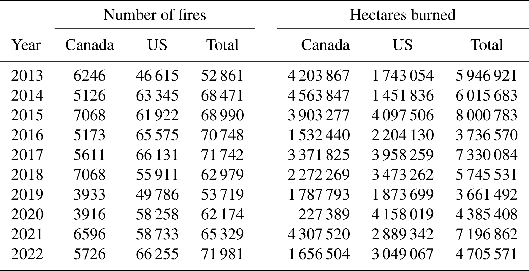
Table A5Comparison of selected NAQFC domain-average monthly statistics for daily mean surface PM2.5 predictions (µg m−3) for 2014 and 2015 (from Lee et al., 2017) with domain-average seasonal statistics for RAQDPS010 forecasts for hourly mean surface PM2.5 predictions (µg m−3) for spring (MAM) and summer (JJA) 2014 and RAQDPS011 forecasts for winter (DJF) 2015 (from Moran et al., 2021a).
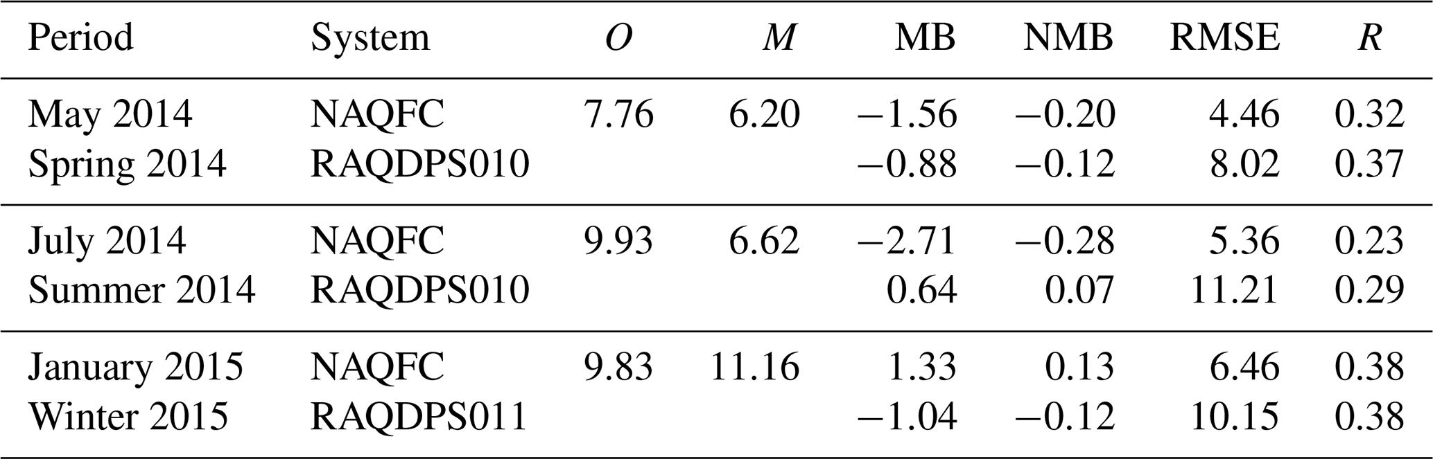
Version 5.1 of the GEM numerical weather prediction model code used by the RAQDPS023 is free software which can be redistributed and/or modified under the terms of version 2.1 of the GNU Lesser General Public License as published by the Free Software Foundation. The GEM source code has been developed by the Meteorological Research Division of ECCC. This code is available for download from https://doi.org/10.5281/zenodo.17782580 (ECCC, 2025b).
MACH, the atmospheric chemistry library for the GEM model (© 2007–2021, Air Quality Research Division and National Prediction Operations Division, Environment and Climate Change Canada), is free software that can be redistributed and/or modified under the terms of the GNU Lesser General Public License as published by the Free Software Foundation – either version 2.1 of the license or any later version. The GEM-MACH version 3.1.0.0 code used by the RAQDPS023 can be downloaded from website https://doi.org/10.5281/zenodo.15330612 (Savic-Jovcic et al., 2025). Related documentation is also available on that website, including information about key input and configuration files and copies of several relevant reports. The GEM-MACH v3.1.1.2 source code for the RAQDPS024, an equivalent version to the RAQDPS023 that went into operation after a migration to a new ECCC high-performance computer system in June 2022, is available at https://doi.org/10.5281/zenodo.13952893 (GEM-MACH development team, 2022).
The CFFEPS version 4.1 code that was used by the RAQDPS-FW023 and RAQDPS-FW024 is free software that can be redistributed and/or modified under the terms of the GNU Lesser General Public License, either version 2.1 or any later version, as published by the Free Software Foundation. It is available to download from website https://doi.org/10.5281/zenodo.15305591 (Anderson and Chen, 2021).
Data sources for the AQ measurement data sets used in this study are listed in Table S2a of the Supplement. Multiple sets of files containing (i) the “raw” measurements that were used in this study, (ii) intermediate measurement files after necessary unit conversions and proxy calculations, (iii) filtered measurement files after application of validity and temporal completeness checks, and (iv) final, evaluation-ready, paired model-measurement files after temporal aggregation for data pooling and filtering for reconstructed mass completeness are available from https://doi.org/10.5281/zenodo.16944371 (Lupu and Moran, 2025). This data repository also contains a complete set of the output files of evaluation scores that were the basis for all of the evaluation-related tables and figures presented in this paper.
A package of seasonal and annual model-predicted gridded surface concentration fields and dry, wet, and total acidic deposition fields for the 2013–2016 simulations is available from the website https://doi.org/10.5281/zenodo.16970403 (Moran and Savic-Jovcic, 2025). Some of the archived model hourly output fields used to create this package were also used by Cathcart et al. (2025) and Robichaud et al. (2025, 2026) in their recent papers.
All other data sets used in this work are available upon request from the authors. Please contact one of the corresponding authors to make a request.
Lastly, a supplement related to this article is available on-line at https://doi.org/10.5281/zenodo.19489036 (Moran and Lupu, 2026).
MDM was the science lead for the development of the online RAQDPS from the RAQDPS001 up to the RAQDPS023 and was the co-supervisor for all operational deliveries from 2009 to 2021. He conceived the objectives and scope of this study, oversaw the evaluations of the RAQDPS023, and prepared the initial and final versions of this paper. AL assisted with the 2013–2016 simulations, obtained all AQ measurement data sets, developed all measurement data processing and evaluation scripts, and generated all evaluation tables and data-related figures for the 2013–2016 and 2021/2022 annual simulations, VSJ developed and maintained RAQDPS code and scripts, performed the 2013–2016 annual simulations, and prepared model-related figures and analyses. JZ performed the 2010–2019 operational evaluation, and JZ, QZ, EIB, and RM generated the 2013–2016 and 2021/2022 anthropogenic emissions files and performed the analyses to construct Tables 1 and S1 and Fig. S1. CAS led the migration from the RAQDPS023 to the RAQDPS024 on the new CMC supercomputers in June 2022 and the development of the RAQDPS025, which became operational in June 2024. SM has been the co-supervisor for all operational deliveries of the RAQDPS with the assistance of VSJ, JC, KM, RMA, and DK. JC led the development and delivery of the RAQDPS-FW023 and all CFFEPS versions with the assistance of KM and RMA. PMM oversaw operational evaluation of North American NRT AQ forecasts at ECCC for GAFIS. Lastly, AL, VSJ, JZ, RM, CAS, JC, QZ, EIB, SM, and RMA reviewed the manuscript.
The authors would like to thank Ayodeji Akingunola, David Anselmo, Didier Davignon, Annie Duhamel, Samuel Gilbert, Hugo Landry, Jessica Miville, David Niemi, Radenko Pavlovic, Si-Jun Peng, Jacinthe Racine, and Mourad Sassi of ECCC for their contributions to this project. We appreciate the generosity of Kristen Foley, Alison Eyth, and their colleagues at the US EPA and General Dynamics Information Technology for providing early access to the EQUATES emissions data set (Foley et al., 2023). Access to a host of AQ measurement data sets was key to this study (see Table S2a), and we thank (i) ECCC for the use of daily filter pack and precipitation–chemistry observations from the CAPMoN network, (ii) ECCC and the provincial, territorial, and regional government NAPS partners for the use of their NAPS network ambient AQ observations, (iii) the US NADP network for the use of observations from the AMoN and NTN networks, (iv) the US EPA for use of observations from the CASTNET and CSN networks and the AQS, (v) the US EPA, the US National Park Service, and other federal, state, and tribal partners for use of observations from the IMPROVE network, and (vi) the US EPA and its state and local, tribal, federal, and Canadian and Mexican partners (https://www.airnow.gov/partners/, last access: 6 April 2026) for the use of near-real-time observations from the AirNow metanetwork. Alexandru Lupu thanks Kulbir Banwait, Amanda Cole, Amy Hou, and Bill Sukloff of the ECCC CAPMoN and NAtChem groups for insightful discussions about various AQ measurement datasets. We also appreciate the provision of operational AQ forecasts by NOAA, NASA, ECMWF, and the Finnish Meteorological Institute to ECCC in NRT under the WMO GAFIS initiative. Michael D. Moran would also like to thank Rosa Wu for her continuing support of this paper over multiple years. We note too that we have chosen to use colour-vision-deficiency-friendly, perceptually-uniform colour maps designed by Crameri et al. (2020) for some figures in this paper. Lastly, the authors would like to thank two anonymous reviewers for their constructive comments that helped to improve the manuscript and the topic editor, Emmanouil Flaounas, for overseeing the review of two lengthy manuscripts.
The contact author has declared that none of the authors has any competing interests.
Publisher's note: Copernicus Publications remains neutral with regard to jurisdictional claims made in the text, published maps, institutional affiliations, or any other geographical representation in this paper. The authors bear the ultimate responsibility for providing appropriate place names. Views expressed in the text are those of the authors and do not necessarily reflect the views of the publisher.
This paper was edited by Emmanouil Flaounas and reviewed by two anonymous referees.
Ames, R. B. and Malm, W. C.: Comparison of sulfate and nitrate particle mass concentrations measured by IMPROVE and the CDN, Atmos. Environ., 35, 905–916, https://doi.org/10.1016/S1352-2310(00)00369-1, 2001.
Anderson, K. and Chen, J.: Canadian Fire Emissions Prediction System (CFFEPS) v4.1, Environment and Climate Change Canada, Zenodo [code], https://doi.org/10.5281/zenodo.15305591, 2021.
Ansari, A. S. and Pandis, S. N.: Response of inorganic PM to precursor concentrations, Environ. Sci. Technol., 32, 2706–2714, https://doi.org/10.1021/es971130j, 1998.
Appel, K. W., Bhave, P. V., Gilliland, A. B., Sarwar, G., and Roselle, S. J.: Evaluation of the Community Multiscale Air Quality (CMAQ) model version 4.5: Sensitivities impacting model performance; Part II – particulate matter, Atmos. Environ., 42, 6057–6066, https://doi.org/10.1016/j.atmosenv.2008.03.036, 2008.
Appel, K. W., Foley, K. M., Bash, J. O., Pinder, R. W., Dennis, R. L., Allen, D. J., and Pickering, K.: A multi-resolution assessment of the Community Multiscale Air Quality (CMAQ) model v4.7 wet deposition estimates for 2002–2006, Geosci. Model Dev., 4, 357–371, https://doi.org/10.5194/gmd-4-357-2011, 2011.
Appel, K. W., Pouliot, G. A., Simon, H., Sarwar, G., Pye, H. O. T., Napelenok, S. L., Akhtar, F., and Roselle, S. J.: Evaluation of dust and trace metal estimates from the Community Multiscale Air Quality (CMAQ) model version 5.0, Geosci. Model Dev., 6, 883–899, https://doi.org/10.5194/gmd-6-883-2013, 2013.
Appel, K. W., Napelenok, S. L., Foley, K. M., Pye, H. O. T., Hogrefe, C., Luecken, D. J., Bash, J. O., Roselle, S. J., Pleim, J. E., Foroutan, H., Hutzell, W. T., Pouliot, G. A., Sarwar, G., Fahey, K. M., Gantt, B., Gilliam, R. C., Heath, N. K., Kang, D., Mathur, R., Schwede, D. B., Spero, T. L., Wong, D. C., and Young, J. O.: Description and evaluation of the Community Multiscale Air Quality (CMAQ) modeling system version 5.1, Geosci. Model Dev., 10, 1703–1732, https://doi.org/10.5194/gmd-10-1703-2017, 2017.
Appel, K. W., Bash, J. O., Fahey, K. M., Foley, K. M., Gilliam, R. C., Hogrefe, C., Hutzell, W. T., Kang, D., Mathur, R., Murphy, B. N., Napelenok, S. L., Nolte, C. G., Pleim, J. E., Pouliot, G. A., Pye, H. O. T., Ran, L., Roselle, S. J., Sarwar, G., Schwede, D. B., Sidi, F. I., Spero, T. L., and Wong, D. C.: The Community Multiscale Air Quality (CMAQ) model versions 5.3 and 5.3.1: system updates and evaluation, Geosci. Model Dev., 14, 2867–2897, https://doi.org/10.5194/gmd-14-2867-2021, 2021.
Astitha, M., Kioutsioukis, I., Fisseha, G. A., Bianconi, R., Bieser, J., Christensen, J. H., Cooper, O. R., Galmarini, S., Hogrefe, C., Im, U., Johnson, B., Liu, P., Nopmongcol, U., Petropavlovskikh, I., Solazzo, E., Tarasick, D. W., and Yarwood, G.: Seasonal ozone vertical profiles over North America using the AQMEII3 group of air quality models: model inter-comparison and stratospheric intrusions, Atmos. Chem. Phys., 18, 13925–13945, https://doi.org/10.5194/acp-18-13925-2018, 2018.
Bachmann, J. D.: Tackling multi-pollutant particles, EM Air Waste Manag. Assoc. Mag. Environ. Manag., 6–9, https://www.researchgate.net/publication/268280224_Tackling_Multi-pollutant_Particles (last access: 6 April 2026), 2013.
Bencala, K. E. and Seinfeld, J. H.: An air quality model performance assessment package, Atmos. Environ., 13, 1181–1185, https://doi.org/10.1016/0004-6981(79)90043-X, 1979.
Benish, S. E., Bash, J. O., Foley, K. M., Appel, K. W., Hogrefe, C., Gilliam, R., and Pouliot, G.: Long-term regional trends of nitrogen and sulfur deposition in the United States from 2002 to 2017, Atmos. Chem. Phys., 22, 12749–12767, https://doi.org/10.5194/acp-22-12749-2022, 2022.
Bermejo, R. and Conde, J.: A conservative quasi-monotone semi-Lagrangian scheme, Mon. Weather Rev., 130, 423–430, https://doi.org/10.1175/1520-0493(2002)130<0423:ACQMSL>2.0.CO;2, 2002.
Biswas, J., Hogrefe, C., Rao, S. T., Hao, W., and Sistla, G.: Evaluating the performance of regional-scale photochemical modeling systems. Part III – Precursor predictions, Atmos. Environ., 35, 6129–6149, https://doi.org/10.1016/S1352-2310(01)00401-0, 2001.
Bloom, S. C., Takacs, L. L., da Silva, A. M., and Ledvina, D.: Data assimilation using incremental analysis updates, Mon. Weather Rev., 124, 1256–1271, https://doi.org/10.1175/1520-0493(1996)124<1256:DAUIAU>2.0.CO;2, 1996.
Borrego, C., Monteiro, A., Ferreira, J., Miranda, A. I., Costa, A. M., Carvalho, A. C., and Lopes, M.: Procedures for estimation of modelling uncertainty in air quality assessment, Environ. Int., 34, 613–620, https://doi.org/10.1016/j.envint.2007.12.005, 2008.
Brasseur, G. P. and Kumar, R.: Chemical weather and chemical climate, AGU Adv., 2, e2021AV000399, https://doi.org/10.1029/2021AV000399, 2021.
Cai, C., Hogrefe, C., Katsafados, P., Kallos, G., Beauharnois, M., Schwab, J. J., Ren, X., Brune, W. H., Zhou, X., He, Y., and Demerjian, K. L.: Performance evaluation of an air quality forecast modeling system for a summer and winter season – Photochemical oxidants and their precursors, Atmos. Environ., 42, 8585–8599, https://doi.org/10.1016/j.atmosenv.2008.08.029, 2008.
Campbell, P. C., Tang, Y., Lee, P., Baker, B., Tong, D., Saylor, R., Stein, A., Huang, J., Huang, H.-C., Strobach, E., McQueen, J., Pan, L., Stajner, I., Sims, J., Tirado-Delgado, J., Jung, Y., Yang, F., Spero, T. L., and Gilliam, R. C.: Development and evaluation of an advanced National Air Quality Forecasting Capability using the NOAA Global Forecast System version 16, Geosci. Model Dev., 15, 3281–3313, https://doi.org/10.5194/gmd-15-3281-2022, 2022.
Canadian Interagency Forest Fire Centre: Canada Report 2022, 15 pp., https://ciffc.ca/publications/canada-reports/ (last access: 6 April 2026), 2023.
Caron, J.-F., Milewski, T., Buehner, M., Fillion, L., Reszka, M., Macpherson, S., and St-James, J.: Implementation of deterministic weather forecasting systems based on ensemble–variational data assimilation at Environment Canada. Part II: The regional system, Mon. Weather Rev., 143, 2560–2580, https://doi.org/10.1175/MWR-D-14-00353.1, 2015.
Cathcart, H., Aherne, J., Moran, M. D., Savic-Jovcic, V., Makar, P. A., and Cole, A.: Estimates of critical loads and exceedances of acidity and nutrient nitrogen for mineral soils in Canada for 2014–2016 average annual sulfur and nitrogen atmospheric deposition, Biogeosciences, 22, 535–554, https://doi.org/10.5194/bg-22-535-2025, 2025.
Chai, T., Kim, H.-C., Lee, P., Tong, D., Pan, L., Tang, Y., Huang, J., McQueen, J., Tsidulko, M., and Stajner, I.: Evaluation of the United States National Air Quality Forecast Capability experimental real-time predictions in 2010 using Air Quality System ozone and NO2 measurements, Geosci. Model Dev., 6, 1831–1850, https://doi.org/10.5194/gmd-6-1831-2013, 2013.
Chan, E. A. W., Gantt, B., and McDow, S.: The reduction of summer sulfate and switch from summertime to wintertime PM2.5 concentration maxima in the United States, Atmos. Environ., 175, 25–32, https://doi.org/10.1016/j.atmosenv.2017.11.055, 2018.
Chang, J. C. and Hanna, S. R.: Air quality model performance evaluation, Meteorol. Atmos. Phys., 87, https://doi.org/10.1007/s00703-003-0070-7, 2004.
Chen, J. and Menelaou, K.: Regional Air Quality Deterministic Prediction System with near-real-time wildfire emissions (RAQDPSFW): Upgrade to version 023, Technical note, November, Canadian Centre for Meteorological and Environmental Prediction, Montreal, 31 pp., https://collaboration.cmc.ec.gc.ca/cmc/CMOI/product_guide/docs/tech_notes/technote_raqdpsfw_e.pdf (last access: 6 April 2026), 2021.
Chen, J., Anderson, K., Pavlovic, R., Moran, M. D., Englefield, P., Thompson, D. K., Munoz-Alpizar, R., and Landry, H.: The FireWork v2.0 air quality forecast system with biomass burning emissions from the Canadian Forest Fire Emissions Prediction System v2.03, Geosci. Model Dev., 12, 3283–3310, https://doi.org/10.5194/gmd-12-3283-2019, 2019.
Chen, X., Zhang, Y., Wang, K., Tong, D., Lee, P., Tang, Y., Huang, J., Campbell, P. C., Mcqueen, J., Pye, H. O. T., Murphy, B. N., and Kang, D.: Evaluation of the offline-coupled GFSv15–FV3–CMAQv5.0.2 in support of the next-generation National Air Quality Forecast Capability over the contiguous United States, Geosci. Model Dev., 14, 3969–3993, https://doi.org/10.5194/gmd-14-3969-2021, 2021.
Chow, J. C.: Measurement methods to determine compliance with ambient air quality standards for suspended particles, J. Air Waste Manage. Assoc., 45, 320–382, https://doi.org/10.1080/10473289.1995.10467369, 1995.
Chow, J. C., Lowenthal, D. H., Chen, L.-W. A., Wang, X., and Watson, J. G.: Mass reconstruction methods for PM2.5: a review, Air Qual. Atmos. Health, 8, 243–263, https://doi.org/10.1007/s11869-015-0338-3, 2015.
Chuang, M.-T., Zhang, Y., and Kang, D.: Application of WRF/Chem-MADRID for real-time air quality forecasting over the southeastern United States, Atmos. Environ., 45, 6241–6250, https://doi.org/10.1016/j.atmosenv.2011.06.071, 2011.
Clifton, O. E., Schwede, D., Hogrefe, C., Bash, J. O., Bland, S., Cheung, P., Coyle, M., Emberson, L., Flemming, J., Fredj, E., Galmarini, S., Ganzeveld, L., Gazetas, O., Goded, I., Holmes, C. D., Horváth, L., Huijnen, V., Li, Q., Makar, P. A., Mammarella, I., Manca, G., Munger, J. W., Pérez-Camanyo, J. L., Pleim, J., Ran, L., San Jose, R., Silva, S. J., Staebler, R., Sun, S., Tai, A. P. K., Tas, E., Vesala, T., Weidinger, T., Wu, Z., and Zhang, L.: A single-point modeling approach for the intercomparison and evaluation of ozone dry deposition across chemical transport models (Activity 2 of AQMEII4), Atmos. Chem. Phys., 23, 9911–9961, https://doi.org/10.5194/acp-23-9911-2023, 2023.
CMC-RAQDPS-023: The Regional Air Quality Deterministic Prediction System (RAQDPS) version 023 and the Regional Air Quality Deterministic Prediction System with Near-Real-Time Wildfire Emissions (RAQDPSFW) version 023 of the Meteorological Service of Canada (MSC): Technical Specifications Document, November, Canadian Centre for Meteorological and Environmental Prediction, Montreal, 19 pp., https://collaboration.cmc.ec.gc.ca/cmc/cmoi/product_guide/docs/tech_specifications/tech_specifications_RAQDPS_023_e.pdf (last access: 6 April 2026), 2021.
CMC-RAQDPS-025: The Regional Air Quality Deterministic Prediction System (RAQDPS): Upgrade from version 024 to version 025, June, Canadian Centre for Meteorological and Environmental Prediction, Montreal, 89 pp., https://collaboration.cmc.ec.gc.ca/cmc/cmoi/product_guide/docs/tech_notes/technote_raqdps-v25_e.pdf (last access: 6 April 2026), 2024.
CMC-RDPS-8.0.0: The Regional Deterministic Prediction System (RDPS) version 8.0.0 of the Meteorological Service of Canada (MSC): Technical specifications document, December, Canadian Centre for Meteorological and Environmental Prediction, Montreal, 10 pp., https://collaboration.cmc.ec.gc.ca/cmc/cmoi/product_guide/docs/tech_specifications/tech_specifications_RDPS_8.0.0_e.pdf (last access: 6 April 2026), 2021.
Colette, A., Andersson, C., Manders, A., Mar, K., Mircea, M., Pay, M.-T., Raffort, V., Tsyro, S., Cuvelier, C., Adani, M., Bessagnet, B., Bergström, R., Briganti, G., Butler, T., Cappelletti, A., Couvidat, F., D'Isidoro, M., Doumbia, T., Fagerli, H., Granier, C., Heyes, C., Klimont, Z., Ojha, N., Otero, N., Schaap, M., Sindelarova, K., Stegehuis, A. I., Roustan, Y., Vautard, R., Van Meijgaard, E., Vivanco, M. G., and Wind, P.: EURODELTA-Trends, a multi-model experiment of air quality hindcast in Europe over 1990–2010, Geosci. Model Dev., 10, 3255–3276, https://doi.org/10.5194/gmd-10-3255-2017, 2017.
Colette, A., Collin, G., Besson, F., Blot, E., Guidard, V., Meleux, F., Royer, A., Petiot, V., Miller, C., Fermond, O., Jeant, A., Adani, M., Arteta, J., Benedictow, A., Bergström, R., Bowdalo, D., Brandt, J., Briganti, G., Carvalho, A. C., Christensen, J. H., Couvidat, F., D'Elia, I., D'Isidoro, M., Denier Van Der Gon, H., Descombes, G., Di Tomaso, E., Douros, J., Escribano, J., Eskes, H., Fagerli, H., Fatahi, Y., Flemming, J., Friese, E., Frohn, L., Gauss, M., Geels, C., Guarnieri, G., Guevara, M., Guion, A., Guth, J., Hänninen, R., Hansen, K., Im, U., Janssen, R., Jeoffrion, M., Joly, M., Jones, L., Jorba, O., Kadantsev, E., Kahnert, M., Kaminski, J. W., Kouznetsov, R., Kranenburg, R., Kuenen, J., Lange, A. C., Langner, J., Lannuque, V., Macchia, F., Manders, A., Mircea, M., Nyiri, A., Olid, M., Pérez García-Pando, C., Palamarchuk, Y., Piersanti, A., Raux, B., Razinger, M., Robertson, L., Segers, A., Schaap, M., Siljamo, P., Simpson, D., Sofiev, M., Stangel, A., Struzewska, J., Tena, C., Timmermans, R., Tsikerdekis, T., Tsyro, S., Tyuryakov, S., Ung, A., Uppstu, A., Valdebenito, A., Van Velthoven, P., Vitali, L., Ye, Z., Peuch, V.-H., and Rouïl, L.: Copernicus Atmosphere Monitoring Service – Regional Air Quality Production System v1.0, Geosci. Model Dev., 18, 6835–6883, https://doi.org/10.5194/gmd-18-6835-2025, 2025.
Crameri, F., Shephard, G. E., and Heron, P. J.: The misuse of colour in science communication, Nat. Commun., 11, 5444, https://doi.org/10.1038/s41467-020-19160-7, 2020.
Dabek-Zlotorzynska, E., Dann, T. F., Kalyani Martinelango, P., Celo, V., Brook, J. R., Mathieu, D., Ding, L., and Austin, C. C.: Canadian National Air Pollution Surveillance (NAPS) PM2.5 speciation program: Methodology and PM2.5 chemical composition for the years 2003–2008, Atmos. Environ., 45, 673–686, https://doi.org/10.1016/j.atmosenv.2010.10.024, 2011.
Demerjian, K.: A review of national monitoring networks in North America, Atmos. Environ., 34, 1861–1884, https://doi.org/10.1016/S1352-2310(99)00452-5, 2000.
Dennis, R., Fox, T., Fuentes, M., Gilliland, A., Hanna, S., Hogrefe, C., Irwin, J., Rao, S. T., Scheffe, R., Schere, K., Steyn, D., and Venkatram, A.: A framework for evaluating regional-scale numerical photochemical modeling systems, Environ. Fluid Mech., 10, 471–489, https://doi.org/10.1007/s10652-009-9163-2, 2010.
Dennis, R. L. and Downton, M. W.: Evaluation of urban photochemical models for regulatory use, Atmos. Environ. 1967, 18, 2055–2069, https://doi.org/10.1016/0004-6981(84)90192-6, 1984.
Dennis, R. L., McHenry, J. N., Barchet, W. R., Binkowski, F. S., and Byun, D. W.: Correcting RADM's sulfate underprediction: Discovery and correction of model errors and testing the corrections through comparisons against field data, Atmos. Environ. Part Gen. Top., 27, 975–997, https://doi.org/10.1016/0960-1686(93)90012-N, 1993.
Derwent, R., Fraser, A., Abbot, J., Jenkin, M., Willis, P., and Murrells, T.: Evaluating the Performance of Air Quality Models, Department for Environment Food and Rural Affairs, United Kingdom, https://uk-air.defra.gov.uk/assets/documents/reports/cat05/1006241607_100608_MIP_Final_Version.pdf (last access: 6 April 2026), 2010.
Dickerson, R. R., Anderson, D. C., and Ren, X.: On the use of data from commercial NOx analyzers for air pollution studies, Atmos. Environ., 214, 116873, https://doi.org/10.1016/j.atmosenv.2019.116873, 2019.
Dickson, R. J. and Oliver, W. R.: Emissions models for regional air quality studies, Environ. Sci. Technol., 25, 1533–1535, https://doi.org/10.1021/es00021a003, 1991.
Dunlea, E. J., Herndon, S. C., Nelson, D. D., Volkamer, R. M., San Martini, F., Sheehy, P. M., Zahniser, M. S., Shorter, J. H., Wormhoudt, J. C., Lamb, B. K., Allwine, E. J., Gaffney, J. S., Marley, N. A., Grutter, M., Marquez, C., Blanco, S., Cardenas, B., Retama, A., Ramos Villegas, C. R., Kolb, C. E., Molina, L. T., and Molina, M. J.: Evaluation of nitrogen dioxide chemiluminescence monitors in a polluted urban environment, Atmos. Chem. Phys., 7, 2691–2704, https://doi.org/10.5194/acp-7-2691-2007, 2007.
Dye, T. S., Chan, A. C., Anderson, C. B., Strohm, D. E. B., Wayland, R. A., and White, J. E.: From raw air quality data to the nightly news: an overview of how EPA's AirNow program operates, Sixth Conference on Atmospheric Chemistry, 12–14 January 2004, Seattle, Washington, American Meteorological Society, https://ams.confex.com/ams/pdfpapers/72477.pdf (last access: 6 April 2026), 2004.
ECCC: 1990–2016 Air Pollutant Emission Inventory Report, Environment and Climate Change Canada, Gatineau, Quebec, 92 pp., https://publications.gc.ca/collections/collection_2018/eccc/En81-26-2016-eng.pdf (last access: 6 April 2026), 2018.
ECCC: Canada's Air Pollutant Emissions Inventory Report 1990–2023, Environment and Climate Change Canada, Gatineau, Quebec, 72 pp., https://publications.gc.ca/collections/collection_2025/eccc/En81-30-2023-eng.pdf (last access: 6 April 2026), 2025a.
ECCC: Version 5.1 package for the Global Environmental Multiscale (GEM) model (ECCC-ASTD-MRD/gem: 5.1.0), Environment and Climate Change Canada, Zenodo [code], https://doi.org/10.5281/zenodo.17782580, 2025b.
Eder, B., Kang, D., Mathur, R., Yu, S., and Schere, K.: An operational evaluation of the Eta–CMAQ air quality forecast model, Atmos. Environ., 40, 4894–4905, https://doi.org/10.1016/j.atmosenv.2005.12.062, 2006.
Eder, B., Kang, D., Mathur, R., Pleim, J., Yu, S., Otte, T., and Pouliot, G.: A performance evaluation of the National Air Quality Forecast Capability for the summer of 2007, Atmos. Environ., 43, 2312–2320, https://doi.org/10.1016/j.atmosenv.2009.01.033, 2009.
Eder, B., Kang, D., Rao, S. T., Mathur, R., Yu, S., Otte, T., Schere, K., Wayland, R., Jackson, S., Davidson, P., McQueen, J., and Bridgers, G.: Using National Air Quality Forecast Guidance to develop local Air Quality Index forecasts, B. Am. Meteorol. Soc., 91, 313–326, https://doi.org/10.1175/2009BAMS2734.1, 2010.
Emery, C., Liu, Z., Russell, A. G., Odman, M. T., Yarwood, G., and Kumar, N.: Recommendations on statistics and benchmarks to assess photochemical model performance, J. Air Waste Manage. Assoc., 67, 582–598, https://doi.org/10.1080/10962247.2016.1265027, 2017.
Entekhabi, D., Reichle, R. H., Koster, R. D., and Crow, W. T.: Performance metrics for soil moisture retrievals and application requirements, J. Hydrometeorol., 11, 832–840, https://doi.org/10.1175/2010JHM1223.1, 2010.
Feng, J., Chan, E., and Vet, R.: Air quality in the eastern United States and eastern Canada for 1990–2015: 25 years of change in response to emission reductions of SO2 and NOx in the region, Atmos. Chem. Phys., 20, 3107–3134, https://doi.org/10.5194/acp-20-3107-2020, 2020.
Feng, J., Cole, A., Wetherbee, G. A., and Banwait, K.: Inter-comparison of measurements of inorganic chemical components in precipitation from NADP and CAPMoN at collocated sites in the USA and Canada during 1986–2019, Environ. Monit. Assess., 195, 1333, https://doi.org/10.1007/s10661-023-11771-z, 2023.
Fillion, L., Mitchell, H. L., Ritchie, H., and Staniforth, A.: The impact of a digital filter finalization technique in a global data assimilation system, Tellus A, 47, 304–323, https://doi.org/10.1034/j.1600-0870.1995.t01-2-00002.x, 1995.
Fillion, L., Tanguay, M., Lapalme, E., Denis, B., Desgagné, M., Lee, V., Ek, N., Liu, Z., Lajoie, M., Caron, J.-F., and Pagé, C.: The Canadian Regional Data Assimilation and Forecasting System, Weather Forecast., 25, 1645–1669, https://doi.org/10.1175/2010WAF2222401.1, 2010.
Foley, K. M., Hogrefe, C., Pouliot, G., Possiel, N., Roselle, S. J., Simon, H., and Timin, B.: Dynamic evaluation of CMAQ part I: Separating the effects of changing emissions and changing meteorology on ozone levels between 2002 and 2005 in the eastern US, Atmos. Environ., 103, 247–255, https://doi.org/10.1016/j.atmosenv.2014.12.038, 2015.
Foley, K. M., Pouliot, G. A., Eyth, A., Aldridge, M. F., Allen, C., Appel, K. W., Bash, J. O., Beardsley, M., Beidler, J., Choi, D., Farkas, C., Gilliam, R. C., Godfrey, J., Henderson, B. H., Hogrefe, C., Koplitz, S. N., Mason, R., Mathur, R., Misenis, C., Possiel, N., Pye, H. O. T., Reynolds, L., Roark, M., Roberts, S., Schwede, D. B., Seltzer, K. M., Sonntag, D., Talgo, K., Toro, C., Vukovich, J., Xing, J., and Adams, E.: 2002–2017 anthropogenic emissions data for air quality modeling over the United States, Data Brief, 47, 109022, https://doi.org/10.1016/j.dib.2023.109022, 2023.
Foroutan, H., Young, J., Napelenok, S., Ran, L., Appel, K. W., Gilliam, R. C., and Pleim, J. E.: Development and evaluation of a physics-based windblown dust emission scheme implemented in the CMAQ modeling system, J. Adv. Model. Earth Syst., 9, 585–608, https://doi.org/10.1002/2016MS000823, 2017.
Frank, N. H.: Retained nitrate, hydrated sulfates, and carbonaceous mass in Federal Reference Method fine particulate matter for six eastern U.S. cities, J. Air Waste Manage. Assoc., 56, 500–511, https://doi.org/10.1080/10473289.2006.10464517, 2006.
Fruin, S., Urman, R., Lurmann, F., McConnell, R., Gauderman, J., Rappaport, E., Franklin, M., Gilliland, F. D., Shafer, M., Gorski, P., and Avol, E.: Spatial variation in particulate matter components over a large urban area, Atmos. Environ., 83, 211–219, https://doi.org/10.1016/j.atmosenv.2013.10.063, 2014.
Galmarini, S., Bonnardot, F., Jones, A., Potempski, S., Robertson, L., and Martet, M.: Multi-model vs. EPS-based ensemble atmospheric dispersion simulations: A quantitative assessment on the ETEX-1 tracer experiment case, Atmos. Environ., 44, 3558–3567, https://doi.org/10.1016/j.atmosenv.2010.06.003, 2010.
Galmarini, S., Makar, P., Clifton, O. E., Hogrefe, C., Bash, J. O., Bellasio, R., Bianconi, R., Bieser, J., Butler, T., Ducker, J., Flemming, J., Hodzic, A., Holmes, C. D., Kioutsioukis, I., Kranenburg, R., Lupascu, A., Perez-Camanyo, J. L., Pleim, J., Ryu, Y.-H., San Jose, R., Schwede, D., Silva, S., and Wolke, R.: Technical note: AQMEII4 Activity 1: evaluation of wet and dry deposition schemes as an integral part of regional-scale air quality models, Atmos. Chem. Phys., 21, 15663–15697, https://doi.org/10.5194/acp-21-15663-2021, 2021.
Gan, C. M., Binkowski, F., Pleim, J., Xing, J., Wong, D., Mathur, R., and Gilliam, R.: Assessment of the aerosol optics component of the coupled WRF–CMAQ model using CARES field campaign data and a single column model, Atmos. Environ., 115, 670–682, https://doi.org/10.1016/j.atmosenv.2014.11.028, 2015.
Gantt, B.: 10 Years (2011–2020) of the NCore Network: FEMs vs FRMs, 2022 National Ambient Air Monitoring Conference, 22–25 August 2022, Pittsburgh, Pennsylvania, https://www.epa.gov/system/files/documents/2022-10/Gantt_Brett_Wed1030.pdf (last access: 6 April 2026), 2022.
Gaudel, A., Cooper, O. R., Ancellet, G., Barret, B., Boynard, A., Burrows, J. P., Clerbaux, C., Coheur, P.-F., Cuesta, J., Cuevas, E., Doniki, S., Dufour, G., Ebojie, F., Foret, G., Garcia, O., Granados-Muñoz, M. J., Hannigan, J. W., Hase, F., Hassler, B., Huang, G., Hurtmans, D., Jaffe, D., Jones, N., Kalabokas, P., Kerridge, B., Kulawik, S., Latter, B., Leblanc, T., Le Flochmoën, E., Lin, W., Liu, J., Liu, X., Mahieu, E., McClure-Begley, A., Neu, J. L., Osman, M., Palm, M., Petetin, H., Petropavlovskikh, I., Querel, R., Rahpoe, N., Rozanov, A., Schultz, M. G., Schwab, J., Siddans, R., Smale, D., Steinbacher, M., Tanimoto, H., Tarasick, D. W., Thouret, V., Thompson, A. M., Trickl, T., Weatherhead, E., Wespes, C., Worden, H. M., Vigouroux, C., Xu, X., Zeng, G., and Ziemke, J.: Tropospheric Ozone Assessment Report: Present-day distribution and trends of tropospheric ozone relevant to climate and global atmospheric chemistry model evaluation, Elem. Sci. Anthr., 6, 39, https://doi.org/10.1525/elementa.291, 2018.
GEM-MACH development team: GEM-MACHv3.1.1.2, Zenodo [code], https://doi.org/10.5281/zenodo.13952893, 2022.
Gilliam, R. C., Hogrefe, C., Godowitch, J. M., Napelenok, S., Mathur, R., and Rao, S. T.: Impact of inherent meteorology uncertainty on air quality model predictions, J. Geophys. Res.-Atmos., 120, https://doi.org/10.1002/2015JD023674, 2015.
Gilliam, R. C., Herwehe, J. A., Bullock, O. R., Pleim, J. E., Ran, L., Campbell, P. C., and Foroutan, H.: Establishing the suitability of the Model for Prediction Across Scales for global retrospective air quality modeling, J. Geophys. Res.-Atmos., 126, e2020JD033588, https://doi.org/10.1029/2020JD033588, 2021.
Gilliland, A. B., Hogrefe, C., Pinder, R. W., Godowitch, J. M., Foley, K. L., and Rao, S. T.: Dynamic evaluation of regional air quality models: Assessing changes in O3 stemming from changes in emissions and meteorology, Atmos. Environ., 42, 5110–5123, https://doi.org/10.1016/j.atmosenv.2008.02.018, 2008.
Godowitch, J. M., Pouliot, G. A., and Trivikrama Rao, S.: Assessing multi-year changes in modeled and observed urban NOx concentrations from a dynamic model evaluation perspective, Atmos. Environ., 44, 2894–2901, https://doi.org/10.1016/j.atmosenv.2010.04.040, 2010.
Godowitch, J. M., Gilliam, R. C., and Rao, S. T.: Diagnostic evaluation of ozone production and horizontal transport in a regional photochemical air quality modeling system, Atmos. Environ., 45, 3977–3987, https://doi.org/10.1016/j.atmosenv.2011.04.062, 2011.
Hand, J. L., Schichtel, B. A., Pitchford, M., Malm, W. C., and Frank, N. H.: Seasonal composition of remote and urban fine particulate matter in the United States, J. Geophys. Res.-Atmos., 117, https://doi.org/10.1029/2011JD017122, 2012.
Hand, J. L., Schichtel, B. A., Malm, W. C., and Frank, N. H.: Spatial and temporal trends in PM 2.5 organic and elemental carbon across the United States, Adv. Meteorol., 2013, 1–13, https://doi.org/10.1155/2013/367674, 2013.
Hand, J. L., Prenni, A. J., Schichtel, B. A., Malm, W. C., and Chow, J. C.: Trends in remote PM2.5 residual mass across the United States: Implications for aerosol mass reconstruction in the IMPROVE network, Atmos. Environ., 203, 141–152, https://doi.org/10.1016/j.atmosenv.2019.01.049, 2019.
Hand, J. L., Prenni, A. J., and Schichtel, B. A.: Trends in seasonal mean speciated aerosol composition in remote areas of the United States from 2000 through 2021, J. Geophys. Res.-Atmos., 129, e2023JD039902, https://doi.org/10.1029/2023JD039902, 2024.
Hanna, S. R., Russell, A. G., Wilkinson, J. G., Vukovich, J., and Hansen, D. A.: Monte Carlo estimation of uncertainties in BEIS3 emission outputs and their effects on uncertainties in chemical transport model predictions, J. Geophys. Res., 110, D01302, https://doi.org/10.1029/2004JD004986, 2005.
He, H., Vinnikov, K. Y., Krotkov, N. A., Edgerton, E. S., Schwab, J. J., and Dickerson, R. R.: Chemical climatology of atmospheric pollutants in the eastern United States: Seasonal/diurnal cycles and contrast under clear/cloudy conditions for remote sensing, Atmos. Environ., 206, 85–107, https://doi.org/10.1016/j.atmosenv.2019.03.003, 2019.
Hogrefe, C., Rao, S. T., Kasibhatla, P., Hao, W., Sistla, G., Mathur, R., and McHenry, J.: Evaluating the performance of regional-scale photochemical modeling systems: Part II – ozone predictions, Atmos. Environ., 35, 4175–4188, https://doi.org/10.1016/S1352-2310(01)00183-2, 2001a.
Hogrefe, C., Rao, S. T., Kasibhatla, P., Kallos, G., Tremback, C. J., Hao, W., Olerud, D., Xiu, A., McHenry, J., and Alapaty, K.: Evaluating the performance of regional-scale photochemical modeling systems: Part I – meteorological predictions, Atmos. Environ., 35, 4159–4174, https://doi.org/10.1016/S1352-2310(01)00182-0, 2001b.
Hogrefe, C., Pouliot, G., Wong, D., Torian, A., Roselle, S., Pleim, J., and Mathur, R.: Annual application and evaluation of the online coupled WRF–CMAQ system over North America under AQMEII phase 2, Atmos. Environ., 115, 683–694, https://doi.org/10.1016/j.atmosenv.2014.12.034, 2015.
Hogrefe, C., Galmarini, S., Makar, P. A., Kioutsioukis, I., Clifton, O. E., Alyuz, U., Bash, J. O., Bellasio, R., Bianconi, R., Butler, T., Cheung, P., Hodzic, A., Kranenburg, R., Lupascu, A., Momoh, K., Perez-Camanyo, J. L., Pleim, J. E., Ryu, Y.-H., San Jose, R., Schaap, M., Schwede, D. B., and Sokhi, R.: A diagnostic intercomparison of modeled ozone dry deposition over North America and Europe using AQMEII4 regional-scale simulations, Atmos. Chem. Phys., 25, 12629–12656, https://doi.org/10.5194/acp-25-12629-2025, 2025.
Holden, A. S., Sullivan, A. P., Munchak, L. A., Kreidenweis, S. M., Schichtel, B. A., Malm, W. C., and Collett, J. L.: Determining contributions of biomass burning and other sources to fine particle contemporary carbon in the western United States, Atmos. Environ., 45, 1986–1993, https://doi.org/10.1016/j.atmosenv.2011.01.021, 2011.
Houyoux, M. R., Vukovich, J. M., Coats, C. J., Wheeler, N. J. M., and Kasibhatla, P. S.: Emission inventory development and processing for the Seasonal Model for Regional Air Quality (SMRAQ) project, J. Geophys. Res.-Atmos., 105, 9079–9090, https://doi.org/10.1029/1999JD900975, 2000.
Huang, J., McQueen, J., Wilczak, J., Djalalova, I., Stajner, I., Shafran, P., Allured, D., Lee, P., Pan, L., Tong, D., Huang, H.-C., DiMego, G., Upadhayay, S., and Delle Monache, L.: Improving NOAA NAQFC PM2.5 predictions with a bias correction approach, Weather Forecast., 32, 407–421, https://doi.org/10.1175/WAF-D-16-0118.1, 2017.
Huang, L., Zhu, Y., Zhai, H., Xue, S., Zhu, T., Shao, Y., Liu, Z., Emery, C., Yarwood, G., Wang, Y., Fu, J., Zhang, K., and Li, L.: Recommendations on benchmarks for numerical air quality model applications in China – Part 1: PM2.5 and chemical species, Atmos. Chem. Phys., 21, 2725–2743, https://doi.org/10.5194/acp-21-2725-2021, 2021.
Hystad, P., Setton, E., Cervantes, A., Poplawski, K., Deschenes, S., Brauer, M., Van Donkelaar, A., Lamsal, L., Martin, R., Jerrett, M., and Demers, P.: Creating national air pollution models for population exposure assessment in Canada, Environ. Health Perspect., 119, 1123–1129, https://doi.org/10.1289/ehp.1002976, 2011.
Im, U., Bianconi, R., Solazzo, E., Kioutsioukis, I., Badia, A., Balzarini, A., Baró, R., Bellasio, R., Brunner, D., Chemel, C., Curci, G., Flemming, J., Forkel, R., Giordano, L., Jiménez-Guerrero, P., Hirtl, M., Hodzic, A., Honzak, L., Jorba, O., Knote, C., Kuenen, J. J. P., Makar, P. A., Manders-Groot, A., Neal, L., Pérez, J. L., Pirovano, G., Pouliot, G., San Jose, R., Savage, N., Schroder, W., Sokhi, R. S., Syrakov, D., Torian, A., Tuccella, P., Werhahn, J., Wolke, R., Yahya, K., Zabkar, R., Zhang, Y., Zhang, J., Hogrefe, C., and Galmarini, S.: Evaluation of operational on-line-coupled regional air quality models over Europe and North America in the context of AQMEII phase 2. Part I: Ozone, Atmos. Environ., 115, 404–420, https://doi.org/10.1016/j.atmosenv.2014.09.042, 2015a.
Im, U., Bianconi, R., Solazzo, E., Kioutsioukis, I., Badia, A., Balzarini, A., Baró, R., Bellasio, R., Brunner, D., Chemel, C., Curci, G., Denier Van Der Gon, H., Flemming, J., Forkel, R., Giordano, L., Jiménez-Guerrero, P., Hirtl, M., Hodzic, A., Honzak, L., Jorba, O., Knote, C., Makar, P. A., Manders-Groot, A., Neal, L., Pérez, J. L., Pirovano, G., Pouliot, G., San Jose, R., Savage, N., Schroder, W., Sokhi, R. S., Syrakov, D., Torian, A., Tuccella, P., Wang, K., Werhahn, J., Wolke, R., Zabkar, R., Zhang, Y., Zhang, J., Hogrefe, C., and Galmarini, S.: Evaluation of operational online-coupled regional air quality models over Europe and North America in the context of AQMEII phase 2. Part II: Particulate matter, Atmos. Environ., 115, 421–441, https://doi.org/10.1016/j.atmosenv.2014.08.072, 2015b.
Jaeglé, L., Shah, V., Thornton, J. A., Lopez-Hilfiker, F. D., Lee, B. H., McDuffie, E. E., Fibiger, D., Brown, S. S., Veres, P., Sparks, T. L., Ebben, C. J., Wooldridge, P. J., Kenagy, H. S., Cohen, R. C., Weinheimer, A. J., Campos, T. L., Montzka, D. D., Digangi, J. P., Wolfe, G. M., Hanisco, T., Schroder, J. C., Campuzano-Jost, P., Day, D. A., Jimenez, J. L., Sullivan, A. P., Guo, H., and Weber, R. J.: Nitrogen oxides, emissions, chemistry, deposition, and export over the northeast United States during the WINTER aircraft campaign, J. Geophys. Res.-Atmos., 123, https://doi.org/10.1029/2018JD029133, 2018.
Jaffe, D., Bertschi, I., Jaegle, L., Novelli, P., Reid, J. S., Tanimoto, H., Vingarzan, R., and Westphal, D. L.: Long-range transport of Siberian biomass burning emissions and impact on surface ozone in western North America, Geophys. Res. Lett., 31, L16106, https://doi.org/10.1029/2004GL020093, 2004.
Jain, P., Sharma, A. R., Acuna, D. C., Abatzoglou, J. T., and Flannigan, M.: Record-breaking fire weather in North America in 2021 was initiated by the Pacific northwest heat dome, Commun. Earth Environ., 5, 202, https://doi.org/10.1038/s43247-024-01346-2, 2024.
Jerrett, M., Arain, A., Kanaroglou, P., Beckerman, B., Potoglou, D., Sahsuvaroglu, T., Morrison, J., and Giovis, C.: A review and evaluation of intraurban air pollution exposure models, J. Exp. Sci. Environ. Epidemiol., 15, 185–204, https://doi.org/10.1038/sj.jea.7500388, 2005.
Kajino, M., Deushi, M., Sekiyama, T. T., Oshima, N., Yumimoto, K., Tanaka, T. Y., Ching, J., Hashimoto, A., Yamamoto, T., Ikegami, M., Kamada, A., Miyashita, M., Inomata, Y., Shima, S., Adachi, K., Zaizen, Y., Igarashi, Y., Ueda, H., Maki, T., and Mikami, M.: NHM-Chem, the Japan MeteorologicalAgency's regional meteorology – chemistry model (v1.0): model description and aerosol representations, Geosci. Model Dev. Discuss. [preprint], https://doi.org/10.5194/gmd-2018-128, 2018.
Kelly, J. T., Koplitz, S. N., Baker, K. R., Holder, A. L., Pye, H. O. T., Murphy, B. N., Bash, J. O., Henderson, B. H., Possiel, N. C., Simon, H., Eyth, A. M., Jang, C., Phillips, S., and Timin, B.: Assessing PM2.5 model performance for the conterminous U.S. with comparison to model performance statistics from 2007–2015, Atmos. Environ., 214, 116872, https://doi.org/10.1016/j.atmosenv.2019.116872, 2019.
Kioutsioukis, I., Hogrefe, C., Makar, P. A., Alyuz, U., Bash, J. O., Bellasio, R., Bianconi, R., Butler, T., Clifton, O. E., Cheung, P., Hodzic, A., Kranenburg, R., Lupascu, A., Momoh, K., Perez-Camaño, J. L., Pleim, J., Ryu, Y.-H., San Jose, R., Schwede, D., Sokhi, R., and Galmarini, S.: Operational, diagnostic, and probabilistic evaluation of AQMEII-4 regional-scale ozone dry deposition: time to harmonize our LULC masks, Atmos. Chem. Phys., 25, 12923–12953, https://doi.org/10.5194/acp-25-12923-2025, 2025.
Knote, C., Tuccella, P., Curci, G., Emmons, L., Orlando, J. J., Madronich, S., Baró, R., Jiménez-Guerrero, P., Luecken, D., Hogrefe, C., Forkel, R., Werhahn, J., Hirtl, M., Pérez, J. L., San José, R., Giordano, L., Brunner, D., Yahya, K., and Zhang, Y.: Influence of the choice of gas-phase mechanism on predictions of key gaseous pollutants during the AQMEII phase-2 intercomparison, Atmos. Environ., 115, 553–568, https://doi.org/10.1016/j.atmosenv.2014.11.066, 2015.
Koo, B., Kumar, N., Knipping, E., Nopmongcol, U., Sakulyanontvittaya, T., Odman, M. T., Russell, A. G., and Yarwood, G.: Chemical transport model consistency in simulating regulatory outcomes and the relationship to model performance, Atmos. Environ., 116, 159–171, https://doi.org/10.1016/j.atmosenv.2015.06.036, 2015.
Kukkonen, J., Olsson, T., Schultz, D. M., Baklanov, A., Klein, T., Miranda, A. I., Monteiro, A., Hirtl, M., Tarvainen, V., Boy, M., Peuch, V.-H., Poupkou, A., Kioutsioukis, I., Finardi, S., Sofiev, M., Sokhi, R., Lehtinen, K. E. J., Karatzas, K., San José, R., Astitha, M., Kallos, G., Schaap, M., Reimer, E., Jakobs, H., and Eben, K.: A review of operational, regional-scale, chemical weather forecasting models in Europe, Atmos. Chem. Phys., 12, 1–87, https://doi.org/10.5194/acp-12-1-2012, 2012.
Lamsal, L. N., Duncan, B. N., Yoshida, Y., Krotkov, N. A., Pickering, K. E., Streets, D. G., and Lu, Z.: U.S. NO2 trends (2005–2013): EPA Air Quality System (AQS) data versus improved observations from the Ozone Monitoring Instrument (OMI), Atmos. Environ., 110, 130–143, https://doi.org/10.1016/j.atmosenv.2015.03.055, 2015.
Lavery, T. F., Rogers, C. M., Baumgardner, R., and Mishoe, K. P.: Intercomparison of Clean Air Status and Trends Network nitrate and nitric acid measurements with data from other monitoring programs, J. Air Waste Manage. Assoc., 59, 214–226, https://doi.org/10.3155/1047-3289.59.2.214, 2009.
Lee, H. J., Chatfield, R. B., and Bell, M. L.: Spatial analysis of concentrations of multiple air pollutants using NASA DISCOVER-AQ aircraft measurements: Implications for exposure assessment, Environ. Res., 160, 487–498, https://doi.org/10.1016/j.envres.2017.10.017, 2018.
Lee, P., McQueen, J., Stajner, I., Huang, J., Pan, L., Tong, D., Kim, H., Tang, Y., Kondragunta, S., Ruminski, M., Lu, S., Rogers, E., Saylor, R., Shafran, P., Huang, H.-C., Gorline, J., Upadhayay, S., and Artz, R.: NAQFC developmental forecast guidance for fine particulate matter (PM2.5), Weather Forecast., 32, 343–360, https://doi.org/10.1175/WAF-D-15-0163.1, 2017.
Li, Q., Borge, R., Sarwar, G., de la Paz, D., Gantt, B., Domingo, J., Cuevas, C. A., and Saiz-Lopez, A.: Impact of halogen chemistry on summertime air quality in coastal and continental Europe: application of the CMAQ model and implications for regulation, Atmos. Chem. Phys., 19, 15321–15337, https://doi.org/10.5194/acp-19-15321-2019, 2019.
Li, W., Tang, B., Campbell, P. C., Tang, Y., Baker, B., Moon, Z., Tong, D., Huang, J., Wang, K., Stajner, I., and Montuoro, R.: Updates and evaluation of NOAA's online-coupled air quality model version 7 (AQMv7) within the Unified Forecast System, Geosci. Model Dev., 18, 1635–1660, https://doi.org/10.5194/gmd-18-1635-2025, 2025.
Liu, J. C., Pereira, G., Uhl, S. A., Bravo, M. A., and Bell, M. L.: A systematic review of the physical health impacts from non-occupational exposure to wildfire smoke, Environ. Res., 136, 120–132, https://doi.org/10.1016/j.envres.2014.10.015, 2015.
Liudchik, A., Pakatashkin, V., Umreika, S., and Girgzdiene, R.: Role of ozone deposition in the occurrence of the spring maximum, Atmos.-Ocean, 53, 42–49, https://doi.org/10.1080/07055900.2013.853284, 2015.
Lupu, A. and Moran, M. D.: Operational GEM-MACH model evaluation against air quality surface observation networks across Canada and the United States for 2013-16 and 2021/22, Zenodo [data set], https://doi.org/10.5281/zenodo.16944371, 2025.
Ma, S., Tong, D., Lamsal, L., Wang, J., Zhang, X., Tang, Y., Saylor, R., Chai, T., Lee, P., Campbell, P., Baker, B., Kondragunta, S., Judd, L., Berkoff, T. A., Janz, S. J., and Stajner, I.: Improving predictability of high-ozone episodes through dynamic boundary conditions, emission refresh and chemical data assimilation during the Long Island Sound Tropospheric Ozone Study (LISTOS) field campaign, Atmos. Chem. Phys., 21, 16531–16553, https://doi.org/10.5194/acp-21-16531-2021, 2021.
Makar, P. A., Nissen, R., Teakles, A., Zhang, J., Zheng, Q., Moran, M. D., Yau, H., and diCenzo, C.: Turbulent transport, emissions and the role of compensating errors in chemical transport models, Geosci. Model Dev., 7, 1001–1024, https://doi.org/10.5194/gmd-7-1001-2014, 2014.
Makar, P. A., Akingunola, A., Aherne, J., Cole, A. S., Aklilu, Y., Zhang, J., Wong, I., Hayden, K., Li, S.-M., Kirk, J., Scott, K., Moran, M. D., Robichaud, A., Cathcart, H., Baratzedah, P., Pabla, B., Cheung, P., Zheng, Q., and Jeffries, D. S.: Estimates of exceedances of critical loads for acidifying deposition in Alberta and Saskatchewan, Atmos. Chem. Phys., 18, 9897–9927, https://doi.org/10.5194/acp-18-9897-2018, 2018.
Makar, P. A., Stroud, C., Akingunola, A., Zhang, J., Ren, S., Cheung, P., and Zheng, Q.: Vehicle-induced turbulence and atmospheric pollution, Atmos. Chem. Phys., 21, 12291–12316, https://doi.org/10.5194/acp-21-12291-2021, 2021.
Mallet, V. and Sportisse, B.: Ensemble-based air quality forecasts: A multimodel approach applied to ozone, J. Geophys. Res.-Atmos., 111, 2005JD006675, https://doi.org/10.1029/2005JD006675, 2006.
Malm, W. C., Schichtel, B. A., Pitchford, M. L., Ashbaugh, L. L., and Eldred, R. A.: Spatial and monthly trends in speciated fine particle concentration in the United States, J. Geophys. Res.-Atmos., 109, D03306, https://doi.org/10.1029/2003JD003739, 2004.
Malm, W. C., Schichtel, B. A., and Pitchford, M. L.: Uncertainties in PM2.5 gravimetric and speciation measurements and what we can learn from them, J. Air Waste Manage. Assoc., 61, 1131–1149, https://doi.org/10.1080/10473289.2011.603998, 2011.
Manseau, P. M., Peng, S. J., Stroud, C., Savic-Jovcic, V., and Lupu, A.: AQ Multi Model Verification for North America: 2022/04–2022/06, Environment and Climate Change Canada, July 2022, 11 pp., https://hpfx.collab.science.gc.ca/~svfs000/na-aq-mm-fe/reports/2022/na-aq-mm-fe_reports_2022_Q2.pdf (last access: 6 April 2026), 2022.
Mao, Y. H., Li, Q. B., Zhang, L., Chen, Y., Randerson, J. T., Chen, D., and Liou, K. N.: Biomass burning contribution to black carbon in the western United States mountain ranges, Atmos. Chem. Phys., 11, 11253–11266, https://doi.org/10.5194/acp-11-11253-2011, 2011.
Marécal, V., Peuch, V.-H., Andersson, C., Andersson, S., Arteta, J., Beekmann, M., Benedictow, A., Bergström, R., Bessagnet, B., Cansado, A., Chéroux, F., Colette, A., Coman, A., Curier, R. L., Denier Van Der Gon, H. A. C., Drouin, A., Elbern, H., Emili, E., Engelen, R. J., Eskes, H. J., Foret, G., Friese, E., Gauss, M., Giannaros, C., Guth, J., Joly, M., Jaumouillé, E., Josse, B., Kadygrov, N., Kaiser, J. W., Krajsek, K., Kuenen, J., Kumar, U., Liora, N., Lopez, E., Malherbe, L., Martinez, I., Melas, D., Meleux, F., Menut, L., Moinat, P., Morales, T., Parmentier, J., Piacentini, A., Plu, M., Poupkou, A., Queguiner, S., Robertson, L., Rouïl, L., Schaap, M., Segers, A., Sofiev, M., Tarasson, L., Thomas, M., Timmermans, R., Valdebenito, Á., Van Velthoven, P., Van Versendaal, R., Vira, J., and Ung, A.: A regional air quality forecasting system over Europe: the MACC-II daily ensemble production, Geosci. Model Dev., 8, 2777–2813, https://doi.org/10.5194/gmd-8-2777-2015, 2015.
Mashayekhi, R., Pavlovic, R., Racine, J., Moran, M. D., Manseau, P. M., Duhamel, A., Katal, A., Miville, J., Niemi, D., Peng, S. J., Sassi, M., Griffin, D., and McLinden, C. A.: Isolating the impact of COVID-19 lockdown measures on urban air quality in Canada, Air Qual. Atmos. Health, 14, 1549–1570, https://doi.org/10.1007/s11869-021-01039-1, 2021.
Mathur, R., Yu, S., Kang, D., and Schere, K. L.: Assessment of the wintertime performance of developmental particulate matter forecasts with the Eta-Community Multiscale Air Quality modeling system, J. Geophys. Res.-Atmos., 113, 2007JD008580, https://doi.org/10.1029/2007JD008580, 2008.
Matthias, V., Arndt, J. A., Aulinger, A., Bieser, J., Denier Van Der Gon, H., Kranenburg, R., Kuenen, J., Neumann, D., Pouliot, G., and Quante, M.: Modeling emissions for three-dimensional atmospheric chemistry transport models, J. Air Waste Manage. Assoc., 68, 763–800, https://doi.org/10.1080/10962247.2018.1424057, 2018.
McKeen, S., Wilczak, J., Grell, G., Djalalova, I., Peckham, S., Hsie, E.-Y., Gong, W., Bouchet, V., Menard, S., Moffet, R., McHenry, J., McQueen, J., Tang, Y., Carmichael, G. R., Pagowski, M., Chan, A., Dye, T., Frost, G., Lee, P., and Mathur, R.: Assessment of an ensemble of seven real-time ozone forecasts over eastern North America during the summer of 2004, J. Geophys. Res.-Atmos., 110, 2005JD005858, https://doi.org/10.1029/2005JD005858, 2005.
McKeen, S., Chung, S. H., Wilczak, J., Grell, G., Djalalova, I., Peckham, S., Gong, W., Bouchet, V., Moffet, R., Tang, Y., Carmichael, G. R., Mathur, R., and Yu, S.: Evaluation of several PM2.5 forecast models using data collected during the ICARTT/NEAQS 2004 field study, J. Geophys. Res.-Atmos., 112, 2006JD007608, https://doi.org/10.1029/2006JD007608, 2007.
McKeen, S., Grell, G., Peckham, S., Wilczak, J., Djalalova, I., Hsie, E.-Y., Frost, G., Peischl, J., Schwarz, J., Spackman, R., Holloway, J., De Gouw, J., Warneke, C., Gong, W., Bouchet, V., Gaudreault, S., Racine, J., McHenry, J., McQueen, J., Lee, P., Tang, Y., Carmichael, G. R., and Mathur, R.: An evaluation of real-time air quality forecasts and their urban emissions over eastern Texas during the summer of 2006 Second Texas Air Quality Study field study, J. Geophys. Res.-Atmos., 114, 2008JD011697, https://doi.org/10.1029/2008JD011697, 2009.
McNair, L. A., Harley, R. A., and Russell, A. G.: Spatial inhomogeneity in pollutant concentrations, and their implications for air quality model evaluation, Atmos. Environ., 30, 4291–4301, https://doi.org/10.1016/1352-2310(96)00098-2, 1996.
McNider, R. T. and Pour-Biazar, A.: Meteorological modeling relevant to mesoscale and regional air quality applications: a review, J. Air Waste Manage. Assoc., 70, 2–43, https://doi.org/10.1080/10962247.2019.1694602, 2020.
McTaggart-Cowan, R., Vaillancourt, P. A., Zadra, A., Chamberland, S., Charron, M., Corvec, S., Milbrandt, J. A., Paquin-Ricard, D., Patoine, A., Roch, M., Separovic, L., and Yang, J.: Modernization of atmospheric physics parameterization in Canadian NWP, J. Adv. Model. Earth Syst., 11, 3593–3635, https://doi.org/10.1029/2019MS001781, 2019.
Meng, Z., Dabdub, D., and Seinfeld, J. H.: Chemical coupling between atmospheric ozone and particulate matter, Science, 277, 116–119, https://doi.org/10.1126/science.277.5322.116, 1997.
Miller, S. J., Makar, P. A., and Lee, C. J.: HETerogeneous vectorized or Parallel (HETPv1.0): an updated inorganic heterogeneous chemistry solver for the metastable-state NH–Na+–Ca2+–K+–Mg2+–SO–NO–Cl−–H2O system based on ISORROPIA II, Geosci. Model Dev., 17, 2197–2219, https://doi.org/10.5194/gmd-17-2197-2024, 2024.
Momeni, M., Kashfi Yeganeh, A., Zanganeh Kia, H., Ghahremanloo, M., Mousavinezhad, S., De Guzman, H. J., Shephard, M. W., Jacobson, M. Z., and Choi, Y.: Using multi-satellite observations to constrain ammonia emissions and unlock their potential over open water, Sci. Rep., 15, https://doi.org/10.1038/s41598-025-09933-9, 2025.
Monks, P. S.: A review of the observations and origins of the spring ozone maximum, Atmos. Environ., 34, 3545–3561, https://doi.org/10.1016/S1352-2310(00)00129-1, 2000.
Moran, M. D. and Lupu, A.: Supplementary material for paper “Operational chemical weather forecasting with the ECCC online Regional Air Quality Deterministic Prediction System version 023 (RAQDPS023) – Part 2: Multi-year prospective and retrospective performance evaluation” by Moran et al. (2026), Zenodo [supplement], https://doi.org/10.5281/zenodo.19489036, 2026.
Moran, M. D. and Savic-Jovcic, V.: RAQDPS023 Predicted 2013–2016 and 2021/22 Seasonal and Annual Dry, Wet, and Total Acidic Deposition Fields and Related Concentration Fields for North America, Zenodo [data set], https://doi.org/10.5281/zenodo.16970403, 2025.
Moran, M., Zhang, J., Pavlovic, R., Savic-Jovcic, V., Ménard, S., Landry, H., Zheng, Q., Lupu, A., Gilbert, S., Peng, S. J., and Manseau, P. M.: Evolution of the performance of the Canadian operational Regional Air Quality Deterministic Prediction System from 2010 to 2019, in: Air Pollution Modeling and its Application XXVII, edited by: Mensink, C. and Matthias, V., Springer, Berlin. Heidelberg, 157–166, https://doi.org/10.1007/978-3-662-63760-9_24, 2021a.
Moran, M. D., Ménard, S., and Kornic, D.: Regional Air Quality Deterministic Prediction System (RAQDPS): Upgrade from version 022 to version 023, Technical note, December, Canadian Centre for Meteorological and Environmental Prediction, Montreal, 48 pp., https://collaboration.cmc.ec.gc.ca/cmc/cmoi/product_guide/docs/lib/technote_raqdps023_20211130_e.pdf (last access: 6 April 2026), 2021b.
Moran, M. D., Savic-Jovcic, V., Stroud, C. A., Ménard, S., Gong, W., Zhang, J., Zheng, Q., Chen, J., Akingunola, A., Lupu, A., Menelaou, K., and Munoz-Alpizar, R.: Operational chemical weather forecasting with the ECCC online Regional Air Quality Deterministic Prediction System version 023 (RAQDPS023) – Part 1: system description, Geosci. Model Dev., 19, 4137–4203, https://doi.org/10.5194/gmd-19-4137-2026, 2026.
Munoz-Alpizar, R., Pavlovic, R., Moran, M., Chen, J., Gravel, S., Henderson, S., Ménard, S., Racine, J., Duhamel, A., Gilbert, S., Beaulieu, P.-A., Landry, H., Davignon, D., Cousineau, S., and Bouchet, V.: Multi-year (2013–2016) PM2.5 wildfire pollution exposure over North America as determined from operational air quality forecasts, Atmosphere, 8, 179–202, https://doi.org/10.3390/atmos8090179, 2017.
Nappo, C. J., Caneill, J. Y., Furman, R. W., Gifford, F. W., Kaimal, J. C., Kramer, M. L., Lockhart, T. J., Pendergast, M. M., Pielke, R. A., Randerson, D., Shreffler, J. H., and Wyngaard, J. C.: The workshop on the representativeness of meteorological observations, June 1981, Boulder, Colo., B. Am. Meteorol. Soc., 63, 761–764, 1982.
National Atmospheric Deposition Program: National Atmospheric Deposition Program 2013 Annual Summary, Illinois State Water Survey, University of Illinois at Urbana-Champaign, Illinois, 28 pp., https://nadp.slh.wisc.edu/wp-content/uploads/2021/05/2013as.pdf (last access: 6 April 2026), 2014.
National Atmospheric Deposition Program: National Atmospheric Deposition Program 2016 Annual Summary, Illinois State Water Survey, University of Illinois at Urbana-Champaign, Illinois, 28 pp., https://nadp.slh.wisc.edu/wp-content/uploads/2021/05/2016as.pdf (last access: 6 April 2026), 2017.
Nguyen, T. K. V., Zhang, Q., Jimenez, J. L., Pike, M., and Carlton, A. G.: Liquid water: ubiquitous contributor to aerosol mass, Environ. Sci. Technol. Lett., 3, 257–263, https://doi.org/10.1021/acs.estlett.6b00167, 2016.
NOAA National Centers for Environmental Information: Monthly Wildfires Report for Annual 2022, WWW Document, https://www.ncei.noaa.gov/access/monitoring/monthly-report/fire/202213 (last access: 6 April 2026), 2023.
Noble, C. A., Vanderpool, R. W., Peters, T. M., McElroy, F. F., Gemmill, D. B., and Wiener, R. W.: Federal reference and equivalent methods for measuring fine particulate matter, Aerosol Sci. Tech., 34, 457–464, https://doi.org/10.1080/02786820121582, 2001.
Pagowski, M., Grell, G. A., McKeen, S. A., Peckham, S. E., and Devenyi, D.: Three-dimensional variational data assimilation of ozone and fine particulate matter observations: some results using the Weather Research and Forecasting – Chemistry model and Grid-Point Statistical Interpolation, Q. J. Roy. Meteorol. Soc., 136, 2013–2024, https://doi.org/10.1002/qj.700, 2010.
Pan, L., Tong, D., Lee, P., Kim, H.-C., and Chai, T.: Assessment of NOx and O3 forecasting performances in the U.S. National Air Quality Forecasting Capability before and after the 2012 major emissions updates, Atmos. Environ., 95, 610–619, https://doi.org/10.1016/j.atmosenv.2014.06.020, 2014.
Park, S. H., Gong, S. L., Gong, W., Makar, P. A., Moran, M. D., Zhang, J., and Stroud, C. A.: Relative impact of windblown dust versus anthropogenic fugitive dust in PM2.5 on air quality in North America, J. Geophys. Res.-Atmos., 115, 2009JD013144, https://doi.org/10.1029/2009JD013144, 2010.
Parrish, D. D. and Fehsenfeld, F. C.: Methods for gas-phase measurements of ozone, ozone precursors and aerosol precursors, Atmos. Environ., 34, 1921–1957, https://doi.org/10.1016/S1352-2310(99)00454-9, 2000.
Pavlovic, R., Chen, J., Anderson, K., Moran, M. D., Beaulieu, P.-A., Davignon, D., and Cousineau, S.: The FireWork air quality forecast system with near-real-time biomass burning emissions: Recent developments and evaluation of performance for the 2015 North American wildfire season, J. Air Waste Manage. Assoc., 66, 819–841, https://doi.org/10.1080/10962247.2016.1158214, 2016.
Pendlebury, D., Gravel, S., Moran, M. D., and Lupu, A.: Impact of chemical lateral boundary conditions in a regional air quality forecast model on surface ozone predictions during stratospheric intrusions, Atmos. Environ., 174, 148–170, https://doi.org/10.1016/j.atmosenv.2017.10.052, 2018.
Penkett, S. A. and Brice, K. A.: The spring maximum in photo-oxidants in the Northern Hemisphere troposphere, Nature, 319, 655–657, https://doi.org/10.1038/319655a0, 1986.
Puchalski, M. A., Sather, M. E., Walker, J. T., Lehmann, C. M. B., Gay, D. A., Mathew, J., and Robarge, W. P.: Passive ammonia monitoring in the United States: Comparing three different sampling devices, J. Environ. Monit., 13, 3156, https://doi.org/10.1039/c1em10553a, 2011.
Pun, B. K., Seigneur, C., Bailey, E. M., Gautney, L. L., Douglas, S. G., Haney, J. L., and Kumar, N.: Response of atmospheric particulate matter to changes in precursor emissions: A comparison of three air quality models, Environ. Sci. Technol., 42, 831–837, https://doi.org/10.1021/es702333d, 2008.
Pye, H. O. T., Murphy, B. N., Xu, L., Ng, N. L., Carlton, A. G., Guo, H., Weber, R., Vasilakos, P., Appel, K. W., Budisulistiorini, S. H., Surratt, J. D., Nenes, A., Hu, W., Jimenez, J. L., Isaacman-VanWertz, G., Misztal, P. K., and Goldstein, A. H.: On the implications of aerosol liquid water and phase separation for organic aerosol mass, Atmos. Chem. Phys., 17, 343–369, https://doi.org/10.5194/acp-17-343-2017, 2017.
Rappold, A. G., Reyes, J., Pouliot, G., Cascio, W. E., and Diaz-Sanchez, D.: Community vulnerability to health impacts of wildland fire smoke exposure, Environ. Sci. Technol., 51, 6674–6682, https://doi.org/10.1021/acs.est.6b06200, 2017.
Ren, S., Stroud, C., Belair, S., Leroyer, S., Munoz-Alpizar, R., Moran, M., Zhang, J., Akingunola, A., and Makar, P.: Impact of urbanization on the predictions of urban meteorology and air pollutants over four major North American cities, Atmosphere, 11, 969, https://doi.org/10.3390/atmos11090969, 2020.
Robichaud, A. and Ménard, R.: Multi-year objective analyses of warm season ground-level ozone and PM2.5 over North America using real-time observations and Canadian operational air quality models, Atmos. Chem. Phys., 14, 1769–1800, https://doi.org/10.5194/acp-14-1769-2014, 2014.
Robichaud, A., Ménard, R., Zaïtseva, Y., and Anselmo, D.: Multi-pollutant surface objective analyses and mapping of air quality health index over North America, Air Qual. Atmos. Health, 9, 743–759, https://doi.org/10.1007/s11869-015-0385-9, 2016.
Robichaud, A., Cole, A., Cheng, I., Cathcart, H., Feng, J., and Hou, A.: Data fusion of modelled and-measured deposition in the U.S. and Canada, Part I: description of methodology and validation of wet deposition of sulfur and nitrogen, Atmos. Environ., 347, 121074, https://doi.org/10.1016/j.atmosenv.2025.121074, 2025.
Robichaud, A., Cole, A., Cheng, I., Cathcart, H., Feng, J., Hou, A., Griffin, D., and Shephard, M. W.: Data fusion of modelled and measured deposition in the US and Canada, part II: Dry deposition of sulfur, nitrogen and ozone, Atmos. Environ., 364, 121656, https://doi.org/10.1016/j.atmosenv.2025.121656, 2026.
Sakaguchi, K., Zeng, X., and Brunke, M. A.: The hindcast skill of the CMIP ensembles for the surface air temperature trend, J. Geophys. Res.-Atmos., 117, 2012JD017765, https://doi.org/10.1029/2012JD017765, 2012.
Sarwar, G., Gantt, B., Schwede, D., Foley, K., Mathur, R., and Saiz-Lopez, A.: Impact of enhanced ozone deposition and halogen chemistry on tropospheric ozone over the Northern Hemisphere, Environ. Sci. Technol., 49, 9203–9211, https://doi.org/10.1021/acs.est.5b01657, 2015.
Savage, N. H., Agnew, P., Davis, L. S., Ordóñez, C., Thorpe, R., Johnson, C. E., O'Connor, F. M., and Dalvi, M.: Air quality modelling using the Met Office Unified Model (AQUM OS24-26): model description and initial evaluation, Geosci. Model Dev., 6, 353–372, https://doi.org/10.5194/gmd-6-353-2013, 2013.
Savic-Jovcic, V., Moran, M. D., and GEM-MACH Development Team: Global Environmental Multiscale model-Modelling Atmospheric CHemistry (GEM-MACH) version 3.1.0.0, Zenodo [code], https://doi.org/10.5281/zenodo.15330612, 2025.
Saylor, R. D. and Stein, A. F.: Identifying the causes of differences in ozone production from the CB05 and CBMIV chemical mechanisms, Geosci. Model Dev., 5, 257–268, https://doi.org/10.5194/gmd-5-257-2012, 2012.
Schichtel, B. A., Hand, J. L., Barna, M. G., Gebhart, K. A., Copeland, S., Vimont, J., and Malm, W. C.: Origin of fine particulate carbon in the rural United States, Environ. Sci. Technol., 51, 9846–9855, https://doi.org/10.1021/acs.est.7b00645, 2017.
Schutgens, N. A. J., Gryspeerdt, E., Weigum, N., Tsyro, S., Goto, D., Schulz, M., and Stier, P.: Will a perfect model agree with perfect observations? The impact of spatial sampling, Atmos. Chem. Phys., 16, 6335–6353, https://doi.org/10.5194/acp-16-6335-2016, 2016.
Schwede, D., Zhang, L., Vet, R., and Lear, G.: An intercomparison of the deposition models used in the CASTNET and CAPMoN networks, Atmos. Environ., 45, 1337–1346, https://doi.org/10.1016/j.atmosenv.2010.11.050, 2011.
Seigneur, C. and Moran, M. D.: Chemical transport models, in: Particulate Matter Science for Policy Makers: A NARSTO Assessment, Cambridge University Press, Cambridge, 283–323, ISBN 0-521-84287-5, 2004.
Semeniuk, K., Dastoor, A., and Lupu, A.: Implementation of the MOSAIC aerosol module (v1.0) in the Canadian air quality model GEM-MACH (v3.1), Geosci. Model Dev., 18, 6479–6515, https://doi.org/10.5194/gmd-18-6479-2025, 2025.
Sillman, S.: The relation between ozone, NOx and hydrocarbons in urban and polluted rural environments, Atmos. Environ., 33, 1821–1845, https://doi.org/10.1016/S1352-2310(98)00345-8, 1999.
Simon, H., Baker, K. R., and Phillips, S.: Compilation and interpretation of photochemical model performance statistics published between 2006 and 2012, Atmos. Environ., 61, 124–139, https://doi.org/10.1016/j.atmosenv.2012.07.012, 2012.
Sirois, A., Vet, R., and Lamb, D.: A comparison of the precipitation chemistry measurements obtained by the CAPMoN and NADP/NTN networks, Environ. Monit. Assess., 62, 273–303, https://doi.org/10.1023/A:1006272609744, 2000.
Smyth, S. C., Jiang, W., Roth, H., Moran, M. D., Makar, P. A., Yang, F., Bouchet, V. S., and Landry, H.: A comparative performance evaluation of the AURAMS and CMAQ air-quality modelling systems, Atmos. Environ., 43, 1059–1070, https://doi.org/10.1016/j.atmosenv.2008.11.027, 2009.
Solazzo, E., Bianconi, R., Vautard, R., Appel, K. W., Moran, M. D., Hogrefe, C., Bessagnet, B., Brandt, J., Christensen, J. H., Chemel, C., Coll, I., Denier Van Der Gon, H., Ferreira, J., Forkel, R., Francis, X. V., Grell, G., Grossi, P., Hansen, A. B., Jeričević, A., Kraljević, L., Miranda, A. I., Nopmongcol, U., Pirovano, G., Prank, M., Riccio, A., Sartelet, K. N., Schaap, M., Silver, J. D., Sokhi, R. S., Vira, J., Werhahn, J., Wolke, R., Yarwood, G., Zhang, J., Rao, S. T., and Galmarini, S.: Model evaluation and ensemble modelling of surface-level ozone in Europe and North America in the context of AQMEII, Atmos. Environ., 53, 60–74, https://doi.org/10.1016/j.atmosenv.2012.01.003, 2012a.
Solazzo, E., Bianconi, R., Pirovano, G., Matthias, V., Vautard, R., Moran, M. D., Wyat Appel, K., Bessagnet, B., Brandt, J., Christensen, J. H., Chemel, C., Coll, I., Ferreira, J., Forkel, R., Francis, X. V., Grell, G., Grossi, P., Hansen, A. B., Miranda, A. I., Nopmongcol, U., Prank, M., Sartelet, K. N., Schaap, M., Silver, J. D., Sokhi, R. S., Vira, J., Werhahn, J., Wolke, R., Yarwood, G., Zhang, J., Rao, S. T., and Galmarini, S.: Operational model evaluation for particulate matter in Europe and North America in the context of AQMEII, Atmos. Environ., 53, 75–92, https://doi.org/10.1016/j.atmosenv.2012.02.045, 2012b.
Solazzo, E., Bianconi, R., Pirovano, G., Moran, M. D., Vautard, R., Hogrefe, C., Appel, K. W., Matthias, V., Grossi, P., Bessagnet, B., Brandt, J., Chemel, C., Christensen, J. H., Forkel, R., Francis, X. V., Hansen, A. B., McKeen, S., Nopmongcol, U., Prank, M., Sartelet, K. N., Segers, A., Silver, J. D., Yarwood, G., Werhahn, J., Zhang, J., Rao, S. T., and Galmarini, S.: Evaluating the capability of regional-scale air quality models to capture the vertical distribution of pollutants, Geosci. Model Dev., 6, 791–818, https://doi.org/10.5194/gmd-6-791-2013, 2013.
Solomon, P. A., Crumpler, D., Flanagan, J. B., Jayanty, R. K. M., Rickman, E. E., and McDade, C. E.: U.S. national PM2.5 chemical speciation monitoring networks – CSN and IMPROVE: Description of networks, J. Air Waste Manage. Assoc., 64, 1410–1438, https://doi.org/10.1080/10962247.2014.956904, 2014.
Spicer, C. W., Buxton, B. E., Holdren, M. W., Smith, D. L., Kelly, T. J., Rust, S. W., Pate, A. D., Sverdrup, G. M., and Chuang, J. C.: Variability of hazardous air pollutants in an urban area, Atmos. Environ., 30, 3443–3456, https://doi.org/10.1016/1352-2310(95)00200-6, 1996.
Stanski, H. R., Wilson, L. J., and Burrows, W. R.: Survey of Common Verification Methods in Meteorology, World Weather Watch Technical Report No. 8, World Meteorological Organization, Geneva, 81 pp., https://www.cawcr.gov.au/projects/verification/Stanski_et_al/Stanski_et_al.html (last access: 6 April 2026), 1989.
Steyn, D. G. and Galmarini, S.: Evaluating the predictive and explanatory value of atmospheric numerical models: Between relativism and objectivism, Open Atmos. Sci. J., 2, 38–45, https://doi.org/10.2174/1874282300802010038, 2008.
Stroud, C. A., Morneau, G., Makar, P. A., Moran, M. D., Gong, W., Pabla, B., Zhang, J., Bouchet, V. S., Fox, D., Venkatesh, S., Wang, D., and Dann, T.: OH-reactivity of volatile organic compounds at urban and rural sites across Canada: Evaluation of air quality model predictions using speciated VOC measurements, Atmos. Environ., 42, 7746–7756, https://doi.org/10.1016/j.atmosenv.2008.05.054, 2008.
Stroud, C. A., Makar, P. A., Moran, M. D., Gong, W., Gong, S., Zhang, J., Hayden, K., Mihele, C., Brook, J. R., Abbatt, J. P. D., and Slowik, J. G.: Impact of model grid spacing on regional- and urban- scale air quality predictions of organic aerosol, Atmos. Chem. Phys., 11, 3107–3118, https://doi.org/10.5194/acp-11-3107-2011, 2011.
Su, Y., Sofowote, U., Debosz, J., White, L., and Munoz, A.: Multi-year continuous PM2.5 measurements with the Federal Equivalent Method SHARP 5030 and comparisons to filter-based and TEOM measurements in Ontario, Canada, Atmosphere, 9, 191, https://doi.org/10.3390/atmos9050191, 2018.
Swall, J. L. and Foley, K. M.: The impact of spatial correlation and incommensurability on model evaluation, Atmos. Environ., 43, 1204–1217, https://doi.org/10.1016/j.atmosenv.2008.10.057, 2009.
Taylor, K. E.: Summarizing multiple aspects of model performance in a single diagram, J. Geophys. Res.-Atmos., 106, 7183–7192, https://doi.org/10.1029/2000JD900719, 2001.
Tesche, T. W., Morris, R., Tonnesen, G., McNally, D., Boylan, J., and Brewer, P.: CMAQ/CAMx annual 2002 performance evaluation over the eastern US, Atmos. Environ., 40, 4906–4919, https://doi.org/10.1016/j.atmosenv.2005.08.046, 2006.
Tessum, C. W., Hill, J. D., and Marshall, J. D.: Twelve-month, 12 km resolution North American WRF-Chem v3.4 air quality simulation: performance evaluation, Geosci. Model Dev., 8, 957–973, https://doi.org/10.5194/gmd-8-957-2015, 2015.
Thunis, P., Pederzoli, A., and Pernigotti, D.: Performance criteria to evaluate air quality modeling applications, Atmos. Environ., 59, 476–482, https://doi.org/10.1016/j.atmosenv.2012.05.043, 2012.
Toro, C., Foley, K., Simon, H., Henderson, B., Baker, K. R., Eyth, A., Timin, B., Appel, W., Luecken, D., Beardsley, M., Sonntag, D., Possiel, N., and Roberts, S.: Evaluation of 15 years of modeled atmospheric oxidized nitrogen compounds across the contiguous United States, Elem. Sci. Anthr., 9, 00158, https://doi.org/10.1525/elementa.2020.00158, 2021.
Toro, C., Sonntag, D., Bash, J., Burke, G., Murphy, B., Seltzer, K. M., Simon, H., Shephard, M., and Cady-Pereira, K. E.: Sensitivity of air quality to vehicle ammonia emissions in the United States, Atmos. Environ., 327, 120484, https://doi.org/10.1016/j.atmosenv.2024.120484, 2024.
US EPA: Air Pollutant Emissions Trends Data: Criteria pollutants National Tier 1 for 1970–2024, Data set, US Environmental Protection Agency, Research Triangle Park, North Carolina, https://www.epa.gov/system/files/other-files/2025-04/national_tier1_caps_21feb2025.xlsx (last access: 6 April 2026), 2025.
Van Loon, M., Vautard, R., Schaap, M., Bergström, R., Bessagnet, B., Brandt, J., Builtjes, P. J. H., Christensen, J. H., Cuvelier, C., Graff, A., Jonson, J. E., Krol, M., Langner, J., Roberts, P., Rouil, L., Stern, R., Tarrasón, L., Thunis, P., Vignati, E., White, L., and Wind, P.: Evaluation of long-term ozone simulations from seven regional air quality models and their ensemble, Atmos. Environ., 41, 2083–2097, https://doi.org/10.1016/j.atmosenv.2006.10.073, 2007.
Vasilakos, P., Russell, A., Weber, R., and Nenes, A.: Understanding nitrate formation in a world with less sulfate, Atmos. Chem. Phys., 18, 12765–12775, https://doi.org/10.5194/acp-18-12765-2018, 2018.
Vautard, R., Moran, M. D., Solazzo, E., Gilliam, R. C., Matthias, V., Bianconi, R., Chemel, C., Ferreira, J., Geyer, B., Hansen, A. B., Jericevic, A., Prank, M., Segers, A., Silver, J. D., Werhahn, J., Wolke, R., Rao, S. T., and Galmarini, S.: Evaluation of the meteorological forcing used for the Air Quality Model Evaluation International Initiative (AQMEII) air quality simulations, Atmos. Environ., 53, 15–37, https://doi.org/10.1016/j.atmosenv.2011.10.065, 2012.
Venkatram, A.: Inherent uncertainty in air quality modeling, Atmos. Environ., 22, 1221–1227, https://doi.org/10.1016/0004-6981(88)90352-6, 1988.
Venkatram, A., Karamchandani, P. K., and Misra, P. K.: Testing a comprehensive acid deposition model, Atmos. Environ., 22, 737–747, https://doi.org/10.1016/0004-6981(88)90011-X, 1988.
Wagner, A., Blechschmidt, A.-M., Bouarar, I., Brunke, E.-G., Clerbaux, C., Cupeiro, M., Cristofanelli, P., Eskes, H., Flemming, J., Flentje, H., George, M., Gilge, S., Hilboll, A., Inness, A., Kapsomenakis, J., Richter, A., Ries, L., Spangl, W., Stein, O., Weller, R., and Zerefos, C.: Evaluation of the MACC operational forecast system – potential and challenges of global near-real-time modelling with respect to reactive gases in the troposphere, Atmospheric Chem. Phys., 15, 14005–14030, https://doi.org/10.5194/acp-15-14005-2015, 2015.
Wang, H., Zhang, X. Y., Wang, P., Peng, Y., Zhang, W. J., Liu, Z. D., Han, C., Li, S. T., Wang, Y. Q., Che, H. Z., Huang, L. P., Liu, H. L., Zhang, L., Zhou, C. H., Ma, Z. S., Chen, F. F., Ma, X., Wu, X. J., Zhang, B. H., and Shen, X. S.: Chemistry-weather interacted model system GRAPES_Meso5.1/CUACE CW V1.0: Development, evaluation and application in better haze/fog prediction in China, J. Adv. Model. Earth Syst., 14, e2022MS003222, https://doi.org/10.1029/2022MS003222, 2022.
Wang, K., Zhang, Y., and Yahya, K.: Decadal application of WRF/Chem over the continental U.S.: Simulation design, sensitivity simulations, and climatological model evaluation, Atmos. Environ., 253, 118331, https://doi.org/10.1016/j.atmosenv.2021.118331, 2021.
Watson, J. G., Chow, J. C., Chen, L.-W. A., and Frank, N. H.: Methods to assess carbonaceous aerosol sampling artifacts for IMPROVE and other long-term networks, J. Air Waste Manage. Assoc., 59, 898–911, https://doi.org/10.3155/1047-3289.59.8.898, 2009.
Wayland, R. A., White, J. E., Dye, T. S., Anderson, C. B., Chan, A. C., and Strohm, D. E. B.: Future of AirNow and the Air Quality Index: beyond ozone mapping and forecasting, Sixth Conference on Atmospheric Chemistry, 12–14 January 2004, Seattle, Washington, American Meteorological Society, https://ams.confex.com/ams/pdfpapers/72556.pdf (last access: 6 April 2026), 2004.
Wetherbee, G. A., Shaw, M. J., Latysh, N. E., Lehmann, C. M. B., and Rothert, J. E.: Comparison of precipitation chemistry measurements obtained by the Canadian Air and Precipitation Monitoring Network and National Atmospheric Deposition Program for the period 1995–2004, Environ. Monit. Assess., 164, 111–132, https://doi.org/10.1007/s10661-009-0879-8, 2010.
Widziewicz-Rzońca, K. and Tytła, M.: First systematic review on PM-bound water: exploring the existing knowledge domain using the CiteSpace software, Scientometrics, 124, 1945–2008, https://doi.org/10.1007/s11192-020-03547-w, 2020.
Williams, J. E., Huijnen, V., Bouarar, I., Meziane, M., Schreurs, T., Pelletier, S., Marécal, V., Josse, B., and Flemming, J.: Regional evaluation of the performance of the global CAMS chemical modeling system over the United States (IFS cycle 47r1), Geosci. Model Dev., 15, 4657–4687, https://doi.org/10.5194/gmd-15-4657-2022, 2022.
Willmott, C. J.: On the validation of models, Phys. Geogr., 2, 184–194, https://doi.org/10.1080/02723646.1981.10642213, 1981.
WMO: Training Materials and Best Practices for Chemical Weather/Air Quality Forecasting, Report no. ETR-26, World Meteorological Organization, Geneva, 576 pp., https://library.wmo.int/idurl/4/54300 (last access: 6 April 2026), 2020.
Yahya, K., Zhang, Y., and Vukovich, J. M.: Real-time air quality forecasting over the southeastern United States using WRF/Chem-MADRID: Multiple-year assessment and sensitivity studies, Atmos. Environ., 92, 318–338, https://doi.org/10.1016/j.atmosenv.2014.04.024, 2014.
Yahya, K., Wang, K., Gudoshava, M., Glotfelty, T., and Zhang, Y.: Application of WRF/Chem over North America under the AQMEII Phase 2: Part I. Comprehensive evaluation of 2006 simulation, Atmos. Environ., 115, 733–755, https://doi.org/10.1016/j.atmosenv.2014.08.063, 2015.
Yu, S., Dennis, R., Roselle, S., Nenes, A., Walker, J., Eder, B., Schere, K., Swall, J., and Robarge, W.: An assessment of the ability of three-dimensional air quality models with current thermodynamic equilibrium models to predict aerosol NO, J. Geophys. Res., 110, D07S13, https://doi.org/10.1029/2004JD004718, 2005.
Yu, S., Mathur, R., Schere, K., Kang, D., Pleim, J., Young, J., Tong, D., Pouliot, G., McKeen, S. A., and Rao, S. T.: Evaluation of real-time PM2.5 forecasts and process analysis for PM 2.5 formation over the eastern United States using the Eta-CMAQ forecast model during the 2004 ICARTT study, J. Geophys. Res.-Atmos., 113, 2007JD009226, https://doi.org/10.1029/2007JD009226, 2008.
Zhai, H., Huang, L., Emery, C., Zhang, X., Wang, Y., Yarwood, G., Fu, J. S., and Li, L.: Recommendations on benchmarks for photochemical air quality model applications in China – NO2, SO2, CO and PM10, Atmos. Environ., 319, 120290, https://doi.org/10.1016/j.atmosenv.2023.120290, 2024.
Zhang, H., Yee, L. D., Lee, B. H., Curtis, M. P., Worton, D. R., Isaacman-VanWertz, G., Offenberg, J. H., Lewandowski, M., Kleindienst, T. E., Beaver, M. R., Holder, A. L., Lonneman, W. A., Docherty, K. S., Jaoui, M., Pye, H. O. T., Hu, W., Day, D. A., Campuzano-Jost, P., Jimenez, J. L., Guo, H., Weber, R. J., De Gouw, J., Koss, A. R., Edgerton, E. S., Brune, W., Mohr, C., Lopez-Hilfiker, F. D., Lutz, A., Kreisberg, N. M., Spielman, S. R., Hering, S. V., Wilson, K. R., Thornton, J. A., and Goldstein, A. H.: Monoterpenes are the largest source of summertime organic aerosol in the southeastern United States, P. Natl. Acad. Sci. USA, 115, 2038–2043, https://doi.org/10.1073/pnas.1717513115, 2018a.
Zhang, J., Moran, M. D., Zheng, Q., Makar, P. A., Baratzadeh, P., Marson, G., Liu, P., and Li, S.-M.: Emissions preparation and analysis for multiscale air quality modeling over the Athabasca Oil Sands Region of Alberta, Canada, Atmos. Chem. Phys., 18, 10459–10481, https://doi.org/10.5194/acp-18-10459-2018, 2018b.
Zhang, L., Moran, M. D., Makar, P. A., Brook, J. R., and Gong, S.: Modelling gaseous dry deposition in AURAMS: a unified regional air-quality modelling system, Atmos. Environ., 36, 537–560, https://doi.org/10.1016/S1352-2310(01)00447-2, 2002.
Zhang, Y., Liu, P., Pun, B., and Seigneur, C.: A comprehensive performance evaluation of MM5-CMAQ for the summer 1999 southern oxidants study episode, Part III: Diagnostic and mechanistic evaluations, Atmos. Environ., 40, 4856–4873, https://doi.org/10.1016/j.atmosenv.2005.12.046, 2006a.
Zhang, Y., Liu, P., Pun, B., and Seigneur, C.: A comprehensive performance evaluation of MM5-CMAQ for the Summer 1999 Southern Oxidants Study episode – Part I: Evaluation protocols, databases, and meteorological predictions, Atmos. Environ., 40, 4825–4838, https://doi.org/10.1016/j.atmosenv.2005.12.043, 2006b.
Zhang, Y., Liu, P., Queen, A., Misenis, C., Pun, B., Seigneur, C., and Wu, S.-Y.: A comprehensive performance evaluation of MM5-CMAQ for the Summer 1999 Southern Oxidants Study episode – Part II: Gas and aerosol predictions, Atmos. Environ., 40, 4839–4855, https://doi.org/10.1016/j.atmosenv.2005.12.048, 2006c.
Zhang, Y., Wen, X., Wang, K., Vijayaraghavan, K., and Jacobson, M. Z.: Probing into regional O3 and particulate matter pollution in the United States: 2. An examination of formation mechanisms through a process analysis technique and sensitivity study, J. Geophys. Res.-Atmos., 114, 2009JD011900, https://doi.org/10.1029/2009JD011900, 2009a.
Zhang, Y., Vijayaraghavan, K., Wen, X., Snell, H. E., and Jacobson, M. Z.: Probing into regional ozone and particulate matter pollution in the United States: 1. A 1 year CMAQ simulation and evaluation using surface and satellite data, J. Geophys. Res.-Atmos., 114, 2009JD011898, https://doi.org/10.1029/2009JD011898, 2009b.
Zhang, Y., Bocquet, M., Mallet, V., Seigneur, C., and Baklanov, A.: Real-time air quality forecasting, part I: History, techniques, and current status, Atmos. Environ., 60, 632–655, https://doi.org/10.1016/j.atmosenv.2012.06.031, 2012a.
Zhang, Y., Bocquet, M., Mallet, V., Seigneur, C., and Baklanov, A.: Real-time air quality forecasting, part II: State of the science, current research needs, and future prospects, Atmos. Environ., 60, 656–676, https://doi.org/10.1016/j.atmosenv.2012.02.041, 2012b.
Zhang, Y., Hong, C., Yahya, K., Li, Q., Zhang, Q., and He, K.: Comprehensive evaluation of multi-year real-time air quality forecasting using an online-coupled meteorology-chemistry model over southeastern United States, Atmos. Environ., 138, 162–182, https://doi.org/10.1016/j.atmosenv.2016.05.006, 2016.
Zhang, Y., Mathur, R., Bash, J. O., Hogrefe, C., Xing, J., and Roselle, S. J.: Long-term trends in total inorganic nitrogen and sulfur deposition in the US from 1990 to 2010, Atmos. Chem. Phys., 18, 9091–9106, https://doi.org/10.5194/acp-18-9091-2018, 2018c.