Cell-tracking-based framework for assessing nowcasting model skill in reproducing growth and decay of convective rainfall

The rapid temporal evolution of convective rainfall poses a challenge for quantitative rainfall nowcasting models that forecast rainfall on timescales ranging from 5 min to 6 h. With the growing potential of machine learning models for precipitation nowcasting to produce realistic-looking nowcasts for long lead times, it is important to investigate whether the nowcasts also produce realistic development for convective rainfall. Common verification metrics traditionally used to validate nowcasting models are often dominated by large-scale stratiform rainfall, and averaging the metrics across entire precipitation fields obscures how accurately the models replicate individual convective cells, which makes it difficult to distinguish the model skill for the growth and decay of convective rainfall. In this study, we present a framework based on the tracking of convective cells to investigate how accurately nowcasting models reproduce the development of convective rainfall. In the framework, a cell identification and tracking algorithm is applied first to the input observation rainfall fields and then separately to the target observation and nowcast rainfall fields where the tracks identified in the input observations are continued. Features describing the cells and cell tracks, such as the cell volume rain rate and area, are then extracted. In addition to the errors in these feature values, the models' skill in reproducing the existence of convective cells is estimated by calculating several contingency table metrics, such as the critical success index. The results allow the analysis of how accurately the models reproduce the growth and decay of convective rainfall and quantify the differences between the models, for example, due to differences in how the models smooth the nowcasts (i.e. blurring). The framework also allows differentiation of the results based on the initial conditions of the cell tracks, demonstrated here by separating the tracks into decaying or growing cell tracks based on the cell status when the nowcast is created. We demonstrate the framework with four open-source nowcasting models: the advection nowcast, the S-PROG (Spectral Prognosis; Seed, 2003) and LINDA (Lagrangian Integro-Difference equation model with Autoregression; Pulkkinen et al., 2021) models from the pysteps library, and the L-CNN (Lagrangian Convolutional Neural Network; Ritvanen et al., 2023) model, with data from the Swiss radar network. The results indicate that the L-CNN model reproduced the existence of convective cells best among the models and had smaller errors in the cell volume rain rate than LINDA and S-PROG. LINDA had the smallest underestimation in the cell mean rain rate, whereas S-PROG significantly overestimated the cell volume rain rate and area because of blurring.

1 Introduction

Short-term forecasting from 5 min to 6 h, i.e. nowcasting, of convective rainfall is critical for creating accurate and timely hydrological hazard forecasts and warnings, such as flash flood forecasts (World Meteorological Organization, 2017). Weather radar data are often used to produce rainfall nowcasts for such purposes because of their high temporal and spatial resolution (e.g. 5 min and 1 km; Berne et al., 2004) and their ability to measure surface rainfall better than other remote-sensing instruments, e.g. satellite measurements. Accurate quantitative nowcasting of convective rainfall is of special interest, for example, for flash flood modelling, as the highly localised heavy rainfall from convective storms can cause sudden flash floods, especially in urban environments. However, the rapid evolution of convective storms makes nowcasting convective rainfall more difficult than nowcasting low-intensity stratiform rainfall.

Historically, radar-based quantitative rainfall nowcasting has been performed by extrapolating radar echoes (Browning and Collier, 1989). However, because pure extrapolation cannot account for the growth or decay of rainfall, several methods have been developed that, in addition to extrapolation, model the evolution of rainfall, for example, with autoregressive models (Seed, 2003; Bowler et al., 2006; Pulkkinen et al., 2019a, 2020, 2021). In recent years, machine learning (ML) methods have been utilised for radar-based nowcasting. The first ML methods employed recurrent neural networks (RNNs) with convolutional layers or fully convolutional neural networks (e.g. Shi et al., 2015, 2017; Ayzel et al., 2020; Ritvanen et al., 2023). However, with the evolution of the ML field, ML nowcasting methods have also evolved, implementing more complicated model architectures, such as attention layers (Trebing et al., 2021), multiple input data sources (Pan et al., 2021; Zhang et al., 2021), and generative models for creating probabilistic forecasts (e.g. Zheng et al., 2022; Ravuri et al., 2021; Leinonen et al., 2023; Zhang et al., 2023).

Convective rainfall poses a challenge for nowcasting methods because of its rapid, non-linear evolution as well as the small spatial scale at which it occurs. In statistical nowcasting methods, such as S-PROG (Spectral Prognosis; Seed, 2003), small-scale features with poor predictability are usually filtered out to increase the overall forecast performance, which inevitably decreases forecast skill for convective rainfall. Statistical models specially designed for convective rainfall, such as LINDA (Lagrangian Integro-Difference equation model with Autoregression; Pulkkinen et al., 2021), perform better for convective rainfall because of a specifically designed model, but they still show blurring in the nowcasts. However, ML methods are expected to predict convective rainfall better because of their ability to implicitly learn non-linear relationships from the large number of data used to train the model. While ML models can also suffer from blurring, generative ML models, such as DGMR (Ravuri et al., 2021), NowcastNet (Zhang et al., 2023), and LDCast (Leinonen et al., 2023) can produce highly realistic-looking nowcasts without blurring also for convective rainfall.

With nowcasting methods producing increasingly realistic nowcasts of rainfall fields for lead times longer than 1 or 2 h, the following question remains: how can we verify that the evolution of convective rainfall produced by these methods is also realistic? Thus far, little attention has been paid to this question in nowcasting studies. Often, the forecast skill of nowcasting models and its dependence on rainfall intensity are studied with field-based verification scores calculated using either a pixel-wise method, such as the critical success index (CSI) or equitable threat score (ETS; Schaefer, 1990), or neighbourhood verification methods, such as the fractions skill score (FSS; Roberts and Lean, 2008). These scores are calculated using binary forecasts of exceeding a rain rate intensity threshold. When the threshold value is increased, the number and contiguous areas of pixels that exceed the threshold are reduced. This makes it difficult to discern the source of the error or success in the models. For example, a model that produces otherwise accurate forecasts but with some displacement error would obtain smaller metric values than a model that consistently overestimates the rainfall but is more accurate with respect to location.

Several previous studies have addressed the issue of decomposing the forecast errors into different components, such as errors in location and intensity, by utilising object-based verification methods. These methods usually apply a contour-based cell identification method with single or multiple thresholds to both the forecast and reference observation fields. Object-based verification methods can be divided into two categories based on whether they (1) compare the fields in which any pixels outside the identified objects are discarded (e.g. Ebert and McBride, 2000; Wernli et al., 2008) or (2) match and compare the individual identified objects between forecasts and observations (e.g. Micheas et al., 2007; Davis et al., 2009; Marzban et al., 2009; Raynaud et al., 2019). While the methods applying the first approach, such as the SAL (Structure–Amplitude–Location) method (Wernli et al., 2008), are useful for determining the different sources of forecast error, they are not suitable for investigating how well individual convective cells are forecast, as the error metrics are only calculated on a per-field basis.

On the other hand, object-based verification methods applying the second approach usually calculate the error metrics separately for each pair of matched objects and can therefore be used to study the forecast error on a per-object basis. The verification results of these methods are usually visualised by either showing the distributions of the error values and/or calculating a single representative value of the errors, such as the mean. These methods have traditionally been applied to numerical weather prediction (NWP) forecasts. For example, the MODE (Method for Object-Based Diagnostic Evolution; Davis et al., 2006a, b) method has been used to study the performance of convection-permitting NWP models (Clark et al., 2014; Mittermaier and Bullock, 2013), ensemble forecasts (Ji et al., 2020), and reanalysis data (Li et al., 2020). Recently, MODE has also been applied to assess nowcasting models (Kong et al., 2023; Ji et al., 2023). The original MODE method identifies the objects of interest only in the spatial domain; however, it has also been extended to the temporal domain in the MODE Time Domain (MODE-TD) method. The extension to the time domain has been demonstrated to provide useful information on the evolution of the objects, such as the lifetime, initiation, and dissipation, in NWP forecasts (Clark et al., 2014; Li et al., 2020; Mittermaier and Bullock, 2013). Object-based verification has also been applied to verify tropical and extra-tropical cyclone tracks in NWP and data-driven models (Bi et al., 2023; Newman et al., 2023).

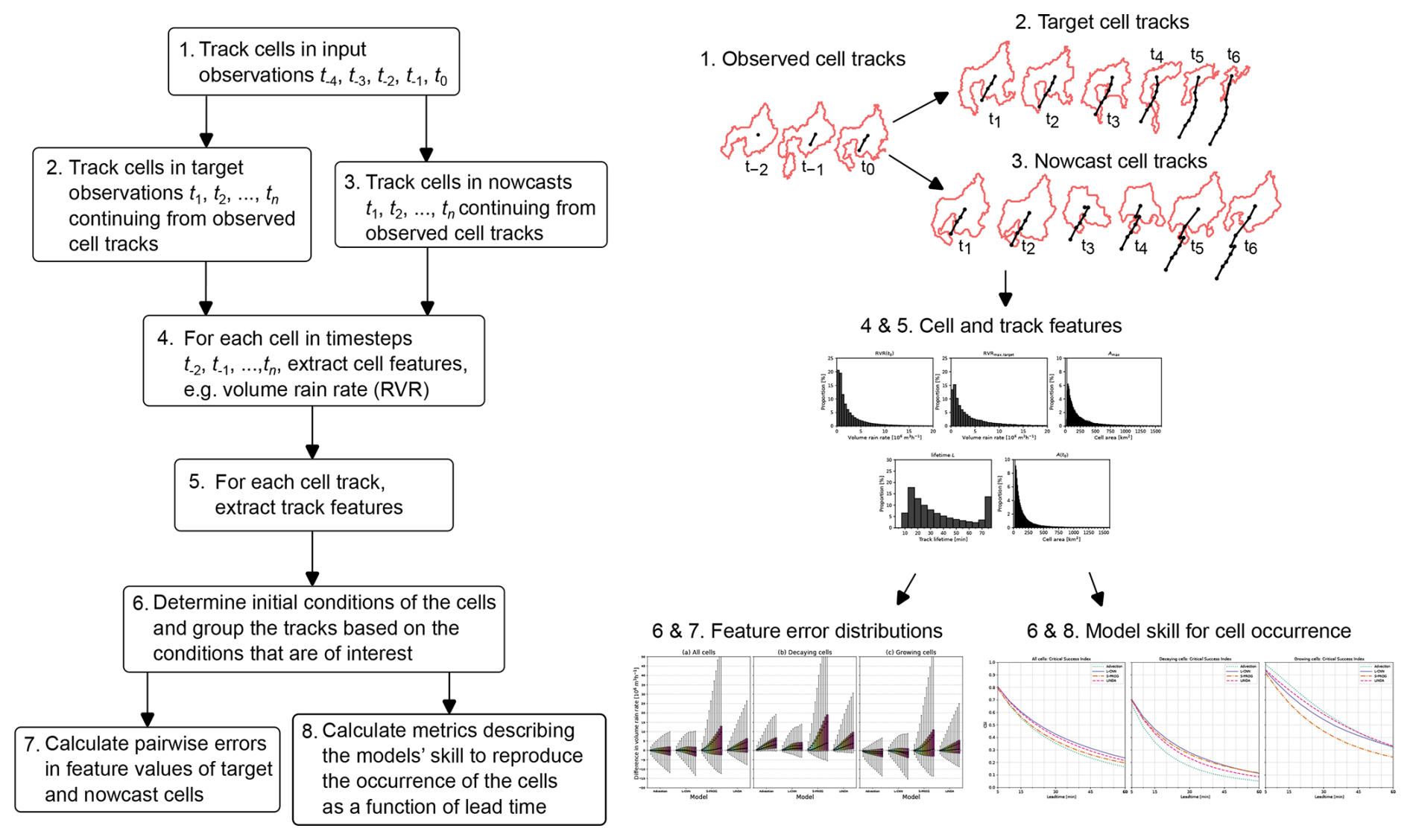
Figure 1 Flowchart of the proposed cell-tracking-based framework for studying nowcasting model skill for convective rainfall. The schematic on the left depicts the outputs of the different steps. The cells are (1) tracked first in the input observations, after which the cell tracks are continued in the (2) target observations and (3) in the nowcasts. After that, features describing (4) the cells and (5) the tracks are extracted from the cells. (6) The cell tracks are then differentiated based on initial conditions of interest, and (7) errors for the feature values and (8) metrics describing the cell occurrence are determined.

Compared with NWP forecasts and reanalysis data, nowcasts computed by extrapolation of weather radar measurements pose additional challenges and possibilities for object-based verification. First, weather radar data often have higher spatial and temporal resolutions. This allows for the identification and tracking of the objects at smaller scales, often resulting in a larger number of identified cells. Second, for most weather-radar-based nowcasting models, the initial state of the nowcast is the last observation. This allows for (1) the comparison of the objects identified in the observations to their counterparts in the nowcasts and (2) the determination of the exact initial state of the objects by tracking them backwards in time. However, in previous nowcasting studies where object-based verification methods have been utilised (e.g. Zahraei et al., 2012; Fox et al., 2016; Li et al., 2018; Wen et al., 2023; Kong et al., 2023; Ji et al., 2023), the methods have been applied separately to each forecast time step.

In this study, we present a cell-tracking-based framework for studying how well the nowcasting models forecast the development of convective cells. An overview of the framework is shown in Fig. 1. In the framework, the convective cells that are identified in the input observations are tracked separately in the target observations and the nowcast fields, and the nowcast cells are compared with the observed cells. We demonstrate the framework using four advection-based models: the advection nowcast, S-PROG (Seed, 2003), LINDA (Pulkkinen et al., 2021), and L-CNN (Lagrangian Convolutional Neural Network; Ritvanen et al., 2023). The aim of the framework presented here is to aid model developers in better understanding the models' ability to predict the development of convective rainfall and to verify whether the development is predicted realistically.

The rest of this article is structured as follows: Sect. 2 describes the data and nowcasting methods that are used in the study; Sect. 3 presents the framework, and Sect. 4 describes the results obtained by applying the framework to the data; and, finally, Sect. 5 concludes the study and discusses the implications of the proposed framework.

2 Data and nowcasting models

2.1 Radar data

The rainfall dataset used in this study is the operational radar-only quantitative precipitation estimation (QPE) product from MeteoSwiss for Switzerland (Germann et al., 2006, 2022). The study domain covered by the rainfall product is shown in Fig. 2. The rainfall product is produced from radar reflectivity observations using the Z–R relation Z=316R^1.5; here, the radar reflectivity Z is in linear units of millimetres to the sixth power per cubic metre, and the rainfall rate R is in units of millimetres per hour (Germann et al., 2006; Joss et al., 1998). The data are further processed to remove ground clutter and non-meteorological echoes, correct for visibility and vertical profile of rainfall, and correct for bias compared to rain gauge measurements (Germann et al., 2006), before being stored in an 8-bit format. Furthermore, the data are saturated at approximately 120 mm h⁻¹ (approximately 56 dBZ).

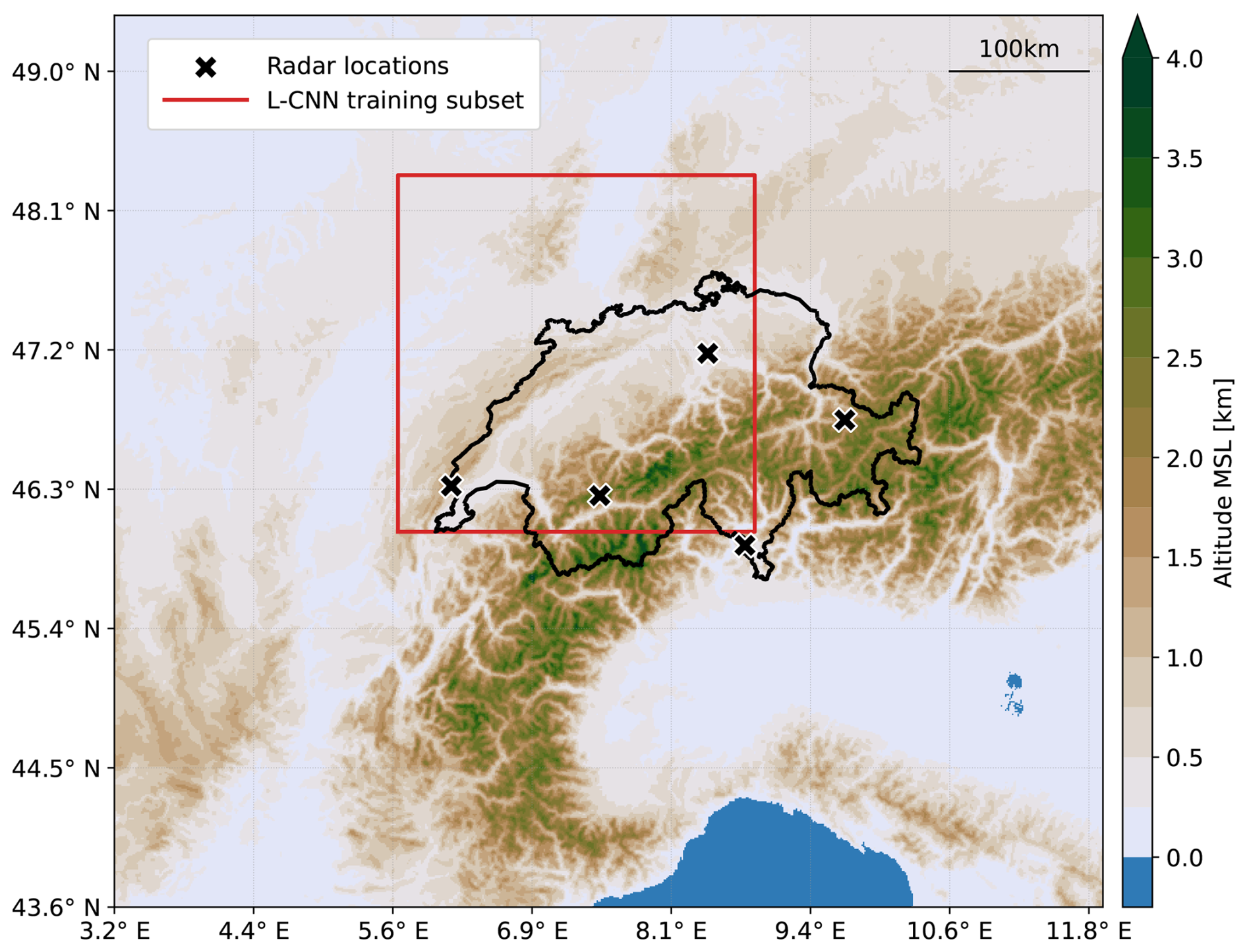
Figure 2 Study domain. The colour indicates the ground altitude in metres above mean sea level (MSL). The black line shows Switzerland's borders. The bounding box used in training the L-CNN model is shown in red, and the black crosses indicate radar locations.

We used data from May to September from the years 2021 to 2023. From these dates, we applied a selection criterion similar to that in Ritvanen et al. (2023). First, we ranked the dates in descending order according to the number of pixels exceeding 1.0 mm h⁻¹ during the day. Second, we selected the 150 first ranked days as the study material. Furthermore, we split this study dataset into training, validation, and test datasets. The training and validation datasets were used to train the L-CNN model (see Sect. 2.2.4), and the test dataset was used to perform the analysis. The data were split by first dividing each day into 6 h blocks. Then, any blocks containing missing data or images with less than 1 % pixels larger than 1.0 mm h⁻¹ were removed. The remaining blocks were then randomly divided into training, validation, and test datasets at a ratio of $\mathrm{6}:\mathrm{1}:\mathrm{5}$, respectively.

The temporal resolution of the data is 5 min, and the spatial resolution is 1 km. The original size of the rainfall fields is 710 pixels × 640 pixels. However, to obtain an image size that is a multiple of 2⁵ in both dimensions, as required by the U-Net component of the L-CNN model (Ritvanen et al., 2023; Ayzel et al., 2020), we removed the first 6 pixels from the left edge, resulting in cropped images of 704 pixels × 640 pixels. For the analysis presented in this study, we generated nowcasts with each model using the cropped images in the test dataset. The nowcasts were created every 5 min for a maximum lead time of 60 min with 5 min time steps.

2.2 Nowcasting models

In this study, four nowcasting models were used: advection nowcast, S-PROG, LINDA, and L-CNN. The models are advection-based, meaning that the motion of rainfall is predicted separately from the temporal evolution of the rainfall. The motion is predicted by extrapolation along a motion field in all four models, but the models differ by how the temporal evolution is predicted in a Lagrangian coordinate system.

2.2.1 Advection nowcast

The advection nowcast model, i.e. Lagrangian persistence nowcast, consists of determining the rainfall motion field from previous rainfall fields and then extrapolating the latest observed rainfall field forward in time using the determined motion field. The motion field v is determined using the Lucas–Kanade optical flow (Lucas and Kanade, 1981; Bouguet, 2001) method implemented in the pysteps library (Pulkkinen et al., 2019b; Germann and Zawadzki, 2002). The motion field is determined using four previous rainfall fields. We used the default settings for the algorithm (Nerini et al., 2023).

The advection nowcast produces no evolution in the rainfall field. However, there may be small distortions in the fields due to the extrapolation method, and the motion field may contain divergence or convergence that warps the rainfall field. As the motion fields in this study are calculated from four input fields, the resulting motion field is expected to be smooth in areas with rainfall, while convergence or divergence is more likely at the edges or areas with less rainfall. Therefore, the impact of distortions due to convergence or divergence is likely small at short lead times, when the predicted rainfall is close to its original position, and becomes larger as the lead time increases.

2.2.2 S-PROG

The S-PROG (Spectral Prognosis; Seed, 2003) nowcast model is based on the assumption that the predictability of rainfall depends on the spatial scale of the rainfall. The S-PROG model is calculated by transforming the input rainfall fields to a Lagrangian coordinate system; decomposing the rainfall field into different spatial scales with cascade decomposition; evolving each cascade separately with a lag-2 autoregressive (AR(2)) model; summing the evolved cascade fields; and, finally, advecting the summed field to the next time step. In this study, a modified version of S-PROG proposed by Pulkkinen et al. (2019a) is used in which AR(2) is applied to the cascade fields in the spectral domain. We used the S-PROG implementation from the pysteps library (Pulkkinen et al., 2019b; Nerini et al., 2023); for more details on the model, refer to Seed (2003), Pulkkinen et al. (2019a) and Pulkkinen et al. (2018).

Owing to the use of AR(2) at multiple spatial scales, the S-PROG model filters out small-scale variations, thereby creating progressively smoother nowcasts. While this improves the skill of the model by filtering out the small-scale variability that has poor predictability, it also leads to the blurring of high reflectivity values, i.e. convective rainfall.

2.2.3 LINDA

The LINDA (Lagrangian Integro-Difference equation model with Autoregression; Pulkkinen et al., 2021) follows a similar approach to the S-PROG model; however, instead of an AR(2) model applied to cascade levels in the spectral domain, the dependence of the predictability of the field on the spatial scale is modelled with a Gaussian convolution-based model and the evolution of the rainfall field through an autoregressive integrated process (ARI(1, 1)). We used the deterministic LINDA model implementation from the pysteps library (Pulkkinen et al., 2019b; Nerini et al., 2023).

The LINDA model implementation allows one to fit the parameters of the convolution models and ARI processes separately either to each detected rain cell or to the full rainfall field domain. Although the first approach might perform slightly better for convective rainfall, the difference in performance between the two approaches is not significant (Pulkkinen et al., 2021), and the first approach is much more computationally expensive than the latter. Therefore, in this study, we used the latter approach, in which the parameters are optimised for the full domain. Note that the ARI process is still applied separately to each cell.

In previous studies, LINDA has been found to perform better for heavy rainfall than S-PROG (Pulkkinen et al., 2021) or RainNet (Ayzel et al., 2020), a U-Net convolutional neural network (CNN) model (Ritvanen et al., 2023). A visual inspection of the nowcasts produced by LINDA (Fig. 3) shows that, although it is able to maintain higher rain rates better than S-PROG, LINDA tends to spread the high-intensity areas, leading to blurring in the nowcasts.

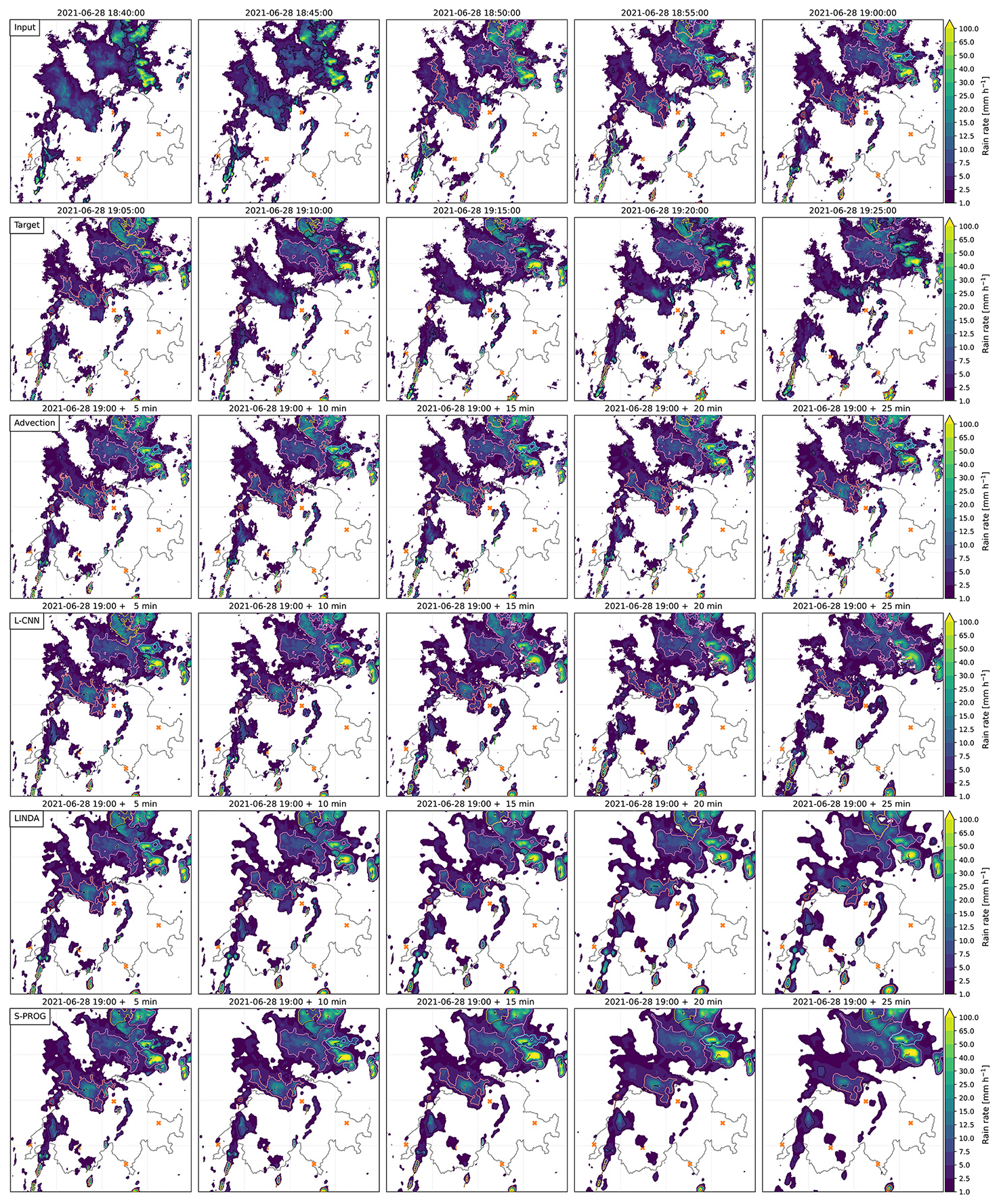
Figure 3 Example of cell-tracking results at 19:00 UTC on 28 June 2021. The panels show the rain rate fields for observations, target observations, and nowcasts. The convective cells identified at that time are plotted in each panel. The cells included in the analysis are shown using coloured contours, with each colour indicating cells belonging to the same track. For each cell track, the cell centroid locations are shown using coloured triangles on top of the black tracks. Cells that were not matched to any track existing at the nowcast creation time step are shown as black contours. The orange crosses indicate the radar locations. Note that panels are zoomed in and do not show the entire domain demonstrated in Fig. 2.

2.2.4 L-CNN

The L-CNN (Lagrangian Convolutional Neural Network; Ritvanen et al., 2023) applies a U-Net neural network to the temporal difference in rain rate fields. The approach is similar to that of LINDA; however, instead of the ARI and convolution models, the U-Net component is used to model the evolution of the temporal difference in rain rate in the Lagrangian coordinates. In a previous study (Ritvanen et al., 2023), this was found to improve, for example, the equitable threat score at short lead times and high rain rate thresholds.

The U-Net component of the L-CNN model was trained using a procedure similar to that in Ritvanen et al. (2023). As described in Sect. 2.1, the model was trained using the training dataset split, and the convergence of the training was determined using the validation dataset. To speed up the training procedure, we chose a subset of 256 pixels × 256 pixels from the Swiss rainfall product (see Fig. 2). The L-CNN model was implemented with the PyTorch (Paszke et al., 2019) and PyTorch Lightning (Falcon and The PyTorch Lightning team, 2019) libraries, and the implementation is available online (Ritvanen, 2024a). Training was performed using a compute node with eight NVIDIA V100 GPUs made available by the Swiss National Supercomputing Centre (CSCS).

3 Cell-tracking-based verification framework

In the following sections, we describe the convective cell-tracking-based verification framework presented in this study. For the purposes of this study, we define convective cells as all cells that are identified with the contour-based cell identification algorithm where the contours are extracted with a threshold of 35 dBZ, without any further separation based on cell type, and the rainfall inside these cells is considered convective rainfall. The framework (Fig. 1) consists of the following steps:

1. Identify and track the observed cells in the input observations at time steps $t_{-\mathrm{4}},\mathrm{\dots },t_{\mathrm{0}}$.

2. Continuing from the cell tracks in the input observations, track the observed cells in the target observations at time steps $t_{\mathrm{1}},\mathrm{\dots },t_n$.

3. Continuing from the cell tracks in the input observations, track the cells in the nowcast fields at time steps $t_{\mathrm{1}},\mathrm{\dots },t_n$.

4. Extract features of all detected cells.

5. Extract track features separately for the cell tracks in target observations and nowcasts.

6. Determine cell track classification into decaying or growing at the nowcast creation time separately for the target and nowcast cell tracks.

7. Calculate error distributions between the feature values in the target and nowcast cells.

8. Calculate metrics describing, for example, the models' ability to reproduce the existence of cells as a function of lead time.

The cell identification and tracking algorithms should be selected to identify and track the cells in a way that is meaningful for the purposes for which the nowcasts are used. Additionally, the algorithms should be able to identify and track the cells in the nowcasts where, depending on the model, the structure of rainfall can vary significantly from the observations. In this study, convective cell identification and tracking were performed using the Thunderstorm Detection and Tracking (T-DaTing) algorithm (Feldmann et al., 2021) implemented in the pysteps library (pySTEPS developers, 2023) and inspired by the thunderstorm radar tracking (TRT) algorithm presented in Hering et al. (2004). The implementation of the cell identification and tracking algorithms is available online at https://doi.org/10.5281/zenodo.11242613 (Nerini et al., 2024).

3.1 Convective cell identification

Convective cells are identified from the rainfall fields in logarithmic radar reflectivity units (dBZ). Because our data are otherwise processed as rain rate in units of millimetres per hour, we first transform the fields into radar reflectivity using the formula Z=316R^1.5, where R is the rain rate and Z is the radar reflectivity in linear units of millimetres to the sixth power per cubic metre (Joss et al., 1998; Germann et al., 2006).

After that, we employ the cell identification algorithm (Hering et al., 2004; Feldmann et al., 2021) implemented in the pysteps library (Pulkkinen et al., 2019b). The algorithm begins by discarding all pixels in the rainfall fields below the minimum reflectivity threshold Z_min. From the remaining connected pixel areas, any areas that have peak values less than the peak reflectivity Z_p or smaller than the minimum area threshold A_min are discarded. Subsequently, any reflectivity value above the maximum reflectivity threshold Z_max is saturated to that value, and a local maximum detection algorithm (van der Walt et al., 2014) is used to find the local maxima inside each connected area. The local maxima values are then counted as separate cells if (i) the path of least change between them decreases by at least ΔZ and (ii) the maxima are located at least d_min apart. Cells within the same connected area are separated using an inverted watershed algorithm (Beucher and Lantuejoul, 1979; van der Walt et al., 2014).

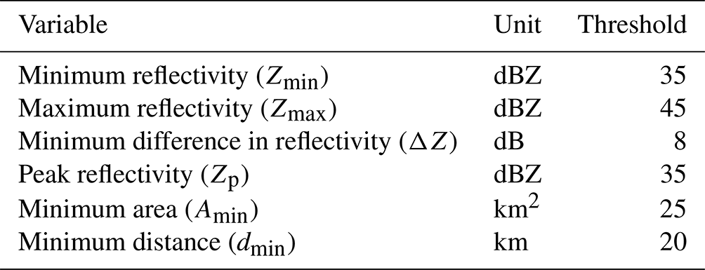
As we will compare the features of the identified cells, the selected cell identification method and parameters can potentially impact the results. Table 1 lists the algorithm parameter values used in this study. For the minimum reflectivity Z_min and the maximum reflectivity Z_max, the pysteps library default values were used. The peak reflectivity threshold was lowered to Z_p=35 dBZ, i.e. equal to the cell detection threshold, as we do not want to discard any cells even if the peak reflectivity inside them would not exceed 35 dBZ. The minimum area threshold was set to A_min=25 km² to also detect smaller cells compared with the work presented by Feldmann et al. (2021), who used a threshold of 50 km², as smaller cells are of higher interest to this work (see Sect. 4.1). Note that a lower bound for the cell area is required to remove clutter, but the selected value is arbitrary. Finally, the minimum difference in reflectivity between maxima to be considered separate cells was set to 8 dB, while the minimum distance was set to 20 km. The selection of these parameters was not as straightforward, as their values cannot be directly linked to the qualities of the identified cells, and because of the algorithm implementation in the pysteps package, the parameter values impact each other and cannot be selected independently. Instead, the values were selected based on an iterative manual process of comparing the identified cells and cell tracks with different parameter combinations. From the tested parameter combinations, the selected values produced cell tracks with the least “spurious” splits or merges, i.e. situations where large cells with multiple close-by maxima would be split to multiple cells in a way that is inconsistent between consecutive time steps. Furthermore, a comparison of the analysis results showed few differences between different parameter combinations.

Table 1 Parameters used for identifying convective cells. The notation follows the algorithm description given in Feldmann et al. (2021).

3.2 Convective cell tracking

After the convective cells have been identified, cell tracks are established using the tracking algorithm (Hering et al., 2004; Feldmann et al., 2021) by matching them with the cells observed at the next time step. First, the motion of the cells is determined from the current and two previous input rainfall fields using the Lucas–Kanade optical flow algorithm (Lucas and Kanade, 1981; Bouguet, 2001; Pulkkinen et al., 2019b). The cells are then propagated to the next time step along the resulting motion field and compared to the cells observed in the current time step. Any two cells with an overlap greater than 40 % are considered the same cell and are assigned the same identifier. If multiple cells from the previous time step overlap by more than 10 % with the same cell, the cell is considered merged; in this case, the identifier of the cell with the largest overlap from the previous time step is assigned to the new cell, and all other cells are considered decayed if they were not matched with any other cell in the current time step. If one cell overlaps more than 10 % with multiple cells at the next time step, the cell track is considered split, in which case the new cell with the largest overlap inherits the identifier of the previous cell, and the cells with smaller overlaps obtain new identifiers.

The result of the tracking algorithm is a list of cell tracks. Because we used two previous rainfall fields to determine the motion of the cells, we only obtain cell tracks for time steps $t_{-\mathrm{2}},t_{-\mathrm{1}}$, and t₀ when using input observations from time steps t₋₄, …, t₀. For the target observations and nowcasts, we continue the tracking from the cells tracked in the input observations and discard any tracks and cells that are not a continuation of these input observation tracks.

In the analysis presented in Sect. 4, we use the cell tracks where we consider only the “most representative” cell track; thus, splits and merges in the cell tracks are ignored and the cells with the largest overlap are considered the continuation of the track, as described above. However, because the splits and merges in the cell tracks influence the observed life cycle of the cells and can therefore potentially impact the analysis, it is important to investigate the extent to which the results are impacted. To this end, we also repeated the analysis using a dataset in which all cell tracks with splits or merges in the input or output observations were removed. In this dataset, all tracks with cells that were the result of a merge of multiple cells, cells that split into multiple cells, or cells that merge with some other cell at the next time step, during either the input or target observations, were excluded. Additionally, all corresponding nowcast cell tracks, i.e. nowcast tracks starting from the input cell track of any excluded observed cell track, were also excluded. The relevant results from this dataset are provided in the Supplement, and we discuss the differences in Sect. 4.5.

While the proposed approach for considering the splits and merges, along with how the most representative cell track is defined, is elementary and other possible approaches and definitions exist, we also note that the nowcasting models used in this study are not expected to reproduce the splits and merges correctly, and the blurring occurring in the nowcasts will impact how and at what time step the splits and merges are identified in the nowcasts. Additionally, the number of splits and merges in the dataset is small (see Sect. 4.5). Therefore, even though this approach might not suffice for statistical analysis of, for example, convective cell life cycles, for the purposes of this study, i.e. a comparative analysis of the selected nowcasting models, the proposed approach is sufficient. A more detailed analysis with more complicated definitions for the most representative cell track, for example, by also including the decayed branches of merged cell tracks in the analysis and analysing how accurately the models reproduce the splits and merges, would be necessary and of interest for models that are expected to reproduce such development in convective cells. Such analysis would most likely also require using a cell-tracking algorithm with a more advanced processing of splits and merges. For now, we consider a more detailed analysis to be outside the scope of this study.

3.3 Convective cell and track features

For each cell in the observations and nowcasts, we determine the following features to describe the cell:

• Volume rain rate (RVR). RVR represents the integrated rain rate over the cell area at a given time step (in m³ h⁻¹). The definition follows what was used, for example, by Rosenfeld (1987), Hu et al. (2019), and Feng et al. (2018).

• Cell area (A). A denotes the area (in m²) of the cell at a given time step as identified from the rainfall field.

• Mean rain rate (R_avg). R_avg is the mean rain rate inside the cell at a given time step (in mm h⁻¹).

In addition to the features that describe each cell, we determine the following features describing the cell tracks:

• Lifetime (L). L denotes the observed lifetime (in minutes) of the cell track, i.e. the number of time steps that the track exists in the input and target observations multiplied by the time step (5 min). Note that, as we only obtain cell tracks at 3 time steps before the nowcast is created and 12 time steps after, the lifetime is saturated to 75 min.

• Maximum observed cell area (A_max). A_max is the maximum observed cell area (in m²) for a cell track during the time steps where the track exists in the input and target observations.

Only the cell and track features used in the analysis presented in Sect. 4 are described here. However, depending on the investigated nowcasting models, other features may also be of interest. For example, we do not consider the location of the cells. For advection-based nowcasting models, the error in cell location predicted by the models, defined, for example, through the error in cell centroid location between observed and corresponding nowcast cells, would consist of error in the predicted motion of the cell, i.e. the error in the motion field, and error in the centroid location inside the cell caused by the cell shape. As the models used in this study use the same motion field and extrapolation method, the first component of the errors would be the same; therefore, any differences between the cell location errors would be small and depend mainly on the cell shape, which would make the location errors difficult to interpret. However, for models in which the cell motion is affected by different factors, the location error can be of interest. Another potentially interesting feature is the maximum rain rate inside a cell; however, for our data, this value is saturated at approximately 120 mm h⁻¹ because of the saturation in the original rainfall product, which causes bias in the errors in the maximum rainfall rate.

The aim of the proposed framework is to investigate the ability of the models to predict the development of convective rainfall and the impact of the initial stage of the convective cell. The development of the cell during the nowcast period depends on the stage of the cell when the nowcast is created, i.e. whether the cell is growing or decaying. To quantify this, we define a status for each cell track at the nowcast creation time. The status is determined using the derivative of the cell volume rain rate at the nowcast creation time t₀, i.e. dRVR_obs(t₀). The derivative is estimated using at most the values at $t_{-\mathrm{2}},\mathrm{\dots },t_{\mathrm{2}}$, of which three values are required to exist for the derivative to be defined. The track status is classified as growing if dRVR_obs(t₀)>0. Conversely, the track status is classified as decaying if dRVR_obs(t₀)<0 or if the track exists at t₀ but not at t₁. In addition to the observations, we determine the status of the cell tracks similarly in the nowcast rainfall fields using dRVR_ncst(t₀), which is calculated by replacing the RVR values from target observations with the predicted RVR values in the derivative estimation.

3.4 Evaluation of model skill in reproducing convective cell development

The aim of the proposed framework is to study how accurately the nowcasting models reproduce convective cell development. To study this question, we consider the cell tracks (Sect. 3.2) that exist when the nowcast is created at t₀ and compare the cells in these tracks in the nowcasts to the cells in the corresponding tracks in the target observations. In the results presented later, only the most representative cell track was considered, as described in Sect. 3.2. While this approach discards all cells in tracks newly initiated after t₀ and, therefore, does not allow the study of new cell formation, it permits us to study the impact of input observations on how well the model reproduces convective cell development. As a model should be able to predict the evolution of cells that it has seen in the input observations better than that of cells that develop later, the results of this analysis can be considered to be the upper limit for model skill in reproducing the development of cells that do not yet exist at the time of nowcast creation.

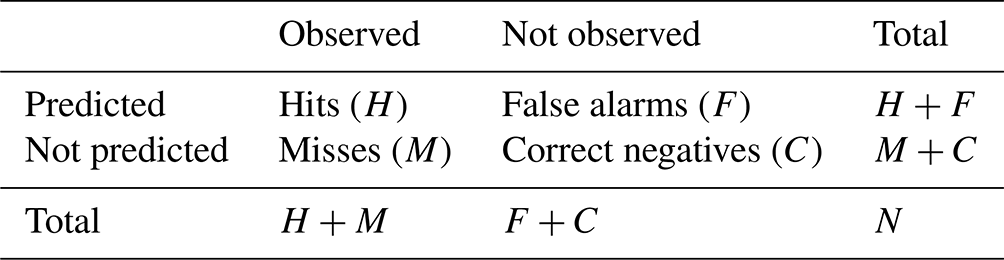
Using this approach, we define the contingency table (Table 2) elements as follows.

• Hits (H). H represents cells that exist in both target observations and the nowcast.

• Misses (M). M represents cells that exist in target observations but not in the nowcast.

• False alarms (F). F represents cells that exist in the nowcast but not in target observations.

• Correct negatives (C). C represents cell tracks that existed in the input observations at t₀ and do not exist in target observations or the nowcast.

Metrics calculated using these definitions for the contingency table elements describe the skill of the model in reproducing the cell occurrence given that the corresponding cell track existed in the input observations. From these values, we calculate (as a function of the lead time) the critical success index (CSI), probability of detection (POD), false alarm ratio (FAR), and frequency bias (BIAS) metrics, which are defined as follows:

$$\begin{array}{}\text{(1)}& {\displaystyle }\text{CSI}={\displaystyle \frac{H}{H+M+F}},\text{(2)}& {\displaystyle }\text{POD}={\displaystyle \frac{H}{H+M}},\text{(3)}& {\displaystyle }\text{FAR}={\displaystyle \frac{F}{H+F}},\text{(4)}& {\displaystyle }\text{BIAS}={\displaystyle \frac{H+F}{H+M}}.\end{array}$$

The BIAS values range from 0 to ∞, with 1 indicating a perfect score. The other metric values are between 0 and 1; for CSI and POD, the optimal value is 1, whereas the optimal value is 0 for FAR.

Table 2 Contingency table for binary forecasts.

This approach allows us to define the concept of correct negatives. However, because the dataset only includes cell tracks that exist at the nowcast creation time, the number of correct negatives will be very small compared with the other categories, especially at short lead times. This can lead to unintuitive score values for metrics that utilise correct negatives, such as the equitable threat score, compared with more balanced datasets. Therefore, we selected to use only metrics that are defined without correct negatives.

Another point of interest is how well the models reproduce the cell track classification into a growing or decaying track that describes the initial predicted development of the cell. In the nowcasts, the cell track classification is affected, in addition to the input observations, by the volume rain rate of the nowcast cell in the first two lead time steps; therefore, correct classification would indicate that the model predicts the initial cell development similar to what was observed for that cell.

To study this, we define the cell track classification as a two-category classification problem. For example, in this case a hit (H) for the class decay (growth) would be a cell track whose status is classified as decaying (growing) in both observations and the nowcast. The definitions of misses (M), false alarms (F), and correct negatives (C) follow similarly. Using these, we can estimate the goodness of the classification with different metrics. In addition to the CSI (Eq. 1), POD (Eq. 2), FAR (Eq. 3), and BIAS (Eq. 4), which are calculated separately for both classes, we also use the equitable threat score (ETS; Schaefer, 1990) and the Gerrity score (GS; Gerrity, 1992). The ETS measures the fraction of correctly predicted events accounting for hits due to random chance and is defined as follows:

$$\begin{array}{}\text{(5)}& \text{ETS}={\displaystyle \frac{H-H_{\mathrm{r}}}{H+M+F-H_{\mathrm{r}}}},\end{array}$$

where

$$\begin{array}{}\text{(6)}& H_{\mathrm{r}}={\displaystyle \frac{(H+M)(H+F)}{N}}\end{array}$$

and N is the total number of observation–forecast pairs. ETS obtains values from $-\mathrm{1}/\mathrm{3}$ to 1, with negative values indicating worse forecast skill than random chance, 0 indicating similar forecast skill as random chance, and 1 indicating a perfect forecast. Note that, in this two-category definition, the ETS value is symmetric between the classes. The Gerrity score is defined as follows:

$$\begin{array}{}\text{(7)}& \text{GS}={\displaystyle \frac{\mathrm{1}}{N}}\sum _{i=\mathrm{1}}^K\sum _{j=\mathrm{1}}^{K}n(F_j,O_i)s_{\mathit{ij}},\end{array}$$

Here, N is the total number of observation–forecast pairs, K is the number of classes (i.e. here K=2), n(F_j,O_i) is the number of forecasts in class j that had observations in class i, and the elements of the scoring matrix s_ij are defined as follows:

$$\begin{array}{}\text{(8)}& {\displaystyle }\begin{array}{rl}& s_{ii}={\displaystyle \frac{\mathrm{1}}{K-\mathrm{1}}}\left(\sum _{r=\mathrm{1}}^{i-\mathrm{1}}{a}_r^{-\mathrm{1}}+\sum _{r=\mathrm{1}}^{K-\mathrm{1}}{a}_r\right),\\ & s_{\mathit{ij}}=s_{\mathit{ji}}={\displaystyle \frac{\mathrm{1}}{K-\mathrm{1}}}\left(\sum _{r=\mathrm{1}}^{i-\mathrm{1}}{a}_r^{-\mathrm{1}}-(j-i)+\sum _{r=\mathrm{1}}^{K-\mathrm{1}}{a}_r\right),\\ & a_i=\left(\mathrm{1}-\sum _{r=\mathrm{1}}^i{p}_r\right)/\sum _{r=\mathrm{1}}^i{p}_r,\end{array}\end{array}$$

where p_i is the observed frequency of class i. The Gerrity score describes the accuracy of the forecast for predicting the correct class considering random chance, and it obtains values from −1 to 1, with 1 indicating a perfect score.

In addition to the occurrence of convective cells, we are also interested in how accurately different cell and track features are reproduced in the nowcast. To study this, for each pair i of cells in the nowcast and target observations for each lead time t, we calculate the difference in the feature values as follows:

$$\begin{array}{}\text{(9)}& \mathrm{\Delta }{x}_i\left(t\right)=x_{i,\text{ncst}}\left(t\right)-x_{i,\text{target}}\left(t\right),\end{array}$$

where x_i,ncst(t) is the feature value obtained from the cell from the nowcast and x_i,target(t) is the feature value obtained for the corresponding cell in the target observations. If one of the cells does not exist, i.e. the track has died either in the target observations or the nowcast (or both), the cell pair is discarded. From the values Δx_i(t), we estimate the mean and median values, i.e. the mean and median errors in feature values, and plot the distributions per lead time and model.

Additionally, we measure the overall predictive capability of the models using the root-mean-square error (RMSE) of the cell volume rain rate, calculated by also considering the cases in which either the target observation cell no longer exists but the nowcast cell exists (false alarm) or the target cell exists but the nowcast cell does not (miss). In these cases, the volume rain rate of the non-existent cell is taken as 0. Calculated in this way, the error reflects both the model skill in reproducing the cell feature values and penalises the models' inability to reproduce the life cycle of the cells. The volume rain rate is selected for this error over the other features, as this feature describes the total rainfall produced by the cell, combining the impact of the cell area and the distribution of rainfall inside the cell. The RMSE is defined as follows:

$$\begin{array}{}\text{(10)}& \text{RMSE}=\sqrt{{\displaystyle \frac{\mathrm{1}}{n}}\sum _{i=\mathrm{1}}^n({\text{RVR}}_{i,\text{target}}-{\text{RVR}}_{i,\text{ncst}}{)}^{\mathrm{2}}},\end{array}$$

where RVR_i,target and RVR_i,ncst are the volume rain rate values of the ith pair of corresponding target and nowcast cells, respectively.

3.5 Evaluation of model skill in reproducing convective cell occurrence

The approach described above does not include information on the formation of new cells or the death of existing cells that are not part of the cell tracks included in the dataset. Rather, this needs to be studied separately. To study the occurrence of the convective cells in the nowcasts, we define it as a binary classification problem: can the convective cell identified in the nowcast be matched to an identified cell in the target observations? A similar approach has been used to verify cell-tracking algorithms (e.g. Dixon and Wiener, 1993; Zan et al., 2019; Zhang et al., 2021) and recently for nowcast model evaluation (Wen et al., 2023). Compared with Wen et al. (2023), we evaluate the metrics separately at each lead time, not averaged over all lead times, as it is expected that the model skill for reproducing cell occurrence should decrease as the lead time increases.

To study how well the models reproduce cell occurrence, we consider the cells that have been identified in the target observations and nowcasts, as described in Sect. 3.1, separately at each lead time step. Note that the cell-tracking results are not used here; therefore, all identified cells are considered. Following Wen et al. (2023), the cells in the target observations are matched to the cells in the nowcasts using the Hungarian algorithm (Kuhn, 1955; Crouse, 2016; Virtanen et al., 2020) based on the distance between the cell centroid locations. The result is the combination of matches between the cells that minimises the total sum of the distances between the matched cell centroids. If any match has a distance greater than 20 km, it is considered invalid and the cells unmatched.

The results of this analysis are a set of matched and unmatched cells between the target observations and nowcasts. Next, we define the contingency table elements for this problem. Note that, as the problem setting is different from Sect. 3.4, the contingency table (Table 2) elements also have different definitions; here, for the cell matching without tracking, the elements are defined at each time step after t₀ as follows:

• Hits (H). H represents cells that are matched between target observations and nowcast at that time step.

• Misses (M). M represents cells that exist in target observations at that time step but are not matched to any cell in the nowcast.

• False alarms (F). F represents cells that exist in nowcast at that time step but are not matched to any cell in the target observation.

Note that when defining the problem in this way, the category of correct negatives has no definition, as we cannot count cells that do not exist in the target observations or the nowcasts.

The metrics calculated from the contingency table elements are defined in the same manner as in Sect. 3.4 (Eqs. 1–3). However, as the definitions of the contingency table elements differ, the metrics have different interpretations that should not be confused. Here, the metrics describe how well the models reproduce the convective cells that were identified in the observations, without including any information about the cell track history. For a contingency table defined as above, we would expect that a model's increased ability to create new convective rain would result in an increased CSI and POD, especially at longer lead times. However, if the model creates too many cells compared with observations, the FAR should increase, indicating decreased skill. Similarly, if the model suppresses cells similar to the observations, the FAR should decrease.

4 Results

4.1 Cell track dataset statistics and example case

Figure 4 shows (separately for all cell tracks, decaying cell tracks, and growing cell tracks) the distributions of cell volume rain rate (Fig. 4a–c) and area (Fig. 4d–f) at the nowcast creation time t₀, the maximum observed cell area (Fig. 4g–i), and the observed track lifetime (Fig. 4j–l). The distributions of the observed cell track lifetime indicate that the division of the cell tracks into decaying or growing tracks is successful: most decaying tracks have an observed lifetime of less than 30 min (note that the lifetime only accounts for the observed time steps), whereas the lifetime distribution of the growing tracks has fewer values at short lifetimes and a high peak at 75 min, which contains lifetimes of 75 min or longer. The distribution of the RVR(t₀) for the decaying cell tracks (Fig. 4b) shows more cells with small volume rain rates than the growing cell tracks (Fig. 4c). A similar behaviour is observed for cell area A(t₀) (Fig. 4h and i). This is mostly explained by the fact that the decaying category includes cells that exist at t₀ but not at t₁, which also explains the larger number of cells in the decaying category than that in the growing tracks category.

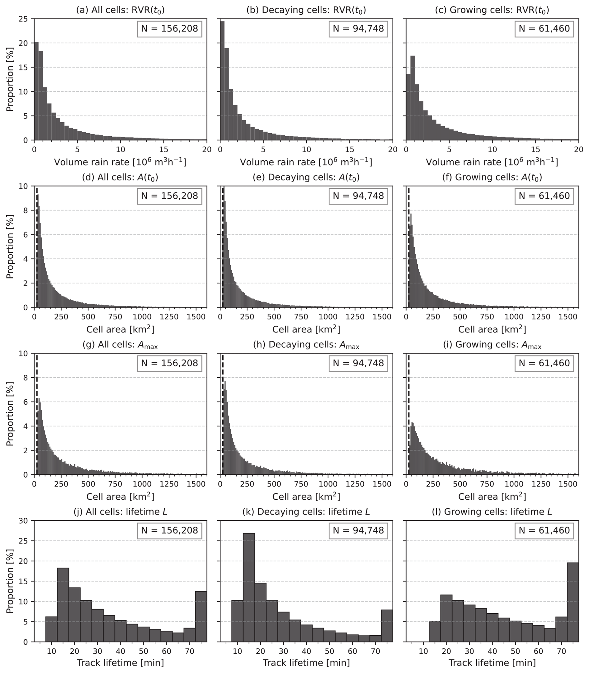
Figure 4 Histograms of cell and track feature values. The panels show (a–c) the volume rain rate at the last observed time step t₀; (d–f) the cell area at t₀; (h, i) the maximum observed cell area; and (j–l) the observed cell track lifetime. Histograms are shown for all cells (a, d, g), decaying cells (b, e, h), and growing cells (c, f, i). The value in each panel indicates the number of cells in the histogram. In the cell area histograms (d–i), the vertical dashed line indicates the minimum cell area threshold of 25 km².

Figure 3 shows an example of the nowcasts and convective cell tracking at 19:00 UTC on 28 June 2021 . The panels show the input observations in the first row, the target observations in the second row, and the nowcast rainfall fields in the consecutive rows. Each panel shows the cells identified from the fields, with coloured contours indicating cells that are part of the tracks existing at t₀, and black contours indicating cells that are not part of such tracks.

The nowcasts in Fig. 3 demonstrate the features of the different models. For example, the blurring occurring in LINDA and S-PROG as the lead time increases is visible in both the smoothing of the rainfall field and the subsequent smoothing of the cell contours. Additionally, S-PROG shows a clear loss of small cells compared with the other models. While L-CNN does not smooth the nowcast fields as much, it creates much more local decay, which results in uneven cell contour shapes that are visible, for example, in the cells in the bottom right of the panels.

The case has several small cells that are tracked visually consistently in the input and target observations, for example, in the bottom half of the panels. However, the large cells in the top-right quadrant are split into several cells at certain time steps. Such large cells pose an issue to the identification algorithm because they tend to split “spuriously” into multiple cells if they contain multiple local maxima, as discussed in Sect. 3.1. The selected cell identification algorithm parameters aim to reduce the number of these spurious splits and merges; however, some will still remain in the dataset.

While larger cells are important for nowcasting applications owing to their large hazard potential, we aim (for several reasons) to focus on the smaller cells in the results presented here. First, a majority of the cells in the dataset are small; approximately 88 % of the cells at the nowcast creation time t₀ have an area smaller than 500 km² (Fig. 4d). Second, large convective cells are usually formed of several smaller convective cores, and accurate nowcasting of large cells requires accurate nowcasting of the smaller convective cores. For the models used in this study, the nowcast skill for these convective cores can reasonably be assumed to be similar to that of the individual smaller convective cells. Finally, for large cells, the impact of dislocation error in the pixel-by-pixel verification metrics is smaller than that for small cells; therefore, the large cells would be better represented in these verification metrics. As a result, large cells are a less intriguing research focus for the proposed framework compared with small cells.

Note that the statistics and results presented here describe convective cells, as they were defined to include radar reflectivities above 35 dBZ, detected from the rainfall product used in the study. Using a different cell identification and tracking methodology or another data product would most likely affect the statistics. Because the data used here are from the Swiss radar network, the climatology of convective rainfall and the convective cells is impacted by orography, for example, the Alps; as such, the statistics of the convective cells might be different compared with other locations. However, because our aim is to investigate the performance of the nowcasting models, the statistics of the cell features are mainly used in interpreting the results, and a detailed investigation of the cell statistics themselves is outside the scope of this study.

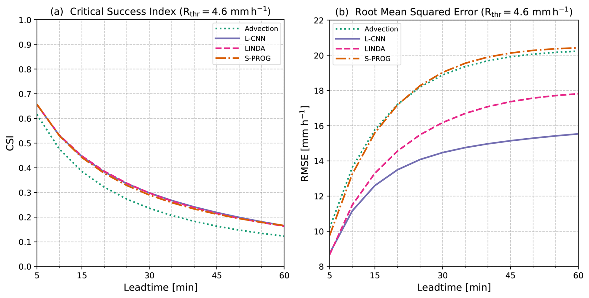
Figure 5 (a) Critical success index (CSI) and (b) root-mean-square error (RMSE) calculated from the nowcasts in a pixel-by-pixel manner. The metrics are conditioned on a threshold of 4.6 mm h⁻¹.

4.2 Model skill shown by pixel-by-pixel metrics

The common approach to verifying radar-based rainfall nowcasting models is using metrics calculated in a pixel-by-pixel manner, either contingency-based metrics, such as the critical success index (CSI), or distance-based error metrics, such as the root-mean-square error (RMSE). Figure 5 shows the CSI and RMSE calculated for the models in this study. Both metrics are conditioned on a threshold of 4.6 mm h⁻¹ (corresponding to 35 dBZ, i.e. the cell identification threshold used in the study). For the CSI, this means that pixel values below the threshold are considered “no” events, whereas pixel values at and above the threshold are “yes” events for the contingency table calculation. For the RMSE, the conditioning means that pixels for which both the predicted and observed value are below the threshold are excluded from the error calculation.

The metrics calculated in a pixel-by-pixel manner provide an overview of the model skill. In our data, the L-CNN, LINDA, and S-PROG models have almost exactly the same performance with respect to the CSI, whereas the advection nowcast performs significantly worse. For the RMSE, the models have more differences, with L-CNN having the smallest error and S-PROG and the advection nowcast having similar error. Note that LINDA and L-CNN aim to minimise the RMSE between the observations and nowcasts leading to smaller RMSE values than for the advection nowcast and S-PROG. Thus, a large part of the RMSE differences can be explained by the varying efficacy of the loss functions in the models, which makes the comparison of the RMSE (or any error metric based on the L2-norm) unfair. Especially in ML models, using a loss function that aims to minimise the prediction error using some loss that does not aim to minimise the L2-norm of the dataset can lead to different trends in L2 errors, while maintaining similar skill with respect to the CSI.

Based on these metrics, one might conclude that the L-CNN model has the best performance and the smallest error in rainfall at the 4.6 mm h⁻¹ (35 dBZ) threshold, with LINDA and S-PROG having similar skill in predicting the exceedance of rainfall at this threshold but with larger errors. Note that any arbitrary threshold gives only a snapshot of the models performance. In this case, for CSI, increasing the threshold decreases the metric values overall (see Fig. S9); relatively, the performance of S-PROG decreases gradually to a level similar to the advection nowcast, while L-CNN and LINDA perform similarly to each other at every threshold. For the RMSE (Fig. S10), increasing the threshold reduces the relative difference between L-CNN and LINDA; the advection nowcast and S-PROG remain similar. However, these metrics, even calculated at multiple thresholds, do not differentiate between various aspects of the models' skill, e.g. whether the models predict the intensity, location, or distribution of heavy rainfall well. Furthermore, the metrics are unable to describe if the model skill depends on the type of rainfall, e.g. if the model is better at predicting decaying than growing rainfall.

4.3 Model skill in reproducing cell development

The main aim of the proposed cell-tracking-based framework is to study how accurately the nowcasting models reproduce the development of the identified cells. We measure the comprehensive model skill with the RMSE of the cell volume rain rate, shown in Fig. 6. In the RMSE calculation, cells that do not exist in the target observations but exist in the nowcast, or vice versa, are considered zero values. That is, in addition to incorrectly predicted cell volume rain rates, the model is also penalised for cell tracks that decay too fast or slow.

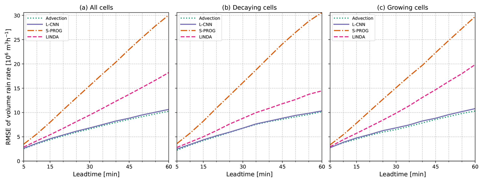
Figure 6 Root-mean-square error (RMSE) of the cell volume rain rate for (a) all cell tracks, (b) decaying cell tracks, and (c) growing cell tracks. The error has been calculated so that the volume rain rate of non-existing cells in either the target observations or the nowcasts is considered to be 0. Cell pairs where neither exists were excluded.

The RMSE is shown separately for all cell tracks, decaying cell tracks, and growing cell tracks. Overall, L-CNN and the advection nowcast have the smallest errors, S-PROG has the largest error, and LINDA falls between the other models. All models show slightly smaller errors for decaying cell tracks, indicating better predictive skill for decaying cell tracks compared with growing tracks. The difference is the largest for LINDA. The impact of various factors to the model skill is studied further in the following sections by separately examining the model skill for predicting the occurrence of the cells and the feature values of the cells.

Compared to the RMSE calculated in a pixel-by-pixel manner (Fig. 5), the major difference in relative errors between the models is the advection nowcast that has significantly smaller error in the cell-based RMSE. As this error metric does not penalise location errors and the lead times are relatively short, the advection nowcast has small errors, but when the RMSE is calculated in a pixel-by-pixel manner and, thus, location error is penalised, the errors are larger. Another difference between the RMSE values is that the error values in the pixel-by-pixel RMSE (Fig. 5) increase sharply at short lead times and plateau as the lead time increases, whereas the cell-based RMSE (Fig. 6) increases linearly. In the pixel-by-pixel RMSE, the sharp increase at short lead times is mostly caused by location error. Contrarily, in the cell-based RMSE, the impact of incorrectly predicted cell existence increases as the lead time increases.

4.3.1 Cell existence in tracks

We examine the models' ability to reproduce convective cell development by first focusing on how well the models are able to reproduce the existence of cell tracks. Figure 7 shows the number of cells tracked per lead time and model. The track counts are shown for the entire dataset (Fig. 7a) and are divided into decaying (Fig. 7b) and growing tracks (Fig. 7c), as described in Sect. 3.4. Figure 8 shows the CSI, POD, and FAR metrics calculated from the track counts.

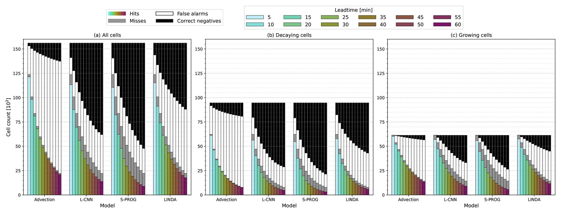
Figure 7 Number of convective cells used in the analysis by nowcast lead time for (a) all cells, (b) decaying cells, and (c) growing cells. Only the cells that are part of the tracks that existed at t₀ are considered. The coloured bars indicate the number of hits, i.e. cells that exist in both target observations and nowcast; the grey bars indicate misses, i.e. cells that exist in target observations but not in nowcast; the white bars indicate false alarms, i.e. cells that exist in nowcast but not in target observations; and the black bars indicate correct negatives, i.e. the number of cell tracks that existed in the input observations at t₀ and do not exist in target observations or nowcast at the given lead time.

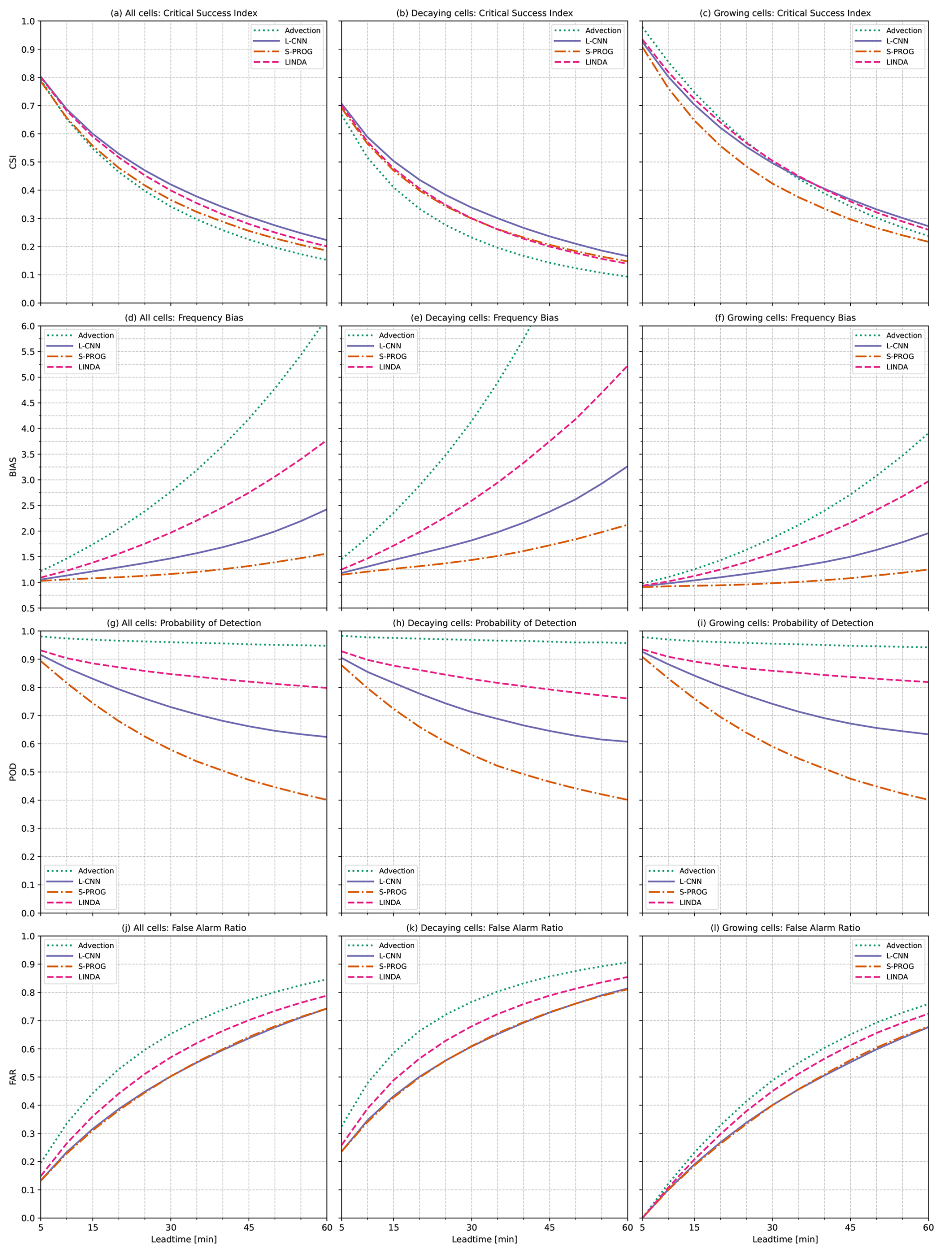
Figure 8 Contingency-based metrics of cell existence as a function of lead time, i.e. whether a cell identified in the target observations was also identified in the nowcast. The panels show the critical success index (CSI) for (a) all cell tracks, (b) decaying cell tracks, and (c) growing cell tracks; the frequency bias (BIAS) for (d) all cell tracks, (e) decaying cell tracks, and (f) growing cell tracks; the probability of detection (POD) for (g) all cell tracks, (h) decaying cell tracks, and (i) growing cell tracks; and the false alarm ratio (FAR) for (j) all cell tracks, (k) decaying cell tracks, and (l) growing cell tracks.

As Figs. 7 and 8 only contain cell tracks that existed when the nowcast was created, the advection nowcast shows a very high POD (Fig. 8d and e), as can be expected. Although the advection nowcast obtains a high POD for both decaying and growing tracks, the behaviour of CSI values in the two groups is different compared with the other models. For decaying tracks, the advection nowcast obtains the lowest CSI (Fig. 8b), whereas it obtains the highest CSI for the growing tracks (Fig. 8c). Because the advection nowcast does not produce decay in rainfall, it will overestimate the existence of decaying cell tracks; however, for growing cell tracks, this becomes beneficial. Note also that the advection nowcast obtains the worst FAR in all groups (Fig. 8g–i), but the difference from the other models is larger for decaying cell tracks.

S-PROG obtains a lower POD than the other models for these metrics. In CSI, S-PROG performs rather well: similar to LINDA and only slightly worse than L-CNN for decaying cell tracks. However, S-PROG has significantly worse performance for growing tracks. The high number of misses, low POD, and best FAR, with values similar to those of L-CNN, indicate that S-PROG loses the cells fastest among all the models, most likely due to blurring.

L-CNN shows the second-largest loss of cells, indicated by the second-worst POD (Fig. 8d–f), FAR values similar to S-PROG (Fig. 8g–i), and a high number of misses (Fig. 7). Compared with S-PROG, L-CNN has more false alarms, indicating that the cell tracks do not die as much as in S-PROG, and more hits, leading to higher CSI for both decaying and growing tracks. L-CNN also has the best CSI for all tracks (Fig. 8a), indicating the best overall skill with respect to reproducing the cell track existence, even though the difference from LINDA is small.

For growing tracks, LINDA has a slightly higher CSI than L-CNN at lead times shorter than 30 min and a slightly lower CSI afterwards. LINDA also has the highest POD after the advection nowcast for both decaying and growing cell tracks. This indicates that LINDA is the best model with respect to reproducing the existence of growing cells and that it produces less decay than the other models, at the expense of a high number of false alarms and an increased FAR (Fig. 8i). For decaying tracks, LINDA has a lower CSI and higher BIAS and FAR than L-CNN, indicating a worse skill in reproducing decay.

Compared to the CSI calculated in a pixel-by-pixel manner (Fig. 5a), the CSI values presented in Fig. 8a–c show different relative behaviour between the models. The pixel-by-pixel CSI measures the skill in predicting exceedance of rainfall at the 4.6 mm h⁻¹ (35 dBZ) threshold and thus penalises, for example, location error and error in the predicted rainfall values. However, the CSI of cell track existence measures only how accurately the existence of the cell track is predicted at each lead time, without considering the area or rainfall distribution inside the cells. While in the pixel-by-pixel CSI (Fig. 5a), L-CNN, LINDA, and S-PROG perform similarly, in the cell track CSI, we see more differences between the models, as described above, especially when differentiating between decaying and growing cells. As such, the cell track CSI provides more detailed insight into how the models predict convective cells, whereas the pixel-by-pixel CSI describes overall forecast skill.

4.3.2 Classification into growing and decaying tracks

In addition to the models' ability to reproduce the cell existence, we also study the goodness of the classification into decaying or growing cell tracks in the nowcasts. The classification is affected by the cell volume rain rate at the input time steps and the first two lead time steps, so the goodness of this classification indicates how well the models reproduce the initial cell development.

Figure 9 shows the number of hits, misses, false alarms, and correct negatives for the classification (Fig. 9a and b) and classification metric values (Fig. 9c). The ETS and GS metrics indicate the overall goodness of the classification, while the other metrics, calculated separately for growth and decay, show the differences in how well the two stages are predicted at the initial lead time steps. Overall, all models show better values for decay in all separately calculated metrics than for growth. This indicates that all models nowcast the initial decay of convective cells better than initial growth.

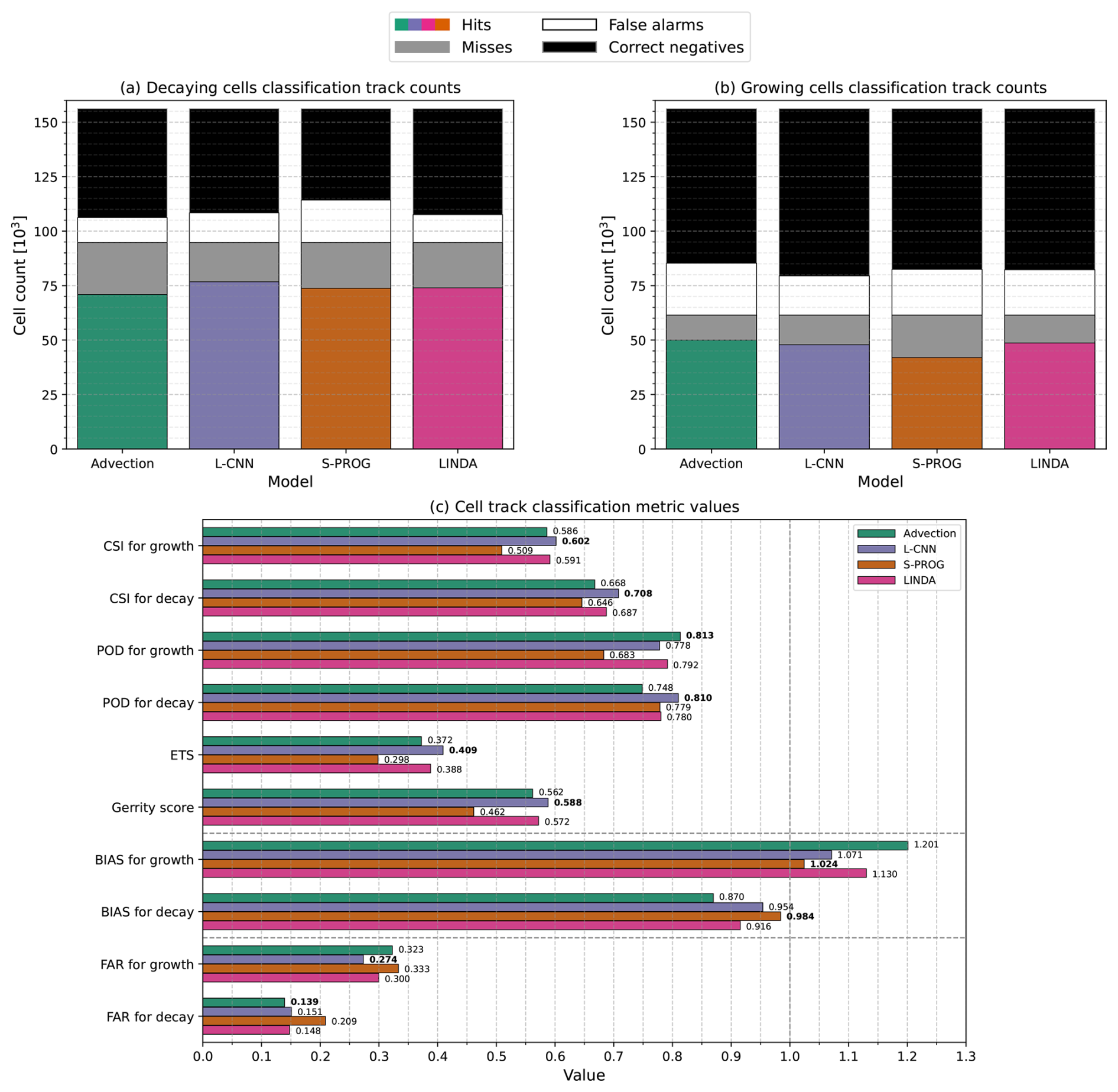
Figure 9 Number of hits (coloured bars), misses (grey bars), false alarms (white bars), and correct negatives (black bars) for the cell track classification into (a) decaying or (b) growing. (c) Contingency-table-based metrics of the track classification into decaying or growing for the models. For the critical success index (CSI), probability of detection (POD), false alarm ratio (FAR), and frequency bias (BIAS), the scores are calculated separately for growing and decaying cell tracks by changing the class that is considered the “true” class. For the equitable threat score (ETS) the score is symmetric, and for the Gerrity score (GS), the multi-category version of the score is used; therefore, only one value is provided for both. The best model for each score is marked in bold. For BIAS and FAR, the value closest to 1 and the lowest value are considered best, respectively, whereas the highest value is the best for other scores.

Overall, based on the ETS and GS scores, the L-CNN model shows the best skill with respect to reproducing the classification and, thus, the initial cell development, with LINDA performing only slightly worse. Comparing the metrics calculated separately for growth and decay, the values are similar, with L-CNN obtaining slightly better values than LINDA for all metrics, except for the CSI for growth and FAR for decay.

The advection nowcast obtains the best POD value for the growing tracks. However, because the cell RVR values do not change significantly in the nowcast in the advection model, the RVR derivative and, subsequently, the classification are controlled largely by the observations at and before t₀, and the high POD is most likely explained by this.

S-PROG performs the worst among the models for all metrics except for the BIAS and POD for the decaying cells. BIAS values close to one indicate a similar number of misses and false alarms but, on their own, do not necessarily indicate actual skill. Even though S-PROG has a higher POD for decaying tracks than the advection nowcast, overall S-PROG shows worse skill in reproducing the initial cell development than the advection, i.e. persistence, nowcast.

4.3.3 Cell features

Figure 10 shows the error distribution of the cell volume rain rate. The errors in the volume rain rate can be roughly decomposed into the errors in the cell area, shown in Fig. 11, and the mean rain rate, shown in Fig. 12. The error distributions are shown separately for all cell tracks and for the decaying and growing cell tracks.

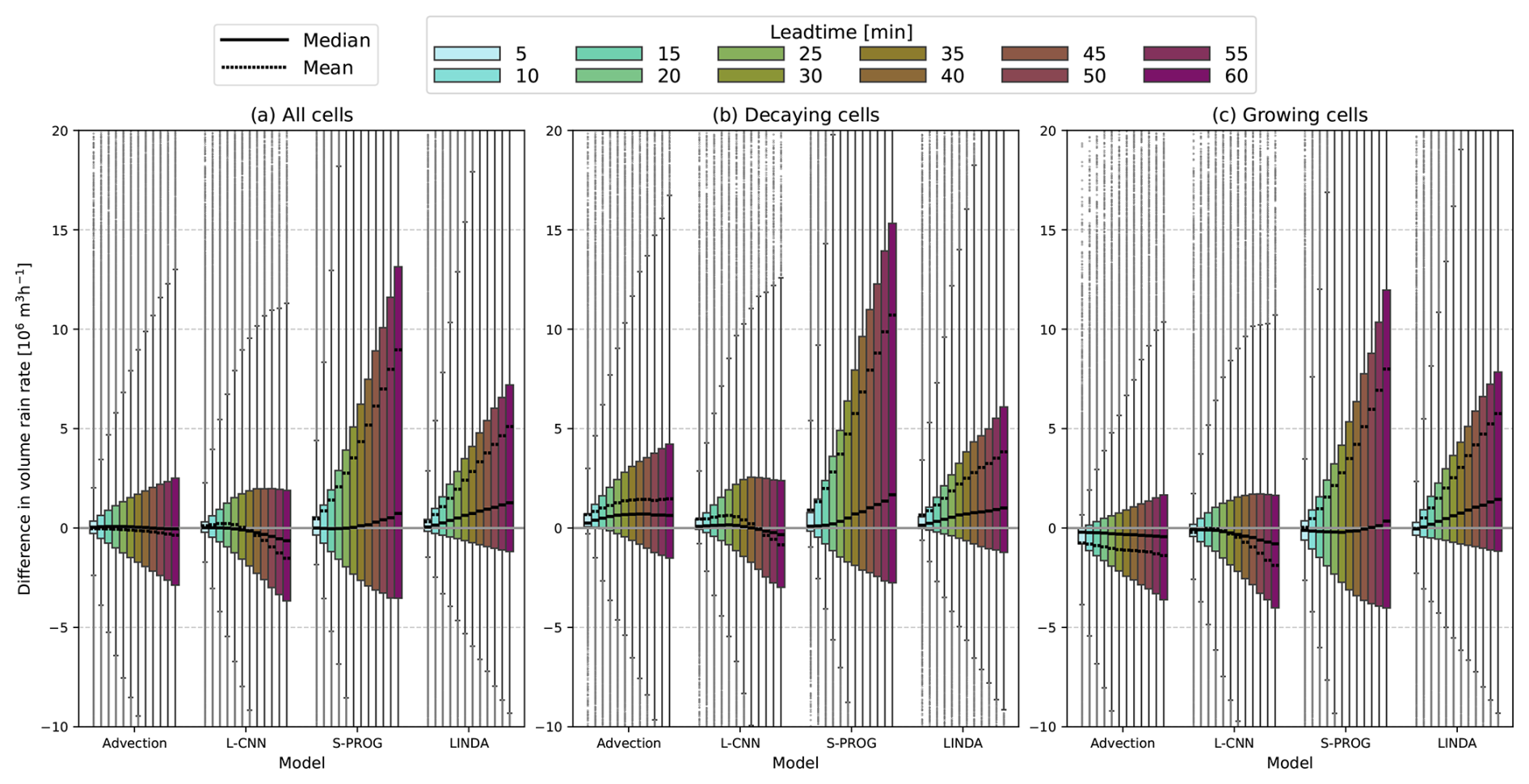
Figure 10 Box plots of differences between predicted and observed cell volume rain rates by nowcast lead time for (a) all cells, (b) decaying cells, and (c) growing cells. The boxes show the 25th to 75th percentile range, while the whiskers represent the 5th to 95th percentile range. The solid line indicates the median, the dotted line is the mean, and outliers are indicated by dots. A positive difference indicates overestimation of the volume rain rate by the model, whereas a negative difference denotes underestimation.

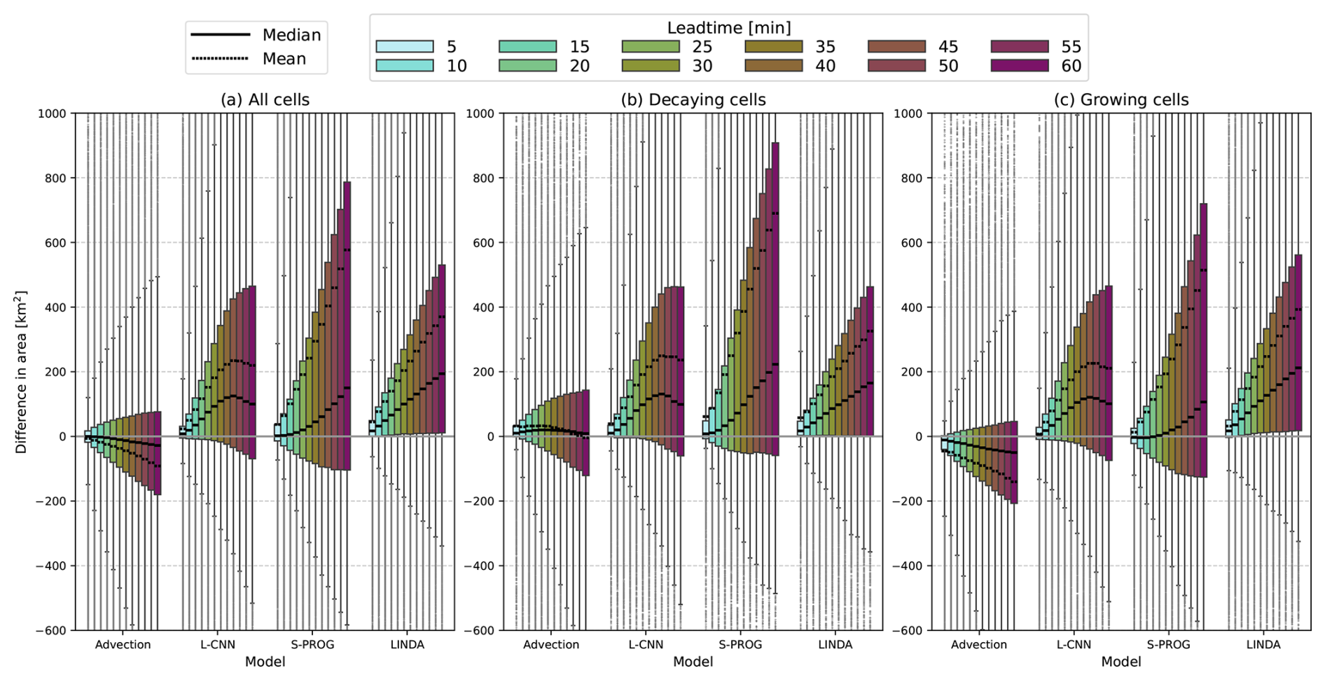
Figure 11 Box plots of differences between predicted and observed cell areas by nowcast lead time for (a) all cells, (b) decaying cells, and (c) growing cells. The boxes show the 25th to 75th percentile range, while the whiskers represent the 5th to 95th percentile range. The solid line indicates the median, the dotted line is the mean, and outliers are indicated by dots. A positive difference indicates overestimation of the cell area by the model, whereas a negative difference denotes underestimation.

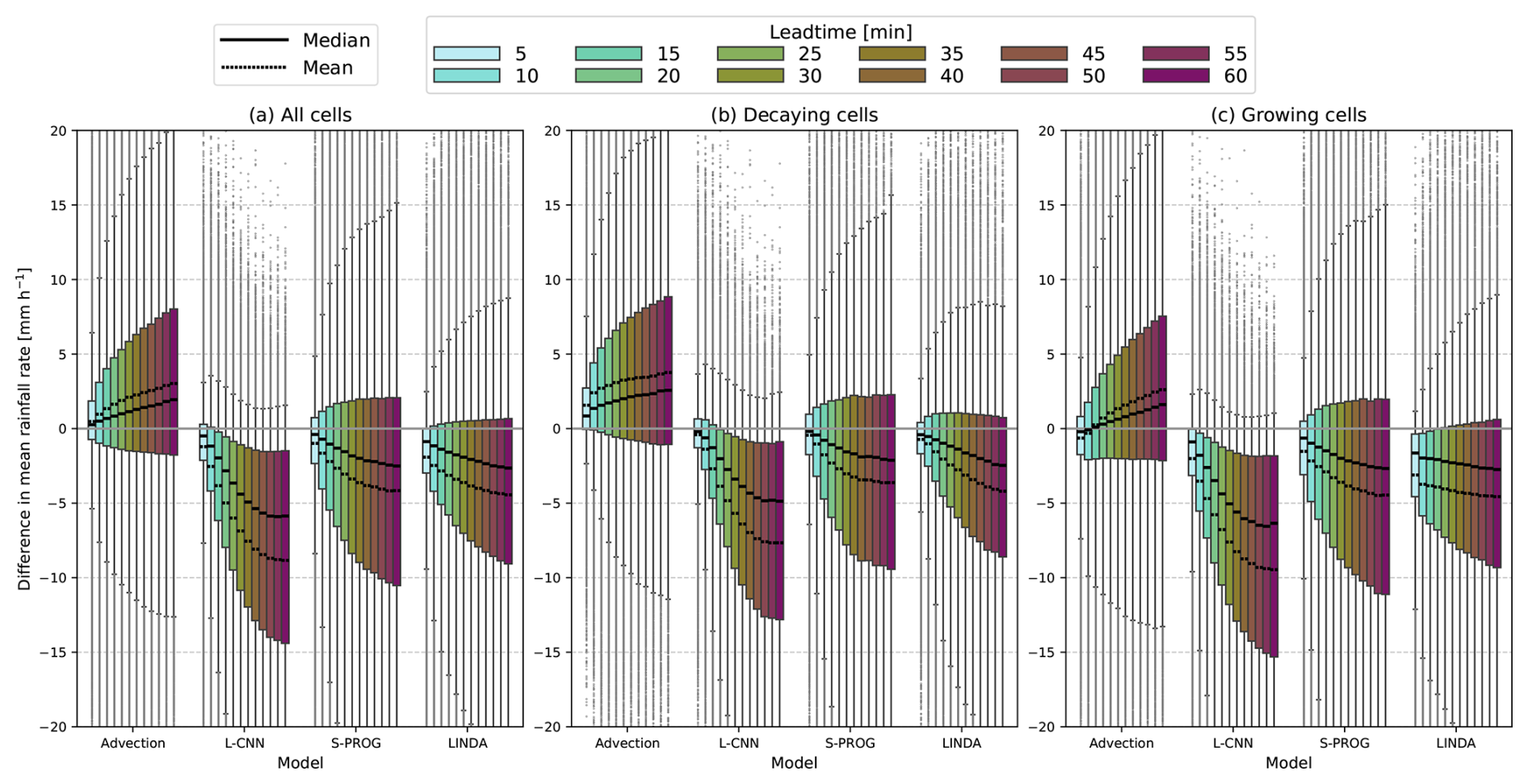
Figure 12 Box plots of differences between predicted and observed mean rain rate inside the cells by nowcast lead time for (a) all cells, (b) decaying cells, and (c) growing cells. The boxes show the 25th to 75th percentile range, while the whiskers represent the 5th to 95th percentile range. The solid line indicates the median, the dotted line is the mean, and outliers are indicated by dots. A positive difference indicates overestimation of the mean rain rate by the model, whereas a negative difference denotes underestimation.

For the advection nowcast, the volume rain rate error distributions for all tracks are highly symmetric, and the median and mean errors are close to zero. However, when decomposed into decaying and growing tracks, the fact that the advection nowcast produces no growth or decay results in an overestimation for decaying tracks and an underestimation for growing tracks. In the cell area error distributions, there is some underestimation of the cell area for all cell tracks as the lead time increases, which largely arises from the growing tracks, as the advection nowcast produces no growth. In the decaying tracks, the advection nowcast has some overestimation of the cell area at short lead times, but the overestimation recedes at lead times longer than 30 min. This could be due to distortions in cell shapes caused by convergence in the motion field. In the mean rain rate, the advection nowcast shows a clear overestimation in both the decaying and growing cell tracks. The tendency for overestimation of the mean rain rate could be caused by (1) a large number of small cells in the dataset where the rain rate decreases as the lead time increases or (2) an irregular rain rate distribution inside cells caused by optical flow interpolation without any smoothing. Nevertheless, the high overestimation of the mean rain rate is compensated for by the underestimation of the area, leading to a narrower error distribution in the volume rain rate.

The L-CNN model has volume rain rate error distributions that are slightly skewed towards underestimation at longer lead times. This is especially visible in the growing cell tracks. The behaviour of the volume rain rate errors is explained by the opposite behaviours of the cell area and mean rain rate error distributions. The L-CNN produces an overestimation in the cell area that increases linearly until 45 min; after this point, the overestimation decreases slightly. However, the mean rain rate shows the opposite behaviour, with an increasing underestimation up to 45 min, after which the mean and median errors plateau. In the mean rain rate, there is little difference between the distributions in the decaying and growing tracks. L-CNN has also smaller median errors in area and volume rain rate than LINDA. This indicates that the localised growth and decay generated by the convolutional neural network in L-CNN can produce more irregular rain rate distributions inside the cells compared with LINDA, which is able to produce only homogeneous development inside the cells due to the Gaussian convolutions in the model. This leads to better estimation of the volume rain rate in L-CNN compared with LINDA.

For S-PROG, the volume rain rate is highly overestimated, mostly because of the large overestimation of the cell areas. This is caused by blurring in the nowcasts, which increases the detected cell size. The wide error distributions are also influenced by the spurious splits and merges that occur in large cells (see Sect. 3.1). In S-PROG, the blurring causes the multiple maxima inside large cells to disappear, leading to more stable cell identification compared with observations that have no blurring, or LINDA and L-CNN, where the blurring is more localised. This leads to an increased number of large errors in the cell area owing to cells that are identified inconsistently in nowcasts and observations. Similar to L-CNN and LINDA, the blurring in S-PROG causes an underestimation of the mean rain rate, although the error distributions also have a larger fraction of values with an overestimation.

Finally, for LINDA, the volume rain rate is largely overestimated, even though the error distributions are less skewed towards overestimation than for S-PROG. For LINDA, the median error in the volume rain rate is always positive also for growing tracks, indicating that LINDA can produce excessive growth in the cells. In the cell area, LINDA shows overestimation, with very similar distributions for both the decaying and growing tracks. LINDA shows the smallest underestimation of mean rain rate. Most likely, the increased growth in LINDA compensates for the blurring, which leads to slightly a more accurate estimation of the mean rain rate.

4.4 Model skill in reproducing cell occurrence

As described in Sect. 3.5, we also study the skill of the models in reproducing convective cell occurrence by identifying the cells at each lead time and matching the cells between target observations and nowcasts. Note that while the metrics presented here are the same as in Sect. 4.3.1, they have different purposes; here, we are investigating how well the models reproduce the overall cell occurrence, without knowledge of the cell tracks. In this definition, the metrics include also skill for the formation of new cells and the decay of all existing cells.

Figure 13a shows the number of cells identified at each lead time from the nowcasts compared with the target observations, separated into hits, misses, and false alarms, and Fig. 13b–e show the metrics calculated from these cell counts. For all models, the number of cells that are matched between the target observations and nowcasts, i.e. hits (coloured bars), decreases as the lead time increases. For S-PROG, the decrease as the lead time increases is steeper than for the other models, which indicates that S-PROG is worse at reproducing the cell occurrence than the other models. This is also supported by the clearly lower BIAS (Fig. 13c), POD (Fig. 13d), and CSI values (Fig. 13b) compared with the other models. On the other hand, S-PROG has the smallest number of false alarms, i.e. cells that are identified in the nowcast but not matched to any cell in target observations, which is also demonstrated by the low FAR (Fig. 13e).

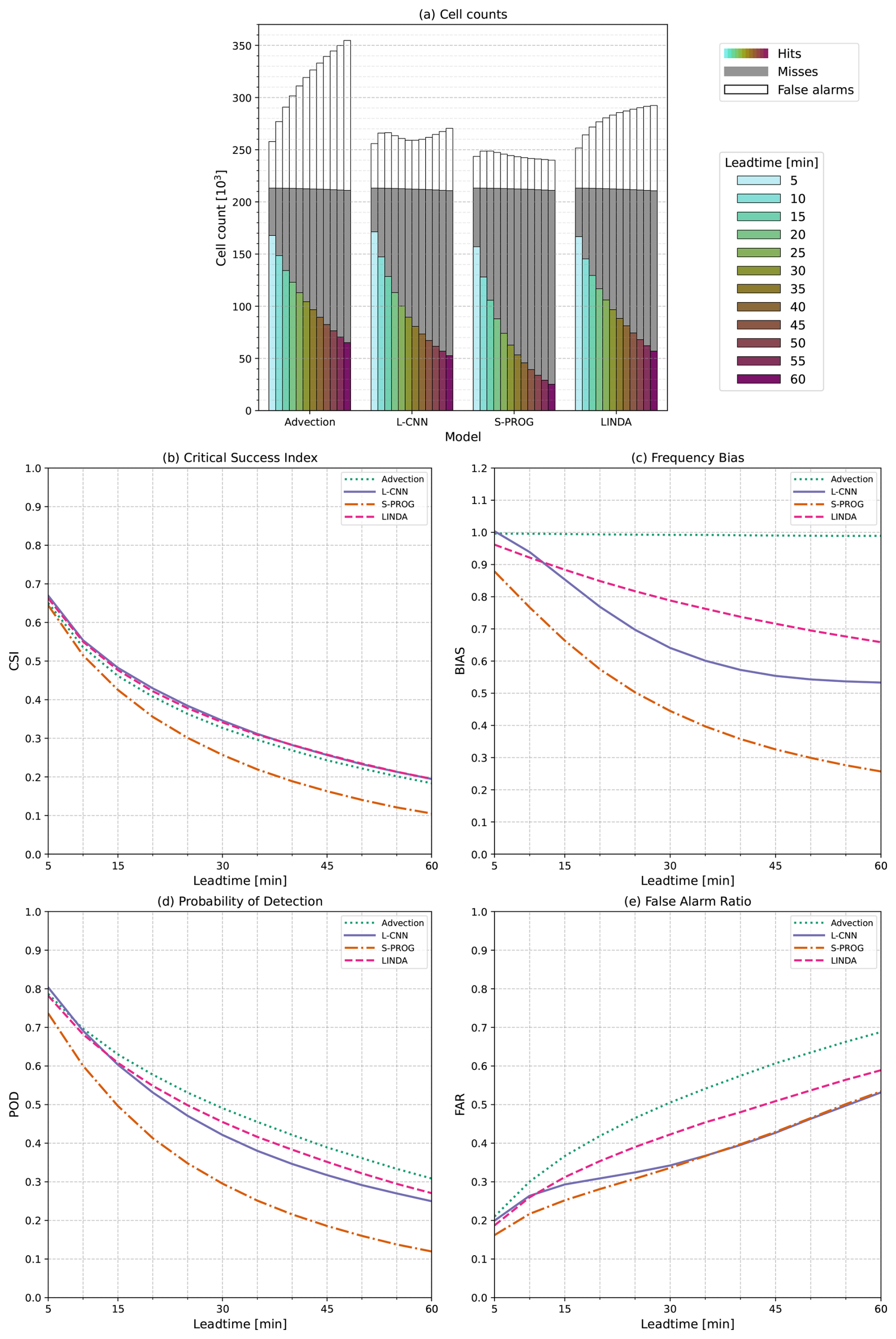
Figure 13 (a) Counts of convective cells by nowcast lead time. (b) Critical success index (CSI), (c) frequency bias (BIAS), (d) probability of detection (POD), and (e) false alarm ratio (FAR) of cell occurrence as a function of lead time, i.e. whether a cell that was identified in target observations was matched to a cell identified in the nowcast. Here, cells are detected and matched in the target observations and nowcasts at each lead time separately, i.e. without considering the cell tracks. In panel (a), the coloured bars indicate the number of hits, i.e. cells that exist in both target observations and nowcast; the grey bars indicate misses, i.e. cells that exist in the target observations but are not matched to any existing cell in the nowcast; and white bars indicate false alarms, i.e. cells that exist in the nowcast but are not matched to any cell in the target observation. Note that, using this definition, the category of “correct negatives” is not defined. The cells are matched with a Hungarian algorithm based on the distance between cell centroids; any matches that are more than 20 km from each other are discarded.

The other models show a very similar distribution of hits and, therefore, a similar CSI. However, the large number of false alarms in the advection nowcast improves the POD and worsens the FAR. Because the number of identified cells changes very little in the advection nowcast, i.e. the numbers of misses and false alarms are similar, the BIAS for the advection nowcast is close to one at all lead times.

Surprisingly, L-CNN does not show a monotonous trend in the number of false alarms, as is seen for the other models; rather, the minimum number of false alarms is seen at a lead time of 30–35 min. This can indicate that the model is generating growth at the later lead times. Compared with LINDA, the decrease in false alarms improves the FAR but lowers the BIAS and POD, whereas the two models perform similarly for the CSI. Notably, L-CNN and LINDA differ very little with respect to the FAR at lead times of 10 min or less. However, for BIAS, L-CNN obtains a value of 1 at the 5 min lead time and decreases quickly after that, whereas LINDA has a lower bias value at the 5 min lead time and a more constant decrease after that. This can indicate that the L-CNN produces little decay at the beginning; however, after the nowcasts begin to decay, it occurs faster than in LINDA, where the decay occurs at a more constant rate.

Comparing the CSI values in Fig. 13b to the CSI values calculated in a pixel-by-pixel manner (Fig. 5a) shows some differences. When the CSI is calculated in a pixel-by-pixel manner (Fig. 5), the advection nowcast has the worst performance and S-PROG performs similarly to L-CNN and LINDA. However, when the CSI is calculated using the identified cells, the advection nowcast shows similar performance to L-CNN and LINDA, whereas S-PROG performs worst. This follows from the different interpretations of the metric. In this cell-based approach, the CSI measures how well the model reproduces the cell existence without considering its exact location (as long as it is close enough to be connected to the cell identified in target observations), shape, or size. From this aspect, the advection nowcast performs well. However, in the pixel-by-pixel framework, CSI describes how well the pixels exceeding the threshold in the nowcast correspond to pixels exceeding the threshold in the observations, and from this aspect, S-PROG performs better due to the blurring increasing the predicted rainfall area.

4.5 Impact of splits and merges in cell tracks

As described previously, the analysis presented in the previous sections used the cell track dataset that included cell tracks with splits and merges. Next, we discuss the impact of splits and merges on the results.

Figure 14 shows (as a function of lead time) the fraction of cells at each lead time that resulted from a cell splitting into multiple cells (split), from multiple cells merging into one (merge), or from both events (see Sect. 3.2). The fractions are shown separately for the target observations and each nowcasting model. In the target observations, at all lead time steps, there is approximately the same fractions of splits, merges, or both. The fractions increase as lead time increases. This is explained by the increasing fraction of long-living cell tracks in the dataset as the lead time increases, as the dataset includes only tracks that existed at t₀. Long-living cell tracks are more likely to consist of large cells and have splits or merges; as their fraction of the dataset increases, the fraction of splits or merges also increases.

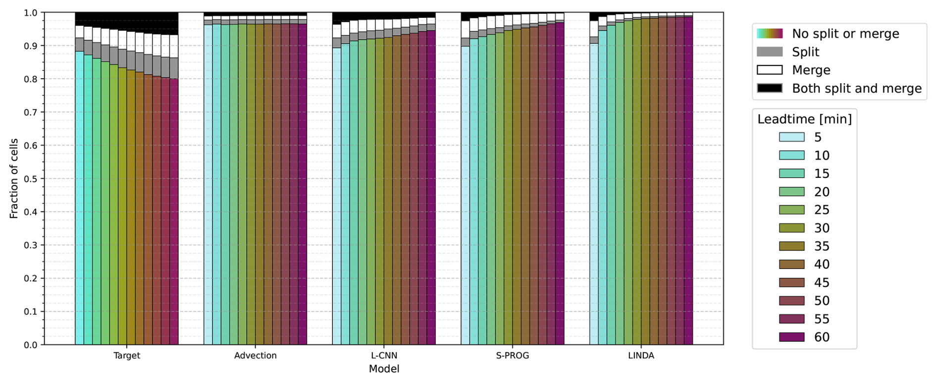
Figure 14 Fractions of splits and merges in the cells as a function of lead time. The coloured bars indicate the fraction of cells that have no splits or merges; grey bars indicate the fraction of cells that are a result of a split; white bars indicate the fraction on cells that have merged from multiple cells; and blacks bars indicate the fraction of cells that result from both a split and a merge. Note that the total number of cells varies for the target observations and each model.

All the nowcasting models clearly reproduce smaller fractions of cells impacted by splits or merges than in the observations, indicating that none of the models could reproduce the splits or merges correctly. The advection nowcast shows approximately constant rates of splits and merges. Because the advection nowcast has no evolution beyond what is caused by convergence or divergence in the motion field, the fraction of splits and merges can be assumed to represent the rate of the spurious splits or merges, i.e. splits and merges caused by the cell identification algorithm that are inconsistent in time (see Sect. 3.1). For the other models, the splits and merges are also caused by the evolution of rainfall fields, mainly blurring in the nowcast fields. Because the impact of the blurring on the smoothness of nowcast fields is larger at the beginning, the models produce more splits and merges at short lead times. The blurring evens the differences between the cells, which results in a larger number of merges than splits. As S-PROG produces the most blurring, it also produces the largest fraction of merges. Notably, compared with S-PROG or LINDA, L-CNN produces approximately the same number of cells impacted by splits, merges, or both, indicating that it reproduces the splits and merges slightly better than the other models.

As described in Sect. 3.2, we provide (in the Supplement) the results repeated for a dataset where the cell tracks containing splits or merges were excluded. Comparing Fig. 4 to Fig. S1 in the Supplement shows that approximately 31 % (for decaying 25 % and for growing 39 %) of cell tracks were excluded. The reason for the larger exclusion rate in the growing tracks is that the majority of the excluded cell tracks have a long lifetime and consist of large cells. From the tracks with RVR$\left(t_{\mathrm{0}}\right)>\mathrm{10}\times {\mathrm{10}}^{\mathrm{6}}$ mm³ h⁻¹, 80 %–90 % were excluded, and from tracks with A(t₀)>400 km², 60 %–100 % were excluded, while from tracks with a smaller volume rain rate or area at t₀, the percentages of excluded cells were smaller. For the maximum area (Fig. 4g–l), the difference between the datasets is similar to that of A(t₀). In the observed track lifetime, the percentage of excluded cells increases from 13 % at a 10 min lifetime to 57 % at lifetimes of 75 min or longer.

This exclusion of long-living tracks with large cells owing to the splits and merges leads to an overall decrease in the skill with respect to predicting the existence of the cells for all models. When comparing the metrics shown in Fig. 8 to those in Fig. S4, clear decreases in CSI values and increases in the BIAS and FAR are visible for all models. For the advection nowcast, L-CNN, and LINDA, the relative skill remains similar; however, for S-PROG, an additional decrease in skill is observed compared with the other models. This is particularly visible in the CSI values for all cell tracks and decaying tracks as well as in the FAR values for all categories. However, for the BIAS values, the other models show higher increases than S-PROG, likely because the large loss of cells due to decay in S-PROG compensates for the increase.

When the cell tracks with splits or merges are excluded, the error distributions of cell feature values (Figs. 10–12 and S6–S8) become narrower and the median and mean errors decrease. This can be attributed to the exclusion of large cells that cause large errors. The narrower distributions are especially visible in the volume rain rate and area; the impact is less visible for the mean rain rate. However, the overall trends in median errors remain similar. Additionally, there are only small differences in the model skill with respect to reproducing the cell track classification at t₀ (Figs. 9 and S5).

Overall, the comparison of the results shows that including tracks with splits and merges improves the model skill in reproducing cell track existence but increases the error in predicted cell features. That is, the models can predict the existence of the most representative cell track but not its feature values for cell tracks with splits or merges.

5 Discussion and conclusions

The aim of this study was to develop a framework to investigate how accurately nowcasting models reproduce the development of convective rainfall. The framework consists of identifying and tracking the convective cells in the observations and nowcasts and comparing different cell features between equivalent cell tracks in observations and nowcasts. This approach allows the study of how well the existence of cells is predicted as well as how accurately the different features of the cells are reproduced by the models. By examining various cell features, such as the cell volume rain rate and area, we can quantify the differences between how the models produce growth and decay in convective rainfall. Furthermore, by tracking cells from the initial observational inputs used in the models, the framework enables an investigation into how the initial state of convective cells impacts nowcast quality. Compared with standard verification methods, the framework enables separate analysis of various aspects of the nowcasting models' skill for convective rainfall, offering more detailed information to support model development.

The framework was demonstrated using four advection-based, openly available models: advection nowcast, S-PROG, LINDA, and L-CNN. The models were compared using data from the Swiss radar network and a dataset that largely consisted of small convective cells. To investigate the impact of the initial conditions, the cell tracks were classified into tracks that were decaying or growing at the time when the nowcast was created. The results indicate that the advection nowcast can predict the volume rain rate of the cells relatively well, even though it does not create growth or decay in the nowcasts. The L-CNN model was found to best reproduce the existence of convective cells, with a small improvement over LINDA. Even though L-CNN had a slightly smaller error in the cell volume rain rate and area than LINDA owing to the more localised decay predicted by the convolutional neural network in L-CNN, LINDA predicted the cell mean rain rate more accurately. The S-PROG model adequately reproduced the existence of decaying cells, but it also produced the largest overestimations of cell area and volume rain rate.

The proposed framework allowed us to quantify several qualities in the models, such as differences in how L-CNN, LINDA, and S-PROG produce smoothing, which are not easily distinguishable in the pixel-by-pixel verification metrics usually used for nowcasting model validation. Quantifying these aspects of the models aids in model development and in selecting the most suitable nowcasting model for each application. For example, for an application where predicting the volume rain rate correctly is important, such as predicting rainfall accumulation, the L-CNN might be the best among the four models. However, if the correct areal extent of convective rainfall is important, advection nowcast will perform better. Because the models are studied using only the cells identified in the observations and nowcasts, the cell identification and tracking algorithms can be adjusted to specifically describe the convective cells that are significant to the application in question.

However, compared with pixel-by-pixel verification, this framework has certain limitations. Because the dataset is composed of the identified convective cells, the results are sensitive to the selected cell identification and tracking methods as well as to how, for example, splits and merges are processed. Furthermore, the impact of the identification and tracking algorithms can vary between the models, for example, if the blurring in the models is different and impacts the cell identification. Additionally, interpreting the results requires expertise in the models studied and knowledge of the underlying dataset, which might make the framework less suitable for use by inexperienced end-users. The complexity of the framework and the sensitivity to selected cell identification and tracking algorithms also make possible comparison between different studies difficult. However, the variety of the results and the possibility of adjusting the framework provide extensive tools for model developers.

The sensitivity to the selected cell identification and tracking methods and their parameters is also the largest source of uncertainty in the results. Because the methods used here are deterministic, we do not obtain estimates of the uncertainty in identified cells or their tracks. This could be addressed in future research, for example, by estimating the sensitivity of the cells to the identification threshold or other parameters set in the methods. Other sources of uncertainty include the splits and merges occurring in the cell tracks, which can be addressed by estimating the impact of the cell tracks with splits or merges to the results, as was done in this study. Further uncertainty in the framework is caused by uncertainty and errors in the weather radar observations that can impact the results, for example, through errors in cell identification. This should be addressed foremost through data quality control, as such artefacts in the observations would most likely also reduce the nowcast quality.

Because the results are sensitive to the identified cells, adjusting the cell identification and tracking algorithms also provides opportunities for more complex analysis of the models or weather phenomena. These analyses would be especially interesting for models that are able to produce non-smoothed nowcasts, such as generative ML models. For example, the models' ability to reproduce the splitting and merging in the cell tracks could be evaluated by applying a cell-tracking algorithm that processes the splits and merges using a more sophisticated procedure (e.g. Limpert et al., 2015; Zan et al., 2019). On the other hand, applying a cell detection algorithm capable of identifying cells hierarchically (e.g. Hou and Wang, 2017) would allow for the evaluation of how accurately the models reproduce complex weather phenomena, such as longer-living, multi-cell convective systems.

The presented framework also allows for the study of the impact of the initial conditions of the convective cell on how well its development is predicted. In addition to the initial stage of the cells, which were divided into decaying and growing stages here, another interesting application of the framework would be to study the impact of additional input data sources on the forecast skill. Several studies have shown that additional input data sources, such as numerical weather prediction model data or polarimetric radar measurements, can improve the performance of ML nowcasting models (Sønderby et al., 2020; Pan et al., 2021; Zhu et al., 2022; Lu et al., 2023). The presented framework can be utilised to quantify the impact of data sources on the forecast convective cell development by differentiating the cell tracks based on the data observed in the cells in the input time steps.

The proposed framework is analogous to tropical cyclone tracking used as a verification method, for example, for global ML weather forecasting models (Bi et al., 2023; Newman et al., 2023), applied to high-resolution rainfall forecasts in smaller domains. Although we presented the framework using deterministic models, it can be applied similarly to probabilistic models by applying the cell identification and tracking to each ensemble member separately. In probabilistic models, the ensemble members should be diverse to better capture a wide range of events, and, for example, predicting the correct location of rainfall is not as important as for deterministic forecasts. Because the presented framework considers several aspects of convective cell evolution and is not dependent on the correct location, it can be used to study how well cell evolution is reproduced in ensemble members.

Other possible future developments and applications of the proposed framework would be to extend the cell tracking to cover the entire life cycle of the convective cells, not only the first hour, as was done here. This would be especially interesting when investigating generative ML models that can create nowcasts without blurring for long lead times (Ravuri et al., 2021; Zhang et al., 2023). Because the nowcasts do not have blurring and, therefore, appear realistic to the user, the framework could be used to quantify how realistically the models reproduce convective cell development and, thus, contribute to a greater understanding of the usefulness of such methods when predicting extreme high-intensity rainfall.