Quantifying the analysis uncertainty for nowcasting application

This study proposes a method to quantify uncertainty represented by errors in very-high-resolution near-surface analysis, specifically for weather nowcasting applications. Gaussian distributed perturbations are used to perturb the first guess and observation with a variance equal to that of the first-guess error. This error reflects the spatial characteristics of the difference between the first guess and observations and dominates the primary sources of analysis uncertainty. However, mapping perturbations to analyse the grid mesh through interpolation results in underdispersion, particularly in areas without stations. To address this issue, Gaussian perturbations are inflated with an inflation factor to amplify the dispersion. This method was applied to high-resolution analysis and nowcasting for hourly temperature, humidity, and wind components in the Beijing–Tianjin–Hebei region to assess its effectiveness in representing uncertainty. The generated ensemble analysis exhibits reasonable spread and high reliability, indicating accurate quantification of analysis uncertainty. Ensemble nowcasting is extrapolated from ensemble analysis to evaluate the transmission of perturbation during extrapolation. Verification results of ensemble nowcasting reflect the fact that the spread increases effectively during extrapolation up to a lead time of 6 h. However, the increase in the spread is highly dependent on the persistence of numerical weather prediction. The results demonstrate that generating appropriate perturbations based on analysis errors effectively represents the analysis uncertainty and contributes to estimating uncertainty in nowcasting.

1 Introduction

Nowcasting is crucial for severe weather warnings and for protecting life and property, as it rapidly predicts high-impact weather events in near real time (Wang et al., 2017a, b; Wastl et al., 2018; Schmid et al., 2019). A very-high-resolution weather analysis forms the basis for skilful nowcasting, providing accurate real-time atmospheric conditions at the initial time (Wastl et al., 2021). However, due to the chaotic nature of the atmosphere, errors in the data, and imperfect numerical models, nowcasting involves uncertainties (Lorenz, 1965; Leith, 1974; Kann et al., 2012; Glahn and Im, 2013; Wastl et al., 2019). To deal with uncertainties, generating an ensemble using appropriate perturbations is an effective approach (Leutbecher et al., 2007; Leutbecher and Palmer, 2008).

In recent years, the use of ensemble nowcasting has become increasingly widespread (Wang et al., 2017b, 2021; Yang et al., 2023). Numerous studies have demonstrated that addressing all sources of the uncertainty represented by errors is a key aspect of generating ensembles (Sun et al., 2014; Thiruvengadam et al., 2020). The weather analysis contains uncertainty, which significantly impacts nowcasting due to both measurement errors and computational errors (Eibl and Steinacker, 2017; Keresturi et al., 2019). As a result, quantifying uncertainty caused by these errors in analysis is one of the major challenges in constructing ensemble nowcasting (Wang et al., 2017a; Taylor et al., 2022).

A widely applied approach for quantifying uncertainty is introducing appropriate perturbations to generate ensembles, based on the characteristics of errors (Buizza et al., 2005; Zhu, 2005; Bouttier et al., 2016; Chen et al., 2016; Wang et al., 2017a; Lin et al., 2022). Most studies focus on addressing uncertainty in nowcasting, but few have explored the impact of analysis errors (Bouttier, 2019; Wang et al., 2021). Wang et al. (2014) and Suklitsch et al. (2015) presented evidence that introducing additional perturbations to estimate the analysis uncertainty can improve the simulation of nowcasting uncertainty. Saetra et al. (2004) explored the influence of observation errors on analysis uncertainty. Horányi et al. (2011) and Bellus et al. (2016, 2019) demonstrated that appropriate perturbations can simulate observation uncertainty in analysis. The Aire Limitée Adaptation dynamique Développement InterNational-Limited Area Ensemble Forecasting (ALADIN-LAEF) and Convection-permitting Limited-Area Ensemble Forecasting (C-LAEF) systems are two skilful systems that use 16 members to represent analysis uncertainty. These systems account for uncertainty by perturbing observations, while the 16 first guesses provide important uncertainty information within the three-dimensional background (more details can be found in Wang et al., 2011, Bellus et al., 2016, and Wastl et al., 2021). However, neither ALADIN-LAEF nor C-LAEF addresses the impact of other sources of uncertainty, such as those arising from interpolation (Wastl et al., 2021). Therefore, considering various types of analysis errors is crucial for more accurately quantifying analysis uncertainty (Suklitsch et al., 2015).

An accurate analysis, which describes the current atmosphere, is typically derived by assimilating the first-guess and observation data (Randriamampianina and Storto, 2008; Kann et al., 2009; Lin et al., 2022). Observations estimate true atmospheric values, while the three-dimensional first guess offers a comprehensive spatial structure for the region of interest (Sun et al., 2013; Hoteit et al., 2015; Casellas et al., 2021). However, when combining observations with terrain-corrected first guesses, interpolation errors caused by the algorithm may also arise (Leutbecher and Palmer, 2008; Feng et al., 2020). Current research has not clearly addressed the impact of interpolation error uncertainty on the analysis and nowcasting. Hence, it is crucial to investigate how to accurately estimate interpolation error in analysis in order to gain a comprehensive understanding of both analysis and nowcasting uncertainty.

The Integrated Nowcasting through Comprehensive Analysis (INCA) system calibrates the first guess using automatic weather station observations (Haiden et al., 2010, 2011). The first guess in INCA is the numerical weather prediction (NWP) field, which is provided by the Austrian operational version of the ALADIN limited-area model, as described by Wang et al. (2006). In the NWP calibration, a topographic characteristic factor is used to correct the surface layer to match the actual terrain (Kann et al., 2009). Seamless Integrated Weather Prediction and Applications (SIVA) is a multivariable analysis and nowcasting system based on the INCA framework, and it is applied in the Beijing–Tianjin–Hebei (BTH) region in China. The NWP output of the China Meteorological Administration Mesoscale model (CMA-MESO) provides a deterministic first guess, which is used by SIVA to describe the spatial characteristics (Shen et al., 2020). Since the first guess is deterministic, the uncertainty of SIVA analysis is not considered. Therefore, it is necessary to consider the computational errors to accurately quantify the uncertainty in SIVA analysis.

The current methods for estimating uncertainty in analysis primarily depend on perturbations either derived from the first guess or generated based on the inherent errors in observation data (Horányi et al., 2011; Wang et al., 2017a; Wastl et al., 2018; Yang et al., 2023). These approaches introduce perturbations without accounting for the uncertainty intrinsic to the analysis calculation process. Nevertheless, they provide valuable insights, suggesting that perturbations can be generated according to the statistical characteristics of errors. Building upon this foundation, this study proposes a novel approach that generates perturbations based on errors in the calculation process itself, offering a more comprehensive way of quantifying analysis uncertainty. This approach addresses the limitations of current techniques and enhances the precision of uncertainty representation. It has significant potential to improve ensemble nowcasting applications.

This article is organized as follows. Section 2 introduces the algorithm of SIVA analysis. Section 3 elaborates on the characteristics of errors and perturbation methods. Section 4 is dedicated to the verification results of ensemble analysis and nowcasting. A summary and conclusions are given in Sect. 5.

2 Method and data

SIVA provides hourly analysis and nowcasting fields at a horizontal resolution of 1 km for near-surface temperature, humidity, and wind speed components. The analysis starts with a first guess, which is a NWP short-range forecast output of CMA-MESO. CMA-MESO runs twice daily with a forecast range of 48 h, starting at 00:00 and 12:00 (UTC). It has a horizontal resolution of 3 km and 51 vertical levels. The forecast field of CMA-MESO is interpolated to a SIVA grid mesh at a horizontal resolution of 1 km to serve as the first guess, which is then calibrated based on its errors relative to observations. Topographic parameters are used to map the heights of CMA-MESO model levels to the actual altitude of the station location. The observations used in this research, considered the ground truth, are provided by automatic weather stations and include hourly 2 m surface temperature, specific humidity, and 10 m surface wind speed. These data can be obtained by submitting an application through the official data platform of the China Meteorological Administration. The algorithm for the 2 m temperature, humidity, and 10 m wind speed analysis module of SIVA consists of the following steps:

• Step 1. Revise the first guess by inverse distance weight interpolation (IDW) using ground observation data to obtain a three-dimensional revised field (3DRF). The interpolation process in this step is referred to as 3D interpolation.

• Step 2. Combining the topographic features and observation data, the 3DRF is revised again and then interpolated vertically to the lowest model level to obtain the near-surface revised field (NRF). The interpolation process in this step is denoted as 2D interpolation.

Since SIVA is a new version of INCA developed in the BTH region, readers can find more details of the algorithm in Haiden et al. (2010, 2011). To avoid confusion of the term “error”, the difference between the first guess and observation in Step 1 is denoted as “error1”. The difference between the 3DRF and the observation in Step 2 is denoted as “error2”. The experimental periods are August 2020 (hereafter called summer) and February 2021 (hereafter called winter). With the high horizontal resolution, SIVA can describe the geographical features in detail. In addition, 21 vertical levels corresponding to various altitudes, such as 0, 200 m, and up to 4000 m above the ground, are used to match stations at different elevations. The wind speed is represented at 32 vertical levels with intervals of 125 m. This approach ensures that the first guess is calibrated using topographic parameters and observations at the station locations. This study discusses three meteorological elements: temperature (T_2 m), humidity (relative humidity RH2m and specific humidity QQ_2 m) at 2 m above the surface, and wind speed components (U_10 m and V_10 m) at 10 m above the ground.

BTH has a unique and complex topographic structure, with the north-western part between two mountain ranges and the south-eastern part belonging to the North China Plain (Fig. 1). Such topographic information and station altitude are used to impose terrain constraints on the SIVA grid points. The 1670 automatic weather stations can pass quality control and are used for T_2 m and humidity analysis. For wind components, 2351 stations are available. To assess the effectiveness of ensemble analysis in representing uncertainty, 151 stations are randomly selected as the test set, while the remaining 1519 stations are the training set and then are used to generate the ensemble analysis and nowcasting (Fig. 1). Since the wind components have different quality control frameworks with temperature, the total number of stations for wind is 2350, while the number of test stations is 191.

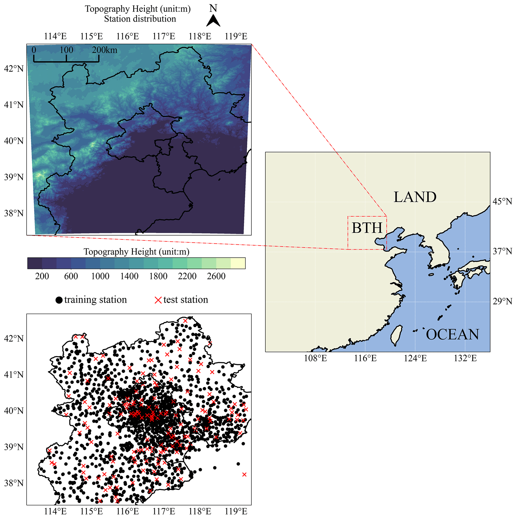
Figure 1 Topography height (m) and station distribution over the Beijing–Tianjin–Hebei (BTH) region. Black dots represent training stations and red dots represent test stations, both used for T_2 m and QQ_2 m.

This work proposes a perturbation method to accurately quantify the uncertainty represented by the errors in the analysis. These errors depend on the observations, which can only be obtained in areas with station information and interpolated across the entire grid mesh. Therefore, the magnitude of the perturbation is expected to be consistent with the statistical characteristics of these errors, as observed at the training stations (Fig. S1 in the Supplement). In addition, the test stations assess whether interpolation can effectively propagate the perturbation information throughout the entire space. To evaluate the impact of the perturbation on extrapolation, the perturbed analysis is used to generate ensemble nowcasting. The ensemble nowcasting starts hourly and extrapolates up to a lead time of 6 h. The verification of both ensemble analysis and nowcasting covers the test stations shown in Fig. 1.

3 Perturbation method

For T_2 m, error1 is based on the principle of minimal required correction to filter out the excessive forecast errors, which may result in some instances where the error value is zero, even though the true error1 value is non-zero. Therefore, the forecast error of NWP causes a major source of uncertainty in error1. Due to the terrain constraint, the spatial distribution of error1 and error2 exhibits distinct topographic features, and the analysis error will reflect these geographic characteristics (Fig. S1). As described by Horányi et al. (2011), perturbations are generated by the standard deviation (SD) of the errors to represent the uncertainty at the observation site. Hence, the observation perturbation in this study is generated based on the SD of error1 at the training station sites. Error1 is the difference between the first guess and observation and is represented at the training station locations. This means that at each training station the observation perturbation is sampled randomly from Gaussian noise with a mean of 0 and a scale equal to the SD of error1. However, both error1 and the observation perturbation are extrapolated to the entire grid mesh through interpolation, which means that the areas without stations (hereafter called the area with test stations) can only have partial information on error1 and the perturbation. Therefore, to account more comprehensively for uncertainty across the entire grid mesh, the perturbation of the first guess is crucial, as the first guess is responsible for providing a calibrated forecast in areas without observations.

To estimate the uncertainty across the entire space, the SD of error1 is interpolated to the SIVA grid mesh to perturb the first guess. At each grid point, the perturbation (hereafter called first-guess perturbation) is a Gaussian noise with a mean of 0 and an SD equal to that of the interpolated error1. Since error1 is the distance between the first guess and the observation at the lowest model level, it implies a downward (upward) shift that aligns the model height with the true altitude of the station location. This indicates that in vertical interpolation the forecast error will combine with geographical features. In addition, interpolating the 3DRF to the surface level depends on the vertical errors between adjacent levels. Hence, the first-guess perturbation is sampled from Gaussian noise with a shape (M,Z), where M represents the number of members and Z denotes the number of levels. Such first-guess perturbation can represent the NWP systemic uncertainty in the vertical dimension, while the horizontal distribution of the interpolated error1 provides the spatial characteristic.

As described above, both the observation perturbation and the first-guess perturbation are generated based on the errors in analysis and within areas that have observation information. Introducing these perturbations into the observation and first guess, ensemble analysis is constructed. To evaluate the representation of the uncertainty, the ensemble is interpolated to all the stations and uses the observation data to verify its reliability. Figure 2 shows the root-mean-square error (RMSE) and ensemble spread at both the training and test stations. The spread quantifies the dispersion or variability among the ensemble members, while the RMSE represents the errors of the ensemble mean. Comparing the spread and RMSE assesses the statistical reliability of the ensemble. A reliable ensemble should exhibit alignment between the spread and the RMSE (Fortin et al., 2014). It can be observed that the spread in training stations is consistent with the RMSE (Fig. 2a, b). The ratio of RMSE to spread is nearly equal to 1 (Fig. 2c). This indicates that the uncertainty in area with station information has been quantified appropriately. There is a significant underdispersion at the test stations (Fig. 2d, e). This underdispersion can be interpreted as the information in the area without the stations being sufficient. However, in the concept of appropriate representation of uncertainty, the spread in the test stations should be amplified to be equal to the RMSE.

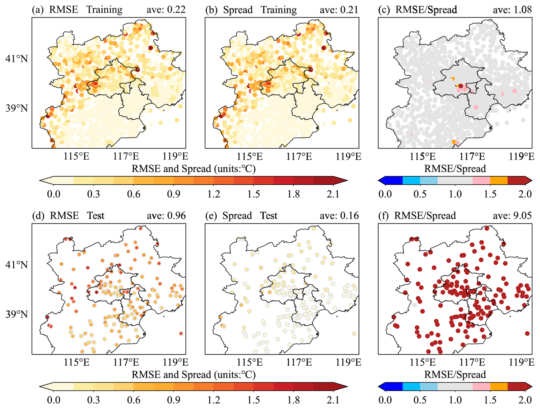
Figure 2 RMSE of the ensemble mean (a, d), spread of the ensemble (b, e), and the ratio of the RMSE to the spread (c, f) for T_2 m at both the training and test stations. All the values are averaged over August 2020.

An inflation factor is calculated to address the underdispersion at the test stations. The inflation factor is the ratio of the RMSE to the spread (R_rs) at the test stations in the ensemble analysis obtained by perturbing both the first guess and the observation (e.g. as shown in Fig. 2f). This factor is then interpolated to the grid mesh to amplify the SD of the first-guess perturbation in the area with the test stations, thereby ensuring that the spread aligns with the RMSE (Fig. S2).

By combining an inflation factor with the perturbations, these are generated as follows:

$$\begin{array}{}\text{(1)}& {\displaystyle }\begin{array}{rl}{\mathrm{NWP}}_{(i,j)}^{\prime }& ={\mathrm{NWP}}_{(i,j)}+N(\mathrm{0},{\mathrm{SD}}_{\text{2D error1 (i,j)}}\\ & \cdot \mathrm{infla}\mathrm{\_}{\mathrm{factor}}_{(i,j)}),\end{array}\text{(2)}& {\displaystyle }{\mathrm{OBS}}_k^{\prime }={\mathrm{OBS}}_k+\mathrm{N}(\mathrm{0},{\mathrm{SD}}_{\mathrm{error}\mathrm{1}\left(k\right)}).\end{array}$$

Here, 2D error1 represents the interpolated SD of error1. The subscripts (i,j) and k refer to the SIVA grid point and the kth station, respectively. It should be emphasized that the observation of wind has not been perturbed. The true values of the wind components are obtained through the sine and cosine transformations. Therefore, perturbing the wind components through error-based noise cannot reflect the uncertainty arising from the wind direction.

The principle of minimal required correction in T_2 m analysis results in a significant reduction in the dispersion of the perturbed error1 relative to the unperturbed error1. Nevertheless, the impact of the inflation factor guarantees that the dispersion of ensemble errors will not attenuate excessively (Fig. 3a, b). The error dispersion at both the training and test stations aligns with the perturbed error1. This consistency substantiates the reliability of this approach, involving the introduction of the inflation factor in representing uncertainties. The generated ensembles consistently represent uncertainty with comparable reliability across the entire region (Fig. 3). Furthermore, the results of ensembles with varying members differ by only about 1 %. To balance computational efficiency with the need for sufficient members, the ensemble size is set to 20.

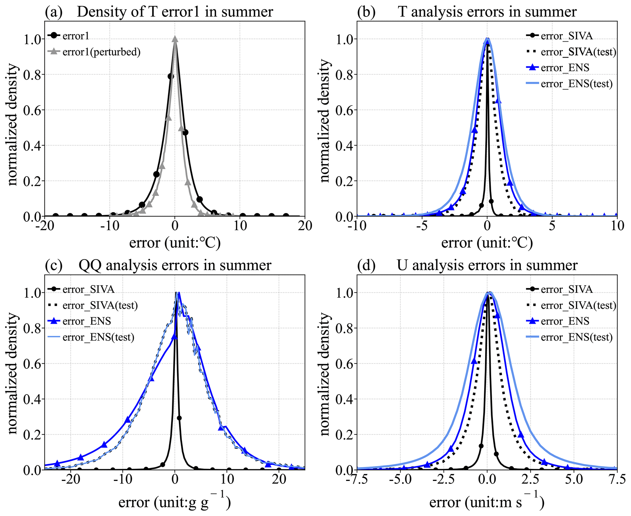
Figure 3 Probability density function (PDF) of errors. Panel (a) shows error1, where the thick black line (•) represents the unperturbed error1 and the thin grey line (▴) represents the perturbed error1. Panels (b–d) show the analysis errors of the temperature, specific humidity, and U component of the wind speed. The black solid and dashed lines represent the PDFs of SIVA deterministic analysis errors at both the training and test stations, respectively. The blue and light-blue lines represent the PDFs of the ensemble analysis errors at the same stations.

4 Verification

4.1 Verification of the ensemble analysis

The deterministic SIVA analysis (hereafter called CANA) served as a reference for assessing the performance of the generated ensemble in estimating uncertainty at test stations. Commonly used probability verification scores, including the RMSE, ensemble spread, Talagrand diagram, rank histogram, and reliability diagram, are applied to evaluate the effectiveness of the uncertainty representation at the test stations (Hamill et al., 2000; Hamill 2001; Fortin et al., 2014).

4.1.1 Ensemble RMSE and spread

For the verification of the T_2 m, QQ_2 m, and RH2m ensembles, a total of 151 stations is used. One station in the south-east is only available in summer, and there are 150 test stations in winter. There are 191 test stations to evaluate the performance of wind components. Table 1 presents the averaged RMSE and ensemble spread for the meteorological elements discussed in this research.

Table 1 RMSE and spread of the ensemble analyses for summer (August 2020) and winter (February 2021). The subscript C (E) denotes the RMSE of CANA (ensemble analysis), and R_rs represents the ratio of the ensemble RMSE to the spread. Values are averaged over all the test stations and the entire period.

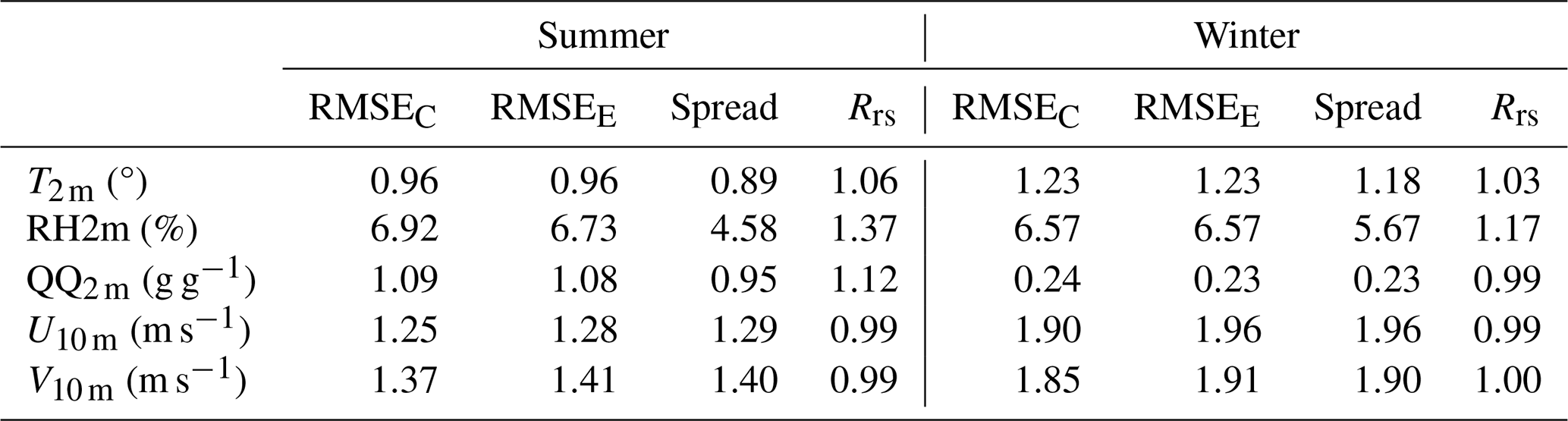
Without inflation, the averaged ensemble spread is around 0.16, while the RMSE is approximately 10 times larger (Fig. 2d–f). This reflects the considerable underdispersion of the ensemble (Fig. 4a, d). By introducing the inflation factor, the ensemble spread increases to 0.89 and R_rs approaches 1, indicating that the ensemble exhibits reliable dispersion. Moreover, the increase in the spread of both temperature and humidity does not result in a corresponding increase in the RMSE (Table 1). This is attributed to the zero mean of the perturbations, allowing the inflation factor to adjust only the SD without affecting the mean.

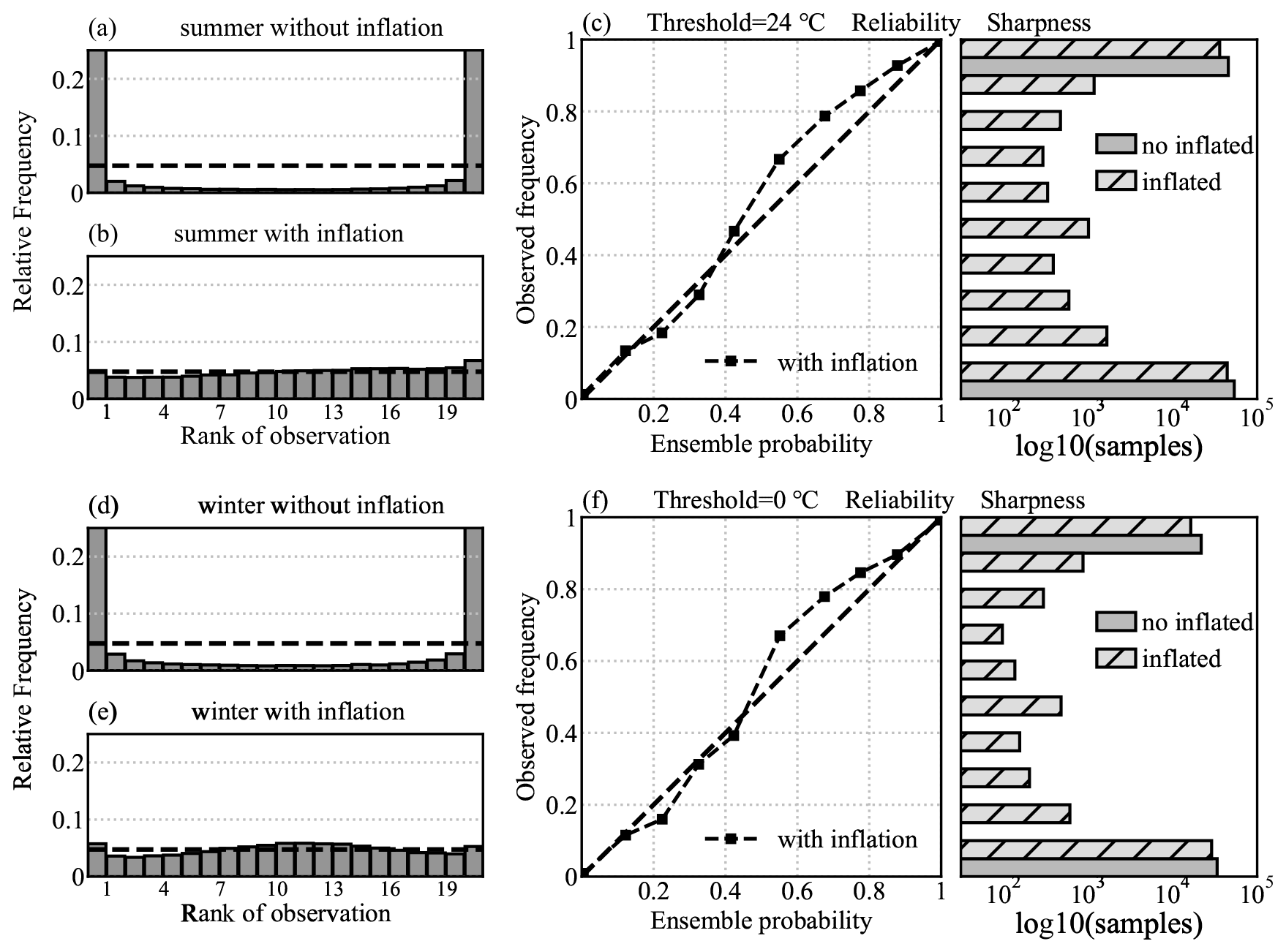
Figure 4 Talagrand (a, b, d, e) and reliability (c, f) diagrams for T_2 m ensemble analysis, averaged over all the test stations.

This work focuses primarily on quantifying analysis uncertainty rather than achieving dramatic improvements in verification scores. With the effect of the inflation factor, the perturbation in the corresponding grids of the test stations is amplified to align the ensemble spread with the RMSE. In addition, the perturbed first guess reflects the spatial uncertainty at the grid points. Hence, the distance weight in the 3D interpolation of the 3DRF can account for the uncertainty derived from the geographic characteristics of CMA-MESO. Most test stations have a spread nearly equal to the RMSE, indicating the accuracy of the uncertainty quantification (Fig. S3). In mountainous areas, the RMSE is negatively affected due to the lack of precise information on the inversion heights (Fig. S3g). A marine station in the south-east receives perturbation information mainly from the 3DRF and only a small amount of NRF information during the summer.

QQ_2 m exhibits similar characteristics to T_2 m but limitations in variable conversion affecting the transmission of perturbation information, resulting in underestimated dispersion for RH2m. Nevertheless, the ensemble of humidity maintains the error consistency with CANA and provides a reliable estimate of uncertainty (Fig. S4).

For the wind components, uncertainty is represented by the perturbation of the first guess. The consistency of the ensemble spread and RMSE indicates the effective representation of the error uncertainty. However, the increased RMSE of the ensemble mean may result from the lack of observation perturbation or the divergence constraint of wind components (Table 1). One possible approach is to account for the error arising from the wind component conversion in order to support the generation of observation perturbation.

4.1.2 Probability scores

The Talagrand diagram describes the characteristics of the ensemble spread and bias (Hamill, 2001). It evaluates the ability of an ensemble to reflect the observed frequency distribution. A flat rank histogram is an indication of a perfect ensemble, with the uniform reference rank equal to $\mathrm{1}/(M+\mathrm{1})$, where M is the ensemble size. In this study, the uniform rank is 0.0476, which corresponds to the dashed line in the Talagrand diagram. The “U-shaped” rank histogram illustrates that the ensemble without inflation is underdispersive and does not sufficiently represent the uncertainty, which is consistent with the results shown in Fig. 2 (Fig. 4a, d). In contrast, the inflated ensemble presents a nearly flat rank histogram (Fig. 4b, e). This result indicates that the ensemble exhibits reliable dispersion, which aligns with the scores presented in Table 1.

The reliability diagram illustrates how the ensemble probabilities match the frequency of verification references at a given threshold. For a perfect ensemble, probabilities should equal the verification frequency (the diagonal line in the diagram). The samples within each bin, as shown in the sharpness histogram, represent the resolution of the ensemble. The thresholds used in the diagram correspond to the median value of the considered elements. Figure 4c and f show that the ensemble with inflation exhibits high reliability, whereas the ensemble without inflation displays poor reliability and resolution. Both the Talagrand and reliability diagrams demonstrate that the inflation factor effectively amplifies the spread at test stations, thereby enhancing the ability of ensemble analysis to represent uncertainty in areas lacking station information.

As stated above, the inflation factor is based on test stations and is extrapolated to the entire grid mesh via interpolation. To gain a comprehensive understanding of the approach proposed in this study, it is important to evaluate ensemble performance in areas where neither training nor test stations are available. An experiment is conducted by dividing the stations into three groups: (1) training stations that participate in the computation of analysis, (2) test stations used to calculate the inflation factor, and (3) outside stations that are excluded from both the analysis and inflation factor calculation. The outside stations actually represent the areas with no observation information, where the data in these areas generally tend to align with the first guess. Verifying the ensemble at the outside stations evaluates the representation of uncertainty in areas dependent solely on interpolation. Figure 5 shows the rank histogram for T_2 m at the outside stations during summer, both without and with the inflation factor. The rank histogram illustrates that the inflation factor increases the dispersion at the outside stations. However, the spread is around 0.73, which is less than that of the test stations (0.89). In addition, as observed in Fig. 5b, the ensemble is slightly underdispersive and exhibits a cold bias. The results highlight a limitation of the approach: the inflation factor relies on stations not used in the analysis computation but that exist in practice. This factor cannot adequately represent the complexity of interpolation uncertainty in areas where there are truly no stations. One potential improvement would be to explore whether some predictors could help inflation factors to extrapolate this information to the outside station sites.

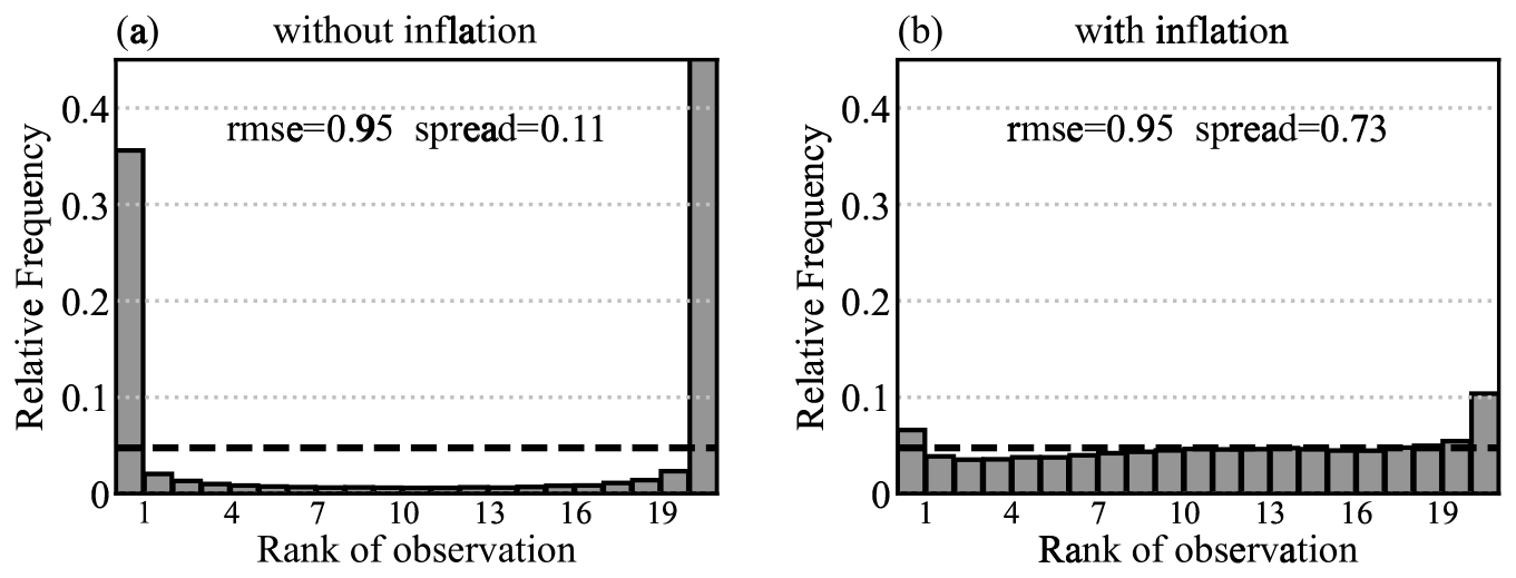
Figure 5 Talagrand diagram for T_2 m ensemble analysis without (a) and with (b) inflation in summer, averaged over all the outside stations.

Figure 6 shows the Talagrand diagram and reliability diagram for QQ_2 m and RH2m in both summer and winter. The ensemble for QQ_2 m in summer has a high resolution and reliability at different thresholds. Additionally, the flatness of the rank histogram indicates that the uncertainty has been estimated accurately. The conversion of RH2m involves temperature. To avoid the influence of temperature uncertainty on the variable conversion, only deterministic temperature observation is used in the humidity module. Therefore, this study does not account for the interplay effects between different variables. As a result, systematic biases in T_2 m within SIVA will propagate into RH2m, causing a dry bias in winter. In addition, the rank histogram and reliability for RH2m illustrate that the ensemble is underdispersive due to the neglect of variable conversion.

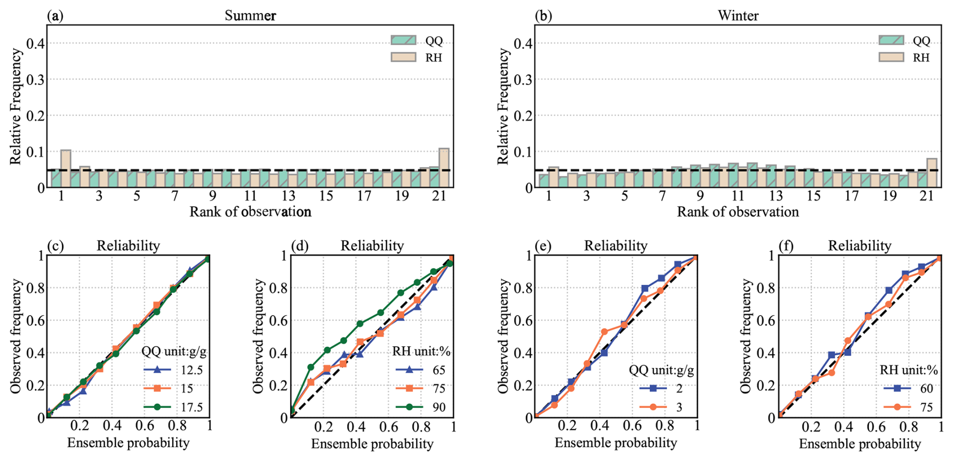
Figure 6 Talagrand (a, b) and reliability (c–f) diagrams for the ensemble analysis of QQ (g g⁻¹) and RH (%), averaged over all the test stations.

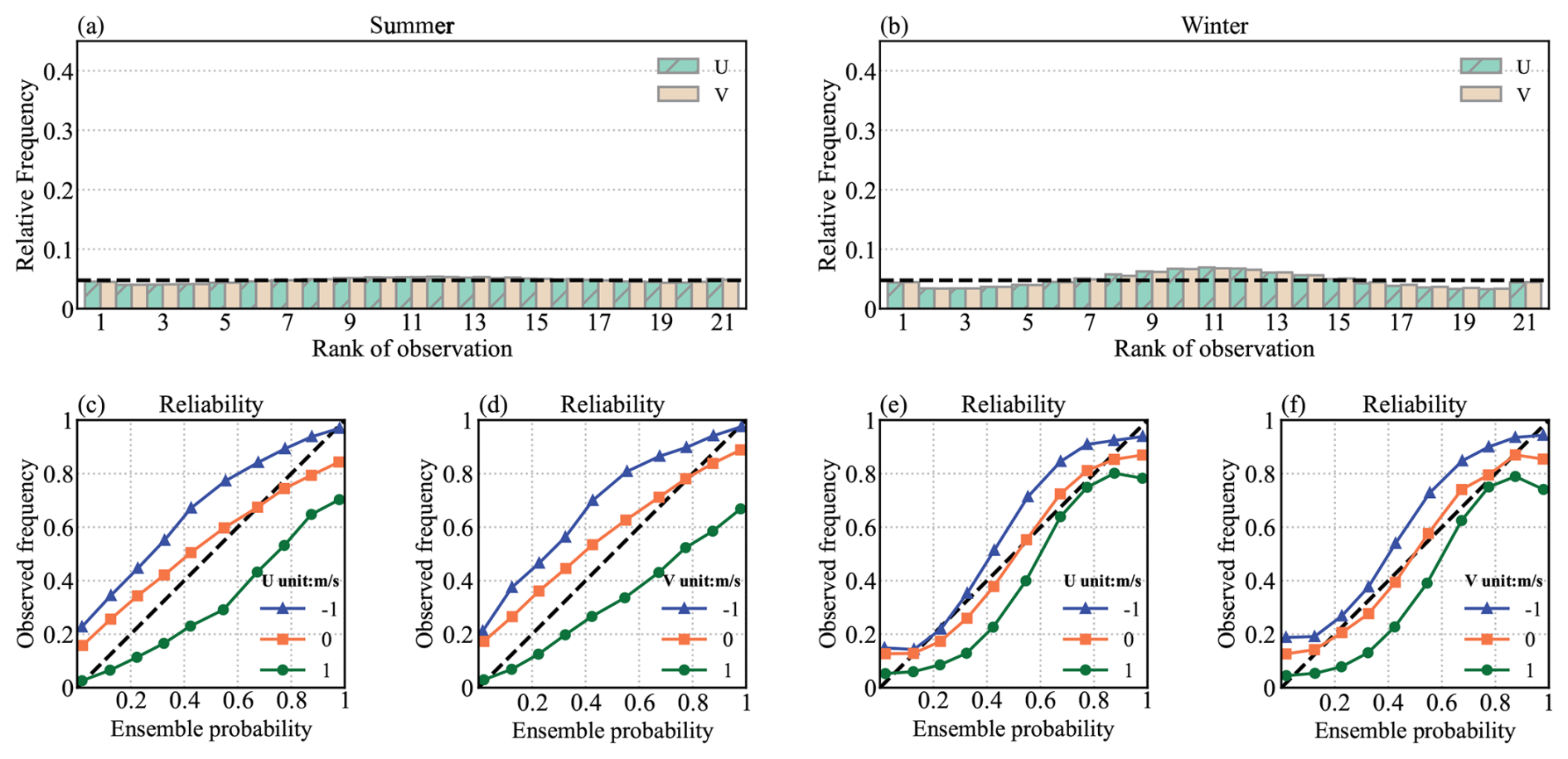
Figure 7 shows the Talagrand diagram and reliability diagram for wind components in summer and winter. A positive value of U_10 m (V_10 m) represents westerly (southerly) wind, while a negative value means easterly (northerly) wind. The bias for wind ensembles observed on the reliability curve is primarily caused by the representation of uncertainty in the wind direction. For example, when U_10 m is +1 m s⁻¹, the ensemble values may be −1 m s⁻¹, leading to significant bias due to the opposing wind direction. Although both U10 and V10 display a flat rank histogram, R_rs is less than 1 (Table 1) and the reliability curve does not match the diagonal line. These results suggest that the ensemble analysis of the wind components is less effective in reflecting uncertainty compared to T_2 m. A probable solution is to consider the impact of wind direction on observation data.

Figure 7 Same as Fig. 6 but for U_10 m and V_10 m (m s⁻¹).

4.2 Verification of nowcasting

Verifications of ensemble analysis demonstrate the reliability of the uncertainty estimation. The ensemble provides a spread at the initial time of nowcasting and exhibits a reasonable error that is consistent with the deterministic analysis. To evaluate the transmission effect of the spread in forecast extrapolation, the perturbed analyses are employed to compute ensemble nowcasting. Due to the range limitation in variable conversion, direct-ensemble nowcasting for RH2m is unfeasible. For wind, SIVA assigns a weight to the first guess based on an extrapolation step function. As the effectiveness of the extrapolation method gradually diminishes with the prolongation of the time steps, the weight assigned to the uncertainty information decreases when extrapolating to a lead time of 3 h. Hence, the ensemble nowcasting of wind is limited to a lead time of 2 h, while T_2 m and QQ_2 m are extrapolated up to a lead time of 6 h.

4.2.1 Ensemble bias and RMSE

Figure 8 shows that the bias and RMSE of the ensemble mean are nearly identical to those of deterministic nowcasting (hereafter called CNOW). As described in Sect. 4.1, the primary objective of this work is to quantify the uncertainty using a perturbation approach. The introduced perturbations are Gaussian-distributed with a mean of zero. In this context, the scores (bias and RMSE) of the ensemble mean should remain consistent with those of the deterministic reference. This ensures that the perturbations do not introduce additional biases while maintaining an accurate representation of uncertainty.

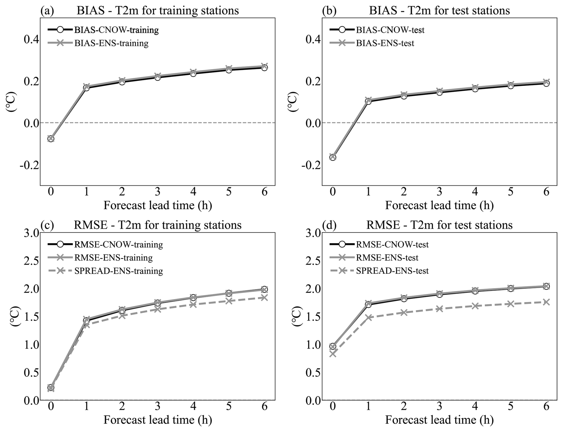
Figure 8 Bias (a, b) and RMSE (c, d) for the deterministic reference (black, CNOW, ◦) and ensemble mean (grey, ENS, ×) as a function of the forecast lead time. The ensemble spread is represented by the dashed grey line (×). These scores are averaged over all the training stations (a, c) or test stations (b, d) for August 2020.

The increases in the ensemble spread for both the training and test stations are consistent with those of the deterministic references and RMSE (Fig. 8). However, a certain degree of underdispersion can be observed as the lead times increase. One reason is that the extrapolation is based on the persistence of the first guess, which can only provide deterministic information. Although the first guess is perturbed at the initial time of the nowcasting, no additional noise is introduced into the forecasting. Therefore, the nowcasting uncertainty depends completely on the ensemble analysis. Furthermore, the perturbations in areas with test stations are amplified by the inflation factor. However, at the test stations, the difference between the spread and the RMSE is more pronounced than at the training stations. This phenomenon indicates that, although the inflation factor can amplify the spread in areas without stations, it does not fully capture the uncertainty from the complex interpolation in the analysis calculation. The ensemble nowcasting for specific humidity is also calculated, and due to its similarity to the temperature calculation framework the results are generally consistent.

For the wind components, the spread is consistent with the RMSE of the ensemble mean (Fig. 9). This could be attributed to the estimation of the lowest model layer through the divergence constraint after wind correction (3DRF), thereby avoiding dispersion attenuation caused by 2D interpolation. The ensemble nowcasting for the wind component shows a reliable spread that can be transmitted effectively without causing unusual increases in errors. However, when the lead time exceeds 3 h, the forecast is entirely represented by the first guess. Therefore, using an ensemble of first guesses is a promising approach for improving the uncertainty estimation of wind speed. Additionally, this may enhance the ability of the inflation factor to more comprehensively represent the interpolation uncertainty.

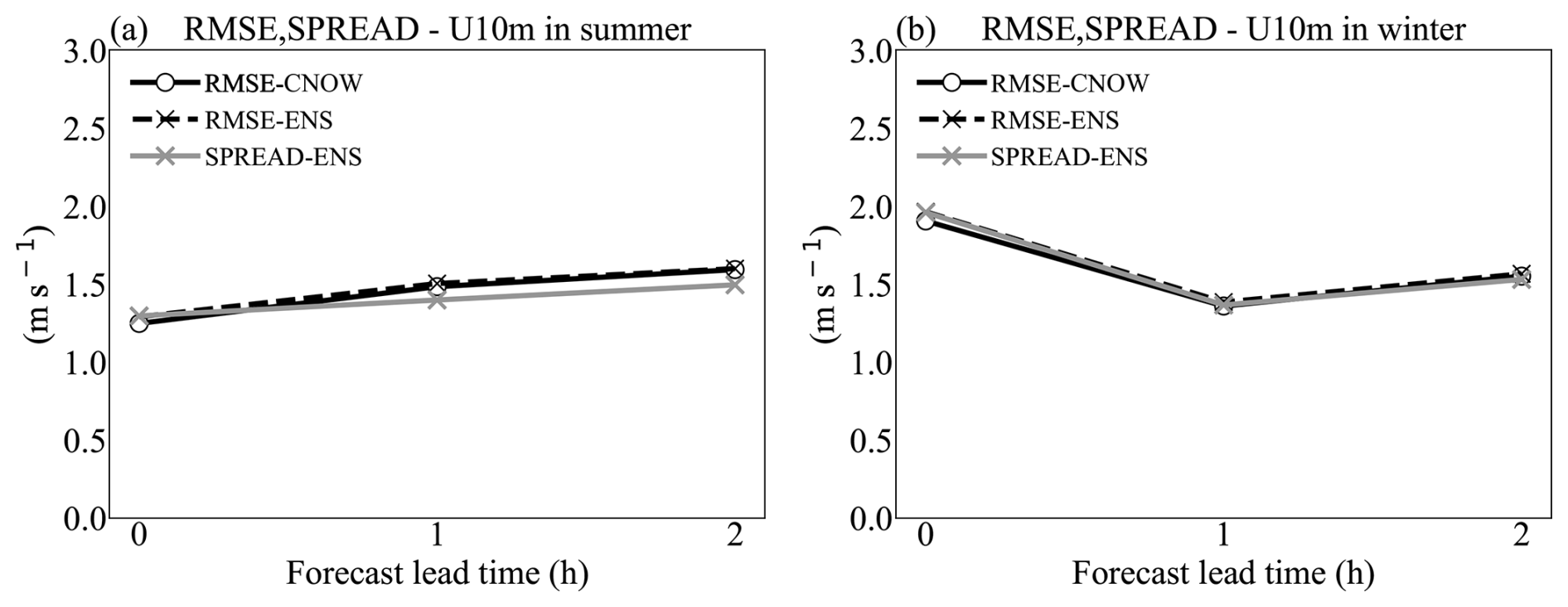
Figure 9 RMSE of the deterministic nowcasting (black, ◦), ensemble mean (black, ×), and ensemble spread (grey, ×) for U_10 m in both August 2020 (a) and February 2021 (b), averaged over all the test stations.

4.2.2 Probability scores

The reliability of T_2 m is evaluated in Fig. 10 in terms of the Talagrand diagram and reliability diagram, which are valid at the lead time +6 h. The verification reference is the observation at the test stations. The rank histogram displays a slight “L shape”, indicating a warm bias in the ensemble nowcasting. One reason is that the persistence of NWP is carried over into the extrapolation. At each time step, the NWP forecast adjusts by subtracting the previous step to represent the predictive trend of the variables, thereby converting the cold bias into a warm bias at the opposite site. In the reliability diagram, the thresholds are the quartile of the ranked temperature in both summer and winter. At each threshold, the ensemble probabilities align closely with the observed frequency. The high reliability and resolution of T_2 m ensemble nowcasting at a lead time of 6 h highlight the effectiveness of the proposed approach in quantifying the nowcast uncertainty.

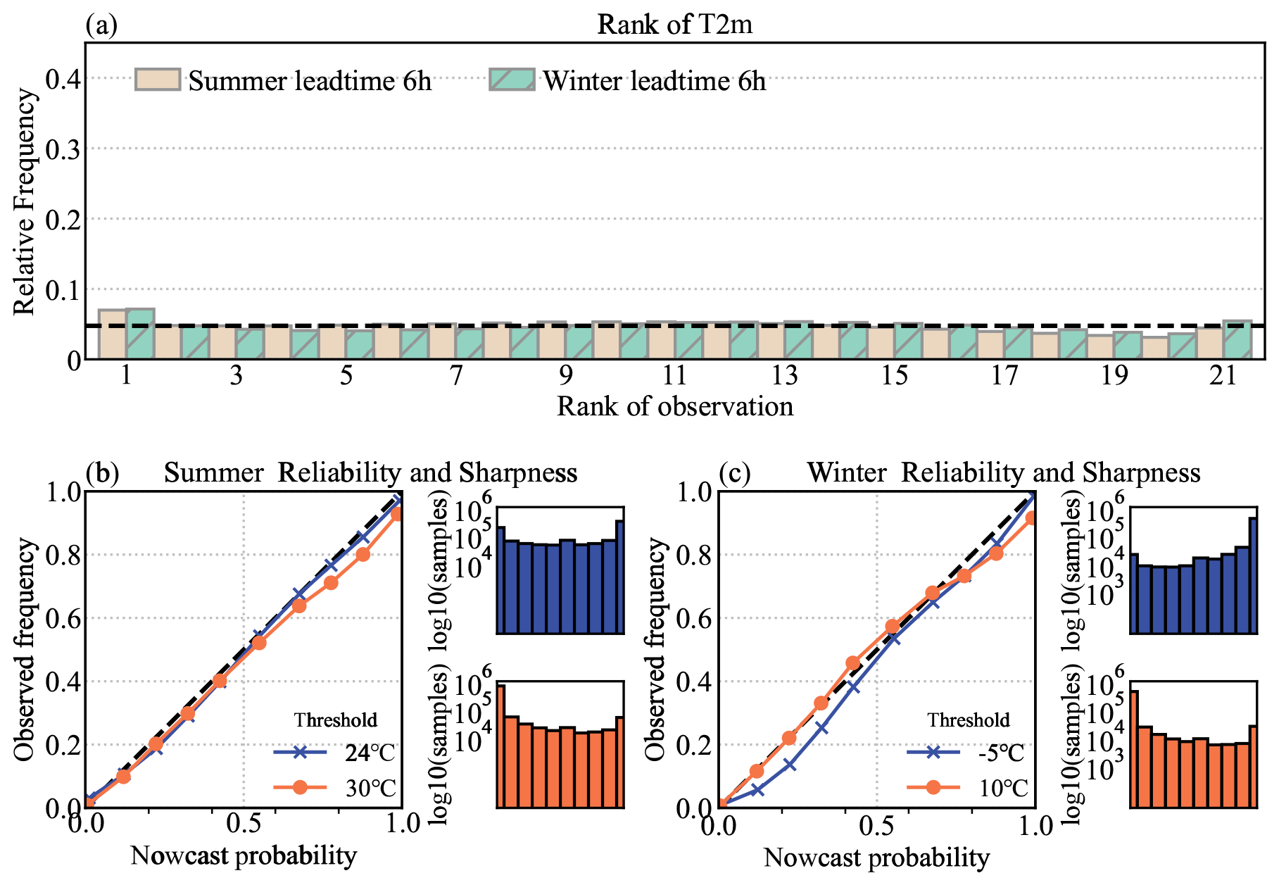
Figure 10 Talagrand (a) and reliability (b, c) diagrams for the ensemble nowcasting at a lead time of 6 h of T_2 m (°), verified over all the test stations.

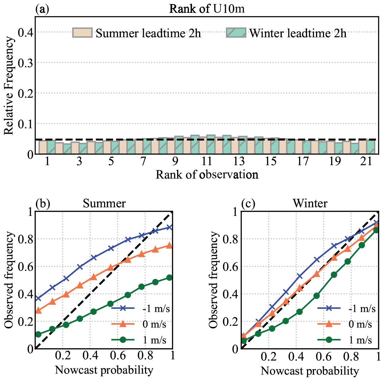
U_10 m and V_10 m have similar characteristics in the verification results. The verification of U_10 m shows that ensemble nowcasting performs with better reliability and resolution in summer compared to winter (Fig. 11). The evident bias for the summer U_10 m, as depicted on the reliability curve (Fig. 11b), suggests that ensembles struggle to capture wind direction uncertainty during periods of significant wind variability. This limitation arises from the lack of appropriate observational perturbations. In the calibration of wind components, vertical wind is used to calculate divergence in order to constrain the horizontal wind. Hence, the interpolation of wind differs from that of temperature. The divergence constraints cause the first-guess error to incorporate additional information in order to calibrate the first guess. For this reason, it is difficult to fully understand the impact of the perturbation on the observations. Consequently, the reliability of the wind components is lower than that of the temperature. Further research should address these difficulties by accounting for the impact of divergence constraints.

Figure 11 Same as Fig. 10 but for U_10 m (m s⁻¹).

5 Conclusion and discussion

This study proposes an efficient perturbation method to quantify the uncertainty of near-surface atmosphere analysis. Gaussian-distributed noise, generated based on the error characteristic, simulates the propagation of the uncertainty in the analysis computation. An inflation factor is computed to simulate the attenuation of perturbation dispersion during the interpolation process. The ensemble analysis offers a robust estimation of surface uncertainty at the initial time of nowcasting, aligning with the error increment observed in nowcasting extrapolation.

Adding noise to both observations and first guesses reflects the dispersion of the analysis error, which reflects the analysis uncertainty, especially in the areas without stations. For temperature, the spatial uncertainty caused by terrain can be addressed by incorporating the perturbed field with terrain information during interpolation. For humidity, its intrinsic correlation with temperature affects the estimation of the error uncertainty. For the wind components, the divergence constraint does not account for variations in perturbation information, resulting in an increased RMSE. Addressing this issue could be a focus of future improvements.

The ensemble analysis verification for all the variables demonstrates reliable representation of analysis uncertainty. However, wind components suffer from the influence of divergence constraints. Relative humidity is influenced by variable conversion processes, leading to an underdispersive ensemble.

The flat Talagrand diagrams illustrate that ensembles effectively estimate the probable range of true values. Introducing perturbations into analysis computation effectively quantifies the uncertainty of near-surface variables in both magnitude and spatial distribution. A limitation of the current method is that the inflation factor cannot represent the complexity of interpolation uncertainty. A possible improvement would be to see whether there are some predictors which could help inflation factors extrapolate perturbation information to the areas where there are truly no stations.

The ensemble analysis provides a reliable presentation of uncertainty at the initial time of nowcasting. The errors in ensemble nowcasting match those of deterministic nowcasting, and the growth of the ensemble spread aligns with the error growth trend in nowcasting extrapolation. Since this method does not account for the uncertainty derived by NWP systematic errors and the relativity of different variables, the ensemble nowcasting is slightly underdispersive.

The perturbed first-guess errors, along with the spread and error of the ensemble, are associated with the analysis errors observed at the test stations. The perturbation method in this study addresses the challenge in accurately representing the uncertainty of near-surface deterministic analysis. This method enhances the estimation of near-surface analysis uncertainty for both nowcasting applications and ensemble nowcasting development. Further improvements could involve considering the uncertainty in estimating the first-guess error of multi-source NWP in order to obtain a more comprehensive spatial uncertainty representation.

Appendix A: Case of generating temperature perturbation

Listing A1 presents how to generate perturbation for both observations and NWP. This case is for 2 m temperature, while the specific humidity and wind components have similar processes. The input files sta_inf and grid_inf are the example temperature data and the corresponding standard deviation of the first-guess error. Due to the confidentiality agreement, these files only include the temperature value. The variable inflation in grid_inf is the inflation factor which is used to rescale the perturbed NWP. Since the standard deviation of the perturbation generated by the function numpy.random.normal exists offset, the factors sc_sta and sc_grid are used to ensure that the scale of the perturbation is consistent with the scale of the first-guess error.

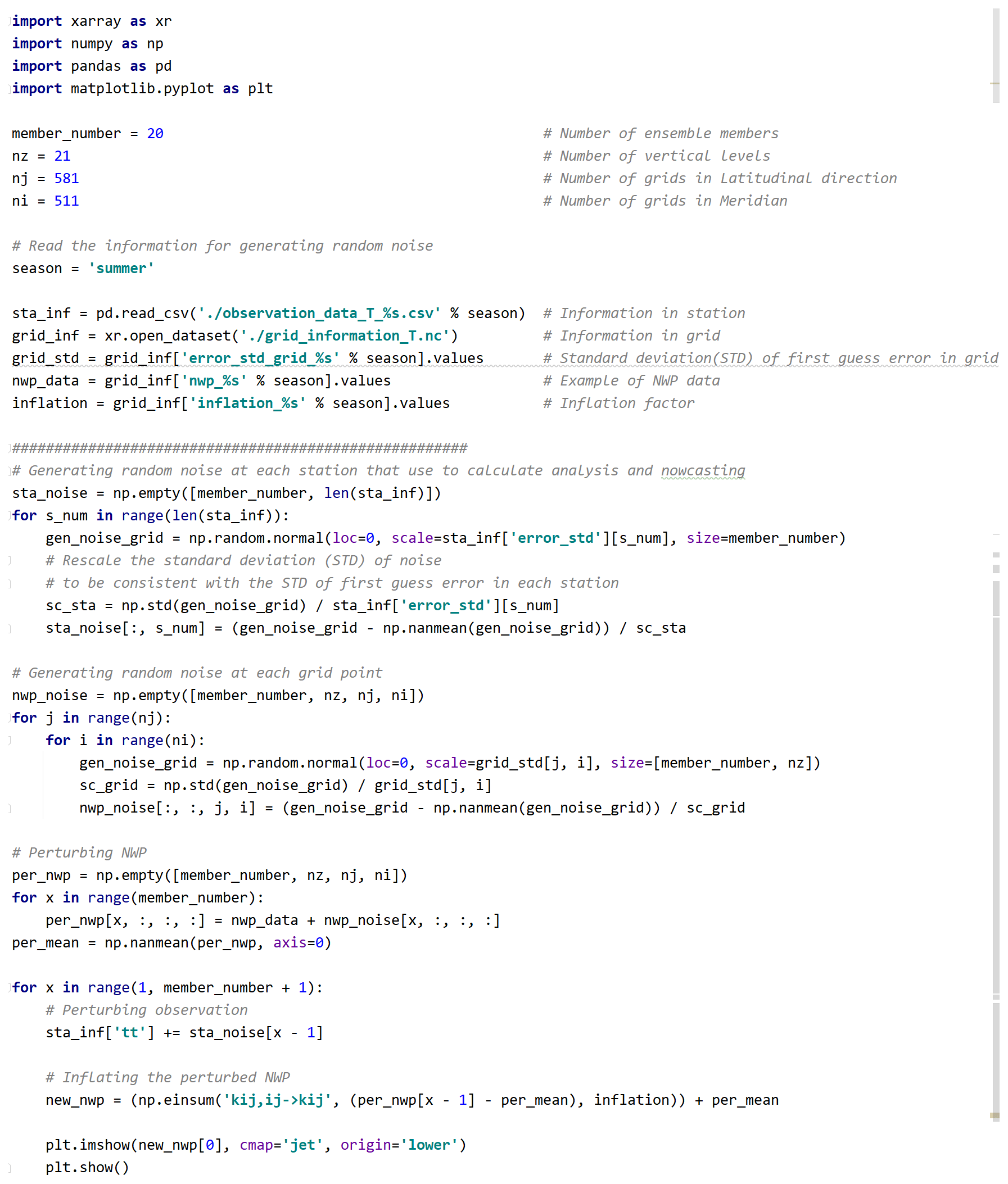
Listing A1 Processes of generating random perturbation and rescaling the perturbed NWP using the inflation factor.