the Creative Commons Attribution 4.0 License.
the Creative Commons Attribution 4.0 License.
 | 08 Dec 2023
Data assimilation for the Model for Prediction Across Scales – Atmosphere with the Joint Effort for Data assimilation Integration (JEDI-MPAS 2.0.0-beta): ensemble of 3D ensemble-variational (En-3DEnVar) assimilations
Zhiquan Liu
Chris Snyder
Byoung-Joo Jung
Craig S. Schwartz
Junmei Ban
Steven Vahl
Yali Wu
Ivette Hernández Baños
Yonggang G. Yu
Soyoung Ha
Yannick Trémolet
Thomas Auligné
Clementine Gas
Benjamin Ménétrier
Anna Shlyaeva
Mark Miesch
Stephen Herbener
Emily Liu
Daniel Holdaway
Benjamin T. Johnson
An ensemble of 3D ensemble-variational (En-3DEnVar) data assimilations is demonstrated with the Joint Effort for Data assimilation Integration (JEDI) with the Model for Prediction Across Scales – Atmosphere (MPAS-A) (i.e., JEDI-MPAS). Basic software building blocks are reused from previously presented deterministic 3DEnVar functionality and combined with a formal experimental workflow manager in MPAS-Workflow. En-3DEnVar is used to produce an 80-member ensemble of analyses, which are cycled with ensemble forecasts in a 1-month experiment. The ensemble forecasts approximate a purely flow-dependent background error covariance (BEC) at each analysis time. The En-3DEnVar BECs and prior ensemble-mean forecast errors are compared to those produced by a similar experiment that uses the Data Assimilation Research Testbed (DART) ensemble adjustment Kalman filter (EAKF). The experiment using En-3DEnVar produces a similar ensemble spread to and slightly smaller errors than the EAKF. The ensemble forecasts initialized from En-3DEnVar and EAKF analyses are used as BECs in deterministic cycling 3DEnVar experiments, which are compared to a control experiment that uses 20-member MPAS-A forecasts initialized from Global Ensemble Forecast System (GEFS) initial conditions. The experimental ensembles achieve mostly equivalent or better performance than the off-the-shelf ensemble system in this deterministic cycling setting, although there are many obvious differences in configuration between GEFS and the two MPAS ensemble systems. An additional experiment that uses hybrid 3DEnVar, which combines the En-3DEnVar ensemble BEC with a climatological BEC, increases tropospheric forecast quality compared to the corresponding pure 3DEnVar experiment. The JEDI-MPAS En-3DEnVar is technically working and useful for future research studies. Tuning of observation errors and spread is needed to improve performance, and several algorithmic advancements are needed to improve computational efficiency for larger-scale applications.
- Article
(4254 KB) - Full-text XML
- BibTeX
- EndNote


Liu et al. (2022) introduced a new data assimilation (DA) system for the Model for Prediction Across Scales – Atmosphere (MPAS-A; Skamarock et al., 2012) that is built on the Joint Effort for Data assimilation Integration (JEDI; Trémolet and Auligné, 2020) software framework, called JEDI-MPAS. Liu et al. (2022) demonstrated JEDI-MPAS for global 3D ensemble-variational (3DEnVar) DA to produce a deterministic (single-state) analysis of the atmosphere. When approximating flow-dependent background error covariances (BECs) in 3DEnVar, they used 20-member ensembles of MPAS-A forecasts that were initialized from initial conditions used by the National Centers for Environmental Prediction (NCEP) Global Ensemble Forecast System (GEFS) (Zhou et al., 2017).
It would be preferable for a myriad of research applications that the ensemble used in the DA be generated by JEDI-MPAS itself so that it is consistent with the details – such as the characteristics of the observing network – of a given application. Here we evaluate using an ensemble of data assimilations (EDA), implemented generically in JEDI and available for any forecast model with JEDI interfaces, to generate ensemble initial conditions for JEDI-MPAS. Our first EDA implementation is for an ensemble of 3DEnVars (En-3DEnVar) because it requires very few modifications to the EnVar algorithm previously described by Liu et al. (2022). A major attraction of EDA based on variational algorithms is that most technical or algorithmic improvements targeted for deterministic DA will directly translate to the ensemble system.
The technique that we term EDA involves conducting an ensemble of independent analysis and forecast steps in each cycle. Each member ingests perturbed versions of the available observations during its assimilation step. This technique was proposed and tested by Houtekamer and Derome (1995), who called the approach “OSSE-MC”. Subsequent studies employed EDA (under other names) to generate analysis ensembles for ensemble forecasting systems (Houtekamer et al., 1996; Hamill et al., 2000), for estimating forecast-error statistics for DA covariance modeling (Fisher, 2003; Zagar et al., 2005; Berre et al., 2006), and in “stochastic” ensemble Kalman filters (EnKFs) (Houtekamer and Mitchell, 1998; Burgers et al., 1998; and many subsequent papers).
Variationally based EDA was first implemented operationally as an ensemble of 4D variational (En-4DVar) minimizations at Météo-France (Berre et al., 2007; Desroziers et al., 2008; Berre and Desroziers, 2010), and then at the European Centre for Medium-Range Weather Forecasts (Isaksen et al., 2010). The UK Met Office later replaced its local ensemble transform Kalman filter (LETKF) with an ensemble of hybrid 4DEnVars (En-4DEnVar) in their ensemble prediction system through extensive efforts (Bowler et al., 2017a, b; Lorenc et al., 2017) and following multiple motivations: code maintenance is reduced via shared software with their deterministic 4DVar, there is an improved capability to use more advanced model-space localization techniques (i.e., Lorenc, 2017), the En-4DEnVar produced faster and more realistic ensemble spread growth in forecasts than LETKF (Bowler et al., 2017b), En-4DEnVar perturbations used as flow-dependent BECs improved forecasts in their deterministic hybrid 4DVar system compared to LETKF perturbations (Bowler et al., 2017a), and En-4DEnVar is cheaper than an alternative En-4DVar. On the topic of model-space localization, multiple authors have documented its use with an EnKF since 2017 (Bishop et al., 2017; Lei et al., 2018).
There are numerous techniques besides variationally based EDA for generating ensembles of initial conditions, including 4D ensemble Kalman smoothers (Evensen, 2003). In particular, a relatively mature EnKF for MPAS exists (Ha et al., 2017), which is based on the Data Assimilation Research Testbed (DART; Anderson et al., 2009); we call this system MPAS-DART. Although not a focus of this paper, the MPAS-DART EnKF is a useful benchmark for initial evaluations of the JEDI-MPAS En-3DEnVar, and we present companion results from MPAS-DART for many aspects of JEDI-MPAS performance.
While variationally based EDA poses a large potential benefit of increased skill via reuse of 4D algorithms, it also incurs more computational overhead per member than many EnKF algorithms. There are numerous EDA algorithm advances in previous works to alleviate some of the added cost compared to the EnKF, such as separating the update of the ensemble mean and perturbations and using simpler, cheaper configurations for the perturbation update (Buehner et al., 2017; Lorenc et al., 2017), block minimization methods (Mercier et al., 2018), and advanced in-memory storage and communication strategies for the numerous ensemble perturbations (Arbogast et al., 2017). We do not consider such enhancements in this paper, though they may certainly be helpful in the future.
The outline of the paper is as follows. In Sect. 2 we briefly describe the JEDI-MPAS En-3DEnVar implementation and the MPAS-DART EnKF, both of which are used in our experiments. In Sect. 4, we compare the 6 h ensemble forecast statistics produced with the JEDI-MPAS En-3DEnVar and the MPAS-DART EnKF across 1 month of cycling on the MPAS-A quasi-uniform 60 km mesh. Although we do not present a general comparison of an EnKF and EDA, there are very few comparisons in the literature (e.g., Hamrud et al., 2015; Bonavita et al., 2015), and this work gives another data point. In Sect. 5, we use the 6 h forecasts initialized from the MPAS-DART EnKF and JEDI-MPAS EDA analyses as ensemble BECs in several dual-mesh “30 km–60 km” (i.e., 30 km outer loop and 60 km inner loops) 3DEnVar deterministic cycling experiments to show the utility of the EDA in producing flow-dependent BECs. Finally we finish with conclusions and a future outlook for JEDI-MPAS ensemble DA in Sect. 6.
2.1 JEDI-MPAS EDA
Liu et al. (2022) described the 3DEnVar algorithm implemented in JEDI, and thus JEDI-MPAS, following Lorenc (2003) and Buehner (2005). We utilize the same algorithm and software implementation in the En-3DEnVar and in subsequent deterministic 3DEnVar experiments. In the EDA there are Ne independent cost functions, where the ith EDA cost function is evaluated at the ith background state xb,i,
The vectors ϵi are realizations of the random observation error , where R is the observation error covariance matrix, and the ensemble mean of the realizations is removed so that . Removing the perturbation bias is standard practice to avoid biasing the posterior, although doing so alters the distribution of the perturbations. The observation operator, h, simulates model-equivalent observations given the state, x. In each outer iteration of a truncated Gauss–Newton minimization (Lawless et al., 2005), an inner-loop minimization uses a linear approximation of Eq. (1) to determine the analysis increment. The increment is added to the current guess of x, beginning at xb,i in the first outer iteration.
As described by Liu et al. (2022), the ith BEC, Bi in Eq. (1), is a weighted sum of the climatological background error covariance Bc and the member-specific sample ensemble covariance Be,i, i.e.,
where βc and βe are scalar weights, with . βc, βe, and Bc are identical for all EDA members. denotes the Schur product (element by element) of the localization matrix L and Be,i. The member-specific Be,i allows for self-exclusion, described in Sect. 2.1.1. Note that L is a correlation matrix with diagonal elements being 1 and off-diagonal elements smaller than 1 that reduce to 0 for a certain distance between two model grid points. Therefore, the localization matrix reduces spurious correlations in Be,i caused by sampling errors associated with a limited ensemble size. The only difference between the description above for EDA cycling and deterministic cycling is that the latter only has one background state, the observations are not perturbed, and the BEC only has one realization based on all Ne members.
As described by Liu et al. (2022), the analysis variables are temperature (T), horizontal wind components (U, V), surface pressure (Ps), and specific humidity (Qv). One difference from Liu et al. (2022) is that the hydrostatic balance constraint in the analysis increment stage is no longer applied directly to the full analysis variables. Instead, an incremental form of the hypsometric equation is used to approximate the dry-air density (ρd) and 3D pressure (P) increments from the increments in T, Ps, and Qv. The hypsometric equation is linearized around a hydrostatic state constructed using the previous outer iteration analysis, xi, of T, Ps, and Qv. After the DA minimization is complete, the analysis state is transformed to the MPAS-A prognostic variables during the model initialization before the model's time integration.
The ensemble BEC, Be, is represented by prior perturbations (before assimilation) in those same analysis variables with respect to the prior ensemble mean. As described in Jung et al. (2023), Bc is constructed by applying linear transformations that yield the analysis variables from stream function, velocity potential, and the “unbalanced” contributions to temperature and surface pressure together with the assumption that background errors in those underlying variables are mutually independent and have known isotropic covariances (Derber and Bouttier, 1999). Bc is implemented via generic JEDI interfaces to the Background error on Unstructured Mesh Package (BUMP; Ménétrier, 2020).
2.1.1 Self-exclusion
As first shown by Houtekamer and Mitchell (1998), updating an ensemble of forecasts using an assimilation scheme based on the sample covariances of that same ensemble, as in En3DEnVar for example, leads to an analysis ensemble with too little spread when compared to the errors in the analysis mean. To counteract this systematic bias in the update, they proposed splitting the ensemble into subsets and updating members in a given subset using the sample covariance from members in the other subsets.
In the limit that the subsets contain a single member, each member i in the EDA will use in the cost function (1) a different, flow-dependent BEC Be,i, obtained by omitting , the ith ensemble perturbation, from the computation of Be,i, where is the ensemble mean. Sacher and Bartello (2008) and Mitchell and Houtekamer (2009) showed with small toy problems that this approach causes the posterior ensemble spread to overestimate the root-mean-square error (RMSE) of the posterior ensemble mean.
Bowler et al. (2017b) called the removal of δxi from Be,i “self-exclusion”, applying it to an En-4DEnVar, while Buehner (2020) called it “cross-validation”, applying it to an LETKF. Bowler et al. (2017b) and Buehner (2020) both found that self-exclusion reduced the spread reduction that occurred during the DA procedure going from background ensemble to the analysis ensemble. Even so, Bowler et al. (2017b) found that applying self-exclusion necessitated the use of more relaxation than when not using self-exclusion (see Sect. 2.1.2 for a definition of relaxation). Self-exclusion is applied in the JEDI-MPAS EDA experiment described in Sect. 4.
2.1.2 Ensemble spread tuning
The EDA update described above will systematically underestimate the analysis uncertainty to some degree, despite employing multiple techniques to reduce the detrimental effects of sampling error: covariance localization in the ensemble BEC, hybridization with a static BEC, and self-exclusion. More important, the ensemble forecasts in JEDI-MPAS do not at present account for model error, so even if the analysis ensemble is perfectly representative of the statistics of analysis error the ensemble forecast will be underdispersive. Both effects will also accumulate over successive forecast–analysis cycles. For these reasons, it is essential that JEDI-MPAS include some method for tuning the overall ensemble spread.
There are many approaches for tuning ensemble spread to ensure stable cycling of the ensemble-dependent DA and forecast system. In the relaxation to prior perturbations (RTPP; Zhang et al., 2004) method, the analysis perturbation for member i, δxa,i, is replaced by a weighted sum of δxa,i and δxb,i with a scalar weight αRTPP, i.e.,
Thus, the relaxed ensemble perturbations take on some of the observationally constrained analysis perturbations, δxa,i, and the forecast-model-driven background perturbations, δxb,i. In JEDI-MPAS, RTPP is carried out via a standalone executable, one which inherits from a generic implementation in the JEDI Object-Oriented Prediction System (OOPS) for the RTPP application.
Whitaker and Hamill (2012) proposed an alternative to RTPP called relaxation to prior spread (RTPS), which relaxes the spread of the analysis ensemble toward the background ensemble spread instead of relaxing the perturbations. The underpinning of RTPS is the spread change ratio, s, whose jth element, associated with a given grid cell and analysis variable, is calculated as
where σb,j and σa,j are the prior and posterior ensemble sample standard deviations (spreads). RTPS operates independently for each j using a Schur product,
It is common practice to combine RTPP with RTPS (e.g., Bowler et al., 2017b) or with multiplicative inflation or to adapt α at each DA cycle (e.g., Kotsuki et al., 2017). Here we only use RTPP with a fixed global α throughout all DA cycles as a means of providing an initial JEDI-MPAS EDA functionality to the community. There remain many opportunities for improving ensemble spread in future work.
2.1.3 Implementation
In the EDA experiment presented here, each member is treated with a fully independent execution of the JEDI-MPAS Variational application (https://jointcenterforsatellitedataassimilation-jedi-docs.readthedocs-hosted.com/en/latest/inside/jedi-components/oops/applications/variational.html, last access: 28 October 2022). OOPS contains implementations for generic model-independent applications in JEDI. The generic OOPS Variational application can be used to conduct 3DVar, 3DEnVar, 4DEnVar, and 4DVar (for models with linearized tangent and adjoint descriptions), as well as applicable hybrid variants thereof. Only 3DVar, 3DEnVar, 4DEnVar, and hybrid variants are enabled in the JEDI-MPAS model-specific Variational executable at this time. Self-exclusion is achieved in En-3DEnVar simply by removing each member's own background state from a list of ensemble members in the Variational application configuration.
The ensemble forecasts and EDA are conducted via our open-source MPAS-Workflow (https://github.com/NCAR/MPAS-Workflow, last access: 8 March 2023), which uses the Cylc general purpose workflow manager (Oliver et al., 2019) v7.8.3 to orchestrate tasks written in a combination of c-shell and Python scripts. MPAS-Workflow automatically constructs Variational application configuration files in YAML (yet another markup language) format for each cycle. At the time of writing, MPAS-Workflow only operates on the Cheyenne HPC (high-performance computer) managed by the National Center for Atmospheric Research's (NCAR) Computational and Information Systems Laboratory (CISL). MPAS-Workflow handles a small set of use cases specific to the NCAR Microscale and Mesoscale Meteorology (MMM) Laboratory. Although it is not yet designed for general purpose use, this open-source repository might serve to instruct others on how to run JEDI-MPAS and MPAS-A together.
The source code used for our experiments is provided in the JEDI-MPAS 2.0.0-beta release version, as described in the “Code and data availability” section.
2.2 EAKF in MPAS-DART
To assess the credibility of our newly developed JEDI-MPAS EDA system, an ensemble adjustment Kalman filter (EAKF; Anderson, 2001, 2003; Anderson and Collins, 2007) implemented within the “Manhattan” version of DART (Anderson et al., 2009) is also used to produce analyses. DART is a mature software platform for ensemble-based DA and has been interfaced with MPAS-A (Ha et al., 2017). DART can perform both stochastic and deterministic EnKF algorithms, where only the former perturbs observations. When background and observation error distributions are near-Gaussian, the use of perturbed observations is known to degrade the quality of the ensemble-mean analysis relative to that produced by deterministic filters (Anderson, 2001; Whitaker and Hamill, 2002) and a theoretically similar deterministic variationally based EDA (Bowler et al., 2012). On the other hand, as the forecast model and observation operators become increasingly nonlinear, there is evidence that an EDA with perturbed observations avoids some pathological behaviors that appear in deterministic EnKFs (Lawson and Hansen, 2004; Anderson, 2010; Lei et al., 2010; Anderson, 2020).
As a deterministic square-root variant of the EnKF, the EAKF has many differences from the EDA algorithm described in Sect. 2.1. The primary difference is that EAKF does not perturb observations; all members assimilate an identical realization of a given observation (i.e., the measured observation). Another technical difference is that the EAKF assimilates observations one at a time, whereas variational minimizations assimilate all observations simultaneously. Moreover, while 3DEnVar applies covariance localization in model space, the EAKF applies localization to observation–observation and observation–state covariances, which may be suboptimal for assimilation of radiance observations (Campbell et al., 2010; Lei et al., 2018). Additionally, the EAKF does not employ self-exclusion (Sect. 2.1.1) to compute unique BECs for each ensemble member, and there are also differences regarding posterior relaxation between EDA and the EAKF (described in Sect. 4.1). Finally, MPAS's interface with DART does not use a hydrostatic pressure constraint on analysis increments, unlike JEDI-MPAS's variational algorithm (Sect. 2.1).
There are clearly many differences between the En-3DEnVar implemented in JEDI-MPAS and the EAKF in MPAS-DART. Moreover, neither system has been thoroughly tuned, and DART has many capabilities that we do not exercise, including sophisticated inflation and localization options. We therefore do not attempt to attribute differences between their performances to specific settings or parameters. Instead, we view MPAS-DART as a convenient baseline against which to compare the robustness and validity of our newly developed EDA implementation within JEDI-MPAS.
3.1 MPAS-A model
MPAS-A is a non-hydrostatic model discretized on an unstructured centroidal Voronoi mesh in the horizontal with C-grid staggering of the state variables and works for both global and regional applications (Skamarock et al., 2012, 2018). Herein we present results using two different MPAS-A quasi-uniform meshes, 60 km (163 842 horizontal columns) and 30 km (655 362 columns). All time integrations for the 60 km mesh use a 360 s time step, while those for the 30 km mesh use a 180 s time step. Additional sensitivity experiments are described that utilized the quasi-uniform 120 km mesh (40 962 columns) with a 720 s time step. All meshes utilize 55 vertical levels with a 30 km model top and the “mesoscale reference” physics suite, as described by Liu et al. (2022).
In almost all respects, the same modified version of MPAS-A version 7.1 that was used by Liu et al. (2022) is used here. Some minor code modifications are included in the JEDI-MPAS 2.0.0-beta release version, as described in the “Code and data availability” section.
3.2 Observations
All experiments assimilate the same set of observations. We convert netCDF-formatted observation diagnostic files from the Gridpoint Statistical Interpolation (GSI; Shao et al., 2016) system (i.e., “GSI-ncdiag”) to a format that can be read by the JEDI Interface for Observation Data Access (IODA; Honeyager et al., 2020). For in situ observations, we assimilate sondes (temperature, virtual temperature, zonal and meridional wind components, specific humidity), aircraft (temperature, zonal and meridional wind components, specific humidity), and surface pressure. For non-radiance remote observations, we assimilate satellite atmospheric motion vectors (AMVs, zonal and meridional wind components) and global navigation satellite system and global positioning system radio occultation (collectively referred to as GNSSRO herein) refractivity.
We assimilate clear-sky microwave radiances as brightness temperature from six Advanced Microwave Sounding Unit-A (AMSU-A) sensors aboard NOAA-15, NOAA-18, NOAA-19, AQUA, MetOp-A, and MetOp-B. We only assimilate channels 5 to 9 because higher-peaking channels are sensitive to stratospheric regions that are above the 30 km model top and thus cannot be simulated correctly. Additionally, some AMSU-A channels are removed following sensitivity experiments that showed larger RMSEs or lower quality in 6 h forecasts: NOAA-19 channel 8; AQUA channels 5, 6, and 7; MetOp-A channels 7 and 8; and MetOp-B channels 5, 6, and 7.
The GSI-ncdiag files include brightness temperature bias correction, which is calculated using variational bias correction (VarBC) in GSI to correct for fluctuations in instrument bias. We add those pre-computed bias corrections directly to the observed brightness temperature before reading the IODA-formatted observations into JEDI-MPAS. Similarly, observation error standard deviations (square root of diagonal of R) come directly from the GSI-ncdiag files for most observation types. The only exceptions are for GNSSRO and satellite AMVs. The GNSSRO refractivity errors are calculated online within the JEDI unified forward operator (UFO; Honeyager et al., 2020) using a height-dependent parameterization ported from GSI.
Table 1Observation error standard deviation versus pressure for satellite AMVs.

In early sensitivity experiments, we determined that the observation errors for AMVs provided in GSI-ncdiag files were much larger than the RMSE of JEDI-MPAS background innovations, , and that the observations were much denser than either of the 30 or 60 km meshes. We opt to reduce the correlations between dense observations by thinning them horizontally. Both AMVs and radiances are thinned on a 145 km global Gaussian mesh. Also, we opt to decrease the prescribed AMV observation errors according to the pressure-dependent values shown in Table 1, with linear interpolation between the pressures shown and following the same parameterization as an early Joint Center for Satellite Data Assimilation (JCSDA) near-real-time prototype (Greg Thompson, personal communications, 2022). As is discussed in the context of the results, there are many opportunities still to optimize the observation errors for the JEDI-MPAS cycling system, but that is not the major focus of this work.
We use a quality control (QC) check for all observations that allows for maximum “PreQC” quality flags (as provided in the GSI-ncdiag files) of 0 and 3 for radiance and non-radiance instruments, respectively. PreQC includes various checks for raw data quality, as well as background innovation checks from GSI based on its own background state. We additionally filter observation locations and variables that exceed a 3σo background check (i.e., the observation error normalized absolute innovation must satisfy to be assimilated). Surface pressure locations are removed when the model elevation and observing station elevation differ by more than 200 m. Also, the surface pressure forward operator includes a height correction following the appendix of Ingleby (2013).
4.1 Setup
We conduct two ensemble cycling experiments with nearly identical settings. One experiment uses the JEDI-MPAS EDA (EDA), and the other experiment uses the MPAS-DART EAKF (DART). Both experiments use 80 initial ensemble backgrounds generated by integrating 4 sets of 20 MPAS-A forecasts. The 4 forecast sets are initialized from 20-member GEFS initial conditions (i.e., 0 h forecasts) valid at 00:00, 06:00, 12:00, and 18:00 UTC on 14 April 2018. Thus the first cycle background ensemble at 00:00 UTC on 15 April 2018 is comprised of 24, 18, 12, and 6 h forecasts on the 60 km mesh.
Both ensemble experiments alternate between data assimilation and an ensemble of 6 h forecasts at each cycle until 18:00 UTC on 14 May 2018, ending with a final forecast valid at 00:00 UTC on 15 May 2018. This 1-month experimental period is too short to draw broad conclusions but is sufficient to demonstrate the new En-3DEnVar capability. The results that follow in Sect. 4.2 reflect statistics calculated from 00:00 UTC on 17 April 2018 to 18:00 UTC on 14 May 2018 (inclusive) to allow 2 d for spin-up of characteristic errors. The unique aspects of the EDA and DART experiments follow.
Each EDA variational minimization uses a single outer-loop iteration and 60 inner-loop iterations. The ensemble BEC localization uses fixed-length scales of 1200 and 6 km in the horizontal and vertical dimensions, respectively. Prior to conducting the 60 km experiments presented here, we carried out 1-month EDA sensitivity experiments on the 120 km mesh to determine the impacts of self-exclusion and RTPP. We found that using self-exclusion increased background ensemble spread for a fixed αRTPP and improved forecast verification scores compared to not using self-exclusion. Therefore, we use self-exclusion without further sensitivity study in the 60 km EDA experiment.
Among selected αRTPP, varying from 0.5 to 0.95 in 0.05 steps, we found that αRTPP=0.80 yielded the best 1 to 10 d forecasts in 120 km sensitivity tests with 20 ensemble members. Those forecasts were initialized by the mean of the 20-member analysis ensembles at 00:00 and 12:00 UTC from 15 April to 4 May 2018. We also generally found improvement when increasing ensemble size from 20 members to 80 members while using αRTPP=0.80, with some saturation of forecast quality seen with only 40 members. As Bowler et al. (2017b) described, αRTPP can be decreased when increasing ensemble size because sampling error is reduced. Similarly, inflationary measures can be reduced when decreasing mesh spacing because sub-grid-scale model error is reduced, and resolved physics are more active, mitigating underdispersiveness in ensemble forecasts. Therefore we executed two different 20-member 10 d EDA experiments on the 60 km mesh with αRTPP=0.4 and αRTPP=0.7. Their mean background RMSE was much less sensitive to the relaxation coefficient than were the 20-member experiments on the 120 km mesh. Therefore, we chose αRTPP=0.7 for the 80-member 60 km EDA experiment, even if it may not be an optimal setting.
The DART experiment is identical to the EDA experiment in terms of initialization, cycling period (6 h), and cycling duration. In addition, the EAKF uses the same 1200 km horizontal and 6 km vertical localization length scales as EDA, although localization in DART is in observation space rather than model space (see Sect. 2.2). Although Greybush et al. (2011) found that optimal observation-space localization lengths ought to be shorter than those in model space, careful tuning of the DART experiment was not our focus. DART uses RTPS with αRTPS=1.0 to maintain ensemble spread throughout cycling.
For observations, DART uses the JEDI-MPAS model-specific implementation of the OOPS HofX3D application (https://jointcenterforsatellitedataassimilation-jedi-docs.readthedocs-hosted.com/en/latest/inside/jedi-components/oops/applications/hofx.html, last access: 28 October 2022) to apply forward operators for each ensemble member, assign observation errors, and perform quality control and observation thinning. The output of HofX3D is then ingested into MPAS-DART, bypassing DART's own forward operators and observation processing capabilities.
Given the coupling of HofX3D to MPAS-DART, both EDA and DART utilize identical observations possessing identical observation errors (Sect. 3.2). However, there is one subtle difference regarding observation QC filtering. The background check for all members in DART is based on the prior ensemble mean, whereas the background check in EDA is applied independently to each ensemble member before the observations are perturbed. That difference, coupled with differences in algorithm, localization, and inflationary measures between EDA and DART (Sect. 2), means that throughout the month of cycling the two experiments assimilate slightly different observations because different observations could fail the background check between experiments. Nonetheless, any differences in assimilated observations reflect differences in the assimilation algorithms and their particular settings rather than the observation rejection.
Throughout this section and Sect. 5, comparisons are made to initial conditions (referred to herein as “analyses”) used in the NCEP Global Forecasting System (GFS). The GFS analyses are transformed to the same mesh used to produce forecasts (e.g., 60 or 30 km) via MPAS-A's initialization procedures. GFS is a well-tuned operational forecast system initialized from a deterministic analysis produced by NCEP's Global Data Assimilation System (GDAS) hybrid 4DEnVar (Kleist and Ide, 2015). Thus, we expect GFS analyses to be more accurate than the analyses produced in our own experiments.
4.2 Results
If GFS analyses are considered to be truth, and the MPAS ensemble background states are unbiased relative to that truth, then the optimal background ensemble spread () is equal to the RMSE of differences between the prior ensemble-mean and GFS analyses (i.e., rms(δxGFSa)), averaged over a sufficient number of valid times. The MPAS ensemble background is not unbiased with respect to GFS analyses, especially near the model top for temperature (T), zonal wind (U), and pressure (P) (not shown). Although the operational GFS analyses are undoubtedly more accurate than the JEDI-MPAS ensemble-mean backgrounds, they are still not equal to the truth. RMSEs of longer-duration ensemble forecast mean states with respect to independent analyses are useful for diagnosing spread growth characteristics (e.g., Bowler et al., 2017b), but such measures at a 6 h forecast length should be considered qualitative.
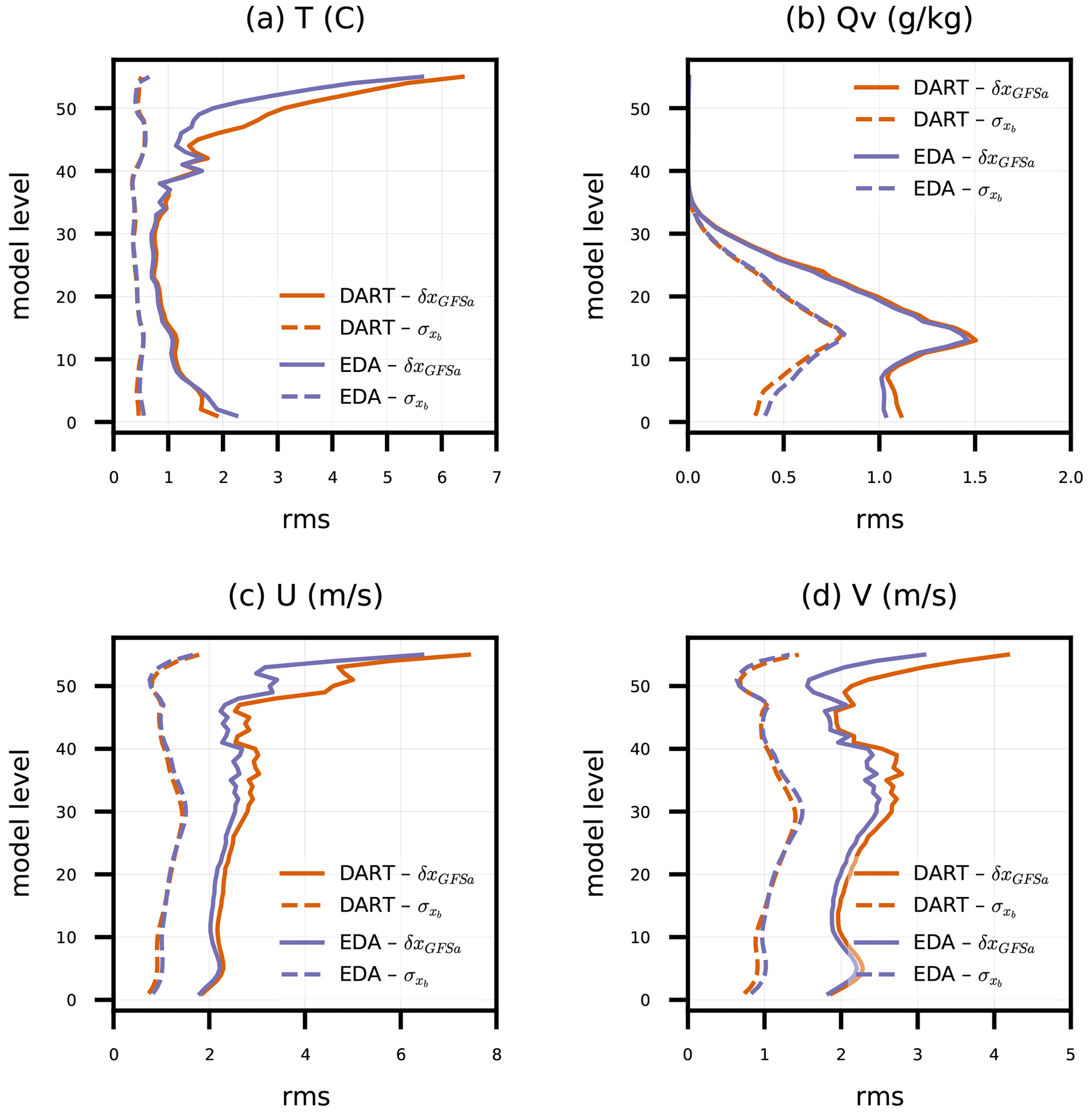
Figure 1Root mean square (rms) of ensemble-mean background difference to GFS analyses (δxGFSa) and background ensemble standard deviation () for model-simulated (a) temperature (T), (b) water vapor mixing ratio (Qv), and (c) zonal (U) and (d) meridional (V) wind components, all versus model level. Statistics are tabulated across all grid columns for DART and EDA experiments from every 6 h ensemble background between 00:00 UTC on 17 April 2018 and 00:00 UTC on 14 May 2018.
With those caveats in mind, Fig. 1 shows and rms(δxGFSa) for DART and EDA, aggregated over all horizontal columns and varying with model level. There is a strong indication that the background ensemble spreads are too small, or the RMSE is too large, especially near the top of the model and near the surface for T. Since we have not employed any measures to account for model uncertainty (see Sect. 2.1.2), we expect that the ensemble forecasts will be underdispersive. Overall, DART and EDA produce similar ensemble spreads and ensemble-mean RMSEs at most model levels.
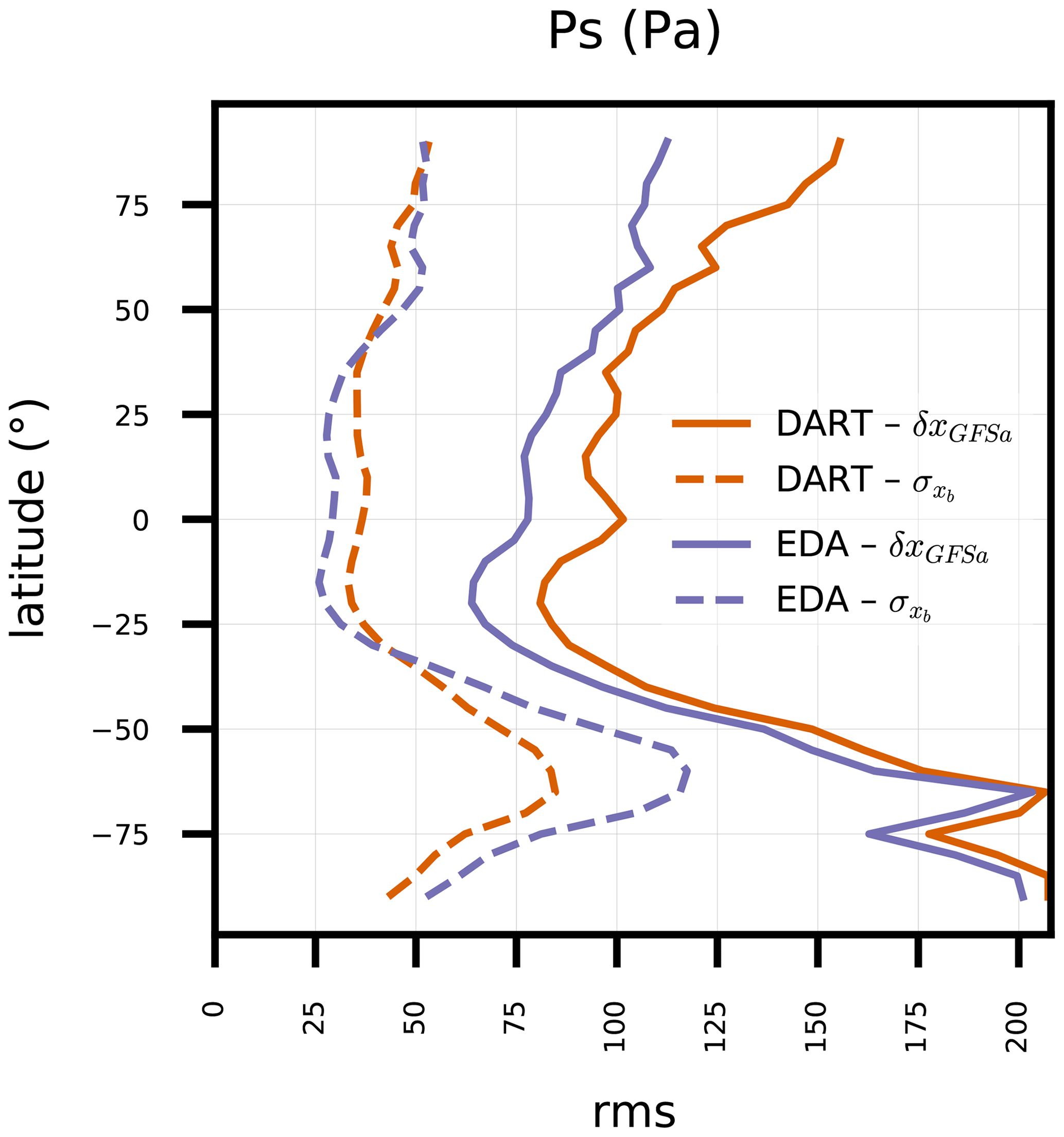
Figure 2 dissects the same quantities for model-simulated Ps, varying with latitude. There are obvious zonal differences between the two ensemble cycling experiments. DART produces slightly larger Ps spread than EDA in the tropics and smaller spread elsewhere. Those spread variations do not correlate directly with RMSE, since EDA produces a smaller RMSE at all latitudes. In separate diagnostics that further narrow down the Ps spread and RMSE on a world map (not shown), we found that DART's larger local spread correlates with lower RMSE in the western tropical Pacific Ocean, and EDA's smaller local spread correlates with lower RMSE in the tropical Atlantic Ocean and southeastern Pacific Ocean. Those correlations could be associated with the relative availabilities of local Ps observations, with there being slightly more available in the western Pacific.
The DART experiment has diminishing U and V ensemble spread in the tropical free troposphere as the cycling progresses (not shown). That spread loss could be caused by previously documented characteristics of RTPS, which Bowler et al. (2017b) found to produce inflation at much smaller scales than RTPP. Thus, that behavior is not indicative of relative performances of EAKF and EDA algorithms. The full investigation is reserved for future work, since the DART experiment is not the target of our current effort. However, the differences in U and V ensemble spread between DART and EDA have a non-negligible impact on the deterministic results presented in Sect. 5.2.
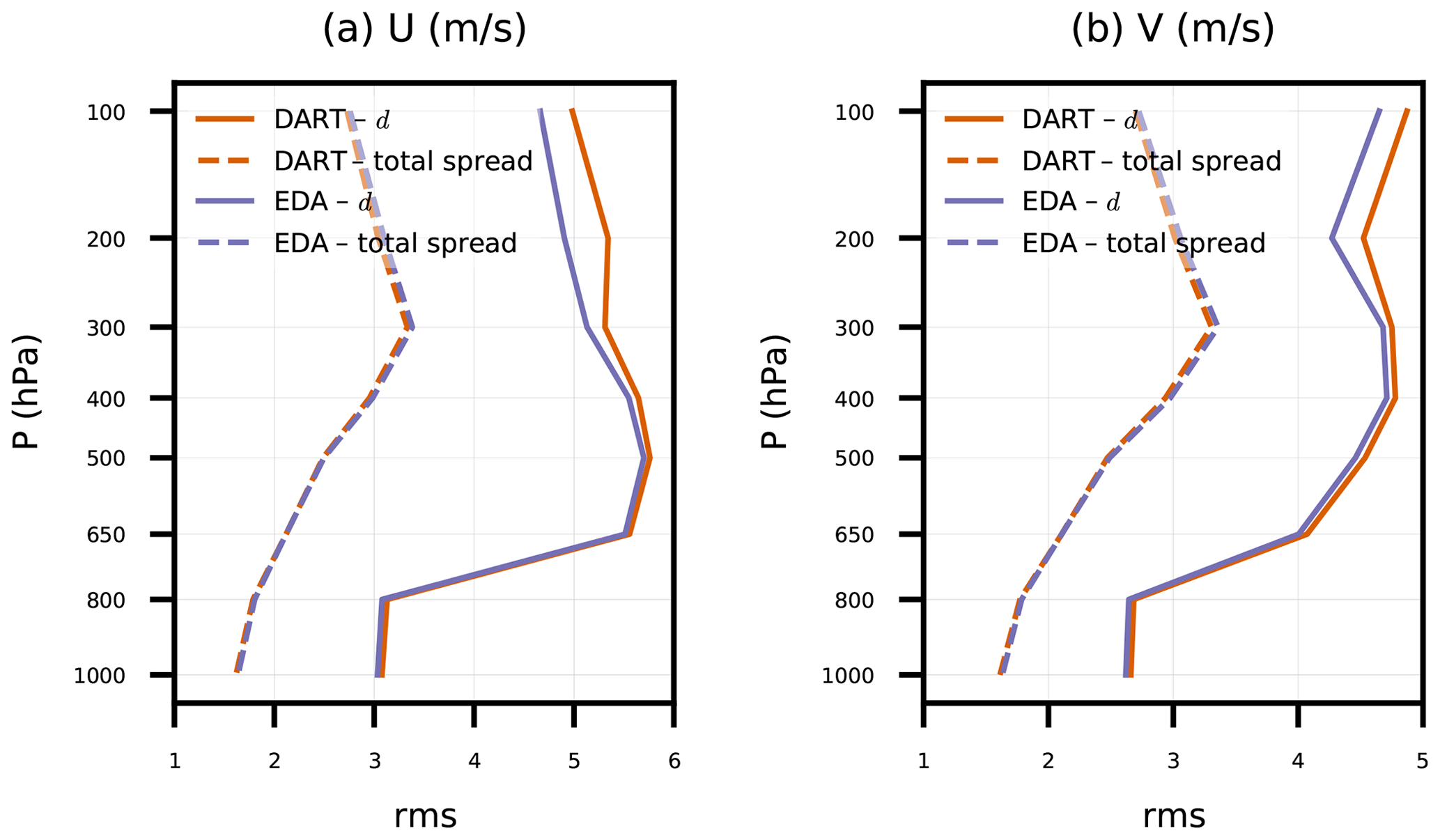
Figure 3Root mean square (rms) of ensemble-mean background innovation (d) and background ensemble total spread for satellite AMV (a) zonal and (b) meridional wind components versus pressure. Statistics are tabulated globally for DART and EDA experiments from every 6 h ensemble background between 00:00 UTC on 17 April 2018 and 00:00 UTC on 14 May 2018.
In fact, the ensemble spread decrease is likely the cause of differences in innovation RMSE for satellite AMVs between EDA and DART above 650 hPa (Fig. 3). Also shown are the total spread (Andersson et al., 2003; Desroziers et al., 2005) for both experiments. From Fig. 3, one might conclude that the observation error and/or the ensemble spread are too small to account for the ensemble-mean RMSE. After running all of the experiments in this study, we found that GSI assigns unique observation errors for each satellite AMV data source (e.g., Geostationary Operational Environmental Satellite, GOES; European Organisation for the Exploitation of Meteorological Satellites, EUMETSAT; Japan Meteorological Agency, JMA) and instrument band (e.g., infrared window, infrared water vapor, visible). Therefore the single vertical error distribution assigned in Table 1 for all AMVs needs to be revisited.
All things considered, the EDA and DART experiments produce remarkably similar behaviors. Those similarities are attributable to their commonalities in settings used for observation processing and lack of tuning. There are still many opportunities to reduce the prior ensemble-mean RMSE for both experiments, including observation error tuning, fixing known issues in GNSSRO assimilation (see Sect. 6), and assimilating more observation types. There are also many opportunities to increase the ensemble spread such that the consistency between spread and RMSE is improved, including accounting for model uncertainty, tuning the relaxation mechanism(s), and applying additive and prior inflation.
5.1 Setup
Both the EDA and DART ensemble cycling experiments successfully cycled for an entire month, independent of a higher-resolution centered EnVar state (i.e., such as that conducted by Liu et al., 2022). EDA and DART exhibit nearly stable spread characteristics, even if the spread tends to be too narrow relative to ensemble-mean RMSEs. Therefore, their respective background ensemble forecasts might be effective to use as Be in deterministic 3DEnVar cycling experiments. We conduct four deterministic dual-mesh 30 km–60 km 3DEnVar cycling experiments following the same approach as Liu et al. (2022), where the 30 km mesh is used in the DA outer loop and in forecasts, and the 60 km mesh is used for analysis increments in the DA inner loop. In the experiments presented, “dual-mesh” is wholly equivalent to a traditional dual-resolution incremental variational minimization. However, it is also possible to use variable-resolution meshes in either the inner or outer loop in JEDI-MPAS such that there may be many more than two mesh spacings (resolutions). EDA was limited to 1 outer iteration and 60 inner iterations for cost savings, but many more iterations are cheap in deterministic cycling. We apply 2 outer iterations, each with 60 inner iterations, to improve convergence toward observations with nonlinear operators. The same 1200 km horizontal and 6 km vertical localization length scales are applied as in the two ensemble experiments.
The only difference between the four deterministic experiments is the choice of BEC, which is summarized in Table 2. There are three pure 3DEnVar experiments – gefs100, dart100, and eda100 – that use 100 % ensemble BECs based on 20-member GEFS, 80-member DART, and 80-member EDA, respectively; gefs100 is equivalent to the clrama experiment from Liu et al. (2022).
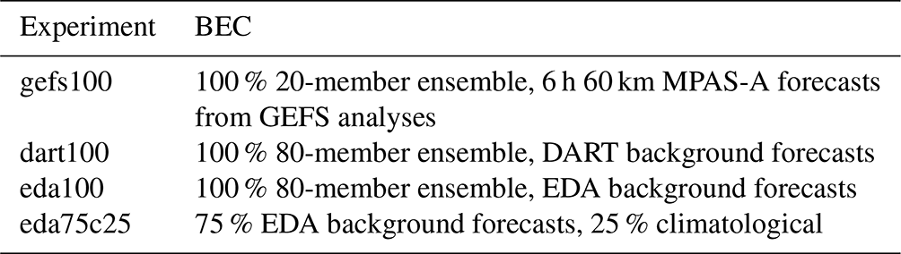
There is one hybrid 3DEnVar experiment, eda75c25, that uses a mixture of 75 % EDA ensemble and 25 % climatological BEC. The climatological BEC, Bc, is identical to the one described by Jung et al. (2023). Bc is trained using the National Meteorological Center (NMC) method (Parrish and Derber, 1992) with 366 samples of 48 h minus 24 h GFS forecast differences. The standard deviation of the trained Bc is scaled by , which was determined to be a quasi-optimal tuning justified by the need to match the 24 h forecast statistics to the 6 h background forecast duration. The horizontal length scales of stream function and unbalanced velocity potential (see Sect. 2.1 for more details) are scaled by to account for differences between the sampled correlation versus separation distance relationship and the Gaspari–Cohn fitting function used in BUMP. More details can be found in Jung et al. (2023).
All four experiments are initialized with a 6 h forecast initialized from a GFS analysis valid at 18:00 UTC on 14 April 2018, which was transformed to the MPAS-A 30 km mesh. The results that follow in Sect. 5.2 reflect statistics aggregated across twenty-seven 10 d forecasts initialized from 00:00 UTC analyses valid from 18 April 2018 to 14 May 2018. When error bars are shown, they indicate 95 % confidence intervals of those differences, tabulated via bootstrap resampling. Each of the binned RMSE differences from the 27 forecasts is treated as an independent and identically distributed sample, and they are resampled 10 000 times with replacement. The 95 % confidence intervals are then obtained by selecting the sample values at the 2.5th and 97.5th quantiles, referred to as the “percentile method” by Gilleland et al. (2018). It should be noted that the number of samples used here is small and does not account for seasonal variation in forecast quality. A more robust approach is needed when deploying an operational system.
5.2 Results
First we present results for the three pure 3DEnVar experiments to evaluate the efficacy of the EDA ensemble BEC. Our goal is to interrogate the EDA ensemble to determine its utility for future investigations and not to claim anything about its quality relative to the other data sources. A low water mark is for forecasts initialized from eda100 analyses to yield skills equivalent to or better than those initialized from gefs100 analyses; dart100 is included to demonstrate how small differences between EDA and DART affect deterministic cycling performance. As we describe in Sect. 4.2, those differences are not necessarily related to the ensemble DA algorithms.
Although GEFS was only available as a 20-member product during the period of experimentation presented herein, GEFS now provides 30-member ensemble forecasts (Zhou et al., 2022). In either case, the GEFS initial conditions are actually 6 h forecasts initialized from analyses drawn from the 80-member GDAS (Zhou et al., 2017). Therefore, they benefit from being produced by an 80-member EnKF. Additionally, GEFS initial conditions are expected to have added value over JEDI-MPAS's own ensemble because they benefit from the GDAS's EnKF assimilating many more observation types, having operational-quality observation error and inflation tuning, applying stochastic schemes to ensemble forecasts to treat model error, and being operated at a higher resolution.
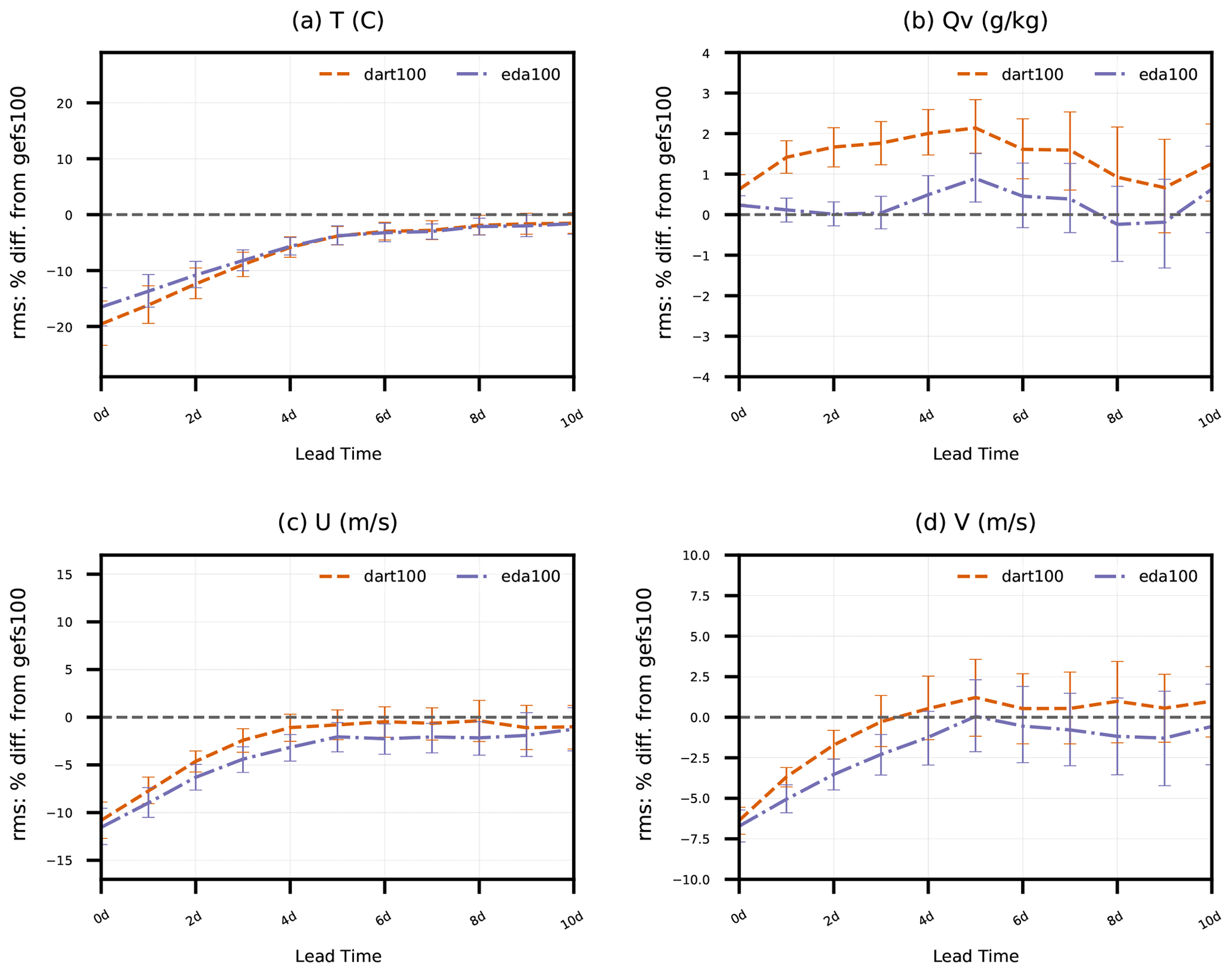
Figure 4Percent difference in rms(δxGFSa) of dart100 and eda100 with respect to rms(δxGFSa) of gefs100 (i.e., )). Values greater than zero indicate degradation relative to gefs100, while values less than zero indicate improvement. Error statistics are aggregated for all model grid columns and levels as a function of forecast lead time (0 to 10 d) for simulated (a) temperature, (b) specific humidity, and (c) zonal and (d) meridional wind components and pertain to 27 forecasts initialized from 00:00 UTC analyses from 18 April to 14 May 2018. Error bars indicate 95 % confidence intervals determined via bootstrap resampling (see text for description).
Figure 4 shows the dart100 and eda100 percent difference in RMSE with respect to GFS analyses compared to the RMSE of the control experiment, gefs100, in 0 to 10 d forecasts; eda100 performs better than gefs100 with 95 % confidence for T, U, and V. The relative performance of dart100 with respect to gefs100 follows similar trends for T, U, and V, slightly outperforming eda100 for T and slightly underperforming eda100 for U and V; eda100 produces a nearly neutral impact for Qv, although there is some degradation near the model top that dominates these vertically aggregated errors around day 5. The neutral Qv impact in this globally and vertically aggregated metric is likely due to the limited assimilation of moisture-sensitive observations (only sondes and aircraft). Assimilating radiances from water vapor channels in all-sky scenes (i.e., Liu et al., 2022) would better reveal the Qv impacts of these experimental ensembles.
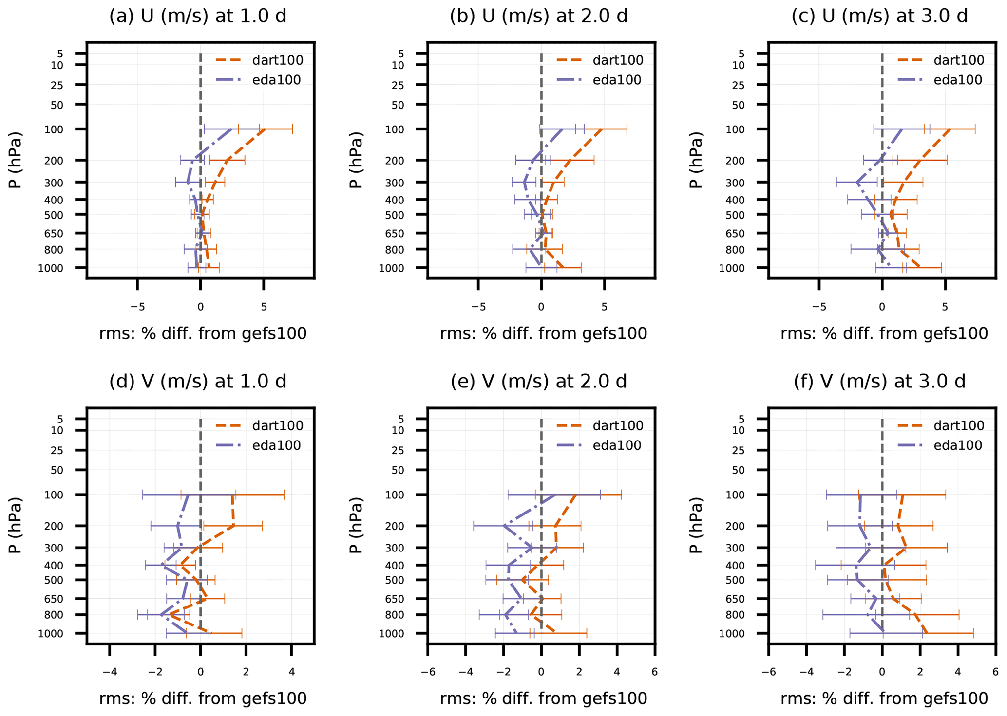
Figure 5Percent difference in rms(O-F) of dart100 and eda100 with respect to rms(O-F) of gefs100 for satellite AMVs. Error statistics are aggregated for individual pressure bins and as a function of forecast lead time (1 to 3 d) for (a–c) zonal and (d–f) meridional wind components and pertain to 27 forecasts initialized from 00:00 UTC from 18 April to 14 May 2018. Error bars indicate 95 % confidence intervals determined via bootstrap resampling (see text for description).
Figure 5 delves deeper into the largest source of wind observations to impact the DA analyses and subsequent forecasts: satellite AMVs. Although the verification against GFS analyses indicated improvement for both experiments, here the impact of the EDA ensemble in eda100 is nearly neutral for 1 to 3 d forecasts, and the DART ensemble has negative impacts, up to 5 % for U at 100 hPa, that are largely limited to tropical latitudes. As described in Sect. 4.2, the observation errors for satellite AMVs have much room for improvement, and the DART ensemble has decreasing transient U and V ensemble spread in the tropical free troposphere. More work remains to tune both the observation errors (e.g., following Desroziers et al., 2005) and BEC (either through spread tuning or covariance and localization improvements) in both the dart100 and eda100 experiments, which may explain some of the poor wind forecast quality.
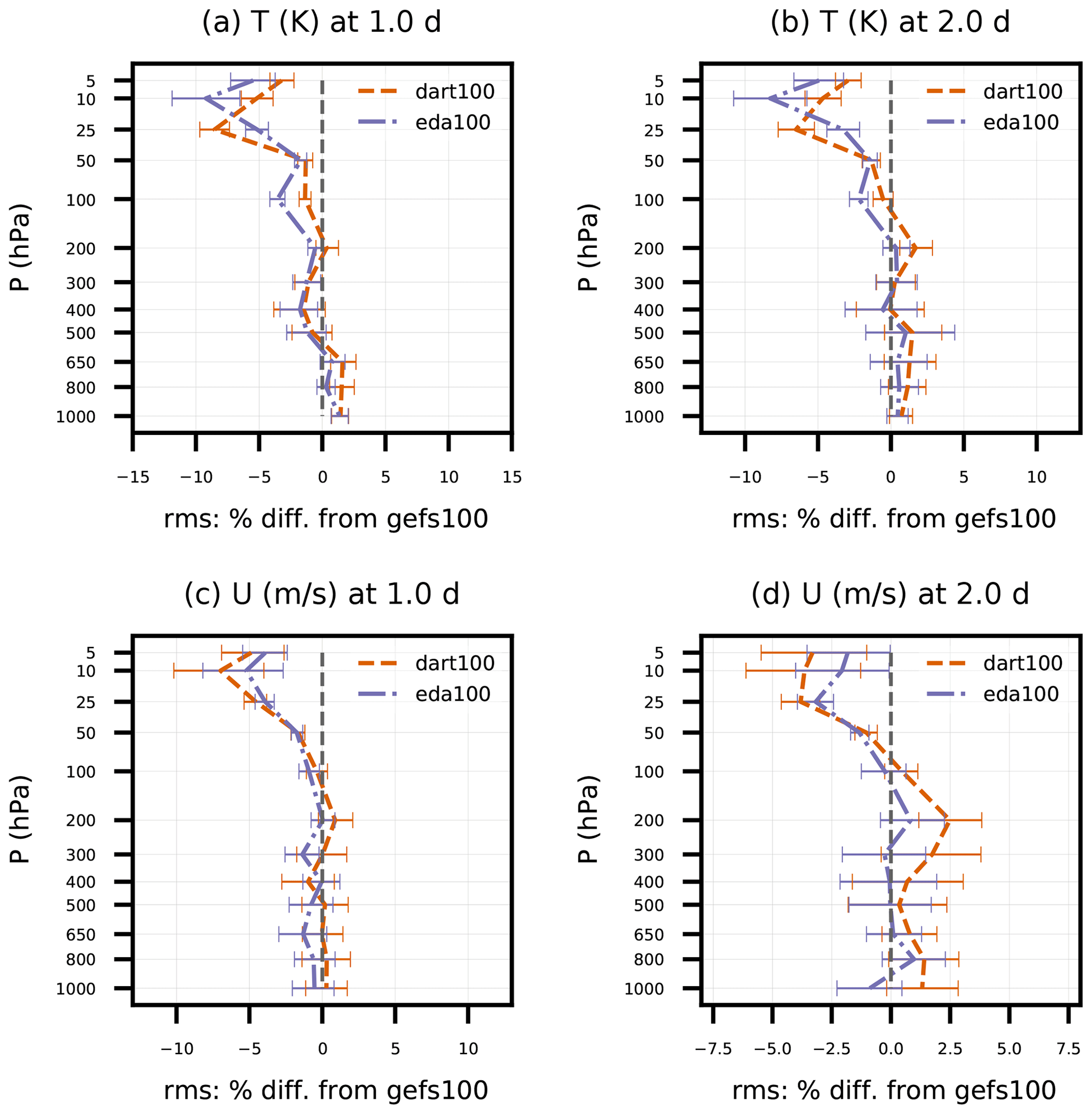
Figure 6Same as Fig. 5, except for 1 to 2 d forecasts of sonde (a–b) temperature and (c–d) zonal wind component between 30 and 90∘ N.
One observation that is generally consistent with the GFS analyses is sonde T and U in the Northern Hemisphere (Fig. 6). Both dart100 and eda100 achieve up to a 5 % positive impact above 50 hPa on day 1 for T and U, which slightly decreases on day 2. That positive T impact is collocated with a large cold bias that the non-GEFS BECs improve upon but do not remove entirely. Neither experiment gives statistically significant improvement in the troposphere compared to gefs100. Since the positive impact on sonde U is largely above 100 hPa, it is not surprising that is not reflected in the AMV verification, since satellite AMVs are located at 100 hPa and below.
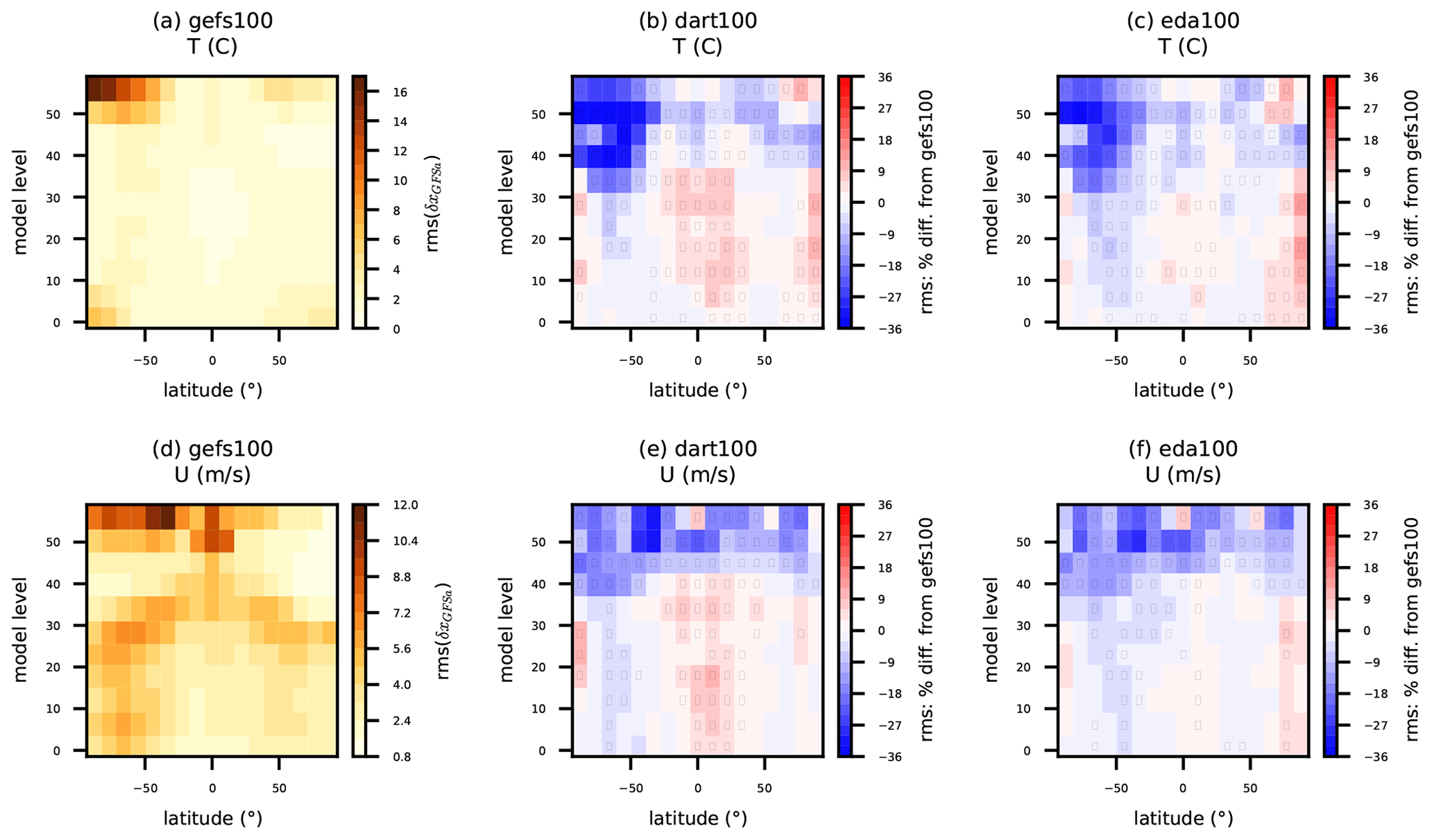
Figure 7(a, d) Reference rms(δxGFSa) for gefs100 and percent difference in rms(δxGFSa) for (b, e) dart100 and (c, f) eda100 at 2 d lead time. Statistics are binned in groups of ∼5 model levels and 11∘ latitude bands for simulated (a, b, c) temperature and (d, e, f) zonal wind component and pertain to 27 forecasts initialized from 00:00 UTC from 18 April to 14 May 2018. Inset black rectangles in individual bins indicate that the difference in rms between experiments is nonzero with at least 95 % confidence, as determined via bootstrap resampling (see text for description).
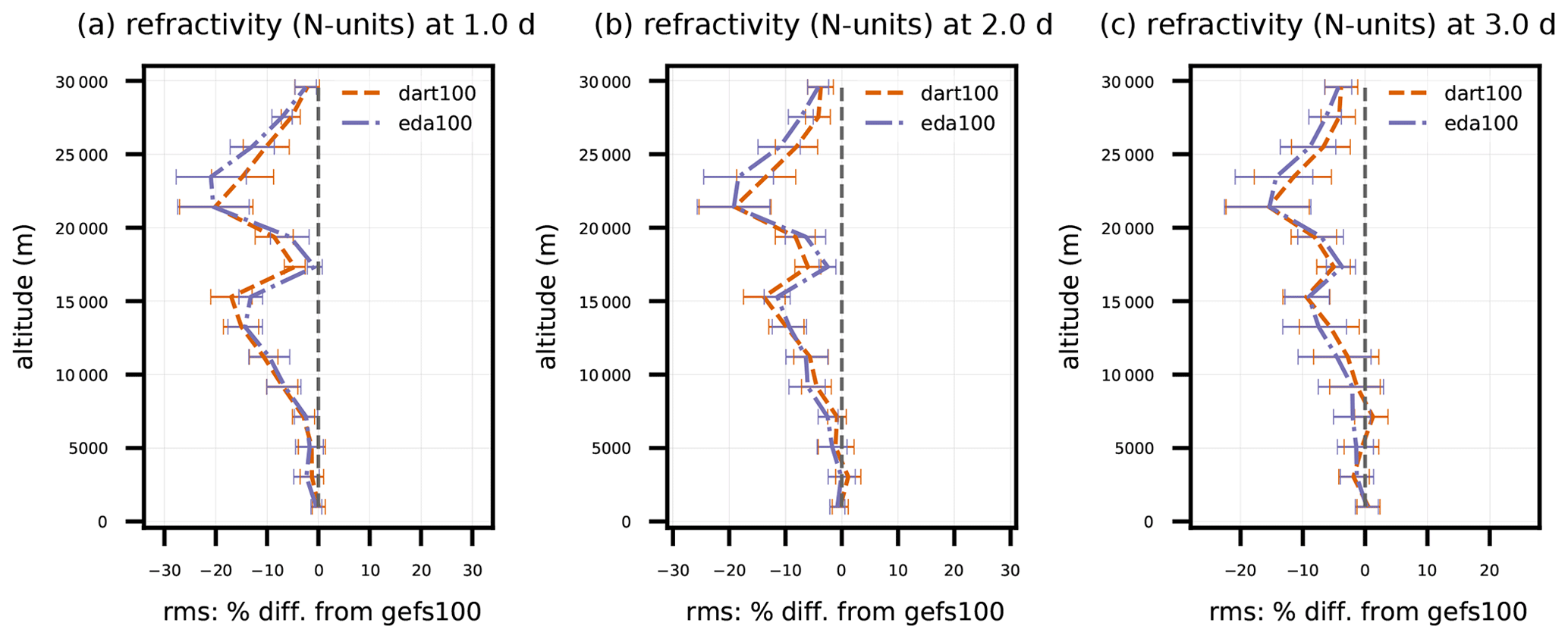
Figure 8Same as Fig. 5, except for GNSSRO refractivity versus altitude between 90 and 30∘ S. Error bars indicate 95 % confidence intervals determined via bootstrap resampling (see text for description).
That vertical distribution of T and U impacts is corroborated in model space via 2 d forecast verification versus GFS analyses (Fig. 7); dart100 and eda100 yield their largest improvements to T and U (more than 30 % locally) in the southern polar stratosphere (approximately above levels 35 to 40). Modest positive impacts are seen at most latitudes in the stratosphere consistently across both experiments. However, the tropical degradation in tropospheric T and U for dart100 is more obvious in this model-space verification. Also, eda100 has degradation in the northern polar troposphere. The vertical and latitudinal distribution of T impacts in dart100 and eda100 largely aligns with the impacts on GNSSRO refractivity.
Observations of GNSSRO refractivity, which is sensitive to T and Qv, indicate a positive tropospheric impact from both sets of 80-member BECs, although mostly limited to 40∘ S and poleward. Figure 8 shows the zonally aggregated dart100 and eda100 percent difference in RMSE with respect to refractivity compared to RMSE of gefs100 for 90 to 30∘ S. Both sensitivity experiments give a two-peak, statistically significant positive impact centered near 15 and 22 km altitudes, with a dip near the tropopause that might be explained by its misrepresentation in DA background states; eda100 and dart100 achieve at least a 15 % positive impact at some stratosphere altitudes out to day 3. In the troposphere, both experiments give comparable positive impacts, over 10 % on day 1 and declining slightly with lead time. All positive impacts in the Southern Hemisphere are above the planetary boundary layer. Although not shown in Fig. 8, the stratospheric impact of the 80-member BECs persists out to day 5.
It is useful to further explore the impacts of using a hybrid BEC because that algorithmic enhancement is readily adaptable to future EDA applications. Therefore, we first compare eda75c25 to eda100 to demonstrate the benefits of additionally accounting for climatological BECs and then to gefs100 to show the total impact of developments herein and in Jung et al. (2023).
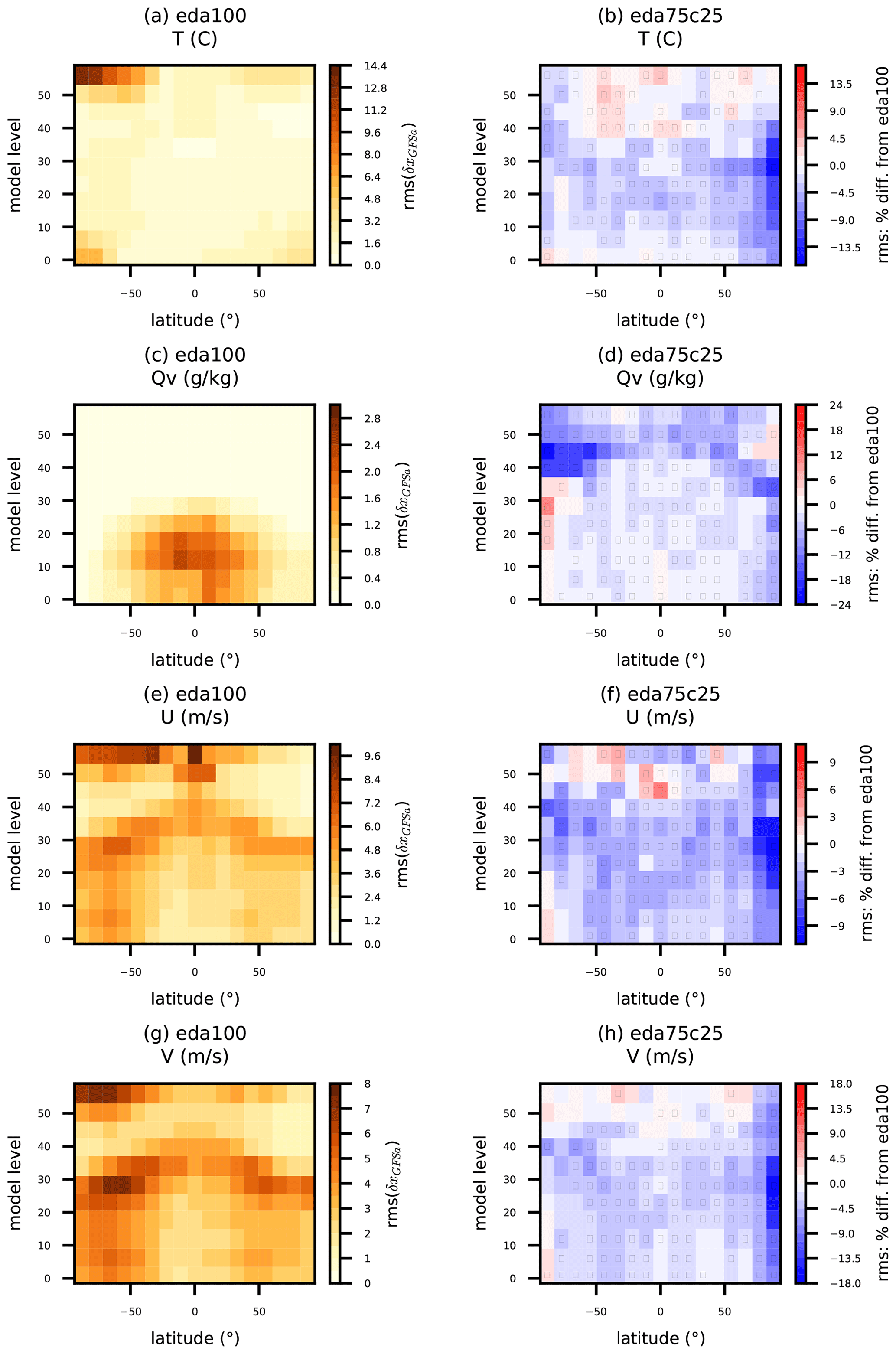
Figure 9Same as Fig. 7, except that the (a, c, e, g) reference rms is for eda100, and (b, d, f, h) percent difference is shown for eda75c25. Statistics are tabulated for simulated (a, b) temperature, (c, d) water vapor mixing ratio, and (e, f) zonal and (g, h) meridional wind components.
Adding the 25 % climatological BEC component and scaling the 80-member ensemble BEC component by 75 % adds significant value across a wide range of observation- and model-space verification metrics. Figure 9 shows the T, Qv, U, and V RMSE with respect to GFS analyses at 2 d lead time for eda100 and the corresponding percent differences in RMSE for eda75c25. Most of the positive impacts for T are limited to the troposphere (below model levels 35–40) and reach up to 14 % above the North Pole. Since the EDA ensemble caused some degradation near the North Pole and did not cause much improvement outside the southern extratropical to polar free troposphere and stratosphere, this is a welcome benefit. The eda75c25 2 d forecast moisture also aligns better with GFS analyses than eda100, although this also makes up for some degradation in stratospheric Qv between eda100 and gefs100. Overall, eda75c25 consistently improves the 2 d wind forecasts throughout the troposphere. It is clear that the climatological BEC makes up for information that is lacking in the completely flow-dependent ensemble BEC.
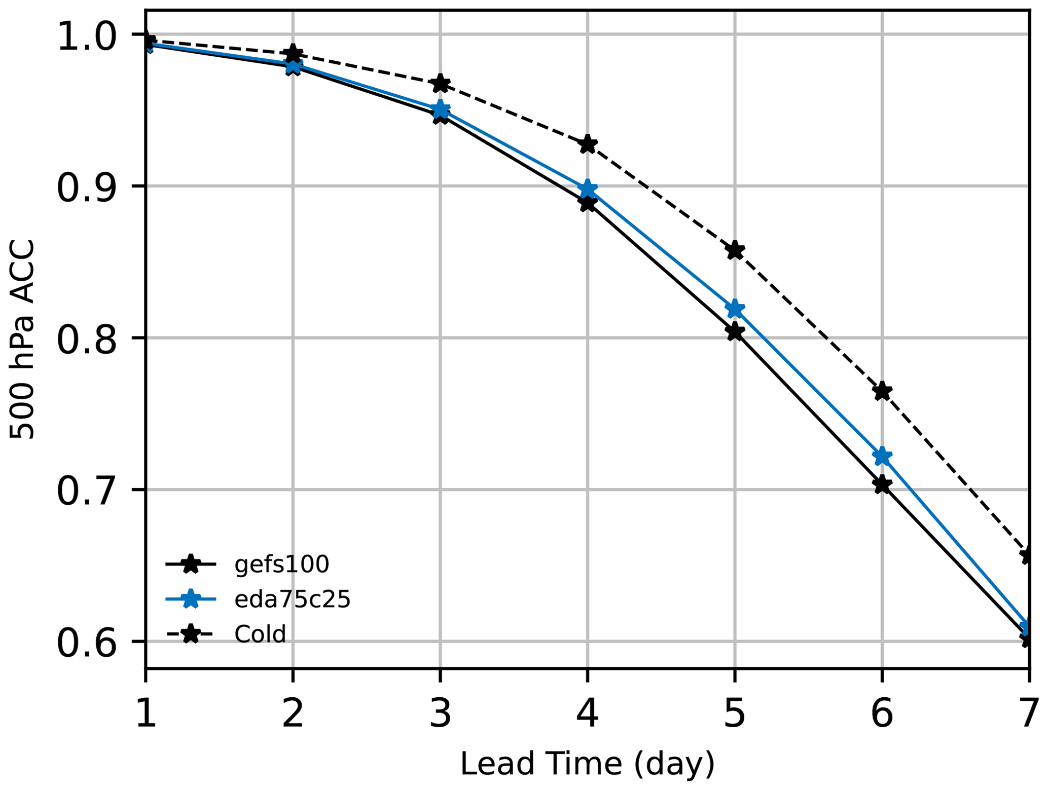
Figure 10The 1 to 7 d anomaly correlation coefficient (ACC) of 500 hPa geopotential height for gefs100, eda75c25, and cold-start forecasts initialized from GFS analyses (Cold). Statistics are tabulated over all grid cells and pertain to 17 forecasts initialized from 00:00 UTC from 18 April to 4 May 2018.
Finally, we consider a metric which incorporates information from multiple variables. According to Krishnamurti et al. (2003), a 500 hPa geopotential height anomaly correlation coefficient (ACC) “greater than 0.6 generally implies that troughs and ridges at 500 hPa are beginning to be properly placed in that forecast.” We calculate anomalies with respect to the climatology derived from the 1980–2010 NCEP/NCAR reanalysis products (Kalnay et al., 1996). We conduct cold-start forecasts initialized from GFS analyses as a reference. The cold-start forecast anomalies are compared to those of GFS analyses. For the eda75c25 and gefs100 experiments, their forecast anomalies are compared to those of their respective analyses. Figure 10 shows the 1 to 7 d forecast ACC scores for eda75c25, gefs100, and the cold-start forecasts. The gefs100 forecasts are approximately 0.6 d behind the GFS analyses at ; eda75c25 provides approximately 0.1 to 0.2 d enhanced predictability for 4 to 6 d forecasts globally.
The EDA ensemble-based BEC and the climatological BEC contribute complementary information in the deterministic cycling. Although there are still many avenues for future improvements, these BECs are ready for the non-developer user base. On the basis of this work, JEDI-MPAS has the means to produce an ensemble of forecasts without relying on an external analysis system at each cycle.
This paper documents the implementation of En-3DEnVar for JEDI-MPAS, and demonstrates its use in both ensemble cycling and experiments in which a previously computed EDA ensemble provides the BEC for cycling EnVar.
Our cycling DA experiments previously required ensembles of initial conditions from an external system (GEFS) (Liu et al., 2022). Using EDA gives ensemble initial conditions that are consistent with the configuration of MPAS (for example, including a set of hydrometeors consistent with the chosen microphysical scheme) and with the observing network used. The EDA also performs better in most scores relative to our previous approach, though with increased computational cost. As a further check on the implementation of EDA, we compared against an experiment using MPAS-DART, a more mature ensemble data assimilation system, for ensemble BEC generation and found comparable performance in terms of ensemble spread, ensemble-mean background RMSE, and subsequent deterministic cycling forecast quality. A further refinement, which improves relative to using the EDA in EnVar alone and across almost all latitudes and heights, is the use of a hybrid BEC that is a weighted sum of the ensemble covariances and the static covariances of Jung et al. (2023). With this refinement, the system is ready to produce research-quality ensembles for future sensitivity studies that aim to enhance JEDI-MPAS.
A non-standard element of our experiments is the use of self-exclusion, as in Bowler et al. (2017a) and Buehner (2020). In the update for a given member, the ensemble covariance in the BEC is based on the remaining members, with its own member “excluded”. Self-exclusion improves the EDA results because it significantly reduces the EDA bias toward underestimating the analysis spread. We defer further analysis of self-exclusion to a separate paper.
The largest improvements from EDA relative to using GEFS-based BEC are found in temperature and wind in the stratosphere and throughout the Southern Hemisphere. The improvements in the stratosphere come despite the EDA ensemble being underdispersive there and despite substantial stratospheric temperature biases in both the analyses and forecasts. We have since conducted multiple sensitivity tests where we assimilate GNSSRO bending angle instead of refractivity and carefully tune the bending angle observation errors. Those experiments reduce the stratospheric temperature bias significantly, and additional corrective measures are still under investigation.
There are several paths to further improvements in the short-range ensemble forecasts produced by the JEDI-MPAS En-3DEnVar. In all ensemble and deterministic experiments, most of the settings for observation error (R) and QC are taken directly from operational-center-specific implementations in either UFO or GSI, and they reflect the characteristic behavior of a different cycling system. Now that full deterministic and ensemble cycling functionality has been demonstrated with JEDI-MPAS, those settings can be robustly analyzed and tuned (e.g., Desroziers et al., 2005). Accounting for model error in the ensemble-forecast step is also a top priority. Finally, additional improvements could be achieved in EDA by using at least two outer iterations with more total inner iterations or by enabling an En-4DEnVar, both with corresponding increases in cost.
Previous studies (e.g., Lorenc et al., 2017; Buehner et al., 2017) have pointed out the significantly greater computational expense of EDA based on EnVar compared to an EnKF. The same is true here: the EDA algorithm was roughly 4 times more expensive than the DART EAKF algorithm, both with 80 members. The primary drivers of EDA cost are the (1) reading and storing of 80 ensemble background states by each of those independent Variational members and (2) the performance of localization and multiplication for the 80 perturbations in each inner-loop iteration; together those account for of the total cost of the DA step. While recent model-space localization techniques hold promise for maintaining analysis covariance quality with fewer EDA members (i.e., Lorenc, 2017), we did not exercise those here. However, the total number of members strongly impacts both the EnKF and EDA costs.
A solution to problem 1 using parallelization strategies across minimization members was proposed by Arbogast et al. (2017). A number of techniques also exist to address problem 2. The multi-mesh minimizations used in deterministic experiments in Sect. 5 can be extended to the EDA. “Mean–pert” methods (Lorenc et al., 2017; Buehner et al., 2017) reduce computational costs by simplifying the update of ensemble perturbations as compared to that of the ensemble mean. Bowler et al. (2017b) used a mean–pert algorithm to realize a cost reduction of a factor of 3 in their En-4DEnVar (Lorenc et al., 2017). Block EDA algorithms (Mercier et al., 2018) also hold promise for reducing inner iteration count, which Gas (2021) demonstrated in JEDI. Finally, because JEDI is relatively immature, there also remain many opportunities for basic computational optimization of JEDI-MPAS. For example, after completing the EDA and DART experiments, a single-precision in-core memory and computation capability was added for JEDI-MPAS states (e.g., xb, xa) and increments (e.g., δx). This development reduces the cost for the DA step of the EDA experiment by 25 %
The progress demonstrated herein is a testament to the fact that innovations introduced into JEDI by one contributor (e.g., JCSDA, NOAA, NASA, US Navy, US Air Force, UK Met Office, NCAR) are more easily leveraged by partners than was previously possible with separate DA software frameworks. Together with Liu et al. (2022) and Jung et al. (2023), the demonstration of EDA for JEDI-MPAS provides a foundation for more complex endeavors. In particular, variable mesh resolution is one of the main motivations for MPAS-A and has been demonstrated to produce more realistic forecasts than a nested domain near regions of mesh refinement (Park et al., 2014). Work is already under way to demonstrate variable-resolution and regional mesh capabilities in JEDI-MPAS.
JEDI-MPAS 2.0.0-beta is publicly released on GitHub and accessible in the release/2.0.0-beta branch of mpas-bundle (https://github.com/JCSDA/mpas-bundle/tree/release/2.0.0-beta, last access: 8 March 2023). It is also available from Zenodo at https://doi.org/10.5281/zenodo.7630054 (Joint Center For Satellite Data Assimilation and National Center For Atmospheric Research, 2022). Global Forecast System analysis data are downloaded from the NCAR Research Data Archive https://doi.org/10.5065/D65D8PWK (National Centers for Environmental Prediction/National Weather Service/NOAA/U.S. Department of Commerce, 2015). Global Ensemble Forecast System ensemble analysis data are downloaded from https://www.ncei.noaa.gov/products/weather-climate-models/global-ensemble-forecast (last access: 21 October 2022). Conventional and satellite observations assimilated are downloaded from https://doi.org/10.5065/Z83F-N512 (National Centers for Environmental Prediction/National Weather Service/NOAA/U.S. Department of Commerce, 2008), https://doi.org/10.5065/DWYZ-Q852 (National Centers for Environmental Prediction/National Weather Service/NOAA/U.S. Department of Commerce, 2009), and https://doi.org/10.5065/39C5-Z211 (Satellite Services Division, 2004).
The first author designed, conducted, and analyzed all En-3DEnVar and 3DEnVar experiments and wrote the manuscript. ZL and CS aided with experiment design and analysis. CSS designed and conducted the DART cycling experiment and wrote the description for MPAS-DART and the associated experiment. All co-authors contributed to the development of the JEDI-MPAS source code and experimental workflow, preparation of externally sourced data, design of experiments, and preparation of the manuscript.
The contact author has declared that none of the authors has any competing interests.
Publisher’s note: Copernicus Publications remains neutral with regard to jurisdictional claims made in the text, published maps, institutional affiliations, or any other geographical representation in this paper. While Copernicus Publications makes every effort to include appropriate place names, the final responsibility lies with the authors.
The National Center for Atmospheric Research is sponsored by the National Science Foundation of the United States. We would like to acknowledge high-performance computing support from Cheyenne (https://doi.org/10.5065/D6RX99HX, Computational and Information Systems Laboratory, 2019) provided by NCAR's Computational and Information Systems Laboratory, sponsored by the National Science Foundation. Michael Duda in the Mesoscale and Microscale Meteorology (MMM) laboratory provided guidance on modifying MPAS-A for JEDI-MPAS applications. We are thankful to the two anonymous reviewers and to Lili Lei for their insightful suggestions on improving the final paper.
This research has been supported by the US Air Force (grant no. NA21OAR4310383).
This paper was edited by Shu-Chih Yang and reviewed by two anonymous referees.
Anderson, J., Hoar, T., Raeder, K., Liu, H., Collins, N., Torn, R., and Avellano, A.: The Data Assimilation Research Testbed: A Community Facility, B. Am. Meteor. Soc., 90, 1283–1296, https://doi.org/10.1175/2009bams2618.1, 2009. a, b
Anderson, J. L.: An Ensemble Adjustment Kalman Filter for Data Assimilation, Mon. Weather Rev., 129, 2884–2903, https://doi.org/10.1175/1520-0493(2001)129<2884:aeakff>2.0.co;2, 2001. a, b
Anderson, J. L.: A Local Least Squares Framework for Ensemble Filtering, Mon. Weather Rev., 131, 634–642, https://doi.org/10.1175/1520-0493(2003)131<0634:allsff>2.0.co;2, 2003. a
Anderson, J. L.: A Non-Gaussian Ensemble Filter Update for Data Assimilation, Mon. Weather Rev., 138, 4186–4198, https://doi.org/10.1175/2010mwr3253.1, 2010. a
Anderson, J. L.: A Marginal Adjustment Rank Histogram Filter for Non-Gaussian Ensemble Data Assimilation, Mon. Weather Rev., 148, 3361–3378, https://doi.org/10.1175/mwr-d-19-0307.1, 2020. a
Anderson, J. L. and Collins, N.: Scalable Implementations of Ensemble Filter Algorithms for Data Assimilation, J. Atmos. Ocean. Tech., 24, 1452–1463, https://doi.org/10.1175/jtech2049.1, 2007. a
Andersson, E., Bouttier, F., Cardinali, C., Isaksen, L., and Saarinen, S.: Modelling of innovation statistics, in: Workshop on recent developments in data assimilation for atmosphere and ocean, ECMWF Annual Seminar 2003, ECMWF, Reading, UK, 8–12 September 2003, https://www.ecmwf.int/en/elibrary/15973-modelling-innovation-statistics (last access: 30 November 2022), 2003. a
Arbogast, É., Desroziers, G., and Berre, L.: A parallel implementation of a 4DEnVar ensemble, Q. J. Roy. Meteor. Soc., 143, 2073–2083, https://doi.org/10.1002/qj.3061, 2017. a, b
Berre, L. and Desroziers, G.: Filtering of Background Error Variances and Correlations by Local Spatial Averaging: A Review, Mon. Weather Rev., 138, 3693–3720, https://doi.org/10.1175/2010mwr3111.1, 2010. a
Berre, L., Ştefănescu, S. E., and Pereira, M. B.: The representation of the analysis effect in three error simulation techniques, Tellus A, 58, 196, https://doi.org/10.1111/j.1600-0870.2006.00165.x, 2006. a
Berre, L., Pannekoucke, O., Desroziers, G., Stefanescu, S. E., Chapnik, B., and Raynaud, L.: A variational assimilation ensemble and the spatial filtering of its error covariances: increase of sample size by local spatial averaging, in: Workshop on Flow-dependent aspects of data assimilation, 11–13 June 2007, ECMWF, Shinfield Park, Reading, https://www.ecmwf.int/en/elibrary/8172-variational-assimilation-ensemble-and-spatial-filtering-its-error-covariances (last access: 28 October 2022), 2007. a
Bishop, C. H., Whitaker, J. S., and Lei, L.: Gain Form of the Ensemble Transform Kalman Filter and Its Relevance to Satellite Data Assimilation with Model Space Ensemble Covariance Localization, Mon. Weather Rev., 145, 4575–4592, https://doi.org/10.1175/mwr-d-17-0102.1, 2017. a
Bonavita, M., Hamrud, M., and Isaksen, L.: EnKF and Hybrid Gain Ensemble Data Assimilation. Part II: EnKF and Hybrid Gain Results, Mon. Weather Rev., 143, 4865–4882, https://doi.org/10.1175/mwr-d-15-0071.1, 2015. a
Bowler, N. E., Flowerdew, J., and Pring, S. R.: Tests of different flavours of EnKF on a simple model, Q. J. Roy. Meteor. Soc., 139, 1505–1519, https://doi.org/10.1002/qj.2055, 2012. a
Bowler, N. E., Clayton, A. M., Jardak, M., Jermey, P. M., Lorenc, A. C., Wlasak, M. A., Barker, D. M., Inverarity, G. W., and Swinbank, R.: The effect of improved ensemble covariances on hybrid variational data assimilation, Q. J. Roy. Meteor. Soc., 143, 785–797, https://doi.org/10.1002/qj.2964, 2017a. a, b, c
Bowler, N. E., Clayton, A. M., Jardak, M., Lee, E., Lorenc, A. C., Piccolo, C., Pring, S. R., Wlasak, M. A., Barker, D. M., Inverarity, G. W., and Swinbank, R.: Inflation and localization tests in the development of an ensemble of 4D-ensemble variational assimilations, Q. J. Roy. Meteor. Soc., 143, 1280–1302, https://doi.org/10.1002/qj.3004, 2017b. a, b, c, d, e, f, g, h, i, j
Buehner, M.: Ensemble-derived stationary and flow-dependent background-error covariances: Evaluation in a quasi-operational NWP setting, Q. J. Roy. Meteor. Soc., 131, 1013–1043, https://doi.org/10.1256/qj.04.15, 2005. a
Buehner, M.: Local Ensemble Transform Kalman Filter with Cross Validation, Mon. Weather Rev., 148, 2265–2282, https://doi.org/10.1175/mwr-d-19-0402.1, 2020. a, b, c
Buehner, M., McTaggart-Cowan, R., and Heilliette, S.: An ensemble Kalman filter for numerical weather prediction based on variational data assimilation: VarEnKF, Mon. Weather Rev., 145, 617–635, https://doi.org/10.1175/MWR-D-16-0106.1, 2017. a, b, c
Burgers, G., van Leeuwen, P. J., and Evensen, G.: Analysis Scheme in the Ensemble Kalman Filter, Mon. Weather Rev., 126, 1719–1724, https://doi.org/10.1175/1520-0493(1998)126<1719:asitek>2.0.co;2, 1998. a
Campbell, W. F., Bishop, C. H., and Hodyss, D.: Vertical Covariance Localization for Satellite Radiances in Ensemble Kalman Filters, Mon. Weather Rev., 138, 282–290, https://doi.org/10.1175/2009mwr3017.1, 2010. a
Computational and Information Systems Laboratory: Cheyenne: HPE/SGI ICE XA System (NCAR Community Computing), Boulder, CO: National Center for Atmospheric Research, https://doi.org/10.5065/D6RX99HX, 2019. a
Derber, J. and Bouttier, F.: A reformulation of the background error covariance in the ECMWF global data assimilation system, Tellus A, 51, 195–221, https://doi.org/10.3402/tellusa.v51i2.12316, 1999. a
Desroziers, G., Berre, L., Chapnik, B., and Poli, P.: Diagnosis of observation, background and analysis-error statistics in observation space, Q. J. Roy. Meteor. Soc., 131, 3385–3396, https://doi.org/10.1256/qj.05.108, 2005. a, b, c
Desroziers, G., Berre, L., and Pannekoucke, O.: Flow-dependent error covariances from variational assimilation ensembles on global and regional domains, Météo-France, Toulouse, France, HIRLAM Technical Report No. 68, https://www.umr-cnrm.fr/recyf/IMG/pdf/HIRLAM_TR68_Paper1_Desroziers.pdf (last access: 28 October 2022), 2008. a
Evensen, G.: The Ensemble Kalman Filter: theoretical formulation and practical implementation, Ocean Dynam., 53, 343–367, https://doi.org/10.1007/s10236-003-0036-9, 2003. a
Fisher, M.: Background Error Covariance Modeling, in: Seminar on Recent developments in data assimilation for atmosphere and ocean, ECMWF, Shinfield Park, Reading, 8–12 September 2003, https://www.ecmwf.int/en/elibrary/9404-background-error-covariance-modelling (last access: 28 October 2022), 2003. a
Gas, C.: Block Method Minimizer for Solving Ensemble of Data Assimilation, 18th JCSDA Technical Review Meeting and Science Workshop, Held Virtually, 7–11 June 2021, http://data.jcsda.org/Workshops/JCSDA-18th-Workshop/Tuesday/8.Gas.pdf (last access: 28 October 2022), 2021. a
Gilleland, E., Hering, A. S., Fowler, T. L., and Brown, B. G.: Testing the Tests: What Are the Impacts of Incorrect Assumptions When Applying Confidence Intervals or Hypothesis Tests to Compare Competing Forecasts?, Mon. Weather Rev., 146, 1685–1703, https://doi.org/10.1175/mwr-d-17-0295.1, 2018. a
Greybush, S. J., Kalnay, E., Miyoshi, T., Ide, K., and Hunt, B. R.: Balance and Ensemble Kalman Filter Localization Techniques, Mon. Weather Rev., 139, 511–522, https://doi.org/10.1175/2010mwr3328.1, 2011. a
Ha, S., Snyder, C., Skamarock, W. C., Anderson, J., and Collins, N.: Ensemble Kalman Filter Data Assimilation for the Model for Prediction Across Scales (MPAS), Mon. Weather Rev., 145, 4673–4692, https://doi.org/10.1175/mwr-d-17-0145.1, 2017. a, b
Hamill, T. M., Snyder, C., and Morss, R. E.: A comparison of probabilistic forecasts from bred, singular-vector, and perturbed observation ensembles, Mon. Weather Rev., 128, 1835–1851, https://doi.org/10.1175/1520-0493(2000)128<1835:ACOPFF>2.0.CO;2, 2000. a
Hamrud, M., Bonavita, M., and Isaksen, L.: EnKF and Hybrid Gain Ensemble Data Assimilation. Part I: EnKF Implementation, Mon. Weather Rev., 143, 4847–4864, https://doi.org/10.1175/mwr-d-14-00333.1, 2015. a
Honeyager, R., Herbener, S., Zhang, X., Shlyaeva, A., and Trémolet, Y.: Observations in the Joint Effort for Data Assimilation Integration (JEDI) – Unified Forward Operator (UFO) and Interface for Observation Data Access (IODA), JCSDA Quarterly Newsletter, 66, 24–34, https://doi.org/10.25923/RB19-0Q26, 2020. a, b
Houtekamer, P. L. and Derome, J.: Methods for ensemble prediction, Mon. Weather Rev., 123, 2181–2196, https://doi.org/10.1175/1520-0493(1995)123<2181:MFEP>2.0.CO;2, 1995. a
Houtekamer, P. L. and Mitchell, H. L.: Data Assimilation Using an Ensemble Kalman Filter Technique, Mon. Weather Rev., 126, 796–811, https://doi.org/10.1175/1520-0493(1998)126<0796:dauaek>2.0.co;2, 1998. a, b
Houtekamer, P. L., Lefaivre, L., Derome, J., Ritchie, H., and Mitchell, H. L.: A system simulation approach to ensemble prediction, Mon. Weather Rev., 124, 1225–1242, https://doi.org/10.1175/1520-0493(1996)124<1225:ASSATE>2.0.CO;2, 1996. a
Ingleby, B.: Global assimilation of air temperature, humidity, wind and pressure from surface stations: practice and performance, Met Office, Exeter, UK, Forecasting Research Technical Report 582, https://digital.nmla.metoffice.gov.uk/digitalFile_e12ba2af-84e9-45f2-8f30-146ae421f45c/ (last access: 28 October 2022), 2013. a
Isaksen, L., Bonavita, M., Buizza, R., Fisher, M., Haseler, J., Leutbecher, M., and Raynaud, L.: Ensemble of data assimilations at ECMWF, Technical Memoranda 636, https://doi.org/10.21957/OBKE4K60, 2010. a
Joint Center For Satellite Data Assimilation and National Center For Atmospheric Research: JEDI-MPAS Data Assimilation System v2.0.0-beta, Zenodo [code], https://doi.org/10.5281/zenodo.7630054, 2022. a
Jung, B.-J., Ménétrier, B., Snyder, C., Liu, Z., Guerrette, J. J., Ban, J., Baños, I. H., Yu, Y. G., and Skamarock, W. C.: Three-dimensional variational assimilation with a multivariate background error covariance for the Model for Prediction Across Scales–Atmosphere with the Joint Effort for data Assimilation Integration (JEDI-MPAS 2.0.0-beta), Geosci. Model Dev. Discuss. [preprint], https://doi.org/10.5194/gmd-2023-131, in review, 2023. a, b, c, d, e, f
Kalnay, E., Kanamitsu, M., Kistler, R., Collins, W., Deaven, D., Gandin, L., Iredell, M., Saha, S., White, G., Woollen, J., Zhu, Y., Leetmaa, A., Reynolds, R., Chelliah, M., Ebisuzaki, W., Higgins, W., Janowiak, J., Mo, K. C., Ropelewski, C., Wang, J., Jenne, R., and Joseph, D.: The NCEP/NCAR 40-Year Reanalysis Project, B. Am. Meteor. Soc., 77, 437–471, https://doi.org/10.1175/1520-0477(1996)077<0437:TNYRP>2.0.CO;2, 1996. a
Kleist, D. T. and Ide, K.: An OSSE-Based Evaluation of Hybrid Variational–Ensemble Data Assimilation for the NCEP GFS. Part II: 4DEnVar and Hybrid Variants, Mon. Weather Rev., 143, 452–470, https://doi.org/10.1175/mwr-d-13-00350.1, 2015. a
Kotsuki, S., Ota, Y., and Miyoshi, T.: Adaptive covariance relaxation methods for ensemble data assimilation: experiments in the real atmosphere, Q. J. Roy. Meteor. Soc., 143, 2001–2015, https://doi.org/10.1002/qj.3060, 2017. a
Krishnamurti, T. N., Rajendran, K., Kumar, T. S. V. V., Lord, S., Toth, Z., Zou, X., Cocke, S., Ahlquist, J. E., and Navon, I. M.: Improved Skill for the Anomaly Correlation of Geopotential Heights at 500 hPa, Mon. Weather Rev., 131, 1082–1102, https://doi.org/10.1175/1520-0493(2003)131<1082:isftac>2.0.co;2, 2003. a
Lawless, A. S., Gratton, S., and Nichols, N. K.: Approximate iterative methods for variational data assimilation, Int. J. Numer. Meth. Fl., 47, 1129–1135, https://doi.org/10.1002/fld.851, 2005. a
Lawson, W. G. and Hansen, J. A.: Implications of Stochastic and Deterministic Filters as Ensemble-Based Data Assimilation Methods in Varying Regimes of Error Growth, Mon. Weather Rev., 132, 1966–1981, https://doi.org/10.1175/1520-0493(2004)132<1966:IOSADF>2.0.CO;2, 2004. a
Lei, J., Bickel, P., and Snyder, C.: Comparison of Ensemble Kalman Filters under Non-Gaussianity, Mon. Weather Rev., 138, 1293–1306, https://doi.org/10.1175/2009mwr3133.1, 2010. a
Lei, L., Whitaker, J. S., and Bishop, C.: Improving Assimilation of Radiance Observations by Implementing Model Space Localization in an Ensemble Kalman Filter, J. Adv. Model. Earth Sy., 10, 3221–3232, https://doi.org/10.1029/2018ms001468, 2018. a, b
Liu, Z., Snyder, C., Guerrette, J. J., Jung, B.-J., Ban, J., Vahl, S., Wu, Y., Trémolet, Y., Auligné, T., Ménétrier, B., Shlyaeva, A., Herbener, S., Liu, E., Holdaway, D., and Johnson, B. T.: Data assimilation for the Model for Prediction Across Scales – Atmosphere with the Joint Effort for Data assimilation Integration (JEDI-MPAS 1.0.0): EnVar implementation and evaluation, Geosci. Model Dev., 15, 7859–7878, https://doi.org/10.5194/gmd-15-7859-2022, 2022. a, b, c, d, e, f, g, h, i, j, k, l, m, n, o
Lorenc, A. C.: The potential of the ensemble Kalman filter for NWP–a comparison with 4D-Var, Q. J. Roy. Meteor. Soc., 129, 3183–3203, https://doi.org/10.1256/qj.02.132, 2003. a
Lorenc, A. C.: Improving ensemble covariances in hybrid variational data assimilation without increasing ensemble size, Q. J. Roy. Meteor. Soc., 143, 1062–1072, https://doi.org/10.1002/qj.2990, 2017. a, b
Lorenc, A. C., Jardak, M., Payne, T., Bowler, N. E., and Wlasak, M. A.: Computing an ensemble of variational data assimilations using its mean and perturbations, Q. J. Roy. Meteor. Soc., 143, 798–805, https://doi.org/10.1002/qj.2965, 2017. a, b, c, d, e
Ménétrier, B.: Normalized Interpolated Convolution from an Adaptive Subgrid documentation, https://github.com/benjaminmenetrier/nicas_doc/blob/master/nicas_doc.pdf (last access: 28 October 2022), 2020. a
Mercier, F., Gürol, S., Jolivet, P., Michel, Y., and Montmerle, T.: Block Krylov methods for accelerating ensembles of variational data assimilations, Q. J. Roy. Meteor. Soc., 144, 2463–2480, https://doi.org/10.1002/qj.3329, 2018. a, b
Mitchell, H. L. and Houtekamer, P. L.: Ensemble Kalman Filter Configurations and Their Performance with the Logistic Map, Mon. Weather Rev., 137, 4325–4343, https://doi.org/10.1175/2009mwr2823.1, 2009. a
National Centers for Environmental Prediction/National Weather Service/NOAA/U.S. Department of Commerce: updated daily, NCEP ADP Global Upper Air and Surface Weather Observations (PREPBUFR format), Research Data Archive at the National Center for Atmospheric Research, Computational and Information Systems Laboratory [data set], https://doi.org/10.5065/Z83F-N512, 2008. a
National Centers for Environmental Prediction/National Weather Service/NOAA/U.S. Department of Commerce: updated daily, NCEP GDAS Satellite Data 2004-continuing, Research Data Archive at the National Center for Atmospheric Research, Computational and Information Systems Laboratory [data set], https://doi.org/10.5065/DWYZ-Q852, 2009. a
National Centers for Environmental Prediction/National Weather Service/NOAA/U.S. Department of Commerce: updated daily, NCEP GFS 0.25 Degree Global Forecast Grids Historical Archive, Research Data Archive at the National Center for Atmospheric Research, Computational and Information Systems Laboratory [data set], https://doi.org/10.5065/D65D8PWK, 2015. a
Oliver, H., Shin, M., Matthews, D., Sanders, O., Bartholomew, S., Clark, A., Fitzpatrick, B., van Haren, R., Hut, R., and Drost, N.: Workflow Automation for Cycling Systems, Comput. Sci. Eng., 21, 7–21, https://doi.org/10.1109/mcse.2019.2906593, 2019. a
Park, S.-H., Klemp, J. B., and Skamarock, W. C.: A Comparison of Mesh Refinement in the Global MPAS-A and WRF Models Using an Idealized Normal-Mode Baroclinic Wave Simulation, Mon. Weather Rev., 142, 3614–3634, https://doi.org/10.1175/mwr-d-14-00004.1, 2014. a
Parrish, D. F. and Derber, J. C.: The National Meteorological Center's Spectral Statistical-Interpolation Analysis System, Mon. Weather Rev., 120, 1747–1763, https://doi.org/10.1175/1520-0493(1992)120<1747:tnmcss>2.0.co;2, 1992. a
Sacher, W. and Bartello, P.: Sampling Errors in Ensemble Kalman Filtering. Part I: Theory, Mon. Weather Rev., 136, 3035–3049, https://doi.org/10.1175/2007mwr2323.1, 2008. a
Satellite Services Division/Office of Satellite Data Processing and Distribution/NESDIS/NOAA/U.S. Department of Commerce, and National Centers for Environmental Prediction/National Weather Service/NOAA/U.S. Department of Commerce: NCEP ADP Global Upper Air Observational Weather Data, October 1999–continuing, Research Data Archive at the National Center for Atmospheric Research, Computational and Information Systems Laboratory, updated daily, https://doi.org/10.5065/39C5-Z211, 2004. a
Shao, H., Derber, J., Huang, X.-Y., Hu, M., Newman, K., Stark, D., Lueken, M., Zhou, C., Nance, L., Kuo, Y.-H., and Brown, B.: Bridging Research to Operations Transitions: Status and Plans of Community GSI, B. Am. Meteor. Soc., 97, 1427–1440, https://doi.org/10.1175/bams-d-13-00245.1, 2016. a
Skamarock, W. C., Klemp, J. B., Duda, M. G., Fowler, L. D., Park, S.-H., and Ringler, T. D.: A Multiscale Nonhydrostatic Atmospheric Model Using Centroidal Voronoi Tesselations and C-Grid Staggering, Mon. Weather Rev., 140, 3090–3105, https://doi.org/10.1175/mwr-d-11-00215.1, 2012. a, b
Skamarock, W. C., Duda, M. G., Ha, S., and Park, S.-H.: Limited-Area Atmospheric Modeling Using an Unstructured Mesh, Mon. Weather Rev., 146, 3445–3460, https://doi.org/10.1175/mwr-d-18-0155.1, 2018. a
Trémolet, Y. and Auligné, T.: The Joint Effort for Data Assimilation Integration (JEDI), JCSDA Quarterly Newsletter, 66, 1–5, https://doi.org/10.25923/RB19-0Q26, 2020. a
Whitaker, J. S. and Hamill, T. M.: Ensemble Data Assimilation without Perturbed Observations, Mon. Weather Rev., 130, 1913–1924, https://doi.org/10.1175/1520-0493(2002)130<1913:EDAWPO>2.0.CO;2, 2002. a
Whitaker, J. S. and Hamill, T. M.: Evaluating Methods to Account for System Errors in Ensemble Data Assimilation, Mon. Weather Rev., 140, 3078–3089, https://doi.org/10.1175/mwr-d-11-00276.1, 2012. a
Zagar, N., Andersson, E., and Fisher, M.: Balanced tropical data assimilation based on a study of equatorial waves in ECMWF short-range forecast errors, Q. J. Roy. Meteor. Soc., 131, 987–1011, https://doi.org/10.1256/qj.04.54, 2005. a
Zhang, F., Snyder, C., and Sun, J.: Impacts of Initial Estimate and Observation Availability on Convective-Scale Data Assimilation with an Ensemble Kalman Filter, Mon. Weather Rev., 132, 1238–1253, https://doi.org/10.1175/1520-0493(2004)132<1238:ioieao>2.0.co;2, 2004. a
Zhou, X., Zhu, Y., Hou, D., Luo, Y., Peng, J., and Wobus, R.: Performance of the new NCEP Global Ensemble Forecast System in a parallel experiment, Weather Forecast., 32, 1989–2004, https://doi.org/10.1175/WAF-D-17-0023.1, 2017. a, b
Zhou, X., Zhu, Y., Hou, D., Fu, B., Li, W., Guan, H., Sinsky, E., Kolczynski, W., Xue, X., Luo, Y., Peng, J., Yang, B., Tallapragada, V., and Pegion, P.: The Development of the NCEP Global Ensemble Forecast System Version 12, Weather Forecast., 37, 1069–1084, https://doi.org/10.1175/waf-d-21-0112.1, 2022. a