the Creative Commons Attribution 4.0 License.
the Creative Commons Attribution 4.0 License.
 | 14 Nov 2023
pyESDv1.0.1: an open-source Python framework for empirical-statistical downscaling of climate information
Daniel Boateng
Sebastian G. Mutz
The nature and severity of climate change impacts vary significantly from region to region. Consequently, high-resolution climate information is needed for meaningful impact assessments and the design of mitigation strategies. This demand has led to an increase in the application of empirical-statistical downscaling (ESD) models to general circulation model (GCM) simulations of future climate. In contrast to dynamical downscaling, the perfect prognosis ESD (PP-ESD) approach has several benefits, including low computation costs, the prevention of the propagation of GCM-specific errors, and high compatibility with different GCMs. Despite their advantages, the use of ESD models and the resulting data products is hampered by (1) the lack of accessible and user-friendly downscaling software packages that implement the entire downscaling cycle, (2) difficulties reproducing existing data products and assessing their credibility, and (3) difficulties reconciling different ESD-based predictions for the same region. We address these issues with a new open-source Python PP-ESD modeling framework called pyESD. pyESD implements the entire downscaling cycle, i.e., routines for data preparation, predictor selection and construction, model selection and training, evaluation, utility tools for relevant statistical tests, visualization, and more. The package includes a collection of well-established machine learning algorithms and allows the user to choose a variety of estimators, cross-validation schemes, objective function measures, and hyperparameter optimization in relatively few lines of code. The package is well-documented, highly modular, and flexible. It allows quick and reproducible downscaling of any climate information, such as precipitation, temperature, wind speed, or even short-term glacier length and mass changes. We demonstrate the use and effectiveness of the new PP-ESD framework by generating weather-station-based downscaling products for precipitation and temperature in complex mountainous terrain in southwestern Germany. The application example covers all important steps of the downscaling cycle and different levels of experimental complexity. All scripts and datasets used in the case study are publicly available to (1) ensure the reproducibility and replicability of the modeled results and (2) simplify learning to use the software package.
- Article
(14606 KB) - Full-text XML
- BibTeX
- EndNote


The impacts of anthropogenic climate change are far-reaching and spatially heterogeneous. Consequently, regional- and local-scale predictions of 21st century climate evolution are needed to help guide the design of adaptation measures, vulnerability assessments, and resilience strategies (Field and Barros, 2014; Weaver et al., 2013). General circulation models (GCMs) are well-established tools for simulating climate trends in response to different anthropogenic and natural forcings, such as atmospheric CO2 concentrations, land cover, and orbital changes. They are process-driven models based on our understanding of atmospheric physics. They are commonly used to predict future trends of climate change by prescribing predicted future forcings described by the Representative Concentration Pathways (RCPs). RCPs are greenhouse gas concentration scenarios that quantify the radiative forcing of plausible demographic and technological developments, as well as anthropogenic activities (Meinshausen et al., 2011; Pachauri et al., 2014). While GCMs can produce useful estimates of many climate system elements on the global and synoptic scale (such as circulation patterns), mesoscale atmospheric processes, clouds, and specific climate variables like precipitation are still relatively poorly represented (e.g., Steppeler et al., 2003). Moreover, GCM simulations are affected by systematic biases on the local and regional scale due to their coarse resolutions and model parameterization (e.g., Errico et al., 2001). These can lead to inaccurate predictions on the spatial scales that are relevant for regional climate change impact assessments, such as studies investigating the impacts on the hydrological cycle (Boé et al., 2009), mountain glaciers (Mutz et al., 2016; Mutz and Aschauer, 2022), air quality (e.g., Colette et al., 2012), and agriculture (e.g., Shahhosseini et al., 2020). Therefore, GCM-based predictions are downscaled by performing dynamical downscaling or statistical downscaling, with empirical-statistical downscaling (ESD) being one type of statistical downscaling (Murphy, 2000; Schmidli et al., 2007; Wilby and Dawson, 2013).
Dynamical downscaling involves the nesting of regional climate models (RCMs) into coarse-resolution GCM simulations to produce higher-resolution regional estimates. While RCMs allow an easy exploration of physical processes leading to the predicted climate, they are computationally costly. Furthermore, slight changes in the model domain and boundary conditions require the repetition of the whole process, thereby limiting their application in many climate impact studies (e.g., Giorgi and Mearns, 1991; Xu et al., 2019). ESD is computationally less costly and implicitly considers local conditions, such as topography and vegetation, without the need to parameterize them explicitly. It is widely used for climate change impact studies and relies on establishing empirical transfer functions to relate large-scale atmospheric variables (predictors) to a local-scale observation (predictand). ESD models can be directly coupled to GCMs (e.g., Mutz et al., 2021) or RCMs (e.g., Sunyer et al., 2015; Laflamme et al., 2016; Jakob Themeßl et al., 2011) in a one-way coupling or pipeline with no feedback into the climate models. ESD can be broadly categorized into perfect prognosis (PP) and model output statistics (MOS) approaches (Maraun and Widmann, 2018; Marzban et al., 2006). MOS uses simulated predictors from the GCM or RCM to find the transfer function and generate a predictand time series with bias corrections (e.g., Sachindra et al., 2014; Wilby et al., 1998). Therefore, the MOS-ESD transfer functions are specific to a particular GCM or RCM and not easily transferable to other models. In contrast, the PP-ESD approach is GCM- and RCM-agnostic: ESD models are obtained from observational data for both the predictand and predictors and can therefore be coupled to any GCM or RCM (e.g., Hertig et al., 2019; Mutz et al., 2021; Ramon et al., 2021; Tatli et al., 2004). Therefore, this paper, and the software package presented in it, focuses primarily on the PP-ESD approach.
The PP-ESD modeling framework consists of four critical steps to establish and evaluate the empirical transfer functions that constitute an ESD model (e.g., Maraun et al., 2010; Maraun and Widmann, 2018): (1) the first step involves the selection and construction of predictors. The selection of the most informative and relevant predictors generally increases the performance and robustness of PP-ESD models. Preliminary predictor selection should be guided by knowledge of the atmospheric dynamics that govern a specific regional climate. This selection may be refined using statistical dependency measures such as correlation analysis (e.g., Wilby et al., 2002; Wilby and Wigley, 2002), regularization regression (e.g., Hammami et al., 2012), stepwise multi-linear regression (e.g., Mutz et al., 2021), and decision tree selection (e.g., Nourani et al., 2019). The selected predictors should be able to explain most of the predictand's variability and must be represented well by the GCMs (Maraun and Widmann, 2018; Wilby et al., 2004). (2) The second step involves the selection of the learning algorithms (i.e., the learning model used for training the ESD model). These range from classical regressions and analog models, including parametric and nonparametric models (Gutiérrez et al., 2013; Zorita and Storch, 1999; Lorenz, 1969), to advanced machine learning (ML) algorithms (e.g., Sachindra et al., 2018; Xu et al., 2020). The various techniques vary in complexity, scalability, interpretability, and underlying assumptions. For example, classical regressions and analog models allow better interpretations of the simulated results and are usually simpler to implement. On the other hand, several ML algorithms have the ability to capture more complex links between predictors and predictands and do not require an explicit assumption of the distribution of observational data during the optimization process (Jordan and Mitchell, 2015; Raissi and Karniadakis, 2018). The choice of the optimal PP-ESD training technique depends on the predictand variable (e.g., precipitation and temperature), length of the observational records, spatiotemporal variability, spatial coherence, regional setting, and temporal stationarity of the transfer functions. (3) The third step involves the actual training and validation of the PP-ESD models, and (4) the final step is the PP-ESD model evaluation.
The high demand for climate change information on the regional and local scale has led to the widespread use of ESD methods and an overwhelming body of research to sort through in order to select the most suitable technique for a specific problem. In the past, generalized linear models (GLMs) (e.g., Fealy and Sweeney, 2007), regularization models (e.g., Li et al., 2020), Bayesian regression models (Das et al., 2014; e.g., Zhang and Yan, 2015), support vector machines (SVMs) (e.g., Chen et al., 2010; Ghosh and Mujumdar, 2008), artificial neural networks (ANNs) (e.g., Sachindra et al., 2018; Vu et al., 2016; Xu et al., 2020), homogeneous (e.g., random forest) and heterogeneous (e.g., stacking) ensemble learning models (e.g., Massaoudi et al., 2021; Pang et al., 2017; Zhang et al., 2021), and others have been used to construct PP-ESD models and downscale climate information. However, there is no universal protocol to help choose a robust model for a specific region and climate variable (Gutiérrez et al., 2019), thus making the selection of the most suitable learning algorithm challenging. Moreover, the recent increase in ML algorithms and platforms (e.g., programming languages and software) exacerbates the problem by creating an even wider range of PP-ESD techniques without well-defined protocols. These have shifted the focus toward the establishment of standardized user-friendly tools that would resolve most of the issues related to the development of PP-ESD models. Such tools exist in various forms and tackle a certain aspect of the inherent ESD modeling complexities to ensure fast and efficient climate-impact-related studies. For example, the R-package esd, developed and maintained by the Norwegian Meteorological Institute (MET Norway), comprises many utility functions for data retrieval, manipulation and visualization, commonly used statistical tools, and implementations of GLM and regression techniques for generating ESD models (Benestad et al., 2015b). Moreover, an interactive web-based downscaling tool developed as part of the EU-funded ENSEMBLES project (van der Linden and Mitchell, 2009) provides an end-to-end framework through data access, computing resources, and ESD model alternatives (Gutiérrez et al., 2012). The decision support tool sdsm (Wilby et al., 2002) provides auxiliary downscaling routines like predictor screening, regression, model evaluation, and visualization for near-surface weather variables on a daily scale. Most recently, the climate analysis tool Climate4R has been extended with statistical downscaling functionalities (downscaleR) that provide a wide range of MOS and PP techniques (Bedia et al., 2020). While these tools provide specialist solutions, there is no single tool or modeling framework that provides a wide range of contemporary (and commonly used) algorithms and implements all downscaling steps (i.e., predictor selection and construction, learning algorithm selection, training and validation of ESD models, GCM–ESD model coupling, model evaluation, visualization, and relevant statistical tools). Moreover, there is no user-friendly ESD tool written in a widely used programming language like Python, which would remove barriers for the use of ESD techniques in research and teaching. Many of the Python-based tools currently available are primarily designed for bias correction in MOS downscaling, and extending these tools to the PP-ESD framework would diversify the publicly available downscaling tools (e.g., xclim, Bourgault et al., 2023; ibicus, Spuler et al., 2023; CCdowncaling, Polasky et al., 2023). A complete, user-friendly, robust, and efficient open-source downscaling framework would contribute significantly to climate change impact assessment studies by (a) empowering researchers through accessible software and easy switches between alternative methods, (b) allowing for efficient updating of predictions in a consistent modeling framework, (c) increasing the transparency and reproducibility of results, and (d) removing barriers in teaching in order to familiarize future generations of researchers with the ESD approach.
Here, we introduce a new PP-ESD framework that addresses the gaps highlighted above. It is the thoroughly tested, heavily documented, efficient, and user-friendly open-source Python Empirical-Statistical Downscaling (pyESD) package. pyESD adopts an object-oriented programming (OOP) style and treats the predictand data archives (e.g., the weather station) as objects with many functionalities and attributes relevant to ESD modeling. It is flexible with regards to the training dataset and predictand variable. For example, pyESD's predecessors were successfully applied for the prediction of local temperatures (Mutz et al., 2021) and glacier mass balance (Mutz and Aschauer, 2022) in South America. Here, we additionally demonstrate its capabilities in downscaling precipitation in complex terrain in southwestern Germany. pyESD comprises a collection of utilities and methods for data preparation, predictor selection, data transformation, predictor construction, model selection and training, evaluation, statistical testing, and visualization. Unlike existing packages, pyESD also includes common machine learning algorithms (i.e., different estimators, cross-validation schemes, objective function measures, hyperparameter optimizers, etc.) that can be experimented with in a few lines of code.
In the first part of this paper (Sect. 2), we provide detailed descriptions of the model structure and the theoretical background for the implemented methods. In the second part (Sect. 3), we demonstrate the package's functionalities with an illustrative case study for a hydrological subcatchment in mountainous terrain in southwestern Germany. Here, we walk the reader through a typical downscaling process with pyESD. More specifically, we generate station-based downscaling products for precipitation and temperature changes in response to different RCPs. When discussing downscaling-related tasks, we list the corresponding pyESD routines as italicized function names. We only use publicly available data for a set of weather stations to ensure the reproducibility and replicability of the results (see Sect. 3). Moreover, all the scripts used for the case study are provided and can be easily adapted to suit the researcher's focus. We discuss the application example in Sect. 4 and conclude with a summary and important remarks in Sect. 5.
The PP-ESD downscaling cycle involves technical and laborious steps that must be carefully addressed to ensure the robustness and accuracy of local-scale climate predictions. The pyESD package implements all these steps in an efficient modeling pipeline for an easier workflow. In this section, we describe this workflow (Fig. 1) along with the main features of the package.
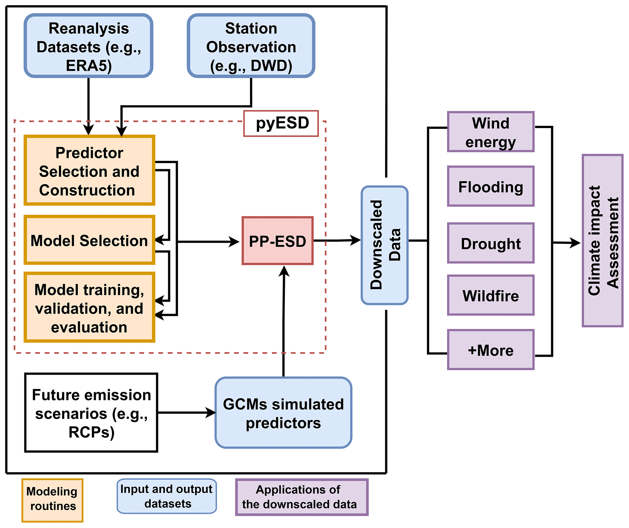
Figure 1The main features and workflow of PP-ESD implemented in the pyESD package (highlighted by the dashed red box). The weather station and reanalysis datasets are used to select the robust predictors for model training and validation. The trained PP-ESD model is then coupled to GCM simulations forced with different scenarios to predict the local-scale future estimates that can be used for climate change impact assessment (not included in the pyESD package).
2.1 Data structure and preprocessing
PP-ESD modeling requires (1) predictand data from weather stations or other observational systems, (2) reanalysis datasets for the construction of predictors, and (3) GCM or RCM output for the construction of simulated predictors if the PP-ESD models are used for downscaling simulated climates. To understand the workflow demonstrated in later sections, the reader needs to be aware of few important package design choices related to data structure and preprocessing.
-
The package adopts the OOP paradigm and treats every predictand data archive (e.g., weather station or glacier) as an object. Since the current version of the package focuses only on station-based downscaling, we will henceforth describe it only as the weather station object. The package accepts the (typical for weather stations) comma-separated value (CSV) file format. These files contain the predictand time series, such as a temperature record, as well as weather station attributes like the weather station's name, ID, and location. The read_station_csv from the pyESD.weatherstation module initiates each weather station as a separate object using the StationOperator that features all the other functionalities. The weather station object is associated with at least one predictand dataset (i.e., the values of at least one climate variable recorded at that particular station). Furthermore, the initialized object includes all attributes and methods required for the complete downscaling cycle. For instance, the package adopts the fit and predict framework of the scikit-learn Python package (Pedregosa et al., 2011) that can be directly applied to the weather station object.
-
The data needed for predictor construction are read from files in the network Common Data Form (netCDF) format with the Xarray toolkit (Hoyer and Hamman, 2017). Due to the size of these datasets and the computations required to construct the predictors, the memory demand can be very high, and repeating this step every time a new model is trained or applied becomes computationally very costly. This problem is circumvented by storing the constructed predictors for each weather station in pickle files. At the next runtime, these can quickly be read (or unpacked) to reduce the computational costs and facilitate faster experimentation with the package.
-
Since reanalysis datasets, climate model output, and weather station data are provided by different data centers and have varied structures and attributes, it is well outside the scope of our project to write and include a unified data processing function for all. Instead, the preprocessing functions of the current version of pyESD are written for state-of-the-art, representative, and publicly available datasets. More specifically, they work with weather station data from the German Weather Service (Deutscher Wetterdienst, DWD) and the ERA5 reanalysis product (Hersbach et al., 2020). These preprocessing functions are provided as part of the package utilities (pyESD.data_preprocess_utils) and can easily be adapted to work for researchers' preferred datasets. The functions will be expanded in the future to allow experimentation with other popular datasets and assess the sensitivity of ESD model performance to the choice of reanalysis datasets (e.g., Brands et al., 2012).
2.2 Predictor selection and construction
The PP-ESD approach is highly sensitive to the choice of predictors and learning models (Maraun et al., 2019a; Gutiérrez et al., 2019). Moreover, since PP-ESD models are empirical in nature, the predictors serve as proxies for all the relevant physical processes and must be informative enough to account for the local predictand variability (Huth, 1999, 2004; Maraun and Widmann, 2018). Therefore, the selection of potential predictors should be informed by our knowledge of the atmospheric dynamics that control the climate variability of the study area. For example, synoptic-scale climate features, such as atmospheric teleconnection patterns, control much of the regional-scale climate variability. It is therefore recommended to consider these as potential predictors. Statistical techniques, such as methods for feature selection or dimension reduction, may then be applied to reduce the list of physically relevant potential predictors to a smaller selection of predictors that have a robust statistical relationship with the predictand. These steps contribute to the performance of the models and also resolve some of the issues related to multicollinearity and overfitting (e.g., Mutz et al., 2016). The pyESD package adopts three different wrapper feature selection techniques that can be explored for different models: (1) recursive feature elimination (Chen and Jeong, 2007), (2) tree-based feature selection (Zhou et al., 2021), and (3) sequential feature selection (Ferri et al., 1994). The methods are included in pyESD.feature_selection as RecursiveFeatureElimination, TreeBasedSelection, and SequetialFeatureSelection, respectively. Furthermore, classical filter feature selection techniques, such as correlation analyses, are also included as a method of the weather station object.
Predictors are typically constructed by (1) computing the regional means of a physically relevant climate variable or (2) constructing index time series for relevant synoptic-scale climate phenomena. The package allows the user to consider a few important aspects for each type of predictor.
-
The area over which the climate variable is averaged can significantly affect model performance. In complex terrain with high-frequency topography, for example, choosing a smaller spatial extent may result in the predictor having a higher explanatory power. Therefore, a radius (with a default value of 200 km) around the weather station may be defined by the user to determine the size of the area used for the computation of the regional means.
-
Empirical orthogonal function (EOF) analysis is a well-established tool for capturing atmospheric teleconnection patterns and reducing high-dimensional climate datasets to index time series that represent the variability of prominent modes of synoptic-scale climate phenomena (Storch and von Zwiers, 2002). The current version of pyESD includes functions for the extraction of EOF-based index time series for dominant extratropical teleconnection patterns in the Northern Hemisphere (pyESD.teleconnections). More specifically, it allows the computation of index values for the North Atlantic Oscillation (NAO) as well as the East Atlantic (EA), Scandinavian (SCAN), and East Atlantic–Western Russian (EAWR) oscillation patterns (e.g., Boateng et al., 2022). It will be expanded to consider Southern Hemisphere patterns in future versions.
After the selection and construction of predictors, their raw values can be transformed before model training. For instance, MonthlyStandardizer implemented in pyESD.standardizer can be used to remove the seasonal trends in each predictor by centering and scaling the data. Such transformation can reduce biases toward high-variance predictors, ensure generalization, and improve the representation of predictors constructed from GCM output (e.g., Bedia et al., 2020; Benestad et al., 2015a). Principal component analysis (PCA) is another transformation tool included in the package (pyESD.standardizer.PCAScaling). It can be applied to (a) reduce the raw predictor values to information that is relevant to the predictand and (b) prevent multicollinearity-related problems during model training (e.g., Mutz et al., 2016).
2.3 Learning models
The empirical relationship between local predictand and large-scale predictors is often complicated due to the complex dynamics in the climate system. However, ML algorithms have been demonstrated to perform well in extracting hidden patterns in climate data that are relevant for building more complex transfer functions (e.g., Raissi and Karniadakis, 2018). Specifically, neural networks have been explored for downscaling climate information due to their ability to establish a complex and nonlinear relationship between predictands and predictors (e.g., Nourani et al., 2019; Gardner and Dorling, 1998; Vu et al., 2016). Moreover, support vector machine (SVM) models have been used to capture the links between predictors and predictands by mapping the low-dimensional data into a high-dimensional feature space with the use of kernel functions (e.g., Anandhi et al., 2008; Tripathi et al., 2006). Previous studies have also applied multi-model ensembles due to their ability to reduce model variance and capture the distribution of the training data (e.g., Xu et al., 2020; Massaoudi et al., 2021; Gu et al., 2022).
Selecting the most appropriate model or algorithm for a specific location or predictand can be challenging because one needs to consider many case-specific factors like data dimensionality, distribution, temporal resolution, and explainability. This problem is exacerbated by the lack of well-established frameworks for climate information downscaling (Gutiérrez et al., 2019). The pyESD package addresses this challenge with the implementation of many ML models that are different with regard to their theoretical paradigms, assumptions, and model structure. The implementation of commonly used models in the same package allows researchers to experiment with different learning models and to replicate and update their research based on emerging recommendations for specific predictands and geographical locations. The implementation of statistical and ML models in pyESD mainly relies on the open-source scientific framework scikit-learn tool (Pedregosa et al., 2011). In the following subsections, we briefly explain the principles behind the ML methods that are included in the pyESD package.
2.3.1 Regularization regressors
Regularization models are penalized regression techniques that shrink the coefficients of uninformative predictors to improve model accuracy and prediction interpretability (Hastie et al., 2001; Tibshirani, 1996; Gareth et al., 2013). The coefficients of non-robust predictors are set to zero by minimizing the absolute values of regression coefficients or minimizing the sum of squares of the coefficients. The former is referred to as L1 regularization and adopted by the least absolute shrinkage and selection operator (LASSO) method. The latter is referred to as L2 regularization and adopted by the ridge regression method. The regularization term (R) and the updated cost function for a linear equation of p independent variables or predictors, Xi, are defined as
for L1 regularization and
for L2 regularization. Therefore, the updated cost function is defined as
where λ is the tuning parameter that controls the severity of the penalty defined in Eqs. (1) and (2), and βi represents the coefficients. The package features implementations of the LASSO and ridge regression using a cross-validation (CV) scheme with random bootstrapping to iteratively optimize λ. These are included as LassoCV and RidgeCV, respectively. The optimization of the cost function in Eq. (3) is usually based on the coordinate descent algorithm to fit the coefficients (Wu and Lange, 2008). The pyESD package also includes an implementation of LassoCV that uses a less greedy version of the optimizer (LassoLarsCV). It is computationally more efficient by using the least angle regression (Efron et al., 2004) for fitting the coefficients.
2.3.2 Bayesian regression
Bayesian regression employs a type of conditional modeling to obtain the posterior probability (p) of the target variable (y), given a combination of predictor variables (X), regression coefficients (w), and random variables (α) estimated from the data (Bishop and Nasrabadi, 2006; Neal, 2012). In its simplest form, the normal linear model, the predictand yi (given the predictors Xj), follows a Gaussian distribution N(μ,σ). Therefore, to estimate the full probabilistic model, yi is assumed to be normally distributed around Xijw:
This approach also permits the use of regularizers in the optimization process. The Bayesian ridge regression procedure (BayesianRidge) estimates the regression coefficients from a spherical Gaussian and L2 regularization (Eq. 2). The regularizer parameters (α,λ) are estimated by maximizing the log marginal likelihood under a Gaussian prior over w with a precision of λ−1 (Tipping, 2001; MacKay, 1992):
This means that the parameters (α, λ, and w in Eqs. 4 and 5) are estimated jointly in the calibration process. Automatic relevance determination regression (ARD) is an alternative model included in the package. It differs from BayesianRidge in estimating sparse regression coefficients and using centered elliptic Gaussian priors over the coefficients w (Wipf and Nagarajan, 2007; Tipping, 2001). Previous studies have used sparse Bayesian learning (relevance vector machine – RVM) for downscaling climate information (e.g., Das et al., 2014; Ghosh and Mujumdar, 2008).
2.3.3 Artificial neural network
The multilayer perceptron (MLP) is a classical example of a feed-forward ANN, meaning that the flow of data through the neural network is unidirectional without recurrent connections between the layers (Gardner and Dorling, 1998; Pal and Mitra, 1992). MLP is a supervised learning algorithm that consists of three layers (i.e., an input, hidden, and output layer) connected by transformation coefficients (weights) using nonlinear activation such as the hyperbolic function. More specifically, the learning algorithm with one hidden layer for the training sets (X1,y1), (X2,y2), …, (Xn,yn), where XiϵRn and yiϵ{0,1}, can be defined as
where θ is the activation function, and b1 and b2 are the model biases added to the hidden and output layer. The weights connecting the layers are optimized with the backpropagation algorithm (Hecht-Nielsen, 1992; Rumelhart et al., 1986) with a mean squared error loss function. Moreover, the L2 regularization (Eq. 2) method is applied to avoid overfitting by shrinking the weights with higher magnitudes. Therefore, the optimized squared error loss function is defined as
where is the L2 penalty that shrinks the model complexity. Often, the derivative of the loss function with respect to the weights is determined until the residual error of the model is satisfactory. The stochastic gradient descent algorithm (Bottou, 1991; Kingma and Ba, 2014) is used as a solver for updating the weights (defined in Eq. 6) in a maximum number of iterations until a satisfactory loss (Eq. 7) is achieved. Moreover, the choice of the parameters, such as the size of hidden layers, activation function, and learning algorithm, is relevant to the performance of the model (Diaz et al., 2017). The exhaustive search algorithm with CV bootstrapping is a simple and efficient method for parameter optimization (Pontes et al., 2016) and therefore included in the pyESD package (GridSearchCV).
2.3.4 Support vector machine
Support vector regression (SVR) uses the principles of SVM as a regression technique. The learning algorithms are based on Vapnik–Chervonenkis (VC) theory and empirical risk minimization that is designed to solve linear and nonlinear problems. This is achieved by applying kernel functions to map low-dimensional data to higher- or even infinite-dimensional feature space (Vapnik, 2000; Cristianini and Shawe-Taylor, 2000). In principle, the model creates a hyperplane in a vector space containing groups of data points. This hyperplane is a linear classifier that maximizes the group margins. Given finite predictor and predictand data points (X1,y1), (X2,y2), …, (Xn,yn), where XiϵRn and yiϵR, the regressor can be defined as
where the support vectors w and model bias b are the optimal parameters that minimize the cost function in Eqs. (9):
subject to
where ξi, , and i=1…n are the slack variables (the upper and lower training errors) subject to the error tolerance of ε that prevents overfitting. C represents a regularization term that determines the balance between minimal loss and maximal margins. The cost function in Eq. (9) is solved using Lagrange's formula (Balasundaram and Tanveer, 2013) to obtain the optimized function:
where αi and are Lagrange multipliers, and ϕ(Xi,Xj) is the kernel function which implicitly maps the training vectors in Eq. (8) into a higher-dimensional space. The SVR method of the pyESD package includes linear, polynomial, sigmoid, and Gaussian radial basis function (RBF) kernels (Hofmann et al., 2008). Moreover, the degree of regularization (C) and the coefficient of the kernels (γ) is given a range of values so that the hyperparameter optimization algorithm can determine the best model. Due to the expensive nature of SVR, the package uses a randomized search algorithm in a CV setting for the hyperparameter optimization (Bergstra and Bengio, 2012). However, hyperparameters optimization algorithms, such as Bayesian and grid search (Snoek et al., 2012; Pontes et al., 2016; Bergstra et al., 2011) methods, are also provided as alternatives. Previous downscaling projects have taken advantage of the SVR method due to its ability to map data into higher-dimensional space and exclude outliers from the training process (Ghosh and Mujumdar, 2008; Chen et al., 2010; Sachindra et al., 2018; Anandhi et al., 2008; Tripathi et al., 2006).
2.3.5 Ensemble machine learning
Each ML technique is associated with challenges that arise from the method's limitations and underlying assumptions. These have to be considered carefully in the evaluation of the resulting downscaling product. Some of these challenges can be overcome by an integration of different ML models for a specific task (Dietterich, 2000; Zhang and Ma, 2012). Integrated ML models have been suggested to outperform single ML models in downscaling climate information (e.g., Liu et al., 2015). Ensemble models typically use different ML algorithms (base learners) to extract information from the training data, then use a second set of ML algorithms (meta-learners) that learn from the first and combine the individual predictions into an ensemble. Ensemble models can be categorized by (a) the selection of base learners and (b) the method of combining the individual predictions from the base learners. Here, we summarize the more prominent ensemble models that are included in the pyESD package.
Bagging
Bagging ensemble models consist of ML algorithms that generate several instances of base learners using random subsets of the training data and then aggregate the information for the final estimates (Breiman, 1996a; Quinlan, 1996). Such algorithms integrate randomization into the learning process and thereby often ensure the reduction of the variance of the individual base learners (e.g., decision trees). Moreover, bagging techniques constitute a simple way to improve model performance without the need to adapt the underlying base algorithm. Since bagging works well with complex algorithms like decision trees, we also consider tree-based ensembles for the pyESD package. More specifically, we include implementations of the random forest (RandomForest) and extremely randomized tree (ExtraTree) methods in addition to classical bagging.
The RandomForest algorithm builds multiple independent tree-based learners. The trees can be constructed with the full set of predictors or a random subset. Each tree is constructed from a random sample of the training data in a bootstrapping process (Breiman, 2001). The algorithm uses the remaining training data (i.e., out-of-bag data) to estimate the error rate and evaluate the model's robustness. In contrast, the ExtraTree algorithm considers the discriminative thresholds from each predictor rather than the subset of predictors (Geurts et al., 2006). This usually adds more weight to the variance reduction and slightly improves the model bias. Tree-based ensembles are particularly suitable for establishing a nonlinear relationship between predictors and predictands (e.g., Pang et al., 2017; He et al., 2016).
Boosting
In recent years, boosting models have also been applied for the downscaling of climate information (e.g., Fan et al., 2021; Zhang et al., 2021). Boosting models are meta-estimators that are built sequentially from multiple base learners with the primary objective of reducing the model bias and variance. In principle, the method “boosts” weaker base learners (i.e., estimators that perform only slightly better than random guessing) by converting them into strong ones in an iterative process. The technique assumes that the base learning model is distribution-free (Schapire, 1999) and iteratively improves the weaker base learners by applying weights to the training data through the adjustment of the input points with prediction errors from the previous prediction (Schapire, 2003; Schapire and Freund, 2013). There are many boosting algorithms due to the many possible methods of weighting the training data and tuning the weaker base learners. In the pyESD package, we include (1) adaptive boosting (Adaboost), (2) gradient tree boosting (GradientBoost) with a gradient boosting algorithm by Friedman (2001), and (3) extreme gradient boosting (XGBoost). A brief summary of each is provided below.
-
The Adaboost algorithm is a well-established model for improving the accuracy of weak base learners (Freund and Schapire, 1997). The model is adaptive in the sense that the training data are sequentially adjusted based on the previous performance of the weaker model. The model uses a weighted majority vote (or sum) to combine the individual prediction from the weaker learners and produce a robust final prediction. The implemented version uses a decision tree algorithm as the base estimator to develop the boosted ensemble predictions.
-
The GradientBoost algorithm considers the boosting process to be a numerical optimization problem that minimizes a loss function in a stage-wise additive model by adding weaker learners using a gradient descent procedure. This generalization allows the tuning of an arbitrary differentiable loss function which can be selected based on a specific problem. Specifically, in pyESD, squared errors are used in the minimization of the loss function.
-
XGBoost, a recent extension of the GradientBoost algorithm, is designed to reduce computational time and improve model performance (Chen and Guestrin, 2016). The model uses regularization terms to penalize the final weights and prevent overfitting. The algorithm also uses shrinkage and column subsampling techniques to avoid overfitting. Moreover, the model can handle sparse data by using a sparsity-aware split function.
Stacked generalization
The stacked generalization method (or “stacking”) has previously been used for the downscaling climate information and has shown improved prediction robustness over singular models (e.g., Massaoudi et al., 2021; Gu et al., 2022). It is designed to enhance prediction accuracy and generality by taking advantage of the mutual complementarity of the base-model predictions. The approach was introduced by Wolpert (1992) and demonstrated for regression tasks and unsupervised learning by Breiman (1996b) and Leblanc and Tibshirani (1996), respectively. In principle, the following process is implemented: in the first step, the training data and base models, referred to as level-0 data and level-0 models by Wolpert (1992), are used to generate the first set of predictions. Then a meta-learning model (level-1 generalizer) is used to optimally combine the previous predictions (level-1 data) into final estimates. Lastly, the method applies a cross-validation technique and generates new “stacked” datasets for a final learning step. Generally, the performance of stacked generalization is constrained by the attributes used to generate the level-1 data and the type of algorithm used for higher-level learning (Ting and Witten, 1999). We consider these limitations by providing a wide range of models that can be used as the level-0 models and the level-l generalizer. The base learners can be selected from the different ML models presented in the previous sections. The reader is advised that previous studies (e.g., Reid and Grudic, 2009) suggest the use of a more restrictive model like LassoCV and ExtraTree as the meta-learner to prevent overfitting.
2.4 Model training
The process of training and testing the PP-ESD models is the most critical stage in the downscaling procedure, since it determines much of the robustness of the final models, as well as the accuracy of the predictions they generate. The process typically involves the following steps: (1) the observational records are separated into training and testing datasets. (2) The training datasets are used to establish the transfer functions that make up the PP-ESD models. (3) The trained models are then evaluated on the independent testing datasets (Sect. 2.5). In the model training process, hyperparameter optimization techniques (e.g., GridSearchCV) are used to fine-tune the transfer function parameters, such as regression coefficients, to optimize model performance. Cross-validation (CV) techniques are applied to split the whole training dataset into smaller training and validation data sections and allow the assessment and iterative improvement of the model parameters during training while also preventing overfitting (Moore, 2001; Santos et al., 2018). In this category of techniques, the k-fold framework is the most used for climate information downscaling models. It partitions the training data into k equally sized and mutually exclusive subsamples, which are also referred to as folds (Stone, 1976; Markatou et al., 2005). More specifically, for each iteration step, one fold is used for model validation, and the remaining k−1 folds are used for model training. The leave-one-out CV technique (Lachenbruch and Mickey, 1968) is an alternative and has been used for the development of ESD models (e.g., Gutiérrez et al., 2013). Cross-validation techniques rely on the fundamental assumption of independent and identically distributed (i.i.d) data. They, therefore, treat the data as a result of a generative process that has no memory of previously generated samples (Arlot and Celisse, 2010). The assumption of i.i.d might not be valid for time series data (e.g., Bergmeir and Benítez, 2012) due to seasonal effects, for example. To circumvent this problem, monthly bootstrapped resampling and time series splitters are included in the pyESD package. The pyESD.splitter module contains all CV frameworks available for model training, including the k-fold, leave-one-out, and other CV schemes. The validation metrics used for optimizing the model parameters include the coefficient of determination (R2) (Eq. 11), root mean squared error (RMSE) (Eq. 13), mean absolute error (MAE) (Eq. 14), and others that are summarized in Sect. 2.5. The final values for the validation metrics, which reflect the model performance during training, are arithmetic means of the individual values for each iteration. In this paper, we refer to them as CV performance metrics (i.e., CV R2, CV RMSE, and CV MAE).
2.5 Model evaluation
In the process of downscaling climate information, best practice involves the use of stringent model evaluation schemes with independent data outside the training data range (Wilby et al., 2004). Retaining a section of the data as a testing dataset (Sect. 2.4) is recommended if longer records (e.g., ≥30 years) are available. It allows (a) a completely independent evaluation of the trained model's performance and (b) an assessment of the sensitivity of the model to the chosen training dataset. In the case of time series, the latter can provide insights into the model's sensitivity to the calibration period and the temporal stationarity of the model's transfer functions. If the records are short (e.g., <30 years), the CV metrics (Sect. 2.4) can be used, albeit with caveats, as nonideal estimates for the model's performance (e.g., Mutz et al., 2021). For the remainder of this section, however, we will assume that longer records and completely independent testing datasets are available.
The PP-ESD model is evaluated on the basis of the model's predictions and the observed values y. In pyESD, the following performance metrics are implemented.
-
The coefficient of determination (R2) represents the fraction of the predictand's observed variance that can be explained by the predictors. It can be seen as a measure of how well the model predicts the unseen data (Wilks, 2011). The R2 for the predicted values in relation to the observed data yi for i=1, …, n samples is defined as
where is the mean of the observed data, is the sum of squared residuals (SSR), and is the total sum of squares (SST). R2 can range from −∞ to 1, where 1 is the best possible score and negative values are indicative of an arbitrary, worse model. An R2 value of 0 is indicative of a model that would always predict the . In this case, the model represents no improvement over simply using the mean as a model.
Pearson's correlation coefficient (PCC) evaluates the linear correlation between the model predictions yi and observed data xi. The PCC of 1 indicates a perfect positive correlation, −1 indicates a perfect anticorrelation, and 0 indicates no correlation between the predicted and observed values. The PCC for n samples is defined as
where the and are the means of the xi and xi values, respectively.
The root mean squared error (RMSE) estimates the mean magnitude of error between the predictions and observations. The RMSE is given in the physical units of the observed data and not standardized. Smaller values indicate better model performance. The RMSE for predictions and observations yi of n samples is calculated as
The mean absolute error (MAE) is a scale-dependent accuracy measure that also provides information on the errors between the predictions and observations. The MAE is estimated as the sum of absolute errors normalized by the sample size (n). The MAE is calculated as
Additional metrics such as the mean squared error (MSE), mean absolute percentage error (MAPE), maximum error, adjusted R2 (Miles, 2014), and Nash–Sutcliffe efficiency (NSE) (Nash and Sutcliffe, 1970) are included in pyESD. However, the predicted values from the trained model and their corresponding observed values can be evaluated using other metrics not included in pyESD. For example, additional metrics like the model skill score E and the revised R2 (RRS), which combines correlation, bias measure, and the capacity to capture variability, can be used (Onyutha, 2021). We highlight that the limitations and assumptions underpinning these metrics should be considered when interpreting performance metrics. For example, the RMSE is sensitive to outliers because the squaring of errors assigns more weight to large errors. This implies that a single outlier can bias its estimate and lead to a misinterpretation of extreme data points in the predictand. Although MAE is less sensitive to outliers compared to RMSE, its treatment of all errors with equal weight may not adequately account for the impact of extreme errors on model performance. Consequently, both metrics should be interpreted with respect to the mean of the observed values. On the other hand, the Pearson correlation coefficient (PCC) assumes a linear relationship between the predicted and observed values and a bivariate normal distribution. However, distance correlation (Székely et al., 2007), which is more computationally demanding and makes no assumptions about the relationship or distribution, can be considered. Chaudhuri and Hu (2019) demonstrated a fast algorithm that can be used to compute the distance correlation.
2.6 GCM–ESD coupling and local-scale predictions
The developed and tested PP-ESD model can finally be coupled to coarse-scale climate information. If the PP-ESD model was developed with the intention to downscale predictions of future climate change, the next logical step is to couple it to GCM simulations forced with different greenhouse gas concentration scenarios. Since PP-ESD is the bias-free downscaling alternative to MOS-ESD, PP-ESD models may be coupled to all GCMs, provided that the predictors are adequately represented by the GCMs. This condition may be alleviated to an extent by standardizing the simulated predictor (Bedia et al., 2020). An analysis of the distribution similarity between the observed and simulated predictors can be conducted to test the assumption of representation. For example, the Kolmogorov–Smirnov (KS) test, which is implemented as part of the pyESD package utilities, is a nonparametric statistical hypothesis test that can be used to evaluate the null hypothesis (H0) that the observation-based predictors and simulated predictors are of the same theoretical distribution.
The first step in ESD–GCM coupling is to utilize the GCM output to recreate the predictors used in the training of the ESD model. This may involve anything from constructing simple temperature regional means to reconstructing multivariate indices for more complex climate phenomena. In the case of index-based predictors such as NAO, EA, SCAN, and others, the simulated indices are reconstructed by projecting the pressure anomalies of the GCM onto the EOF loading patterns of the predictors (e.g., Mutz et al., 2016). This ensures that the physical meaning of the index values is maintained. The ESD model then takes these simulated predictors as input and generates local-scale predictions according to the model's transfer functions. The added value of the resulting downscaling product can be evaluated by comparing the downscaled values to the raw outputs of different GCMs and RCMs. Finally, the high-resolution local-scale predictions can be used to drive climate change impact assessment models to predict flood frequency (e.g., Padulano et al., 2021; Hodgkins et al., 2017), agricultural changes (e.g., Mearns et al., 1996), changes in water resources (e.g., Dau et al., 2021), and more.
We demonstrate the complete downscaling workflow and highlight most of the functionalities of the pyESD package in an illustrative case study. The study uses the PP-ESD approach and is set in the Neckar catchment, a hydrological catchment in southwestern Germany that consists of complex mountainous terrain with topographic elevations between 200 and 1000 m above sea level (Fig. 2). The region is climatically complex, since local climates are influenced by atmospheric teleconnection patterns (e.g., NAO, EA, and SCAND), orographic effects (e.g., Kunstmann et al., 2004), and the Mediterranean climate (Bárdossy, 2010; Ludwig et al., 2003). The catchment experiences maximum precipitation (80–120 mm per month) and temperature (15–18 ∘C) in the summer months (Fig. 3). The catchment serves as a water supply for drinking and agricultural activities (Selle et al., 2013). We use this catchment for our case study because (a) it is a suitable region to test the strengths and limitations of the pyESD downscaling package, and (b) generating 21st century climate change estimates can contribute to regional climate impact assessments and adaptation.
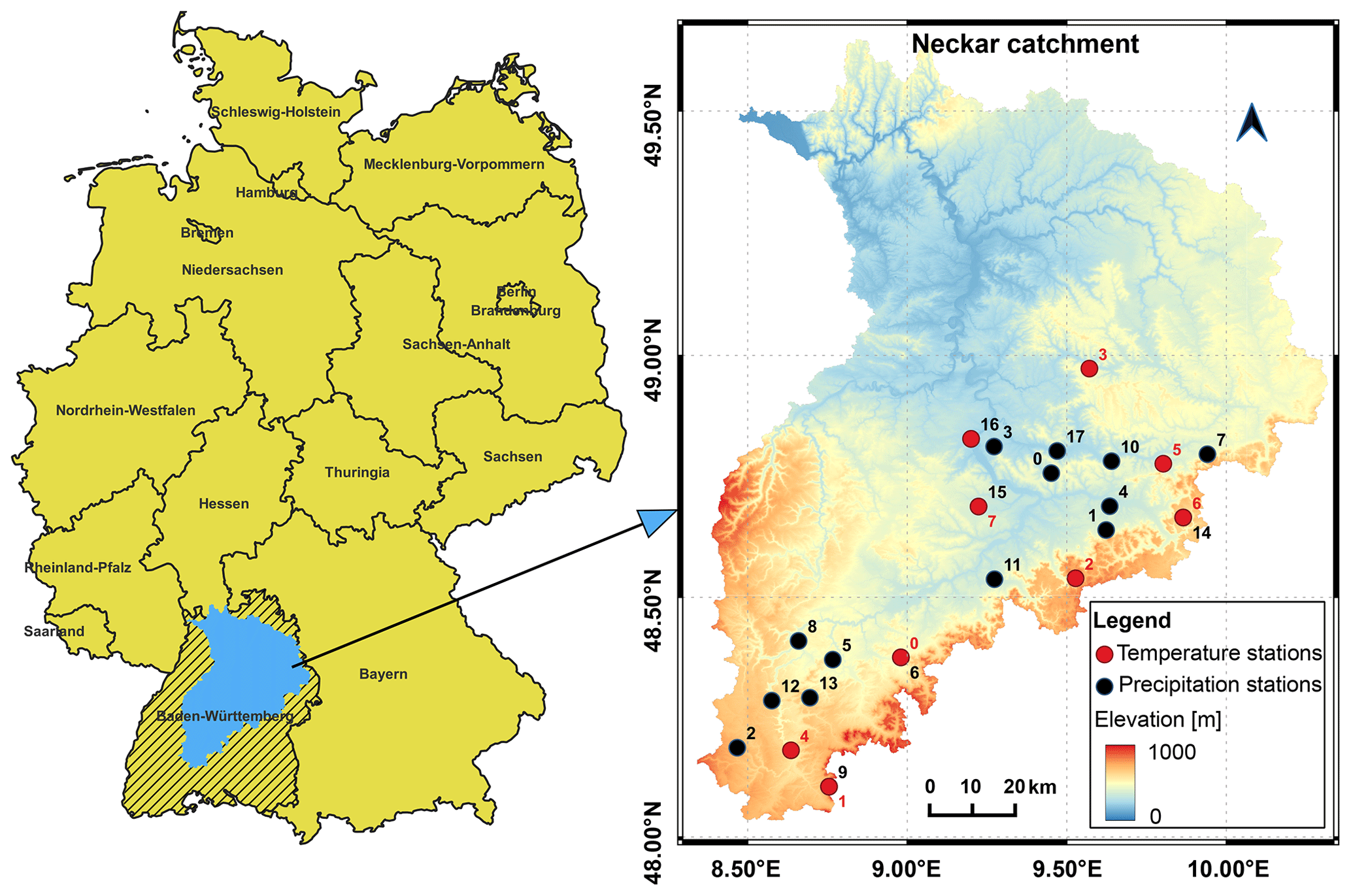
Figure 2Weather station locations and elevations in the Neckar catchment. The red circles represent temperature stations (ID corresponds to Table 1b), and the black circles represent precipitation stations (ID corresponds to Table 1a). The color map shows the elevation and delineates the extent of the catchment.
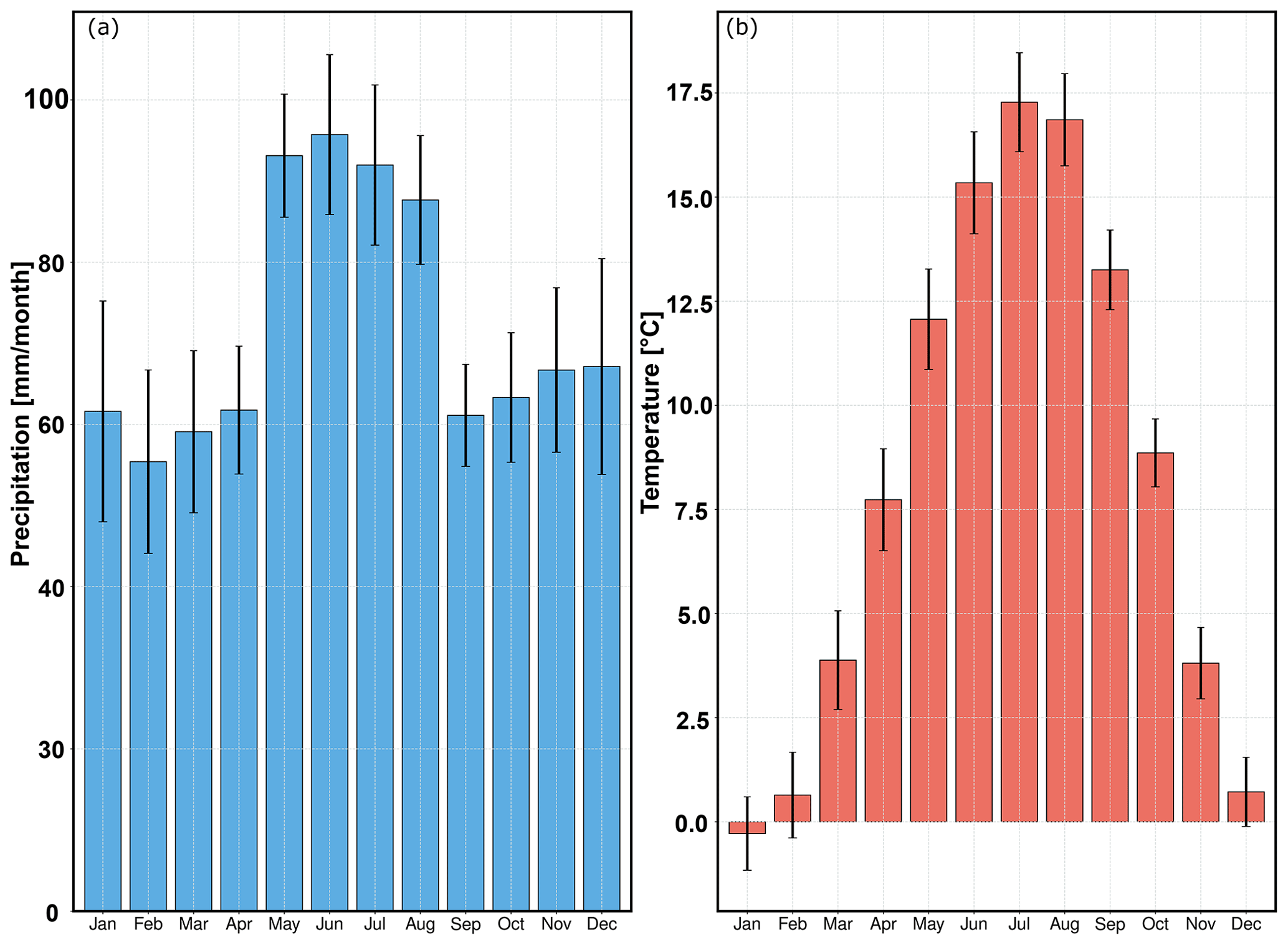
Figure 3Long-term (1958–2020) monthly means of (a) precipitation and (b) temperature, averaged over all stations in the catchment. The error bars are the standard deviations that represent inter-station variability. The maximum precipitation and temperature in the catchment are recorded in the summer season (JJA).
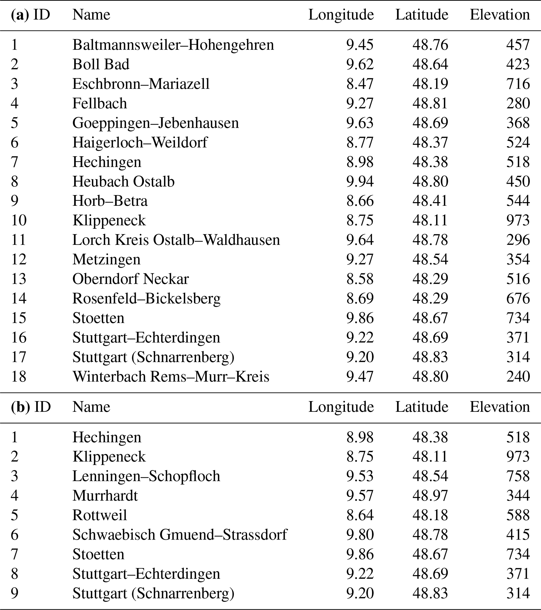
In this case study, we apply pyESD to predict local temperature and precipitation changes for 22 weather stations located in the catchment (Table 1) and demonstrate the package's flexibility by performing experiments with the different modeling alternatives. We show most of the PP-ESD steps required for generating robust downscaling products. These steps include (1) predictor selection and construction; (2) model selection, training, and cross-validation; (3) model evaluation; and (4) generating future predictions through ESD–GCM coupling (see Sect. 3.2 for details). We note that the focus of the case study is more on demonstrating the pyESD workflow and functionality and less on detailed discussions of the downscaled results and their implications. In order to allow readers to reproduce and learn from this application example, we only use public and freely available datasets (see Sect. 3.1 for more details about the data). Moreover, all scripts used in this study (i.e., data preprocessing, modeling, and visualization scripts) are provided in the code and data availability section.
Table 1IDs (specific to this study), names, coordinates, and elevation (m) for weather stations recording (a) precipitation and (b) temperature.
3.1 Datasets
3.1.1 Weather station data
Monthly precipitation and temperature station data from the German Weather Service (Deutscher Wetterdienst, DWD accessible from https://cdc.dwd.de/portal/, last access: 30 October 2023) served as the predictand time series in this study. We considered all weather station records that (a) originated from measurements in the Quelle–Enz subcatchment, (b) covered the time period of 1958 to 2020, and (c) were at least 30 years in length. Even though there is no well-established and universally valid recommendation for the minimum record length in a PP-ESD approach (e.g., Hewitson et al., 2014), we chose a conservative 30-year threshold to ensure the models can be evaluated with truly independent, retained data (see Sect. 2.5). The remaining weather stations are summarized in Table 1. These were loaded into predictand station objects (SOs) as follows.
1 from pyESD.Weatherstation import read_station_csv
2 variable = "Temperature" #or 'Precipitation'
3 SO = read_station_csv(filename, variable)
3.1.2 Reanalysis datasets
The ERA5 reanalysis products, produced and managed by the European Centre for Medium-Range Weather Forecasting (ECMWF), were used to construct the predictors in this study. ERA5 is based on historical records from various observational systems (e.g., oceans buoys, aircraft, weather stations) that are dynamically interpolated with numerical forecasting models in a four-dimensional variational (4D-Var) data assimilation scheme to generate global, homogeneous, spatially gridded datasets (Bell et al., 2021). It has a spatial resolution of approximately 31 km (or TL639) and is available as hourly data, covering 1950 to the present day with a 5 d lag of data availability (Hersbach et al., 2020). For this study, however, mean monthly values were used in the construction of potential predictors (Table 2). These are publicly available from the Copernicus Climate Data Store (CDS) (accessible at https://cds.climate.copernicus.eu, last access: 30 October 2023).
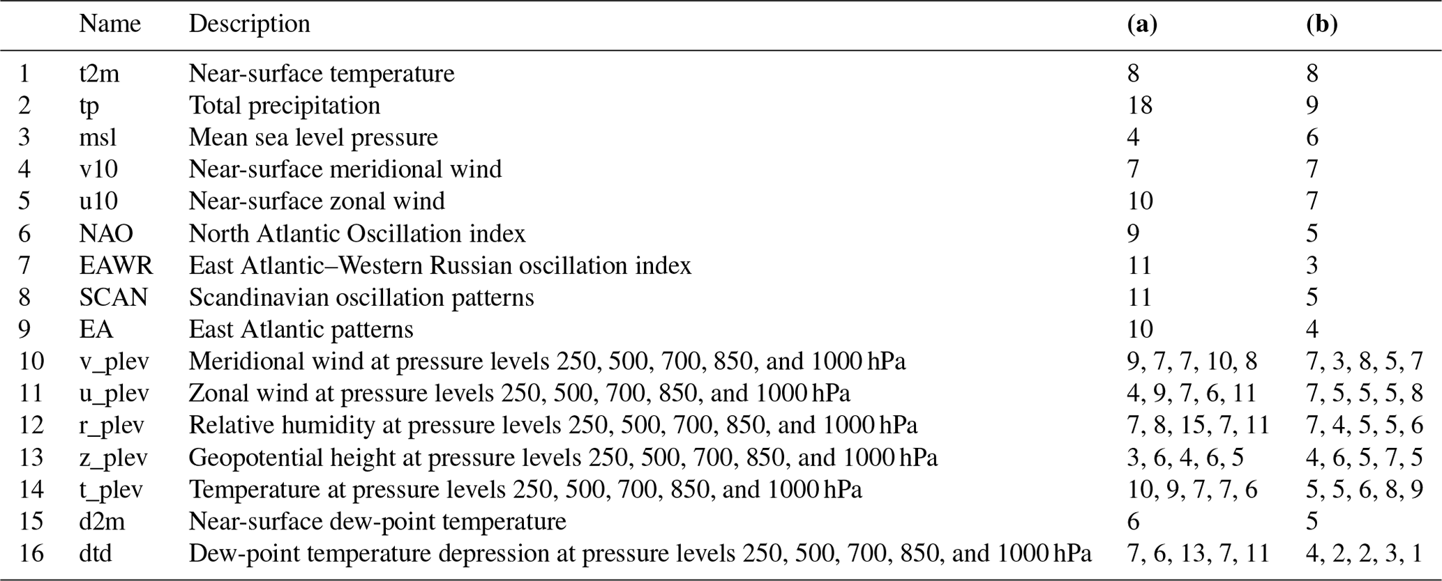
Table 2Potential predictors considered for PP-ESD models and the frequency of their selection for (a) precipitation and (b) temperature stations (based on the final predictor selection method).
3.1.3 GCM simulation datasets
For the ESD–GCM coupling, the predictors were reconstructed from an MPI-ESM (Max Planck Institute Earth System Model) GCM simulation that follows the protocols of the World Climate Research Programme's (WCRP) Coupled Model Intercomparison Project phase 5 (CMIP5) (Taylor et al., 2012). We highlight that CMIP5 model output was chosen in this illustrative study to enable consistent comparison with previous regional climate models over the region and any GCM outputs (e.g., CMIP6) can be combined with pyESD. For the case study, we consider several simulations (accessible at https://cds.climate.copernicus.eu, last access: 30 October 2023) forced with different RCP scenarios (Moss et al., 2010) to predict the local-scale response to the plausible range of forcings. In order to highlight the added value of the downscaled product, the local-scale future estimates are compared to the coarser predictions of several GCMs (i.e., MPI-ESM, CESM1-CAM5 of the National Center for Atmospheric Research – NCAR, Kay et al., 2015, and HadGE2-ES of the Hadley Centre of the UK Met Office, Collins et al., 2008) and RCMs (CORDEX-Europe simulation with MPI-CSC-REMO2009 driven with boundary conditions from MPI-ESM).
3.2 Methods
3.2.1 Predictor selection and construction
The considered predictors must be large-scale climate elements that are both physically and empirically relevant to predicting the local-scale climate variability in the vicinity of the weather station. The physical relevance of considered predictors (Table 2) is established through previous studies and general climatological merit. We then apply a monthly standardizer transformer to remove the seasonality trends and scale the individual predictors. The empirical relationship with the predictand is then evaluated with PCCs defined in Eq. (12). Finally, first estimates of their predictive skills are obtained through the application of the package's recursive, sequential, and tree-based algorithms in a CV setting. These preliminary experiments are conducted to refine the selection of predictors further. After the predictor selection process, each weather station and predictand is associated with a particular subset of predictors (Table 2) that are later used to train the final ESD model for the station (Sect. 3.2.2).
The steps above are implemented with pyESD as follows.
-
We create a list (predictors) of all considered predictors with physical relevance to the predictand. We then use the set_predictors method of the station object (SO) to read the data in the local directory (predictordir) and construct regional means with a defined radius of 200 km around the station location. These are regional means of relevant climate variables and serve as the simplest type of predictor. For the construction of indices for atmospheric teleconnection patterns (i.e., NAO, EA, SCAN, and EAWR), which serve as further predictors, the package automatically calls the pyESD.teleconnections module if the pattern's acronym is included in the list of predictors.
1 predictors = ["t2m", "tp", "NAO"
,..., "nth predictor"]
2 SO.set_predictors(variable,
predictors, predictordir,
radius=200) # radius in km -
We apply the monthly standardizer and then use the predictor_correlation method to estimate the PCC between the predictand and predictors.
1 SO.set_standardizer(variable,
standardizer = MonthlyStandardizer
(detrending=True, scaling=True))
2 df_corr = SO.predictor_correlation
(variable, predictor_range,
ERA5Data, fit_predictors=True,
fit_predictand=True,
method="pearson") -
The final refinement of the predictor list is implemented as part of the fit method. We use the set_model method to define the ARD regressor, TimeSeriesSplitter CV setting, and call the fit method in a loop through the three types of selector methods.
1 SO.set_model(variable, method="ARD",
cv=TimeSeriesSplit(n_splits=10))
2 selector_methods = ["Recursive",
"TreeBased", "Sequential"]
3 for selector_method in
selector_methods:
4 SO.fit(variable, predictor_range,
ERA5Data, fit_predictors=True,
predictor_selector=True,
selector_method =
selector_method, select_regressor)
3.2.2 Model training and validation
Model training and validation are performed separately for each predictand and weather station. The models are trained in a CV setting for the period 1958–2010 and then assessed on independent retained data for the period 2011–2020. In the training process, we use seven different methods before deciding on an estimator for the final model. These methods include at least one representative for each of the families of ML algorithms (see Sect. 2.3) except SVR. We exclude SVR due to its high computational demands for optimization and to ensure the easy reproducibility of the illustrative example on less powerful computers. We perform the initial model training and validation with the LassoLarsCV, ARD, MLP, RandomForest, XGBoost, bagging, and stacking regressors using a KFold(n_splits=10) validation scheme for hyperparameter optimization. For the stacking regressor, we use all the other regressors as base estimators (i.e., level-0 learners) and ExtraTree as the meta-learner. The final ESD model is then selected based on the CV metrics (i.e., CV R2 and CV RMSE) of the individual models.
The steps above are implemented with pyESD as follows: the models are trained with the fit method as described within Sect. 3.2.2. The cross_validate_and_predict method is applied to calculate the CV metrics and generate the predictions for the training period 1958–2010. The predict method is then used to generate predictions for the 2011–2020 period from the models trained in the 1958–2010 period. Finally, the evaluate method is used to obtain the model performance metrics based on the 2011–2020 predictions and retained data. The R2, RMSE, and MAE (see Sect. 2.5) are used as both CV and evaluation metrics in this study. The ERA5 reanalysis product is specified as the predictor dataset for all these methods.
1 cv_score_1958to2010, predict_1958to2010 = SO.cross_validate_and_predict(variable, from1958to2010, ERA5Data)
2 predict_2011to2020 = SO.predict(variable, from2011to2020, ERA5Data)
3 scores_2011to2020 = SO.evaluate(variable, from2011to2020, ERA5Data)
3.2.3 Future prediction
Future predictions are generated by coupling the final ESD models to GCM simulations for the 21st century. In the illustrative example, we use MPI-ESM simulations that were forced with greenhouse gas concentration scenarios RCP2.6, RCP4.5, and RCP8.5. This coupling is achieved as follows: the predictors selected during model training are reconstructed from the GCM output. These simulated predictors are standardized with the MonthlyStandardizer parameters obtained from the reanalysis predictors to ensure data homogenization. Prediction anomalies are calculated using the training period 1958–2010 as a reference. The resulting RCP-specific 21st century prediction anomaly time series are then used to calculate the annual means (2020–2100), as well as the seasonal (DJF, MAM, JJA, SON) and annual 30-year climatologies for the mid-century (2040–2070) and the end of the century (2070–2100). The predicted anomalies are then back-transformed to their respective absolute values for all stations and compared to the raw outputs of GCMs (i.e., CESM1-CAM5, HadGE2-ES, EURO-CORDEX, and MPI-ESM; see Sect. 3.1.3) using the nearest grid point. In pyESD, a future prediction can be generated by using the predict method (Sect. 3.2.2) and specifying the GCM output as the predictor data source.
The PP-ESD approach relies on the assumption that the predictors are well-represented by the GCM. We therefore perform KS tests to evaluate the distribution similarity between GCM and ERA5 predictors for the datasets' temporal overlap. The KS statistic lies within the 0–1 range, with lower values indicating greater distribution similarity. For our two-sided tests, we reject the null hypothesis (H0 means the datasets have identical underlying distributions) in the case of p values being smaller than 0.05. We perform the test on the raw monthly time series, monthly anomalies, and standardized anomalies in order to isolate the distributional differences of the first and second moments error propagation (Bedia et al., 2020). The KS_stat function implemented in the pyESD.utils module is used to test several of the informative predictors (such as tp, t2m, r850, u850, and v850).
In this section, we present and discuss the results of the illustrative case study. The discussion places more emphasis on the functionalities of the package than the climatological implications. Specifically, we discuss the results of the predictor selection step (Sect. 4.1), the training and validation of the model (Sect. 4.2), the final model performance (Sect. 4.3), and the future predictions generated through the ESD–GCM coupling (Sect. 4.4).
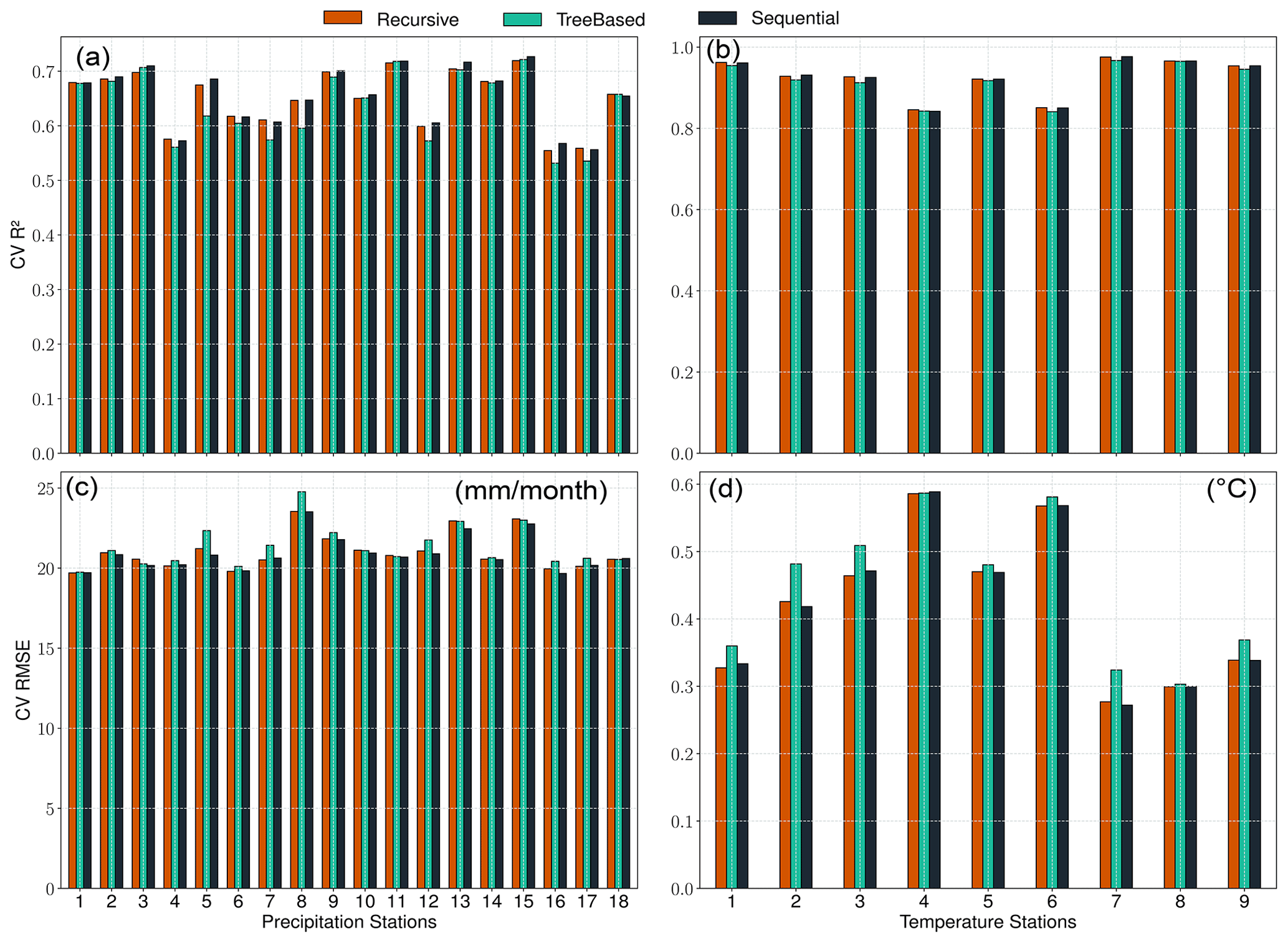
Figure 4Cross-validation R2 and RMSE for the predictor selection methods (recursive in red, tree-based in green, and sequential in black) for precipitation (a, c) and temperature (b, d) station records. The individual methods performed similarly well, suggesting that each of the implemented methods may be used to refine the list of potential predictors.
4.1 Predictor selection
All implemented predictor selection methods demonstrated merit, and the correlation analyses revealed strong linear dependencies between the predictand variables and potential predictors (Figs. A1 and A2). For example, precipitation records are highly correlated (PCC ≥0.5) with large-scale total precipitation (tp), atmospheric relative humidity (r), and zonal wind velocity (u) up to the mid-tropospheric level (i.e., 500–1000 hPa) (Fig. A1). The temperature records are highly correlated (PPC ≥0.7) with near-surface temperature (t2m), atmospheric temperature (t on all levels), and dew-point temperature depression (dtd) up to the mid-troposphere (Fig. A2). Both predictands also show a good correlation (PCC ≥0.25) with the indices of the atmospheric teleconnection patterns (i.e., NAO, EA, EAWR, and SCAN). The predictor selection methods (i.e., recursive, tree-based, and sequential) perform similarly for all the precipitation and temperature stations (Fig. 4). More specifically, the three methods yield CV R2 values of 0.5 to 0.75 (Fig. 4a), CV RMSE values of ≤25 mm per month (Fig. 4c) for precipitation, CV R2 values of ≥0.95 (Fig. 4b), and CV RMSE values of 0.3 to 0.6 ∘C (Fig. 4d) for temperature stations. Since the methods did not show a significant difference in performance, the recursive method was applied for the refinement of the set of predictors, since it allows more flexibility and a stepwise iteration of several combinations of potential predictors (e.g., Mutz et al., 2021; Hammami et al., 2012; Li et al., 2020). The frequencies with which specific predictors were selected using the recursive method are listed in Table 2.
The predictors tp and t2m were included for most of the precipitation and temperature station records, respectively. This indicates that variations in the larger-scale precipitation and temperature fields already explain much of the local-scale predictand variability in the vicinity of the weather stations. Many of the refined predictor sets also included indices of the NAO (9 of 18 precipitation stations, 5 of 9 temperature stations), SCAN (11 of 18 precipitation stations, 5 of 9 temperature stations), EA (10 of 18 precipitation stations, 4 of 9 temperature stations), and EAWR (11 of 18 precipitation stations, 3 of 9 temperature stations). This confirms the strong manifestation of Northern Hemisphere atmospheric teleconnection patterns in the local-scale precipitation and temperature in the catchment (e.g., Bárdossy, 2010; Ludwig et al., 2003). Their exclusion from the other stations is likely due to the fact that their variability might already be captured by zonal and meridional wind speeds and synoptic pressure variables like geopotential height (z) and mean sea level pressure (slp) (Hurrell and Van Loon, 1997; Hurrell, 1995; Barnston and Livezey, 1987; Maraun and Widmann, 2018). Relative humidity was selected as a predictor for most of the precipitation stations. This is consistent with the results of many other studies (e.g., Gutiérrez et al., 2019; Hammami et al., 2012) and our physical understanding of it as a measure of humidity that takes saturation vapor pressure into consideration.
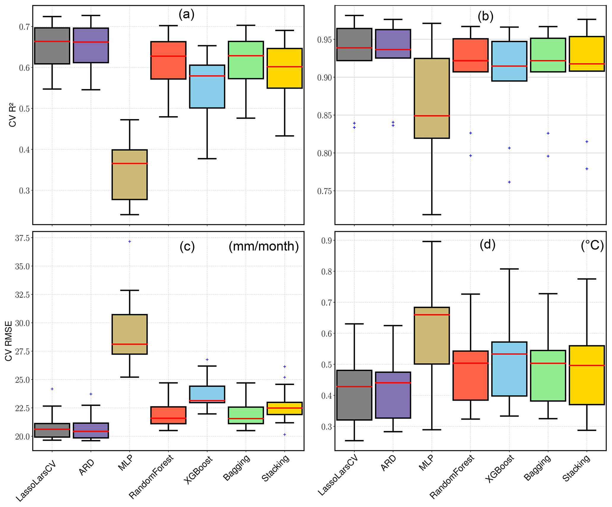
Figure 5Cross-validation R2 and RMSE box plots comparing the experimental regressors' performance for all the precipitation (a, c) and temperature (b, d) stations. The red lines inside the box represent the median, the lower and upper box boundaries indicate the 25th and 75th percentiles, and the lower and upper error lines show the 10th and 90th percentiles, respectively. The black plus marks show the outliers outside the range of the 10th and 90th percentile.
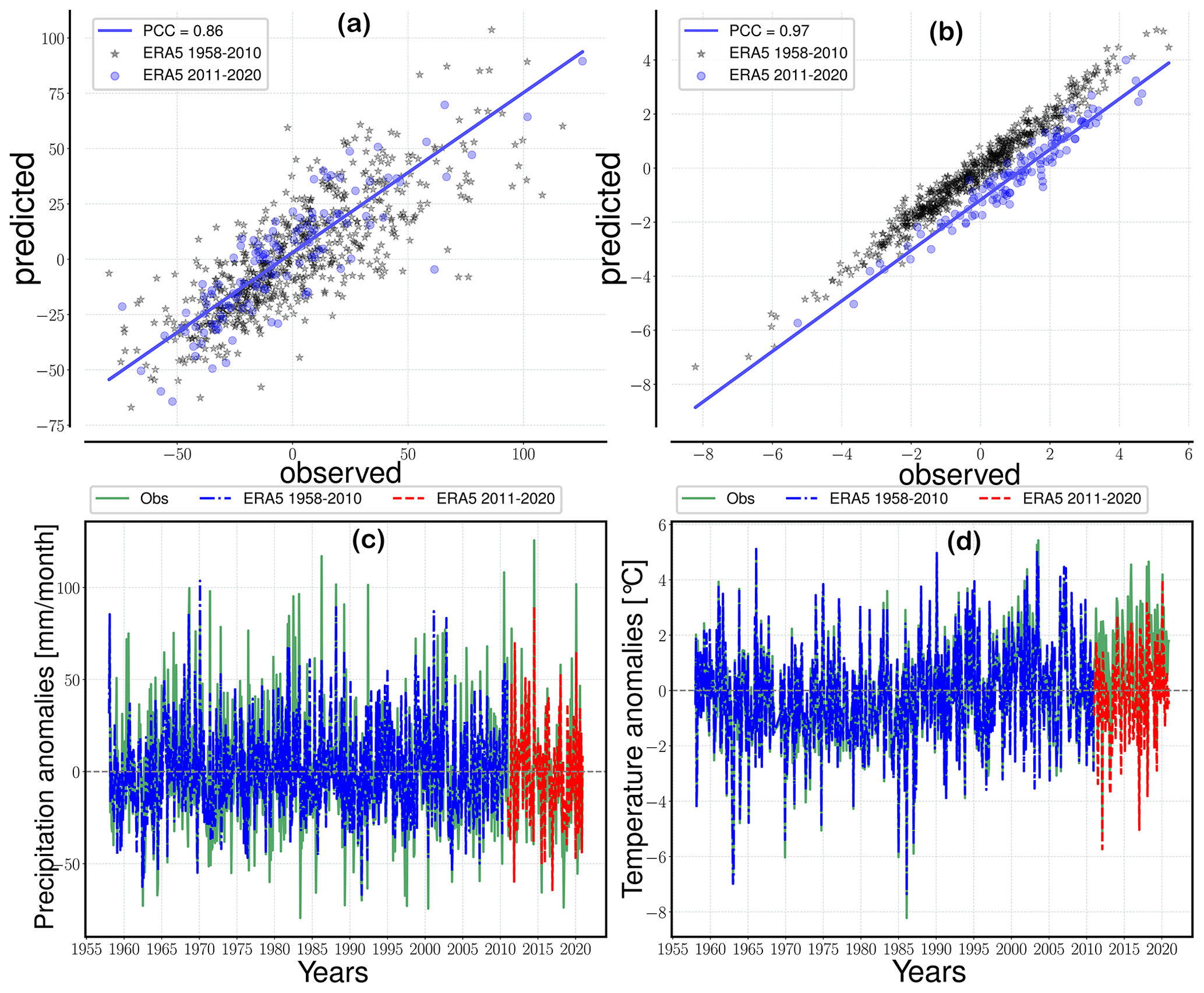
Figure 6Prediction example for the Hechingen station using the final regressor for precipitation (a, c) and temperature (b, d). The top panels (a, b) show the linear relationship between the predictions and observed values, as well as the PCC (R value) for the testing data (blue-colored circles). The bottom panels (c, d) show the 1-year moving average of the observed (green, solid) and ERA5-driven predictions for the training period (blue, dash-dotted) and the testing period (red, dashed).
4.2 Performance of individual estimators
We experimented with seven different regressors before deciding on the regressor that would be used to establish the final ESD models (see Sect.3.2.2). A total of 126 precipitation and 63 temperature experimental models were generated with the seven regressors. Overall, most of the experimental models performed reasonably well with a mean CV R2 of ≥0.5 for precipitation and ≥0.9 for temperature stations (Fig. 5). The MLP models, on the other hand, performed relatively poorly with CV R2 values of ≤0.4 for precipitation and ≤0.9 for temperature. This is due to the fact that MLP model calibration requires longer records and a more complex architecture to capture most of the informative patterns in the training data. This study, however, uses a simplified architecture to make the results reproducible without higher computational requirements. The result can likely be improved with more data (e.g., by using daily values) and an increase in hidden layers (Sect. 2.2.3). The overall performance of the experimental models underlines the methods' suitability for downscaling.
Among the better-performing precipitation models, the LassoLarsCV and ARD methods yielded the best results (CV R2=0.55–0.75, CV RSME = 20–23 mm per month), followed by the RandomForest and bagging ensembles (CV R2=0.48–0.70, CV RSME = 21 to 25 mm per month), as well as the XGBoost ensemble regressor (CV R2=0.39–0.65, CV RMSE = 22–27 mm per month). Stacking all experimental models into a meta-regressor also yields good results (CV R2=0.45–0.7, CV RMSE = 20–26 mm per month) despite the poor performance of the MLP regressors. Based on these results, the LassoLarsCV, ARD, RandomForest, and bagging regressors were selected as the final base learner for the stacking model. ExtaTree was chosen as the final meta-learner to prevent overfitting issues by placing an additional discriminative threshold on all the base regressor's predictions (Geurts et al., 2006).
The experimental temperature models showed similar patterns in performance but performed better overall. LassoLarCV and ARD emerge as the best-performing models (CV R2=0.85–0.98, CV RMSE = 0.2–0.6 ∘C), followed by the RandomForest and bagging regressors (CV R2=0.8–0.96, CV RMSE = 0.3–0.7 ∘C), as well as the XGBoost and stacking ensemble regressors (CV R2=0.75–0.96, CV RMSE = 0.3–0.8 ∘C). Therefore, we also selected stacking (with LassoLarsCV, ARD, RandomForest, bagging) for the final temperature models, too.
4.3 Performance of the final estimator
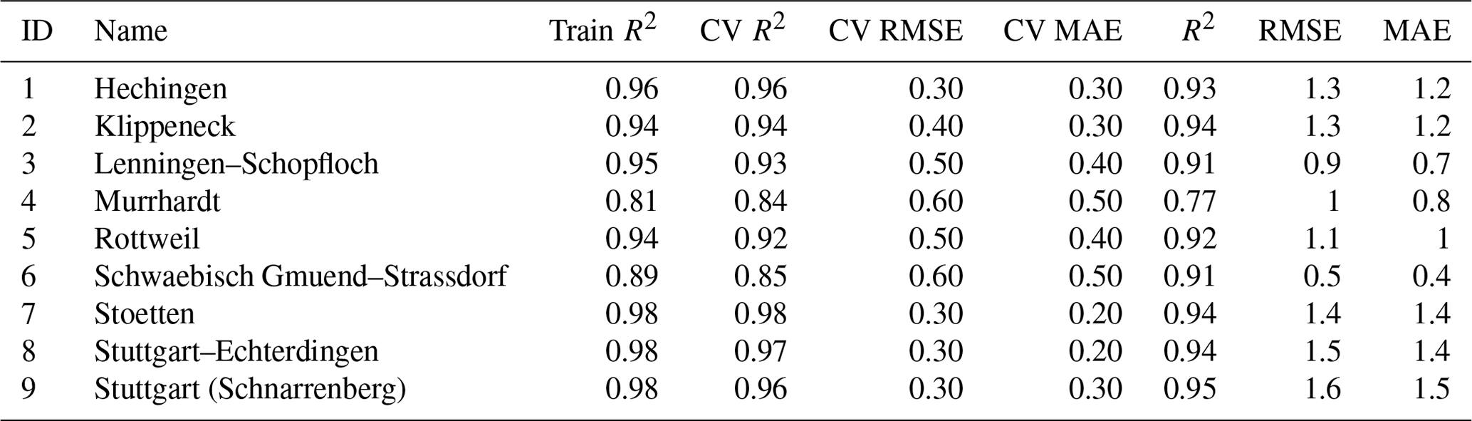
Following the analysis of the seven experimental models (Sect. 4.2), the recursive predictor selection method and stacking learning model (with LassoLarsCV, ARD, RandomForest, and bagging) were selected for the generation of the final ESD models. The models were trained on the 1958–2010 data in a CV setting and evaluated on the retained data in the 2011–2020 period. R2, RMSE, and MAE were used as performance metrics for the CV setting and the final evaluation (Tables 3 and 4). The models' performance was good overall but varied notably between different stations. The prediction skill estimates were higher for temperature than for precipitation. For temperature (Table 4), the explained variance estimates (“Fit R2”) are in the range of 0.81–0.98 (μ=0.94), and CV R2 values are in the range of 0.84 to 0.98 (μ=0.93), whereas for precipitation (Table 3), the explained variance estimates are in the range of 0.58–0.84 (μ=0.71), and CV R2 values are in the range of 0.54–0.72 (0.65). The accuracy measures display a similar discrepancy with CV RMSE of 0.3–0.6 ∘C (μ=0.42 ∘C) and CV MAE of 0.2–0.50 ∘C (μ=0.34 ∘C) for temperature, as well as CV RMSE of 20–24 mm per month (μ=21 mm per month) and CV MAE of 14–18 mm per month (μ=16 mm per month) for precipitation.
Table 3Model performance metrics (i.e., R2, RMSE, and MAE) for all the precipitation stations. The final ESD models were trained in a CV setting on datasets from 1958–2010 and evaluated on independent, retained data from 2011–2020.
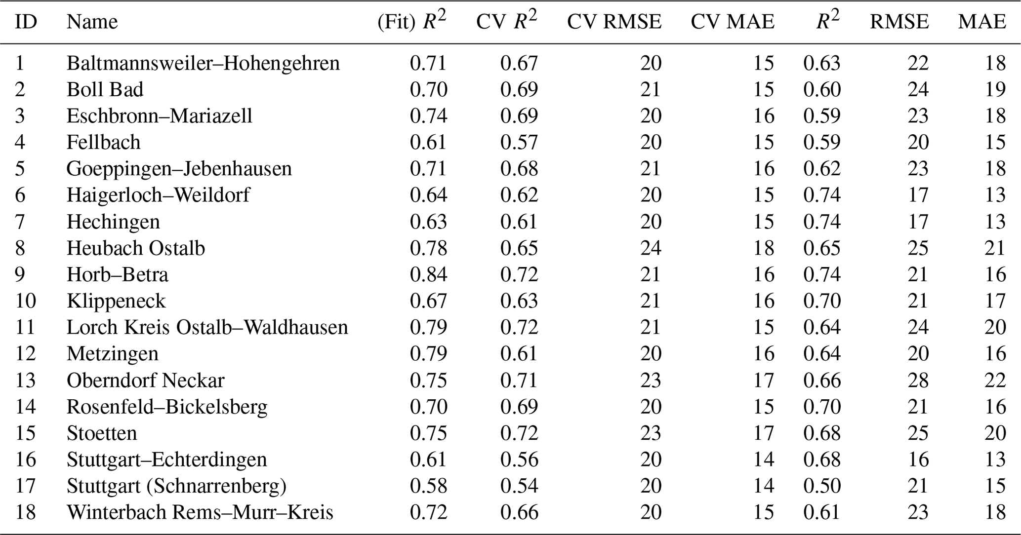
Table 4Model performance metrics (i.e., R2, RMSE, and MAE) for all the temperature stations. The final ESD models were trained in a CV setting on datasets from 1958–2010 and evaluated on independent, retained data from 2011–2020.
The final model evaluation using independent, retained data from 2011–2020 yielded R2 values of up to 0.95 as well as average RMSE and MAE of ∼1.0 ∘C for temperature and R2 values of up to 0.74, average RMSE of 22 mm per month, and MAE of 17 mm per month for precipitation. The discrepancy in temperature and precipitation model performance is unsurprising, since the thermodynamics and atmospheric dynamics controlling precipitation variability are more difficult to represent (e.g., Shepherd, 2014). Regardless, the overall performance speaks in favor of applying the study's approach to downscale midlatitude climate in complex terrain. Moreover, the models' similar performance during CV and the final evaluation indicates that the models were not overfitted and that the predictand–predictor relationships hold outside the observed period. Finally, it is worth noting that the stacking regressor performed better than the individual base models, even when all the potential regressors of the initial experiments (Sect. 4.2) were stacked into a meta-regressor. Such improvements demonstrate the advantage of the ease of experimentation through a package like pyESD.
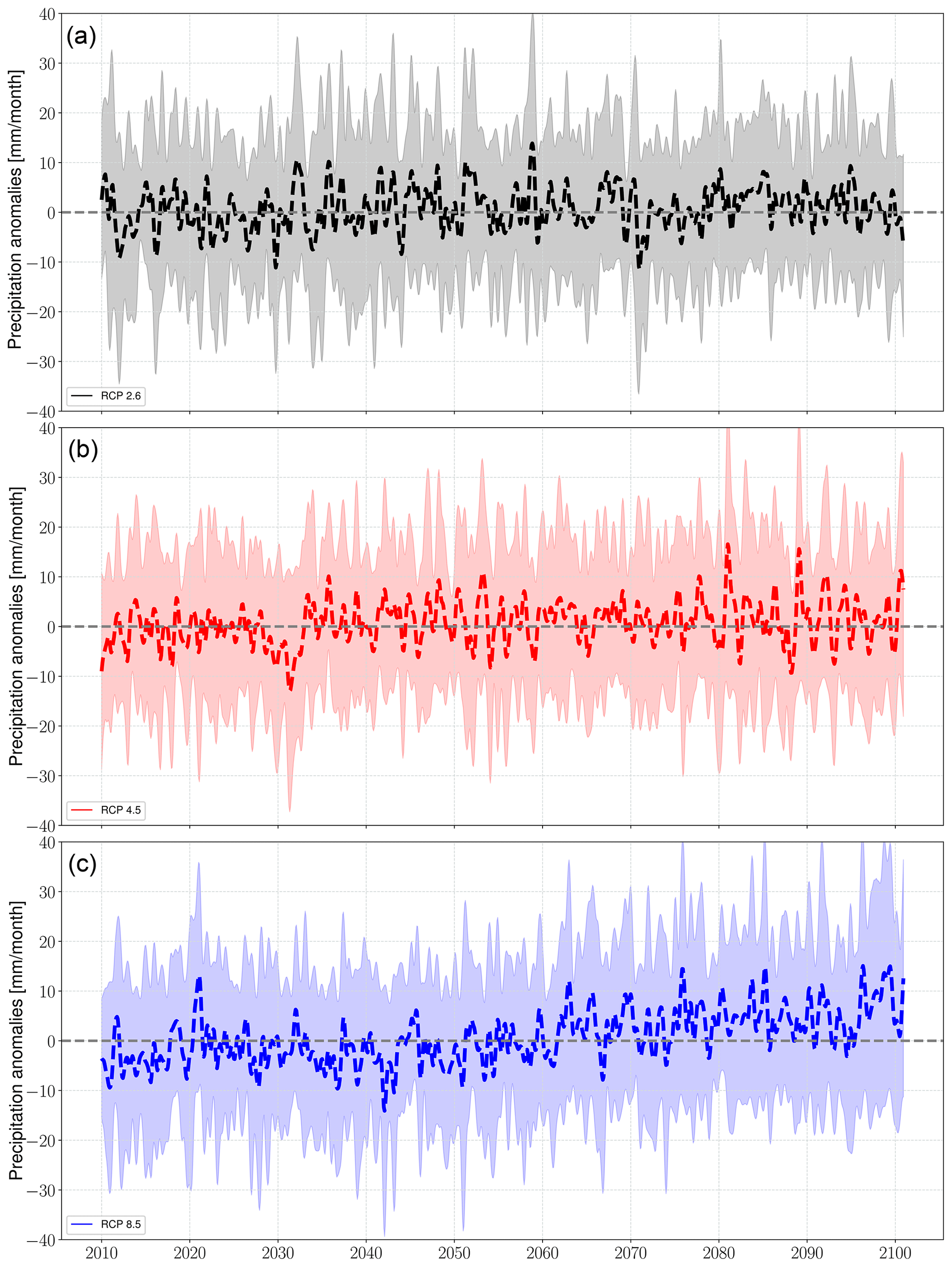
Figure 7Predicted regional annual means of precipitation in response to (a) RCP2.6 (black), (b) RCP4.5 (red), and (c) RCP8.5 (blue). The solid lines represent the values averaged over all stations, and the shaded boundaries indicate the corresponding variability range (1 standard deviation). The time series are smoothed with a 1-year moving average with a centered mean.
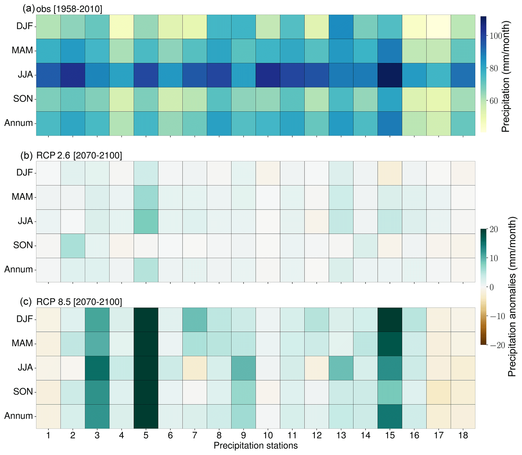
Figure 8(a) Observed precipitation (1958–2100) as well as seasonal (i.e., spring – MAM, summer – JJA, autumn – SON, and winter – DJF) and annual end-of-century (30-year) precipitation climatologies as a result of RCP2.6 (b) and RCP8.5 (c) forcing. Brown (green) indicates a decrease (increase) in precipitation relative to the observed means (1958–2010).
We visualize a prediction example (Fig. 6) to (a) provide a less abstract presentation of these results and (b) demonstrate the type of figure generated by the plotting utility functions in the pyESD.plot module. The figure depicts the predictions generated by the final ESD model for the Hechingen station, a station that records precipitation and temperature (station ID 7 and 1, respectively). The observed and predicted values for 2011–2020 are highly correlated, with PCCs of 0.85 (Fig. 6a) for precipitation and 0.97 (Fig. 6b) for temperature. The time series comparisons also demonstrate the models' abilities to predict the variability of the observed values in both the training and testing period (Fig. 6a and b). Prior to this study, PP-ESD models had not been directly applied to the weather stations in the catchment. However, our models are among the best performing for temperature and precipitation when we compare them to models from other studies across Europe (e.g., Gutiérrez et al., 2019; Hertig et al., 2019; Schmidli et al., 2007). For instance, Gutiérrez et al. (2019) performed an intercomparison of statistical downscaling model performance for 86 stations across Europe using the MOS, PP, and WG methods. The Spearman correlation of the downscaled and observed values yielded R values in the range of ∼0.0–0.7 (with many stations ≤0.5) for precipitation and 0.3–0.95 for temperature. These comparisons also underline the suitability of the pyESD methods for downscaling climate information even in complex mountainous regions.
4.4 Prediction of local responses to 21st century climate change
The predictions of local precipitation and temperature responses to 21st century climate change were generated by coupling the final ESD models to MPI-ESM simulations forced with greenhouse gas concentration scenarios RCP2.6, RCP4.5, and RCP8.5 (Sect. 3.2.3). The results are presented as deviations from the monthly long-term means of the training period (1958–2010) and referred to as “anomalies” hereafter. The annual mean anomaly time series were computed with a 1-year moving average with a centered mean (Figs. 7 and 9).
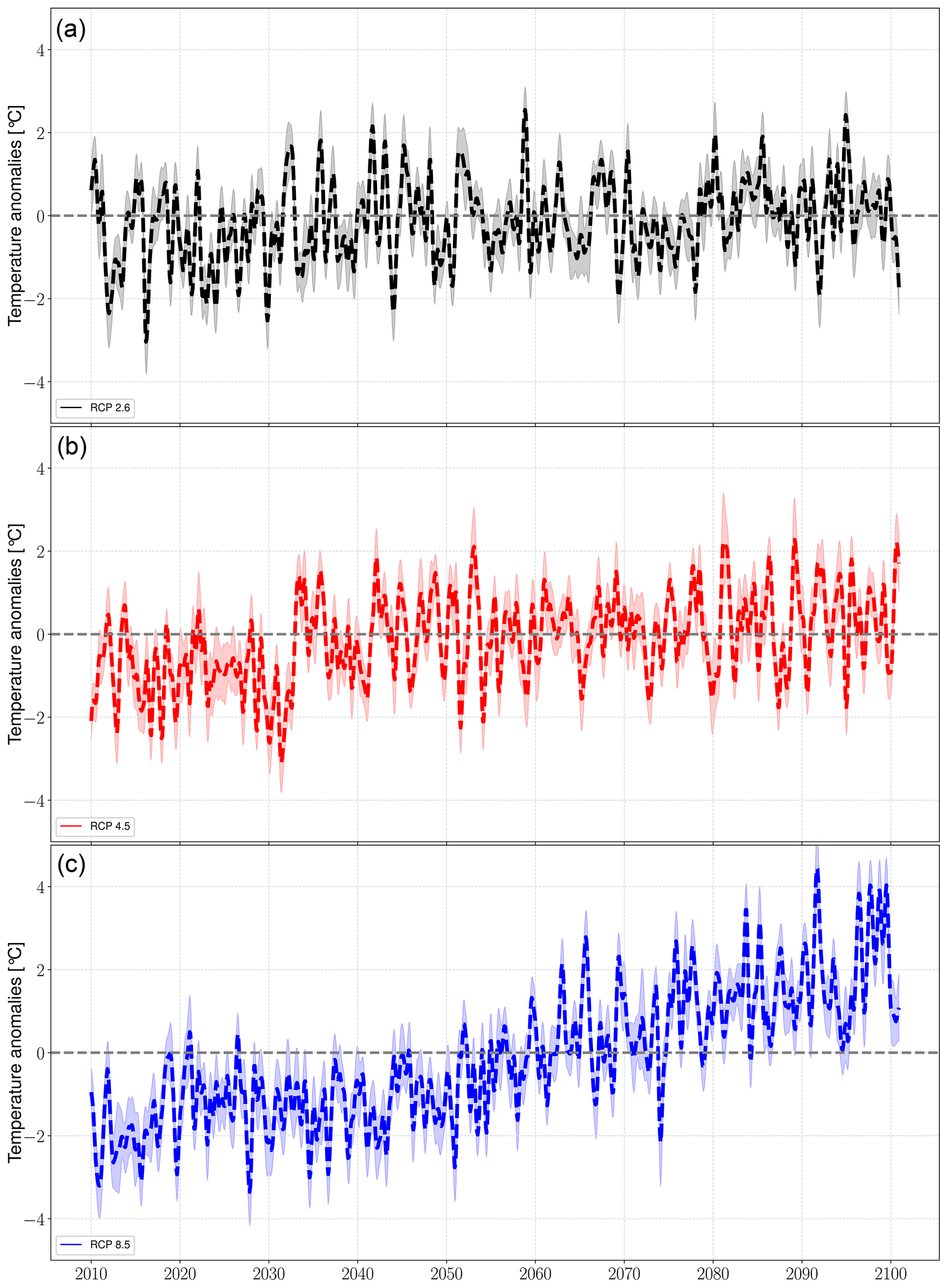
Figure 9Predicted regional annual means of the temperature in response to (a) RCP2.6 (black), (b) RCP4.5 (red), and (c) RCP8.5 (blue). The solid lines represent the values averaged over all stations, and the shaded boundaries indicate the corresponding variability range (1 standard deviation). The time series are smoothed with a 1-year moving average with a centered mean.
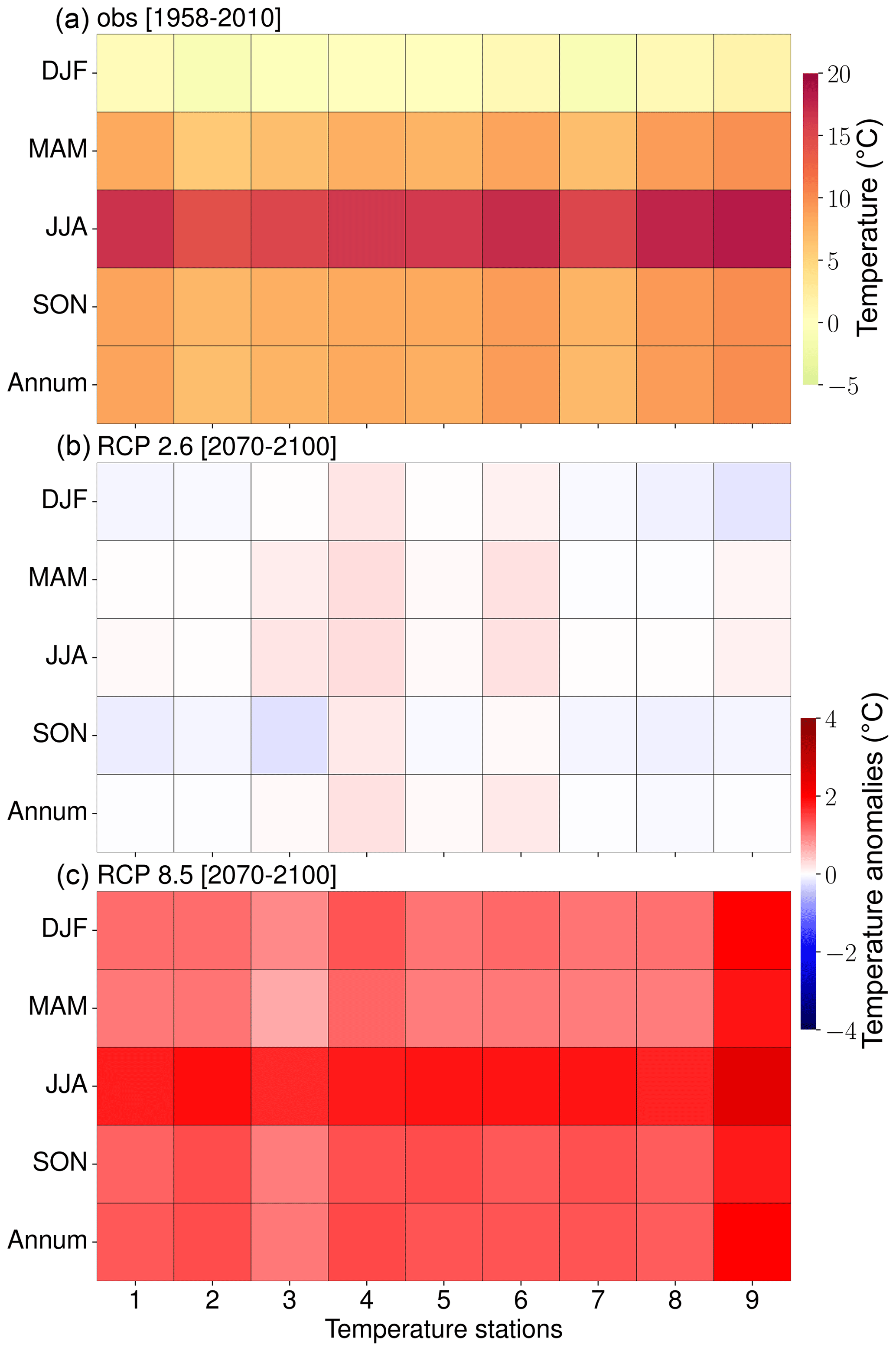
Figure 10(a) Observed temperature (1958–2100) as well as seasonal (i.e., spring – MAM, summer – JJA, autumn – SON, and winter – DJF) and annual end-of-century (30-year) temperature climatologies as a result of RCP2.6 (b) and RCP8.5 (c) forcing. Blue (red) indicates a decrease (increase) in temperature relative to the observed means (1958–2010).
The precipitation predictions (Fig. 7) for RCP8.5 (RCP4.5) show a strong (weak) positive trend towards the end of the century. This trend is even more pronounced for the predicted temperatures (Fig. 9) in the catchment. The predicted precipitation changes vary greatly between weather stations. Furthermore, the RCPs change the magnitude but not the pattern of the predictions for each station. For instance, stations that show an increase (decrease) in precipitation for the RCP2.6 predict a greater increase (decrease) in response to RCP4.5 and RCP8.5. The annual and seasonal 30-year end-of-century climatologies show an overall increase in precipitation in response to both RCP2.6 and RCP4.5 (Fig. 8) for most of the stations. The annual end-of-century climatologies deviate from the present day (1958–2010) by ca. −5 to 20 mm per month for RCP8.5 and ca. ≤5 mm per month for RCP2.6. Overall, the ESD models predict a precipitation increase of ca. 10 %–20 % until the end of the century. Furthermore, the seasonal climatologies reveal a shift of maximum precipitation away from the summer season for some stations. Such shifts in seasonality and an overall decrease in summer precipitation have previously been predicted (e.g., Gobiet et al., 2014; Paparrizos et al., 2017; Feldmann et al., 2013). Prior to this study, no ESD–GCM-based predictions of the 21st century precipitation changes had been developed for the weather stations of the catchment. However, the models' predictions of the precipitation response to higher greenhouse gas concentration scenarios are comparable to coarser predictions by other studies using RCMs or ESD models (Feldmann et al., 2013; Kunstmann et al., 2004; Paparrizos et al., 2017; Lau et al., 2013). The precipitation predictions generated in this case study can be used further for climate impact assessments, such as assessments of the probability of flooding and drought across the hydrological catchment. The projected shifts in seasonality across the catchment represents potentially valuable information for agricultural planning.
The predicted temperature anomalies (Fig. 9) reveal a strong (weak) positive trend for RCP8.5 (RCP4.5). The end-of-century climatologies reveal only moderate warming of ca. −0.5 to 1 ∘C for RCP2.6 and significant warming (ca. 2–4 ∘C) for all seasons in response to RCP8.5 (Fig. 10). More specifically, the investigated region is predicted to experience the most warming (≥3 ∘C) in the summer season. There are few differences in predicted warming between the stations of the catchment. Generally, the estimated magnitude of warming towards the end of the century is in agreement with the IPCC report (IPCC, 2021) and other downscaled estimates (e.g., Kunstmann et al., 2004; Gutiérrez et al., 2019). The predicted warming would likely implicate societal and ecological systems and stresses the need for efficient adaptation and mitigation strategies.
The case study highlights the efficiency and robustness of the downscaling steps implemented in the pyESD package. However, as noted in previous sections, the accuracy of the predictions generated by a GCM–ESD model coupling relies on the predictors being adequately represented by the GCMs. KS tests were performed to evaluate this for the temporal overlap (1979–2000) between the ERA5 reanalysis product and the MPI-ESM GCM output (Sect. 3.2.3). Results from these tests show significant differences in the distribution of ERA5 and MPI-ESM when the raw monthly time series are considered, thus violating the assumptions of the PP-ESD approach. However, this issue does not persist for monthly standardized anomalies of precipitation and temperature (Fig. 11). Previous studies yielded similar results when using seasonal standardizers (Bedia et al., 2020) and principal component transformations (Benestad et al., 2015a), both of which are included in the pyESD package.
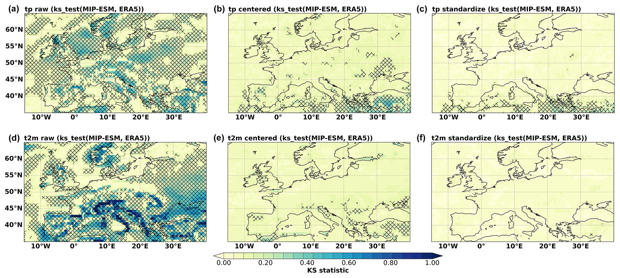
Figure 11The KS two-sided statistical testing score maps the ERA5 reanalysis product and MPI-ESM GCM output for precipitation (a–c) and temperature (d–f). The KS test was applied to raw values, anomalies (centered with zero means), and standardized anomalies with unit variance values (columns from left to right, respectively). The grid boxes with black cross stippling represent low p values (p<0.05), suggesting statistically significant differences in distribution between the ERA5 and MPI-ESM time series.
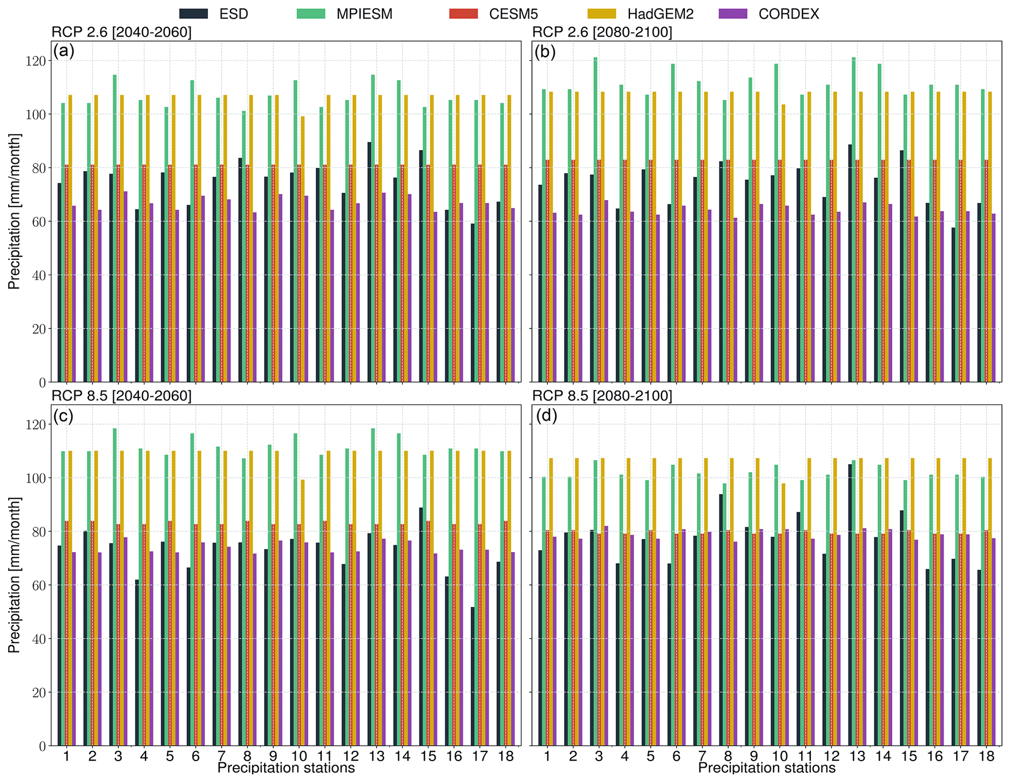
Figure 12Comparison of 20-year annual precipitation climatologies predicted by the ESD models of this study (black), GCMs (i.e., MPI-ESM in green, CESM5 in red, HadGEM2 in gold), and RCMs (i.e., and CORDEX in purple) for RCP2.6 (a, b) and RCP8.5 (c, d).
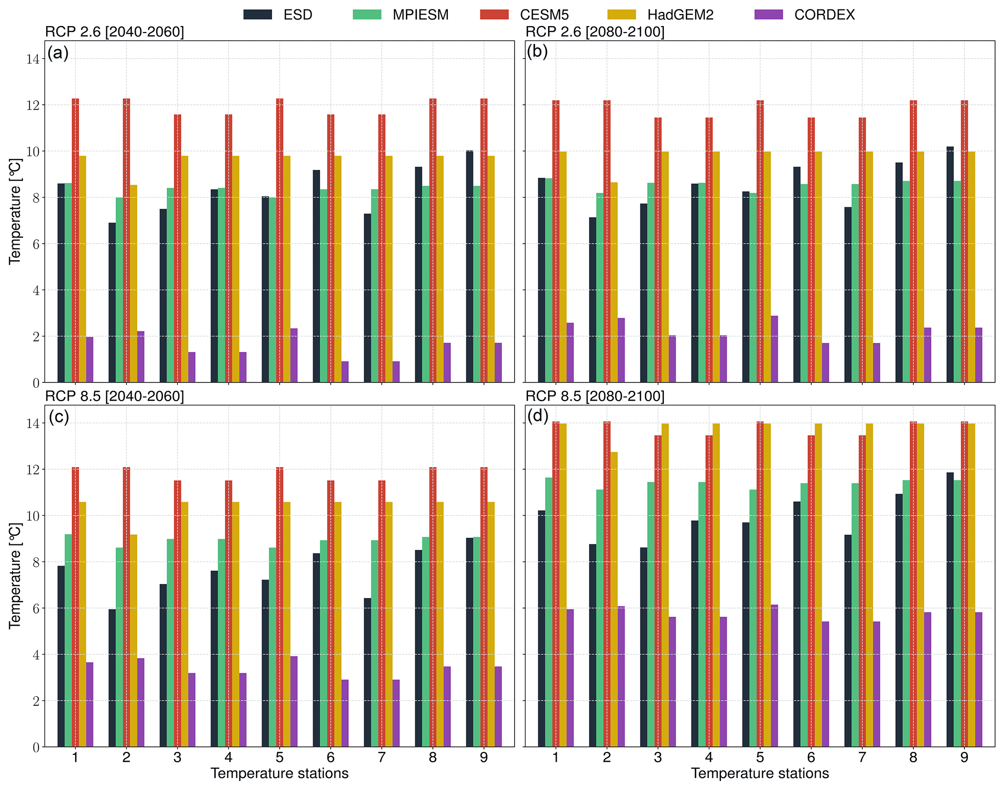
Figure 13Comparison of 20-year annual temperature climatologies predicted by the ESD models of this study (black), GCMs (i.e., MPI-ESM in green, CESM5 in red, HadGEM2 in gold), and RCMs (i.e., and CORDEX in purple) for RCP2.6 (a, b) and RCP8.5 (c, d).
4.5 Comparison of GCM and ESD-based predictions
A comparison of the ESD-generated annual 20-year climatologies for the mid-century (2040–2060) and the end of the century (2080–2100) to the model output of GCMs and RCMs (i.e., EURO-CORDEX) reveals several differences. The GCMs (MPI-ESM and HadGEM2) predict ∼20 mm per month (∼30 %) higher precipitation rates than the ESD models and RCMs. The ESD-based precipitation predictions of this study are closest to the RCM estimates but mm per month higher in magnitude for most of the stations (Fig. 12). The closeness of the ESD-based and RCM-based estimates underlines the added value of our ESD approach for downscaling precipitation. However, there are significant (∼4 ∘C) differences between the ESD-based and RCM-based temperature estimates (Fig. 13). The ESD-based temperature predictions were higher than those of the RCM but lower than those of the GCM. Both the RCM and ESD models used boundary conditions from the same GCM (MPI-ESM). The RCM reduced the GCM temperatures by more (∼8 ∘C) than the ESD models (∼4 ∘C or less). This may be a reflection of both (a) the selection of GCM near-surface temperatures as predictors in the ESD models and (b) the shrinking of regression coefficients when the ESD transfer functions are determined.
Contemporary climate change and its impacts increase the demand for high-resolution, regional- and local-scale predictions. These can be generated in a most cost-effective way through the application of the PP-ESD (perfect prognosis empirical-statistical downscaling) approach. The pyESD Python package we introduce here is a well-developed tool and modeling framework for applying and experimenting with PP-ESD for any climate variable (e.g., precipitation, wind speed, and temperature). The package complements existing tools through the following key specialties and strengths.
-
The package is well-structured and designed in OOP style that treats the weather stations as objects with many functionality attributes that cover all the PP-ESD modeling routines. As a result, all modeling steps can be executed on the initialized station objects with a few lines of code.
-
The package is designed in a way that knowing its API (Application Programming Interface), which is introduced in the package's extensive documentation, is sufficient to implement all downscaling steps. In other words, no advanced knowledge of Python (or programming) is required to use the package for research purposes. On the other hand, the package's design is modular and flexible enough to allow advanced users to build on it or adjust it to their needs.
-
The package implements different predictor selection techniques (i.e., recursive, tree-based, and sequential) that can be manually selected and experimented with. The package allows the user to include a variety of predictors, ranging from regional near-surface temperatures to synoptic-scale teleconnection patterns. The package features many transformation techniques such as MonthlyStandardizer and PCAScalling that can be used to reduce biases towards specific predictors.
-
The package includes a variety of machine learning techniques with different underlying principles and theorems. The package also features many ensemble models (Sect. 2.3), cross-validation schemes, and hyperparameter optimization techniques that can easily be experimented with in a few lines of code.
-
The package's core modules are accompanied by utility functions for data preprocessing, post-processing, and serialization to save computational resources, as well as visualization tools and ESD-relevant statistical methods like EOF analysis, correlation, and distribution similarity tests.
We demonstrated some of the package's functionalities by developing and applying ESD models to generate precipitation and temperature predictions for a sub-hydrological catchment in complex mountainous terrain in southwestern Germany. The models were evaluated with different metrics and were found to perform well (e.g., R2≥0.7 for precipitation and R2≥0.9 for temperature). In order to ensure the reproducibility of the results and allow easy practical entry for potential users, the application example uses publicly available datasets, and all the scripts used for this study are made available.
Despite the promising results of the illustrative case study, the reader is informed of the following important limitations: generally, the PP-ESD approach to predictions relies on the assumption that the empirical relationships between predictor and predictand remain valid through time. While statistical downscaling models have successfully been used for the past climate of the pre-industrial era (Reichert et al., 1999) and Last Glacial Maximum (Vrac et al., 2007), the merit of this assumption must be evaluated on a case-by-case basis. For example, geographical boundary conditions that affect the local climate, such as topography or vegetation cover, are only implicitly considered in the empirical transfer functions. The empirical relationship between predictors and predictands may break down if these boundary conditions change significantly (e.g., Mutz and Aschauer, 2022). Furthermore, the performance of PP-ESD models also depends on the accuracy of the GCMs they are coupled to. In our case study, the developed ESD models were coupled to a single, albeit well-established, GCM (MPI-ESM). However, we generally recommend the use of GCM ensembles to prevent biases towards a specific GCM.
The current version of the package includes all functions needed to develop, evaluate, and apply station-based ESD models and generate predictions of local-scale climate change. Nevertheless, the package remains under active development to expand upon its functionality. Planned improvements include an extension of functions to make pyESD suitable for downscaling gridded datasets or satellite observations. The grid-based analysis would contribute to the design of spatial downscaling models (e.g., Chen et al., 2012; Jia et al., 2011). Moreover, we intend to expand the selection of machine learning techniques by including deep learning models that have been proven useful in downscaling (e.g., Baño-Medina et al., 2020; Quesada-Chacón et al., 2022). Finally, we intend to build a graphical, web-based interface to make the package more accessible and easy to use for researchers, students, and people outside the scientific community.
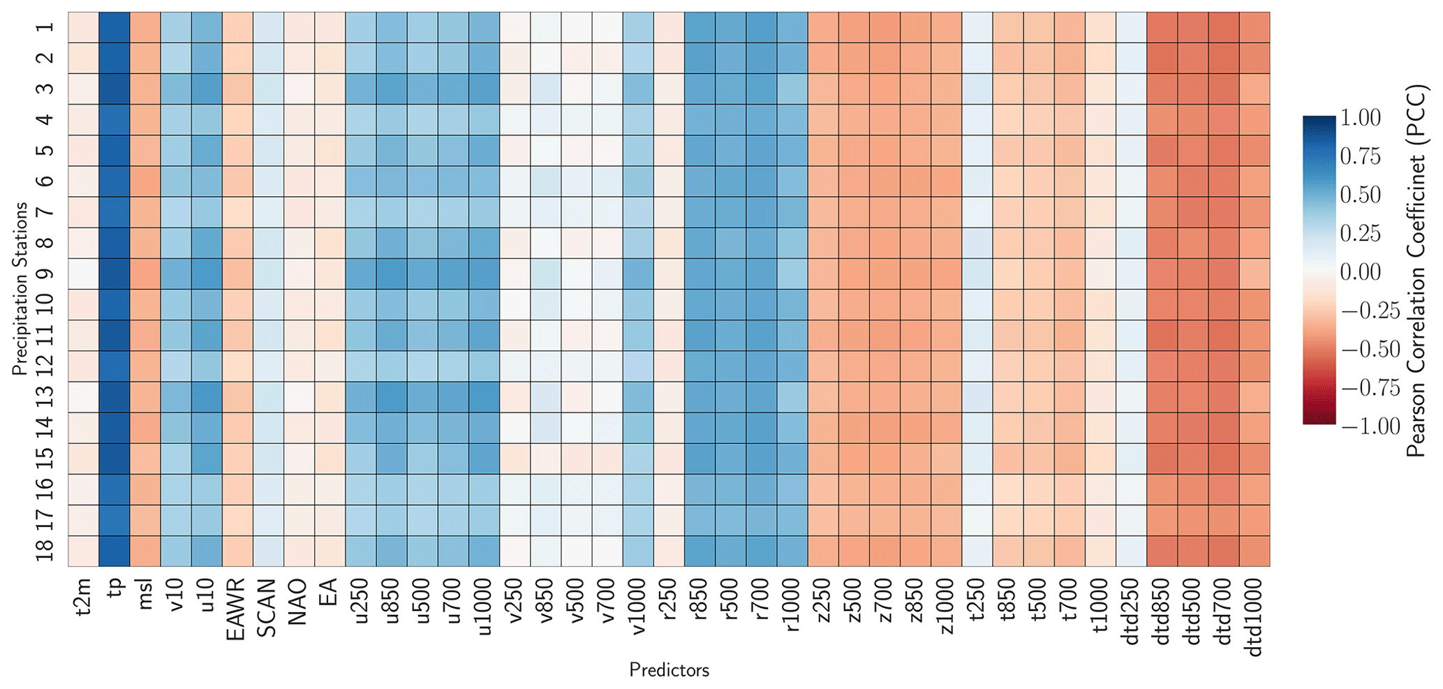
Figure A1Correlation between the precipitation predictand and the potential predictors listed in Table 2, expressed as PCCs.
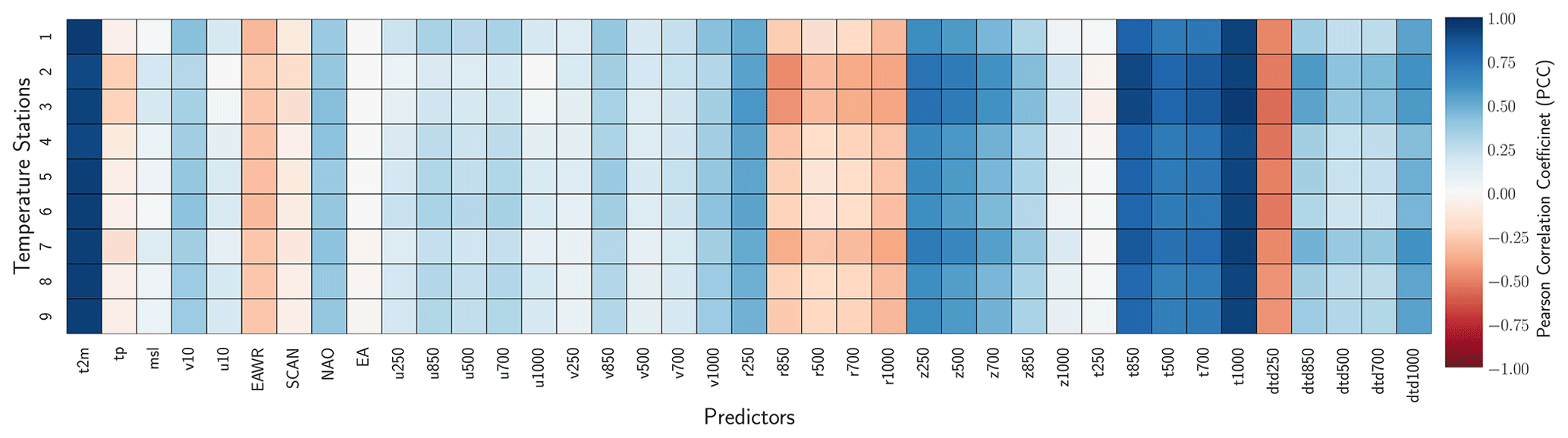
Figure A2Correlation between the temperature predictand and the potential predictors listed in Table 2, expressed as PCCs.
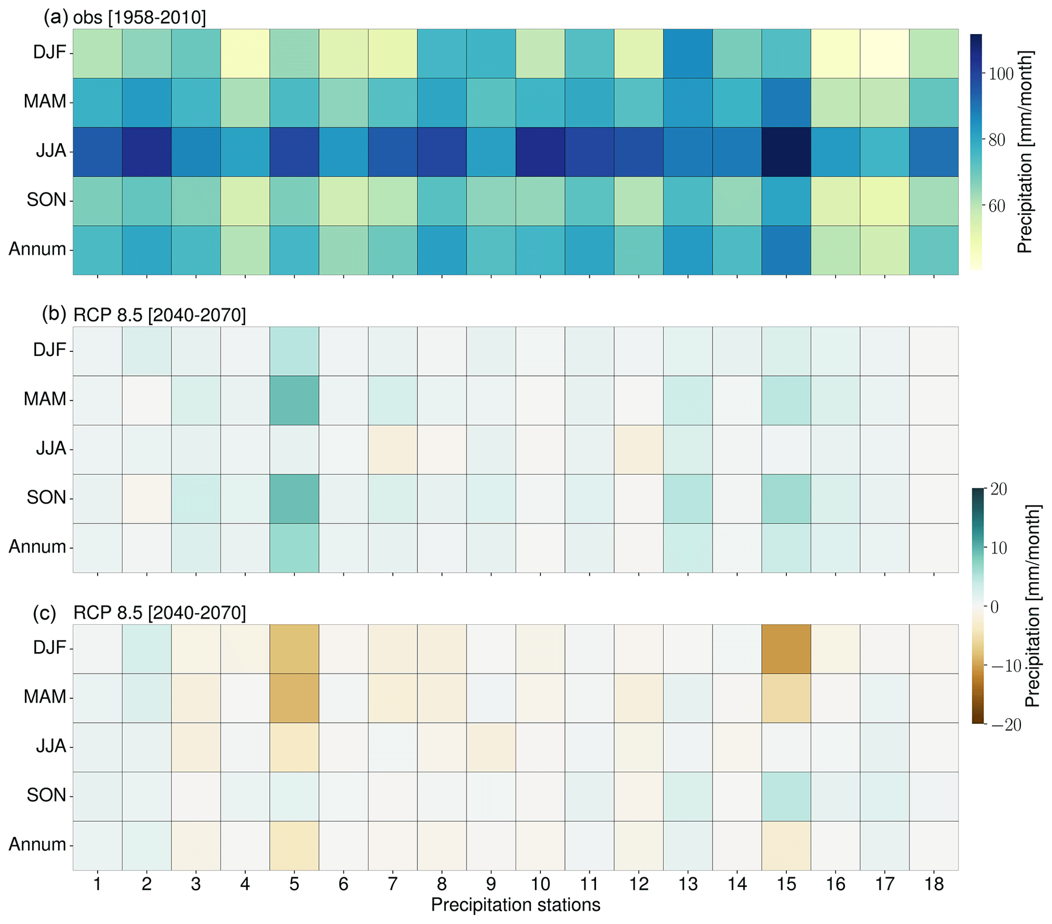
Figure A3(a) Observed precipitation (1958–2010) as well as seasonal (i.e., spring – MAM, summer – JJA, autumn – SON, and winter – DJF) and annual mid-century (30-year) precipitation climatologies as a result of RCP2.6 (b) and RCP8.5 (c) forcing. Brown (green) indicates a decrease (increase) in precipitation relative to the observed means (1958–2010).
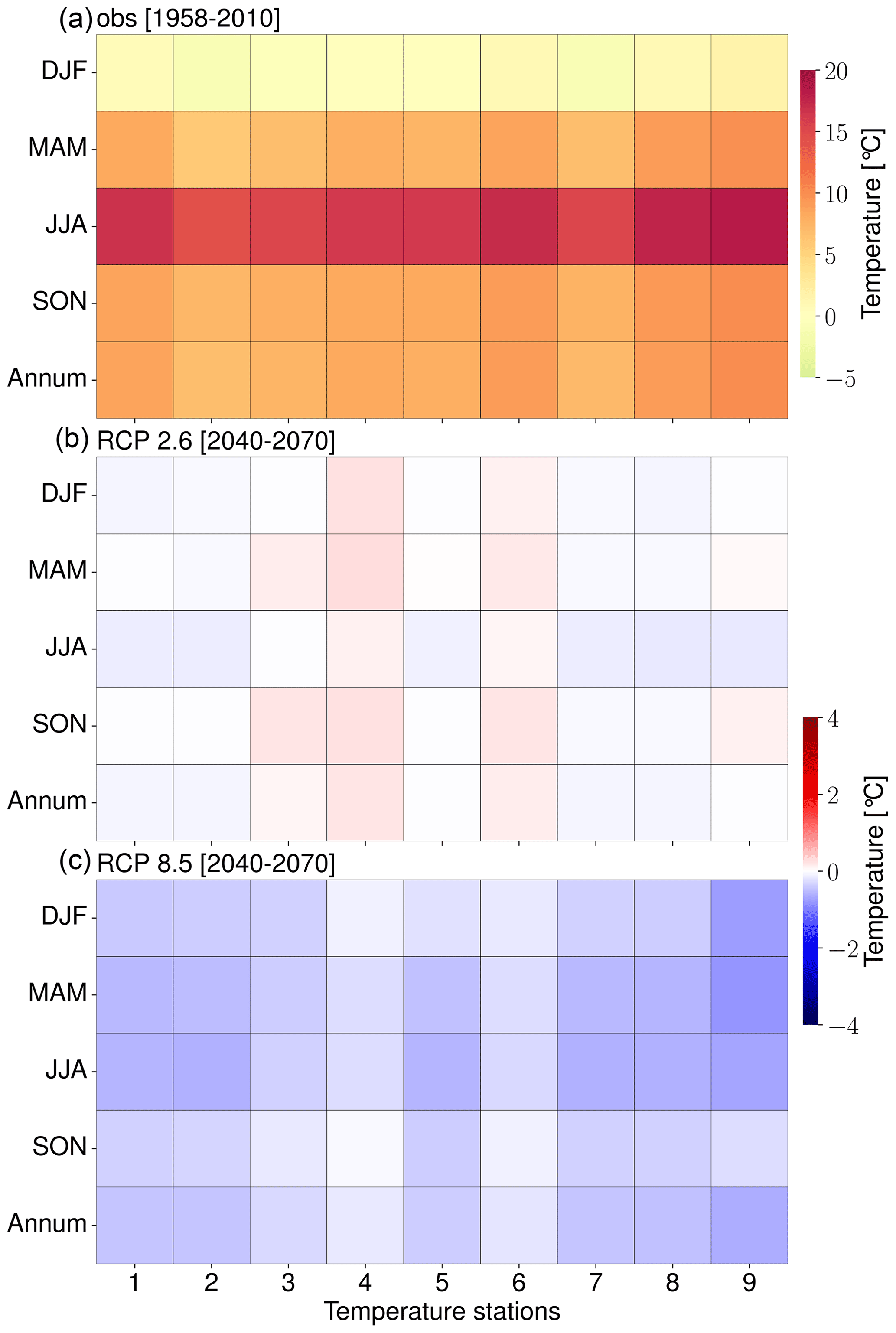
Figure A4Observed temperature (1958–2010) as well as seasonal (i.e., spring – MAM, summer – JJA, autumn – SON, and winter – DJF) and annual mid-century (30-year) temperature climatologies as a result of RCP2.6 (b) and RCP8.5 (c) forcing. Blue (red) indicates a decrease (increase) in temperature relative to the observed means (1958–2010).
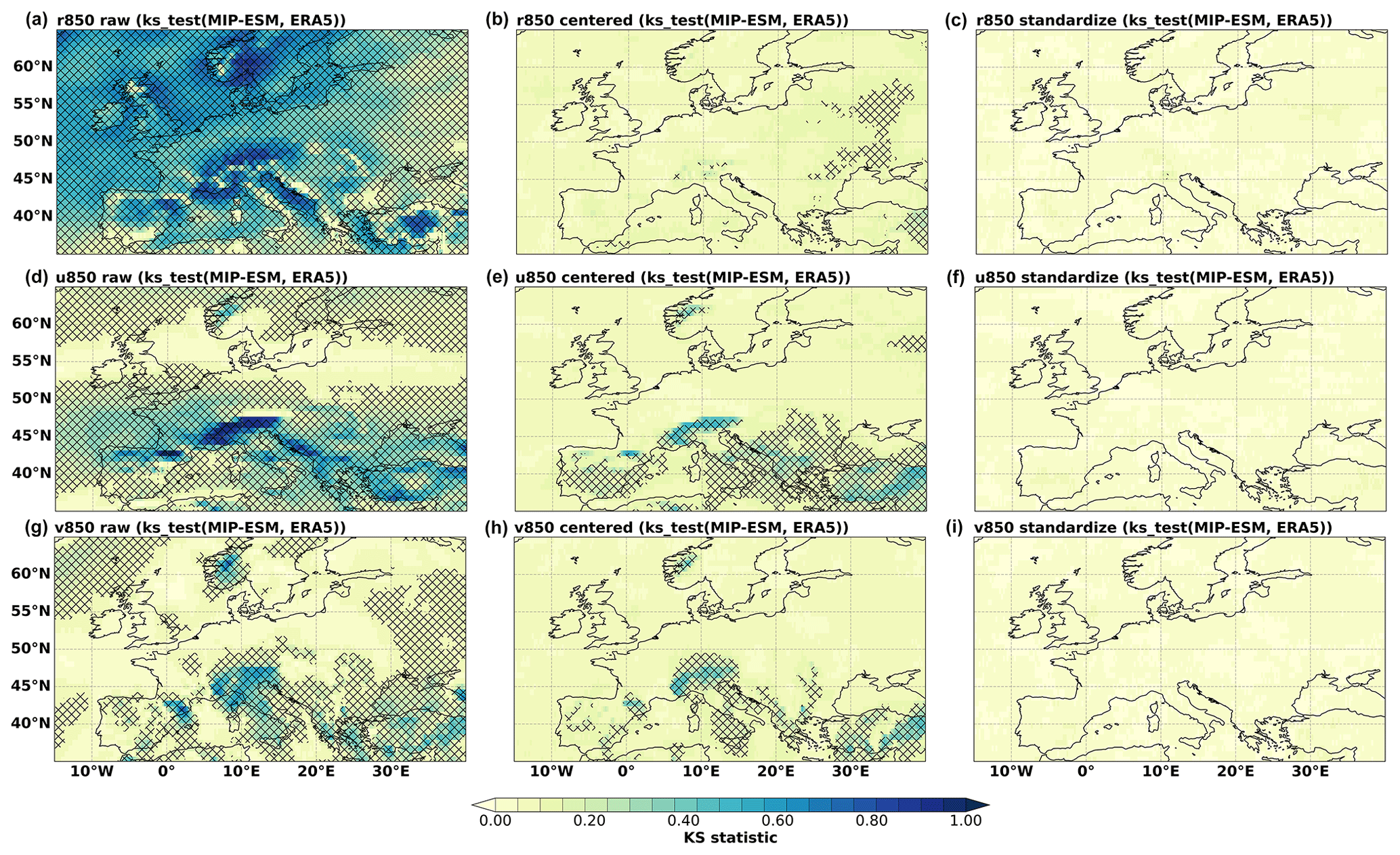
Figure A5The KS two-sided statistical testing score maps the ERA5 reanalysis product and MPI-ESM GCM output for relative humidity (a–c), zonal wind velocity (d–f), and meridional wind velocity (g–i) at 850 hPa. The KS test was applied to raw values, anomalies (centered with zero means), and standardized anomalies with unit variance values (columns from left to right, respectively). The grid boxes with black cross stippling represent low p values (p<0.05), suggesting statistically significant differences in distribution between the ERA5 and MPI-ESM time series.
The study's illustrative case study relies on publicly available datasets. More specifically, the precipitation and temperature datasets are accessible through the Climate Data Centre of the DWD (Deutscher Wetterdienst, version V21.3). The subcatchment datasets used in this study are interactively available through https://cdc.dwd.de/portal/shortlink/425267fe-e4fd-4fff-9969-14c7d3aa25de (Deutscher Wetterdienst, 2023) and https://cdc.dwd.de/portal/shortlink/da6f555d-d6f6-426a-a8ba-b96683c76ea9 (last access: 30 October 2023) for precipitation and temperature stations, respectively. The ERA5 reanalysis datasets can also be downloaded through the Copernicus Climate Data Store (CDS) at https://doi.org/10.24381/cds.6860a573 (Hersbach et al., 2023) for pressure level and https://doi.org/10.24381/cds.68d2bb30 (Muñoz Sabater, 2019) for surface-level variables. However, the processed weather stations and the serialized pickle files of the regional means of the predictors for all the stations are provided as part of the supporting material (https://doi.org/10.5281/zenodo.7767681, Boateng and Mutz, 2023). The MPI-ESM GCM datasets used as simulated predictors can also be downloaded from the CDS by selecting MPI-ESM-LR as the model for the AMIP as well as the RCP2.6, 4.5, and 8.5 experiments: see https://doi.org/10.24381/cds.3b4b5bc9 (Copernicus Climate Change Service, Climate Data Store, 2018a) for pressure-level variables and https://doi.org/10.24381/cds.9d44a987 (Copernicus Climate Change Service, Climate Data Store, 2018b) for surface variables. Moreover, the station-based downscaling estimates of future climate scenarios for all the stations are also included in the supporting material (https://doi.org/10.5281/zenodo.7767681, Boateng and Mutz, 2023).
The pyESD (version 1.0.1) software, including the documentation website source files, is available through many platforms, including the following.
-
GitHub: https://github.com/Dan-Boat/PyESD (last access: 30 October 2023)
-
Python package index (PyPI): https://pypi.org/project/PyESD/ (last access: 30 October 2023)
-
Zenodo (v1.0.1 release):
https://doi.org/10.5281/zenodo.7767629 (Boateng, 2023)
Developer: Daniel Boateng, University of Tübingen
Hardware requirements: general-purpose computer
Programming language: Python (version 3.7 or later)
The installation of the package and its required dependencies are highlighted on the documentation website: https://dan-boat.github.io/PyESD/ (last access: 30 October 2023). The usage of the package and its functionalities are also presented in the documentation. The control scripts of the study's illustrative case study are also provided as part of the supporting material (https://doi.org/10.5281/zenodo.7767681, Boateng and Mutz, 2023) and also presented in the example section of the documentation.
DB: pyESD software and documentation website development, conceptualization, modeling, data analysis, visualization, and writing of the original paper. SGM: supervision, paper editing, and funding acquisition.
The contact author has declared that neither of the authors has any competing interests.
Publisher's note: Copernicus Publications remains neutral with regard to jurisdictional claims made in the text, published maps, institutional affiliations, or any other geographical representation in this paper. While Copernicus Publications makes every effort to include appropriate place names, the final responsibility lies with the authors.
This study was partially supported by the German Science Foundation (DFG) under grant nos. MU4188/3-1 and MU4188/1-1, awarded to Sebastian G. Mutz. We acknowledge the World Climate Research Programme, which, through its Working Group on Coupled Modelling, coordinated and promoted CMIP5. We thank the climate modeling groups for producing and making available their model output, the Earth System Grid Federation (ESGF) for archiving the data and providing access, and the multiple funding agencies who support CMIP5 and ESGF. We also thank the European Centre for Medium-Range Weather Forecasts for providing the ERA5 data product and the Deutsche Wetterdienst (DWD) for providing the weather station records. W We thank Charles Onyutha and the three anonymous reviewers for their constructive reviews.
This research has been supported by the Deutsche Forschungsgemeinschaft (grant nos. MU4188/3-1 and MU4188/1-1).
This open-access publication was funded by the University of Tübingen.
This paper was edited by Charles Onyutha and reviewed by three anonymous referees.
Anandhi, A., Srinivas, V. V., Nanjundiah, R. S., and Nagesh Kumar, D.: Downscaling precipitation to river basin in India for IPCC SRES scenarios using support vector machine, Int. J. Climatol., 28, 401–420, https://doi.org/10.1002/joc.1529, 2008.
Arlot, S. and Celisse, A.: A survey of cross-validation procedures for model selection, Stat. Surv., 4, 40–79, https://doi.org/10.1214/09-SS054, 2010.
Balasundaram, S. and Tanveer, M.: On Lagrangian twin support vector regression, Neural Comput. Appl., 22, 257–267, 2013.
Baño-Medina, J., Manzanas, R., and Gutiérrez, J. M.: Configuration and intercomparison of deep learning neural models for statistical downscaling, Geosci. Model Dev., 13, 2109–2124, https://doi.org/10.5194/gmd-13-2109-2020, 2020.
Bárdossy, A.: Atmospheric circulation pattern classification for South-West Germany using hydrological variables, Phys. Chem. Earth Parts A/B/C, 35, 498–506, https://doi.org/10.1016/j.pce.2010.02.007, 2010.
Barnston, A. G. and Livezey, R. E.: Classification, Seasonality and Persistence of Low-Frequency Atmospheric Circulation Patterns, Mon. Weather Rev., 115, 1083–1126, https://doi.org/10.1175/1520-0493(1987)115<1083:CSAPOL>2.0.CO;2, 1987.
Bedia, J., Baño-Medina, J., Legasa, M. N., Iturbide, M., Manzanas, R., Herrera, S., Casanueva, A., San-Martín, D., Cofiño, A. S., and Gutiérrez, J. M.: Statistical downscaling with the downscaleR package (v3.1.0): contribution to the VALUE intercomparison experiment, Geosci. Model Dev., 13, 1711–1735, https://doi.org/10.5194/gmd-13-1711-2020, 2020.
Bell, B., Hersbach, H., Simmons, A., Berrisford, P., Dahlgren, P., Horányi, A., Muñoz-Sabater, J., Nicolas, J., Radu, R., Schepers, D., Soci, C., Villaume, S., Bidlot, J.-R., Haimberger, L., Woollen, J., Buontempo, C., and Thépaut, J.-N.: The ERA5 global reanalysis: Preliminary extension to 1950, Q. J. Roy. Meteor. Soc., 147, 4186–4227, https://doi.org/10.1002/qj.4174, 2021.
Benestad, R. E., Chen, D., Mezghani, A., Fan, L., and Parding, K.: On using principal components to represent stations in empirical–statistical downscaling, Tellus A, 67, 28326, https://doi.org/10.3402/tellusa.v67.28326, 2015a.
Benestad, R. E., Mezghani, A., and Parding M. K.: “esd” – The Empirical-Statistical Downscaling tool & its visualisation capabilities, Figshare, https://doi.org/10.6084/m9.figshare.1454425.v1, 2015b.
Bergmeir, C. and Benítez, J. M.: On the use of cross-validation for time series predictor evaluation, Inform. Sciences, 191, 192–213, https://doi.org/10.1016/j.ins.2011.12.028, 2012.
Bergstra, J. and Bengio, Y.: Random search for hyper-parameter optimization, J. Mach. Learn. Res., 13, 281–305, 2012.
Bergstra, J., Bardenet, R., Bengio, Y., and Kégl, B.: lgorithms for hyper-parameter optimization, in: Proceedings of the 24th International Conference on Neural Information Processing Systems, 2546–2554, 2011.
Bishop, C. M. and Nasrabadi, N. M.: Pattern recognition and machine learning, Springer, ISBN 978-1-4939-3843-8, 2006.
Boateng, D.: Dan-Boat/PyESD: PyESDv1.0.1 (v1.0.1), Zenodo [code], https://doi.org/10.5281/zenodo.7767629, 2023.
Boateng, D. and Mutz, S. G.: Supporting material for PyESDv1.0.1 An open-source Python framework for empirical-statistical downscaling of climate information, Zenodo [data set], https://doi.org/10.5281/zenodo.7767681, 2023.
Boateng, D., Mutz, S. G., Ballian, A., Meijers, M. J. M., Methner, K., Botsyun, S., Mulch, A., and Ehlers, T. A.: The effects of diachronous surface uplift of the European Alps on regional climate and the oxygen isotopic composition of precipitation, Earth Syst. Dynam. Discuss. [preprint], https://doi.org/10.5194/esd-2022-48, in review, 2022.
Boé, J., Terray, L., Martin, E., and Habets, F.: Projected changes in components of the hydrological cycle in French river basins during the 21st century, Water Resour. Res., 45, W08426, https://doi.org/10.1029/2008WR007437, 2009.
Bottou, L.: Stochastic gradient learning in neural networks, Proc. Neuro-Nımes, 91, https://leon.bottou.org/publications/pdf/nimes-1991.pdf (last access 30 October 2023), 1991.
Bourgault, P., Huard, D., Smith, T. J., Logan, T., Aoun, A., Lavoie, J., Dupuis, É., Rondeau-Genesse, G., Alegre, R., Barnes, C., Laperrière, A. B., Biner, S., Caron, D., Ehbrecht, C., Fyke, J., Keel, T., Labonté, M.-P., Lierhammer, L., Low, J.-F., Quinn, J., Roy, P., Squire, D., Stephens, A., Tanguy, M., and Whelan, C.: xclim: xarray-based climate data analytics, J. Open Source Softw., 8, 5415, https://doi.org/10.21105/joss.05415, 2023.
Brands, S., Gutiérrez, J. M., Herrera, S., and Cofiño, A. S.: On the Use of Reanalysis Data for Downscaling, J. Climate, 25, 2517–2526, https://doi.org/10.1175/JCLI-D-11-00251.1, 2012.
Breiman, L.: Bagging predictors, Mach. Learn., 24, 123–140, 1996a.
Breiman, L.: Stacked regressions, Mach. Learn., 24, 49–64, https://doi.org/10.1007/BF00117832, 1996b.
Breiman, L.: Random forests, Mach. Learn., 45, 5–32, 2001.
Chaudhuri, A. and Hu, W.: A fast algorithm for computing distance correlation, Comput. Stat. Data Anal., 135, 15–24, https://doi.org/10.1016/j.csda.2019.01.016, 2019.
Chen, J., Brissette, F. P., and Leconte, R.: Coupling statistical and dynamical methods for spatial downscaling of precipitation, Clim. Change, 114, 509–526, https://doi.org/10.1007/s10584-012-0452-2, 2012.
Chen, S.-T., Yu, P.-S., and Tang, Y.-H.: Statistical downscaling of daily precipitation using support vector machines and multivariate analysis, J. Hydrol., 385, 13–22, https://doi.org/10.1016/j.jhydrol.2010.01.021, 2010.
Chen, T. and Guestrin, C.: XGBoost: A Scalable Tree Boosting System, in: Proceedings of the 22nd ACM SIGKDD International Conference on Knowledge Discovery and Data Mining, KDD '16: The 22nd ACM SIGKDD International Conference on Knowledge Discovery and Data Mining, San Francisco California USA, 785–794, https://doi.org/10.1145/2939672.2939785, 2016.
Chen, X. and Jeong, J. C.: Enhanced recursive feature elimination, in: Sixth International Conference on Machine Learning and Applications (ICMLA 2007), Sixth International Conference on Machine Learning and Applications (ICMLA 2007), 429–435, https://doi.org/10.1109/ICMLA.2007.35, 2007.
Colette, A., Granier, C., Hodnebrog, Ø., Jakobs, H., Maurizi, A., Nyiri, A., Rao, S., Amann, M., Bessagnet, B., D'Angiola, A., Gauss, M., Heyes, C., Klimont, Z., Meleux, F., Memmesheimer, M., Mieville, A., Rouïl, L., Russo, F., Schucht, S., Simpson, D., Stordal, F., Tampieri, F., and Vrac, M.: Future air quality in Europe: a multi-model assessment of projected exposure to ozone, Atmos. Chem. Phys., 12, 10613–10630, https://doi.org/10.5194/acp-12-10613-2012, 2012.
Collins, W. J., Bellouin, N., Doutriaux-Boucher, M., Gedney, N., Hinton, T., Jones, C. D., Liddicoat, S., Martin, G., O'Connor, F., and Rae, J.: Evaluation of the HadGEM2 model, Met Office Exeter, UK, 2008.
Copernicus Climate Change Service, Climate Data Store: CMIP5 monthly data on pressure levels, Copernicus Climate Change Service (C3S) Climate Data Store (CDS) [data set], https://doi.org/10.24381/cds.3b4b5bc9, 2018a.
Copernicus Climate Change Service, Climate Data Store: CMIP5 monthly data on single levels, Copernicus Climate Change Service (C3S) Climate Data Store (CDS) [data set], https://doi.org/10.24381/cds.9d44a987, 2018b.
Cristianini, N. and Shawe-Taylor, J.: An introduction to support vector machines and other kernel-based learning methods, Cambridge University Press, https://doi.org/10.1017/CBO9780511801389, 2000.
Das, D., Dy, J., Ross, J., Obradovic, Z., and Ganguly, A. R.: Non-parametric Bayesian mixture of sparse regressions with application towards feature selection for statistical downscaling, Nonlin. Processes Geophys., 21, 1145–1157, https://doi.org/10.5194/npg-21-1145-2014, 2014.
Dau, Q. V., Kuntiyawichai, K., and Adeloye, A. J.: Future Changes in Water Availability Due to Climate Change Projections for Huong Basin, Vietnam, Environ. Process., 8, 77–98, https://doi.org/10.1007/s40710-020-00475-y, 2021.
Deutscher Wetterdienst: Sub-catchment datasets, Deutscher Wetterdienst [data set], https://cdc.dwd.de/portal/shortlink/da6f555d-d6f6-426a-a8ba-b96683c76ea9, (last access: 30 October 2023), 2023.
Diaz, G. I., Fokoue-Nkoutche, A., Nannicini, G., and Samulowitz, H.: An effective algorithm for hyperparameter optimization of neural networks, IBM J. Res. Develop., 61, 9:1–9:11, https://doi.org/10.1147/JRD.2017.2709578, 2017.
Dietterich, T. G.: Ensemble Methods in Machine Learning, in: Multiple Classifier Systems, Berlin, Heidelberg, 1–15, https://doi.org/10.1007/3-540-45014-9_1, 2000.
Efron, B., Hastie, T., Johnstone, I., and Tibshirani, R.: Least angle regression, Ann. Stat., 32, 407–499, https://doi.org/10.1214/009053604000000067, 2004.
Errico, R. M., Stensrud, D. J., and Raeder, K. D.: Estimation of the error distributions of precipitation produced by convective parametrization schemes, Q. J. Roy. Meteor. Soc., 127, 2495–2512, 2001.
Fan, J., Wu, L., Zheng, J., and Zhang, F.: Medium-range forecasting of daily reference evapotranspiration across China using numerical weather prediction outputs downscaled by extreme gradient boosting, J. Hydrol., 601, 126664, https://doi.org/10.1016/j.jhydrol.2021.126664, 2021.
Fealy, R. and Sweeney, J.: Statistical downscaling of precipitation for a selection of sites in Ireland employing a generalised linear modelling approach, Int. J. Climatol., 27, 2083–2094, https://doi.org/10.1002/joc.1506, 2007.
Feldmann, H., Schädler, G., Panitz, H.-J., and Kottmeier, C.: Near future changes of extreme precipitation over complex terrain in Central Europe derived from high resolution RCM ensemble simulations, Int. J. Climatol., 33, 1964–1977, https://doi.org/10.1002/joc.3564, 2013.
Ferri, F. J., Pudil, P., Hatef, M., and Kittler, J.: Comparative study of techniques for large-scale feature selection, in: Machine Intelligence and Pattern Recognition, vol. 16, edited by: Gelsema, E. S. and Kanal, L. S., North-Holland, 403–413, https://doi.org/10.1016/B978-0-444-81892-8.50040-7, 1994.
Field, C. B. and Barros, V. R.: Climate Change 2014 – Impacts, Adaptation and Vulnerability: Regional Aspects, Cambridge University Press, 695 pp., 2014.
Freund, Y. and Schapire, R. E.: A Decision-Theoretic Generalization of On-Line Learning and an Application to Boosting, J. Comput. Syst. Sci., 55, 119–139, https://doi.org/10.1006/jcss.1997.1504, 1997.
Friedman, J. H.: Greedy function approximation: a gradient boosting machine, Ann. Stat., 29, 1189–1232, 2001.
Gardner, M. W. and Dorling, S. R.: Artificial neural networks (the multilayer perceptron) – a review of applications in the atmospheric sciences, Atmos. Environ., 32, 2627–2636, 1998.
Gareth, J., Daniela, W., Trevor, H., and Robert, T.: An introduction to statistical learning: with applications in R, Spinger, https://doi.org/10.1007/978-1-4614-7138-7, 2013.
Geurts, P., Ernst, D., and Wehenkel, L.: Extremely randomized trees, Mach. Learn., 63, 3–42, 2006.
Ghosh, S. and Mujumdar, P. P.: Statistical downscaling of GCM simulations to streamflow using relevance vector machine, Adv. Water Resour., 31, 132–146, https://doi.org/10.1016/j.advwatres.2007.07.005, 2008.
Giorgi, F. and Mearns, L. O.: Approaches to the simulation of regional climate change: A review, Rev. Geophys., 29, 191–216, https://doi.org/10.1029/90RG02636, 1991.
Gobiet, A., Kotlarski, S., Beniston, M., Heinrich, G., Rajczak, J., and Stoffel, M.: 21st century climate change in the European Alps – A review, Sci. Total Environ., 493, 1138–1151, https://doi.org/10.1016/j.scitotenv.2013.07.050, 2014.
Gu, J., Liu, S., Zhou, Z., Chalov, S. R., and Zhuang, Q.: A Stacking Ensemble Learning Model for Monthly Rainfall Prediction in the Taihu Basin, China, Water, 14, 492, https://doi.org/10.3390/w14030492, 2022.
Gutiérrez, J. M., San Martín, D., Cofiño, A. S., Herrera, S., Manzanas, R., and Frías, M. D.: User Guide of the ENSEMBLES Downscaling Portal (version 2), Tech. Rep. 2.2011, Santander Meteorology Group, CSIC-UC, https://core.ac.uk/download/pdf/36151579.pdf (last access: 30 October 2023), 2012.
Gutiérrez, J. M., San-Martín, D., Brands, S., Manzanas, R., and Herrera, S.: Reassessing Statistical Downscaling Techniques for Their Robust Application under Climate Change Conditions, J. Climate, 26, 171–188, https://doi.org/10.1175/JCLI-D-11-00687.1, 2013.
Gutiérrez, J. M., Maraun, D., Widmann, M., Huth, R., Hertig, E., Benestad, R., Roessler, O., Wibig, J., Wilcke, R., Kotlarski, S., San Martín, D., Herrera, S., Bedia, J., Casanueva, A., Manzanas, R., Iturbide, M., Vrac, M., Dubrovsky, M., Ribalaygua, J., Pórtoles, J., Räty, O., Räisänen, J., Hingray, B., Raynaud, D., Casado, M. J., Ramos, P., Zerenner, T., Turco, M., Bosshard, T., Štěpánek, P., Bartholy, J., Pongracz, R., Keller, D. E., Fischer, A. M., Cardoso, R. M., Soares, P. M. M., Czernecki, B., and Pagé, C.: An intercomparison of a large ensemble of statistical downscaling methods over Europe: Results from the VALUE perfect predictor cross-validation experiment, Int. J. Climatol., 39, 3750–3785, https://doi.org/10.1002/joc.5462, 2019.
Hammami, D., Lee, T. S., Ouarda, T. B. M. J., and Lee, J.: Predictor selection for downscaling GCM data with LASSO, J. Geophys. Res.-Atmos., 117, D17116, https://doi.org/10.1029/2012JD017864, 2012.
Hastie, T., Friedman, J., and Tibshirani, R.: The Elements of Statistical Learning, Springer New York, New York, NY, https://doi.org/10.1007/978-0-387-21606-5, 2001.
He, X., Chaney, N. W., Schleiss, M., and Sheffield, J.: Spatial downscaling of precipitation using adaptable random forests, Water Resour. Res., 52, 8217–8237, https://doi.org/10.1002/2016WR019034, 2016.
Hecht-Nielsen, R.: Theory of the backpropagation neural network, in: Neural networks for perception, Elsevier, 65–93, 1992.
Hersbach, H., Bell, B., Berrisford, P., Hirahara, S., Horányi, A., Muñoz-Sabater, J., Nicolas, J., Peubey, C., Radu, R., Schepers, D., Simmons, A., Soci, C., Abdalla, S., Abellan, X., Balsamo, G., Bechtold, P., Biavati, G., Bidlot, J., Bonavita, M., De Chiara, G., Dahlgren, P., Dee, D., Diamantakis, M., Dragani, R., Flemming, J., Forbes, R., Fuentes, M., Geer, A., Haimberger, L., Healy, S., Hogan, R. J., Hólm, E., Janisková, M., Keeley, S., Laloyaux, P., Lopez, P., Lupu, C., Radnoti, G., de Rosnay, P., Rozum, I., Vamborg, F., Villaume, S., and Thépaut, J.-N.: The ERA5 global reanalysis, Q. J. Roy. Meteor. Soc., 146, 1999–2049, https://doi.org/10.1002/qj.3803, 2020.
Hersbach, H., Bell, B., Berrisford, P., Biavati, G., Horányi, A., Muñoz Sabater, J., Nicolas, J., Peubey, C., Radu, R., Rozum, I., Schepers, D., Simmons, A., Soci, C., Dee, D., and Thépaut, J.-N.: ERA5 monthly averaged data on pressure levels from 1940 to present, Copernicus Climate Change Service (C3S) Climate Data Store (CDS) [data set], https://doi.org/10.24381/cds.6860a573, 2023.
Hertig, E., Maraun, D., Bartholy, J., Pongracz, R., Vrac, M., Mares, I., Gutiérrez, J. M., Wibig, J., Casanueva, A., and Soares, P. M. M.: Comparison of statistical downscaling methods with respect to extreme events over Europe: Validation results from the perfect predictor experiment of the COST Action VALUE, Int. J. Climatol., 39, 3846–3867, https://doi.org/10.1002/joc.5469, 2019.
Hewitson, B. C., Daron, J., Crane, R. G., Zermoglio, M. F., and Jack, C.: Interrogating empirical-statistical downscaling, Clim. Change, 122, 539–554, https://doi.org/10.1007/s10584-013-1021-z, 2014.
Hodgkins, G. A., Whitfield, P. H., Burn, D. H., Hannaford, J., Renard, B., Stahl, K., Fleig, A. K., Madsen, H., Mediero, L., Korhonen, J., Murphy, C., and Wilson, D.: Climate-driven variability in the occurrence of major floods across North America and Europe, J. Hydrol., 552, 704–717, https://doi.org/10.1016/j.jhydrol.2017.07.027, 2017.
Hofmann, T., Schölkopf, B., and Smola, A. J.: Kernel methods in machine learning, Ann. Stat., 36, 1171–1220, https://doi.org/10.1214/009053607000000677, 2008.
Hoyer, S. and Hamman, J.: xarray: N-D labeled Arrays and Datasets in Python, J. Open Res. Softw., 5, 10, https://doi.org/10.5334/jors.148, 2017.
Hurrell, J. W.: Decadal Trends in the North Atlantic Oscillation: Regional Temperatures and Precipitation, Science, 269, 676–679, https://doi.org/10.1126/science.269.5224.676, 1995.
Hurrell, J. W. and Van Loon, H.: Decadal Variations in Climate Associated with the North Atlantic Oscillation, in: Climatic Change at High Elevation Sites, edited by: Diaz, H. F., Beniston, M., and Bradley, R. S., Springer Netherlands, Dordrecht, 69–94, https://doi.org/10.1007/978-94-015-8905-5_4, 1997.
Huth, R.: Statistical downscaling in central Europe: evaluation of methods and potential predictors, Clim. Res., 13, 91–101, https://doi.org/10.3354/cr013091, 1999.
Huth, R.: Sensitivity of Local Daily Temperature Change Estimates to the Selection of Downscaling Models and Predictors, J. Climate, 17, 640–652, https://doi.org/10.1175/1520-0442(2004)017<0640:SOLDTC>2.0.CO;2, 2004.
IPCC: Climate Change 2021: The Physical Science Basis. Contribution of Working Group I to the Sixth Assessment Report of the Intergovernmental Panel on Climate Change, edited by: Masson-Delmotte, V., Zhai, P., Pirani, A., Connors, S. L., Péan, C., Berger, S., Caud, N., Chen, Y., Goldfarb, L., Gomis, M. I., Huang, M., Leitzell, K., Lonnoy, E., Matthews, J. B. R., Maycock, T. K., Waterfield, T., Yelekçi, O., Yu, R., and Zhou, B., Cambridge University Press, Cambridge, United Kingdom and New York, NY, USA, 2391 pp., https://doi.org/10.1017/9781009157896, 2021.
Jakob Themeßl, M., Gobiet, A., and Leuprecht, A.: Empirical-statistical downscaling and error correction of daily precipitation from regional climate models, Int. J. Climatol., 31, 1530–1544, https://doi.org/10.1002/joc.2168, 2011.
Jia, S., Zhu, W., Lű, A., and Yan, T.: A statistical spatial downscaling algorithm of TRMM precipitation based on NDVI and DEM in the Qaidam Basin of China, Remote Sens. Environ., 115, 3069–3079, https://doi.org/10.1016/j.rse.2011.06.009, 2011.
Jordan, M. I. and Mitchell, T. M.: Machine learning: Trends, perspectives, and prospects, Science, 349, 255–260, https://doi.org/10.1126/science.aaa8415, 2015.
Kay, J. E., Deser, C., Phillips, A., Mai, A., Hannay, C., Strand, G., Arblaster, J. M., Bates, S. C., Danabasoglu, G., Edwards, J., Holland, M., Kushner, P., Lamarque, J.-F., Lawrence, D., Lindsay, K., Middleton, A., Munoz, E., Neale, R., Oleson, K., Polvani, L., and Vertenstein, M.: The Community Earth System Model (CESM) Large Ensemble Project: A Community Resource for Studying Climate Change in the Presence of Internal Climate Variability, B. Am. Meteorol. Soc., 96, 1333–1349, https://doi.org/10.1175/BAMS-D-13-00255.1, 2015.
Kingma, D. P. and Ba, J.: Adam: A method for stochastic optimization, arXiv [preprint], arXiv:1412.6980, 2014.
Kunstmann, H., Schneider, K., Forkel, R., and Knoche, R.: Impact analysis of climate change for an Alpine catchment using high resolution dynamic downscaling of ECHAM4 time slices, Hydrol. Earth Syst. Sci., 8, 1031–1045, https://doi.org/10.5194/hess-8-1031-2004, 2004.
Lachenbruch, P. A. and Mickey, M. R.: Estimation of Error Rates in Discriminant Analysis, Technometrics, 10, 1–11, https://doi.org/10.1080/00401706.1968.10490530, 1968.
Laflamme, E. M., Linder, E., and Pan, Y.: Statistical downscaling of regional climate model output to achieve projections of precipitation extremes, Weather Climate Extremes, 12, 15–23, https://doi.org/10.1016/j.wace.2015.12.001, 2016.
Lau, W. K.-M., Wu, H.-T., and Kim, K.-M.: A canonical response of precipitation characteristics to global warming from CMIP5 models, Geophys. Res. Lett., 40, 3163–3169, https://doi.org/10.1002/grl.50420, 2013.
Leblanc, M. and Tibshirani, R.: Combining Estimates in Regression and Classification, J. Am. Stat. A., 91, 1641–1650, https://doi.org/10.1080/01621459.1996.10476733, 1996.
Li, J., Pollinger, F., and Paeth, H.: Comparing the Lasso Predictor-Selection and Regression Method with Classical Approaches of Precipitation Bias Adjustment in Decadal Climate Predictions, Mon. Weather Rev., 148, 4339–4351, https://doi.org/10.1175/MWR-D-19-0302.1, 2020.
Liu, J., Yuan, D., Zhang, L., Zou, X., and Song, X.: Comparison of Three Statistical Downscaling Methods and Ensemble Downscaling Method Based on Bayesian Model Averaging in Upper Hanjiang River Basin, China, Adv. Meteorol., 2016, e7463963, https://doi.org/10.1155/2016/7463963, 2015.
Lorenz, E. N.: Atmospheric Predictability as Revealed by Naturally Occurring Analogues, J. Atmos. Sci., 26, 636–646, https://doi.org/10.1175/1520-0469(1969)26<636:APARBN>2.0.CO;2, 1969.
Ludwig, R., Taschner, S., and Mauser, W.: Modelling floods in the Ammer catchment: limitations and challenges with a coupled meteo-hydrological model approach, Hydrol. Earth Syst. Sci., 7, 833–847, https://doi.org/10.5194/hess-7-833-2003, 2003.
MacKay, D. J.: Bayesian interpolation, Neural Comput., 4, 415–447, 1992.
Maraun, D. and Widmann, M. (Eds.): Structure of Statistical Downscaling Methods, in: Statistical Downscaling and Bias Correction for Climate Research, Cambridge University Press, Cambridge, 135–140, https://doi.org/10.1017/9781107588783.011, 2018.
Maraun, D., Wetterhall, F., Ireson, A. M., Chandler, R. E., Kendon, E. J., Widmann, M., Brienen, S., Rust, H. W., Sauter, T., Themeßl, M., Venema, V. K. C., Chun, K. P., Goodess, C. M., Jones, R. G., Onof, C., Vrac, M., and Thiele-Eich, I.: Precipitation downscaling under climate change: Recent developments to bridge the gap between dynamical models and the end user, Rev. Geophys., 48, RG3003, https://doi.org/10.1029/2009RG000314, 2010.
Maraun, D., Huth, R., Gutiérrez, J. M., Martín, D. S., Dubrovsky, M., Fischer, A., Hertig, E., Soares, P. M. M., Bartholy, J., Pongrácz, R., Widmann, M., Casado, M. J., Ramos, P., and Bedia, J.: The VALUE perfect predictor experiment: Evaluation of temporal variability, Int. J. Climatol., 39, 3786–3818, https://doi.org/10.1002/joc.5222, 2019a.
Maraun, D., Widmann, M., and Gutiérrez, J. M.: Statistical downscaling skill under present climate conditions: A synthesis of the VALUE perfect predictor experiment, Int. J. Climatol., 39, 3692–3703, https://doi.org/10.1002/joc.5877, 2019b.
Markatou, M., Tian, H., Biswas, S., and Hripcsak, G. M.: Analysis of variance of cross-validation estimators of the generalization error, J. Mach. Learn. Res., 6, 1127–1168, 2005.
Marzban, C., Sandgathe, S., and Kalnay, E.: MOS, Perfect Prog, and Reanalysis, Mon. Weather Rev., 134, 657–663, https://doi.org/10.1175/MWR3088.1, 2006.
Massaoudi, M., Refaat, S. S., Chihi, I., Trabelsi, M., Oueslati, F. S., and Abu-Rub, H.: A novel stacked generalization ensemble-based hybrid LGBM-XGB-MLP model for Short-Term Load Forecasting, Energy, 214, 118874, https://doi.org/10.1016/j.energy.2020.118874, 2021.
Mearns, L. O., Rosenzweig, C., and Goldberg, R.: The effect of changes in daily and interannual climatic variability on CERES-Wheat: A sensitivity study, Clim. Change, 32, 257–292, https://doi.org/10.1007/BF00142465, 1996.
Meinshausen, M., Smith, S. J., Calvin, K., Daniel, J. S., Kainuma, M. L. T., Lamarque, J.-F., Matsumoto, K., Montzka, S. A., Raper, S. C. B., Riahi, K., Thomson, A., Velders, G. J. M., and van Vuuren, D. P. P.: The RCP greenhouse gas concentrations and their extensions from 1765 to 2300, Clim. Change, 109, 213, https://doi.org/10.1007/s10584-011-0156-z, 2011.
Miles, J.: R Squared, Adjusted R Squared, in: Wiley StatsRef: Statistics Reference Online, John Wiley & Sons, Ltd, https://doi.org/10.1002/9781118445112.stat06627, 2014.
Moore, A. W.: Cross-validation for detecting and preventing overfitting, School of Computer Science Carneigie Mellon University, 133, 2001.
Moss, R. H., Edmonds, J. A., Hibbard, K. A., Manning, M. R., Rose, S. K., van Vuuren, D. P., Carter, T. R., Emori, S., Kainuma, M., Kram, T., Meehl, G. A., Mitchell, J. F. B., Nakicenovic, N., Riahi, K., Smith, S. J., Stouffer, R. J., Thomson, A. M., Weyant, J. P., and Wilbanks, T. J.: The next generation of scenarios for climate change research and assessment, Nature, 463, 747–756, https://doi.org/10.1038/nature08823, 2010.
Muñoz Sabater, J.: ERA5-Land monthly averaged data from 1950 to present, Copernicus Climate Change Service (C3S) Climate Data Store (CDS), https://doi.org/10.24381/cds.68d2bb30, 2019.
Murphy, J.: Predictions of climate change over Europe using statistical and dynamical downscaling techniques, Int. J. Climatol., 20, 489–501, https://doi.org/10.1002/(SICI)1097-0088(200004)20:5<489::AID-JOC484>3.0.CO;2-6, 2000.
Mutz, S., Paeth, H., and Winkler, S.: Modelling of future mass balance changes of Norwegian glaciers by application of a dynamical–statistical model, Clim. Dynam., 46, 1581–1597, https://doi.org/10.1007/s00382-015-2663-5, 2016.
Mutz, S. G. and Aschauer, J.: Empirical glacier mass-balance models for South America, J. Glaciol., 68, 912–926, https://doi.org/10.1017/jog.2022.6, 2022.
Mutz, S. G., Scherrer, S., Muceniece, I., and Ehlers, T. A.: Twenty-first century regional temperature response in Chile based on empirical-statistical downscaling, Clim. Dynam., 56, 2881–2894, https://doi.org/10.1007/s00382-020-05620-9, 2021.
Nash, J. E. and Sutcliffe, J. V.: River flow forecasting through conceptual models part I – A discussion of principles, J. Hydrol., 10, 282–290, https://doi.org/10.1016/0022-1694(70)90255-6, 1970.
Neal, R. M.: Bayesian learning for neural networks, Springer Science & Business Media, https://doi.org/10.1007/978-1-4612-0745-0, 2012.
Nourani, V., Razzaghzadeh, Z., Baghanam, A. H., and Molajou, A.: ANN-based statistical downscaling of climatic parameters using decision tree predictor screening method, Theor. Appl. Climatol., 137, 1729–1746, https://doi.org/10.1007/s00704-018-2686-z, 2019.
Onyutha, C.: A hydrological model skill score and revised R-squared, Hydrol. Res., 53, 51–64, https://doi.org/10.2166/nh.2021.071, 2021.
Pachauri, R. K., Allen, M. R., Barros, V. R., Broome, J., Cramer, W., Christ, R., Church, J. A., Clarke, L., Dahe, Q., Dasgupta, P., Dubash, N. K., Edenhofer, O., Elgizouli, I., Field, C. B., Forster, P., Friedlingstein, P., Fuglestvedt, J., Gomez-Echeverri, L., Hallegatte, S., Hegerl, G., Howden, M., Jiang, K., Jimenez Cisneroz, B., Kattsov, V., Lee, H., Mach, K. J., Marotzke, J., Mastrandrea, M. D., Meyer, L., Minx, J., Mulugetta, Y., O'Brien, K., Oppenheimer, M., Pereira, J. J., Pichs-Madruga, R., Plattner, G.-K., Pörtner, H.-O., Power, S. B., Preston, B., Ravindranath, N. H., Reisinger, A., Riahi, K., Rusticucci, M., Scholes, R., Seyboth, K., Sokona, Y., Stavins, R., Stocker, T. F., Tschakert, P., van Vuuren, D., and van Ypserle, J.-P.: Climate Change 2014: Synthesis Report. Contribution of Working Groups I, II and III to the Fifth Assessment Report of the Intergovernmental Panel on Climate Change, edited by: Pachauri, R. K. and Meyer, L., IPCC, Geneva, Switzerland, 151 pp., 2014.
Padulano, R., Rianna, G., Costabile, P., Costanzo, C., Del Giudice, G., and Mercogliano, P.: Propagation of variability in climate projections within urban flood modelling: A multi-purpose impact analysis, J. Hydrol., 602, 126756, https://doi.org/10.1016/j.jhydrol.2021.126756, 2021.
Pal, S. K. and Mitra, S.: Multilayer perceptron, fuzzy sets, classifiaction, IEEE Trans Neural Netw., 3, 683–397, https://doi.org/10.1109/72.159058, 1992.
Pang, B., Yue, J., Zhao, G., and Xu, Z.: Statistical Downscaling of Temperature with the Random Forest Model, Adv. Meteorol., 2017, e7265178, https://doi.org/10.1155/2017/7265178, 2017.
Paparrizos, S., Schindler, D., Potouridis, S., and Matzarakis, A.: Spatio-temporal analysis of present and future precipitation responses over South Germany, J. Water Clim. Change, 9, 490–499, https://doi.org/10.2166/wcc.2017.009, 2017.
Pedregosa, F., Varoquaux, G., Gramfort, A., Michel, V., Thirion, B., Grisel, O., Blondel, M., Prettenhofer, P., Weiss, R., Dubourg, V., Vanderplas, J., Passos, A., Cournapeau, D., Brucher, M., Perrot, M., and Duchesnay, É.: Scikit-learn: Machine Learning in Python, J. Mach. Learn. Res., 12, 2825–2830, 2011.
Polasky, A. D., Evans, J. L., and Fuentes, J. D.: CCdownscaling: A Python package for multivariable statistical climate model downscaling, Environ. Model. Softw., 165, 105712, https://doi.org/10.1016/j.envsoft.2023.105712, 2023.
Pontes, F. J., Amorim, G. F., Balestrassi, P. P., Paiva, A. P., and Ferreira, J. R.: Design of experiments and focused grid search for neural network parameter optimization, Neurocomputing, 186, 22–34, https://doi.org/10.1016/j.neucom.2015.12.061, 2016.
Quesada-Chacón, D., Barfus, K., and Bernhofer, C.: Repeatable high-resolution statistical downscaling through deep learning, Geosci. Model Dev., 15, 7353–7370, https://doi.org/10.5194/gmd-15-7353-2022, 2022.
Quinlan, J. R.: Bagging, boosting, and C4.S, in: Proceedings of the thirteenth national conference on Artificial intelligence – Volume 1, Portland, Oregon, 725–730, 1996.
Raissi, M. and Karniadakis, G. E.: Hidden physics models: Machine learning of nonlinear partial differential equations, J. Comput. Phys., 357, 125–141, https://doi.org/10.1016/j.jcp.2017.11.039, 2018.
Ramon, J., Lledó, L., Bretonnière, P.-A., Samsó, M., and Doblas-Reyes, F. J.: A perfect prognosis downscaling methodology for seasonal prediction of local-scale wind speeds, Environ. Res. Lett., 16, 054010, https://doi.org/10.1088/1748-9326/abe491, 2021.
Reichert, B. K., Bengtsson, L., and Åkesson, O.: A statistical modeling approach for the simulation of local paleoclimatic proxy records using general circulation model output, J. Geophys. Res.-Atmos., 104, 19071–19083, https://doi.org/10.1029/1999JD900264, 1999.
Reid, S. and Grudic, G.: Regularized Linear Models in Stacked Generalization, in: Multiple Classifier Systems, Berlin, Heidelberg, 112–121, https://doi.org/10.1007/978-3-642-02326-2_12, 2009.
Rumelhart, D. E., Hinton, G. E., and Williams, R. J.: Learning representations by back-propagating errors, Nature, 323, 533–536, 1986.
Sachindra, D. A., Huang, F., Barton, A., and Perera, B. J. C.: Statistical downscaling of general circulation model outputs to precipitation – part 2: bias-correction and future projections, Int. J. Climatol., 34, 3282–3303, https://doi.org/10.1002/joc.3915, 2014.
Sachindra, D. A., Ahmed, K., Rashid, Md. M., Shahid, S., and Perera, B. J. C.: Statistical downscaling of precipitation using machine learning techniques, Atmos. Res., 212, 240–258, https://doi.org/10.1016/j.atmosres.2018.05.022, 2018.
Santos, M. S., Soares, J. P., Abreu, P. H., Araujo, H., and Santos, J.: Cross-Validation for Imbalanced Datasets: Avoiding Overoptimistic and Overfitting Approaches [Research Frontier], IEEE Comput. Intell. M., 13, 59–76, https://doi.org/10.1109/MCI.2018.2866730, 2018.
Schapire, R. E.: A brief introduction to boosting, in: Ijcai, 1401–1406, 1999.
Schapire, R. E.: The Boosting Approach to Machine Learning: An Overview, in: Nonlinear Estimation and Classification. Lecture Notes in Statistics, edited by: Denison, D. D., Hansen, M. H., Holmes, C. C., Mallick, B., and Yu, B., Springer, New York, NY, vol. 171, https://doi.org/10.1007/978-0-387-21579-2_9, 2003.
Schapire, R. E. and Freund, Y.: Boosting: Foundations and algorithms, Kybernetes, 42, 164–166, https://doi.org/10.1108/0368492131129554, 2013.
Schmidli, J., Goodess, C. M., Frei, C., Haylock, M. R., Hundecha, Y., Ribalaygua, J., and Schmith, T.: Statistical and dynamical downscaling of precipitation: An evaluation and comparison of scenarios for the European Alps, J. Geophys. Res., 112, D04105, https://doi.org/10.1029/2005JD007026, 2007.
Selle, B., Rink, K., and Kolditz, O.: Recharge and discharge controls on groundwater travel times and flow paths to production wells for the Ammer catchment in southwestern Germany, Environ. Earth Sci., 69, 443–452, https://doi.org/10.1007/s12665-013-2333-z, 2013.
Shahhosseini, M., Hu, G., and Archontoulis, S. V.: Forecasting Corn Yield With Machine Learning Ensembles, Front. Plant Sci., 11, 1120, https://doi.org/10.3389/fpls.2020.01120, 2020.
Shepherd, T. G.: Atmospheric circulation as a source of uncertainty in climate change projections, Nat. Geosci., 7, 703–708, https://doi.org/10.1038/ngeo2253, 2014.
Snoek, J., Larochelle, H., and Adams, R. P.: Practical bayesian optimization of machine learning algorithms, Adv. Neur. In., 25, 2951–2959, 2012.
Spuler, F. R., Wessel, J. B., Comyn-Platt, E., Varndell, J., and Cagnazzo, C.: ibicus: a new open-source Python package and comprehensive interface for statistical bias adjustment and evaluation in climate modelling (v1.0.1), EGUsphere [preprint], https://doi.org/10.5194/egusphere-2023-1481, 2023.
Steppeler, J., Doms, G., Schättler, U., Bitzer, H. W., Gassmann, A., Damrath, U., and Gregoric, G.: Meso-gamma scale forecasts using the nonhydrostatic model LM, Meteorol. Atmos. Phys., 82, 75–96, https://doi.org/10.1007/s00703-001-0592-9, 2003.
Stone, M.: Cross-Validatory Choice and Assessment of Statistical Predictions (With Discussion), J. Roy. Stat. Soc. B, 38, 102–102, https://doi.org/10.1111/j.2517-6161.1976.tb01573.x, 1976.
Storch, H. von and Zwiers, F. W.: Statistical Analysis in Climate Research, Cambridge University Press, 995 pp., 2002.
Sunyer, M. A., Gregersen, I. B., Rosbjerg, D., Madsen, H., Luchner, J., and Arnbjerg-Nielsen, K.: Comparison of different statistical downscaling methods to estimate changes in hourly extreme precipitation using RCM projections from ENSEMBLES, Int. J. Climatol., 35, 2528–2539, https://doi.org/10.1002/joc.4138, 2015.
Székely, G. J., Rizzo, M. L., and Bakirov, N. K.: Measuring and testing dependence by correlation of distances, Ann. Stat., 35, 2769–2794, https://doi.org/10.1214/009053607000000505, 2007.
Tatli, H., Nüzhet Dalfes, H., and Sibel Menteş, Ş.: A statistical downscaling method for monthly total precipitation over Turkey, Int. J. Climatol., 24, 161–180, https://doi.org/10.1002/joc.997, 2004.
Taylor, K. E., Stouffer, R. J., and Meehl, G. A.: An Overview of CMIP5 and the Experiment Design, B. Am. Meteorol. Soc., 93, 485–498, https://doi.org/10.1175/BAMS-D-11-00094.1, 2012.
Tibshirani, R.: Regression Shrinkage and Selection Via the Lasso, J. Roy. Stat. Soc. B, 58, 267–288, https://doi.org/10.1111/j.2517-6161.1996.tb02080.x, 1996.
Ting, K. M. and Witten, I. H.: Issues in Stacked Generalization, J. Artif. Intell. Res., 10, 271–289, https://doi.org/10.1613/jair.594, 1999.
Tipping, M. E.: Sparse Bayesian learning and the relevance vector machine, J. Mach. Learn. Res., 1, 211–244, 2001.
Tripathi, S., Srinivas, V. V., and Nanjundiah, R. S.: Downscaling of precipitation for climate change scenarios: A support vector machine approach, J. Hydrol., 330, 621–640, https://doi.org/10.1016/j.jhydrol.2006.04.030, 2006.
van der Linden, P. and Mitchell, J.: ENSEMBLES: Climate Change and its Impacts: Summary of research and results from the ENSEMBLES project – European Environment Agency (EEA), Tech. rep., Met Office Hadley Centre, FitzRoy Road, Exeter EX1 3PB, UK, http://www.eea.europa.eu/data-and-maps/indicators/global-and-european-temperature/ensembles-climate-change-and-its (last access: 30 October 2023), 2009.
Vapnik, V.: The nature of statistical learning theory, Springer, New York, NY, https://doi.org/10.1007/978-1-4757-3264-1, 1999.
Vrac, M., Marbaix, P., Paillard, D., and Naveau, P.: Non-linear statistical downscaling of present and LGM precipitation and temperatures over Europe, Clim. Past, 3, 669–682, https://doi.org/10.5194/cp-3-669-2007, 2007.
Vu, M. T., Aribarg, T., Supratid, S., Raghavan, S. V., and Liong, S.-Y.: Statistical downscaling rainfall using artificial neural network: significantly wetter Bangkok?, Theor. Appl. Climatol., 126, 453–467, https://doi.org/10.1007/s00704-015-1580-1, 2016.
Weaver, C. P., Lempert, R. J., Brown, C., Hall, J. A., Revell, D., and Sarewitz, D.: Improving the contribution of climate model information to decision making: the value and demands of robust decision frameworks, WIREs Clim. Change, 4, 39–60, https://doi.org/10.1002/wcc.202, 2013.
Wilby, R. L. and Dawson, C. W.: The Statistical DownScaling Model: insights from one decade of application, Int. J. Climatol., 33, 1707–1719, https://doi.org/10.1002/joc.3544, 2013.
Wilby, R. L. and Wigley, T. M. L.: Future changes in the distribution of daily precipitation totals across North America, Geophys. Res. Lett., 29, 39-1–39–4, https://doi.org/10.1029/2001GL013048, 2002.
Wilby, R. L., Wigley, T. M. L., Conway, D., Jones, P. D., Hewitson, B. C., Main, J., and Wilks, D. S.: Statistical downscaling of general circulation model output: A comparison of methods, Water Resour. Res., 34, 2995–3008, https://doi.org/10.1029/98WR02577, 1998.
Wilby, R. L., Dawson, C. W., and Barrow, E. M.: sdsm – a decision support tool for the assessment of regional climate change impacts, Environ. Model. Softw., 17, 145–157, https://doi.org/10.1016/S1364-8152(01)00060-3, 2002.
Wilby, R. L., Charles, S. P., Zorita, E., Timbal, B., Whetton, P., and Mearns, L. O.: Guidelines for use of climate scenarios developed from statistical downscaling methods, Supporting material of the Intergovernmental Panel on Climate Change, available from the DDC of IPCC TGCIA, 27, 2004.
Wilks, D. S.: Statistical methods in the atmospheric sciences, Academic press, 698 pp., 2011.
Wipf, D. and Nagarajan, S.: A new view of automatic relevance determination, Adv. Neur. In., 20, 2007.
Wolpert, D. H.: Stacked generalization, Neural Networks, 5, 241–259, https://doi.org/10.1016/S0893-6080(05)80023-1, 1992.
Wu, T. T. and Lange, K.: Coordinate descent algorithms for lasso penalized regression, Ann. Appl. Stat., 2, 224–244, https://doi.org/10.1214/07-AOAS147, 2008.
Xu, R., Chen, N., Chen, Y., and Chen, Z.: Downscaling and Projection of Multi-CMIP5 Precipitation Using Machine Learning Methods in the Upper Han River Basin, Adv. Meteorol., 2020, e8680436, https://doi.org/10.1155/2020/8680436, 2020.
Xu, Z., Han, Y., and Yang, Z.: Dynamical downscaling of regional climate: A review of methods and limitations, Sci. China Earth Sci., 62, 365–375, https://doi.org/10.1007/s11430-018-9261-5, 2019.
Zhang, C. and Ma, Y. (Eds.): Ensemble Machine Learning: Methods and Applications, Springer, New York, NY, https://doi.org/10.1007/978-1-4419-9326-7, 2012.
Zhang, J., Liu, K., and Wang, M.: Downscaling Groundwater Storage Data in China to a 1-km Resolution Using Machine Learning Methods, Remote Sens., 13, 523, https://doi.org/10.3390/rs13030523, 2021.
Zhang, X. and Yan, X.: A new statistical precipitation downscaling method with Bayesian model averaging: a case study in China, Clim. Dynam., 45, 2541–2555, https://doi.org/10.1007/s00382-015-2491-7, 2015.
Zhou, H., Zhang, J., Zhou, Y., Guo, X., and Ma, Y.: A feature selection algorithm of decision tree based on feature weight, Expert Syst. Appl., 164, 113842, https://doi.org/10.1016/j.eswa.2020.113842, 2021.
Zorita, E. and von Storch, H.: The Analog Method as a Simple Statistical Downscaling Technique: Comparison with More Complicated Methods, J. Climate, 12, 2474–2489, https://doi.org/10.1175/1520-0442(1999)012<2474:TAMAAS>2.0.CO;2, 1999.
- Abstract
- Introduction
- Model structure
- Illustrative case study: Neckar catchment
- Results and discussion
- Summary and conclusion
- Appendix A: Supplementary results of the illustrative case study
- Code and data availability
- Author contributions
- Competing interests
- Disclaimer
- Acknowledgements
- Financial support
- Review statement
- References