URock 2023a: an open-source GIS-based wind model for complex urban settings

URock 2023a is an open-source diagnostic model dedicated to wind field calculation in urban settings. It is based on a quick method initially proposed by Röckle (1990) and already implemented in the proprietary software QUIC-URB. First, the model method is described as well as its implementation in the free and open-source geographic information system called QGIS. Then it is evaluated against wind tunnel measurements and QUIC-URB simulations for four different building layouts plus one case with an isolated tree. The correlation between URock and QUIC-URB is high, and URock reproduces the spatial variation of the wind speed observed in the wind tunnel experiments quite well, even in complex settings. However, sources of improvements, which are applicable for both URock and QUIC-URB, are highlighted. URock and QUIC-URB overestimate the wind speed downstream of the upwind edges of wide buildings and also downstream of isolated tree crowns. URock 2023a is available via the Urban Multiscale Environment Predictor (UMEP), a city-based climate service tool designed for researchers and service providers presented as a plug-in for QGIS. The model, data, and scripts used to write this paper can be freely accessed at https://doi.org/10.5281/zenodo.7681245 (Bernard, 2023).

1 Introduction

Due to climate change, thermal comfort is becoming an important topic in the urban planning process. An outdoor space should be comfortable during summertime, but should also remain comfortable during wintertime. Shortwave and longwave radiation, wind speed, air temperature, and relative humidity are the main meteorological variables that impact the human heat balance. Radiation and wind speed are the variables spatially most sensitive to small variations in the urban configuration: a new building will create shade and also, in most cases, decrease the wind downstream. This will affect the outdoor thermal comfort and the weather conditions at the buildings boundaries, which may also impact indoor thermal comfort. Thus, there is a need for easy-to-use tools to calculate the level of radiation received by surfaces and also the spatial variations of the wind in an urban setting. Several tools already exist to achieve this work such as ENVI-met (Huttner and Bruse, 2009; Bruse, 2004), SkyHelios (Matzarakis et al., 2021), SOLENE-microclimate (Morille et al., 2015; Musy et al., 2021), and Eddy3D (Kastner and Dogan, 2022). However, these tools are proprietary software (or not publicly available like SOLENE-microclimate), making their use and community development difficult. PALM is a 3D, computational fluid dynamics (CFD) modeling system that can be used to predict the wind in urban areas using the PALM-4U components (Maronga et al., 2020). It is designed to model complex physical phenomena and is thus not designed to run large areas on a personal computer. Recently, an open-source model (QES-Winds), based on the QUIC-URB, has been developed by Bozorgmehr et al. (2021). The Urban Multiscale Environmental Predictor (UMEP) is a climate service tool that can be used for a wide variety of applications including thermal comfort (Lindberg et al., 2018). It is developed as a plug-in available for the free and open-source QGIS software. This integration facilitates user interaction with spatial information to determine model parameters and to edit, map, and visualize the inputs and the results. For this reason, this cross-platform, free, and open-source tool is well suited for both researchers and practitioners within the field of urban climatology. However, it does not have any model dedicated to wind calculation yet. This article presents the URock model, which has been recently developed and integrated into UMEP.

The aim was to develop a relatively fast and accurate model which is simple to use and able to generate a wind field usable by both indoor and outdoor applications (comfort and pollution). Many options were considered: prognostic models, statistical models, and diagnostic models. Prognostic models consist of solving the Navier–Stokes equations through numerical methods. While this is probably the most accurate method, it is also the slowest and requires a certain degree of expertise for a user to obtain relevant results (Tominaga et al., 2008). Statistical models consist of using relationships that have been established between observed or simulated wind speed fields and a given set of explanatory variables such as distance to a wall or a tree or the sky view factor (Calzolari and Liu, 2021; Johansson et al., 2016). However, these relations are only valid for cases in which the urban setting remains close to the one(s) used to create the model (Johansson et al., 2016). Moreover, atmospheric pollution and building applications require a three-dimensional field and the three components of the wind. These requirements render the statistical model unsuitable for these applications. The last option, called a diagnostic model, is a good compromise between prognostic and statistical models. It is a two-step approach. In the first step, the wind speed and wind direction are initialized in several zones around wind obstacles. The location and size of the zones, as well as the values used for wind speed and wind direction, are derived from wind tunnel observations. The second step consists of balancing the airflow while minimizing the modifications of the initial wind field. Initially, this method was implemented at a larger scale (no building consideration) to take into account the effect of terrain on the wind (Sherman, 1978; Ratto et al., 1994). At this scale, the initialization stage is performed using wind observations: the wind speed is initialized in locations where wind observations are available. Using this method, the resulting wind field is in good agreement with observations or wind fields derived from prognostic models (Wellens et al., 1970). Röckle (1990) was the first to propose a detailed set of empirical laws to initialize the wind speed around buildings. To our knowledge, the first software implementation of its work, called QUIC-URB, was developed by Pardyjak and Brown (2003) and is available on request as proprietary software. Several modifications have been performed to improve the model accuracy: some of the empirical laws proposed by Röckle (1990) have been modified and new zones have also been created (Bagal et al., 2004; Pol et al., 2006; Nelson et al., 2009). The QUIC software was initially dedicated to pollution dispersion. However, the 3D wind field generated by QUIC-URB can also be used for outdoor thermal comfort applications (Girard et al., 2018) and for building energy or building thermal comfort applications thanks to a pressure solver model (Brown et al., 2009b). Recently, Fröhlich (2016) and Fröhlich and Matzarakis (2018) implemented a diagnostic model in SkyHelios, which is also based on the Röckle (1990) methodology and the QUIC-URB improvements. However, as previously highlighted, these models are not free or open-source. Moreover, the methodology used for the initialization step is not fully described.

This article presents the detailed methodology used by the free and open-source diagnostic model URock, which has been implemented in UMEP (Sect. 2). Its implementation in UMEP is described Sect. 3. Several wind tunnel experiment data are freely available thanks to the Architectural Institute of Japan (AIJ). These data are used to verify that URock reproduces the wind field generated by QUIC-URB well and also to investigate the main modifications that could be performed in these diagnostic models to improve their accuracy (Sect. 4).

2 Model description

URock can calculate the 3D wind field of an urban area using information about the wind (at least speed and direction at a given height) and the area of interest (the footprint and height of buildings and vegetation). The calculation consists of two main stages: wind field initialization and wind field balance.

The wind field is initialized according to empirical laws drawn from wind tunnel experiments. Because QUIC-URB is the most validated diagnostic model, all zones and their corresponding empirical laws used in URock are the ones also defined in QUIC-URB. In URock, nine different zones are identified around buildings and within vegetation:

• Six zones belong to isolated buildings (Fig. 1a).

• A single zone (the so-called street canyon) is created between two adjacent buildings (Fig. 1b).

• Two distinct zones are created within vegetation depending of their proximity to buildings (Fig. 1c).

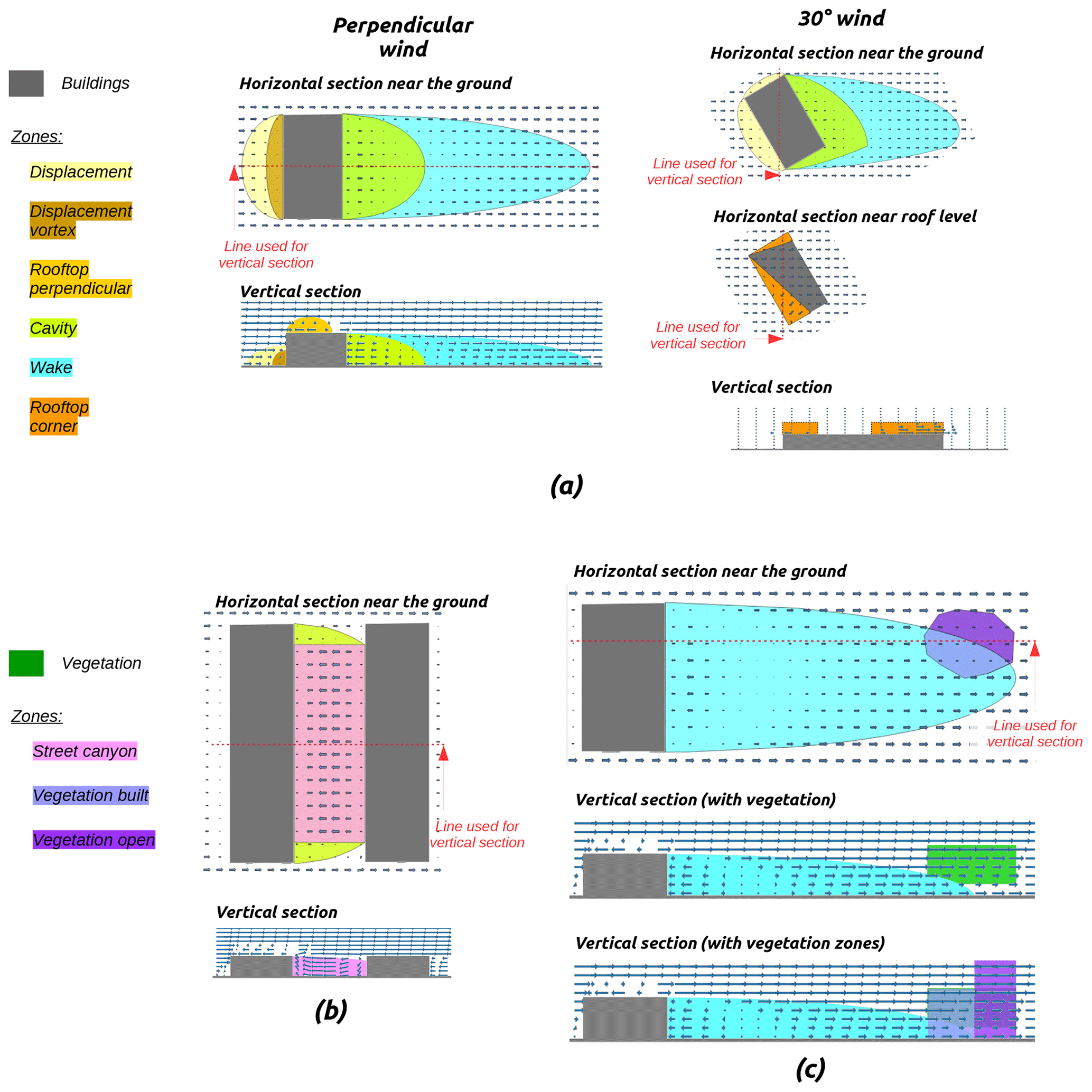
Figure 1 Illustration of the nine zones used in URock to initialize the wind field: (a) zones created by isolated buildings, (b) zones created between adjacent buildings, and (c) zones created within vegetation.

The size of each of these zones is calculated from obstacle properties (such as height, length, and width for building or attenuation capacity for the vegetation). The wind speed and wind direction depend on the zone type and location within the zone (distance to the wall, the ground, or the end of the zone). More information about each of the zones will be given in Sect. 2.3.2 (building zone size), 2.3.3 (vegetation zone size), and 2.3.4 (building and vegetation wind factors).

The wind field is then numerically balanced in order to make it physically relevant with the constraint to minimize the differences with the initial wind field.

The algorithm used in URock is based on the following procedure (illustrated in Fig. 2).

1. Create URock geometries: the input geographical data are initialized into the format needed for the URock calculations.

2. Derive the effect of all obstacles on the wind: some morphometric properties of the study area are calculated and can be used to set a mean wind profile.

3. Derive the effect of individual obstacles on the wind: each obstacle is considered individually to set the initial wind factor near buildings and within vegetation.

4. Calculate wind speed: the 3D wind speed components are initialized for each cell of the domain and then used in the numerical solver to obtain the final balanced wind field.

Figure 2 Overall methodology used by the URock model.

Figure 3 Procedure used to create the URock geometries.

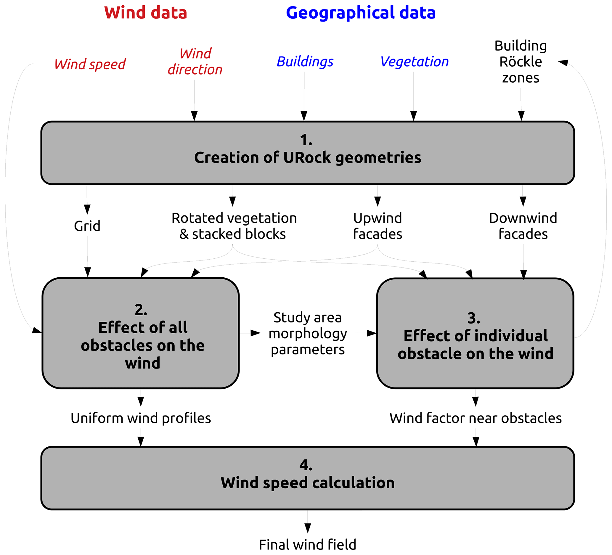
Each step of this procedure will be described in the following subsections.

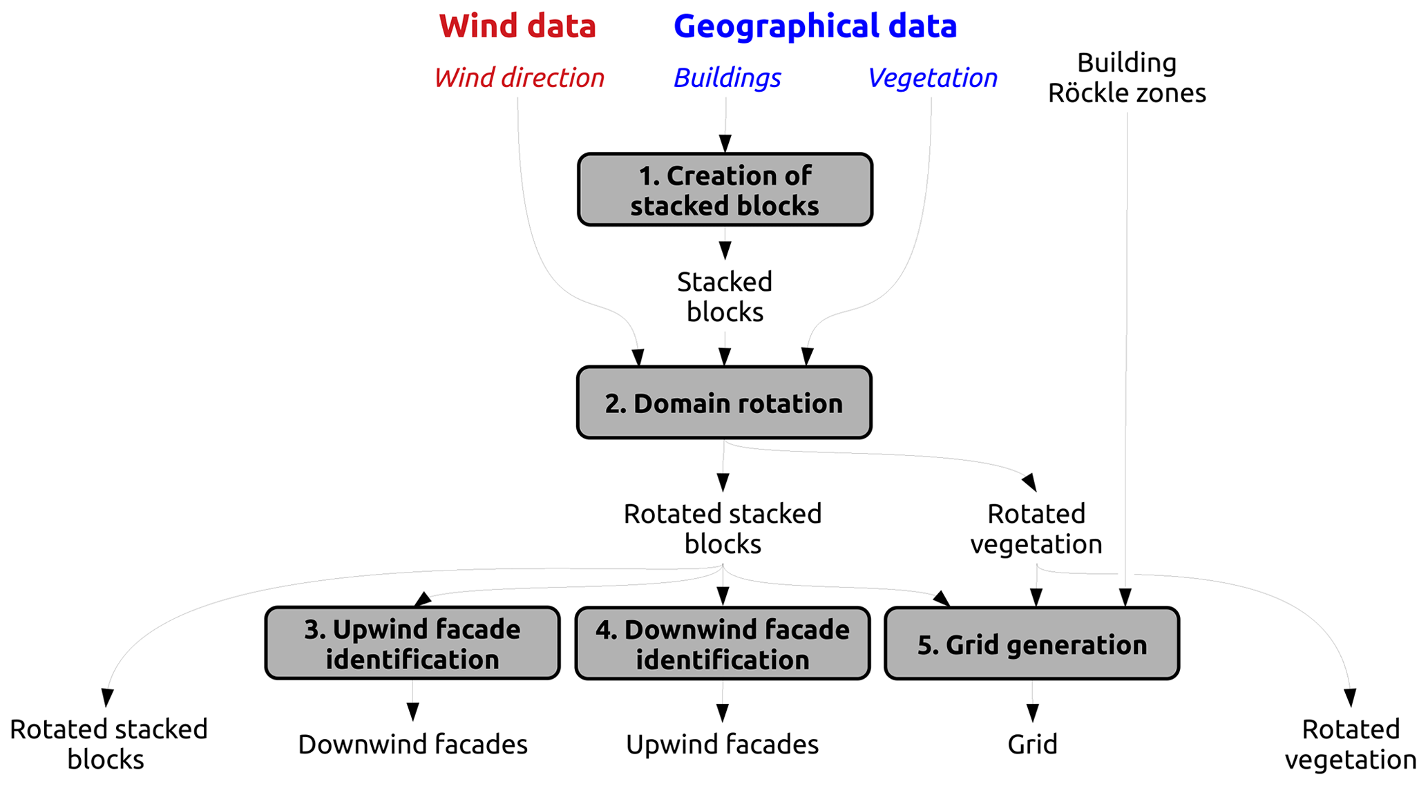
2.1 Creation of URock geometries

This step is dedicated to (i) the transformation of standard input vector geometries into a format that facilitates the wind speed initialization and (ii) the creation of the grid used for numerical solving. The following processes are used (Fig. 3). First, individual buildings are converted to stacked blocks. Then, the entire domain (buildings and vegetation) is rotated to have the wind coming from the north. Last, a 3D grid of rectangular-based cells is created, and the facades located upwind as well as those located downwind are identified.

2.1.1 Creation of stacked blocks

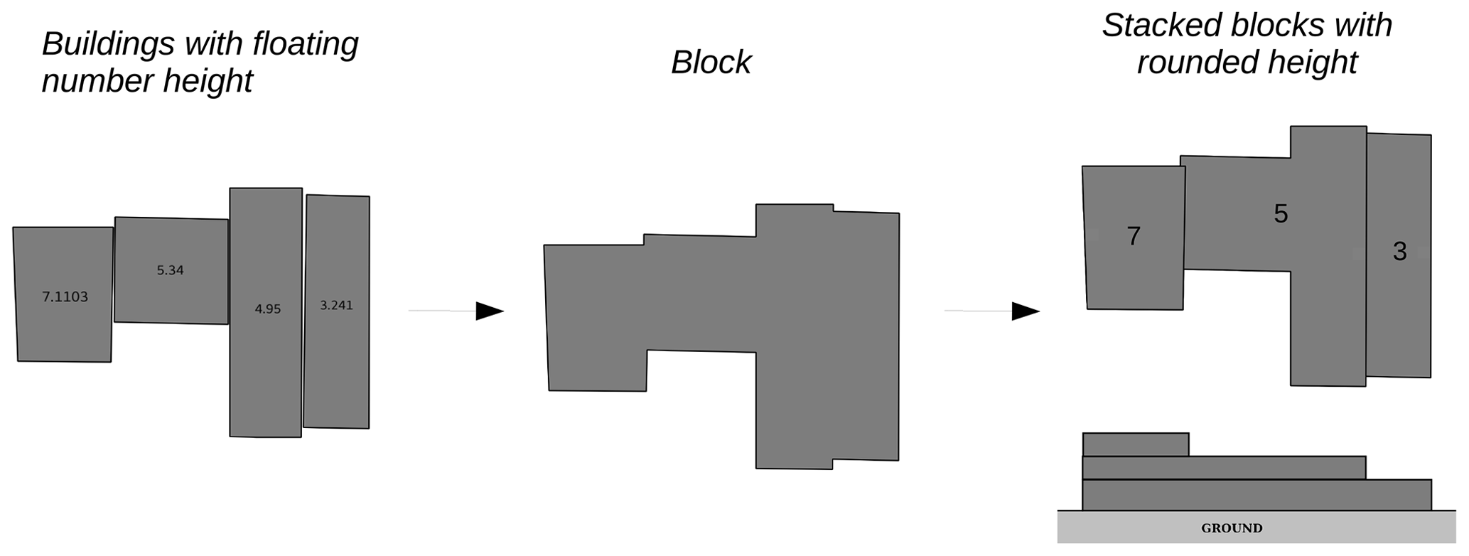
Buildings may have an oversampled number of points, which may result in a considerable number of Röckle zones (some of the zones are created for each unique segment) and thus results in low computation efficiency. In order to avoid such an issue, building geometries are first simplified by removing unnecessary points¹.

The size of a Röckle zone depends on the size of the obstacle. In URock, buildings touching each other but having a different height are transformed into vertically stacked blocks as shown in Fig. 4 – the method also used in QUIC-URB. A preliminary task is to merge buildings touching each other or within a given distance to each other. A buffer is created around each building² and the footprints touching each other are spatially joined. Then, we round building height values to the nearest integer and create as many stacked blocks as there are isolated blocks of the same height.

Figure 4 Method used to convert buildings to stacked blocks.

2.1.2 Domain rotation

All obstacles are rotated in order to have the wind coming downward to simplify the equations used in the initialization step. The rotation center is defined as the top right corner of the smallest bounding box containing all obstacles.

2.1.3 Upwind facade identification

Each facade (defined as an individual segment belonging to a given stacked block) facing the wind is identified in order to apply the displacement zone scheme. This scheme affects the area from the bottom of the facade up to 60 % of the facade height. Thus, first several facades belonging to (or nearby) the same vertical plan are merged in order to avoid an unexpected displacement zone scheme as illustrated in Fig. 5a³. The facade base height $H_{{\mathrm{FB}}_{i+\mathrm{1}}}$ ($H_{{\mathrm{FB}}_{\mathrm{1}}}$ in Fig. 5b) of the upper stacked block is then set to the base height of the bottom stacked block.

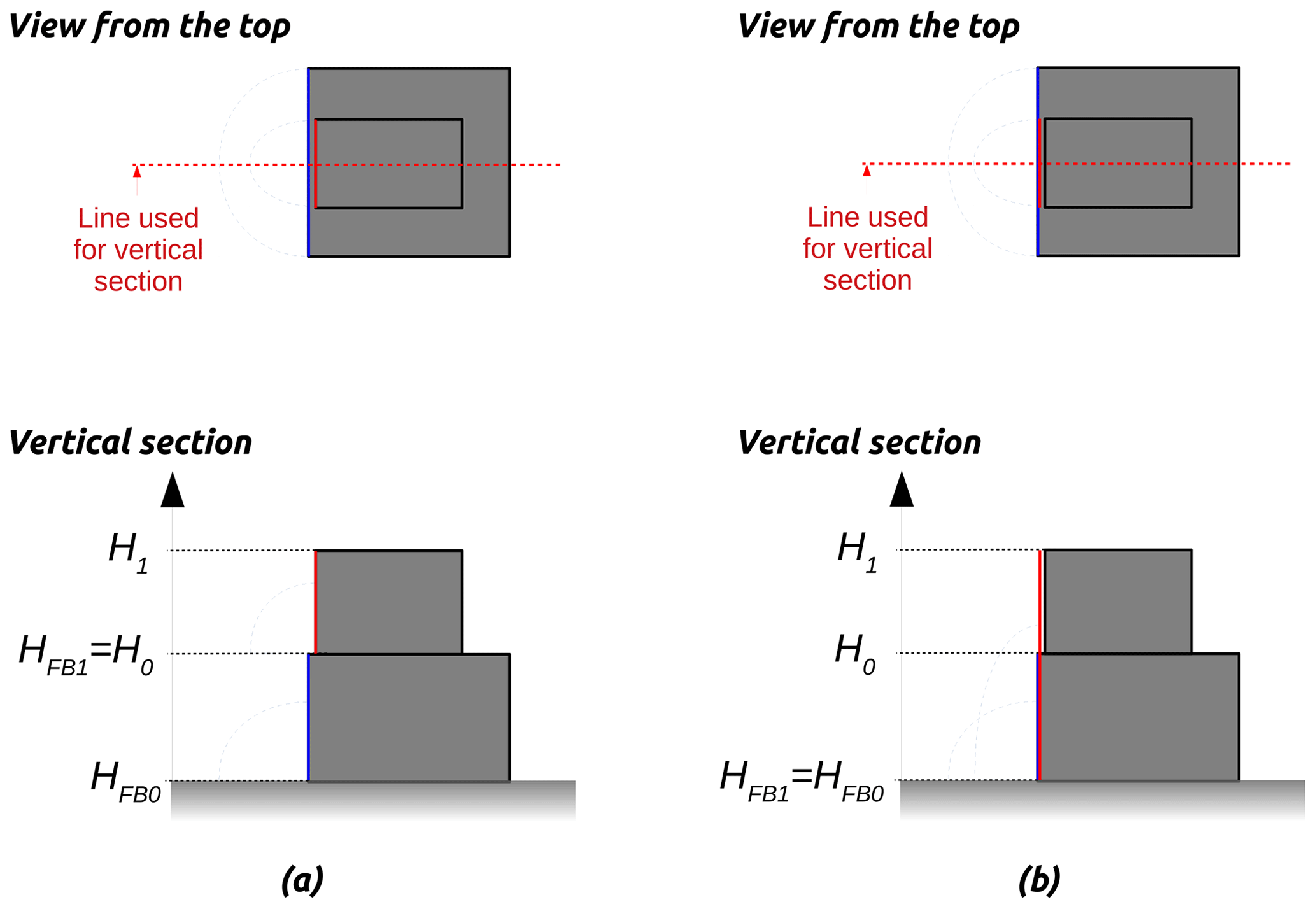
Figure 5 Facade base height and displacement zone of an upper stacked block if the facade is (a) outside or (b) within the snapping tolerance.

2.1.4 Downwind facade identification

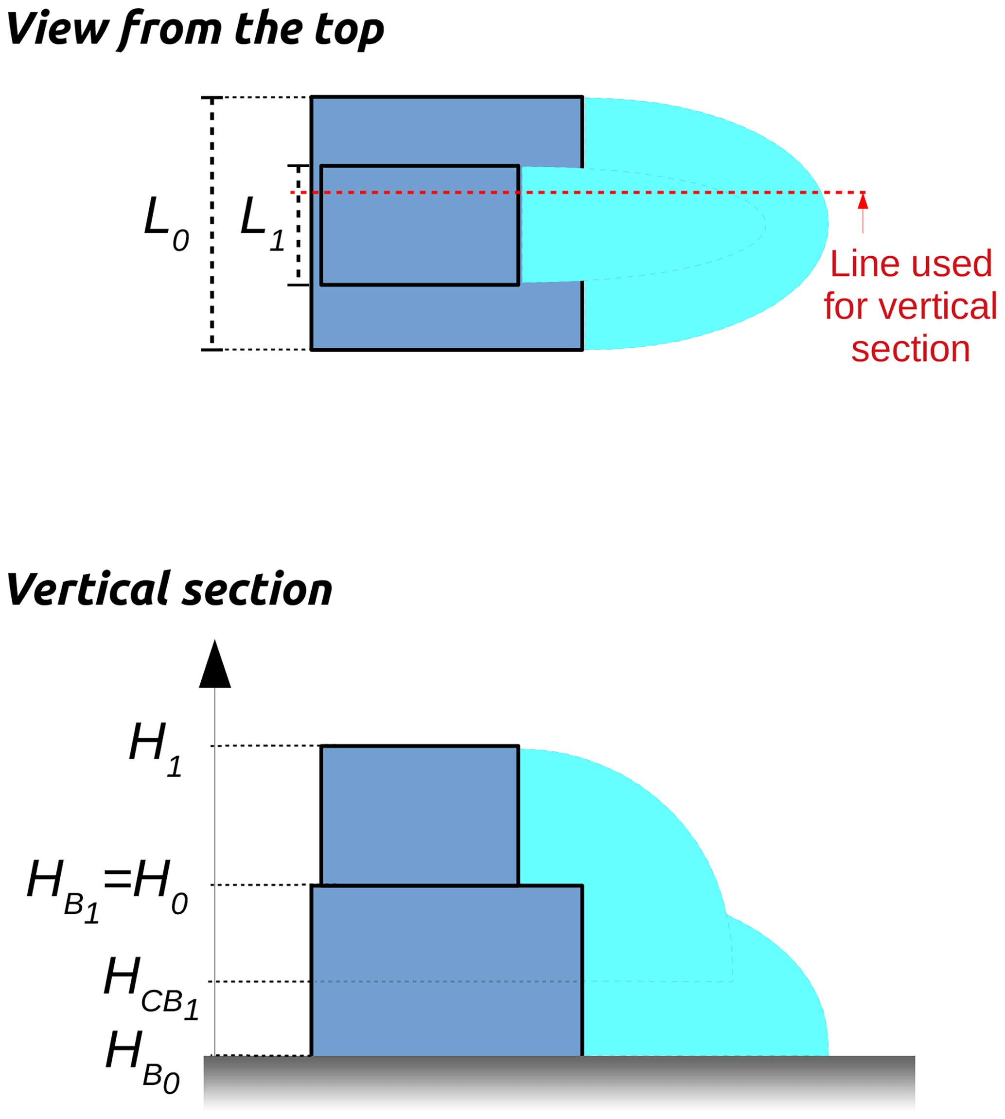
Each downwind facade (defined as a linestring – multisegments connected to each other) is identified in order to apply the cavity and wake zone schemes. Wake zones are defined from the ground, while cavity zones start at the cavity base height (H_CB). In URock, the cavity zone of a stacked block i may alter the cavity zone of the stacked block i−1 located below up to its cavity base height ($H_{{\mathrm{CB}}_i}$ – Fig. 6). This property is defined Eq. (1) (Brown et al., 2009a):

$$\begin{array}{}\text{(1)}& H_{{\mathrm{CB}}_i}=H_{{\mathrm{B}}_i}-{\displaystyle \frac{L_i}{L_{i-\mathrm{1}}}}\cdot (H_{i-\mathrm{1}}-H_{{\mathrm{B}}_{i-\mathrm{1}}}),\end{array}$$

where $H_{{\mathrm{B}}_i}$ is the base height of stacked block i above ground level, $H_{{\mathrm{B}}_{i-\mathrm{1}}}$ is the base height of stacked block i−1 above ground level, H_i−1 is the top height of stacked block i−1 above ground level, L_i is the cross-wind width of stacked block i, and L_i−1 is the cross-wind width of stacked block i−1.

Figure 6 Cavity base zone extension for downwind facades of an upper stacked block.

2.1.5 Grid generation

The grid of rectangular-based cells is created according to a horizontal and a vertical resolution set by the user. The size of the grid is defined as an extend distance beyond the built Röckle zones and vegetation boundaries (Fig. 7). By default, the values for the extensions are 60, 40, and 20 m, respectively, for the along-wind, cross-wind, and vertical axis⁴.

Figure 7 Domain size definition according to along-wind zone, cross-wind zone, and vertical extents.

2.2 Effect of all obstacles on the wind

The vertical wind profile is initialized considering mean roughness properties of the study area (Fig. 8).

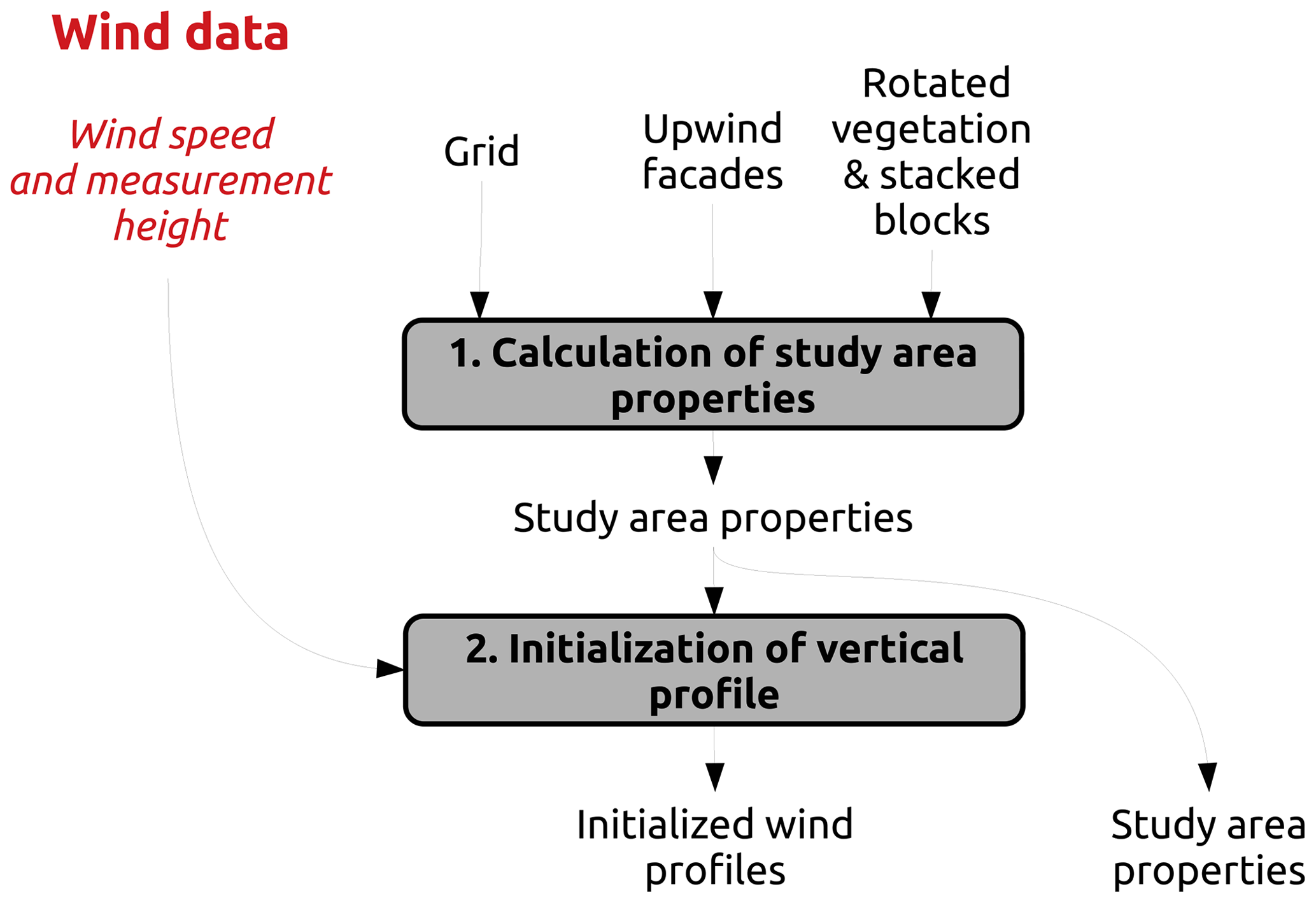
Figure 8 The procedure used takes into account the effect of all obstacles on the wind field.

2.2.1 Calculation of study area properties

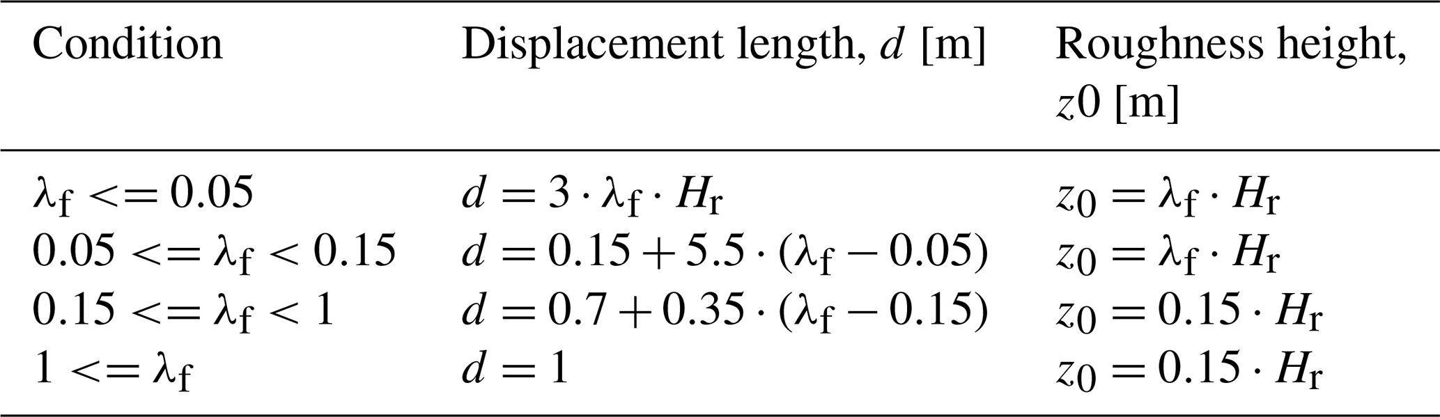
The roughness height (z₀) and displacement length (d) are both calculated as a unique value characterizing the entire study area. The method described by Hanna and Britter (2002) is used. First, the normalized frontal area (λ_f) is calculated as the ratio between the projected frontal area of an obstacle facing the wind (A_f) and the horizontal area of the smallest rectangle containing all buildings and vegetation (A_T). Then z₀ and d are calculating based on the area-weighted geometric mean obstacle height (H_r) and the λ_f value. Note that the equations vary as a function of λ_f (Table 1).

Table 1 Displacement length and roughness height equations depending on the normalized frontal area value. Note that Hanna and Britter (2002) specified that these relations are valid for an upper H_r limit of about 20 m; thus, it may lead to higher error if applied to neighborhoods consisting of skyscrapers.

2.2.2 Initialization of vertical profile

In this URock version, the vertical wind speed profile is set homogeneously on the entire calculation domain. Three possible choices are currently available to set the vertical profile using the following.

1. The first is a power law, as defined by Pardyjak and Brown (2003) (Eq. 2),

   $$\begin{array}{}\text{(2)}& V\left(z\right)=V_{\mathrm{ref}}\cdot {\left({\displaystyle \frac{z}{z_{\mathrm{ref}}}}\right)}^p,\end{array}$$

   where V(z) is the wind speed at height z above ground level, V_ref is the reference wind speed observed (or modeled) at the reference height, z_ref is the height above ground level of the reference wind speed, and $p=\mathrm{0.12}\cdot z_{\mathrm{0}}+\mathrm{0.18}$ is the exponent of the power law where z₀ is the roughness height of the study area (Matzarakis and Endler, 2009).

2. The second is an urban profile, defined as an exponential increase within the canopy (Cionco, 1972) and logarithmic increase above the canopy (Eq. 3),

   $$\begin{array}{}\text{(3)}& {\displaystyle }V\left(z\right)=\left\{\begin{array}{ll}{V}_{\mathrm{ref}}\cdot \exp (a\cdot (\frac{z}{H_{\mathrm{r}}}-\mathrm{1}\left)\right)& \text{if}z<H_{\mathrm{r}}\\ V_{\mathrm{ref}}\cdot \frac{\log \left(\frac{z-d}{z_{\mathrm{0}}}\right)}{\log z_{\mathrm{ref}}{z}_{\mathrm{0}}}& \text{otherwise},\end{array}\right.\end{array}$$

   where $a=\mathrm{9.6}\cdot {\mathit{\lambda }}_{\mathrm{f}}$ is the attenuation coefficient (Macdonald, 2000), λ_f is the normalized frontal area, H_r is the area-weighted geometric mean height of all obstacles, z₀ is the roughness height, and d is the displacement length (Table 1)

3. The third is a user-defined profile.

The first two solutions need a reference height, the corresponding wind speed, and information about the roughness of the area as input, while the third solution needs to have wind speed observed and/or modeled at several heights in the atmosphere.

2.3 Effect of individual obstacles on the wind

Obstacles locally alter the wind field: wind direction and/or wind speed may be modified within vegetation and around buildings. The Röckle approach is applied to set an initial wind factor to those locations using seven building schemes and two vegetation ones (Fig. 9). First, stacked block properties are calculated. Then, building and vegetation Röckle zone boundaries are identified and the wind factor corresponding to each zone is calculated. Last, some rules are set to keep only one wind factor value when two (or more) Röckle zones are overlaid.

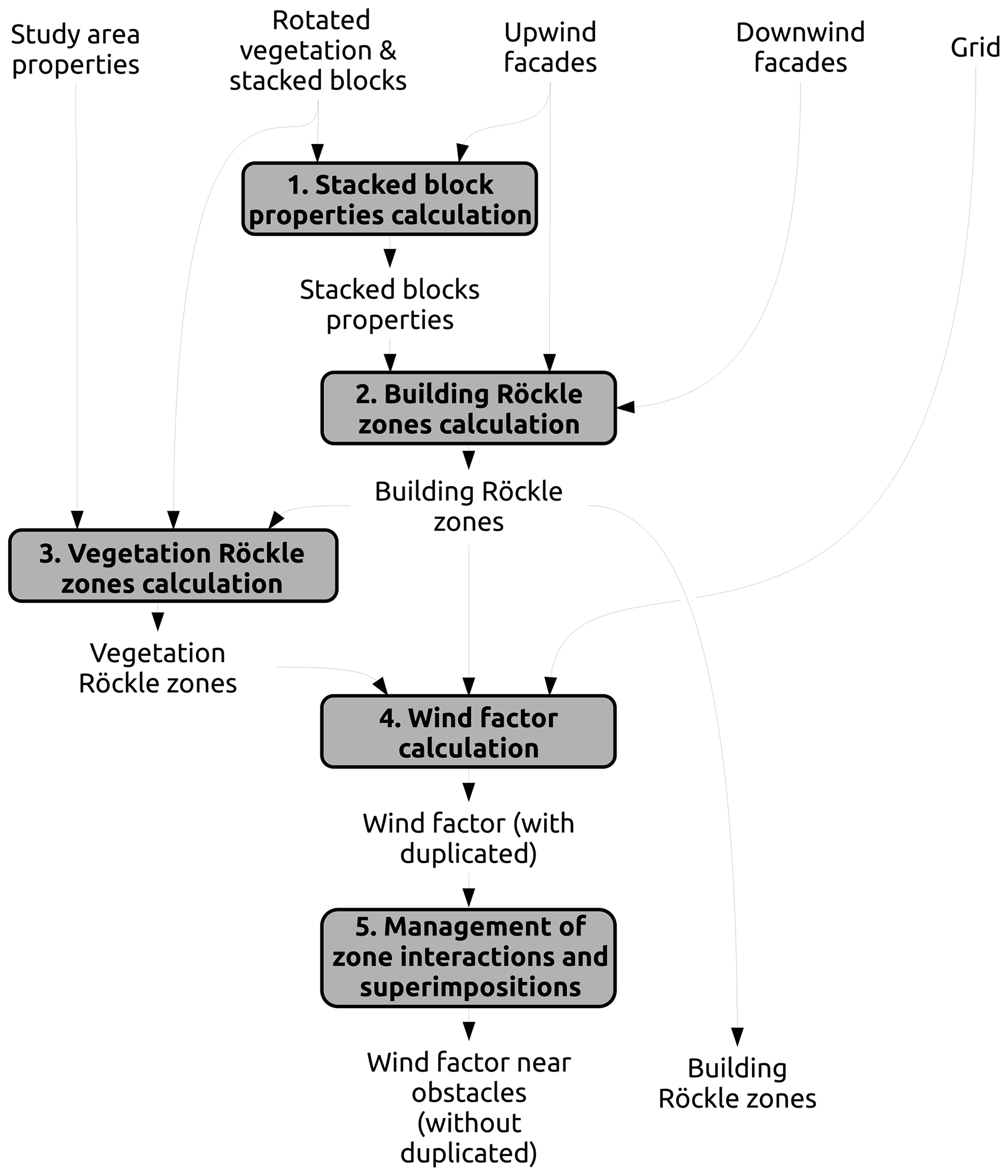
Figure 9 Procedure used to take into account the effect of each individual obstacle on the wind field.

2.3.1 Calculation of stacked block properties

The stacked block height, effective width (cross-wind width, W_eff), and effective length (along-wind length, L_eff) are the three input parameters used to calculate the building zones. While the definition of the first one has not changed over QUIC-URB versions (difference in height between the top and the base of a stacked block), the definitions of the two others have been updated by Nelson et al. (2008) to improve the accuracy of the estimated wind field when the wind is not perpendicular to the facade of a rectangular building (Fig. 10).

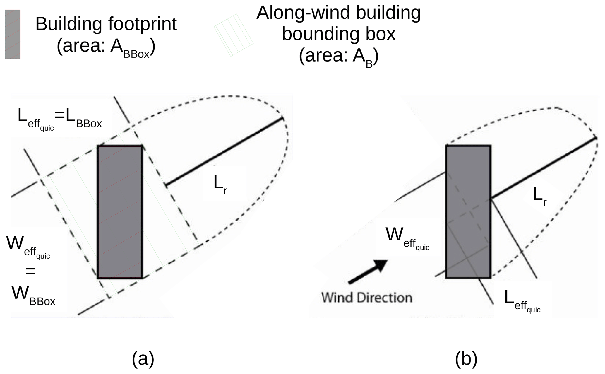
Figure 10 QUIC-URB method to calculate the building effective width and building effective length (a) before and (b) after modifications proposed by Nelson et al. (2008). Source: adapted from Nelson et al. (2008).

However, their modified algorithm only works for a rectangular shape, whereas our stacked blocks may have any shape. Thus, the effective width and length are calculated using Eqs. (4) and (5), respectively.

$$\begin{array}{}\text{(4)}& {\displaystyle }{W}_{\mathrm{eff}}=W_{\mathrm{BBox}}\cdot {\displaystyle \frac{A_{\mathrm{B}}}{A_{\mathrm{BBox}}}}\text{(5)}& {\displaystyle }{L}_{\mathrm{eff}}=L_{\mathrm{BBox}}\cdot {\displaystyle \frac{A_{\mathrm{B}}}{A_{\mathrm{BBox}}}}\end{array}$$

Here, W_eff is the effective width of the stacked block in URock, L_eff is the effective length of the stacked block in URock, W_BBox is the cross-wind width of the stacked block bounding box (corresponding to $W_{{\mathrm{eff}}_{\mathrm{quic}}}$ in Fig. 10a), L_BBox is the cross-wind length of the stacked block bounding box (corresponding to $L_{{\mathrm{eff}}_{\mathrm{quic}}}$ in Fig. 10a), A_B is the stacked block footprint area (see Fig. 10a), and A_BBox is the area of the stacked block bounding box (see Fig. 10a).

2.3.2 Building Röckle zone calculation

This section contains a partial description of the building Röckle zones calculated in URock. More details can be found in Appendix A.

Displacement zone

The displacement zone is defined as a quarter of an ellipse located on each upwind facade (see Fig. 1a) as defined by Kaplan and Dinar (1996).

Displacement vortex zone

The displacement vortex zone is defined as a quarter of an ellipse located on each upwind facade whenever the angle between the wind direction and an upwind facade-normal ${\mathit{\theta }}_{\mathrm{wind}/{\mathrm{upwind}}_{\mathrm{F}}}$ is within [-PERPENDICULAR_THRESHOLD_ANGLE, PERPENDICULAR_THRESHOLD_ANGLE] (see Fig. 1a). The default value for PERPENDICULAR_THRESHOLD_ANGLE is set to 15^∘ compared to 20^∘ in QUIC-URB (Bagal et al., 2004). The reason for this difference is that the rooftop perpendicular scheme is also activated when the upwind facade is close to perpendicular to the wind direction. The condition for activation of the rooftop perpendicular and displacement vortex differs in QUIC-URB (15^∘ for the rooftop perpendicular vortex, 20^∘ for the displacement vortex), but we chose to have consistency between these two schemes in URock. Nevertheless, the size of the zone is identical in URock and QUIC-URB (Bagal et al., 2004).

Cavity zone

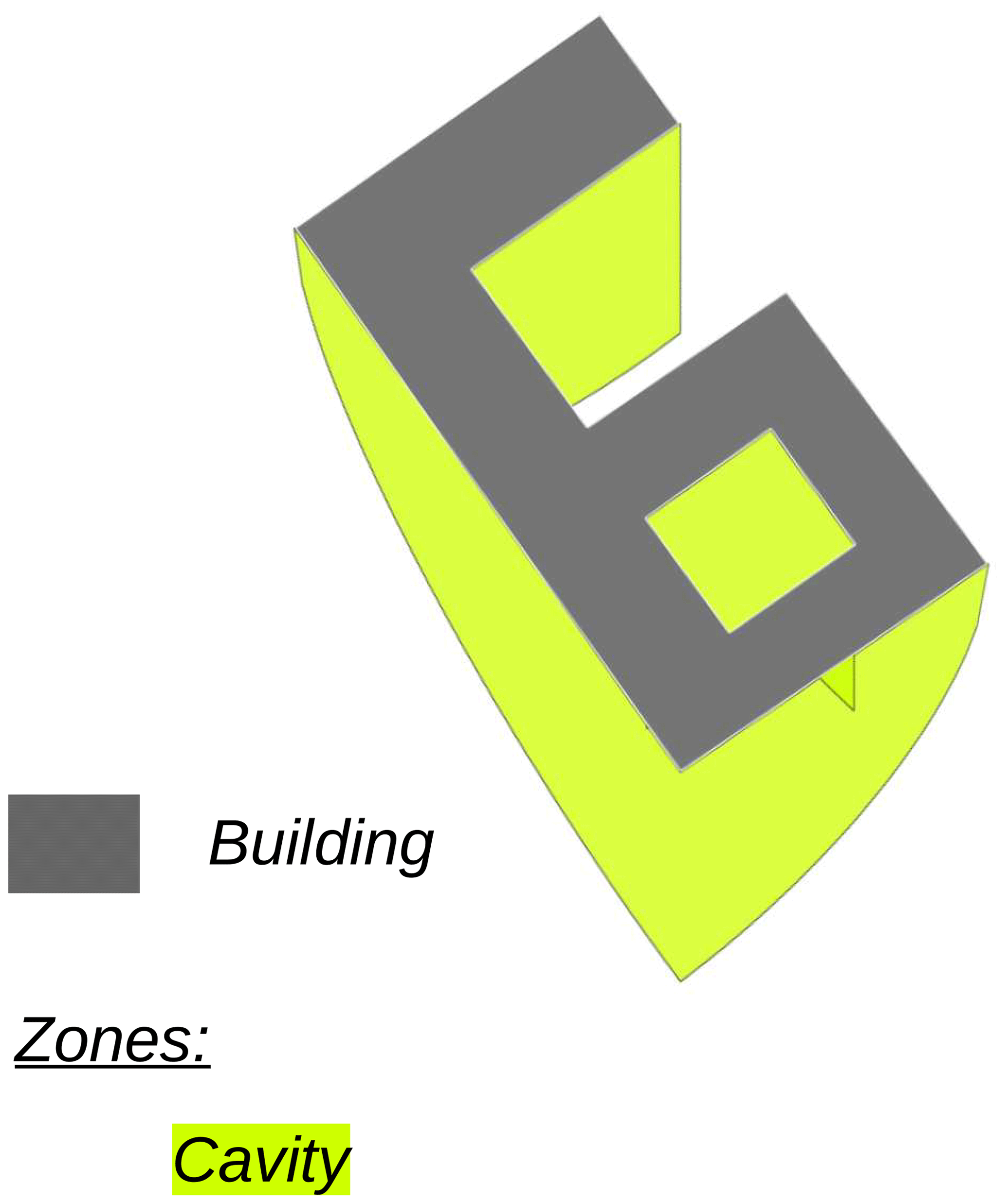
The cavity zone can be seen as a quarter of an ellipse but having a slightly modified equation. If a standard ellipse has a fixed center, the one used in URock has a center that moves along the wind direction, following the facade coordinates (see Fig. 1a). For complex stacked blocks, such as those with multiple downwind facades, this definition results in cavity zones illustrated in Fig. 11. For any downwind facade, the ellipse has the same size at a given coordinate along the cross-wind axis. This is most probably not the case in reality and should thus be further investigated in future URock versions.

Figure 11 View from the top of the cavity zones created for a complex stacked block.

Wake zone

The wake zone develops after the cavity zone. Thus, it has a similar shape but is 3 times longer along the wind axis (Kaplan and Dinar, 1996).

Rooftop perpendicular zone

The rooftop perpendicular zone is defined as half of an elliptical cylinder – sliced longitudinally along the cylinder axis and major axis of the ellipse. It is located on each rooftop with lengths consistent with the ones defined by Pol et al. (2006). It is only created when the angle between the wind direction and an upwind facade-normal ${\mathit{\theta }}_{\mathrm{wind}/{\mathrm{upwind}}_{\mathrm{F}}}$ is within [-PERPENDICULAR_THRESHOLD_ANGLE, PERPENDICULAR_THRESHOLD_ANGLE] (see Fig. 1a). The default value for PERPENDICULAR_THRESHOLD_ANGLE is set to 15^∘, the same value as in QUIC-URB (Pol et al., 2006). Note that the rooftop perpendicular zones are only defined above buildings. Since they extend from the upper edges of the upwind facades along-wind, they form oblique cylinders whenever the wind is not perpendicular to the upwind facade.

Rooftop corner zone

The rooftop corner zone is defined as a square-base oblique pyramid located on a rooftop along an upwind facade with the apex starting from the most upwind point (see Fig. 1a). The size of the zone is calculated using the equations of Bagal et al. (2004). The scheme is activated only when the angle between the wind direction and an upwind facade-normal ${\mathit{\theta }}_{\mathrm{wind}/{\mathrm{upwind}}_{\mathrm{F}}}$ is within +-[CORNER_THRESHOLD_ANGLE_MIN, CORNER_THRESHOLD_ANGLE_MAX] and the default values for CORNER_THRESHOLD_ANGLE_MIN and CORNER_THRESHOLD_ANGLE_MAX are 30 and 70^∘, respectively.

Street canyon zone

The street canyon zone is created between two stacked blocks when the upstream building cavity zone intersects the upwind facade of a downstream building.

2.3.3 Vegetation Röckle zone calculation

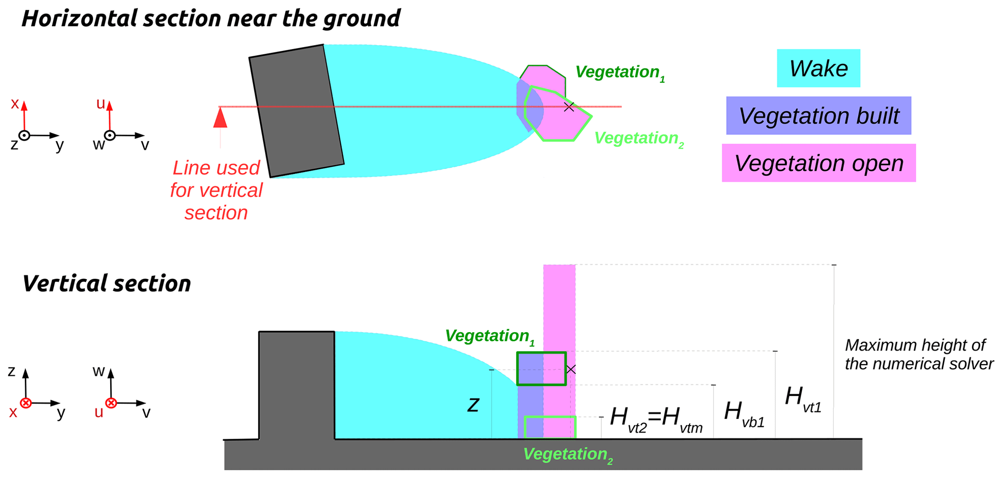
Similarly as QUIC-URB (Nelson et al., 2009), two different schemes are dedicated to the vegetation in URock: one when the vegetation is located within a building influence (vegetation in a built-up area) and the other when it is far from a building influence (vegetation in an open area).

Vegetation in built-up areas

The vegetation built zone is defined wherever the wake zone of any building intersects the footprint of a vegetation patch. Only the column of air located within the vegetation canopy belongs to the zone (see Fig. 1c).

Vegetation in open areas

The vegetation open zone is defined wherever the footprint of a vegetation patch is not intersected by any building wake zone. The entire column of air (below, within, and above the vegetation) belongs to the zone (see Fig. 1c).

2.3.4 Wind factor calculation

Once the wind zones are defined, wind factors along the three vector components are set. They are defined as the fraction of the wind speed at a given height and position and are Röckle-zone-dependent. The equations used to calculate these wind factors are described in Appendix B. For a more visual representation of these equations, please refer to the wind field illustrated in Fig. 1.

2.3.5 Management of zone interactions and superimpositions

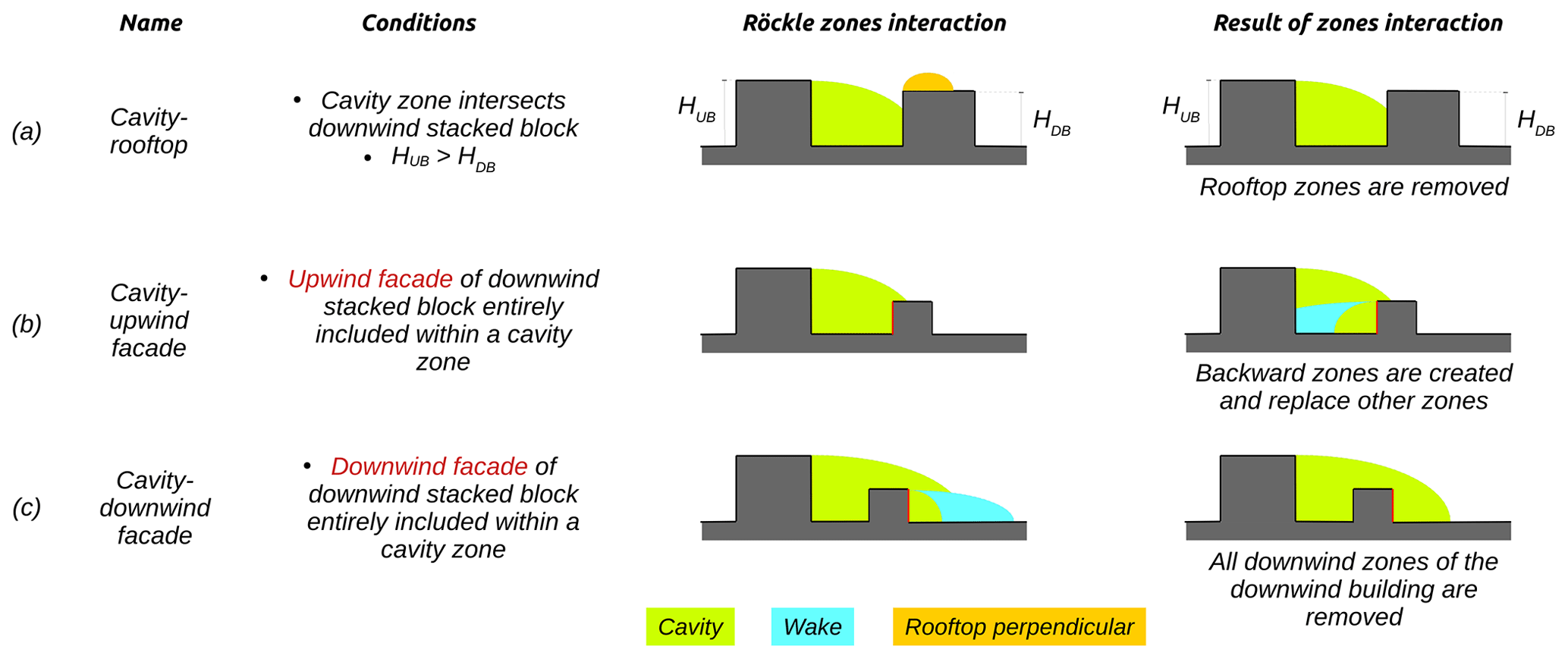
The workflow of URock for dealing with zone interactions and superimpositions is mainly based on the QUIC-URB method. For additional details on the adopted method, which also motivated our decisions regarding the URock method, the reader is referred to Brown et al. (2009a, 2013). Although the philosophy and main physical reason for their method are well described, it is difficult to discern a clear algorithm in the QUIC-URB method. This section attempts to fill this gap.

Concerning zone interactions, the cavity zone of any stacked block may remove or create zones under certain conditions. URock removes any rooftop zone and any downwind building zone, respectively, for cavity–rooftop and cavity–downwind facade interactions (Fig. 12a and b). Backward cavity and wake zones are also created in the case of cavity–upwind facade interaction (Fig. 12c). They have the same size as forward cavity and wake zones, except that they start from upwind facades instead of downwind facades and thus go in the opposite direction. Their wind factor for the same distance from the wall and height is also identical in forward cavity and wake zones, except that they are multiplied by a coefficient of attenuation. The value of this coefficient depends on the location of the upwind facade within the cavity zone. The value of the cavity zone wind factor at the top of the upwind facade is taken as the attenuation coefficient. Backward zone creation removes all downwind zones (cavity, wake, and street canyon), which may be at this position. The definition of the upwind stacked block starts from the upper part of the backward zones instead of the ground.

Figure 12 Description and results of the Röckle zone interactions implemented in URock.

Figure 13 Workflow used to deal with zone superimposition.

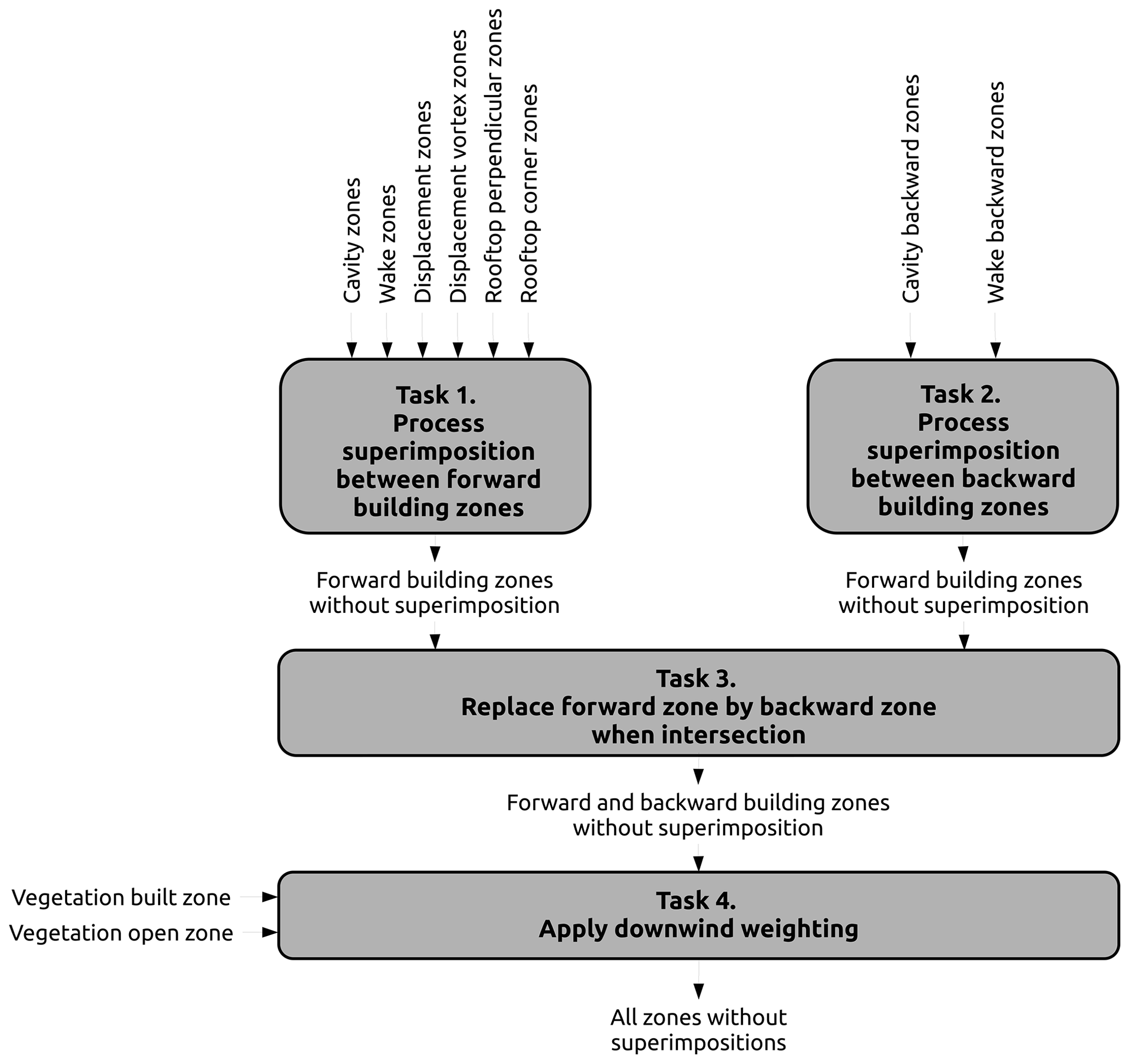
Once these interactions are solved, certain points in the domain may belong to several zones (Röckle zone superimposition). In this case, the following procedure is used to decide what rule or combination of rules applies to each of these points (presented in Fig. 13 and further described afterward).

• Task 1: only forward building zone superimpositions are solved in order to have a single wind factor per point of the space.

• Task 2: similar work is performed with backward building zones but previously weighted by forward wake zones.

• Task 3: forward and backward wind factors are merged (backward wind factors are used in the case of zone intersections).

• Task 4: the resulting wind factors are multiplied by vegetation weights when they intersect vegetation zones.

When several zones are superimposed, most of the choices are based on the most upstream and tallest stacked block rule. It means that the zone created by the most upstream stacked block is conserved. The origin of a zone is defined by the upwind facade for rooftop and displacement zones and by the downwind one for cavity, wake, and street canyon zones. If the origin of two zones is the same (i.e., one block piled on an other), then the zone created by the upper stacked block is conserved. If the zones have been created by the same stacked block, the conserved zone is defined using the following priority order: street canyon, cavity, rooftop perpendicular, rooftop corner, displacement vortex, displacement, wake zone.

Task 1 consists of three subtasks. The first subtask resolves the superimposition between all building zones based on the previous rule. The second subtask is to deal with superimposition happening only between wake zones. The most upstream and highest stacked block rule described above is again used. The last subtask is to multiply the wind factors coming from subtask 1 by those obtained from subtask 2 only if those from subtask 2 come from a more upstream and the highest stacked block.

Task 2 is quite similar to task 1. The first subtask is to resolve backward cavity and backward wake zones, but conserving zones created by the most downstream stacked block instead of the most upstream one. The second subtask is applied using only the backward wake zone using the most downstream stacked block rule. The third subtask is also a combination of the results from subtask 1 and subtask 2 but using the most downstream stacked block rule. The fourth additional task is to multiply the wind factors from the previous task 3 by the ones obtained in task 1, subtask 2.

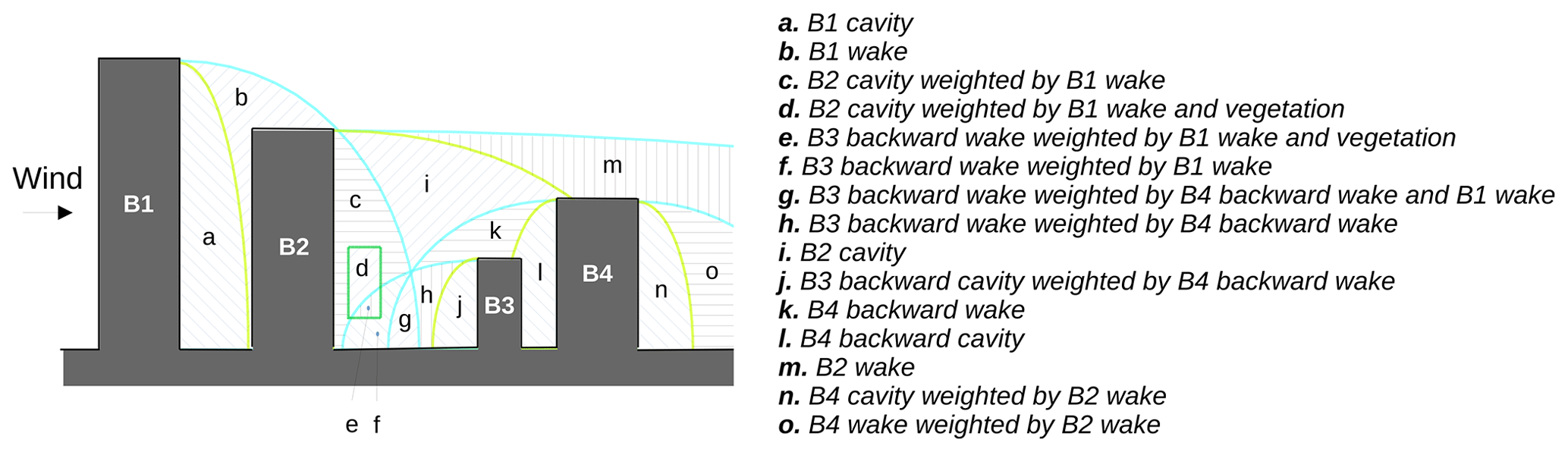
Tasks 3 and 4 are simpler; thus, the description given previously is sufficient to understand what is performed. Figure 14 illustrates the result of the whole superimposition procedure (considering only five zone types for the sake of simplicity: vegetation, cavity, wake, backward cavity, and backward wake).

Figure 14 Example of zones resulting from the superimposition workflow.

2.4 Wind speed calculation

The wind speed field calculation is performed in two steps: first, the wind speed is initialized for all points of the domain, and second, the numeric wind solver is applied to balance the wind flow (Fig. 15).

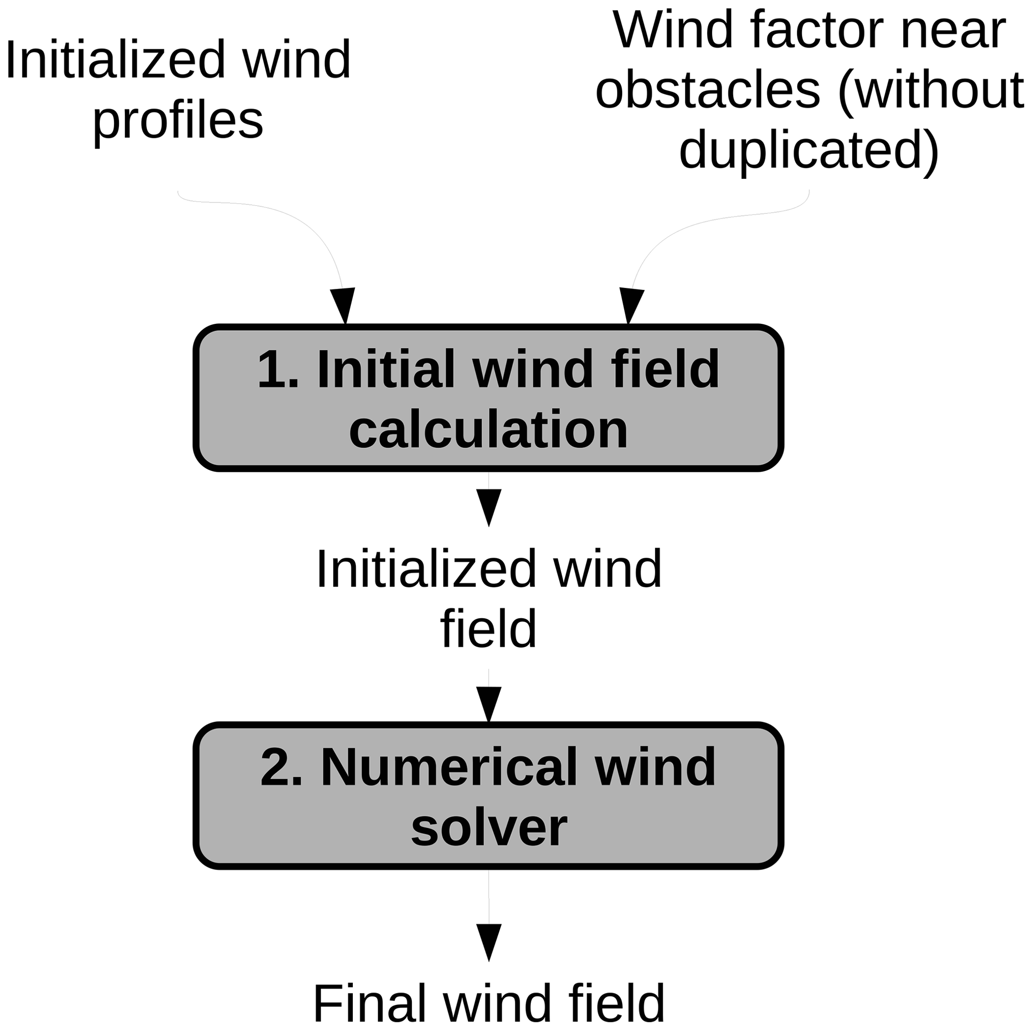
Figure 15 Procedure used to calculate wind speed field from vertical wind profile and wind factors.

2.4.1 Initial wind field calculation

Once the wind factors (WFs) are calculated and unique for any point of the space, they are used along with the vertical wind profile to initialize the wind speed field using Eq. (6).

$$\begin{array}{}\text{(6)}& {\displaystyle }\left\{\begin{array}{l}{U}_{\mathrm{0}}(x,y,z)={\mathrm{WF}}_U(x,y,z)\cdot V_{\mathrm{wp}}(x_{\mathrm{ref}},y_{\mathrm{ref}},z_{\mathrm{ref}})\\ V_{\mathrm{0}}(x,y,z)={\mathrm{WF}}_V(x,y,z)\cdot V_{\mathrm{wp}}(x_{\mathrm{ref}},y_{\mathrm{ref}},z_{\mathrm{ref}})\\ W_{\mathrm{0}}(x,y,z)={\mathrm{WF}}_W(x,y,z)\cdot V_{\mathrm{wp}}(x_{\mathrm{ref}},y_{\mathrm{ref}},z_{\mathrm{ref}})\end{array}\right.\end{array}$$

Here $U_{\mathrm{0}}(x,y,z)$, $V_{\mathrm{0}}(x,y,z)$, and $W_{\mathrm{0}}(x,y,z)$ represent the wind speed along the x, y, and z axis, respectively, for the point with coordinates x, y, and z; WF${}_U(x,y,z)$, WF${}_V(x,y,z)$, and WF${}_W(x,y,z)$ represent the wind factor along the x, y, and z axis, respectively, for the point with coordinates x, y, and z (default 1 is not covered by any Röckle zone); and V_wp(x_ref,y_ref, and z_ref) represents the along-wind (y-axis) wind speed for the point at the reference position of the zone.

Three definitions of V_wp(x_ref,y_ref, and z_ref) exist depending on the zone.

1. The wind speed is taken at the top of the facade that corresponds to the beginning of the zone (note that in the current version of URock, the entire domain has the same vertical wind profile, and thus only z_ref will affect the $V_{\mathrm{wp}}(x_{\mathrm{ref}},y_{\mathrm{ref}},z_{\mathrm{ref}})$ value):

   1. upwind facade for displacement, displacement vortex, backward cavity, and backward wake zones;

   2. downwind facade for cavity and street canyon.

2. The wind speed is taken at the location of the point of interest (x, y, z): wake, vegetation built, and vegetation open zones (all weighting zones).

3. The wind speed is taken at the reference height as used in Eqs. (B5) and (B6) (rooftop perpendicular and rooftop corner zones).

2.4.2 Numerical wind solver

The last step of the methodology consists of balancing the airflow while minimizing the modifications of the initialized wind field. To achieve this, the Lagrange multiplier (λ) in Eq. (7) is calculated. First, the initial wind field calculated at the center of each voxel is linearly interpolated to the voxel faces. Afterwards, an iterative process is used to calculate the 3D values of λ (for more detail concerning the numerical solver, please see Pardyjak and Brown, 2003).

$$\begin{array}{}\text{(7)}& \begin{array}{rl}E(u,v,w,\mathit{\lambda })& =\underset{V}{\int }\left[{\mathit{\alpha }}_{\mathrm{1}}^{\mathrm{2}}\cdot (u-u_{\mathrm{0}}{)}^{\mathrm{2}}+{\mathit{\alpha }}_{\mathrm{1}}^{\mathrm{2}}\cdot (v-v_{\mathrm{0}}{)}^{\mathrm{2}}+{\mathit{\alpha }}_{\mathrm{2}}^{\mathrm{2}}\right.\\ & \left.\cdot (w-w_{\mathrm{0}}{)}^{\mathrm{2}}+\mathit{\lambda }\cdot \left({\displaystyle \frac{\partial u}{\partial x}}+{\displaystyle \frac{\partial u}{\partial x}}+{\displaystyle \frac{\partial u}{\partial x}}\right)\right]\\ & \cdot \mathrm{d}x\cdot \mathrm{d}y\cdot \mathrm{d}z\end{array}\end{array}$$

Here $E(u,v,w,\mathit{\lambda })$ is the function to minimize V, the whole domain volume; α₁ and α₂ are the Gaussian precision moduli that can be used to favor modification of the wind field toward the horizontal or vertical direction (by default set to 1); u, v, and w represent the balance wind field; u₀, v₀, and w₀ represent the initial wind field; and dx, dy, and dz represent the domain resolution along the x, y, and z axis

If ${\mathit{\lambda }}_{i,j,k}^t$ and ${\mathit{\lambda }}_{i,j,k}^{t+\mathrm{1}}$ are λ values for cells located at coordinates i, j, and k at iteration steps t and t+1, respectively, we stop the iterative process when the condition described Eq. (8) is met:

$$\begin{array}{}\text{(8)}& E=\sum _{i=\mathrm{1}}^{nx}\sum _{j=\mathrm{1}}^{ny}\sum _{k=\mathrm{1}}^{nz}\mathrm{|}{\mathit{\lambda }}_{i,j,k}^{t+\mathrm{1}}-{\mathit{\lambda }}_{i,j,k}^t\mathrm{|}<\mathit{ϵ},\end{array}$$

where ϵ the threshold value to stop iterations (default 0.0001).

Last, the wind velocity field is updated using the final λ values (Eq. 9). Note that the wind speed orthogonal to the boundary of a solid cell should be zero $\left(\frac{\partial \mathit{\lambda }}{\partial n}\right)$ and at the inflow–outflow boundary, the initial wind profile should not be modified (λ=0).

$$\begin{array}{}\text{(9)}& {\displaystyle }\left\{\begin{array}{ll}u& =u_{\mathrm{0}}+\frac{\mathrm{1}}{\mathrm{2}\cdot {\mathit{\alpha }}_{\mathrm{1}}^{\mathrm{2}}}\cdot \frac{\partial \mathit{\lambda }}{\partial x}v=v_{\mathrm{0}}+\frac{\mathrm{1}}{\mathrm{2}\cdot {\mathit{\alpha }}_{\mathrm{1}}^{\mathrm{2}}}\cdot \frac{\partial \mathit{\lambda }}{\partial y}w=w_{\mathrm{0}}\\ & +\frac{\mathrm{1}}{\mathrm{2}\cdot {\mathit{\alpha }}_{\mathrm{2}}^{\mathrm{2}}}\cdot \frac{\partial \mathit{\lambda }}{\partial z}\end{array}\right.\end{array}$$

3 Model implementation

Currently, URock 2023a is openly available as a QGIS plug-in in the Zenodo repository⁵. The tool development is currently performed on GitHub at the UMEP repository⁶. It is mainly coded in Python and can be used as a stand-alone Python library. Most of the spatial analysis is performed using the H2GIS spatial database (Bocher et al., 2015). The wind solver is based on the Numba Python library to boost the calculations.

In QGIS, the following minimal information is needed.

• Geographical information: one GIS layer for buildings or one for vegetation, with at least a single attribute for a roof or crown-top height from the ground, respectively.

• Wind conditions: wind speed and direction at a given height or a wind direction and a file containing a wind profile (.csv file with height as the first column, wind speed as the second column).

• Cell size: the vertical and horizontal resolution used for the wind solver.

• Output height: one height or several heights for which the wind field is needed.

As output, URock 2023a can save the 3D wind field in a NetCDF file or wind information along one or several planes at a height defined by the user in two formats: a raster file, containing the absolute wind speed, or a vector file, containing horizontal wind speed, vertical wind speed, absolute wind speed, and wind direction.

URock 2023a is integrated within the QGIS plug-in called UMEP. Like any UMEP processor, URock comes with its own preprocessor called urock_prepare and its own post-processor called urock_analyser (see workflow Fig. 16). The first is useful if the user has a building footprint (or vegetation) without height attribute. If the user has a digital surface model (for building or vegetation) and a digital elevation model, urock_prepare can be used to generate building and vegetation files in the right format. The post-processor is used once URock 2023a has been run (and a NetCDF file saved) to plot a sectional view of the wind along a line or a vertical wind profile averaging the wind within a polygon. These two modules are already available in UMEP, and their development is performed on GitHub⁷.

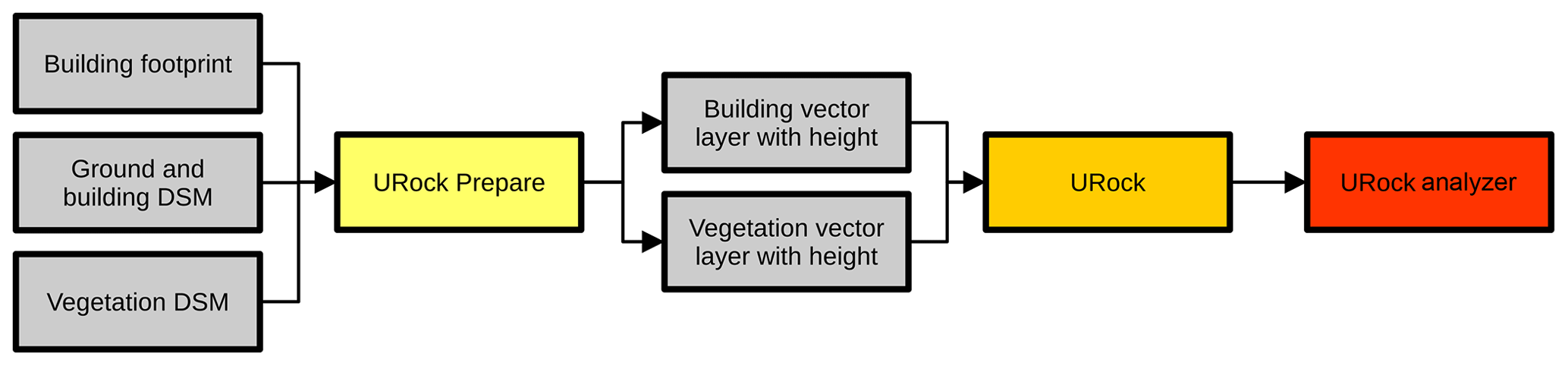
Figure 16 Workflow used to generate and analyze a wind field from raster data using URock and its related preprocessor and post-processor.

4 Model evaluation

In this section, URock (version 0.0.1) simulations are compared to QUIC-URB (version 6.4.1 in MATLAB R2020b) simulations and wind tunnel measurements for both simple and more complex cases. Vertical and horizontal resolutions are set identically in URock and QUIC-URB. Preliminary investigations have shown a very limited effect of resolution on accuracy. Thus, the main motivation for the resolution chosen in this paper is to facilitate the visual comparison between the model outputs and the measurements.

Spatial data and vertical wind profiles are set according to wind tunnel experiment parameters. All wind tunnel data are freely available on the AIJ website⁸.

The simulations of each AIJ case have been run using the input wind profile measured in the wind tunnel for a given wind direction. The sensors not necessarily being located at the center of a simulation cell, linear interpolation is used in order to compare the wind at the exact sensor location. Figures presented in the next subsections are created using URock and QUIC-URB outputs in QGIS for top view figures and using the module URock analyzer for the sectional view figures.

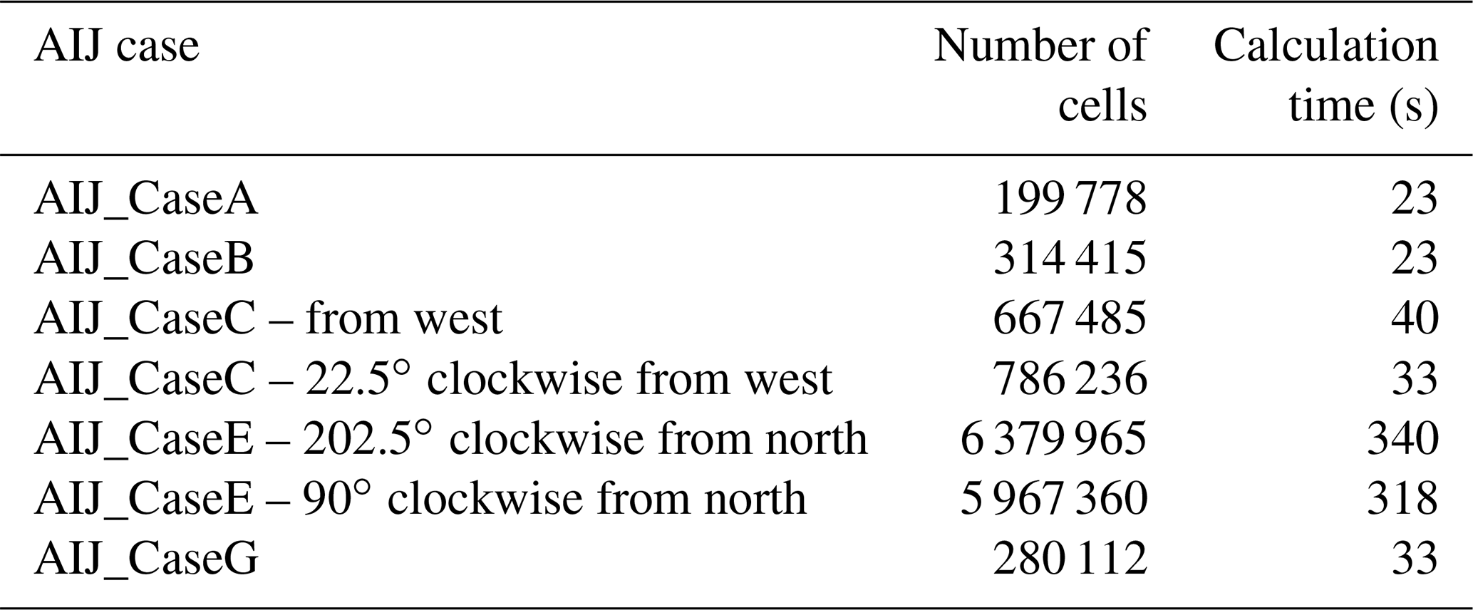
4.1 Computation time

For each of the AIJ cases simulated using the URock model, the number of cells used for the calculation and the computation time are given in Table 2. The calculations have been performed using a single processor (frequency of 2.3 GHz) on a personal computer. The installed random access memory of the computer is 16 GB. Note that the time presented also accounts for file loading (spatial information and wind conditions), initializing connection with the database used for spatial calculation, and writing output files.

Table 2 Domain size used for the URock 2023a model to simulate AIJ cases and associated computation time.

4.2 General agreement between URock and QUIC-URB

Based on the locations where the wind was observed in the AIJ wind tunnel experiment, the correlation coefficient calculated between URock and QUIC-URB is shown for horizontal, vertical, or absolute wind speed for each of the test cases (Table 3).

Table 3 Correlation coefficients between URock and QUIC-URB for each AIJ case.

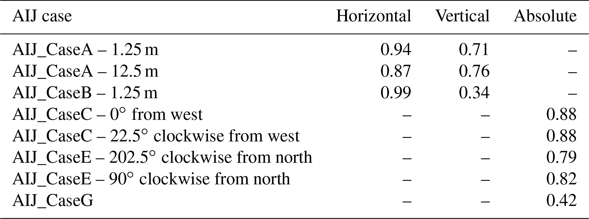
QUIC-URB and URock show good agreement for most of the cases. Two cases have a particularly low correlation coefficient: case G and the vertical wind speed for case B. For the first case, the low score is primarily due to the fact that in this case, the spatial variations of the wind speed are very low (thus even a small difference leads to a considerable decrease in the correlation). For the latter case, the low score is mainly explained by three points having high values in QUIC but low in URock. However, these points are not relevant since they are associated with upward winds in both QUIC and URock but downward winds in the AIJ data (see further discussion in Sect. 4.4).

In the next sections, QUIC-URB results are only shown when they differ significantly from URock results. Thus, most successes and limitations that are shown for URock are also applicable for QUIC-URB.

4.3 Isolated building – square base

The building used for this case has a square base of size b, and its height is twice its width ($h=\mathrm{2}\cdot b$). More information about the inflow wind profile and exact sensor location can be found in the case A description on the AIJ website and also in Meng and Hibi (1998).

Horizontal wind vectors near the ground show good agreement between models and observations. The main differences can be observed near the corner of the upwind facade where the cross-wind component is higher in the AIJ data than in URock. Absolute horizontal wind speed generally agrees except in an along-wind ellipse located right beside the building edge (red ellipse Fig. 17a). Due to the absence of a Röckle zone in this area, URock overestimates the wind speed (Fig. 17c).

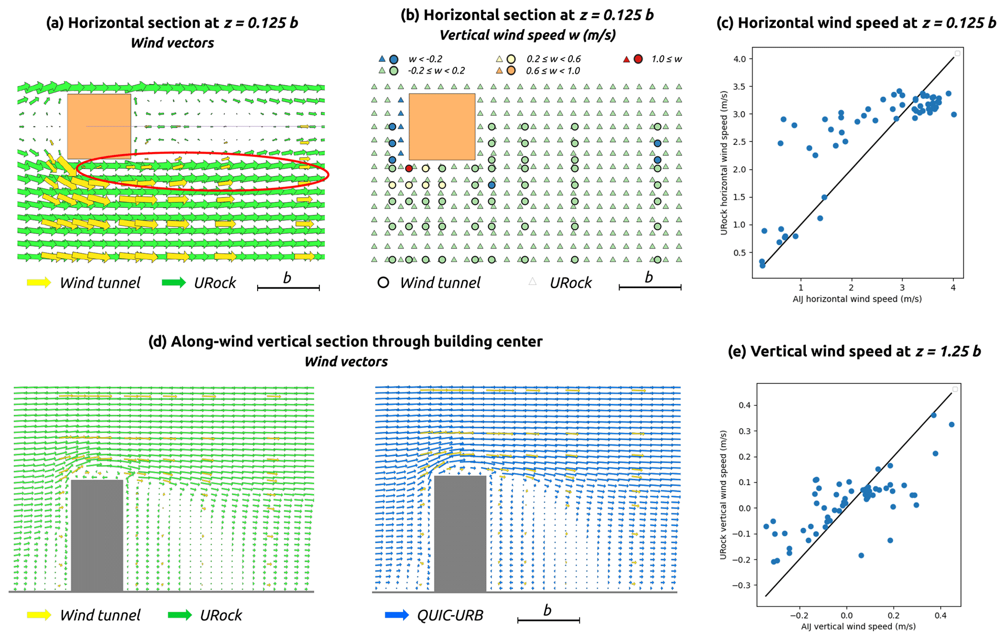
Figure 17 AIJ wind tunnel measurement as well as URock and QUIC-URB outputs for a square-base isolated building.

Near the ground ($z=\mathrm{0.125}\cdot b$), URock vertical wind speed values are low (remaining between −0.15 and 0.05 m s⁻¹), while observations show a higher wind speed range (from −0.5 to 1.5 m s⁻¹). The main spatial difference is located near the upwind edges of the building: the displacement vortex that goes cross-wind along the upwind facade is known to continue its way up and along-wind when it reaches the building corner. This leads to a non-negligible vertical component in this area as we can see in Fig. 17b.

At a higher level ($z=\mathrm{1.25}\cdot b$), the absolute vertical wind values observed are lower (below 0.5 m s⁻¹), and URock captures the spatial variability of the AIJ values well (Fig. 17e).

Wind tunnel measurements have also been performed within an along-wind sectional plane located on the building center. The wind vectors in URock and QUIC-URB are quite consistent with those observed in the AIJ data. The main difference is located at the top of the roof where a clear vortex structure is created in URock, while it does not exist (or is limited in size) in the wind tunnel observation and in QUIC-URB (Fig. 17d).

4.4 Isolated building – rectangular base

The building used for this case has a rectangular base of width b (along-wind) and length equal to 4⋅b (cross-wind), while its height is also 4⋅b. More information about the inflow wind profile and exact sensor location can be found in the case B description on the AIJ website.

The URock model has the same qualities and shortcomings for the rectangular as for the square-base case, except that the following shortcomings are exacerbated. First, the cross-wind component of the AIJ vectors near the building corner is higher than the along-wind one. This affects the wind direction of most wind vectors downstream (Fig. 18a). Second, the ellipse-shaped area impacted by wind speed overestimation is slightly wider than previously.

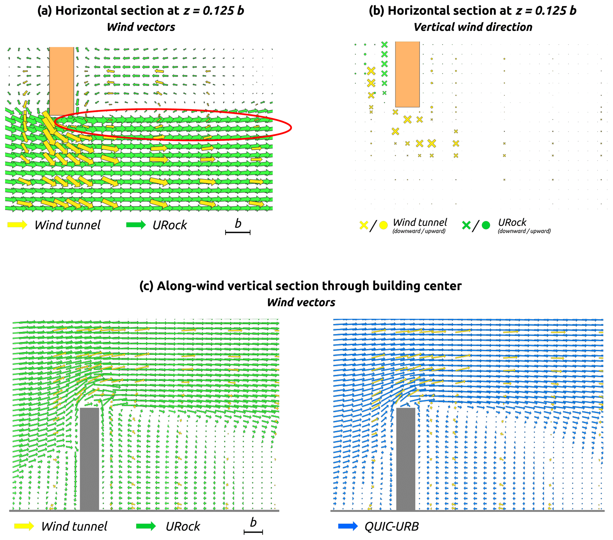
Figure 18 AIJ wind tunnel measurement as well as URock and QUIC-URB outputs for a rectangular-base isolated building.

One of the reasons for having low values for the cross-wind component near the building corner might come from the underestimation of downward wind in the displacement zone. In QUIC-URB and URock, a vortex is initialized in front of the upwind facade. This results in a downward wind close to the wall and an upward wind more upwind. According to Fig. 18b, it seems that this zone is either not relevant, or it has to be modified in order to have a downward wind where it currently has an upward wind.

The sectional plot shows a clear wind speed decrease in the AIJ measurement above the building cavity zone (in the rooftop zone and its prolongation; red ellipse in Fig. 18c). This zone does not correspond to any Röckle zone. Thus, it is overestimated by the URock model and also by QUIC-URB. In the square and rectangular building cases, the displacement zones differ between URock and QUIC-URB: they are bigger in URock. While it does not impact the wind field much in the square building case (Fig. 17d), the differences are more pronounced in the rectangular case: the wind speed and direction near the ground are more consistent between URock and the AIJ data than between QUIC-URB and the AIJ data (Fig. 18c).

4.5 Regularly distributed cubes

The nine cubic buildings used in this case are regularly distributed in a 3×3 layout. The distance separating each building is equal to the building width. More information about the inflow wind profile and exact sensor location can be found in the case C description on the AIJ website. Note that for this experiment, only the absolute wind speed is measured.

When the wind comes from the west, the scatterplot of URock versus AIJ wind speed looks quite similar to the one obtained for a single isolated building (Fig. 17c): half of the points follow the green regression line that is parallel to the identity line, and the other half are above this line (Fig. 19b). Most of the points located above the line belong to the area indicated by red ellipses drawn in Fig. 19a. A reduction of the wind speed in these zones may then have a double positive impact: first the points have a good chance to get closer to the green line, and second a reduction of the wind speed at the entrance of the streets may decrease the wind speed of all locations, thus decreasing the positive bias of the current URock version.

Figure 19 AIJ wind tunnel measurement and URock outputs for regularly distributed cubes.

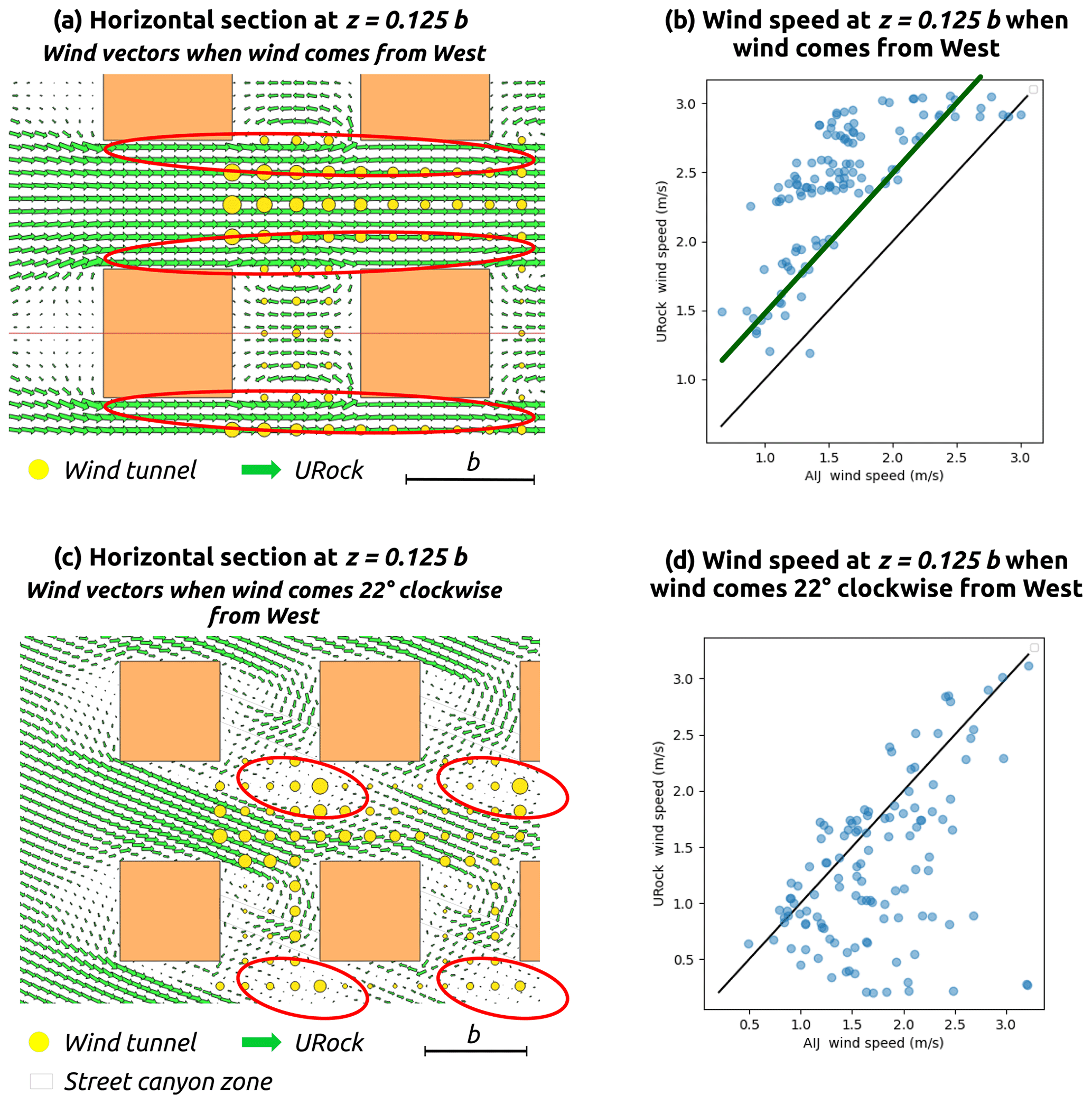
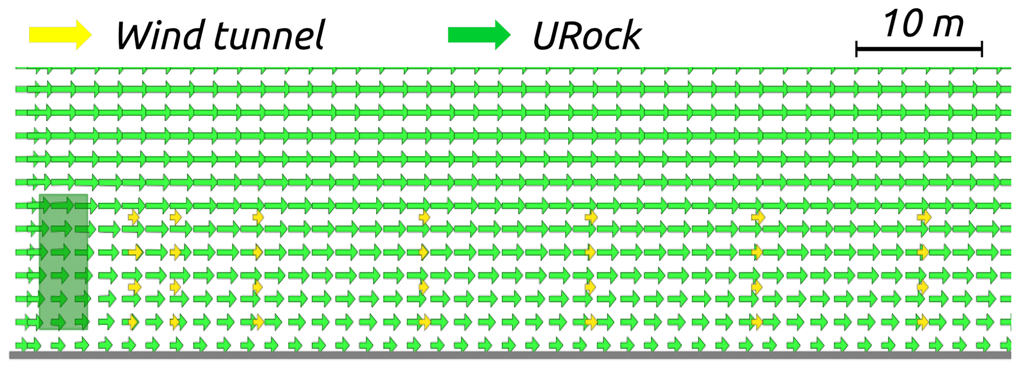
Figure 20 Wind vectors in an along-wind sectional plane located on the tree center: comparison between URock and AIJ wind tunnel measurement.

When the wind comes 22.5^∘ clockwise from the west, a large fraction of the domain has good agreement between URock output and observations (Fig. 19d). However, a non-negligible fraction of points are clearly underestimated by URock. The largest discrepancies are located downwind to most buildings, at the boundary between their cavity and wake zones (Fig. 19c). These underestimated zones are also downstream of a small set of street canyon zones. The superimposition of these zones results in a really small wind speed at the initialization stage (cavity–wake zone boundary), without any rationale to reach higher wind speeds after the mass balance stage since the wind emanating from the street canyon zones largely avoids the area indicated by red ellipses.

4.6 Isolated tree

The tree used for this case has a 2 m width square base; its crown starts from 1.2 m above ground level and extends up to 7 m. Its trunk is considered to have a negligible effect, and thus it is not represented in URock. More information about the inflow wind profile and exact sensor location can be found in the case G description on the AIJ website.

In URock, a single isolated tree induces only a really small decrease in the downward wind speed. On the contrary, the AIJ wind tunnel data show a considerable decrease: at 3 m height, the wind speed is reduced to about half of its initial value between 10 and 40 m downstream of the tree (Fig. 20). The same level of magnitude is obtained by Li et al. (2023) when simulating via a CFD model the wind around a 3.6 m wide, 3.6 m long, and 5 m tall tree canopy. Recently, Margairaz et al. (2022) updated the QES-Winds vegetation model for isolated trees. They replaced the initial QUIC-URB vegetation model by a new one that has a wake zone downwind of the tree. This model seems to show much better performance than the initial one. Further wind tunnel measurements or observations are needed to confirm this result, but it seems that the vegetation zone model used in URock and QUIC-URB is not appropriate for isolated trees and needs to be updated.

4.7 Real urban setting

The real urban setting used is a large city block with compact low-rise buildings. The wind tunnel observations are available for two cases: a potential future urban setting with three new high-rise buildings located on three existing large courtyards and the current urban setting with only the existing low-rise buildings. The first case has been chosen for URock evaluation. More information about the location and size of the buildings, the inflow wind profile, and the exact sensor location can be found in the case E description on the AIJ website or in Tominaga et al. (2004). Note that for this experiment, only the absolute wind speed is available.

When the wind comes from the east, the correlation between URock and AIJ wind speed is quite good. The points on the scatterplot are rather close to the identity line, although they are located slightly below it (Fig. 21b). About 10 % of the values are outliers: the majority of them are overestimations (yellow triangles) and three points are underestimations (yellow diamond). Most of these points are located in the largest street running in the east-northeast direction (Fig. 21a). Overestimation occurs on the northern part of the street, while the underestimations are located at the intersection with the courtyard where the highest building (60 m high) is located.

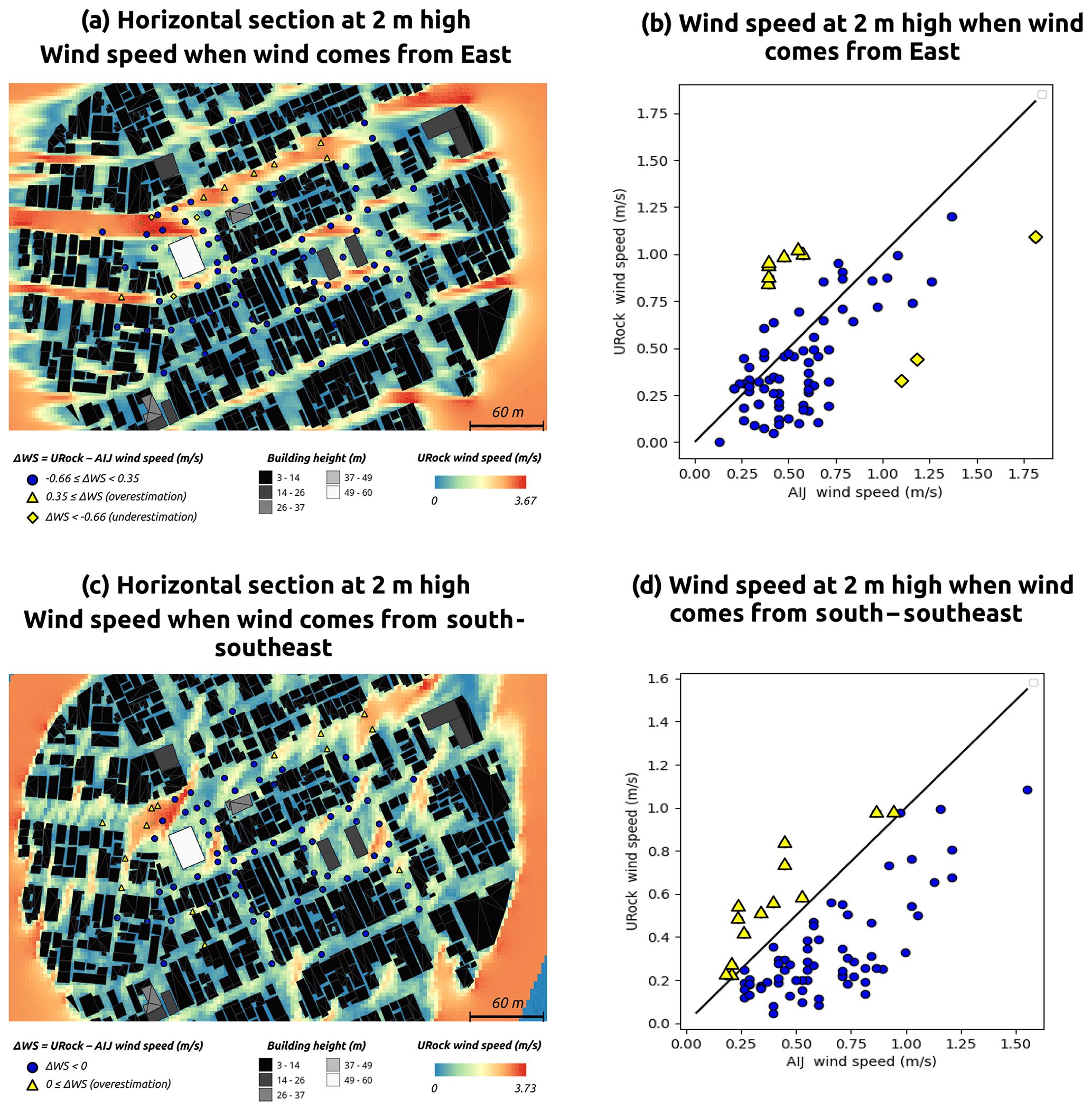
Figure 21 Comparison between URock outputs and AIJ wind tunnel measurement for a real urban setting at 2 m high.

When the wind comes from the south-southwest direction, the correlation between URock and AIJ wind speed is also good. There is a more pronounced underestimation of the wind speed, which is quite similar for all AIJ wind speeds (Fig. 21d). Almost 20 % of the values are outliers (yellow triangles). All of them are overestimations, and most of them are located far from high-rise buildings (Fig. 21c). Most of them are also outside any building influence (quite far downwind from any building), even though it is not the case for all locations. The central part of the zone, equipped with wind sensors, is not influenced by these outliers. Thus, the spatial variations in the zone of interest are quite well reproduced by URock, even though there is a general underestimation.

5 Conclusion and discussion

Most models dedicated to the calculation of wind speed in urban settings are intended for specialists, are computationally intensive, or are implemented in proprietary software. The model presented in this paper (URock 2023a) is available in the free and open-source QGIS software in the UMEP plug-in. Its method is based on the so-called Röckle approach: first, the wind field near obstacles is initialized according to empirical rules drawn from wind tunnel observations, and second, the airflow is balanced, minimizing the modification of the initial wind field. This method is reputed to be quick, but to our knowledge, only proprietary implementations exist. The URock 2023a model is based on the Röckle zones implemented in the state-of-the-art QUIC-URB software. The model methods and implementations are described in Sects. 2 and 3, respectively. The evaluation is performed using both wind tunnel measurement (from the AIJ) and QUIC-URB outputs. This is a good opportunity to show that the results obtained with URock are (i) very close to the ones obtained using QUIC-URB, (ii) close to the ones obtained by the wind tunnel experiments for most cases, and (iii) open to improvements in some cases (as described below).

In the isolated building cases (Sect. 4.3, 4.4), the wind speeds above the building and downstream do not perfectly fit the wind tunnel data. In the square-base case, it seems that the rooftop perpendicular zone is too tall, while in the rectangular-base case, it seems that the rooftop perpendicular zone should extend not only above the roof but also above the cavity zone (Fig. 18c). Currently, a rooftop zone ends when the roof ends, even though the initial zone length is longer. A potential improvement could be to keep the rooftop zone, even though it is wider (along-wind) than the building width.

In the third case, when the wind comes from 22.5^∘ clockwise from the left, small street canyons are created. The wind direction in these zones might not be accurate, which might be partially responsible for the nearby wind speed underestimations. In this configuration, where the street canyon concept is not quite applicable due to a very limited street canyon length, the wind flow should be modified in order not to have a drastic change in wind direction. Wind tunnel experiments, where the effect of the length of the street canyon is investigated, could be a good dataset for model improvements.

In the first three cases (Sect. 4.3, 4.4, and 4.5), the agreement between the URock field and the wind tunnel data is quite good. Most of the differences observed might be attributed to the high wind speed values located in the along-wind ellipse-shaped area starting from the upwind corner of the building. This zone is not defined as a Röckle zone, although decreasing the wind speed here during the initialization stage could solve most of the problems as a result of the mass balance process:

• reduction of the final wind speed in this zone (Fig. 17),

• increase in the cross-wind component near the upwind corner (Fig. 17a),

• increase in the vertical component near the upwind corner (Fig. 17),

• decrease in the global flow rate entering the streets and thus a reduction in the wind speed in most locations (Fig. 19a).

As a first attempt, a solution could also be to only delete the displacement vortex zone or set a downward wind in the displacement zone. Indeed, the analysis of the rectangular-base case (B) showed that both URock and QUIC-URB have an upward wind where AIJ data show downward wind. This change may lead to modification in the upstream wind, even though we do not expect it to solve all the problems.

The isolated tree case does not show good agreement with the wind tunnel data. It should be further verified using additional wind tunnel or observation data, and the Röckle vegetation zones should be modified if necessary.

There is a general wind speed underestimation when URock is compared with a compact urban setting. Similar results have been identified in a previous work by Girard et al. (2018). It seems that this behavior is exacerbated when the number of upstream buildings increases (direction SSW compared to E). While it seems that the spatial variations are quite well reproduced, investigations could be carried out to solve this limitation: the vertical wind profile could be updated to take into account the morphometric characteristics of the urban setting.

Outside these model improvements, the model is currently limited to flat areas. A future version will account for complex terrains, taking into account the latest literature in the field (e.g., that of Robinson et al., 2023).

Appendix A: Calculate building Röckle zones

This section contains more details about some of the building Röckle zones as calculated in URock.

A1 Displacement zone

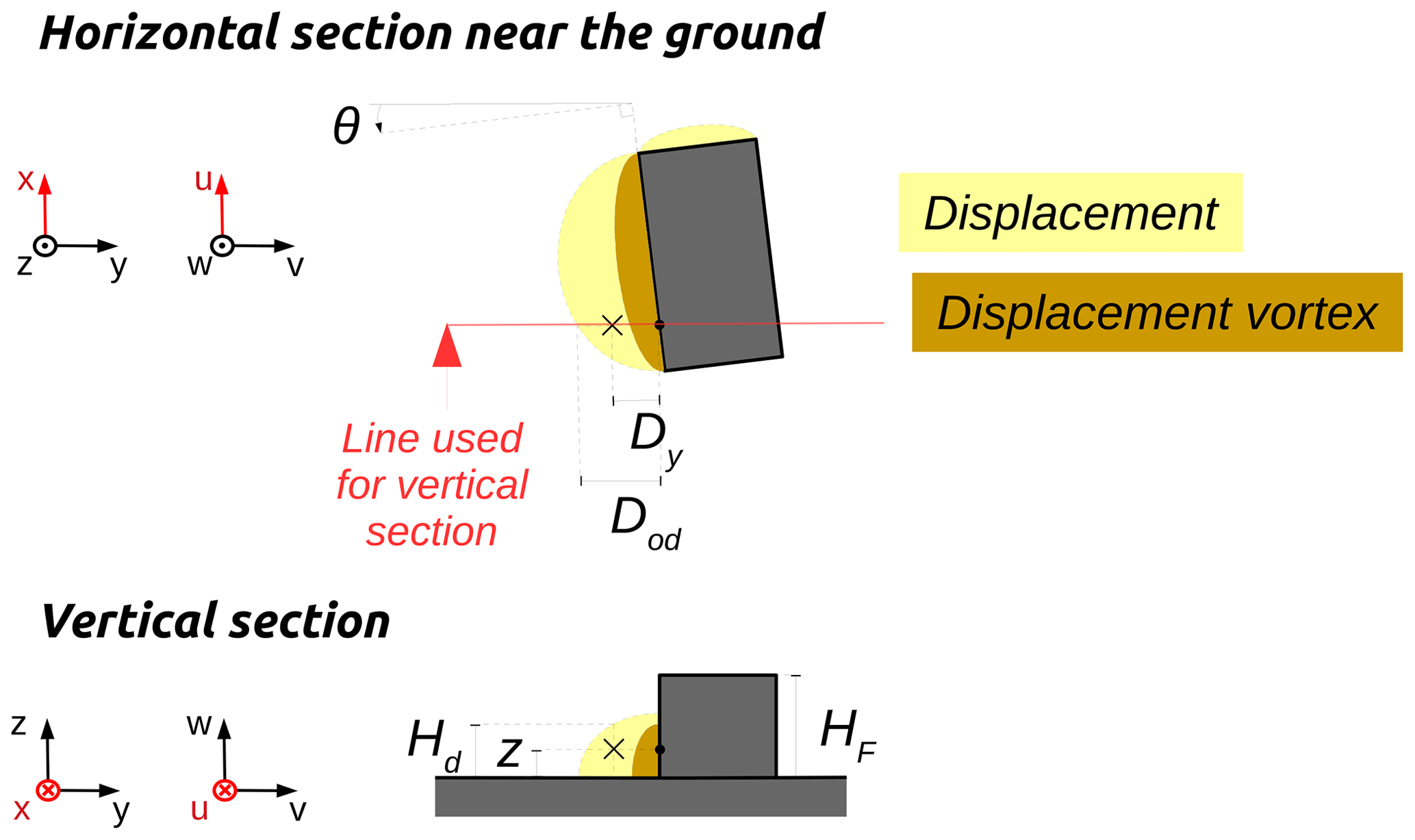
The displacement zone is defined as a quarter of an ellipse located on each upwind facade (see Fig. 1a). The radius of the ellipse along the facade direction is half the facade length, the radius along the axis perpendicular to the facade (L_f) is defined by Eq. (A1), and the vertical radius is 60 % of the upwind facade height (H_F) (Kaplan and Dinar, 1996).

$$\begin{array}{}\text{(A1)}& L_{\mathrm{f}}=\mathrm{1.5}\cdot {\displaystyle \frac{W_{\mathrm{eff}}}{\mathrm{1}+\mathrm{0.8}\cdot \frac{W_{\mathrm{eff}}}{H_{\mathrm{F}}}}}\end{array}$$

A2 Displacement vortex zone

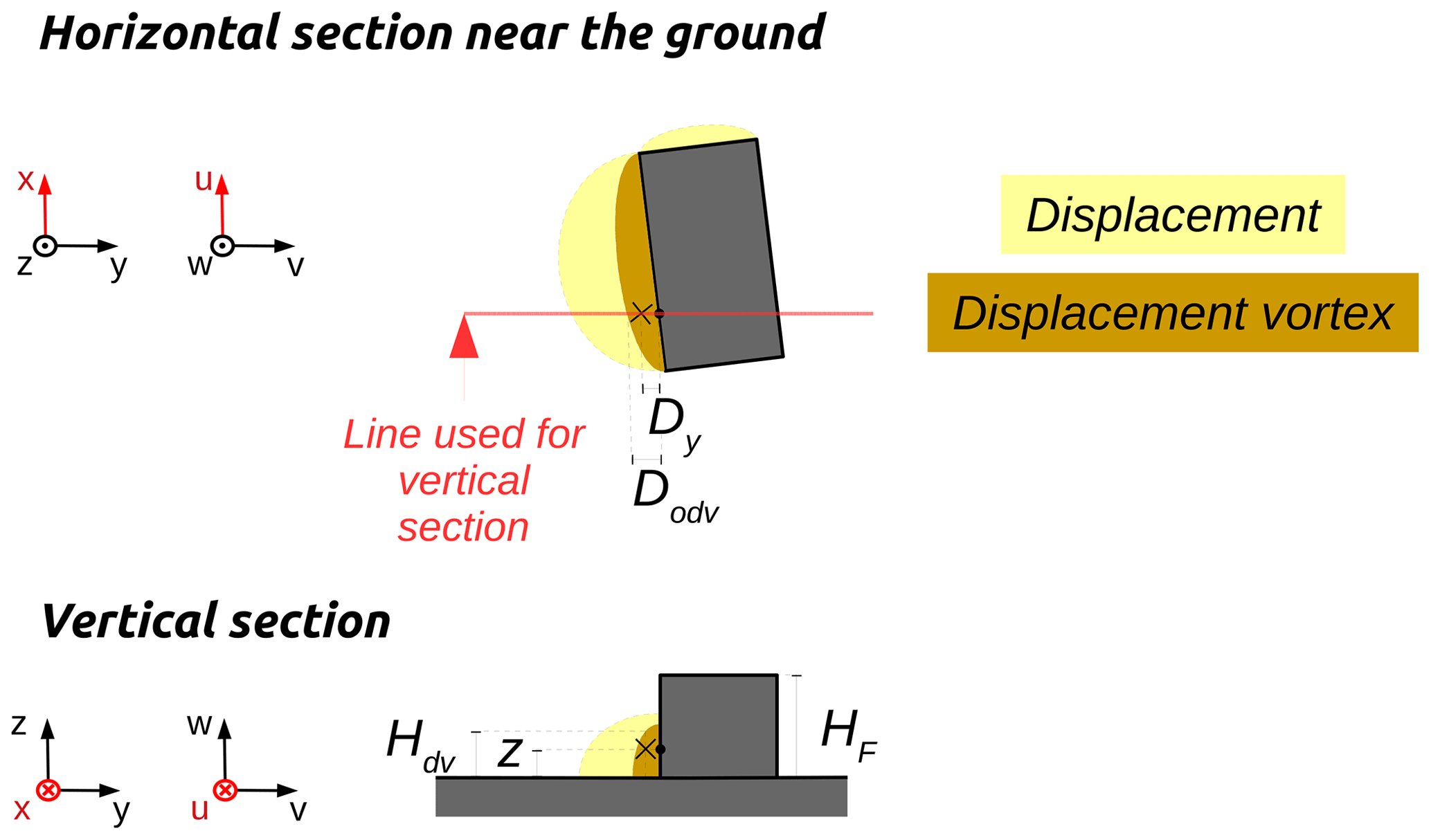
The displacement vortex zone is defined as a quarter of an ellipse located on each upwind facade whenever the angle between the wind direction and an upwind facade ${\mathit{\theta }}_{\mathrm{wind}/{\mathrm{upwind}}_{\mathrm{F}}}$ is within [90-PERPENDICULAR_THRESHOLD_ANGLE, 90+PERPENDICULAR_THRESHOLD_ANGLE] (see Fig. 1a). The size of the zone is identical in URock and QUIC-URB: the radius of the ellipse along the facade direction is half the facade length, the radius along the axis perpendicular to the facade (L_fv) is defined by Eq. (A2), and the vertical radius is 50 % of the upwind facade height (H_F) (Bagal et al., 2004).

$$\begin{array}{}\text{(A2)}& L_{\mathrm{fv}}=\mathrm{0.6}\cdot {\displaystyle \frac{W_{\mathrm{eff}}}{\mathrm{1}+\mathrm{0.8}\cdot \frac{W_{\mathrm{eff}}}{H_{\mathrm{F}}}}}\end{array}$$

A3 Cavity zone

The cavity zone can be seen as a quarter of an ellipse but having a slightly modified equation. If a standard ellipse has a fixed center, the one used in URock has a center which moves upon the along-wind direction, following the facade coordinates (see Fig. 1a). Equation (A3) gives the modified ellipse coordinates for a wind parallel to the y axis (in URock, all geometries are rotated in order to have wind coming along the y axis – see Sect. 2.1.2):

$$\begin{array}{}\text{(A3)}& {\displaystyle \frac{x^{\mathrm{2}}}{W_{\mathrm{BBox}}^{\mathrm{2}}}}+{\displaystyle \frac{(y-y_{{\mathrm{0}}_{\mathrm{F}}}(x){)}^{\mathrm{2}}}{L_{\mathrm{r}}^{\mathrm{2}}}}+{\displaystyle \frac{z^{\mathrm{2}}}{H_{\mathrm{F}}^{\mathrm{2}}}}=\mathrm{1},\end{array}$$

where x is the coordinate of the ellipse along the x axis, W_BBox the radius of the ellipse along x (corresponding to the cross-wind width of the stacked block), y the coordinate of the ellipse along the y axis, $y_{{\mathrm{0}}_{\mathrm{F}}}\left(x\right)$ the y coordinate of the facade (may vary along the x axis), L_r the radius of the ellipse along y as defined by Eq. (A4), z the coordinate of the ellipse along the z axis, and H_F the radius of the ellipse along z (corresponding to the facade height).

$$\begin{array}{}\text{(A4)}& L_{\mathrm{r}}=\mathrm{1.8}\cdot {\displaystyle \frac{W_{\mathrm{eff}}}{{\left(\frac{L_{\mathrm{eff}}}{H}\right)}^{\mathrm{0.3}}\cdot \left(\mathrm{1}+\mathrm{0.24}\cdot \frac{L_{\mathrm{eff}}}{H}\right)}}\end{array}$$

A4 Rooftop perpendicular zone

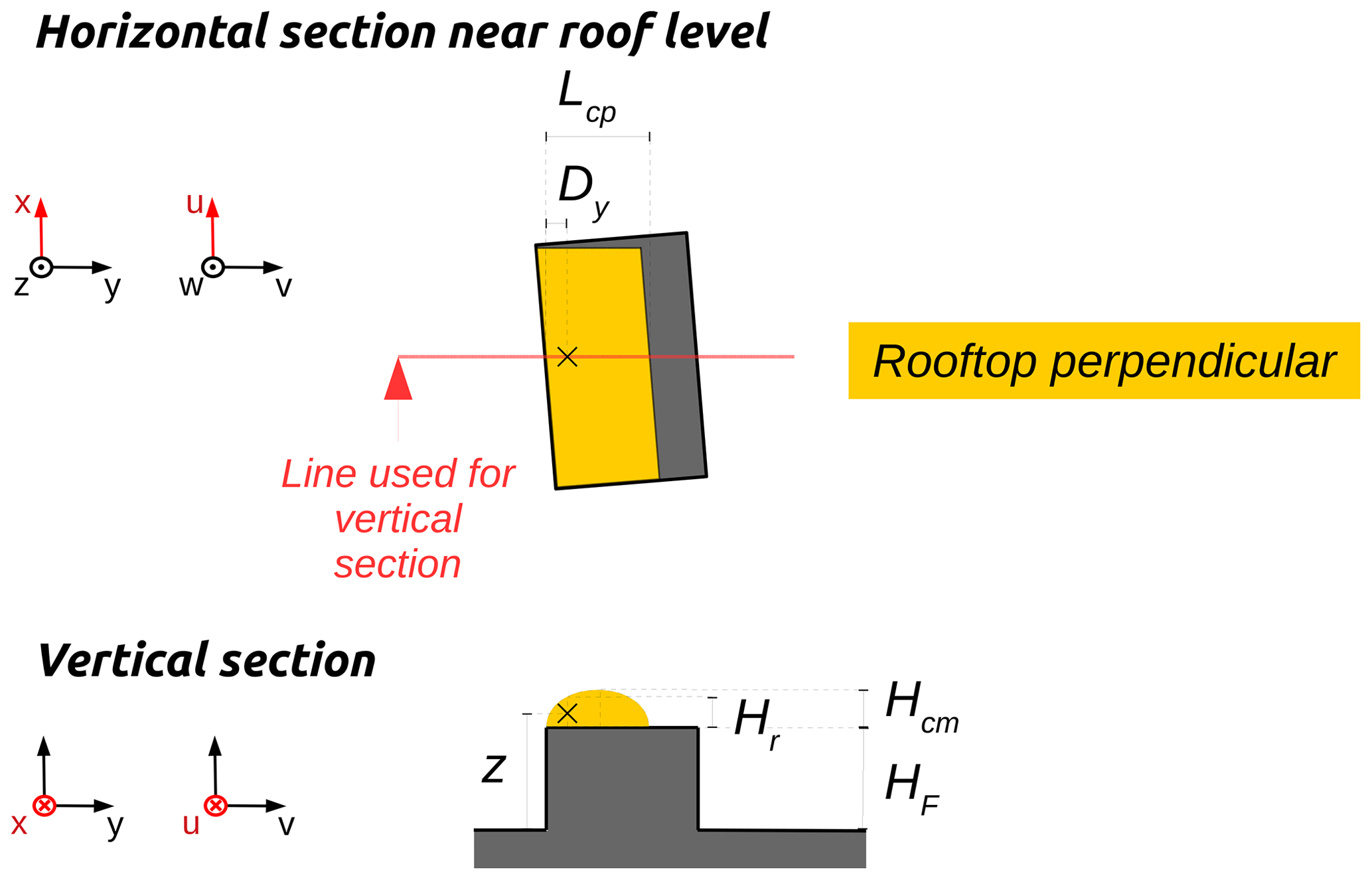
The rooftop perpendicular zone is defined as a half-ellipse-base cylinder cut along its height and located on each rooftop. It is only created when the angle between the wind direction and an upwind facade ${\mathit{\theta }}_{\mathrm{wind}/{\mathrm{upwind}}_{\mathrm{F}}}$ is within [90-PERPENDICULAR_THRESHOLD_ANGLE, 90+PERPENDICULAR_THRESHOLD_ANGLE] (see Fig. 1a). The cylinder height is the length of the upwind facade; the vertical diameter H_cm and the diameter perpendicular to the upwind facade d_cp are respectively defined by Eqs. (A5) and (A6) (Pol et al., 2006).

$$\begin{array}{}\text{(A5)}& \begin{array}{rl}{H}_{\mathrm{cm}}& =\mathrm{0.22}\cdot (\mathrm{0.67}\times \mathrm{MIN}(H_{\mathrm{F}},W_{\mathrm{eff}})+\mathrm{0.33}\\ & \cdot \mathrm{MAX}(H_{\mathrm{F}},W_{\mathrm{eff}}))\end{array}\end{array}$$

$$\begin{array}{}\text{(A6)}& {\displaystyle }\left\{\begin{array}{ll}{d}_{\mathrm{cp}}& =L_{\mathrm{cp}}\cdot \sin \left({\mathit{\theta }}_{\mathrm{wind}/{\mathrm{upwind}}_{\mathrm{F}}}\right)\\ L_{\mathrm{cp}}& =\mathrm{0.9}\cdot (\mathrm{0.67}\times \mathrm{MIN}(H_{\mathrm{F}},W_{\mathrm{eff}})+\mathrm{0.33}\\ & \cdot \mathrm{MAX}(H_{\mathrm{F}},W_{\mathrm{eff}}))\end{array}\right.\end{array}$$

A5 Rooftop corner zone

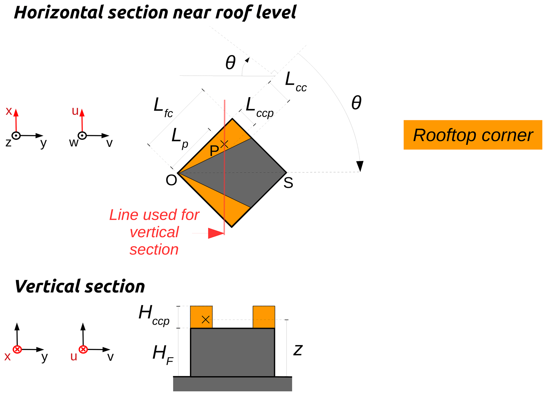
The rooftop corner zone is defined as a square-base oblique pyramid located on a rooftop along an upwind facade with the apex starting from the most upwind point (see Fig. 1a). The pyramid height is equal to the length of the upwind facade (L_fc), while the width of the pyramid base (L_cc) is defined by Eq. (A7) (Bagal et al., 2004):

$$\begin{array}{}\text{(A7)}& \begin{array}{rl}{L}_{\mathrm{cc}}& =\mathrm{2}\cdot L_{\mathrm{fc}}\cdot \tan (\mathrm{2.94}\cdot \exp \left(\mathrm{0.0297}\cdot \left(\left|{\mathit{\theta }}_{\mathrm{wind}/{\mathrm{upwind}}_{\mathrm{F}}}\right|\right.\right.\\ & \left.\left.-{\displaystyle \frac{\mathit{\pi }}{\mathrm{2}}}\right)\right),\end{array}\end{array}$$

where ${\mathit{\theta }}_{\mathrm{wind}/{\mathrm{upwind}}_{\mathrm{F}}}$ is the angle between the wind direction and an upwind facade (in radians).

Appendix B: Calculation of wind factors

Wind factors along the three components are defined as a fraction of the wind speed at a given height and position and are Röckle-zone-dependent. In this section, the equations used to calculate these wind factors are described. For a more visual representation of these equations, please refer to the wind field illustrated in Fig. 1.

B1 Displacement zone

In the displacement zone, the wind factors are defined according to Eq. (B1), where z<H_d (Bagal et al., 2004).

$$\begin{array}{}\text{(B1)}& {\displaystyle }\left\{\begin{array}{l}\frac{V_{\mathrm{0}}\left(z\right)}{V_p\left(H_{\mathrm{F}}\right)}=\frac{U_{\mathrm{0}}\left(z\right)}{V_p\left(H_{\mathrm{F}}\right)}=C_{\mathrm{d}z}\cdot (\frac{z}{H_{\mathrm{F}}}{)}^p\\ H_{\mathrm{d}}=\mathrm{0.6}\cdot H_{\mathrm{F}}\cdot \sqrt{\left(\mathrm{1}-\frac{D_y^{\mathrm{2}}}{D_{\mathrm{od}}^{\mathrm{2}}}\right)}\end{array}\right.\end{array}$$

Here (see Fig. B1), D_y is the distance to the wall along the y axis, H_d is the ellipsoid height at the distance D_y, C_dz=0.4, p=0.16, z is the level of the cell, D_od is the length of the ellipsoid along the y axis at z=0 m, θ is the angle between the wind direction and perpendicular to the building wall, and H_F is the building facade height.

Figure B1 Variables needed for wind factor calculation in displacement zones.

B2 Displacement vortex zone

In the vortex zone, the wind factors are defined according to Eq. (B2), where z<H_dv (Bagal et al., 2004).

$$\begin{array}{}\text{(B2)}& {\displaystyle }\left\{\begin{array}{l}\frac{V_{\mathrm{0}}\left(z\right)}{V_p\left(H_{\mathrm{F}}\right)}=-\left[\mathrm{0.6}\cdot \cos \left(\frac{\mathit{\pi }\cdot z}{\mathrm{0.5}\cdot H_{\mathrm{F}}}\right)+\mathrm{0.05}\right]\cdot \mathrm{0.6}\cdot \sin \left(\frac{\mathit{\pi }\cdot D_y}{D_{\mathrm{odv}}}\right)\\ \frac{W_{\mathrm{0}}\left(z\right)}{V_p\left(H_{\mathrm{F}}\right)}=-\left[\mathrm{0.1}\cdot \cos \left(\frac{\mathit{\pi }\cdot D_y}{D_{\mathrm{odv}}}\right)+\mathrm{0.05}\right]\\ H_{\mathrm{dv}}=\mathrm{0.5}\cdot H_{\mathrm{F}}\cdot \sqrt{\left(\mathrm{1}-\frac{D_y^{\mathrm{2}}}{D_{\mathrm{odv}}^{\mathrm{2}}}\right)}\end{array}\right.\end{array}$$

Here (see Fig. B2), Dy is the distance to the wall along the y axis, H_dv is the ellipsoid height at the distance D_y, C_dz=0.4, p=0.16, z is the level of the cell, D_od is the length of the ellipsoid along the y axis at z=0 m, θ is the angle between the wind direction and perpendicular to the building wall, and H_F is the building facade height.

Figure B2 Variables needed for wind factor calculation in displacement vortex zones.

B3 Cavity zone

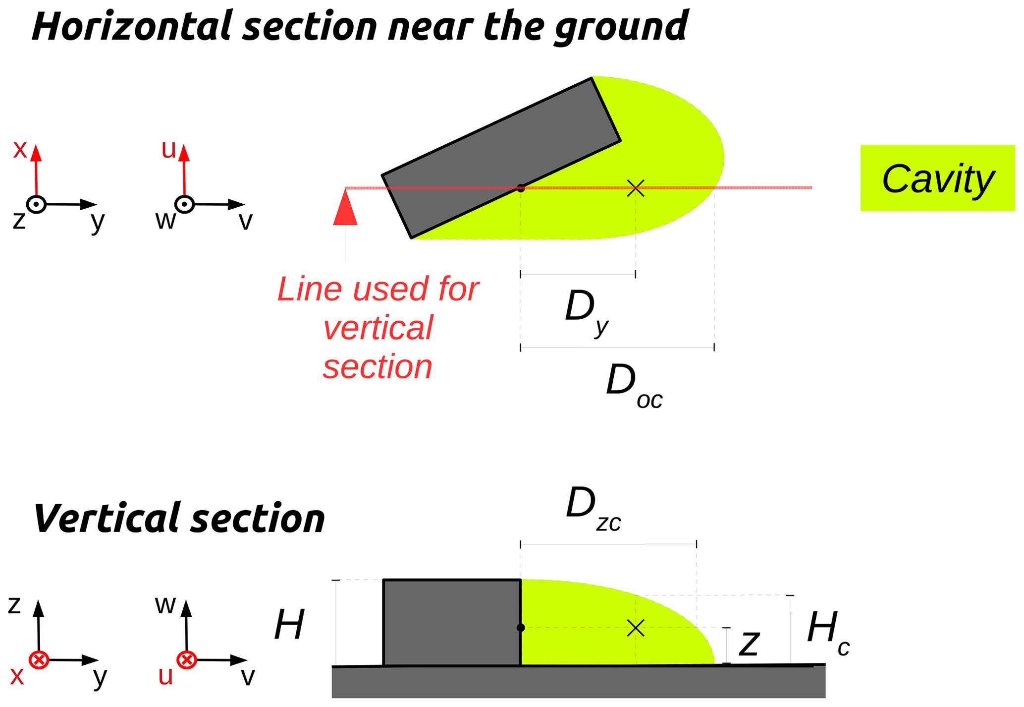
In the cavity zone, the wind factors are defined according to Eq. (B3), where z<H_c (Kaplan and Dinar, 1996).

$$\begin{array}{}\text{(B3)}& {\displaystyle }\left\{\begin{array}{l}\frac{V_{\mathrm{0}}(D_y,z)}{V_p\left(H\right)}=-{\left(\mathrm{1}-\frac{D_y}{D_{\mathrm{oc}}\sqrt{\mathrm{1}-\frac{z^{\mathrm{2}}}{H^{\mathrm{2}}}}}\right)}^{\mathrm{2}}\\ H_c=H\cdot \sqrt{\mathrm{1}-\frac{D_y^{\mathrm{2}}}{D_{\mathrm{oc}}^{\mathrm{2}}}}\end{array}\right.\end{array}$$

Here (see Fig. B3), D_y is the distance to the wall along the y axis, H_c is the ellipsoid height at the distance D_y, z is the level of the cell, D_oc is the length of ellipsoid along the y axis at z=0 m, and H is the stacked block height.

Figure B3 Variables needed for wind factor calculation in cavity zones.

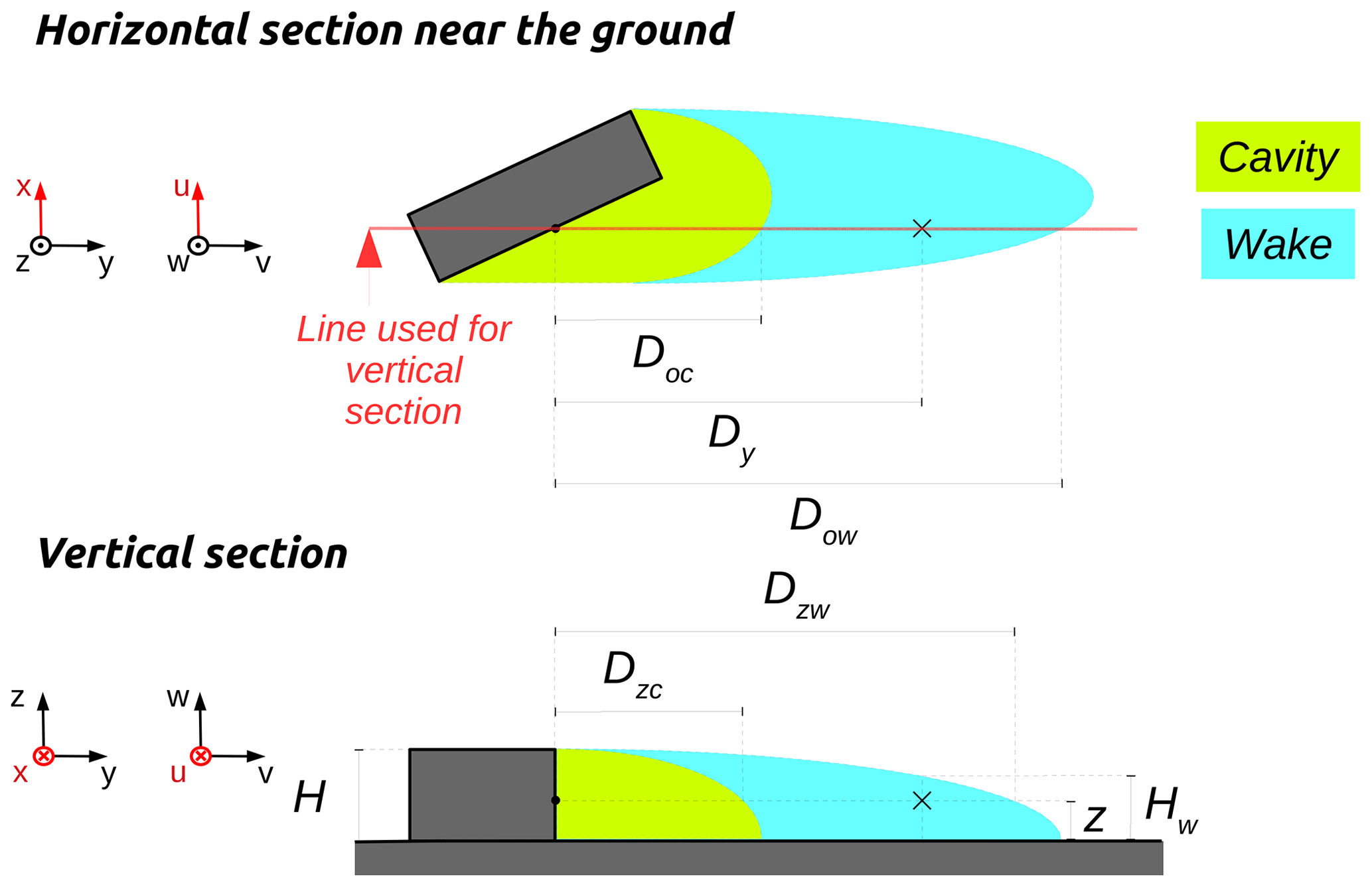
B4 Wake zone

In the vortex zone, the wind factors are defined according to Eq. (B4), where z<H_w (Kaplan and Dinar, 1996).

$$\begin{array}{}\text{(B4)}& {\displaystyle }\left\{\begin{array}{l}\frac{V_{\mathrm{0}}(D_y,z)}{V_p\left(z\right)}=-\left[\mathrm{1}-{\left(\frac{D_{\mathrm{oc}}}{D_y}\right)}^{\mathrm{1.5}}{\sqrt{\mathrm{1}-\frac{z^{\mathrm{2}}}{H^{\mathrm{2}}}}}^{\mathrm{1.5}}\right]\\ H_w=H\cdot \sqrt{\mathrm{1}-\frac{D_y^{\mathrm{2}}}{D_{\mathrm{ow}}^{\mathrm{2}}}}\end{array}\right.\end{array}$$

Here (see Fig. B4), D_y is the distance to the wall along the y axis, H_w is the ellipsoid height at the distance D_y, z is the level of the cell, D_ow is the length of the ellipsoid along the y axis at z=0 m, and H is the stacked block height.

Figure B4 Variables needed for wind factor calculation in wake zones.

B5 Rooftop perpendicular zone

In the vortex zone, the wind factors are defined according to Eq. (B5), where $H<z<H+H_{\mathrm{r}}$ (Pol et al., 2006).

$$\begin{array}{}\text{(B5)}& {\displaystyle }\left\{\begin{array}{l}\frac{V_{\mathrm{0}}(D_y,z)}{V_p\left(z_{\mathrm{ref}}\right)}=-{\left(\frac{H+H_{\mathrm{r}}-z}{z_{\mathrm{ref}}}\right)}^p\cdot \left|\frac{H+H_{\mathrm{r}}-z}{H_{\mathrm{r}}}\right|\\ H_{\mathrm{r}}=H_{\mathrm{cm}}\cdot \sqrt{\mathrm{1}-{\left(\frac{D_y-\frac{L_{\mathrm{cp}}}{\mathrm{2}}}{L_{\mathrm{cp}}}\right)}^{\mathrm{2}}}\end{array}\right.\end{array}$$

Here (see Fig. B5), p=0.16, V(z_ref) is the wind speed at measurement height z_ref, D_y is the distance to the wall along the y axis, H_r is the ellipsoid height at the distance D_y, H_cm is the maximum ellipsoid height, L_cp is the rooftop perpendicular length, z is the level of the cell, and H is the facade height.

Figure B5 Variables needed for wind factor calculation in rooftop perpendicular zones.

B6 Rooftop corner zone

In the vortex zone, the wind factors are defined according to Eq. (B6), where $H<z<H+H_{\mathrm{ccp}}$ (Pol et al., 2006).

$$\begin{array}{}\text{(B6)}& {\displaystyle }\left\{\begin{array}{l}\frac{U_{\mathrm{0}}(D_y,z)}{V_p\left(z_{\mathrm{ref}}\right)}=-C\mathrm{1}\cdot {\left(\frac{H+H_{\mathrm{ccp}}-z}{z_{\mathrm{ref}}}\right)}^p\cdot \left|\frac{H+H_{\mathrm{ccp}}-z}{H_{\mathrm{ccp}}}\right|\cdot \sin (\mathrm{2}\cdot \mathrm{\Theta })\\ \frac{V_{\mathrm{0}}(D_y,z)}{V_p\left(z_{\mathrm{ref}}\right)}=-C\mathrm{1}\cdot {\left(\frac{H+H_{\mathrm{ccp}}-z}{z_{\mathrm{ref}}}\right)}^p\cdot \left|\frac{H+H_{\mathrm{ccp}}-z}{H_{\mathrm{ccp}}}\right|\cdot {\sin }^{\mathrm{2}}\mathrm{\Theta }\\ H_{\mathrm{ccp}}=L_{\mathrm{ccp}}=\frac{L_{\mathrm{cc}}\cdot \sqrt{x_{L_p}^{\mathrm{2}}+y_{L_p}^{\mathrm{2}}}}{L_{\mathrm{fc}}\cdot \cos (\mathrm{\Theta }-\widehat{SOP})}\\ C\mathrm{1}=\frac{\mathrm{1}+\mathrm{0.05}*W_{\mathrm{eff}}}{H_{\mathrm{F}}}\end{array}\right.\end{array}$$

Here (see Fig. B6), C1 is the wind speed factor, H_F is the facade height, W_eff is the stacked block effective length, V(z_ref) is the wind speed at measurement height z_ref, H_r is the ellipsoid height at the distance D_y, H_ccp is the H_ccx value for point p, L_ccp is the L_ccx value for point p, L_fc is the facade length, L_cc is the L_ccx value at the end of the facade length, $x_{L_{\mathrm{cp}}}$ and $y_{L_{\mathrm{cp}}}$ are the absolute coordinates of vector L_ccp, z is the level of the cell, θ is the angle between the wind direction and perpendicular to the building wall, and $\widehat{\mathrm{SOP}}$ is the angle between points S, O, and P.

Figure B6 Variables needed for wind factor calculation in rooftop corner zones.

B7 Street canyon zone

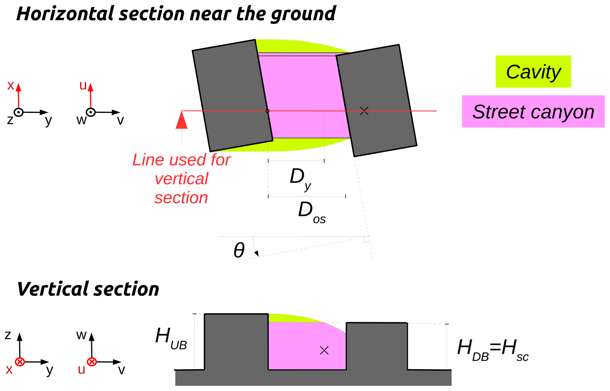
In the street canyon zone, the wind factors are defined according to Eq. (B7), where $H<z<H_{sc}$ and z<H_c (adapted from Kaplan and Dinar, 1996, and Singh et al., 2008).

$$\begin{array}{}\text{(B7)}& {\displaystyle }\left\{\begin{array}{l}\frac{U_{\mathrm{0}}\left(D_y\right)}{V_p\left(H_{\mathrm{UB}}\right)}=\sin (\mathrm{2}\cdot \mathrm{\Theta })\cdot \left[\mathrm{0.5}+\frac{D_y\cdot (D_{\mathrm{os}}-D_y}{\mathrm{0.5}\cdot D_{\mathrm{os}}^{\mathrm{2}}}\right]\\ \frac{V_{\mathrm{0}}\left(D_y\right)}{V_p\left(H_{\mathrm{UB}}\right)}={\sin }^{\mathrm{2}}\left(\mathrm{\Theta }\right)-{\cos }^{\mathrm{2}}\mathrm{\Theta }\cdot \left[\frac{D_y\cdot (D_{\mathrm{os}}-D_y)}{\mathrm{0.25}\cdot D_{\mathrm{os}}^{\mathrm{2}}}\right]\\ \frac{W_{\mathrm{0}}\left(D_y\right)}{V_p\left(H_{\mathrm{UB}}\right)}=-|\mathrm{0.5}\cdot \left(\mathrm{1}-\frac{D_y}{\mathrm{0.5}\cdot D_{\mathrm{os}}}\right)|\cdot \left(\mathrm{1}-\frac{D_{\mathrm{os}}}{\mathrm{0.5}\cdot D_{\mathrm{os}}}\right)\end{array}\right.\end{array}$$

Here (see Fig. B7), θ is the angle between the wind direction and perpendicular to the downwind building wall, D_y is the distance along the y axis from the upstream building wall, D_os is the distance between the upstream and the downwind buildings of the canyon, H_UB is the upwind building height, H_SC is the height of the lowest street canyon building, and H_c is the ellipsoid height at the distance D_y (Eq. B3).

Figure B7 Variables needed for wind factor calculation in street canyon zones.

B8 Vegetation in built-up areas

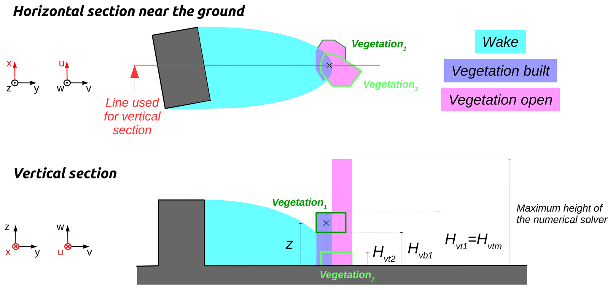
In the vegetation built zone, the wind factors are defined according to Eq. (B8), where z<H_vtm (Nelson et al., 2009).

$$\begin{array}{}\text{(B8)}& {\displaystyle \frac{V_{\mathrm{0}}\left(z\right)}{V_p\left(z\right)}}={\displaystyle \frac{\ln \left(\frac{H_{\mathrm{vtm}}}{z_{\mathrm{0}}}\right)}{\ln \left(\frac{z}{z_{\mathrm{0}}}\right)}}\cdot \exp \left({\mathit{\alpha }}_i\cdot \left({\displaystyle \frac{z}{H_{\mathrm{vtm}}}}-\mathrm{1}\right)\right)\end{array}$$

Here (see Fig. B8), H_vtm is the maximum canopy height above the cell of interest, z₀ is the roughness length of the surface, z is the level of the cell, and α_i is the attenuation factor of vegetation i (0 if there is no vegetation at height z).

Figure B8 Variables needed for wind factor calculation in vegetation built zones.

B9 Vegetation in open areas

In the vegetation open zone, the wind factors are defined according to Eq. (B9), where z<H_vtm, and to Eq. (B10), where z≥H_vtm (Nelson et al., 2009).

$$\begin{array}{}\text{(B9)}& {\displaystyle \frac{V_{\mathrm{0}}\left(z\right)}{V_p\left(z\right)}}={\displaystyle \frac{\ln \left(\frac{H_{\mathrm{vtm}}-d}{z_{\mathrm{0}}}\right)}{\ln \left(\frac{z}{z_{\mathrm{0}}}\right)}}\cdot \exp \left({\mathit{\alpha }}_i\cdot \left({\displaystyle \frac{z}{H_{\mathrm{vtm}}}}-\mathrm{1}\right)\right)\text{(B10)}& {\displaystyle \frac{V_{\mathrm{0}}\left(z\right)}{V_p\left(z\right)}}={\displaystyle \frac{\ln \left(\frac{z-d}{z_{\mathrm{0}}}\right)}{\ln \left(\frac{z}{z_{\mathrm{0}}}\right)}}\end{array}$$

Here (see Fig. B9), H_vtm is the maximum canopy height above the cell of interest, d is the displacement length (Table 1), z₀ is the roughness length of the surface, z is the level of the cell, and α_i is the attenuation factor of vegetation i (0 if there is no vegetation at height z).

Figure B9 Variables needed for wind factor calculation in vegetation open zones.