CMIP6 simulations with the compact Earth system model OSCAR v3.1

Reduced-complexity models, also called simple climate models or compact models, provide an alternative to Earth system models (ESMs) with lower computational costs, although at the expense of spatial and temporal information. It remains important to evaluate and validate these reduced-complexity models. Here, we evaluate a recent version (v3.1) of the OSCAR model using observations and results from ESMs from the current Coupled Model Intercomparison Project 6 (CMIP6). The results follow the same post-processing used for the contribution of OSCAR to the Reduced Complexity Model Intercomparison Project (RCMIP) Phase 2 regarding the identification of stable configurations and the use of observational constraints. These constraints succeed in decreasing the overestimation of global surface air temperature over 2000–2019 with reference to 1961–1900 from 0.60±0.11 to 0.55±0.04 K (the constraint being 0.54±0.05 K). The equilibrium climate sensitivity (ECS) of the unconstrained OSCAR is 3.17±0.63 K, while CMIP5 and CMIP6 models have ECSs of 3.2±0.7 and 3.7±1.1 K, respectively. Applying observational constraints to OSCAR reduces the ECS to 2.78±0.47 K. Overall, the model qualitatively reproduces the responses of complex ESMs, although some differences remain due to the impact of observational constraints on the weighting of parametrizations. Specific features of OSCAR also contribute to these differences, such as its fully interactive atmospheric chemistry and endogenous calculations of biomass burning, wetlands CH₄ and permafrost CH₄ and CO₂ emissions. Identified main points of needed improvements of the OSCAR model include a low sensitivity of the land carbon cycle to climate change, an instability of the ocean carbon cycle, the climate module that is seemingly too simple, and the climate feedback involving short-lived species that is too strong. Beyond providing a key diagnosis of the OSCAR model in the context of the reduced-complexity models, this work is also meant to help with the upcoming calibration of OSCAR on CMIP6 results and to provide a large group of CMIP6 simulations run consistently within a probabilistic framework.

1 Introduction

Complex models such as Earth system models (ESMs) are used for climate projections (Collins et al., 2013). ESMs provide gridded detailed process-based outputs (Flato et al., 2013), but these strengths are mitigated by heavy computational costs. As a complement, reduced-complexity models, also called simple climate models (SCMs), prove useful to investigate couplings and uncertainties (Nicholls et al., 2020; Clarke et al., 2014), especially for large ensembles of scenarios and statistical analysis of uncertainties to model parameters (Gasser et al., 2015; Li et al., 2016; Quilcaille et al., 2018). SCMs run significantly faster, thanks to a parametric modeling approach often calibrated on more complex models such as ESMs (Meinshausen et al., 2011a; Crichton et al., 2014; Hartin et al., 2015; Gasser et al., 2017; Smith et al., 2018; Dorheim et al., 2021). Although simpler than ESMs, those models exhibit diversity in their modeling and calibration (Nicholls et al., 2020, 2021b). Reduced-complexity models need to be validated despite their calibration and their relative simplicity. Reduced-complexity models are often built as a combination of modules, each dedicated to aspects of the Earth system, such as the atmospheric chemistry, the oceanic carbon cycle and the climate response to radiative forcings. These models may be developed as unique emulators, with all modules calibrated together to emulate a single ESM. They may also be developed as a combination of emulators, with each module calibrated separately, as is the case for OSCAR.

Thanks to its relative simplicity, OSCAR is capable of easily including additional processes using existing models of higher complexity (Gasser et al., 2018). This SCM is designed to run in a probabilistic framework, where every ensemble member corresponds to the parametrization of these processes. Thus, OSCAR combines features from a large set of models (Gasser et al., 2017): for instance, emissions from land-use change (LUC), permafrost, wetlands and biomass burning are endogenously calculated in the model. Under such an approach, the range of potential modeling outcomes is broader than that of the ESMs. Yet, it also increases the need for validation. As a potential correction, OSCAR may also easily integrate observational constraints. In this paper, we evaluate this modeling chain.

Experiments designed under the Coupled Model Intercomparison Project 6 (Eyring et al., 2016) are used to evaluate the performance of version 3.1 of OSCAR, comparing its results to observations and other model outputs. We briefly describe the model and its update, the probabilistic setup used and how it has been constrained using observations. We present the current Coupled Model Intercomparison Project 6 (CMIP6) simulation run with OSCAR and compare its results to the available CMIP6 ESM runs. Beyond evaluation and despite being a simple model, OSCAR has a number of specificities that make it interesting to some CMIP6-endorsed MIPs: CDRMIP (Keller et al., 2018) and ZECMIP (Jones et al., 2019) thanks to its advanced carbon cycle and LUMIP (Lawrence et al., 2016) thanks to its book-keeping land-use module. OSCAR is also part of the Reduced Complexity Model Intercomparison Project (RCMIP) project phases 1 and 2 (Nicholls et al., 2020, 2021b), whose objective is to compare reduced-complexity models with each other and against CMIP6 and CMIP5 simulations.

In this study, we focus on several aspects of the model. To begin with, we describe OSCAR already detailed in Gasser et al. (2017) and the setup that was used in RCMIP phase 2 (Nicholls et al., 2021b). The climate response of the model is investigated using idealized experiments from the DECK and RCMIP (Nicholls et al., 2020). The carbon response is then analyzed as well thanks to other idealized experiments from the DECK and C4MIP (Jones et al., 2016). The performances of OSCAR to reconstruct the historical period are evaluated using experiments from the DECK (Eyring et al., 2016). We extend this analysis thanks to an attribution exercise of historical global temperature change, based on experiments from DAMIP (Gillett et al., 2016), AerChemMIP (Collins et al., 2017), C4MIP (Jones et al., 2016) and LUMIP. Comparison on climate projections are then obtained using ScenarioMIP (O'Neill et al., 2016). Insights are obtained on the zero-emission committed warming using ZECMIP (Jones et al., 2019). Further analysis on the behavior of OSCAR is provided in the Appendix B.

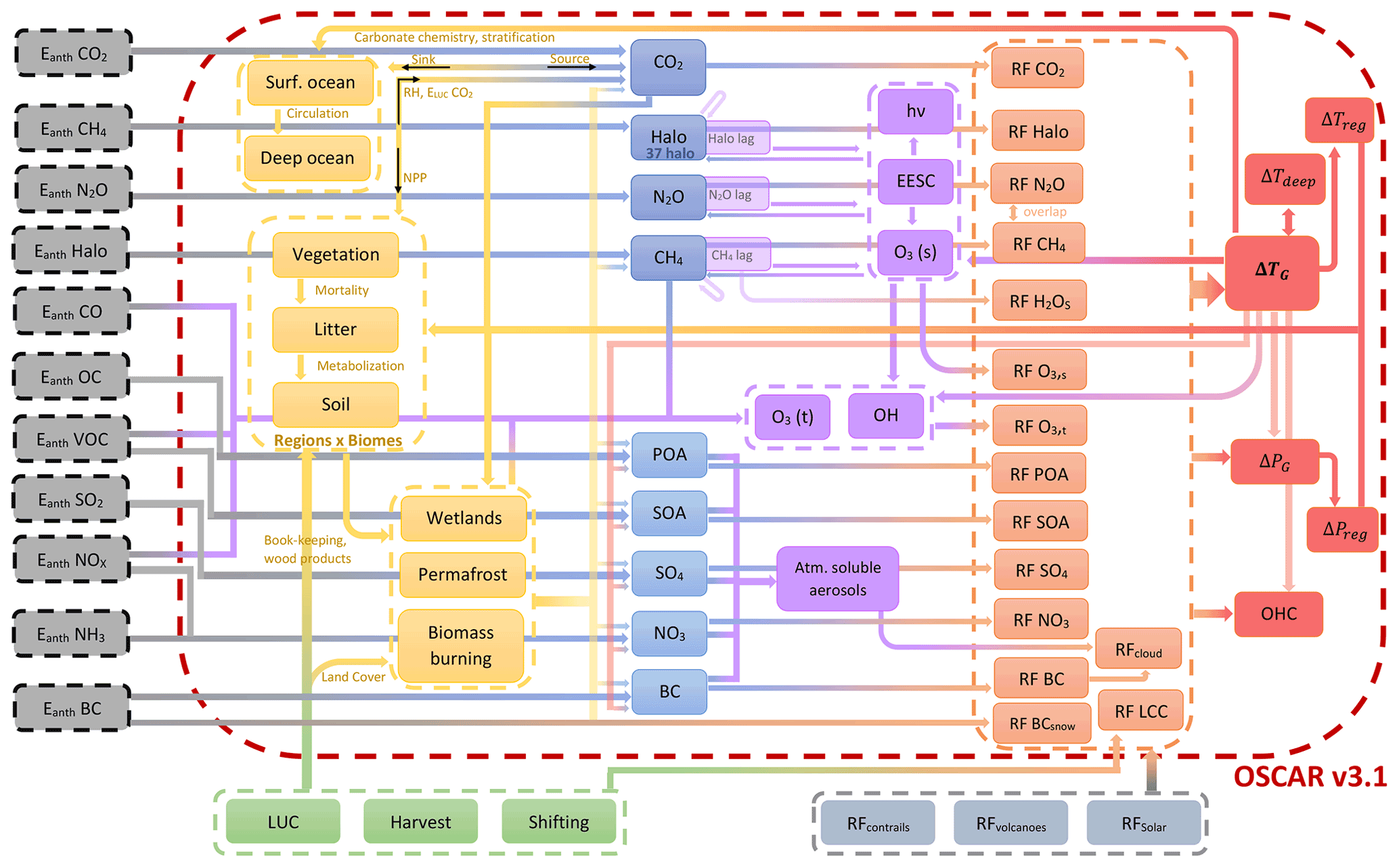
Figure 1 Conceptual figure of OSCAR v3.1. The central box with dashed red lines illustrates the framework of OSCAR v3.1, taking as inputs anthropogenic emissions (dark-grey boxes), land-use and land-cover change (green boxes), and additional radiative forcings (light-grey boxes). The components of OSCAR v3.1 are organized in this figure by category: ocean carbon, land carbon and other land processes are in yellow boxes, while atmospheric concentrations are in blue boxes, atmospheric chemistry in purple boxes, radiative forcings in orange boxes and climate system in red boxes. The complete description of OSCAR v2.2 is in Gasser et al. (2017), while the update to OSCAR v3.1 is described in Gasser et al. (2020).

2 Experimental setup

2.1 Brief description of OSCAR v3.1

OSCAR v3.1 is an open-source Earth system model of reduced complexity, whose modules mimic models of higher complexity. OSCAR is meant to be used in a probabilistic fashion (Gasser et al., 2017). A conceptual description of OSCAR v3.1 is given in Fig. 1. The full description of OSCAR v2.2 can be found in Gasser et al. (2017), providing details on its structure, equations and calibration. Changes from v2.2 to v3.1 are detailed in Gasser et al. (2020).

Global surface temperature changes in response to radiative forcing follows a two-box model formulation (Geoffroy et al., 2013b). Global precipitation is deduced from global surface temperature and the atmospheric fraction of radiative forcing (Shine et al., 2015). Linear scaling on the global variables is used to estimate regional temperature and precipitation changes, over five broad world regions (IIASA, 2018b). OSCAR calculates the radiative forcing caused by greenhouse gases (CO₂, CH₄, N₂O and 37 halogenated compounds), short-lived climate forcers (tropospheric and stratospheric ozone, stratospheric water vapor, nitrates, sulfates, black carbon, and primary and secondary organic aerosols) and changes in surface albedo.

The ocean carbon cycle is based on the mixed-layer response function of Joos et al. (1996), albeit with an added stratification of the upper ocean derived from CMIP5 (Arora et al., 2013) and with an updated carbonate chemistry. The land carbon cycle is divided into five biomes and the same five regions as previously. Each of the 25 biome–region combinations follows a three-box model (soil, litter and vegetation) described by Gasser et al. (2020). The preindustrial state of the land carbon cycle is calibrated against TRENDYv7 (Le Quéré et al., 2018a), and its transient response to CO₂ and climate is calibrated against CMIP5 models (Arora et al., 2013).

OSCAR endogenously estimates key aspects of the carbon cycle. A dedicated book-keeping module tracks land-cover change, wood harvest and shifting cultivation, which allows OSCAR to estimate its own CO₂ emissions from land-use change (Gasser et al., 2020; Gasser and Ciais, 2013). Permafrost thaw and the resulting emissions of CO₂ and CH₄ are also accounted for in Gasser et al. (2018). CH₄ emissions from wetlands are calibrated on WETCHIMP (Melton et al., 2013). In addition, biomass burning emissions are calculated endogenously on the basis of the book-keeping module and wildfires that are simulated as part of the land carbon cycle (Gasser et al., 2017). The latter emissions were subtracted from the input data used to drive OSCAR to avoid double counting.

The atmospheric lifetimes of non-CO₂ greenhouse gases are impacted by non-linear tropospheric (Holmes et al., 2013) and stratospheric (Prather et al., 2015) chemistries. Tropospheric ozone follows the formulation by Ehhalt et al. (2001) but recalibrated on ACCMIP (Stevenson et al., 2013). Stratospheric ozone is derived from Newman et al. (2007) and Ravishankara et al. (2009). Aerosol–radiation interactions are based on CMIP5 and AeroCom2 (Myhre et al., 2013), while aerosol–cloud interactions depend on the hydrophilic fraction of each aerosol and follow a logarithmic formulation (Hansen et al., 2005; Stevens, 2015). Surface albedo change induced by land-cover change follows (Bright and Kvalevåg, 2013). The impact of black carbon deposition on snow albedo is calibrated on ACCMIP globally (Lee et al., 2013) and regionalized following Reddy and Boucher (2007).

We pinpoint that OSCAR v3.1 is still calibrated on CMIP5 ESMs and therefore not meant to emulate CMIP6 models. Furthermore, each module is calibrated on available models, but not all ESMs have implemented every aspect modeled in OSCAR, such as permafrost or biomass burning. It means that OSCAR does not emulate any given ESM, but it combines modules emulating specific parts of these models. Every parametrization of OSCAR is thus a combination of parameters, and some of these combinations may be unrealistic and need post-processing to keep only the physically realistic ones, as explained in Sect. 2.3.

Table 1 List of CMIP6 and RCMIP simulations run with OSCAR. Standard names are used, and a full description of the experiments is provided in references. Every experiment that is a scenario has been run with its extension up to 2500. A spin-up of 1000 years is associated with each of the eight control experiments.

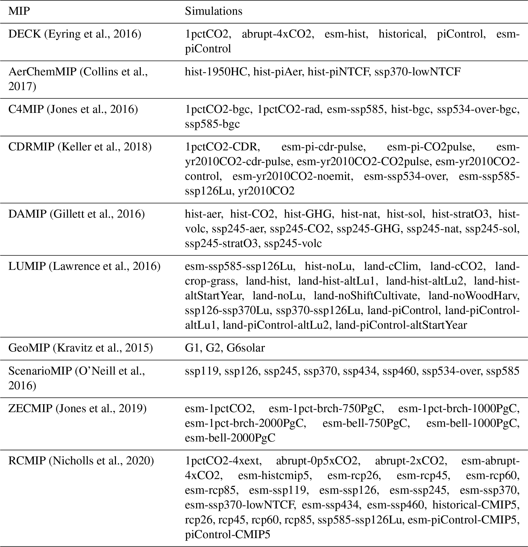
2.2 CMIP6 and RCMIP experiments

A total of 99 experiments were run with OSCAR, 75 being from CMIP6 and 24 from RCMIP. A list of these experiments is provided in Table 1. We selected the experiments according to several criteria: typically, experiments are global and/or with long time series of output requested, and experiments do not overly focus on a given process or short timescales. In addition, RCMIP requested additional experiments to complement those of CMIP6, mostly extended and additional scenarios, including the Representative Concentration Pathway (RCP) scenarios from the previous CMIP5 exercise (Meinshausen et al., 2011b). Between the CMIP5 and CMIP6 historical simulations, the concentration- and emission-driven ones, and the land-only experiments of LUMIP, eight different spin-up and control experiments had to be performed. Every spin-up is a recycling of the preindustrial forcing over 1000 years.

We use driving data sets for historical concentrations of greenhouse gases (Meinshausen et al., 2017), projected concentrations of greenhouse gases (ESGF, 2018), emissions (IIASA, 2018a; Gidden et al., 2019; Hoesly et al., 2018), land use (LUH2, 2018), solar activity (Matthes et al., 2017), volcanic activity (Zanchettin et al., 2016) and the land-only climate climatology for LUMIP experiments (Lawrence et al., 2016). The extensions of scenarios are not those that were initially foreseen (O'Neill et al., 2016) but those that have effectively been used during the CMIP6 exercise (Meinshausen et al., 2020). The volcanic aerosol optical depth has been treated to scale and extend AR5 volcanic radiative forcing (IPCC, 2013) to comply with the requirement of OSCAR to have a radiative forcing as driver for this contribution.

Every single experiment is run for 10 000 different configurations of OSCAR, drawn randomly from the pool of all possible parameter values in a Monte Carlo setup (Gasser et al., 2017). Altogether, the combined experiments and Monte Carlo members sum to 569 700 000 simulated years.

2.3 Post-processing: exclusion and constraining

As described in Gasser et al. (2017), most of the equations of OSCAR may use different sets of parameters or even different forms of equations. These parameters arise from the training over different models, while the forms of equations find their justification in the literature. Each combination of parameters and equations is defined as a configuration of OSCAR and represents a different possible model of the Earth system. A Monte Carlo setup is used with OSCAR over these configurations. This method for the uncertainty in the modeling of the Earth system comes with two side-effects: some combinations may be physically unrealistic, and some parameterizations may become numerically unstable when the model is pushed to the edge of the validity domain of its parametrizations. Therefore, the raw outputs of the simulations undergo two rounds of post-processing: one to exclude the diverging simulations and one to constrain the resulting Monte Carlo ensemble. We remind that the same exclusions and constraints are used for the contribution of OSCAR in RCMIP phase 2 (Nicholls et al., 2021b). All details about the method are provided in Appendix A. All final outputs and results are provided as the resulting weighted means and standard deviations, using the normalized likelihood as weight. The effect of this constraining is further discussed in the next section.

3 Evaluation of OSCAR v3.1

In the previous section, we give an overview of OSCAR, explain which experiments are run and shortly describe how the results are processed. Given this experimental setup, we evaluate how OSCAR reproduces key features by comparing against other models and observations. We investigate the extent of the corrections brought by the constraints in Sect. 3.1. As the two main components of the Earth system, the climate and carbon cycle responses are then respectively investigated in Sect. 3.2 and 3.3. We evaluate the capacity of OSCAR to reconstruct the historical period in Sect. 3.4 and calculate the contributions of individual forcings over the historical warming in Sect. 3.5. After evaluating the historical period, we evaluate how OSCAR performs on scenarios, comparing against ESMs in Sect. 3.6. The zero-emissions commitment is presented in Sect. 3.7 to compare the performance of OSCAR with respect to other models. Additional experiments are used to provide insights on the behavior of OSCAR, albeit not used for evaluation of the model, as detailed in Sect. 3.8 and Appendix B.

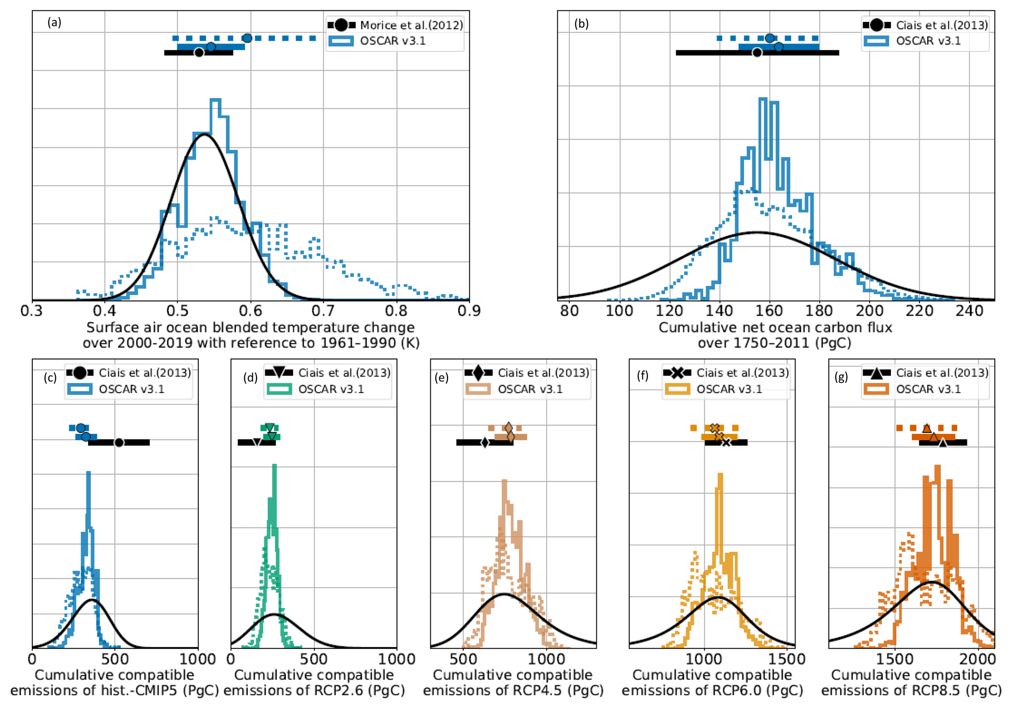
Figure 2 Effect of the constraining step. The histograms are the results of OSCAR v3.1, with plain lines being for the constrained version, while the dotted lines are for the unconstrained version. Horizontal lines correspond to the average ±1 standard deviation. Cumulative compatible carbon emissions in PgC from historical-CMIP5 are calculated over 1850–2011, while those of the RCPs are calculated over 2012–2100.

3.1 Effect of the constraints

Our constraining approach corrects natural biases in OSCAR, as illustrated in Fig. 2. The change in global surface air temperature (GSAT) over 2000–2019 with regard to 1961–1990 is constrained to a value of 0.54±0.05 K. Without the constraint, OSCAR v3.1 reaches 0.60±0.11 K. Due to the combination of observational constraints, OSCAR v3.1 is corrected to 0.55±0.04 K.

Regarding the carbon cycle, the unconstrained OSCAR shows a negative bias in the cumulative net land carbon sink (i.e. a too weak removal), balanced by lower cumulative compatible fossil-fuel emissions. Observational constraints reduce these biases but do not entirely remove them. After applying the constraints, the uncertainty ranges of the net land flux and of fossil-fuel emissions are reduced. Similarly, the ocean carbon sink over 1750–2011 of the unconstrained OSCAR is 159±20 PgC, higher than the one of IPCC AR5 (Ciais et al., 2013b), 155±18 PgC, in terms of mean and standard deviation. The constraints on cumulative compatible emissions mostly impact RCP6.0 and RCP8.5, transforming the bimodal distribution of the unconstrained OSCAR into a monomodal distribution. Using this constraint, the mean of OSCAR is increased and the range decreased, reaching 163±15 PgC.

Applying these constraints successfully reproduces the observed distribution but also reduces the range in the other constraints, such as the cumulative net ocean carbon flux over 1750–2011. We note that combining these constraints leads to a tightening of the posterior distribution, thus likely introducing a bias. OSCAR could benefit from further development in this direction, following McNeall et al. (2016) and Williamson and Sansom (2019).

3.2 Climate response

Simulations with an abrupt increase in atmospheric CO₂ (and thus in radiative forcing) are typically used to evaluate the climate response of complex models. We use three such experiments from CMIP6 and RCMIP with quadrupled, doubling and halving atmospheric CO₂ (abrupt-4xCO2, abrupt-2xCO2 and abrupt-0p5xCO2). These experiments can be used to estimate the equilibrium climate sensitivity (ECS) of an ESM or a model such as OSCAR (Gregory et al., 2004) and investigate how this metric is influenced by the intensity of the forcing. The results are shown in Fig. 3.

The ECS is defined as the equilibrium temperature that results from the doubling of the preindustrial atmospheric concentration of CO₂ (Gregory et al., 2004). The ECS and its calculations have evolved with the integration of new components into climate models (Meehl et al., 2020). In regard of the computational cost of the ESMs, reaching this equilibrium takes a time long enough to use Gregory's method (Gregory et al., 2004) to calculate the ECS or alternative methods (Lurton et al., 2020; Schlund et al., 2020). The ECS using the Gregory method is actually not exactly the equilibrium climate sensitivity per se but rather an “effective climate sensitivity” (Sherwood et al., 2020). Paleoclimate data show that feedbacks from vegetation, biogeochemistry or dust affect the equilibrium (Friedrich et al., 2016; Rohling et al., 2012). From CMIP5 to CMIP6, ESMs have improved their treatment of the biogeochemistry and the vegetation, leading to alteration in feedbacks and aerosol fields (Meehl et al., 2020). This evolution participates in the observed changes in ECS from CMIP5 to CMIP6, attributed to cloud effects (Zelinka et al., 2020) and the pattern effect (Dong et al., 2020).

In OSCAR, there are two ways of estimating the ECS. First, because OSCAR is not process-based, the ECS is actually a parameter of the model. Since the formulation of the climate module is linear (Gasser et al., 2017; Geoffroy et al., 2013b), we also know that this value is independent of the intensity of the abrupt experiment. This parameter was calibrated on the abrupt-4xCO2 experiment run by CMIP5 models and normalized to OSCAR's estimate of radiative forcing (RF) for a quadrupling of CO₂ (Gasser et al., 2017). Under this definition, the ECS of OSCAR follows Gregory's method and does not account for all feedbacks of OSCAR. When using parameters from OSCAR, the climate feedbacks included in the estimated ECS depend on the CMIP5 models used for calibration. If calibrated on general circulation models (GCMs), only the so-called Charney feedbacks are included (i.e. Planck, water vapor, lapse rate, sea-ice albedo and clouds), with the possible addition of the CO₂ physiological feedback (Sellers et al., 1996). However, when calibrated on ESMs, additional feedbacks relative to interactive biogeochemical cycles may be included, depending on what exact processes are implemented in a given ESM. The second way of estimating the ECS in OSCAR is to define it as the GSAT change at the end of the 1000 years of the abrupt experiments. Here, all of the feedbacks integrated in OSCAR are accounted for, especially biogeochemical feedbacks.

Table 2 Metrics of the climate system (ECS, TCR and TCRE). Metrics are provided for OSCAR v3.1, constrained using observations and unconstrained. Values are provided as mean ± standard deviation, median and the [5 %–95 %] confidence interval. As explained in Sect. 3.2, the ECS in OSCAR may be calculated using its parameters, or simply as the temperature at the end of abrupt-2xCO2. These values are compared to the ECS of Meehl et al. (2020). The same source provides the values for the TCR. The TCRE of CMIP5 is compared to Gillett et al. (2013). Values from RCMIP phase 2 (Nicholls et al., 2021b) come from different sources: Sherwood et al. (2020) for the ECS, Tokarska et al. (2020) for the TCR and Arora et al. (2020) for the TCRE.

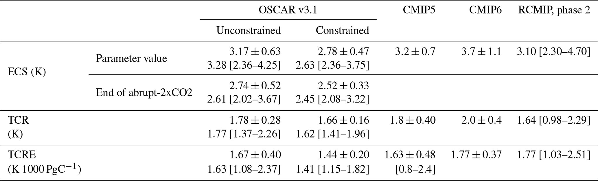
Values related to these two approaches are presented in Table 2. The ECS calculated using parameters of OSCAR, hence comparable to Gregory's approach, is 2.78±0.47 K when constrained, while the unconstrained one is 3.17±0.63 K. By construction, this is consistent with the AR5 estimates (Collins et al., 2013) but also with more recent assessments (Gregory et al., 2020). Because we use observational constraints, these results are lower than the CMIP5 range 2.1–4.7 K (Andrews et al., 2012). The CMIP6 range, 1.8–5.6 K (Zelinka et al., 2020; Meehl et al., 2020), is even higher than the CMIP5 range. The higher values for the ECS from some CMIP6 models are significantly reduced when constraining (Nijsse et al., 2020; Bonnet et al., 2021), with some ECS estimates even lower than those shown here, such as 1.38 K, with a likely range of 1.3–2.1 K. Overall, these values provided by OSCAR remain consistent with the literature, albeit at the lower end of the range (Sherwood et al., 2020). As shown in Table 2, the transient climate response (TCR) and the transient climate response to emissions (TCRE) of the unconstrained OSCAR are also consistent with the CMIP5 values in Meehl et al. (2020) and Gillett et al. (2013), thanks to the calibration of the ECS in OSCAR. Constraining OSCAR reduces all these metrics, both in value and in range. We attribute this effect to the constraint on historical warming. This reduction effect is similar to what was shown recently for CMIP6 models (Tokarska et al., 2020).

Figure 3 Abrupt idealized experiments. In (a) the plain lines represent the average change in surface air temperature, and its ±1 standard deviation ranges using shaded areas. Panels (b, c, d) show the contributions to the total RF at equilibrium. Individual contributions from stratospheric O₃ and deposition of black carbon (BC) on snow are inferior to 0.1 W m⁻² in the abrupt-4xCO2 and have not been represented for clarity. Panels (e, f, g) are the distributions of the ECS, calculated using equilibrium temperature, and thus include all the feedbacks of OSCAR. The horizontal plain line is the ECS average and ±1 standard deviation range. These values with Pearson's moment coefficient of skewness are provided in the legend.

The other approach to derive ECS using abrupt experiments is illustrated in Fig. 3. It leads in abrupt-2xCO2 to an unconstrained ECS of 2.74±0.52 K (Table 2), reduced to 2.52±0.33 K with the constraints. Overall, the ECS is remarkably consistent in terms of average, standard deviation and even skewness across the three abrupt experiments. This is due to the construction of OSCAR, with a prescribed logarithmic dependency of the radiative forcing of CO₂ on its atmospheric concentration (Lurton et al., 2020). This ECS is lower than with the first approach because it includes several Earth system feedbacks related to short-lived species that are left free to change during the simulations, owing to the experimental protocol. In OSCAR, this is mostly explained by an increase in the atmospheric load of tropospheric aerosols (and ozone) caused by the endogenous emission of precursors through biomass burning. These feedbacks are also illustrated in Fig. 3. The RF resulting from the prescribed change in atmospheric CO₂ (7.42 W m⁻² under quadrupled CO₂) is partially compensated for by short-lived climate forcers. In the case of abrupt-4xCO2, the RF sums up to 3.46±0.25 W m⁻² because of a cooling by scattering aerosols ($-\mathrm{0.21}\pm \mathrm{0.16}$ W m⁻²) and aerosol–cloud effects ($-\mathrm{0.21}\pm \mathrm{0.15}$ W m⁻²), besides an additional warming from absorbing aerosols (0.13±0.08 W m⁻²). Finally, from Table 2, we note that constraining reduces the parameter-based ECS by 0.44 K, while the one with all feedbacks has its ECS reduced by 0.22 K, which implies that biogeochemical feedbacks are also significantly constrained.

Figure 4 Experiments with 1 % increase in the atmospheric CO₂. The plain lines are the averages, and the shaded areas represent ±1 standard deviation ranges.

3.3 Carbon cycle response

The 1pctCO2 experiment, in which atmospheric CO₂ increases by +1 % every year, is part of the DECK. Two variants of 1pctCO2 have been performed as part of the C4MIP exercise (Fig. 4). In 1pctCO2-rad, atmospheric CO₂ only has a radiative effect on the climate system, as a preindustrial level of CO₂ is seen by the carbon cycle. In 1pctCO2-bgc, only the carbon cycle is affected by CO₂, whereas a preindustrial CO₂ is prescribed to the climate system. The outputs of OSCAR v3.1 on these experiments are consistent with past C4MIP results (Arora et al., 2013). The global mean surface temperature responds about linearly to the exponential increase in CO₂ because of the implemented logarithmic dependency of the radiative forcing of CO₂ on its atmospheric concentration. Carbon sinks rise in response to the increase in atmospheric CO₂, but the resulting warming dampens the sinks.

Table 3 Metrics of the carbon cycle (β and γ) from the C4MIP experiments. Metrics are provided for OSCAR v3.1, constrained using observations and unconstrained. As explained by Arora et al. (2013), different values for the metrics are calculated depending on the combination of experiments used: R stands for radiative (1pctCO2-rad), B for biogeochemical (1pctCO2-bgc) and F for full (1pctCO2). The change in the land carbon stocks includes permafrost carbon. Results from CMIP5 and CMIP6 are provided by C4MIP (Arora et al., 2020).

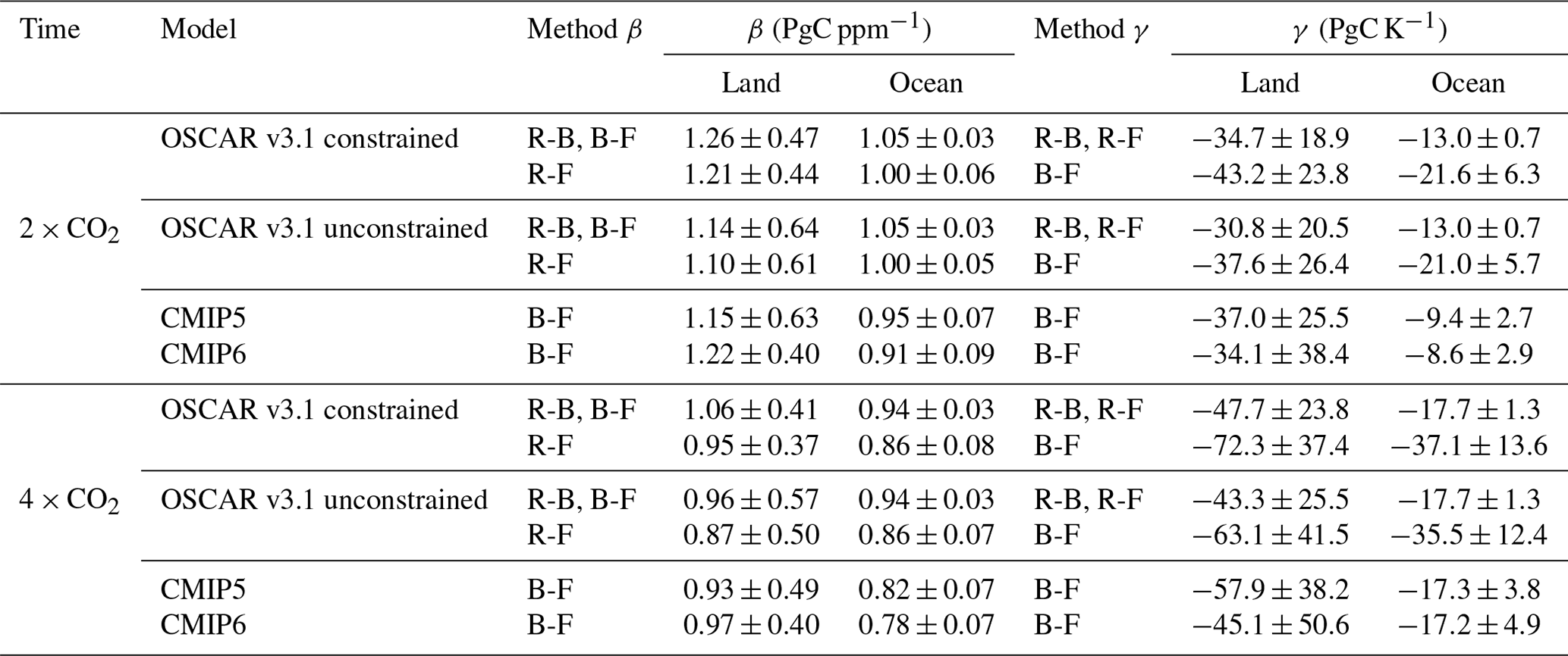
These three experiments can be used to calculate the carbon-concentration and carbon-climate feedback metrics, respectively β and γ. These metrics, defined and used in former C4MIP exercises (Friedlingstein et al., 2006; Arora et al., 2013, 2020), are a means to evaluate the model's sensitivities of the carbon stocks in the land and in the ocean to changes in atmospheric CO₂ or GSAT. Table 3 summarizes these results. As explained by Arora et al. (2013), there are three methods to combine the three experiments to calculate the metrics: subtracting 1pctCO2-bgc from 1pctCO2-rad (denoted R-B, hereafter), subtracting 1pctCO2 from 1pctCO2-bgc (B-F) and subtracting 1pctCO2 from 1pctCO2-rad (R-F). As shown in Table 3, methods R-B and B-F are almost equivalent for β, while methods R-B and R-F are almost equivalent for γ. Although LUC affects these metrics (Melnikova et al., 2022), these experiments are designed to have a constant LUC.

Table 3 shows that β under the R-F method is lower than the R-B and B-F because the non-linearity of the Earth system reduces the sensitivity of land and ocean carbon to atmospheric CO₂. Similarly, γ under the R-B and R-F is higher than under the B-F, but the non-linearity here is added to R-B and B-F (Arora et al., 2013). Applying our observational constraints increases the absolute values of β_land and γ_land of OSCAR, but it does not affect the β_ocean and γ_ocean significantly. The only exception is the γ_ocean under the method B-F. We note that the unconstrained OSCAR v3.1 is closer to the CMIP5 exercises, be it at 2× or 4× CO₂. This result can be explained with OSCAR v3.1 being calibrated on CMIP5. However, the unconstrained β_land is the only one to be closer to CMIP6 than to CMIP5. The cause of this difference in the β_land remains unclear but may come from the form of equation for the fertilization effect. The configurations of OSCAR are not only different parameters, but also different equations. Here, half of the configurations of OSCAR follow a logarithmic formulation of the fertilization effect (Gasser et al., 2017), which may not be convex enough to properly represent a saturation effect found in many ESMs. We note that in our assessment, the land includes permafrost carbon, which was not the case in CMIP5 assessment, but the permafrost is mostly sensitive to increase in temperatures (i.e. it impacts γ_land but not β_land).

Overall, Table 3 shows that the unconstrained carbon cycle of OSCAR v3.1 is in line with CMIP exercises, particularly CMIP5. Yet, the sensitivity of the oceanic carbon stock to increase in GSAT remains too high. This bias in the ocean module could be attributed to the stratification effect introduced in v2.2 (Gasser et al., 2017). In any case, this suggests that our carbon cycle may be too optimistic, which will clearly appear in our emission-driven simulations.

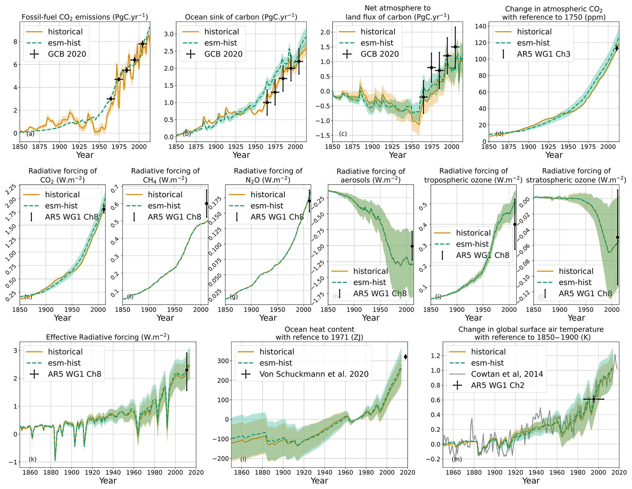
Figure 5 Emission- and concentration-driven historical scenarios. The plain lines are the averages, and the shaded areas represent ±1 standard deviation ranges. The fossil-fuel CO₂ emissions for the concentration-driven historical simulation are the compatible emissions, whereas those for the emissions-driven esm-hist are directly prescribed to OSCAR. Radiative forcings under esm-hist are not represented, for they are too close to the concentration-driven historical simulation. Radiative forcings are with respect to 1750. The sources for the observations are Friedlingstein et al. (2020) for GCB 2020, Hartmann et al. (2013) for AR5 WG1 Ch2, Ciais et al. (2013b) for AR5 WG1 Ch3 and Myhre et al. (2013) for AR5 WG1 Ch8. The 90 % ranges provided by AR5 are converted to the ±1 standard deviation ranges.

3.4 Reconstruction of the historical period

The concentration- and emission-driven historical experiments (i.e. historical and esm-hist simulations, respectively) were run with OSCAR. Their forcers differ only for CO₂: the atmospheric CO₂ is prescribed in the former, whereas in the latter, fossil-fuel emissions are prescribed, and atmospheric CO₂ is fully interactive. In the concentration-driven historical simulation, compatible fossil-fuel emissions are back-calculated after the simulation (Jones et al., 2013; Gasser et al., 2015). Altogether, these two simulations are relatively close, as shown in Fig. 5, but with noticeable differences.

Looking at the carbon cycle variables, we observe that up to the 1940s, esm-histis was similar to the historical simulation in terms of fossil-fuel CO₂ emissions, atmospheric CO₂ and both carbon sinks. For instance, the cumulative ocean sink over 1850–1940 is respectively 41 and 35 PgC in historical and esm-hist simulations. The difference observed afterwards can essentially be explained by the fact that the emission-driven simulation entirely misses the 1940s plateau in atmospheric CO₂. Such a miss is typical of ESMs (Bastos et al., 2016). For comparison after 1959, we use data from the Global Carbon Budget (Friedlingstein et al., 2020), whose assessment of ocean carbon sink is closer to our historical simulation than to our esm-hist simulation. The net carbon flux from atmosphere to land (i.e. the aggregate of the land sink, emissions from LUC and emissions from permafrost) of the two historical experiments is similar from the 1980s onward. For comparison, the estimate for this average net land flux is 1.5±1.1 PgC yr⁻¹ over 2000–2009 (Friedlingstein et al., 2020), while this flux calculated by OSCAR under historical and esm-hist simulations is 0.88±0.48 and 0.85±0.56 PgC yr⁻¹, respectively.

Looking at the effective radiative forcings (ERFs), the ERF of CO₂ in the concentration-driven historical simulation is directly deduced from the prescribed CO₂ atmospheric concentration (Meinshausen et al., 2017) but slightly higher by about 0.1 W m⁻² than the central value from the 5th Assessment Report (AR5) (Myhre et al., 2013). The central value from AR5 (1.82 W m⁻²) is calculated with reference to 1750 but becomes 1.66 W m⁻² when calculated with reference to 1850. This value increases to 1.70 W m⁻² in CMIP6 data, mostly because of changes in the CO₂ concentration in 1850. With OSCAR and prescribed CO₂ emissions, the atmospheric CO₂ in esm-hist is higher than in the historical simulation, and the ERF of CO₂ is 0.2 W m⁻² higher than in the AR5. The ERF of other greenhouse gases is consistent with Myhre et al. (2013). For most ERF components, there is very little difference between historical and esm-hist. OSCAR's overall ability to simulate the RF of short-lived species compares well with the IPCC AR5 values. Contributions to the warming from aerosols and ozone are consistent as well, although OSCAR tends to amplify these contributions. In 2011, IPCC AR5 estimates the RF from aerosols to be $-\mathrm{1.01}\pm \mathrm{0.37}$ W m⁻², while OSCAR calculates this to be $-\mathrm{1.29}\pm \mathrm{0.52}$ W m⁻². Similarly, IPCC AR5 estimates the RF from tropospheric ozone in 2011 to be 0.4±0.2 W m⁻², and OSCAR estimates the RF to be 0.50±0.05 W m⁻². It may be caused by overestimated biomass burning emissions, and this will be examined more in depth in a future analysis. Since these biases were already evaluated in the description paper of OSCAR (Gasser et al., 2017), it shows that our constraining does not markedly alter these aspects of the model. Additional constraining could be introduced for separate RF components, although this would likely weaken the efficiency of other existing constraints.

Looking at climate variables, the increase in GSAT in both historical experiments is consistent with the Special Report on Global Warming of 1.5C (IPCC, 2018) and with the historical reconstruction by Cowtan and Way (2013). During the choice of constraints (Sects. 2.3 and 3.1, Appendix A), we observed that constraints on temperatures impact our results much more than the other type of constraints. Even while the set of constraints is expanded, constraints on temperature have a lasting influence over all outputs. The esm-hist simulation shows a higher GSAT and appears to be further away from the observations. This is mostly the result of the higher atmospheric CO₂ seen earlier, and it suggests a different set of constraining weights could be used for the emission-driven runs. We choose not to, for the sake of consistency. Comparing the effective radiative forcing (ERF) of OSCAR to the one of the IPCC AR5 (Myhre et al., 2013), we note differences caused by volcanic eruptions. Beyond the update of the time series of volcanic activity itself, OSCAR make use of a warming efficacy of 0.6 for stratospheric volcanic aerosols (Gasser et al., 2017; Gregory et al., 2016). Nevertheless, IPCC AR5 estimates the ERF to be 2.3±1.0 W m⁻², while OSCAR calculates the ERF under historical and esm-hist simulations to be 2.24±0.48 and 2.34±0.50 W m⁻², respectively. Finally, the total ocean heat content is well reconstructed, although the range of OSCAR is larger than the observed one (von Schuckmann et al., 2020), suggesting this could also be considered a potential constraint for the model in future work.

Table 4 Attribution of historical and future climate change. These contributions come either from experiments in which only the concerned forcing was prescribed (DAMIP) or from experiments in which it was removed (other MIPs). In either cases, non-linearities are ignored.

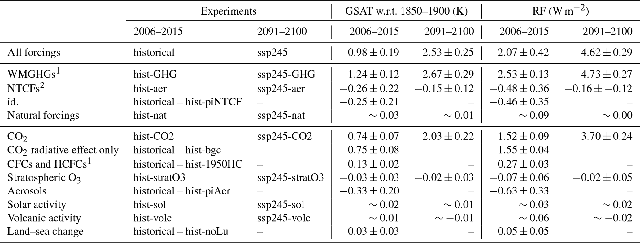
¹ In these experiments, because the atmospheric concentration of WMGHGs is prescribed, the indirect effects on tropospheric O₃ (from CH₄), stratospheric H₂O (from CH₄) and stratospheric O₃ (from N₂O and halogenated compounds) are also included. ² The effects listed in the previous note on WMGHGs are excluded from this experiment. Tropospheric O₃ does vary but only because of the emission of ozone precursors and not because of varying atmospheric CH₄. Black carbon deposition on snow is also included in this experiment.

3.5 Attributions

DAMIP (Gillett et al., 2016) designed a number of experiments meant to attribute the observed climate change to anthropogenic and natural factors. Since OSCAR does not feature any internal variability, it cannot contribute to the “detection” part of DAMIP. However, with more than 1000 Monte Carlo elements, OSCAR is fully capable of carrying out the “attribution” part. To achieve this attribution, DAMIP relies on experiments that follow the historical one but in which only one forcing is turned on. Conversely, a number of other MIPs introduced attribution experiments in which all forcings but the ones studied are turned on. However, neither of these approaches explicitly considers the non-linearities of the system. Other more robust methods of attribution to forcings exist (Trudinger and Enting, 2005) and have been used with OSCAR in the past (Gasser, 2014; Li et al., 2016; Fu et al., 2020; Ciais et al., 2013a). Here, we focus on results made possible with the CMIP6 experiments, which are presented in Table 4.

In the historical experiment, we find a change in GSAT of 0.98±0.17 K in 2006–2015 with regard to 1850–1900, which is in line with observations because of our constraining setup (Sect. 2.3). Natural forcings caused only ∼0.03 K of this total, of which ∼0.02 and ∼0.01 were respectively caused by solar and volcanic activity. Note that our volcano-related forcing is defined against an average and constant volcanic activity during the preindustrial period. This is why the volcanic activity contributes only a positive ∼0.01 K over the recent past where no major volcanic eruption happened. In the IPCC terminology, our results lead to the conclusion that it is extremely unlikely (i.e. likelihood <1 %) that natural factors alone are causing the current observed climate change. This is of course consistent with the IPCC conclusions (Eyring et al., 2021; Gillett et al., 2021). Nevertheless, we note that our constraining reduces the uncertainty range of all simulations, including those driven only by natural forcings. For the simulations under natural forcings, the range from the constrained OSCAR is smaller than the ones from Gillett et al. (2021), which may suggest an over-constraining. It may be solved using different methods for constraining climate simulations (Nicholls et al., 2021b; Williamson and Sansom, 2019).

Since DAMIP did not include an experiment in which only natural forcings would be turned off, we cannot conclude as to the complementary probability of observed climate change being caused only by anthropogenic factors (Gillett et al., 2021). Attribution to groups of anthropogenic forcings is possible, however. We find that 1.25±0.11 K, about 128 % of the recent warming, was caused by well-mixed greenhouse gases (WMGHGs), and $-\mathrm{0.26}\pm \mathrm{0.22}$ K (−27 %) was by near-term climate forcers (NTCFs). For comparison, the 90 % confidence interval of CMIP6 over 2010–2019 instead of 2006–2015 is 1.16 to 1.95 K for WMGHGs and −0.73 to −0.14 K for NTCFs (Gillett et al., 2021). Another contribution of $-\mathrm{0.03}\pm \mathrm{0.03}$ K (−3 %) is due to land-use change. We highlight that observational constraints affect these contributions, as shown by Ribes et al. (2021), whose central estimate contributions over 2010–2019 are 116 % for WMGHGs and −32 % for NTCFs and land-use change. It follows that the constrained results of OSCAR v3.1 are consistent with Gillett et al. (2021) and Ribes et al. (2021).

Considering the other experiments, we observe that the DAMIP experiment (hist-aer) and the AerChemMIP one (hist-piNTCF) led to very similar estimates of the contribution of NTCFs (Table 4), which highlights that this part of our model behaves in a linear fashion. Going further in isolating individual forcings, we also estimate that CO₂ caused 0.74±0.06 K, chlorofluorocarbons and hydro-chlorofluorocarbons (i.e., CFCs and HCFCs) caused 0.13±0.02 K, stratospheric O₃ caused $-\mathrm{0.03}\pm \mathrm{0.03}$ K and all aerosols together caused $-\mathrm{0.33}\pm \mathrm{0.21}$ K (including direct and indirect effects). We point out that details on CH₄, N₂O or tropospheric ozone cannot be provided because of the lack of relevant CMIP6 experiments.

The extent to which this attribution to specific forcings is comparable to existing studies remains unclear. One notable limitation of OSCAR, in this respect, is that the model's climate response is not forcing-dependent. The use of effective radiative forcing is supposed to ensure that the temperature response to CO₂ and non-CO₂ forcings is similar, at least for the long-term steady state (Myhre et al., 2013). However, recent work has pointed out that the response may strongly depend on the forcing agent (Marvel et al., 2016), thus casting a degree of doubt on our attribution results. More work to integrate such differentiated responses in reduced-complexity models is warranted.

Table 5 Projected atmospheric CO₂, RF and GSAT in SSPs. Concentration- and emission-driven experiments are shown and compared to available CMIP6 projections. Values in bold are assumptions or inputs. Experiments whose name start with esm- are emission-driven; others are concentration-driven. GSAT data from CMIP6 are provided as mean and standard deviation as well, with the number of models available in parentheses. Here, projections from OSCAR are constrained to observations, while CMIP6 results are raw, without any constraints (Tokarska et al., 2020).

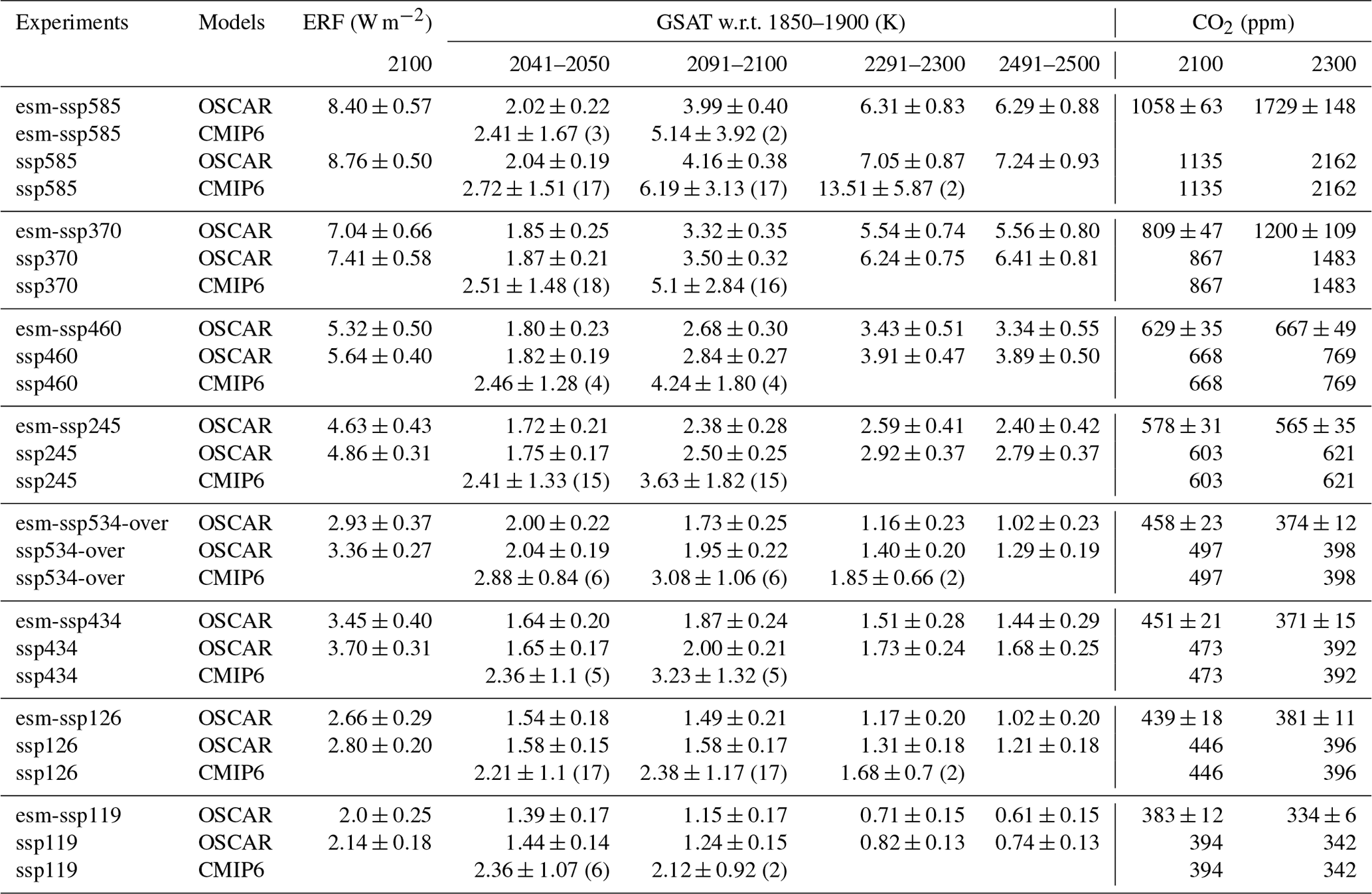
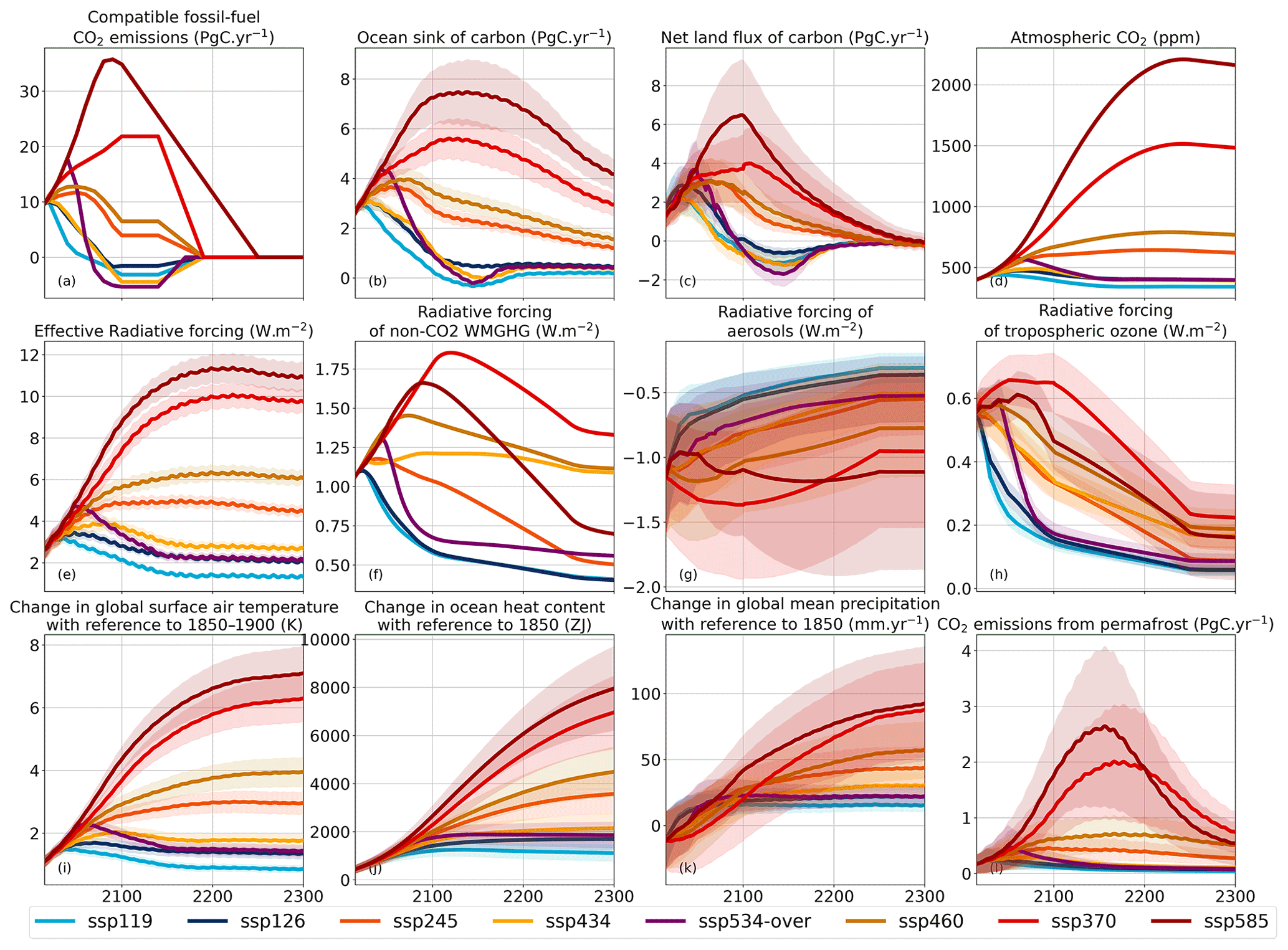
Figure 6 Global projections following the main CMIP6 scenarios in concentration-driven mode. Extensions are shown only up to 2300. The lines are the averages, and the shaded areas represent ±1 standard deviation ranges.

3.6 Scenarios of climate change

ScenarioMIP (O'Neill et al., 2016) chose eight particular Shared Socioeconomic Pathways (SSPs) taken from the SSP scenario database (Riahi et al., 2017) to cover a range of socio-economic assumptions and climate targets. After harmonization, these SSPs became the default CMIP6 scenarios to be run by ESMs (Gidden et al., 2019). ScenarioMIP mostly required concentration-driven simulations up to the year 2100 or 2300. In RCMIP, this was complemented by extending all scenarios up to 2500 and systematically running emission-driven simulations in addition (Nicholls et al., 2020). Figure 6 displays projections of key global variables of the Earth system following these scenarios, and Table 5 focuses on projected GSAT changes.

The climate target dimension of the SSP scenarios is defined similarly to the RCPs' as the total RF targeted in 2100 (van Vuuren et al., 2011). Table 5 shows that this targeted RF is overall within the 1σ uncertainty range of all our concentration-driven projections. In the cases with notable differences, such as ssp460, the actual RF reached by the reduced-complexity model MAGICC (IIASA, 2018a) for this scenario is 5.29 W m⁻², which is then in the range of OSCAR. Although MAGICC was used for the design of these scenarios, this result demonstrates that we remain consistent with the intended RF of the scenarios. Emission-driven SSPs show lower RF than their concentration-driven counterparts, which can be attributed to a low bias in the atmospheric CO₂ that is especially visible in high-CO₂ scenarios. This bias is a result of our constraining approach that favored configurations with strong CO₂ fertilization (as also seen with the C4MIP results, Sect. 3.3). Under high-CO₂ scenarios, this bias is likely worsened by our exclusion procedure during the post-processing, as very high CO₂ tends to make the model more unstable. The very low uncertainty range we obtain for projected atmospheric CO₂ in emission-driven simulations is over-confident. We note that the constraints were derived using concentration-driven simulations (that are the focus of CMIP6), and so they may not apply properly to emission-driven simulations.

The constraining approach contributes to having the increases in GSAT for concentration-driven experiments shown in Table 5 to be lower than the CMIP6 models we could compare our results to. The uncertainty range simulated by OSCAR is also much lower, again owing to our constraining approach. With a relative uncertainty in GSAT change in 2500 of ±13 % under the warmest scenario (SSP5-8.5), these projections are likely to be over-constrained. This stems from our constraining of the climate response, as also shown by the relatively small uncertainty range in ECS in the idealized abrupt CO₂ experiments. Further developing that module by adding one or two key parameters (Geoffroy et al., 2013a; Bloch-Johnson et al., 2015) would provide more degrees of freedom and likely release part of the constraint. When projecting temperature change in an emission-driven mode, the uncertainty range is larger because of the additional uncertainty related to the biogeochemical cycles.

The CMIP6 values are computed here from CMIP6 time series. However, some CMIP6 models exhibit higher warmings than in previous assessments, and observations can be used to constrain the future warming (Tokarska et al., 2020). Using their table S4, the warming in 2081–2100 with reference to 1995–2014 under SSP5-8.5 for the constrained CMIP6 models is 3.44±0.67 and 3.11±0.36 K for the constrained OSCAR v3.1 model. For SSP1-2.6, the values are respectively 0.94±0.30 and 0.76±0.17 K. Thus, the observational constraints that we have used contribute to explaining the differences to the raw CMIP6 data. Nevertheless, it remains that the climate module of OSCAR v3.1 could still be improved.

Figure 7 Change in global mean surface temperature for branched experiments (a, b) and bell experiments (c, d). The results over the zero-emission phase are shifted along the time axis so that t=0 corresponds to the time of cessation of emission. The lines are the averages, and the shaded areas represent ±1 standard deviation ranges.

3.7 Zero-emissions commitment

ZECMIP aims at investigating the zero-emission commitment (ZEC), that is the additional warming that follows a cessation of anthropogenic CO₂ emissions (Jones et al., 2019). Two categories of experiments were performed. The first one (called branched experiments) is a variation of the emission-driven 1pctCO2, in which emissions cease once they reach 750, 1000 or 2000 PgC of cumulative value. These distinct levels of cumulative emissions are meant to evaluate the state dependency of ZEC. The second category consists in three bell-shaped emission pathways, whose cumulative emissions are the same as in the branched experiments. This was proposed by ZECMIP to evaluate the dependency of the ZEC on CO₂ emission rate, as the emission rate at the time of cessation is near zero in these bell experiments, while it is very high in the branched ones.

Figure 7 shows the time series of the ZEC in both sets of experiments. In the branched experiments, the abrupt cessation of CO₂ emissions triggers an abrupt increase of temperature change, followed by a decrease. Conversely, since the cessation is smoother in the bell experiments, no abrupt response is visible on the very short term. After this period, the shape of the evolution of the ZEC in branched experiments is similar to the shape in bell experiments. We attribute this effect to the abrupt cessation of emissions in the branched experiments, causing biomass burning and aerosol lifetime feedbacks, whose response to temperature change happens within the same year. These feedbacks explain why the ZEC in branched experiments is systematically lower than the ZEC in bell experiments.

Table 6 Zero-emissions commitments at 25, 50, 90 and 500 years after emission cease. Only the ZECs for the esm-1pct-brch-1000PgC experiment are shown here, for comparison to results of ZECMIP. The full evolution of this experiment is shown in Fig. 7.

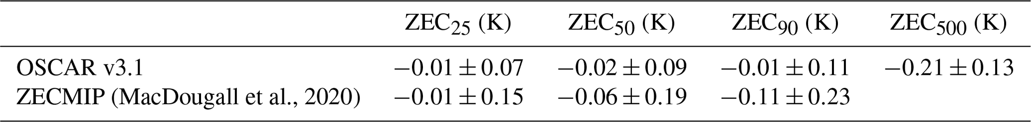
Figure 7 also shows that the ZEC for a cumulative emission of 2000 PgC is much higher than in the two other cases, highlighting a strong non-linearity in the model. We attribute this process to the permafrost response, in agreement with our previous work (Gasser et al., 2018). Once the branching year has been reached, anthropogenic emissions become zero, while natural systems such as the permafrost keep emitting. Among the models that contributed to ZECMIP (MacDougall et al., 2020), CESM2, NorESM2-LM and UVic ESCM 2.10 were the only ones to model permafrost, with only the latter one that provided data over the three branched experiments. As shown in Fig. 6 of MacDougall et al. (2020), UVic ESCM 2.10 is the model with the strongest evolution of the ZEC with cumulative emissions. This similar effect of permafrost on ZEC in OSCAR v3.1 and UVic ESCM 2.10 calls for more contributions of models with permafrost to the ZECMIP exercise and future similar projects.

As illustrated in Table 6, OSCAR v3.1 estimates a ZEC (in the reference case of the esm-1pct-brch-1000PgC experiment) that is within the range of ZECMIP (MacDougall et al., 2020). The evolution of OSCAR in this experiment is comparable to that of the Earth system models of intermediate complexity that contributed to the original ZECMIP.

3.8 Behavior of OSCARv3.1

The focus of this paper is to evaluate this version of OSCAR introduced in Gasser et al. (2020), and used with the same exclusion and constraining approach used for RCMIP phase 2 (Nicholls et al., 2021b). As explained in Sect. 2.2, many experiments have been run through OSCAR v3.1, and Sect. 3.1 to 3.7 have used only the experiments that would allow for clear comparison with ESMs and therefore evaluation. In the Appendix B, additional results are shown, further illustrating the behavior of OSCAR v3.1 under experiments that examine carbon geoengineering (Sect. B.1), solar geoengineering (Sect. B.2), land use (Sect. B.3), NTCFs (Sect. B.4) and a comparison of RCPs against SSPs (Sect. B.5). These additional experiments were not fully considered in the evaluation part of this study, typically because of the lack of published papers doing the same with fully fledged ESMs or because of non-existent evaluation metrics. These simulations can nevertheless provide valuable insights into the behavior of OSCAR, potentially helping understand past or even future contributions to community exercises such as CDRMIP or RCMIP.

4 Concluding remarks

In this study, we present the setup used with OSCAR v3.1 to run 75 CMIP6 and 24 additional experiments from RCMIP. We use the primary results of these simulations to discuss the overall behavior and performance of our model, comparing our results to those of state-of-the-art complex models whenever possible. We present a brief summary below of the model's main limitations.

First, the model tends to be unstable under high-CO₂ and high-warming scenarios. This comes mostly from the ocean carbon cycle module, whose stability is not ensured under our chosen differential system solving scheme, which is also worsened by the stratification feedback that was introduced in v2.2 (Gasser et al., 2017). This pleads for a revamp of this module.

Second, despite a clear improvement of the land carbon cycle module in v3.1 (Gasser et al., 2020), its unconstrained transient response remains wider than the ranges from CMIP5 or CMIP6 models, which makes the constraining step a strong requirement of any simulation with OSCAR. In its current state, the constraining step appears to favor parameterizations with a strong CO₂ fertilization effect. The extent to which this is caused by structural modeling choices is unclear. Consequently, the land carbon cycle also exhibits a sensitivity to climate change that is too low compared to complex models, mostly those without permafrost, thus calling for an improved calibration.

Third, the constrained climate module shows a relatively low ECS and a rather narrow uncertainty range. Introducing extra parameters for the heat uptake feedback (Geoffroy et al., 2013a) and possibly non-linear Charney feedbacks (Bloch-Johnson et al., 2015) would likely help to gain flexibility during the constraining. This third point is the reason behind most of the differences between OSCAR and CMIP6 temperature projections shown in Table 5.

Fourth, although most of the non-CO₂ species are reasonably simulated, the effects of tropospheric ozone and total aerosols tend to be overestimated. The whole aerosol module behaves rather linearly, and it exhibits a climate feedback whose intensity should be better constrained against existing simulations with complex ESMs. OSCAR would indeed benefit from further work on short-lived species, although this could prove a challenging endeavor given the aggregated formulation of the model and the uncertainties.

Finally, we have illustrated how observational constraints can be used to inform projections and how they may affect the results, such as the strong decrease of uncertainties in projections. Given the growing importance of these constraints (Tokarska et al., 2020; Nicholls et al., 2021b), this calls for investigating computationally efficient and physically sensible ways of doing so with OSCAR. Investigating and controlling the bias introduced in these steps may increase the confidence in the model's results (McNeall et al., 2016; Williamson and Sansom, 2019).

In spite of these limitations, we have demonstrated that OSCAR behaves as one would expect from an Earth system model. Applying our two post-processing steps (exclusion and constraining) overcomes some of the model's limitations, and the resulting quantitative behavior of OSCAR is thus improved. In several cases, we have also shown that OSCAR differs from complex models, due to features that are not yet part of most complex models, such as endogenous simulation of CH₄ emissions from wetlands, CO₂ and CH₄ emissions from permafrost, and emissions from biomass burning. Therefore, the results presented here have scientific interests that go beyond the pure model evaluation perspective. To this intent, many outputs from the simulations presented here are already publicly available as part of the RCMIP exercise (Nicholls et al., 2021b). More outputs can be requested from the authors. Finally, this study will be the basis for a more systematic assessment of the model's performance, as we will use the standardized CMIP6 and RCMIP simulations to evaluate future versions of OSCAR and to compare them with older versions. This will provide the wider community with a benchmark of the model, hopefully spreading interest in this open-source compact Earth system model.

Appendix A: Method for excluding configurations and constraining outputs

In the exclusion round, we identify and discard the configurations that lead to a numerical divergence of the model, as illustrated by Fig. A1. Every experiment undergoes a thorough search, and we developed heuristic criteria to exclude these diverging runs by trial and error. We identify divergences occurring in high-warming scenarios, mostly when the oceanic carbon sink drops and then oscillates. We explain this instability with the stratification of the ocean surface, as detailed in Eq. (4) of Gasser et al. (2017). Some parametrizations under high-warming scenarios exhibit an additional mode, not diverging in the strictest sense, yet with the ocean carbon sink becoming a source and then switching back to a sink, which we identified as a physically unrealistic behavior of the parametrization.

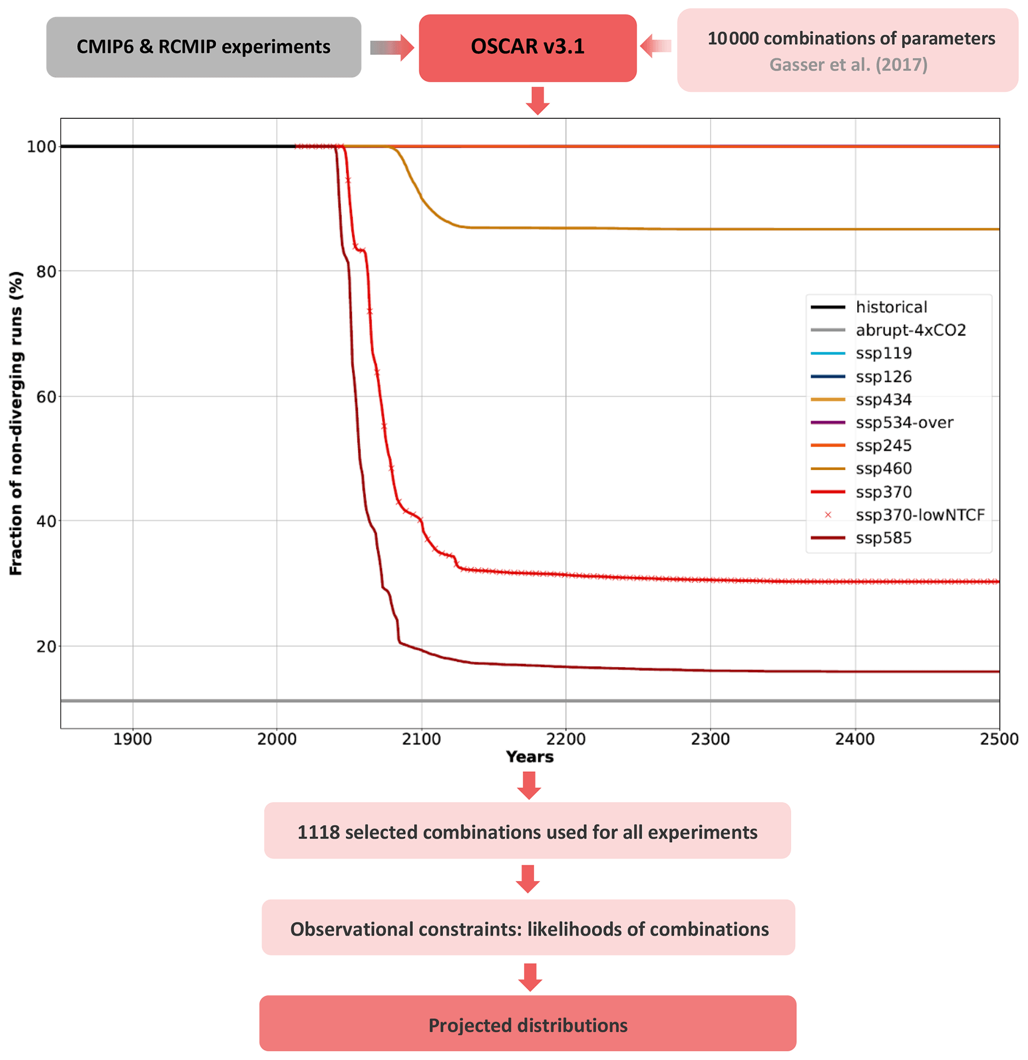
Figure A1 Conceptual description of the framework used in this study. The 10000 configurations drawn (Gasser et al., 2017) are used in OSCAR in a Monte Carlo setup for all experiments. The exclusions are based on their exceedance to thresholds in the ocean sink, land sink, CO₂ emissions from LUC and CO₂ emissions from permafrost. The remaining subset common to each experiment is then used for all. The likelihood of the configurations that are kept is then calculated (Gasser et al., 2020) and applied to all experiments.

To discard the unrealistic configurations, we use the experiments ssp585, ssp370, 1pctCO2 and abrupt-4xCO2 for their high warming over different timescales. We use the ocean sink, the land sink, the CO₂ emissions from LUC and the CO₂ emissions from permafrost to ensure that the whole carbon cycle remains within reasonable boundaries. The criteria are set based on the performance of the remaining subset. In general, we use 20 PgC yr⁻¹ in absolute values as a threshold for divergence. Over ssp585 and ssp370, the domain is restrained to strictly positive values, due to the additional mode mentioned previously. Over abrupt-4xCO2, the criteria are applied over the last 50 years of the experiments only. In 1pctCO2, the run is extended by another 100 years for better identification. Most of the exclusions are related to ocean carbon sink; the other variables only bring little exclusions. We keep the 1118 configurations not causing any divergences in all the experiments as a common set of configurations for all experiments.

The need for exclusion is stronger as the atmospheric concentration of CO₂ and the global surface temperature increase. We acknowledge that when a significant fraction of the configurations is excluded, confidence in our model's result is lowered, but such a limitation of the validity domain is inherent to reduced-complexity models. The model's results might as well depend on the set thresholds for exclusions. However, this bias is reduced through the constraining round because configurations with unrealistic carbon cycles receive a low likelihood.

We observed that in most cases, the reason of the exclusion is due to a diverging ocean sink. The ocean carbon cycle of OSCAR is its oldest module (Gasser et al., 2017) and should be redesigned for more stable behavior under high-warming scenarios. A possibility is to increase the number of sub-time steps in the oceanic carbon module to avoid this issue for a fraction of the configurations, but it comes at the expense of the computational cost of the model.

After this exclusion, the outputs of OSCAR are constrained using observations. As done for RCMIP phase 2 (Nicholls et al., 2021b), the objective of this constraining round is to use the flexibility and the probabilistic frameworks of the reduced-complexity models to synthesize lines of evidence with the modeling of the Earth system. With OSCAR, we assess the physical likelihood of the model's configurations using lines of evidence from the literature. For every constraint, we extend a method already used with OSCAR but with only one constraint (Gasser et al., 2020; Le Quéré et al., 2018b). We assume a distribution from which we derive the likelihood of every configuration, as illustrated in equation A1 of Gasser et al. (2020b). The product of the probabilities over the set of constraints is the final likelihood of the configurations.

As the first observational constraint, we choose the surface air–ocean blended temperature change over 2000–2019 with reference to 1961–1990, provided as an assessed range by RCMIP (Nicholls et al., 2021b) from the HadCRUT 4.6.0.0 data set (Morice et al., 2012). This constraint is meant to provide information on the climate system. To constrain the carbon cycle, we use compatible fossil-fuel emissions. For now, OSCAR v3.1 is calibrated on CMIP5, which motivates the use of the compatible emissions of CMIP5, not those of CMIP6. An initial set of constraints based solely on observations had revealed that using projections helped the overall constraining round, thanks to the larger perturbation in the scenarios than in the historical period. Thus we choose the CMIP5 cumulative compatible fossil-fuel emissions over the concentration-driven historical simulation and four RCPs (Ciais et al., 2013b). To further constrain the partitioning of the carbon sinks between land and ocean, we use data on the cumulative net ocean to atmosphere flux of CO₂ over 1750–2011 (Ciais et al., 2013b).

Appendix B: Behavior of OSCAR

B1 Carbon geoengineering

B1.1 Idealized experiments

Experiments of CDRMIP are designed to investigate the consequences of carbon dioxide removal for the Earth system (Keller et al., 2018). In 1pctCO2-cdr, the atmospheric CO₂ increases by 1 % every year (just like 1pctCO2), but after 140 years, the atmospheric CO₂ decreases following a pathway at the same rate as in the ramp-up period. Once CO₂ has returned to its preindustrial state, the experiment is extended over 1000 years. As shown in Fig. B1, the GSAT reaches 3.68±0.39 K at the end of the ramp-up forcing, and it goes back to 0.85±0.22 K at the end of the ramp-down forcing. For all variables, such as the CH₄ emissions from wetlands, removing CO₂ from the atmosphere during ramp-down effectively reduces the perturbation in the variable that was induced by the ramp-up, albeit within a different time frame that is typical of a dynamic hysteresis (Boucher et al., 2012). Once the global temperature change is sufficiently reduced, the permafrost carbon stock slowly reconstitutes itself as well. However, the whole Earth system is not fully recovered as soon as the preindustrial level of atmospheric CO₂ is reached. To return within 10 % of the maximum perturbation at the end of the CO₂ ramp-up, it takes GSAT an average 110 extra years and the land carbon stock an average 26 years. At the end of the 1000-year extension, the oceanic carbon stock remains at about 19 % of its maximum perturbation.

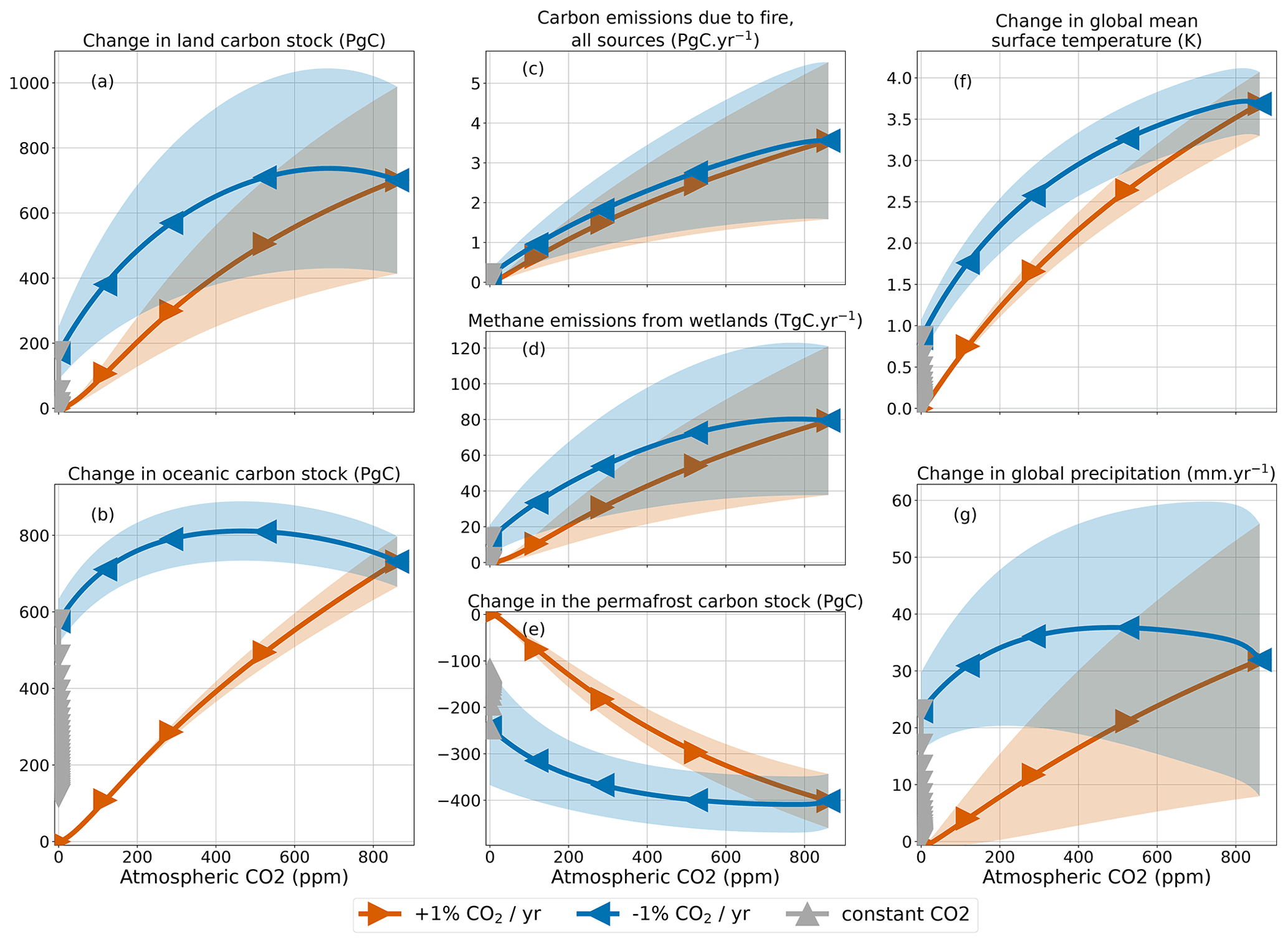
Figure B1 Reversibility experiment from CDRMIP. The orange lines correspond to the ramp-up of 1pctCO2-cdr, the blue line to its ramp-down and the grey line to the 1000 years with constant atmospheric CO₂. The plain lines are the averages, and the shaded areas represent ±1 standard deviation ranges.

Other CDRMIP experiments based on pulses of carbon emission or removal in an emission-driven configuration were performed to evaluate the response of the Earth system to CDR. These experiments are used to calculate the absolute global warming and temperature potentials (AGWPs and AGTPs) of CO₂, which serve to establish the global warming and temperature potentials (GWPs and GTPs) of other greenhouse gases (Myhre et al., 2013). In esm-pi-CO2pulse, a 100 PgC pulse is emitted from the preindustrial environmental condition in 1860, whereas 100 PgC is removed in esm-pi-cdr-pulse. In esm-yr2010CO2-CO2pulse, the 100 PgC pulse is applied in 2015 but under 2010 environmental conditions, whereas this 100 PgC is removed on the same date in esm-yr2010CO2-cdr-pulse. We calculate time series of AGWPs and AGTPs under these experiments (Fig. B2). The differences to the reference pulse are shown in a different panel for clarity. We pinpoint that, just like the other experiments, we are calculating these potentials with the interactive permafrost of OSCAR. The larger source of differences lies in the background: under preindustrial environmental conditions, emission pulses have a stronger AGWP or AGTP over the short term, but this is inverted over the longer term. Over the short term, this is due to the logarithmic expression of the CO₂ radiative forcing that is less saturated under preindustrial conditions. Over the long term, this is due to the deterioration of the carbon sink capacities under current conditions (Raupach et al., 2014). Similar reasons explain why a pulse of carbon removal cools the atmosphere slightly more over the short term than a pulse of emission warms it but less over the long term. Our results cannot be compared to the final CDRMIP results yet, for they are unpublished, but they are consistent with those obtained with a model of intermediate complexity (Zickfeld et al., 2021).

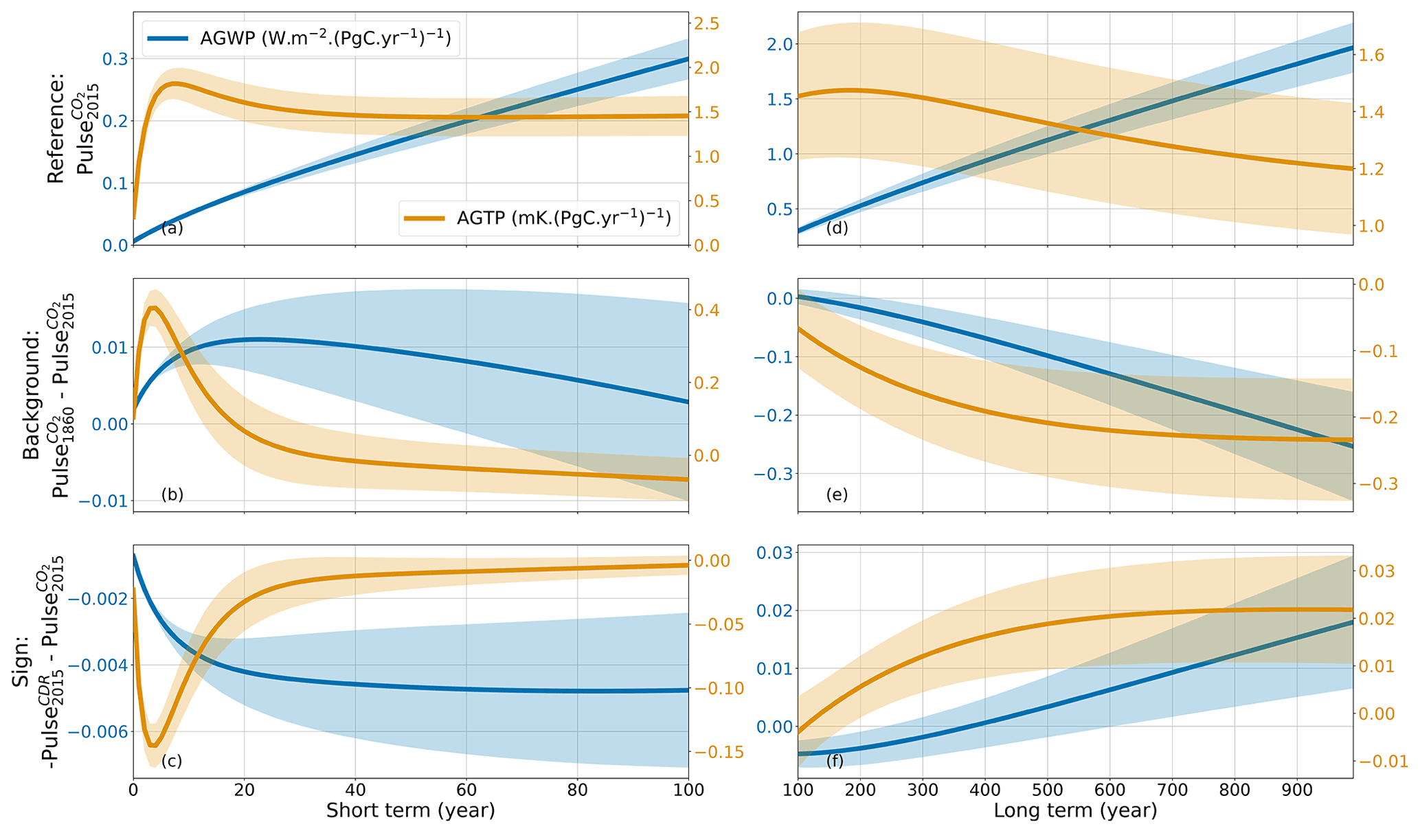
Figure B2 AGWP (blue) and AGTP (orange) of CO₂ for 100 PgC of CO₂ emissions under actual environmental conditions. The dependency of this reference on a change of background is on the second line. The dependency on the sign of the pulse, emissions or removal is on the third line. The lines are the averages, and the shaded areas represent ±1 standard deviation ranges.

B1.2 Alternative scenarios

The C4MIP (Jones et al., 2016) experiments ssp534-over-bgc and ssp585-bgc differ from ssp534-over and ssp585 in that the prescribed CO₂ does not affect the total radiative forcing, thus causing a lower change in GSAT and maintaining a relatively high carbon sinks efficiency. Figure B3 shows both carbon sinks under the variants and the base scenarios. Note that the -bgc experiments stem from a different historical simulation (hist-bgc). Under the high-warming scenarios ssp585, climate change reduces the oceanic carbon sink by 1.93±0.69 PgC yr⁻¹ and the net land carbon flux by 4.31±1.93 PgC yr⁻¹ in 2100. Under the overshoot scenario ssp534-over, this difference is lower, owing to its declining atmospheric CO₂. Removing the impact of climate change on the carbon cycle increases the land carbon stock by 269±52 PgC in ssp534-over but by 501±117 PgC in ssp585 in 2100, due to the higher warming in the latter case. We note that the permafrost carbon stock drives most of the changes because if permafrost is ignored in the bgc variant, these changes are reduced to 57±32 and 131±77 PgC in ssp534-over and ssp585 respectively.

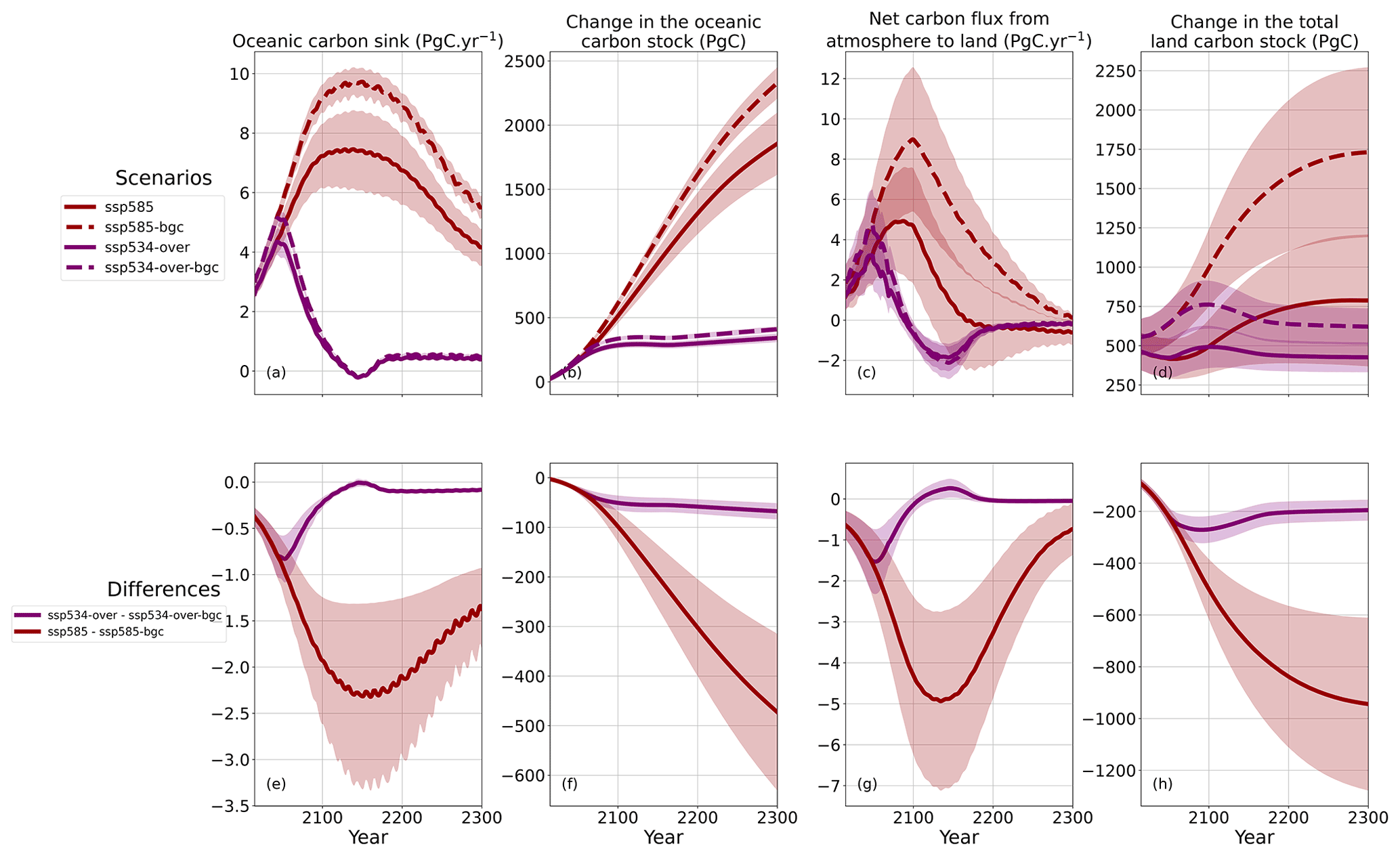
Figure B3 Effect of climate change on the carbon cycle in the scenarios ssp534-over and ssp585. The net flux from atmosphere from land is the sum of the land carbon sink, CO₂ emissions from land-use and land-cover change, and CO₂ and CH₄ emissions from permafrost. The changes in the total land carbon stock include those in the permafrost. Note that the increased uncertainty in the ocean sink before 2250 is an artifact of our exclusion procedure (see text on post-processing) that cannot capture the Monte Carlo members that already started diverging. Extensions are shown only up to 2300. The lines are the averages, and the shaded areas represent ±1 standard deviation ranges.

B2 Solar geoengineering

B2.1 Idealized experiments

Experiments of GeoMIP (Kravitz et al., 2015) are designed to investigate the geoengineering techniques of solar radiation management (SRM). Although OSCAR is not suited for all GeoMIP experiments, as it lacks any spatially resolved process, a few simulations remained accessible to our model. We run experiments G1 and G2: G1 essentially follows abrupt-4xCO2, albeit with a changed incoming solar radiation that compensates for the radiative forcing caused by the increasing atmospheric CO₂. For G2, an identical principle is applied but using 1pctCO2 as a basis. As explained by Kravitz et al. (2011), the change in solar radiation compensates solely for the radiative forcing of CO₂. However, it does not compensate for other radiative effects introduced by biogeochemical feedbacks, such as the fertilization by CO₂, affecting the carbon cycle, thus changing biomass burning emissions. Figure B4 shows that offsetting the CO₂ radiative forcing with a change in solar activity effectively compensates for the change in GSAT. However, we simulate the GSAT decreases in G1 and G2 to reach $-\mathrm{0.08}\pm \mathrm{0.20}$ and $-\mathrm{0.07}\pm \mathrm{0.20}$ K, respectively, at the end of simulations. The compensation of the sole radiative forcing of CO₂ does not balance out other feedbacks. There remains an additional radiative forcing, mostly due to changes in aerosols (as also shown in Fig. 3), which results in this relatively small cooling in G1 and G2. We estimate that in OSCAR about half of this effect is caused by the vegetation being fertilized by CO₂, fueling increased natural biomass burning emissions, and the remaining half is caused by the direct impact of GSAT on the atmospheric lifetime of aerosols (not shown). We note that the latter effect could be poorly estimated, in these specific experiments, as OSCAR's formulation for the lifetime of aerosols depends only on GSAT and not on the precipitation intensity.

Indeed, global precipitation does not respond in a similar way because changes in atmospheric CO₂ and solar radiation have a different impact of the hydrological cycle (Andrews et al., 2010). In spite of a fully compensated for GSAT change, global precipitation is significantly reduced in G1 and G2, showing that such a SRM technique does not entirely negate climate change. This demonstrates that OSCAR is capable of reproducing this well-established effect of this SRM technique (Boucher et al., 2013). One added value of having a fully coupled ESM run these GeoMIP experiments is that we can also provide an estimate of the impact of the SRM technique on the carbon cycle. Figure B4 also shows that the land and ocean carbon stocks are increased in G1 and G2, respectively by about 33 % and 20 % at the end of the simulations, owing to the loss of carbon sink efficiency that is avoided by maintaining the temperature to its preindustrial level.

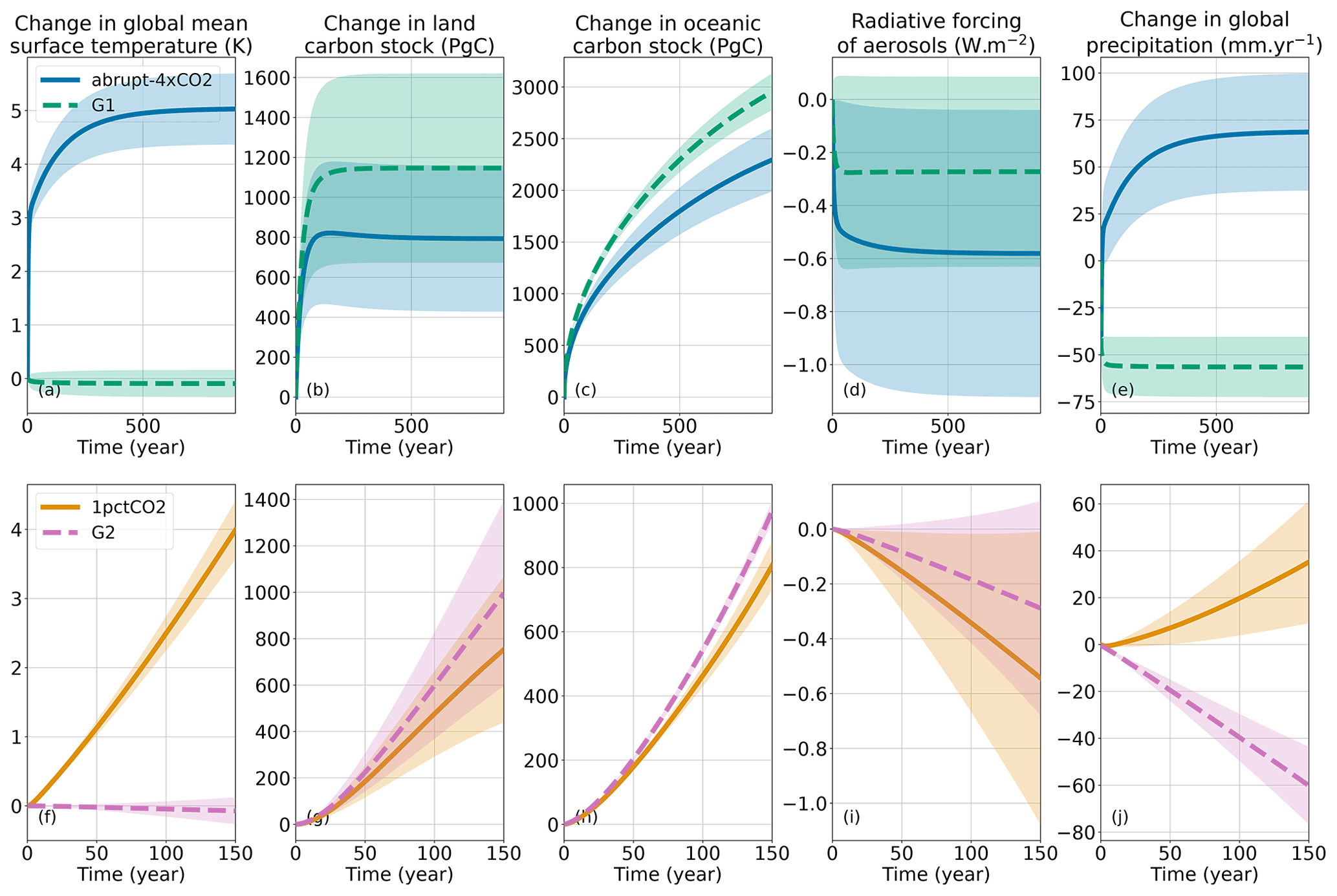
Figure B4 Experiments from GeoMIP compared to their DECK counterpart. The plain lines are the averages, and the shaded areas represent ±1 standard deviation ranges.

B2.2 Alternative scenarios

In addition to the few idealized experiments of GeoMIP (Kravitz et al., 2015) that are accessible to OSCAR, one scenario variant focusing on SRM was also feasible. The G6solar experiment stems from ssp585, but the solar constant changes from 2020 onwards to compensate the radiative forcing of ssp585 and match the one of ssp245. As shown in Fig. B5, differences remain although the GSAT of G6solar decreases to a level comparable to ssp245. We calculate the change in solar constant as the difference from the radiative forcing of ssp245 to ssp585. By construction, it excludes feedbacks caused by this change and does not fully cancel the change in global precipitation, just like in G1 and G2. Consequently, the carbon stocks still increase in G6solar, even more than in ssp585 thanks to the lower GSAT and despite lower global precipitation.

Figure B5 Effect of introducing SRM in the SSP5-8.5 to reach the SSP2-4.5. The lines are the averages, and the shaded areas represent ±1 standard deviation ranges.

B3 Land use

B3.1 Alternative historical simulations

LUMIP consists of experiments specifically focusing on land-use activities, and most of them are run by the Earth system models in a so-called “offline” fashion (Lawrence et al., 2016). It means that a reconstruction of past climate variables GSWP3 (Lawrence et al., 2016; van den Hurk et al., 2016) is prescribed to the model, so that the land module is actually decoupled from the rest of the model. Despite its simplicity, OSCAR has an added value in running those simulations, as it embeds a book-keeping module that endogenously estimates CO₂ emissions from land-use and land-cover change. The main land carbon fluxes and stocks simulated under the reference experiment (dubbed land-hist) are shown in Fig. B6, along with three sets of sensitivity experiments described hereafter. The results are similar to those obtained recently with the same version of the model but with slightly differing forcings and a different constraint (Gasser et al., 2020). The simulated land carbon stock decrease up to the 1970s because of land-use activities emitting more CO₂ than the sink absorbs thanks to CO₂ fertilization and other factors. The carbon stock of 2010 is higher than the one of 1850 by only 1±42 PgC. For comparison, for 1850–2014 the GCB 2020 provides a net budget for the land sink and CO₂ emissions from LUC of $-\mathrm{5}\pm \mathrm{90}$ PgC (Friedlingstein et al., 2020).

Figure B6 Land-use experiments from LUMIP. The first row of the figure corresponds to the reference experiment (land-hist) while other rows show sensitivity experiments as a difference to land-hist. land-hist-altStartYear is shown only from 1850 despite starting in 1700. The lines are the averages, and the shaded areas represent ±1 standard deviation ranges.

The experiments land-cCO2 and land-cClim are used to disentangle the contribution of CO₂ fertilization and changing climate on the land carbon cycle. In land-cCO2, the atmospheric CO₂ is constant and set to the preindustrial value. In land-cClim, the climate drivers loop over the year 1901–1920 of the data set, thus simulating a preindustrial climate. Figure B6 shows the differences; for example, land-hist − land-cCO2 illustrates the effect of atmospheric CO₂ on the variables of interest. Thanks to these experiments, we show that CO₂ is the main driver of the land sink in OSCAR, driving most of the trend, with climate bringing a significant interannual variability but virtually no trend, except over the recent past. In 2010, climate caused a small difference of $-\mathrm{10}\pm \mathrm{10}$ PgC in total land carbon stock, while CO₂ caused one of 141±42 PgC. This has to be balanced with the results of the C4MIP idealized experiments, where we saw OSCAR is less sensitive to climate change than CMIP5 models. Additionally, we see that the effect of climate and CO₂ on land-use and land-cover change emissions is minor, which is consistent with the fact that they are firstly determined by preindustrial carbon densities (Gasser et al., 2020; Gasser and Ciais, 2013).

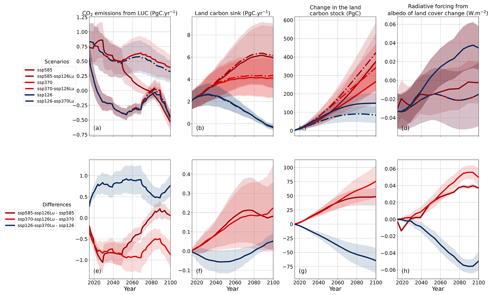
Figure B7 Effect of alternative land-use and land-cover change drivers in the scenarios ssp126, ssp370 and ssp585. Here, the changes in the land carbon stock do not include the changes in the permafrost. The lines are the averages, and the shaded areas represent ±1 standard deviation ranges.

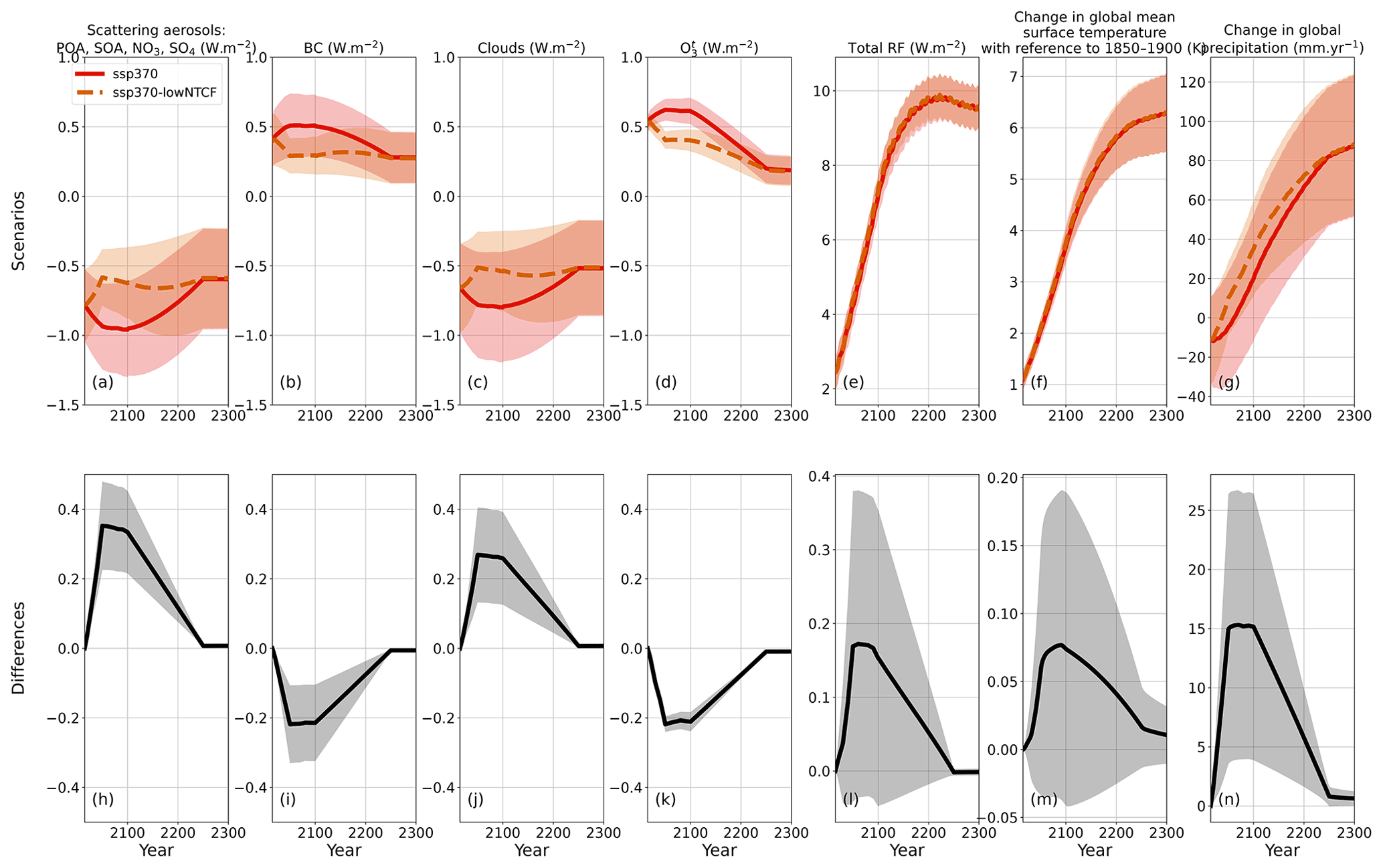
Figure B8 Effect of lower NTCF emissions in the SSP3-7.0. Extensions are shown only up to 2300. The lines are the averages, and the shaded areas represent ±1 standard deviation ranges.

A second set of experiments is meant to investigate the impact of land-use practices. Land-cover change contributed $-\mathrm{152}\pm \mathrm{44}$ PgC to the 2010 change in land carbon stock from 1850, which corresponds to most of the total land-use and land-cover change emissions. Notably, it also reduced the land sink – an effect called the loss of additional sink capacity that has been diagnosed and quantified with OSCAR in the past (Gasser et al., 2020; Le Quéré et al., 2018b; Gasser and Ciais, 2013; Friedlingstein et al., 2020). Shifting cultivation (i.e. rapidly rotating land-use change between agriculture and natural ecosystems) had a relatively low impact on CO₂ emissions, leading to a change in land carbon stock of $-\mathrm{8}\pm \mathrm{2}$ PgC at the end of the simulation in 2010. Similarly, wood harvest (in woody ecosystems that do not see land-cover change) had an overall impact of $-\mathrm{16}\pm \mathrm{4}$ PgC. Both shifting cultivation and wood harvest have no impact at all on the land sink, by construction of their formulation in OSCAR (Gasser et al., 2020). Finally, the effect of having cropland-specific parameters in the model is isolated thanks to the land–crop–grass experiment, in which new croplands are treated as grasslands. Having grasslands instead of croplands increases both the land sink and the CO₂ emissions from land-use and land-cover change, resulting in a land carbon stock that is higher by 31±26 PgC. All these values are entirely in line with an existing assessment of those land-use practices in which an earlier version of OSCAR took part (Arneth et al., 2017).

The third set of experiments relates to varying input data sets of land-use and land-cover change drivers. Two of these (land-hist-altLu1 and land-hist-alLu2) relied on the two variations of the main LUH2 data set known as the “high” and “low” variants (respectively) (Hurtt et al., 2020). We find that the so-called low variant leads to slightly higher land-use and land-cover change emissions, amounting to a land carbon stock that is lower by 8±2 PgC over the whole period. The high variant produces slightly lower total emissions, leading to a land carbon stock that is higher by 17±5 PgC. Neither variant has a significant impact on the land sink. According to the description of these two variations (Hurtt et al., 2020), they differ from the default data set mostly in the harvest of biomass and are very similar from 1920 onwards. The last LUMIP experiment run with OSCAR is one that uses the primary data set but an alternative starting year (land-hist-altStartYear). This required making an additional spin-up of the model under the environmental conditions and land cover of the year 1700. Compared to the reference experiment, we find a slightly higher land sink after 1850 that decreases through time, owing to the ecosystems not being at a steady state on that date. Similarly, emissions are slightly higher, but the difference to the reference case tends towards zero as the legacy of land-use and land-cover change prior to 1850 fades away. The land carbon stock in 2010 is dominated by the increased land sink and amounts to a small increase of $-\mathrm{17}\pm \mathrm{13}$ PgC in the land. Comparing the latter value with the total change in land carbon in the reference experiment suggests that starting simulations in 1850 instead of 1700 or 1750 introduces a non-negligible bias in the CMIP6 exercise.

Figure B9 Comparison between RCPs (CMIP5) and SSPs (CMIP6). The lines are the averages, and the shaded areas represent ±1 standard deviation ranges.

B3.2 Alternative scenarios

LUMIP introduced variants of regular scenarios in which alternative land-use and land-cover change drivers coming from another scenario are prescribed (Lawrence et al., 2016), some of which being used in CDRMIP to assess afforestation (Keller et al., 2018). Two such experiments are the pessimistic ssp585 and ssp370 combined with the land-use activities of the optimistic ssp126 (named ssp585-ssp126Lu and ssp370-ssp126Lu, respectively). A third experiment consists in using the land-use of ssp370 but under ssp126 (named ssp126-ssp370Lu). Comparisons of these experiments with their regular counterparts are shown in Fig. B7. As expected, changing the land-use scenario roughly replaces one SSP's land-use emissions by another's, albeit with some slight differences in the later stage of the simulations (i.e. after 2050) when atmospheric CO₂ and climate are significantly different from the reference scenario's, which has an impact in OSCAR because of transiently changing land carbon densities. The effect on the land carbon sink is also quantified, showing that sink capacity can be preserved by conserving natural ecosystems, although it remains a relatively small effect in absolute value. We note that the ability of properly isolating both effects (on land-use emissions and on the sink) is a specific feature of OSCAR that stems from the formulation of its land carbon cycle (Gasser et al., 2020; Gasser and Ciais, 2013), and we do not expect many complex ESMs to be able to provide such a partitioning. The overall effect on land carbon stock change in 2100 is 48±15, 76±28 and $-\mathrm{65}\pm \mathrm{23}$ PgC, in the ssp585-ssp126Lu, ssp370-ssp126Lu and ssp126-ssp370Lu scenarios respectively. While the land carbon stocks are affected, the change in land cover also affects the planetary albedo. The radiative forcing from albedo of land-cover change is exchanged between ssp126 and ssp370, but changes remain below 0.1 W m⁻². The net combined effect on projected temperature cannot be estimated because these experiments are concentration-driven.

B4 Alternative scenarios for NTCFs

The ssp370-lowNTCF scenario is a variant of the ssp370 differing by its lower emission of short-lived pollutants affecting the RF of NTCFs. As illustrated in Fig. B8, the variant leads to a somewhat equivalent warming, although with very slightly less cooling from NTCFs. This almost negligible effect on global temperature is actually the result of two large but compensating effects that manifest the most between 2050 and 2100. The lower emission of warming NTCFs leads to absorbing aerosols (i.e. BC) warming less by $-\mathrm{0.21}\pm \mathrm{0.11}$ W m⁻² and tropospheric ozone warming less by $-\mathrm{0.21}\pm \mathrm{0.03}$ W m⁻² in 2100. Conversely, it also leads to scattering aerosols cooling less by 0.33±0.12 W m⁻² and the indirect aerosol effects cooling less by 0.26±0.13 W m⁻² at the same date. This results in a small increase of the total radiative forcing of 0.15±0.20 W m⁻² and a GSAT change of only 0.07±0.11 K. However, the difference in forcing agents between the two scenarios leads to a significant change in global precipitation that reaches 15±11 mm yr⁻¹ in 2100. The change in precipitation is consistent with our results for the GeoMIP experiments and what we know of the global water cycle (Shine et al., 2015).

B5 Comparison of two generations of scenarios

Initially, the SSPs scenarios were designed to reach the RF of RCPs in 2100, to provide a common grid for reading and comparing all the SSPs scenarios. Hence, the same four RF targets chosen in CMIP5 with the RCPs (2.6, 4.5, 6.0 and 8.5 W m⁻²) have also been chosen in CMIP6 with four out of the eight SSPs used. Yet, CMIP6 ESMs did not run RCPs because these scenarios are not part of the CMIP6 experiments. Therefore, the difference between RCP projections in CMIP5 and SSPs projections in CMIP6 under the same RF targets are due to both a change in the generation of ESMs and a change in scenarios. In Fig. B9, we represent both RCPs and SSPs under the same version of OSCAR, showing the difference due to the sole change in scenarios. These scenarios use different drivers, as illustrated by the atmospheric CO₂ prescribed to these concentration-driven experiments, usually with higher CO₂ concentrations in the CMIP6 version. Except for the 8.5 target, the RF also tends to be higher in the CMIP6 version, compared to the CMIP5 version, meaning changes in other drivers are not enough to balance the CO₂ increase. While the 2.6 and 8.5 W m⁻² targets are reached in 2100, the 4.5 and 6.0 W m⁻² are not. However, our results can be compared to those of MAGICC in these two cases (IIASA, 2018b), and both reduced-complexity models are consistent. Because of the similar RF targets, GSAT are relatively similar over the 21st century, but RCPs and SSPs tend to dissociate later on. In 2300, moving from RCPs to SSPs changes GSAT by 18±8 %, 9±3 %, 5±2 % and $-\mathrm{6}\pm \mathrm{1}\mathit{\%}$ in the four tested scenarios, respectively. Differences in other key variables such as the carbon sinks logically respond to these differences in atmospheric CO₂ and global temperature change, as also shown in Fig. B9.