The IPCC Sixth Assessment Report WGIII climate assessment of mitigation pathways: from emissions to global temperatures

While the Intergovernmental Panel on Climate Change (IPCC) physical science reports usually assess a handful of future scenarios, the Working Group III contribution on climate mitigation to the IPCC's Sixth Assessment Report (AR6 WGIII) assesses hundreds to thousands of future emissions scenarios. A key task in WGIII is to assess the global mean temperature outcomes of these scenarios in a consistent manner, given the challenge that the emissions scenarios from different integrated assessment models (IAMs) come with different sectoral and gas-to-gas coverage and cannot all be assessed consistently by complex Earth system models. In this work, we describe the “climate-assessment” workflow and its methods, including infilling of missing emissions and emissions harmonisation as applied to 1202 mitigation scenarios in AR6 WGIII. We evaluate the global mean temperature projections and effective radiative forcing (ERF) characteristics of climate emulators FaIRv1.6.2 and MAGICCv7.5.3 and use the CICERO simple climate model (CICERO-SCM) for sensitivity analysis. We discuss the implied overshoot severity of the mitigation pathways using overshoot degree years and look at emissions and temperature characteristics of scenarios compatible with one possible interpretation of the Paris Agreement. We find that the lowest class of emissions scenarios that limit global warming to “1.5 ^∘C (with a probability of greater than 50 %) with no or limited overshoot” includes 97 scenarios for MAGICCv7.5.3 and 203 for FaIRv1.6.2. For the MAGICCv7.5.3 results, “limited overshoot” typically implies exceedance of median temperature projections of up to about 0.1 ^∘C for up to a few decades before returning to below 1.5 ^∘C by or before the year 2100. For more than half of the scenarios in this category that comply with three criteria for being “Paris-compatible”, including net-zero or net-negative greenhouse gas (GHG) emissions, median temperatures decline by about 0.3–0.4 ^∘C after peaking at 1.5–1.6 ^∘C in 2035–2055. We compare the methods applied in AR6 with the methods used for SR1.5 and discuss their implications. This article also introduces a “climate-assessment” Python package which allows for fully reproducing the IPCC AR6 WGIII temperature assessment. This work provides a community tool for assessing the temperature outcomes of emissions pathways and provides a basis for further work such as extending the workflow to include downscaling of climate characteristics to a regional level and calculating impacts.

1 Introduction

The Working Group III (WGIII) contribution to the Intergovernmental Panel on Climate Change (IPCC) Sixth Assessment Report (AR6) assesses the recent literature on how climate change can be mitigated (IPCC, 2022c). A key part of this assessment uses emissions scenarios (Riahi et al., 2022) that explore a variety of climate change mitigation futures. The Paris Agreement, which specified a long-term global temperature goal (UNFCCC, 2015), strengthened by the Glasgow Climate Pact stressing the 1.5 ^∘C temperature level (UNFCCC, 2021), made it ever more relevant to determine global mean surface temperature outcomes in assessments of policy-relevant climate mitigation literature. Until now, the climate-assessment process utilised by the IPCC has been described in the report but never discussed in detail or been made openly available to the community as a software tool. Making the climate-assessment process open-source will not only facilitate the reproducibility of the report's scientific findings, but also facilitate future analyses of new data applying a methodology consistent with the AR6 WGIII report.

In this paper, we (a) lay out and discuss the methodology used in IPCC AR6 for assessing the global warming implications of scenarios with sufficient emissions quantifications, (b) describe the global mean temperature outcomes of the scenario set available in the AR6 WGIII report's scenarios database (AR6DB; Byers et al., 2022), and (c) document and link to the tools used for this part of the assessment. These temperature projections from integrated assessment model (IAM) scenarios are used across many parts of the WGIII report. The methodology described in this paper was used in a few sections in the Summary for Policymakers (SPM) (IPCC, 2022d), and especially in Chapter 3 on Mitigation Pathways Compatible with Long-Term Goals (Riahi et al., 2022). The description provided here gives further detail on the summary of the methods and analysis already available in Annex III of AR6 WGIII on Scenarios and Modelling Methods (IPCC, 2022a).

A comprehensive assessment of the global temperature outcomes of long-term greenhouse gas (GHG) emissions scenarios requires diverse emissions data to be made comparable, gaps in data to be completed, and tools to project global temperature from those emissions that reflect the best available climate science knowledge. After a selection of scenarios that comply with reporting standards and are within ranges of uncertainty (“vetting”) is made, global mean temperature outcomes are calculated. The climate-assessment workflow we describe here has three core steps: (1) harmonisation of emissions, (2) infilling of emissions, and (3) running of one or several emissions-driven reduced-complexity climate models (see Fig. 1).

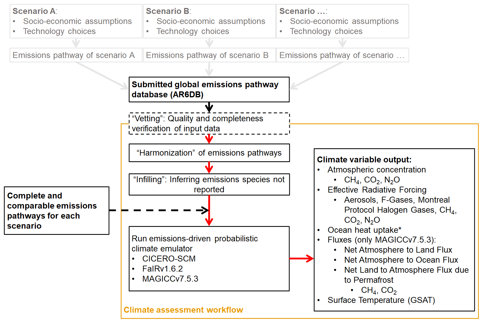
Figure 1 The steps of the “climate-assessment workflow”. Overview of climate-assessment processing steps applied in the Working Group III contribution to the IPCC Sixth Assessment Report. The asterisk is added in the figure to indicate that ocean heat uptake was provided only by FaIRv.1.6.2 and MAGICCv7.5.3 in AR6.

In the harmonisation process, scenarios are made comparable by ensuring they start from the same historical emission levels. This ensures that differences between climate futures resulting from two different pathways are the result of future emissions due to structural changes in mitigation scenarios rather than different historical emissions estimates or assumptions.

In the infilling step, data gaps in the emissions scenarios, such as time evolutions for some individual gas or aerosol species that are not reported by a given IAM, are closed by inferring representative trajectories of those missing species from the wider literature.

In the climate run step, reduced-complexity climate models (also known as climate emulators) are used to project the physical climate response to emissions. These climate emulators are calibrated to closely reproduce historically observed warming, projections of warming for standard scenarios, and the uncertainty ranges in key physical climate parameters assessed in the IPCC Working Group I (WGI) report (IPCC, 2021a). This close collaboration between WGI and WGIII to ensure consistency of climate assessments across various IPCC AR6 products is a key development compared to the IPCC Fifth Assessment Report (AR5) (IPCC, 2014, 2013) and earlier IPCC assessment reports. The AR6 WGIII report is the first IPCC report that uses climate emulators that are fully in line with complex models and other lines of evidence as assessed by the physical science basis of the same cycle.

A total of 3131 global and regional scenarios were submitted to the AR6 Scenario Explorer hosted by IIASA (Byers et al., 2022). Out of this set, 1686 global scenarios were considered to meet minimum quality standards for use in long-term scenario assessment based on the vetting criteria as set out in Annex III of IPCC WGIII. This set was further narrowed down to 1202 scenarios (IPCC, 2022a) that contained sufficient emissions data across gases and sectors to provide full-century climate outcomes. This sub-selection to more complete scenarios ensures that the harmonised and infilled emissions reflect the intention of the prospective modelling in the original scenario submission. For the main text, figures, and tables in this paper, we use this set of 1202 scenarios. While most of these scenarios contain regional emissions pathways, WGIII AR6 only assessed global climate variables based on global emissions estimates, which is the common level that the used climate emulators operate on. This means that evaluating the regional effects of for instance regional aerosol emissions is beyond the scope of this assessment, having as a primary aim the assessment of global mean surface temperature change.

In the remainder of this paper, we start by placing the IPCC WGIII AR6 infilling steps, harmonisation procedures, and climate assessment in their historical context and present the criteria they aimed to meet. Then, we provide details on the methods applied, going from emissions provided by IAMs to outputs from climate emulators. Lastly, we touch upon future development options.

2 History of scenario temperature projections in IPCC WGIII reports and the updated process in AR6

2.1 History of climate-assessment processes

2.1.1 Climate emulators in IPCC reports

Climate emulators have been used by the IPCC from its very start. For instance, the First Assessment Report explains that “simpler models, which simulate the behaviour of [general circulation models (GCMs)], are also used to make predictions of the evolution with time of global temperature from a number of emission scenarios. These so-called box-diffusion models contain highly simplified physics but give similar results to GCMs when globally averaged.” (IPCC, 1992). Emulators, because of their computational simplicity, can be used much more widely than complex GCMs or Earth system models (ESMs).

Because of the limited ability in the 1990s to perform long-term coupled atmosphere–ocean runs with a broad coverage of different GHGs and aerosols and an interactive carbon cycle, the early assessment reports relied heavily on simple climate models, including the WGI reports. A technical overview report about their strength and limitations was published by the IPCC in 1997 (Houghton et al., 1997). With an increasing availability of Earth system models of intermediate complexity (EMICs), coupled atmosphere–ocean general circulation models (AOGCMs), and ultimately the fully fledged ESMs, the focus shifted in the physical WGI reports towards the use of progressively more complex models. However, in the AR6 WGI report, climate emulators were used to fill in gaps from experiments of interest that are not run by ESMs (e.g. SPM Figs. 2c and 4b, IPCC, 2021b) and also to bridge the gap between expert assessment of the climate system and some of the unconstrained projections resulting from ESMs (Hausfather et al., 2022; Lee et al., 2021; Forster et al., 2021). Multiple lines of evidence in support of the assessment of climate sensitivity and other climate characteristics led to IPCC WGI AR6 adopting a new approach, which also involved calibrating climate emulators to translate the assessment of key climate characteristics into the global mean temperature projections. Additionally, the increased focus on translating insights from WGI to other stakeholders and scientific communities included stronger cross-WG collaboration and triggered a concerted effort for climate emulator calibration on the basis of a wide range of WGI assessment results.

Figure 2 Summary statistics (a: emissions, b: atmospheric concentrations, c: global mean surface temperature) over time across all scenarios in the AR6DB that received a temperature classification and across scenarios in AR6 temperature categories C1 and C3. Panel (a) shows emissions as modelled by IAMs (“Native”), after harmonisation (“Harmonized”), and after infilling missing reported emissions (“Infilled”). Panel (b) and panel (c) show climate outcomes per climate model, using the median value of each variable from the climate emulator probabilistic distributions.

In the WGIII report, there are two key reasons for using climate emulators to assess the temperature outcomes of long-term climate mitigation scenarios. The first reason is time and resources. With a large number of scenarios available from a wide variety of studies, it would take too much computing time to rapidly simulate all scenarios with one ESM, let alone with a wider set of models such as those that participate in international initiatives like the Coupled Model Intercomparison Project (CMIP). For instance, a quick turnaround was required between WGIII's literature cut-off date (11 October 2021), by which scenarios had to be confirmed as published, and WGIII's deadline for Final Government Draft submission by authors (1 November 2021). It is computationally not feasible for modern ESMs to run all scenarios in this timespan. Typically, an IPCC report undergoes multiple expert and government reviews. This means that the climate assessment is repeated multiple times over the course of an IPCC report drafting cycle, which for WGIII AR6 took 3 years from the first lead author meeting to the approval of the SPM. The second reason mirrors the reasoning in WGI, i.e. using climate emulators to combine multiple lines of evidence to represent the overall best estimate and uncertainty range (Lee et al., 2021). In the WGIII context, a single ESM, or even a set of them, is unlikely to match the best estimate as well as physical climate uncertainty of the assessed temperature response to anthropogenic emissions with a good representation of uncertainty as assessed by WGI and might not even reproduce historically observed global mean temperatures well (Smith and Forster, 2021).

2.1.2 Long-term mitigation pathway assessments in previous IPCC WGIII reports

This exercise sits within a tradition of large-scale assessments and previous IPCC WGIII reports, though the practice of grouping mitigation scenarios based on climate emulator outcomes is more recent. Using two models, the First Assessment Report (FAR) WGIII (IPCC, 1990) evaluated three mitigation scenarios (SA90) and two reference scenarios, calculating their atmospheric CO₂ and CO₂-equivalent concentrations, but did not directly assess global temperature outcomes related to these scenarios. The 1992 supplement to the FAR (IPCC, 1992) evaluated six alternative emissions scenarios (IS92 a–f) and provided global warming estimates using the best estimate of climate sensitivity available at that time. In a 1994 follow-up report, the radiative forcing characteristics of the IS92 pathways were assessed in much more detail (IPCC, 1994). The Second Assessment Report (SAR; IPCC, 1996) assessed a wider range of socio-economic scenarios and used a more extensive set of simple climate models (Houghton et al., 1997) but did not use these to assess the temperature implications of the mitigation scenario literature. In a similar fashion, WGIII of the Third Assessment Report (TAR; IPCC, 2001) also did not perform its own temperature assessment or grouping of mitigation scenarios by climate categories but used CO₂ concentrations as stabilisation levels for the assessment of the mitigation pathways (e.g. SPM.1 and Table 2.6 in IPCC, 2001).

The WGIII Fourth Assessment Report (AR4; IPCC, 2007) contained the first IPCC temperature assessment of emissions scenarios from the available literature: 177 scenarios were assessed, covering a mix of CO₂-only and multi-gas studies. Scenario characteristics were compared by grouping them into six categories based on climate targets as reported in each of the original peer-reviewed articles assessed by the IPCC. Where data were unavailable, scenario characteristics for either CO₂ concentrations or radiative forcing within each category (15th and 85th percentiles) were derived using the relationship between CO₂ concentrations and radiative forcing and the relationship between CO₂ concentrations and equilibrium temperature. Only six scenarios fell into the lowest warming category, which was associated with 2.5–3.0 W m⁻² radiative forcing and CO₂ concentrations of 350–400 ppm in 2100, with a rough estimate of 2.0–2.4 ^∘C global mean surface temperature increase above pre-industrial levels (here referring to the era before the industrial revolution of the late 18th and 19th centuries, while in the rest of the paper “pre-industrial” refers to the period from 1850 to 1900) at equilibrium using a climate sensitivity of 3 ^∘C per doubling of CO₂ concentrations. The highest category covered the 6.0–7.5 W m⁻² range of forcing and featured only five scenarios. The report was clear about the limitation of this approach, writing in Sect. 3.3.5 that “it should be noted that the classification is subject to uncertainty and should thus be used with care” (IPCC, 2007).

In the Fifth Assessment Report (AR5) WGIII report (IPCC, 2014), a larger database of 915 scenarios was available for the assessment of mitigation pathways. These scenarios differed in their design (e.g. ever-growing emissions, climate stabilisation, or peak-and-decline scenarios) as well as in how many gases were included. Despite the methodological difficulties in comparing multiple types of scenarios, AR5 still grouped scenarios into different climate categories to enable comparison of their key characteristics (IPCC, 2014). With the scenario literature at that time often using 2100 radiative forcing targets to design scenarios, including the representative concentration pathways (RCPs), CO₂-equivalent concentrations in 2100 were chosen as a classification indicator (CO₂-equivalent concentrations represent the concentration of CO₂ that would cause the same radiative forcing as a given mixture of CO₂ and other forcing components). The calculation of CO₂-equivalent concentrations in 2100 from emissions was standardised. All scenarios with at least information on total Kyoto gas emissions were assessed using the climate emulator Model for the Assessment of Greenhouse Gas Induced Climate Change (MAGICC) version 6.3 (Meinshausen et al., 2011b, a). This model version drew on a probabilistic ensemble where concentration and radiative forcing outcomes were constrained by observations and physical climate parameter uncertainties assessed in AR4 (Meinshausen et al., 2009; Schaeffer et al., 2015), with model updates to better reflect the climate sensitivity distribution as assessed in AR5 WGI (Rogelj et al., 2012). To group scenarios, the median CO₂-equivalent concentration of total radiative forcing of this probabilistic ensemble was used. For emissions harmonisation, to avoid artefacts in the temperature projections resulting from differences in model-reported and historical emissions, emissions were set to historical observation values in 2010, with the difference from model-reported values linearly declining to zero in 2050 (Krey et al., 2014). At minimum, CO₂ from the energy and industrial processes (E&IP) sector (also known as CO₂ from the use of fossil fuels and industry or CO₂-FFI, as used in AR6) and CH₄ and N₂O from the E&IP and land use sectors from each individual scenario needed to be available. For emissions infilling of other species, a set of heuristics was applied to fill in any missing F-gases, carbonaceous aerosols, and/or nitrate emissions (Krey et al., 2014). Another set of practical heuristics was developed to classify scenarios that did not report all necessary GHGs and other emissions or did not report emissions until the end of the 21st century. The classification of such scenarios into groups was based on Kyoto gas forcing only (given a lack of total forcing) in 2100, cumulative CO₂ emissions from 2011 to 2100, and cumulative CO₂ emissions from 2011 to 2050, in order of preference; 114 scenarios were classified into the lowest category of 2.3–2.9 W m⁻² in 2100, with associated 2100 median temperatures ranging from 1.5 to 1.7 ^∘C above 1850–1900 levels.

The Special Report on Global Warming of 1.5 ^∘C (IPCC, 2018) – abbreviated as SR1.5 – featured an extensive climate assessment of emissions scenarios with the most advanced methods so far. After the introduction of temperature targets in international climate policy in the Cancún Agreement of 2010 (UNFCCC, 2010) and the subsequent adoption of the Paris Agreement with its specific long-term temperature goal as stated in Article 2 of the agreement (UNFCCC, 2015), SR1.5 was the first IPCC report where scenarios were categorised based directly on their projected global mean temperature outcomes. This temperature categorisation followed the practice established by the Emissions Gap Reports series of the UN Environment Programme (Hare et al., 2010; Rogelj and Shukla, 2012; Rogelj et al., 2011). SR1.5 only assessed scenarios with information until 2100 for at minimum CO₂ from E&IP and (total) CH₄, N₂O, and sulfur emissions. The SR1.5 approach used the same harmonisation method as AR5, but because an absolute offset harmonisation method would have turned some non-CO₂ emissions pathways negative, SR1.5 rather used a multiplicative (“ratio”) method (Forster et al., 2018). For the infilling of emissions species not reported, including F-gases and black carbon (BC), values from the low forcing scenario RCP2.6 (van Vuuren et al., 2011; Meinshausen et al., 2011a) were used, in line with the focus of the report on 1.5 and 2 ^∘C consistent scenarios. A total of 368 scenarios (out of 529 submitted scenarios) were grouped into six temperature categories, five of which were to indicate different categories of below 2 ^∘C scenarios (Forster et al., 2018; Rogelj et al., 2018: Tables 2.4 and 2.SM.12). Using a MAGICC6 set-up similar to that used in AR5 (Meinshausen et al., 2011b, a; IPCC, 2014), the temperature exceedance probabilities at peak temperature and in 2100 were used to define these categories. In addition, the climate emulator Finite Amplitude Impulse Response (FaIR) version 1.3 (Smith et al., 2018) was used to run all scenarios for a sensitivity analysis. FaIRv1.3 and MAGICC6 produced substantially different temperature and forcing levels for the same emissions scenarios, with FaIRv1.3 typically projecting less warming and MAGICC6 more, mostly due to effective radiative forcing from non-CO₂ components. MAGICC6 was used for the main classification because it was more established in the literature, provided direct comparability with AR5 in the absence of a more recent IPCC WGI assessment, and had been tested against CMIP5 models (Forster et al., 2018, 2SM-3).

AR6, for the first time in IPCC WGIII assessments, used a fully integrated temperature-based classification of mitigation scenarios, with the climate emulators used in WGIII being fully consistent with WGI of the same assessment cycle following an extensive calibration and testing exercise of emulators, building on the recent literature (Nicholls et al., 2021) to assess their suitability for reproducing assessed climate ranges (Forster et al., 2021). The use of climate emulators in WGIII was motivated by several considerations. Firstly, the main physical reason for using a radiative forcing-based measure over temperature in earlier reports, namely an uncertain climate sensitivity (Krey et al., 2014, page 1312 of AR5 WGIII), has been ameliorated by much more robust constraints on both equilibrium climate sensitivity (Sherwood et al., 2020) and the transient climate response (Forster et al., 2021). This allows a more robust estimate of the temperature response from a given emissions pathway. Secondly, there was considerable ambiguity in earlier assessments of which forcing agents were included in the radiative forcing classification as sometimes total anthropogenic forcing estimates (or subsets thereof) were used and sometimes only GHGs were included. Thirdly, the “CO₂-equivalent concentration” classification in earlier reports created some confusion for readers in the context of the more widely used but rather different concept of CO₂-equivalent emissions. Finally, and most importantly, the Paris Agreement long-term global temperature goal makes a global temperature classification of emissions scenarios directly relevant to informing policy decisions.

2.2 Design criteria for a new process

The development of this workflow builds on experience from previous IPCC reports. In broad terms, IPCC AR6 WGIII followed the methodology applied in SR1.5 while addressing multiple outstanding issues and knowledge gaps. These include (a) increased reproducibility, openness, and transparency, (b) usage of multiple consistently calibrated and extensively evaluated climate emulators, and (c) more advanced methods to represent non-CO₂ emissions and forcing.

2.2.1 Reproducibility, openness, and transparency

During the preparation of AR6, accessibility and reproducibility of scientific results were identified as key aspects to be addressed in the production of the report. This relies on the transparency and reusability of the products and tools underpinning the production of these scientific results (Pirani et al., 2022).

The long-term global emissions pathways literature largely relies on IAMs, an increasing number of which are becoming accessible via open-source codes and training material for potential users (Skea et al., 2021). In the WGIII report, increased attention has gone into documenting the core assumptions and characteristics of IAMs in order to facilitate their interpretation and reproducibility. These pathways have been published in peer-reviewed articles, and none of them is created by the IPCC itself. What is however done for the IPCC assessment report is the consistent comparative analysis of the temperature outcomes of the different scenarios based on their emissions.

Until now, the climate-assessment process utilised by the IPCC has been described in the report but has never been discussed in detail or been made openly available to the community as a software tool. Making the climate-assessment process open-source will not only facilitate the reproducibility of the report's scientific findings, but also facilitate future analyses of new data applying a methodology consistent with the AR6 WGIII report.

Making the climate-assessment process open-source can be seen as a continuation and extension of previous efforts such as in AR5 and SR1.5, where the scenario data and climate-assessment information were made accessible in a format following community standards (Huppmann et al., 2018b, a; IIASA, 2014). In addition, increased transparency was provided by releasing the calculations to get from the scenario data to the presented figures and tables in SR1.5 (Huppmann et al., 2018c). Moreover, a growing number of studies have analysed emissions pathways and their temperature outcomes including climate-policy target quantification (Höhne et al., 2021; Meinshausen et al., 2022a) and grey-literature mitigation scenario assessment (Brecha et al., 2022).

2.2.2 The inclusion of multiple climate emulators

The two emulators used in SR1.5 exhibited substantial differences in the near-term warming, and it was unclear how many of these differences were structural and how many were from different calibrations (Forster et al., 2018). Since then, emulator diversity and the understanding of differences between emulators have improved. Structural uncertainties have been probed by comparing idealised simulations of a range of emulators with different physical characteristics, all run with the same best-estimate climate sensitivity (Nicholls et al., 2020). Emulators were able to simulate global mean surface temperatures of more complex models within a root-mean-square error of 0.2 ^∘C over a range of experiments across a range of scenarios. As the ESMs themselves have structural differences, the emulator with the best fit to a given ESM varied. Because it is not known which ESM best captures reality, these results present an inherent structural uncertainty. This structural uncertainty is therefore best explored by using a diverse range of emulators to assess the climate response across scenarios. Diversity comes from both how emulators capture the emissions to the radiative forcing relationship across the considered emissions and from how the transient surface temperature response to a given forcing is represented. To allow for a multi-model assessment, four emulators were calibrated to the same set of WGI AR6 physical responses (Forster et al., 2021). The calibration approach varied amongst the emulators (Smith et al., 2021a). Nevertheless, they produced a similar best estimate and range of responses to the assessment they were trying to match. Newly developed techniques (Nicholls et al., 2021) were applied to evaluate the probabilistic distributions of each emulator. Based on these techniques, WGI concluded that FaIRv1.6.2 and MAGICCv7.5.3 were generally able to match the best estimates of multiple climate indicators, including the change in global mean surface temperature to within 5 % and to match the very likely ranges to within 10 % (Forster et al., 2021). AR6 WGIII, including Chapter 3, used MAGICC to characterise the median estimates of global warming projections. The difference between FaIRv1.6.2 and MAGICCv7.5.3 is greatly reduced and much better understood (Nicholls et al., 2022a) compared to the largely unexplained differences that existed at the time of SR1.5.

2.2.3 Increased detail for non-CO₂ greenhouse gases and aerosols

CO₂ is the dominant driver of long-term global climate change, but non-CO₂ GHG emissions and aerosols play a significant role on different timescales, and reducing warming from non-CO₂-related emissions is important for meeting climate targets. IPCC WGI (IPCC, 2021a) found that historical CO₂-induced warming was 0.8 ^∘C (1850–1900 to 2010–2019), while methane-induced warming was 0.5 ^∘C and sulfate aerosol-induced cooling 0.5 ^∘C, with additional changes from other emissions components and sources. Therefore, while cumulative CO₂ is the strongest determinant of temperature outcomes, particularly because of its long-lived nature and high emissions, non-CO₂ emissions pathways including short-lived climate forcers (SLCFs) are important when analysing temperature projections under different scenarios (Damon Matthews et al., 2021; Samset et al., 2020; Rogelj et al., 2015, 2018; Allen et al., 2009).

Historically, IAMs have predominantly focussed on modelling CO₂ emissions, with other major GHG emissions like methane receiving less attention. Other emissions including minor GHGs, aerosols, and aerosol precursors are covered by fewer models. Some gases that are represented in climate emulators are not modelled for any long-term global scenario IAM considered in AR6, though these particular emissions have a relatively small projected impact on climate change. To maximise the richness and diversity of scenarios available in a given assessment (Guivarch et al., 2022), a process of infilling scenarios with missing emissions data is performed. There is, however, no unique way of infilling scenarios with missing data.

Previous assessments (Sect. 2.1) already undertook a process of infilling, but due to limited available peer-reviewed literature and tools, these methods were rather simple and did not include emissions-species-specific methods or scenario-specific infilled pathways. As an example, in IPCC SR1.5, missing data were taken from SSP1 to 2.6 on the basis that the assessment was focused on 1.5 and 2 ^∘C scenarios rather than the full range including baseline scenarios. This means that there can be an inconsistency between infilled and original IAM emissions in terms of the implicit underlying socio-economic drivers or compound emissions. Particularly in the short term, SLCFs can have a significant effect on temperature. With new literature and tools available (Lamboll et al., 2020), the AR6 WGIII scenario workflow adopted a more systematic approach to infilling that captures more detail in non-CO₂ emissions of scenarios (IPCC, 2022a).

3 Methods

The “climate-assessment” workflow as visualised in Fig. 1 was implemented using the Python programming language (Van Rossum and Drake, 1995) and is available as an open-source Python package from https://github.com/iiasa/climate-assessment (last access: 15 December 2022) (Kikstra et al., 2022a), with the latest release being v0.1.1 and detailed documentation available at https://climate-assessment.readthedocs.io (last access: 15 December 2022).

3.1 Scenario vetting

Global scenarios used to assess climate mitigation options were extensively vetted to ensure minimum reporting of relevant variables and check that reported values in the model base years fall within ranges of uncertainty as specified in Supplement Table S1. Whilst IAMs report a large number of sectoral variables, for the purposes of this assessment the vetting was limited to global emissions and energy-related variables. This process was repeated during the call for scenarios such that model teams had the opportunity to review the results of the vetting process, diagnose results, and correct reporting errors. As a minimum, IAM teams needed to report global emissions for CO₂, CH₄, and N₂O through the period 2015 to 2100 for a scenario to be included in the temperature assessment. Values for specific technologies were also checked for nuclear, CCS, solar, and wind power as well as primary energy. For emissions, interpolated, modelled emissions for 2019 were checked against the 2019 values from two emissions data sets (Minx et al., 2021; Nicholls et al., 2021).

From 2266 global scenarios considered in the AR6 Scenarios Database with at least a relevant emissions or energy variable, about three-quarters passed the energy and emissions criteria, whilst only 1202 passed all vetting criteria and minimum emissions reporting requirements (IPCC, 2022a). The most exclusionary criteria were those for nuclear and solar and wind electricity production in 2020, where for each criterion 266 and 377 scenarios were out of range, respectively.

3.2 Harmonisation of emissions pathways

Emissions harmonisation refers to the process used to align modelled GHG and air pollutant pathways with a common source of historical emissions. This capability enables a common climate estimate across different models, increases transparency and robustness of results, and allows for easier participation in intercomparison exercises by using the same, openly available harmonisation mechanism (Gidden et al., 2019). In the AR6 climate-assessment workflow, the open-source Python software package “aneris” (Gidden et al., 2018) was used for harmonisation.

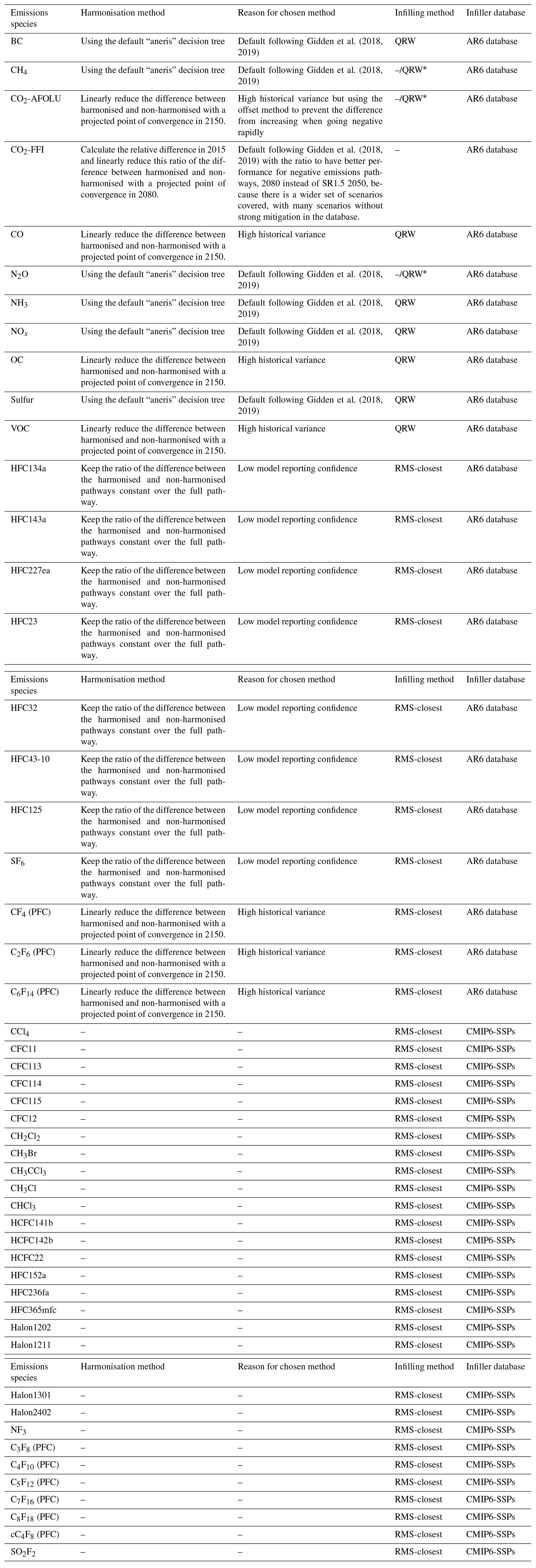
In principle, many methods to align modelled results with historical emissions could be used. In past IPCC assessments, ratio (multiplicative) methods (AR5) and offset (additive) methods (SR1.5) have been employed. Gidden et al. (2018) introduced a common approach for choosing which methods should be applied in different contexts (the so-called “default decision tree”). In AR6, this approach was used where suitable. For some species, however, a specific method was chosen in AR6. Table 1 provides an overview of the applied methods by emissions species, with more detail on all emissions and climate variable names as found in the AR6DB in Supplement Tables S3–S5. For CO₂-FFI, a ratio-based method was used with convergence in 2080, in line with the application of aneris for the CMIP6 process (Gidden et al., 2019). The convergence for 2080 is later than in SR1.5, which used 2050 (Forster et al., 2018). A later convergence year was seen as more suitable when considering scenarios across a wider range of mitigation futures than was considered in SR1.5. For CO₂ from AFOLU, an offset method with a convergence target in 2150 was used as the preferred method to deal with high historical interannual variability and large uncertainty in historical emissions estimates (Dhakal et al., 2022), leading to similarly large differences in historical emissions estimates from separate IAMs (IPCC, 2022d). All other emissions species with high historical variance are harmonised using a ratio method with a convergence target in 2150. Remaining F-gases are harmonised at the individual species level, increasing the detail compared with SR1.5, but because of low model reporting confidence a constant ratio harmonisation method is used. For all other emissions species, we use the default settings of Gidden et al. (2018, 2019).

Table 1 Harmonisation and infilling methods by emissions species as applied in AR6 WGIII. An asterisk (^*) means that the methods are in place but not used in the report because these emissions species were available for all 1202 assessed scenarios such that infilling was not necessary. The historical emissions database used for harmonisation was in all cases the database also used for RCMIP (Nicholls et al., 2021). Gidden et al. refers to Gidden et al. (2018, 2019). The reasons for varying the infilling method and database are explained in the text of this paper and are purely dependent on the availability of the number of modelled pathways and their independence in each database. QRW is used when a sufficient number of independent pathways is available in the AR6 infiller database (Kikstra et al., 2022b); otherwise, RMS-closest is chosen. CMIP6-SSPs is chosen as the database if the gas in question is not represented in the AR6 database.

For harmonisation, AR6 WGIII used the same historical emissions that were also used for the emissions-driven CMIP6 (Gidden et al., 2019) and Reduced Complexity Model Intercomparison Project (RCMIP) (Nicholls et al., 2020, 2021) emissions-driven runs. This data set is a combination of historical emissions databases. A significant share comes from the Community Emissions Data System (CEDS) database (Hoesly et al., 2018), but additional sources and methods have been used (for full details, see Nicholls et al., 2020, 2021, Gidden et al., 2019, and Kikstra et al., 2022a, c). The year 2015 was taken for harmonisation in line with CMIP6. In the case that IAM-reported values are not available for 2015 but were available for 2010 and 2020 emissions, the difference from historical data in 2010 was used to infer a 2015 value before harmonising. The benefit of using a similar data set and methods to those for emissions-driven CMIP6 and RCMIP, which informed the assessment by WGI, is that this leads to consistency between modelled temperature outcomes for emissions scenarios assessed by WGIII and the assessment of physical climate science by WGI and thus a stronger coherence across IPCC Working Groups within AR6.

3.3 Infilling of emissions pathways not reported by scenarios submitted to the AR6 database

If, for instance, a modelled scenario reports most climate-relevant species but not black and organic carbon, which are required by climate emulators to project temperature outcomes, the infilling process will supplement the model-reported results with an estimate of how black and organic carbon could develop along that modelled scenario. Infilling thus ensures that all climate-relevant anthropogenic emissions are included in each climate run for each scenario. This makes the climate assessment of alternative scenarios more comparable and reduces the risk of a biased climate assessment, because not all climatically active emissions species are reported by all IAMs. The infilling process in AR6 was performed using an open-source Python software package called “silicone” (Lamboll et al., 2020) integrated into the climate-assessment workflow (Kikstra et al., 2022a).

Different infilling methods result in different levels of proportionality, consistency, and stability to small changes. In AR6, the quantile rolling windows (“QRW”) approach was chosen for most reported emissions gases (aerosol precursor emissions, volatile organic compounds, and GHGs other than F-gases) because of the preference for high stability to small changes in the database. This is a conservative approach that cannot result in infilled pathways being more extreme than the database from which one infills (the “infiller database”). To avoid artefacts for the QRW method with a biased emissions space distribution in the infiller database, chlorinated and fluorinated gases are infilled based on a pathway with the lowest root-mean-squared difference (“RMS-closest”), ensuring a resulting emissions trend with consistency over time even when given few input emissions scenarios. See Table 1 and Supplement Tables S3–S5 for full details.

Where possible, missing emissions species are infilled from the harmonised AR6DB. Where the AR6DB does not cover the emissions species, the CMIP6-emissions SSP data set was used (Table 1).

Missing emissions pathways from a scenario are infilled based on their relationship with CO₂-FFI. If CO₂-FFI is strongly mitigated, the algorithm fills in pathways of other emissions species from other scenarios in the AR6DB where CO₂-FFI is mitigated similarly. This process is done based on emissions pathways that have already been harmonised. The AR6 WGIII report acknowledges that there is uncertainty in using this method and therefore chose to only use the climate results from scenarios where models natively provided at least CO₂-FFI, CO₂-AFOLU, CH₄, and N₂O. In principle, however, it would be possible to produce a climate assessment for a scenario that only reports CO₂-FFI, but while this would increase model diversity, such scenarios would still not be able to reflect the effect of policy choices that influence non-CO₂ emissions and hence climate outcomes from sectors such as AFOLU, waste, and industrial use of N₂O and F-gases.

3.4 Climate emulators

An extensive calibration and testing exercise of emulators to assess their suitability for reproducing assessed climate ranges has been undertaken in AR6 WG1 and reported in Cross-Chapter Box 7.1 of IPCC AR6 WGI (Forster et al., 2021; Smith et al., 2021a). The precedent for this exercise was RCMIP, where Phase 2 of this project compared emulators' performances when constrained to hit predetermined ranges of variables including equilibrium climate sensitivity (ECS), transient climate response (TCR), observed global mean surface temperature, ocean heat content change, transient climate response to cumulative emissions of carbon dioxide (TCRE), and radiative forcing for species such as CO₂, CH₄, and aerosols (Nicholls et al., 2021). One condition for an emulator to be used in the AR6 WGI emulator analysis was that the emulator needs to comprise an interactive carbon cycle and other gas cycle parameterisations so that it can run from emissions time series rather than from concentrations. In this exercise, emulators were driven by emissions time series of around 40 GHGs (with CO₂ broken down into CO₂-FFI and CO₂-AFOLU components), short-lived climate forcers, aerosol and ozone precursors, and external forcing from solar variability and volcanic stratospheric aerosol optical depth. Four emulators contributed to the AR6 WGI exercise: MAGICCv7.5.3, FaIRv1.6.2, CICERO-SCM, and OSCARv3.1.1. While we look at annual mean temperatures, these emulators do not aim to capture any unforced internal variability of the climate system.

MAGICCv7.5.3 and FaIRv1.6.2 were found to be able to reproduce Working Group I assessed climate variables to within a small error, with CICERO-SCM and OSCARv3.1.1 providing useful supporting information but with larger deviations from the temperature changes as assessed by WGI (Forster et al., 2021). Of these four, three (MAGICCv7.5.3, FaIRv1.6.2, and CICERO-SCM) connected to the workflow using the “openscm-runner” interface (Nicholls et al., 2022b) and participated in the AR6 WGIII process. The climate-assessment workflow provides 52 emissions species (see Table 1). Only information from MAGICCv7.5.3 and FaIRv1.6.2 was used in the Summary for Policymakers, and in the results section of this study we follow this focus on MAGICCv7.5.3 and FaIRv1.6.2, while we make some comparison with the climate outcomes from CICERO-SCM. The scenario classification and reported medians are based on MAGICCv7.5.3, while reported ranges were based on both MAGICCv7.5.3 and FaIRv1.6.2. As written in the WGI report, MAGICCv7.5.3 and FaIRv1.6.2 represent the WGI assessment typically to within ±5 % for central estimates of key climate change indicators, for instance for global warming in 1995–2014 compared with 1850–1900, warming estimates along SSPs in the 21st century, current ERF compared with 1750 ERF estimates, CO₂ airborne fractions under idealised experiments, and ocean heat content change between 1971 and 2018 (Forster et al., 2021, Cross-Chapter Box 7.1, Table 2). For the upper and lower ranges, the difference with the WGI assessment is within ±10 % across more than 80 % of the metric ranges (Forster et al., 2021). Despite some identified limitations like the lack of an interactive carbon cycle and projecting lower warming than the best assessment along SSPs (e.g. −14 % for SSP1–2.6 in 2081–2100 relative to 1995–2014), CICERO-SCM was assessed to represent historical warming very well and can be used for sensitivity analyses (Forster et al., 2021).

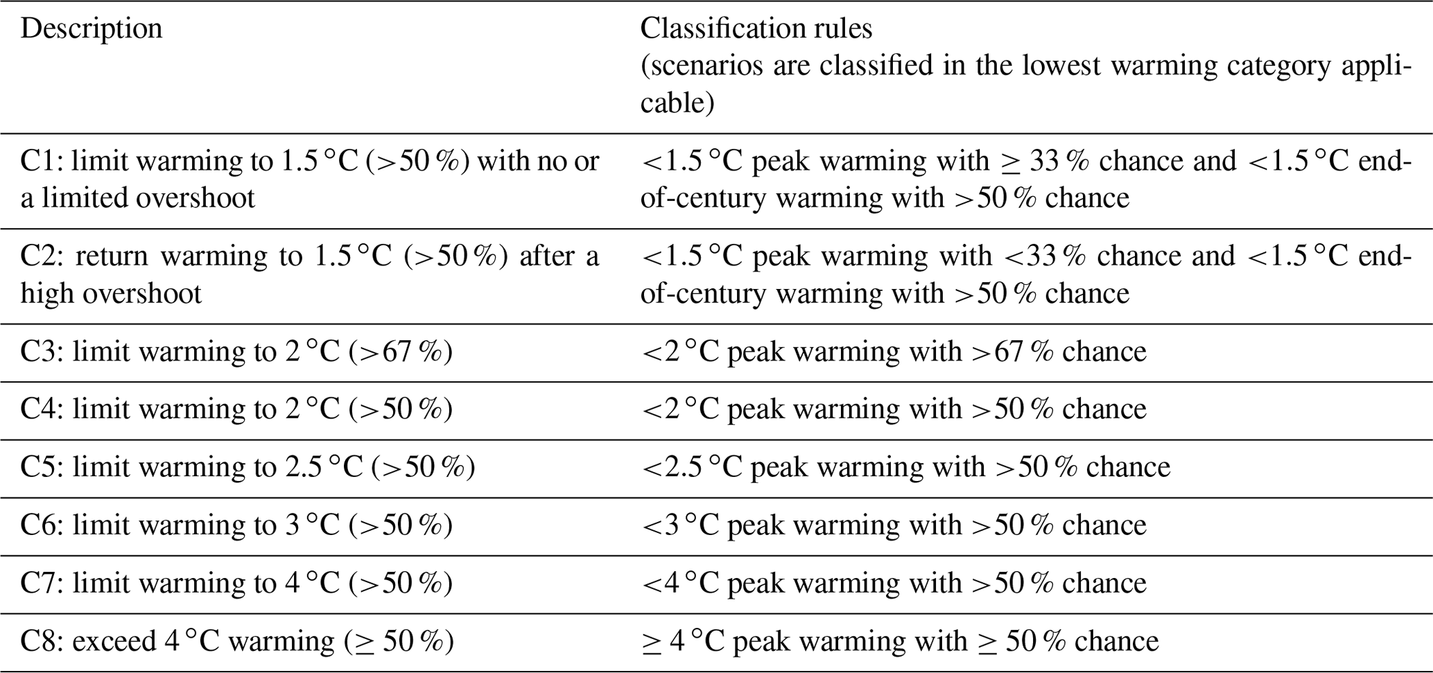
Table 2 Temperature classification rules used in AR6 WGIII, where a scenario is placed in the lowest category where it meets the classification rule.

3.4.1 MAGICC

MAGICC (Model for Assessment of Greenhouse gas Induced Climate Change) v7.5.3 is an emissions-driven Earth system model emulator. Its atmosphere is represented as four interconnected boxes (Northern Hemisphere and Southern Hemisphere ocean, Northern Hemisphere and Southern Hemisphere land). The ocean boxes are coupled to a 50-layer upwelling–diffusion–entrainment ocean model. A full description of MAGICC can be found in Meinshausen et al. (2011b), with updates as described in Meinshausen et al. (2020) and Nicholls et al. (2022a, 2021). MAGICCv7.5.3 was calibrated using the Monte Carlo Markov chain technique described in Meinshausen et al. (2009), with an updated step to re-weight the derived posterior to improve the match with the WGI-assessed ranges. The probabilistic distribution used in the climate assessment uses 600 ensemble members, balancing computational costs with ensemble size. As also described in the documentation of the climate-assessment workflow, the MAGICCv7.5.3 binary and probabilistic distributions are packaged separately from the climate-assessment workflow and can be accessed at https://magicc.org/download/magicc7 (last access: 15 December 2022) for use with the climate-assessment workflow.

3.4.2 FaIR

FaIRv1.6.2 is a fully open-source emissions-driven atmospheric model emulator with a state-dependent carbon cycle coupled to a two-ocean layer climate response module (Smith et al., 2018; Millar et al., 2017). The calibration for AR6 was performed using a 1-million-member prior ensemble. Parameters for the carbon cycle and climate response are derived from distributions based on CMIP6 models (Leach et al., 2021; Smith et al., 2018) and assessments made in AR6 WGI (Forster et al., 2021). This prior ensemble is simultaneously constrained on historical temperature (1850–2019), ocean heat content change (1971–2018), near-present-day (2014) CO₂ concentration, and airborne fraction of CO₂ in idealised 1 % per year CO₂ increase experiments at the time of doubled CO₂, the latter of which is assessed by Chapter 5 of WGI (Canadell et al., 2021). Post-constraint checks are performed to ensure that ECS, TCR, and future warming lie close to the AR6-assessed ranges. The constrained ensemble used for probabilistic assessment contains 2237 ensemble members. The calibrated, constrained ensemble for running FaIR is packaged separately from the climate-assessment package and is available as a JSON file from https://doi.org/10.5281/zenodo.5513021 (C. Smith, 2021).

3.4.3 CICERO-SCM

The CICERO simple climate model (CICERO-SCM, Skeie et al., 2017) is also an emissions-driven climate model emulator. The emulator consists of a carbon cycle model (Joos et al., 1996), simplified expressions relating emissions of components to forcing, either directly or via concentrations (Etminan et al., 2016; Skeie et al., 2017), and an energy balance/upwelling diffusion model (Schlesinger et al., 1992; Schlesinger and Jiang, 1990). The ensemble was based on a previously calibrated 30 400-member ensemble (Skeie et al., 2018). A 600-member subset of this ensemble was chosen to best fit the assessment made in WGI (Smith et al., 2021a), with a technique also described in Nicholls et al. (2021). For AR6 the ensemble was calibrated to the current temperature change from 1850–1900 to 1995–2014, with additional cut-offs for unrealistically low aerosol forcing or ECS values. The constrained ensemble for the climate assessment contains 600 members and is provided in a JSON file that is available with the climate-assessment workflow code (Kikstra et al., 2022a). CICERO-SCM has also recently been ported to Python, facilitating use on multiple computer operating systems.

3.5 Climate categorisation of scenarios

3.5.1 Scenario classification used in AR6

The extensive climate-assessment process provides increased confidence compared to previous assessments in the relationship between probabilistic temperature outcomes and the original modelled scenario. Therefore, the AR6 assessment used, like in SR1.5, a temperature-based set of classification rules, which are shown in Table 2. These categorisation criteria and their associated likelihoods are always associated with limits to global warming, looking at the simulated peak warming in the 21st century and the global mean surface temperature in 2100. For the categories that limit the global median temperature increase to less than 2 ^∘C above 1850–1900 levels (C1–C4), the categorisation rules follow the same scheme as in SR1.5. Beyond these, AR6 WGIII includes categories relevant for higher emissions scenarios that cover the 2–2.5 ^∘C (C5), 2.5–3 ^∘C (C6), 3–4 ^∘C (C7), and 4 ^∘C and higher (C8) global warming ranges, looking at modelled pathways until 2100. As already noted in SR1.5, temperature-based categorisation is affected by uncertainty in future warming, uncertainty in past warming, and the reference period against which temperature levels are compared (e.g. whether “pre-industrial”, which has a variety of interpretations, or specifically 1850–1900 is taken as a reference period; Chen et al., 2021), but the relative difference between warming levels and thus between temperature categories is more robust (IPCC, 2018).

3.5.2 Overshoot degree years

The categories C1 (“limit warming to 1.5 ^∘C (>50 %) with no or limited overshoot”) and C2 (“return warming to 1.5 ^∘C (>50 %) after a high overshoot”) are separated based on their level of overshoot of 1.5 ^∘C. This separation in the classification used in the IPCC report is purely based on the probability of overshoot (IPCC, 2022a), regardless of its magnitude or duration. In practice, however, the separation based on probability also corresponds to the peak temperature of overshoot. Here, we characterise this difference in overshoot for scenarios in more detail.

The extent and duration of the overshoot and the rate of change in overshoot temperatures are important for climate impacts (Hoegh-Guldberg et al., 2018). Temperature levels may be largely independent of the path dependence of CO₂ emissions and removals (Tokarska et al., 2019) under limited overshoot with limited permafrost feedbacks (Gasser et al., 2018), but many climate impacts are not (Seneviratne et al., 2018; Hoegh-Guldberg et al., 2018), including sea level rise and species extinction (IPCC, 2022b). For some impacts, the peak temperature during overshoot may be the most important factor, whereas in others it is rather the integral of overshoot (i.e. the magnitude of the overshoot combined with the duration of overshoot), such as sea level rise in 2300 (Mengel et al., 2018).

To further analyse the characteristics of scenario categories beyond the analysis in AR6, we use the concept of overshoot degree years (ODYs), which is similar to what was shown as “overshoot severity” in Table 2.SM.12 in SR1.5 (Forster et al., 2018) and was included in the metadata of the SR1.5 scenario database (Rogelj et al., 2018; Huppmann et al., 2018b) as “exceedance severity”. Inspired by Geden and Löschel (2017) and recent scenario studies investigating temperature overshoot (Drouet et al., 2021; Riahi et al., 2021; Johansson, 2021; Tachiiri et al., 2019), we add an analysis of the overshoot severity of all assessed pathways of the AR6 WGIII report as the cumulative years above a certain global warming level, multiplied by the projected average annual climatic ^∘C overshoot in each year.

In this study, we look at ODY_1.5 (^∘C ⋅ year) as the cumulative overshoot degree years above 1.5 ^∘C relative to 1850–1900 from the start of each scenario until 2100 or the year specified otherwise: ${\sum }_t\max (\mathrm{0},T_t-T_{\mathit{\theta }})$, where T is the annual mean climatic global warming above 1850–1900, t is the year, and T_θ is the overshoot threshold temperature. The indicator could allow one to define limits for overshoot targets and thus be related to net-negative emissions in scenarios that return to below 1.5 ^∘C. Additionally, it could be useful in studies that investigate the irreversibility of certain climate change impacts and could be an indicator of the resilience of a system. For instance, in the case that some human system or ecosystem is unable to adapt permanently but would be able to withstand up to 10 ODY_1.5, either through limited resilience or by using temporary adaptation measures, this would indicate when, under a certain scenario, the system may collapse. The AR6 Working Group II (WGII) report on Impacts, Adaptation and Vulnerability (IPCC, 2022b) states with medium confidence that shorter durations and lower levels of overshoot are projected to come with less severe impacts. ODY is not an indicator that can be used for all purposes, as for some questions the rate of temperature change or the level of peak warming reached in a given scenario may be more relevant. Still, at the very least an indicator like this acknowledges that not only the magnitude of overshoot, but also the timescales, are important when assessing overshoot risks (Ritchie et al., 2021) and bridges the gap with stylised overshoot scenarios (Huntingford et al., 2017). Analysing IAM scenarios in this way could be a useful link to the broader tipping point literature (Lenton et al., 2019) and potentially inform climate change policy, impact, and adaptation studies.

3.5.3 Alternative policy-relevant scenario classifications

There are multiple possible indicators that can be chosen to classify and group scenarios (see the discussion above and e.g. Table 3.4 in AR4 WGIII; IPCC, 2007). AR4 discussed this mainly as a matter of stabilisation of greenhouse gas concentrations using a specific indicator as a proxy along the chain from mitigation costs through emissions to impacts. In response to the introduction of temperature goals in international policy decisions and the spearheading of a temperature-aligned approach in science-policy reports by the UN Environment Programme (Hare et al., 2010; Rogelj and Shukla, 2012; Rogelj et al., 2011), SR1.5 and AR6 WGIII based their classifications on global warming levels. Global warming levels were used as one of the integrating dimensions in the AR6 WGI report (Chen et al., 2021) and in the AR6 WGII report as well as across WGs. However, it is also possible to append such a classification with a mix of indicators, for instance to reflect a global climate agreement like the Paris Agreement. For example, the IPCC WGIII AR6 report also reports a sub-category, C1a, of C1 scenarios (IPCC, 2022d). The additional criterion for this sub-category is that net-zero GHG emissions are attained, generally in the second half of this century, which can be interpreted to reflect Article 4.1 of the Paris Agreement (Fuglestvedt et al., 2018; Rogelj et al., 2021). Related examples of such mixed classifications exist in the literature. For example, one recent paper proposes a specific interpretation of the Paris Agreement (Schleussner et al., 2022), proposing that pathways can be seen as “Paris-compatible” if they (a) “[do] not ever have a greater than 66 % probability to overshoot 1.5 ^∘C”, (b) “[are] very likely (90 % chance or more) … not ever exceeding 2 ^∘C”, and (c) achieve net-zero greenhouse gas emissions using global warming potentials with a 100-year time horizon (GWP100).

3.6 Evaluating the effects of each step of the climate-assessment workflow

The approach to emissions processing in AR6 WGIII was based on a combination of the previous literature (Lamboll et al., 2020; Gidden et al., 2018) and expert evaluation of the submitted pathways. The objective of this approach is to obtain an unbiased, comparable, and plausible set of climate outcomes, in which each climate time-series outcome reflects the original pathway as truthfully as possible. To facilitate expanding and improving the methods, it is worth evaluating the appropriateness of the set of tools in a quantitative manner. In this work, we provide an initial analysis by showing the effect on the total Kyoto gases using a CO₂-equivalent emissions indicator (based on GWP100) for both harmonisation and infilling for each category.

4 Results

4.1 Characteristics of the full database

The 1202 scenarios for which a climate assessment is available in the AR6DB span a wide range of emissions pathways (Fig. 2a). The three climate emulators CICERO-SCM, FaIR, and MAGICC translate the set of infilled pathways in similar ways for atmospheric concentrations, with most distinctive differences for N₂O (Fig. 2b). Global mean surface temperatures above 1850–1900 levels are relatively similar between MAGICC and FaIR, while CICERO is colder (Fig. 2c). Global mean surface temperature change in IPCC WGIII AR6 (and here) is defined as degrees Celsius above the 1850–1900 mean, normalised to the best estimate of 0.85 ^∘C global warming for the period 1995–2014, as given by AR6 WGI.

In this paper, we focus on the median simulated climate outcomes of each scenario, with percentiles generally indicating percentiles over the selected scenario set. However, each climate variable, also including variables not discussed in this article such as ERF, ocean heat uptake, and CO₂ and CH₄ fluxes as well as non-CO₂ warming for MAGICCv7.5.3, is available for each scenario for percentiles 5, 10, 16.7, 25, 33, 50, 67, 75, 83.3, 90, and 95 (Byers et al., 2022). The full AR6DB thus enables rich future studies of the uncertainty in multiple climate indicators for a large scenario set.

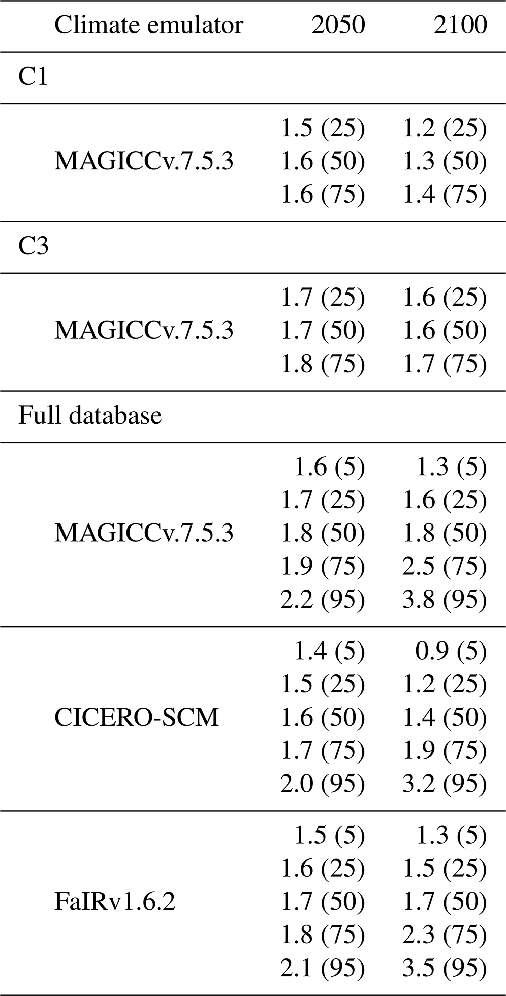
The database has scenarios (across all categories C1 to C8) with a very wide range for 2100 temperature outcomes, with its 5th to 95th percentile range stretching from 0.9–1.3 to 3.2–3.8 ^∘C across scenarios, with the range for both the 5th and 95th percentiles arising from the differences across the three climate emulators. In 2050, the temperature outcome range is much smaller, covering a range of 1.4–1.6 to 2.0–2.2 ^∘C above 1850–1900 (Table 3). The database thus covers a very broad spectrum of scenarios, going from groups of scenarios that reduce emissions quickly enough to let temperatures decline in the second half of the century to scenarios that project increasingly fast warming. Still, it is noteworthy that the extreme ends of the range are covered by only a few scenarios, with scenarios reaching 4 ^∘C warming this century reflecting less than 5 % of the scenarios in the AR6DB and only very few scenarios in the database that stay below 1.5 ^∘C by mid-century (except for when assessed using CICERO-SCM, which is cooler and features a larger set of scenarios staying below 1.5 ^∘C, and was used as a sensitivity case in the AR6 WGIII full report but was not included in the summary of results reported in the Summary for Policymakers).

Table 3 Median global temperature statistics of the full scenario database, by climate model, with the percentiles over the scenarios in parentheses for each row.

4.2 Differences in climate emulators

The temperature classification in IPCC AR6 WGIII was done based on MAGICC. In high-emissions scenarios MAGICC generally projects higher median outcomes than the other two emulators for the same set of scenarios (Fig. 3a). The CICERO AR6-calibrated version projects the lowest amount of warming of the three emulators for all scenario categories.

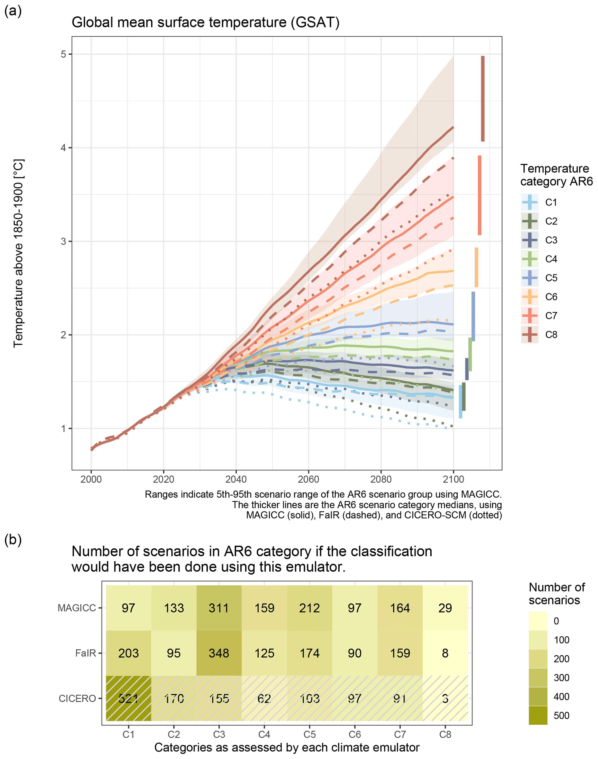
Figure 3 Median global surface temperatures above the mean of 1850–1900 as simulated for scenarios in the AR6DB, with scenarios grouped by the classification as in AR6 WGIII. Medians are shown for all three uses of climate emulators (CICERO-SCM: dotted, MAGICCv7.5.3: solid, and FaIRv1.6.2: dashed), while the 5th–95th percentile range is only shown for MAGICCv7.5.3. The number of scenarios classified in each group are shown in the bottom panel. CICERO-SCM numbers are hashed to indicate that AR6 WGI assessed especially the used parameterisations of MAGICCv7.5.3 and FaIRv1.6.2 to closely reflect the IPCC assessment, with CICERO-SCM for its AR6 calibration being used in WGIII only for sensitivity analysis to capture climatic uncertainty ranges.

For the two scenario categories with the most stringent temperature limits (C1 and C2), the medians of MAGICC and FaIR in 2100 are very close to each other. However, for these two categories MAGICC projects faster near-term warming than FaIR for the same emissions, and thus MAGICC projects higher peak temperatures. Together, this implies a more negative zero emissions commitment (ZEC) in MAGICC compared to FaIR.

One way to investigate the difference in climate emulators is to look at the same scenario set and compare the relative contributions of different emissions species to warming using median ERF. Looking at the ERF across scenarios for the AR6DB split up into lower (C1–C4) and higher (C5–C8) temperature categories, it is clear that MAGICC and FaIR perform very similarly, with slightly stronger negative aerosol forcing in MAGICC and slightly stronger positive CO₂ forcing in FaIR (Fig. 4a). CICERO shows clearly lower CO₂ forcing than the other two emulators while also having less negative aerosol forcing.

Figure 4 (a) Effective radiative forcing (ERF) statistics across AR6 scenario database subsets as categorised by AR6WGIII using MAGICC for CO₂, CH₄, F-gases, and aerosols at different points in time for three climate emulators. (b) Climate uncertainty for every scenario as represented in projected ERF in 2030 for each climate emulator, with a range representing the 5th to 95th percentile range across scenarios. For aerosols this uncertainty in forcing is still relatively unconstrained and depends heavily on the magnitude and mix of emissions within a scenario.

Looking not at the ranges across scenarios, but rather at the climate uncertainties for each scenario in 2030, we see that the uncertainty ranges projected by FaIR and MAGICC are also similar, though MAGICC projects somewhat higher uncertainty ranges on near-term forcing from F-gases and aerosols (Fig. 4b). CICERO does not have an interactive carbon cycle representation and only represents uncertainties in aerosols, which are much smaller than in MAGICC and FaIR, where uncertainty in aerosol-related ERF is especially large.

4.3 Characteristics of scenario categories

A multi-emulator comparison reveals that the temperature categorisation of a specific scenario can be quite sensitive to small differences in how emissions are translated to global warming (Fig. 3b). This is especially the case for the C1 and C2 categories, with many scenarios in the AR6DB aiming at 1.5 ^∘C targets, while warming is already 1.1 ^∘C for the period of 2011–2020 over 1850–1900 (IPCC, 2021a). FaIR and MAGICC were assessed to cover the AR6 WGI assessment and its uncertainties very well, which can be interpreted as generally approximating best estimate warming with an error of up to 0.1 ^∘C difference. While small in the broader context of uncertainty in the physical climate system, a 0.1 ^∘C difference in projected peak temperature covers a non-trivial part of the difference between C1 and C2. Since FaIR projects slightly lower peak temperatures than MAGICC, the number of scenarios classified in the AR6 temperature category C1 would double if the classification would be repeated using FaIR. However, the number of scenarios in the wider set of 1.5 and 2 ^∘C consistent categories (C1–C4) is much more similar, with 758 for FaIR versus 687 for MAGICC.

In the Supplement, we perform sensitivity experiments to explore the sensitivity to changes in absolute warming level estimates of the number of scenarios within temperature categories C1–C3 (Supplement Fig. S1). Such changes could happen for instance due to a change in the best estimate of historical warming since 1850–1900, an update of the best estimate of CO₂ or aerosol forcing, or even choosing different harmonisation and infilling methods. If the peak temperature estimates of all scenarios had been 0.1 ^∘C higher, virtually no scenarios would be categorised as C1, while the number would roughly double if peak temperature level estimates were about 0.1 ^∘C lower (Supplement Fig. S1a–b). Furthermore, small variations in the scenarios included in a category can have a marked impact on the median net-zero GHG timing in C1, while the effects on net-zero CO₂ in all categories and on net-zero GHG in C2 and C3 are less sensitive (Supplement Fig. S1c–d). This simple sensitivity analysis of the level of global temperatures gives a sense of how much scenario categorisation is related to uncertainty in climate projections of emissions pathways. This can be connected to the change in categorisation that may come with a potential change in harmonisation and infilling methods, but it is not immediately obvious what effect a change in harmonisation or infilling would have on categorisation. In Sect. 4.7 of this article, we discuss the temperature change that can be attributed to changes in climate-assessment methods between SR1.5 and AR6, providing an initial analysis by showing the magnitude of the changes between the two applications. However, a full analysis of the uncertainties in the climate-assessment workflow is beyond the scope of this paper and remains a topic for further research.

4.4 Temperature overshoot

Almost all scenarios are projected by MAGICC to overshoot 1.5 ^∘C, even in C1, with C3–C8 median warming estimates never returning to below 1.5 ^∘C this century (Fig. 5a–d). The duration of overshoot in most C1 scenarios is limited to a few decades, generally starting in the 2030s, while some C2 scenarios are projected to have a global warming of more than 1.5 ^∘C for most of the century (Fig. 5b–c). The peak of overshoot in C1 scenarios is generally limited to up to 0.1 ^∘C, while scenarios in C2 are generally in the 0.1–0.4 ^∘C range. Hence, even though categories C1 and C2 are defined solely based on their probability of exceeding 1.5 ^∘C, these scenarios are also practically distinguished by the amount by which they overshoot 1.5 ^∘C, which may be more relevant for climate change impact, vulnerability, and adaptation studies. Notably, there is some overlap in ODY1.5 between categories. For instance, there are scenarios in the C2 and C3 categories that have lower ODY_1.5 than a number of scenarios in C1.

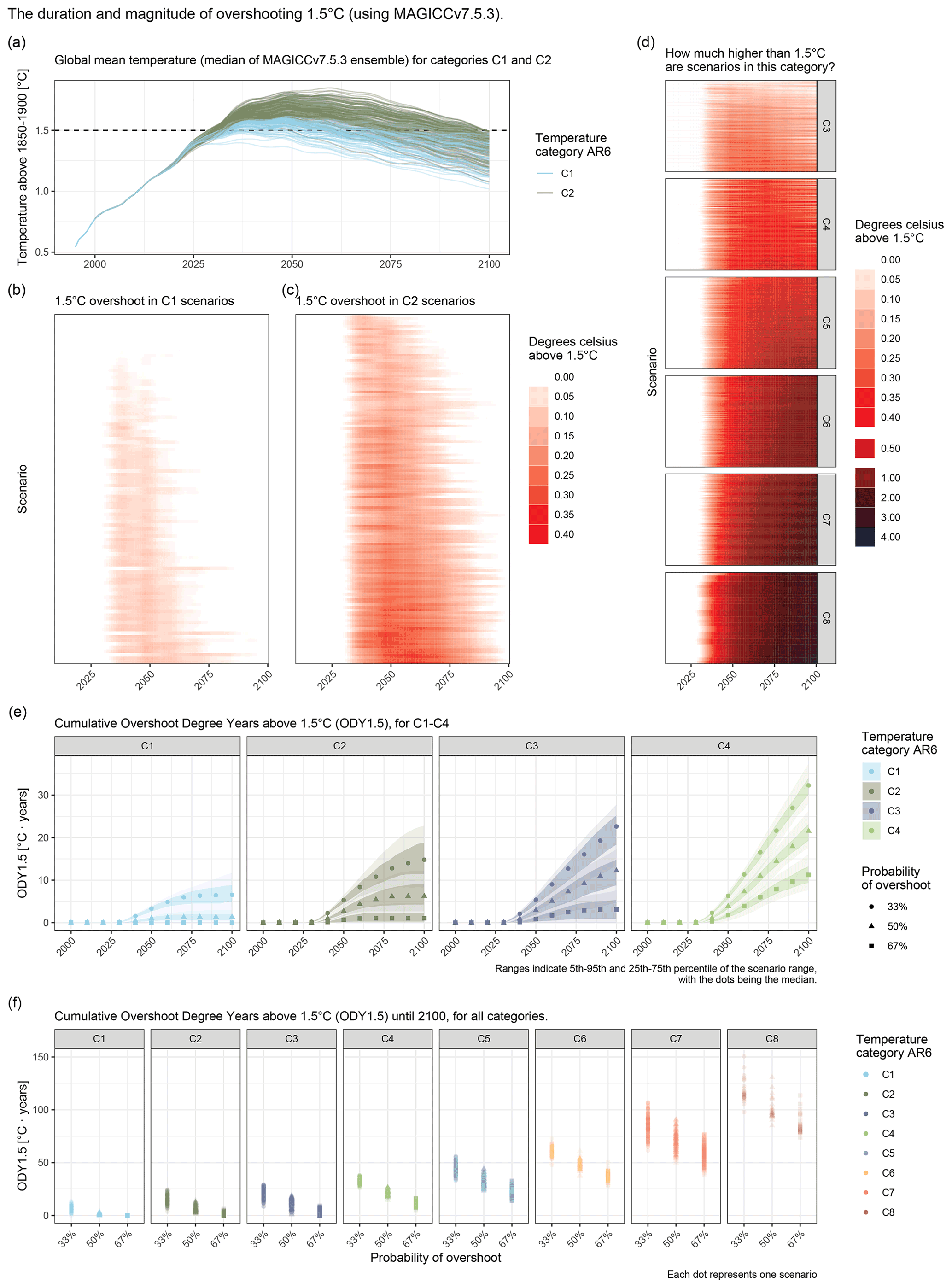
Figure 5 The duration and magnitude of overshoot and exceedance of 1.5 ^∘C global warming above 1850–1900 for scenarios in the AR6 temperature categories. Panel (a): projected median global mean surface temperature for scenarios in C1 and C2. Panel (b)–(c): magnitude and duration of the overshoot of 1.5 ^∘C in the C1 and C2 scenarios. Panel (d): magnitude of 1.5 ^∘C exceedance of scenarios in C3–C8. For panel (b)–(d), scenarios along the y axis are sorted by total ODY_1.5 until 2100. Panel (e): projected increase in ODY_1.5 over time for temperature categories C1–C4 at 33 %, 50 %, and 67 % probabilities. Panel (f): projected cumulative exceedance of 1.5 ^∘C expressed as ODY_1.5 in 2100 for temperature categories C1–C8 at 33 %, 50 %, and 67 % probabilities.

Using ODY_1.5 until 2100, we see that the severity of temperature exceedance above 1.5 ^∘C is also clearly differentiated by category, with different rates of increase in cumulative exceedance of 1.5 ^∘C after 2030 (Fig. 5e–f). For instance, using the median of temperature estimates from MAGICC, we find that about three-quarters of the scenarios in C1 stay below 2 ODY_1.5, and the 95th percentile across scenarios is slightly below 3 ODY_1.5 (Fig. 5e). If the warming response is on the higher end of the spectrum, at 33 % probability (67th percentile of the warming range), the ODY_1.5 interquartile (25th to 75th) scenario range is about 5 to 9, meaning a risk of significant overshoot even for C1. Only if the warming response would be on the lower end of the spectrum (67 % probability at the 33rd percentile of the warming range) could overshoot be avoided for all C1 scenarios. C4 scenarios are more likely than not below 2 ^∘C but do not return back to below 1.5 ^∘C. Their median ODY therefore steadily grows to over 20 ODY_1.5 by the end of the century for more than half of the scenarios. For more than half of the scenarios in C4, more than 10 ODY_1.5 by 2100 is projected with at least 67 % chance and about 33 % chance that it would be more than 30 ODY_1.5. In higher temperature categories, ODY_1.5 increases ever more quickly over time because temperatures keep increasing, resulting in median values of about 50 and 100 ODY_1.5 in 2100 for C6 and C8 in 2100, respectively (Fig. 5f).

4.5 “Paris-compatible” scenarios using FaIR and MAGICC

Using FaIR, 89 scenarios in the AR6DB would meet the three criteria for “Paris-compatibility” from Schleussner et al. (2022) described in Sect. 3.5.3. Using MAGICC, 29 scenarios meet these criteria (Fig. 6a). In this subset of scenarios, net-zero CO₂ in the MAGICC scenario subset is reached around 2050 and before 2060 in the FaIR subset, looking at the interquartile range, with the median of both subsets being close to 2050. Net-zero GHG timing has a wider range across scenarios, with the medians across scenario subsets being about 15–20 years later than net-zero CO₂ (Fig. 6b). Compared with the “Paris-compatible” set, the IPCC C1 category has a much wider range for GHG net-zero timing, with a few scenarios that do not have net-negative GHG emissions but do have projected warming of less than 1.5 ^∘C in 2100. For net-zero CO₂ timing, the difference is small. The interquartile ranges for cumulative CO₂ emissions until net-zero CO₂ are 520–680 Gt CO₂ for FaIR and 480–560 Gt CO₂ for MAGICC. How remaining carbon budgets relate to temperature outcomes is strongly dependent on the level of non-CO₂ mitigation (Canadell et al., 2021; Riahi et al., 2022; IPCC, 2022a). However, even with the strongest non-CO₂ mitigation, no scenario with more than 1000 Gt CO₂ cumulative emissions before reaching net zero is deemed Paris-compatible according to these criteria using FaIR, or no more than 800 Gt CO₂ using MAGICC.

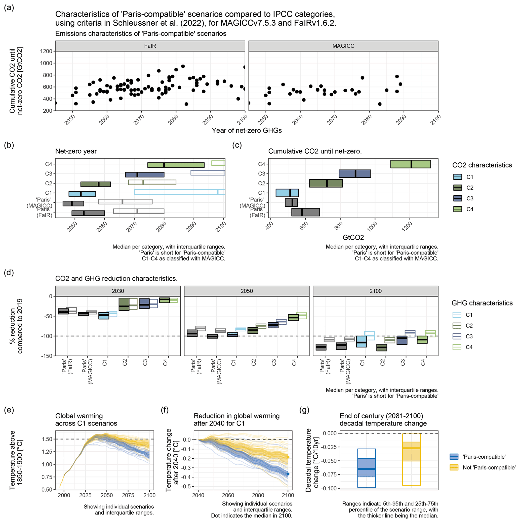
Figure 6 Characteristics of “Paris-compatible” scenarios using the FaIR and MAGICC emulators compared to the C1–C4 categories from IPCC AR6 WGIII, which used the MAGICC emulator for classification. “Paris” here is short for “Paris-compatible” and uses the criteria from Schleussner et al. (2022), being (a) “not ever having a greater than 66 % probability of overshooting 1.5 ^∘C”, (b) “very likely (90 % chance or more) […] not ever exceeding 2 ^∘C”, and (c) achieving net-zero greenhouse gas emissions using global warming potentials over a 100-year period (GWP100). Panels (e)–(f) are based only on MAGICC.

The main climate difference between the “Paris-compatible” scenarios and the full C1 category is the amount by which temperature declines after its peak at 1.5–1.6 ^∘C in 2035–2055 (Fig. 6e). For more than half of the scenarios in the sub-group of 29 scenarios the temperature decline after 2040 is 0.3–0.4 ^∘C until 2100, whereas more than half of the other C1 scenarios see less than 0.2 ^∘C temperature decline post-2040 in this century (Fig. 6f). The temperature decline in the “Paris-compatible” (∼ 0.06 ^∘C per decade) subset is about 2 times faster than the C1 subset that is not “Paris-compatible” (∼ 0.03 ^∘C per decade, Fig. 6g). Such lower temperatures, which are also implied to decline beyond 2100 if no abrupt changes in emissions levels and trends are assumed, come with lower risks related to, for instance, sea level rise and stresses related to heat extremes and drought, given that temperatures would return towards current levels during the 22nd century. Conversely, some scenarios that are in C1 but not classified as “Paris-compatible” are characterised by even stronger CO₂ reductions by 2030 than the already very rapid reductions in the “Paris-compatible” set. Those scenarios thus project even more rapid near-term reduction to limit warming while avoiding reducing the need for net-negative CO₂ emissions present in the second half of the century in scenarios that reach net-zero GHG emissions, as illustrated by Fig. 6d.

4.6 The effects of emissions processing in the AR6 workflow

The effects of harmonisation and infilling on input emissions pathways are small when taken over the entire scenario database, looking at GHGs for Kyoto gases using GWP100 to calculate CO₂-equivalent values for N₂O, CH₄, and F-gases. The median effect of harmonisation and infilling over the full scenario database is about 1 Gt CO₂ eq. yr⁻¹ upwards in 2015, trending down to zero towards the end of the scenario in 2100 (Fig. 7a). However, some scenarios are affected by these processing steps much more than others, with the 5th to 95th percentile range of about −2 to 4 Gt CO₂ eq. yr⁻¹ in 2020 (compared to total modelled emissions of around 55 Gt CO₂ eq. yr⁻¹ in 2020) to −1 to 4 Gt CO₂ eq. yr⁻¹ in 2100. Investigating in which scenarios such changes occur, and for which emissions species, helps understand differences with other harmonisation and infilling methods as discussed in the next section.

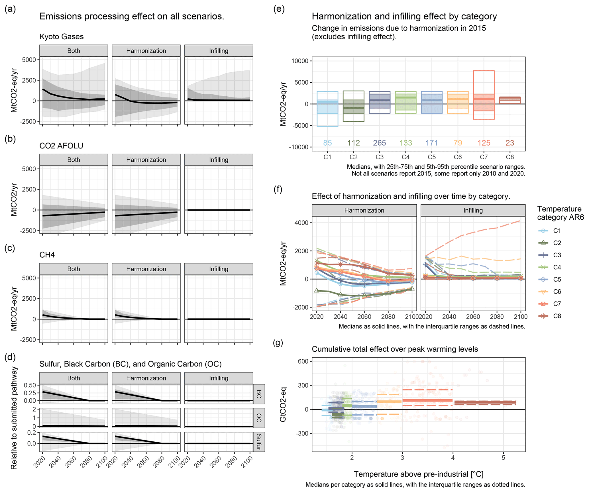
Figure 7 Effect of harmonisation and infilling processing steps on Kyoto gas emissions trajectories. Panel (a)–(c): the effect of harmonisation and infilling over time on GHGs (Kyoto gases), CO₂-AFOLU, and CH₄ for the full AR6DB. Panel (d): the relative effect of harmonisation and infilling over time on BC, OC, and sulfur emissions for the full AR6DB. Panel (e)–(f): effects of emissions processing by AR6 temperature category. Panel (e): the effect on GHGs in 2015 due to harmonisation. Panel (f): the effect of harmonisation and infilling on GHGs over time. Panel (g): the cumulative effect of emissions processing until 2100 over the projected global warming.

While the harmonisation effect decreases over time, the upper bound does not change much because it is dominated by infilling effects in the second half of the century. Such a high infilling is almost always the result of high-emissions scenarios lacking detail in reporting F-gases, which can grow to more than 5 Gt CO₂ eq. yr⁻¹ in 2100 in a set of high-emissions scenarios. As shown in Fig. 7a–c, about half of the total effect on the outer ranges is due to the harmonisation of CO₂-AFOLU, for which a large model spread exists, much in line with the uncertainty in historical databases (Dhakal et al., 2022). For methane, and for all other long-lived greenhouse gases combined (N₂O and F-gases), the median of harmonisation is slightly positive. Most scenarios require little to no infilling for Kyoto GHGs measured in CO₂ equivalence, but that does not mean that they are unaffected by infilling as they may still need significant infilling for aerosols and precursor emissions. We do not find evidence that harmonisation and infilling introduce any particularly strong bias across the climate categories used in the IPCC AR6 WGIII report (Fig. 7e–f). For harmonisation, for each category except C8 (which has the smallest number of scenarios), the zero line falls well within the interquartile range, with the C2 median being most negative, and the C4 median being the most positive (Fig. 7e). In terms of infilling, only the C3 and C7 median effect across scenarios show values larger than 0.3 Gt CO₂ eq. yr⁻¹ due to infilling before 2040 (Fig. 7f). The emissions processing also affects climate forcers beyond the Kyoto gases, which are not readily expressed in GWP100 CO₂-equivalent values. Most evaluated scenarios model non-Kyoto climate forcers such as BC, organic carbon (OC) and sulfur, and thus there is no infilling effect for most scenarios for these emissions species. However, the relative difference in reported past emissions can be quite large leading to a harmonisation effect, with a small fraction of outliers for OC (Fig. 7d).

The total cumulative effect of infilling and harmonisation for the 2020–2100 period is relatively small too (Figs. 7g and 8). More than half of the scenarios in the AR6DB (738) have higher cumulative Kyoto gas emissions until 2100 after harmonisation and infilling, and 464 scenarios are lower, indicating that the infilling effect is not dominating the harmonisation effect. In part, the infilling effect is offset due to a large number of scenarios which report CO₂-AFOLU emissions levels higher than the ∼ 3.5 Gt CO₂ yr⁻¹ harmonised value in 2015, in combination with the late convergence target year for CO₂-AFOLU. Virtually all scenarios fall well within the ±500 Gt CO₂-equivalent band (Fig. 8b), with the majority of scenarios being affected less than the 100 Gt CO₂ equivalent. All except eight of the C1–C5 scenarios fall within the ±250 Gt CO₂-equivalent band (Fig. 8a). Thus, this analysis does not show a clear pattern or bias pushing emissions up or down across categories. Rather, the harmonisation and infilling effect is mostly model-dependent, and the distribution of scenarios from certain IAM frameworks is not constant across temperature categories (Supplement Table S2).

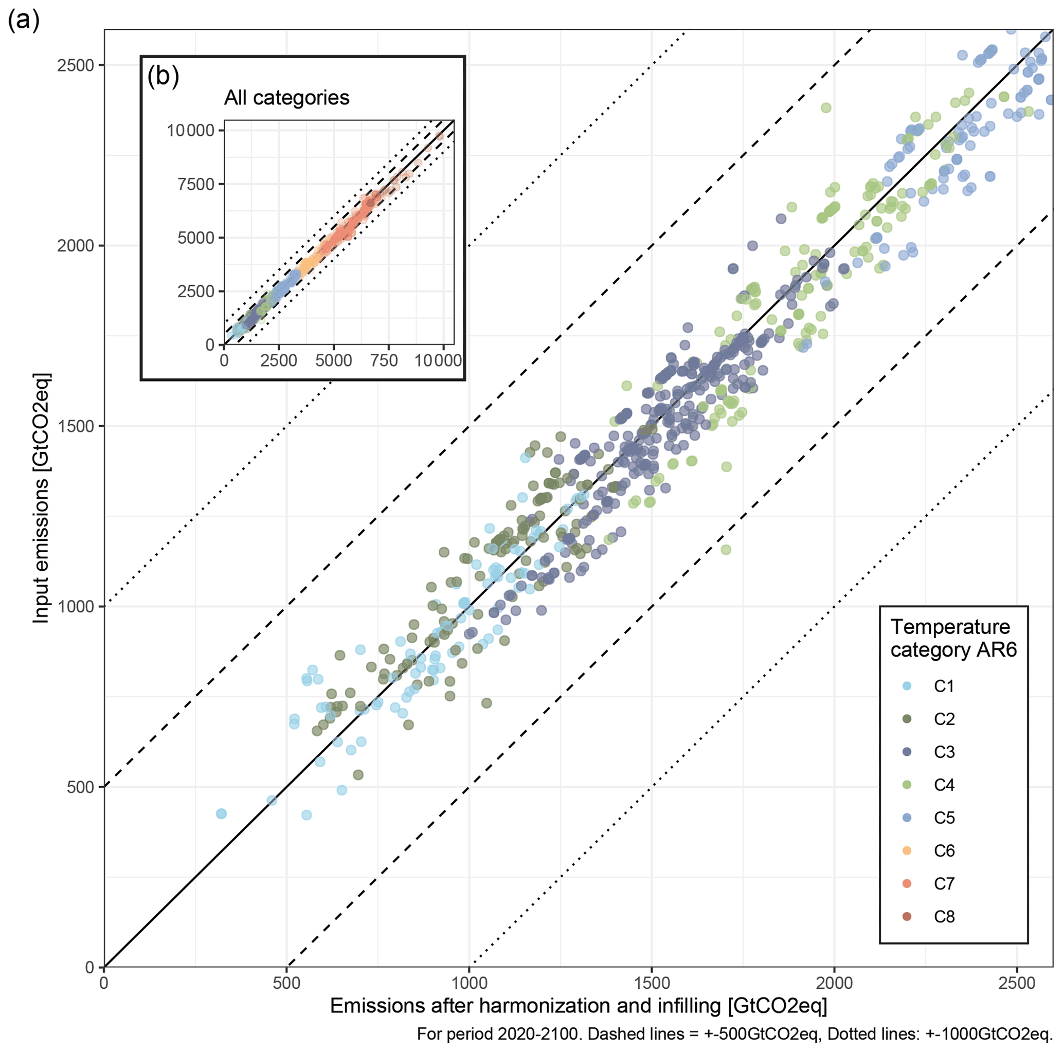
Figure 8 Kyoto gases for 2020–2100, infilled and model reported by category. Each dot represents one long-term full-century scenario. If model input would perfectly align with the used historical database and model all emissions species or if harmonisation and infilling cancel each other exactly, the input GHG emissions would be the same as the GHG emissions after harmonisation and infilling. A spread on both sides of the line would be expected if historical emissions uncertainty would dominate, and the use of different modelled historical emissions would not have a particular bias compared to the emissions estimate used for harmonisation. On the other hand, if many scenarios miss information on some important GHGs, dots would appear predominantly on the right of the line.

4.7 Changes in methods between SR1.5 and AR6 WGIII and their implications

The most recent and most rigorous scenario assessment until AR6 was done in SR1.5. Insights from IAM-based assessment have influenced the global science-policy discourse (van Beek et al., 2020, 2022) and are even referred to in outcomes from informed ambitions in the Glasgow Climate Pact (UNFCCC, 2021). The results of SR1.5 have been influential in the academic literature, influenced public debate around the world, and legitimised as well as challenged climate policy (Hermansen et al., 2021; Livingston and Rummukainen, 2020). It is thus crucial to understand how the AR6 assessment methods differ from the methods applied in SR1.5. Here we provide additional insights to Annex III.II.3.2.1, “Climate classification of global pathways”, of AR6 WGIII (IPCC, 2022a). The analysis performed allows for isolating the approximate differences between SR1.5 and AR6 WGIII pertaining to each of the separate methodological steps of the climate-assessment workflow, namely harmonisation, infilling, and climate emulation. The same set of emissions scenarios was run with five different configurations that are summarised in Table 4.

Table 4 Summary of five climate-assessment runs done to isolate the approximate changes in the temperature outcome attributable to each step of the climate-assessment workflow.

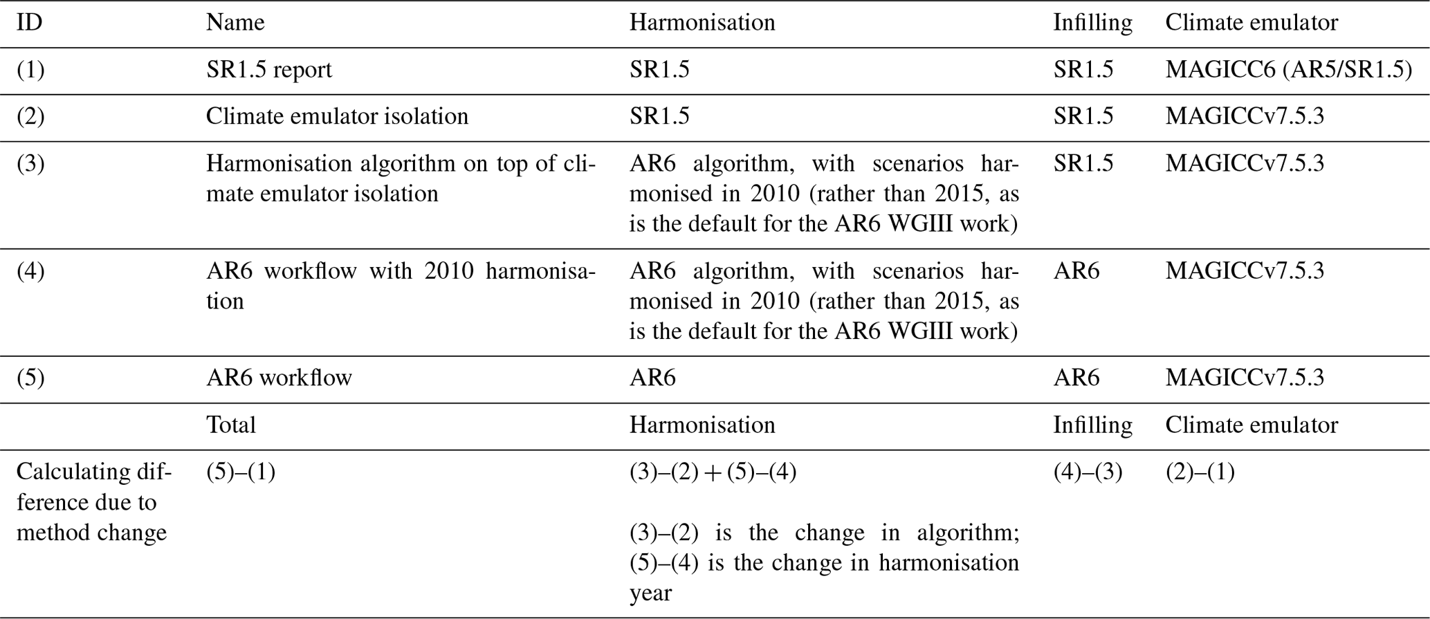
Analysing the scenarios available in both the AR6 database as well as the SR1.5 database (see also IPCC, 2022a), using the climate emulator MAGICC shows the effect that is due to partly compounding, partly offsetting changes in each stage of the climate assessment (Fig. 9a and b).

Figure 9 Differences in the AR6 and SR15 climate-assessment workflow steps (a and b) and the temperature outcome distributions (c) using MAGICC. In panels (a) and (b), the AR6 temperature categories for a specific scenario were used. In panel (c), we use the categories as reported in the separate IPCC reports. SR1.5 categories “1.5C low overshoot” and “Below 1.5C” have been mapped as C1, “1.5C high overshoot” as C2, “Lower 2C” as C3, and “Higher 2C” as C4.

The effect of the climate emulator update and recalibration (MAGICC6 in SR1.5 versus MAGICCv7.5.3 in AR6 WGIII) means a slightly higher peak temperature for near-term temperature peaks (in C1 and C2) and a lower 2100 temperature for all scenario categories in AR6. The lower warming in 2100 in AR6 is more in line with the best estimate based on multiple lines of evidence in AR6 WGI, as expressed by a lower transient climate response in MAGICCv7.5.3 (Nicholls et al., 2022a).

The median harmonisation effect for C1 and C3 results in about 0.05 ^∘C lower temperature in the AR6 method, which may in part be explained by the difference in harmonisation year (2010 in SR1.5 versus 2015 in AR6 WGIII) as well as a later chosen convergence date for CO₂-AFOLU. However, an explicit analysis of these separate factors is beyond the scope of this paper.

The change in infilling methods results in slightly lower 2100 temperatures in AR6 for C1 but virtually zero for C3 and positive ones for high warming categories (particularly C7 and C8). This is not surprising because in SR1.5 infilling was done using RCP2.6, which is roughly consistent with C3. Scenarios in C1 see stronger mitigation, and thus the infilling method applied in AR6 WGIII also sees more strongly declining emissions from other GHGs that are being infilled.

Overall, the effect of updating climate-assessment methods is typically less than 0.2 ^∘C and for most scenarios less than 0.1 ^∘C (Fig. 9a). This difference is small but non-negligible compared to the precision of the climate emulators. If we only look at the projected warming since 1995–2014 (which was calibrated to 0.85 ^∘C above the pre-industrial), the effect of the change in methods is always less than 25 % of the projected warming in each scenario and typically less than 10 % for both peak temperatures and 2100 temperatures (Fig. 9b). Only for the C1 and C2 categories is the change in 2100 more substantial when expressed as a percentage of recent and future warming; this is due to the limited warming that occurs overall in this category, so that even small changes result in a more substantive percentage change of about 30 % in the median of C1. This, however, still only corresponds to an absolute median temperature difference of about 0.1 ^∘C.

There are a few outlier scenarios in C1 and C2, where the relative effect on projected warming in 2100 relative to 1995–2014 is more than 50 %. These differences, both when negative and positive (up to ±0.2 ^∘C change), are mostly caused by a different infilling effect for scenarios that have a low projected warming until 2100, sometimes combined with a slightly more negative temperature drawdown after peak from the climate emulator. The effects are strongly scenario-dependent. For instance, the change in 2100-projected temperature due to changes in infilling is opposite for the AIM/CGE (AR6 infilling results in higher temperatures than SR1.5 infilling) and WITCH-GLOBIOM CD-LINKS_NPi2020_400 (AR6 infilling results in lower temperatures than SR1.5 infilling) scenarios.

Lastly, to understand the differences in reported summary characteristics across SR1.5 and AR6 WGIII, it is important to know the distributions of global warming that it is associated with. For instance, the scenarios in the lowest category in AR6 (C1) generally have higher peak and 2100 temperatures than the scenarios that featured in the analogous category in SR1.5 (Fig. 9c). This reflects the continued growth seen in emissions in the past years and therefore higher warming for the same (maximum feasible) rate of reductions in newer IAM scenarios published since SR1.5.

5 Discussion

5.1 Advancements in the AR6 report and where to go for AR7

The IPCC Sixth Assessment cycle saw important advancements in the climate assessment of the emissions scenario literature: from a concentration and forcing-based approach in AR5 to a temperature-based approach in SR1.5 and AR6 that more closely reflects policy needs, from the use of ad hoc methods with important limitations for the completion and harmonisation of emissions in AR5 and SR1.5 to a carefully designed and more robust emissions scenario assessment across WGs in AR6, from the use of a single climate emulator in AR5 to the coordinated approach where WGI assessed and identified a set of emulators that most faithfully reflect the state-of-the-art understanding of global warming and its uncertainties. These have put the AR6 mitigation scenario assessment on a new level compared to earlier reports, but opportunities for further improvements in the next assessment cycle remain.

5.1.1 Moving beyond a binary quality-vetting process

New methods could be devised to advance the methods used to vet scenarios that are considered. Vetting scenarios for instance for their historical alignment and variable coverage is important to allow for a certain level of confidence that the modelled climate outcomes are internally consistent with the full modelled scenario given the methods of the climate-assessment workflow (see the Supplement for more detail). In the current AR6 process, a scenario was either found fit for purpose or not considered in the analysis of global temperature outcomes. Future assessments could attempt to move beyond such a binary procedure and for example look at assigning relative weights to scenarios based on how well they match recent trends and to increase the diversity of the evidence base, with the global scenarios with a climate assessment in the AR6DB being dominated by only a handful of modelling frameworks (Supplement Table S2). In the report, it could lead to more information being available for partial assessments of scenarios. For the climate assessment, knowing which emissions trajectories are more in line with past trends could be used as information to determine how to infill a trajectory when it is missing. Moreover, new methods and evidence are required to assess the performance of emissions-driven climate emulators with higher confidence. Most of the CMIP exercises run concentration-driven experiments instead of the emissions-driven runs that would most directly inform emulator calibration and improvement. This research gap is particularly wide for understanding the climate consequences of scenarios with net-negative CO₂ and GHG emissions.

5.1.2 Towards improving understanding of the role of aerosols in climate mitigation pathways

The role of aerosol and aerosol precursor emissions in warming projections of scenarios remains uncertain. This is in part due to large climate uncertainties that remain in the various aerosol–climate interactions and in emissions inventories and in part because of a lack of a broadly representative set of scenarios for regional aerosol emissions. There is also still a relatively modest focus of the IAM community on modelling alternative effects of aerosol and precursor emission processes, with aerosols generally not being part of scenario protocols in multi-model IAM studies.

5.1.3 Connecting to regional climate impact studies and IPCC WGII

The advancements in integration of insights and assessments from different scenario research communities across climate mitigation and physical climate sciences in AR6 fell short of being fully reflected in the assessment of climate change impacts in WGII. However, the methods described in this paper could be one way to allow for such further integration. A closer connection between scenarios and the assessment of physical climate science on the one hand and impacts, vulnerability, and adaptation studies on the other hand could provide an extremely impactful contribution to the next IPCC assessment cycle. For instance, the current climate-assessment workflow from emissions to global temperature change could be extended to enable the inclusion of regional emissions details and effects on regional climate such as from local aerosol forcing. This could for instance come in the form of emulators to provide regionally downscaled mean and extreme temperature projections using tools such as MESMER (Beusch et al., 2020, 2022; Quilcaille et al., 2022) and ClimateBench (Watson-Parris et al., 2022) or other modelling approaches that utilise regional emissions data available in the AR6DB to enable differentiation between for instance regional aerosol emissions pathways (Fig. 10). A natural next step is to move one step further down the cause–effect chain from regional climate change to regional climate impacts. Using such a chain of emulators (Beusch et al., 2022) could enable probabilistic assessments of various types of impacts both at different global warming levels and under scenarios not considered by Earth system models, supplementing the evidence base used for adaptation and impact assessments made in IPCC WGII. Even without regional impacts, relevant global metrics can be obtained from this kind of workflow such as global sea level rise. In turn, the scenario development and IAM community could draw lessons from such studies too, for instance by exploring parts of the impacts, vulnerability, and adaptation space that are found to be understudied.

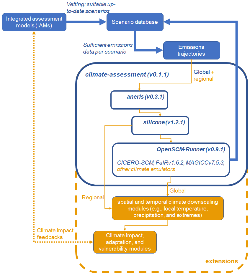
Figure 10 An overview of the current climate-assessment package (v0.1.1) and its workflow as applied for the IPCC AR6 mitigation scenarios climate, in blue. In orange are a few possible future extensions of this community climate-assessment workflow.

5.2 Scenario classification approaches

In AR6 and multiple previous IPCC assessments, scenarios were grouped to enable one to describe the characteristics of a group of scenarios (e.g. emissions reductions) that have a similar relevant feature (e.g. change in global mean surface temperature). Future scenario classifications can choose to review choices in two elements, namely (i) the chosen relevant feature and (ii) the tools used to evaluate how the chosen relevant feature relates to the scenario characteristic. When it comes to (i), one could for instance include other indicators beyond global temperature projections in the classification scheme when they are policy-relevant. This could include indicators of mitigation strategies, emissions trajectories, scenario and model design, other physical responses than global mean temperature, or climate impacts. In addition, the use of the median and the 33rd and 67th percentiles of global mean surface temperature for the classification in AR6, as well as the chosen specific warming levels, should not be seen as set in stone. For instance, one could choose to set the upper bound for category C3 to <1.8 ^∘C at 50 % probability rather than <2.0 ^∘C at 67 % probability. For (ii), AR6 WGIII used MAGICC to do the classification of scenarios. It would also be possible to use multiple climate emulators for classification, for instance by using a majority rule, a multi-model mean, or other ways of combining climate emulator distributions. In addition, the availability of information on multiple types of uncertainty (emissions, climate uncertainty within an emulator, multiple emulators) could be utilised to provide a confidence level of the assigned category classification.

Other aspects are the categorisation of scenarios and the use of descriptive statistics. Describing larger scenario categories comes with further limitations, because summary statistics can conceal the underlying distribution or overemphasise outliers. Further efforts could be made to describe key scenario characteristics by developing methods that correct for potential biases in the underlying scenario database, such as overrepresentation of scenarios from one specific modelling framework or weightings based on feasibility, historical compatibility, or scenario similarity (Guivarch et al., 2022). Other topics that might be relevant for a more multi-dimensional categorisation could be a separation of scenarios by their temperature decline after their peak or the associated reliance on net-negative emissions to achieve this.

5.3 Improving the understanding of the implications of overshoot

Related to the question of impact is the question of overshoot. From Fig. 5e–f we learn that each AR6 temperature category can be distinguished based on their ODY_1.5 time series, with almost all scenarios overshooting 1.5 ^∘C at least for a decade when using climate emulator MAGICC. Following the publication of the AR6 WGI, and much more strongly since the publication of AR6 WGII and WGIII, more focus has come on temperature overshoot. Many different peak-and-decline scenarios have been analysed in Chapter 3 of AR6 WGIII (Riahi et al., 2022), some with more pronounced overshoot than others. The discussion of overshoot in global climate policy is expected to be contentious due to its connection to the assumptions related to large-scale carbon dioxide removal or the potential that its presence in scenarios can delay strong mitigation policies while also potentially obscuring impact and feasibility risks of a temperature overshoot strategy (Maher and Symons, 2022; S. M. Smith, 2021). While overshoot indicators like ODY_1.5 may immediately be useful as an indicator to quantify differences in levels of overshoot between scenarios, further research is required to relate absolute levels of ODY to for instance climate impacts, loss and damage, and the risk of passing tipping points (Lenton et al., 2019) to be able to judge whether ODY or other temperature exceedance metrics could be a useful indicator to guide climate policies.

5.4 Climate-assessment workflow performance diagnostics and limitations and further development

In this paper, we have analysed the impact of changes in the climate-assessment workflow between SR1.5 and AR6. The changes made between the two assessments drew on an expert judgement of the applicability of available methods based on the available literature (Lamboll et al., 2020; Gidden et al., 2018, 2019), extensive knowledge of the AR6 scenario database, and experience from previous IPCC reports. To enable assessment of the climate outcomes of different climate-assessment workflow methods and to help determine whether such a change in methods is an improvement, a more systematic analysis is required. Such a more systematic analysis could involve establishing a reference case, specifying a set of “standard experiments” to be performed, and developing a set of diagnostics to evaluate the differences between method choices. In this paper, we have used GWP100, which is available in the AR6DB (Byers et al., 2022), to analyse the impact of the harmonisation and infilling of emissions trajectories. However, such an analysis is limited because it does not capture all climatically active species, like aerosols, and because GWP100 is only one out of multiple possible metrics. Alternative metric choices would not alter the climate outcome for a given GHG emissions pathway but could significantly affect the reported date on which net-zero GHG emissions are reached (Dhakal et al., 2022; Fig. 2 SM.10). Below, we will discuss two things. First, we point out a few ways to further investigate and improve the quality of the existing elements of the climate-assessment workflow as applied for AR6 WGIII. After that, we point out several remaining possible additions in detail and in scope for the development of the “climate-assessment” tool.

5.4.1 Improvements for harmonisation

This paper has analysed the changes in temperature estimates as the result of different methods using an ad hoc set-up. This set-up could serve as an inspiration for a future diagnostic tool and the development of benchmarks. Future work could consider extending or adjusting the decision tree currently available in aneris. For instance, to facilitate earlier convergence times, for CO₂ emissions in scenarios that reach and sustain net-zero CO₂ emissions, the decision tree could incorporate the convergence year dependent on the scenario design. A significant limitation of the harmonisation part of the workflow comes from the uncertainty in historical emissions and how such uncertainties and corrections are projected into the future. Harmonisation now collapses this uncertainty, sometimes updating emissions estimates that are out of date but other times forcing sets of estimates predicated on different measurements to agree with each other. In some cases, the trends of harmonised data can be markedly different to the trends in the original pathways – for instance, if historical emissions of an F-gas were overestimated but are projected to fall over time, the return to the original value can cause a net-positive gradient. Going forward, it would be worth investigating the impact of historical emissions choices and uncertainty on results.

5.4.2 Improvements for infilling

In a similar fashion, infilling performance can also be improved in a few different ways. One way would be to improve upon the infiller database, for instance by simply having a wider variety of modelled scenarios including especially aerosols and individual fluorinated gases, allowing for more differentiated infilled pathways. For some species, however, such as aerosols and ozone precursors, more research is needed to confidently select the most reasonable pathways or to infill a trajectory when it is missing. Another more advanced way would be to consider assigning weights to emissions trajectories in the scenario database. Lastly, and perhaps most influentially, future workflows could consider developing an automated infilling method decision tree for each emissions species. In AR6, two different methods and infiller databases are used, but always with the same lead gas, CO₂ from energy and industrial processes. For example, it may be preferable to let black carbon act as a lead component for infilling an organic carbon time series, when available.

5.4.3 The order of emissions processing steps

Another particular choice that could be evaluated in future work is the order of emissions processing. In AR6, following SR15, scenario vetting is done first, harmonisation second, and infilling (based on a harmonised set of emissions trajectories) last. Such a strategy ensures that the pathways that are infilled always start from a reasonable point and are influenced less by differences in historical emissions databases. Moreover, in this way two pathways that are identical except for when they were last harmonised should have the same infilled emissions. However, it would also be possible to do infilling before harmonisation, which would derive inter-species statistics used for infilling more directly from the modelled processes in the IAMs. This can only be guaranteed if they are infilled after harmonisation to the latest values. Lastly, by reducing the range of projections when using the QRW method, the risk of out-of-sample infilling is reduced.

5.4.4 Potential for further development of a community tool

The climate-assessment workflow is available as an installable open-source Python package with an MIT licence (Kikstra et al., 2022a). The code utilises functions of existing scientific software packages including “pyam” (Huppmann et al., 2021) and has been parallelised to enable one to do runs of many scenarios. It could be used as a community tool for scenario assessment that enables both easier access to well-calibrated climate emulators and the possibility of assessing a wider range of scenarios due to the possibility of infilling emissions trajectories. Such access to a climate-assessment tool can facilitate the development of socio-economic scenarios, for instance when new models only have the ability to model a limited number of emissions species. Results have already been used to allow for calculating the non-CO₂ contribution to warming, which is used to estimate the remaining carbon budget (Lamboll and Rogelj, 2022; Lamboll et al., 2022a).

There are many ways that the climate-assessment workflow could be extended and applied in future work. Some were already listed in Sect. 5.1.3 and visualised in Fig. 10. Here, we highlight additionally the possibility of connecting more climate emulators to this workflow as well as newer versions of already connected emulators through the “openscm” interface (Nicholls et al., 2022b). Firstly, to enable a robust assessment of climate mitigation pathways, a multi-emulator set-up is crucial for understanding both differences between the multiple models out there, including those that participated in RCMIP (Nicholls et al., 2021), and connecting to a common interface can enable easier intercomparisons. Secondly, having a wider set of simple climate models available and connected to this workflow could allow wider applications as the models differ in the detail and methods with which processes are modelled and thus also differ in which variables can be projected alongside scenarios.

6 Conclusions

The IPCC Sixth Assessment Report on the Mitigation of Climate Change (IPCC, 2022c) evaluated the climate outcomes of a very broad range of scenarios. This paper further documents and evaluates the climate-assessment workflow that allowed for this analysis and has further explored elements related to compatibility with the Paris Agreement, temperature overshoot, and the differences between climate emulators. The “climate-assessment” package introduced with this paper can serve as a tool that currently can support modellers in projecting climate outcomes of scenarios with emissions information, even if only several major emissions species were modelled. Future work could take this work as a start to further expand the coverage of the causal chain from emissions to climate impacts by extending the workflow beyond global climate characteristics toward regional or local climate change projections of temperature and precipitation and calculated climate impacts.