Determining the sensitive parameters of the Weather Research and Forecasting (WRF) model for the simulation of tropical cyclones in the Bay of Bengal using global sensitivity analysis and machine learning

The present study focuses on identifying the parameters from the Weather Research and Forecasting (WRF) model that strongly influence the simulation of tropical cyclones over the Bay of Bengal (BoB) region. Three global sensitivity analysis (SA) methods, namely, the Morris One-at-A-Time (MOAT), multivariate adaptive regression splines (MARS), and surrogate-based Sobol', are employed to identify the most sensitive parameters out of 24 tunable parameters corresponding to seven parameterization schemes of the WRF model. Ten tropical cyclones across different categories, such as cyclonic storms, severe cyclonic storms, and very severe cyclonic storms over BoB between 2011 and 2018, are selected in this study. The sensitivity scores of 24 parameters are evaluated for eight meteorological variables. The parameter sensitivity results are consistent across three SA methods for all the variables, and 8 out of the 24 parameters contribute 80 %–90 % to the overall sensitivity scores. It is found that the Sobol' method with Gaussian progress regression as a surrogate model can produce reliable sensitivity results when the available samples exceed 200. The parameters with which the model simulations have the least RMSE values when compared with the observations are considered the optimal parameters. Comparing observations and model simulations with the default and optimal parameters shows that simulations with the optimal set of parameters yield a 16.74 % improvement in the 10 m wind speed, 3.13 % in surface air temperature, 0.73 % in surface air pressure, and 9.18 % in precipitation simulations compared to the default set of parameters.

1 Introduction

The Indian subcontinent is vulnerable to tropical cyclones which develop in the North Indian Ocean (NIO) that consists of the Arabian Sea and the Bay of Bengal (BoB). These cyclones invariably cause widespread destruction to life and property. During the pre-monsoon and post-monsoon seasons, the tropical cyclones develop and bring heavy rainfall and gusts of wind towards the coastal lands (Singh et al., 2000). The number of tropical cyclones that form in the NIO has increased significantly during the past few years, specifically during the satellite era (1981–2014). The frequency and duration of very severe cyclones in the BoB were increasing at an alarming rate, which alone contributed to an overall increase in the frequency over the NIO (Balaji et al., 2018). An extensive study conducted using the past 30 years of data suggests that the severity of extremely severe cyclonic storms (ESCSs) over NIO increased by 26 %. The observed statistics reveal that the duration of the ESCS stage and maximum wind speeds of ESCSs have shown an increasing trend, and the landfall category was very severe (Singh et al., 2021a). On considering climate change, Singh et al. (2019) showed that the present warming climate impacts the formation and severity of the tropical cyclones over the BoB region. This ultimately affects the densely populated coastal cities adjacent to BoB, such as Chennai, Visakhapatnam, Bhubaneswar, and Kolkatta (Singh et al., 2019). Reddy et al. (2021) showed that projecting the present global warming conditions and climate changes into the near future leads to the intensification of the tropical cyclones with ESCS and very severe cyclonic storm (VSCS) categories. Consequently, accurate simulations of cyclone track, landfall, wind, and precipitation are critical in minimizing the damage caused by the tropical cyclones that are increasing in number and intensity. The Weather Research and Forecasting (WRF) model (Skamarock et al., 2008) is a community-based numerical weather prediction (NWP) system, which has been widely used to predict cyclones to date. The accuracy of the WRF model depends on (i) the specification of initial and lateral boundary conditions, (ii) the representation of model physics schemes, and (iii) the specification of parameters. With the availability of vast computational resources and observations, the accuracy in the specification of initial and lateral boundary conditions is improved to a great extent (Mohanty et al., 2010; Singh et al., 2021b). Many researchers have studied the sensitivity of physics schemes in simulating tropical cyclones over the BoB and invariably reported the performance of different combinations of physics schemes by comparing the tracks and intensities of cyclones (Pattanayak et al., 2012; Osuri et al., 2012; Rambabu et al., 2013; Kanase and Salvekar, 2015; Chandrasekar and Balaji, 2016; Sandeep et al., 2018; Venkata Rao et al., 2020; Mahala et al., 2021; Singh et al., 2021b; Messmer et al., 2021; Baki et al., 2021a). However, systematic studies on parameter sensitivity, to determine their optimal values, is yet to be explored for tropical cyclones over the BoB region.

Model parameters are the constants or exponents written in physics equations set up by the scheme developers, either through observations or theoretical calculations. In some cases, the default parameters are selected based on trial-and-error methods. This implies the parameters values may vary depending on the climatological conditions (Hong et al., 2004; Knutti et al., 2002). The WRF model consists of a bundle of physics schemes, and there exist as many as 100 tunable parameters (Quan et al., 2016). Calibration of all the parameters to reduce the model simulation error is highly challenging, and it brings several obstacles. First, a vast number of model simulations are required to perform parameter optimization, and the order goes beyond 10⁴ with an increase in parameter dimension. Second, the WRF model can simulate various meteorological variables, and each parameter may influence more than one variable. Thus, the parameter optimization needs to consider several variables simultaneously, which increases the computation cost even further (Chinta and Balaji, 2020). With the current situation and keeping in mind the availability of computational resources, performing thousands of numerical simulations for long periods such as tropical cyclones is extremely expensive. The best remedy is to use sensitivity analysis to identify the parameters that significantly impact the model simulation, thereby reducing the order of parameter dimension.

Sensitivity analysis is the method of uncertainty estimation in model outputs contributed by the variations in model inputs (Saltelli, 2002). Several researchers (Yang et al., 2012; Green and Zhang, 2014; Quan et al., 2016; Di et al., 2017; Yang et al., 2017; Ji et al., 2018; Wang et al., 2020; Chinta et al., 2021) have conducted sensitivity analyses of a number of parameters using various methods in the WRF model. Yang et al. (2012) conducted an uncertainty quantification and tuning of five key parameters found in the new Kain–Fritsch scheme of the WRF model, using the Multiple Very Fast Simulated Annealing (MVFSA) sampling algorithm. The authors have reported that the optimal parameters reduced the model precipitation bias significantly, and the model performance is sensitive to the downdraft and entrainment-related parameters. Green and Zhang (2014) conducted a sensitivity study to examine the influence of four parameters related to the fluxes of momentum and moist enthalpy across the air–sea interface, and they reported that the multiplication factors of flux coefficients control the intensity and structure of the tropical cyclones to a greater extent. Quan et al. (2016) examined the influence of 23 adjustable parameters on the WRF model to 11 atmospheric variables for the simulations of nine 5 d summer monsoon heavy precipitation events over the greater Beijing area, using the Morris One-at-A-Time (MOAT) method. The results showed that 6 out of 23 parameters were sensitive to most variables, and 5 parameters were sensitive to specific variables. Di et al. (2017) conducted sensitivity experiments of 18 parameters of the WRF model to the precipitation and surface temperature for the simulations of nine 2 d rainy events and nine 2 d sunny events, over greater Beijing. The authors have adopted four sensitivity analysis methods, namely, the delta test, the sum of trees, multivariate adaptive regression splines (MARS), and the Sobol' method. The results showed that five parameters greatly affected the precipitation, and two parameters affected surface temperature. Yang et al. (2017) studied the influence of 25 parameters within the Mellor–Yamada–Nakanishi–Niino (MYNN) planetary boundary layer scheme and MM5 surface layer scheme of the WRF model, for the simulations of turbine height wind speed, and reported that more than 60 % of the output variance is contributed by only six parameters. Ji et al. (2018) investigated the influence of 11 parameters on the precipitation and its related variables using the WRF model, for the simulations of a 30 d forecast, over China. The MOAT and surrogate-based Sobol' methods for the sensitivity analysis were used, and it was seen that the Gaussian process regression (GPR)-based Sobol' method was found to be more efficient than the MOAT method. The results also showed that four parameters significantly affect the precipitation and its associated quantities. Wang et al. (2020) studied the influence of 20 parameters on various meteorological and model variables, for 30 d simulations, over the Amazon region. The MOAT, MARS, and surrogate-based Sobol' methods for sensitivity analysis were employed; the results showed that the three methods were consistent, and 6 out of 20 parameters contribute to 80 %–90 % of the total variance. Chinta et al. (2021) studied the influence of 23 parameters on 11 meteorological variables for the simulations of twelve 4 d precipitation events during the Indian summer monsoon, using the WRF model. The sensitivity analysis was conducted using the MOAT method with 10 repetitions, and the results showed that 9 out of 23 parameters have a considerable impact on the model outputs. These studies show that hundreds of numerical simulations are required to perform sensitivity analysis. Thus, when selecting the sensitivity analysis methods and the number of parameters, the computational coast is a critical factor to consider.

Razavi and Gupta (2015) extensively studied the impact of numerous sensitivity analysis methods and reported that each method works based on a different set of ground-level definitions. The results from these methods do not always coincide. The studies proposed that while selecting a global sensitivity analysis method, one needs to consider four important characteristics, namely, (i) local sensitivities, (ii) the global distribution of local sensitivities, (iii) the global distribution of model responses, and (iv) the structural organization of the response surface. The studies also reported that relying on only one sensitivity analysis method may not yield feasible results since one single method may not be able to bring out all the characteristics fully. From these studies, one can infer that more than one SA method needs to be explored to improve confidence in the results obtained from sensitivity studies. The objective of the present study is to assess the influence of the WRF model parameters on various meteorological variables such as surface pressure, temperature, wind speed, precipitation, and atmospheric variables such as radiation fluxes and boundary layer height, for the simulations of tropical cyclones over the BoB region, using three different global sensitivity analysis methods.

This paper is organized as follows. A brief description of sensitivity analysis methods is presented in Sect. 2. Section 3 presents the design of numerical experiments and sensitivity experimental setup. Section 4 shows the results of the three sensitivity analysis methods and a comparison between simulations and observations, and Sect. 5 gives the summary and conclusions.

2 Sensitivity analysis methods

Sensitivity analysis is the assessment of uncertainties in model outputs that are attributed to the variations in inputs factors (Saltelli et al., 2008). The sensitivity analysis proceeds as follows: (1) selecting the right model and corresponding best set of physics schemes, (2) identifying the adjustable input parameters and corresponding ranges, (3) choosing the sensitivity analysis methods, (4) running the design of experiments to generate the sample set of input parameters and running the model using these parameter sets, and (5) analyzing the model outputs obtained by different parameter samples and quantifying the influence of selected parameters.

Sensitivity analysis methods are classified as derivative-based, response-surface-based, and variance-based approaches (Wang et al., 2020). In mathematical terms, the change of an output concerning the change in the input is referred to as the influence of that input, which is the principle of derivative-based SA. The Morris One-at-A-Time (MOAT) is a derivative-based SA method (see Sect. 2.1). The response-surface-based approach works on the differences between the responses of a mathematical model with all the input factors against that built with all but a particular input factor. The multivariate adaptive regression splines (MARS) method comes under this category (see Sect. 2.2). For the variance-based approaches, the influence of an input variable is defined as the contribution of the variance caused by that variable to the total variance of the model output. In mathematical terms, if the model output variance is decomposed by the contributions of each individual and combined interactions, then the highly sensitive factors will have a more significant variance contribution. The Sobol' sensitivity analysis comes under the variance-based approach (see Sect. 2.3). The MOAT method requires a uniform space-filling design, whereas the MARS and Sobol' methods require random space-filling designs. The MOAT and MARS methods give a more qualitative analysis, whereas the Sobol' method gives a quantitative analysis (Wang et al., 2020). As already stated by Razavi and Gupta (2015), unique sensitivity analysis methods for all applications are scarce in the literature. Furthermore, they observed that using more versatile SA methods could improve the confidence in sensitivity results by compensating for the drawbacks of the individual SA methods. Thus, in the present study, three widely used SA methods are selected for sensitivity analysis because of the differences in their methodology, as a consequence of which the parameters that are sensitive to the numerical model are studied. One can then extract those parameters which turn out to be significant in all the methods under consideration, thereby bolstering the argument. These are the most influential parameters that need to be worked out to improve the forecast skill.

2.1 The MOAT method

MOAT is a derivative-based sensitivity analysis method, also known as elementary effects method, which evaluates the parameter sensitivity according to the elemental effects of individual parameters (Morris, 1991). Consider a model with n input parameters $X=(x_{\mathrm{1}},x_{\mathrm{2}},\mathrm{\dots }{x}_n)$ with variability in their ranges. The parameters are normalized so that they lie in the range [0,1]. The parameter space is divided into p equally dispersed intervals, which can be filled with the discrete numbers of $[\mathrm{0},\frac{\mathrm{1}}{p-\mathrm{1}},\frac{\mathrm{2}}{p-\mathrm{1}},\mathrm{\dots },\frac{p-\mathrm{2}}{p-\mathrm{1}},\mathrm{1}]$. Here p is a user-defined integer. An initial vector of input parameter $X^{\mathrm{1}}=(x_{\mathrm{1}}^{\mathrm{1}},x_{\mathrm{2}}^{\mathrm{1}},\mathrm{\dots },x_n^{\mathrm{1}})$ is randomly created by taking values from the defined parameter space. Following the One-at-A-Time method, one parameter is selected and perturbed by Δ, i.e., $X_m^{\mathrm{1}}=(x_{\mathrm{1}}^{\mathrm{1}},x_{\mathrm{2}}^{\mathrm{1}},\mathrm{\dots },x_m^{\mathrm{1}}\pm \mathrm{\Delta },\mathrm{\dots },x_n^{\mathrm{1}})$. Here Δ is a randomly selected multiple of $\frac{\mathrm{1}}{p-\mathrm{1}}$. The model is run using these initial and perturbed vectors, and the elemental effect of that parameter is calculated as

$$\begin{array}{}\text{(1)}& {\text{EE}}_m^{\mathrm{1}}={\displaystyle \frac{f\left(X_m^{\mathrm{1}}\right)-f\left(X^{\mathrm{1}}\right)}{\mathrm{\Delta }}}.\end{array}$$

The subscript m implies the mth parameter is perturbed and the superscript 1 is the indication of first MOAT trajectory. In a single trajectory, this process is repeated for all parameters to compute the elementary effects of every parameter. The entire trajectory is replicated r times randomly to obtain the reliable sensitivity results. At the end of the process, a total of $r\times (n+\mathrm{1})$ model simulations are evaluated to complete the MOAT sensitivity analysis. A modified mean of $\left|{\text{EE}}_m\right|$, μ_m, and the standard deviation of $\left|{\text{EE}}_m\right|$, σ_m, are constructed as the sensitivity indices of input parameter x_m, as given below

$$\begin{array}{}\text{(2)}& {\displaystyle }{\mathit{\mu }}_{\mathrm{m}}=\sum _{i=\mathrm{1}}^r{\displaystyle \frac{\left|{\text{EE}}_m^i\right|}{r}},\text{(3)}& {\displaystyle }{\mathit{\sigma }}_m=\sqrt{{\displaystyle \frac{{\sum }_{i=\mathrm{1}}^r({\text{EE}}_m^i-{\mathit{\mu }}_{\mathrm{m}}{)}^{\mathrm{2}}}{r}}}.\end{array}$$

A high value of μ_m implies that the parameter x_m has a more significant impact on the model output. In contrast, a high value of σ_m indicates the nonlinearity of x_m or high interactions with other parameters.

2.2 The MARS method

MARS is an extension of Recursive Partition Regression model with the ability of continuous derivative (Friedman, 1991). The model is constructed by forward and backward passes: the forward pass divides the entire domain into a number of partitions and a overfitted model is produced by localized regressions in every partition, and the backward pass prunes the overfitted model to a best model by repeatedly removing least concerned basis function at a time. The MARS model can be decomposed as

$$\begin{array}{}\text{(4)}& \begin{array}{rl}\widehat{f}\left(x\right)& =a_{\mathrm{0}}{B}_{\mathrm{0}}+\sum _{m=\mathrm{1}}^M\sum _{\begin{array}{c}{K}_m=\mathrm{1}\\ i\in V\left(m\right)\end{array}}{a}_m{B}_m\left(x_i\right)\\ & +\sum _{m=\mathrm{1}}^M\sum _{\begin{array}{c}{K}_m=\mathrm{2}\\ (i,j)\in V\left(m\right)\end{array}}{a}_m{B}_m(x_i,x_j)+\mathrm{\dots }.\end{array}\end{array}$$

The basis functions can be a constant (B₀), a hinge function (B_m(x_i)), or a product of two or more hinge functions (B_m(x_i,x_j)). The coefficients $(a_{\mathrm{0}},a_{\mathrm{1}},\mathrm{\dots },a_m)$ are determined by linear regression in every partition. The generalized cross validation (GCV) score of every model during the backward pass is calculated as

$$\begin{array}{}\text{(5)}& \text{GCV}\left(m\right)={\displaystyle \frac{\mathrm{1}}{N}}{\displaystyle \frac{{\sum }_{i=\mathrm{1}}^N[y_i-{\widehat{f}}_m(X_i){]}^{\mathrm{2}}}{[\mathrm{1}-\frac{C\left(m\right)}{N}{]}^{\mathrm{2}}}}.\end{array}$$

Here N is the number of samples before pruning, y_i is the target data point, ${\widehat{f}}_m\left(X_i\right)$ is the mth model estimated data point corresponding to the input data X_i, and C(m) is the penalty factor accounting for the increase in variance due to the increase in complexity. The difference between the GCV scores of the pruned model with the overfitted model is measured as the importance of that parameter that has been removed. This implies that a higher difference indicates a higher influence of that parameter.

2.3 The Sobol' method

The Sobol' sensitivity analysis works on the basis of variance decomposition (Sobol, 2001). Consider a response function f(x) of a random vector x. The ANalysis Of VAriance (ANOVA) decomposition of f(x) is written as follows:

$$\begin{array}{}\text{(6)}& \begin{array}{rl}f\left(x\right)& =f_{\mathrm{0}}+\sum _{\mathrm{1}<i<n}{f}_i\left(x_i\right)+\sum _{\mathrm{1}<i,j<n}{f}_{ij}(x_i,x_j)+\mathrm{\dots }\\ & +f_{\mathrm{12}\mathrm{\dots }n}(x_i,x_j,\mathrm{\dots },x_n).\end{array}\end{array}$$

The variance of f(x) can be expressed as the contributions of variance of each term in Eq. (6), i.e.,

$$\begin{array}{}\text{(7)}& {\displaystyle }\begin{array}{rl}\int f^{\mathrm{2}}\left(x\right)\mathrm{d}x-f_{\mathrm{0}}& =\sum _{\mathrm{1}<i<n}\int f_i^{\mathrm{2}}\left(x_i\right)\mathrm{d}{x}_i\\ & +\sum _{\mathrm{1}<i,j<n}\int f_{ij}^{\mathrm{2}}(x_i,x_j)\mathrm{d}{x}_i\mathrm{d}{x}_j+\mathrm{\dots }\\ & +\int f_{\mathrm{12}\mathrm{\dots }n}^{\mathrm{2}}(x_i,x_j,\mathrm{\dots },x_n)\mathrm{d}{x}_{\mathrm{1}}\mathrm{d}{x}_{\mathrm{2}}\mathrm{\dots }\mathrm{d}{x}_n,\end{array}\text{(8)}& {\displaystyle }D=\sum _{\mathrm{1}<i<n}{D}_i+\sum _{\mathrm{1}<i,j<n}{D}_{ij}+\mathrm{\dots }+D_{\mathrm{12}\mathrm{\dots }n},\end{array}$$

where n is the total number of parameters, D is the total variance of output response function, D_i is the variance of x_i, D_ij is the variance of interactions of x_i and x_j, and D_12…n is the variance of interactions of all parameters. The Sobol' sensitivity indices of a particular parameter are defined as the ratio of individual variances to the total variance, and these can be written as

$$\begin{array}{}\text{(9)}& S_i={\displaystyle \frac{D_i}{D}};S_{ij}={\displaystyle \frac{D_{ij}}{D}};\mathrm{\dots }\text{ and }{S}_{\mathrm{12}\mathrm{\dots }n}={\displaystyle \frac{D_{\mathrm{12}\mathrm{\dots }n}}{D}}.\end{array}$$

These indices explain the effects of first-order, second-order, and total-order interactions, respectively. From Eqs. (8) and (9), it is evident that the sum of all the indices is equal to 1. Finally, the total-order sensitivity index of the ith parameter can be calculated as the sum of all the interactions of that parameter, i.e.,

$$\begin{array}{}\text{(10)}& S_{T_i}=S_i+S_{\begin{array}{c}ij\\ i\ne j\end{array}}+\mathrm{\dots }+S_{\mathrm{123}\mathrm{\dots }i\mathrm{\dots }n}.\end{array}$$

Generally, while the computation of first- and second-order effects is rather straightforward, the calculation of higher-order effects is very expensive, because the dimension of the higher-order terms is very large. To solve this problem, Homma and Saltelli (1996) introduced a new total sensitivity index as

$$\begin{array}{}\text{(11)}& S_{T_i}=\mathrm{1}-{\displaystyle \frac{D_{-i}}{D}},\end{array}$$

where D_−i indicates the total variance of response function without the consideration of the effects of the ith parameter. A higher total-order sensitivity index implies higher importance of that parameter.

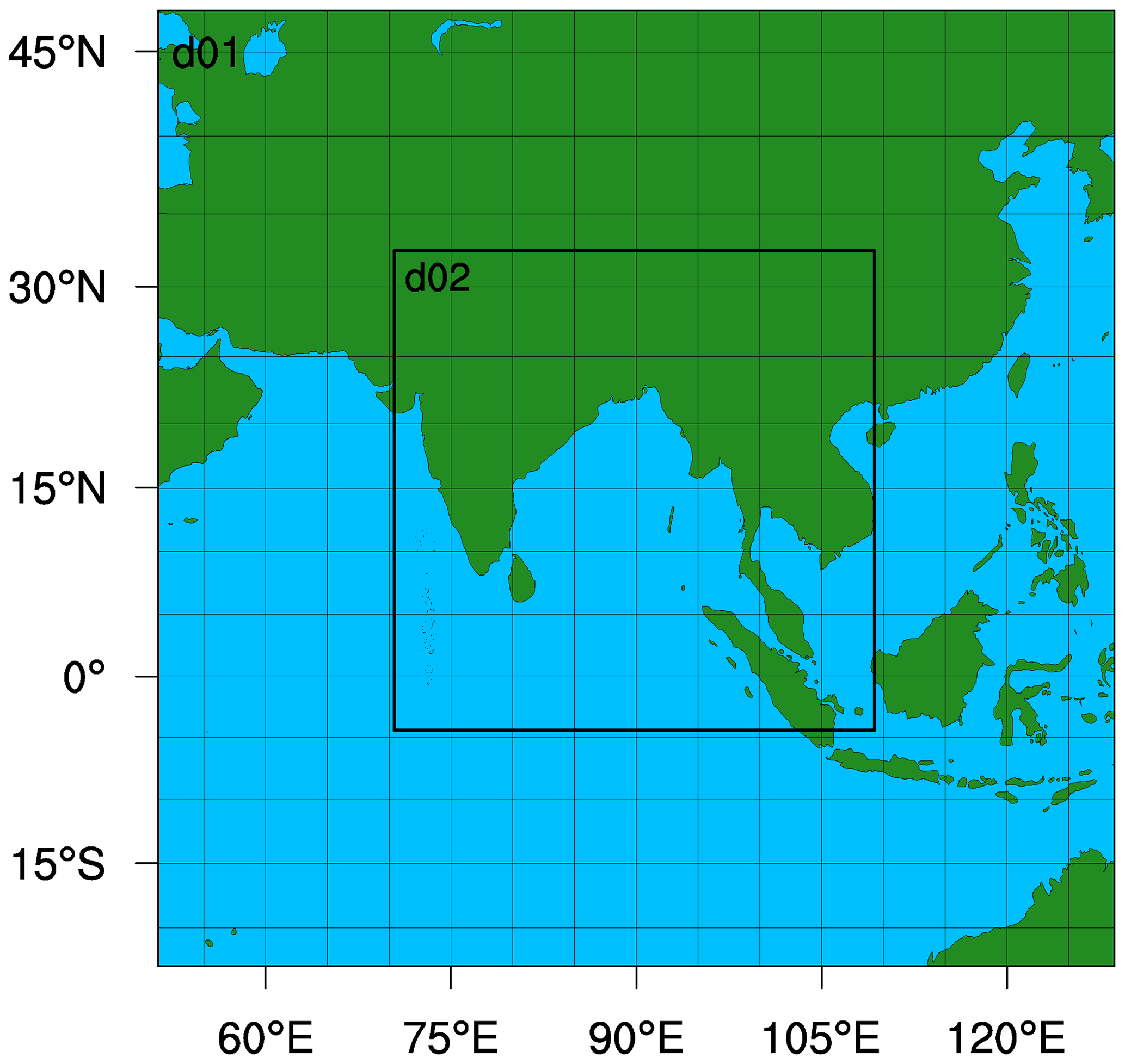
Figure 1 An illustration of the WRF model configuration with two nested domains.

3 Design of numerical experiments

3.1 WRF model configuration and adjustable parameters

In the present study, the Advanced Research WRF (WRF-ARW) model version 3.9 (Skamarock et al., 2008) is used for the numerical experiments. The model consists of two domains, d01 and d02, correctly aligning at the center, with a horizontal resolution of 36 and 12 km. The inner domain, which is our area of interest, consists of 360×360 grid points that encapsulate the BoB and cover the Indian subcontinent along with the northern Indian Ocean. The outer domain consists of 240×240 grid points and is kept reasonably away from the inner domain. The simulation domains are illustrated in Fig. 1. The model consists of 50 terrain-following σ layers in the vertical direction, while the top layer is kept at 50 hPa. The model is integrated with a time step of 90 and 30 s for domains d01 and d02, respectively. The NCEP FNL (National Centers for Environmental Prediction – Final) operational global analysis and forecast data at 1^∘ × 1^∘ resolution with a 6 h interval (National Centers for Environmental Prediction/National Weather Service/NOAA/U.S. Department of Commerce, 2000) are provided as the initial and lateral boundary conditions for the simulations. The simulations are carried out for 108 h, including 12 h of spin-up time.

Parameterization schemes represent the physical processes that are unresolved by the WRF model. The WRF model consists of seven different parameterization schemes: microphysics, cumulus physics, shortwave and longwave radiation, planetary boundary layer physics, land surface physics, and surface layer physics. The parameterization schemes used in this study are adopted from the studies of Baki et al. (2021a), which are rapid radiative transfer model (Mlawer et al., 1997) for longwave radiation, Dudhia shortwave scheme (Dudhia, 1989) for shortwave radiation, revised MM5 scheme (Jiménez et al., 2012) for surface layer physics, Unified Noah land surface model (Mukul Tewari et al., 2004) for land surface physics, Yonsei University (YSU) scheme (Hong et al., 2006) for planetary boundary layer physics, Kain–Fritsch (Kain, 2004) for cumulus physics, and WRF Single-Moment 6-class (WSM6) scheme (Hong and Lim, 2006) for microphysics. A total of 24 tunable parameters are selected based on the guidance from literature (Di et al., 2015; Quan et al., 2016; Di et al., 2020). The list of parameters and corresponding ranges are presented in Table 1. Though the selected parameter may not cover the entire existing parameters, the availability of computational resources limits the experimental design. The experimental design is based on the most critical parameters that are more likely to significantly influence the model output.

Table 1 Overview of the adjustable parameters and corresponding ranges selected in this study.

Table 2 Details of the tropical cyclones selected in this study.

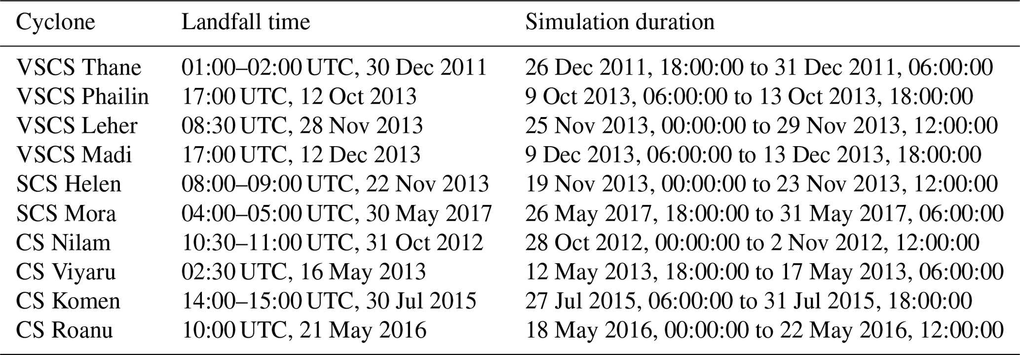
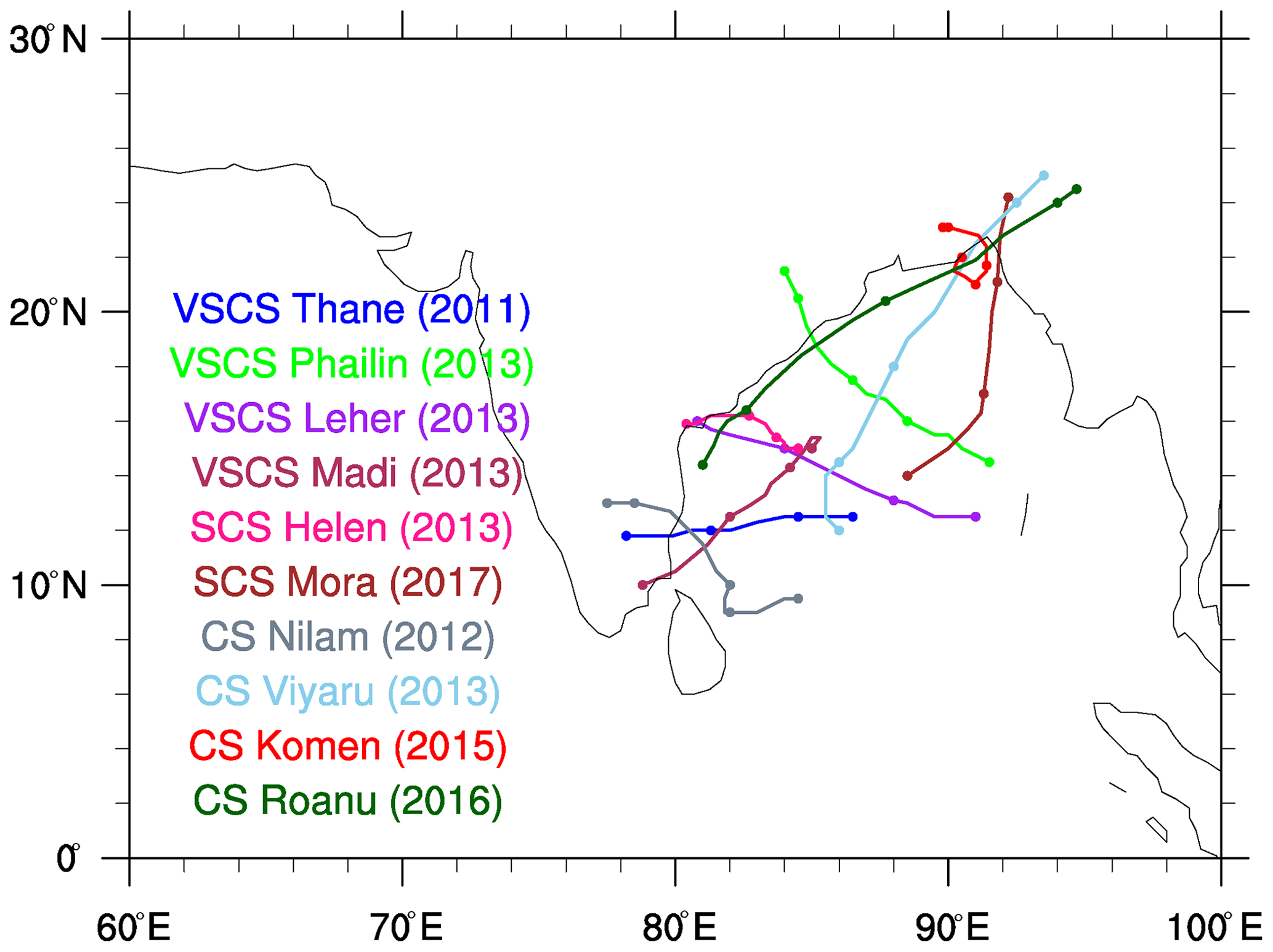
Figure 2 India Meteorological Department (IMD) observed tracks of the selected tropical cyclones.

3.2 Simulation events, WRF model output variables, and observational data

In the present study, 10 tropical cyclones that originated in the Bay of Bengal during the period of 2011 to 2017 are selected for the numerical experiments. The cyclones are chosen from various categories to generalize the experiments to ensure the robustness of the outcomes. The India Meteorological Department (IMD) categorizes the cyclones based on the maximum sustained surface wind speed (MSW) for a 3 min duration. The tropical cyclone categories used in this study are cyclonic storm (34–47 knots), severe cyclonic storm (48–63 knots), and very severe cyclonic storm (64–119 knots) (Srikanth et al., 2012). Figure 2 illustrates the IMD observed tracks of selected cyclones, with a clear indication of their category. Table 2 presents the details of category, landfall time, and the simulation duration of the cyclones selected in the present study. Each cyclone is simulated for 108 h, including 12 h of spin-up time, 72 h of simulation before the landfall, and 24 h of simulation after the landfall. The influence of parameters is conducted for different meteorological variables: wind speed 10 m above ground (WS10), temperature 2 m above ground (SAT), surface pressure (SAP), total precipitation (RAIN), planetary boundary layer height (PBLH), outgoing longwave radiation flux (OLR), downward shortwave radiation flux (DSWRF), and downward longwave radiation flux (DLWRF). The WRF simulations of these variables are stored at 6 h intervals.

The simulations are validated against the Indian Monsoon Data Assimilation and Analysis (IMDAA) data (Ashrit et al., 2020) and Integrated Multi-satellitE Retrievals for GPM (IMERG) dataset (Huffman and Savtchenko, 2019). The IMDAA data are available at 0.12^∘ × 0.12^∘ resolution with a 6 h latency, and the IMERG data are available at 0.1^∘ × 0.1^∘ resolution with a 30 min latency. Since the model resolution is close to the validation data resolution, it results in very little or no loss of data after regridding takes place. The accumulated precipitation data for validation are taken from IMERG data, while the remaining variables are taken from IMDAA data. Apart from these data, the maximum sustained wind speed (MSW) observations at the storm center for every cyclone, provided by the IMD at 3 h intervals, are also used for validation.

3.3 Experimental setup

The sensitivity analysis requires a large set of values of the parameters assigned to the WRF model, following which simulations are performed. Uncertainty Quantification Python Laboratory (UQ-PyL) is an uncertainty quantification platform, designed by Wang et al. (2016), which is used to generate the parameter samples for the MOAT method. Based on the studies of Quan et al. (2016), the parameter samples are generated with p=4 and r=10, which yields a total of $\mathrm{10}\times (\mathrm{24}+\mathrm{1})=\mathrm{250}$ parameter samples, for the selected 24 parameters. These parameter sets are assigned in the WRF model, and a total of $\mathrm{250}\times \mathrm{10}=\mathrm{2500}$ simulations are performed across 10 cyclones. Once the simulations are completed, the output meteorological variables are extracted and stored at 6 h intervals. The sensitivity indices for all the parameters are calculated based on Eqs. (2) and (3) which are implemented in UQ-PyL, and the indices are averaged over all the cyclones to generalize the results.

In contrast, the MARS and Sobol' methods require a different set of samples compared to the MOAT method. Based on the previous studies (Ji et al., 2018; Wang et al., 2020), the quasi-Monte Carlo (QMC) Sobol' sequence design (Sobol', 1967) is employed to create 250 parameter samples, using the UQ-PyL package for each event. Similar to the MOAT method, these parameter samples are assigned in the WRF model, and another 2500 simulations are performed for the cyclones under consideration. The output variables are extracted and stored at 6 h intervals. The evaluation of sensitivities using the MOAT method requires simulations only from the WRF model. In contrast, the MARS and Sobol' methods require skill score metrics between the simulation and observations. In the present study, the RMSE score between simulation and observation is employed as the skill score metric, which is formulated as

$$\begin{array}{}\text{(12)}& \mathrm{\text{RMSE}}=\sqrt{{\displaystyle \frac{\left[{\sum }_{l=\mathrm{1}}^L{\sum }_{k=\mathrm{1}}^K{\sum }_{j=\mathrm{1}}^J{\sum }_{i=\mathrm{1}}^I\right({\text{sim}}_{ijkl}-{\text{obs}}_{ijkl}{)}^{\mathrm{2}}]}{I\times J\times K\times L}}},\end{array}$$

where I and J are the number of grid points in lateral and longitudinal direction, K is the dimension of times, L is the number of cyclones, “sim” is the simulated value, and “obs” is the observed value. Since the same parameter set is employed for all the cyclones, Eq. (12) is employed to get one RMSE value corresponding to one parameter sample. The parameter set and RMSE are given as inputs and targets to the MARS solver, and the MARS sensitivity indices are computed following GCV Eq. (5).

The Sobol' method, as a quantitative sensitivity analysis method, gives more accurate and robust results, albeit at a much higher computational cost. The Sobol' method may require (10³ to ${\mathrm{10}}^{\mathrm{4}}\times (n+\mathrm{1})$) model runs (i.e., n is the number of parameters) to get accurate results. This is exceedingly challenging even if supercomputing facilities are available. To circumvent this difficulty, one can use the surrogate models instead of running the WRF model for more simulations. The surrogate models are powerful machine learning tools that can correlate the empirical relations between inputs (i.e., parameter set) and the targets (i.e., RMSE matrix). In the present study, five different surrogate models – namely, Gaussian process regression (GPR) (Schulz et al., 2018), support vector machines (SVMs) (Radhika and Shashi, 2009), random forest (RF) (Segal, 2005), regression tree (RT) (Razi and Athappilly, 2005), and k nearest neighbor (KNN) (Rajagopalan and Lall, 1999) – are selected for evaluation. The surrogate models are provided with the parameter set as inputs and the RMSE as the target, and the models are trained on these data. The goodness of fit is considered the accuracy metric, which is calculated as

$$\begin{array}{}\text{(13)}& R^{\mathrm{2}}=\mathrm{1}-{\displaystyle \frac{{\sum }_{i=\mathrm{1}}^N({\widehat{y}}_i-y_i{)}^{\mathrm{2}}}{{\sum }_{i=\mathrm{1}}^N(y_i-{\stackrel{\mathrm{‾}}{y}}_i{)}^{\mathrm{2}}}},\end{array}$$

where N is the total number of samples, y_i is the true value, ${\widehat{y}}_i$ is the predicted value, and $\stackrel{\mathrm{‾}}{y}$ is the mean of true values. The accuracy of the surrogate models is examined by applying 10-fold cross-validation, which is implemented as follows. The entire dataset is divided into 10 equally spaced subsets. The data in kth fold is kept as the test set, whereas the data from the remaining folds is taken as the training set. The surrogate model gets trained on this training set, and the simulations corresponding to the test set are estimated. This procedure is iterated for all folds, and the simulations of all folds are stacked into one set. This way, an entire simulation set corresponding to the test set is generated. These two sets are provided as simulations, and true values to Eq. (13) and the goodness of fit (R²) are calculated. The surrogate model with the highest R² value is selected as the best model. Once the best surrogate model is attained, the Sobol' sequence is used to generate 50 000 parameter samples, and the surrogate model predicts the corresponding outputs. Based on these outputs, the sensitivity indices are calculated. Pedregosa et al. (2011) have implemented the MARS method, Sobol' method, and the selected five surrogate models in Python language under the scikit-learn module, as application programming interfaces (APIs). The APIs of sensitivity methods and surrogate models are used in the present study.

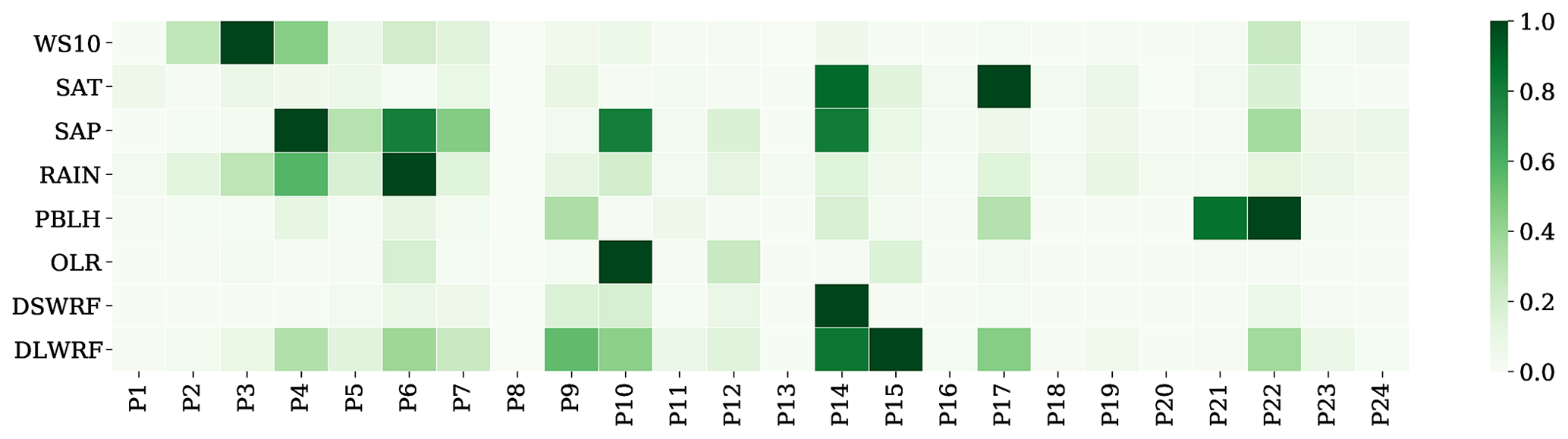
Figure 3 The heatmap of the normalized MOAT-modified means of 24 parameters for the meteorological variables considered, with one implying the most sensitive parameter and zero implying the least sensitive.

4 Results and discussion

4.1 MOAT sensitivity analysis

The sensitivity indices of parameters corresponding to the selected meteorological variables are calculated based on the MOAT method. The modified means of each variable under consideration are normalized to the range of [0,1]. They are illustrated as a heatmap in Fig. 3, with a darker shade indicating the highest sensitivity and a lighter shade indicating the least sensitivity. Figure 3 shows that parameter P14 has the highest influence on most of the variables, followed by parameter P6. The parameters P3, P4, P10, P15, P17, P21, and P22 also show high sensitivity to at least one of the variables. In contrast, the parameters P1, P8, P11, P13, P16, P18, and P20 do not seem to influence any one of the variables, and the remaining parameters have a minimal contribution. A close observation of Fig. 3 reveals that the variables OLR and DSWRF have the highest sensitivity to just one parameter each, whereas the remaining variables exhibit the highest sensitivity to at least two parameters.

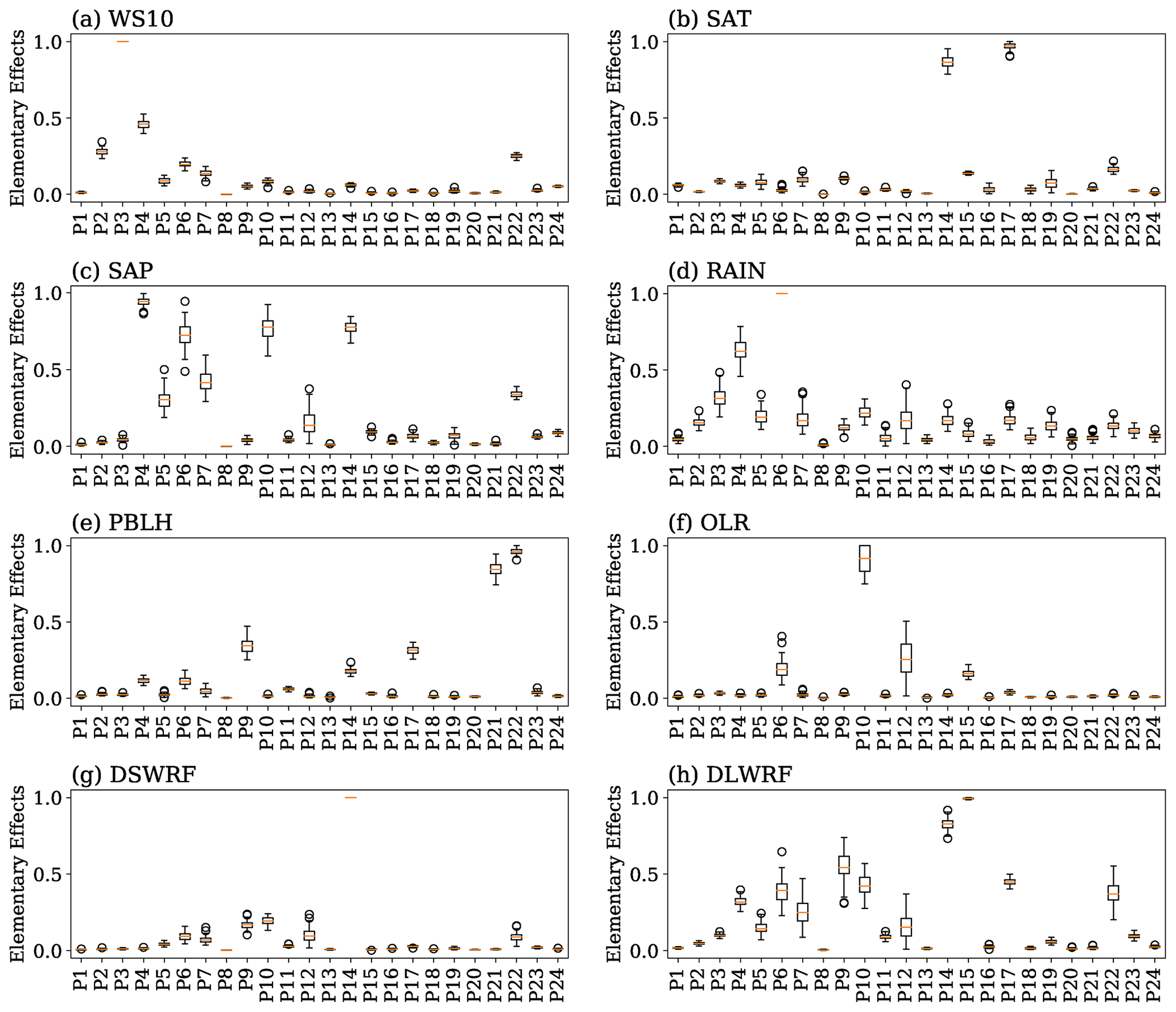
Figure 4 Boxplot of the elementary effects of 24 parameters for the meteorological variables considered. Each dataset is created with 100 applications of bootstrap resampling out of 10 instances. The center lines (red) are the median values; the top and bottom of the boxes are the average ±1 standard deviation; the upper and lower whiskers are the maximum and minimum values.

The uncertainties that lie in the sensitive parameters is examined by observing the distribution of the parameters. Since the available data points are limited to only 10 samples, a resampling method can be employed to procure more samples without further numerical model runs. The bootstrap resampling (Efron and Tibshirani, 1994) is an efficient way to generate the same number of samples as the original dataset, with replacement allowed. In the present study, the bootstrap method is employed for 100 applications to generate 10 samples with replacement. In this way, a new dataset of (100×10) is created for one parameter corresponding to one variable. The distribution of each parameter is illustrated as a boxplot in Fig. 4. In this figure, for every parameter, the horizontal red line inside the box indicates the median value, the upper and the lower bounds of the box are (mean ± 1 standard deviation value), and the upper and lower whiskers are the maximum and minimum values. The boxplot shows that the most sensitive parameters exhibit either a higher variance or a higher median value (Wang et al., 2020). For the variable OLR, Fig. 4f shows that the parameter P10 has the highest median value with large variance, whereas the parameters P6 and P12 have the least median values with large variances. Figure 4g shows that parameter P14 has the highest influence on the variable DSWRF and has a very minimal variance, whereas the influence of the remaining parameters is comparably very minimal. Figure 4c, e, and h show that the variables SAP, PBLH, and DLWRF have more than three sensitive parameters. The results show that except for DSWRF and OLR, all the variables have at least two high sensitive parameters. The results obtained by the boxplot strengthen the results obtained from the heat maps.

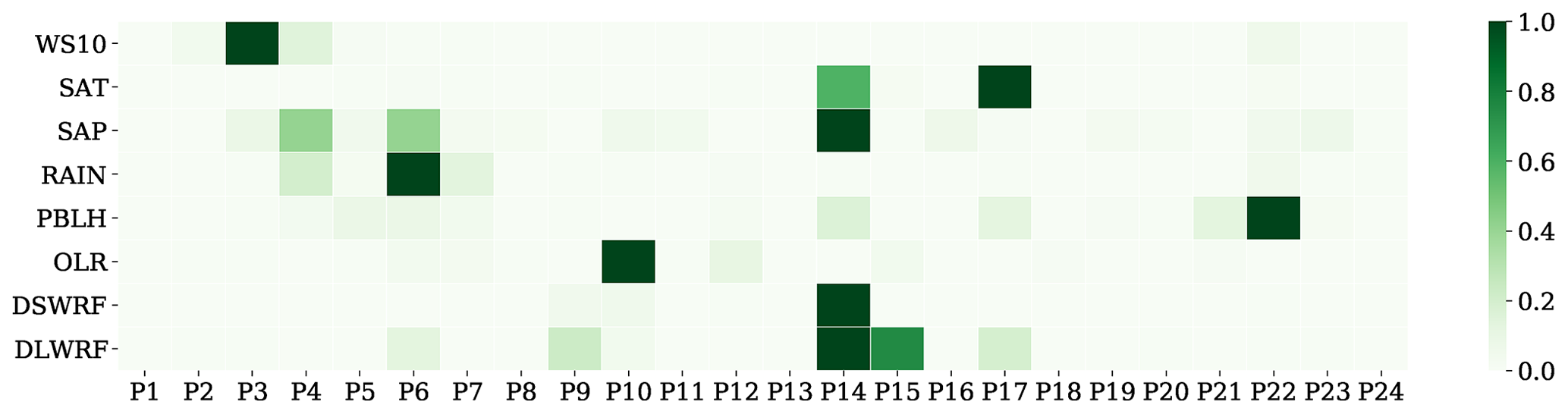
Figure 5 Heatmap of the normalized GCV scores of 24 parameters, for the meteorological variables considered, using the MARS method.

Figure 6 Boxplot of the normalized GCV scores of 24 parameters, for the meteorological variable considered, with the MARS method. Each dataset is created by 100 applications of bootstrap resampling out of 250 instances.

4.2 MARS sensitivity analysis

The GCV scores of 24 parameters corresponding to the selected variables are calculated based on the MARS method. Figure 5 illustrates the heatmap of normalized GCV scores, with 1 indicating the highest sensitivity and 0 indicating the least sensitivity. The intensity signatures of Fig. 5 are very consistent with that of Fig. 3. The results show that most of the variables are sensitive to P14, followed by parameter P6. In addition to this, the parameters P3, P4, P10, P15, P17, and P22 are seen to affect at least one of the dependent variables. The results also reveal that P1, P2, P8, P11, P13, P16, P18, P19, P20, P21, and P24 do not significantly influence any of the variables. A close observation of Fig. 5 reveals that the variables WS10, OLR, and DSWRF are sensitive to only one parameter each. In contrast, variables SAP, PBLH, and DLWRF are influenced by more than three parameters. The distribution of results is obtained by applying the bootstrap method, which is employed for 100 applications to generate 250 samples with replacement. In this way, a new dataset of (100×250) is created for one parameter corresponding to one variable. Figure 6 shows the boxplot of the MARS GCV scores generated by the bootstrap resampling dataset. Figure 6a, f, and g show that the variables WS10, OLR, and DSWRF are sensitive only to one parameter each. Similarly, Fig. 6c and h show that the variables SAP and DLWRF are sensitive to more than three parameters. The remaining variables are sensitive to at least two parameters. The results of the boxplot corroborate the results from the heatmap. These results are very consistent with that of the MOAT method.

4.3 Sobol' sensitivity analysis

The Sobol' method calculates the contribution of variation of the individual parameters to the total variance of the output by performing computations on a vast number of data. Thus, the Sobol' method is considered a quantitative analysis, which produces more reliable results. Due to the limitation of computational resources, a large number of model simulations are impractical to perform. The best remedy is to use surrogate models as an alternative to the original model, which can be trained on the limited samples produced by the original model, as already briefly mentioned. This implies that the Sobol' method's accuracy relies critically on the accuracy of the surrogate model. Thus, it becomes imperative to validate the surrogate model before analyzing the influence of the parameters.

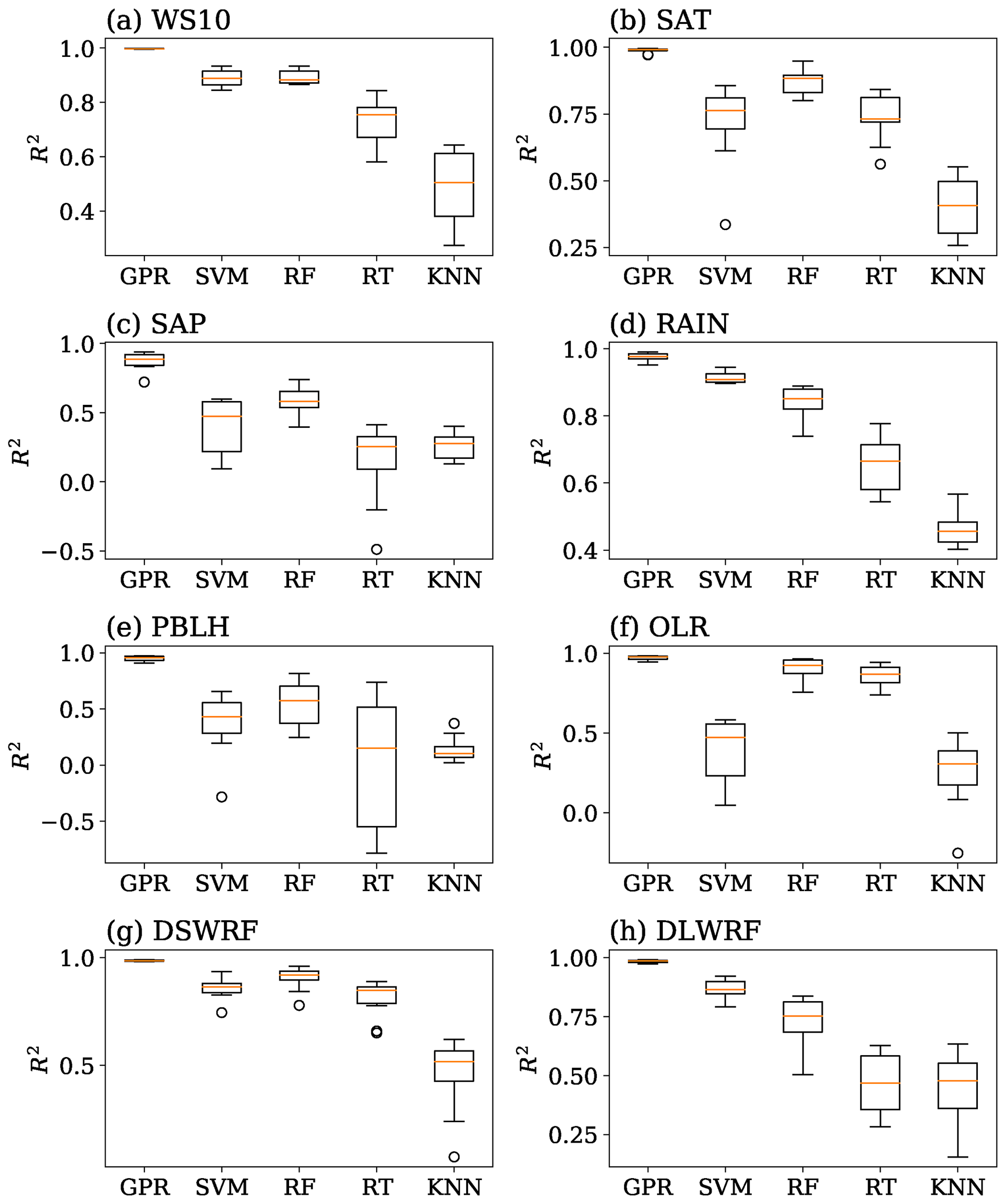
Figure 7 Cross-validation results of the surrogate models GPR, SVMs, RF, RT, and KNN for the meteorological variables considered in the present study.

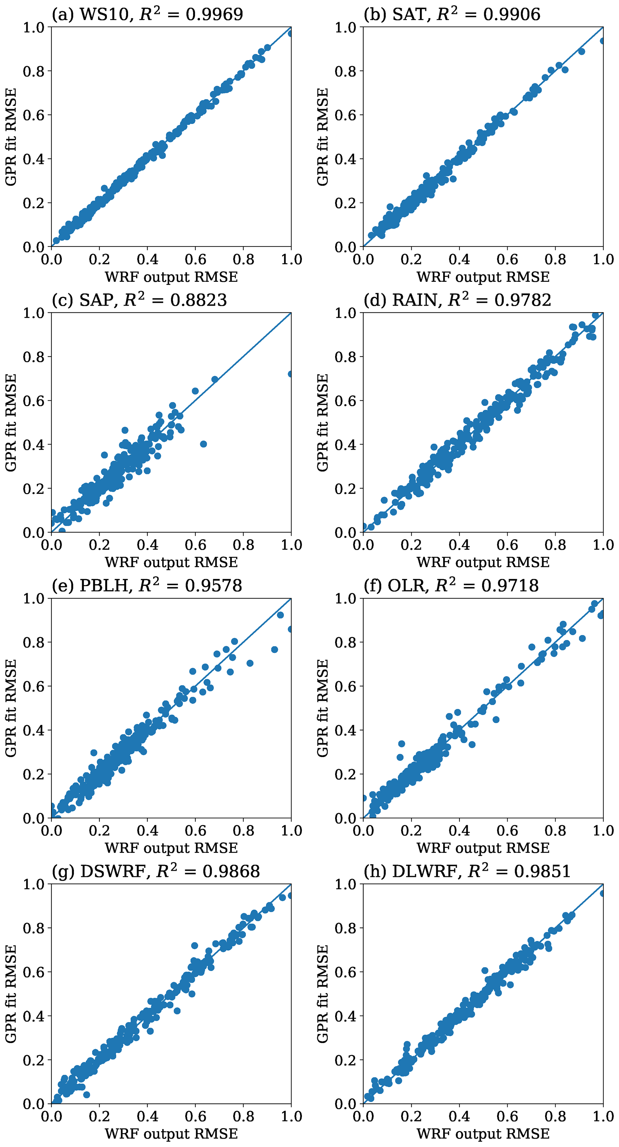
Figure 8 Accuracy of the GPR model for a sample size of 250 for the meteorological variables considered. Horizontal axis denotes the RMSE from WRF model and the vertical axis denotes the RMSE from GPR fit.

4.3.1 Validation of surrogate models

Figure 7 shows the distribution of R² scores of different surrogate models for the selected meteorological variables by applying bootstrap resampling. In Fig. 7, each panel corresponds to one meteorological variable, and the horizontal and vertical axes indicate the surrogate models and the goodness of fit (R²) value, respectively. For every meteorological variable, the GPR model has the highest R² value, which is close to 1, and the variance is also minimal. This implies that the GPR model can accurately correlate the empirical relations between inputs and outputs. In contrast, the remaining surrogate models show high variance in respect of at least one of the variables. Figure 7c shows that the regression tree has the highest variance with the least R² value, and the minimum whisker lies below zero, which indicates the inability of the RT in capturing the correlations. In every subfigure, the R² value of KNN is close to 0.5, which implies that the model can explain only 50 % of the total variance around its mean. The surrogate models SVM and RF have very close accuracy except for the variable OLR, in which the SVM shows high variance with R² value close to 0.5. These results indicate that all the remaining models have inconsistencies in their accuracy except for the GPR model. Figure 8 shows a scatterplot of the WRF model output against the GPR fit output for the eight variables under consideration. In Fig. 8, each panel corresponds to one meteorological variable, and the horizontal and vertical axes indicate the output of the WRF model and GPR fit, respectively. From the R² value shown in the plots, it is clear that the GPR model can explain 95 % of the variability of the output data around its mean, except for the variable surface pressure, for which the R² value is 0.88 (as shown in Fig. 8c). In view of the above, the GPR is chosen as the best surrogate model for the sensitivity studies with Sobol'.

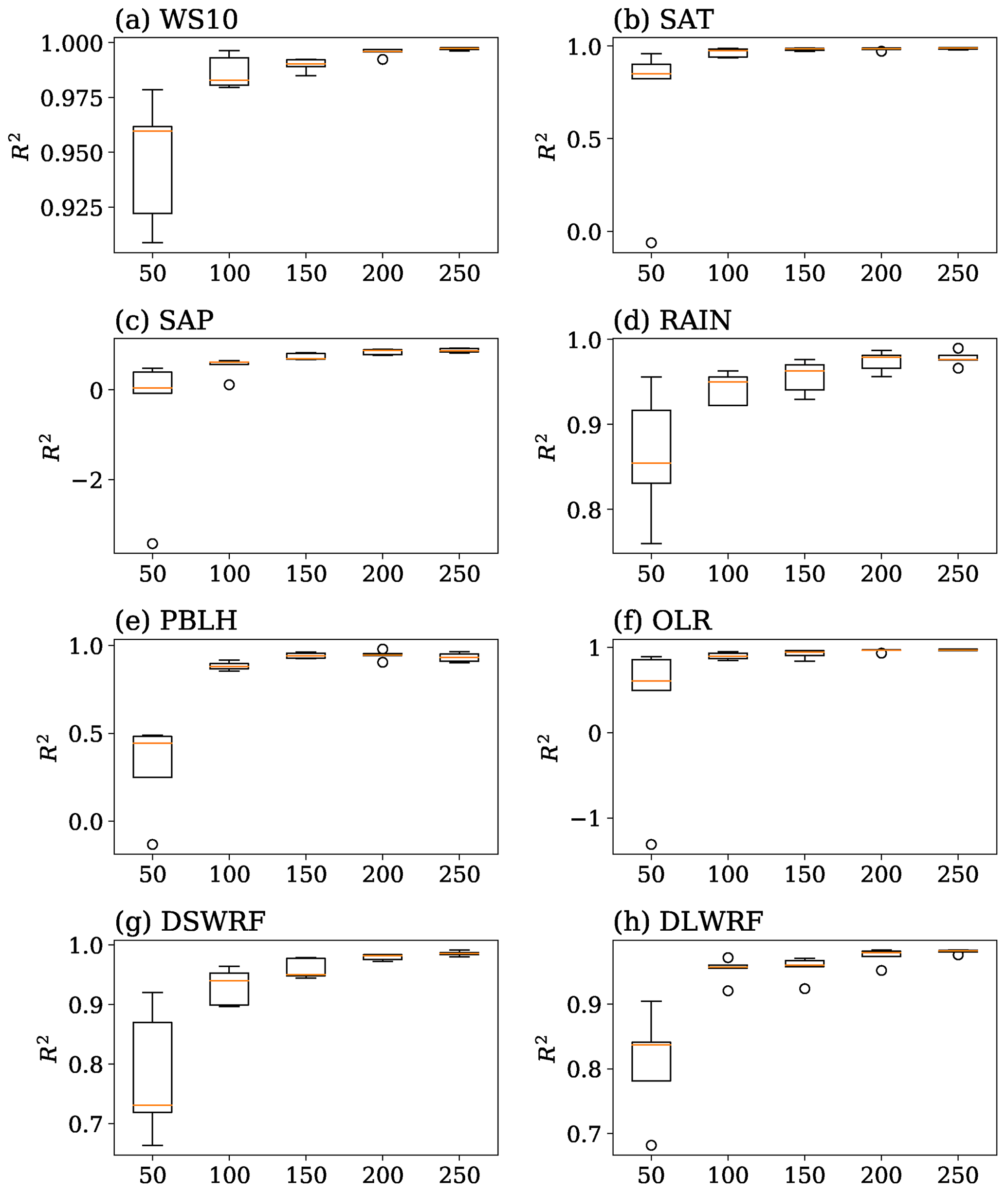
Figure 9 Cross-validation results of the GPR model with different sample sizes of 50, 100, 150, 200, and 250 for the meteorological variables considered.

4.3.2 Effects of sample size on surrogate model accuracy

The accuracy of a surrogate model depends on the number of samples provided to the model. At the same time, the sample size determines the computational cost required to perform additional model simulations. Thus, one needs to identify the minimum number of samples on which the surrogate model can attain reasonable accuracy. The effects of sample size on GPR's accuracy are evaluated as follows. The original dataset is divided into five sets: 50, 100, 150, 200, and 250 samples. Each set is bootstrap resampled for 100 instances, on which the accuracy of the GPR model is evaluated using 10-fold cross-validation. The distributions of R² values for different sample sizes are illustrated in Fig. 9, in which each panel corresponds to one meteorological variable. The abscissa and the ordinate indicate the number of samples and R² value, respectively. From this figure, it is evident that the accuracy of the GPR model increases monotonically with an increase in the sample size. The R² value has high variance at 50 and 100 sample sizes, whereas there is minimal variance found at 200 and 250 sample sizes. It is found that the sample sizes 200 and 250 have identical R² values, and there is little improvement found by increasing the samples beyond 200. Hence, based on the above results, it can be concluded that 200 samples are sufficient to construct a GPR model with adequate accuracy. Since the available data have 250 samples, the GPR model constructed with 250 samples is used in the Sobol' analysis.

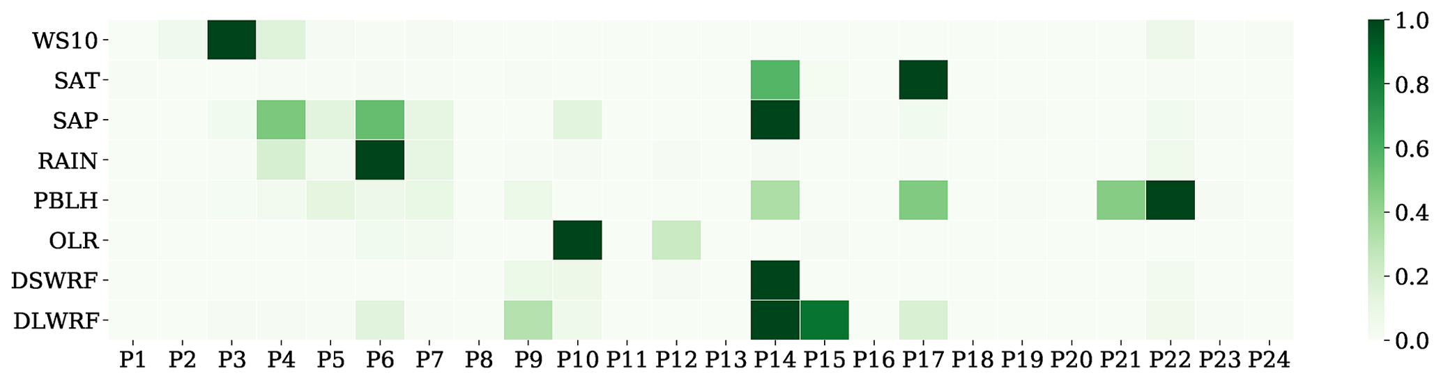
Figure 10 Heatmap of the total sensitivity index of 24 parameters for the meteorological variables considered, with the Sobol' sensitivity analysis.

4.3.3 Results of surrogate-based Sobol' method

The GPR model, which is built upon 250 samples, is used to predict the outputs of 50 000 samples generated by the Sobol' sequence, and these outputs are used to estimate the Sobol' sensitivity indices, corresponding to each variable. Figure 10 illustrates the heatmap of normalized total-order sensitivity indices, with 1 indicating the highest sensitivity and 0 indicating the least sensitivity, which is very consistent with the results of MOAT and MARS methods shown in Figs. 3 and 5 earlier. Parameter P14 is seen to be the most influential, followed by parameter P6. At least one of the dependent variables is sensitive to parameters P3, P4, P10, P15, P17, and P22. Comparing the results of the Sobol' method with MOAT and MARS methods, it is seen that the sensitivity patterns of each variable are showing consistency.

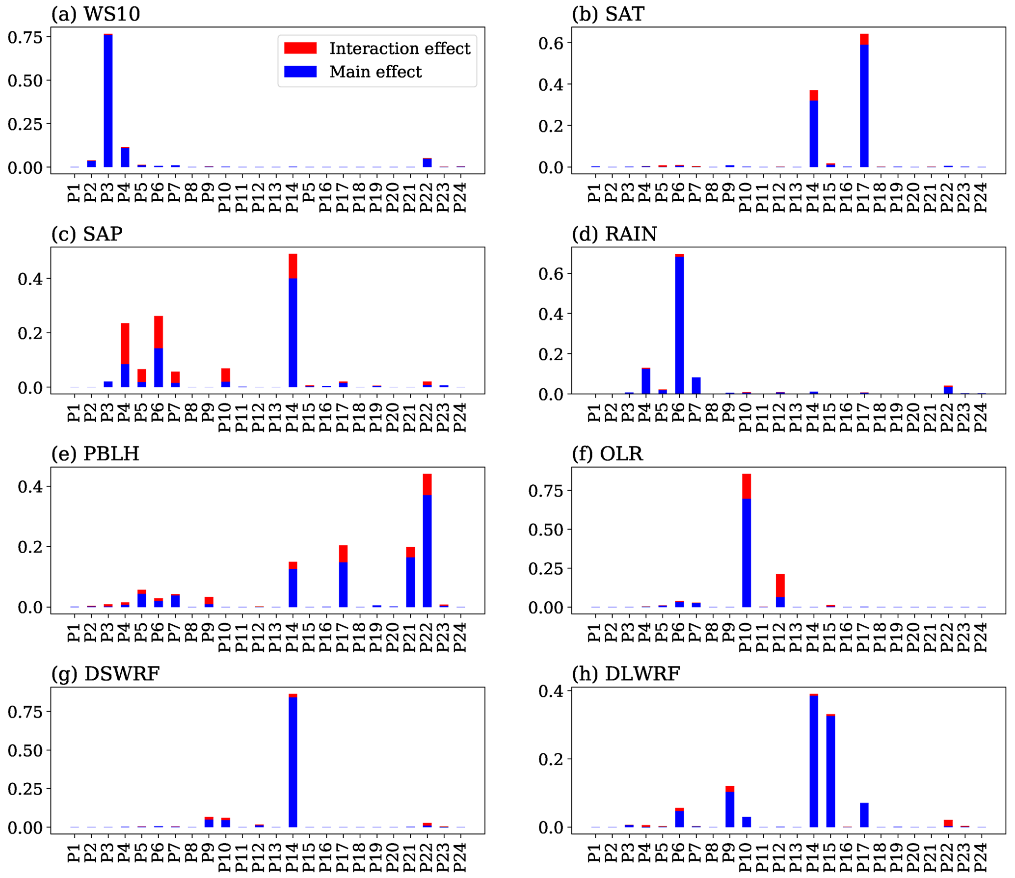
Figure 11 Sobol's primary and secondary effects of 24 parameters for the meteorological variables considered.

Figure 11a–h show the detailed illustration of the sensitivity indices of each meteorological variable. In each subfigure, the blue bar shows the first-order (primary) effects, the red bar shows the higher-order (interaction) effects, and the sum of these two show the total-order effects. The advantage of the Sobol' method is that the method can provide quantification of interaction effects. Figure 11c, e, and f show that the SAP, PBLH, and OLR have considerable higher-order effects, which indicate that the interactions are predominate in these variables. Figure 11b and g show that the variables SAT and DSWRF have only one sensitive parameter each, while Fig. 11c, e, and h show that the variables SAP, PBLH, and DLWRF are influenced by more than three parameters. These results strengthen the analogy obtained through the heatmap.

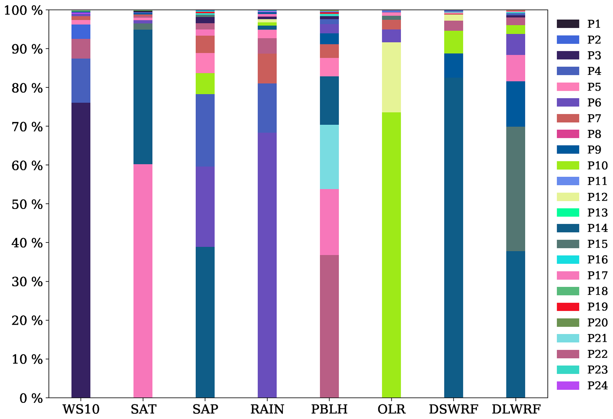
Figure 12 Accumulated relative importance of Sobol' total-order effects for different parameters, corresponding to each variable.

The results from the Sobol' method indicate that only a few parameters contribute much to the sensitivity of the output variables. Figure 12 shows the aggregate relative contribution of total-order effects of each parameter, corresponding to the selected variables. The abscissa indicates the output variables, and the ordinate indicates the relative importance, and the parameters are indicated by different colors. The figure shows that only 8 out of 24 parameters, namely, P3, P4, P6, P10, P14, P15, P17, and P22, are responsible for more than 80 % of the total sensitivity of every variable. Unlike MOAT or MARS methods, Sobol's deterministic nature gives more accurate results as they are free of any uncertainties.

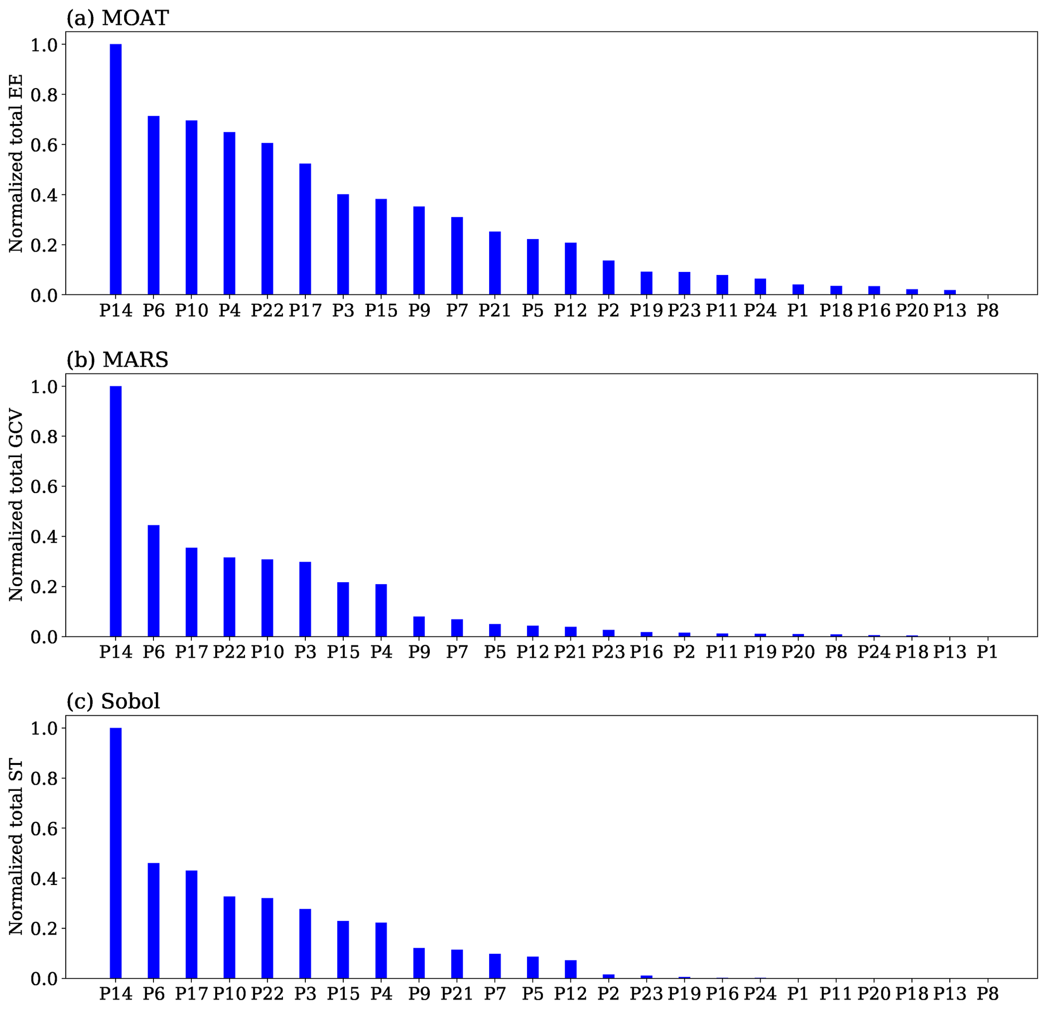
Figure 13 Ranks of the parameters according to their sensitivities based on (a) MOAT method, (b) MARS method, and (c) Sobol' method.

4.4 Physical interpretation of parameter sensitivity

The results obtained by the three sensitivity analysis methods suggest that only a few parameters strongly influence the meteorological variables under consideration in this study. The sensitivity indices of parameters obtained by the three methods are added over all variables and are normalized to [0,1]. The results are shown in Fig. 13 in descending order, which indicates the ranks of the parameters. Figure 13 shows that eight parameters, namely, P3, P4, P6, P10, P14, P15, P17, and P22, strongly influence the variables combined. Additionally, there is a near-exact matching of all the three sensitivity methods, with little variation in their ranks.

The results show that parameter P14 is the most influencing parameter among all. This represents the scattering tuning parameter used in the shortwave radiation scheme proposed by Dudhia (1989). This parameter is used in the downward component of solar flux equation (Montornès et al., 2015). This parameter is the main constant associated with the scattering attenuation and directly affects the solar radiation reaching the ground in the form of DSWRF. When a cloud is present in the atmosphere, it attenuates the downward solar radiation; simultaneously, it contributes to the downward longwave radiation by means of multiple scattering. Since the Dudhia (1989) scheme does not have a representation of the multi-scattering process, parameter P14 attenuates the downward radiation without any contribution to the heating rate (Montornès et al., 2015). This leads to changes in the DLWRF. The land surface model transforms the solar radiation into other kinds of energies, such as latent heat (LH) and sensible heat (SH) near the surface. This implies that the changes caused to the downward radiation will also affect the LH and SH. The planetary boundary layer is governed by the LH and SH. Therefore, the changes in the DSWRF will ultimately affect PBLH (Montornès et al., 2015). A higher value of P14 leads to a decrease in downward solar radiation and the surface level heating, which ultimately reduces the surface atmosphere temperature (SAT). Studies by Quan et al. (2016) show that the changes in SAT lead to variations in relative humidity. Due to the correlation between SAT, humidity, and SAP, variations in SAT and humidity lead to variations in the SAP.

The parameter P6 is the entrainment of mass flux rate in the Kain–Fritsch cumulus physics scheme, which has been identified as a sensitive parameter for the simulations of precipitation in the studies of Yang et al. (2012). This parameter determines the amount of ambient air entraining into the updraft flux, which further dilutes the updraft parcel. A high value of P6 indicates a high amount of ambient air entrainment into the air parcel. The entrainment of air into the updrafts indicates a detrainment of moisture from the updrafts, which is the important water source for the formation of stratiform clouds. This indicates that the formation of stratiform clouds compensates for the convective processes and leads to an increase in the stratiform precipitation (Liu et al., 2018). The occurrence of precipitation decreases the SAT and increases the relative humidity, leading to a change in the SAP. This parameter alters the formation of clouds, which in turn affects the variables that depend on clouds, such as OLR, DSWRF, and DLWRF (Quan et al., 2016; Ji et al., 2018). The parameter P17 is the multiplier of saturated soil water content used in the Unified Noah land surface scheme, proposed by Mukul Tewari et al. (2004). The saturated soil water content plays a prominent role in heat exchange between land and surface through moisture transportation in soil and evaporation. The SAT is affected by the amount of evaporation at the surface, which implies that changes in parameter P17 lead to SAT variations. The sensible heat and the latent heat are the two prime modes of heat exchange at the surface and for evaporation, on which the PBLH depends. Thus, parameter P17 also affects PBLH. Evaporation is the main constituent of cloud formation. Since parameter P17 affects evaporation, the DLWRF, which depends on clouds, will also be affected by P17.

Parameter P10 is the scaling factor applied for ice fall velocity used in the microphysics scheme, proposed by Hong et al. (2006). This parameter controls the ice terminal fall velocity, which governs the sedimentation of ice crystals. The cloud constituents such as cloud water and cloud ice are affected by the sedimentation of ice crystals. Since the cloud water and cloud ice reflect radiation into outer space, any change in parameter P10 causes variations in the OLR (Quan et al., 2016; Di et al., 2017; Ji et al., 2018). Parameter P4 is the von Kármán constant used in the surface layer scheme (Jiménez et al., 2012) and PBL scheme (Hong et al., 2006). This parameter relates the flow speed profile in a wall-normal shear flow to the stress at the boundary. This parameter directly influences the bulk transfer coefficient of momentum, heat, moisture, and diffusivity coefficient of momentum. This implies the changes in P4 will bring implicit variations in surface pressure and moisture, which lead to changes in the precipitation (Wang et al., 2020).

Parameter P22 is the profile shape exponent for calculating the moment diffusivity coefficient used in the PBL scheme. This parameter is directly related to P4 since both are used in the diffusivity coefficient of the momentum equation. This parameter regulates the mixing intensity of turbulence in the boundary layer, and because of this, the planetary boundary layer height (PBLH) will be affected (Quan et al., 2016; Di et al., 2017; Wang et al., 2020). Parameter P15 is the diffusivity angle for cloud optical depth computation used in the longwave radiation scheme, proposed by Mlawer et al. (1997). The longwave radiation irradiating back to the Earth's surface is attenuated by the diffusivity factor (which is the inverse of cosine of diffusivity angle) multiplied by the optical depth. Thus, changes in P15 directly cause variations in DLWRF (Quan et al., 2016; Di et al., 2017; Iacono et al., 2000; Viúdez-Mora et al., 2015). Parameter P3 is the scaling factor for surface roughness used in the surface layer scheme (Jiménez et al., 2012). A smooth surface lets the flow be laminar, whereas a rough surface drags the flow, thereby affecting the near-surface wind speed (Nelli et al., 2020). This way, parameter P3 is directly related to the wind speed. Thus, any changes in P3 results will also affect the surface wind speed (Wang et al., 2020).

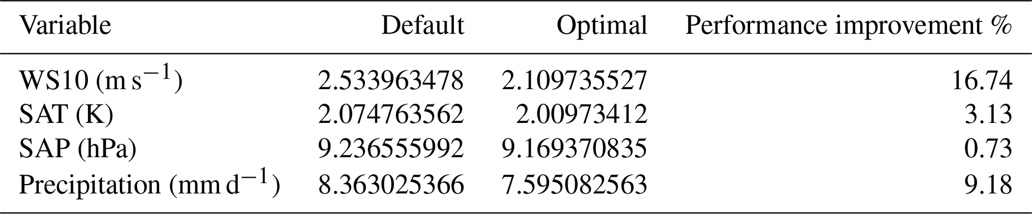
Table 3 RMSE values of variables simulated using default and optimal parameter sets.

4.5 A comparison between simulations with the default and optimal parameters

The objective of the present work is to identify the most important parameters which greatly influence the model output variables. In the present study, the parameters with which the model simulations show the least RMSE error with respect to the observations are selected as optimal parameters. However, these parameters can be further optimized by a procedure followed by Chinta and Balaji (2020) to improve the model simulations of output variables which are greatly affected by the parameters. To illustrate whether parameter optimization can improve model simulation, a comparison of WRF simulations with the default and optimal parameters for the meteorological variables, such as precipitation, surface temperature, surface pressure, and wind speed, was conducted. The RMSE values of WS10, SAT, SAP, and precipitation of the default and optimal simulations are evaluated and are shown in Table 3. The results show that optimal simulations have smaller RMSE values for surface wind (2.11 m s⁻¹) compared to default simulations (2.53 m s⁻¹). The percentage improvement is calculated as the percentage of reduction in RMSE score between the default and optimal simulations over the default simulations. Table 3 shows that a 16.74 % of improvement is achieved by using the optimal parameters over the default parameters for the simulations of surface wind speed. Similarly, the optimal parameters yield improvements of 3.13 % for surface temperature, 0.73 % for surface pressure, and 9.18 % for precipitation, over the default parameters.

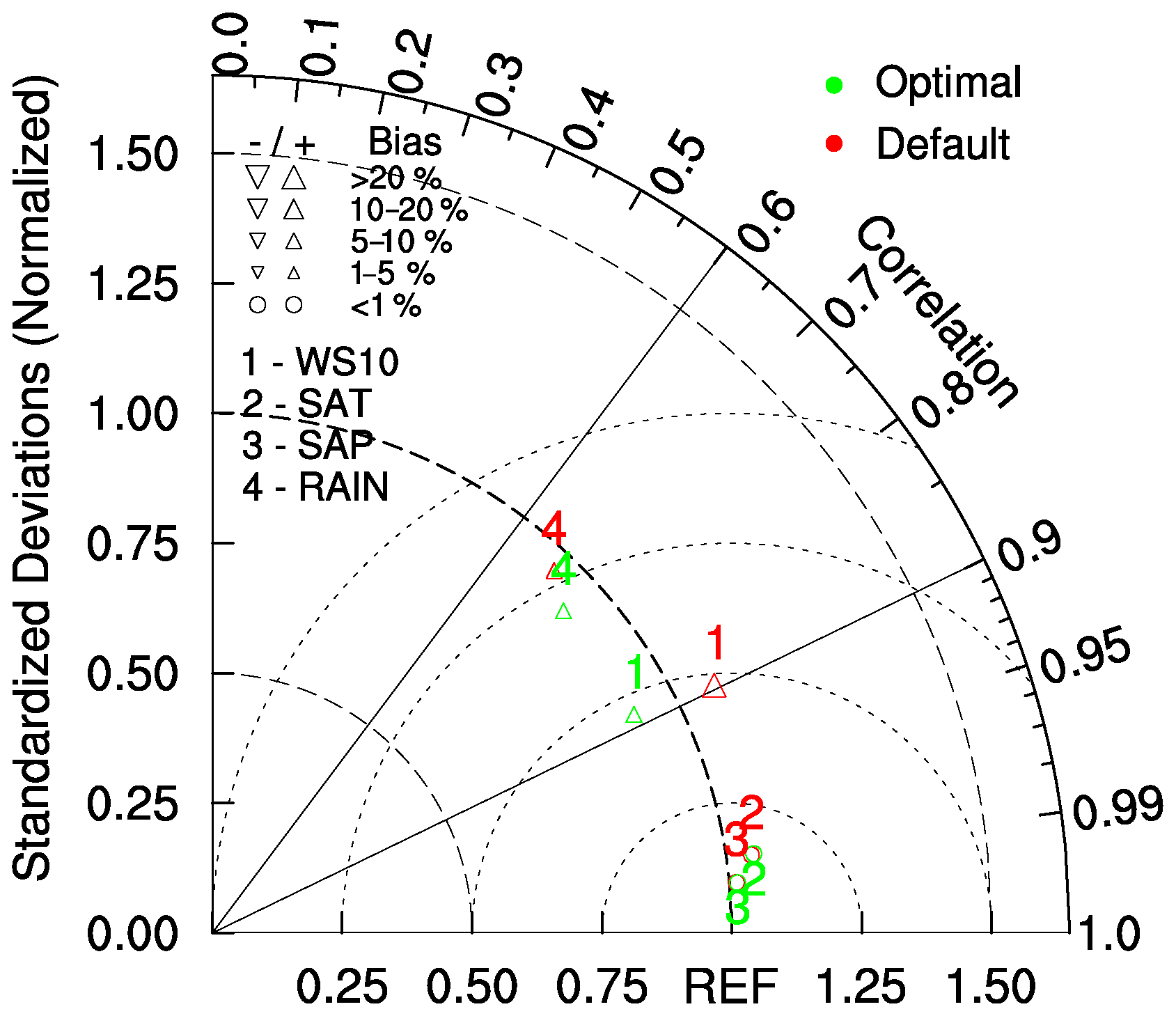
Figure 14 Comparison of Taylor statistics of WS10, SAT, SAP, and RAIN, simulated using the default and optimal parameters, averaged over all the cyclones for 3.5 d.

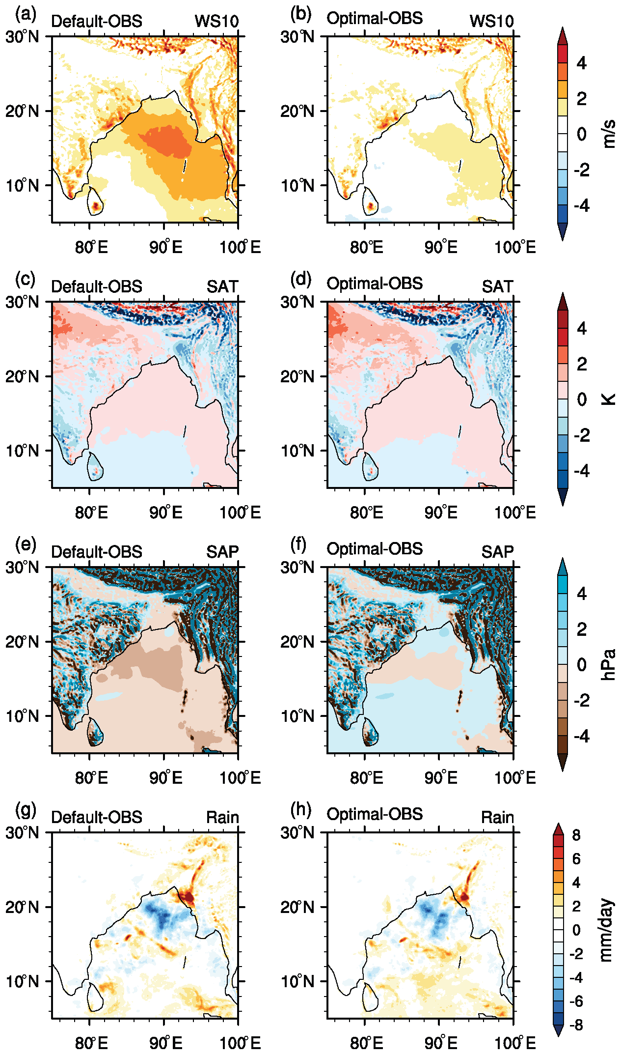
Figure 15 Comparison of the spatial distribution of meteorological variables simulated using default and optimal parameters, averaged over all the cyclones for 3.5 d. Surface wind bias (m s⁻¹) (a) between default and observations, (b) between optimal and observations, (c, d) surface temperature bias (K), (e, f) surface pressure bias (hPa), and (g, h) precipitation bias (mm d⁻¹).

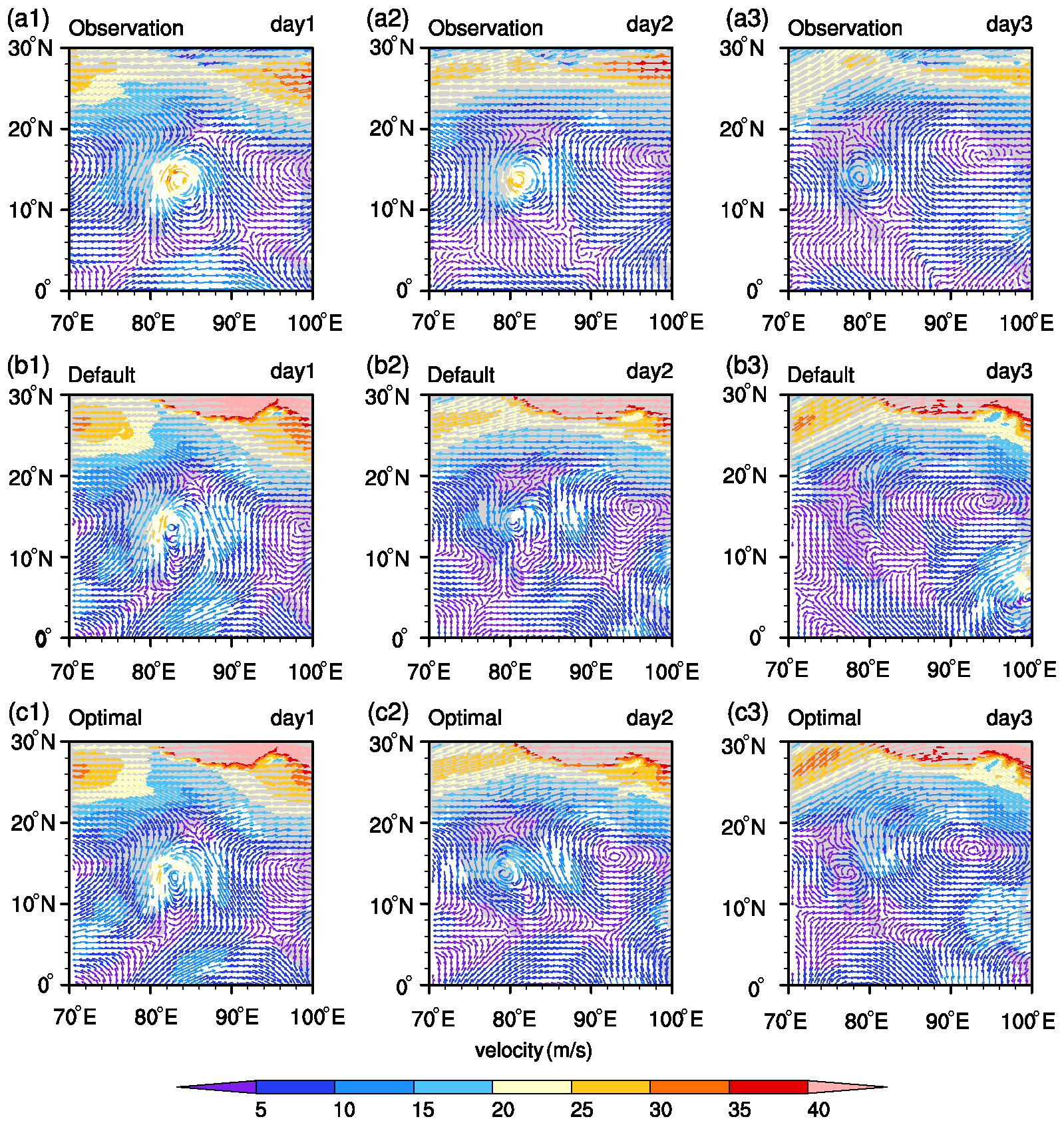
Figure 16 The wind velocity field at 500 hPa for the simulation of VSCS Thane using default and optimal parameters, compared with the observations. Panels (a1) to (a3) show observations at the end of day 1, day 2, and day 3; panels (b1) to (b3) show the simulations with default parameters; and panels (c1) to (c3) show the simulations with optimal parameters.

Taylor statistics (Taylor, 2001) are used to evaluate the accuracy of the model forecasts of WS10, SAT, SAP, and precipitation, simulated with the default and optimal parameters. The Taylor statistics consists of centered root-mean-square error, correlation coefficient, normalized standard deviation, and bias, which can be plotted in one Taylor diagram as shown in Fig. 14. The arcs centered at the origin represent the normalized standard deviation with the observed standard deviation located at the arc radius of 1. The simulation points close to the reference standard deviation arc imply that the variance in the simulations is similar to that of the observations. The arcs centered at the REF point on the abscissa represent the centered root-mean-square error (RMSE) with the observations. The simulation points close to the REF point indicate that the RMSE between the simulations and observations is very minimal. The correlation coefficient is the cosine of the position vector of a point, with zero being least correlated and one being highest correlated with the observation. The bias is the difference between the means of simulations and observations, which is merely indicated by up-pointing or down-pointing triangles on the plot. The points close to the REF point indicate the highest correlation, variance close to observations, and least RMSE, implying best performance. The default and optimal simulations of the SAT and SAP show no difference in any statistic, implying the similar performance of the parameters. The optimal and default simulations of WS10 are positioned midway to the reference standard deviation arc on either side, implying that the optimal simulations have less variance and that the default simulations have more variance compared to the observations, whereas the standard deviation is same for both. Both simulations lie on the same correlation vector and on the same semicircle originated from the REF point, implying that the simulations have the same centered RMSE and correlation coefficients. The main difference is seen in the overall biases, which lie in between 5 %–10 % for optimal simulations and 10 %–20 % for default simulations, implying the optimal parameters simulated WS10 with less bias. The optimal simulations of precipitation show less RMSE and high correlation compared to the default simulations. Even though the default simulations are positioned closer to the reference arc than the optimal simulations, the distance between the REF point and the optimal simulations is less compared to the default simulations, implying the best performance of the optimal parameters.

Figure 17 Same as Fig. 16 but for VSCS Phailin.

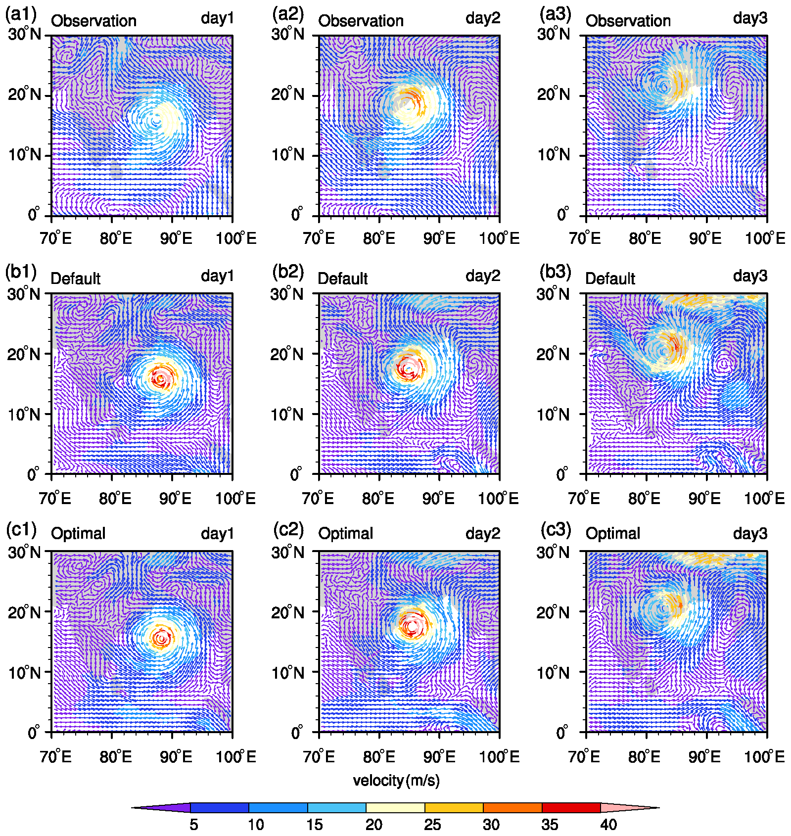
Figure 15 shows the domain-averaged spatial distributions of the bias in the variables evaluated as the difference between the simulations with the default set of parameters and the observations on the left panels, and the difference between the simulations with the optimal set of parameters and observations on the right panels. The IMDAA data are used to validate WS10, SAT, and SAP, and the IMERG rainfall data are used to validate precipitation. For surface wind speed, Fig. 15a and b show that the default simulations have large spatial coverage of 2, 3, and 4 m s⁻¹ positive bias over the Bay of Bengal region, whereas the optimal simulations have 2 m s⁻¹ bias over this region. The default and optimal simulations have similar spatial coverage over the land, whereas the optimal simulations show lesser bias compared to the default simulations, which is confirmed by Fig. 14. The surface plots clearly show that the optimal parameters improved the surface wind speed simulations compared to the default parameters. For surface temperature, Fig. 15c and d show that the default and optimal simulations have similar spatial distributions of temperature bias over the entire domain, with very minimal differences are observed over the northwest, southwest, and Bangladesh regions. Over these regions, the optimal simulations show a little less bias compared to the default simulations. For surface pressure, Fig. 15e and f show that the default and optimal simulations have similar spatial structures of bias over the entire domain with seemingly no variations at all. Figure 15g and h show that the default simulations have larger spatial structures with higher bias compared to the optimal simulations over the north BoB, Bangladesh coast, southeast BoB, and central BoB regions. These results indicate that the optimization of the sensitive parameters with respect to wind speed and precipitation will yield more improvement.

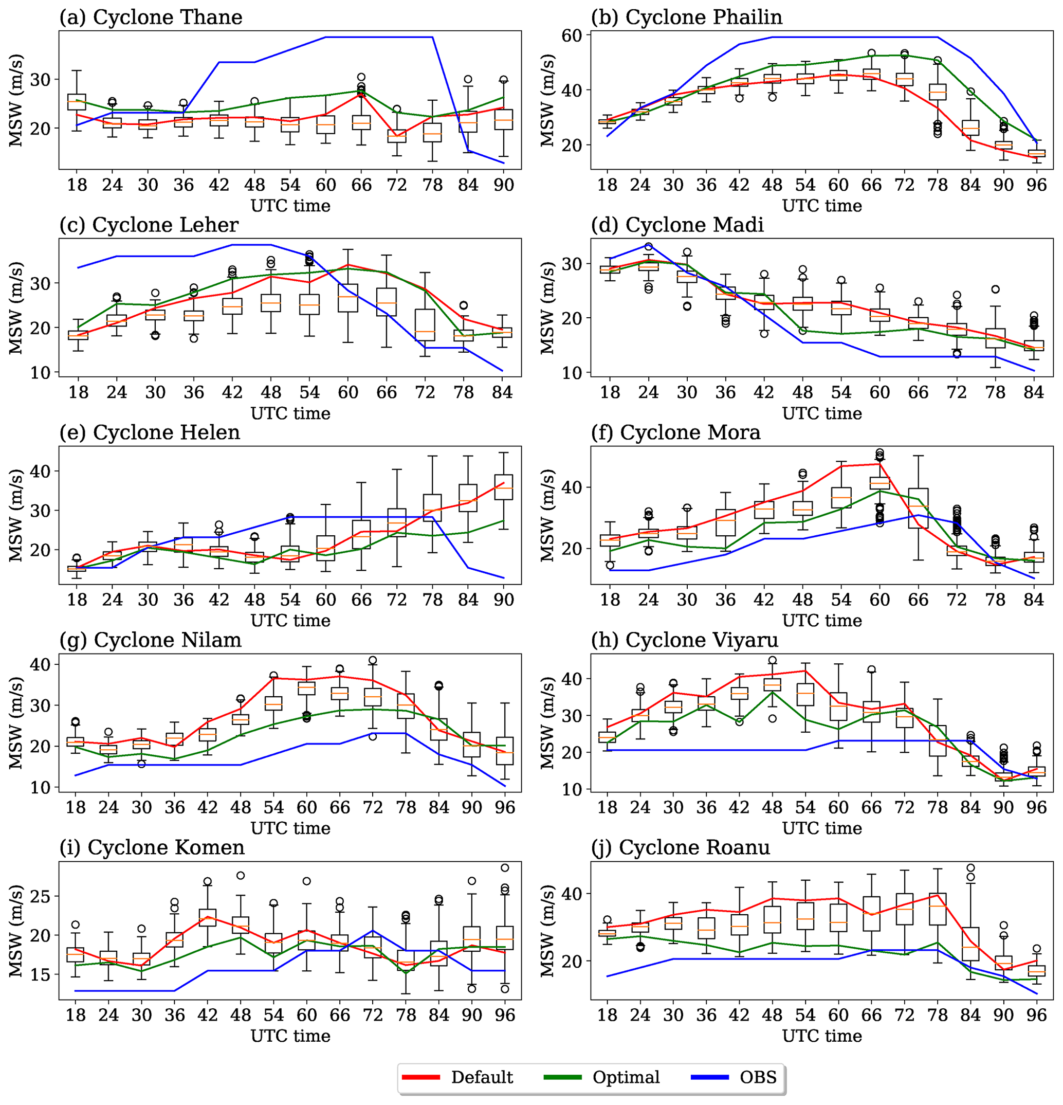
Figure 18 Comparisons of 3.5 d maximum sustained wind speed (MSW) of all cyclone simulations using the WRF model with the default and the optimal parameters. The boxplots of individual cyclones are obtained from the 250 simulations used for the MARS and Sobol' analysis. The green line shows the simulation with default parameters, the blue line shows the simulations with optimal parameters, and the red line shows the observed MSW. The data are collected at a 6 h interval and are plotted accordingly.

The WRF model runs with optimal parameters improved the simulations of meteorological variables at the surface level. However, the optimal parameters indeed exert an impact on the upper atmospheric variables, and the performance of optimal parameters for the simulations of variables at this level should be satisfactory to use in the future. For this purpose, the wind fields at 500 hPa of VSCS Thane and cyclone Phailin, simulated by the default and optimal parameters, are compared with observations, as shown in Figs. 16 and 17. For cyclone Thane, at the end of day 1, Fig. 16a1, b1, and c1 show that the default and optimal parameters simulated similar cyclonic circulations and traces of anticyclonic circulations that are matching with the observations well. At the end of day 2, Fig. 16a2, b2, and c2 show that the optimal parameters simulated a well-structured cyclonic circulation, whereas the default parameters simulated irregularities around the cyclonic circulation that were not observed. Both parameters simulated an anticyclonic circulation with a spatial deviation to that of the observed one. At the end of day 3, Fig. 16a3, b3, and c3 show that the default parameters simulated an anticyclonic circulation but failed to simulate a cyclonic circulation. In contrast, the optimal parameters simulated a well-structured cyclonic circulation with a spatial deviation and an anticyclonic circulation. For cyclone Phailin, at the end of day 1, Fig. 17a1, a2, and a3 show that the default and optimal parameters overestimated the cyclonic circulation intensity; however, the optimal simulations show relatively less intensity than the default simulations. At the end of day 2, Fig. 17a2, b2, and c2 show that default and optimal simulations have similar intense cyclonic circulations at the observed location with an overestimation compared to the observations. At the end of the day 3, Fig. 17a3, b3, and c3 show that the optimal simulations have relatively similar intensity compared to the observations than the default simulations. These results show that the optimal parameters simulated the velocity field at 500 hPa with less intensity and close to the observations than the default parameters.

The maximum sustained wind speed (MSW) is one of the primary measures of the intensity of a cyclone, and predicting an accurate MSW is of primordial importance for early warnings. In addition to the spatial distributions of variables, MSW is also compared for default and optimal simulations with boxplots as shown in Fig. 18. From the WRF simulations using QMC samples, MSW values of the 10 cyclones are extracted at 6 h intervals, beginning from the 18th hour till the observed time. Boxplots are generated for each cyclone using the data, and this shows that uncertainties in the parameters significantly affect the MSW simulations. The simulated MSW values with the default and optimal parameters are plotted along with the observed IMD MSW values, which show that the optimal simulations match quite well with the observations compared to the default simulations. The observations do not have to necessarily pass through the boxplots. In addition, the orange line in the boxplot indicates the mean of the MSW from the 250 simulations and represents the variability of the model simulations with respect to varying model parameters. The default or optimal simulations need not exactly pass through the mean but should lie within the limits of the boxplot, which is confirmed by the figure. These results indicate that the optimization of parameters will definitely improve the model simulations.

5 Conclusions

The present study evaluated the sensitivity of the eight meteorological variables, namely, surface wind speed, surface air temperature, surface air pressure, precipitation, planetary boundary layer height, downward shortwave radiation flux, downward longwave radiation flux, and outgoing longwave radiation flux, to 24 tunable parameters for the simulations of 10 tropical cyclones over the BoB region. The tunable parameters were selected from seven physics schemes of the WRF model. Ten tropical cyclones from different categories over the BoB between 2015 and 2018 were considered for the numerical experiments. Three sensitivity analysis methods, namely, Morris One-at-A-Time (MOAT), the multivariate adaptive regression splines (MARS), and the surrogate-based Sobol' were employed for carrying out the sensitivity experiments. The Gaussian process regression (GPR)-based Sobol' method produced better quantitative results with 200 samples. Parameter P14 (scattering tuning parameter used in the shortwave radiation) was seen to influence most of the output variables strongly. The variables surface air pressure (SAP) and downward longwave radiation flux (DLWRF) were found to be sensitive to most of the parameters. Out of the total selected parameters, eight parameters (P14 – scattering tuning parameter, P6 – multiplier of entrainment mass flux rate, P17 – multiplier for the saturated soil water content, P10 – scaling factor applied to ice fall velocity, P4 – von Kármán constant, P22 – profile shape exponent for calculating the momentum diffusivity coefficient, P3 – scaling related to surface roughness, and P15 – diffusivity angle for cloud optical depth) were found contributing to 80 %–90 % of the total sensitivity metric. A comparison of the WRF simulations with the default and that with optimal parameters with respect to observations showed a 19.65 % improvement in the surface wind simulation, 6.5 % improvement in the surface temperature simulation, and a 13.3 % improvement in the precipitation simulation when the optimal set of parameters is used instead of the default set of parameters. These results indicate that the optimization of model parameters using advanced optimization techniques can further improve the simulation of tropical cyclones in the Bay of Bengal.