Advanced parallel implementation of the coupled ocean–ice model FEMAO (version 2.0) with load balancing

In this paper, we present a parallel version of the finite-element model of the Arctic Ocean (FEMAO) configured for the White Sea and based on MPI technology. This model consists of two main parts: an ocean dynamics model and a surface ice dynamics model. These parts are very different in terms of the number of computations because the complexity of the ocean part depends on the bottom depth, while that of the sea-ice component does not. In the first step, we decided to locate both submodels on the same CPU cores with a common horizontal partition of the computational domain. The model domain is divided into small blocks, which are distributed over the CPU cores using Hilbert-curve balancing. Partitioning of the model domain is static (i.e., computed during the initialization stage). There are three baseline options: a single block per core, balancing of 2D computations, and balancing of 3D computations. After showing parallel acceleration for particular ocean and ice procedures, we construct the common partition, which minimizes joint imbalance in both submodels. Our novelty is using arrays shared by all blocks that belong to a CPU core instead of allocating separate arrays for each block, as is usually done. Computations on a CPU core are restricted by the masks of non-land grid nodes and block–core correspondence. This approach allows us to implement parallel computations into the model that are as simple as when the usual decomposition to squares is used, though with advances in load balancing. We provide parallel acceleration of up to 996 cores for the model with a resolution of $\mathrm{500}\times \mathrm{500}\times \mathrm{39}$ in the ocean component and 43 sea-ice scalars, and we carry out a detailed analysis of different partitions on the model runtime.

1 Introduction

The increasing performance and availability of multiprocessor computing devices make it possible to simulate complex natural systems with high resolution, while taking into account important phenomena and coupling comprehensive models of various subsystems. In particular, more precise, accurate, and full numerical descriptions of processes in seas and oceans have become possible. There are now models of seas that can simulate currents, dynamics of thermohaline fields, sea ice, pelagic ecology, benthic processes, and so on; see, for example, the review by Fox-Kemper et al. (2019).

The finite-element model of the Arctic Ocean (FEMAO; Iakovlev, 1996, 2012) has been developed since the 1990s and it has been adjusted to the White Sea (Chernov, 2013; Chernov et al., 2018). The model domain is a part of the cylinder over sphere (i.e., the Cartesian product of a region on the Earth's surface and a vertical segment). The coordinates are orthogonal, with the axes directed to the east, to the south, and downwards. The horizontal grid is structured and rectangular because finite elements are defined on triangles composing rectangles; see Iakovlev (1996). Points that correspond to the land are excluded from the computations using a mask of “wet” points. The z coordinate is used as the vertical axis. Therefore, for each 2D grid node, there are a number of actually used vertical layers. In the case of significantly variable depth, the number of levels also varies; see Fig. 1. In contrast, sea-ice and sea-surface computations are depth-independent. The presence of both 2D and 3D calculations complicates balancing of the computations for the full model.

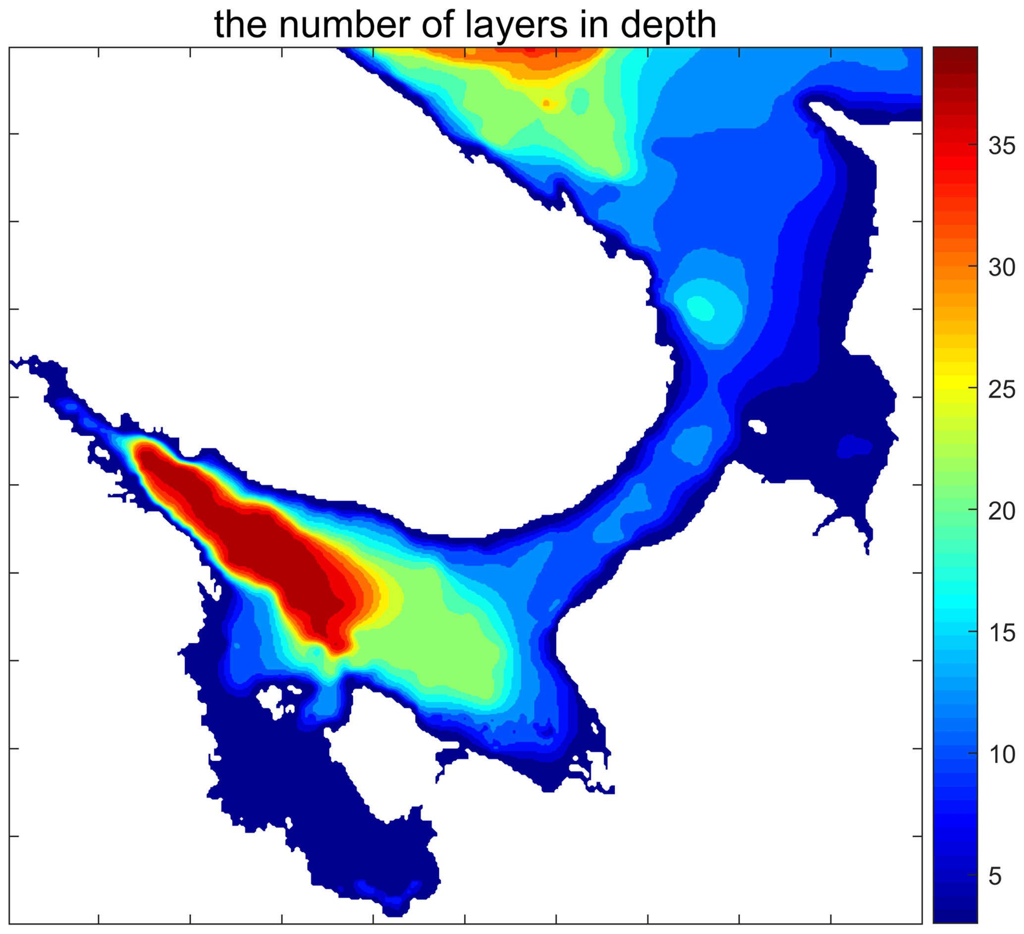
Figure 1 The number of depth layers in the White Sea model; the vertical grid step is 5 m up to 150 m deep and then 10 m up to 240 m.

The original code was written in Fortran 90/95, and it did not allow for computation in parallel. Our goal is to develop a parallel version of the model based on MPI technology without the need to make significant changes in the program code (i.e., to preserve loop structure and the mask of wet points but benefit from load balancing). Consequently, we developed a library that performs a partition of the 2D computational domain and organizes communication between the CPU cores.

In numerical ocean models, the baseline strategy is to decompose the domain into squares (Madec et al., 2008) or into small blocks, with consequent distribution over the processor cores (Dennis, 2007, 2003; Chaplygin et al., 2019). Both approaches preserve the original structure of the loops and utilize the direct referencing of neighboring grid nodes on rectangular grids. Decomposition into small blocks is more attractive from the viewpoint of load balancing, especially for z-coordinate models. Blocks can be distributed using the METIS (Karypis and Kumar, 1998) software or simpler algorithms, such as Hilbert curves (Dennis, 2007). Note that some modern ocean models can also benefit from unstructured mesh usage, whereby there is no need for the mask of wet points; see, for example, Koldunov et al. (2019a). In addition, some ocean models omit masking of wet points; see Madec et al. (2008). This implies an increase in the number of computations, but it benefits from fewer control-flow interruptions and gives rise to better automatic vectorization of loops.

In Sects. 2–4 we provide the model configuration and organization of the calculations in the non-parallel code on a structured rectangular grid. In Sect. 5 we describe the parallelization approach, which preserves the original structure of the loops. Domain decomposition is carried out in two steps: first, the model domain is divided into small blocks and then these blocks are distributed between CPU cores. For all blocks belonging to a given core a “shared” array is introduced, and a mask of computational points restricts calculations. Partitions could be of an arbitrary shape, but blocks allow us to reach the following benefits: a simple balancing algorithm (Hilbert curves) can be applied as the number of blocks along a given direction is chosen to be a power of 2, and boundary exchanges can be easily constructed for an arbitrary halo width smaller than the block size. In Sect. 6 we report parallel acceleration on different partitions for particular 2D and 3D subroutines and the whole model.

2 The White Sea

The White Sea is a relatively small (about 500 km×500 km) and shallow (67 m is the mean depth, with a maximal depth of no more than 340 m) semi-closed sea in the Arctic Ocean basin, located in the northwestern part of Russia and included in its territorial waters. Its area is 90 000 km². The White Sea plays an important role in the economy of the neighboring regions (Filatov et al., 2005).

The White Sea consists of several parts, including four bays and a narrow shallow strait called Gorlo that separates one part of the sea from the other. The coastline of the sea is quite complex, which means that the rectangle (almost a square) of the Earth's surface that contains the sea has only about one-third of the water area.

The White Sea is a convenient model region to test the numerical algorithms, software, and mathematical models that are intended to be used for the Arctic Ocean. First, a low spatial step and relatively high maximum velocities demand, due to the Courant stability condition, a rather small temporal step. This makes it difficult to develop efficient algorithms, implement stable numerical schemes, and ensure performance using the available computers. Second, because this model is less dependent on the initial data, it makes the test simulations easier because only the liquid boundary is needed to set the initial and boundary data. Finally, the White Sea's relatively small inertia enables us to check the correctness of the code with rather short simulations, which are able to demonstrate important features of the currents.

3 The model and the software

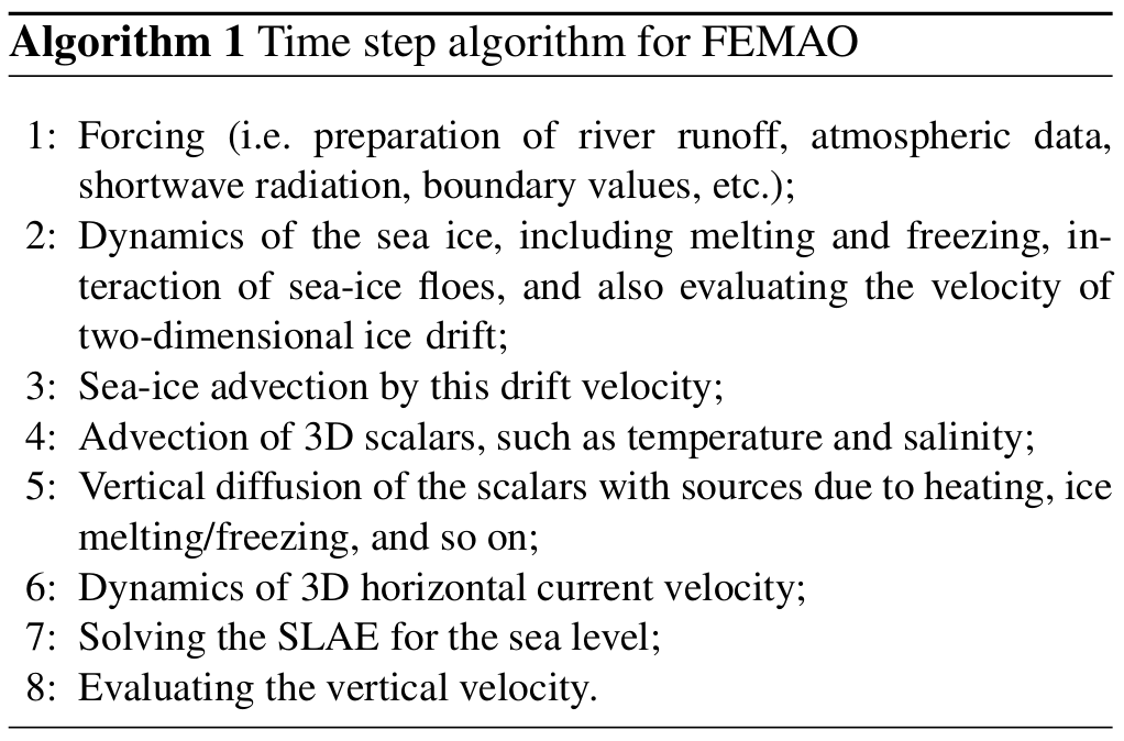
A time step in the FEMAO model consists of several procedures; see Algorithm 1. The model uses the physical process splitting approach so that geophysical fields are changed by each procedure that simulates one of the geophysical processes.

The matrix of the system of linear algebraic equations (SLAE) is sparse, and it contains 19 nonzero diagonals that correspond to adjacent mesh nodes within a finite element. The matrix does not vary in time, and it is precomputed before the time step loop. The most time-consuming steps for the sequential code version were 3D advection of scalars, 2D advection of sea-ice fields, and solving the SLAE for the sea level. The simple characteristic Galerkin scheme (Zienkiewicz and Taylor, 2000) is used for the 3D and 2D advection terms.

The local 1D sea-ice thermodynamics are based on the 0-layer model (Semtner, 1976; Parkinson and Washington, 1979) with some modifications in lateral melting and surface albedo (Yakovlev, 2009). There are 14 categories of ice thickness (gradations); the mechanical redistribution and the ice strength are identical to the CICE (Hunke et al., 2013). The elastic–viscous plastic scheme (EVP; Danilov et al., 2015) with a modification for the relaxation timescales (Wang et al., 2016) is used for the sea-ice dynamics (see also Appendix 3 in Koldunov et al., 2019b). Sea ice is described by the distribution of its compactness (concentration) and ice volume for each gradation. In addition, the snow-on-ice volume for each gradation is evaluated. Therefore, there are 43 2D sea-ice scalars: ice and snow volume for 14 gradations and sea-ice compactness for 15 gradations (including water). Because there are 39 vertical layers in an ocean component, the set of all of the sea-ice data is comparable to a single 3D scalar.

The tested version of the model has a spatial resolution of 0.036^∘ E, 0.011^∘ N, which is between 1.0 and 1.3 km along parallels and 1.2 km along a meridian. The number of 2D grid nodes is 500×500, and only 33 % of them are wet (84 542). The time step is 100 s. The vertical step is 5 m up to 150 m deep and then 10 m up to 300 m. In fact, in the bathymetry data (ETOPO; Amante and Eakins, 2009) the deepest point of the sea is shallower than it really is, which reduces the actual maximum depth to 240 m. Comparison of available bathymetry data for the White Sea is given in Chernov and Tolstikov (2020) in Table 1.

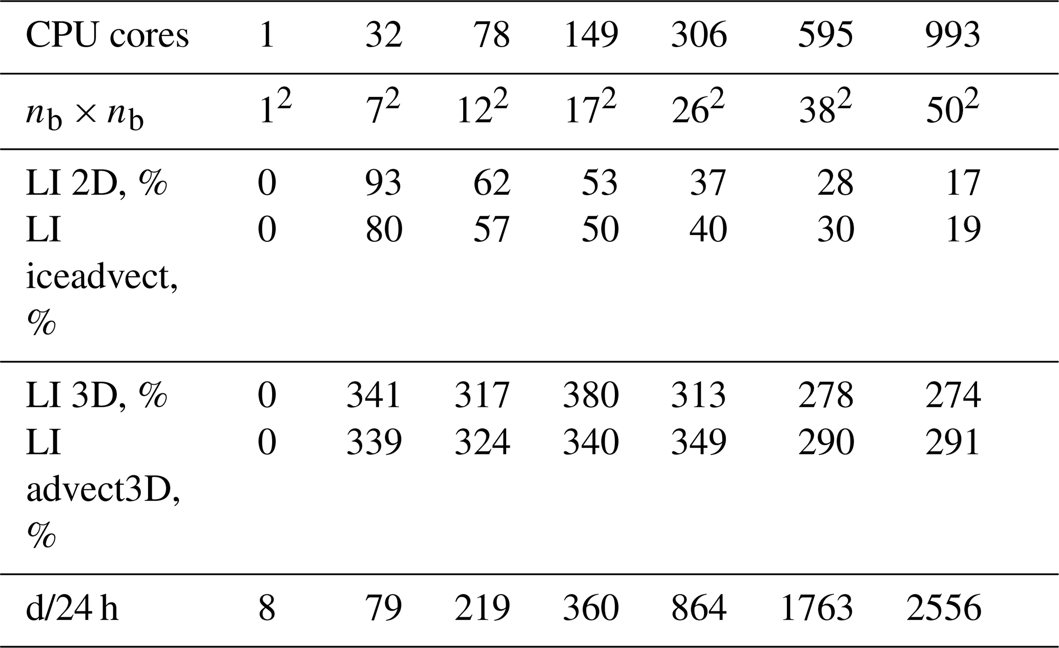
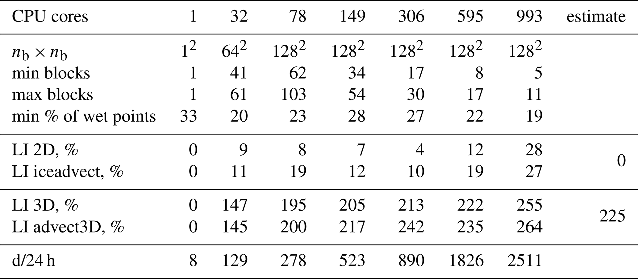
Table 1 The model with the 1block partition: n_b×n_b is the grid of blocks, and LI 2D and LI 3D are load imbalances (Eq. 3) for weights w_2d and w_3d, respectively. “LI iceadvect” and “LI advect3D” are LIs computed based on the runtime of corresponding functions without exchanges, and d/24 h is the number of computed days for 1 astronomical day.

4 Organization of the calculations in non-parallel code

Computations in the ocean and sea-ice components are performed using three-dimensional arrays, such as $a(i,j,k)$ or $b(i,j,m)$, where i and j represent the horizontal grid indices, k represents the depth layer, and m represents the ice gradation. The differential operators are local: only neighboring grid nodes – that is, $a(i\pm \mathrm{1},j\pm \mathrm{1},k)$ – are used.

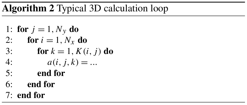
Typical differential operators in the ocean component are organized as shown in Algorithm 2, where N_x=500, N_y=500, and K(i,j) represents the number of depth layers. For land points, $K(i,j)=\mathrm{0}$ and $K(i,j)\in [\mathrm{3},\mathrm{39}]$, with an approximate mean value of 12 for the remaining wet points; see Fig. 1.

Differential operators in the ice component are shown in Algorithm 3, where M=14 or 15 is the number of ice gradations, and mask(i,j) is the logical mask of wet points. The percentage of wet points is 33 %.

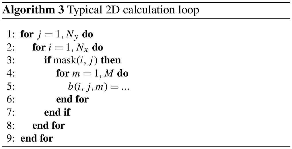
Note that arrays in Fortran are arranged in column major order, so the first index i is linear in memory. The presented arrangement of indices is common for ocean models (see, for example, NEMO documentation; Madec et al., 2008). The loop arrangement is utilized from the original code. Although another arrangement may be more efficient, it does not affect the parallelization approach given later on. In spite of the fact that the inner loop does not have stride-1 access, we can speculate that it allows for possible automatic vectorization over the m index and corresponds to minimal control-flow interruptions due to false mask(i,j) values.

5 Modifications of the non-parallel code

In this section we describe the partitioning algorithm of the model domain into subdomains, each corresponding to a CPU core, and subsequent modifications of the single-core calculations, which require only minor changes to Algorithms 2 and 3. Grid partition is performed in two steps: the model domain is decomposed into small blocks, and then these blocks are distributed over CPU cores in such a way that computational load imbalance is minimized. We utilize a common grid partition for both sea-ice and ocean submodels and provide theoretical estimates of the load imbalances resulting from the application of different weight functions in the balancing problem. The partition is calculated during the model initialization stage, as our balancing algorithm (Hilbert curves) is computationally inexpensive. Also, we guarantee that the partition is the same each time the model is run if the parameters of the partitioner were not modified.

Computational domain $[\mathrm{1},N_x]\times [\mathrm{1},N_y]$ is separated into n_b×n_b blocks. If integer division is impossible, then block sizes are $n_x(i_{\mathrm{b}},j_{\mathrm{b}})=N_x\text{div}{n}_{\mathrm{b}}$ and $n_y(i_{\mathrm{b}},j_{\mathrm{b}})=N_y\text{div}{n}_{\mathrm{b}}$, where $i_{\mathrm{b}},j_{\mathrm{b}}\in [\mathrm{1},n_{\mathrm{b}}]$ represents horizontal indices of the blocks. The other points are distributed over the first blocks: n_x(i_b,j_b)1, where $i_{\mathrm{b}}\in [\mathrm{1},N_x\text{mod}{n}_{\mathrm{b}}]$ and $j_{\mathrm{b}}\in [\mathrm{1},n_{\mathrm{b}}]$; and n_y(i_b,j_b)1, where $i_{\mathrm{b}}\in [\mathrm{1},n_{\mathrm{b}}]$ and $j_{\mathrm{b}}\in [\mathrm{1},N_y\text{mod}{n}_{\mathrm{b}}]$. The set of indices corresponding to a block is denoted by $\mathrm{\Omega }(i_{\mathrm{b}},j_{\mathrm{b}})=\left[i_{\mathrm{s}}\right(i_{\mathrm{b}},j_{\mathrm{b}}),i_{\mathrm{e}}(i_{\mathrm{b}},j_{\mathrm{b}}\left)\right]\times \left[j_{\mathrm{s}}\right(i_{\mathrm{b}},j_{\mathrm{b}}),j_{\mathrm{e}}(i_{\mathrm{b}},j_{\mathrm{b}}\left)\right]$.

To formulate a balancing problem, we must assign weights of computational work to each block and then distribute them among N_p available CPU cores in such a way that all cores have the same amount of work to do, or we must come as close to this as possible provided that the “quality” of the partition is kept. Connectivity of subdomains (by subdomain we refer to a set of blocks belonging to a CPU core) or the minimum length of the boundary can be chosen as possible criteria for the quality of a partition. The weight for a block is the sum of weights corresponding to grid points in the range Ω(i_b,j_b). The following weights are chosen for 2D and 3D computations, respectively:

$$\begin{array}{}\text{(1)}& {\displaystyle }& {\displaystyle }{w}_{\text{2d}}(i,j)=\text{mask}(i,j),\text{(2)}& {\displaystyle }& {\displaystyle }{w}_{\text{3d}}(i,j)=K(i,j)/\text{mean}\left(K\right),\end{array}$$

where the “mean” operation is applied over wet points.

5.1 Trivial 1block partition

For a fixed n_b, one can find the number of wet blocks (i.e., blocks with at least one non-land point). In this partition, the number of cores N_p is equal to the number of wet blocks, and each CPU core gets exactly one block; see Fig. 2. By varying n_b, possible values of N_p can be found.

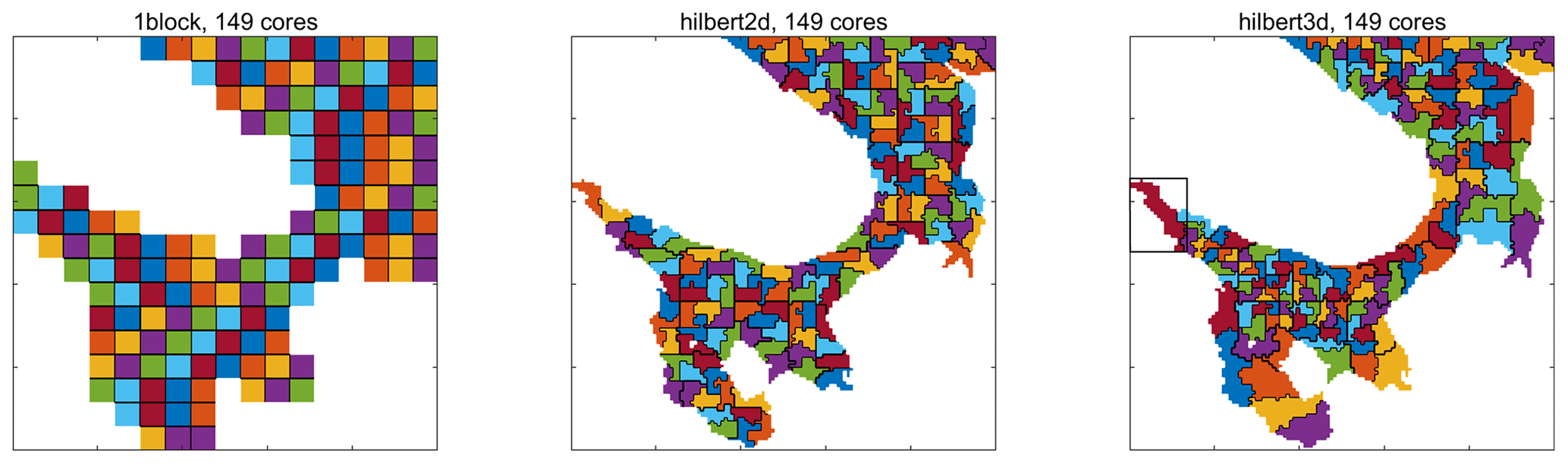
Figure 2 Three types of partition. Different processor cores are separated by a black line. Hilbert partitions are based on a grid of $n_{\mathrm{b}}\times n_{\mathrm{b}}=\mathrm{128}\times \mathrm{128}$ blocks. Colors can repeat. The black rectangle in the figure for the hilbert3d partition corresponds to a “shared” array allocated for blocks belonging to a given CPU core.

5.2 Hilbert-curve partition

For n_b being a power of 2, the Hilbert curve connecting all the blocks can be constructed (Bader, 2012). This gives a one-dimensional set of weights that is balanced using the simplest algorithm. The sum of the block weights on the p core is denoted by W_p. In spite of the fact that the Hilbert curve possesses the locality property (i.e., close indices on the curve correspond to close indices on the grid), it may not provide a partition into connected subdomains if there are a lot of land blocks. To overcome the problem of possible loss of connectivity, we perform the following optimization procedure; see Algorithm 4.

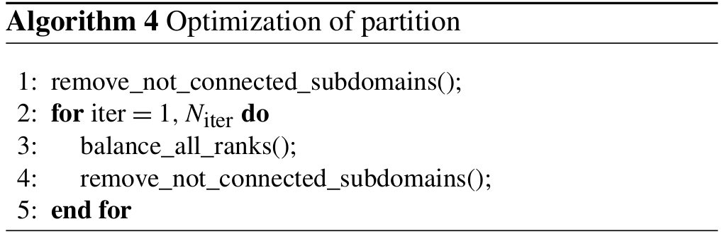
Function remove_not_connected_subdomains() finds the connected subdomain with the maximum work for each CPU core and sends other blocks to neighboring cores. Function balance_all_ranks() tries to send bordering blocks for each core to neighboring cores to minimize the maximum work on both cores: $max(W_p,W_{p^{\prime }})\to min$, where W_p and $W_{p^{\prime }}$ are for the work on the current CPU core and on a neighboring core, respectively. The number of iterations is user-defined, and we choose N_iter=15, which is usually enough to reach convergence. Note that optimization does not guarantee a global optimum, and function remove_not_connected_subdomains() may increase load imbalance. Thus, we choose the iteration with the best balancing. The need for partitioning into connected subdomains comes from the intention to increase the percentage of wet points on CPU cores due to the data structure used; see the following section for a definition of the shared array.

The described algorithm performs partitioning into connected subdomains with load imbalance, which is

$$\begin{array}{}\text{(3)}& \text{LI}=\mathrm{100}\mathit{\%}\cdot {\displaystyle \frac{max\left(W_p\right)-\text{mean}\left(W_p\right)}{\text{mean}\left(W_p\right)}},p\in [\mathrm{1},N_p],\end{array}$$

representing no more than 10 % in most cases. This is an acceptable accuracy because partitioning itself is not the main objective of the article.

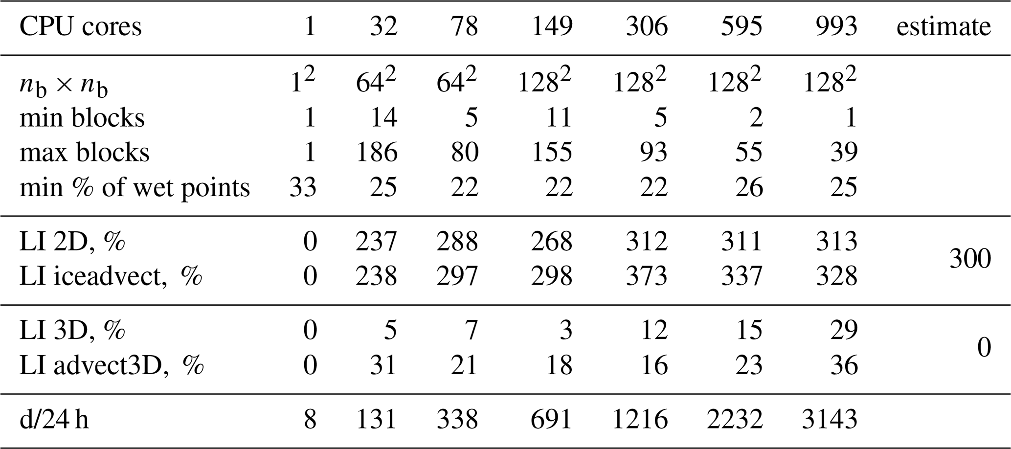
We have implemented two baseline partitions: hilbert2d (with weights w_2d) and hilbert3d (with weights w_3d); see Fig. 2. As one can see, hilbert2d divides the computational domain on quasi-uniform subdomains, while hilbert3d locates many CPU cores in high-depth regions and few cores in shallow water. The minimum and maximum number of blocks on a core can be found in Tables 2 and 3. When one of these partitions is applied to the whole coupled ocean–ice model, it balances one submodel and unbalances another. Table 2 shows that balancing of 2D computations ($\text{LI 2D}\to min$) leads to an imbalance in 3D computations (LI 3D≈200 %), and Table 3 shows the opposite behavior with LI 2D≈300 %. These values are close to the estimates given in Appendix A and defined by the ratio between the minimum, maximum, and mean integer depth. The presented LI values imply a slowdown of one of the submodels by 3 to 4 times because LI increases runtime (T) compared to the optimal one (T_opt) in the following way:

$$\begin{array}{}\text{(4)}& T=(\text{LI}+\mathrm{1})T_{\text{opt}}.\end{array}$$

Table 2 Same as Table 1, but for the hilbert2d partition; min and max operations are applied over CPU cores. The column “estimate” shows the theoretical LI values given in Appendix A.

Table 3 Same as Table 2, but for the hilbert3d partition.

A compromise for both submodels can be found by considering a combination of weights:

$$\begin{array}{}\text{(5)}& w_{\text{2d3d}}=w_{\text{2d}}+{\mathit{\gamma }}_{\mathrm{0}}{w}_{\text{3d}},\end{array}$$

where γ₀≈3 is a ratio of runtimes for ocean and ice submodels on one CPU core. A partition of this type is denoted by hilbert2d3d. While this weight is optimal for “overlapping” computations of two code sections with different complexity, it is also the optimal weight for “non-overlapping” code sections (i.e., separated by blocking MPI exchanges). We show this in Appendix B with corresponding estimates of LI for 2D (130 %) and 3D (34 %) computations.

5.3 Data structure and MPI exchanges

After partitioning has been performed, we get a set of blocks for each CPU core p, $I_p=\mathit{\left\{}\right(i_{\mathrm{b}},j_{\mathrm{b}}\left)\mathit{\right\}}$. Shared data arrays are allocated for all blocks belonging to a CPU core with the following range of indices (excluding halo):

$$\begin{array}{}\text{(6)}& {\displaystyle }& {\displaystyle }{i}_{\mathrm{s}}^p=min\left(i_{\mathrm{s}}\right(I_p\left)\right),i_{\mathrm{e}}^p=max\left(i_{\mathrm{e}}\right(I_p\left)\right),\text{(7)}& {\displaystyle }& {\displaystyle }{j}_{\mathrm{s}}^p=min\left(j_{\mathrm{s}}\right(I_p\left)\right),j_{\mathrm{e}}^p=max\left(j_{\mathrm{e}}\right(I_p\left)\right),\text{(8)}& {\displaystyle }& {\displaystyle }a(i_{\mathrm{s}}^p:i_{\mathrm{e}}^p,j_{\mathrm{s}}^p:j_{\mathrm{e}}^p,:).\end{array}$$

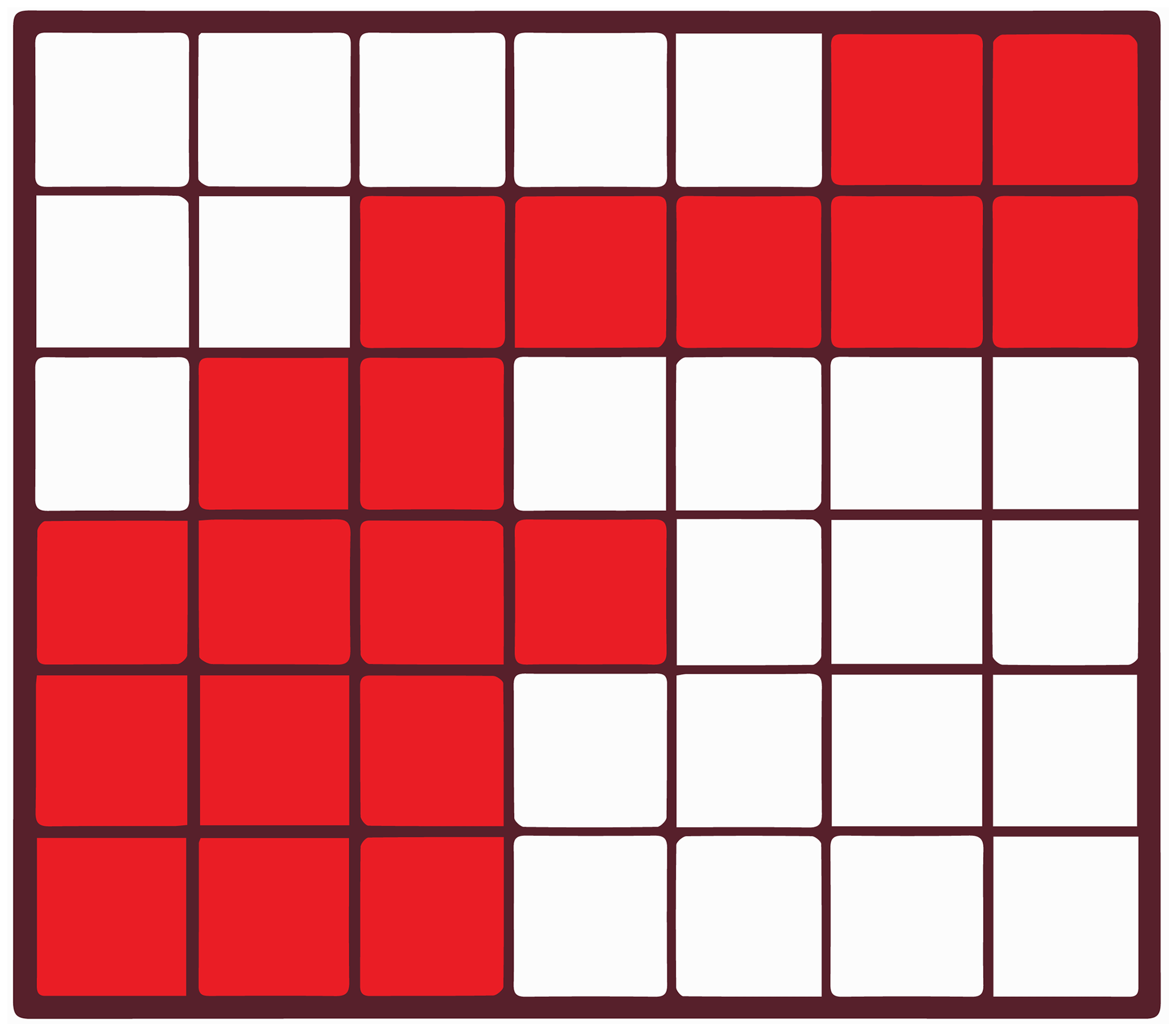
Figure 3 Blocks belonging to a CPU core are in color, and borders of the allocated array are indicated by a thick line; ${\text{mask}}_p(i,j)=\mathrm{1}$ in colored blocks and 0 elsewhere.

An example of the shared array size is shown by the rectangle in Fig. 2 for a particular CPU core. We introduce a mask of grid points belonging to a CPU core (mask_p(i,j)). Correspondence between blocks, the shared array, and the mask is clarified in Fig. 3. Introducing this mask does not increase the complexity of the algorithms because the mask of the wet points already exists in the original code and is simply modified. Finally, only minor modifications of the original loops are necessary:

$$\begin{array}{}\text{(9)}& {\displaystyle }& {\displaystyle }\mathrm{1},N_x\to i_{\mathrm{s}}^p,i_{\mathrm{e}}^p,\text{(10)}& {\displaystyle }& {\displaystyle }\mathrm{1},N_y\to j_{\mathrm{s}}^p,j_{\mathrm{e}}^p,\text{(11)}& {\displaystyle }& {\displaystyle }K(i,j)\to K(i,j)\cdot {\text{mask}}_p(i,j),\text{(12)}& {\displaystyle }& {\displaystyle }\text{mask}(i,j)\to \text{mask}(i,j)\cdot {\text{mask}}_p(i,j).\end{array}$$

Table 4 Same as Table 2, but for the hilbert2d3d partition; “estimate” is given in Appendix B.

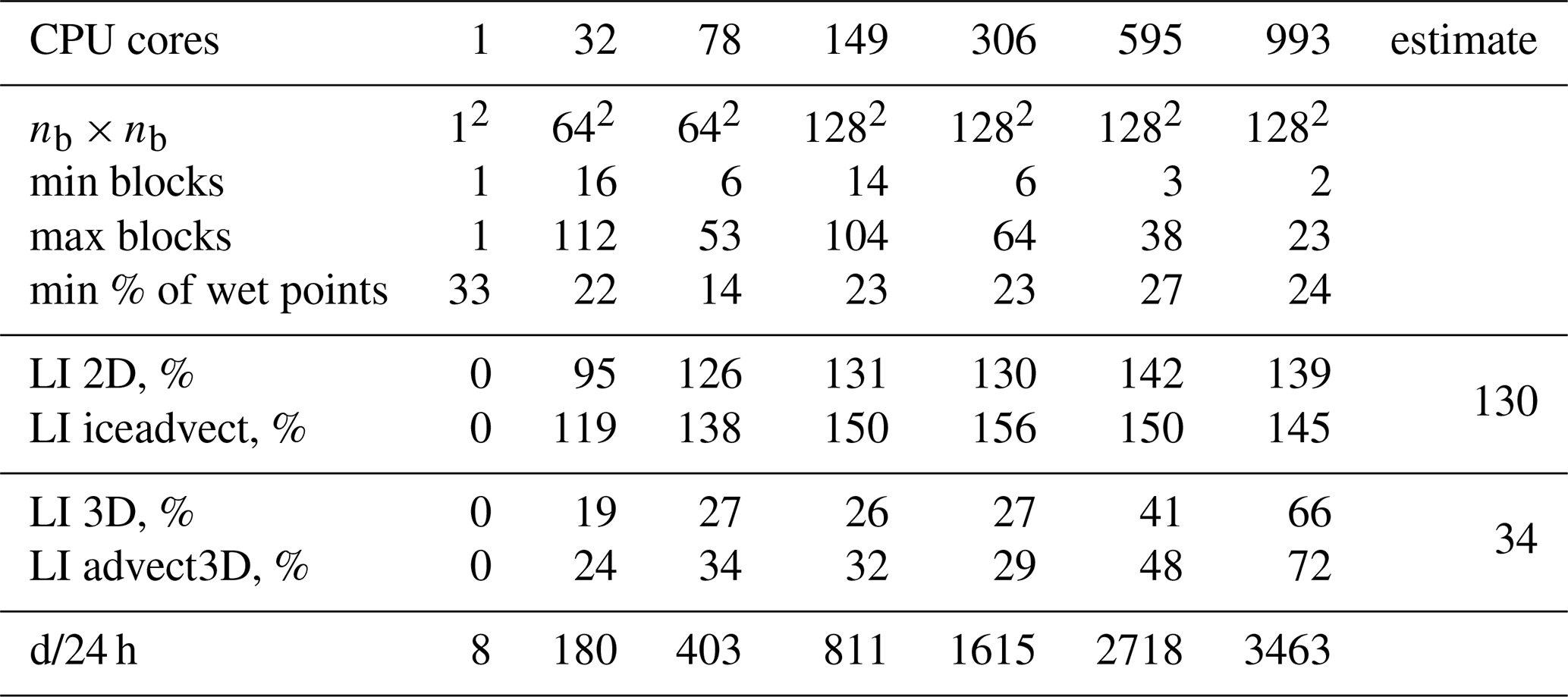
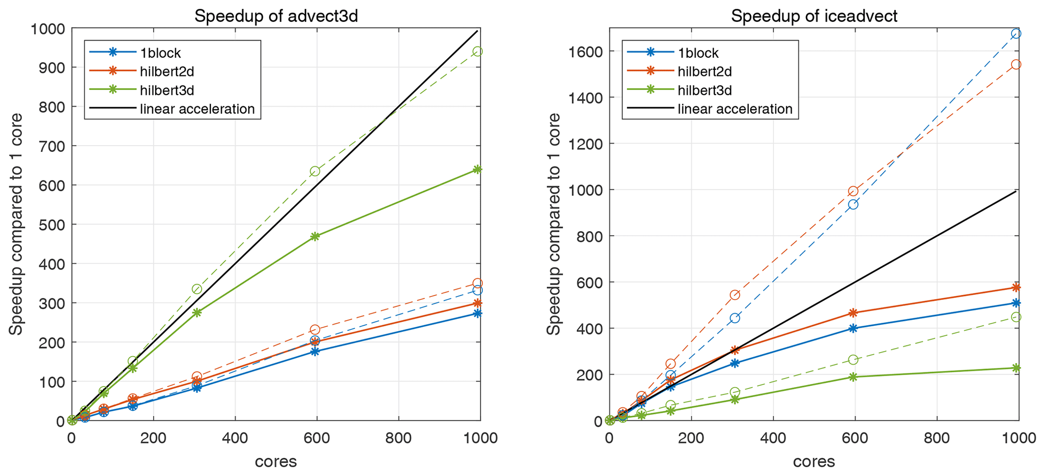
Figure 4 Speedup compared to one core for two functions: advect3D and iceadvect. Solid and dashed lines correspond to measurements with and without MPI exchanges, respectively. Different partitions are shown in color (1block, hilbert2d, and hilbert3d).

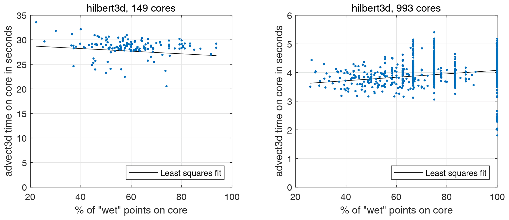
Figure 5 Scatter plot: percentage of wet points on a core – advect3D runtime (without MPI exchanges for 1 model day). Each point corresponds to one CPU core. Figures correspond to the hilbert3d partition with different numbers of CPU cores.

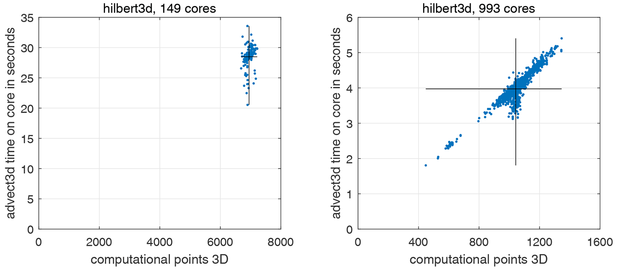
Figure 6 Scatter plot: number of computational points for 3D calculations on a core – advect3D runtime (without MPI exchanges for 1 model day). Each point corresponds to one CPU core. Solid lines show the average values along the x and y axes. Figures correspond to the hilbert3d partition with different numbers of CPU cores.

Usually (see Dennis, 2007, 2003), arrays are allocated for each block separately. This has the following advantages.

• There is more efficient cache usage.

• If the number of blocks is large enough to get proper balancing, then there is no need for mask_p(i,j), thus giving an advance in vectorization and so on.

It also introduces some drawbacks.

• There are overheads for copying block boundaries (small blocks like 4×4 are prohibited).

• Many modifications of the original code are necessary, especially in service routines, I/O, and so on.

Consequently, the main strength of our approach is the ability to incorporate balancing while keeping the original program code as simple as for the trivial 1block partition. We expect that a shared array may be not optimal for near-land CPU cores with ≈20 % wet points because of non-efficient cache usage. An example of such a core is shown by the rectangle in Fig. 2. An experimental study of runtime dependence on the percentage of wet points will be carried out.

Borders of blocks neighboring other CPU cores are sent using MPI. The following optimizations are applied to reduce the exchange time.

• All block boundaries adjacent to a given CPU core are copied to a single buffer array, which is sent in one MPI_Send call.

• If possible, a diagonal halo exchange is included in cross-exchanges with extra width.

• There is an option to send borders of two or more model fields in one MPI_Send call.

• Borders in the sea component are sent up to K(i,j) depth (i.e., only the actually used layers are transmitted).

The first three points reduce the latency cost in many cores, and the final point reduces bandwidth limitations.

5.4 Parallel solver of the SLAE

As we have already mentioned, the time-implicit equation for the free surface is reduced to an SLAE with a sparse 19-diagonal matrix. This is solved by a parallel implementation of the BICGSTAB algorithm preconditioned by block ILU(0) with overlapping blocks; see Saad (2003). The ILU(0) preconditioner preserves the 19-diagonal matrix structure, wherein matrix blocks are defined for each CPU core and correspond to wet points plus a band of border points of width 2. Because blocks are defined by the partition, the convergence rate depends on the number of CPU cores. Nevertheless, we have found that in the range from 1 to 996 CPU cores, it is sufficient to perform 6 to 10 iterations in order to reach the relative residual $\Vert Ax-b\Vert /\Vert b\Vert \le {\mathrm{10}}^{-\mathrm{6}}$.

6 Numerical experiments

Our experiments were performed on the cluster at the Joint Supercomputer Center of the Russian Academy of Sciences (http://www.jscc.ru/, last access: 2 February 2021). Each node includes two 16-core Intel Xeon E5-2697Av4 processors (Broadwell). The software code was compiled by the Intel Fortran Compiler ifort 14.0.1 with the optimization option -O2. Low-core simulations were performed for 3 model days (2592 time steps). The model on 993 CPU cores is launched for 30 d, with subsequent rescaling of the results. During the first day, we call an MPI_Barrier function to measure the performance of particular procedures with and without exchanges. During the last 2 d, an MPI_Barrier is omitted and overall performance is assessed. The number of cores for tests is guided by the 1block partition method, which is highly restricted in the allowable number of cores. We first show how the most time-consuming functions corresponding to ocean and ice submodels accelerate for three partitions: 1block, hilbert2d, and hilbert3d (see Fig. 2). We then study the overall performance of the model using four partitions, including hilbert2d3d with combined weights (Eq. 5).

The maximum grid size of blocks for our model is $n_{\mathrm{b}}\times n_{\mathrm{b}}=\mathrm{128}\times \mathrm{128}$ because the MPI exchange width is limited by the block size, while the SLAE solver requires an exchange of width 2. Note that due to the data structure that we used, the performance of Hilbert-type partitions is almost insensitive to n_b at a moderate number of CPU cores. Nevertheless, n_b may be tuned by hand to decrease the complexity of the partition optimization procedure or to increase the percentage of wet points on a core. In runs with many CPU cores, we use the maximum available number of blocks to get better balancing. The parameters that we used in the experiments are given in Tables 1, 2, 3, and 4.

6.1 Speedup of scalar and ice advection

Advections of scalars (advect3D, depth-dependent) and ice (iceadvect, depth-independent) are the most time-consuming procedures in ocean and ice submodels, respectively. In the following, we will show that the hilbert3d partition is appropriate for advect3D and hilbert2d for iceadvect.

Speedup for the mentioned procedures is given in Fig. 4. Dashed lines correspond to measurements of code sections between MPI exchanges and show how pure computations accelerate. Pure computations in advect3D accelerate linearly for the hilbert3d partition, while pure computations in iceadvect accelerate superlinearly for the hilbert2d partition. Superlinearity (parallel efficiency is greater than 100 % when “doubling” the number of cores) occurs in the range of cores 1–149, and we have investigated the possible reasons for this using the open-access Intel Advisor profiler. We have found that on 1 core the most time-demanding memory requests are the DRAM data upload, while on 149 cores most memory requests correspond to the L1 cache. Thus, superlinearity can be partially explained by better cache utilization when the number of cores increases. Note that more local memory access pattern (MAP) can decrease the limitations caused by the memory requests and can be achieved by incorporating stride-1 access for the inner loop indices, but we leave this point for optimizations in the future.

Speedup including MPI exchanges is shown in Fig. 4 with solid lines. The function advect3D is only slightly limited by MPI exchanges on 993 cores: its speedup on the partition hilbert3d falls from 940 to 640 when exchanges are accounted for. Meanwhile, iceadvect loses speedup from 1540 to 576 after accounting for exchanges on the hilbert2d partition. Both functions have an identical number of exchanges, but advect3D is more computationally expensive. Consequently, we explain the worse performance of iceadvect by a lower ratio of the number of operations to the number of points to exchange. A similar bottleneck due to exchanges in 2D dynamics is reported in Koldunov et al. (2019a). The hilbert2d partition has a slight advantage (about 15 %–20 %) over the 1block partition for both functions (see solid lines). In total, as we expected, the hilbert3d partition is suitable for the advect3D function, and its acceleration is 2 to 3 times more efficient than when the 1block and hilbert2d partitions are used. Also, the hilbert2d and 1block partitions show the function iceadvect that is 2 to 4 times faster compared to the hilbert3d partition. The different accelerations are strongly connected to balancing of computations. To check partition-based (LI 3D and LI 2D) and runtime-based (LI advect3D and LI iceadvect, respectively) load imbalance for 3D and 2D computations, see Tables 1–3. Note that theoretical and practical LIs are moderately close to each other, which confirms our choice of weights (Eqs. 1 and 2) for these functions. Also note that the data structure and organization of the calculations are appropriate for load balancing.

Figure 7 Speedup compared to one core for the full model. Different partitions are shown in color (1block, hilbert2d, hilbert3d, hilbert2d3d).

Figure 8 Relative contribution of different code sections to runtime; ocean – all procedures corresponding to ocean submodel including advect3D, ice – ice submodel including iceadvect, processing – computation of statistics, I/O – input/output with scatter–gather functions, SLAE – matrix inverse, other – simple service procedures.

Further analysis reveals that the runtime-based LI could be 4 %–25 % more than the partition-based one; see Tables 2 and 3. This may be connected to overheads introduced by non-efficient organization of memory. We allocate a shared array for all blocks belonging to a CPU core, and near-land cores may have only 20 % of the wet points (see Tables 2 and 3), which can lead to an increase in cache misses. Figure 5 shows a scatter plot for the percent of wet points vs. advect3D runtime without exchanges (each point corresponds to some CPU core). One can clearly see that on a moderate number of cores (149) the computations are limited by the core with the smallest percentage of wet points, which has the maximal runtime. Figure 6 additionally shows that the spread in runtime cannot be explained by the difference in the number of computational points; i.e., the partitioning algorithm works well for 149 cores. Although organization of the calculations may slightly limit model efficiency on a moderate number of cores, it does not limit the model efficiency on 993 cores, for which the major part of the advect3D runtime spread is explained by the imperfect balancing (see Fig. 6) but not the data structure (see Fig. 5). Stagnation of the balancing procedure is evident from the fact that the minimum number of blocks located on a CPU core is 1 for 993 cores; see Table 3. Note that the computational subdomain corresponding to one CPU core is small enough: on average, it has 9×9 horizontal points with 12 vertical levels for 993 cores.

6.2 Speedup of the full model

The coupled ocean–ice model is launched on the same CPU cores for both submodels with a common horizontal partition. Input/output functions are sequential and utilize gather–scatter operations, which are given by our library of parallel exchanges. Speedup for the full model compared to one CPU core is given in Fig. 7. Maximum speedup, approximately 430, corresponds to the partition with combined weights (hilbert2d3d) on 993 cores. Compared to the simplest partition (1block), the hilbert2d3d model is 115 % faster on 149 cores and 40 % faster on 993 cores. Partition hilbert2d3d also gives an advantage over partitions balancing purely 2D and 3D computations (hilbert2d, hilbert3d). On 993 CPU cores, the parallel exchanges in this model have the following contributions to the runtime: 20 % for boundary exchanges, 18 % for gather–scatter, and 6.5 % for Allreduce.

The relative contribution of different code sections to runtime is given in Fig. 8. In the case of perfect scaling of all procedures, the relative contribution must be the same as the number of CPU core rises. For partitions 1block and hilbert2d, we see a slowdown of the ocean component. Partition hilbert3d suffers from a slowdown of the ice component. Finally, the closest preservation of time distribution is found for the hilbert2d3d model. We did not pay much attention to the processing code section because, although it accelerates, its computational cost could be reduced. The section I/O gradually saturates due to gather–scatter operations, which consume 85 % of I/O runtime on 993 CPU cores. The new parallel solver (SLAE) has fast convergence and low computational cost but suffers from Allreduce operations: in our implementation each iteration demands five MPI_Allreduce calls, which account for 60 % of SLAE code section runtime on 993 cores.

Figure 9 Absolute contribution of different code sections to runtime on 993 CPU cores.

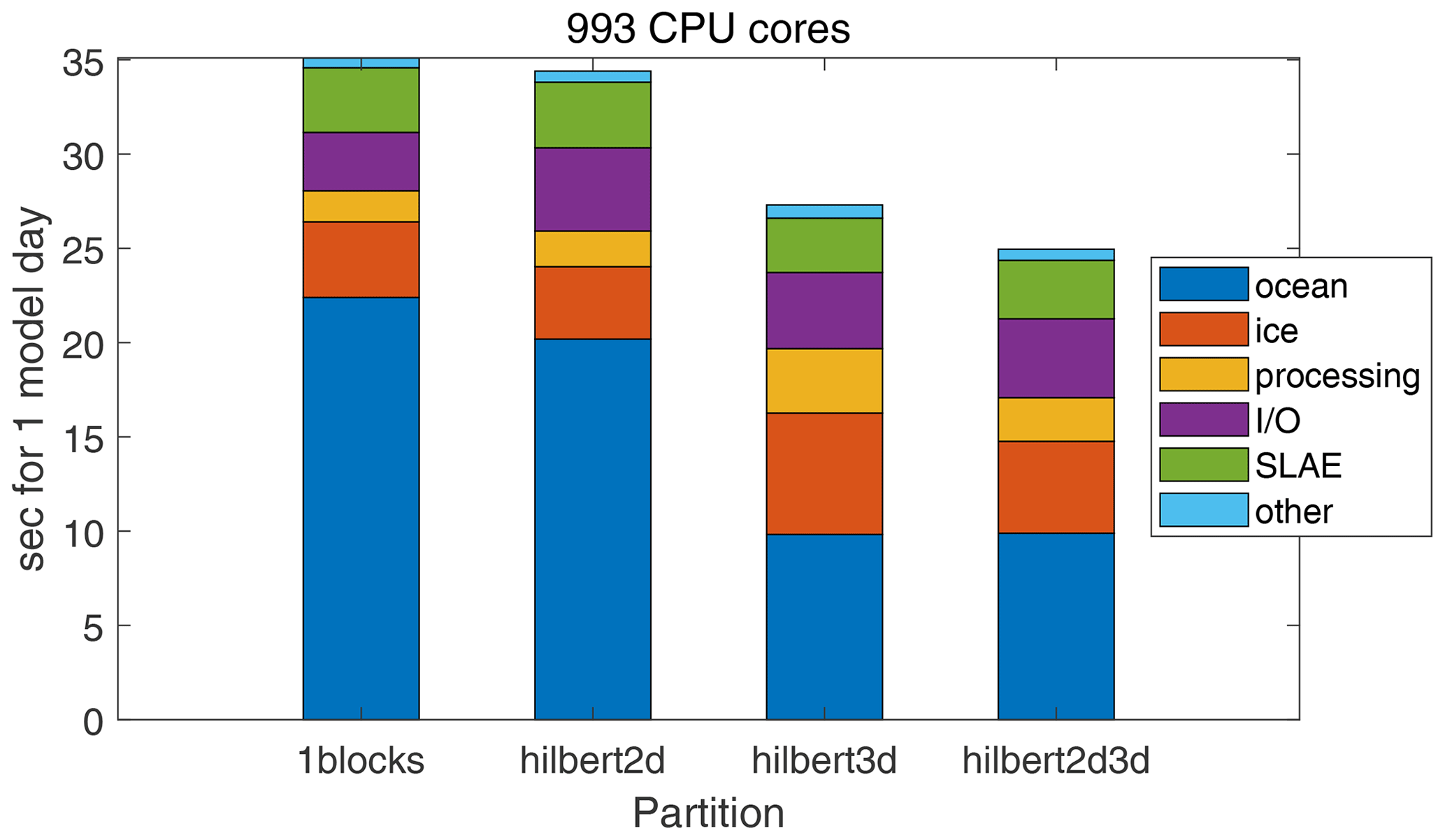
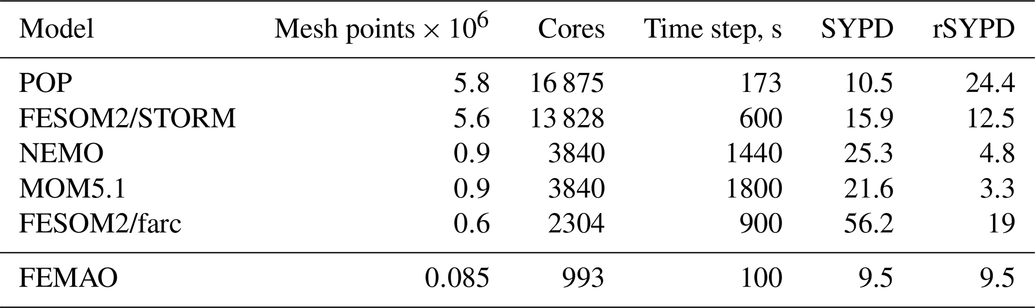
Table 5 Efficiency of the time step loop for the FEMAO model compared to global ocean–ice models. Rescaled SYPD (rSYPD, Eq. 13) accounts for the difference in time steps and the number of horizontal mesh points and CPU cores. Original values are published in Koldunov et al. (2019a), Huang et al. (2016), and Ward (2016), but we took our values directly from Table 3 in Koldunov et al. (2019a).

Absolute values of code section runtimes for 1 model day are shown in Fig. 9. In comparison to the hilbert3d partition, combining of weights (hilbert2d3d) reduces the cost of the ice component while keeping the ocean component almost without changes (see also Tables 3 and 4 for load imbalance values). In addition, the processing section reduces its runtime because it contains many service functions that are not fully optimized and that are sensitive to stretching of the horizontal area covered by a CPU core: such stretching is done by the hilbert3d partitioner.

Simulated years per wall-clock day (SYPD) for the best configuration (hilbert2d3d, 993 cores) are calculated as $\mathrm{3463}/\mathrm{365}\approx \mathrm{9.5}$; see Table 4. A direct comparison with other coupled ocean–ice models cannot be achieved because our configuration is rare. However, we can rescale the performance (rSYPD) of the time step efficiency of the global models in the following way:

$$\begin{array}{}\text{(13)}& \text{rSYPD}=\text{SYPD}{\displaystyle \frac{N_{\text{mesh}}}{N_{\text{mesh}}^{\text{FEMAO}}}}{\displaystyle \frac{\mathrm{\Delta }{t}^{\text{FEMAO}}}{\mathrm{\Delta }t}}{\displaystyle \frac{N_p^{\text{FEMAO}}}{N_p}},\end{array}$$

where we take into consideration different numbers of horizontal mesh wet points (N_mesh), different numbers of CPU cores (N_p), and different time steps (Δt), but we neglect different numbers of vertical levels and differences in the formulation of the ice dynamics. As follows from Table 5, rSYPD is of the order of 10 for all of the ocean–ice models that we have presented, including FEMAO. While this characteristic cannot rate models by their efficiency, we argue that our parallel configuration is comparable to existing parallel ocean–ice models.

7 Conclusions

In this paper, we present a relatively simple approach to accelerate the FEMAO ocean–ice model based on a rectangular structured grid with advances in load balancing. The modifications that had to be introduced into the program code are identical to those that were required by the simplest decomposition on squares. The only demand on the model to be accelerated by this technique is marking computational points by a logical mask. In the first step, we utilize the common partition for ocean and ice submodels. For a relatively “small” model configuration of 500×500 horizontal points, we reach parallel efficiency of 60 % for particular functions (3D scalar advection using the 3D-balancing approach and 2D ice advection using the 2D-balancing approach) and 43 % for the full model (using the combined weight approach) on 993 CPU cores. We show that balancing the 3D computations leads to unbalanced 2D computations and vice versa. Consequently, further acceleration may be achieved by performing computations of 2D and 3D components on distinct groups of CPU cores with different partitions. Nevertheless, high parallel efficiency of 3D scalar advection itself is a great advance for future applications of the model, especially for the version with a pelagic ecology submodel (Chernov et al., 2018), wherein more than 50 3D scalars (biogeochemical concentrations) are added to the thermohaline fields.

Note that while the parallel approach that we have presented here can be implemented into the model in a relatively simple way, the code of the library of parallel exchanges can be rather complex (see the “Code availability” section).

Appendix A: Estimating the load imbalance for hilbert2d and hilbert3d partitions

Let us introduce two functions of bathymetry (defined by integer depth K(i,j)) with the corresponding values for our model:

$$\begin{array}{}\text{(A1)}& {\displaystyle }& {\displaystyle }{\mathit{\rho }}_{max}\left(K\right)={\displaystyle \frac{max\left(K\right)}{\text{mean}\left(K\right)}}={\displaystyle \frac{\mathrm{39}}{\mathrm{12}}}=\mathrm{3.25},\text{(A2)}& {\displaystyle }& {\displaystyle }{\mathit{\rho }}_{min}\left(K\right)={\displaystyle \frac{\text{mean}\left(K\right)}{min\left(K\right)}}={\displaystyle \frac{\mathrm{12}}{\mathrm{3}}}=\mathrm{4},\end{array}$$

here and below, “mean”, “min”, and “max” operations correspond only to wet points. These values define how balancing of 2D computations affects 3D computation imbalance and vice versa. Let S and V be sets of surface and ocean points, respectively, S_p and V_p be sets of these points belonging to a CPU core p, and $|\cdot |$ be the number of points in a set. The number of 3D points can be expressed via 2D points:

$$\left|V\right|=\sum _{\mathit{\{}i,j\mathit{\}}\in S}K(i,j)=\left|S\right|\cdot {\text{mean}}_{\mathit{\{}i,j\mathit{\}}\in S}K(i,j).$$

When balancing of 2D computations is used (hilbert2d), surface points are distributed among processors in roughly equal amounts ($\left|S_p\right|=\left|S\right|/N_p$). Then, for 3D computations, the ratio of maximum work to mean work among cores is defined as

$$\begin{array}{ll}\text{(A3)}& {\displaystyle \frac{W_{\text{max}}}{W_{\text{mean}}}}& {\displaystyle }={\displaystyle \frac{{max}_p\left(\right|V_p\left|\right)}{{\text{mean}}_p\left(\right|V_p\left|\right)}}{\displaystyle }& {\displaystyle }={\displaystyle \frac{{\text{max}}_p\left({\text{mean}}_{\mathit{\{}i,j\mathit{\}}\in S_p}K\right(i,j\left)\right)}{{\text{mean}}_p\left({\text{mean}}_{\mathit{\{}i,j\mathit{\}}\in S_p}K\right(i,j\left)\right)}}\\ {\displaystyle }& {\displaystyle }\approx {\mathit{\rho }}_{max},\end{array}$$

and the corresponding load imbalance is

$$\begin{array}{}\text{(A4)}& \text{LI}={\displaystyle \frac{W_{max}-W_{\text{mean}}}{W_{\text{mean}}}}={\mathit{\rho }}_{max}-\mathrm{1}=\mathrm{225}\mathit{\%}.\end{array}$$

When balancing of 3D computations is used (hilbert3d), ocean points are distributed among processors in roughly equal amounts ($\left|V_p\right|=\left|V\right|/N_p$). Then, for 2D computations, the ratio of maximum work to mean work is defined as

$$\begin{array}{ll}\text{(A5)}& {\displaystyle \frac{W_{max}}{W_{\text{mean}}}}& {\displaystyle }={\displaystyle \frac{{max}_p\left(\right|S_p\left|\right)}{{\text{mean}}_p\left(\right|S_p\left|\right)}}{\displaystyle }& {\displaystyle }={\displaystyle \frac{{max}_p\left(\right|V_p|/{\text{mean}}_{\mathit{\{}i,j\mathit{\}}\in S_p}K(i,j\left)\right)}{{\text{mean}}_p\left(\right|S_p\left|\right)}}\\ {\displaystyle }& {\displaystyle }={\displaystyle \frac{\left|V\right|/\left|S\right|}{{\text{min}}_p\left({\text{mean}}_{\mathit{\{}i,j\mathit{\}}\in S_p}K\right(i,j\left)\right)}}\\ {\displaystyle }& {\displaystyle }\approx {\mathit{\rho }}_{min},\end{array}$$

and the corresponding load imbalance is

$$\begin{array}{}\text{(A6)}& \text{LI}={\displaystyle \frac{W_{max}-W_{\text{mean}}}{W_{\text{mean}}}}={\mathit{\rho }}_{min}-\mathrm{1}=\mathrm{300}\mathit{\%}.\end{array}$$

Appendix B: Finding the optimal weight for non-overlapping 2D and 3D calculations

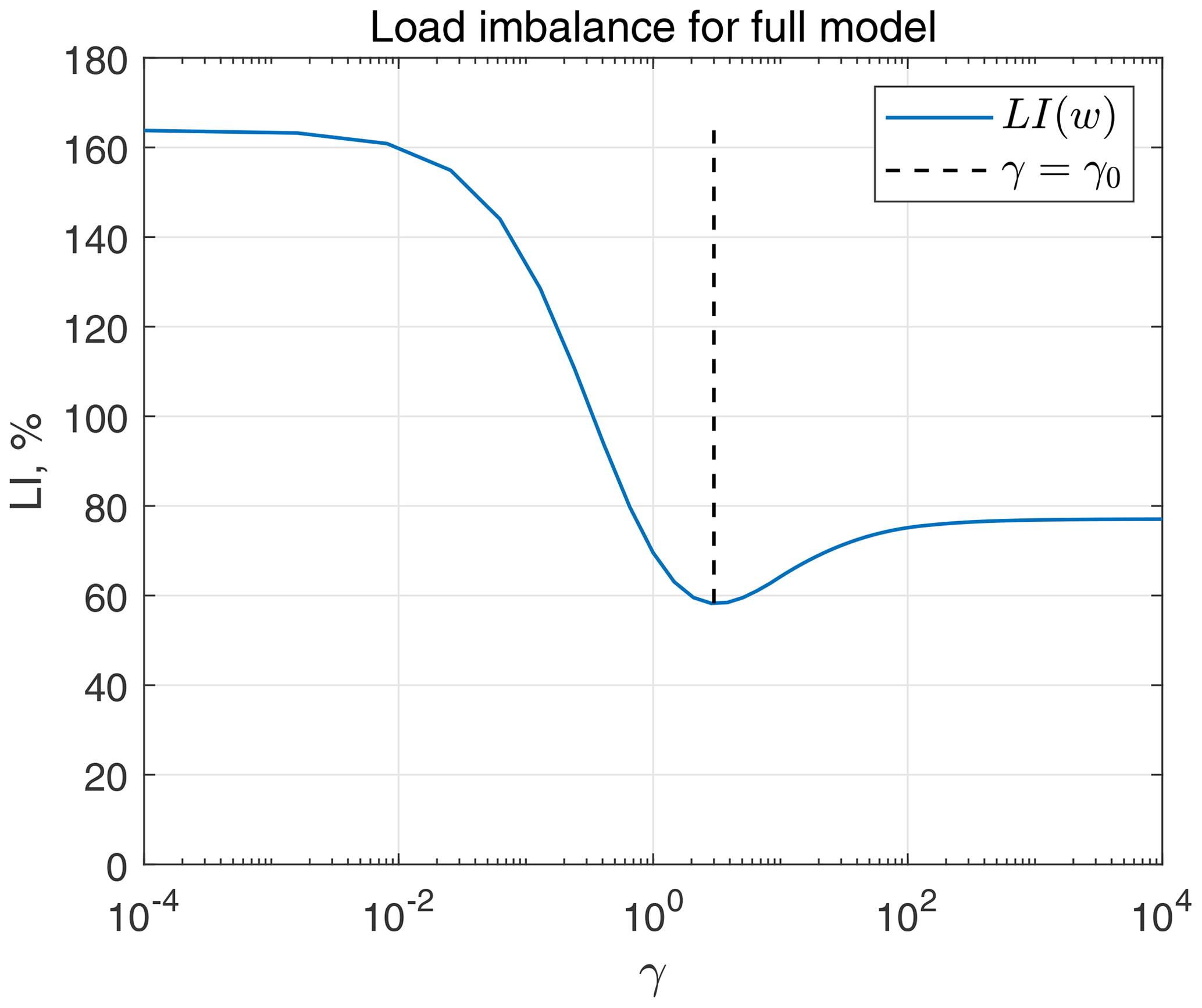
Let W be a full computational work, and let it be distributed between 3D (W^3d) and 2D (W^2d) computations with the ratio γ₀: $W=W^{\text{2d}}+W^{\text{3d}}\sim (\mathrm{1}+{\mathit{\gamma }}_{\mathrm{0}})W^{\text{2d}}$. Our goal is to find a weight function w(i,j), which corresponds to minimal joint (2D and 3D) load imbalance. We use the notation presented in the previous Appendix, and we define the number of computational points corresponding to the weight $\left|V^{\mathrm{w}}\right|={\sum }_{\mathit{\{}i,j\mathit{\}}\in S}w(i,j)$.

Assuming equipartition with respect to this weight ($\left|V_p^{\mathrm{w}}\right|=\left|V^{\mathrm{w}}\right|/N_p$), we can derive LI for 2D calculations,

$$\begin{array}{}\text{(B1)}& {\displaystyle \frac{W_{max}^{\text{2d}}}{W_{\text{mean}}^{\text{2d}}}}={\displaystyle \frac{{max}_p\left|S_p\right|}{{\text{mean}}_p\left|S_p\right|}}\approx {\mathit{\rho }}_{min}\left(w\right),\end{array}$$

and for 3D calculations,

$$\begin{array}{ll}\text{(B2)}& {\displaystyle \frac{W_{max}^{\text{3d}}}{W_{\text{mean}}^{\text{3d}}}}& {\displaystyle }={\displaystyle \frac{{max}_p\left|V_p\right|}{{\text{mean}}_p\left|V_p\right|}}{\displaystyle }& {\displaystyle }={\displaystyle \frac{{max}_p\left(\right|S_p|\cdot {\text{mean}}_{\mathit{\{}i,j\mathit{\}}\in S_p}K(i,j\left)\right)}{{\text{mean}}_p\left(\right|S_p|\cdot {\text{mean}}_{\mathit{\{}i,j\mathit{\}}\in S_p}K(i,j\left)\right)}}\\ {\displaystyle }& {\displaystyle }={\displaystyle \frac{{max}_p\left({\displaystyle \frac{{\text{mean}}_{\mathit{\{}i,j\mathit{\}}\in S_p}K(i,j)}{{\text{mean}}_{\mathit{\{}i,j\mathit{\}}\in S_p}w(i,j)}}\right)}{{\text{mean}}_p\left({\displaystyle \frac{{\text{mean}}_{\mathit{\{}i,j\mathit{\}}\in S_p}K(i,j)}{{\text{mean}}_{\mathit{\{}i,j\mathit{\}}\in S_p}w(i,j)}}\right)}}\\ {\displaystyle }& {\displaystyle }\approx {\mathit{\rho }}_{max}(K/w).\end{array}$$

Finally, assuming that 2D and 3D computations are non-overlapping (i.e., the maximum work is under summation), load imbalance for the full model is calculated as

$$\begin{array}{}\text{(B3)}& \begin{array}{rl}& \text{LI}\left(w\right)={\displaystyle \frac{W_{max}-W_{\text{mean}}}{W_{\text{mean}}}}\\ & ={\displaystyle \frac{{\mathit{\rho }}_{min}\left(w\right)+{\mathit{\gamma }}_{\mathrm{0}}{\mathit{\rho }}_{max}(K/w)}{\mathrm{1}+{\mathit{\gamma }}_{\mathrm{0}}}}-\mathrm{1}.\end{array}\end{array}$$

For a given bathymetry K(i,j), the ratio γ₀=3, and a special type of weight function $w\left(\mathit{\gamma }\right)=w_{\text{2d}}+\mathit{\gamma }{w}_{\text{3d}}$, LI(w(γ)) can be plotted numerically for different values of γ; see Fig. B1. The minimum of this function corresponds to the choice $\mathit{\gamma }={\mathit{\gamma }}_{\mathrm{0}}=\mathrm{3}$, and LI values for 2D and 3D computations in this case are 130 % and 34 %, respectively.

Figure B1 Load imbalance for the full model LI(w(γ)), where $w\left(\mathit{\gamma }\right)=w_{\mathrm{2}\mathrm{d}}+\mathit{\gamma }{w}_{\mathrm{3}\mathrm{d}}$; γ₀=3.