Development of a coupled simulation framework representing the lake and river continuum of mass and energy (TCHOIR v1.0)

Terrestrial surface water temperature is a key variable affecting water quality and energy balance, and thermodynamics and fluid dynamics are tightly coupled in fluvial and lacustrine systems. Streamflow generally plays a role in the horizontal redistribution of heat, and thermal exchange in lakes predominantly occurs in a vertical direction. However, numerical models simulate the water temperature for uncoupled rivers and lakes, and the linkages between them on a global scale remain unclear. In this study, we proposed an integrated modeling framework: Tightly Coupled framework for Hydrology of Open water Interactions in River–lake network (TCHOIR, read as “tee quire”). The objective is to simulate terrestrial fluvial and thermodynamics as a continuum of mass and energy in solid and liquid phases redistributed among rivers and lakes. TCHOIR uses high-resolution geographical information harmonized over fluvial and lacustrine networks. The results have been validated through comparison with in situ observations and satellite-based data products, and the model sensitivity has been tested with multiple meteorological forcing datasets. It was observed that the “coupled” mode outperformed the “river-only” mode in terms of discharge and temperature downstream of lakes; moreover, it was observed that seasonal and interannual variation in lake water levels and temperature are also more reliable in the “coupled” mode. The inclusion of lakes in the coupled model resulted in an increase in river temperatures during winter at midlatitudes and a decrease in temperatures during summer at high latitudes, which reflects the role of lakes as a form of large heat storage. The river–lake coupling framework presented herein provides a basis for further elucidating the role of terrestrial surface water in Earth's energy cycle.

1 Introduction

The temperature of terrestrial surface water plays a vital role in biogeochemical cycles, as it affects the solubility and reactivity of materials and organismal activity (Abril et al., 2014; Ozaki et al., 2003; Webb, 1996). Water temperature can also affect water quality, resulting in adverse impacts on water availability to society. For example, the cooling efficiency of surface water used in power plants and factories is determined by water temperature, and excessively warm return flow sometimes causes thermal pollution downstream of discharge points (Liu et al., 2020; Raptis et al., 2016; van Vliet et al., 2016). A recent study noted that changes in surface water volume and temperature could impact the global heat budget (Vanderkelen et al., 2020). Understanding the thermodynamics of the terrestrial hydrological cycle has become increasingly important for managing freshwater environments and ecosystems, as well as developing global water policies to protect and preserve the Earth's freshwater system.

Some researchers have proposed statistical approaches to describe water temperature, such as correlating water and air temperature and the inertia of water temperature changes (e.g., Keller, 1967; Smith, 1968). Physically based numerical models have also been developed to assess the future impacts of climate change and human activities on water temperature. As rivers and lakes are the major components of terrestrial hydrology, they are governed by extremely different dynamics; hence, different approaches have been adopted for each domain. Previous studies have focused on the role of rivers as horizontal transport pathways for residues from the vertical water balance between the atmosphere and the land surface (Manabe, 1969; Oki et al., 1995). A horizontal one-dimensional model for river water temperature has been developed (e.g., Sinokrot and Stefan, 1993) which assumes that sufficient mixing occurs to ensure that water temperature is uniform in a cross section (Caissie, 2006). In recent years, such a horizontally distributed model has been applied on global scales (e.g., Beek et al., 2012; Tokuda et al., 2019; Wanders et al., 2019) based on the development of global-scale river routing models (e.g., Yamazaki et al., 2011).

Existing studies on the thermal dynamics of lakes have mainly focused on vertical profiles, such as temperature stratification and attenuation of solar radiation (Dake and Harleman, 1969). A breakthrough in model development came through a proposal by Henderson-Sellers (1985) for the parameterization of vertical mixing to bypass explicit calculations of turbulent exchanges by shear stress. This led to the development of several numerical models (e.g., Hostetler and Bartlein, 1990) that solved a diffusion equation with the boundary conditions set at the water surface and lake bottom. These models also assumed that diffusion is primarily driven by density gradients and turbulence, allowing global-scale models to be developed (Stepanenko et al., 2013). In addition to describing the internal dynamics of lakes, lake models have been applied to represent the lower boundary condition of atmospheric models (Dickinson et al., 1993). The impact of lakes on climate at regional scales has been widely studied since the 1990s (e.g., Hostetler et al., 1993; Small et al., 1999). Related models have also estimated that global lake evaporation will be accelerated by changes in surface energy allocation as the climate gets warmer (Wang et al., 2018).

Many modeling efforts do not treat rivers and lakes in an integrated manner. Lake models typically ignore riverine inflow and outflow and describe thermodynamics under the assumption that the elevation of the water surface is constant. For example, a previous study reported a decrease and an increase in the heat capacities of rivers and lakes due to a decrease in water volumes and water temperature warm-up, respectively; however, these models did not properly consider the mass balance of the water budget in reality (Vanderkelen et al., 2020). Another study developed a coupled hydrodynamic and thermodynamic model for rivers and lakes (Bonnet et al., 2000; Yigzaw et al., 2019) and demonstrated that temperature stratification in lacustrine reservoirs affects river temperatures downstream (Li et al., 2015). In particular, Yigzaw et al. (2019) used a continental-scale dataset of river networks that included lakes and reservoirs (hereinafter referred to as “river–lake network”) in the United States. The river–lake networks were constructed by matching lakes with the grids on a river network dataset that previously ignored the presence of lakes and by using the relevant data on the longitude, latitude, and upstream catchment area of each lake. However, although the upstream areas are important for water balance in lakes and reservoirs, it has been reported that this matching method does not work for some reservoirs (Shin et al., 2019). In addition, the latest research developed a river–lake dynamics model for multiple regions by careful integration of river network and lake mask datasets, but a rectangular grid system remains a technical obstacle (Guinaldo et al., 2021).

The research reported herein initially developed a method that enabled the location and shape of lakes to be represented explicitly on a river channel network on a global scale. This technique is an extension of the upscaling method for high-resolution topographic data, representing the shape of a hydrological unit catchment area instead of assuming a rectangular grid system (Yamazaki et al., 2009). It is possible to upscale to any required spatial resolution using this procedure. River and lake sub-models were then coupled to represent the hydrodynamics and thermodynamics of rivers and lakes on the river–lake network dataset created in this study. The modeling framework, called the Tightly Coupled framework for Hydrology of Open water Interactions in River–lake networks (TCHOIR), conserves the mass and energy in rivers and lakes for advection as well as the vertical heat budget. The remainder of this paper is structured as follows: Sect. 2 describes the algorithm used to develop the river–lake network dataset, Sect. 3 presents the development details of the coupling framework and the one-dimensional lake model, Sect. 4 shows the validation results of the river–lake network dataset, Sect. 5 provides the experimental configuration used to validate the framework and the corresponding results, Sect. 6 discusses the effects of thermodynamics of lakes on rivers, Sect. 7 shows the sensitivity test of the validation results of the meteorological forcing datasets, Sect. 8 summarizes the further development of the framework, and Sect. 9 presents the conclusion.

2 Development of the river–lake network dataset

2.1 Harmonization of geographical information

The river–lake network was developed by upscaling high-resolution and global-scale datasets of topographical information, such as MERIT Hydro (Yamazaki et al., 2019), and lake distributions from the HydroLAKES database (Messager et al., 2016). MERIT Hydro derives streamflow direction on a global scale using water body datasets and one of the latest elevation datasets, the MERIT DEM (Yamazaki et al., 2017). It also corrects elevation and streamlines for use in hydrological models and has a spatial resolution of 3 arcsec (∼90 m at the Equator). Moreover, HydroLAKES is used to identify each lake and contains information regarding the spatial shape of lakes and reservoirs (and other attributes, such as name and mean depth of each water body) of more than 1.4 million lakes and reservoirs (in this paper, the term “lake” includes both natural lakes and human-made reservoirs according to the dataset). The shapefile in the HydroLAKES dataset was rasterized to the same spatial resolution as that of MERIT Hydro.

A preliminary analysis showed that the shapes of the lakes registered in HydroLAKES were often larger than the water masks in MERIT Hydro, suggesting that MERIT Hydro underestimates the area of seasonal lakes (e.g., Lake Chad) because the dataset incorporates only permanent water. Our goal for the lake model employed in this study was to represent seasonal or interannual variability of the area of various water surfaces; therefore, lake distribution data were overridden by HydroLAKES instead of using the water distribution data derived from MERIT Hydro.

The merging methods are summarized in Table 1. First, we classified the lakes into two groups according to size: (1) a river–lake network that represents the connectivity of larger lakes with river channels both upstream and downstream (i.e., lakes with an area greater than one upscaled grid area), and (2) smaller lakes treated as sub-grid lakes in a numerical model (i.e., lakes with an area less than one upscaled grid area). For example, in the case of upscaling from the original resolution (i.e., 3 arcsec to 15 arcmin), the minimum lake size in the river–lake network was 90 000 pixels. Consequently, 369 lakes worldwide were represented at the 15 arcmin resolution. We then filled in isolated parts of each lake formed by rasterization of the shapefile (e.g., the rasterized file does not resolve a narrow conduit in Embalse Tucupido Reservoir registered as 880 in HydroLAKES). We then determined the outlet of each lake using flow direction information obtained from MERIT Hydro. When inconsistencies between MERIT Hydro and HydroLAKES created multiple possible outlets for a lake, we selected the outlet with the largest upstream area, following the HydroLAKES algorithm (Messager et al., 2016). In some cases, no outlet for a lake could be found, such as for Lake Balkhash and Large Aral Sea (registered as 12 and 13 in HydroLAKES, respectively). We found that this accurately reflected real-world geography, as both water bodies exist within closed basins. For other endorheic lakes such as the Caspian Sea and Lake Chad, we manually removed incorrectly detected lake outlets. We also adjusted the flow direction for all the grids in each lake to match the outlet location to allow all of the lake grids flow into one river basin if the lake is open. This property changes the size of the river basin if a lake lies between multiple basins on the map, which was upscaled, ignoring the lakes (hereafter called the “river-only” map). Among the 369 lakes resolved at a 15 arcmin resolution, we found 20 lakes lying between multiple basins; of these, 6 lakes are endorheic (e.g., the Caspian Sea and Lake Chad). Most (13) of the other lakes are allocated the basin with the most grids in each lake in the river-only map. Finally, there is only one exception, Laguna Salada (HydroLAKES ID 834). This lake is connected to the Colorado River basin, but the river occupies only 0.6 % of the lake on the river-only map; fortunately, however, the river–lake network dataset reproduces the connection. Therefore, we did not conduct any additional correction for the river–lake network dataset. Thereafter, we recalculated the area and number of pixels for the upstream drainage area overall grids to improve computational efficiency. The only manual work required when using these methods is the removal of lake outlets from endorheic lakes; the rest of the processes are automated.

Table 1 Summary of the harmonization of geographical information from MERIT Hydro and HydroLAKES. All processes except number 4 are automated.

2.2 Upscaling method

The upscaling algorithm for the merged dataset is based on an existing method, FLOW (Yamazaki et al., 2009). FLOW divides the land area into hydrological unit-catchment distributions using a high-resolution topographic dataset (e.g., flow direction and elevation) and creates a river network with a coarser spatial resolution. The original version of FLOW did not consider lake distribution, so two additional treatments were applied to this method: we first defined lake locations within the upscaled network, with at least one upscaled grid provided for each of the larger lakes defined in the previous section to retain information such as area. When the cover fraction of the lake for each grid exceeded a threshold (80 % in this study), the upscaled grid was identified as a lake; otherwise (i.e., <80 %), it was identified as a river grid. When a lake was not defined, such as a water body with a long and narrow shape, a single upscaled grid containing the most lake pixels was selected as the lake. The second modification to FLOW involved changing the adjustment process used for the outlets of the unit catchments. The original version of FLOW adjusted the location of the unit catchment outlet to equalize the area and length of the catchment. This process was modified so that the location of the lake outlet was the same as the outlet of the unit catchments. The river–lake inlet was moved closer to the boundary between the lake and the river. The former of the modifications is used to couple the lake model with the reservoir operational model, and the latter aims to lengthen the channel area for better calculation efficiency (i.e., increase the time step of the river model). Figure 1 shows examples of the upscaled river–lake network dataset.

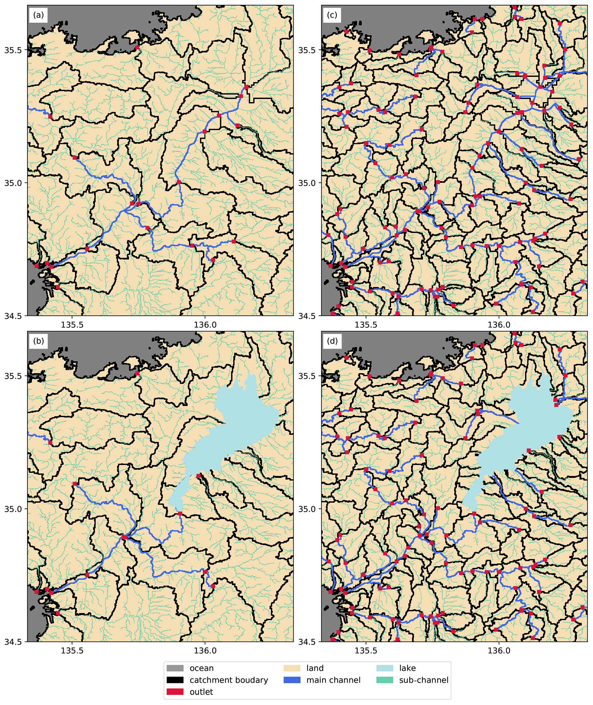
Figure 1 Example of the upscaled river–lake network dataset. The panels show results under four different configurations for Lake Biwa and Yodo River basin in Japan: (a) 15 arcmin without lakes, (b) 15 arcmin with lakes, (c) 6 arcmin without lakes, and (d) 6 arcmin with lakes.

3 Model description

The river–lake network dataset provides fundamental information for use in a framework that couples river and lake models. The network explicitly relates the models to corresponding grids and represents the horizontal connectivity between them. Because the physical schemes used in this study to represent hydro- and thermodynamics in rivers are identical to an existing model (Tokuda et al., 2019), this section focuses on the lake model and the coupling framework after briefly summarizing those riverine schemes.

3.1 River model

The river model used in this study is HEAT-LINK (Tokuda et al., 2019), which is fully coupled with a river routing model, CaMa-Flood (Yamazaki et al., 2011, 2013). This model solves the conservation laws of mass, momentum, and energy for one-dimensional channels.

CaMa-Flood solves the conservation of momentum law by approximating it using a local inertial flow equation, and this enables efficient computation (Bates et al., 2010). The equation is discretized explicitly using a forward-time central-space scheme to simulate the time evolution of the state variables. CaMa-Flood calculates discharges in river channels and floodplains as prognostic variables and diagnoses the cross-sectional shape (e.g., the water depth and area in river channels and adjacent floodplains). This river routing model accounts for fluvial dynamics in river channels and the floodplain with objective parameterization based on high-resolution topographic data. The introduction of floodplain inundation in addition to channel storage tends to reduce changes in water level and leads to improved reproducibility of seasonal discharge variability in large continental rivers, such as the Amazon (Yamazaki et al., 2011).

HEAT-LINK solves water and ice mass and energy conservation laws by calculating heat fluxes, including short- and longwave radiation, sensible heat, latent heat, and frictional heat (Tokuda et al., 2019). The methods used to calculate fluxes are identical to those used in existing studies (Kondo, 1992; Hondzo and Stefan, 1994; Webb and Zhang, 1997). As HEAT-LINK considers varying water surface area and decaying absorption of downward shortwave radiation to water depth, it can represent the role of flood inundation in water temperature changes. By considering the effects of riverine hydrodynamics on thermodynamics, the model properly produces the variability in water temperature not only in ice-free and ice-covered channels but also in regions with bimodal seasonality of water temperature (Tokuda et al., 2019).

3.2 Lake model

A simple one-dimensional lake model was implemented to represent the water budget and thermodynamics in lakes. To reproduce the exchanges between rivers and lakes, the lake model conserves mass and energy while considering horizontal advection in addition to the vertical exchange. All input data, except the meteorological forcing data, were provided by HydroLAKES and the Global Reservoir and Dam Database (GRanD) (Lehner et al., 2011), as described in the following sections.

3.2.1 Hydrodynamics

The lake model used in this study represents seasonal variation in water depth and discharge above a lake bottom elevation derived from HydroLAKES, as the water surface elevation is a downstream boundary condition, and the outflow is an upstream boundary condition for the river model. The water balance in each lake is expressed by the following equation:

$$\begin{array}{}\text{(1)}& {\displaystyle }{\displaystyle \frac{\mathrm{d}S}{\mathrm{d}t}}=P-E+Q_{\text{in}}-Q_{\text{out}}=A(p-e)+Q_{\text{in}}-Q_{\text{out}},\end{array}$$

where S (m³) is the water storage in each lake; t (s) is the time, P and E (m³ s⁻¹) are precipitation and evaporation, respectively; Q_in and Q_out (m³ s⁻¹) are the inflow to and outflow out of the lake, respectively; A (m²) is the lake surface area; and p and e (m s⁻¹) are the precipitation and evaporative loss per area, respectively. Q_in and Q_out also consider backflow at both the lake inlet and outlet. While the precipitation per area is given as input data and the river discharge at the inlet from rivers is calculated by the river model, the outflow and evaporation are calculated from a weir formula and the thermodynamics model in the following section.

This study set geomorphological boundary conditions by estimating the depth–area relationship according to the Global Reservoir Geometry Database (ReGeom) (Yigzaw et al., 2018). In the abovementioned study, the water surface of each reservoir was extracted from satellite images, and the depth–area relationship was estimated to match the total storage of the reservoir registered in GRanD. However, the dataset assumed several shapes for horizontal and vertical cross sections, and the estimation of the surface area and volume of water may have led to large inconsistencies with the reported values for some reservoirs. Therefore, in this study, the vertical shape assumed in the ReGeom was generalized to derive a new depth–area relationship that is consistent with the surface area and volume of water derived from other datasets. In this respect, the area attenuation rate f(r) was calculated by Eq. (2) when $r=z/D_{\mathrm{0}}$, where z is the vertical distance from the origin at the elevation wherein the water surface area is at its maximum, and D₀ is the total depth from the origin to the bottom of the reservoir:

$$\begin{array}{}\text{(2)}& f\left(r\right)=\left\{\begin{array}{ll}(\mathrm{1}-r^{\mathrm{2}})(\mathrm{1}-r{)}^a& (V_{\mathrm{0}}<\mathrm{2}/\mathrm{3}{A}_{\mathrm{0}}{D}_{\mathrm{0}})\\ \mathrm{1}-r^a& (\mathrm{2}/\mathrm{3}{A}_{\mathrm{0}}{D}_{\mathrm{0}}\le V_{\mathrm{0}}<A_{\mathrm{0}}{D}_{\mathrm{0}})\\ \mathrm{1}& (A_{\mathrm{0}}{D}_{\mathrm{0}}\le V_{\mathrm{0}}),\end{array}\right.\end{array}$$

where A₀ (m²) and V₀ (m³) are the surface area and volume of water, respectively, when the water depth is D₀; a is the shape scaling parameter; and D₀, A₀, and V₀ are input from GRanD. a is derived as follows: When $V_{\mathrm{0}}<\mathrm{2}/\mathrm{3}(A_{\mathrm{0}}{D}_{\mathrm{0}}$),

$$\begin{array}{}\text{(3)}& \begin{array}{rl}p& ={\displaystyle \frac{V_{\mathrm{0}}}{A_{\mathrm{0}}{D}_{\mathrm{0}}}}={\displaystyle \frac{a+\mathrm{4}}{(a+\mathrm{2})(a+\mathrm{3})}}\\ & .\dot{}.a={\displaystyle \frac{-\mathrm{5}p+\mathrm{1}+\sqrt{p^{\mathrm{2}}+\mathrm{6}p+\mathrm{1}}}{\mathrm{2}p}};\end{array}\end{array}$$

when $\mathrm{2}/\mathrm{3}\left(A_{\mathrm{0}}{D}_{\mathrm{0}}\right)\le V_{\mathrm{0}}<A_{\mathrm{0}}{D}_{\mathrm{0}}$,

$$\begin{array}{}\text{(4)}& \begin{array}{rl}p& ={\displaystyle \frac{V_{\mathrm{0}}}{A_{\mathrm{0}}{D}_{\mathrm{0}}}}=\mathrm{1}-{\displaystyle \frac{\mathrm{1}}{a+\mathrm{1}}}\\ & .\dot{}.a={\displaystyle \frac{\mathrm{1}}{\mathrm{1}-p}}-\mathrm{1}.\end{array}\end{array}$$

Otherwise (i.e., A₀D₀≤V₀), D₀ was updated as $V_{\mathrm{0}}/A_{\mathrm{0}}$, and a constant depth–area relationship was assumed. The area was also assumed to be constant with respect to water depth for lakes not registered in GRanD.

As the spatial shape of the lakes was obtained from HydroLAKES, the depth–area relationship was also estimated only for those lakes that exhibited consistent volumes in HydroLAKES (attribute name is “Vol_total”) and GRanD (attribute name is “Cap_mcm”). For example, this condition excluded Lake Baikal (HydroLAKES ID 11) where the volumes registered in the two databases were 23 615 000 ×10⁶ m³ and 46 000 ×10⁶ m³, respectively.

This study assumes that the outlet of each lake is a rectangular cross section and applies the weir formula to estimate the outflow Q_out as follows:

$$\begin{array}{}\text{(5)}& {\displaystyle }{\displaystyle }{Q}_{\text{out}}=\mathrm{2}/\mathrm{3}\sqrt{\mathrm{2}g}{C}_{d}B{h}^{\mathrm{3}/\mathrm{2}},\end{array}$$

where g (m s⁻²) is the gravitational acceleration, C_d is a correction coefficient, B (m) is the width of the outlet, and h (m) is the height from the top of the weir to the water surface. A similar formula is used in the existing global model, WaterGAP Global Hydrology Model (WGHM) (Döll et al., 2003; Meigh et al., 1999), but it considers the relationship using a parameter known as “active storage.” Equation (2) assumes a situation in which subcritical flow requires a specific water depth at the overflow section; it then transitions to supercritical flow and forms a free-falling water cascade. In this study, based on the above considerations, the amount of outflow from each lake was calculated in the following three ways:

$$\begin{array}{}\text{(6)}& {\displaystyle }{\displaystyle }{Q}_{\text{out}}=\left\{\begin{array}{ll}kB{h}_{\mathrm{0}}^{\mathrm{3}/\mathrm{2}}& (h_{\mathrm{1}}\le \mathrm{2}/\mathrm{3}{h}_{\mathrm{0}})\\ kB(h_{\mathrm{0}}-h_{\mathrm{1}}{)}^{\mathrm{3}/\mathrm{2}}& (\mathrm{2}/\mathrm{3}{h}_{\mathrm{0}}<h_{\mathrm{1}}\le h_{\mathrm{0}})\\ -kB(h_{\mathrm{1}}-h_{\mathrm{0}}{)}^{\mathrm{3}/\mathrm{2}}& (h_{\mathrm{0}}<h_{\mathrm{1}}),\end{array}\right.\end{array}$$

where k is a correction coefficient (to be set at 5.0 because C_d≈1.7), and h₀ and h₁ (m) are the height of the lake surface and downstream surface from the weir height, respectively. When a lake flows into a river channel, this study assumes that the river water depth in each unit catchment is uniform and gives h₁ as the downstream water depth; otherwise, h₁ is calculated from the surface elevation of the downstream lake or the ocean. Additionally, environmental flow is represented using a simplified method as follows: the minima among (1) 20 % of inflow to lake and (2) discharge to maintain the water depth of the river grid located immediately downstream greater than 0.5 m is considered to be the environmental flow. The model updates the sum of the inflow from all of the inlets for each lake at every (Courant–Friedrichs–Lewy, CFL) time step and then calculates the former value with the total inflow at the previous step. The value is then taken as the outflow when discharge based on the extended weir formula is smaller.

Q_out is supposed to be zero in an inland lake with no outlet. However, preliminary results showed that several inland lakes (e.g., Small Aral Sea, HydroLAKES ID 130) were identified where the water level did not reach equilibrium and continued to increase even after a spin-up calculation due to two factors: (1) the overestimation of riverine inflow caused by a lack of knowledge about some processes including groundwater infiltration and water withdrawals; (2) the absence of negative feedback due to the unavailability of the water depth–area relationship in drier regions, where P−E is negative. In a basin with such a lake, the water level of the surrounding river increases along with the lake due to backflow, resulting in unrealistic ranges (this backflow continues until the inflow to the lake is balanced by the vertical water balance of the lake). In this study, to stabilize the water level of such inland lakes within a realistic range, we calculated the outflow using the method described above and discharged it out of the system. This treatment is identical to that of the river model that does not represent lake dynamics.

3.2.2 Thermodynamics

The lake thermodynamics model implemented in this study is a vertical one-dimensional model in which the water temperature is calculated for each vertical layer; therefore, the horizontal distribution within the lake is not resolved. This model is also able to represent the phase change between water and ice. The vertical structure (i.e., the maximum number of vertical layers and thickness of each layer) is configurable, and the number of active layers and thickness of the bottom layer vary along with lake depth which is defined in order from the water surface to the lake bottom. In the case of a lake that has an area with varying water level as described in Sect. 3.2.1, the volume of each layer is calculated with consideration given to this relationship.

The heat budget of water is expressed using Eq. (7) (Hostetler and Bartlein, 1990):

$$\begin{array}{}\text{(7)}& {\displaystyle }{\displaystyle \frac{\partial T}{\partial t}}={\displaystyle \frac{\mathrm{1}}{A}}{\displaystyle \frac{\partial }{\partial z}}\left(AK{\displaystyle \frac{\partial T}{\partial z}}\right)+{\displaystyle \frac{\mathrm{1}}{c_{\mathrm{w}}{\mathit{\rho }}_{\mathrm{w}}A}}{\displaystyle \frac{\partial \left(A\mathit{\varphi }\right)}{\partial z}},\end{array}$$

where T (^∘C) is the water temperature, z (m) is the depth, A (m²) is the horizontal area of a lake, K (m² s⁻¹) is eddy diffusivity, c_w ($\mathrm{J}{\mathrm{kg}}^{-\mathrm{1}}{}^{\circ }{\mathrm{C}}^{-\mathrm{1}}$) is the specific heat capacity of water, ρ_w (kg m⁻³) is the density of water, and ϕ (W m⁻²) is the shortwave radiation. To calculate K, this study uses the method of Henderson-Sellers (1985), which considers wind-driven diffusion and buoyant convection, and the exponential attenuation of shortwave radiation is used to calculate ϕ (Dake and Harleman, 1969).

The boundary conditions are the heat flux exchanges at the water surface and lake bottom. The heat fluxes at the water surface include up- and downward, short- and longwave, sensible heat, and latent heat. The methods for calculating these fluxes are identical to those of the river model. Assuming a well-mixed condition, the surface temperature of the water is assumed to be the same as the first (uppermost) layer and is not defined as skin temperature. This calculation is only performed when the surface is not completely covered by ice. For the ice–water mixed case, the boundary condition for the surface flux is the weighted mean of the ice-free and ice-covered areas; the boundary condition beneath the ice is the conductive flux between the water and ice. The heat flux from the lake bottom is assumed to be zero, in accordance with existing models (Goudsmit et al., 2002; Hostetler and Bartlein, 1990; Joehnk and Umlauf, 2001).

Many lakes in mid- and high-latitude regions experience ice formation during the winter, and several lake ice models have been developed in past decades (Gu and Stefan, 1990; Hostetler, 1991; Hostetler et al., 1993; Croley and Assel, 1994; Patterson et al., 1998). The representation of the temporal evolution of ice volume in this study is consistent with such models based on the heat budget of the ice. Additionally, this study uses a simplified version of the ice shape parameterization from the Great Lakes Advanced Hydrologic Prediction System (AHPS), a watershed model developed for the Great Lakes region by the Great Lakes Environmental Research Laboratory (GLERL) (Croley and Assel, 1994).

The boundary conditions for the heat budget of the ice cover are that the ice temperature adjacent to the atmosphere T_si (^∘C) and to water T_bi (^∘C) are equal to the atmospheric temperature T_a (^∘C) and melting point of water T_m (=0 ^∘C), respectively:

$$\begin{array}{}\text{(8)}& {\displaystyle }\left\{\begin{array}{l}{T}_{\text{si}}=min\left(T_{\mathrm{a}},T_{\mathrm{m}}\right)\\ T_{\text{bi}}=T_{\mathrm{m}}.\end{array}\right.\end{array}$$

The heat balance at the ice surface is expressed as follows:

$$\begin{array}{}\text{(9)}& {\displaystyle }{\displaystyle }{\mathit{\varphi }}_{\text{dli}}-{\mathit{\varphi }}_{\text{uli}}\left(T_{\text{si}}\right)-{\mathit{\varphi }}_{\text{Hi}}\left(T_{\text{si}}\right)-{\mathit{\varphi }}_{\text{ci}}=\mathrm{0},\end{array}$$

where ϕ_dli, ϕ_uli, ϕ_Hi, and ϕ_ci (W m⁻²) are the downward longwave, upward longwave, sensible, and conductive heat fluxes at the ice surface, respectively.

The temporal change in the ice volume is expressed as follows:

$$\begin{array}{}\text{(10)}& {\displaystyle }{\displaystyle }-{\mathit{\rho }}_{\mathrm{i}}{\mathit{\gamma }}_{\mathrm{i}}{\displaystyle \frac{\mathrm{d}{S}_{\mathrm{i}}}{\mathrm{d}t}}=A_{\mathrm{i}}\left({\mathit{\varphi }}_{\text{ci}}-{\mathit{\varphi }}_{\text{iw}}+{\mathit{\varphi }}_{\text{dsi}}\right),\end{array}$$

where ρ_i (kg m⁻³) is the ice density, γ_i is the fusion heat (=333 500 J kg⁻¹), S_i (m³) is the ice volume, A_i (m²) is the ice area, and ϕ_iw and ϕ_dsi (W m⁻²) are the conductive heat flux from ice to water and the absorption of shortwave radiation by the ice body, respectively. ϕ_iw is calculated using the same method as that of an existing river temperature model (Beek et al., 2012). Our model also assumes that ice loss due to sublimation is negligible according to the GLERL AHPS model (Croley and Assel, 1994).

While a two-dimensional horizontal model computes the ice fraction in each grid in one lake (Goyette et al., 2000), a one-dimensional model such as the TCHOIR needs to consider the ice fraction at a the sub-lake scale. The GLERL AHPS computes the time evolution of ice thickness and area using heat exchange with the atmosphere, water, snowfall, and evaporation. Our study simplified this representation by adding two assumptions: the ice shape change is only caused by exchanging heat with the atmosphere; the thickness of the ice is only determined by area. Under these assumptions, ice thickness is proportional to the square root of the ice area.

The heat budget of water and ice is solved as follows. First, the heat flux from the ice surface to the ice body is calculated by solving the heat balance at the ice surface. With this and the other two fluxes, an increase or decrease in the mass of the ice is calculated. If the ice melts completely in a time step, the heat flux from the ice to the water is recalculated. If there is no ice in a lake, these processes are skipped. The model then computes the heat flux from the water surface to the water body by solving the heat balance at the water surface. For an upper boundary condition of the energy budget of the water body, the model considers shortwave radiation into the body and heat fluxes from the water surface or ice cover, which are different between ice-free and ice-covered areas. Therefore, the model calculates their weighted mean considering the areas. The heat budget of each layer of the water body is solved using an implicit scheme with a staggered grid. In the layers below the melting point, the amount of ice formation is calculated and added to the surface ice. Water from the melted ice is added to the water surface layer.

Because the river model does not solve vertical distributions of mass and heat fluxes within the channel, both rainfall and the water inflowing to a lake are added to the surface layer. The snowfall and ice inflows are also added to the ice cover. The model assumes that the temperature of precipitation is equal to the air temperature, with the minimum temperature of rainfall and maximum temperature of snowfall set to the melting point of water. The model assumes that outflow and evaporative loss consume the water from the surface to the lower layers. The model reanalyzes the ice shape, the layer structures, and the water temperature profile by mixing the temperature of the existing layers from top to bottom, thereby conserving the mass and energy of the water.

3.3 Implementation of coupling interface

3.3.1 Grid system

TCHOIR reads the dataset of a two-dimensional river–lake network derived by the upscaling method described in Sect. 2.2 and then vectorizes it to a one-dimensional array for better computational efficiency. The river grids are arranged in the following order: channel grids from rivers to rivers, lake inlet grids from rivers to lakes, and river mouth grids to the ocean. Following the flow direction, the lake outlet is connected to a river, another lake, or ocean. As the lake outlets and inlets are matched to the outlets of the unit catchments, the discharge at the lake outlets and inlets are calculated using the lake and river model, respectively. These discharges can be negative, which indicates backflow (e.g., a negative value at a lake outlet means that the net water flow is from downstream into the lake).

3.3.2 Data exchanges and communications between model components

As the river and lake models were developed separately, a wrapper interface was required to share interdependent boundary conditions between the sub-models. The TCHOIR framework was built using a coupler that encapsulates the sub-models and ensures topological consistency in time and geography for their communications. Figure 2 shows the sequence of the temporal integrations and data exchange in the coupler. In this study, corrections to the river and lake outflows limit them, ensuring that the outflow is smaller than the storage discharge, which is conducted for river discharge in the original CaMa-Flood. Data exchange between the models occurred prior to correction, which is necessary for some conditions (e.g., backwater).

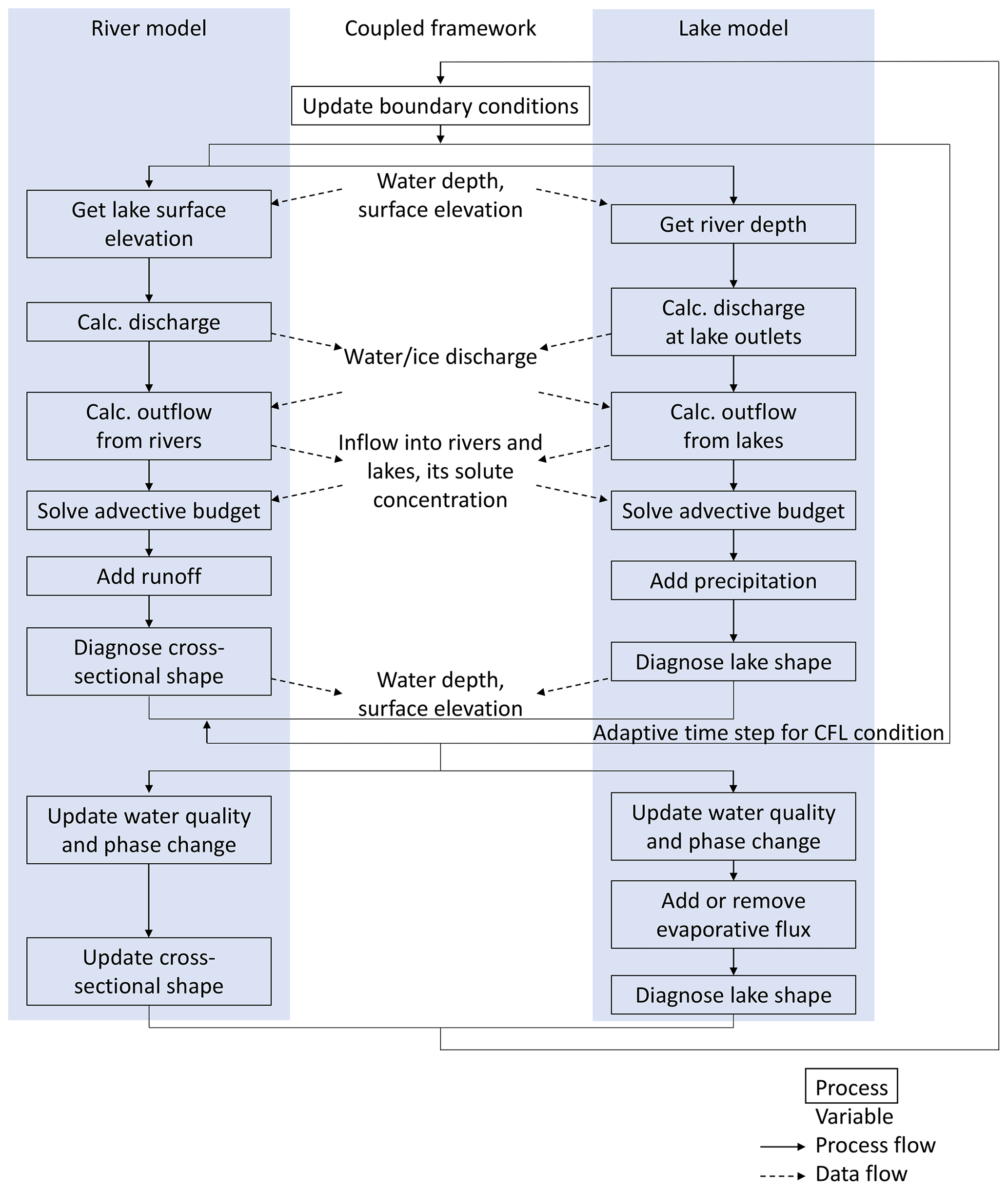
Figure 2 Flowchart of the calculation of TCHOIR. The solid (dashed) arrows indicate the order of the calculations (data exchange). The arrow branches indicate that each process can be computed in parallel, but the data exchange takes place at the same time.

The coupler also shares common information for both models, such as time steps and meteorological forcing data. The time step is determined such that the river model satisfies the CFL condition, and it is used for the lake model as well.

Our framework structure has two significant advantages: (1) encapsulation of stand-alone sub-models, which allows them to be developed or easily replaced, and (2) provision of a convenient test bed to turn each sub-model on or off. In the following section, we compare the results of three experiments to distinguish the interactions between rivers and lakes: “coupled”, “river-only,” and “lake-only.”

4 Validation of harmonized geographical information

This section shows the validation results of the harmonized geographical information by comparing the upstream area with the survey-reported value in GRanD for some reservoirs, instead of the upstream area based on the hydrography information in HydroLAKES. Although the spatial resolution of the following validations of numerical simulations is 15 arcmin, the validation in this section was conducted at a 6 arcmin resolution in order to have a higher number of lakes available for validation (only 14 reservoirs are resolved at a 15 arcmin resolution). The upscaling method implemented in our study conserves the upstream area of the high-resolution input data for all grids; therefore, the upstream areas were identical for lakes resolved between the 6 and 15 arcmin networks.

Figure 3 shows a comparison between the calculated values obtained in this study and the reported values in GRanD for the upstream area of each reservoir. The correlation coefficient was 0.852 for all 103 matched reservoirs. The calculated values of only eight reservoirs were greater than 200 % or less than 50 % of the reported values. Those eight reservoirs are further compared to hydrological data gathered by the United States Geological Survey (USGS) and the Australian National Committee on Large Dams (ANCOLD) (Table 2). In the rest of this section, we discuss three reservoirs that did not agree with the upstream area, both in our data and in other data sources.

Figure 3 Comparison between calculated upstream area (km²) in the river–lake network developed in this study (vertical) and reported values registered in GRanD (horizontal). Red dots indicate the reservoirs whose areas (km²) differ by more than a factor of 2 or 0.5 as listed in Table 2.

Table 2 List of reservoirs whose areas (km²) differ by more than a factor of 2 or 0.5 between calculated and reported upstream values. The ID column provides the lake's identifier in HydroLAKES, and the columns showing the values from the literature and the reference refer to upstream areas described in other literature from GRanD.

Lake Moultrie is located at the uppermost point of the Cooper River basin located in the United States. The Cooper River has a length of 230 km, and the larger Santee River flows through the northern part of the basin. Lake Marion (HydroLAKES ID 828) is located at the confluence of the Wateree River and the Congaree River, which are tributaries of the Santee River. There are two outlets in Lake Marion: one to the Santee River and the other to Lake Moultrie. However, the network developed in this study assumes that each lake only has one outlet according to HydroLAKES, which means that such diversions are not represented. In fact, the reported and calculated values of the upstream area of Lake Marion are almost identical (38 073.0 and 38 060.2 km², respectively), whereas the reported upstream area of Lake Moultrie is more similar to that of Lake Marion. This implies that the reported value of Lake Moultrie includes Lake Marion and its upstream area.

The Cedar Creek Reservoir is located within a subbasin of the Trinity River, and the lake discharge flows into the main stem of the river. However, in the river–lake network dataset developed here, the reservoir is located on the mainstem. This problem is related to flow direction information in MERIT Hydro, and this issue has already been reported to the data developer.

The Iovskoye () reservoir is in the Kovda () river basin. Given the basin map and the fact that the entire Kovda River has a basin area of 25 600 km² (O'Sullivan and Reynolds, 2008), it is considered that the estimate of the upstream area of 19 900.2 km² in this study is reasonable.

5 Validation of integrated simulation framework

5.1 Simulation configuration

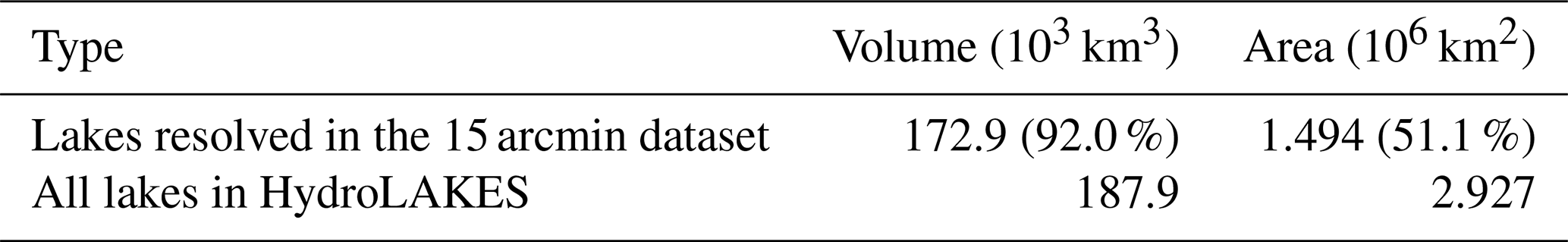
The spatial resolution of the models was set to 15 arcmin, and the river–lake network dataset was upscaled to the same resolution. A total of 369 lakes from around the world were represented at the target resolution, as mentioned in Sect. 2.1. Their area and volume accounted for 51 % and 92 % of the total area and volume of all lakes in HydroLAKES, respectively (Table 3). As described in Sects. 2 and 3, the geomorphic information (e.g., mean depth, mean surface area, and sill height) were obtained from the HydroLAKES and GRanD datasets. The depth–area relationships were defined for 79 out of 369 lakes, and the area of the other lakes was set to be constant.

Table 3 Summary of the lakes resolved in the dataset and all of the lakes in HydroLAKES. (Values in the parentheses indicate the fraction of the resolved lakes to all of the lakes.)

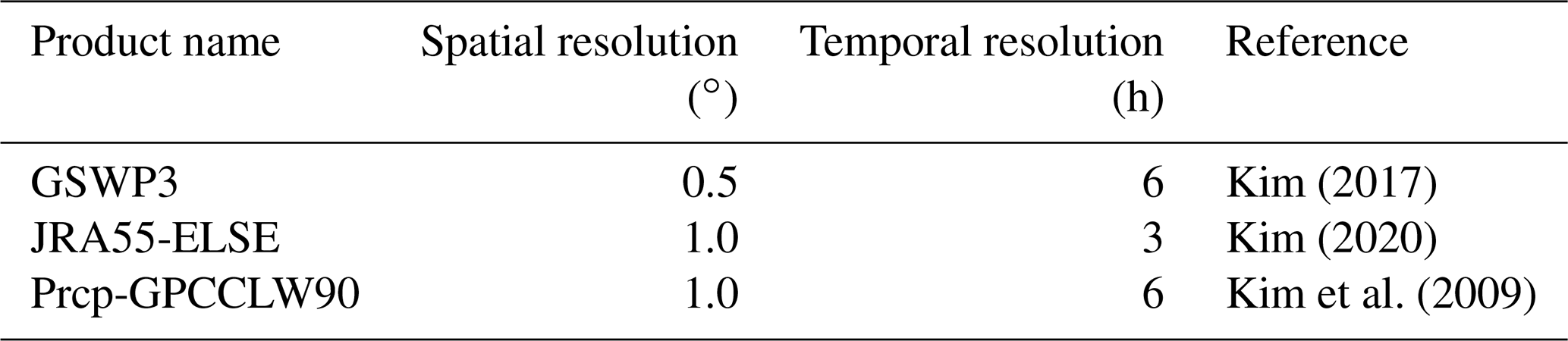
Three different meteorological forcing datasets were prepared to investigate the uncertainty caused by the datasets: GSWP3 (Kim, 2017), JRA55-ELSE (Kim, 2020), and Prcp-GPCCLW90 (Kim et al., 2009). The associated spatiotemporal resolutions are shown in Table 4. To produce the amount and temperature of runoff, a land surface model, MATSIRO (Takata et al., 2003), was employed by using each meteorological forcing dataset. These outputs have the same spatial resolution as the input data (i.e., 0.5, 1, and 1^∘, respectively), and the temporal resolution is 1 d. The main results were based on the GSWP3-forced simulation, and we discuss the sensitivity of the results in Sect. A2.

Table 4 Summary of meteorological forcing data used in this study.

This study assumed constant values for several physical parameters of rivers and lakes. The albedo and attenuation rates for the shortwave radiation of water (ice) were assumed to be 0.1 (0.6) and 0.1 (10.0) m⁻¹, respectively, and the absorption rate of the shortwave radiation at the water surface was set to 0.4. Future research will examine the variation in the parameters by considering other processes including solar zenith angle and water turbidity. Previous studies have proposed empirical equations to calculate outflow for the Great Lakes (Croley and Assel, 1994), which we have adopted. The vertical structure is configured as five layers of 0.2 m, six layers of 0.5 m, eight layers of 2 m, four layers of 5 m, two layers of 10 m, and two layers of 20 m.

The calculation period used in this study was 2000 to 2002, and the spin-up was carried out by repeating the simulation in the year 2000 a total of 20 times. We gave an initial guess of the initial value for lake water level and temperature with the surface elevation in HydroLAKES (attribute name is “Elevation”) and the air temperature (or the water melting point if the air temperature is below it) on the first day of the simulation, respectively, but we manually set initial values for water depth and temperature profile for several lakes to remove the interannual variability in the lake water depth and the bottom temperature after the spin-up. The initial layer thicknesses were calculated by the initial water level and the maximum layer thicknesses given in the configuration file, and the initial ice volume was set to zero.

To observe interactions between rivers and lakes, we conducted two separate experiments, in addition to the coupled experiment. The first used a conventional river model that did not include lakes (the river-only experiment). The river network dataset used in this experiment was slightly different from that used with the coupled experiment due to modification of the outlets of unit catchments to the inlet and outlet of lakes. As this river network was created from the same dataset (MERIT Hydro) using the same algorithm, the comparison should be reasonable. In the second simulation, we turned off the river model and computed only lakes (the lake-only experiment). The simulation ignored the direct flow from one lake into another to exclude the effects of riverine dynamics on lakes.

5.2 Reference data

The framework was validated by comparison with in situ and satellite observation data for the following five variables: (1) river discharge, (2) river temperature, (3) lake surface elevation, (4) lake surface temperature, and (5) vertical profiles of lake temperature. The Pearson correlation coefficient (CORR), bias (BIAS), and root-mean-square error (RMSE) were used in evaluations. Additionally, for river discharge, normalized BIAS and RMSE calculated by the mean observed value (hereafter pBIAS and pRMSE) were used because of the wide range of absolute values.

In situ observation data of river discharge and temperature were collected by the Global Runoff Data Centre (GRDC) and the Global Environmental Monitoring System (GEMS). Validation was performed at a monthly timescale. Stations with datasets longer than a year were selected, which resulted in 148 and 75 of the respective GRDC and GEMS reference sites located downstream of lakes. Stations located upstream were excluded because the backwater effect was negligible (Fig. S1 in the Supplement).

To validate the seasonal change in water surface elevation of the lake, the G-REALM dataset (Birkett et al., 2018) was used. This dataset provides the water surface elevation of lakes with areas greater than 100 km² based on satellite altimetry remote sensing. We used the EGM96 referenced data, which is identical to the MERIT DEM. To identify a lake between the HydroLAKES and G-REALM datasets, latitude and longitude information was used. The consistency of the matched pairs was then manually checked. As a result, 318 out of the 340 lakes in the G-REALM dataset were matched, and 152 lakes were resolved in the river–lake dataset. This validation was performed for 132 lakes that have datasets longer than a year.

For lake surface temperature, the GloboLakes (Carrea and Merchant, 2019) dataset was used. It provides multiple satellite-based estimations at 0.05^∘ global grids on a daily scale for 979 lakes. The observation lake grids were arithmetically averaged to compare with the lake model in this study, which does not represent the horizontal distributions; only quality flags of 4 (acceptable quality) and 5 (best quality) were accepted. This dataset was matched to HydroLAKES using the same method as above, which resulted in 878 matching lakes, 200 of which were resolved in the river–lake network. The validation was performed on 124 lakes that have datasets longer than a year.

The vertical profile of lake water temperature for lakes in North America was validated against The Water Quality Portal (WQP). WQP covers lakes globally, but vertical temperature profiles were only available for the North American region. The comparison between the simulated data and observations is instantaneous because the vertical observations are made only a few times a year. Up to three observation locations were selected for each lake.

5.3 River discharge downstream of lakes

Figure 4 summarizes the reproducibility of river discharge simulated by the TCHOIR framework downstream of the lakes for the coupled and river-only simulations. Overall, it showed an improved performance when the lake was considered (i.e., coupled). However, some rivers showed a limited impact from lakes (e.g., the Lena and Amazon rivers). The impacts were mainly found in two aspects: (1) reduction in the overestimation of discharge and (2) dampening of the amplitude of the seasonal variations in the river-only simulation. For example, at Cornwall station in the St. Lawrence River (Fig. 5a), located downstream of the Great Lakes, discharge from the coupled experiment shows better performance than that of the river-only simulation due to higher evaporative loss at the lake surface, which affects the basin-wide water balance significantly. The reduced seasonality is evident at the Volgograd station of the Volga River, the Manitou Rapids station of the Rainy River, and the Above Kazan Falls station of the Kazan River (Fig. 5b, c, d). In these cases, the incorporation of lakes leads to the dampening of peak discharge because the lake acts as a buffer between flux and storage.

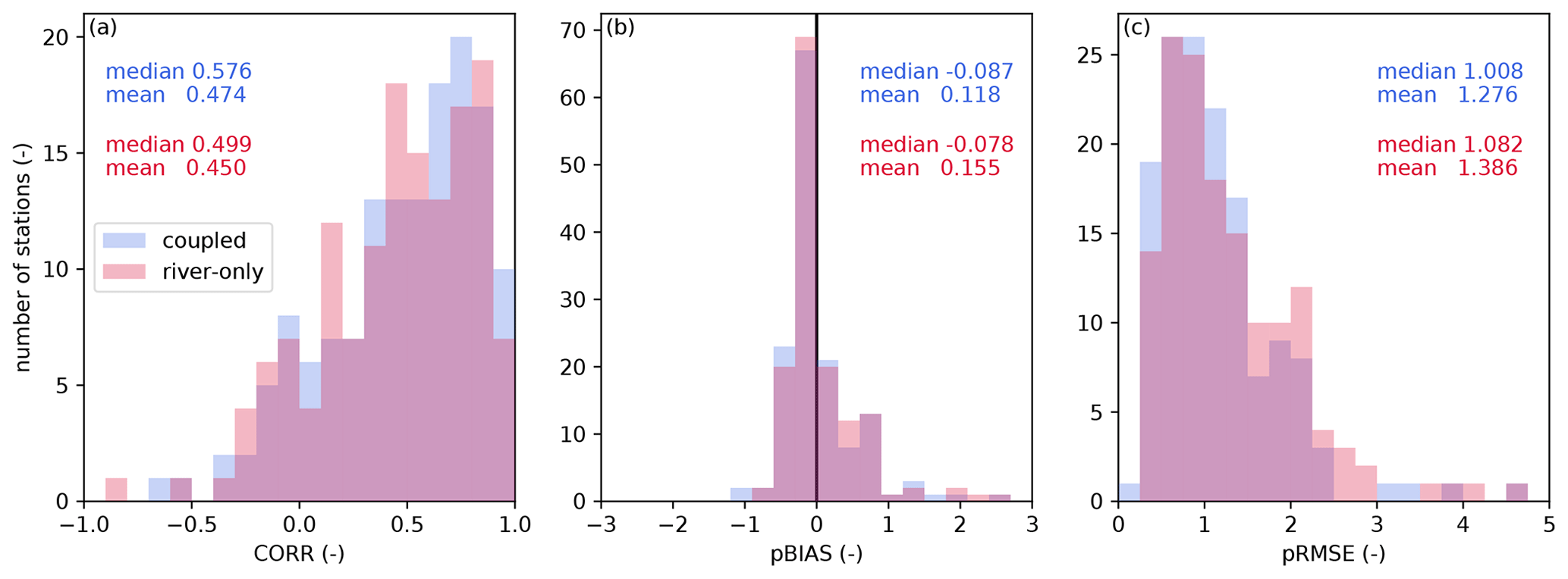
Figure 4 Comparison between reproducibility indices of river discharge. Bars are the histograms of each index, and the numbers indicate the associated median and mean values. Blue (red) bars and written values show the results of the coupled (river-only) simulation. Panel (a) shows CORR, panel (b) shows pBIAS, and panel (c) shows pRMSE.

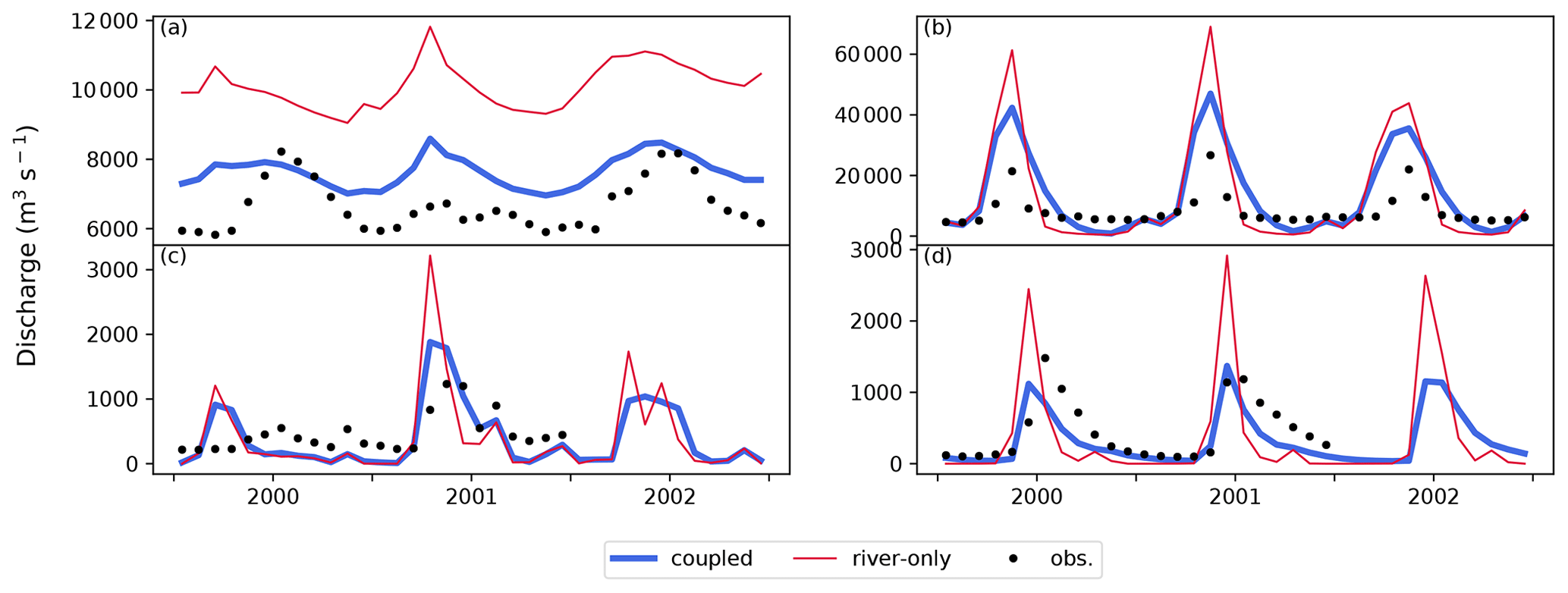
Figure 5 Time series of monthly mean values of river discharge (m³ s⁻¹) for (a) Cornwall station on the St. Lawrence River, (b) Volgograd station on the Volga River, (c) Manitou Rapids station on the Rainy River, and (d) Above Kazan Falls station on the Kazan River. Black dots show the observed values, and blue (red) lines show values calculated by the coupled (river-only) simulation. The GRDC station codes for these stations are 4143550, 6977100, 4213211, and 4214090, respectively.

5.4 River temperature downstream of lakes

The effect of lakes on river temperature is summarized in Fig. 6. It is evident that all performance metrics improved when lakes were presented. Positive or negative river temperature biases were reduced significantly. In particular, for a number of stations in Brazil, coupling of river and lake models reduced the overestimation of water temperature. For example, improvement at 00MS13SM2000 station on the Rio Santa Maria (Fig. 7a) was due to an increase in heat release resulting from an increase in residence time. At Hamilton traffic bridge station on the Waikato River and Puerto Libertad station on the Paraná River, the simulations were improved (Fig. 7b and c, respectively), as warmer water near the surface flows out of lakes due to thermal stratification; moreover, the improvement observed at Puerto Libertad station is significant during the cold season. On the other hand, the incorporation of the lake model led to worse performance for some Russian stations, such as the Neva River and Cheboskarskoye Reservoir stations (station codes RUS00014 and RUS00029, respectively). The former is located downstream of Lake Ladoga (HydroLAKES ID 10), just before it flows into the Gulf of Finland (Fig. 7d). Lake Ladoga is a large lake that spans more than 1.5^∘ north to south. Our framework was unable to capture the temperature peak, especially in summer. We speculate that inflow carrying warmer water from the southern upstream area and the missing representation of sub-lake-scale dynamics may be the cause of such shortcomings and suggest selecting a river scheme for lakes where horizontal flow predominates in addition to vertical mixing. In this respect, a previous study proposed a method for calculating water temperature in lakes using a river model that considers a lake to be a wider river (Beek et al., 2012). A similar shortcoming was found in the Gorkovsky Reservoir (HydroLAKES ID 109).

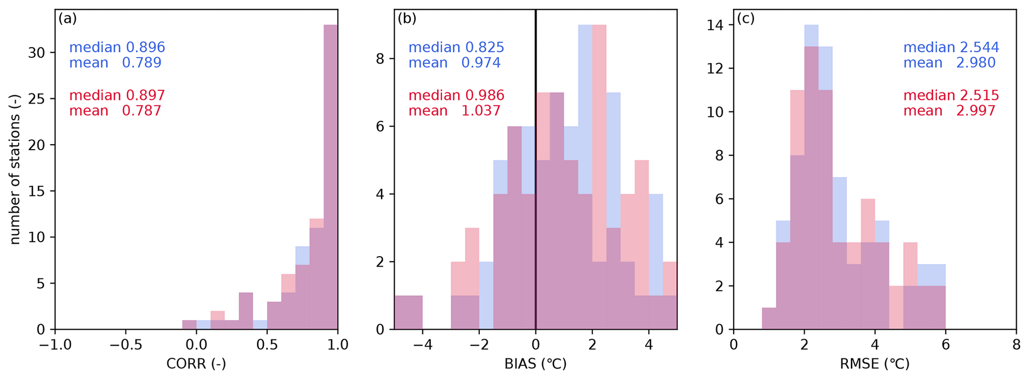
Figure 6 Comparison between reproducibility indices of river temperature. Bars show the histogram of each index, and the numbers indicate associated median and mean values. Blue (red) bars and written values show the result of the coupled (river-only) simulation. Panel (a) shows CORR, panel (b) shows BIAS (^∘C), and panel (c) shows RMSE (^∘C).

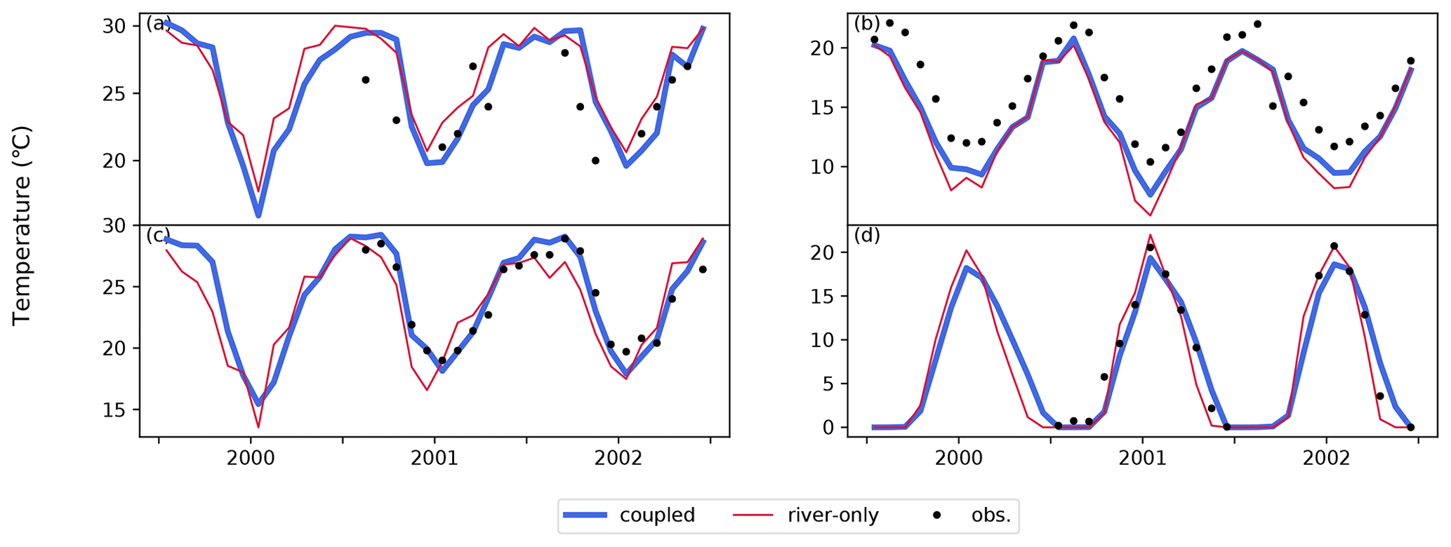
Figure 7 Time series of monthly mean values of river temperature (^∘C). Black dots show the observed values, and blue (red) lines show values calculated by the coupled (river-only) simulation for (a) 00MS13SM2000 station on the Rio Santa Maria, (b) Hamilton traffic bridge station on the Waikato River, (c) Puerto Libertad station on the Paraná River, and (d) Neva River station on the Neva River. The GEMS station codes for these stations are BRA01900, NZL00013, ARG00001, and RUS00014, respectively.

5.5 Lake water surface elevation

The following sections compare the results from the coupled and lake-only experiments. A comparison of the performance metrics (i.e., CORR, BIAS, and RMSE) for the water surface elevation in the 132 lakes is shown in Fig. 8. We noted that the lake-only simulation did not reach an equilibrium state even after the 20-year spin-up, showing a steady increase or decrease (Fig. 9). This is not surprising, given the imbalance between precipitation and evaporation. Therefore, the lake-only simulation is validated only for CORR in Fig. 8. The typical examples are shown in Fig. 9a and b, which present the time series data for Lake Superior and Lake Champlain. The water surface elevations of those lakes keep increasing in the lake-only simulation because of the mass imbalance; precipitation is greater than evaporation, which is consistent with observations (Bennett, 1978; Smeltzer and Quinn, 1996). However, the incorporation of riverine dynamics allows for variation in lake water level within a reasonable range, as the river inflow and outflow play a role in dampening the water level change in lakes. According to Fig. 8a, although the seasonality of the lake surface elevations is dominated by the water budget within the lake (i.e., precipitation minus evaporation), the topographic information surrounding the lakes plays a crucial role in reproducing the absolute value of the water surface elevation in addition to the water budget in between rivers (i.e., in- and outflow). Therefore, applying the coupling framework is potentially beneficial for a long-term Earth system simulation. The coupled simulation also reproduces the range of seasonal variability in Lake Superior. However, the water level in Lake Champlain tends to be overestimated during the wet season. A tuned empirical equation gives the outflow from Lake Superior. At the same time, the model possibly underestimates negative feedback between water level and outflow in Lake Champlain.

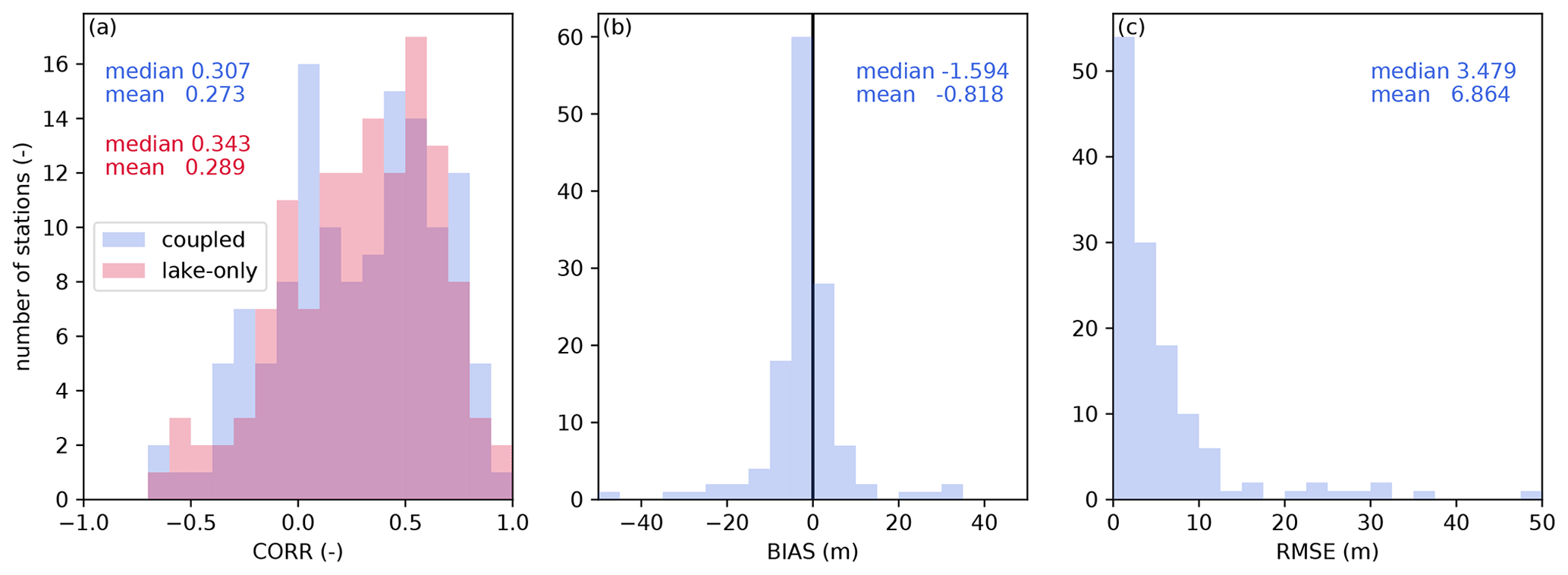
Figure 8 Comparison between reproducibility indices of lake surface elevation. Bars are the histogram of each index, and written values show the associated median and mean values. Blue (red) bars and writing show the results of the coupled (lake-only) simulation. Panel (a) shows CORR, panel (b) shows BIAS (m), and panel (c) shows RMSE (m).

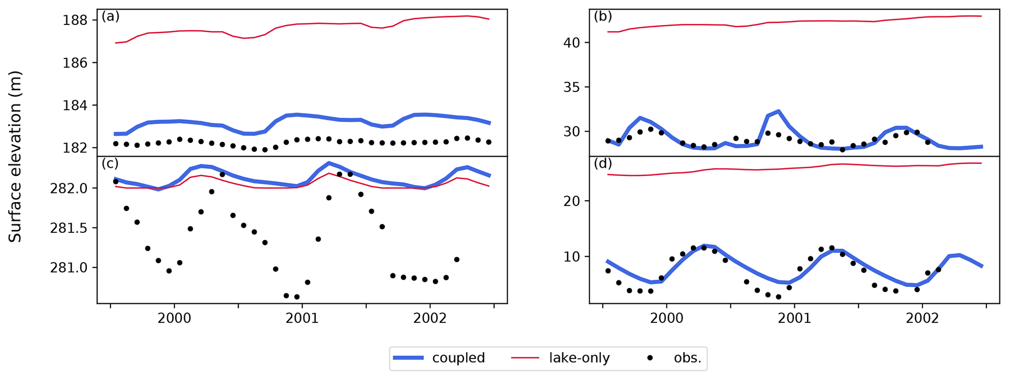
Figure 9 Time series of monthly mean values of lake surface elevation (m) for (a) Lake Superior, (b) Lake Champlain, (c) Lake Chad, and (d) Lake Tonlé Sap (HydroLAKES ID 5, 64, 15, and 153, respectively). Black dots show observed values, and blue (red) lines show values calculated by the coupled (lake-only) simulation.

For Lake Chad (Fig. 9c), both the coupled and lake-only experiments overestimated the water level. The water level was reproduced relatively well during the wet season, but there was a considerable discrepancy between observations. This is because the simulated water level cannot be lower than the given bottom elevation (282 m). To reproduce lake water levels accurately, it is important to treat this lake in two or three parts separately (Gao et al., 2011; Lemoalle et al., 2012). Such topography-induced impacts on lake surface extent and level are rather significant in dry regions. Therefore, a possible solution is to integrate sub-lakes defined based on precise topographic information via the TCHOIR framework.

However, the coupled simulation shows high applicability for use in Lake Tonlé Sap (Fig. 9d). This lake joins the Mekong River in the downstream area, which functions as a natural floodwater reservoir due to backflow from the river during the wet season. Although our framework cannot be compared directly with the water budget of a previous estimation (Kummu et al., 2014) because the river model in this study does not distinguish tributary flows and overland flow, the seasonal change in the simulated outflow from the lake indicates a similar pattern (in which the outflow is negative for several months, mainly from July to September). It is of note that we do not consider temporal changes in the lake area fixed at 2415.98 km², which is within the minimum range of this lake (Kummu et al., 2014).

5.6 Lake surface temperature

Between the coupled and lake-only experiments, the difference in the water temperature estimates was not significant, but the performance measured by the metrics showed slight improvements in the coupled simulation (Fig. 10). The improvement in the bias (BIAS) metric is relatively apparent. Although the lake water storage and heat capacity are significantly larger than the fluvial and thermal inflow (Fig. 11a, b), the riverine impacts on the lake temperature were found during the summer in some lakes (Fig. 11c). In particular, the river flow has a unique impact on lake surface temperature in Lake St. Clair (Fig. 11d); coupling increases the temperature during summer and decreases it during winter. The temperature increase caused by the incorporation of a river model is explained from three perspectives. One is the difference in heat capacity between rivers and lakes, which leads to a larger temperature difference during summer. The second one is a difference in water depth, which affects the shortwave absorption rate per unit volume. Shortwave radiation reaches deeper lake water after attenuation, but shallower river water can effectively absorb radiation. The last mechanism is temperature stratification in upstream lakes, of which the impact is conveyed via rivers. On the other hand, the decrease in temperature Lake St. Clair during winter is caused by cooler riverine inflows from the northern area. We found that the effect also improves the underestimation of a monthly maximum of ice cover fraction in the lake (Sect. A1). Further comparative experiments with a lake model that resolves the spatial distributions of water temperature within a lake would enable us to observe the riverine impact.

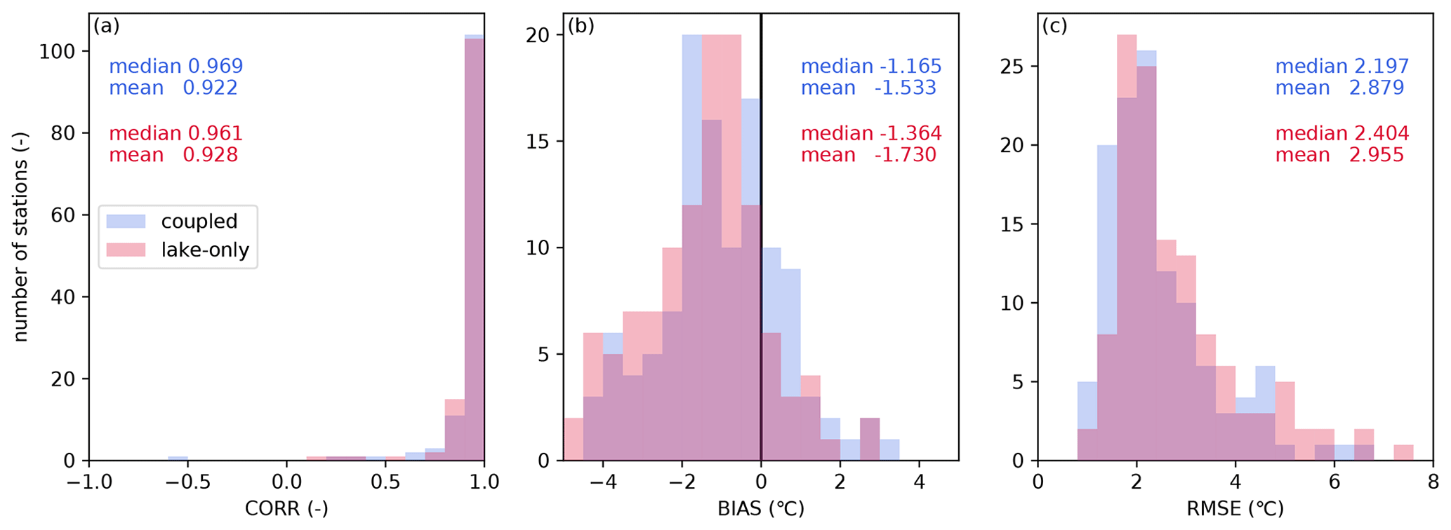
Figure 10 Comparison of reproducibility indices for lake surface temperature. Bars indicate the histogram of each index, and written values show the media and mean values: blue and red indicate the result of the coupled and lake-only simulations, respectively. Panel (a) shows CORR (–), panel (b) shows BIAS (^∘C), and panel (c) shows RMSE (^∘C).

Figure 11 Time series of monthly mean values of river temperature (^∘C) for (a) Lake Superior, (b) Lake Ladoga, (c) Lake Ontario, and (d) Lake St. Clair (HydroLAKES ID 5, 10, 7, and 66, respectively). Black dots show the observed values, and blue (red) lines show the calculated values from the coupled (lake-only) simulation.

5.7 Vertical profile of lake water temperature

Figure 12 shows three representative examples of vertical water temperature profile comparisons. As shown in the results for Lake Ontario and Lake Huron in Fig. 12a and b, respectively, in summer, the vertical water temperature pattern in the upper layers (up to approximately 60 m from the surface) was reproduced well in all lakes. The lake-only simulation also successfully reproduced the profile, and it was found that consideration of riverine in- and outflow alleviated the underestimation of surface temperature, as shown in Sect. 5.6. The observed water depths in all of the Great Lakes (except Lake Erie) are approximately 2-fold the simulated water depth. Previous research focusing on a considerably shallower lake reported that input water depth affects the reproducibility of the lake temperature via heat capacity and vertical diffusion (Stepanenko et al., 2013), whereas our results suggest that the energy exchange at the water surface is the governing factor in the season.

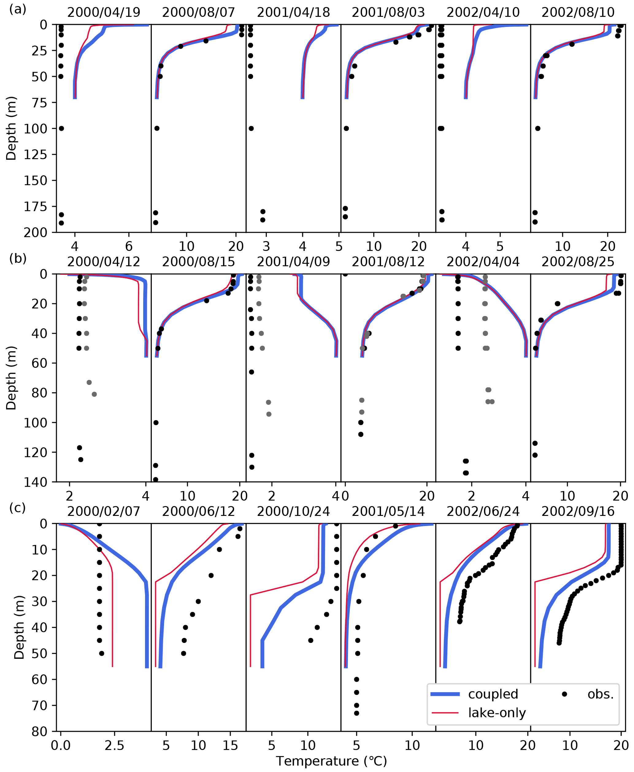
Figure 12 Comparison between vertical water temperature profiles of simulations and observations for (a) Lake Ontario, (b) Lake Huron, and (c) Lake Oahe.

In early spring, however, the model overestimated the temperature. The calculated water temperature near the bottom was close to 4 ^∘C, consistent with the maximum water density assumption at 4 ^∘C, whereas the observed data indicate a slightly lower temperature (2–3 ^∘C). It is known that a greater vertical mixing coefficient leads to a better reproducibility of the lake surface temperature (Gu et al., 2015), but it would not be supposed to improve the overestimation found in Lake Ontario. Therefore, the discrepancy between the observed and simulated temperatures could be attributed to the conductive heat transfer from the bottom sediment requiring further studies to solve the energy budget at the lake bottom.

Even for lakes smaller than the Great Lakes, the models tended to underestimate the temperature near the surface. Figure 12c shows the results for Lake Oahe, where both experiments were shown to have underestimated the temperature near the surface (up to approximately 20 m) in summer, regardless of the difference between calculated and observed water depths. These trends were also observed in the satellite products described in Sect. 5.6.

6 Global distributions of lake impacts on riverine thermodynamics

The impact of reservoir operations and lakes affect downstream flow regimes (Hanasaki et al., 2006; Veldkamp et al., 2017). Figure 13 shows the impacts of lakes on the global distribution of temperature changes in rivers. In most areas, the effect on average temperature is within 1 ^∘C. The inclusion of lakes lowers the river temperatures at high latitudes and in the Nile River basin and raises them in other regions (e.g., Paraná River). It was found that the minimum river water temperature at midlatitudes during the cold season increased with the inclusion of lakes (i.e., coupled). This is because the formation of thermal stratification in lakes warms the water near the surface. The opposite trend is observed in the Nile River, where the increase in heat loss (such as evaporation due to increased residence time) is dominant.

Figure 13 Global distribution of the effect of introducing lakes on river water temperature, calculated by subtracting the simulated value of the river-only experiment that does not consider lakes from the coupled experiment that does (^∘C). Red color indicates that lakes cause an increase in river water temperature. Panel (a) shows the annual mean of the climatological monthly temperature, panel (b) shows the minimum, and panel (c) shows the maximum.

At high latitudes, the minimum water temperature is at the freezing point, and the maximum water temperature decreases (up to 3 ^∘C) in many basins. As Arctic rivers flow across a strong meridional temperature gradient, they play a role in transporting warmer water from upstream areas to colder downstream areas. However, the vertical one-dimensional lake model does not correctly represent such an effect, as the sub-lake-scale dynamics within the lake is not resolved. This impact becomes substantial for larger lakes that span multiple model grids.

7 Discussion for further development

The results discussed so far depend on the implementation of the models used within the integrated framework. While the river model employed in our study is a state-of-the-art model that can be applied on a global scale, it is evident that the lake model requires more improvement compared with previous studies (e.g., representation of the heat budget of bottom sediments and eddy mixing). This section summarizes potential improvements, mainly for the lake model.

The fundamental idea of the coupling framework is to represent only larger lakes in the river–lake network, in order to explicitly represent mass and energy exchanges with rivers upstream and downstream. Our study applied a one-dimensional vertical model to the larger lakes but did not implement a sub-lake-scale model for the other lakes. However, it would be preferable if such a one-dimensional model was applied to smaller lakes from the perspective of the spatial heterogeneity of the actual lakes. Although the river–lake network developed in this study identifies the locations of lake inlets and outlet, the in-lake horizontal hydrodynamics are driven not only by river inflow and outflow but also by the uneven distribution of wind directions caused by surrounding topography and temperature gradients related to spatial heterogeneity of the bottom elevation. Such horizontal mixing could be one reason why there are changes in the optimal parameters or calculation schemes for vertical mixing depending on lake size (Subin et al., 2012). Previous studies have adopted an approach that divides lakes into horizontal grids and applies a vertical one-dimensional model to each column. This does not represent water flow in the horizontal direction. The computational cost of a three-dimensional model (Hodges, 2000) is very expensive when applied globally; hence, the formulation of a simplified physical scheme is suggested. Such a model would contribute to our knowledge of the impacts of rivers on the thermodynamics of lakes, particularly in Arctic regions where incorporating vertical one-dimensional models results in an underestimation of river water temperature. Also, such a model would be well validated by in situ observation data of the vertical temperature profile and a satellite-derived dataset of surface temperature distribution.

This study also assumes that all outflows from lakes come from layers near the water surface. However, to minimize the impact of new dam construction on the ecosystem, some dams are manipulated to release water from a depth with the same temperature as the water entering the reservoir. Furthermore, as highlighted in Sect. 4, while validating the upstream areas of reservoirs, the water balance is affected within and between basins as dam operations are conducted and conduits are built between reservoirs. The latest lake dataset referred to in this study provides detailed information on the spatial distribution of lakes; however, information on outlets from lakes and reservoirs (e.g., location and height) also needs to be extended. Because the outlets of lakes coincide with the most downstream points of each unit-catchment grid in the river–lake network developed in this study, it will be accessible to couple with dam operation models.

We conducted a minimal adjustment to fill the inconsistency between the flow direction of MERIT Hydro and the lake distribution of HydroLAKES, which are developed independently. However, elevation within and near the lakes should be corrected, as MERIT Hydro was corrected according to flow direction and streamlines. In addition to the lake outlet data, such a comprehensive development of the geographical dataset is also essential for the river–lake coupling simulation.

8 Conclusions

Our study was conducted to develop a coupling framework between a river model representing the horizontal flow and a lake model representing a layered structure based on locating lakes on a river network dataset to express the terrestrial hydrological transport of water and energy within the river–lake system. Two high-resolution datasets, MERIT Hydro and HydroLAKES, were merged and upscaled into a hydrological unit-catchment grid system. In our dataset, the upstream area of the reservoir was shown to correlate with the reported values well.

Table 5 Summary of reproducibility indices of coupled simulation. Values in the parentheses are those of the uncoupled (river-only for riverine and lake-only for lacustrine variables) simulation.

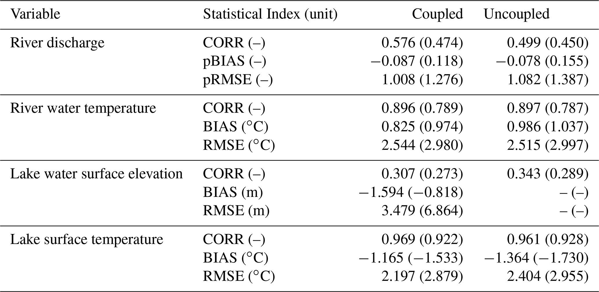
In situ observation data on river discharge and water temperature and satellite datasets on water surface elevation and surface temperature of lakes were used to validate the framework (Table 5). The global results show that the coupled simulation reproduced the absolute values and seasonal variations of those variables better than the individual river model or lake model. The effects of lakes on rivers and vice versa were then discussed by comparing simulation results, which showed better representation in river discharge seasonality when lakes were introduced in the experiment. At sites where lakes occupy a large fraction in their associated basins, such as the Great Lakes region, an increase in evaporative loss from the lakes tended to improve the overestimation of absolute river discharge. It suggests that simultaneous representations of fluvial- and thermodynamics in rivers and lakes are necessary for reliable water availability estimates due to dam construction (Shiklomanov, 2000). The impact of coupling river and lake models on river water temperature has two main aspects: (1) alleviating underestimations in midlatitude regions due to the formation of thermal stratification in lakes, and (2) causing a negative bias at high latitudes because of the missing representation of sub-lake-scale dynamics within a lake suppressing poleward heat transportation by Arctic rivers.

Additionally, the contribution of river inflow and outflow to the water balance of lakes was significant. The seasonal variation in water surface elevation was well reproduced on a global scale. The coupling effects on water surface temperature were not apparent. However, notably, the simulation and validation in this study did not consider spatial variability within lakes, which should be significant in larger lakes. The local energy budget of rivers and lakes is affected by water depth (Stepanenko et al., 2013) and water surface areas (Tokuda et al., 2019). The energy exchanges among them are determined by the combined impacts of their fluvial and thermodynamics. The impact of the water volume changes of lakes and reservoirs has still not been elucidated, even in the latest global study (Vanderkelen et al., 2020), and the modeling framework newly developed in this study, TCHOIR, is expected to estimate a further reliable terrestrial heat budget.

Appendix A

A1 Validation of ice cover in the Great Lakes and Lake St. Clair

We validated the simulated ice cover period and monthly maximum ice fraction in the Great Lakes and Lake St. Clair by comparing them with the dataset provided by GLERL (Assel, 2003; Wang et al., 2012). Except for Lake St. Clair, the coupled and lake-only simulations underestimated the ice cover period in all of the Great Lakes (Fig. A1a), suggesting that the vertical one-dimensional model of lacustrine thermodynamics does not analyze the spatial distribution of the ice cover in larger lakes where the temperature gradient is dominant. It also causes the overestimation of the monthly maximum of the ice cover fraction (Fig. A1b, c, d, e, f). The bias would be improved if parameterization of the ice shape is tuned for those lakes, but implementing a horizontal two-dimensional (three-dimensional give with the vertical one-dimensional) model could be a more straightforward solution. On the other hand, the simulations reproduced the interannual variability of the fraction. In addition, coupling with a river model increased the fraction in Lake Erie and Lake St. Clair, indicating that cooler riverine inflow from the northern area impacts the ice formation in those lakes. Those validations also stress that the efficient three-dimensional lake model is required for global-scale simulation.

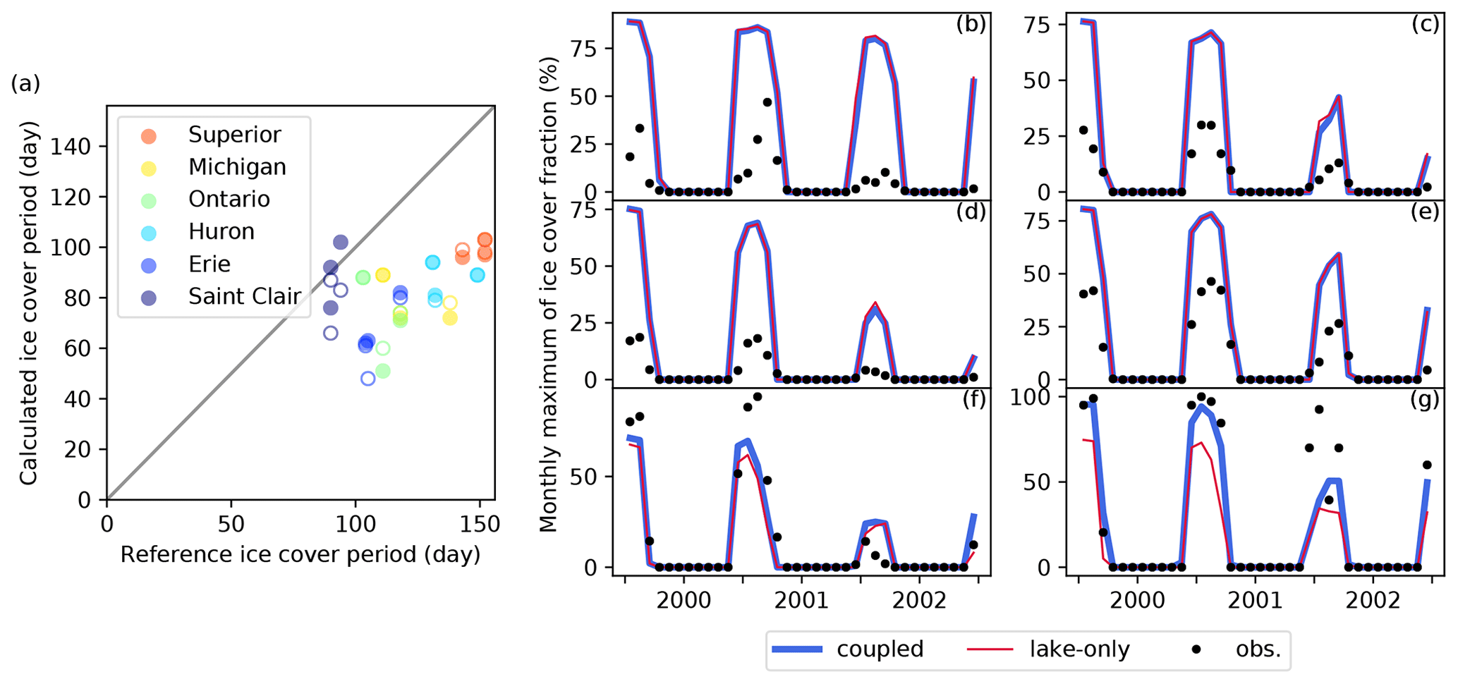
Figure A1 The comparison of (a) the ice cover period in each year (day), and (b–g) the monthly maximum of the ice cover fraction (%) in the Great Lakes region between the simulations and the reference dataset for (b) Lake Superior, (c) Lake Michigan, (d) Lake Ontario, (e) Lake Huron, (f) Lake Erie, and (g) Lake St. Clair (HydroLAKES ID 5, 6, 7, 8, 9, and 66, respectively). (a) The filled (hollow) dots show the results of the coupled (lake-only) simulation. (b–g) Black dots show observed values, and the blue (red) lines show values simulated by the coupled (lake-only) simulation.

A2 Sensitivity to meteorological forcing dataset

We examined the sensitivity of the results to the forcing dataset by comparison with simulations using JRA55-ELSE (Kim, 2020) and Prcp-GPCCLW90 (Kim et al., 2009) forcing datasets in addition to the experiment based on the GSWP3 data. Similar to Sect. 5, Fig. A2 compares the performances of coupled and uncoupled (river-only and lake-only for riverine and lacustrine variables, respectively) simulations forced by those three datasets. All simulations used the same river or river–lake network dataset. The stations subjected to validation are identical to those in Sect. 5.3–5.6.

In general, the results from the sensitivity experiments were similar to those of GSWP3. The CORR and BIAS for river discharge were ameliorated by the inclusion of lakes. The improved reproducibility in river water temperature was found in the coupled mode for all forcing datasets. Stable reproducibility of the lake surface elevation was found to be robust for the forcing datasets. Although incorporating the river model improved the underestimation of the lake surface temperature, a systematic bias is observed for lakes where the model overestimates the temperature. These under- and overestimation patterns can be attributed to the difference in river and lake water heat capacity. Shallow water depth in rivers leads to warmer temperatures due to the more effective absorption of shortwave radiation. A better representation of vertical mixing may reduce such underestimation, leading to further realistic heat exchanges with the atmosphere.

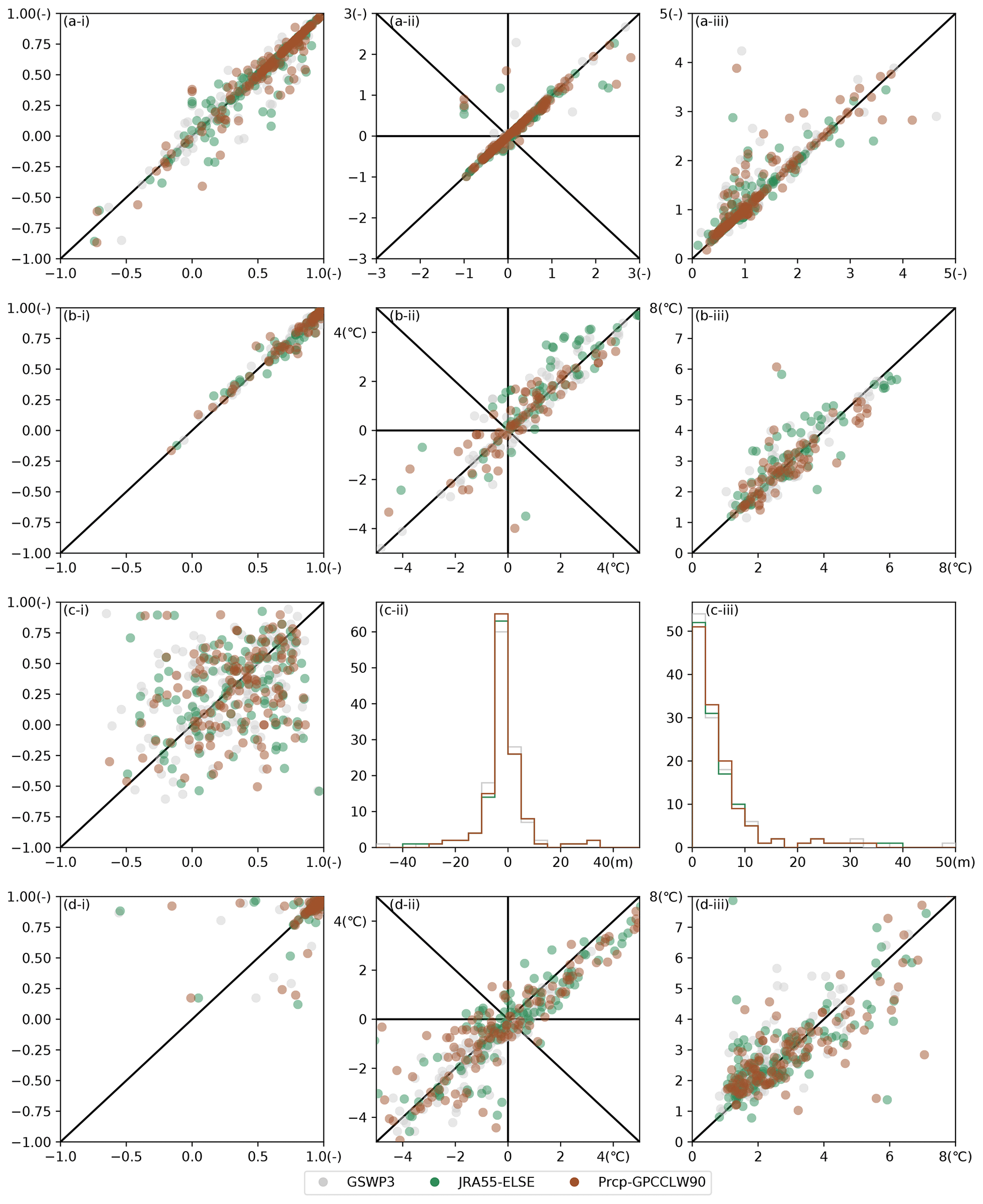
Figure A2 Sensitivity of the performance metrics to the meteorological forcing datasets. The horizontal and vertical axes indicate the results of coupled and uncoupled (river-only for a and b, lake-only for c and d) simulations, respectively. Gray, green, and brown colors indicate the results of GSWP3, JRA55-ELSE, and Prcp-GPCCLW90, respectively, for (a) river discharge, (b) river water temperature, (c) lake surface elevation, and (d) lake surface temperature. The panels labeled (i) show CORR, the panels labeled (ii) show BIAS, and the panels labeled (iii) show RMSE. BIAS and RMSE are normalized for river discharge. BIAS and RMSE of the lake surface elevation in the lake-only simulation are not shown due to the drift even after spin-up.