Implementation of sequential cropping into JULESvn5.2 land-surface model

Land-surface models (LSMs) typically simulate a single crop per year in a field or location. However, actual cropping systems are characterized by a succession of distinct crop cycles that are sometimes interspersed with long periods of bare soil. Sequential cropping (also known as multiple or double cropping) is particularly common in tropical regions, where the crop seasons are largely dictated by the main wet season. In this paper, we implement sequential cropping in a branch of the Joint UK Land Environment Simulator (JULES) and demonstrate its use at sites in France and India. We simulate all the crops grown within a year in a field or location in a seamless way to understand how sequential cropping influences the surface fluxes of a land-surface model. We evaluate JULES with sequential cropping in Avignon, France, providing over 15 years of continuous flux observations (a point simulation). We apply JULES with sequential cropping to simulate the rice–wheat rotation in a regional 25 km resolution gridded simulation for the northern Indian states of Uttar Pradesh and Bihar and four single-grid-box simulations across these states, where each simulation is a 25 km grid box. The inclusion of a secondary crop in JULES using the sequential cropping method presented does not change the crop growth or development of the primary crop. During the secondary crop growing period, the carbon and energy fluxes for Avignon and India are modified; they are largely unchanged for the primary crop growing period. For India, the inclusion of a secondary crop using this sequential cropping method affects the available soil moisture in the top 1.0 m throughout the year, with larger fluctuations in sequential crops compared with single-crop simulations even outside the secondary crop growing period. JULES simulates sequential cropping in Avignon, the four India locations and the regional run, representing both crops within one growing season in each of the crop rotations presented. This development is a step forward in the ability of JULES to simulate crops in tropical regions where this cropping system is already prevalent. It also provides the opportunity to assess the potential for other regions to implement sequential cropping as an adaptation to climate change.

1 Introduction

Climate change is likely to impact all aspects of crop production, affecting plant growth, development and crop yield (Hatfield and Prueger, 2015) as well as cropping area and cropping intensity (Iizumi and Ramankutty, 2015). The impact of climate change on agriculture has been the focus of several large collaborative projects such as the Agricultural Model Intercomparison and Improvement Project (AgMIP; Rivington and Koo, 2010; Rosenzweig et al., 2013, 2014) and the Inter-Sectoral Impact Model Intercomparison Project (ISIMIP; Warszawski et al., 2013, 2014). These projects have highlighted the likelihood of competition between crops grown for food and those grown for bio-energy in order to mitigate climate change (Frieler et al., 2015). Petrie et al. (2017) discuss how the use of sequential cropping systems may have made it possible for populations in some areas to adapt to large changes in monsoon rainfall between 2200 and 2100 BC. These ancient agricultural practices are common today across most tropical countries but may also be a useful adaptation in areas where traditionally mono-crop systems are used, in order to meet a future rising demand for food (Hudson, 2009) or the demand for bio-fuels. This sort of adaptation is already happening in some locations. Mueller et al. (2015) show that longer growing seasons in the extratropics have made the cultivation of multiple crops in a year at northern latitudes more viable. Warmer spring temperatures in the Brahmaputra catchment have allowed earlier planting of a winter crop, leaving time for a second crop (Zhang et al., 2013).

The economy of South Asia is highly dependent on the agricultural industry and other industries also with a high demand for water (Mathison et al., 2015). The most important source of water for this part of the world is the Asian summer monsoon (ASM), which typically occurs between June and September (Goswami and Xavier, 2005); this phenomenon provides most of the water resource for any given year. The South Asian crop calendar is defined by the ASM, which has an important influence on the productivity across the whole year (Mathison et al., 2018), thereby affecting crop production outside the monsoon period.

Intercropping or sequential cropping allow farmers to make the most efficient use of limited resources and space in order to maximize yield potential and lower the risk of complete crop failure. These techniques also influence ground cover, soil erosion and chemical properties, albedo and pest infestation (Waha et al., 2013). Intercropping is the simultaneous cultivation of multiple crop species in a single field (Cong et al., 2015), while sequential cropping (also called multiple or double cropping) involves growing two or more crops on the same field in a given year (Liu et al., 2013; Waha et al., 2013). We use the term sequential cropping from here on to avoid confusion with other cropping systems. Sequential cropping systems are common in Brazil where the soybean–maize or soybean–cotton rotations are used (Pires et al., 2016) and for South Asia where the rice–wheat systems are the most extensive, dominating in many Indian states (Mahajan and Gupta, 2009), across the Indo-Gangetic Plain (IGP) (Erenstein and Laxmi, 2008) and Pakistan (Erenstein et al., 2008). States such as Punjab, Haryana, Bihar, Uttar Pradesh and Madhya Pradesh (Mahajan and Gupta, 2009) account for approximately 75 % of national food grain production for India. Rice–rice rotations are the second most prevalent crop rotation to rice–wheat rotations; these are typically found in the northeastern regions of India and Bangladesh (Sharma and Sharma, 2015), with some regions cultivating as many as three rice crops per year.

1.1 Modelling sequential cropping in land-surface models

The modelling of crop rotations is a regular feature of soil carbon simulations (Bhattacharyya et al., 2007). Bhattacharyya et al. (2007) found that the rice–wheat rotation, common across the IGP, has helped maintain carbon stocks. However, in recent years, the yields of rice and wheat have plateaued, leading farmers to diversify and include other additional crops in the rotation, potentially depleting carbon stocks. The modelling of crop rotations has also been represented in the field of agricultural economics with work regarding sequential cropping being mainly to understand influences on decision-making, therefore focusing on short timescales and at the farm management level (Dury et al., 2012; Caldwell and Hansen, 1993).

Many dynamic global vegetation models (DGVMs), used to study the effects of climate change, simulate a single crop in a field per year, both for individual sites and gridded simulations. This may be due in part to some global observation datasets such as Sacks et al. (2010) reporting only one growing period per year at a given location for most crops (Waha et al., 2012). Where different crop calendars are available for different regions, e.g. MIRCA2000 (Portmann et al., 2010), rice and wheat are divided equally between the kharif (i.e. sown during the monsoon and harvested during the autumn) and rabi seasons (i.e. the drier winter/spring growing season), when in reality wheat is only grown during the rabi season (Biemans et al., 2016).

The Lund–Potsdam–Jena managed land model (LPJml; Bondeau et al., 2007; Schaphoff et al., 2018) is one of the few models that is able to simulate sequential cropping. Waha et al. (2013) extend LPJml to consider sequential cropping in Africa for two different crops on the same field within a year. Waha et al. (2013) specify different growing periods for each crop in the rotation, where the growing period is calculated from the sum of the daily temperatures above a crop-specific temperature threshold. Waha et al. (2013) use the Waha et al. (2012) method to specify the onset of the main rainy season as the start of the growing season, where growing season is defined as the period of time in which temperature and moisture conditions are suitable for crop growth. The growing period of the first crop in the rotation begins on the first wet day of the growing season, with the second crop assumed to start immediately after harvest of the first crop. Waha et al. (2013) find that when considering the impact of climate change, the type of cropping system is important because yields differ between crops and cropping systems. Biemans et al. (2016) also use a version of LPJml refined for South Asia to estimate water demand and crop production for South Asia. Biemans et al. (2016) combine the output from two separate simulations, each with different kharif and rabi land-use maps and zonal sowing and harvest dates based on observed monsoon patterns. Biemans et al. (2016) find that accounting for multiple different crops being grown on the same area at different times of the year improves the simulations of demand for water for irrigation, particularly the timing of the demand. Waha et al. (2013) and Biemans et al. (2016) simulate more than one crop growing on the same area using very different methods; both have highlighted the importance of representing this type of cropping system.

Garrigues et al. (2015a) demonstrate that the Interactions between the Soil, Biosphere and Atmosphere (ISBA) land-surface model (LSM) (Noilhan and Planton, 1989), specifically ISBA-A-gs (Calvet et al., 1998), is able to represent a 12-year succession of arable Mediterranean crops for a site in Avignon, France (Garrigues et al., 2015a, b). This type of cropping system is not typically represented in LSMs; however, this study showed that the implementation of crop successions in an LSM leads to a more accurate representation of cumulative evapotranspiration over the 12-year period. It would be beneficial for more land-surface models to develop the capability to simulate different cropping systems and link crop production with irrigation both to improve the representation of the land surface in coupled models and to improve climate impacts assessments.

In this paper, we describe and implement sequential cropping in the Joint UK Land Environment Simulator (JULES). We simulate the same Avignon site described in Garrigues et al. (2015a, 2018) and two states in India to illustrate and evaluate the method implemented in the JULES stand-alone model at version 5.2 for simulating sequential-crop rotations. By using Avignon and India, we simulate two types of crop rotation. We define the Avignon crop rotation as an irregular crop rotation due to the occurrence of long fallow periods, with extended periods of bare or almost bare soil. There are no long fallow periods in the rice–wheat rotation for the northern Indian states of Uttar Pradesh and Bihar, so we refer to this as a regular crop rotation. The rice–wheat rotation is the dominant cropping system for Uttar Pradesh and Bihar, with these states being key producers of these crops. Sequential cropping is used in a series of single-grid-box simulations (where each grid box is 25 km) across these two states for comparison with a point simulation in Avignon. We also use sequential cropping in a regional 25 km resolution gridded simulation to demonstrate that this method can be applied at larger scales. In the India simulations (both the regional and single grid box), the model uses standard soil parameters, with meteorological information provided from a regional climate simulation (Sect. 3.2). However, for the point simulation in Avignon, we use the site characteristics and meteorological information from the site itself (Sect. 3.1). This paper is structured as follows: Sect. 2 describes the JULES-crop model, the rationale and the method for implementing sequential cropping in JULES. The simulations are described in Sect. 3. In Sect. 4, we present our hypotheses for assessing the impact of sequential cropping in JULES, discuss the climate of the simulated regions and describe the observations we use to evaluate the model. The results from the evaluation of the simulations and the assessment of the impact of sequential cropping are provided in Sect. 5 and discussed in Sect. 6, with conclusions in Sect. 7.

Table 1 JULES flags used that are new or different from those in Osborne et al. (2015).

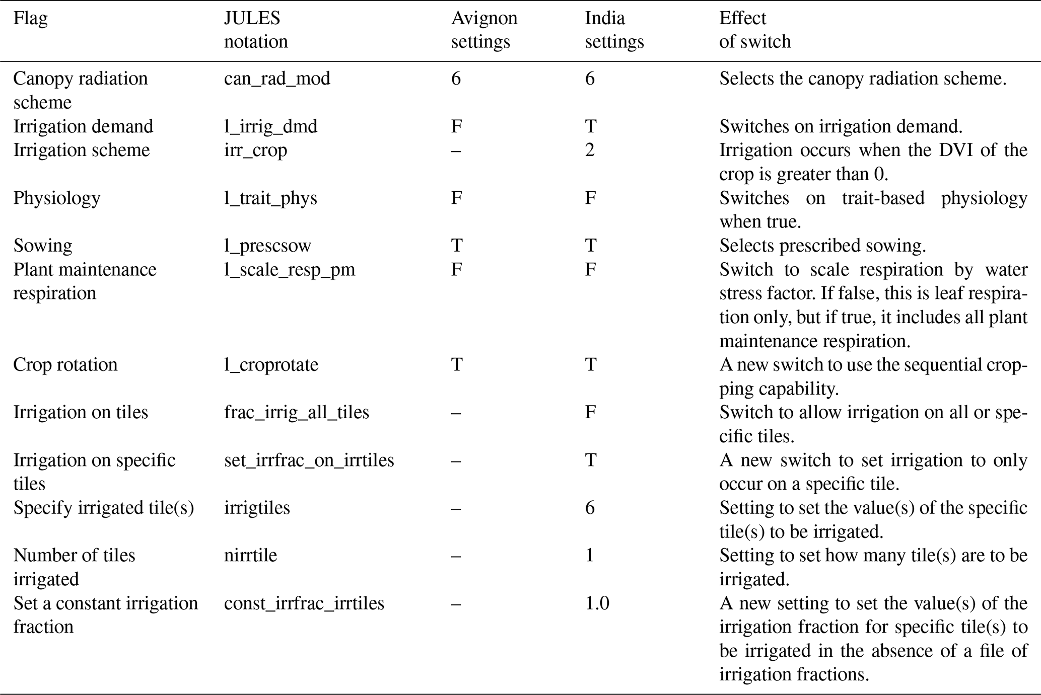
Table 2 JULES plant functional type (PFT) parameters and values modified for use in this study. We include only the values that have been changed or are new in JULES since Osborne et al. (2015).

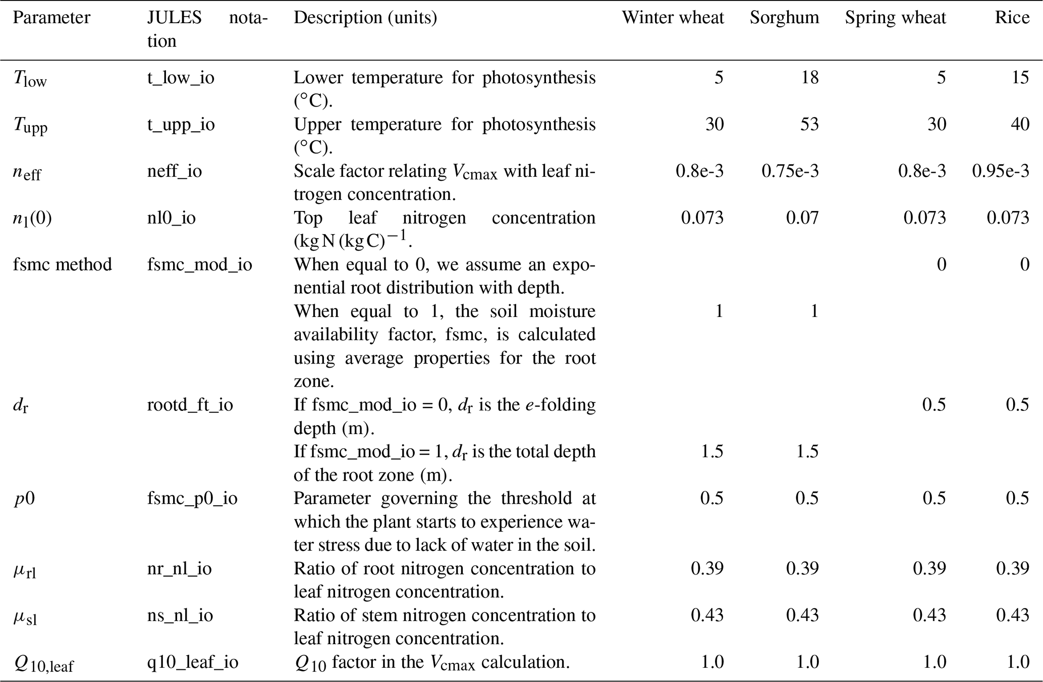
Table 3 JULES crop parameters used in this study. The sorghum cardinal temperatures are from Nicklin (2012) with the other parameters being those used for maize in Osborne et al. (2015). We include only the values that have been changed or added since Osborne et al. (2015). Table 3 of Osborne et al. (2015) provides the original PFT parameters and Table 4 of Osborne et al. (2015) provides the original crop parameters.

2 The JULES-crop model

2.1 Model description

The JULES model is the land-surface scheme used by the UK Met Office for both weather and climate applications. It is also a community model and can be used in stand-alone mode, which is how it is used in the work presented here. The parameterization of crops in JULES (JULES-crop) is described in Osborne et al. (2015) and Williams et al. (2017). JULES-crop is a dual-purpose crop model intended for use within stand-alone JULES, enabling a focus on food production and water availability applications, and as the land-surface scheme within climate and Earth system models. JULES-crop has been used in stand-alone mode in recent studies such as Williams and Falloon (2015) and Williams et al. (2017). The aim is that these studies and this one will lead to using JULES in these larger models to allow the feedbacks from regions with extensive croplands and irrigation systems, like South Asia, to have an effect on the atmosphere, e.g. via methane emissions from rice paddies or evaporation from irrigated fields (Betts, 2005).

JULES is a process-based model that simulates the fluxes of carbon, water, energy and momentum between the land surface and the atmosphere. JULES represents both vegetation (including natural vegetation and crops) and non-vegetation surface types including; urban areas, bare soil, lakes and ice. With the exception of the ice tile, all these tiles can co-exist within a grid box so that a fraction of the surface within each grid box is allocated between surface types. For the ice tile, a grid box must be either completely covered in ice or not (Shannon et al., 2019). JULES treats each vegetation type as a separate tile within a grid box, with each one represented individually with its own set of parameters and properties, such that each tile has a separate energy balance. The model and the equations it is based on are described in detail in Best et al. (2011) and Clark et al. (2011). Prognostics such as leaf area index (LAI) and canopy height are therefore available for each tile. The forcing air temperature, humidity and wind speed are prescribed for the grid box as a whole for a given height. Below the surface, the soil type is also uniform across each grid box (where the number of soil tiles is set to 1). We use JULES-crop (Osborne et al., 2015; Williams et al., 2017) to simulate the crops in this study. The main aim of JULES-crop is to improve the simulation of land–atmosphere interactions where crops are a major feature of the land surface (Osborne et al., 2015).

Photosynthesis in JULES-crop uses the same parameters and code as the natural plant functional types (PFTs). There are two temperature parameters: T_low and T_upp; these define the upper and lower temperature parameters for leaf biochemistry and photosynthesis within JULES (Clark et al., 2011) and are used to calculate the maximum rate of carboxylation of RuBisCO (unstressed by water availability and ozone effects – V_cmax, with units of $\mathrm{mol}{\mathrm{CO}}_{\mathrm{2}}{\mathrm{m}}^{-\mathrm{2}}{\mathrm{s}}^{-\mathrm{1}}$), as defined in Clark et al. (2011) and reproduced here in Eq. (1). Equation (1) demonstrates the V_cmax at any desired temperature.

$$\begin{array}{}\text{(1)}& {\displaystyle }& {\displaystyle }{V}_{\text{cmax}}={\displaystyle \frac{n_{\text{eff}}{n}_{\mathrm{l}}\left(\mathrm{0}\right)f_T\left(T_{\mathrm{c}}\right)}{\left[\mathrm{1}+{\mathrm{e}}^{\mathrm{0.3}(T_{\mathrm{c}}-T_{\text{upp}})}\right]\left[\mathrm{1}+{\mathrm{e}}^{\mathrm{0.3}(T_{\text{low}}-T_{\mathrm{c}})}\right]}}\text{(2)}& {\displaystyle }& {\displaystyle }{f}_T\left(T_{\mathrm{c}}\right)=Q_{{\mathrm{10}}_{\text{leaf}}}^{\mathrm{0.1}(T_{\mathrm{c}}-\mathrm{25})},\end{array}$$

where f_T is the standard Q₁₀ temperature dependence (given in Eq. 2) and T_c is the canopy temperature. n_eff represents the scale factor in the V_cmax calculation (in units of $\mathrm{mol}{\mathrm{CO}}_{\mathrm{2}}{\mathrm{m}}^{-\mathrm{2}}{\mathrm{s}}^{-\mathrm{1}}\mathrm{kg}\mathrm{C}(\mathrm{kg}\mathrm{N}{)}^{-\mathrm{1}}$) and n_l(0) the top leaf nitrogen concentration (in units of kg N (kg C)⁻¹). More details regarding the calculation of V_cmax are provided in Clark et al. (2011) and Williams et al. (2017). V_cmax is an important component in two limiting factors for photosynthesis: the RuBisCO-limited rate and the rate of transport of photosynthetic products; Eq. (1) shows the relationship between V_cmax and temperature. Gross primary productivity (GPP) is used to describe the total productivity of a plant; this defines the gross carbon assimilation in a given time. Net primary productivity (NPP) is GPP minus plant respiration; NPP is used in the crop partitioning code and subsequently in the calculation of the yield in JULES. The nitrogen cycle in JULES cannot yet be used with the crop model, so in this study the same assumption is made as in Williams et al. (2017): that crops are not nitrogen limited.

The effective temperature (Eq. 3) is the function that the model uses to relate air or leaf temperature to the cardinal temperatures that define a plant's development; these are the base temperature (T_b), maximum temperature (T_m) and optimum temperature (T_o) and are specific for each crop. Different models define their effective temperature function in different ways; for example, Fig. 1 of Wang et al. (2017) provides a number of different possible definitions. The JULES definition described by Eq. (3) is most similar to type 4 given in Wang et al. (2017). Type 4 increases gradually towards the optimum temperature with a steeper decline from the optimum to the maximum. Other functions have no decline or a flatter top, which can have different effects on the development of the crop. In JULES, the cardinal temperatures and the 1.5 m tile (i.e. air) temperature (T) are used to calculate the thermal time, i.e. the accumulated effective temperature (T_eff) to which a crop is exposed (Osborne et al., 2015). Table 3 summarizes the settings for these temperatures used in this analysis. The crop model integrates an effective temperature over time as the crop develops through these stages, with the carbon partitioned according to the development index (DVI).

$$\begin{array}{}\text{(3)}& {\displaystyle }{\displaystyle }{T}_{\text{eff}}=\left\{\begin{array}{lcl}\mathrm{0}& \text{for}& T<T_{\mathrm{b}}\\ T-T_{\mathrm{b}}& \text{for}& T_{\mathrm{b}}\le T\le T_{\mathrm{o}}\\ {\displaystyle }(T_{\mathrm{o}}-T_{\mathrm{b}})(\mathrm{1}-{\displaystyle \frac{T-T_{\mathrm{o}}}{T_{\mathrm{m}}-T_{\mathrm{o}}}})& \text{for}& T_{\mathrm{o}}<T<T_{\mathrm{m}}\\ \mathrm{0}& \text{for}& T\ge T_{\mathrm{m}}\end{array}\right.\end{array}$$

The DVI is a function of the thermal time since emergence; therefore, DVI of −1 is sowing, 0 is emergence, and 1 is flowering. Maturity and therefore harvest occur at a DVI of 2 (Osborne et al., 2015) under standard growth conditions but may be harvested earlier in other situations in the model (Williams et al., 2017). In reality, the maturity date and the harvest dates are not usually the same date. The integrated effective temperature in each development stage is referred to as the thermal time of that development stage (Eq. 3 and Osborne et al., 2015; Mathison et al., 2018).

Crop development can also be affected by the length of the day. However, in these simulations, as in Osborne et al. (2015), this effect is not included. The thermal time is then used to calculate the rate of crop development or rate of increase of the development index, described by Eq. (4):

$$\begin{array}{}\text{(4)}& {\displaystyle }{\displaystyle \frac{\mathrm{d}\text{DVI}}{\mathrm{d}t}}=\left\{\begin{array}{lcl}\frac{T_{\text{eff}}}{{\mathrm{TT}}_{\text{emr}}}& \text{for}& -\mathrm{1}\le \text{DVI}<\mathrm{0}\\ \left(\frac{T_{\text{eff}}}{{\mathrm{TT}}_{\text{veg}}}\right)& \text{for}& \mathrm{0}\le \text{DVI}<\mathrm{1}\\ \frac{T_{\text{eff}}}{{\mathrm{TT}}_{\text{rep}}}& \text{for}& \mathrm{1}\le \text{DVI}<\mathrm{2},\end{array}\right.\end{array}$$

where TT_emr is the thermal time between sowing and emergence, TT_veg and TT_rep are the thermal time between emergence and flowering and between flowering and maturity, respectively. These are calculated either using a temperature climatology from the driving data and sowing dates from observations or using the method presented in Mathison et al. (2018) to create a reliable sowing and harvest dataset. The advantage of using the Mathison et al. (2018) method is that there are no missing data, which is often the case when using observed data. Whichever source of sowing and harvest dates are used, the aim is for the crop to reach maturity, on average by the harvest date. The sowing and harvest dates used in the simulations in this analysis are described in Sect. 3.

2.2 Implementing sequential cropping in JULES-crop

2.2.1 JULES-crop: rationale for implementing sequential cropping in JULES-crop

JULES-crop is typically run as a single-crop model, represented by the red curve in Fig. 1, where a primary crop is simulated but no second crop is possible, and the land is left fallow with a minimum surface cover. In many regions, sequential cropping is the main cropping system used, with several crops cultivated one after another. JULES-crop has been developed for implementation in Earth system and climate models for application in adaptation and mitigation studies. Only being able to simulate one crop per year is therefore limiting application in many parts of the world. In the changes to JULES described in Sect. 2.2.2, new controls are implemented to allow the current JULES-crop code to be run more than once in a year at a particular location, so that sequential cropping systems can be represented in JULES. Sequential cropping is available from version 5.7 of JULES; this option is represented by the black curve in Fig. 1.

The implementation of sequential crops in JULES is part of a project to develop simulations for South Asia to understand the impacts of climate change on both agriculture and water sectors (Mathison et al., 2015, 2018) using existing regional climate model (RCM) projections (Kumar et al., 2013; Mathison et al., 2013). This will improve understanding of the impacts of climate change and how they affect each other. Sequential cropping provides clear added benefits for the following reasons:

• providing a more realistic representation of the observed surface land cover;

• allowing the continuous simulation of a location where different crops are grown within the same area, thereby simulating water resource demand from crops;

• allowing the climate to affect both the water and crops, while simultaneously allowing interactions between water and crops throughout the year makes it possible to simulate the integrated impacts of climate change on these two sectors; and

• providing the opportunity to investigate the impact of adopting sequential cropping for regions where it is not currently used.

2.2.2 The sequential cropping method and the modifications made to JULES-crop

The sequential cropping method implemented into JULES as part of this study is illustrated by the flowchart in Fig. 2 and described here using the Avignon site simulation. The Avignon site is a point run which is assumed to be entirely used to grow sorghum (from spring to late summer) and winter wheat (from winter to early summer). JULES updates the fraction of the site that is allocated to sorghum (winter wheat) just before the sowing date so that the appropriate crop occupies the whole of the site. The fraction of the site that is sorghum (winter wheat) is prescribed in the Avignon case using observed sowing and harvest dates. Once the fraction is updated, the crop is sown; it then develops between the stages of sowing and emergence, emergence and flowering, and flowering and maturity.

In order to simulate the characteristics of a typical sequential cropping location using JULES, we made modifications to both JULES-crop and the irrigation code. To simulate crops in sequence on the same grid box, each crop must be completed cleanly so the second one can be sown accordingly. The specification of a latest harvest date (latestharvestdate) forces the harvest of the first crop regardless of whether it has reached maturity or not. The latestharvestdate is a safeguard built into the model, usually set to a date well after the expected harvest date. If the latestharvestdate is used, an alert is triggered, which provides some initial information to aid the investigation of the problem. In this study, the latestharvestdate is set but never actually required for any of the simulations, which is the ideal scenario. The latestharvestdate safeguard is preferable to the simulation of a crop growing for an unrealistically long time, i.e. developing too slowly and overlapping the next growing season. This is essential for the implementation of sequential cropping at a global or regional scale, where the model is forced to grow crops that are potentially unsuitable for a particular grid box. This is more likely for global simulations, which typically simulate a restricted set of crop types and varieties. These modifications are controlled using the l_croprotate switch (Table 1). Therefore, l_croprotate ensures the following:

• All crops are initialized at the start of a simulation so that they can be used later when they are needed within the crop rotation being modelled.

• If JULES is simulating a crop rotation, the user must supply a latestharvestdate so that the first crop is harvested before the second crop is sown (a latestharvestdate can also be specified without using l_croprotate).

The current JULES default for irrigation allows individual tiles to be specified (when frac_irrig_all_tiles is set to false) but the irrigation is applied as an average across a grid box and therefore actually occurs across tiles. The flag set_irrfrac_on_irrtiles restricts the irrigation to the tiles specified by irrigtiles only (Table 1). This new functionality is needed because many locations that include crop rotations include crops that both do and do not require irrigation.

The flowchart shown in Fig. 2 is equally applicable to the India simulations. Rice is therefore represented by the summer crop (green boxes) and wheat is represented by the winter crop (purple boxes). This method could be extended to include as many crops as those occurring in a rotation at a particular location.

3 Model simulations

The description of the simulations is divided into two sections. Section 3.1 describes the Avignon point simulations; this is a well-observed site used to describe and demonstrate the sequential cropping method and evaluate it against observations at this location. Avignon is a typical Mediterranean crop succession (Garrigues et al., 2015a) characterized by a succession of winter and summer crops and in between a period of bare soil. When a summer crop follows a winter crop, the period of bare soil can last up to 9 months. Winter crops are generally seeded October–November with harvest towards the end of June–July. Summer crops are seeded in late April–May and harvested at the end of August. Section 3.2 describes the simulations of northern India where a more traditional sequential cropping system is commonly used, with a regular rotation between rice during the wetter kharif season and wheat during the drier rabi season. The parameter settings and switches used in JULES for the simulations in this study are provided in Tables 1, 2 and 3. The Avignon and India simulations use the same settings wherever possible; these are provided in Table 1 (see Avignon settings and India settings columns).

The PFT parameter settings are also broadly the same between simulations, with the majority of these from Osborne et al. (2015) and therefore based on natural grasses. The crops are different between the two sets of simulations with winter wheat and sorghum at the Avignon site and spring wheat and rice at the India locations. The PFT parameters used in this study that govern V_cmax: including the lower (T_low) and upper (T_upp) temperatures for photosynthesis, n_eff and n_l(0) are tuned to the maximum leaf assimilation expression from Penning de Vries et al. (1989) for each crop (Table 2). These values are consistent with the wider literature (Hu et al., 2014; Sinclair et al., 2000; Olsovska et al., 2016; Xue, 2015; Makino, 2003; Ogbaga, 2014). The parameters μ_rl and μ_sl are the ratios of root-to-leaf and stem-to-leaf nitrogen concentrations, respectively; these are tuned to those given in Penning de Vries et al. (1989) to lower the plant maintenance respiration, which was high in some of the initial simulations. The crop parameters are mainly from Osborne et al. (2015), with maize parameters used for sorghum (Sect. 3.1), except for the cardinal temperatures (Table 3) which are from Nicklin (2012).

The calculation of the soil moisture availability factor (beta, β, Table 2) is different between the Avignon and India simulations. β in each layer is 0 below the wilting soil moisture and 1 above a threshold; this is shown in Fig. 1 of Williams et al. (2019). In the Avignon simulations, we assume a rectangular root distribution and the total depth of the root-zone d_r to be 1.5 m, equivalent to the observed average maximum root depth over all of the years at the Avignon site. β is then calculated using this maximum root depth together with the average properties of the soil. The India single-grid-box simulations assume an exponential root distribution with an e-folding depth d_r of 0.5 m because we do not have an observed root depth for these locations. In all simulations in this study, we adjust the parameters that affect the use of water by the plant so that the plants experience less water stress (this parameter is P0 and is set to 0.5; Allen et al., 1998, Table 2). This is because water stress is not the main focus of this analysis, but the representation of soil moisture stress on vegetation is a known issue in JULES; this is the subject of a large international collaborative effort (Williams et al., 2019; Harper et al., 2020). The individual simulations are described in more detail in Sect. 3.1 and 3.2 for the Avignon and India simulations, respectively. The purpose of including Avignon is because it provides a wealth of observations for evaluating land-surface models, where there is no equivalent site for South Asia. Observations of these fluxes show if the model is correctly representing the fluxes and coverage of the land surface. The purpose of including a simulation that does not use the crop model but approximates crops using grasses is to show how the model performs with the correct LAI and height; i.e. it is a clean test of the representation of leaf photosynthesis, stomatal conductance, water stress and leaf-to-canopy scaling within the model (these parts of the code are shared by both natural vegetation and crops).

3.1 Avignon, France, simulations

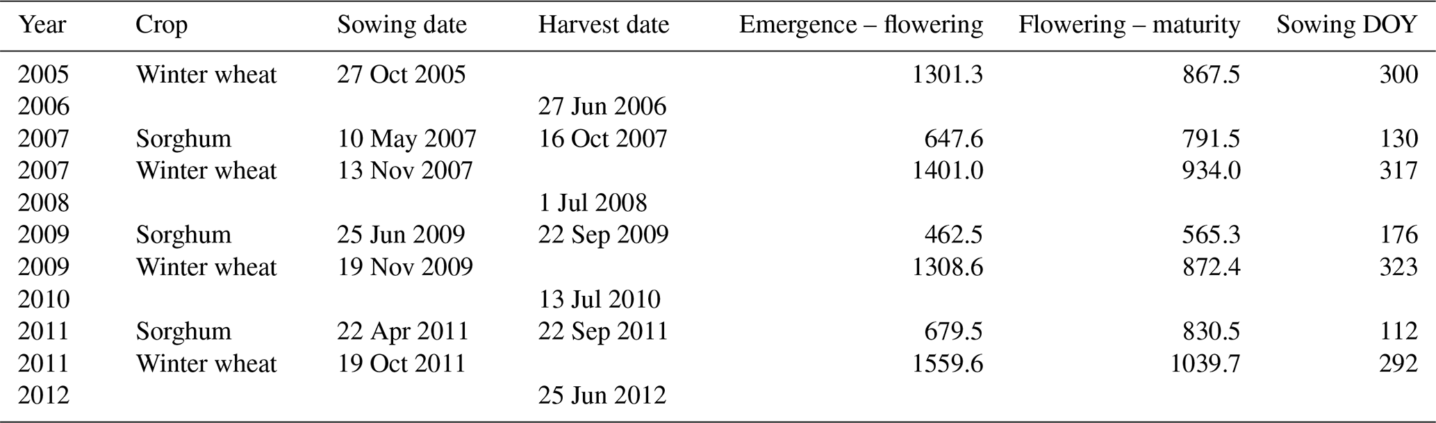
The Avignon “remote sensing and flux site” of the National Research Institute for Agriculture, Food and Environment (INRAE), described in Garrigues et al. (2015a, 2018), provides a well-studied location (Avignon, France 43.917^∘ N 4.878^∘ E) with several years of crop rotation data. The Avignon simulations focus on the period between 2005 and 2013 with a rotation of just two crops: winter wheat and sorghum. JULES already contains parameterizations for wheat and maize. The wheat in JULES is the spring variety which is similar to the winter wheat crop that is grown in Avignon. Spring wheat does not require a vernalization period, which is a process usually needed for winter wheat varieties to achieve optimum yields (Griffiths et al., 1985; Robertson et al., 1996; Mathison et al., 2018). Vernalization is not explicitly implemented in JULES; therefore, spring and winter wheat can be simulated interchangeably. The maize crop is a C₄ crop that is similar to sorghum. Therefore, we use these existing parameterizations rather than develop new ones. During this period, two varieties of sorghum were cultivated. In 2009, a fodder crop variety was grown, with a shorter growing season and a larger LAI than the variety for the other two years (2007 and 2011). Therefore, the 2009 sorghum crop is planted much later in the year compared to the other two sorghum seasons (2007 and 2011) but harvested at a similar time. The aim of simulating the crops at this site is to demonstrate the new sequential cropping functionality in JULES and show how the implementation of sequential cropping affects the JULES crops simulated. The length and detail of the observation record at the Avignon site indicate that it is an ideal site to demonstrate the method being implemented in JULES for simulating sequential cropping. High-resolution meteorological data, important for the practicalities of running the JULES model, are used to run the model using a half-hourly time step; this includes air temperature, humidity, wind speed, rainfall, radiation measurements and atmospheric pressure at a height of 2 m above the surface (Garrigues et al., 2015a, 2018). Irrigation in Avignon is only applied to the summer crops, i.e. sorghum. The observed irrigation amounts are added to the precipitation driving data at the exact day and time they were applied to the crops (Garrigues et al., 2015a, 2018). The irrigation and other settings governing irrigation are therefore not switched on in JULES for the Avignon site simulations (Table 1, column “Avignon settings”). We include simulations for the Avignon site where the crops are represented by grasses (Avi-grass) for comparison with the simulations that use the JULES-crop model. In the Avi-grass simulations, the LAI and the canopy height are prescribed from observations in order to capture the growing seasons correctly without the crop model, and the PFT parameters are adjusted to be the same as the crops. These Avi-grass simulations use the same photosynthesis and respiration calculation as JULES-crop, but this is not allowed to influence LAI as they do in the crop model. This allows the evaluation of the photosynthesis and respiration parts of the model, together with the water and energy fluxes, when the observed LAI and canopy height are used. In the Avi-grass simulations, JULES is not modelling the crops as grasses but fixing some parts of the crops (LAI and canopy height) straight to observations. We also run two simulations that use the crop model: a single-crop (Avi-single) and a sequential-crop simulation (Avi-sequential). In both the Avi-single and Avi-sequential simulations, the LAI and the canopy height are calculated by the model. The JULES total aboveground biomass is calculated from the sum of the stem, leaf and harvest carbon pools for each crop. Observed sowing and harvest dates from Garrigues et al. (2015a) are used to calculate the thermal time requirements for each crop represented in the simulations; these are provided in Table 4. During the periods between each crop, the ground is mostly bare (Garrigues et al., 2018). The only difference between the Avi-sequential and Avi-single simulations is that Avi-single only simulates wheat; therefore, no sowing dates are provided for sorghum.

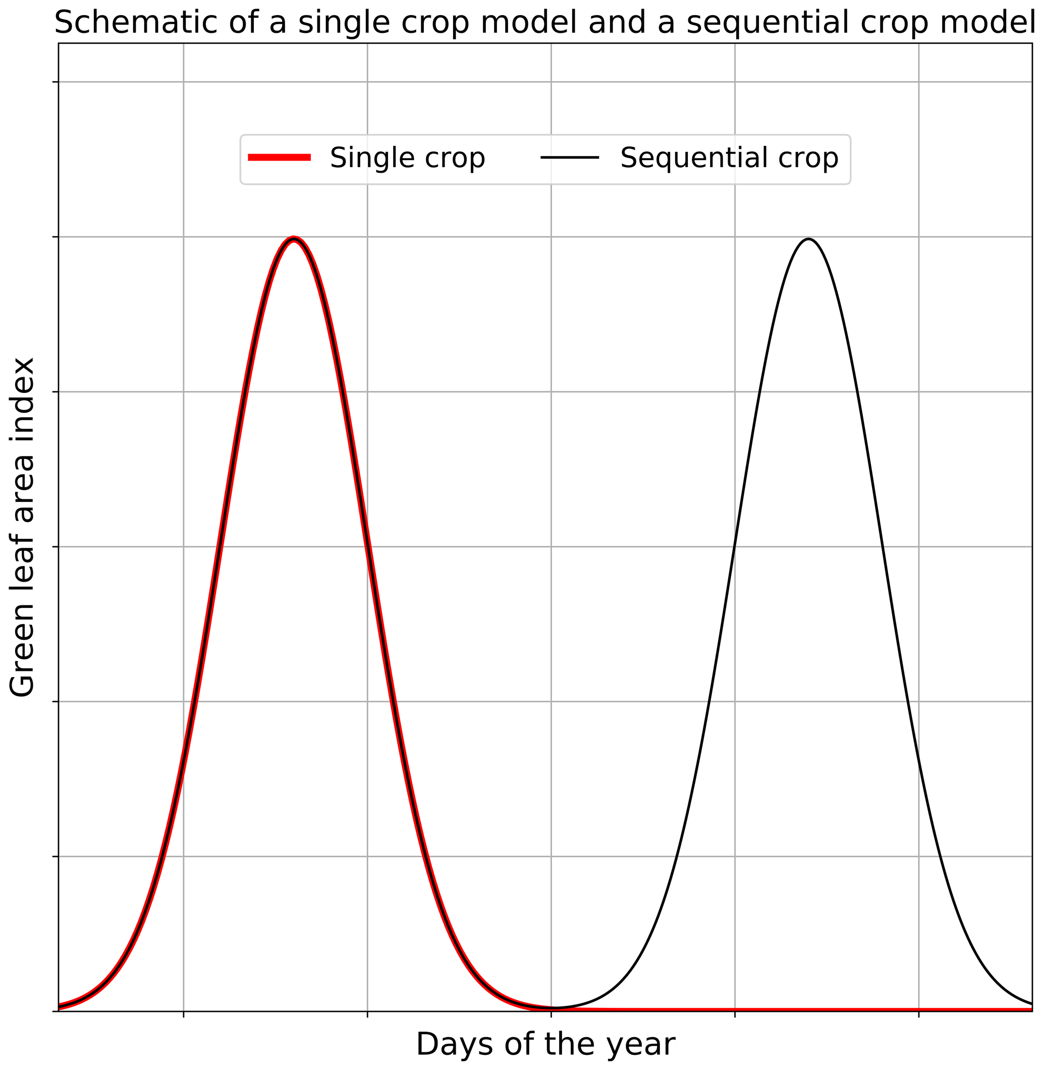
Figure 1 A schematic describing the single-crop model (red curve) that is part of the standard JULES-crop and the new option for including sequential cropping (black curve). This schematic represents a generic crop at a single location.

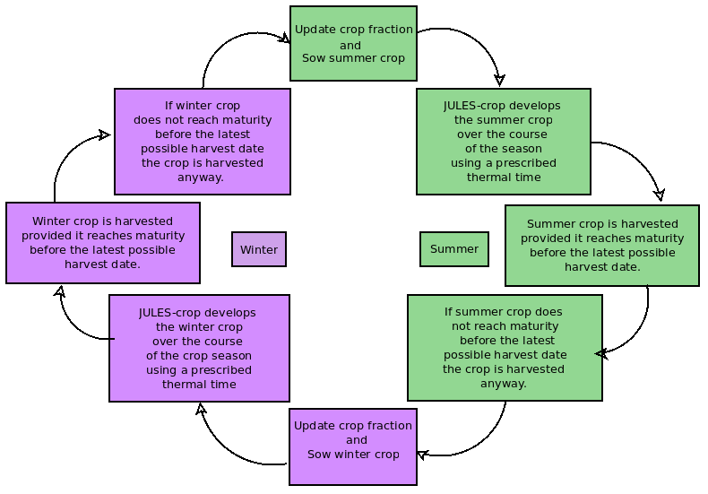
Figure 2 A flowchart showing the sequence followed to carry out the crop rotation in JULES. The first step (top green box) in the sequence is to update the first crop fraction; this occurs as or just before the first crop is sown.

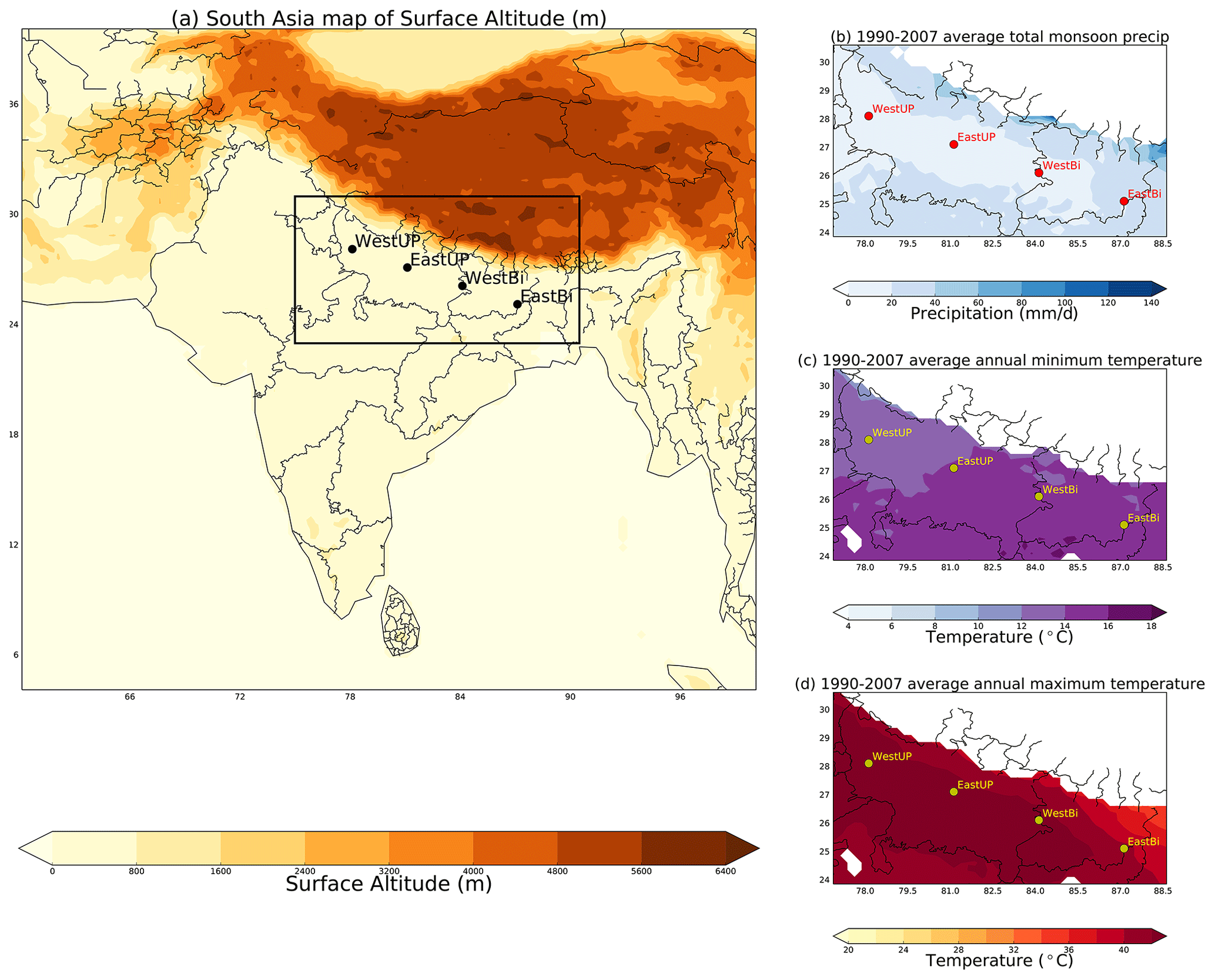
Figure 3 A map showing the location of the single-grid-box simulations in the wider context of India on a map of the surface altitude (a) from the regional climate model that is used in the JULES simulations. The same locations are shown in three smaller maps (b–d) that zoom in on the states of Uttar Pradesh and Bihar. The map in panel (b) shows the total monsoon precipitation, (c) shows the minimum temperature, and (d) shows the maximum temperature averaged for the period 1991–2007.

Table 4 Thermal times in degree days used in this study for the Avignon site; these are based on the observed sowing and harvest dates from Garrigues et al. (2015a).

3.2 Uttar Pradesh and Bihar, India, simulations

The India simulations focus on the northern Indian states of Uttar Pradesh and Bihar. These states are key producers of rice and wheat in South Asia and use a regular rice–wheat rotation that is prevalent in this part of India (Mahajan and Gupta, 2009). We include single-grid-box simulations and a regional simulation. The single-grid-box simulations are a selection of four locations from across these two states. For each grid box, both single-crop (referred to as India-single) and sequential-crop (referred to as India-sequential) simulations are run. India-single and India-sequential are set up in the same way, with the only difference being that sowing dates are provided for just one crop. For consistency with the rest of the simulations, only wheat is simulated in India-single. The single-grid-box simulations enable a similar analysis to that described for Avignon (Sect. 3.1), while the regional simulation (this is only a sequential-crop run) is a demonstration of the sequential cropping method being used at larger scales. For the regional simulation, we assume that wheat and rice are grown in every grid box across the two states and the crops are not limited by nutrient availability. The sequential cropping system in this region involves growing rice during the wet monsoon months and an irrigated wheat crop during the dry winter. In these simulations (both single grid box and regional), wheat is only irrigated during its growing period and without applying limits due to water availability (this is referred to as unlimited irrigation). The wheat variety grown in India is spring wheat, which is the standard variety represented by JULES (Sect. 3.1).

The locations of the selected grid boxes are shown on a map of the surface altitude for South Asia in Fig. 3a. The driving data used for these four simulations are from an RCM simulation run for South Asia for the period 1991–2007 as described below. Figure 3b, c and d show a close-up view of the locations selected. The map in Fig. 3b shows the average total monsoon precipitation for the 1991–2007 period, while Fig. 3c and d show the average minimum and maximum temperatures, respectively, to illustrate that these four grid boxes are representative of the climate of the wider Uttar Pradesh/Bihar region.

In both the single-grid-box and regional India simulations, JULES is run using a 3-hourly time step using driving data from ERA-Interim (Dee et al., 2011; Simmons et al., 2007) downscaled to 25 km using the HadRM3 RCM (Jones et al., 2004). This RCM simulation is one of an ensemble of simulations produced for the EU-HighNoon FP7 project for the entire Indian subcontinent (25–32^∘ N, 79–88^∘ E). The HighNoon simulations are described in detail in previous publications such as Kumar et al. (2013) and Mathison et al. (2013, 2015). HadRM3 provides more regional details in addition to the global data with updated 3-hourly lateral atmospheric boundary conditions interpolated to a 150 s time step. These simulations include a detailed representation of the land surface in the form of version 2.2 of the Met Office Surface Exchange Scheme (MOSESv2.2; Essery et al., 2001). JULES has been developed from the MOSESv2.2 land-surface scheme, and therefore the treatment of different surface types is consistent between the RCM and JULES (Essery et al., 2001; Mathison et al., 2015). In the India single-grid-box simulations, sowing dates are prescribed using climatologies calculated from the observed dataset (Bodh et al., 2015) from the government of India, Ministry of Agriculture and Farmers Welfare. Thermal times are calculated using these climatological sowing and harvest dates from Bodh et al. (2015) and a thermal climatology from the model simulation as described in Osborne et al. (2015); the values used in the simulations here are provided in Table 5. In the regional simulation, the thermal time requirements are estimated from the sowing and harvest dates provided by the Mathison et al. (2018) method to avoid problems with missing observed data. The settings used for the India simulations are provided in Table 1 (column “India settings”). Plots of the regional ancillaries for each of rice and wheat are provided in Appendix C.

Table 5 The sowing day of year (sowing DOY) and thermal times in degree days used in this study for the locations in Uttar Pradesh and Bihar, India (Fig. 3 for a map of the locations), the values given here are based on the observed sowing and harvest dates from Bodh et al. (2015).

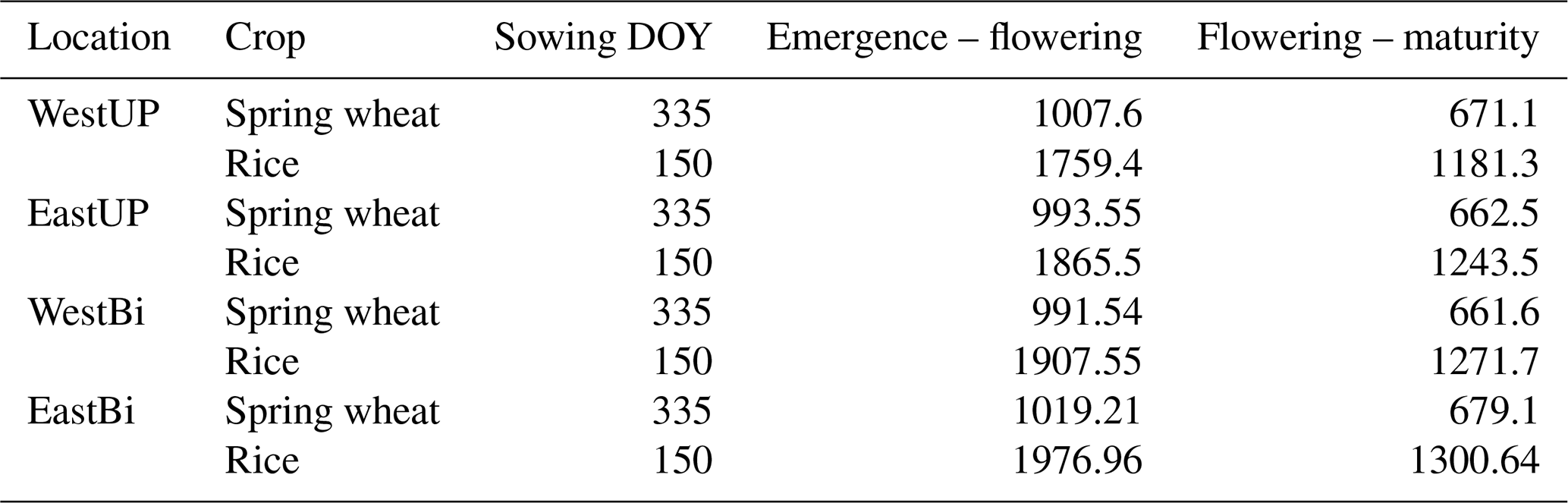
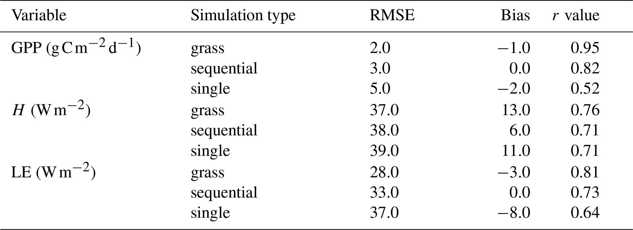
Table 6 Table of statistics comparing the Avignon simulations with observations for each type of run: Avi-single (single), Avi-sequential (sequential) and Avi-grass (without the crop model).

4 Model evaluation

The objectives of this study are to evaluate the model against observations where they are available, for the Avignon point and the India single-grid-box simulations, and to test the following hypotheses with regard to the implementation of the presented sequential cropping method in JULES:

1. Null hypothesis: the inclusion of a secondary crop on the same field does not change the growth and development of the primary crop in an irregular sequential cropping rotation with long fallow periods.
   Alternative hypothesis: the inclusion of a secondary crop on the same field modifies the growth and development of the primary crop in an irregular sequential cropping rotation with long fallow periods.

2. Null hypothesis: the inclusion of a secondary crop on the same field does not change the energy and carbon fluxes in an irregular sequential cropping rotation with long fallow periods.
   Alternative hypothesis: the inclusion of a secondary crop on the same field modifies the energy and carbon fluxes in an irregular sequential cropping rotation with long fallow periods.

3. Null hypothesis: in a regular rotation without long fallow periods, the inclusion of a secondary crop on the same field does not change the crop development of the primary crop or the grid box energy and carbon fluxes and soil conditions.
   Alternative hypothesis: in a regular rotation without long fallow periods, the inclusion of a secondary crop on the same field modifies the crop development of the primary crop, the grid box energy and carbon fluxes and soil conditions.

The first set of hypotheses will be assessed by comparison of the observed LAI, canopy height and total aboveground biomass in Avignon with single-crop and sequential-crop simulations. The second set of hypotheses will be assessed by comparison of observed fluxes, GPP, latent heat (LE) and sensible heat (H) in Avignon with single-crop and sequential-crop simulations. For the third set of hypotheses, we compare JULES yields with observed yields for single- and sequential-crop simulations and analyse the same variables as for the first and second sets of hypotheses for four locations across the northern Indian states of Uttar Pradesh and Bihar. We also assess if the implementation of sequential crops affects the soil moisture in a regular sequential-crop system, which does not have long periods of bare soil. For a regular sequential-crop system without long fallow periods, changes in soil moisture are more likely to be due to the effects of sequential cropping and are less likely to be affected by evaporation from bare soil. More information is provided about the Avignon site in Sect. 4.1 and the climate across the four India grid box locations in Sect. 4.2, including the observations used to evaluate the simulations at these locations.

4.1 Avignon

Avignon is characterized by a Mediterranean climate with a mean annual temperature of 287.15 K (14 ^∘C) and most rainfall falling in autumn (with an annual average of 687 mm). The Avignon time series of temperature (with a 10 d smoothing applied) is provided in Appendix A in Fig. A1a and precipitation (10 d totals, which include actual irrigation amounts) in Fig. A1b (Garrigues et al., 2015a). In general, Avignon experiences a fairly regular distribution of rainfall throughout the year and the annual temperature range for Avignon (26 ^∘C) is relatively consistent, with only a brief cold snap in early 2012 having a much lower minimum. The Avignon site represents the irregular cropping rotation, chosen because it has been observed and documented over several years (2001 to 2014), growing a range of crops throughout this period. No equivalent site to Avignon has been found for South Asia.

The observations for evaluating the model include canopy height (measured every 10 d), aboveground dry weight biomass (taken at four field locations) and LAI; biomass and LAI are destructive measurements repeated up to six times per crop cycle (Garrigues et al., 2015a). H and LE flux measurements are available for several years, enabling the evaluation of the JULES fluxes. Cumulative evapotranspiration (ET) are derived from the half-hourly LE measurements. More information is documented in Garrigues et al. (2015a) regarding the site and the observations available. These continuous measurements of surface fluxes provided by the Avignon dataset are a unique resource for evaluating LSMs and for testing and implementing more irregular crop rotations in LSMs.

4.2 India

The four India locations (grid boxes) selected for analysis in this study are shown on a map of South Asia in Fig. 3a with smaller inset plots (Fig. 3b, c and d) focusing on the sequential cropping region being considered across the states of Uttar Pradesh and Bihar. The climate of this region is summarized in Appendix B (Fig. B1), which shows the time series of the average precipitation (Fig. B1a), temperatures (Fig. B1b) and vapour pressure deficit (VPD) (Fig. B1c) at each of these four grid boxes. The different crop seasons are emphasized by the different colour shading, with yellow for wheat and pink for rice. The temperatures (Fig. B1b) rarely reach the lower cardinal temperatures set in the model (T_b) shown for rice (green) or wheat (orange); however, the high temperatures do exceed the maximum cardinal temperatures (T_m) for these crops, especially those set for wheat. In general, EastBi is cooler than the other locations in more of the years, with the two locations in Uttar Pradesh often being the warmest. The precipitation at each location is variable (Fig. B1a), with variation in the distribution of precipitation through the monsoon period, which could be important for crop yields. Challinor et al. (2004), for example, found that in two seasons with similar rainfall totals, the distribution of the rainfall during the growing season strongly affected groundnut crop yield. There is also a clear seasonal cycle in the VPD, increasing toward the end of the wheat season and decreasing into the rice season. EastBi generally has the lowest VPD, with WestUP and EastUP usually the highest throughout the time series shown (Fig. B1). These time series show that there is a gradual change in conditions from west to east across Uttar Pradesh and Bihar with increasing humidity and rainfall and decreasing maximum temperatures from west to east.

District-level area and production data from the International Crops Research Institute for the Semi-Arid Tropics (ICRISAT, 2015) are used to calculate district level yields. These are then gridded at the resolution of the ERA-Interim data (0.25^∘) to ensure that the scale of simulated and observed yields matched. We also show average crop yield observations for three 5-year periods (Ray et al., 2012a) between 1993 and 2007 (1993–1997, 1997–2003, 2003–2007). Data from Ray et al. (2012a) are made available via Ray et al. (2012b). Ray et al. (2012b) are based on previous publications (Monfreda et al., 2008; Ramankutty et al., 2008). All the observations used include the period of the single-grid-box simulations, which are from the period of 1991–2007. We show both of these datasets to highlight that there is a range in the estimates of yield for this region.

5 Results

5.1 Evaluation against observations

5.1.1 Avignon

Figure 4 shows the time series of total aboveground biomass (a), LAI (b) and canopy height (c) for Avi-sequential and Avi-single compared with observations. The crops in JULES (both single and sequential) are developing throughout the crop seasons, with maxima occurring at approximately the correct time for the crops being simulated. Therefore, the lack of vernalization in the model does not affect the simulation of winter wheat in Avignon. Avi-grass simulations are not shown, as these follow the observed canopy height and LAI exactly as these values are prescribed in the simulations without crops. The total aboveground biomass from JULES is plotted as a time series (dashed lines) for comparison with observations, which are provided as a single time series with the crop type confirmed from the timing of the observations (purple asterisks in Fig. 4a). The increase in biomass for both crops through the start of the season follows the observations quite closely but in most years, especially for wheat, JULES-crop (using either single or sequential crops) does not accumulate enough biomass later in the crop season to reach the observed maxima. The wheat canopy height is very close to observations for all four seasons; however, the wheat LAI is overestimated. The two wheat seasons of 2006 and 2010 are closer to the LAI observations than 2008 and 2012, but the underestimation of the biomass is greater for these seasons. Garrigues et al. (2015a) highlight that 2006 and 2008 have atypical rainfall during the wheat season, with 2006 being very dry (256 mm of rain during the wheat season) and 2008 being very wet (500 mm during the wheat season). Therefore, in 2008, Avignon received 73 % of its annual average (Sect. 4.1) during the wheat season alone; these differing conditions could explain the large differences in observed LAI and biomass between the two years (Garrigues et al., 2015a).

The shorter observed growing season for the taller fodder variety of sorghum grown in 2009 can be compared with the longer season, smaller variety grown in 2007 and 2011 (solid red line Fig. 4b and c). No sorghum is simulated in Avi-single, so the dotted red line is equal to zero and not visible in Fig. 4. Avi-sequential (dashed red) simulates the 2009 sorghum season well, in terms of biomass (Fig. 4a), LAI (Fig. 4b) and canopy height (Fig. 4c); with relatively small differences between the simulations and observations maximum values (LAI of 1 m² m⁻² and canopy height of 0.1 m). In the 2007 sorghum season, Avi-sequential (dashed red) overestimates the maximum LAI and canopy height by approximately 2 times the observations (Fig. 4b and c) and underestimates the total biomass (Fig. 4a) by about 30 %. For the 2011 season, the Avi-sequential sorghum biomass is equal to the magnitude of the observations; however, the maximum LAI is overestimated by a factor of 4 in the model (similar to 2007) and the maximum canopy height is approximately 2 times the observed maximum.

The peaks in productivity shown in the LAI in Fig. 4b are consistent with the two years (2006 and 2007) of GPP observations (black line Fig. 5a). The 2006 wheat crop is represented in the GPP of all three simulations, although it is underestimated in all of them (Fig. 5a). The GPP in Avi-single is lower than both Avi-sequential and Avi-grass during the second half of the wheat growing period. The decline in GPP at the end of the 2006 wheat season is quite close to the observations for the three simulations, with Avi-grass (red line) being slightly early and both the crop simulations; Avi-sequential (blue line) and Avi-single (cyan line) being slightly late. For the sorghum growing period, the magnitude and timing of the maximum GPP for Avi-sequential (blue line) are a good fit to observations. However, the increase in GPP begins slightly too early for Avi-sequential and slightly late for Avi-grass. The Avi-grass simulations slightly underestimate the maximum GPP during the sorghum season and it occurs a little later than observed (Fig. 5a). The decline in GPP at the end of the sorghum season occurs at the same time as the observations for both Avi-grass and Avi-sequential. These results are quantified in Fig. A3, with both Avi-grass (Fig. A3a) and Avi-sequential (Fig. A3b) showing a strong linear correlation, with r values greater than 0.8. The values for Avi-single (Fig. A3c) are lower, with an r value of approximately 0.5; this is because the observations contain seasons with both sorghum and wheat, which is not possible in Avi-single. The statistics discussed here are summarized in the GPP row of Table 6). It is likely that the representation of both crops in Avignon in terms of the crop growth and development would be improved by developing specific crop parameterizations for winter wheat and sorghum in JULES.

Comparisons between the simulated energy fluxes (H and LE) and observations are shown in Figs. A2 and A3d–i. The RMSE and bias values for H and LE are given in Table 6; these are generally comparable to those from Table 5 in Garrigues et al. (2015a), which are LE: RMSE of 52.4 W m⁻², bias of −11.8 W m⁻²; and H: RMSE of 56.2 W m⁻², bias of 17.6 W m⁻². The linear correlations for H are strong for all three simulations, with r values above 0.7 (Avi-grass, Fig. A3d; Avi-sequential, Fig. A3e; and Avi-single, Fig. A3f). The linear correlations for LE are more variable between the three simulations, with Avi-grass (Fig. A3g) having the strongest correlation (r value of 0.81), Avi-single (Fig. A3i) having the weakest correlation (r value of 0.64) and Avi-sequential (Fig. A3h) in between the two (r value of 0.73). The H values for all three simulations and the LE values for Avi-grass and Avi-sequential are comparable to but lower than those from Table 5 in Garrigues et al. (2015a), which provides correlation values of 0.8 for LE and 0.85 for H. The annual cycles of LE and H are shown in Fig. A2a and b, respectively. Generally, the seasonal cycles of H and LE are captured well in JULES (Fig. A2 and the time series in Fig. 5b and c). The annual cycle for LE is close to observations in the first half of the year but too high in the second half for Avi-grass and Avi-sequential. Avi-single is much too low, which explains its lower r value. Overall, H is closer to observations for all three simulations; however, the annual cycles show that both Avi-grass and Avi-single are a little too high and similarly Avi-sequential a little too low, explaining why the r values for this variable were much closer to each other.

5.1.2 India

The water resource requirement of a crop is affected by the size of the crop and its leaf area with overestimation (underestimation) of these characteristics potentially skewing the results towards a higher (lower) resource requirement. Canopy heights for both the regional simulation and the single-grid-box simulations for both rice and wheat across the region are between 0.5 and 0.7 m (not shown), which is an expected value for a typical crop, as described in Penning de Vries et al. (1989). Similarly, LAIs in both the regional and single-grid-box simulations are consistent with each other. Figure B3 shows the LAI for each of the four single-grid-box simulations. This shows that wheat LAI from JULES is between 5 and 7 m² m⁻² across the locations; this is also an expected value for a crop according to Penning de Vries et al. (1989). Rice LAI is lower (between 2 and 4 m² m⁻²), with the lowest values for WestUP, slightly increasing from west to east locations. For WestUP particularly, rice (solid red line) has a small LAI (Fig. B3) but it generates a yield (red asterisks in Fig. B2) that falls within the range of the observations for each year. However, wheat (solid black line) generates an LAI that is closer to expected values but a smaller yield compared with observations (Fig. B2, black asterisks). The inclusion of both observation datasets in Fig. B2 highlights the spread between yield estimates for this region.

Figure 6 shows single-grid-box yields for both the India-single (asterisks) and India-sequential (circles), illustrating that the wheat crops simulated in both India-single and India-sequential are very similar to each other. Figure 6 compares the JULES yields with observed yields from ICRISAT (2015), indicating that the yields change at each of the locations from west to east. However, comparisons with observed yields should not be overinterpreted because the combined stresses that will be implicit in the observations, such as nutrient and water stress are not accounted for in these simulations. We also assume that rice and wheat are grown in rotation everywhere, which will be an overestimation. The observed yields, particularly for wheat are larger to the west and reduce to the east (shown for the whole region for rice – Fig. C3a; and wheat – Fig. C3c). In both the India-single and India-sequential crop simulations, JULES simulates a reduction in wheat yields from west to east; however, this is not as extreme in the simulations as it is in the observations because JULES tends to underestimate the wheat yield especially for the western locations. Across both observation datasets, the bias is smaller for the other locations, with rice and wheat yields within the range of the observations for most years (Fig. B2). For EastBi, the rice yields are often toward the top of the range provided by the two observed datasets but still within the range of the observations (Fig. B2). The spatial distributions of JULES rice and wheat yields from the regional simulation are shown in Fig. C3 and reflect the results shown in the single-grid-box simulations.

5.2 Crop growth and development

5.2.1 Avignon

Figure 4 shows that there are only small differences between Avi-single (dotted line) and Avi-sequential (dashed), particularly for total aboveground biomass (Fig. 4a) and canopy height (Fig. 4c). The LAI in JULES is typically more sensitive to changes in conditions than the biomass or canopy height, but even these differences between Avi-single and Avi-sequential LAI are small. The observations show that there was a sorghum crop during the summer immediately before the 2008 and 2012 wheat crop; during these years, the LAI of Avi-single is slightly larger than that of the Avi-sequential and observations. In Avi-single, this sorghum crop is not present, which could affect the condition of the soils in the model at the time the wheat is sown. Overall, Fig. 4 shows that a similar wheat crop is simulated in both the single- and sequential-crop simulations, which is expected because both use the same parameterization to calculate crop development. Including a secondary crop on the same field in Avi-sequential does not really affect the primary crop growth and development, which means that Avi-single and Avi-sequential simulate a very similar primary (wheat) crop.

5.2.2 India single-grid-box simulations

The LAI in Fig. B3 together with the yields in Fig. 6 show that the wheat crop in India-sequential is indistinguishable from the wheat crop in India-single. The canopy height is very similar to the LAI; therefore, it is not shown here. In each of the figures showing LAI and yield, it is only occasionally possible to see the two simulations, highlighting that the crop growth and development of the primary crop is not really changed by the implementation of a secondary crop at the same location in JULES.

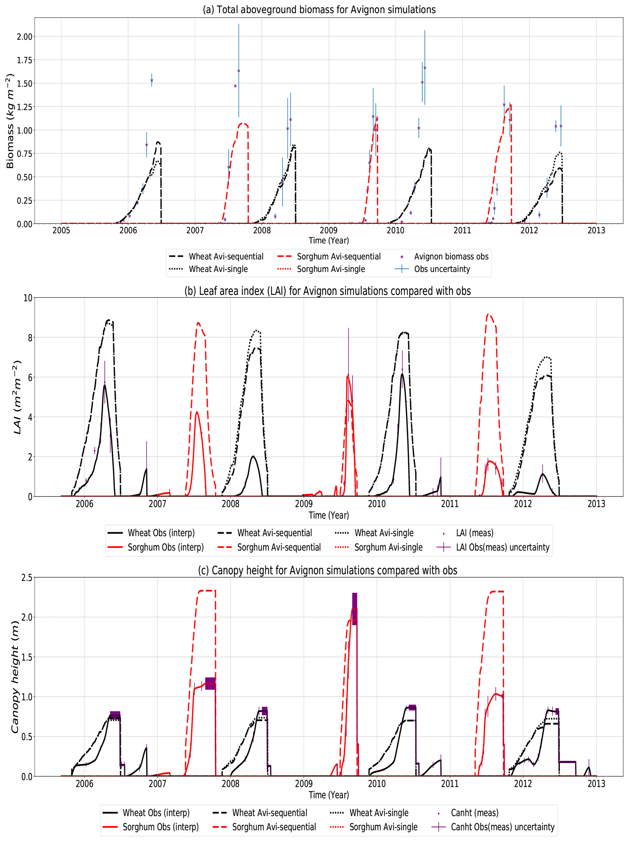
Figure 4 Time series of total aboveground biomass (a), LAI (b) and canopy height (c) for the Avignon site for wheat (black) and sorghum (red) for observations (solid lines) and simulations using the observed sowing and harvest dates: Avi-sequential (dashed) and the wheat-only Avi-single (dotted) simulations for the period between 2005 and 2013 using observed sowing and harvest dates. Simulations with prescribed LAI and canopy height are not shown here as these follow the observed LAI and canopy height. The dotted red sorghum line in the Avi-single simulation is not visible because this is at zero for the wheat-only simulation. Observed aboveground biomass in panel (a) is shown by purple asterisks. The standard deviation of the measurements is shown to represent the uncertainty in the observations.

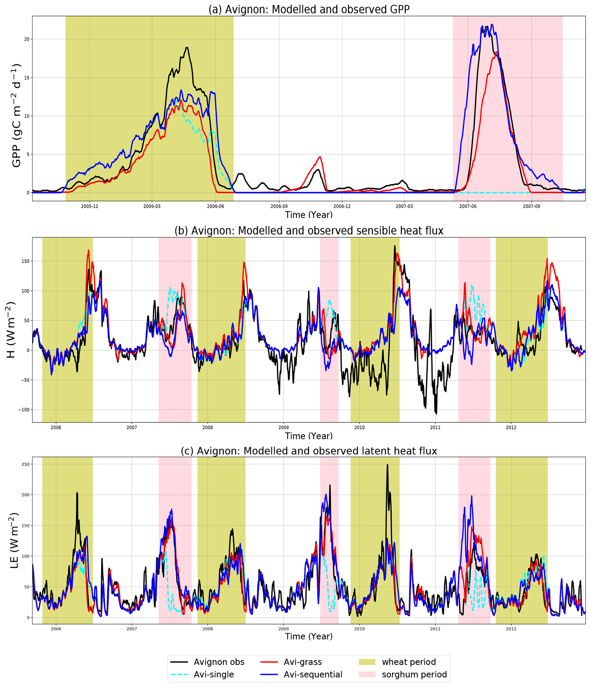
Figure 5 Time series of GPP (a), H (b) and LE (c) for the Avignon site compared with observations (black lines). For H (b) and LE (c), the whole period from 2005 to 2012 is shown, while GPP (a) shows the period 2005–2007 due to availability of observations. In the GPP plot, only one complete winter wheat (yellow) and one complete sorghum season (pink) are highlighted. The following model simulations are also shown: Avi-grass (red), Avi-sequential (blue) and a wheat-only Avi-single (cyan). In each plot, a 10 d smoothing has been applied to the daily data.

Figure 6 Scatter plot comparing the observed rice and wheat yields (ICRISAT, 2015) against JULES simulations at each of the India locations shown in Fig. 3, with India-sequential shown by circles (rice in red and wheat in black). India-single shown by asterisks (rice shown in red and wheat shown in blue). Note that the simulations assume that rice and wheat are grown everywhere and the crops are not limited by pests and diseases or nutrient availability, which will affect the comparison with the observations that implicitly include these aspects.

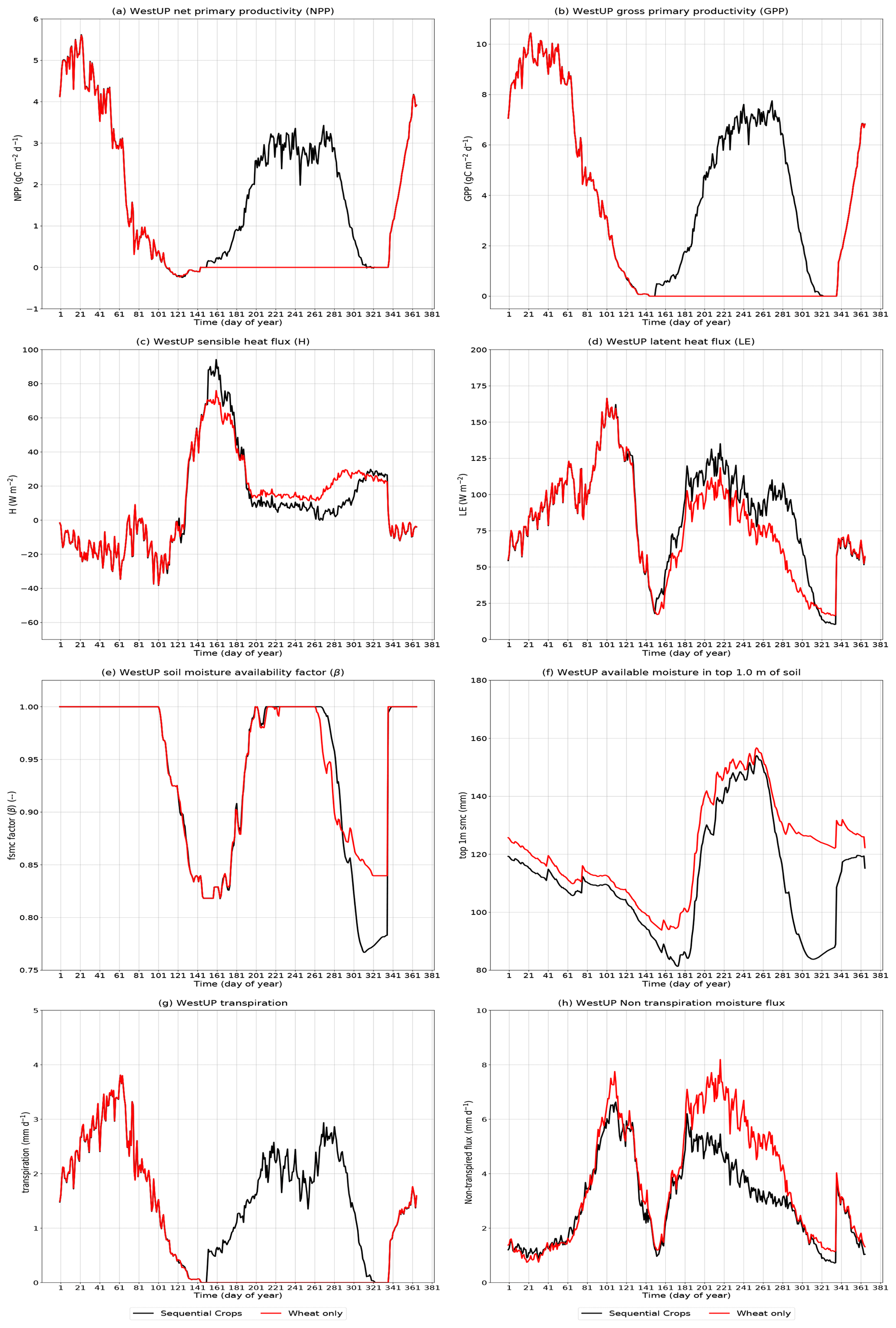
Figure 7 Annual climatology of fluxes (in day of year) for WestUP for India-sequential (black) and India-single (red): carbon fluxes: NPP (a) and GPP (b). Heat fluxes: sensible heat H (c) and latent heat LE (d). Soil moisture variables: β (e) and soil moisture availability in the top 1 m of soil (f). Moisture fluxes: evapotranspiration (g) and non-evapotranspiration moisture fluxes (h).

5.3 Energy and carbon fluxes

5.3.1 Avignon

The time series of GPP (Fig. 5a) shows that all three simulations largely follow each other closely (Avi-sequential, blue line; Avi-single, cyan line; Avi-grass, red line), except during the sorghum growing period, which is not represented using the single-crop version of JULES. During the sorghum season, the land cover in JULES is therefore represented by bare soil, so the GPP goes to zero (dashed cyan line in Fig. 5a). The wheat season fluxes of H (Fig. 5b) and LE (Fig. 5c) also follow each other closely for all three simulations. However, during the sorghum growing period, the effect on the energy fluxes is more complex, with Avi-single having a lower LE and higher H than Avi-sequential and Avi-grass. In Avi-grass and Avi-sequential, it is possible to include representation of the two observed crops and therefore represent the actual land cover at the Avignon site; this is not possible in Avi-single. The inclusion of this secondary crop on the same field in Avi-sequential modifies the energy and carbon fluxes for the part of the year the secondary crop is being represented but the primary crop fluxes remain similar to those in Avi-single.

5.3.2 India single-grid-box simulations

Wheat is simulated in both India-single and India-sequential; it is grown during the last 25 d of one year and the first 140 d of the following year. The carbon fluxes during the wheat season are very similar in both India-sequential and India-single; these are shown for WestUP GPP in Fig. 7a and NPP in Fig. 7b and similarly for the other India locations in Appendix B, Figs. B4a–b, B5a–b and B6a–b. The peak for wheat is therefore the first peak shown in NPP (Fig. 7a) and GPP (Fig. 7b). Wheat NPP begins to decline at around day 41 of the year in both India-sequential and India-single, which is quite early in the season and may have a direct impact on the yield. The decline in NPP could be related to the way the carbon is partitioned to different parts of the plant. A short time series of India-sequential showing how carbon is partitioned to the different parts of the plant for wheat (black) and rice (red) is shown in Appendix B (Fig. B7). The allometric coefficients that control the partitioning of carbon to the different parts of the crop in JULES are currently those from Osborne et al. (2015); it is possible that the results could be improved for South Asia if these were tuned to more appropriate values for the crops there. Rice is planted between day 141 and day 330 of a typical year; this is not represented in the India-single simulation; therefore, the NPP and GPP go to zero during the rice season.

Similar to the carbon fluxes, Fig. 7 shows the fluxes of H (Fig. 7c) and LE (Fig. 7d) for WestUP and the other India locations in Appendix B, Figs. B4c–d, B5c–d and B6c–d. At each location, the energy fluxes during the wheat season for both India-sequential and India-single are largely indistinguishable from each other. The main differences in the energy fluxes occur during the rice season, where India-single has a lower LE and higher H than India-sequential. We investigate the changes in LE further, using the evapotranspiration (for WestUP shown in Fig. 7g) and non-evapotranspiration moisture fluxes (for WestUP shown in Fig. 7h). The sequential-crop method affects the individual components of the moisture flux, resulting in a larger component from the evapotranspiration flux and a lower component from non-evapotranspiration fluxes than India-single; this effect is visible across all four India locations (Appendix B, Figs. B4, B5 and B6g and h).

5.4 Soil moisture

The crop rotation in Avignon has long fallow periods between crops, which means that the effect of sequential crops on soil moisture will also be influenced by soil evaporation. The crop rotation in India does not have long fallow periods, which allows analysis of the effects of sequential crops on soil moisture for the India single-grid-box simulations.

5.4.1 India single-grid-box simulations

The effect of sequential crops on the soil moisture availability factor (β, Sect. 3) is similar to the carbon and heat fluxes, with India-sequential and India-single being consistent with each other for the wheat season. Figure 7e shows β for WestUP (β at the other India locations are shown in Appendix B, Figs. B4e, B5e and B6e). β is mainly affected during the secondary growing period (rice) with India-sequential showing a larger decrease in soil moisture availability over a shorter part of the year than India-single (Fig. 7e). Unlike β and the fluxes of carbon and heat, the available soil moisture in the top 1.0 m is affected by sequential cropping throughout the year; this is shown for WestUP in Fig. 7f. The available soil moisture in the top 1.0 m has much larger variations in India-sequential than in India-single even outside the rice season across the four locations, but particularly for the westernmost locations of WestUP (Fig. 7f) and EastUP (Fig. B4f). The effect of sequential crops on the available soil moisture in the top 1.0 m reduces for the more eastern locations of WestBi (Fig. B5f) and EastBi (Fig. B6f).

These moisture fields show that WestUP has the lowest available soil moisture and therefore β value, suggesting this location is likely to be the most water stressed. It is also the western locations that are more affected by the implementation of sequential crops. WestBi, on the other hand, is least affected by the implementation of sequential crops, often with the highest β and the most consistent available soil moisture in the top 1.0 m across the year of the four locations. This is consistent with the temperature and precipitation time series shown in Fig. B1, where the locations to the east are wetter and cooler than those to the west. This means there is more available soil moisture in the top 1.0 m for the eastern locations compared with the western locations.

6 Discussion

The sequential cropping system is used around the world especially in the tropics but is relatively underrepresented in land-surface models and consequently climate simulations. Most crop models are only able to simulate one crop per year, which limits their use in many parts of the world. Often this means that only one of the crops in a rotation are modelled explicitly, with the rest of the year represented by bare or almost bare soil. In a single-crop model, the correct land cover is not represented for the season that is not being simulated, which means that water, carbon and energy fluxes are incorrect for this season. An alternative approach used by ISIMIP (Warszawski et al., 2013, 2014) simulates each crop for a small fraction of each grid box, thereby producing a yield for each crop for each grid box; this is then post-processed to give larger-scale yields. The ISIMIP approach is effective if yields are the primary focus, but it is not applicable for understanding the use of water resources across different seasons. The real benefit of the sequential cropping capability is that it can represent the observed land cover in a single simulation, which improves the simulation of water, energy and carbon fluxes. Including sequential crops enables a continuous simulation for multiple years and seasons, which provides an understanding of the evolving demand for resources.

We present a method for simulating sequential crops in JULES with a view to enabling JULES-crop to represent these cropping systems in Earth system and climate models for application in adaptation and mitigation studies. We demonstrate its use for a site in Avignon, France, which uses the sorghum–winter wheat rotation and the Indian states of Uttar Pradesh and Bihar, where the rice–spring wheat rotation is prevalent. The wheat season is represented in all sequential- and single-crop simulations, producing a similar wheat crop in terms of LAI, canopy height and yield (or as observed in Avignon, total aboveground biomass). This is expected because the sequential-crop method does not change the parameterization of crops in JULES but changes the control of the crop code to allow it to be used more than once per year. This means that the crop growth and development are not affected by the inclusion of sequential cropping in JULES for neither Avignon nor India. For Avignon, there are small differences in the LAI of the single-crop simulation but only for wheat seasons which occur immediately after a sorghum season that is not being represented. These small differences in LAI in Avignon could be due to differences in soil conditions, where sorghum is not being simulated but the irrigation water is still being applied via the precipitation.

The representation of crops, either using the crop model (Avi-sequential) or using grasses (Avi-grass), has a similar effect on the surface fluxes, which shows that the code used by the wider vegetation in JULES as well as the crop model is approximating leaf-level photosynthesis, stomatal conductance, water stress and leaf-to-canopy scaling correctly when compared with observations. For simulations that include both crops (Avi-sequential and Avi-grass), fluxes of carbon and heat are generally captured well for Avignon compared with observations. There are regular differences in the fluxes during the wheat-only single-crop simulations at all locations. The single-crop simulation cannot simulate the correct land cover during the second crop of the rotation; for Avignon, this is the sorghum season, and for India, the rice season. In Avignon, compared with observations, the LE is too low and H is too high during the sorghum season not being explicitly represented in JULES. The surface fluxes for the India grid box simulations are consistent with those in Avignon, with a higher H and lower LE in India-single than in India-sequential. In the sequential simulations, the representation of the land surface is closer to the observed land cover because bare soil and the relevant crops can be reproduced within the simulation when they are typically observed. This analysis shows that the main heat and carbon fluxes are changed by the implementation of sequential cropping, with the main differences occurring during the period where a crop is observed but is not usually represented in the simulation.

The regular rice–wheat rotation across India does not have long periods of bare soil, allowing the effect of sequential crops on soil moisture to be considered. The climate of Uttar Pradesh and Bihar, two of the main producers of rice and wheat in India, is highly variable, both in terms of temperature (ranging from 7 to 52 ^∘C) and rainfall (between 0 and 15 mm d⁻¹). Across these states, there is a cooling moistening trend from west to east, making conditions for growing crops very different across a relatively limited area. In the India-single simulation, the available soil moisture is less variable than the India-sequential simulation; this is not limited to an individual crop season but is evident throughout the year. In general, this increased variability is more pronounced for the more arid western locations, with the wetter eastern locations being less affected. Sequential cropping is therefore modifying the soil moisture availability across all the crop seasons. The aridity of these more westerly locations could be exacerbated by the lack of irrigation in the RCM driving data that prescribe the JULES climate in these simulations. This region is intensively irrigated (Biemans et al., 2013), which means that there is a significant contribution to atmospheric humidity from evaporation due to irrigation and the recycling of water into precipitation (Harding et al., 2013; Tuinenburg et al., 2014) that cannot be accounted for here. Tuinenburg et al. (2014) estimate that as much as 35 % of the evaporation moisture from the Ganges Basin is recycling within the river basin. Therefore, in these simulations, we are missing the part of the water cycle that allows evaporation from the surface to affect the humidity.

WestUP has the least favourable conditions for crops, with the least available soil moisture and higher temperatures than the other locations, yet the observed yields are higher than the eastern locations. The observed yields at EastBi are the lowest of the four locations, where the cooler wetter conditions should be more conducive to achieving higher yields; these are neither observed nor modelled. This is likely to be due to the differing management practices between the two states of Uttar Pradesh and Bihar. Uttar Pradesh is characterized by high agricultural productivity with effective irrigation systems (Kumar et al., 2005) and early adoption of new management practices (Erenstein and Laxmi, 2008). Bihar, on the other hand, has lower agricultural productivity, farms tend to be smaller and more fragmented, irrigation systems are less effective (Laik et al., 2014), and adoption of new technology is also slower due to the lack of available machinery (Erenstein and Laxmi, 2008). Yield gap parameters are included in many crop models in order to account for the impact of differing nutrient levels, pests, diseases and non-optimal management (Challinor et al., 2004), thus explaining the difference between potential and actual yield under the same environment (Fischer, 2015). This is not included in these simulations.

The regional sequential simulation shows that the sequential cropping method presented here can be used at larger scales. From the analysis for Avignon and the four India grid boxes, we anticipate that the inclusion of sequential crops will have a significant impact on the surface fluxes of energy, carbon and soil moisture at regional scales. However, in the simulation presented, it is assumed that crops are grown everywhere across Uttar Pradesh and Bihar. For a fair and comprehensive evaluation of the impacts of sequential crops at regional scales, this simulation requires further development to represent the types of crops, together with where and when they are grown. Future work will compare a regional sequential simulation (based on the larger-scale simulation presented here), with an equivalent single-crop simulation that includes realistic crop fractions, to understand the impact of sequential crops on a regional scale. Irrigation is also important for this region; while this is included in these simulations, it is only applied during the dry wheat season with no irrigation during the monsoon rice season. Some irrigation may also occur during monsoon breaks if there is a significant drop in soil moisture; this would be a useful future JULES development. Future developments to include the effects of heat stress, soil nutrient limitations, pests and diseases on crops in JULES would also be useful. The simulations shown here consider a small number of rotations, crops and regions. However, different varieties and types of crops, the timing of sowing and harvesting, together with many possible irrigation options, can have a large impact on the model results. This is an important consideration for future work and should be investigated fully when applying this method to new areas.

7 Conclusions

In this paper, we describe and implement a new sequential cropping capability in JULES enabling more than one crop to be simulated at a given location during a growing season (available in JULES from version 5.7). This is another step towards being able to include JULES-crop in Earth system and climate models, allowing more accurate representation of land use and surface coverage in regions where two or more crops are grown in rotation. This is important for accurate representation of the fluxes of carbon and energy in climate simulations in regions with more than one crop grown in one location within a year. Sequential crops reduce H and increase LE, thereby modifying the contribution from the different components of the latent heat flux. For crop rotations without long fallow periods, including sequential crops also affects the availability of soil moisture throughout the year. More realistic fluxes of carbon, water and energy are important for understanding the impacts of climate change. The continuous simulation of all crops throughout the year also provides a more complete picture of the total demand for water resources, which is important for climate impact assessments. We show that JULES simulates two realistic crops in a growing season both in Avignon (wheat and sorghum) and across Uttar Pradesh and Bihar (rice and wheat). For Avignon and India, the maxima of LAI, canopy height and biomass (yield) occur at approximately the correct times of the year. For Avignon, the observed GPP and energy (H and LE) fluxes are reproduced, correlating well with observations. There are only small differences between using the crop model and using grasses to represent the crops at this site, indicating that JULES-crop can reproduce the LAI and canopy height well enough to compare well with the observed surface fluxes. The representation of crops in Avignon could be improved by including crop-specific parameterizations of winter wheat and sorghum in the model, although sorghum would probably require two different sets of parameters for a significant improvement because the two varieties grown at the site are so different.

A regional simulation provides the basis for future sequential-crop simulations for a larger area. This cropping system is likely to be a feature of the future land surface, not just in the tropics but globally as an adaptation to climate change. Therefore, we encourage other modelling communities to include sequential crops in their models, so that it can benefit from being part of future model intercomparison projects such as AgMIP (Rivington and Koo, 2010; Rosenzweig et al., 2013, 2014) and ISIMIP (Warszawski et al., 2013, 2014) and be developed further.

Appendix A: Avignon comparison

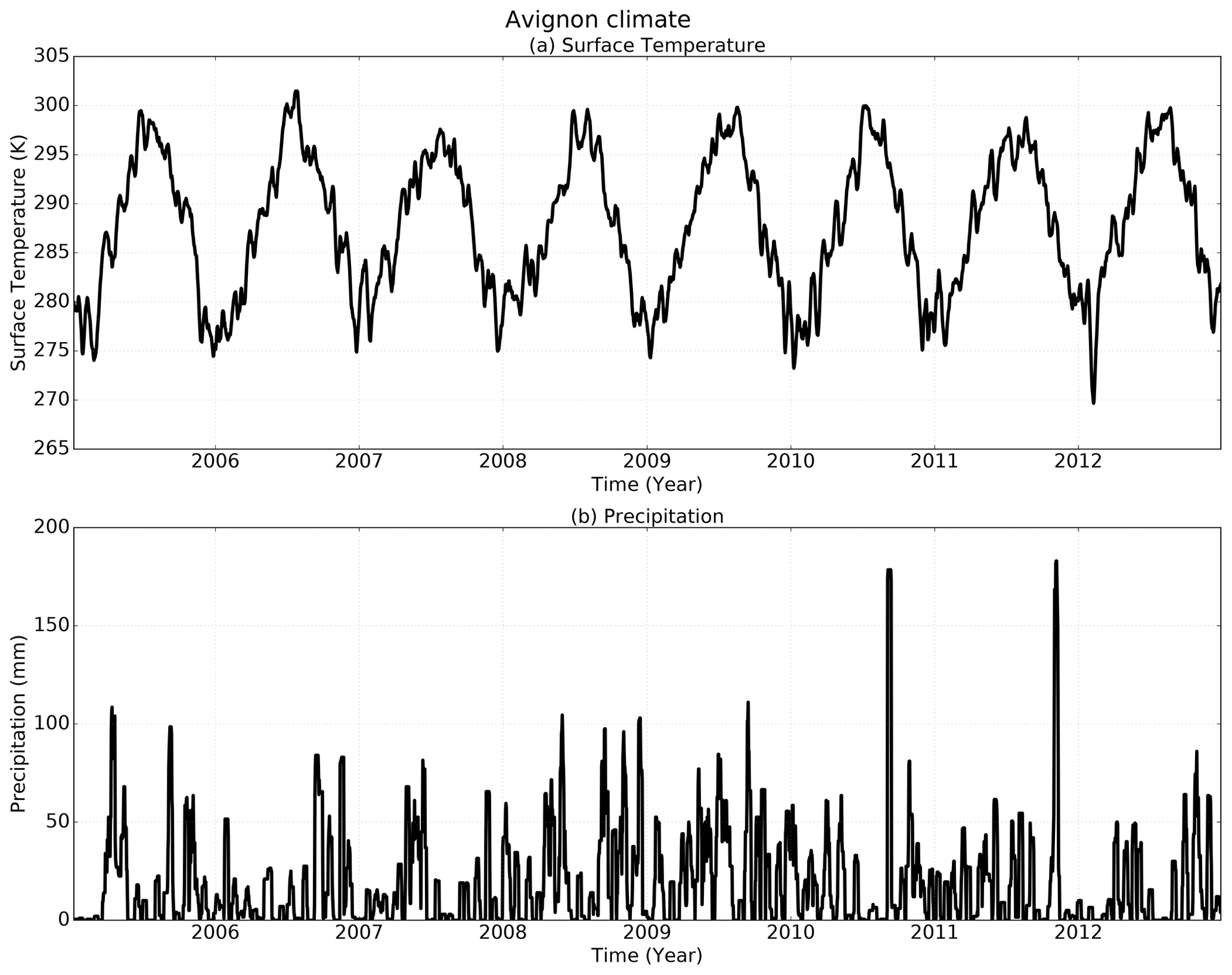
Figure A1 Time series of temperature (a) and precipitation which includes the observed irrigation amounts added at the exact day and time they were applied to the crops (b) in Avignon for the time period analysed (2005–2012).

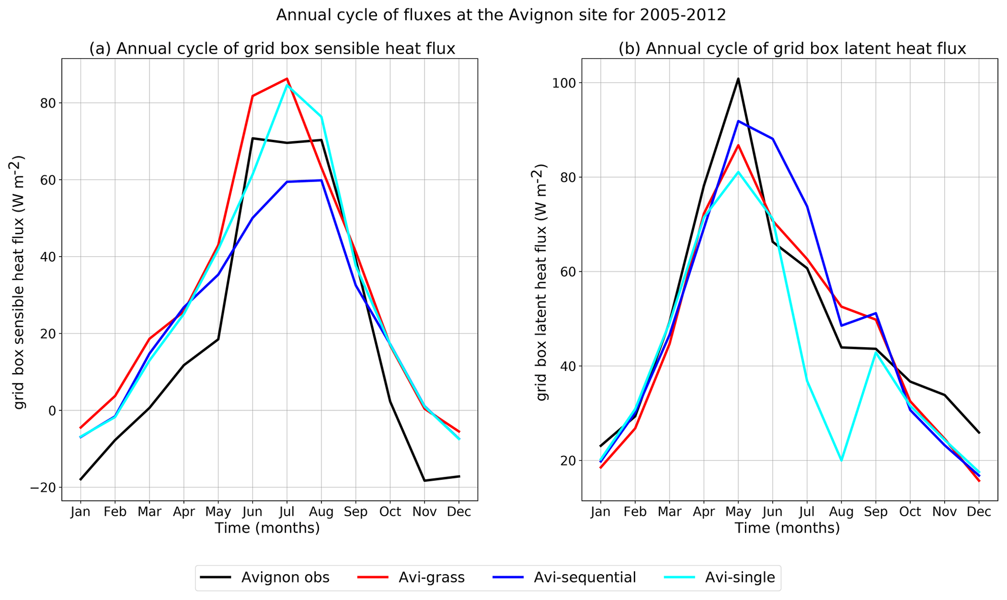
Figure A2 Annual cycle of H (a) and LE (b) compared with observations (black line) at the Avignon site between 2005 and 2013. Annual cycles for the simulations are also shown: Avi-grass (red line), Avi-sequential (blue line) and Avi-single (cyan line).

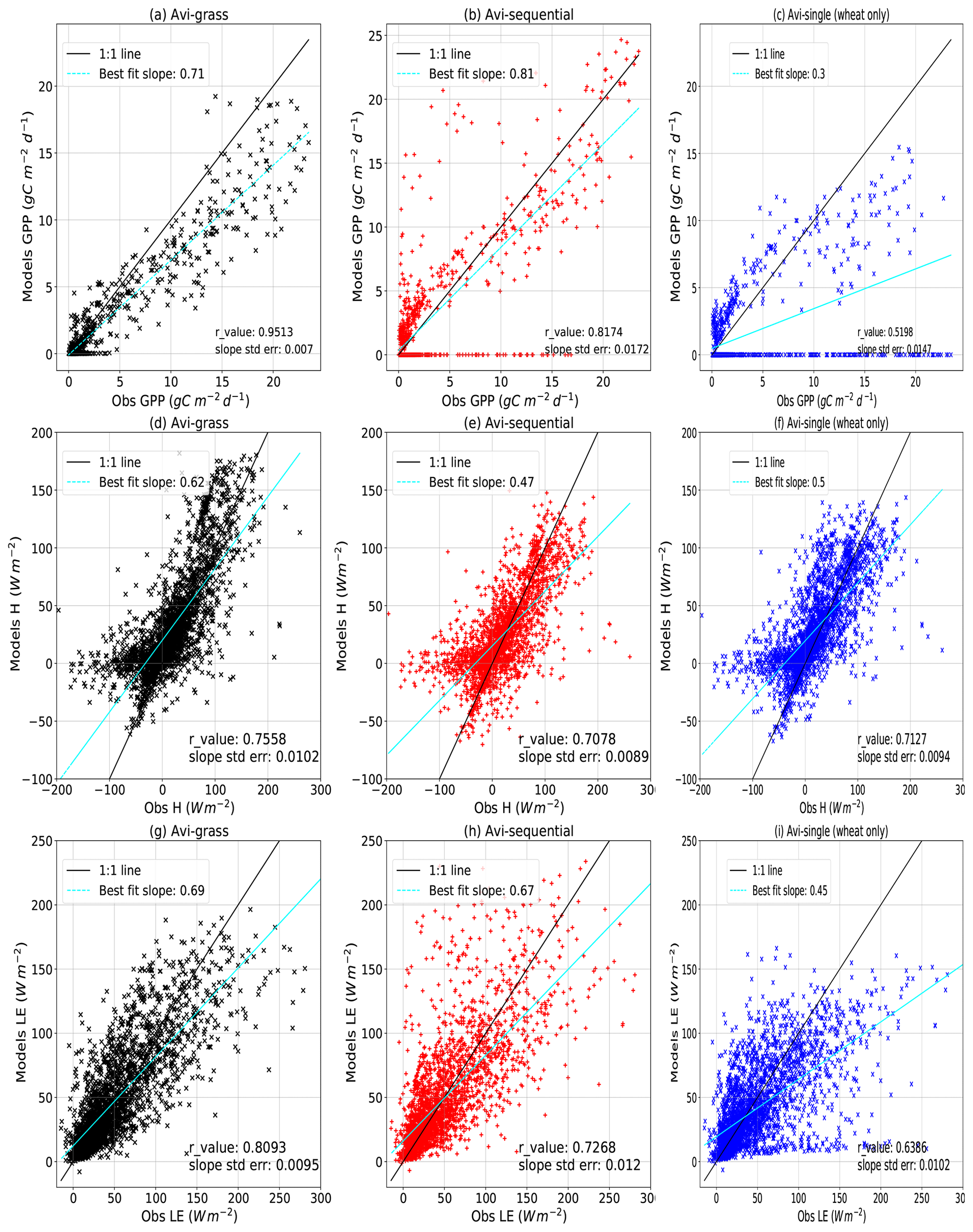
Figure A3 Comparison of observations and model fluxes at the Avignon site: GPP between 2005 and 2008 for Avi-grass (a), Avi-sequential (b) and Avi-single (c). H between 2005 and 2013 for Avi-grass (d) and Avi-sequential (e), Avi-single (f). LE between 2005 and 2013 for Avi-grass (g), Avi-sequential (h) and Avi-single (i).

Appendix B: India single-grid-box comparison

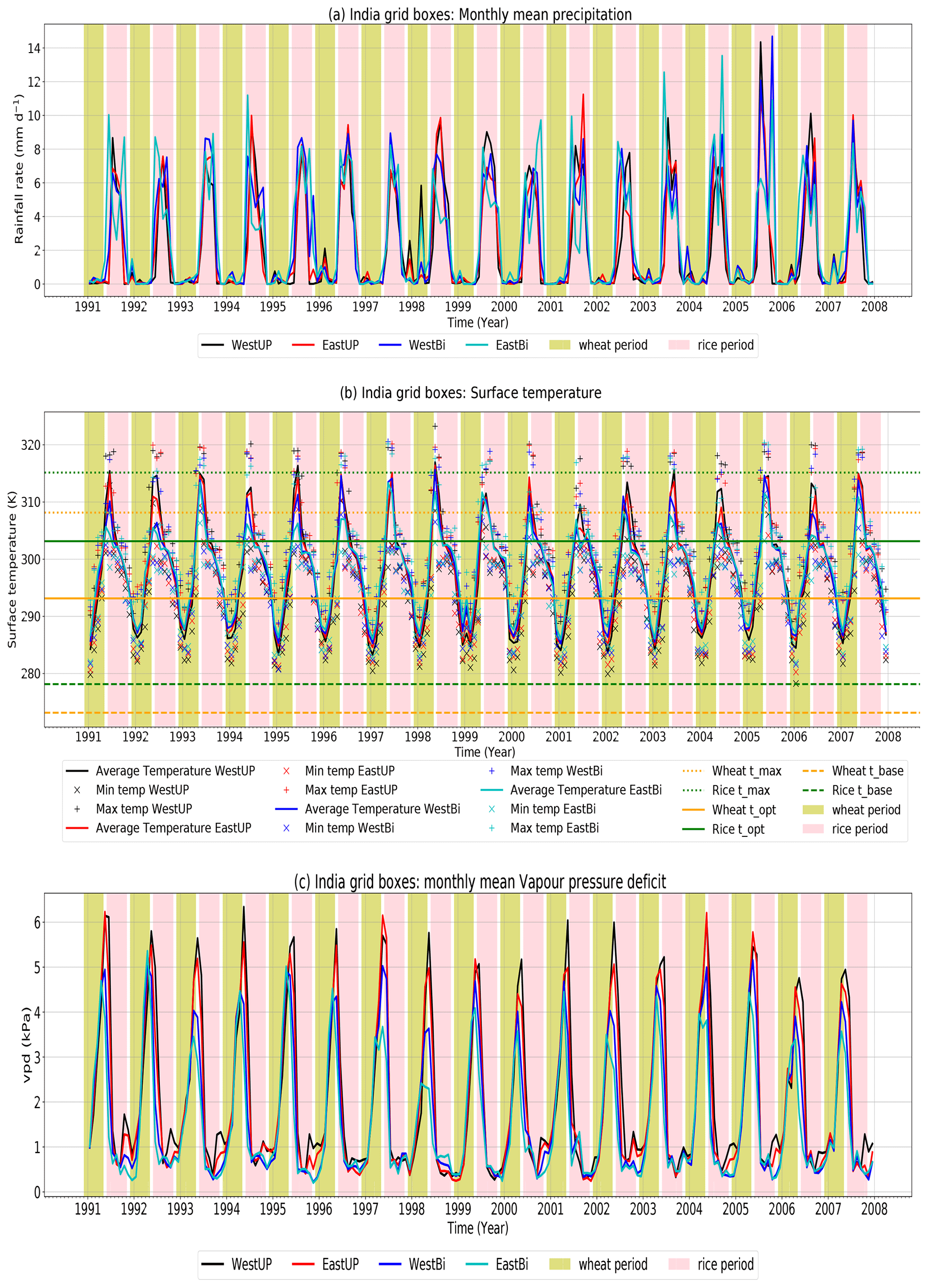
Figure B1 Time series of monthly precipitation (a), temperature (b) and vapour pressure deficit (c) at each of the India locations shown by the solid lines (WestUP – black, EastUP – red, WestBi – blue and EastBi – cyan). Panel (b) also shows the minimum (“×”) and maximum (“+”) temperatures for each of the locations for each month together with the JULES cardinal temperatures (horizontal lines) for rice (green) and wheat (orange): max temperatures (dotted line), optimum temperatures (solid line) and base temperatures (dashed line).

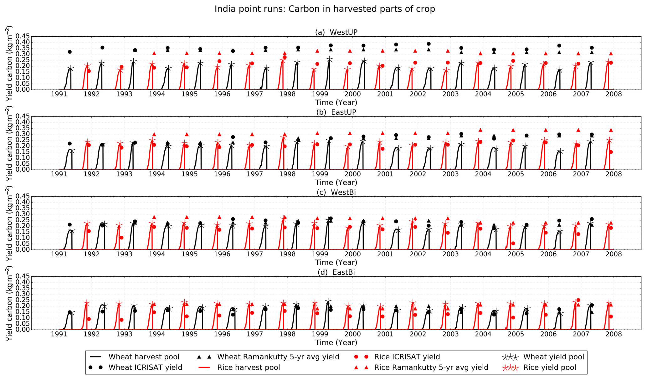
Figure B2 Time series of crop harvest pool (solid lines) with the JULES yield from the sequential-crop run at the time it is output by the model (asterisks) for rice (red) and wheat (black) at each of the India locations shown in Fig. 3. Also shown are two sets of observations: annual yields from ICRISAT (2015) shown by the filled circles and 5-year averages from Ray et al. (2012a) shown by the filled triangles (following the same colours with rice shown in red and wheat in black).

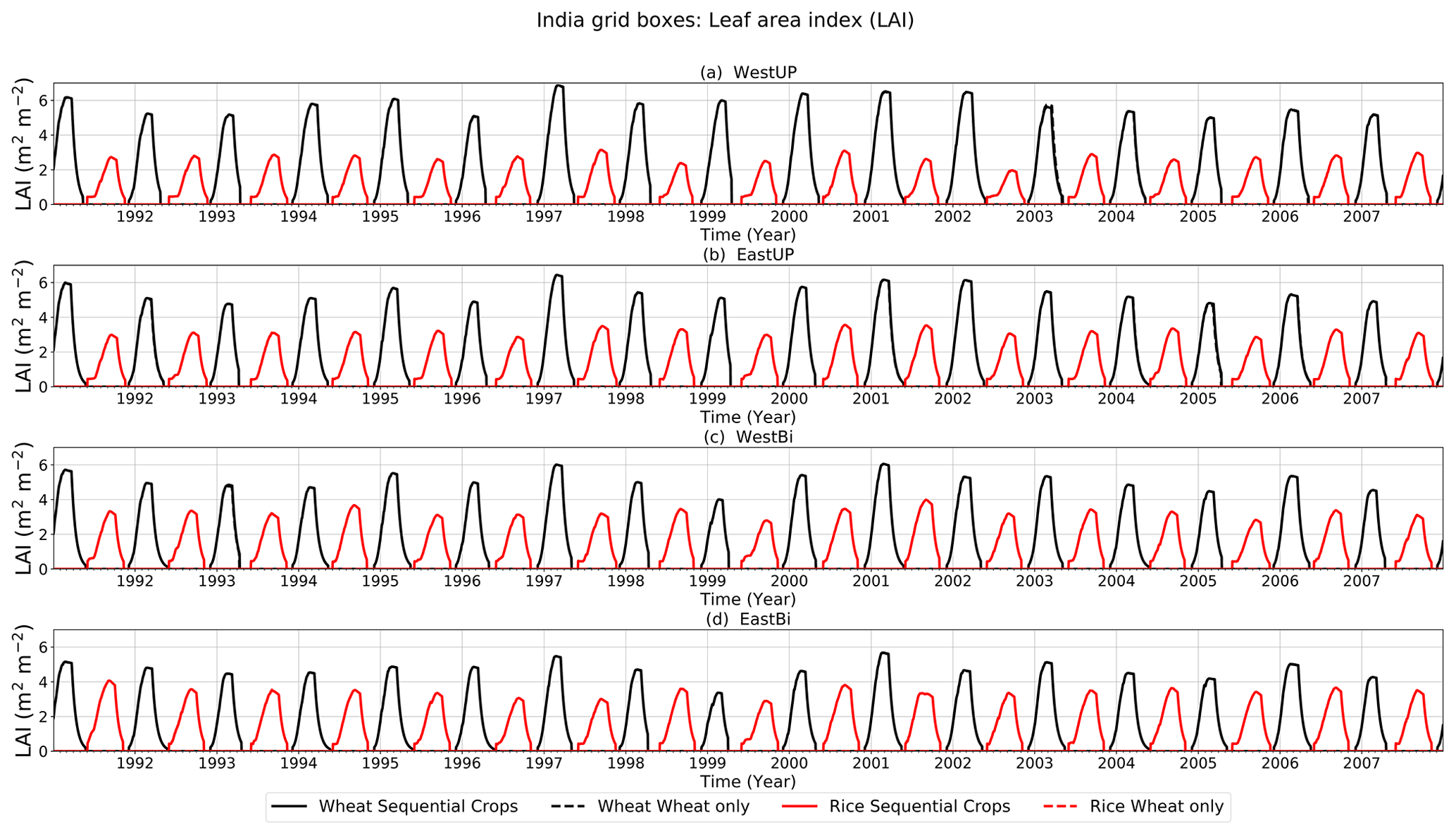
Figure B3 Time series of the LAI of rice (red) and wheat (black) at each of the India locations shown in Fig. 3. India-sequential is shown by solid lines and India-single is shown by dashed lines although they are indistinguishable from each other.

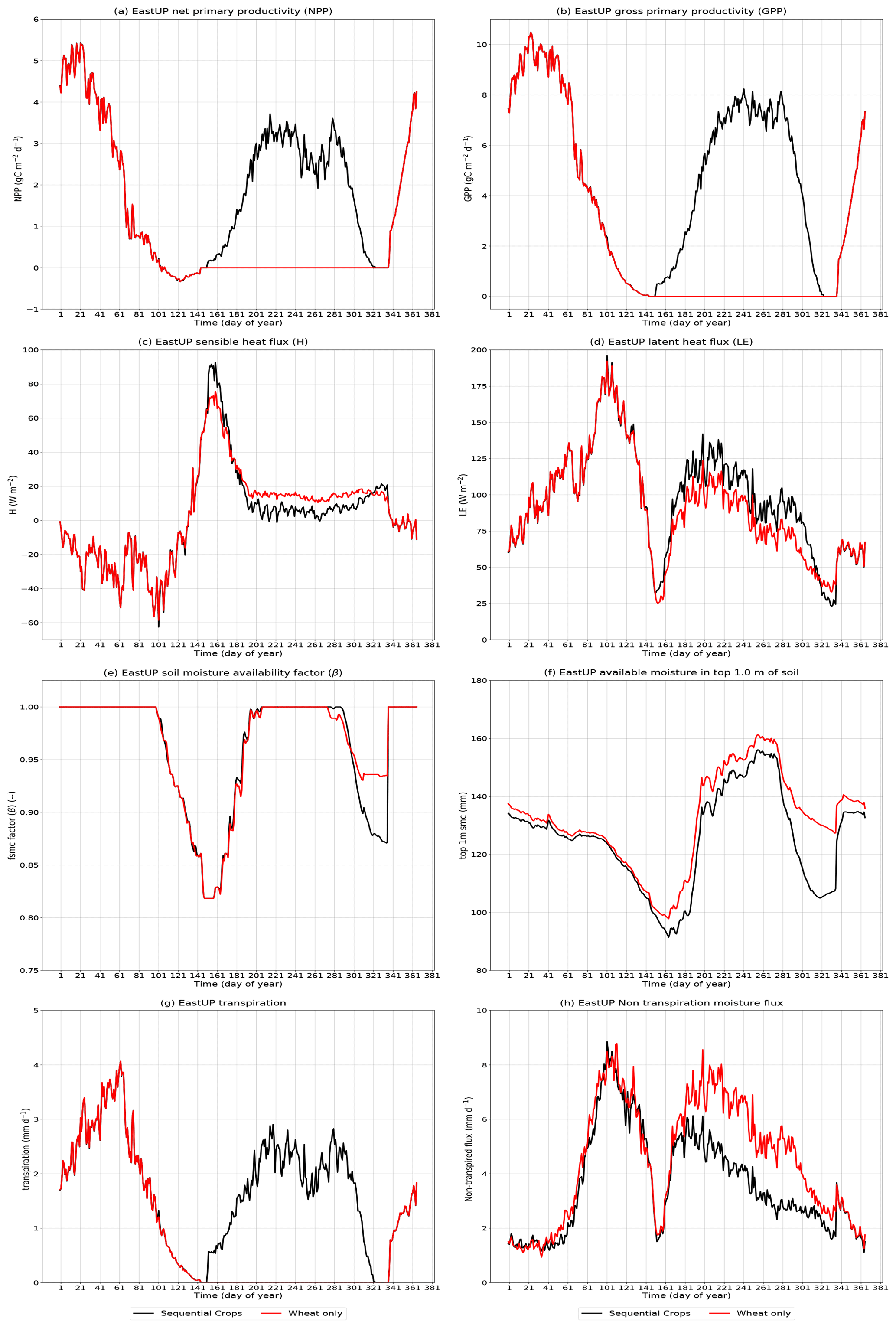
Figure B4 Annual climatology of fluxes (in day of year) for EastUP for India-sequential (black) and India-single (red): carbon fluxes: NPP (a) and GPP (b). Heat fluxes: sensible heat H (c) and latent heat LE (d). Soil moisture variables: β (e) and soil moisture availability in the top 1 m of soil (f). Moisture fluxes: evapotranspiration (g) and non-evapotranspiration moisture fluxes (h).

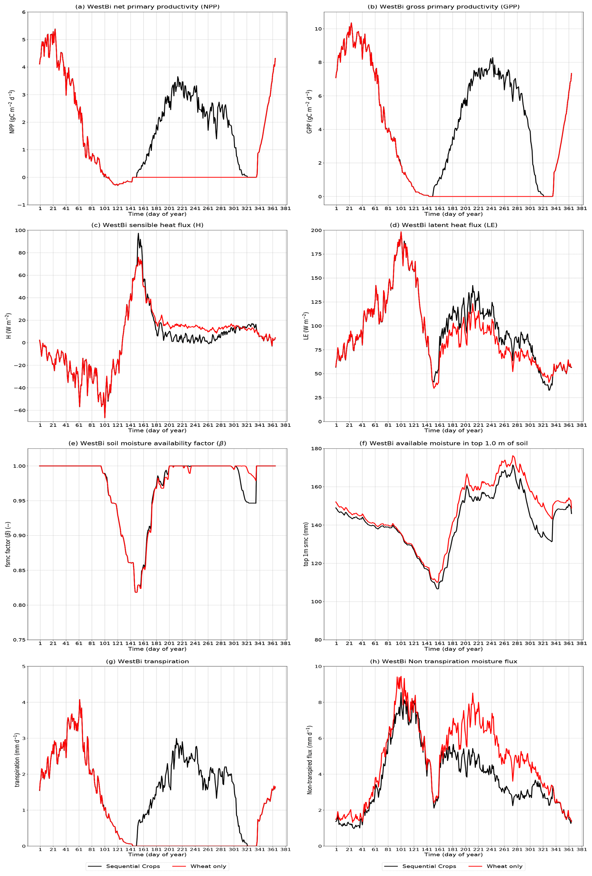
Figure B5 Annual climatology of fluxes (in day of year) for WestBi for India-sequential (black) and India-single (red): carbon fluxes: NPP (a) and GPP (b). Heat fluxes: sensible heat H (c) and latent heat LE (d). Soil moisture variables: β (e) and soil moisture availability in the top 1 m of soil (f). Moisture fluxes: evapotranspiration (g) and non-evapotranspiration moisture fluxes (h).

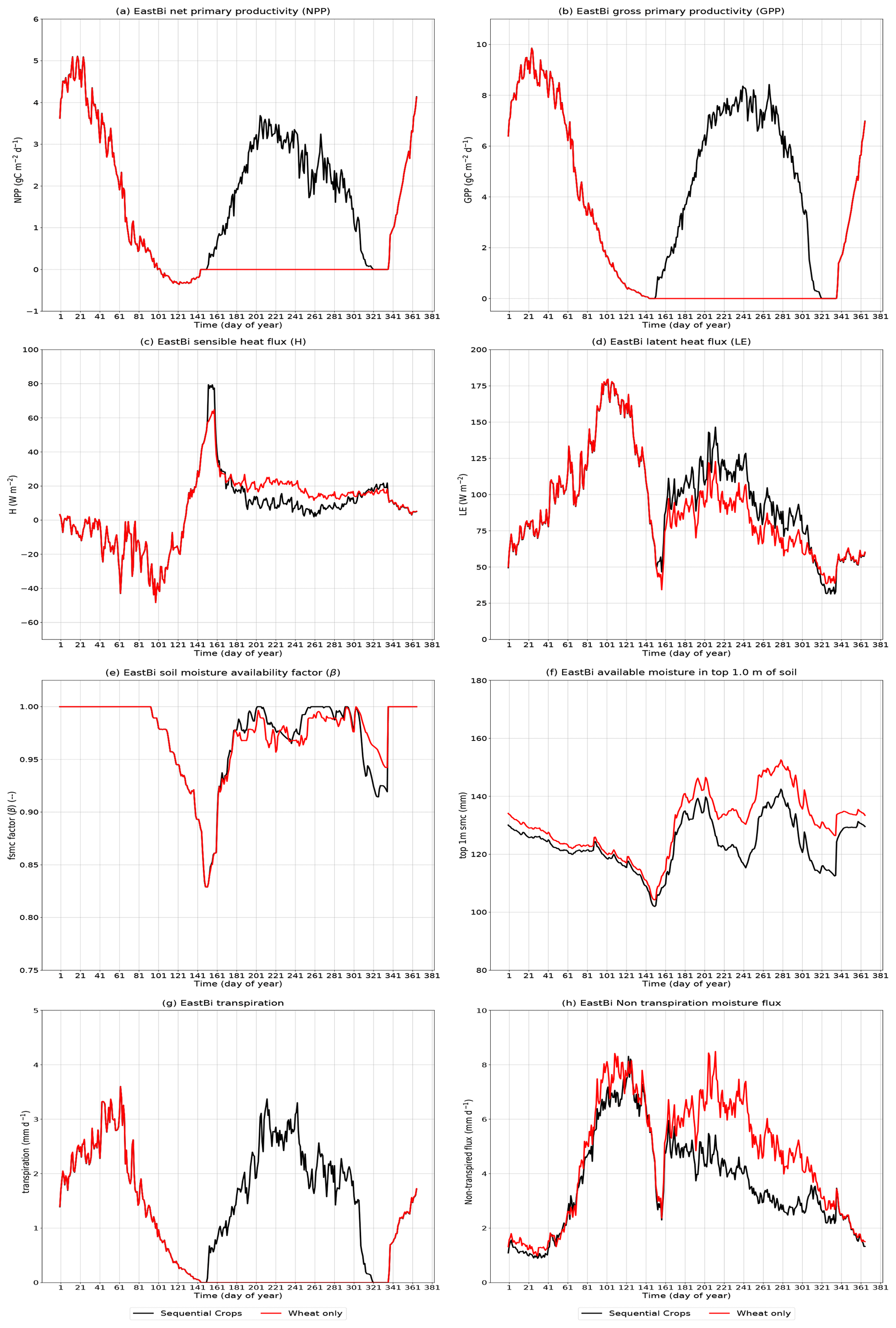
Figure B6 Annual climatology of fluxes (in day of year) for EastBi for India-sequential (black) and India-single (red): carbon fluxes: NPP (a) and GPP (b). Heat fluxes: sensible heat H (c) and latent heat LE (d). Soil moisture variables: β (e) and soil moisture availability in the top 1 m of soil (f). Moisture fluxes: evapotranspiration (g) and non-evapotranspiration moisture fluxes (h).

Figure B7 Time series of each crop carbon pool: leaf (solid lines), root (dashed), stem (dotted) and harvest (dash–dot) with the JULES yield at the time it is output by the model (asterisks) for rice (red) and wheat (black) at each of the India locations shown in Fig. 3 for a subset of years of the simulation between 1998 and 2001.

Appendix C: India regional simulation

.

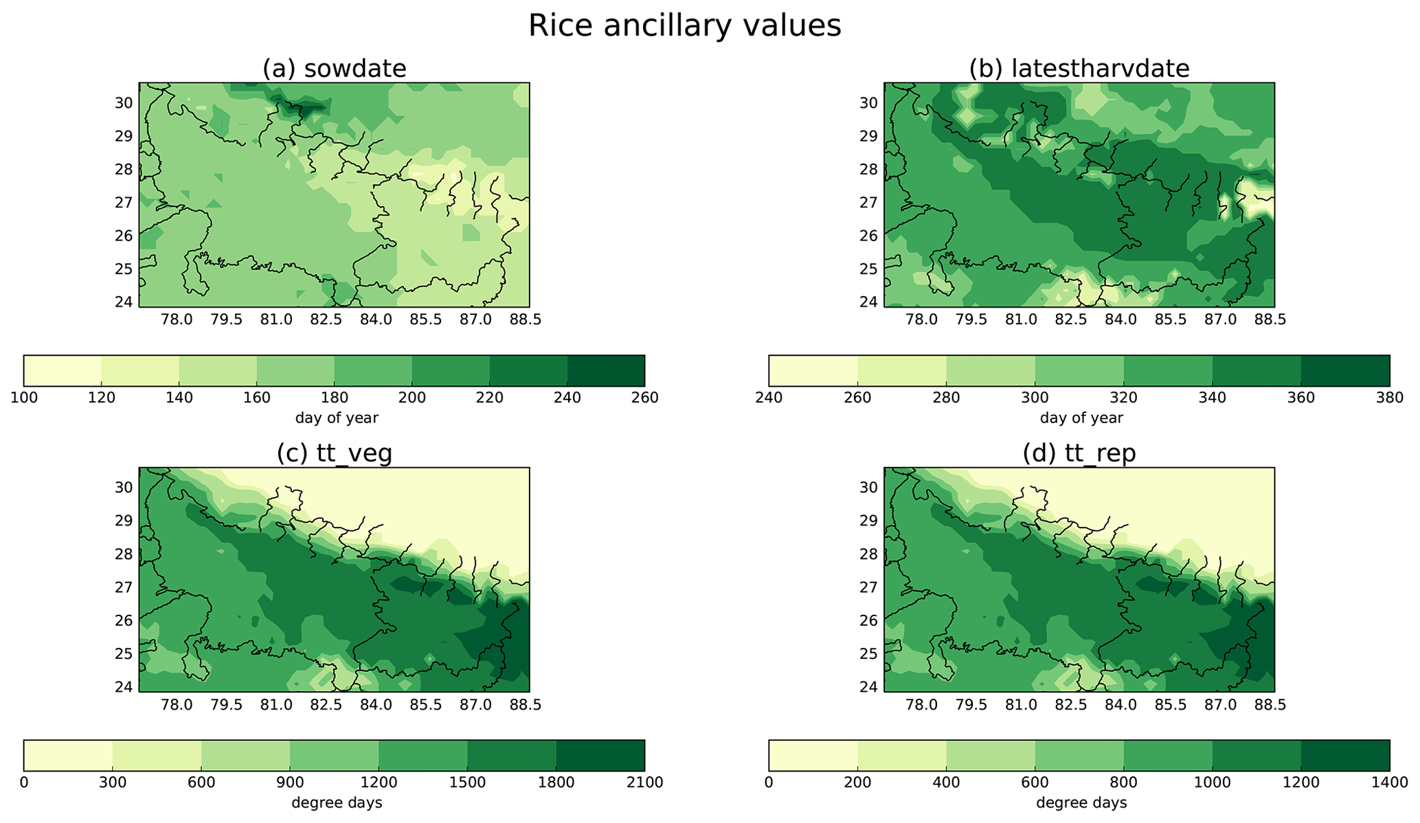
Figure C1 The values used in the regional JULES ancillary for rice. Sowing date (a) and latest possible harvest date (b), both in units of day of year. Thermal time for the vegetative stage (c) and thermal time for the reproductive stage (d), both in units of degree days

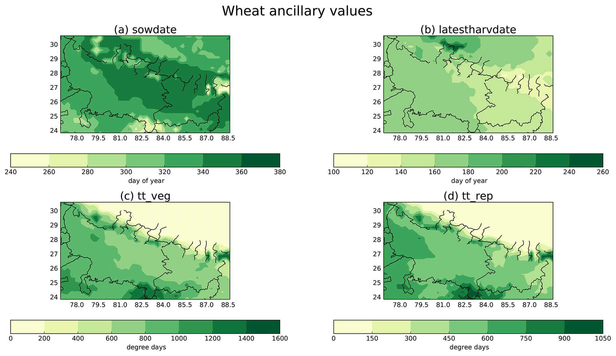
Figure C2 The values used in the regional JULES ancillary for wheat. Sowing date (a) and latest possible harvest date (b), both in units of day of year. Thermal time for the vegetative stage (c) and thermal time for the reproductive stage (d), both in units of degree days.

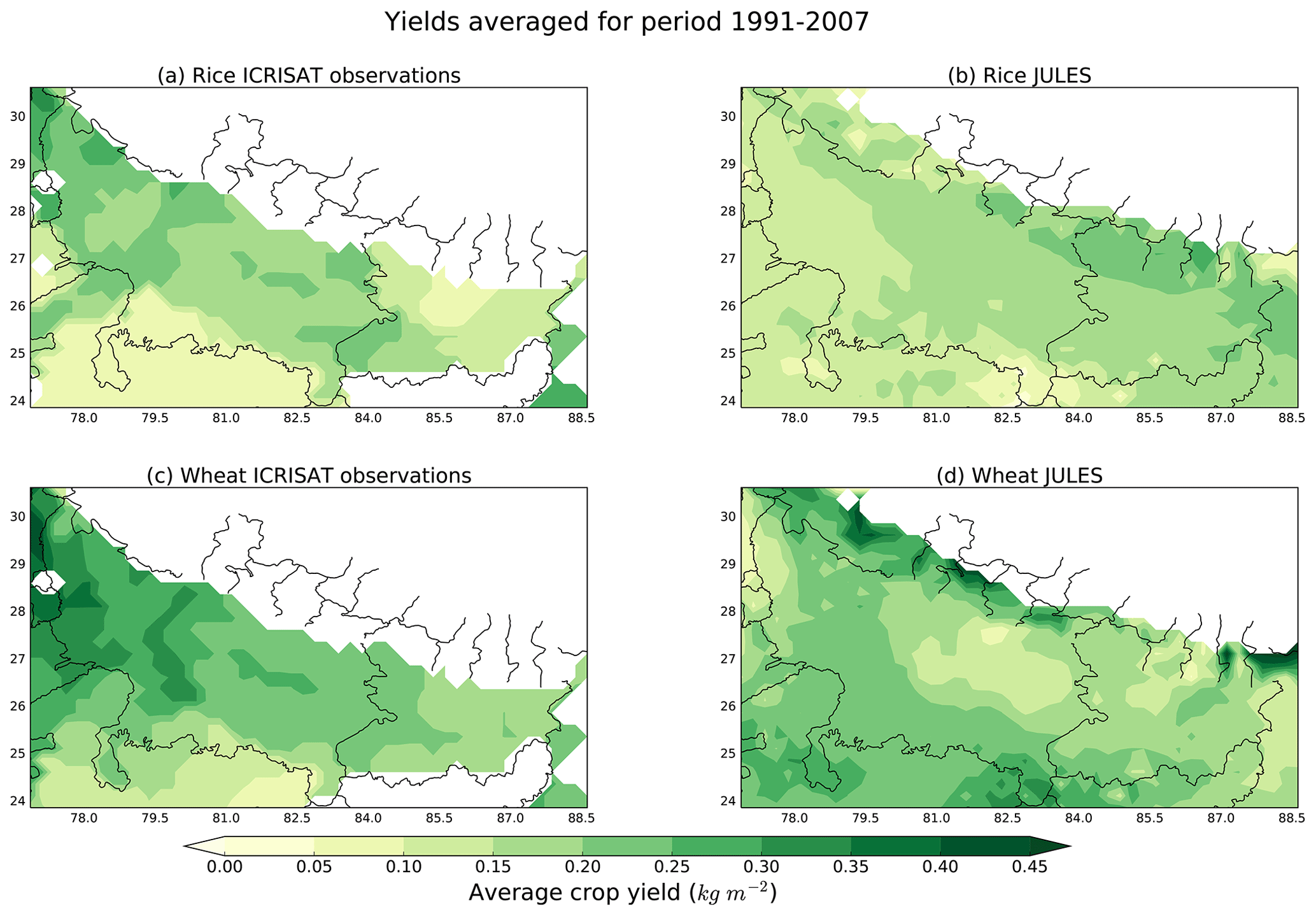
Figure C3 A comparison of observed ICRISAT (2015) rice yields (a) with JULES rice yields (b) and observed ICRISAT (2015) wheat yields (c) with JULES wheat yields (d) for the period 1991–2007 across Uttar Pradesh and Bihar. Note that the simulations assume that rice and wheat are grown everywhere and the crops are not limited by nutrient availability.