Surface representation impacts on turbulent heat fluxes in the Weather Research and Forecasting (WRF) model (v.4.1.3)

The water and energy transfers at the interface between the Earth's surface and the atmosphere should be correctly simulated in numerical weather and climate models. This implies the need for a realistic and accurate representation of land cover (LC), including appropriate parameters for each vegetation type. In some cases, the lack of information and crude representation of the surface lead to errors in the simulation of soil and atmospheric variables. This work investigates the ability of the Weather Research and Forecasting (WRF) model to simulate surface heat fluxes in a heterogeneous area of southern France using several possibilities for the surface representation. In the control experiments, we used the default LC database in WRF, which differed significantly from the actual LC. In addition, sub-grid variability was not taken into account since the model uses, by default, only the surface information from the dominant LC category in each pixel (dominant approach). To improve this surface simplification, we designed three new interconnected numerical experiments with three widely used land surface models (LSMs) in WRF. The first one consisted of using a more realistic and higher-resolution LC dataset over the area of analysis. The second experiment aimed at investigating the effect of using a mosaic approach; 30 m sub-grid surface information was used to calculate the final grid fluxes based on weighted averages from values obtained for each LC category. Finally, in the third experiment, we increased the model stomatal conductance for conifer forests due to the large flux errors associated with this vegetation type in some LSMs. The simulations were evaluated with gridded area-averaged fluxes calculated from five tower measurements obtained during the Boundary-Layer Late Afternoon and Sunset Turbulence (BLLAST) field campaign. The results from the experiments differed depending on the LSM and displayed a high dependency of the simulated fluxes on the specific LC definition within the grid cell, an effect that was enhanced with the dominant approach. The simulation of the fluxes improved using the more realistic LC dataset except for the LSMs that included extreme surface parameters for coniferous forest. The mosaic approach produced fluxes more similar to reality and served to particularly improve the latent heat flux simulation of each grid cell. Therefore, our findings stress the need to include an accurate surface representation in the model, including soil and vegetation sub-grid information with updated surface parameters for some vegetation types, as well as seasonal and man-made changes. This will improve the modelled heat fluxes and ultimately yield more realistic atmospheric processes in the model.

1 Introduction

The Earth's surface is constantly changing at different timescales (Sellers et al., 1995). Natural changes in the land surface (vegetation) occur due to climate variability and seasonality (Weltzin and McPherson, 1997; Crucifix et al., 2005). However, human beings have significantly contributed to non-natural and accelerated changes in land cover (LC), especially during recent decades (Pielke et al., 2011). These changes can be extremely important because they modify the natural cycles of energy (Seneviratne et al., 2010), trace gases (e.g. Muñoz-Rojas et al., 2015; Green et al., 2019), and nutrients (e.g. Holmes et al., 2005), among others, and because they alter ecosystems (Pielke et al., 1998). The consequences of these alterations are difficult to predict due to the non-linearity of the numerous connected processes (Pielke et al., 1999). On the one hand, changes in habitat alter food chains and impact vegetal and animal species (Auffret et al., 2018), but also smaller organisms living within them or in equilibrated soil, such as bacteria and viruses (Jeffery and Van der Putten, 2011; Blackburn et al., 2007; Rulli et al., 2020). On the other hand, radiative and texture properties of the surface are also modified: changes in albedo (Loarie et al., 2011), emissivity, thermal properties of the soil (Luyssaert et al., 2014), and surface roughness (Bonan et al., 2018). This modifies the heat and water exchange processes between the surface and the atmosphere by altering the net radiation at the surface. Indeed, water transfers from the soil to the air (and vice versa) are significantly linked to the vegetation type and soil properties: infiltration, runoff, soil moisture, and evapotranspiration (ET) (Zhang and Schilling, 2006). All these changes in the surface energy balance have direct or indirect feedbacks on the planetary boundary layer (PBL) development (Combe et al., 2015), cloud formation (Vilà-Guerau De Arellano et al., 2012), atmospheric temperatures (Koster et al., 2006; Christidis et al., 2013), and rainfall (Koster et al., 2003). This may impact surface characteristics and vegetation activity again, and in the long term it will restart the whole cycle by changing species (vegetation included), which need to adapt to the modified environmental conditions (Pielke et al., 1998), with the direct or indirect associated impacts on the first triggers: the humans (Meyer and Turner, 1994; Rulli et al., 2020).

Since LC change decisions are typically made by local and regional governments (e.g. Sánchez-Cuervo et al., 2012), it is of utmost importance that these organizations understand the direct and indirect implications of various anthropogenic Earth surface modifications. Hence, it is crucial to quantify the uncertainty associated with land surface representation in weather and climate models, which is the main objective of this paper.

Current weather and climate models rely on parameterizations to represent energy, water, and momentum exchanges between the surface and the atmosphere. This is done by coupling land surface models (LSMs) with the atmospheric component of the predicting system. During the last decades, significant effort has been made to improve LSMs (Cuxart and Boone, 2020). On the one hand, their complexity has been increased with equations that are able to represent the myriad of processes involved in these exchanges (Lawrence et al., 2019). On the other hand, these equations need accurate parameters that describe the properties of the soil and the vegetation (Cuntz et al., 2016). Both types of improvements need observational measurements from experimental sites and field campaigns to learn about surface properties and physical processes, as well as to evaluate models.

In this context, numerous scientific initiatives have been conducted to improve knowledge of the land–atmosphere interaction processes. This has been done through the design of experimental field campaigns: e.g. the Boreal Ecosystem Atmosphere Study (BOREASl; Sellers et al., 1995), the Global Energy and Water Cycle Experiment (GEWEX; Chahine, 1992), and the Lindenberg Inhomogeneous Terrain – Fluxes between Atmosphere and Surface: a Long-term Study (LITFASS; Beyrich et al., 2002), among many others. Other initiatives were focused on the intercomparison of LSMs: e.g. the Project for Intercomparison of Land-surface Parameterization Schemes (PILPS; Henderson-Sellers et al., 1996) and the Global Land–Atmosphere Coupling Experiment (GLACE; Koster et al., 2006). Recently, the CloudRoots field experiment (Vilà-Guerau de Arellano et al., 2020) offered an integrated multi-scale approach from leaf to landscape measurements complemented with models.

Some specific works have also focused on the effect of LC through the investigation of the impacts of improving the accuracy and resolution of LC databases used in the models (e.g. Pineda et al., 2004; Cheng et al., 2013; Santos-Alamillos et al., 2015; Schicker et al., 2016; Jiménez-Esteve et al., 2018). Others have focused on modelling the changes that might occur under the assumption of possible future changes to the surface (e.g. Li et al., 2018; De Meij et al., 2019). These studies stated the importance of having an accurate surface representation in the models to obtain improved simulations of different variables.

In this sense, the present work was firstly motivated by the inaccurate representation of the LC provided by the default LC dataset (International Geosphere–Biosphere Programme from the Moderate Resolution Imaging Spectroradiometer, IGBP-MODIS) in the Weather Research and Forecasting (WRF) model over the area of analysis (southern France), which differed significantly from the LC observed in the area. We hypothesized that this would lead to errors in the simulated surface energy fluxes (specifically, sensible and latent heat fluxes). Also, the default configuration in WRF only uses the information from the tabulated surface parameters of the LC category with a higher percentage of coverage within each grid cell (dominant approach). This may be appropriate for areas with sufficiently large homogeneous surfaces, but not for the area of study, where the LC has significant heterogeneous patches that might impact the surface fluxes. This influence of the surface heterogeneous patches on the lower troposphere is known as static heterogeneity (e.g. Patton et al., 2005; van Heerwaarden and Guerau de Arellano, 2008) and also has impacts on the PBL processes (e.g. Margairaz et al., 2020a, b), creating new (dynamical) inhomogeneities such as clouds or modified turbulence. This will also impact the surface in an interaction known as dynamical heterogeneity (e.g. Lohou and Patton, 2014; Horn et al., 2015).

This study is focused on the static heterogeneity impacts on surface fluxes through the quantification of the changes associated with several improvements made to the representation of the surface in the WRF model, which is the main objective of this work. In order to strengthen the analysis, three widely used LSMs available in WRF were used: (1) Noah (Chen and Dudhia, 2001), (2) Noah-MP (Multi-Physics) (Niu et al., 2011), and (3) RUC (Rapid Update Cycle) (Smirnova et al., 2016). The different experiments were designed as follows. First, we improved the LC in the area evaluated using the more realistic and higher-resolution LC dataset from the Centre d'Etudes Spatiales de la Biosphère research laboratory (CESBIO; Inglada et al., 2017). The results showed a high dependence of the flux on the specific LC categories, which motivated a second experiment including the sub-grid information on the surface, the so-called mosaic approach (e.g. Li et al., 2013). Finally, an additional experiment was carried out due to the extreme biases found in the first two experiments over pixels mostly covered by conifer trees in Noah-MP, with the aim of diminishing the biases by modifying some parameters associated with the transpiration processes of this LC category.

For the evaluation of the simulations, we took advantage of the large number of instruments deployed during the Boundary-Layer Late Afternoon and Sunset Turbulence (BLLAST) field campaign, carried out in 2011 in southern France (Lothon et al., 2014). The spatial density of eddy-covariance (EC) towers over different vegetation types facilitated the calculation of gridded area-averaged fluxes (AAFs), as done in a similar way for the LITFASS experiment (Beyrich et al., 2006), for which good agreement with the fluxes measured from scintillometry was obtained. In the present work, the AAFs were used to evaluate the results from the WRF model coupled with the three LSMs under the different conditions set in the experiments, and to analyse the results based on the different LC types.

The article is organized as follows: Sect. 2 provides information on the measurements taken during the BLLAST field campaign and explains how the area-averaged fluxes were calculated. Detailed information about the model configuration and the different experiments is also included in this section. In Sect. 3, we quantify the results from the different modelling experiments, including scientific discussion about them. Finally, a short summary and the main conclusions are provided in Sect. 4.

2 Evaluation data, WRF model, and experimental design

2.1 Observational data for model evaluation

The surface turbulent heat fluxes simulated by the WRF model were evaluated during a period of the BLLAST field campaign (Lothon et al., 2014). This campaign took place from 14 June to 8 July 2011 on the Plateau of Lannemezan (southern France). Its main objective was to better understand the turbulence decay observed during the afternoon transition, and the extensive instrumentation deployment included several surface-energy-balance towers installed over different surfaces, which were representative of the vegetation within the explored area: prairies, forests, wheat, corn, and moor. The analysed period was from 09:00 UTC to 15:00 UTC on 19 June 2011, corresponding to part of IOP 2 during the campaign (IOP: intensive observation period). This IOP was characterized by fair weather, no clouds, and a typical development of the boundary layer up to 800–1000 m above ground level (a.g.l). The IOP is representative of the general conditions of the rest of the IOPs of the campaign (the general meteorological conditions of the campaign can be found in Lothon et al., 2014).

2.1.1 Observed fluxes over different vegetation types

SH and Le were calculated uniformly using the eddy-covariance (EC) method with the specifications indicated in De Coster et al. (2011) over five different LC types: grass, wheat, corn, moor, and forest (conifers). The height of the instruments above ground level (a.g.l.) was set according to the vegetation height, which implied a homogeneous footprint for the five towers: 2 m for the moor, grass, and wheat sites, 4 m for the corn site, and 31 m for the forest site (approx. 6 m above the trees). These measurements showed that the SH was more sensitive to LC type (Fig. 1a and c) than Le (Fig. 1b and d). This was probably linked to the different surface properties of the vegetation types (albedo, thermal inertia, emissivity), with more influence on the surface temperatures. The highest SH was measured over the forest site, followed by the wheat site, with peaks of around 400 and 270 W m⁻², respectively. The measurements over the grass, moor, and corn sites showed lower values, with a maximum SH of around 150 W m⁻² during the central hours of the day. However, Le exhibited values that were similar for all the vegetation types, with midday maxima around 300 W m⁻². Nevertheless, the lowest Le was measured over the wheat field (this crop started to dry during the experiment), while the largest values were observed at the grass, forest, and moor sites. Some differences were observed in the diurnal evolution of Le: the morning Le rise over the corn and wheat was delayed with respect to the measurements over other LCs, maybe linked to a delay in the transpiration processes associated with these crops (a full investigation of the reasons for it is out of the scope of this study). In any case, it should be highlighted that these flux values were representative of those of the different IOPs of the BLLAST field campaign (Lothon et al., 2014; Couvreux et al., 2016), with no water limitation due to the regular rain events observed in the area during the weeks before, which are typical conditions for these dates in the area.

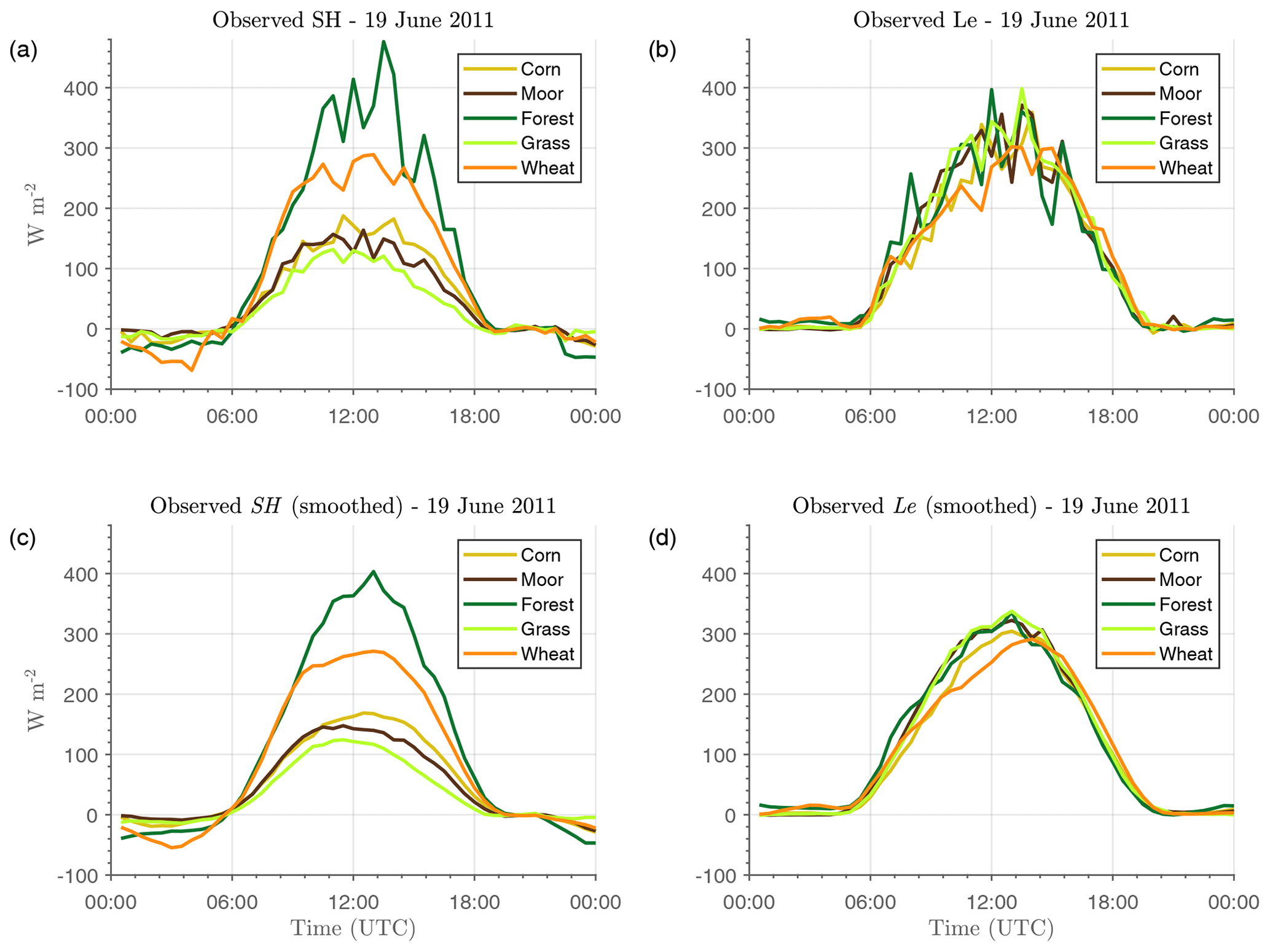
Figure 1 (a) Observed sensible heat flux (SH) on 19 June 2011 during the BLLAST campaign over different vegetation types. (b) The same for the latent heat flux (Le). (c, d) Same as in (a) and (b), but with the time series smoothed for a better visualization of the main differences between vegetation types. The flux values were calculated using the eddy-covariance technique with averaging windows of 30 min.

2.1.2 Area-averaged flux (AAF) calculation

The EC measurements from towers were used for the calculation of AAF with a resolution of 1 km in a region of 19×19 km around the central site of the field campaign: 43^∘07^′27.15^′′ N, 0^∘21^′45.33^′′ E; 600 m above sea level (a.s.l.). This approach can be considered a mosaic observational method for flux computation. It was based on the multiplication of the values of the fluxes measured over each vegetation type by their respective vegetation cover fraction within each 1×1 km pixel (see Fig. 2a and b). Finally, the contribution from each vegetation type was summed to provide the final values in each grid cell (area-averaged fluxes). High-resolution and realistic LC data were needed to construct the AAF, which were obtained from the 30 m LC database prepared by CESBIO based on Landsat-5 data (Inglada et al., 2017) (Fig. 2b). Hence, the main assumption of the AAF calculation was to consider the same SH and Le for sites with the same LC type at different locations, also implying the following simplifications (a further discussion is included after the list).

1. There were no flux differences depending on the soil type.

2. There was no difference in activity for the same vegetation type in the area.

3. There was no horizontal variability of the soil moisture (SM).

4. The radiation and the wind forcing was the same for all the pixels, without altitude influences.

5. All the forests were considered coniferous (evergreen needleleaf forest – ENF).

6. Fluxes over urban and bare soil surfaces were estimated using a simple model.

(1) Two soil types were the dominant ones in the evaluation area based on the 1×1 km pixels from the soil database of WRF (United States Department of Agriculture, USDA): clay loam (81 % of the area) and loam (19 % of the area). Since the dominant soil type in the pixels wherein the measurements were taken was clay loam, pixels with loam were not included in the evaluation of the model. Therefore, the limitation based on the soil type was ultimately not a problem. This area is shown in Fig. 2d with a black rectangle.

(2) The area analysed is relatively small to expect significant differences between the natural vegetation belonging to the same category. Although the limitation based on the possible different vegetation state can be more important in crop areas, seeding dates are normally coincident between fields in the area.

(3) Regarding the effect of possible SM differences within the area, two aspects should be noted. On the one hand, the potential SM horizontal variability due to possible inhomogeneous precedent rainfall over the area was not taken into account. However, the SM input in the model is provided with a coarse resolution of 1^∘ and does not show any small-scale details. This is a well-known limitation of mesoscale models which is sometimes addressed through the assimilation of SM data from satellites or with previous long simulations that serve to spin up the surface in order to obtain the appropriate SM initial values (De Rosnay et al., 2013; Angevine et al., 2014; Santanello et al., 2016). In our case, this limitation of mesoscale modelling is an advantage because it allows us to perform a fairer model–observation comparison since this limitation also exists in the AAF. The impact of applying a spin-up period to the model is investigated later.

On the other hand, some of the SM horizontal variability is caused by the different properties of the vegetation patches, affecting runoff, infiltration, evapotranspiration, and finally the SM content associated with each vegetation type. This LC effect on SM may be implicitly included in the fluxes that were measured over each individual vegetation type. In any case, we investigated the effect of including the SM horizontal heterogeneity with a higher resolution in the model initialization (not shown). This was done by using high-resolution SM satellite data from the Disaggregation based on Physical And Theoretical scale Change (DISPATCH) (Merlin et al., 2013; Molero et al., 2016) product at 1 km of resolution, but conserving the original range of SM variability within the area evaluated. The effect of including this SM spatial heterogeneity was minimal in the flux simulations (in part due to the conservation of the range of SM values).

(4) The limitation due to the radiation and wind forcing, which were assumed to be equal in all the pixels, is expected to have a small impact due to the fair weather, with no clouds, and light wind conditions on 19 June (Lothon et al., 2014). However, some differences could exist between some pixels situated at different altitudes over the area (most of the pixels were in the range of altitude between 400 and 650 m a.s.l., with minimum and maximum altitude of 282 and 696 m a.s.l. in the whole evaluated area).

(5) The limitation of considering all forests to be coniferous was due to the fact that the campaign only included measurements over this type of tree, and not over broadleaf deciduous forests (the other forest category in the area). Therefore, the measurements taken over conifers were extrapolated to areas covered by deciduous for the calculation of the AAF. This limitation was addressed by converting all the forest in the WRF model to conifer, which allowed a fairer model–observation comparison at the expense of losing the analysis over one LC category (deciduous forest).

(6) For the urban surfaces, SH and Le were calculated following a simple Penman–Monteith type model (De Bruin and Holtslag, 1982) shown in Eqs. (1) and (2), respectively:

$$\begin{array}{}\text{(1)}& {\displaystyle }\text{SH}=\mathit{\beta }\cdot {\displaystyle \frac{R_{\mathrm{n}}-G}{\mathrm{1}+\mathit{\beta }}},\text{(2)}& {\displaystyle }\text{Le}={\displaystyle \frac{R_{\mathrm{n}}-G}{\mathrm{1}+\mathit{\beta }}},\end{array}$$

where R_n (Eq. 3) is the net radiation, defined as

$$\begin{array}{}\text{(3)}& R_{\mathrm{n}}=(\mathrm{1}-\mathit{\alpha })\cdot \text{SW}\downarrow +\text{LW}\downarrow -\mathit{ϵ}\mathit{\sigma }{T}_{\mathrm{s}}^{\mathrm{4}},\end{array}$$

and G (Eq. 4) is the ground heat flux, considered a fixed fraction of R_n:

$$\begin{array}{}\text{(4)}& G=G_{\mathrm{frac}}\cdot R_{\mathrm{n}}.\end{array}$$

In these equations, SW↓ and LW↓ are the measured downward shortwave and longwave radiative fluxes, respectively. The albedo (α), emissivity (ϵ), the fraction of energy used for ground heat flux (G_frac), and the Bowen ratios (β) were considered constant, with values of 0.15, 0.92, 0.3 (stable) $/$ 0.5(unstable), and 5, respectively, obtained from Lemonsu et al. (2004) and Grimmond and Oke (1999) for urban surfaces. These simplifications could have led to some overestimation of the urban effect on the total fluxes, since the urban surfaces in the area were surrounded by gardens, prairies, and trees (so-called urban diffuse in the CESBIO LC dataset). However, the 30 m resolution LC dataset should be appropriate to deal with the urban and vegetation patches.

Despite the high-quality data and the efforts made to reduce uncertainties in the AAF, the evaluation of models with surface observations is a necessary task which is not straightforward. The observational measurements are almost always linked to uncertainties that can add limitations to the evaluation process (Bou-Zeid et al., 2020). In our case, the measurements were taken at heights that implied homogeneous footprints, but even in this case, other uncertainties are always present (Mauder et al., 2020), especially in the case of the measurements taken over vegetation with tall canopies, where heat storage can have an important role in the surface energy balance.

2.1.3 Performance scores

Three performance scores were used to evaluate the modelled fluxes using the AAF as a benchmark. The first one is $\stackrel{\mathrm{‾}}{\text{Bias}}$ (Eq. 5), which is subsequently referred to as the bias:

$$\begin{array}{}\text{(5)}& \stackrel{\mathrm{‾}}{\text{Bias}}={\displaystyle \frac{{\displaystyle }\sum _{i=\mathrm{1}}^N[{\text{Flux}}_{\mathrm{sim}\left(i\right)}-{\text{Flux}}_{\mathrm{obs}\left(i\right)}]}{N}},\end{array}$$

where Flux_sim(i) is the simulated SH or Le for each grid cell and each analysed hour, with N being the total number of data used, and Flux_obs(i) is the respective value computed from the AAF (observations). The average was performed for all the analysed hours (from 09:00 to 15:00 UTC) and for all the grid cells covered by a certain land cover category within the analysed area (note how in Table 3 these values are averaged for the whole area without land cover distinction). Hence, although the bias provides an indication of the systematic overestimation or underestimation of the modelled flux, the averaging can lead to undesired conclusions, since positive and negative values can compensate in some cases (especially if contrasting LC categories are merged).

We also include the root mean square error (RMSE), which is the root mean of the squared differences between the model and observed fluxes at each analysed hour and for all the grid cells with a certain land cover category:

$$\begin{array}{}\text{(6)}& \text{RMSE}=\sqrt{{\displaystyle \frac{{\displaystyle }\sum _{i=\mathrm{1}}^N[{\text{Flux}}_{\mathrm{sim}\left(i\right)}-{\text{Flux}}_{\mathrm{obs}\left(i\right)}{]}^{\mathrm{2}}}{N}}}.\end{array}$$

Finally, the standard deviation of the error (Eq. 7) is also included, which provides an indication of the model random error; i.e. values close to zero will indicate that the model error tends to be systematic, while large values indicate that the error is variable and randomly distributed:

$$\begin{array}{}\text{(7)}& \text{SD}=\sqrt{{\displaystyle \frac{\mathrm{1}}{N-\mathrm{1}}}{\displaystyle }\sum _{i=\mathrm{1}}^N\left|\right[{\text{Flux}}_{\mathrm{sim}\left(i\right)}-{\text{Flux}}_{\mathrm{obs}\left(i\right)}]-\stackrel{\mathrm{‾}}{\text{Bias}}{|}^{\mathrm{2}}}.\end{array}$$

2.2 WRF model

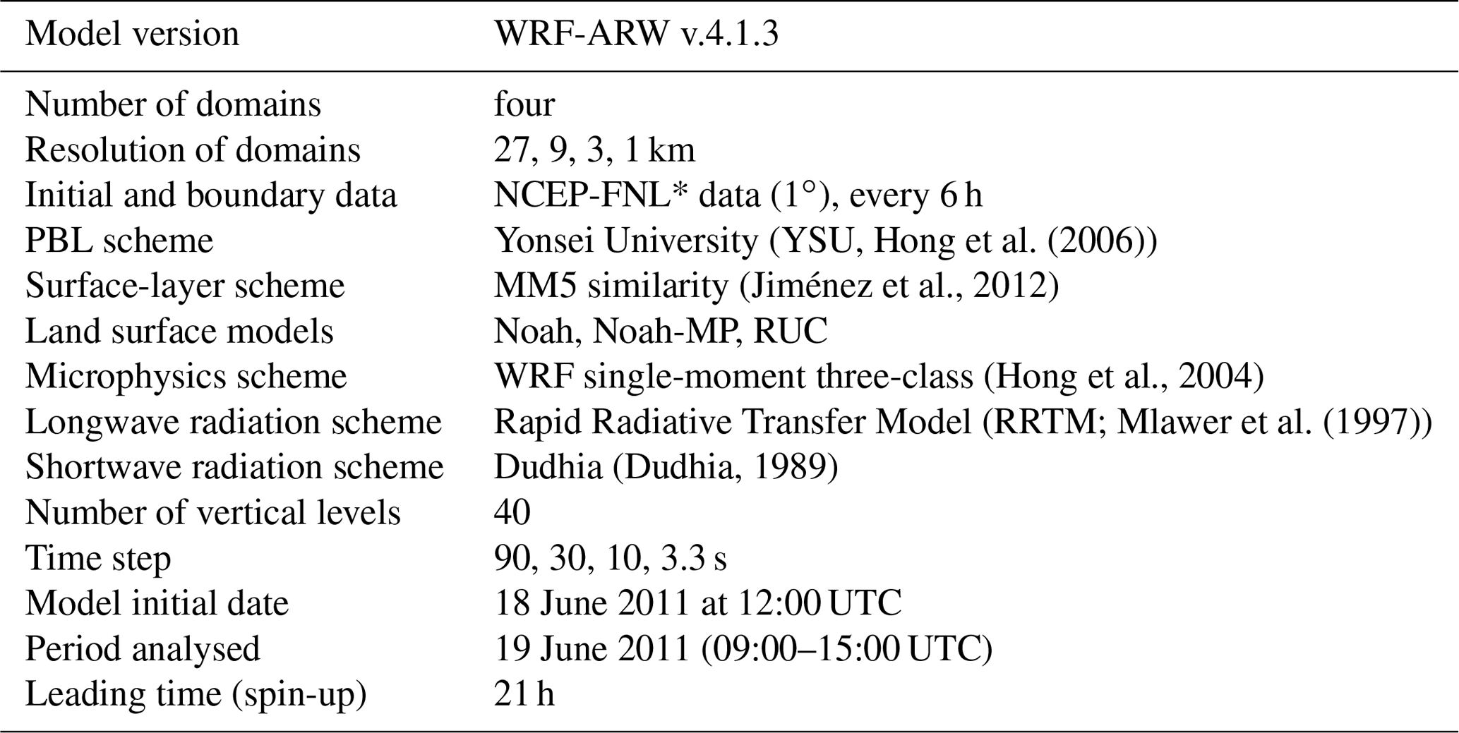
The WRF-ARW (Weather Research and Forecasting–Advanced Research WRF) v.4.1.3 (Skamarock et al., 2019) was used to run the different numerical experiments. The model ran for 60 h (from 12:00 UTC on 18 June 2011 to 00:00 UTC on 21 June), but only the central hours of 19 June were evaluated. The first 21 h of the simulation were used as spin-up, and the diurnal cycle of 20 June was not analysed due to the presence of clouds in the area, which made it more difficult to carry out the strategy designed for the main objective (Pedruzo-Bagazgoitia et al., 2017). The simulations were configured with four nested domains of 27, 9, 3, and 1 km resolution.

The inner domain covered an area of 120×120 km², but only an area of 19×19 km² around the central point was evaluated, which had the same grid as the AAF used for the evaluation; i.e. the centre of the central pixel was located at the same location as the centre of the AAF used for the evaluation. More details about the WRF technical configuration common to all experiments are included in Table 1.

Hong et al. (2006)(Jiménez et al., 2012)(Hong et al., 2004)Mlawer et al. (1997)(Dudhia, 1989)

Table 1 Details about the WRF model configuration common to all simulations. *National Centers for Environmental Protection (NCEP) FNL (final) Operational Model Global Tropospheric Analyses, continuing from July 1999 (NCEP, 2000).

2.2.1 WRF land surface models (LSMs)

In order to add robustness to the study, three different LSMs available in WRF were analysed. The information below is mostly extracted from the literature.

1. Noah (Chen and Dudhia, 2001). Noah is a widely used LSM resulting from collaboration among many different institutions. It is the default option in WRF and is used in many other models, with an important application in operational models from the National Centers for Environmental Prediction (NCEP). The model considers four soil layers, where it computes temperature and soil moisture. It takes into account the type of vegetation (LC category), monthly vegetation fraction, and soil type to calculate the runoff, ET, and root zone. Since WRF v.3.6, there has been a mosaic option available in the model (Li et al., 2013) to deal with the sub-grid heterogeneity (this option is not activated by default).

2. Noah-MP (Noah Multi-Physics) (Niu et al., 2011). It is an extension of the Noah LSM that allows the use of multiple options for land–atmosphere processes (e.g. infiltration, runoff), resulting in a total of more than 4000 combinations (the default options are used in this work). This LSM contains a separate vegetation canopy with a two-stream radiation transfer approach, shading effects, and complex physics for the snow–ice processes within the soil. This LSM uses a different set of parameters for each vegetation category than Noah, with more vegetation-dependent parameters.

3. RUC (Rapid Update Cycle) (Smirnova et al., 2016). It uses nine soil layers with higher density close to the surface. It has a complex treatment of snow processes. In the warm season, it corrects soil moisture in cropland areas to compensate for irrigation. This model also allows a mosaic approach for the sub-grid treatment of cell heterogeneity, but it is different than in Noah, with albedo values that correspond only to parameters associated with the dominant LC category. The vegetation parameters used are obtained from the same look-up table as in Noah.

For each LSM, we analyse the results for the different land cover categories of the studied area, but we ignore the results associated with the urban category for two main reasons: (1) this category is normally problematic for LSMs without a specific and additional urban parameterization (which is not activated in this work), and (2) their values were estimated with a simple model in the AAFs; i.e. no measurements were available. However, due to the difficulties removing this category in a real case study, the errors are shown throughout the paper to illustrate these issues, but the analysis of the results is out of the scope of this work. In any case, the percentage of coverage of the urban category in the analysed area was relatively small (see Fig. 2a–c).

2.3 Experimental design

We performed a set of four different modelling experiments aimed at checking the sensitivity of the model to different changes in the representation of the surface. These experiments are summarized in Table 2 and explained below.

Table 2 Summary of the simulations and the names used throughout the paper. Note how some experiments were not possible (–) for some LSMs.

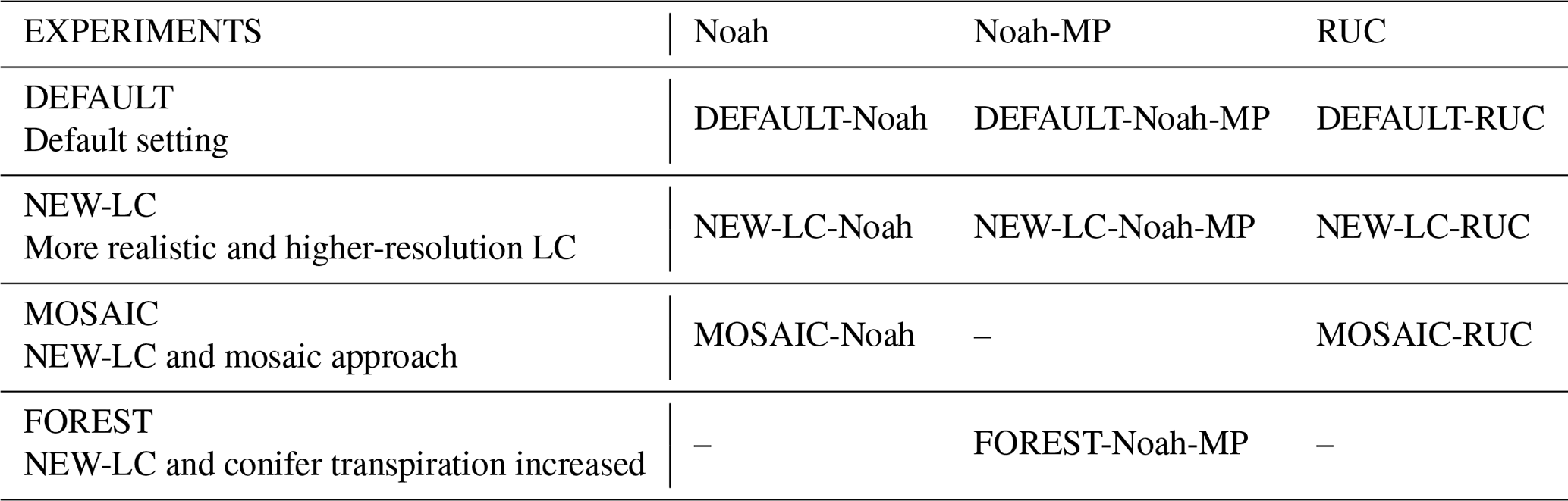
2.3.1 DEFAULT experiment

In this experiment we used the default configuration for the surface representation in WRF, i.e. the LC dataset from IGBP-MODIS (21 categories) and a dominant approach for the sub-grid heterogeneity, which means that the fluxes were calculated taking into account only the surface parameters of the dominant LC category, i.e. assuming that no sub-grid variability exists even when this information is available. The dominant LC category is the one with the highest percentage of coverage within each pixel. This method has an intrinsic dependency on the number of LC categories in the dataset. For example, a pixel with 40 % water, 30 % conifer forest, and 30 % deciduous forest will be treated as water, since it is the dominant category despite both types of forest covering 60 % of the total surface of the grid. On the contrary, the dominant category would be forest if both types of forest were merged into a single category.

It is expected that these simulations will be limited by the fact that the representation of the LC in the area by IGBP-MODIS is not totally correct in comparison with reality (shown later). Also, the dominant approach implies that the model does not take advantage of the higher resolution of the LC datasets.

2.3.2 NEW-LC experiment

In this experiment, we used a more realistic LC dataset than IGBP-MODIS, obtained from 30 m resolution data prepared by CESBIO (Inglada et al., 2017). Figure 2a shows a satellite image of the area evaluated, which serves to visually validate the CESBIO LC at 30 m resolution (Fig. 2b). The inaccurate representation of the pixel-dominant LC by IGBP-MODIS is revealed in Fig. 2c, and the more appropriate surface representation of the dominant LC categories for each pixel used in the NEW-LC experiment is shown in Fig. 2d.

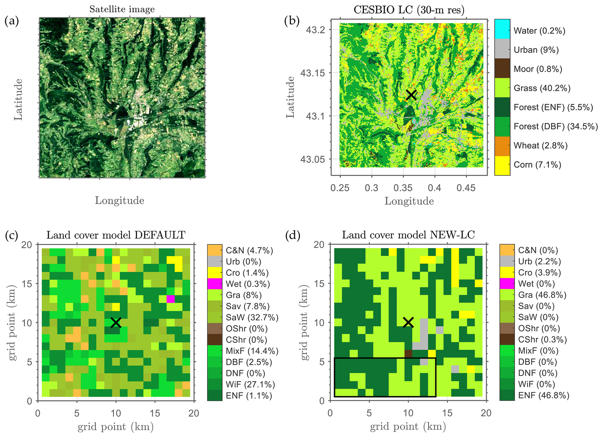
Figure 2 (a) Satellite picture of the area analysed (from © Google Earth, image Landsat/Copernicus). (b) CESBIO land cover map from 30 m resolution data. (c) Dominant land cover (1 km) used in the default experiment (DEFAULT) from the IGBP-MODIS database. (d) Dominant land cover (1 km) used in NEW-LC experiment, obtained from the CESBIO land cover map shown in (b). The black rectangle indicates the area with a soil type dominated by loam, which was not used for the evaluation. The rest of the area was characterized by clay loam (dominantly), as the pixels including the sites where the EC measurements were taken (maximum 4 km away from the central point of the BLLAST field campaign, indicated with a black x symbol). The complete names corresponding to each LC category abbreviation are included in Appendix A.

In order to incorporate the more realistic LC from CESBIO in the WRF model, first, the different categories of the new LC dataset (CESBIO, 17 categories) were transformed into the most appropriate ones of the WRF default LC dataset (IGBP-MODIS). That is, the same 21 LC categories of IGBP-MODIS were conserved, following a similar approach as done in Pineda et al. (2004) and in Schicker et al. (2016). We used the transformations indicated in Appendix A, with some special considerations.

• The two types of forest distinguished by CESBIO (conifer and deciduous) were transformed to conifer (evergreen needleleaf forest, ENF), since the EC measurements used in the AAF were taken over this type of forest due to the lack of measurements over deciduous broadleaf forest. As commented before, the measurements taken over conifers were extrapolated to the areas with deciduous forests in the AAF calculation. By converting all the forest to conifer in WRF, the observation–model comparison was fairer.

• The two possible types of crop in CESBIO (winter and summer crop type, i.e. wheat and corn, respectively) were transformed to the single cropland category available in IGBP-MODIS. Hence, we did not take advantage of the differentiation of crop type by CESBIO, but it is important to note that wheat surfaces only covered 2.8 % of the analysed area (Fig. 2b).

• The four different urban categories in CESBIO were transformed to the single urban definition in IGBP-MODIS. Most of the urban surfaces of the area evaluated were defined as diffuse urban (8.2 %) and industrial zones (0.8 %).

This new LC information was incorporated into the modelling system following the technical details included in Appendix B. Note how even using a more realistic LC dataset over the area, the sub-grid information was not used because the dominant approach was maintained in this experiment.

2.3.3 MOSAIC experiment

Sub-grid heterogeneity is important in the case of the BLLAST area due to the small scale of the LC patches (see Fig. 2b). This makes the area very appropriate for investigating the use of a mosaic approach in the model, as done in the labelled MOSAIC experiment. The mosaic approach implies that the flux is computed for each LC category (tiles) within each grid cell based on the surface parameters tabulated for each one and then averaged taking into account the percentage of coverage of each tile: that is, taking into account the sub-grid surface heterogeneity. In this context, Noah (see Li et al., 2013, for a complete description of the Noah mosaic approach) and RUC allow the possibility of using this approach in the WRF modelling system. The LC improvements of the NEW-LC experiment were also included here. More technical details about the model implementation of this experiment are included in Appendix B.

2.3.4 FOREST experiment

The last experiment was motivated by the large surface flux errors found over pixels covered by conifer (ENF) in previous simulations using Noah-MP. Specifically, this LSM overestimated the SH and underestimated the Le. We hypothesize that this was caused by a parameterized resistance to transpiration that was too high. Hence, we designed the FOREST experiment for Noah-MP. We modified three parameters for ENF with the values used in Bonan et al. (2014).

1. The slope of the Ball–Berry conductance (the inverse of the stomatal resistance to transpiration) equation is the so-called MP in Noah-MP and is usually known as g₁ (the slope parameter). The Ball–Berry equation (Ball et al., 1987) linearly relates the stomatal conductance to the CO₂ assimilation rate:

   $$\begin{array}{}\text{(8)}& g_{\mathrm{s}}=g_{\mathrm{0}}+g_{\mathrm{1}}{A}_{\mathrm{n}}\cdot {\displaystyle \frac{h_{\mathrm{s}}}{c_{\mathrm{s}}}}.\end{array}$$

   In this equation, the slope (g₁) represents the sensitivity of the stomatal conductance to assimilation, CO₂ concentration, humidity, and temperature. It is the parameter that most affects the plant's transpiration (Cuntz et al., 2016), which increases with larger slope values. The g₀ parameter is the minimum conductance, h_s and c_s are the fractional relative humidity and the CO₂ concentration at the leaf surface, respectively, and A_n is the net leaf CO₂ assimilation.

   MP has a default tabulated value of 6 for ENF for Noah-MP, a value that is significantly different compared to the values assigned for other categories (9 for most of them, including, for example, deciduous broadleaf forest – BDF). The lower value for ENF limits the transpiration processes and could be the reason for some of the Le underestimation, leading to more energy being distributed to SH. This parameter was optimized in Bonan et al. (2014), and a value of 9 was also used for ENF in their study.

2. The minimum leaf conductance or the interception in the Ball–Berry equation (g₀, indicated as BP in the Noah-MP scheme) was changed from 0.002 to 0.01 mol H₂O m⁻² s⁻¹, as in Bonan et al. (2014) for ENF.

3. The maximum carboxylation rate at 25 ^∘C (V_cmax25) is a photosynthetic parameter that was changed from 50 to 62.5 $\mathrm{\mu }\mathrm{mol}{\mathrm{m}}^{-\mathrm{2}}{\mathrm{s}}^{-\mathrm{1}}$, as used in Bonan et al. (2014), which is a value also selected according to previous literature. The range of observational values in their work for ENF ranged from 48 to 72 $\mathrm{\mu }\mathrm{mol}{\mathrm{m}}^{-\mathrm{2}}{\mathrm{s}}^{-\mathrm{1}}$, and a value of 62.5 $\mathrm{\mu }\mathrm{mol}{\mathrm{m}}^{-\mathrm{2}}{\mathrm{s}}^{-\mathrm{1}}$ was finally selected.

Hence, these three parameters were modified in Noah-MP according to Bonan et al. (2014), following the technical details included in Appendix B. Indeed, these changes allowed for more evapotranspiration in the ENF forest, which should improve the evaluation in our case study. It should be noted that the g₁ parameter (MP) was the one which most influenced the results, as indicated in Cuntz et al. (2016) and as observed in additional previous experiments performed in our case (not shown). In any case, the objective of this experiment was to demonstrate the high impact of the associated vegetation parameters on the surface fluxes, not the optimization of these values for the specific tree species present in the area analysed here.

2.3.5 Pre-experiments: soil moisture and initial conditions

The previous experiments were performed with initial conditions obtained from NCEP-FNL data (NCEP, 2000) and using the soil moisture initial conditions included in these files (1^∘ horizontal resolution without small-scale details). The impact of these initial conditions has been investigated in two pre-experiments.

One the one hand, the most controversial issue was related to the soil moisture initial value used in the model. Indeed, each LSM used in WRF should be appropriately run for a long time in order to provide appropriate soil moisture values in accordance with the specific LSM dynamics (De Rosnay et al., 2013; Angevine et al., 2014). This should lead to more appropriate (and realistic) initial SM values. However, as commented before, the AAFs used to evaluate the model were based on the assumption of homogeneous soil moisture in the area, similar to the SM field obtained with the 1^∘ resolution of NCEP-FNL. Therefore, in order to perform a fairer comparison of the model with the AAF, the spin-up was not used in our study to avoid the SM horizontal heterogeneity. Also, the simulated soil moisture is, to a large extent, driven by the simulated rainfall, which might be different depending on the LSM used. This can cause undesired differences in the rainfall between the LSM during the spin-up time, which is not appropriate for the comparison performed. However, the impact of performing longer spin-up times was checked in the SPIN-UP pre-experiment (spin-up of 1 month).

On the other hand, we also performed some pre-experiments aimed at quantifying the impact of using different initial condition data. The results obtained with NCEP-FNL were compared to those obtained with ERA-Interim; data from both have a similar horizontal resolution.

The impact of these two experiments related to the previous initial conditions is summarized and discussed in the next section.

3 Results: turbulent flux sensitivity to surface changes

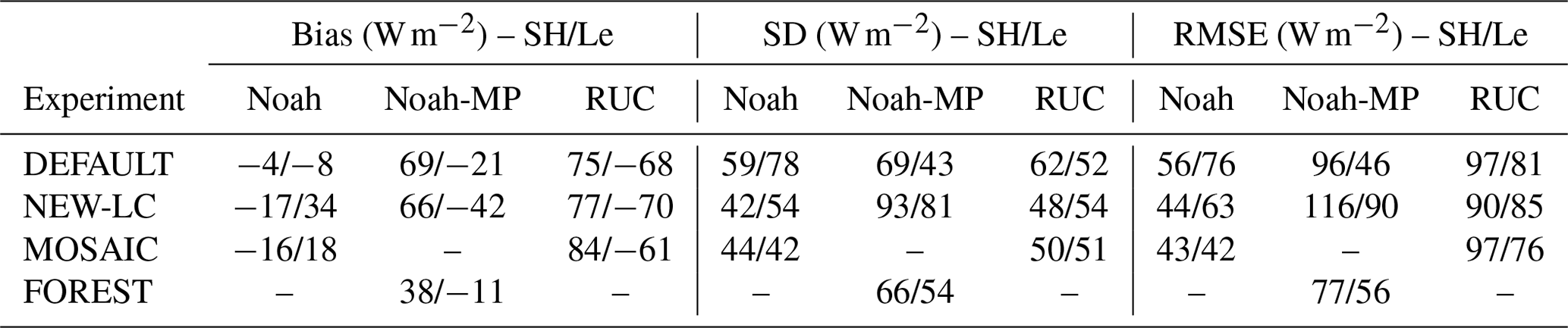
The model skill simulating the AAF fluxes is quantified in this section for the different experiments listed in Table 2. The results are shown and commented individually for each experiment. Since some of the results and the associated discussion differed significantly depending on the LSM used, the results were subdivided for each LSM. As a general reference, Table 3 shows a summary of the total scores (in the whole evaluated area) obtained for SH and Le using the different LSMs and for all the experiments performed.

Table 3 Summary of the scores (W m⁻²) calculated for the evaluated area for each LSM (columns) configured for each experiment (raws). The first value refers to the sensible heat flux (SH) and the second one to the latent heat flux (Le). Some experiments were not possible (–) for some LSMs. The scores used are the bias (systematic error), standard deviation (SD) (random error), and the root mean square error (RMSE).

3.1 DEFAULT experiment versus NEW-LC experiment

3.1.1 Noah

The bias of the simulated SH and Le by the DEFAULT-Noah simulation relative to the observations (the AAF) is shown in Fig. 3a and d, respectively. The results are presented for each LC category, taking into account the dominant LC of each grid cell (1 km) in the model. Note that the DEFAULT experiment includes 10 LC categories in the area based on the IGBP-MODIS database. The total bias values for SH and Le (represented as blue dashed horizontal lines) are close to 0 W m⁻² due to the compensation effect when merging cells with positive and negative biases, but the SD has significant values due to these differences among LC categories, with some surfaces that systematically present noticeable biases. Pixels represented as WiF (wild forest) in the model (27 % of the total area) normally present an overestimation of the SH, while the mixed forest (MixF) pixels (14 %) underestimate it (Fig. 3a). For the Le, the pixels covered by SaW (woody savanna, which represent 33 % of the area) are normally characterized by a remarkable Le underestimation, with bias values around −100 W m⁻² (Fig. 3d).

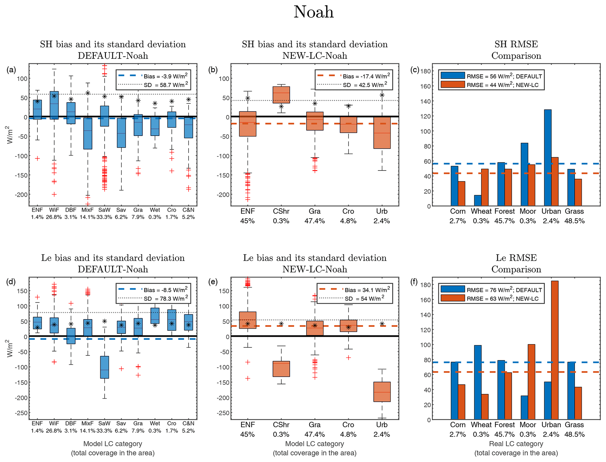
Figure 3 (a) Sensible heat flux (SH) bias box plots by model LC category (x axis) for the default Noah simulation (DEFAULT-Noah). Values are calculated for all the pixels with the specific LC category as dominant in the entire analysed area from 09:00 to 15:00 UTC (hourly values). The standard deviation (SD) is indicated with stars for each LC category. The horizontal coloured dashed line indicates the mean bias in the area analysed, and the black pointed line indicates the SD (these values are also indicated in the legend). The horizontal black solid line indicates the line of 0 W m⁻² bias. The box plots indicate the 50 % of the distribution (from percentile 25 to percentile 75), the upper and lower whiskers the rest of the distribution, and the red crosses the outliers. Note that these figures include the variability due to the number of pixels with the same LC category as the dominant one (variable depending on their coverage) and also the variability due to the 7 h analysed. (b) Same for the results obtained from the Noah simulation with the improved LC (NEW-LC-Noah). (c) SH root mean square error (RMSE) for DEFAULT-Noah and NEW-LC-Noah for each real LC in the area. The horizontal dashed lines indicate the mean RMSE for the whole analysed area. (d–f) Same as (a)–(c) but for the latent heat flux (Le). The percentages included with the x labels refer to those covered by each category with respect to the total evaluated area.

The definition of some of the LC categories existing in the DEFAULT experiment did not appropriately represent the real LC of the area (as seen in Fig. 2c), but they notably influenced the simulated model errors. This is the first indicator of the high dependency of the model results on the LC categories. Then, based on the main hypothesis, the results should improve using a more realistic LC representation (NEW-LC experiment).

The all-area-averaged results for SH and Le from NEW-LC-Noah are shown in Table 3. In this experiment, the LC was modified towards a more realistic representation using the high-resolution data from CESBIO. This led to five LC categories that were present in the area of study as dominant LC, with evergreen needleleaf forest (ENF) and grass (Gra) covering 45 % and 47 % of the total area, respectively. The SH biases observed in the DEFAULT experiment were improved in the NEW-LC, especially for ENF and Gra, with slightly negative (close to zero) values. This led to a slightly negative SH bias in the whole area (Fig. 3b, see the horizontal red dashed line). For the Le bias (Fig. 3e), the opposite is observed, with a slight Le overestimation mainly caused by the Le overestimation over ENF (too much ET simulated by the model in this forest type). As will be shown later, this result contrasts with the findings obtained with the rest of LSMs.

The bias is a good indicator of systematic errors for specific LC categories, but it is a poor indicator of the total model behaviour in the area (it can mix positive and negative values, leading to neutral ones). Hence, the SD and the RMSE have also been included. The SD was also diminished in the NEW-LC experiment, with less variability in the error in the new experiment. In the case of the RMSE (Fig. 3c and f), the results are shown by real LC categories (not model categories), whose fractions of coverage are very similar to those used in the NEW-LC experiment (slightly different due to small differences in the categories; e.g. corn and wheat in the real LC were merged into crop in the model).

The SH RMSE (Fig. 3c) improved for the total area when using the improved LC dataset from 56 W m⁻² (DEFAULT-Noah) to 44 W m⁻² (NEW-LC-Noah). The vertical bars in Fig. 3c indicate the RMSE for each real LC category (the LC categories used in the AAF). They provide information about the types of vegetation associated with larger errors, i.e. vegetation types whose processes or parameters are not well represented by the model. In this case, the SH improvements in the NEW-LC experiment (red bars) are observed for all the pixels except for the only pixel wherein the dominant LC is wheat, associated with a larger SH flux than corn in the observations (see Fig. 2). In any case, wheat crops only covered 0.3 % of the total area as the dominant LC category (one pixel), and therefore the contribution to the total RMSE values was small. The results for Le RMSE (Fig. 3f) also show significant improvements when using the improved LC dataset, except for pixels covered by urban area (with a small impact on the total values due to their scarce presence – 2.4 % – as dominant pixels and for which the results are out of the scope of this work). The Le improvement was more substantial in pixels covered by grass than by forest, since Le is slightly overestimated in the forest pixels (see ENF in Fig. 3e). Notice how, besides the better LC pixel distribution in the NEW-LC experiment, we also avoided using some LC categories associated with large errors in the DEFAULT-Noah experiment, such as the unrealistic SaW pixels related to large Le underestimation (Fig. 3d).

3.1.2 Noah-MP

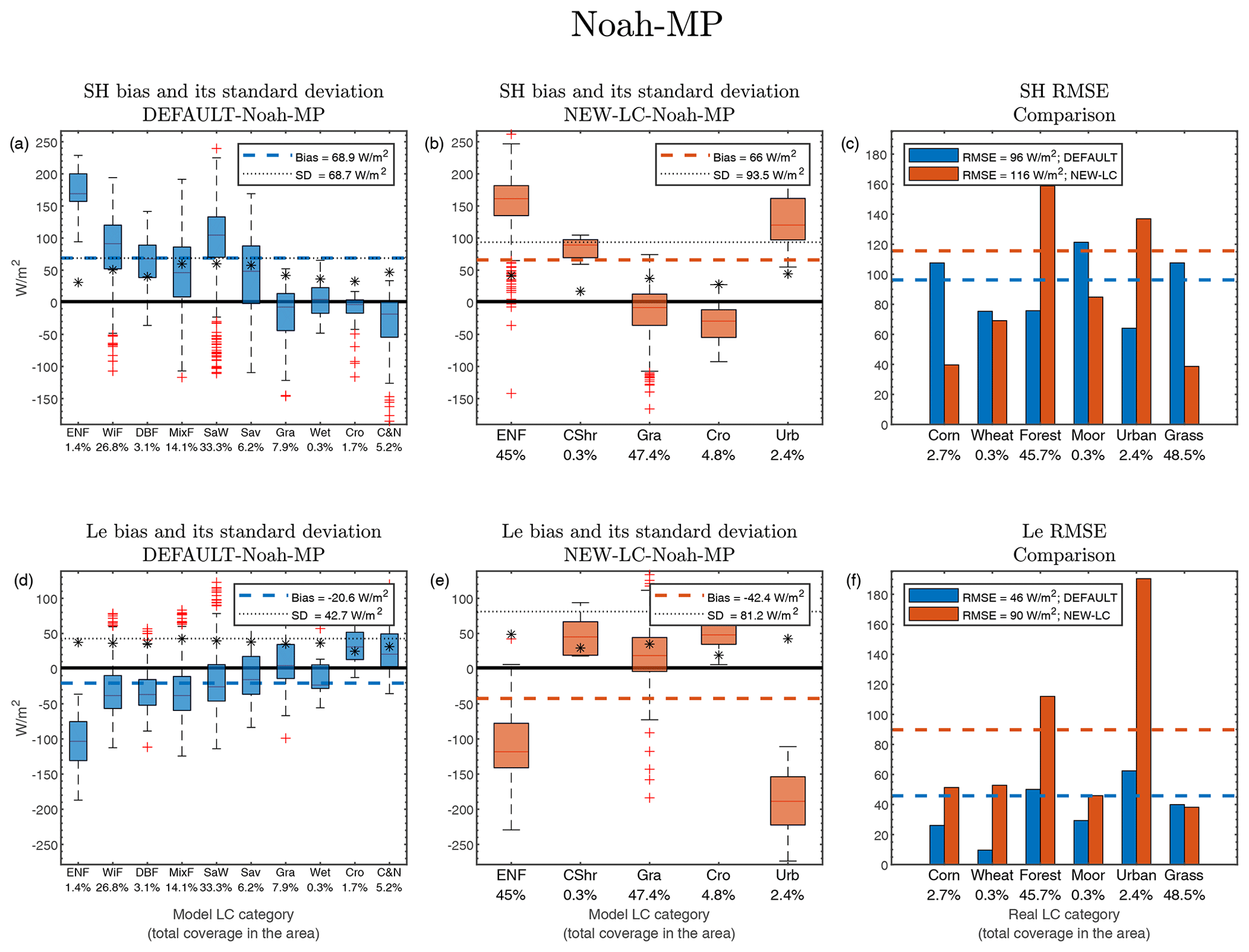
Most of the LC categories showed a positive SH bias for DEFAULT-Noah-MP (Fig. 4a) and a slight negative Le bias (Fig. 4d), especially for pixels whose dominant LC was a type of forest (ENF, WiF, DBF, MixF, or SaW). The SD was the largest for SH and the smallest for Le among the different LSMs (see DEFAULT-Noah-MP in Table 3). This led to a large SH error and to the smallest error amongst the LSMs compared for Le (despite the slight underestimation), with RMSE values of 96 and 46 W m⁻², respectively (see Fig. 4c and f and also Table 3).

Contrary to what happened with Noah, the results were generally (all area) worse in the NEW-LC experiment, even for the case of SH in which the RMSE was already high. The SH bias remained positive, mainly influenced by the significantly high SH bias in ENF pixels (more than +150 W m⁻²), while the biases over the grass and crop pixels were close to zero (Fig. 4b). For the Le, important negative biases were observed in pixels mostly covered by ENF (around −120 W m⁻²), but with lower errors for grass or crop pixels. The contrasting differences among the biases for the two more common LC categories (grass and forest) led to high values of SD. The urban pixels were characterized by important biases, but their small proportion as the dominant LC category led to a small contribution to the total error.

This error variability among categories and the fact that the 45 % of the total area was covered by ENF led to final RMSE values of NEW-LC-Noah-MP (horizontal red dashed line in Fig. 4c) significantly higher than those of DEFAULT-Noah-MP (shown in blue), increasing the total SH RMSE up to 116 W m⁻² and the Le RMSE up to 90 W m⁻², with a significant worsening for the forest and urban pixels. However, the bars in Fig. 4c and f also illustrate the improvement in the crop, moor, and grass pixels for SH and grass for Le, but they were not enough to compensate for the large errors found over the ENF pixels. This was not observed in the Noah experiment (previous subsection), which uses a different set of vegetation parameters than Noah-MP for each LC category. This suggests that the biased results for Noah-MP could be partially caused by some vegetation parameters that were inappropriate for the ENF LC category, which is a hypothesis investigated later in the FOREST experiment.

Figure 4 Same as in Fig. 3 but for Noah-MP.

3.1.3 RUC

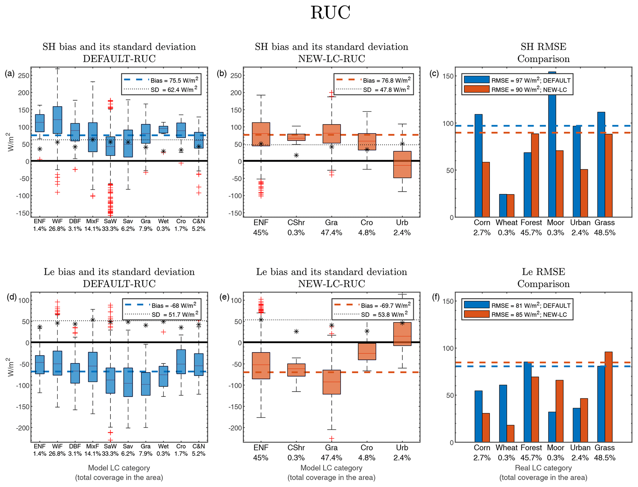
The SH and Le biases obtained when using the DEFAULT-RUC simulation are the highest ones among the compared LSMs (see comparative Table 3), while the SD values are similar to the other LSMs. Hence, RMSE values of 97 and 81 W m⁻² for SH and Le, respectively, were obtained for the DEFAULT-RUC simulation. There is a systematic SH overestimation for all the LC categories (Fig. 5a) for DEFAULT-RUC, which is especially aggravated by pixels unrealistically represented by WiF (Wild forest), with a bias of more than 100 W m⁻² covering an important fraction of the total analysed area (27 %). The Le is systematically underestimated (Fig. 5d) for all the LC categories, which shows a tendency towards too little ET in this LSM in this studied case, especially in LC categories with shorter vegetation (SaW, Sav, and Gra).

These biases, the SD, and the RMSE values were very similar in the NEW-LC-RUC experiment using the more realistic LC, with SH RMSE of 90 W m⁻² and Le RMSE of 85 W m⁻². The values obtained for each LC category (Fig. 5b and e) were within the same order of magnitude as those obtained in the DEFAULT-RUC experiment or even higher, as is the case of the SH simulated in grass surfaces, with a remarkable overestimation of around +75 W m⁻². This led to very similar (and high) RMSE values for the DEFAULT and NEW-LC experiments (Fig. 5c and f). Although the SH simulation improved for the grass and corn pixels, it worsened for the forest pixels. For the Le, the opposite was observed: the biases of the forest and crop pixels improved but worsened for the grass ones, which were associated with ET that is too low. Note how the RMSE in the NEW-LC experiment over grass surfaces was higher than 100 W m⁻² in RUC, while it was around 40 W m⁻² in the rest of the analysed LSMs for which grass surfaces were normally associated with improvements.

Although it is not shown in this work, we detected a higher sensitivity of this LSM to the soil type in comparison with the other LSMs. Thus, the parameters associated with clay loam could be inappropriate for this LSM, leading to a wrong partitioning of the net radiation in the model (Le that is too low and SH that is too high). In contrast, the sensitivity of RUC to the LC categories was the lowest one among the compared LSMs. In any case, the analysis of the relative contribution of the soil type to the surface fluxes is out of the scope of this study. In addition, the soil moisture values used to initialize this LSM should be corrected due to its different SM dynamics and baseline (see the discussion included for the pre-experiments in Sect. 3.5).

Figure 5 Same as in Fig. 3 but for RUC.

3.1.4 NEW-LC experiment overview

In general, the simulation of the fluxes in the NEW-LC experiment improved over pixels mostly covered by grass and crop. However, the specific analysis from previous subsections revealed how changing the LC representation in the model towards a more realistic one (NEW-LC) did not necessarily lead to an improvement of the fluxes in the whole analysed area for all the LSMs. In Noah-MP, this was mainly caused by the errors found in the pixels mostly covered by coniferous forest (ENF), for which the simulated values of the fluxes were extreme (overly positive SH bias and negative Le bias). This notably impacted the scores over the analysed area due to the high percentage of pixels wherein the dominant LC was forest (46 %). Noah-MP includes more and different parameters associated with this vegetation type, an aspect that will be investigated later in the FOREST experiment. In contrast, Noah is the LSM least affected by errors in the conifer forest, and, indeed, it is the LSM that most improves the simulation of the surface fluxes in the NEW-LC experiment.

This is clearly observed in Fig. 6, where the SH and Le at 12:00 UTC for the different dominant LC categories (colours) are plotted against the fraction covered by the dominant LC category within each pixel. Panels (a) to (c) (SH) and (e) to (g) (Le) show the simulated values for the different LSMs, while panels (d) and (h) show the observed values from the AAF for comparison. The dependency on the fraction of the dominant category is clearly observed for the AAF in Fig. 6d (SH) for forest and grass pixels: the higher the percentage of forest, the higher the SH, since forests were associated with the highest values of observed SH. The opposite is observed for the grass pixels, with SH diminishing for increasing percentages since grass EC measurements showed the lowest SH values. These dependencies are slightly observed for the Le (Fig. 6h, Le) due to the similar Le values measured over all the surface types with the EC towers (see Fig. 1b and d). Coming back to Fig. 6, one can deduce that Noah is the LSM that provides the most realistic values in comparison with the AAF from a visual comparison, especially for Le.

The other LC category associated with large biases was the urban one. In this case, the effect on the scores of the total area was minimal, since only 2.4 % of the pixels have urban area as the dominant LC category. As commented before, a fair discussion about the absolute values of the errors found over this type of LC is out of the scope of this article due to the relatively high uncertainties in the AAFs and the lack of a specific urban parameterization in the model, with values for Noah and Noah-MP that are too extreme: 0 W m⁻² for Le; see the grey circles in Fig. 6e and f.

Furthermore, the dependence of the AAF with the percentage of coverage of the dominant LC in each pixel is clearly observed in Fig. 6d and h, which is inherent to the methodology used in the AAF calculation. However, this dependence is hardly seen from the model outputs (as expected using the dominant approach; note the small slope of the scatter plots for each coloured category). As commented before, it should be noted that, by default, these LSMs use a dominant approach for each grid cell with only some surface information (LAI, roughness length, or albedo) from the dominant LC (Li et al., 2013). This led to well-differentiated flux values for each category (Fig. 6).

Hence, from the NEW-LC experiment, we can conclude that there is a high dependence of the fluxes on the LC type in WRF, which can lead to important biases if the parameters and processes associated with specific categories (conifer forest in this case) are not appropriate. These results agree with those found by Couvreux et al. (2016), wherein 12 IOPs of the same field campaign were simulated with the ARPEGE (Courtier and Geleyn, 1988), AROME (Seity et al., 2011), and ECMWF models (Simmons et al., 1989), with grid sizes of 10, 2.5, and 16 km, respectively. In this work, the SH was systematically overestimated over the area analysed by the three models. Indeed, a larger SH overestimation was found for the ARPEGE model in two of the three evaluated pixels close to the area, the surface of which was represented as forest. This also highlights the issues found over this type of vegetation cover, which was enhanced with a dominant approach (as in WRF in this work and in AROME in Couvreux et al., 2016). This simplified approach does not take advantage of the available sub-grid surface information and motivated the MOSAIC experiment, for which the sub-grid heterogeneity was taken into account in the Noah and RUC models.

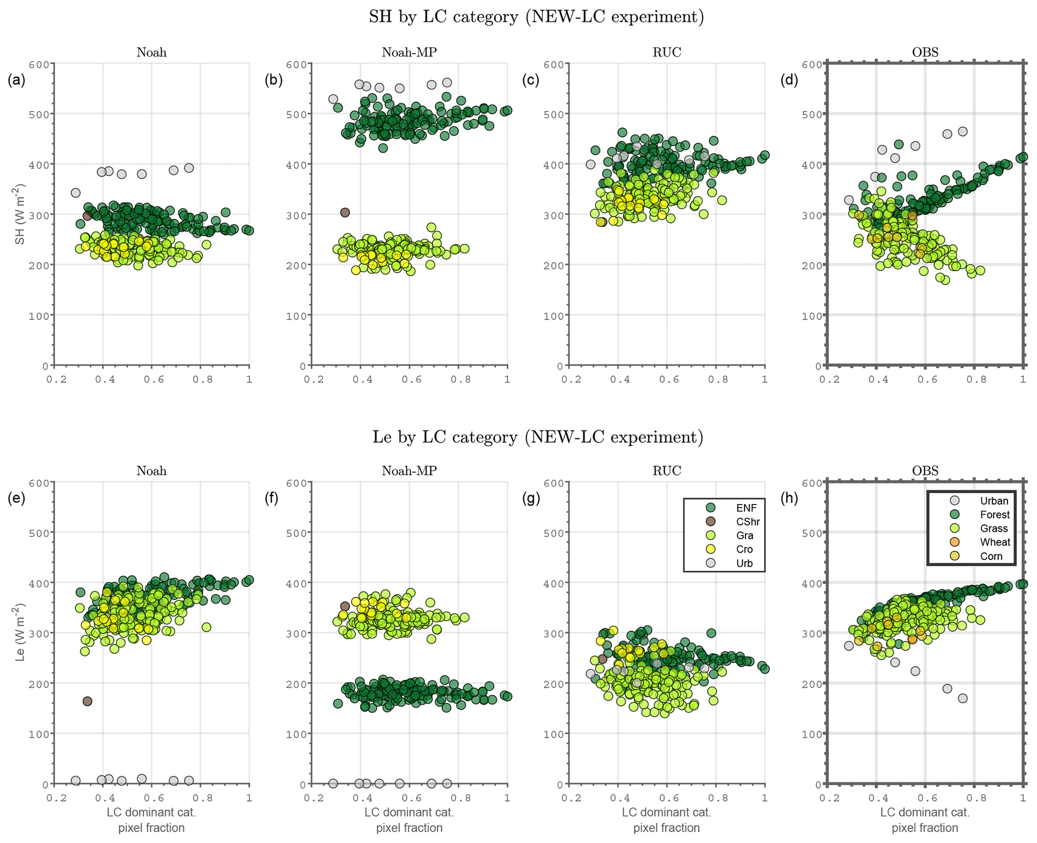
Figure 6 SH (a–d) and Le (e–h) simulated at 12:00 UTC by each LSM: Noah (a, e), Noah-MP (b, f), and RUC (c, g). The x axis shows the total fraction covered by the dominant LC category in each respective pixel. The results are provided for the different LC categories with colours. Panels (d) and (h) represent the same but for the gridded area-averaged fluxes (AAFs) calculated from the EC measurements, which are used for the model evaluation.

3.2 MOSAIC experiment

The scores obtained using the mosaic approach in the Noah and RUC LSMs are shown in Table 3, with significant improvements in comparison to the NEW-LC experiment in Le. For Noah, a reduction of almost 20 W m⁻² in the Le RMSE (from 63 to 45 W m⁻²) was observed as a result of a decrease in the bias and in the SD. For RUC, the improvement in the Le RMSE was of 9 W m⁻². The SH scores are nearly unmodified in Noah and worse in RUC-MOSAIC.

For the case of Noah, Fig. 7 shows the simulated SH and Le obtained from the NEW-LC and MOSAIC experiments. The use of the mosaic approach (panels b and e) caused a merging effect among values from different categories on the simulated fluxes in comparison with the dominant one (panels a and d), with results that better resemble the figures obtained from the AAF (panels c and f). This is particularly clear for SH, for which the stronger dependence of the fluxes on the type of dominant LC (Fig. 7a) is removed in the mosaic approach (Fig. 7b). The impact was larger on pixels wherein the dominant LC was forest, which were associated with more extreme flux values. Also note the nearly zero values of Le in the dominant approach in urban pixels (panel d) and the Le values that depend on the fraction of urban area within each pixel (panel e). The correlations of the fraction of coverage of the dominant LC category and the surface fluxes are included in the legend for each LC category in Fig. 7. This correlation depends on the strength of the flux values associated with the specific categories. For example, the anti-correlation observed in Fig. 7e for the urban pixels is due to the strong impact when increasing the percentage of cover of this LC category. Thus, if a pixel with 100 % urban area were present, its Le value would tend to 0 W m⁻² using a mosaic approach, as observed when using the dominant method in Fig. 7d.

However, this merging effect was only slightly observed for the case of the MOSAIC experiment in RUC (Fig. 8). This was probably caused by the fact that the mosaic approach used in RUC is applied for different variables than in Noah. In the case of RUC, only average emissivity, LAI, roughness length, and plant resistance are calculated based on the percentage of each land cover. In RUC, the averaged albedo, which is the parameter that has the highest impact on the net radiation of each grid cell, subsequently affecting SH and Le, is not used. Figure 9 shows the albedo differences between NEW-LC and MOSAIC used by the Noah (upper figures) and RUC models (bottom figures). While the values for MOSAIC-Noah (Fig. 9b) consisted of a weighted average from the different LC of each grid cell, it was not the case for MOSAIC-RUC (Fig. 9d), which diminished the impact of the mosaic approach application in the RUC model.

Adding a mosaic approach caused a change in the LC percentage technically used for some LC categories. This is clearly observed in the comparison of the percentages shown in Fig. 1b and d. For example, 2.2 % of the pixels were characterized as urban with the dominant approach (panel d), while the coverage using a mosaic approach increased up to 9 % (panel b). In this case, the mosaic approach increases the percentage of urban fluxes contributing to the averaged values, although in a much more diffuse way (concentrated in more pixels). However, the extreme effect of pixels considered fully urban is removed. This is also the case for the crop pixels that cover 9.9 % of the area (wheat and corn) shown in Fig. 1b (taking into account the sub-grid variability), but only 3.9 % as the dominant category in 1×1 km pixels (Fig. 1d).

In any case, the mosaic approach might always be more realistic than the dominant one; in the latter, the sub-grid information is not used and a unique LC type is defined, even when the combination of secondary and similar LC categories has a higher percentage than the dominant one (e.g. 40 % conifer, 30 % dense shrub, and 30 % open shrub). If the resulting dominant category is associated with inappropriate parameters (e.g. conifer in the example and in our case), the error will be greater in the dominant approach. For this reason, it is also crucial to be cautious with some LC definitions that could lead to fluxes that are too extreme. This can have an important impact on the results of the simulations, either with a dominant or a mosaic approach, as stated in Mallard and Spero (2019). Furthermore, appropriate flux measurements for model evaluation over urban surfaces still remain a challenge, and the LSMs present issues without an additional urban parameterization included, which is an aspect that should be better analysed in future studies.

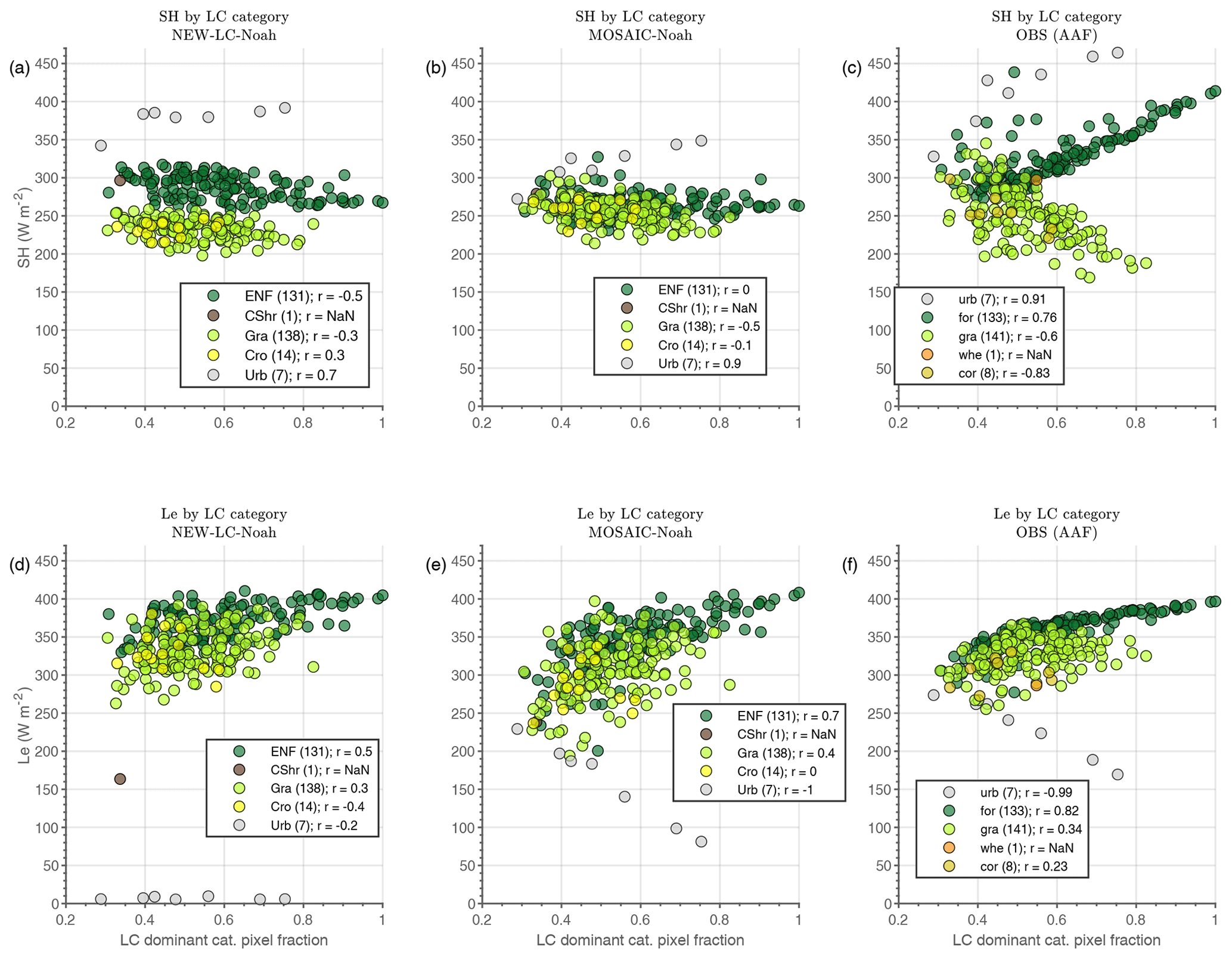
Figure 7 Same as in Fig. 6 but comparing the results from Noah-NEW-LC (using a dominant approach) and from Noah-MOSAIC (using a mosaic approach). Panels (c) and (f) correspond to the area-averaged fluxes (AAFs) from observations, which are considered to be the reference. The correlation between the fluxes and the fraction of coverage of the dominant LC category is included in the legend for each LC category within each pixel, with the number of pixels used in brackets.

Figure 8 Same as in Fig. 7 but for NEW-LC-RUC (dominant) and MOSAIC-RUC (mosaic).

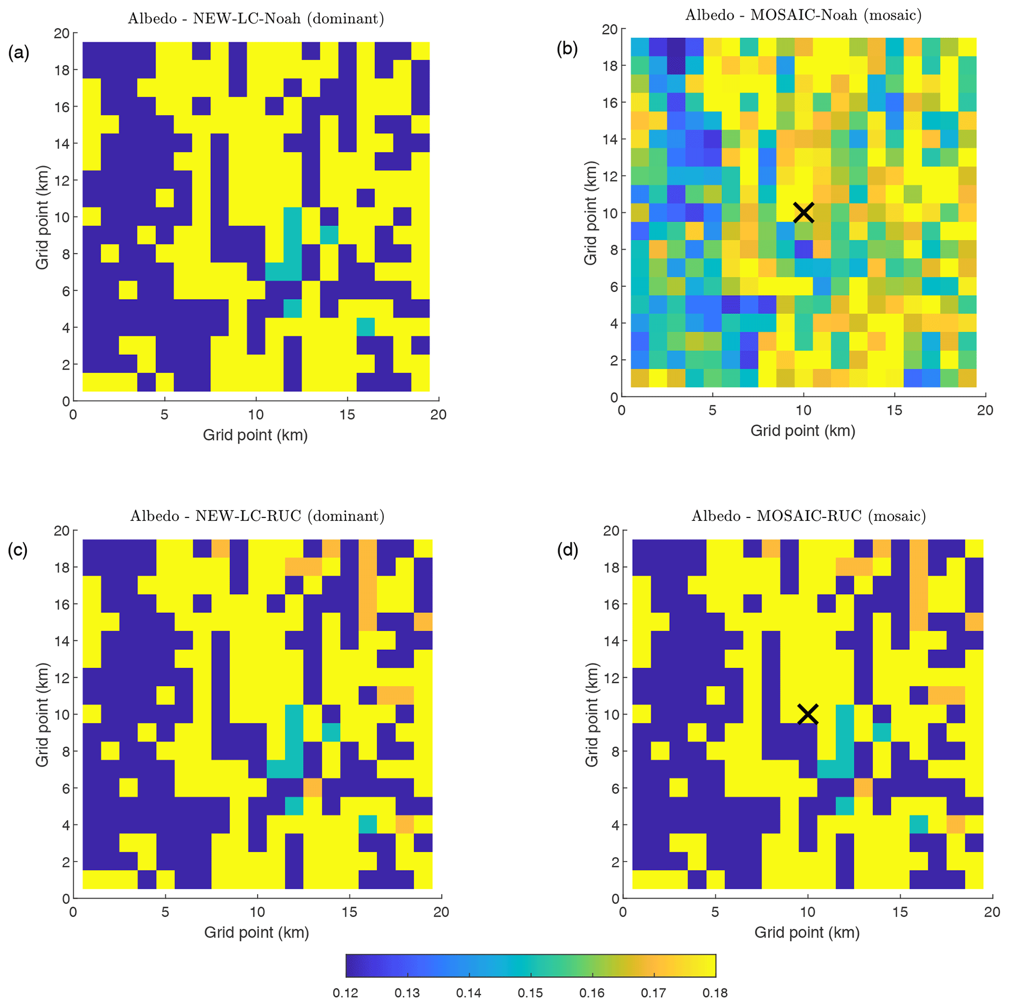
Figure 9 Model albedo over the analysed area. Comparison of the grid values between the dominant (a, c) and the mosaic (b, d) approaches for Noah (a, b) and for RUC (c, d). Note the absence of change in the mosaic approach using RUC.

3.3 FOREST experiment

The previous experiments revealed the large biases in simulated surface fluxes associated with conifer forests (ENF) for Noah-MP, with overly low simulated values of Le and overly high SH in comparison with the observed values (Fig. 6). This was also the case for RUC (Fig. 6d and i), but in this case the biases were not limited to the ENF pixels and also extended to all the categories.

Since the biases were only observed in ENF for Noah-MP, we hypothesize that this was caused by overly high resistance to the transpiration parameterized for these type of trees. We explained in Sect. 2.3.4 the motivation for this experiment and we justified the changes applied based on the parameter values used in Bonan et al. (2014) for ENF. Specifically, we changed the values of the g₁, g₀, and V_cmax25 parameters. These modifications should lead to increased transpiration and therefore also to decreased SH. Indeed, this is observed in the results: the RMSE decreases to 77 W m⁻² for SH and to 56 W m⁻² for Le, which are lower errors compared to the NEW-LC-Noah-MP experiment (see Table 3). This was the result of an improvement in the systematic error found in the ENF pixels due to the reduction in the extreme biases found in ENF. Specifically, the ENF mean bias reduced from +156 to +85 W m⁻² for SH and from −110 to −32 W m⁻² for Le when comparing the NEW-LC and the FOREST experiments (these results are not shown in figures), while the SD values remained similar, illustrating how we improved the systematic bias associated with this LC type due to incorrect parameters related to the evapotranspiration of these trees in this case study.

The results are consistent with the fluxes shown in Fig. 10, where the SH and the Le observed at the forest site (black line) were compared to the simulated values obtained with the central pixel of the domain completely (100 %) covered by ENF (conifer, blue) or by ENF with these parameters changed (red line). These two additional simulations shown in Fig. 10 would correspond to the NEW-LC Noah-MP and the FOREST Noah-MP experiments, respectively. However, in these graphics the effect of the change is analysed in a clearer way for the whole diurnal cycle. Again, it is demonstrated how the tuning of these parameters towards less resistance to transpiration provided better results than the original parameters tabulated for ENF for both SH and Le. The slope of the Ball–Berry equation (g₁) is the parameter that most influenced the results, which does not seem appropriate in this area for this type of tree, since it limits transpiration too much. As asserted in Medlyn et al. (2011), g₁ is the key parameter for plant stomatal conductance, being quite variable among species in areas with different environmental conditions. The authors suggested that g₁ should increase with increasing temperatures, as might be the case in our study, compared to the values tabulated for this LC category in the model. The results of the present work indicate that the tabulated values, which were developed for other region and dates or even with a different type of conifer or density of trees, should be revised. This is consistent with the scientific demand for systematic experimental observations representative of different scales (Vilà-Guerau de Arellano et al., 2020) from the leaf level (as stomatal conductance) to the landscape and model grid scales (for example, reliable area-averaged fluxes).

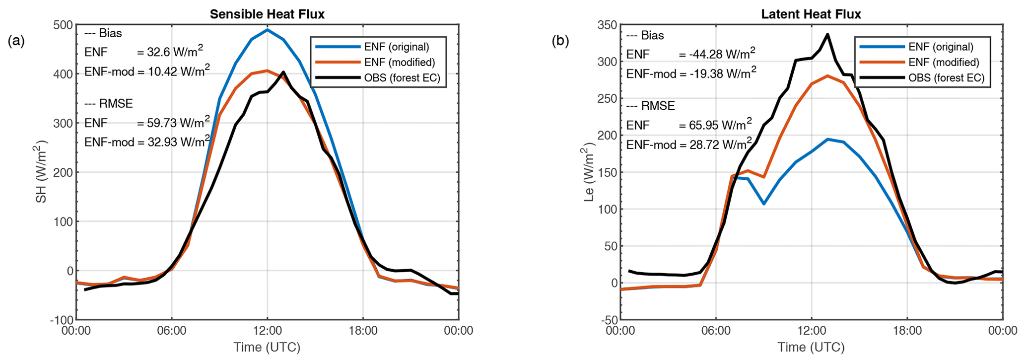
Figure 10 (a) Sensible heat flux (SH) from two simulations with the evaluated pixel completely covered by the original ENF (conifer, blue) and ENF-mod (conifer with parameters modified, red). The observations made over the forest site are indicated with a black line. (b) Same for the latent heat flux (Le). The model results were obtained using the Noah-MP land surface model for 19 June 2011. The biases and root mean square error (RMSE) are included.

3.4 Analysis of the simulated evaporative fraction (EF)

The previous analyses provided information about the biases and the RMSE of SH and Le independently for the different experiments and LSMs. However, these analyses did not take into account the total energy available to be partitioned into the atmospheric fluxes, which may be different depending on the surface type. Hence, in Fig. 11 we present the evaporative fraction ($\text{EF}=\text{Le}/(\text{Le}+\text{SH})$) for each LSM (panels) sorted by the real LC categories of each grid cell for the different experiments performed (DEFAULT in blue, NEW-LC in red, MOSAIC in orange, and FOREST in green). The values obtained from the AAF are also included as a reference in dark grey in the different panels. The highest observed values were in pixels with grass as the dominant LC, while in the forest ones the EF was around 0.5. The values observed from the EC towers (representing a homogeneous surface) are indicated with black circles and represent what would be expected in a pixel completely covered by each LC category. For example, EF is 0.73 for grass surfaces and 0.45 for forest ones.

In Noah (Fig. 11a), the DEFAULT experiment (blue) provided a large variation in the EF of each real LC category. This resulted from the unrealistic and varied LC representation in this experiment. The NEW-LC experiment (red) partially corrected the large EF variability, especially for the grass and forest pixels. Therefore, in general, not only were the SH and Le biases corrected, but also the flux partitioning, except for the moor and urban pixels with a scarce presence. In addition, the MOSAIC experiment (in orange) served to improve the simulated values of EF, which were very close to those obtained from the AAF.

The DEFAULT experiment in Noah-MP (Fig. 11b) systematically underestimated the EF (blue) in comparison to the observations (dark grey). The NEW-LC experiment (red) served to correct this underestimation in all LC categories except in the forest and urban grid cells. As discussed before, the Le was significantly underestimated in the forest (ENF) pixels, while the SH was overestimated, which led to underestimation of EF. This was partially corrected in the FOREST experiment (represented with green in Fig. 11b) by applying modified parameters that made transpiration easier from these plants. However, even with these changes, the EF values obtained from the model were far from those from the observations.

RUC (Fig. 11c) exhibited the smallest sensitivity to the modifications performed in each experiment in comparison to the other LSMs. As commented before, the LC changes in RUC had a lower impact on the results, which were more impacted by the soil type (not shown) than by LC. Hence, RUC showed a general tendency to underestimate EF with systematic Le underestimation and SH overestimation for all the LC categories, as was previously observed.

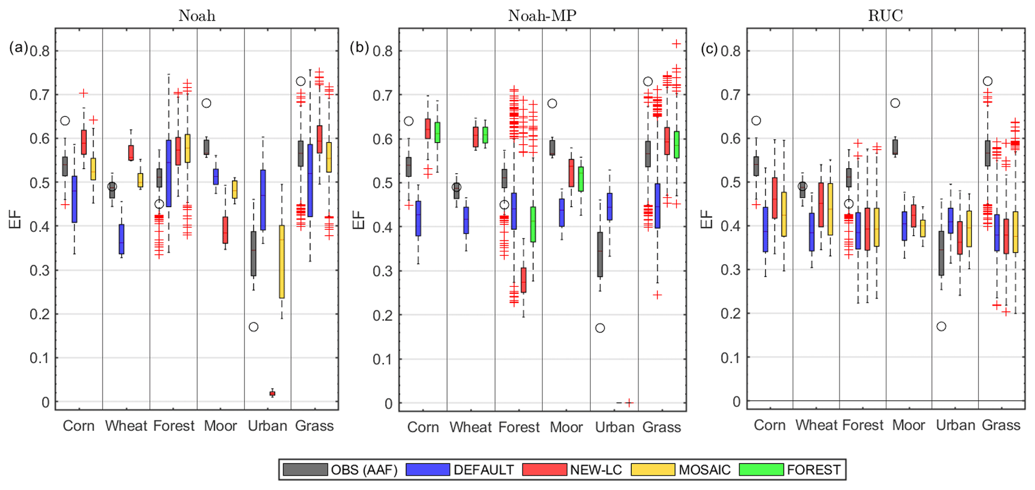
Figure 11 Evaporative fraction ($\text{EF}=\text{Le}/(\text{SH}+\text{Le})$) for the different LSMs used: (a) Noah, (b) Noah-MP, and (c) RUC. The results are ordered by the real dominant LC type of the pixels (vertical subdivisions) and for the different experiments performed: DEFAULT (blue), NEW-LC (red), MOSAIC (orange, only in Noah and RUC), and FOREST (green, only in Noah-MP). The values obtained from the observations (AAF) are indicated with dark-grey box plots. Black circles indicate the EF obtained from the EC towers for each corresponding (homogeneous) surface.

3.5 Pre-experiments (initial conditions)

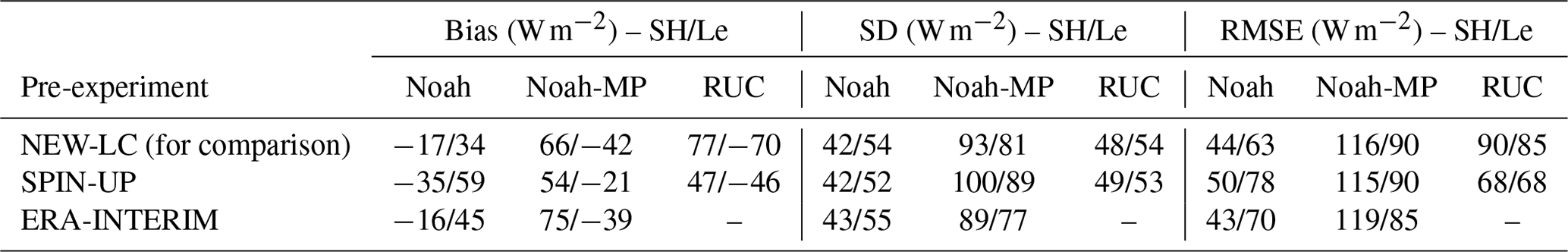
As commented in Sect. 2, the impact of the data used to initialize the model has also been investigated and quantified. These are named pre-experiments because their impact is mainly limited to the initial values used to initialize the model (i.e. they do not alter surface parameters that affect the whole simulation as in the experiments analysed before). Two pre-experiments were designed: (1) SPIN-UP, in which the WRF model was run with each LSM for a longer time (1 month) before the analysed period, allowing us to obtain SM values more appropriate for the specific dynamics of each LSM; and (2) ERA-INTERIM, in which the WRF model was initialized with a different set of initial and boundary condition data from ERA-Interim (ERA-Interim, 2009). Note how in this case the boundary conditions can have a small impact every 6 h in the simulation, not only at the starting time (boundary conditions). The rest of the model configuration of these experiments was the same as in the NEW-LC experiments; therefore, their scores are compared in Table 4 to those obtained with the NEW-LC experiment (using initial conditions from NCEP-FNL and no spin-up time).

Table 4 Summary of the scores (W m⁻²) calculated in the whole evaluated area for each LSM (columns) configured for each pre-experiment (raws, SPIN-UP, and ERA-INTERIM). The scores of the NEW-LC experiments are included to quantify the impact of the change in the initial conditions. The first value refers to the sensible heat flux (SH) and the second one to the latent heat flux (Le). Some experiments were not possible (–) for some LSMs. The scores used are the bias (random error), standard deviation (SD) (systematic error), and the root mean square error (RMSE).

3.5.1 SPIN-UP experiment

With the SPIN-UP experiment, we have checked the LSMs' sensitivity to auto-spin up their SM values by performing longer simulations (1 month before the model output is used and analysed). As discussed before, in our case this was not appropriate to allow a fairer model–observation comparison (the AAFs used to evaluate the model were based on the assumption of homogeneous SM, which does not exist after the spin-up time). Also, the inherent differences between the LSMs cause variations in the rainfall simulated by WRF in each LSM, which make the comparison of the LSMs' scores difficult (Anonymous, 2021).

The analysis of the scores obtained from the SPIN-UP experiment in Table 4 reveals that the biases worsened for Noah (from −17 to −35 W m⁻² and from 34 to 59 W m⁻² for SH and Le, respectively), while the SD values were similar, leading to a larger RMSE for both fluxes. For Noah-MP the bias was corrected (from 66 to 54 W m⁻² and from −42 to −21 W m⁻² for SH and Le, respectively), but at the expense of an increase in the SD, which led to similar RMSE values. This LSM showed biases with a different sign depending on the LC category (see Fig. 4), especially for forest (SH overestimation and Le underestimation) and grass (the opposite), which led to a mean bias value that should be analysed with caution: the value for the whole area, as shown in Table 4, includes compensating errors the can lead to erroneous conclusions. In the case of RUC, the SPIN-UP experiment improved the biases for both fluxes (from 77 to 47 W m⁻² and from −70 to −46 W m⁻² for SH and Le, respectively), while the standard deviation of the error is the same, leading to a substantial reduction of the RMSE. Indeed, this was suspected in Angevine (2021) since the RUC model has a different baseline and dynamics for the soil moisture than Noah, Noah-MP, and the NCEP-FNL data (based on Noah). In this case, leading the model to auto-spin up some time is convenient, since the fluxes simulated by this LSM improved with their RUC-specific SM values. Hence, the SM initial value for RUC should be higher than for Noah (in this case study), which corrects the Le underestimation and the SH overestimation observed in Fig. 5.

3.5.2 ERA-INTERIM experiment

Not only can the SM have an important effect on the model results, but the rest of the atmospheric variables used to initialize the model can also impact the whole simulation. This possibility was studied using a different database to initialize the model (ERA-Interim versus NCEP-FNL). The comparison of the scores obtained with the ERA-INTERIM experiment slightly affects the evaluation: in Noah the bias changed from −17 to −16 W m⁻² for SH and from 34 to 45 W m⁻² for Le, leading to similar RMSE values. In the case of Noah-MP, the bias varied from 66 to 75 W m⁻² for SH and from −42 to −39 W m⁻² for Le, also with similar RMSE values. Therefore, although there is an impact of the initial conditions on the evaluation of the model, in this case the effects were not very large. Nonetheless, using other datasets with higher resolution (as ERA-5) could lead to improvements due to the improved resolution used at the model initialization, but additional experiments aimed at investigating the impact of the resolution of the data used to initialize the model are out of the scope of this article.

4 Summary and conclusions

The changes in the LC of the Earth's surface trigger varied and sometimes unpredictable consequences at different spatiotemporal scales, affecting biophysical processes in the soil and in the atmosphere. Hence, it is crucial to know more about the impacts of the LC changes on all these processes. In this work, we investigated the sensitivity of turbulent heat fluxes simulated by the WRF model to the manner in which the surface is represented in it.

To this aim, different sensitivity experiments were performed for a case study over a heterogeneous area in the south of France. They were evaluated with gridded area-averaged fluxes (AAFs) computed from tower measurements installed over five vegetation types (forest, corn, wheat, grass, and moor) during the BLLAST field campaign. In order to add robustness to the study and to detect differences, the experiments were carried out using three LSMs available in WRF: Noah, Noah-MP, and RUC.

First, a control experiment was performed with the default options in WRF: LC from the IGBP-MODIS database and a dominant sub-grid approach; i.e. the model used the tabulated surface parameters of the LC category with the highest percentage of coverage in each pixel. We hypothesized that these simulations were limited because of the large differences between the LC representation and the actual surface and because of the loss of LC information at the sub-grid scale.

Thus, a new experiment was designed (named NEW-LC) that improved the surface representation by adding the LC information from the 30 m resolution CESBIO maps, which were much more accurate and realistic in the area than the default IGBP-MODIS dataset. The observed changes in the surface fluxes were dependent on the LSM used due to their differences in the parameters associated with each vegetation type and also to their different representation of the surface processes. The improvement was clear for Noah for all the LC categories. RUC was the LSM that showed the weakest response of the fluxes to the LC categories, without substantial changes in the scores. Noah-MP showed some improvements in pixels covered by crops or grass, but they also exhibited an important SH overestimation and Le underestimation in the surface fluxes simulated over pixels mainly covered by conifer forest (ENF). The ENF biases contributed significantly to the total model error due to their relatively high percentage of coverage (45 %) in the analysed area. The NEW-LC experiment revealed the need for a correct representation of LC in the analysed area, in part due to the high dependency of the fluxes on the LC categories. In addition, the appropriate characterization of surface parameters associated with some LC categories (e.g. conifer) still needs to be improved, as was also discussed in previous works (e.g. Li et al., 2013; Cuntz et al., 2016).

In the second experiment (named MOSAIC), the sub-grid heterogeneity (below 1 km) was taken into account with a mosaic approach in Noah and RUC, meaning that the fluxes in each grid were calculated as weighted averages from individual surface fluxes obtained from each tile or LC category. The mosaic approach caused more homogeneity among the surface fluxes simulated in the analysed pixels, which corresponded better to the AAF used as benchmark data. This improvement in the surface representation led to improved scores for Noah (especially for Le), while smaller changes were observed in RUC. This was because in RUC the mosaic approach did not include the use of pixel-averaged albedo values based on the percentages of each LC category, as done for the surface roughness, LAI, and emissivity. In Noah, the albedo was also averaged, significantly contributing to the improvements, since the albedo is the parameter that seems to have a larger impact on the net radiation available to be partitioned into SH and Le.

Finally, a last experiment (named FOREST) was motivated by the issues found in the conifer pixels for Noah-MP. The modifications in the FOREST experiment were conducted to reduce the resistance of conifer trees to transpiration using updated parameters as used in Bonan et al. (2014). The effect of these changes was to facilitate transpiration processes, coinciding better with the observations and improving the scores.

Two additional pre-experiments aimed at checking the model sensitivity to the initial conditions were performed. In the first one, a spin-up period of 1 month was applied for each LSM in order to obtain more appropriate SM values for each pixel. This was very important for the case of RUC since the SM in this LSM has different dynamics and a different range of values than Noah, Noah-MP, and the SM from NCEP-FNL, leading to improved scores with a corrected SM value. In the second pre-experiment the sensitivity to the initial conditions was checked by comparing the NCEP-FNL results with those using ERA-Interim, with a slight impact on the simulation scores.

This work demonstrates the importance of a correct representation of LC in the area which is evaluated, as was also shown in previous works (Cheng et al., 2013; Schicker et al., 2016; Jiménez-Esteve et al., 2018). This can considerably affect the simulation of the fluxes that will drive the associated boundary-layer processes. Also, it is worth using a mosaic approach to benefit from the sub-grid surface information that is normally available.

In any case, the particular conditions of the region and dates analysed mean that some specific conclusions might not be applicable to other regions or even to the same region under different conditions. For example, it is also possible that in our case we observed more ET over the conifer trees than in the model due to the possible particularities of the area. Hence, the parameters adjusted in the model for the conifers could be due to the differences among species belonging to the same LC category (Granier et al., 1989), tree density, tree age (Sellin, 2001), or the specific surface conditions of this case study (for example, with relatively high values of SM). All these aspects open an interesting new line of research with the objective of improving the parameters associated with each vegetation type, which could be achieved, among others, by including leaf-level measurements of stomatal conductance in experimental campaigns, as recently stated in Vilà-Guerau de Arellano et al. (2020).

The possible uncertainties in the EC measurements used to evaluate the model should also be taken into account, especially over vegetation types for which it is somehow more difficult to have accurate or representative high-frequency measurements, as in the case of forest. Furthermore, the calculation of the AAF consists of important assumptions based on the spatial extrapolation of EC data that can add uncertainty to the data used for the evaluation. In our case, they were also constructed using a simple estimation of the fluxes for urban surfaces due to the lack of measurements. This could also be associated with errors (although with a small percentage of coverage in the analysed area). All these necessary simplifications that were done again highlight the importance of having extensive measurements over a wide variety of surface types (Cuxart and Boone, 2020) and including atmospheric measurements, soil measurements, and those related to the plant physiology and status.

Appendix A

Table A1 shows the LC transformation performed in the NEW-LC experiment.

Table A1 LC categories in CESBIO and respective transformation to the IGBP-MODIS LC categories. The respective codes of each dataset are included in the central columns. * All crop types were transformed to the single cropland category available in IGBP-MODIS; however, most of the crop types in the area were summer crop (mainly corn). ** Deciduous forests were transformed to the LC category of evergreen needleleaf forest (conifers), even when a deciduous broadleaf forest category was available in IGBP-MODIS. This was done due to the lack of measurements over deciduous trees, which resulted in the area-averaged maps used to evaluate the model being constructed with data from the conifers; this strategy allowed a fairer model–observation comparison. Abbreviations used in the text and figures are indicated with brackets.

Appendix B: Technical details about the experiments

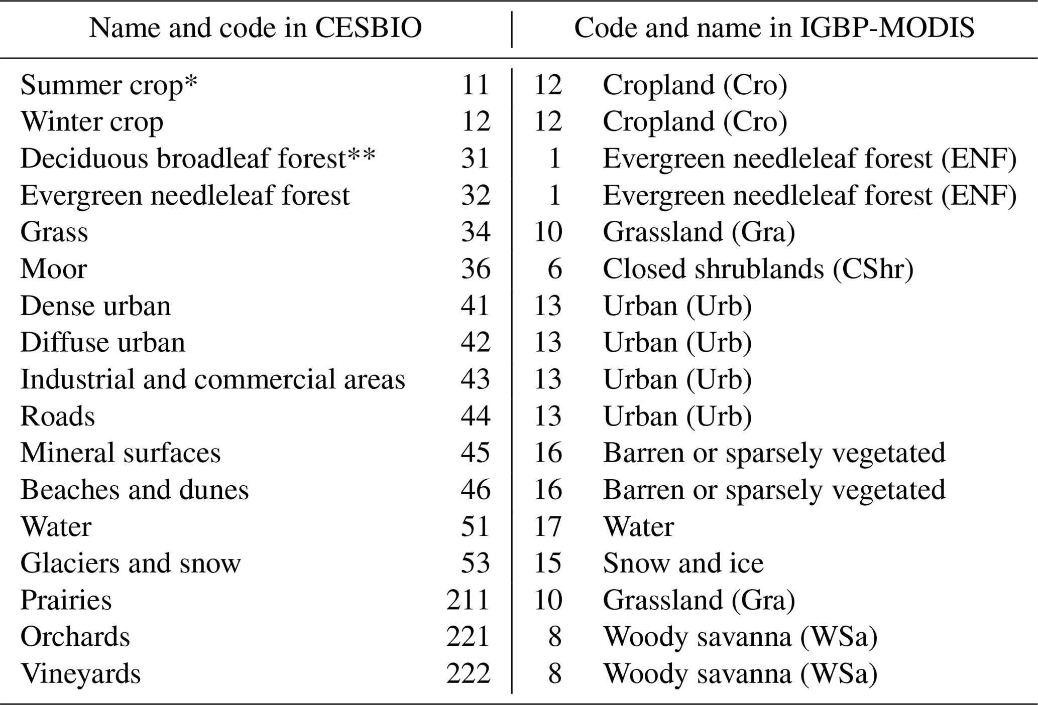
B1 NEW-LC experiment

Two variables were modified in the geo_em_d04.nc file (the fourth-domain output from the geogrid.exe programme of the WRF preprocessing system – WPS). On the one hand, the LANDUSEF variable was modified, including the new percentages for each LC category in all the 1 km grid cells of the fourth domain. The same was done for the rest of the domains, but only in the area covered by the inner domain. On the other hand, the dominant LC category in each pixel was calculated based on the new information, which served to modify the LU_INDEX variable in the same files as before.

These files with the modified LANDUSEF and LU_INDEX variables were re-incorporated into the WPS system, and the rest of the preprocessing programmes were executed, i.e. ungrib.exe and metgrid.exe, obtaining the final met_em files used to run the model. Note how in order to use these modified files in the model simulations, the surface_input_source parameter in the WRF namelist.input file was set to 3.

B2 MOSAIC experiment

To activate the mosaic approach, some options should be included in the namelist.input file of WRF. In the case of Noah, the sf_surface_mosaic option should be set to 1. The mosaic_cat option indicates the maximum number of tiles to be used, which was set to 19, the maximum possible in our area. In the case of RUC, the mosaic_lu and mosaic_soil should be included and set to 1.

B3 FOREST experiment

The three parameters modified in the FOREST experiment were changed in the MPTABLE.TBL file of WRF. This file contains the vegetation parameters tabulated from the different LC categories for the two LC datasets available in WRF. Since our simulations used the IGBP-MODIS LC dataset, we changed these parameters in the corresponding section within the file. Specifically, we modified MP from its original value (6) to 9, BP from 0.002 to 0.01 $\mathrm{mol}{\mathrm{H}}_{\mathrm{2}}\mathrm{O}{\mathrm{m}}^{-\mathrm{2}}{\mathrm{s}}^{-\mathrm{1}}$, and V_cmax25 from 50 to 62.5 $\mathrm{\mu }\mathrm{mol}{\mathrm{m}}^{-\mathrm{2}}{\mathrm{s}}^{-\mathrm{1}}$ for the LC type 1 (ENF). This was done before running the WRF simulation with the Noah-MP LSM.