the Creative Commons Attribution 4.0 License.
the Creative Commons Attribution 4.0 License.
 | 10 Sep 2020
Earth System Model Evaluation Tool (ESMValTool) v2.0 – diagnostics for emergent constraints and future projections from Earth system models in CMIP
Veronika Eyring
Omar Bellprat
Lisa Bock
Bettina K. Gier
Alasdair Hunter
Ruth Lorenz
Núria Pérez-Zanón
Mattia Righi
Manuel Schlund
Daniel Senftleben
Katja Weigel
Sabrina Zechlau
The Earth System Model Evaluation Tool (ESMValTool), a community diagnostics and performance metrics tool for evaluation and analysis of Earth system models (ESMs), is designed to facilitate a more comprehensive and rapid comparison of single or multiple models participating in the Coupled Model Intercomparison Project (CMIP). The ESM results can be compared against observations or reanalysis data as well as against other models including predecessor versions of the same model. The updated and extended version (v2.0) of the ESMValTool includes several new analysis scripts such as large-scale diagnostics for evaluation of ESMs as well as diagnostics for extreme events, regional model and impact evaluation. In this paper, the newly implemented climate metrics such as effective climate sensitivity (ECS) and transient climate response (TCR) as well as emergent constraints for various climate-relevant feedbacks and diagnostics for future projections from ESMs are described and illustrated with examples using results from the well-established model ensemble CMIP5. The emergent constraints implemented include constraints on ECS, snow-albedo effect, climate–carbon cycle feedback, hydrologic cycle intensification, future Indian summer monsoon precipitation and year of disappearance of summer Arctic sea ice. The diagnostics included in ESMValTool v2.0 to analyze future climate projections from ESMs further include analysis scripts to reproduce selected figures of chapter 12 of the Intergovernmental Panel on Climate Change's (IPCC) Fifth Assessment Report (AR5) and various multi-model statistics.


Climate models are important tools not only to improve our understanding of the key processes in present-day climate but also to project future climate change under different plausible scenarios. Climate models have been continuously improved and extended over the last decades from relatively simple atmosphere-only models to the complex state-of-the-art Earth system models (ESMs) participating in the latest (sixth) phase of the Coupled Model Intercomparison Project (CMIP6; Eyring et al., 2016a). The increasing complexity of the models is needed to represent key feedbacks that affect climate change but is also likely to increase the spread of climate projections across the multi-model ensemble (Eyring et al., 2019). This poses a challenge for evaluation and analysis of the model results that requires efficient tools able to handle the increasing number of variables, processes and also the increasing data volume.
The Earth System Model Evaluation Tool (ESMValTool), released in a first version in 2016 (Eyring et al., 2016b), has been developed with the aim of taking model evaluation to the next level by facilitating analysis of many different ESM components, providing well-documented source code and scientific background of implemented diagnostics and metrics and allowing for traceability and reproducibility of results (provenance). This has been made possible by a lively and growing development community continuously improving the tool supported by multiple national and European projects. Version 2.0 (v2.0) of the ESMValTool has been developed as a large community effort to specifically target the increased data volume of CMIP6 and the related challenges posed by analysis and evaluation of output from multiple high-resolution and complex ESMs.
For this, the core functionalities have been completely rewritten in order to take advantage of state-of-the-art computational libraries and methods to allow for faster, more efficient and user-friendly data processing (Righi et al., 2020). Besides many technical improvements, ESMValTool v2.0 includes new large-scale diagnostics for evaluation of Earth system models (Eyring et al., 2020) and diagnostics for extreme events, regional model and impact evaluation and analysis of ESM results (Weigel et al., 2020). As part of a series of four articles describing the new features and diagnostics of the Earth System Model Evaluation Tool v2.0, this paper focuses on the newly included diagnostics for emergent constraints and for analysis of future projections from ESMs as well as multi-model products (Sect. 3.1) and the two new climate metrics: effective climate sensitivity (ECS) and transient climate response (TCR) (Sect. 3.2).
An emergent constraint is a relationship across an ensemble of models between some aspect of the Earth system sensitivity and an observable trend or variation in the current climate, which offers the possibility to reduce uncertainties in climate projections. Furthermore, emergent constraints can help guide model development onto processes crucial to the magnitude and spread of future climate change projections and to point out future observational priorities (Eyring et al., 2019). Emergent constraints implemented in ESMValTool v2.0 (Sect. 3.3) include seven different approaches to constrain ECS as well as constraints for the hydrological cycle intensification, snow-albedo effect, year of disappearance of summer Arctic sea ice, future Indian summer monsoon precipitation and climate–carbon cycle feedback.
For the analysis of ESM projections, ESMValTool v2.0 now includes diagnostics to reproduce selected figures from chapter 12 (Long-term Climate Change: Projections, Commitments and Irreversibility) of the IPCC AR5 (Collins et al., 2013). These include figures showing the change in a variable between historical and future periods, e.g., maps (2-D variables), zonal means (3-D variables), time series showing the change in certain variables from historical to future periods for multiple scenarios and maps visualizing change in variables normalized by global mean temperature change (pattern scaling) and the possibility to show statistical significance of changes when compared to natural variability and the degree of agreement between the models using the stippling and hatching methods as in Collins et al. (2013). Furthermore, diagnostics tailored to analyze projections of sea ice such as calculation of the year of disappearance (sea ice extent below 1 million km2) from a multi-model ensemble and to constrain the future austral jet position have been added. A newly implemented “toy model” can be used to generate synthetic members of a single dataset. When providing an estimate for the standard error of observations, e.g., from differences between different observational datasets, this toy model can be used to investigate and take into account the effect of observational uncertainty in model evaluation (Sect. 3.4). A summary is given in Sect. 4. The aim of this paper is to document and illustrate how these newly added ESMValTool “recipes”, i.e., configuration files defining input, preprocessing, diagnostics and run-time options of the ESMValTool, can be used for model evaluation and analysis.
Table 1Overview of recipes for emergent constraints and future projections implemented in ESMValTool (v2.0) along with the section where they are described, a brief description, the required CMIP5 variables, the diagnostic scripts included and the observational datasets used in the examples. All diagnostics expect time series of monthly mean data as input. For further technical details, we refer to the GitHub repository.
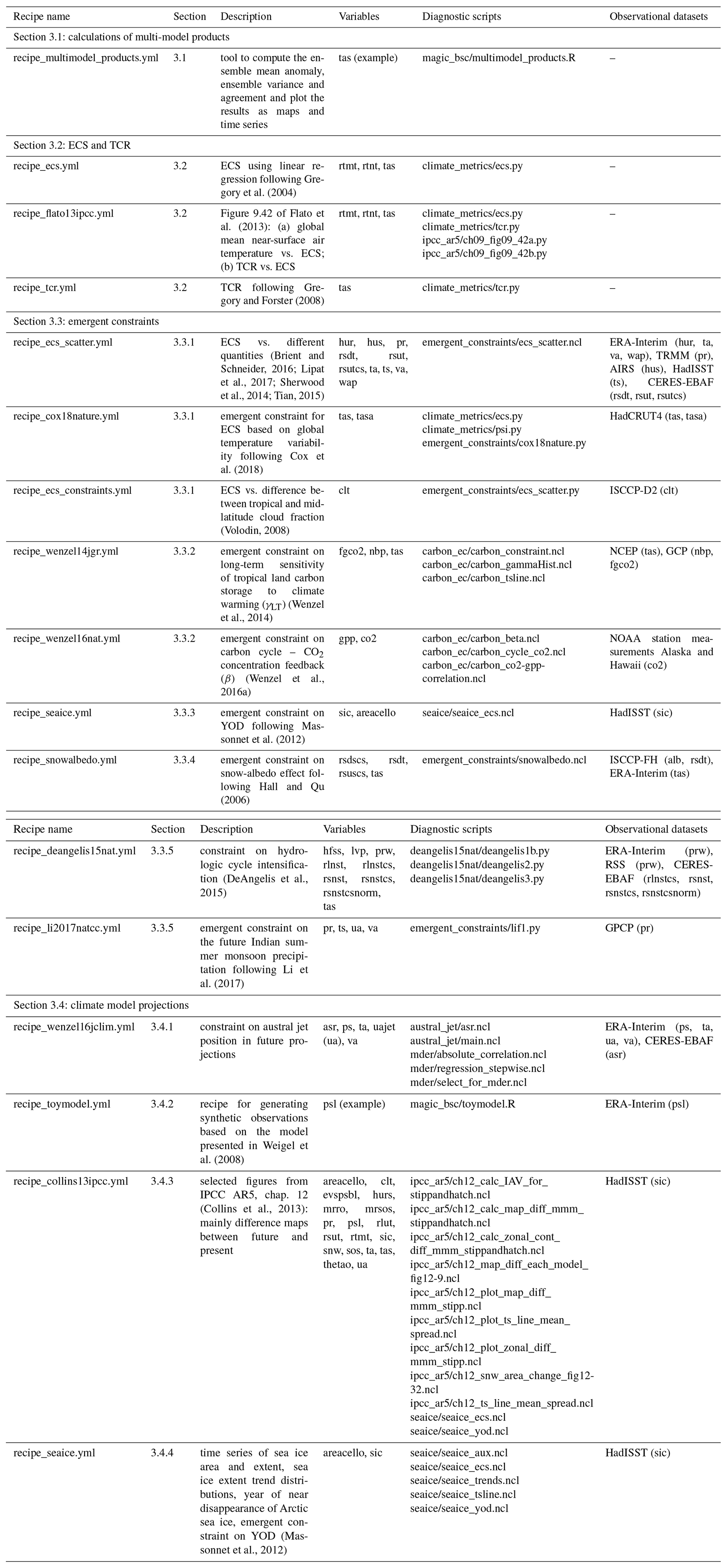
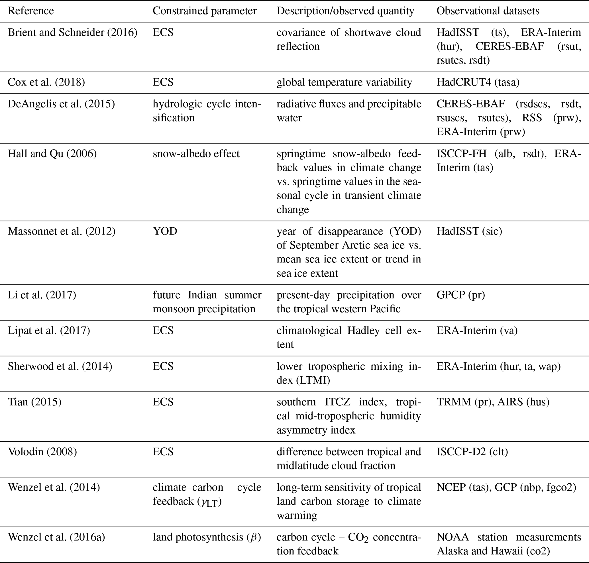
Table 2Emergent constraints implemented in ESMValTool v2.0 and observational datasets used.
The open-source release of ESMValTool (v2.0) that accompanies this paper is intended to work with CMIP5 and CMIP6 model output (and partly also with CMIP3 if the required output has been generated), but the tool is compatible with any arbitrary model output, provided that it is in CF-compliant (CF: Climate and Forecast; http://cfconventions.org/, last access: 18 June 2020) NetCDF format and that the variables and metadata are following the CMOR (Climate Model Output Rewriter; https://pcmdi.github.io/cmor-site/media/pdf/cmor_users_guide.pdf, last access: 18 June 2020) tables and definitions (e.g., https://github.com/PCMDI/cmip6-cmor-tables/tree/master/Tables, last access: 7 November 2019, for CMIP6). These tables read in by the ESMValTool contain the definition of all variables, together with their metadata such as units and standard and long names. Observations used in the evaluation are detailed in the various sections of the paper (see also Sect. 6) and summarized in Tables 1 and 2 but should also be seen as examples as they can be easily replaced by other observational datasets provided they follow the CMOR convention. For selected observational datasets, CMORizing scripts are provided with the ESMValTool that contain detailed downloading and processing instructions to convert the datasets into a CMOR-like format that can be processed by the ESMValTool. These reformat scripts serve as examples for writing similar scripts for other observational datasets that do not follow the CMOR standard. Such other datasets that are not available via the obs4mips (https://esgf-node.llnl.gov/projects/obs4mips/, last access: 26 February 2020) or ana4mips (https://esgf.nccs.nasa.gov/projects/ana4mips/, last access: 30 June 2019) projects and for which no CMORizing scripts are provided can be used with the ESMValTool in two ways. The first is to write a new CMORizing script using an available one as a template to generate a local copy of CMORized data that can readily be used with the ESMValTool. This typically involves saving only one variable per file and adding metadata such as coordinates (e.g., longitude, latitude, pressure level, time) and attributes (e.g., variable standard and long names, units, dimensions) according to the CMOR standard to the dataset(s). The second way is to implement specific “fixes” for this dataset in which case the CMORizing is performed “on the fly” during the execution of an ESMValTool recipe. For details on both methods, we refer to the ESMValTool user guide available at https://docs.esmvaltool.org/en/latest/input.html#observations (last access: 18 June 2020).
In this section, all diagnostics and metrics newly added to ESMValTool v2.0 for analysis of future projections from ESMs as well as the emergent constraints implemented are described and illustrated with examples using results from the CMIP5 model ensemble (Taylor et al., 2012). The ESMValTool workflow is controlled by configuration files called “recipes”, which define all input datasets, preprocessing steps and diagnostics to run (for details we refer to Righi et al., 2020). An overview of all recipes described in this paper including a short description, the variables processed, the names of the diagnostic scripts and observations is given in Table 1.
All diagnostics output one or more NetCDF file(s) containing the results of the analysis that are then visualized in the figure(s) created. The file format of the figures can be defined in the user configuration file and includes common formats such as *.png, *.pdf, *.ps and *.eps. For more details on the technical infrastructure of the tool including accepted data formats, data reference syntax (DRS) used for directory and file name conventions, available preprocessor functions, etc., we refer again to Righi et al. (2020). Further information can be found in the ESMValTool user guide, which documents all technical aspects of the tool as well as all available diagnostics; see https://docs.esmvaltool.org/ (last access: 1 September 2020).
3.1 Calculations of multi-model products
Multi-model means are commonly used to project climate change (IPCC, 2013, 2007) and are thus a useful quantity to calculate in support of diagnostics included in the ESMValTool.

Figure 1Multi-model mean of projected future June near-surface air temperature anomalies (2006–2099) compared with the period of 1961–1990 (colors). Crosses indicate that the 80 % of models agree with the sign of the multi-model mean anomaly. The models used in this example are BCC-CSM1-1, MPI-ESM-MR and MIROC5 (r1i1p1 ensembles) for the RCP2.6 scenario. All models have been regridded to the BCC-CSM1-1 grid using a linear interpolation scheme. See Sect. 3.1 for details on recipe_multimodel_products.yml.
The recipe recipe_multimodel_products.yml computes the multi-model ensemble mean for a set of models selected by the user for individual variables and different temporal resolutions (annual, seasonal, monthly). For this, all data are regridded to the same horizontal grid. In the example shown in Fig. 1, all models are regridded to the grid of BCC-CSM1-1 using a linear interpolation scheme. This task is done by the ESMValTool's preprocessor and defined in the recipe depending on the application and user requirements. The user-definable configuration options include definition of the target grid (e.g., 2.5∘ × 2.5∘) and regridding scheme (e.g., linear, nearest, area weighted). Regridding/interpolation of the input data in time is currently not supported. For further details, we refer to the ESMValTool user guide (https://docs.esmvaltool.org/, last access: 1 September 2020). After selecting the region (rectangular region defined by the lowermost and uppermost longitudes and latitudes), the mean for the selected reference period is subtracted from the time series in order to obtain the anomalies for the desired period. In addition, the recipe computes the percentage of models agreeing on the sign of this anomaly, thus providing some information on the robustness of the climate change signal.
The output of the recipe consists of a contour map showing the time average of the multi-model mean anomalies and stippling to indicate locations where the percentage of models agreeing on the sign of the multi-model mean anomaly exceeds a threshold selected by the user (Fig. 1). The example in Fig. 1 shows a warming over the continents in the range of 1–2 K which is more pronounced than the warming over the ocean which is mostly in the range of 0.5–1.5 K in this scenario. The example also shows that the models largely agree on the sign of the temperature change with the most prominent exceptions found in parts of the Southern Ocean, Greenland and the North Atlantic. Furthermore, a time series of the area-weighted mean anomalies is plotted. For the plots, the user can select the length of the running window for temporal smoothing and choose to display either the ensemble mean with a light shading to represent the spread of the ensemble or each individual model separately (Fig. 2). The example in Fig. 2 shows an increase in global average June temperatures up to about 2060 when temperatures start to level off. By 2100, the four CMIP5 example models (MPI-ESM-MR, CNRM-CM5, BCC-CSM1-1 and IPSL-CM5A-LR) show a spread in temperature increase for the RCP2.6 scenario ranging from 0.7 to about 1.8 K.
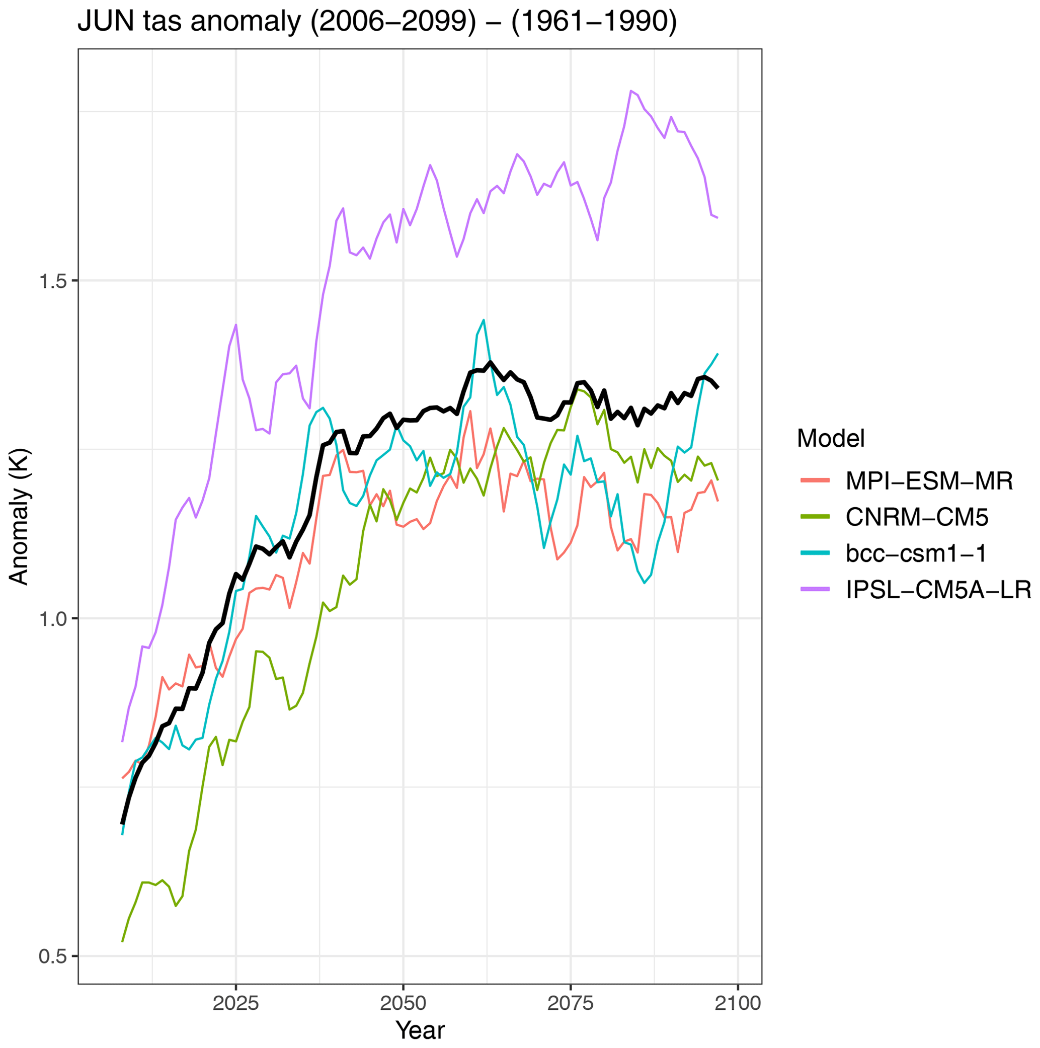
Figure 2Time series of global average near-surface air temperature anomalies in June for the period of 2006–2099 (RCP2.6 scenario) compared to the reference period of 1961–1990. The individual models are shown as colored lines; the multi-model mean is shown in black. See Sect. 3.1 for details on recipe_multimodel_products.yml.
3.2 ECS and TCR
The ECS is an important metric to assess the future warming of the climate system. It is defined as the change in global mean near-surface air temperature as a result of a doubling of the atmospheric CO2 concentration compared to pre-industrial conditions after the climate system has reached a new equilibrium (Gregory et al., 2004). Climate models of the CMIP5 model ensemble simulated an ECS ranging between 2.1 and 4.7 K (Flato et al., 2013). Using all available evidence of that time, IPCC AR5 assessed a “likely” range of ECS between 1.5 and 4.5 K in 2013 (IPCC, 2013). recipe_ecs.yml uses a regression method proposed by Gregory et al. (2004) to calculate ECS. Using the total radiative forcing F caused by the doubling of atmospheric CO2 concentration and the climate feedback parameter λ, ECS is defined as . Both of these variables can be assessed by linear regression of the equation for radiative balance , where N is the net radiation flux at the top of the atmosphere (TOA) and ΔT the global mean near-surface air temperature change. N and ΔT are both given as global and annual mean differences between the abrupt quadrupled CO2 simulation and the linear regression of the pre-industrial control run. Figure 3 illustrates this regression for the CMIP5 multi-model mean. Moreover, it shows that the assumption of a linear climate feedback parameter is only an approximation. Using only the first 20 years (last 130 years) instead of all 150 years of the abrupt quadrupled CO2 simulations results in a stronger (weaker) feedback, which again leads to a lower (higher) ECS. This demonstrates the different response of the climate system at different timescales, i.e., non-linear feedback processes. This diagnostic requires the input variables near-surface air temperature (tas), TOA incoming shortwave radiation (rsdt), TOA outgoing shortwave radiation (rsut) and TOA outgoing longwave radiation (rlut) from abrupt4xCO2 (quadrupling of CO2 compared to pre-industrial conditions) and piControl (pre-industrial control) simulations.
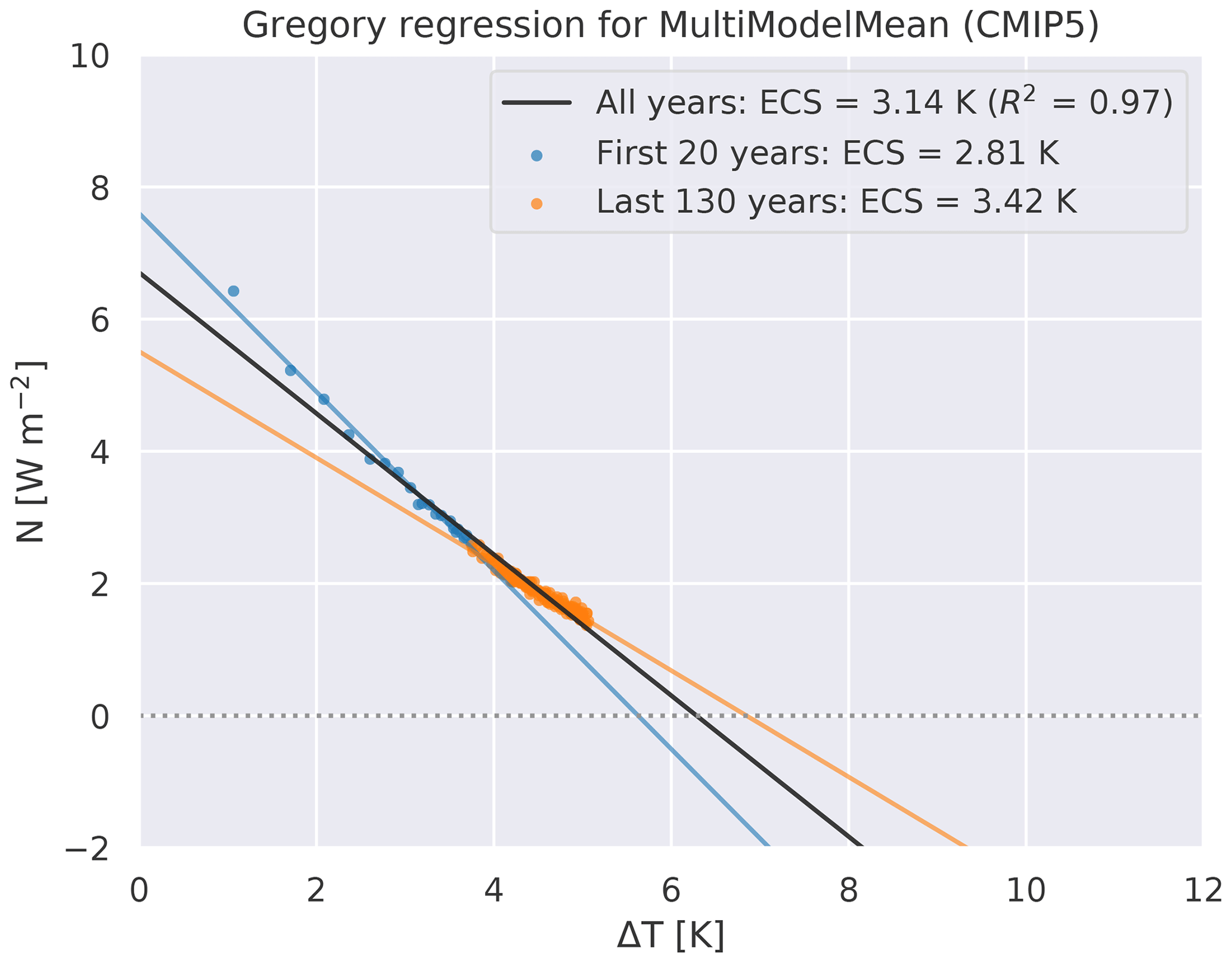
Figure 3Gregory plot to approximate the ECS (Gregory et al., 2004). Shown is the relationship between the differences in global and annual mean top-of-the-atmosphere net downward radiative flux N (W m−2) and global and annual mean near-surface air temperature anomalies ΔT (K) for the CMIP5 multi-model mean. Anomalies are calculated as difference between the abrupt4xCO2 experiment (quadrupling of CO2) and the pre-industrial control run (piControl). The blue dots show the first 20 years of the simulation; the orange dots show the last 130 years. A linear regression using only the first 20 years (blue line) instead of all 150 years (black line) results in a stronger feedback (and thus lower ECS). Using the last 130 years only (orange line) results in a weaker feedback (i.e., higher ECS). See Sect. 3.2 for details on recipe_ecs.yml.
Figure 9.42a of Flato et al. (2013) shows the globally averaged mean near-surface air temperature (GMSAT) for the historical period of 1961–1990 plotted vs. ECS of several CMIP5 models. The latter quantity can be calculated by a regression method based on Gregory et al. (2004) as outlined above. A similar figure produced with recipe_flato13ipcc.yml implemented in ESMValTool v2.0 shows that there are no distinctive correlations between the historical surface temperatures and the ECS, which suggests that the ECS is not very sensitive to errors in the current climate in contrast to other sources of uncertainty (Fig. 4).
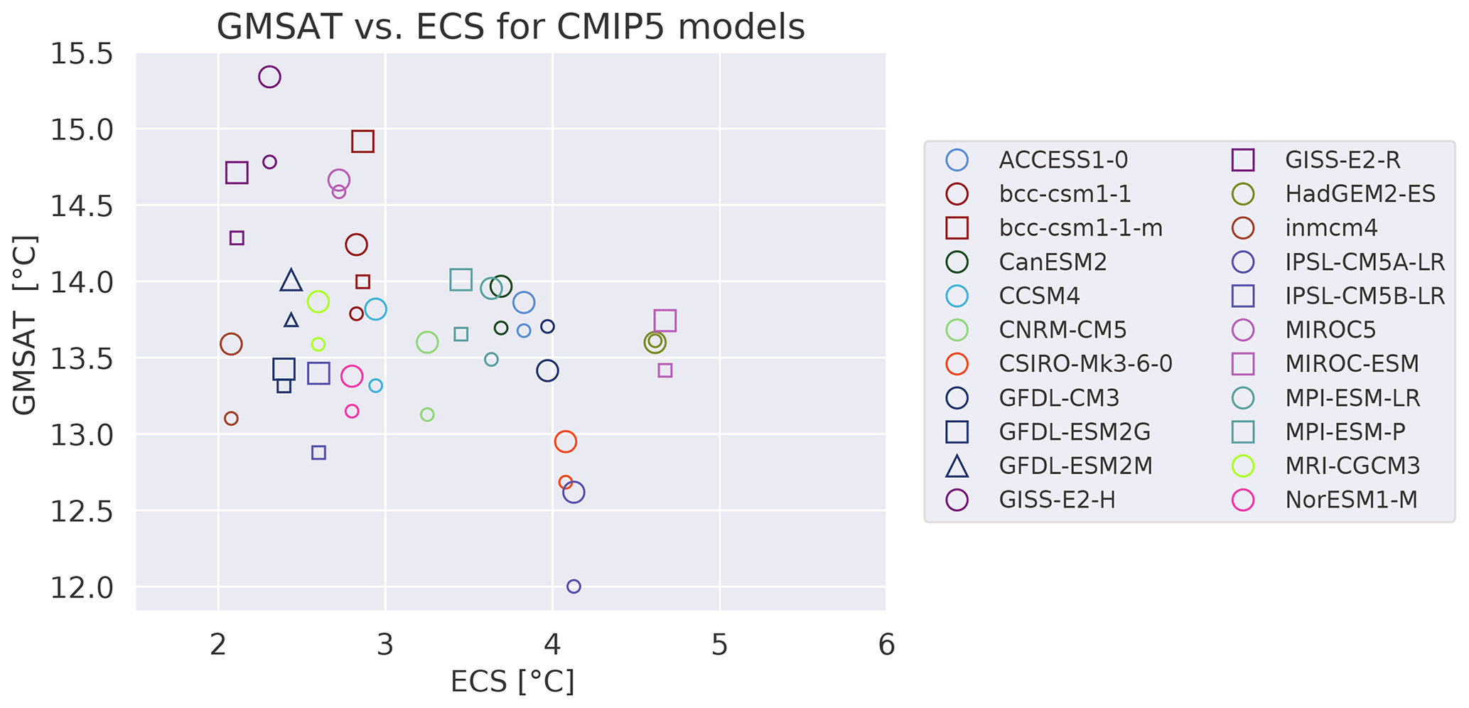
Figure 4Globally averaged near-surface air temperature (GMSAT) of the historical period of 1961–1990 vs. the ECS for several CMIP5 models. Similar to Fig. 9.42a of Flato et al. (2013) and produced with recipe_flato13ipcc.yml; see details in Sect. 3.2.
The TCR is defined as the global and annual mean near-surface air temperature anomaly in the 1pctCO2 simulation (1 % increase in CO2 per year) for a 20-year period centered at the time of CO2 doubling, i.e., using the years 61 to 80 after the start of the simulation. The temperature anomalies are calculated by subtracting a linear fit to the piControl run for all 140 years from the 1pctCO2 experiment prior to the TCR calculation (Gregory and Forster, 2008). Figure 5 shows (a) a time series of the 1pctCO2 near-surface temperature anomalies from MIROC-ESM used to obtain TCR and (b) TCR values for different CMIP5 models calculated with recipe_tcr.yml.
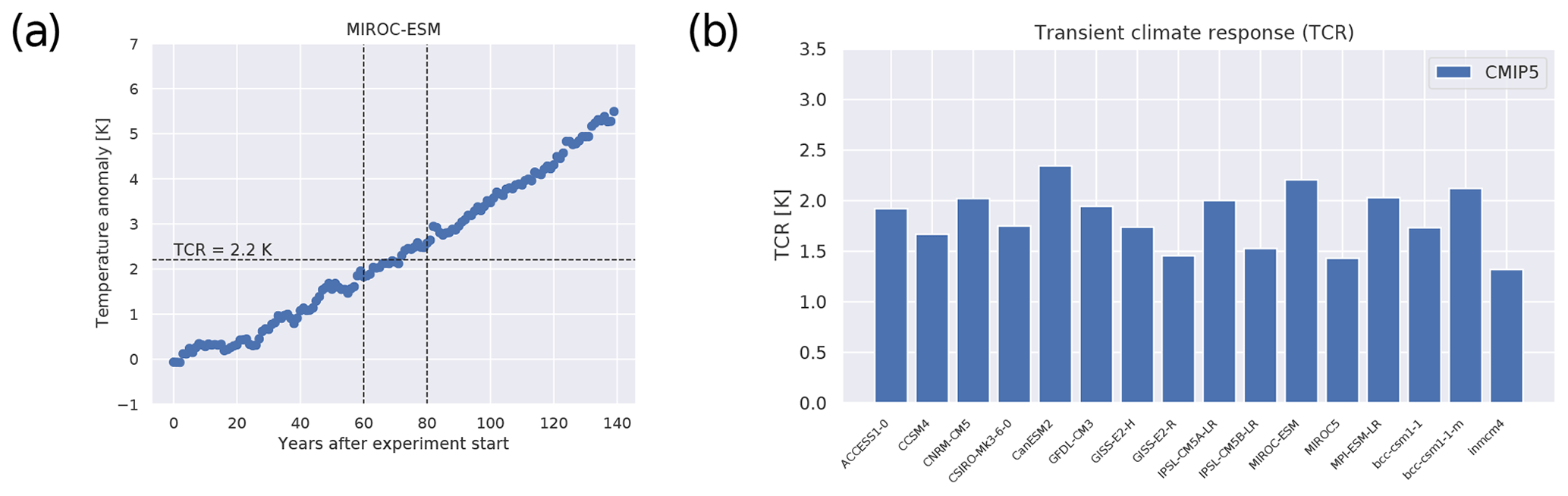
Figure 5(a) Time series of temperature anomalies from MIROC-ESM experiment 1pctCO2 (1 % increase in CO2 per year) compared to the piControl simulation. (b) Transient climate response (in K) for CMIP5 models calculated with the method by Gregory and Forster (2008). For details on recipe_tcr.yml, see Sect. 3.2.
3.3 Emergent constraints
An emergent constraint utilizes an ensemble of ESMs together with observational data to constrain a simulated future Earth system feedback. A prerequisite for an emergent constraint is a robust relationship between, for example, changes occurring on seasonal or interannual timescales and changes found in ESM simulations of anthropogenically forced climate change (Eyring et al., 2019). If such a relationship can be explained by a plausible physical mechanism, an observational constraint of multi-model projections of quantities that cannot be observed directly might be possible. Such a non-observable quantity is, for instance, ECS. The technique of emergent constraints offers the possibility to reduce uncertainties in climate projections and can help guide model development by highlighting processes that are crucial to explaining the magnitude and spread of the modeled future climate change. Emergent constraints can also help point out the need for more and/or more reliable observations.
We would like to note that a limitation of the emergent constraints as currently implemented into the ESMValTool is that model interdependency, as in the original studies, is not explicitly taken into account. As some modeling groups share model components or code, the models are not all independent. Duplicated code, as well as identical forcing and validation data in multiple models, is expected to lead to an overestimation of the sample size of a model ensemble and may result in spurious correlations (Sanderson et al., 2015). As a possible approach, future implementations of these emergent constraints could, for example, apply a model weighting based on a model's interdependence (e.g., Knutti et al., 2017) or simply reduce the ensemble size by taking into account only models that are above a given yet-to-be-defined interdependence score.
Table 2 summarizes the emergent constraints that have been implemented in ESMValTool (v2.0) including the observational datasets used and are described in the following.
3.3.1 Emergent constraints on effective climate sensitivity
recipe_ecs_scatter.yml calculates five emergent constraints for ECS (see Table 2). These are briefly described in Sect. 3.3.1 (“Covariance of shortwave cloud reflection” to “Tropical mid-tropospheric humidity asymmetry index”). The ECS values from the models are pre-calculated with recipe_ecs.yml (see Sect. 3.2) or can be taken from literature. The diagnostic calculates ECS vs. selected constraining parameters, such as the climatological Hadley cell extent from models, and fits a linear regression line to the data. If available, the observational uncertainty of a given observational dataset can be estimated. For this, the standard error of the observations is subtracted or added from or to the means before calculating the observational value (estimated minimum or maximum, respectively). In addition to the scatter plots of ECS vs. constraining parameter calculated by the diagnostic, the diagnostic also outputs the 25 %/75 % confidence intervals of the regression (i.e., uncertainty of the fit) and the 25 %/75 % prediction intervals of the regression (i.e., measure for the quality of the linear fit). By definition, 50 % of all model data points are within the 25 %/75 % prediction interval of the regression line. Examples of the different scatter plots that can be created by recipe_ecs_scatter.yml are shown in Fig. 6. It should be noted that because a different set of CMIP5 models might be used in the figures compared to the originally published emergent constraints, the figures could show some deviations to the ones published in literature. While the emergent constraints shown in Fig. 6a, c, d, e suggest ECS values in the upper range of the values given in IPCC AR5 (IPCC, 2007, 1.5 to 4.5 K), the emergent constraint shown in Fig. 6b suggests an ECS value in the lower range of the IPCC AR5 values.
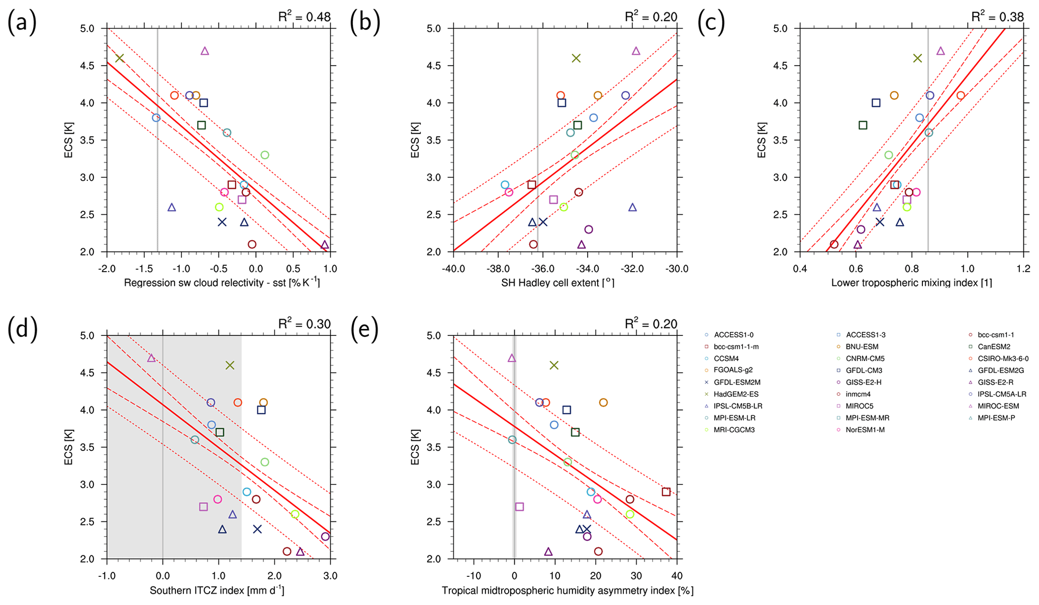
Figure 6Scatter plots of ECS vs. (a) covariance of shortwave cloud reflection (Brient and Schneider, 2016), (b) Southern Hemisphere (SH) climatological Hadley cell extent (Lipat et al., 2017), (c) lower tropospheric mixing index (LTMI) (Sherwood et al., 2014), (d) southern Intertropical Convergence Zone (ITCZ) index (Tian, 2015) and (e) tropical mid-tropospheric humidity asymmetry index (Tian, 2015) for CMIP5 models (symbols). The vertical gray lines represent the observations; the shaded areas in light gray represent observational uncertainties (if available). The solid red lines represent the regression lines, the dashed red lines the 25 %/75 % confidence intervals of the regression and the dotted red lines the 25 %/75 % prediction intervals of the regression. Similar to (a) Fig. 6 of Brient and Schneider (2016), (b) Fig. 4 of Lipat et al. (2017), (c) Fig. 5c of Sherwood et al. (2014), (d) Fig. 2 of Tian (2015) and (e) Fig. 4c of Tian (2015). For details on recipe_ecs_scatter.yml, see Sect. 3.3.1.
In addition to these five emergent constraints, recipe_cox18nature.yml implements an emergent constraint for ECS based on global temperature variability (Sect. 3.3.1, “Global temperature variability”), recipe_ecs_constraints.yml an emergent constraint based on the difference between tropical and midlatitude cloud fraction (Sect. 3.3.1, “Difference between tropical and midlatitude cloud fraction”).
Covariance of shortwave cloud reflection
This emergent constraint uses the models' correlation of tropical low-level cloud (TLC) reflection with the underlying SST to constrain ECS (Brient and Schneider, 2016). The definition and calculation of the individual terms follows Brient and Schneider (2016): TLC regions are defined as the 25 % ocean areas between 30∘ S and 30∘ N with the lowest 500 hPa relative humidity. TLC reflection is calculated as the ratio of top-of-the-atmosphere shortwave cloud radiative forcing and insolation, both averaged over the TLC region. This is then used to calculate the regression coefficients of deseasonalized variations of TLC shortwave reflection and sea surface temperature in % per K used as an emergent constraint. In the example shown in Fig. 6a, data from the CMIP5 historical simulations between 1980 and 2005 are used for the models, observational/reanalysis data used in Fig. 6 are ERA-Interim (Dee et al., 2011) for relative humidity, HadISST (Rayner et al., 2003) for sea surface temperatures and CERES-EBAF (Ed2.7) (Loeb et al., 2012) for top-of-the-atmosphere radiative fluxes.
Climatological Hadley cell extent
Lipat et al. (2017) found that the climatological mean Hadley cell (HC) edge latitude from CMIP5 models correlates with ECS. The HC edge latitude is calculated from first two grid cells from the Equator going south where the zonal average 500 hPa mass stream function changes sign from negative to positive (downward branch of the HC). The mass stream function is calculated from climatological December–January–February (DJF) means of the meridional wind fields. The correlation of the climatological HC extent with ECS found in CMIP5 models is explained by observations that show a correlation of variability in midlatitude clouds and cloud radiative effects with poleward HC expansion (Lipat et al., 2017). For the example shown in Fig. 6b, CMIP5 data from historical simulations and ERA-Interim (Dee et al., 2011) are used as a reference dataset for the years 1980–2005.
Lower tropospheric mixing index
Following Sherwood et al. (2014), the lower tropospheric mixing index (LTMI) can be used to constrain ECS and is calculated as the sum of small-scale mixing S and the large-scale component of mixing D. S is calculated from relative humidity (RH) and temperature (T) differences between 700 and 850 hPa and averaged over a tropical region between 30∘ S and 30∘ N defined by the upper quartile of the annual mean 500 hPa ascent rate within ascending regions: . The large-scale component of mixing is the ratio of shallow to deep overturning: with ω1 the average of the vertical velocity at 850 and 700 hPa, ω2 the average of the vertical velocity at 600, 500 and 400 hPa, H the step function and 〈…〉 the average over the tropical ocean region 30∘ S–30∘ N, 160∘ W–30∘ E. The lower tropospheric mixing index is calculated as . Sherwood et al. (2014) explain the correlation between LTMI and ECS in CMIP3 and CMIP5 models by convective mixing between the lower and middle tropical troposphere dehydrating low-level cloud layers at an increasing rate as climate warms. They argue that this rate of increase depends on initial mixing strength, which links the mixing to clouds feedbacks and thus ECS. Figure 6c shows an example of this emergent constraint applied to CMIP5 historical simulations using ERA-Interim data (Dee et al., 2011) as reference data. All datasets in this example cover the time period of 1980–2005.
Southern ITCZ index
The southern Intertropical Convergence Zone (ITCZ) index (Bellucci et al., 2010; Hirota et al., 2011) is defined as the climatological annual mean precipitation bias averaged over the south-eastern Pacific (30∘ S–0∘, 150–100∘ W) given in mm d−1. The southern ITCZ index is used to quantify the double-ITCZ bias in CMIP3 and CMIP5 models and has been found to correlate with ECS (Tian, 2015). In the example shown in Fig. 6d, the ITCZ index has been calculated from CMIP5 historical model simulations averaged over the years 1980–2005. Tropical Rainfall Measuring Mission (TRMM) (Huffman et al., 2007) satellite data (v7) averaged over the years 1998–2013 have been used as observational reference.
Tropical mid-tropospheric humidity asymmetry index
The strong link found in CMIP3 and CMIP5 models between the double-ITCZ bias and simulated moisture, precipitation, clouds and large-scale circulation allows the double-ITCZ bias and thus ECS to also be related to mid-tropospheric humidity over the tropical Pacific (Tian, 2015). As shown by Tian (2015), spatial patterns of mid-tropospheric humidity and precipitation are similar as both are related to the ITCZ. This allows defining a tropical mid-tropospheric humidity asymmetry index to quantify the double-ITCZ bias in models and consequently constrain ECS. This index is defined as relative bias in simulated annual mean 500 hPa specific humidity compared with observations () averaged over the Southern Hemisphere (SH) tropical Pacific (30∘ S–0∘, 120∘ E–80∘ W) minus the bias averaged over the Northern Hemisphere (NH) tropical Pacific (20∘ N–0∘, 120∘ E–80∘ W) (Tian, 2015). The example for the tropical mid-tropospheric humidity asymmetry index shown in Fig. 6e is calculated from CMIP5 historical runs averaged over the years 1980–2005 and AIRS (v5) satellite data (Susskind et al., 2006) averaged over the years 2003–2010 as observational reference data.
Global temperature variability
Cox et al. (2018) propose an emergent constraint for the ECS using global temperature variability. The latter is defined by a metric ψ which can be calculated from the global temperature variance (in time) σT and the 1-year-lag autocorrelation of the global temperature α1T by
Using the simple “Hasselmann model” (Hasselmann, 1976), Cox et al. (2018) showed that ψ is linearly correlated with ECS in CMIP5 data. Since calculation of ψ only depends on the temporal evolution of the global surface temperature, there are many observational datasets available. In the original publication, data from HadCRUT4 (Morice et al., 2012) are used to construct the emergent relationship. In the ESMValTool, this is reproduced by recipe_cox18nature.yml, which only needs two variables: historical near-surface air temperature (tas) and ECS (see Sect. 3.2). The emergent relationship between ECS and ψ is shown in Fig. 7 including means and confidence intervals. The constrained range of ECS based on this plot is 2.2 to 3.4 K with a 66 % confidence interval, similar to Cox et al. (2018).
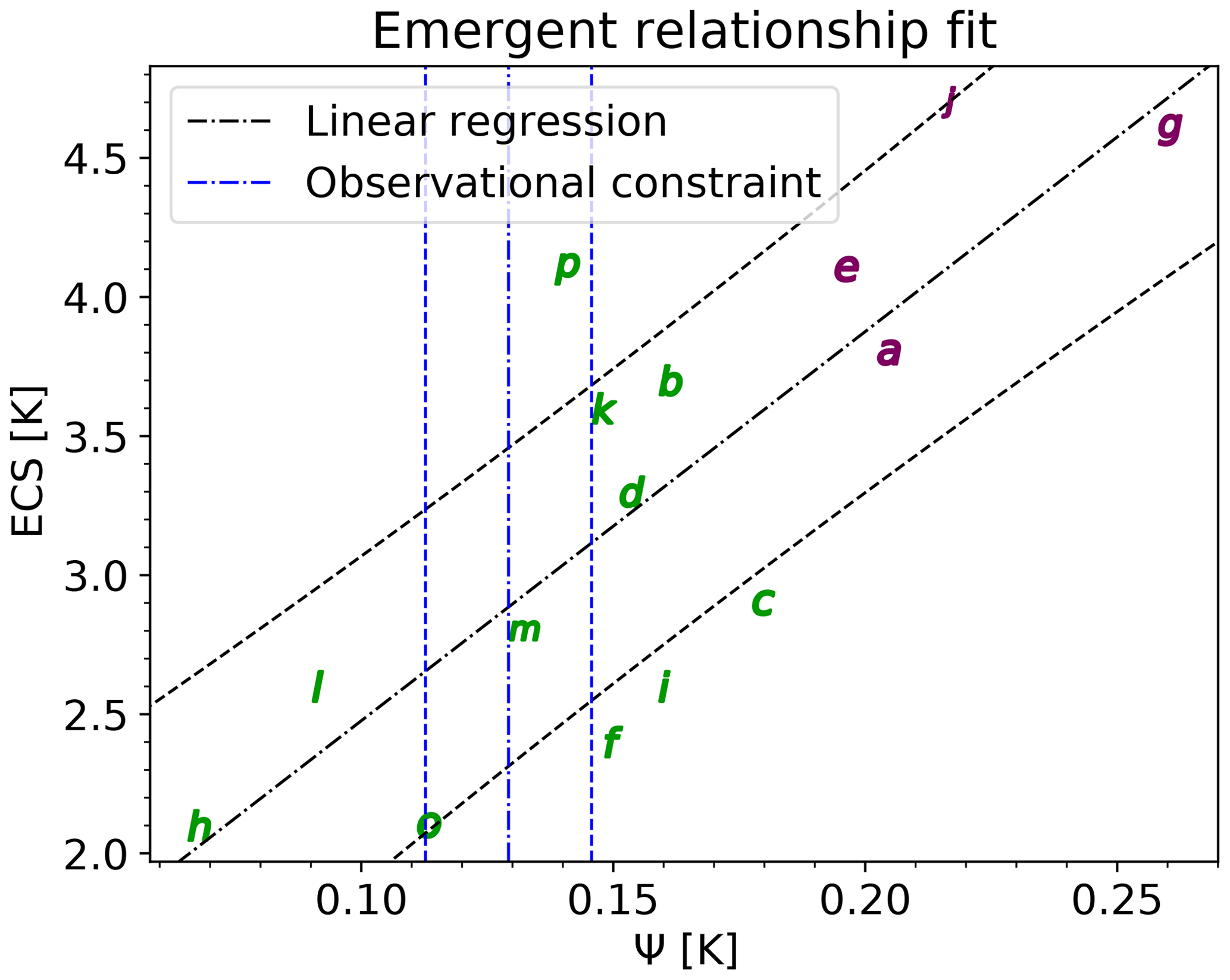
Figure 7Emergent constraint for ECS. Shown is the relationship between ECS and the temperature variability metric ψ proposed by Cox et al. (2018). Letters show individual CMIP5 models (for nomenclature details, see original publication) with lower-sensitivity models in green and higher-sensitivity models in purple. The black lines show the linear fit including the prediction error and the vertical blue lines indicate the observational mean and standard deviation given by the HadCRUT4 dataset. Similar to Fig. 2 of Cox et al. (2018) and produced with recipe_cox18nature.yml (see details in Sect. 3.3.1, “Global temperature variability”).
Difference between tropical and midlatitude cloud fraction
Volodin (2008) proposes an emergent constraint for ECS based on the distribution of clouds in global climate models. The study finds that models with high climate sensitivity show a higher total cloud cover over the southern midlatitudes and a lower total cloud cover over the tropics than the multi-model average. Thus, the difference in tropical total cloud cover (between 28∘ S and 28∘ N) and the SH midlatitude total cloud cover (between 56 and 36∘ S) is negatively correlated with ECS. The original publication uses the CMIP3 ensemble and the International Satellite Cloud Climatology Project (ISCCP)-D2 dataset (Rossow and Schiffer, 1991) as observational reference, but the relationship also holds when using CMIP5 models. In the ESMValTool, this emergent constraint for ECS can be produced with recipe_ecs_constraints.yml, which uses CMIP5 historical runs averaged between 1980 and 2000 (Fig. 8). The observed values are based on ISCCP-D2 data and are taken from Volodin (2008).
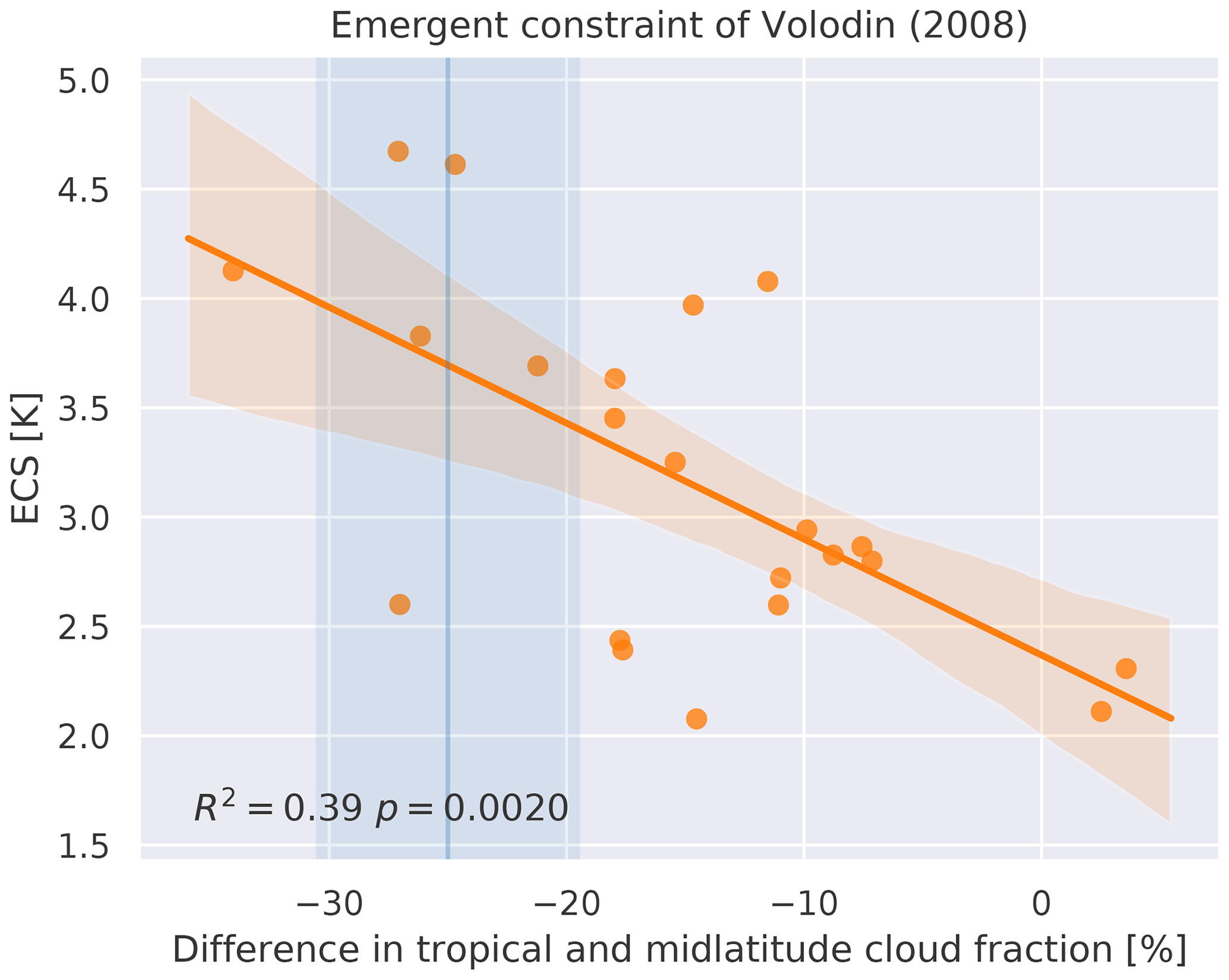
Figure 8ECS vs. difference in total cloud cover between the tropics (28∘ S–28∘ N) and southern midlatitudes (56–36∘ S) for CMIP5 models (orange dots). The orange line and shaded area show the linear regression line and its 95 % uncertainty range (estimated via bootstrapping). Together with the observational estimate (vertical blue line and shaded area), this can be used as an emergent constraint for ECS (Volodin, 2008). The observational range is based on ISCCP-D2 data (Rossow and Schiffer, 1991) and taken from Volodin (2008). Similar to Fig. 3a of Volodin (2008) and produced with recipe_ecs_constraints.yml (see details in Sect. 3.3.1, “Difference between tropical and midlatitude cloud fraction”).
3.3.2 Emergent constraints on the carbon cycle
Uncertainties in projections of future temperature using ESMs are high, in a large part due to uncertainties of emissions and feedbacks. Within the carbon cycle, feedbacks are usually split into the carbon cycle – climate feedback γ, which quantifies carbon to climate change, and the carbon cycle – CO2 concentration feedback β, which is the carbon sensitivity to atmospheric CO2 (Friedlingstein et al., 2006). γ is a positive feedback as climate warming reduces the efficiency of CO2 absorption by the land and ocean, leading to more of the emitted carbon staying in the atmosphere, which in turn leads to additional warming. In contrast, β is a negative feedback because of the so-called CO2 fertilization effect, where plants take up a higher amount of CO2 for photosynthesis with increasing atmospheric CO2 concentrations. Efforts have been made to reduce the uncertainties of these two carbon cycle feedback parameters.
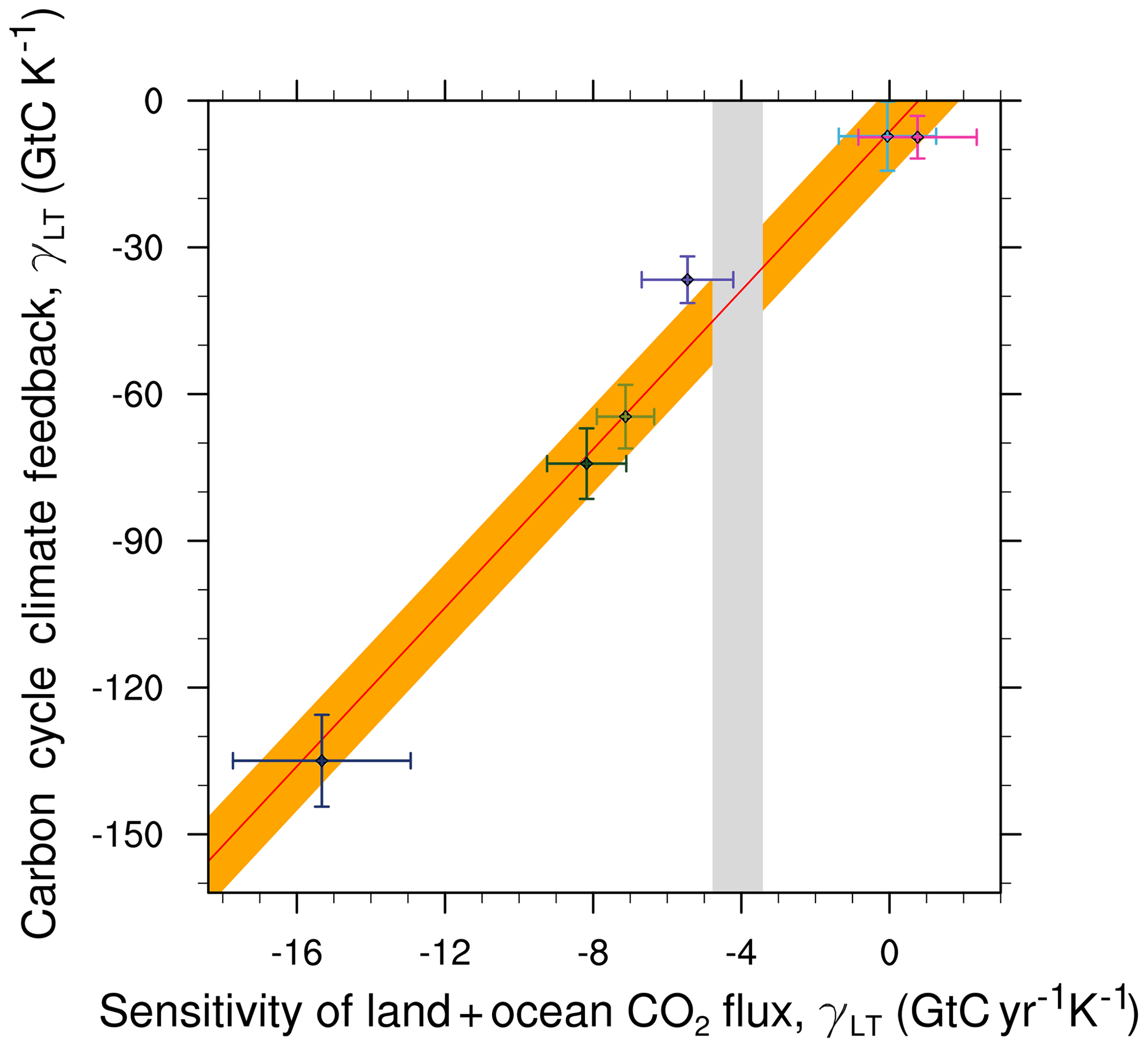
Figure 9Relationship between long-term sensitivity of tropical land carbon storage to climate warming (γLT) and short-term sensitivity of atmospheric CO2 to interannual temperature variability (γIAV) for CMIP5 models (markers with horizontal and vertical error bars) using the historical simulation. The red line shows the linear regression through the CMIP5 models; the vertical gray area shows the range of observed γIAV. Produced with recipe_wenzel14jgr.yml, similar to Fig. 5a of Wenzel et al. (2014) (for details, see Sect. 3.3.2).
Wenzel et al. (2014) employed the emergent constraint described by Cox et al. (2013) for the long-term sensitivity of tropical land carbon storage to climate warming (γLT) to the interannual sensitivity of atmospheric CO2 to interannual tropical temperature variability (γIAV) in CMIP5 models. The analysis from this paper can be reproduced using recipe_wenzel14jgr.yml with the emergent relationship being able to reduce the range of projected γLT (Fig. 9). Input variables include net primary productivity (nbp), surface temperature (tas), gas exchange flux of CO2 into the ocean (fgco2) from the experiment 1pctCO2, nbp, fgco2, tas from the emission-driven historical simulations (esmHistorical), as well as nbp from the esmFixClim1 (carbon cycle sees CO2 concentration increase but radiation does not) simulations. The different simulations are included in γIAV, which is estimated from both the 1pctCO2 experiment and the esmHistorical simulation, and then compared in the paper. The default observational datasets are NCEP reanalysis (Kalnay et al., 1996) for the surface temperature and the Global Carbon Project (GCP; Le Quere et al., 2015) for the carbon fluxes.
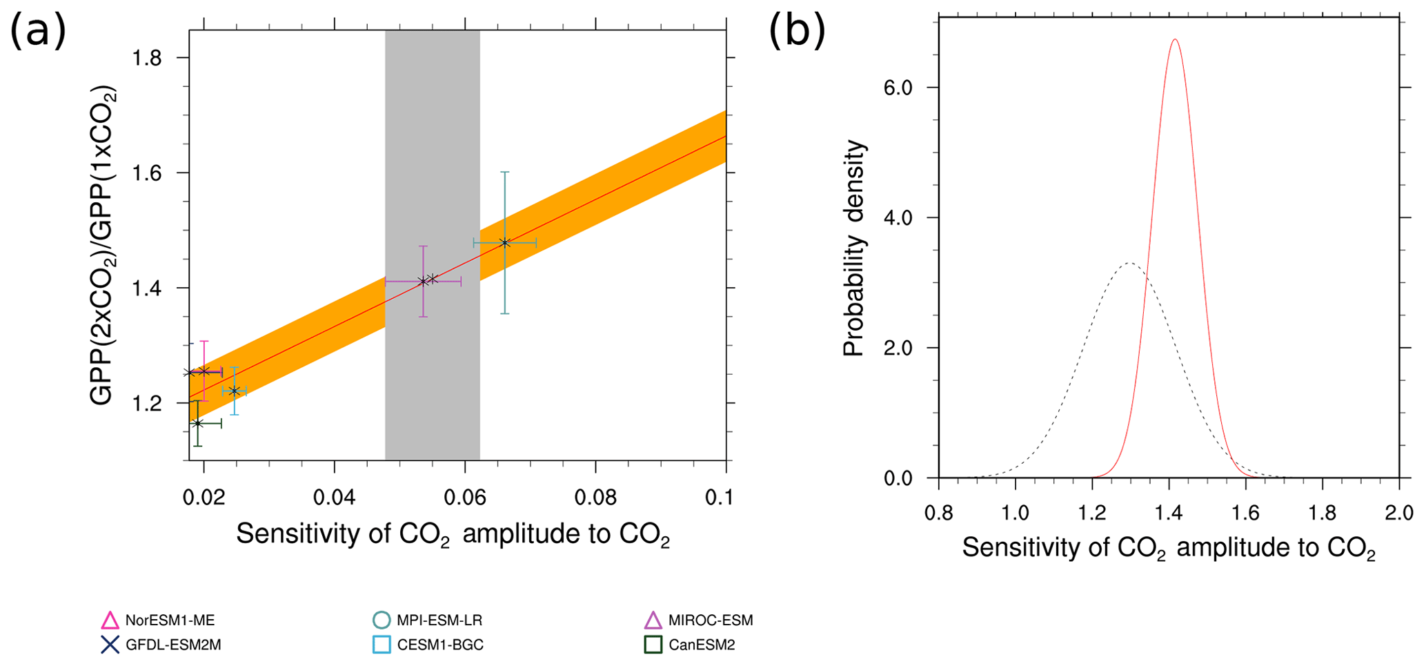
Figure 10(a) Correlations between the sensitivity of the CO2 amplitude to annual mean CO2 increases at Point Barrow, Alaska (abscissa), and the high-latitude (60–90∘ N) CO2 fertilization of GPP at twice the CO2. The gray shading shows the range of the observed sensitivity. The red line shows the linear best fit across the CMIP5 ensemble together with the prediction error (orange) and error bars show the standard deviation for each data point. (b) The probability density function for the unconstrained CO2 fertilization of GPP (black, dotted) and the conditional probability density function arising from the emergent constraint (red). Produced with recipe_wenzel16nat.yml, similar to Fig. 3 of Wenzel et al. (2016a) (for details, see Sect. 3.3.2).
Wenzel et al. (2016a) developed an emergent constraint for β on land in the extratropics and northern midlatitudes constraining the projected land photosynthesis with changes in the seasonal cycle of atmospheric CO2. The figures from this paper can be reproduced with recipe_wenzel16nat.yml, with Fig. 10 showing the emergent constraint reproduced with the ESMValTool. The unconstrained CO2 fertilization effect lies at 40±20 %, which can be narrowed down to 37±9 % in high latitudes and 32±9 % in the extratropics with this emergent constraint. Input variables from the models needed to run this recipe is gross primary productivity (GPP) in the esmFixClim1 simulations, as well as the atmospheric CO2 concentration (co2) from emission-driven historical simulations. Observations used are the atmospheric CO2 concentrations at Point Barrow (BRW; 71.3∘ N, 156.6∘ W), Alaska, and Cape Kumukahi, Hawaii (KMK; 19.5∘ N, 155.6∘ W) (NOAA, 2018).
3.3.3 Emergent constraints on the year of disappearance of September Arctic sea ice
This sea ice diagnostic produces scatter plots of (a) mean of and (b) trend in historical September Arctic sea ice extent (SSIE) vs. the first year of disappearance (YOD). Here, YOD is defined as the first of five consecutive years in which the Arctic SSIE drops below 1 million km2 (Wang and Overland, 2009). Sea ice extent is defined in the diagnostic as the total area of all grid cells in which the sea ice concentration is 15 % or larger, Arctic is defined as the region north of 60∘ N. The annual minimum Arctic sea ice extent typically occurs in September. For this reason, September mean sea ice quantities are commonly used in literature for analyses of the timing of an ice-free Arctic (e.g., Massonnet et al., 2012; Sigmond et al., 2018). The two scatter plots in Fig. 11a and b are similar to those in Fig. 12.31a/c of Collins et al. (2013), respectively. In addition, the diagnostic produces a scatter plot of mean SSIE vs. trend in historical SSIE, similar to Fig. 2 of Massonnet et al. (2012). In the example shown in Fig. 11, HadISST data (Rayner et al., 2003) over the time period of 1960–2005 have been used as a reference dataset for comparison with CMIP5 results. The figure shows that while the individual models spread widely around the observed mean Arctic SSIE, most of the CMIP5 models tend to underestimate the trend in Arctic SSIE observed over the period of 1960–2005.
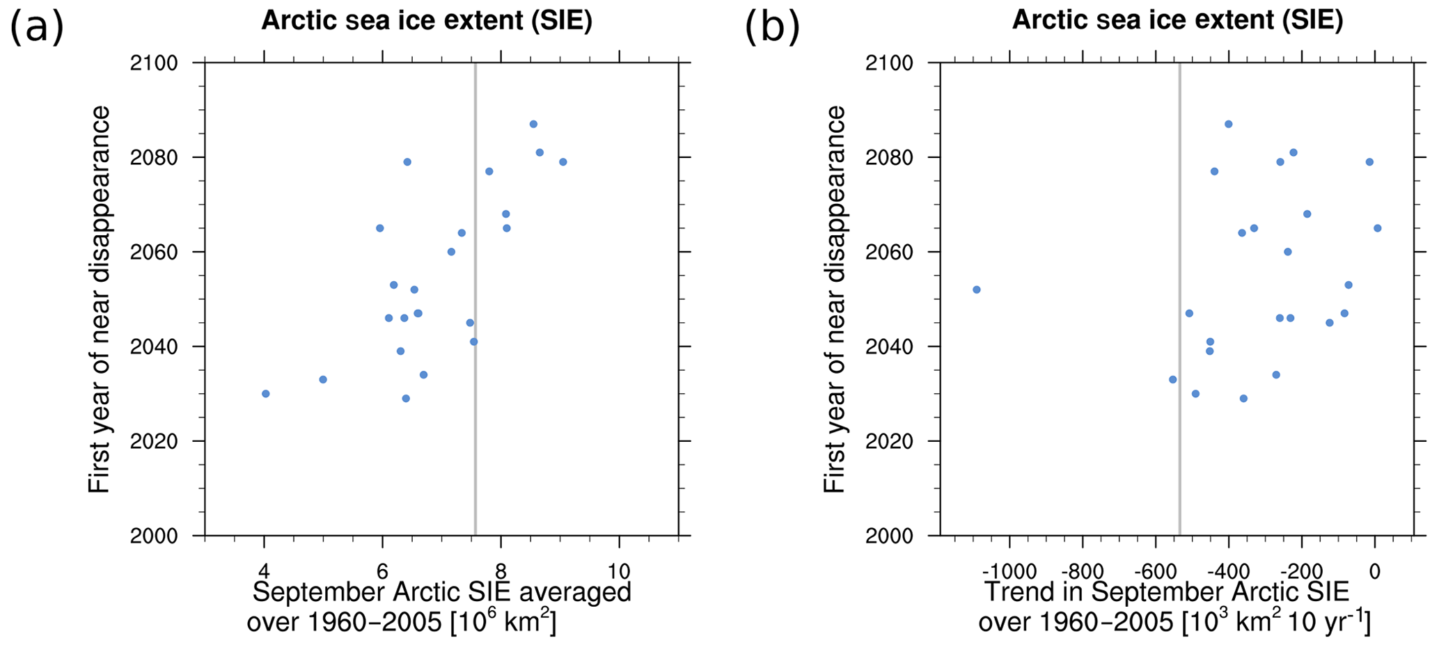
Figure 11Scatter plot of (a) mean historical (1960–2005) September Arctic sea ice extent (SSIE, million km2) and (b) trend in September Arctic sea ice extent (1960–2005) vs. first year of disappearance for scenario RCP8.5. The vertical gray lines are calculated from observations (HadISST, Rayner et al., 2003), similar to Fig. 12.31a/d of Collins et al. (2013). For details on recipe_seaice.yml, see Sect. 3.3.3.
3.3.4 Emergent constraints on the snow-albedo effect
The recipe recipe_snowalbedo.yml computes springtime snow-albedo feedback values in climate change vs. springtime values in the seasonal cycle in transient climate change experiments following Hall and Qu (2006). The strength of the snow-albedo effect is quantified by the variation in net incoming shortwave radiation (Q) with surface air temperature (Ts) due to changes in surface albedo αs:
Here, It is the constant incoming solar radiation at the top of the atmosphere, αp the planetary albedo. The diagnostic produces scatter plots of simulated springtime Δαs∕ΔTs values in climate change (ordinate) vs. simulated springtime Δαs∕ΔTs values in the seasonal cycle (abscissa). These values are calculated as follows:
-
(ordinate values) the change in April αs (future projection – historical) averaged over NH land masses poleward of 30∘ N is divided by the change in April Ts (future projection – historical) averaged over the same region. The change in αs (or Ts) is defined as the difference between 22nd century mean αs (Ts) and 20th-century-mean αs. Values of αs are weighted by April incoming insolation (It) prior to averaging.
-
The seasonal cycle Δαs∕ΔTs values (abscissa values), based on 20th century climatological means, are calculated by dividing the difference between April and May αs (averaged over NH continents poleward of 30∘ N) by the difference between April and May Ts averaged over the same area. Values of αs are weighted by April incoming insolation prior to averaging.
Figure 12 shows an example calculated from CMIP5 historical (1901–2000) and Representative Concentration Pathways 4.5 (RCP4.5, 2101–2200) experiments for 12 different models. The seasonal cycle values used as reference (vertical gray line) are calculated from the third generation of ISCCP radiative fluxes (ISCCP-FH; Young et al., 2018) and near-surface air temperature from ERA-Interim (Dee et al., 2011) for the years 1984–2000. While data from ISCCP-FH data suggest that CMIP5 models tend to underestimate springtime snow-albedo effect values in climate change, using the second generation of ISCCP radiative fluxes (ISCCP-FD, Zhang et al., 2004, not shown) as in Fig. 9.45a of Flato et al. (2013) suggests that the CMIP5 models under- and overestimate springtime snow-albedo effect almost equally.
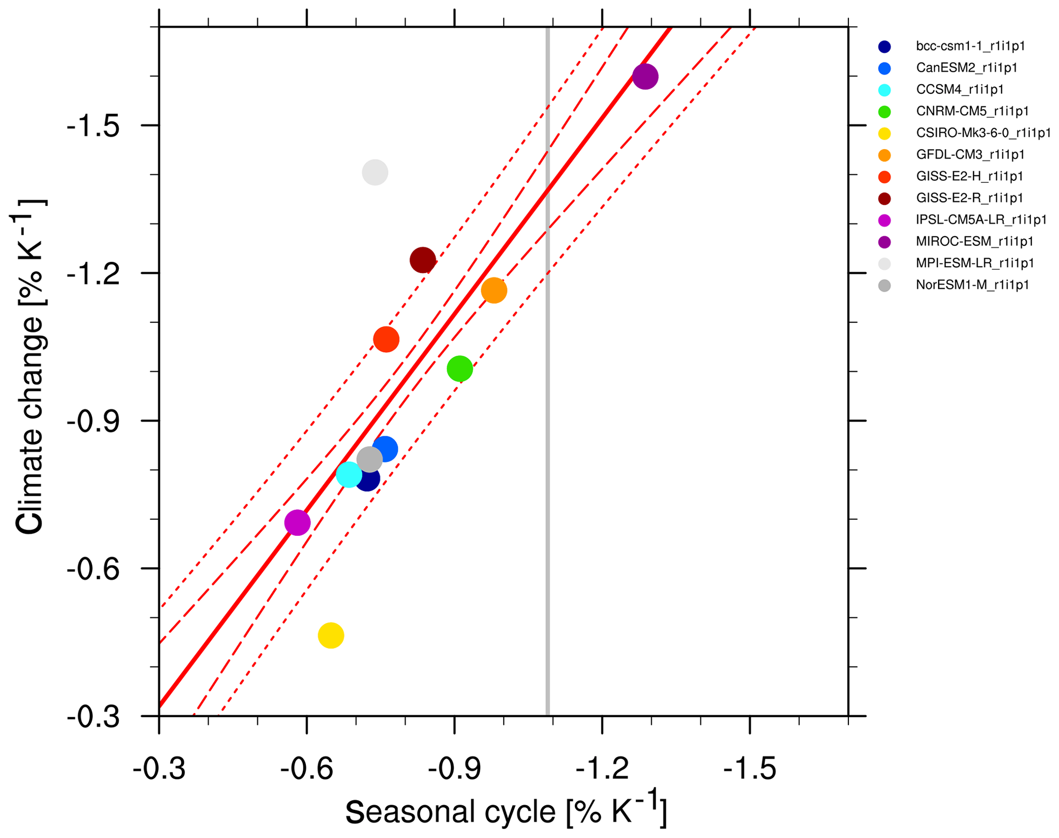
Figure 12Scatter plot of springtime snow-albedo effect values in climate change (ordinate) vs. springtime Δαs∕ΔTs values in the seasonal cycle (abscissa) in transient climate change experiments calculated from CMIP5 historical (1901–2000) and RCP4.5 (2101–2200) experiments. The vertical gray line shows the seasonal cycle values calculated from third generation of ISCCP radiative fluxes (ISCCP-FH, Young et al., 2018) and near-surface air temperature from ERA-Interim (Dee et al., 2011) for the years 1984–2000. Models with higher surface albedos over NH continents poleward of 30∘ N typically have a larger contrast between snow-covered and snow-free areas, and hence a stronger snow-albedo feedback. Similar to Fig. 9.45a of Flato et al. (2013); for details on recipe_snowalbedo.yml, see Sect. 3.3.4.

Figure 13The atmospheric energy budget (DeAngelis et al., 2015): (a) net atmospheric longwave cooling to the surface and outer space calculated as sum of upward longwave radiative flux at TOA and net downward longwave flux at the surface (rlnst), heating from shortwave absorption (rsnst), latent heat release from precipitation (lvp) and global average multi-model mean sensible heat flux (hfss). The panel shows three model experiments: the pre-industrial control simulation averaged over 150 years (blue), the RCP8.5 scenario averaged over 2091–2100 (orange) and the abrupt quadrupled CO2 scenario averaged over years 141–150 after CO2 quadrupling in all models except IPSL-CM5A-MR, for which the average is calculated over years 131–140 (gray). (b) The 95 % confidence interval for the slope of the regression of clear-sky rsnst normalized by the incoming shortwave flux at TOA with the water vapor path (prw) over the tropical ocean (30∘ S–30∘ N), regridded to a 2.5∘ latitude × 2 kg m−2 prw grid for different CMIP5 models (horizontal bars) and for data from CERES-EBAF (Kato et al., 2013; Loeb et al., 2009, rsnst) and RSS version-7 microwave radiometer data (Wentz et al., 2007, prw) together with ERA-Interim (Dee et al., 2011, prw) (dotted lines). The colors indicate different parameterization schemes for solar absorption by water vapor in a cloud-free atmosphere implemented in the models. Similar to Figs. 1b and 4 from DeAngelis et al. (2015) and produced with recipe_deangelis15nat.yml (see details in Sect. 3.3.5).
3.3.5 Emergent constraints on the hydrological cycle
The recipes recipe_deangelis2015nat.yml and recipe_li2017natcc.yml, newly developed for v2.0, reproduce the analysis from DeAngelis et al. (2015) and Li et al. (2017), respectively. DeAngelis et al. (2015) constrain the hydrologic cycle intensification with observed radiative fluxes and water vapor data. The recipe recipe_deangelis2015nat.yml reproduces their Figs. 1b (Fig. 13a) to 4 (Fig. 13b) as well as their extended data Figs. 1 and 2. Here, the analysis is shown for 17 CMIP5 models and includes monthly mean total precipitable water on a 1∘ × 1∘ grid from RSS (Remote Sensing System) version-7 microwave radiometer data (Wentz et al., 2007) and ERA-Interim reanalysis (Dee et al., 2011), as well as radiative fluxes from the Clouds and the Earth's Radiant Energy System Energy Balance and Filled (CERES-EBAF; Kato et al., 2013; Loeb et al., 2009) dataset. Figure 13a shows that energy sources and sinks readjust in reply to an increase in greenhouse gases, leading to a decrease in the sensible heat flux and an increase in the other fluxes; Fig. 13b shows that results from parameterization schemes using pseudo-k distributions with more than 20 exponential terms representing water vapor absorption and correlated-k distributions agree better with the observations than the other schemes.
Li et al. (2017) relate the future Indian summer monsoon projections to the present-day precipitation over the tropical western Pacific. With this relationship, they can correct the projected rainfall for models with too strong negative cloud–radiation feedback on sea surface temperature. The corrected values (see Fig. 14) do not show an increase in rainfall over the whole Indian summer monsoon (ISM) region under greenhouse warming and are expected to be more robust than the uncorrected projection (Li et al., 2017). The recipe_li2017natcc.yml reproduces their Figs. 1 and 2 for an ensemble of 22 CMIP5 models (Fig. 14) and their Fig. 1a for each of the individual models and the multi-model mean.
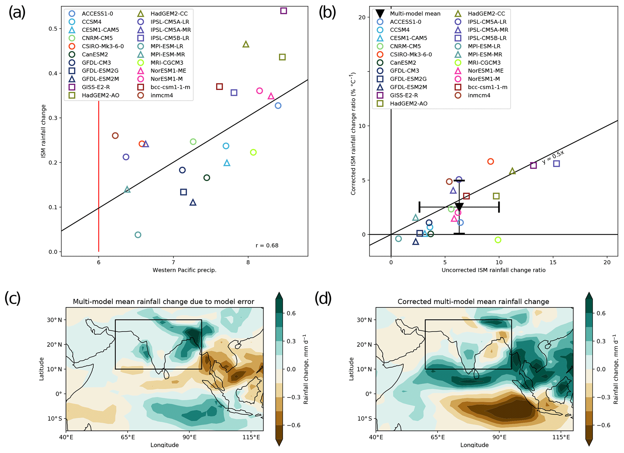
Figure 14Correction of the Indian summer monsoon (ISM; 10–30∘ N, 60–95∘ E) rainfall projected by models for the RCP8.5 scenario based on the bias in present-day precipitation over the tropical western Pacific (12∘ S–12∘ N, 140∘ E–170∘ W). (a) Scatter plot and the linear regression (black line, with the correlation coefficient r) of the western Pacific precipitation (mm d−1) from the CMIP5 historical simulations (1980–2005) and the ISM rainfall change between historical and RCP8.5 for the years 2070–2099 for different CMIP5 models. The red line indicates the present-day value for the western Pacific precipitation from observations as used in Li et al. (2017) estimated from the Global Precipitation Climatology Project (GPCP) dataset for 1980–1999 (Adler et al., 2003). (b) Uncorrected ISM rainfall change ratio (% per ∘C) vs. the corrected ratio from CMIP5 models and the multi-model mean with the standard deviations shown as error bars. The rain data are normalized by the global mean near-surface temperature change. (c) Projected multi-model mean rainfall change errors and (d) corrected multi-model mean rainfall change over the Indian Ocean. Similar to Fig. 2 of Li et al. (2017) and produced with recipe_li2017natcc.yml (see details in Sect. 3.3.5).
3.4 Climate model projections
In addition to the emergent constraints described in the previous section, ESMValTool v2.0 also includes new diagnostics specifically designed to analyze future climate projections from ESMs. This includes diagnostics using the multiple diagnostic ensemble regression used to constrain the future position of the austral jet, a “toy model” to allow for investigating the effect of observational uncertainty on model evaluation, diagnostics for reproducing selected figures from the climate projection chapter in IPCC AR5 (Collins et al., 2013) and for analyzing future sea ice quantities. All of these new diagnostics in ESMValTool v2.0 are briefly described in the following sections.
3.4.1 MDER to constrain future austral jet position
The position of the austral jet stream is poorly modeled by CMIP5 models with a latitude range of 10∘ within the ensemble and a mean bias towards the Equator. The recipe_wenzel16jclim.yml reproduces the study of Wenzel et al. (2016b) who used a process-oriented multiple diagnostic ensemble regression (MDER) to constrain the future jet position in the RCP4.5 scenario. MDER uses a stepwise regression scheme to identify the most relevant present-day diagnostics from a list of diagnostics provided as an input and links those to future projections via a multivariate linear regression scheme. With the diagnostics selected by MDER, the future quantity (in this case, the austral jet position) can be constrained with suitable observationally based data (here: ERA-Interim; Dee et al., 2011), following the same basic idea as emergent constraints (see also Sect. 3.3). Using this approach, the future jet position from CMIP5 models is bias corrected about 1.5∘ southwards compared to the unweighted multi-model mean (Fig. 15).
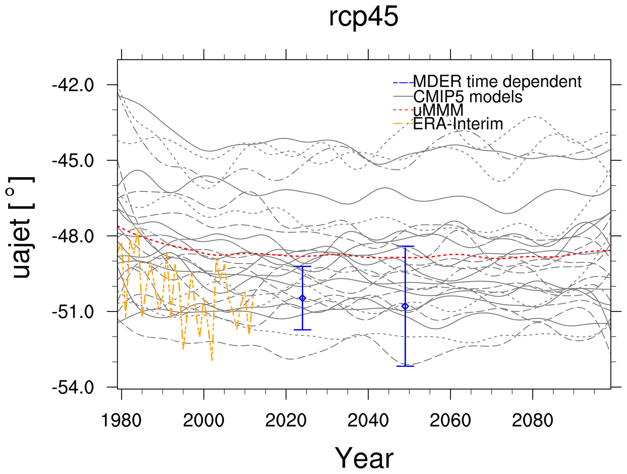
Figure 15Time series of the austral jet position for the RCP4.5 scenario between 1980 and 2100 based on Wenzel et al. (2016b). The gray lines show individual CMIP5 models and the dotted red line the unweighted CMIP5 multi-model mean (uMMM). Observationally based estimates of the jet position from ERA-Interim (Dee et al., 2011) are represented by the dashed yellow line. Blue error bars indicate the predicted jet position by the MDER analysis (multiple diagnostic ensemble regression) for the near-term future (2015–2034) and the midterm future (2040–2059). Similar to Fig. 5 of Wenzel et al. (2016b) and produced with recipe_wenzel16jclim.yml; see details in Sect. 3.4.1.
3.5 Toy model
Synthetic datasets generated from “toy models” have been used in the literature for assessing the effectiveness of multi-model combination strategies and for estimating the effect of observational uncertainties on the correlation between forecasts and observational datasets (Massonnet et al., 2016). The toy model recipe implemented into ESMValTool v2.0 is based on the approach presented in Weigel et al. (2008) for simulating single-model ensembles from a Gaussian distribution, where the number of members and the standard deviation of the error are defined by the user. Following Weigel et al. (2008), the recipe takes as input a set of observations, y1, y2, …, yN and for each observation yi, M synthetic members x are generated from
where , and ϵ1, …, with the notation N(μ,σ) referring to a random number drawn from a normal distribution with mean μ and standard deviation σ. The simulated value xm is obtained by multiplying y by α, the predictability of the observation, which is set to 1 in this instance, and by adding a vector of perturbations ϵm and the scalar perturbation ϵβ. The simulated values have the following properties:
-
The simulated values xi,1 have the same climatology as the observations.
-
The mean correlation between the simulations xi,1, …, xi,M and observation yi is determined by α (see toy model properties described in Weigel et al., 2008).
-
The parameter β describes the model underdispersion, where β=0 corresponds to the case where the synthetic ensemble is well dispersed and covers the full range of uncertainties for a given correlation α. The underdispersion increases with β being limited to the range .
Parameter β is introduced to control the dispersion. For well-dispersed ensembles, skill is independent of the number of simulations involved, while for overconfident model ensembles, skill grows with the ensemble size. Given that β accounts for the dispersion, this approach leads α to represent a measure of predictability (Weigel et al., 2008).
This toy model is based on very simplifying assumptions: (1) normality and stationarity: the climatology and the ensemble distributions are assumed to be stationary and normally distributed; (2) well-calibrated model climatology: each ensemble member has the same climatology as the observations; (3) stationary skill: spread and correlation do not vary from sample to sample; (4) predictable signal and observational errors: requires the signal to be given by αx, and therefore it is determined by the verifying observation (Weigel et al., 2008).
The predictability α is 1 since we are only interested in generating synthetic observations. Thus, the user only needs to define the standard deviation of the error. This term can be based on the observational uncertainty when available (e.g., as provided with the European Space Agency's Climate Change Initiative (ESA CCI) SST dataset; Merchant et al., 2014a, b) or estimated by the user, e.g., by calculating the standard deviation between different observational reference datasets (Bellprat et al., 2017).
We would like to note that in addition to the observational uncertainty itself, also spatiotemporal representativeness of observations plays an important role when evaluating models. Schutgens et al. (2017) showed that such representation errors remain even after spatial and temporal averaging and may be larger than typical measurement errors. In addition, also the calculation method of a quantity to be compared with observations can play an important role. This is, for example, the case when comparing satellite retrievals with model quantities that are not derived the same way. Application of satellite simulators such as the Cloud Feedback Model Intercomparison Project (CFMIP) Observation Simulator Package (COSP; Bodas-Salcedo et al., 2011) can help to reduce such uncertainties in model evaluation. Both of these aspects are not covered by the toy model, which only provides an estimate for the observational uncertainty itself.
For further discussion of this synthetic value generator, its general application to forecasts and its limitations, see Weigel et al. (2008). The recipe recipe_toymodel.yml writes a NetCDF file containing the synthetic observations. Due to the sampling of the perturbations from a Gaussian distribution, running the recipe multiple times, with the same observation dataset and input parameters, will result in different outputs (Fig. 16).
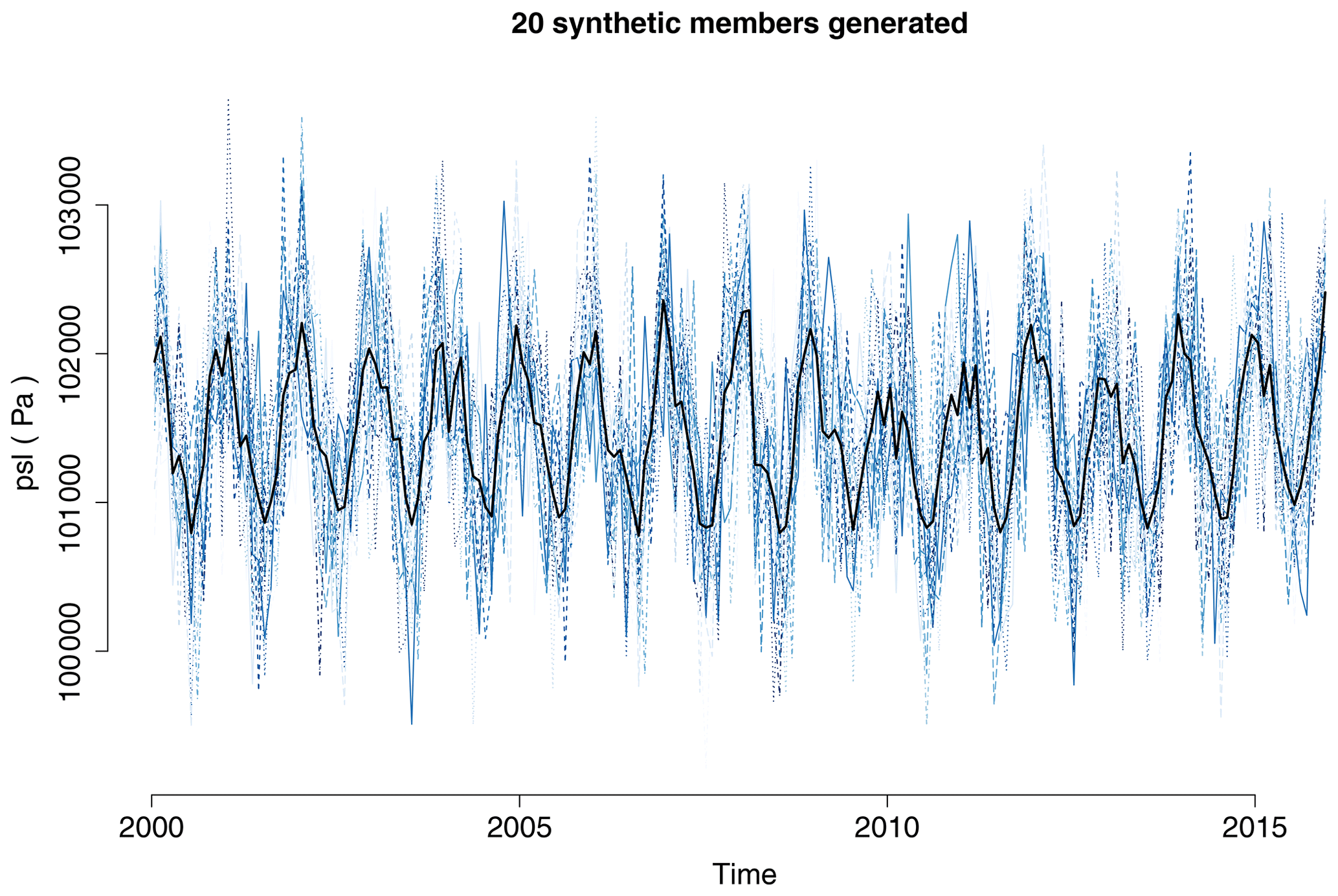
Figure 16Example of 20 synthetic members of a single dataset ensemble generated by recipe_toymodel.yml. Shown are time series of surface-level pressure (psl) averaged over the region 30–50∘ N, 40∘ E–40∘ W, from 2000 to 2015, created from monthly mean data from ERA-Interim (Dee et al., 2011). With the user providing an estimate for the standard error, e.g., from differences between different observational datasets, this diagnostic can be used to investigate the effect of observational uncertainty. For details, see Sect. 3.4.2.
3.5.1 Climate projection chapter of IPCC WGI AR5
The recipe_collins13ipcc.yml reproduces a subset of the figures from the long-term climate change projections chapter of the IPCC AR5 (chapter 12, Collins et al., 2013). This new recipe in version 2.0 allows for reproduction of selected figures from AR5 to show changes between historical and future projections over the available CMIP models. It will also allow a faster analysis of the CMIP6 climate projections that are part of the Scenario Model Intercomparison Project (ScenarioMIP; O'Neill et al., 2016). The recipe includes figures such as time series from historical periods to projections (including spread among models; see Fig. 17), horizontal maps for individual models as well as multi-model means (including stippling to indicate large changes with high model agreement and hatching to indicate areas with a small signal or low agreement of models; see Fig. 18) and vertical zonal mean plots (also including stippling and hatching to indicate significant changes). The example shown in Fig. 18 shows where the CMIP5 models project an increase in precipitation and where they project a decrease. This example also shows quite large regions where the projections are still uncertain; i.e., the multi-model mean signal is smaller than 1 standard deviation of the natural variability estimated from pre-industrial control simulations (hatching).
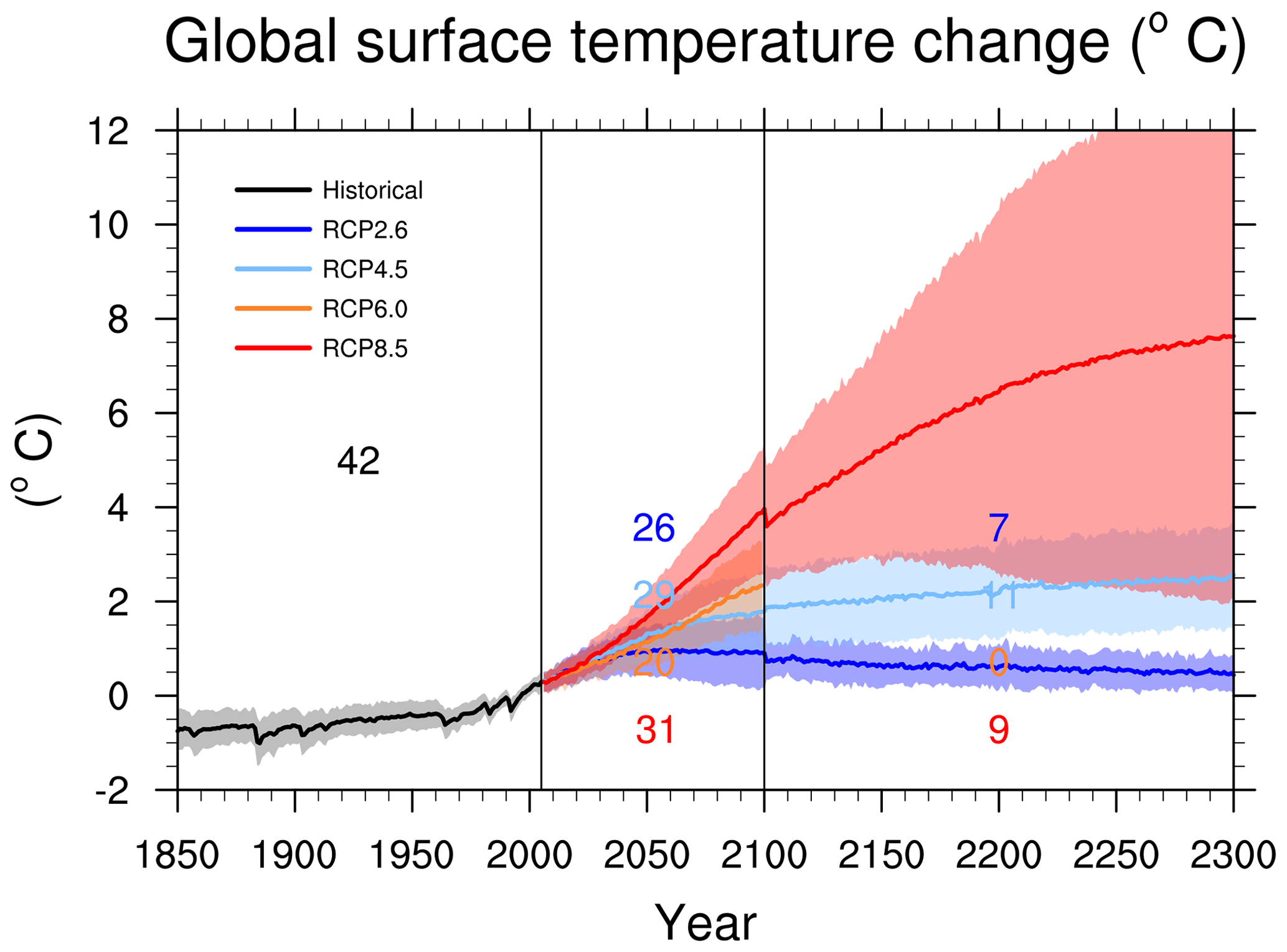
Figure 17Time series of global annual mean surface air temperature anomalies (relative to 1986–2005) from CMIP5 models and RCP2.6, 4.5, 6.0 and 8.5 scenarios. The solid lines show the multi-model mean; the shading shows the 5 % to 95 % range (±1.64 standard deviations). The numbers indicate the number of models these estimates are based on. Similar to Collins et al. (2013) Fig. 12.5 and produced with recipe_collins13ipcc.yml (see Sect. 3.4.3 for details).
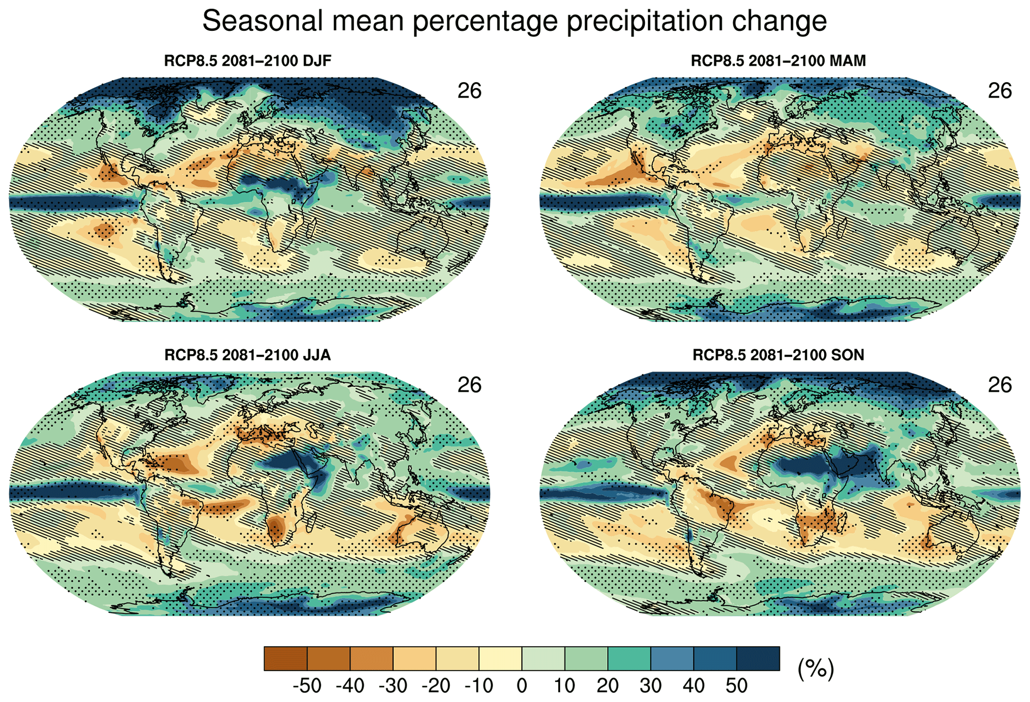
Figure 18Global maps of seasonal mean change in precipitation from 1986–2005 (reference period) to 2081–2100 for the RCP8.5 scenario. Hatching indicates regions where the multi-model mean change is less than 1 standard deviation of the internal variability estimated from piControl simulations. Stippling indicates regions where the multi-model mean change is greater than 2 standard deviations of the internal variability and where at least 90 % of models agree on the sign of the change. The numbers in the upper right of each panel indicate the number of models used. Similar to Fig. 12.22 of Collins et al. (2013) but only for one future time period. Produced with recipe_collins13ipcc.yml (see Sect. 3.4.3 for details).
Most diagnostics scripts are set up in a generic way, so that in principle they can be used for any variable from the CMIP archive. The scripts have been tested for the variables indicated in Table 1. To be able to determine if a change signal is larger than natural variability the natural variability is calculated from the piControl runs, other than that the recipe uses historical and RCP runs. All diagnostics in this recipe with the exception of the emergent constraints on the year of disappearance of September Arctic sea ice (Sect. 3.3.3) do not use observations.
3.5.2 Sea ice
The sea ice diagnostics included in the ESMValTool (recipe_seaice.yml) have been extended with three new diagnostics. The first new diagnostic (seaice_trends.ncl) calculates the trend in sea ice extent or sea ice area from each model and reference observation(s) or reanalysis data that are given in the recipe. The diagnostic produces histogram plots of the trend distributions from all models and adds the reference datasets (here: HadISST; Rayner et al., 2003) as colored vertical lines. The user can specify the region (Arctic or Antarctic) and the month of the year for which sea ice area/extent is calculated. The trends are calculated over the full period specified in the recipe and the resulting plots are similar to those of Fig. 9.24c/d in Flato et al. (2013) . The example plot (Fig. 19) shows that the majority of CMIP5 models slightly underestimate the observed trend in summer sea ice extent over the time period of 1960–2005.
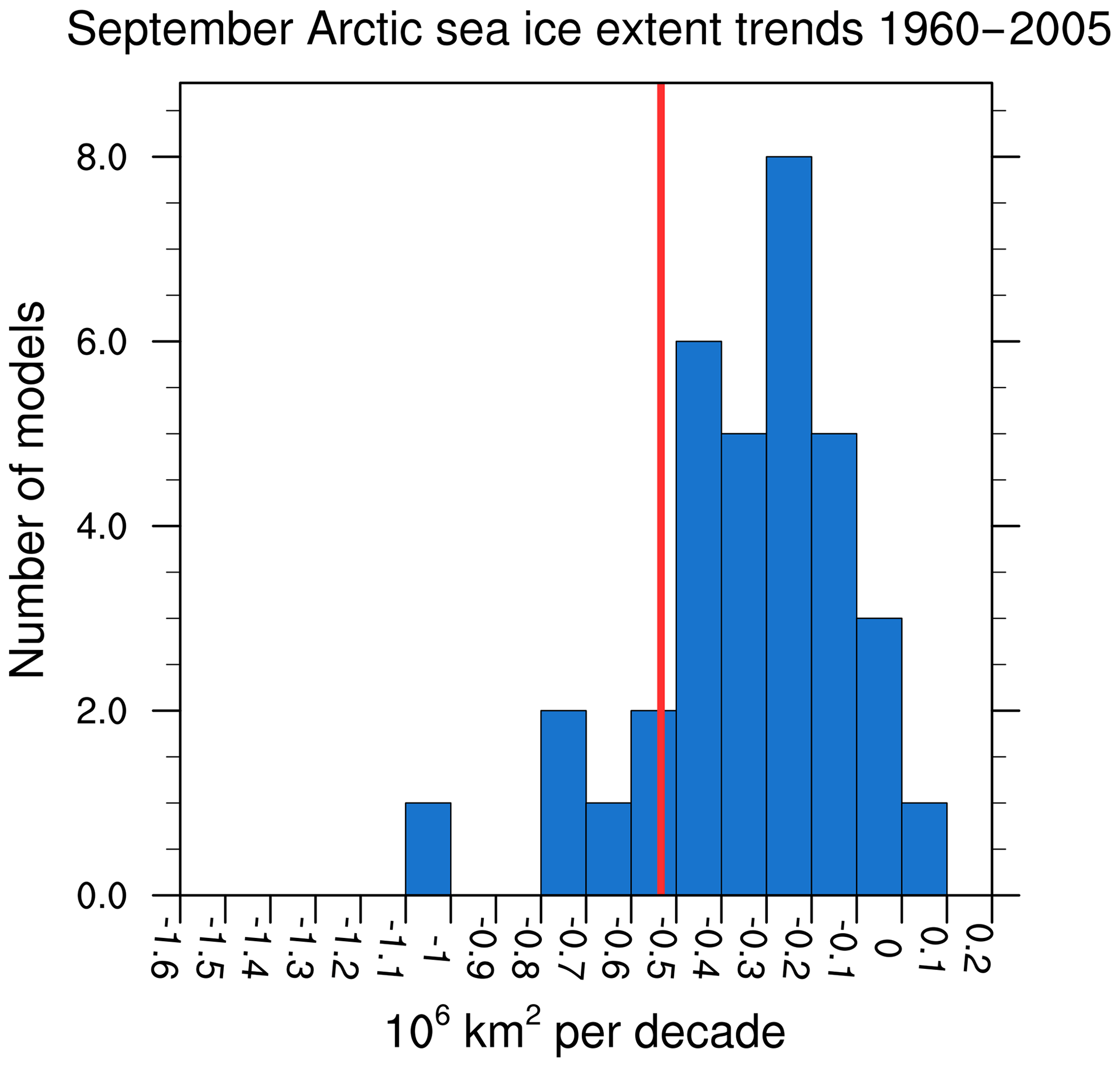
Figure 19Distribution of trends in September Arctic sea ice extent calculated from the historical simulations (1960–2005) of 26 CMIP5 models (similar to Flato et al., 2013, Fig. 9.24c). An observational estimate of the trend in summer sea ice extent from HadISST (Rayner et al., 2003) over the same time period is shown by the vertical red line. Produced with recipe_seaice.yml; for details, see Sect. 3.4.4.
The second new diagnostic (seaice_yod.ncl) calculates the year of near disappearance of Arctic sea ice. The diagnostic creates a time series plot of September Arctic sea ice extent for each model given in the recipe and adds three multi-model statistics: mean, standard deviation and YOD. It optionally reads a list of pre-calculated model weights and adds the weighted multi-model mean time series including weighted multi-model standard deviation to the plot (see, for example, Fig. 7 of Senftleben et al., 2020). The example in Fig. 20 shows that there is a large spread in simulated sea ice extent among the CMIP5 models with individual models simulating a summer sea ice extent below 1 million km2 already around the year 2025, while other models are still well above this threshold in 2100.
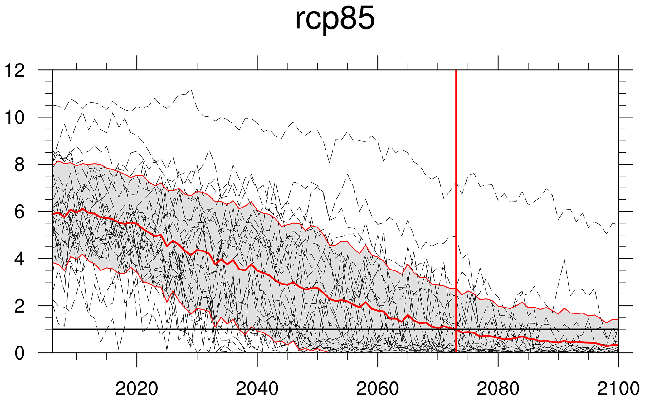
Figure 20Time series of September Arctic sea ice extent for individual CMIP5 models (dashed gray lines), multi-model mean (thick red line) and multi-model standard deviation (area shaded between thin red lines) for scenario RCP8.5. The year of disappearance (sea ice extent below 1 million km2) obtained from the CMIP5 multi-model mean is indicated by the vertical red line (similar to Collins et al., 2013, Fig. 12.31e). Produced with recipe_seaice.yml; for details, see Sect. 3.4.4.
The third new diagnostic (seaice_ecs.ncl) calculates emergent constraints for YOD using mean or trend in sea ice extent. The diagnostic produces scatter plots of different historical and future sea ice metrics, similar to those in Fig. 2 of Massonnet et al. (2012) and Fig. 12.31a/c of Collins et al. (2013) (see Sect. 3.3.3 for details).
In this article, diagnostics and metrics, newly implemented into the Earth System Model Evaluation Tool v2.0 to analyze projections from ESMs and emergent constraints for climate-relevant parameters including effective climate sensitivity, snow-albedo effect, climate–carbon cycle feedback, hydrologic cycle intensification, future Indian summer monsoon precipitation, land photosynthesis and year of disappearance of summer Arctic sea ice, are described and illustrated with examples using CMIP5 data.
The implemented multi-model products allow for an easy and quick overview of the multi-model ensemble mean and the inter-model agreement in the sign of the multi-model mean anomaly for a given variable, geographical region, season and time period. In addition to maps showing the anomalies and their inter-model agreement, the results are also given as anomaly time series showing each individual model and the multi-model ensemble mean, which can be used to estimate the inter-model spread.
ECS and TCR are climate metrics that can be used to estimate and compare the sensitivity of simulated near-surface temperature from individual models to increased atmospheric CO2 concentrations. With these metrics included in the ESMValTool, it is easily possible to group the models in high- and low-sensitivity models for further analysis.
Emergent constraints offer the possibility to use an ensemble of ESMs together with observations in order to constrain non-observable parameters such as simulated future Earth system feedbacks. Overall, seven emergent constraints are available in ESMValTool v2.0 for ECS: (1) covariance of shortwave cloud reflection using the models' correlation of the covariance of tropical low-level cloud reflection with the underlying SST (Brient and Schneider, 2016); (2) latitude of the climatological mean Hadley cell edge (Lipat et al., 2017); (3) atmospheric convective mixing calculated as sum of small- and large-scale component, the lower tropospheric mixing index (Sherwood et al., 2014); (4) bias in climatological annual mean precipitation over the southeastern Pacific, the southern ITCZ index (Tian, 2015); (5) mid-tropospheric humidity over the tropical Pacific, the tropical mid-tropospheric humidity asymmetry index (Tian, 2015); (6) global temperature variability (Cox et al., 2018); and (7) difference between tropical and midlatitude cloud fraction (Volodin, 2008). Two emergent constraints on the hydrological cycle are implemented: (1) a constraint on the hydrological cycle intensification that uses observations of radiative fluxes and water vapor (DeAngelis et al., 2015); and (2) a constraint on the future Indian summer monsoon using present-day precipitation data over the tropical western Pacific (Li et al., 2017). Additionally, emergent constraints are available for the carbon cycle: (1) future tropical land carbon storage (Wenzel et al., 2014); (2) projected land photosynthesis (Wenzel et al., 2016a). Also implemented are emergent constraints for the year of disappearance of September Arctic sea ice (Massonnet et al., 2012) and for the snow-albedo effect (Hall and Qu, 2006).
Various new diagnostics are available specifically for analysis of climate model projections. The MDER method has been implemented to constrain the projected position of the austral jet following Wenzel et al. (2016b). The method uses a stepwise regression to identify the most relevant diagnostics (calculated with present-day data) that are linked to projections of a quantity via a multivariate linear regression scheme. Observational data can then be used to constrain the projected quantity such as the future austral jet position.
A number of newly implemented diagnostics resembling selected figures from IPCC AR5 chapter 12 (Collins et al., 2013) for analysis of climate model projections are grouped in one recipe. The diagnostics include time series and horizontal maps and vertical zonal maps including stippling and hatching to show significant changes between a climate projection scenario and a historical simulation. For the stippling and hatching, results from pre-industrial control runs are used to estimate internal variability of a variable, which is then used to assess whether simulated changes are significant or not. Diagnostics to analyze sea ice in climate model simulations are also grouped in one recipe. The new diagnostics include calculation of trends in sea ice area and extent, multi-model estimates for the year of disappearance of sea ice in climate projections and scatter plots of different historical and future sea ice metrics such as historical trend in sea ice extent vs. YOD. In addition, a “toy model” has been implemented into ESMValTool v2.0 that allows generating synthetic ensemble members from a single dataset (Weigel et al., 2008). When applied to observational data, this can be used to take into account observational uncertainty when comparing the observations with model results. For this, the user needs to specify the standard error of the observations that is provided with some observational datasets or estimated from differences between different observational datasets for the same quantity.
ESMValTool v2.0 is an open-source software tool that has been specifically developed to facilitate evaluation and analysis of Earth system models participating in CMIP. As such, it can process and analyze CMOR compliant model output and observational datasets with the particular aim to provide traceable and reproducible results, well-documented diagnostics and metrics and an efficient workflow allowing to evaluate models in more depth and more rapidly than it was typically possible in previous CMIP phases. The CMOR standard is, however, quite detailed and implemented in a relatively strict way in the ESMValTool in order to ensure data consistency and to minimize the probability of errors in the data processing. Increasing the flexibility of the CMOR check and automatic fixes of small inconsistencies is a currently ongoing activity and should make the data processing smoother, especially for datasets which are not part of CMIP or any CMIP-endorsed model intercomparison project (MIP). This means that a certain familiarity with these data standards is required in order to use the ESMValTool. Another limitation is that for license issues, observations cannot be distributed together with the software package. New users are required to download and process observational datasets before being able to use the tool or to have access to a computing center where observational data for the ESMValTool (i.e., CMORized) are already available. We are currently working on automating this process to facilitate the data retrieval and CMORization process.
The new ESMValTool is now available to the community for evaluation and scientific analyses of CMIP6 data. Thanks to a strong community involvement, the ESMValTool is constantly extended and improved in an effort to make the tool more user friendly, more efficient and a better tool for climate analyses. The ongoing ESMValTool development and discussions regarding new features can be followed on GitHub at https://github.com/ESMValGroup (last access: 1 September 2020). Feedback, bug reports and contributions by the scientific community are very welcome at any time.
ESMValTool v2.0 is released under the Apache License, VERSION 2.0. The latest release of ESMValTool v2.0 is publicly available on Zenodo at https://doi.org/10.5281/zenodo.3970975 (Andela et al., 2020a). The source code of the ESMValCore package, which is installed as a dependency of ESMValTool v2.0, is also publicly available on Zenodo at https://doi.org/10.5281/zenodo.3952695 (Andela et al., 2020b). ESMValTool and ESMValCore are developed on the GitHub repositories available at https://github.com/ESMValGroup (last access: 1 September 2020).
CMIP5 data are available freely and publicly from the Earth System Grid Federation (ESGF). Observations used in the evaluation are detailed in the various sections of the paper. The observational datasets are not distributed with the ESMValTool that is restricted to the code as open-source software. Observational datasets that are available through the Observations for Model Intercomparisons Project (obs4MIPs, https://esgf-node.llnl.gov/projects/obs4mips/, last access: 26 February 2020) can be downloaded freely from the ESGF and directly used in the ESMValTool. For all other observational datasets, the ESMValTool provides a collection of scripts (NCL and Python) with exact downloading and processing instructions to recreate the datasets used in this publication.
AL and VE coordinated the ESMValTool v2.0 diagnostic effort and led the writing of the paper. MR helped coordinate the diagnostic implementation and testing in ESMValTool v2.0. All other authors contributed individual diagnostics to this release. All authors contributed to the text.
The authors declare that they have no conflict of interest.
The development of ESMValTool (v2.0) is supported by several projects. The diagnostic development of ESMValTool v2.0 for this paper was supported by different projects with different scientific focus, in particular by (1) the European Union's Horizon 2020 Framework Programme for Research and Innovation “Coordinated Research in Earth Systems and Climate: Experiments, kNowledge, Dissemination and Outreach (CRESCENDO)” project under grant agreement no. 641816, (2) the European Union's Horizon 2020 project “Climate-Carbon Interactions in the Coming Century” (4C) under grant agreement no. 821003, (3) Copernicus Climate Change Service (C3S) “Metrics and Access to Global Indices for Climate Projections (C3S-MAGIC)” project, (4) Federal Ministry of Education and Research (BMBF) CMIP6-DICAD project, (5) ESA Climate Change Initiative Climate Model User Group (ESA CCI CMUG) and (6) Helmholtz Society project “Advanced Earth System Model Evaluation for CMIP (EVal4CMIP)”. In addition, we received technical support on the ESMValTool v2.0 development from the European Union's Horizon 2020 Framework Programme for Research and Innovation “Infrastructure for the European Network for Earth System Modelling (IS-ENES3)” project under grant agreement no. 824084.
We acknowledge the World Climate Research Program's (WCRP's) Working Group on Coupled Modelling (WGCM), which is responsible for CMIP, and we thank the climate modeling groups for producing and making available their model output. We thank Franziska Winterstein (DLR) for her helpful comments on the manuscript. The computational resources of the Deutsches Klimarechenzentrum (DKRZ, Germany) were essential for developing and testing this new version and are kindly acknowledged.
This research has been supported by the Horizon 2020 Framework Programme
(CRESCENDO (grant no. 641816), 4C (grant no. 821003), and IS-ENES3 (grant no. 824084)), the Copernicus Climate Change
Service (C3S) (Metrics and Access to Global Indices for Climate Change Projections (MAGIC)),
the Federal Ministry of Education and Research (BMBF) (CMIP6-DICAD), the European
Space Agency (ESA Climate Change Initiative Climate Model User Group (ESA CCI CMUG)) and the
Helmholtz Association (Advanced Earth System Model Evaluation for CMIP (EVal4CMIP)).
The article processing charges for this open-access
publication were covered by a Research
Centre of the Helmholtz Association.
This paper was edited by Fiona O'Connor and reviewed by two anonymous referees.
Adler, R. F., Huffman, G. J., Chang, A., Ferraro, R., Xie, P. P., Janowiak, J., Rudolf, B., Schneider, U., Curtis, S., Bolvin, D., Gruber, A., Susskind, J., Arkin, P., and Nelkin, E.: The version-2 global precipitation climatology project (GPCP) monthly precipitation analysis (1979–present), J. Hydrometeorol., 4, 1147–1167, 2003.
Andela, B., Broetz, B., de Mora, L., Drost, N., Eyring, V., Koldunov, N., Lauer, A., Mueller, B., Predoi, V., Righi, M., Schlund, M., Vegas-Regidor, J., Zimmermann, K., Adeniyi, K., Arnone, E., Bellprat, O., Berg, P., Bock, L., Caron, L.-P., Carvalhais, N., Cionni, I., Cortesi, N., Corti, S., Crezee, B., Davin, E. L., Davini, P., Deser, C., Diblen, F., Docquier, D., Dreyer, L., Ehbrecht, C., Earnshaw, P., Gier, B., Gonzalez-Reviriego, N., Goodman, P., Hagemann, S., von Hardenberg, J., Hassler, B., Hunter, A., Kadow, C., Kindermann, S., Koirala, S., Lledó, L., Lejeune, Q., Lembo, V., Little, B., Loosveldt-Tomas, S., Lorenz, R., Lovato, T., Lucarini, V., Massonnet, F., Mohr, C. W., Amarjiit, P., Pérez-Zanón, N., Phillips, A., Russell, J., Sandstad, M., Sellar, A., Senftleben, D., Serva, F., Sillmann, J., Stacke, T., Swaminathan, R., Torralba, V., and Weigel, K.: ESMValTool (Version v2.0.0), Zenodo, https://doi.org/10.5281/zenodo.3970975, 2020a.
Andela, B., Broetz, B., de Mora, L., Drost, N., Eyring, V., Koldunov, N., Lauer, A., Predoi, V., Righi, M., Schlund, M., Vegas-Regidor, J., Zimmermann, K., Bock, L., Diblen, F., Dreyer, L., Earnshaw, P., Hassler, B., Little, B., and Loosveldt-Tomas, S.: ESMValCore (Version v2.0.0), Zenodo, https://doi.org/10.5281/zenodo.3952695, 2020b.
Bellprat, O., Massonnet, F., Siegert, S., Prodhomme, C., Macias-Gómez, D., Guemas, V., and Doblas-Reyes, F. J. R. S. O. E.: Uncertainty propagation in observational references to climate model scales, Remote Sens. Environ., 203, 101–108, 2017.
Bellucci, A., Gualdi, S., and Navarra, A. J. J. O. C.: The double-ITCZ syndrome in coupled general circulation models: the role of large-scale vertical circulation regimes, J. Climate, 23, 1127–1145, 2010.
Bodas-Salcedo, A., Webb, M. J., Bony, S., Chepfer, H., Dufresne, J. L., Klein, S. A., Zhang, Y., Marchand, R., Haynes, J. M., Pincus, R., and John, V. O.: COSP Satellite simulation software for model assessment, B. Am. Meteorol. Soc., 92, 1023–1043, 2011.
Brient, F. and Schneider, T.: Constraints on Climate Sensitivity from Space-Based Measurements of Low-Cloud Reflection, J. Climate, 29, 5821–5835, 2016.
Collins, M., Knutti, R., Arblaster, J., Dufresne, J.-L., Fichefet, T., Friedlingstein, P., Gao, X., Gutowski, W. J., Johns, T., Krinner, G., Shongwe, M., Tebaldi, C., Weaver, A. J., and Wehner, M.: Long-term Climate Change: Projections, Commitments and Irreversibility, in: Climate Change 2013: The Physical Science Basis. Contribution of Working Group I to the Fifth Assessment Report of the Intergovernmental Panel on Climate Change, edited by: Stocker, T. F., Qin, D., Plattner, G.-K., Tignor, M., Allen, S. K., Boschung, J., Nauels, A., Xia, Y., Bex, V., and Midgley, P. M., Cambridge University Press, Cambridge, United Kingdom and New York, NY, USA, 2013.
Cox, P. M., Pearson, D., Booth, B. B., Friedlingstein, P., Huntingford, C., Jones, C. D., and Luke, C. M.: Sensitivity of tropical carbon to climate change constrained by carbon dioxide variability, Nature, 494, 341–344, 2013.
Cox, P. M., Huntingford, C., and Williamson, M. S. J. N.: Emergent constraint on equilibrium climate sensitivity from global temperature variability, Nature, 553, 319–322, 2018.
DeAngelis, A. M., Qu, X., Zelinka, M. D., and Hall, A.: An observational radiative constraint on hydrologic cycle intensification, Nature, 528, 249–253, 2015.
Dee, D. P., Uppala, S. M., Simmons, A. J., Berrisford, P., Poli, P., Kobayashi, S., Andrae, U., Balmaseda, M. A., Balsamo, G., Bauer, P., Bechtold, P., Beljaars, A. C. M., van de Berg, L., Bidlot, J., Bormann, N., Delsol, C., Dragani, R., Fuentes, M., Geer, A. J., Haimberger, L., Healy, S. B., Hersbach, H., Holm, E. V., Isaksen, L., Kallberg, P., Kohler, M., Matricardi, M., McNally, A. P., Monge-Sanz, B. M., Morcrette, J. J., Park, B. K., Peubey, C., de Rosnay, P., Tavolato, C., Thepaut, J. N., and Vitart, F.: The ERA-Interim reanalysis: configuration and performance of the data assimilation system, Q. J. Roy. Meteor. Soc., 137, 553–597, 2011.
Eyring, V., Bony, S., Meehl, G. A., Senior, C. A., Stevens, B., Stouffer, R. J., and Taylor, K. E.: Overview of the Coupled Model Intercomparison Project Phase 6 (CMIP6) experimental design and organization, Geosci. Model Dev., 9, 1937–1958, https://doi.org/10.5194/gmd-9-1937-2016, 2016a.
Eyring, V., Righi, M., Lauer, A., Evaldsson, M., Wenzel, S., Jones, C., Anav, A., Andrews, O., Cionni, I., Davin, E. L., Deser, C., Ehbrecht, C., Friedlingstein, P., Gleckler, P., Gottschaldt, K.-D., Hagemann, S., Juckes, M., Kindermann, S., Krasting, J., Kunert, D., Levine, R., Loew, A., Mäkelä, J., Martin, G., Mason, E., Phillips, A. S., Read, S., Rio, C., Roehrig, R., Senftleben, D., Sterl, A., van Ulft, L. H., Walton, J., Wang, S., and Williams, K. D.: ESMValTool (v1.0) – a community diagnostic and performance metrics tool for routine evaluation of Earth system models in CMIP, Geosci. Model Dev., 9, 1747–1802, https://doi.org/10.5194/gmd-9-1747-2016, 2016b.
Eyring, V., Cox, P. M., Flato, G. M., Gleckler, P. J., Abramowitz, G., Caldwell, P., Collins, W. D., Gier, B. K., Hall, A. D., and Hoffman, F. M. J. N. C. C.: Taking climate model evaluation to the next level, Nat. Clim. Change, 9, 102–110, 2019.
Eyring, V., Bock, L., Lauer, A., Righi, M., Schlund, M., Andela, B., Arnone, E., Bellprat, O., Brötz, B., Caron, L.-P., Carvalhais, N., Cionni, I., Cortesi, N., Crezee, B., Davin, E. L., Davini, P., Debeire, K., de Mora, L., Deser, C., Docquier, D., Earnshaw, P., Ehbrecht, C., Gier, B. K., Gonzalez-Reviriego, N., Goodman, P., Hagemann, S., Hardiman, S., Hassler, B., Hunter, A., Kadow, C., Kindermann, S., Koirala, S., Koldunov, N., Lejeune, Q., Lembo, V., Lovato, T., Lucarini, V., Massonnet, F., Müller, B., Pandde, A., Pérez-Zanón, N., Phillips, A., Predoi, V., Russell, J., Sellar, A., Serva, F., Stacke, T., Swaminathan, R., Torralba, V., Vegas-Regidor, J., von Hardenberg, J., Weigel, K., and Zimmermann, K.: Earth System Model Evaluation Tool (ESMValTool) v2.0 – an extended set of large-scale diagnostics for quasi-operational and comprehensive evaluation of Earth system models in CMIP, Geosci. Model Dev., 13, 3383–3438, https://doi.org/10.5194/gmd-13-3383-2020, 2020.
Flato, G., Marotzke, J., Abiodun, B., Braconnot, P., Chou, S. C., Collins, W., Cox, P., Driouech, F., Emori, S., Eyring, V., Forest, C., Gleckler, P., Guilyardi, E., Jakob, C., Kattsov, V., Reason, C., and Rummukainen, M.: Evaluation of Climate Models, in: Climate Change 2013: The Physical Science Basis. Contribution of Working Group I to the Fifth Assessment Report of the Intergovernmental Panel on Climate Change, edited by: Stocker, T. F., Qin, D., Plattner, G.-K., Tignor, M., Allen, S. K., Boschung, J., Nauels, A., Xia, Y., Bex, V., and Midgley, P. M., Cambridge University Press, Cambridge, United Kingdom and New York, NY, USA, 2013.
Friedlingstein, P., Cox, P., Betts, R., Bopp, L., Von Bloh, W., Brovkin, V., Cadule, P., Doney, S., Eby, M., Fung, I., Bala, G., John, J., Jones, C., Joos, F., Kato, T., Kawamiya, M., Knorr, W., Lindsay, K., Matthews, H. D., Raddatz, T., Rayner, P., Reick, C., Roeckner, E., Schnitzler, K. G., Schnur, R., Strassmann, K., Weaver, A. J., Yoshikawa, C., and Zeng, N.: Climate-carbon cycle feedback analysis: Results from the (CMIP)-M-4 model intercomparison, J. Climate, 19, 3337–3353, 2006.
Gregory, J. M. and Forster, P. M.: Transient climate response estimated from radiative forcing and observed temperature change, J. Geophys. Res.-Atmos., 113, D23105, https://doi.org/10.1029/2008JD010405, 2008.
Gregory, J. M., Ingram, W., Palmer, M., Jones, G., Stott, P., Thorpe, R., Lowe, J., Johns, T., and Williams, K. J. G. R. L.: A new method for diagnosing radiative forcing and climate sensitivity, Geophys. Res. Lett., 31, L03205, https://doi.org/10.1029/2003GL018747, 2004.
Hall, A. and Qu, X.: Using the current seasonal cycle to constrain snow albedo feedback in future climate change, Geophys. Res. Lett., 33, L03502, https://doi.org/10.1029/2005GL025127, 2006.
Hasselmann, K.: Stochastic climate models Part I. Theory, Tellus, 28, 473–485, 1976.
Hirota, N., Takayabu, Y. N., Watanabe, M., and Kimoto, M. J. J. O. C.: Precipitation reproducibility over tropical oceans and its relationship to the double ITCZ problem in CMIP3 and MIROC5 climate models, J. Climate, 24, 4859–4873, 2011.
Huffman, G. J., Bolvin, D. T., Nelkin, E. J., Wolff, D. B., Adler, R. F., Gu, G., Hong, Y., Bowman, K. P., and Stocker, E. F. J. J. O. h.: The TRMM multisatellite precipitation analysis (TMPA): Quasi-global, multiyear, combined-sensor precipitation estimates at fine scales, J. Hydrometeorol., 8, 38–55, 2007.
IPCC: The Physical Science Basis, Contribution of Working Group I to the Fourth Assessment Report of the Intergovernmental Panel on Climate Change, Cambridge University Press, Cambridge, United Kingdom and New York, NY, USA, 2007.
IPCC: Climate Change 2013: The Physical Science Basis. Contribution of Working Group I to the Fifth Assessment Report of the Intergovernmental Panel on Climate Change, Cambridge University Press, Cambridge, United Kingdom and New York, NY, USA, 2013.
Kalnay, E., Kanamitsu, M., Kistler, R., Collins, W., Deaven, D., Gandin, L., Iredell, M., Saha, S., White, G., Woollen, J., Zhu, Y., Chelliah, M., Ebisuzaki, W., Higgins, W., Janowiak, J., Mo, K. C., Ropelewski, C., Wang, J., Leetmaa, A., Reynolds, R., Jenne, R., and Joseph, D.: The NCEP/NCAR 40-year reanalysis project, B. Am. Meteorol. Soc., 77, 437–471, 1996.
Kato, S., Loeb, N. G., Rose, F. G., Doelling, D. R., Rutan, D. A., Caldwell, T. E., Yu, L. S., and Weller, R. A.: Surface Irradiances Consistent with CERES-Derived Top-of-Atmosphere Shortwave and Longwave Irradiances, J. Climate, 26, 2719–2740, 2013.
Knutti, R., Sedlacek, J., Sanderson, B. M., Lorenz, R., Fischer, E. M., and Eyring, V.: A climate model projection weighting scheme accounting for performance and interdependence, Geophys. Res. Lett., 44, 1909–1918, 2017.
Le Quéré, C., Moriarty, R., Andrew, R. M., Peters, G. P., Ciais, P., Friedlingstein, P., Jones, S. D., Sitch, S., Tans, P., Arneth, A., Boden, T. A., Bopp, L., Bozec, Y., Canadell, J. G., Chini, L. P., Chevallier, F., Cosca, C. E., Harris, I., Hoppema, M., Houghton, R. A., House, J. I., Jain, A. K., Johannessen, T., Kato, E., Keeling, R. F., Kitidis, V., Klein Goldewijk, K., Koven, C., Landa, C. S., Landschützer, P., Lenton, A., Lima, I. D., Marland, G., Mathis, J. T., Metzl, N., Nojiri, Y., Olsen, A., Ono, T., Peng, S., Peters, W., Pfeil, B., Poulter, B., Raupach, M. R., Regnier, P., Rödenbeck, C., Saito, S., Salisbury, J. E., Schuster, U., Schwinger, J., Séférian, R., Segschneider, J., Steinhoff, T., Stocker, B. D., Sutton, A. J., Takahashi, T., Tilbrook, B., van der Werf, G. R., Viovy, N., Wang, Y.-P., Wanninkhof, R., Wiltshire, A., and Zeng, N.: Global carbon budget 2014, Earth Syst. Sci. Data, 7, 47–85, https://doi.org/10.5194/essd-7-47-2015, 2015.
Li, G., Xie, S. P., He, C., and Chen, Z. S.: Western Pacific emergent constraint lowers projected increase in Indian summer monsoon rainfall, Nat. Clim. Change, 7, 708–712, 2017.
Lipat, B. R., Tselioudis, G., Grise, K. M., and Polvani, L. M.: CMIP5 models' shortwave cloud radiative response and climate sensitivity linked to the climatological Hadley cell extent, Geophys. Res. Lett., 44, 5739–5748, 2017.
Loeb, N. G., Wielicki, B. A., Doelling, D. R., Smith, G. L., Keyes, D. F., Kato, S., Manalo-Smith, N., and Wong, T.: Toward Optimal Closure of the Earth's Top-of-Atmosphere Radiation Budget, J. Climate, 22, 748–766, 2009.
Loeb, N. G., Lyman, J. M., Johnson, G. C., Allan, R. P., Doelling, D. R., Wong, T., Soden, B. J., and Stephens, G. L. J. N. G.: Observed changes in top-of-the-atmosphere radiation and upper-ocean heating consistent within uncertainty, Nat. Geosci., 5, 110–113, 2012.
Massonnet, F., Fichefet, T., Goosse, H., Bitz, C. M., Philippon-Berthier, G., Holland, M. M., and Barriat, P.-Y.: Constraining projections of summer Arctic sea ice, The Cryosphere, 6, 1383–1394, https://doi.org/10.5194/tc-6-1383-2012, 2012.
Massonnet, F., Bellprat, O., Guemas, V., and Doblas-Reyes, F. J.: Using climate models to estimate the quality of global observational data sets, Science, 354, 452–455, 2016.
Merchant, C. J., Embury, O., Roberts-Jones, J., Fiedler, E. K., Bulgin, C. E., Corlett, G. K., Good, S., McLaren, A., Rayner, N. A., and Donlon, C.: ESA Sea Surface Temperature Climate Change Initiative (ESA SST CCI): Analysis long term product version 1.0, NERC Earth Observation Data Centre, https://doi.org/10.5285/878bef44-d32a-40cd-a02d-49b6286f0ea4, 2014a.
Merchant, C. J., Embury, O., Roberts-Jones, J., Fiedler, E., Bulgin, C. E., Corlett, G. K., Good, S., McLaren, A., Rayner, N., Morak-Bozzo, S., and Donlon, C.: Sea surface temperature datasets for climate applications from Phase 1 of the European Space Agency Climate Change Initiative (SST CCI), Geosci. Data J., 1, 179–191, 2014b.
Morice, C. P., Kennedy, J. J., Rayner, N. A., and Jones, P. D.: Quantifying uncertainties in global and regional temperature change using an ensemble of observational estimates: The HadCRUT4 data set, J. Geophys. Res.-Atmos., 117, D08101, https://doi.org/10.1029/2011JD017187, 2012.
NOAA: Atmospheric Carbon Dioxide Dry Air Mole Fractions from quasi-continuous measurements at Mauna Loa, Hawaii, Barrow, Alaska, American Samoa and South Pole, compiled by: Thoning, K. W., Kitzis, D. R., and Crotwell, A., NOAA ESRL Global Monitoring Division, Boulder, Colorado, USA, 2018.
O'Neill, B. C., Tebaldi, C., van Vuuren, D. P., Eyring, V., Friedlingstein, P., Hurtt, G., Knutti, R., Kriegler, E., Lamarque, J.-F., Lowe, J., Meehl, G. A., Moss, R., Riahi, K., and Sanderson, B. M.: The Scenario Model Intercomparison Project (ScenarioMIP) for CMIP6, Geosci. Model Dev., 9, 3461–3482, https://doi.org/10.5194/gmd-9-3461-2016, 2016.
Rayner, N. A., Parker, D. E., Horton, E. B., Folland, C. K., Alexander, L. V., Rowell, D. P., Kent, E. C., and Kaplan, A.: Global analyses of sea surface temperature, sea ice, and night marine air temperature since the late nineteenth century, J. Geophys. Res.-Atmos., 108, 4407, https://doi.org/10.1029/2002JD002670, 2003.
Righi, M., Andela, B., Eyring, V., Lauer, A., Predoi, V., Schlund, M., Vegas-Regidor, J., Bock, L., Brötz, B., de Mora, L., Diblen, F., Dreyer, L., Drost, N., Earnshaw, P., Hassler, B., Koldunov, N., Little, B., Loosveldt Tomas, S., and Zimmermann, K.: Earth System Model Evaluation Tool (ESMValTool) v2.0 – technical overview, Geosci. Model Dev., 13, 1179–1199, https://doi.org/10.5194/gmd-13-1179-2020, 2020.
Rossow, W. B. and Schiffer, R. A.: ISCCP Cloud Data Products, B. Am. Meteorol. Soc., 72, 2–20, 1991.
Sanderson, B. M., Knutti, R., and Caldwell, P.: A Representative Democracy to Reduce Interdependency in a Multimodel Ensemble, J. Climate, 28, 5171–5194, 2015.
Schutgens, N., Tsyro, S., Gryspeerdt, E., Goto, D., Weigum, N., Schulz, M., and Stier, P.: On the spatio-temporal representativeness of observations, Atmos. Chem. Phys., 17, 9761–9780, https://doi.org/10.5194/acp-17-9761-2017, 2017.
Senftleben, D., Lauer, A., and Karpechko, A.: Constraining uncertainties in CMIP5 projections of September Arctic sea ice extent with observations, J. Climate, 33, 1487–1503, 2020.
Sherwood, S. C., Bony, S., and Dufresne, J. L.: Spread in model climate sensitivity traced to atmospheric convective mixing, Nature, 505, 37–42, 2014.
Sigmond, M., Fyfe, J. C., and Swart, N. C.: Ice-free Arctic projections under the Paris Agreement, Nat. Clim. Change, 8, 404–408, 2018.
Susskind, J., Barnet, C., Blaisdell, J., Iredell, L., Keita, F., Kouvaris, L., Molnar, G., and Chahine, M.: Accuracy of geophysical parameters derived from Atmospheric Infrared Sounder/Advanced Microwave Sounding Unit as a function of fractional cloud cover, J. Geophys. Res.-Atmos., 111, D09S17, https://doi.org/10.1029/2005JD006272, 2006.
Taylor, K. E., Stouffer, R. J., and Meehl, G. A.: An Overview of Cmip5 and the Experiment Design, B. Am. Meteorol. Soc., 93, 485–498, 2012.
Tian, B. J.: Spread of model climate sensitivity linked to double-Intertropical Convergence Zone bias, Geophys. Res. Lett., 42, 4133–4141, 2015.
Volodin, E. M.: Relation between temperature sensitivity to doubled carbon dioxide and the distribution of clouds in current climate models, Izv. Atmos. Ocean Phy., 44, 288–299, 2008.
Wang, M. and Overland, J. E. J. G. R. L.: A sea ice free summer Arctic within 30 years?, Geophys. Res. Lett., 36, L07502, https://doi.org/10.1029/2009GL037820, 2009.
Weigel, A. P., Liniger, M., and Appenzeller, C.: Can multi-model combination really enhance the prediction skill of probabilistic ensemble forecasts?, Q. J. Roy. Meteor. Soc., 134, 241–260, 2008.
Weigel, K., Eyring, V., Gier, B., Lauer, A., Righi, M., Schlund, M., Adeniyi, K., Andela, B., Arnone, E., Bock, L., Berg, P., Corti, S., Caron, L.-P., Cionni, I., Hunter, A., Lledó, L., Mohr, C. W., Pérez-Zanón, N., Predoi, V., Sandstad, M., Sillmann, J., Vegas-Regidor, J., and Hardenberg, J. V.: ESMValTool (v2.0) – Diagnostics for extreme events, regional model and impact evaluation and analysis of Earth system models in CMIP, Geosci. Model Dev. Discuss., submitted, 2020.
Wentz, F. J., Ricciardulli, L., Hilburn, K., and Mears, C.: How much more rain will global warming bring?, Science, 317, 233–235, 2007.
Wenzel, S., Cox, P. M., Eyring, V., and Friedlingstein, P.: Emergent constraints on climate-carbon cycle feedbacks in the CMIP5 Earth system models, J. Geophys. Res.-Biogeo., 119, 794–807, 2014.
Wenzel, S., Cox, P. M., Eyring, V., and Friedlingstein, P.: Projected land photosynthesis constrained by changes in the seasonal cycle of atmospheric CO2, Nature, 538, 499–501, 2016a.
Wenzel, S., Eyring, V., Gerber, E. P., and Karpechko, A. Y.: Constraining Future Summer Austral Jet Stream Positions in the CMIP5 Ensemble by Process-Oriented Multiple Diagnostic Regression, J. Climate, 29, 673–687, 2016b.
Young, A. H., Knapp, K. R., Inamdar, A., Hankins, W., and Rossow, W. B.: The International Satellite Cloud Climatology Project H-Series climate data record product, Earth Syst. Sci. Data, 10, 583–593, https://doi.org/10.5194/essd-10-583-2018, 2018.
Zhang, Y. C., Rossow, W. B., Lacis, A. A., Oinas, V., and Mishchenko, M. I.: Calculation of radiative fluxes from the surface to top of atmosphere based on ISCCP and other global data sets: Refinements of the radiative transfer model and the input data, J. Geophys. Res.-Atmos., 109, D19105, https://doi.org/10.1029/2003JD004457, 2004.
- Article
(10893 KB) - Full-text XML