Earth System Model Evaluation Tool (ESMValTool) v2.0 – diagnostics for extreme events, regional and impact evaluation, and analysis of Earth system models in CMIP

This paper complements a series of now four publications that document the release of the Earth System Model Evaluation Tool (ESMValTool) v2.0. It describes new diagnostics on the hydrological cycle, extreme events, impact assessment, regional evaluations, and ensemble member selection. The diagnostics are developed by a large community of scientists aiming to facilitate the evaluation and comparison of Earth system models (ESMs) which are participating in the Coupled Model Intercomparison Project (CMIP). The second release of this tool aims to support the evaluation of ESMs participating in CMIP Phase 6 (CMIP6). Furthermore, datasets from other models and observations can be analysed. The diagnostics for the hydrological cycle include several precipitation and drought indices, as well as hydroclimatic intensity and indices from the Expert Team on Climate Change Detection and Indices (ETCCDI). The latter are also used for identification of extreme events, for impact assessment, and to project and characterize the risks and impacts of climate change for natural and socio-economic systems. Further impact assessment diagnostics are included to compute daily temperature ranges and capacity factors for wind and solar energy generation. Regional scales can be analysed with new diagnostics implemented for selected regions and stochastic downscaling. ESMValTool v2.0 also includes diagnostics to analyse large multi-model ensembles including grouping and selecting ensemble members by user-specified criteria. Here, we present examples for their capabilities based on the well-established CMIP Phase 5 (CMIP5) dataset.

1 Introduction

Climate change is affecting the Earth system in many different ways. To be able to assess the impacts of climate change on society and to develop strategies for mitigation and adaptation, detailed knowledge of the climate system and the key processes driving climate change is necessary. This is particularly the case for changes in the hydrological cycle and climate extreme events, both having direct consequences on ecosystems and society (Eyring et al., 2020). With rising greenhouse gas concentrations the hydroclimatic regime is expected to change (Giorgi et al., 2019). As the intensity and distribution of precipitation determine the availability of fresh water in a certain region, they are also related to the severity of hazardous events such as flooding or droughts. The impact of extreme events on many socio-economic factors increases with their severity, but the rare occurrence of these events makes an assessment of the effect of climate change on such events challenging (Zhang et al., 2011). Compound events, caused by a combination of processes on multiple spatial and temporal scales, particularly lead to severe impacts (Zscheischler et al., 2018).

Changes in climate can alter both the strength and the probability of extreme events (Seneviratne et al., 2012; IPCC, 2012). For various extreme events an increase in severity and frequency was observed in the past decades and is expected with rising temperatures, such as warm temperature extremes (Alexander, 2016). With rising temperatures an increase is also expected in the amount of precipitation. For wet precipitation extremes this increase is expected to happen faster than for the total wet-day (days with precipitation >1 mm) precipitation (Sillmann et al., 2013b). Several studies project that dry regions are becoming drier and wet regions wetter (Martin, 2018; Greve et al., 2014), which is expected to result in an increase in both wet and dry extreme events, depending on the region. This tendency was highlighted by a general increase in the hydroclimatic intensity, which gives a joint measure of dry and wet conditions in a warming climate (Giorgi et al., 2011). Studies by Donat et al. (2019) and Pfahl et al. (2017) show an increase in observed precipitation extremes in humid regions, whereas there is no clear indication of the change in precipitation extreme events in arid regions. The impact of different climate forcers such as greenhouse gases and aerosols on droughts remains to be understood in more detail (Marvel et al., 2019).

Although the climate system is of global extent, its manifestations have regional and local impacts (IPCC, 2014a). Particularly for regional climate changes, robust projections require not only an understanding of the underlying physics and internal variability but also a reduction of model biases (Xie et al., 2015). If model biases are corrected without considering the underlying physical processes, however, downscaling of ESM results to regional scales can result in unwanted artefacts (Maraun et al., 2017). Observed changes on the regional scale depend to a large extent on atmospheric dynamics; therefore, the signal of climate change is often smaller than the internal variability (Deser et al., 2012), while large differences are found in the modelled future scenarios (Shepherd, 2014). Stochastic downscaling of precipitation can aid in this direction as the fields at regional scale are derived from the spectral properties of the fields at large scale, with an ability to reproduce extremes even over complex orography (Rebora et al., 2006; D'Onofrio et al., 2014; Terzago et al., 2018). Model ensembles can be used to quantify uncertainties in climate change projections due to internal variability (Xie et al., 2015), and clustering analysis can be used to intercompare and group ensemble members based on similar characteristics and select the most representative ones, going beyond the biases of individual models (Straus et al., 2007).

The Earth System Model Evaluation Tool (ESMValTool) version 2.0 (v2.0) includes diagnostics and performance metrics for the analysis and evaluation of ESMs with observations. It is developed by a large community, which involves more than 150 scientists from over 60 institutions. Figures and other output produced by the tool include full provenance information to allow for traceability and reproducibility of the results. The main focus is on the analysis of ESM simulations from the Coupled Model Intercomparison Project (CMIP) of the World Climate Research Programme (WCRP). CMIP started in 1995 (Meehl et al., 2000) with the aim of providing scientists with comparable coupled model runs based on standardized boundary conditions (Covey et al., 2003). CMIP results from phase 5 (CMIP5) (Taylor et al., 2012) are the basis for many assessments in the IPCC's Fifth Assessment Report (AR5) (IPCC, 2013). Now, data from phase 6 (CMIP6) (Eyring et al., 2016) are available. With every phase of CMIP the volume of data increases: for CMIP6 a total data volume of about 20 to 40 PB is expected. This emphasizes the need for a fast and comprehensive tool like the ESMValTool (v2.0) to evaluate these model results. In this work, the diagnostics which focus on climate impacts are described, and their output using the well-established CMIP5 data is shown.

In this study we present diagnostics included in the ESMValTool specifically for the analysis of the hydrological cycle, extreme events, climate impacts, multi-model ensemble member sub-selection, and regional model evaluation. This article completes a series of publications documenting ESMValTool v2.0: Righi et al. (2020) describe the technical aspects, Eyring et al. (2020) the new large-scale diagnostics, and Lauer et al. (2020) emergent constraints and diagnostics for future projections from ESMs in CMIP.

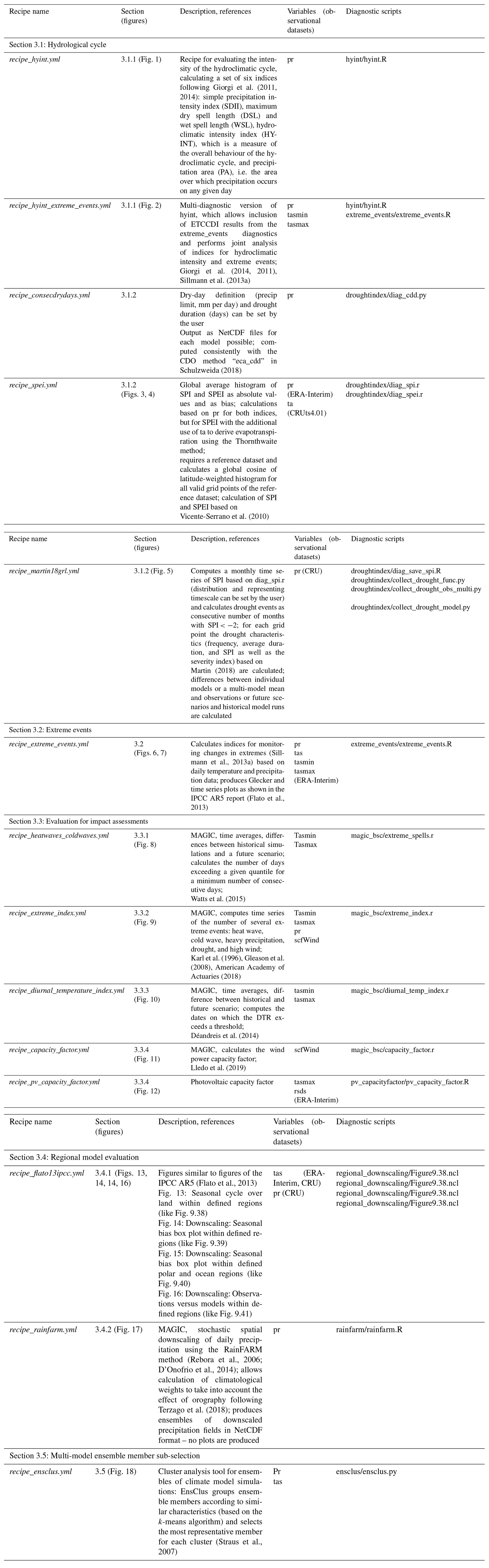
Table 1 Overview of recipes implemented in ESMValTool v2.0 along with the section in which they are described, a brief description, the variables used, and the diagnostic scripts included. For further details, we refer to the GitHub repository and documentation at https://docs.esmvaltool.org/ (last access: 1 June 2021).

This paper is organized as follows: Sect. 2 describes the model and observation data used. Section 3 presents the ESMValTool recipes for the analyses of hydroclimatic intensity, droughts, extreme events, model impact evaluation, multi-model ensemble member sub-selection, and regional model evaluation. It also describes use of the ESMValTool as a post-processing tool for further downscaling applications. Section 4 closes with a summary.

2 Models and observations

ESMValTool v2.0 was developed particularly for the analysis of CMIP data (Righi et al., 2020). This work mainly presents results based on the well-established CMIP5 model ensemble, but other model output and observational data, e.g. provided by observations for the Model Intercomparison Project (obs4MIPs; Teixeira et al., 2014; Waliser et al., 2020), can also be analysed. As in version v1.0 (Eyring et al., 2016), ESMValTool v2.0 expects input data to be in a climate and forecast (CF) metadata-compliant Network Common Data Format (NetCDF) following the Climate Model Output Rewrite (CMOR) standard. The detailed requirements for CMOR can be found in these tables (http://pcmdi.github.io/cmor-site/tables.html, last access: 1 June 2021). For the recipes described here, European Centre for Medium-Range Weather Forecasts (ECMWF) ERA-Interim and Climatic Research Unit (CRU) reanalysis data are used for the evaluation of the model results. Table 1 lists these data in case they are used for a recipe. These datasets should be seen as examples as they can easily be replaced by other reanalysis or observational datasets. Reformatting scripts with downloading instructions are provided with the ESMValTool v2.0 to convert many observational datasets to the CMOR standard. A list of observational datasets available can be found in Righi et al. (2020) and in the user's guide at https://docs.esmvaltool.org/en/latest/input.html#supported-datasets (last access: 1 June 2021), where it is updated for newly included datasets. For ECMWF ERA5 “cmorization on the fly” is implemented, which works on the ERA5 NetCDF data directly and does not require prior reformatting.

3 Overview of recipes included in ESMValTool v2.0

This section describes the new and extended ESMValTool v2.0 recipes for analysis of extreme events and regional model output, as well as for applying ESM output in assessments of the impact of climate change and carrying out model ensemble sub-selection. In ESMValTool v2.0, a recipe is a *.yml file used to define the diagnostics and performance metrics to apply to the simulation output, as well as the datasets and variables used. The ESMValTool is started from the command line using the following, for example.

esmvaltool run esmvaltool/recipes/ examples/recipe_python.yml

Here, esmvaltool/recipes/examples/recipe_python.yml is one possible recipe. Instead of this example, any other recipe provided with the ESMValTool or created by the user can be used. For more detailed instructions on how to run the tool and modify or create recipes, see the documentation at https://docs.esmvaltool.org/ (last access: 1 June 2021).

In the following, the recipes are briefly described and illustrated with example figures using CMIP5 data. All recipes presented in this work are summarized in Table 1, which includes a short description, together with the analysed variables used, the applied diagnostics and their purpose, and the references the diagnostics are based on. Because the online documentation for the ESMValTool v2.0 at https://docs.esmvaltool.org/ (last access: 1 June 2021) was written simultaneously with this paper by the same authors, there is considerable overlap in this non-peer-reviewed document.

Section 3.1 describes recipes for the hydrological cycle, including indices for hydroclimatic intensity and drought detection. In Sect. 3.2 recipes for other extreme events are presented. Recipes for model impact assessment are described in Sect. 3.3 and recipes for regional model evaluation in Sect. 3.4. Section 3.5 presents a recipe for the sub-selection of multi-model ensemble members.

3.1 Hydrological cycle

3.1.1 Hydroclimatic intensity and related indices

The Earth's hydrological cycle is a key element of the climate system with important impacts on society. For example, the intensity and distribution of precipitation determine the abundance or scarcity of fresh water in a certain region. They are also related to the severity of hazardous events such as flooding or droughts. Several studies have shown an acceleration of the hydrological cycle and an intensification of both dry and wet extremes in a warming climate (IPCC, 2013). A simple investigation of total precipitation-related quantities can hide some of the most relevant aspects of the hydrological cycle and its extremes, which can be highlighted through the joint use of the concept of hydroclimatic intensity and related indices (e.g. Giorgi et al., 2014). The hydroclimatic intensity (Giorgi et al., 2011), derived as the product of mean daily precipitation and dry spell length normalized over a reference period, offers a joint view of both dry and wet conditions, allowing for the unique quantification of the response in the intensity of the hydrological cycle in a changing climate. The hyint (hydroclimatic intensity) diagnostic was developed to calculate several indices for hydroclimatic and climate extremes and allow a multi-index evaluation of climate models.

The recipe_hyint.yml calculates six indices for evaluating the global warming response of the hydrological cycle including both wet and dry extremes. The indices are selected according to Giorgi et al. (2014), including the simple precipitation intensity index (SDII), the maximum dry spell length (DSL) and wet spell length (WSL), the hydroclimatic intensity index (HY-INT, calculated as normalized DSL times normalized SDII), which is a measure of the intensity of the hydroclimatic cycle compared to a reference period (Giorgi et al., 2011), and the precipitation area (PA), i.e. the area over which precipitation occurs on any given day (Giorgi et al., 2014). The recipe_hyint_extreme_events.yml can also ingest the 27 temperature- and precipitation-based Expert Team on Climate Change Detection and Indices (ETCCDI) (Zhang et al., 2011) calculated by the recipe_extreme_events.yml to produce a multi-index analysis (see Sect. 3.2 for further details). The diagnostics perform a subsequent analysis calculating time series and trends of the selected indices for predefined continental areas, normalized to a reference period. The linear model (lm) function of R is used to calculate trends. Statistical significance is tested based on a Student's t test under a non-null coefficients hypothesis. Trend coefficients and their statistics, including standard error, p value, and precipitation above the 95th percentile of the reference distribution, are stored. The recipe created several plots, including global and regional maps, time series with spread, trend lines, and summary plots of trend coefficients. Results are stored in NetCDF files, including relevant information such as normalization functions and thresholds, and as figures. Figures 1 and 2 show examples of an analysis performed with the hyint diagnostic. A map of the HY-INT index (Fig. 1) calculated from EC-EARTH model data shows the projected average HY-INT compared to the reference period (1976–2005): hydroclimatic intensity is projected to greatly increase in some regions (e.g. eastern South America, northern Africa, and the Arabian peninsula) and to decrease over other regions (e.g. Antarctica, Greenland, central and north-eastern Asia, central Africa, and western and northern South America), with large areas showing only moderate changes. Trends shown in Fig. 2 exhibit a relatively low inter-model spread for HY-INT. The projected increase in HY-INT seen for all models with values ranging around 10 % per century (also reflected as large geographical patterns) can also be seen in the precipitation intensity (SDI) and heavy precipitation indices (R95), the latter with an increased spread between 10 % and 30 % per century. Precipitation area (PA) is projected to increase by most models, whereas for projected changes in the dry spell length (DSL) and especially in the wet spell length (WSL), models do not agree on the sign of the projected changes, which is also reflected in high geographical variability (not shown).

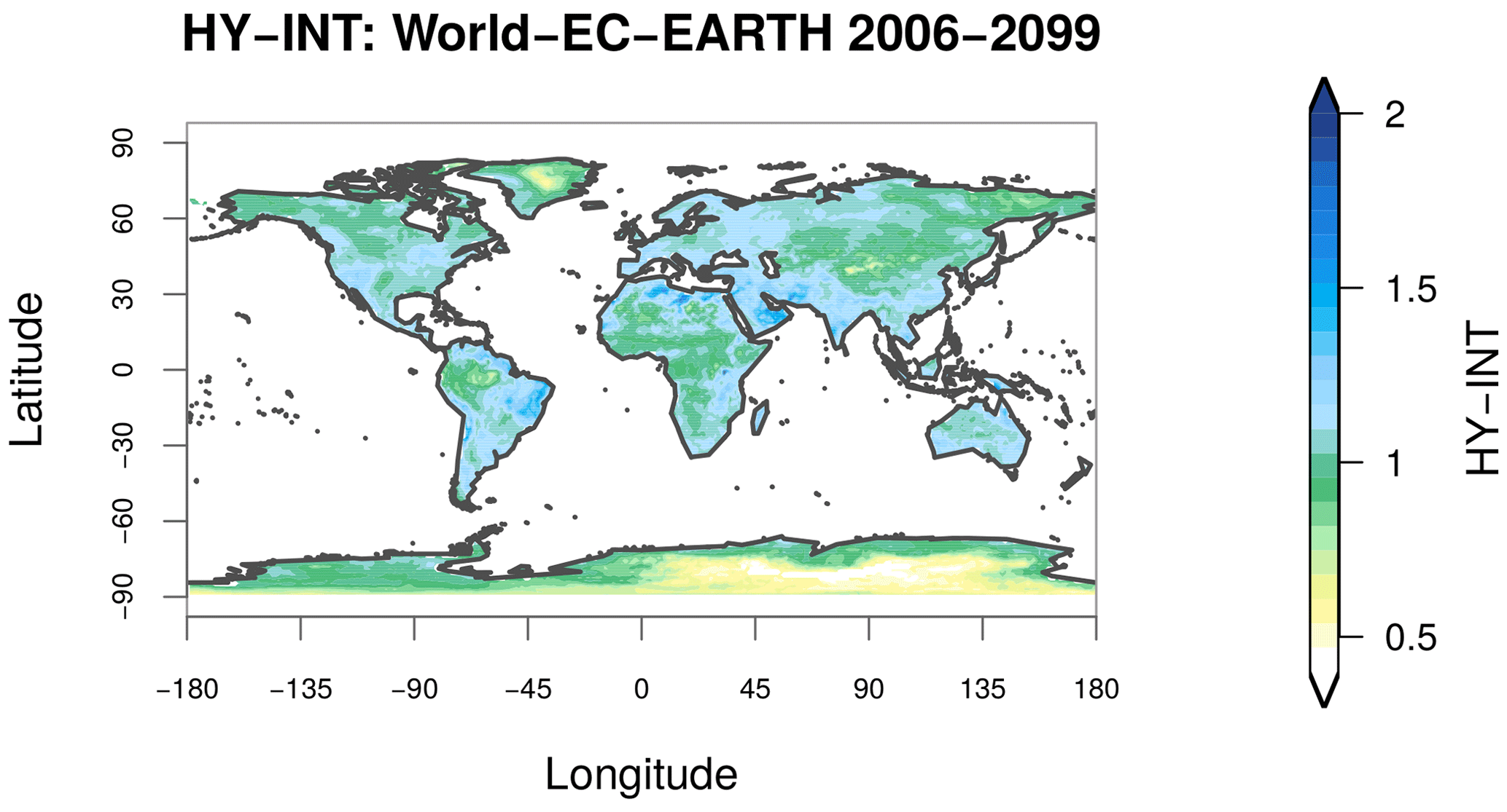
Figure 1 Mean hydroclimatic intensity index (i.e. a combination of precipitation intensity and dry spell length normalized compared to a reference period) over the years 2006–2099, for the EC-EARTH model RCP8.5 projection. The historical years 1976–2005 were used as the reference period. The figure is an example of a large number of different plots which can be produced with recipe_hyint.yml, similar to (Giorgi et al., 2014). For details see Sect. 3.1.1.

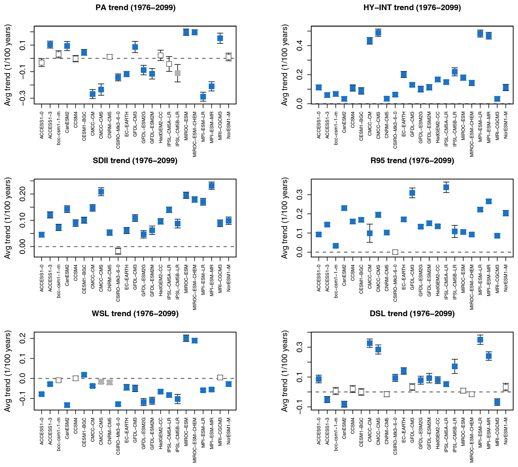
Figure 2 Trend in selected indices for an ensemble of CMIP5 models (historical + RCP8.5 projection) over the time period 1976–2099. The trends are calculated over the latitude band 60^∘ S–60^∘ N. Data were normalized to the historical 1976–2005 period. Indices include the precipitation area (PA), hydroclimatic intensity (HY-INT), precipitation intensity (SDII), heavy precipitation (R95), and wet and dry spell length (WSL and DSL) following Giorgi et al. (2014). Error bars show the geographical variability (standard deviation) within the region and colours the statistical significance of the trend (90 % grey, 95 % blue). This is an example of a large number of different plots which can be produced with recipe_hyint.yml, similar to Giorgi et al. (2014). For details see Sect. 3.1.1.

3.1.2 Droughts

Three main types of droughts can be separated: (i) meteorological, (ii) hydrological, and (iii) agricultural droughts. Any type of drought needs to be defined in the context of local and seasonal characteristics, implying that a drought should be identified as an anomalous condition rather than being based on an absolute threshold.

Meteorological droughts are negative anomalies in precipitation. Depending on the local characteristics, a drought can be defined as an extended period of daily precipitation amounts below a given threshold. The threshold value is defined as the minimum amount of precipitation that is needed to recharge the soil moisture content. This approach requires good knowledge of the local and seasonal characteristics of the soil moisture content. However, it is a useful analysis to investigate climate models' distributions of wet and dry periods, which are indicative of how well suited the model is to couple to hydrological impact models. For example, CMIP5 models have been shown to generally underestimate the number of consecutive dry days (Sillmann et al., 2013b; Cheng et al., 2016). The standardized precipitation index (SPI; McKee et al., 1993) describes local precipitation anomalies and is often used to identify meteorological droughts. The SPI was developed as a replacement for the commonly used Palmer drought indices (Palmer, 1965) to better capture dry and wet anomalies. The SPI is calculated using monthly mean precipitation. Therefore, it does not account for the intensity of single precipitation events and the runoff process. Furthermore, SPI does not account for evaporation from the surface. This implies that one component of the water fluxes at the surface is lacking, which makes SPI incompatible with the concept of hydrological droughts. Evaluation of SPI from CMIP5 models shows large model biases (Ukkola et al., 2018).

A hydrological drought occurs when low water supply effects streams, reservoirs, and groundwater levels and is usually caused by extended periods of meteorological droughts. These hydrological processes are usually not simulated with sufficient detail in climate models. As a consequence, agricultural droughts (i.e. when crops become affected by the hydrological drought) also cannot be simulated properly by the models. Hydrological droughts can, however, be estimated in climate models by accounting for evapotranspiration. This allows for the estimation of surface water retention. The standardized precipitation–evapotranspiration index (SPEI; Vicente-Serrano et al., 2010) has been developed to take into account the effect of evapotranspiration on surface water fluxes. Evapotranspiration is typically not provided by CMIP models, so SPEI often takes other inputs to estimate it, e.g. with the Thornthwaite method based on temperature (Thornthwaite, 1948), the Hargreaves method using the monthly mean of daily minimum and maximum near-surface temperature (tasmin and tasmax) (Hargreaves, 1994), or the Penman–Monteith method using minimum and maximum temperature together with 2 m wind speed (Allen et al., 1994), which is estimated from the surface wind (at 10 m). However, it has been shown that the method used to derive the potential evapotranspiration has little impact on the drought statistics (Burke et al., 2006). In contrast to this finding, Shaw and Riha (2011) conclude that, especially for future scenarios with rising temperatures, potential evapotranspiration based on estimates considering temperature only can lead to an overestimation of SPEI.

In order to assess the performance of drought characteristics in climate models, three diagnostics have been implemented into the ESMValTool (v2.0): consecutive dry days, SPI, and SPEI. The consecutive dry days diagnostic (recipe_consecdrydays.yml) has been implemented consistently with the CDO method “eca_cdd” (Climate Data Operators, Schulzweida, 2018), and the SPI and SPEI diagnostics (recipe_spei.yml) are based on the R package SPEI (https://cran.r-project.org/web/packages/SPEI/SPEI.pdf, last access: 1 June 2021; Vicente-Serrano et al., 2010). The recipe recipe_spei.yml computes the SPI and SPEI quantities for each model and summarizes the statistics of both indices as global averages in categories from “extremely dry” to “extremely wet”; see Figs. 3 and 4. By including an estimate for evapotranspiration, the model biases are reduced, particularly for the overly frequent “moderately wet” category. For SPI (Fig. 3), the bias plot shows a clear underestimation of dry and wet conditions, which are mainly compensated for by overly frequent moderately and extremely wet conditions. For the neutral condition category, the results differ depending on the models, with a tendency towards overly frequent occurrence in most models. For SPEI (Fig. 4) the bias plot indicates overly frequent neutral conditions at the expense of mainly dry and wet conditions. Moderate and extreme wet conditions are overestimated in practically all models, whereas moderately and extremely dry conditions show the opposite behaviour.

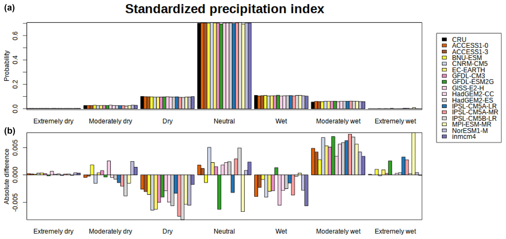
Figure 3 Output from SPI diagnostic in recipe_spei.yml with globally averaged histograms of SPI over land areas, weighted by the cosine of latitude for a selection of CMIP5 models and using gridded observations from CRUts4.01. (a) Absolute values and (b) bias of all models compared to CRUts4.01; for details see Sect. 3.1.2.

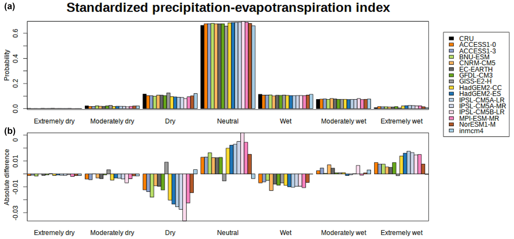
Figure 4 Output from the SPEI diagnostic in recipe_spei.yml with globally averaged histograms of SPEI over land areas, weighted by the cosine of latitude for a selection of CMIP5 models and using gridded observations from CRUts4.01. (a) Absolute values and (b) bias of all models compared to CRUts4.01; for details see Sect. 3.1.2.

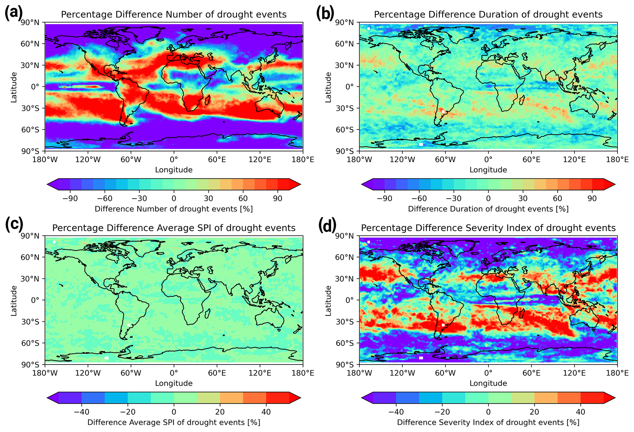
Figure 5 Difference in number (a), duration (b), average SPI (c), and severity index (d) of drought events between the RCP8.5 (2050–2100) and historic (1950 to 2000) multi-model mean of 15 CMIP5 models. Here, a drought event is defined as any number of consecutive months with an SPI $<-\mathrm{2}$. For the SPI calculation a gamma distribution and a representative timescale of 6 months are used. The figure is similar to Fig. 3a–d of Martin (2018) and produced with recipe_martin18grl.yml; for details see Sect. 3.1.2.

Using the SPI calculation described above, a recipe analysing drought events (recipe_martin18.yml) has been developed. Following Martin (2018), a drought event is defined as any consecutive number of months with extremely dry conditions (SPI $<-\mathrm{2}$). The characteristics of these events from historical and future scenario model runs (see Fig. 5) as well as from observational data are then compared. The characteristics investigated are frequency, length, average SPI, and the severity index following Peters (2014), which is a measure combining the length and the SPI value of a drought. Figure 5 shows an increase in the number of drought events, the severity index, and to a lesser extent the duration of drought events in the RCP8.5 scenario compared to the historical model runs, especially in subtropical areas. The results support the finding that regions with already dry conditions are much more likely to show a higher number of drought events for the RCP8.5 scenario, known as the “dry gets drier and the wet gets wetter” (DDWW) paradigm (Greve et al., 2014).

3.2 Extreme events

Changes in climate extremes are of utmost concern for society as the consequences of climate change will be strongly manifested in the severe impacts of extreme events, such as heat waves and extreme precipitation, on human and natural systems. Some confidence in future projections of extreme events can be gained by evaluating the models' performance in simulating historical events against observational data and reanalysis datasets. The 27 core climate extremes indices defined by the ETCCDI (Zhang et al., 2011) are able to capture different characteristics of temperature and precipitation extremes and are suitable for monitoring observed climate extremes, model evaluation, and analysis of changes in climate extremes in future climate projections (e.g. Sillmann et al., 2013a, b; Donat et al., 2013). To calculate these indices, daily values of total precipitation (pr), daily mean near-surface air temperature (tas), daily minimum near-surface air temperature (tasmin), and daily maximum near-surface air temperature (tasmax) are required.

The recipe_extreme_events.yml calculates climate extremes indices and produces diagnostic figures for comparing model and observational extremes indices as presented in IPCC AR5 chapter 9 (Flato et al., 2013) and Sillmann et al. (2013a).

The index computation is performed according to Zhang et al. (2005b). The indices are calculated from CMIP models as well as gridded observational and reanalysis data. Calculating the indices can take several hours to days depending on the number of models and observations, the length of the time periods analysed, and the spatial resolution of the datasets as well as the computational resources. If possible, it is recommended to run this processing step on a parallel computing system, taking advantage of the ESMValTool task-based parallelization feature (Righi et al., 2020).

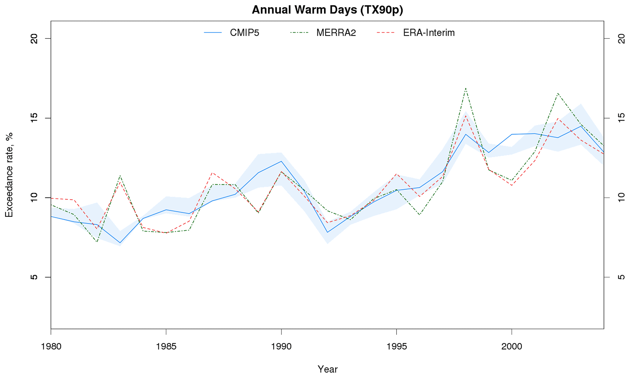
Figure 6 Time series plot of the annual percentage of days when the daily maximum temperature is higher than the 90th percentile for the respective calendar day. Percentile thresholds are calculated following Zhang et al. (2005b) for the base period 1980–2004. The shading indicates the interquartile ensemble spread (range between the 25th and 75th quantiles). The CMIP5 ensemble mean (blue line, five models in this example) averaged over all land grid boxes is compared with the reanalysis datasets MERRA-2 (green dashed line) and ERA-Interim (red dashed line). Similar to Fig. 9.37 e of IPCC AR5 (Flato et al., 2013) and produced with recipe_extreme_events.yml; for details see Sect. 3.2.

There are two types of diagnostic plots that can be produced together and that reproduce the analysis shown in Fig. 9.37 of IPCC AR5 (Flato et al., 2013) for a given reanalysis and model dataset. The first one (see Fig. 6) shows time series providing a temporal comparison between the mean and spread (interquartile range) of the CMIP5 model ensemble and the individual observations for a single index. In Fig. 6, the agreement in trends between the CMIP5 models and reanalyses can be captured very well due to the construction of the percentile-threshold-based indices. Deviations from the nominal level of 10 % outside the base period are mainly due to differences in the estimated trends in tasmin and tasmax of the individual models compared to the respective reanalysis dataset. In Sillmann et al. (2014) an alternative approach is described to evaluate percentile-threshold-based indices accounting for potential model biases in the mean.

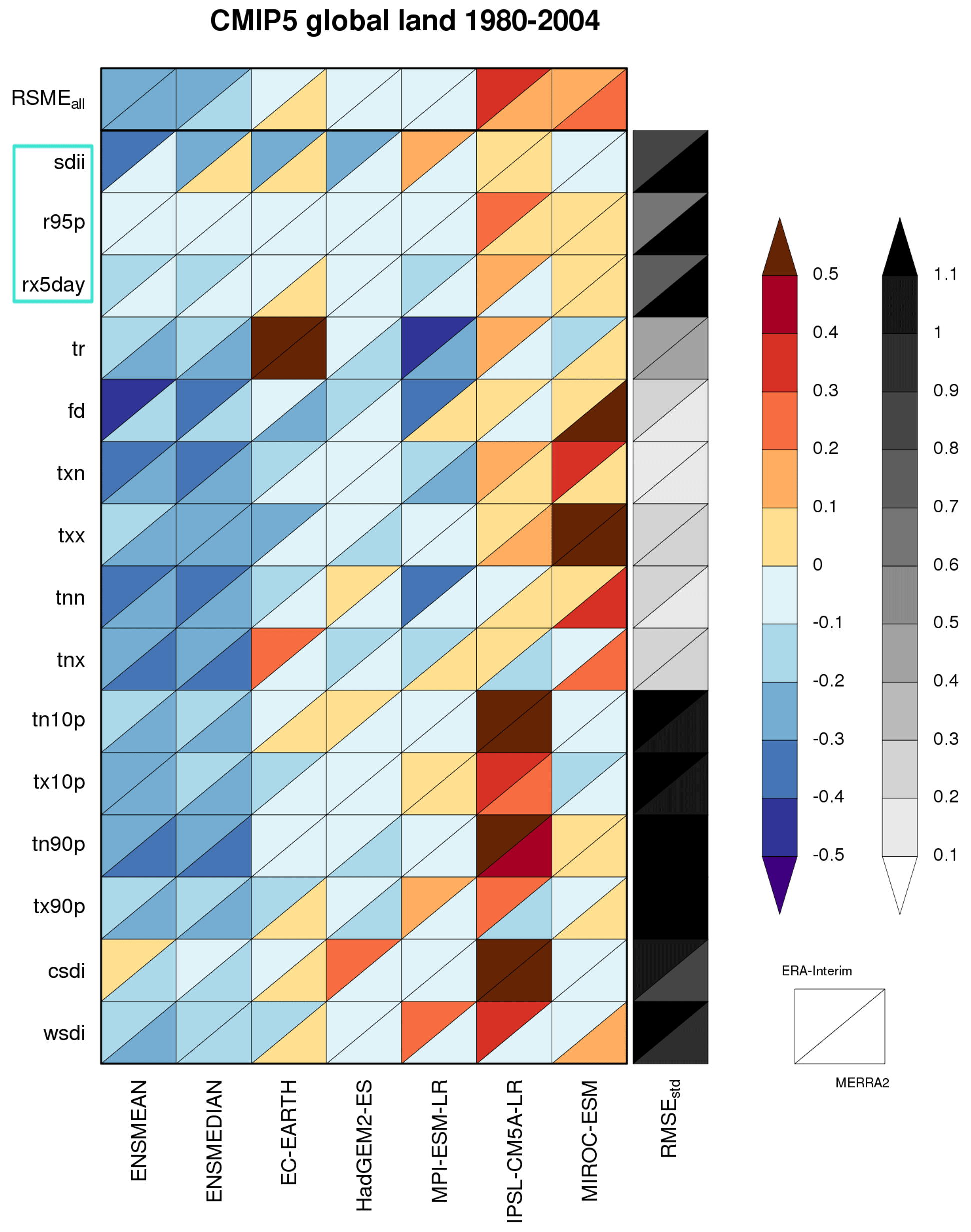
Figure 7 “Portrait” diagram showing relative spatially averaged root mean square error (RMSE) in the 1980–2004 climatologies of 12 temperature and 3 precipitation indices (marked with a blue rectangle) simulated by CMIP5 models (5 in this example along the x axis) with respect to the two reanalyses ERA-Interim (upper triangle) and MERRA-2 (lower triangle). The RMSEs are spatially averaged over all land grid points. The top row (RMSE_all) indicates the mean relative RMSE across all indices for the CMIP5 ensemble mean (first column) and median (second column) as well as each model individually. Blue (red) indicates that a model performs better (worse) than the median of all model results when compared to the respective reanalysis dataset. The grey shaded column at the right-hand side indicates the median RMSE normalized by the spatial standard deviation of the index climatology in the reanalyses (RMSE_std). The root mean square error is shown in greyscale on the right. See Sillmann et al. (2013a) for details. Similar to Fig. 9.37a of the IPCC AR5 report (Flato et al., 2013) and produced with recipe_extreme_events.yml; for details see Sect. 3.2.

The second diagnostic plot (Fig. 7) shows performance metrics in a “portrait diagram”, which compares multiple models with up to four different observations for multiple indices. The root mean square error (RMSE) between each model and each observational or reanalysis dataset is used as a measure for model performance. Figure 7 shows that the magnitude of median RMSE normalized by the spatial standard deviation of the index climatology in the reanalyses (RMSEstd) is generally larger for precipitation indices than for the absolute and percentile-threshold indices based on temperature, with the exception of csdi and wsdi. For the temperature-based percentile-threshold indices (i.e. tx90p, tx10p, tn90p, and tn10p), the models generally perform well (except IPSL-CM5A-LR) due to their construction. This results in good agreement for the ensemble mean and medians compared to reanalysis data, whereas the root mean square error is too large as it is dominated by the outlier model (IPSL-CM5A-LR).

Indices of climate extremes are a natural extension of those for the hydrological cycle discussed in Sect. 3.1, and effort was made to make them available within the same analysis tool. As mentioned before, the ETCCDI computed by recipe_extreme_events.yml can be further processed by the recipe recipe_hyint_extreme_events.yml. Analogous to the recipe_hyint.yml (see also Sect. 3.1.1), it computes maps and box-averaged time series for pre-selected continental or user-defined regions, computing trends and performing significance testing over the complete set of 6+27 indices. Depending on the specific objective, the user can select the needed subset of indices. Significance testing is performed with a Student's t test on the non-null coefficients hypothesis, and trend coefficients are stored together with their statistics. The recipe produces a variety of plot types for the indices, including maps and time series with their spread, trends, and summary plots of trend coefficients.

3.3 Impacts of climate change

3.3.1 Heat wave and cold wave duration

Heat waves are expected to become one of the greatest threats to human health in the 21st century due to projected increases in both frequency and severity (IPCC, 2013; Ouzeau et al., 2016), while the duration, intensity, and frequency of cold waves are expected to decrease. It is not clear yet, however, what the impact of changes in heat waves and cold waves on related mortality will be, since mortality due to heat waves and cold waves inferred from historical simulations is typically overestimated. This is partly due to challenges in the correct simulation of extremes (Wang et al., 2016). In the case of heat waves in particular, models have been shown to contain biases in the 90th and 10th percentiles over the historical period (Pereira et al., 2017). However, by using a bias adjustment method based on percentiles, climate models are able to produce output which is consistent with events observed during the historical period (Ouzeau et al., 2016).

The diagnostics of the recipe_heatwaves_coldwaves.yml uses the daily maximum or minimum temperatures to estimate the relative change in heat wave and cold wave characteristics in future climates compared to a reference period. The user selects the model, emissions scenario, the region of interest, and the reference as well as the projection periods and the percentile which will be used to compute the threshold for exceedance or non-exceedance from the reference period (a separate threshold is computed for each day of the selected season and grid point using the quantile bootstrapping method described in Zhang et al., 2005b). Further options which can be selected include whether to compute the frequency of exceedances or non-exceedances of extremely high or extremely low temperature events, respectively. Additionally, the minimum duration of an event to be classified as a heat wave or cold wave and the season of interest can be set. The diagnostic calculates the number of consecutive days over which temperature exceeds or does not exceed the given threshold in future climate projections. The result is presented as annual time series of the total number of heat wave or cold wave days for the selected season at each grid point, and the average number of these days for the selected season in the future climate projections is calculated; see Fig. 8.

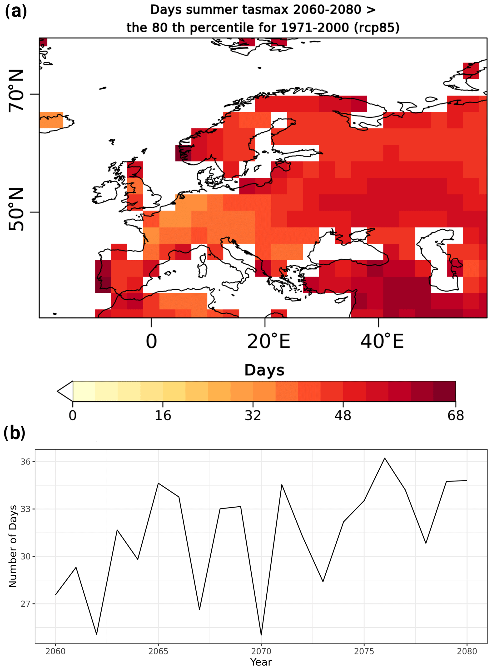
Figure 8 (a) Average annual number of summer days during the time period 2060–2080 when the daily maximum near-surface air temperature exceeds the 80th percentile of the 1971–2000 reference period. The minimum duration of a heat wave event can be chosen in the recipe and is set to 5 d here. (b) Mean annual number of summer days when the daily maximum near-surface air temperature exceeds the 80th percentile of the 1971–2000 reference period averaged over the region shown in (a). Results shown are for the RCP8.5 scenario simulated by BCC-CSM1-1 (see Sect. 3.3.1 for details on recipe_heatwaves_coldwaves.yml).

3.3.2 Combined climate extreme index

High mortality rates, increases in hospital admissions, and major economic losses are often associated with extreme events (Meehl et al., 2000; Zhang et al., 2011; Fouillet et al., 2006; Whitman et al., 1997). This emphasizes the need for monitoring and forecasting extreme events, in particular since some studies suggest that extremes are increasing in both frequency and severity with increasing anthropogenic greenhouse gases (Alexander et al., 2006; Donat et al., 2013).

The recipe recipe_extreme_index.yml allows a user to compute the combined climate extreme index, which is defined as a combination of different extreme values linked to precipitation, surface temperature, and surface wind speed. This index is similar to the climate extremes index (CEI; Karl et al., 1996), the modified CEI (mCEI; Gleason et al., 2008), and the actuaries climate index (ACI; American Academy of Actuaries, 2018). In recipe_extreme_index.yml, the user defines the area, the reference period, the period of interest, and the weights assigned for each individual component of the index. The weights allow the user to put emphasis on the extremes that are more relevant to them and/or completely exclude non-relevant ones. Temperature and precipitation extremes are defined in a similar fashion as in Donat et al. (2013) and are part of the larger set of extreme indices compiled by the ETCCDI (Zhang et al., 2011). The different components of the multi-metric index are the following:

• weight_t90p representing the number of days when the maximum temperature exceeds the 90th percentile,

• weight_t10p representing the number of days when the minimum temperature falls below the 10th percentile,

• weight_Wx representing the number of days when wind power (third power of wind speed) exceeds the 90th percentile,

• weight_cdd representing the maximum length of a dry spell (defined as the maximum number of consecutive days when the daily precipitation is below 1 mm), and

• weight_rx5day representing the maximum precipitation accumulated during 5 consecutive days.

The thresholds are computed for each day in a season using a 5 d running window as described in Zhang et al. (2005a). For the calculation of the index a user-defined reference period is used for normalization and computation of the threshold corresponding to the selected metric. This recipe creates a plot containing the time average of the components listed above for the period of interest (Fig. 9a–e). The recipe also computes the area-weighted average of those components and combines them into a single index using the weights and the running mean (running_mean parameter) defined by the user. The output of the recipe consists of a NetCDF file of the area-weighted and multi-model multi-metric index and a plot of the time series of that index over the selected period.

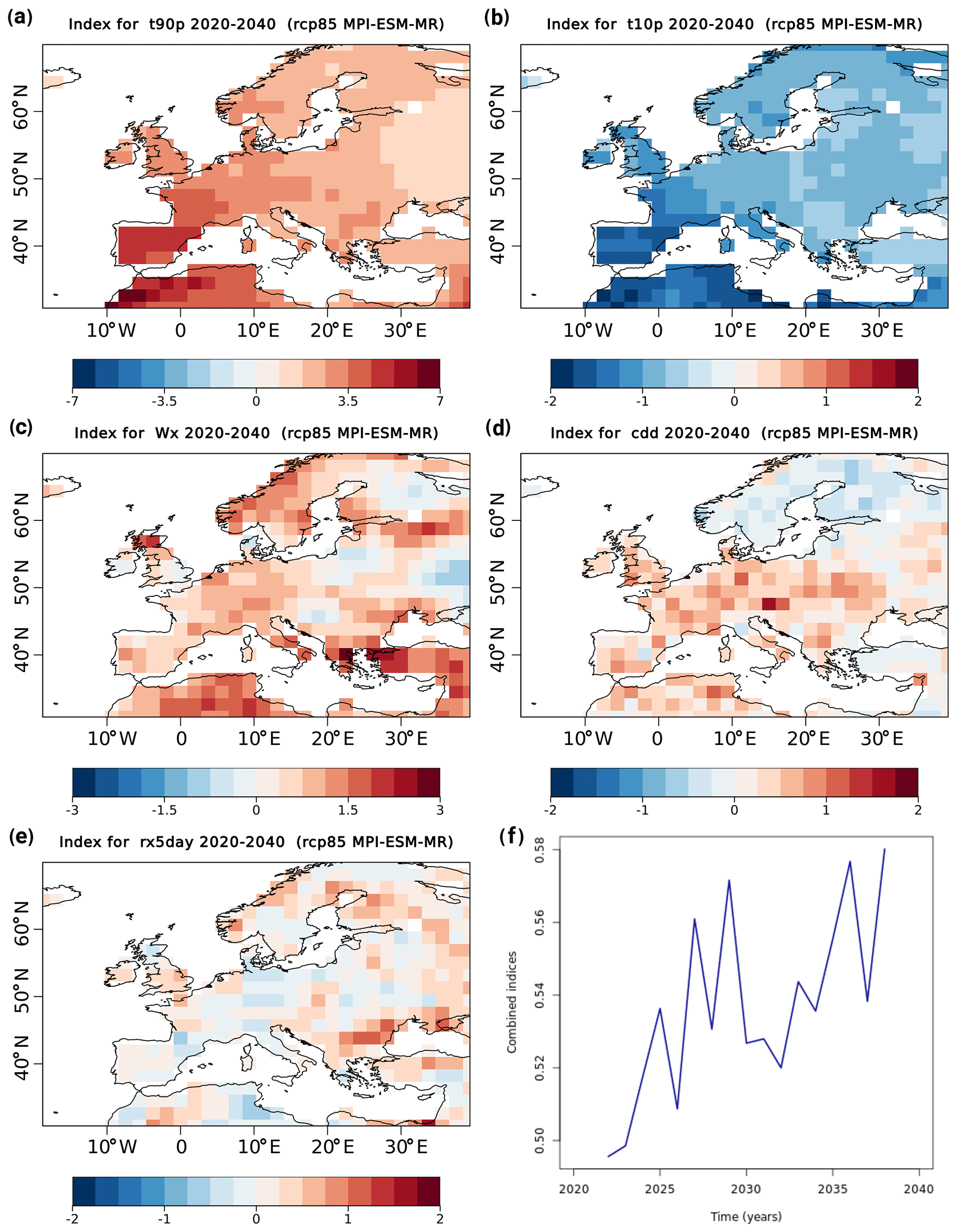
Figure 9 (a–e) Average change in each of the components of the combined climate extreme index for the time period 2020–2040 compared to the 1971–2000 reference period: (a) upper temperature percentile, (b) lower temperature percentile, (c) wind, (d) drought, (e) maximum precipitation. Panel (f) shows a time series for the combined index for 2020–2040. The results are shown for the RCP8.5 scenario simulated by MPI-ESM-MR (see Sect. 3.3.2 for details on recipe_extreme_index.yml).

3.3.3 Daily temperature range variation

The daily temperature range (DTR) corresponds to the difference between the minimum and maximum temperature within a period of 24 h at a given location. The usefulness of the global average DTR has been demonstrated using both observations and climate model simulations (Braganza et al., 2004). Changes in the mean and variability of the DTR have been shown to have a wide range of impacts on society, for example on the transmission of diseases (Lambrechts et al., 2011; Paaijmans et al., 2010) and energy consumption (Déandreis et al., 2014).

In the energy sector, a vulnerability indicator based on the DTR has been defined to identify locations which may experience increased diurnal temperature variations in the future (Déandreis et al., 2014). Increased diurnal temperature variations put additional stress on the operational management of urban heating systems. A measure for increased diurnal temperature variations is defined as the DTR exceeding the value of the reference period by 5 K at a given location and for a given day of the year. Projections of this measure are currently subject to large uncertainties as projections of both daily maximum and minimum near-surface temperature (tasmax and tasmin) in future climate projections are highly uncertain.

The recipe recipe_diurnal_temperature_index.yml computes the mean DTR for a given reference period using historical simulations and then the number of days on which the DTR in future climate projections exceeds that of the reference period by 5 K or more. The user can define both the reference and projection periods, as well as the region to be analysed. The output produced by this recipe consists of a four-panel plot showing the maps of the projected mean DTR indicator for each season (see Fig. 10) and a NetCDF file containing the corresponding data.

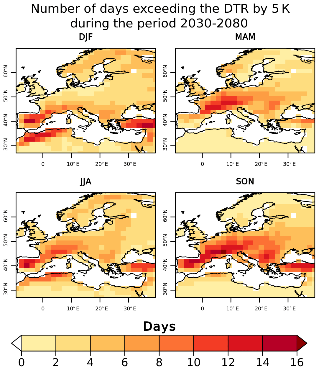
Figure 10 Average number of days per year exceeding the diurnal temperature range (DTR) of the historical period (1961–1990) by 5 K during the period 2030–2080. The example shown is calculated for the RCP8.5 scenario simulated by MPI-ESM-MR (see Sect. 3.3.3 for details on recipe_diurnal_temperature_index.yml).

3.3.4 Capacity factor

The energy sector is the largest contributor to greenhouse gas (GHG) emissions (IPCC, 2014b). Therefore, many countries have adopted mitigation strategies to increase the fraction of energy generated from renewable sources in the forthcoming years. However, renewable energy sources like wind power and solar power rely heavily on atmospheric conditions to produce energy and are therefore exposed to risks from climate variability and long-term change in the case that they lead to detrimental atmospheric conditions. The relationship between wind speed and energy production by wind turbines is highly non-linear because turbines are designed to be efficient for a narrow band of wind speed conditions. Therefore, changes in the wind speed distribution can impact electricity generation and thus the revenues and economic viability of wind farms. The capacity factor is a normalized indicator of the suitability of wind speed conditions to produce electricity, irrespective of the size and number of installed turbines. The factor is provided for wind turbines designed for low, medium, and high wind speed conditions grouped into three different classes (IEC, 2005).

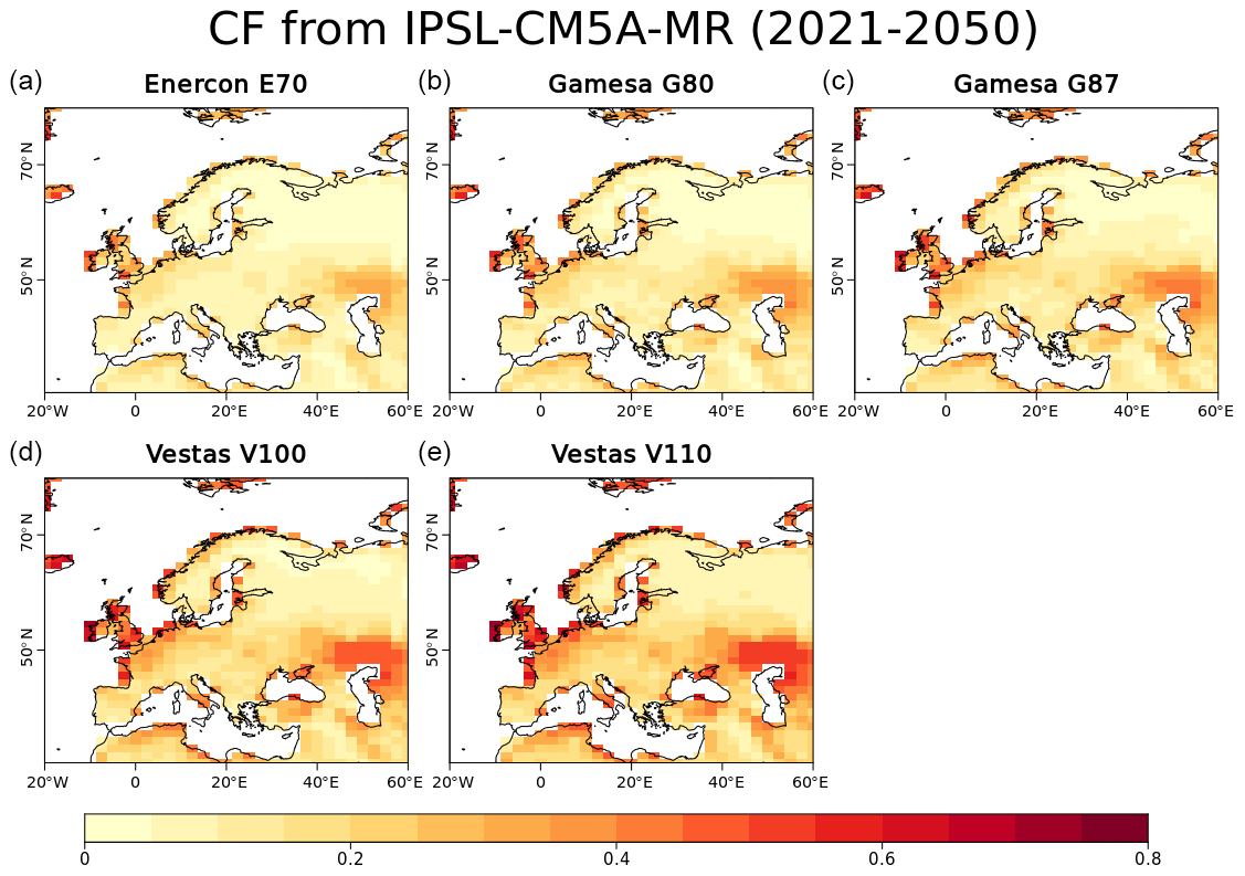
Figure 11 Wind capacity factor for five kinds of wind turbines: Enercon E70 (a), Gamesa G80 (b), Gamesa G87 (c), Vestas V100 (d), and Vestas V110 (e) using the IPSL-CM5A-MR simulation for the RCP8.5 scenario during the period 2021–2050 (see Sect. 3.3.4 for details on recipe_capacity_factor.yml).

The recipe recipe_capacity_factor.yml computes the wind capacity factor for these three wind turbine classes (see Fig. 11) by taking as input the daily instantaneous surface wind speed and extrapolating to the wind speed at 100 m of height as described in (Lledo et al., 2019). The user can select the region, period, and season of interest. The result of the recipe is the capacity factor for each of the three turbine classes saved as a NetCDF file.

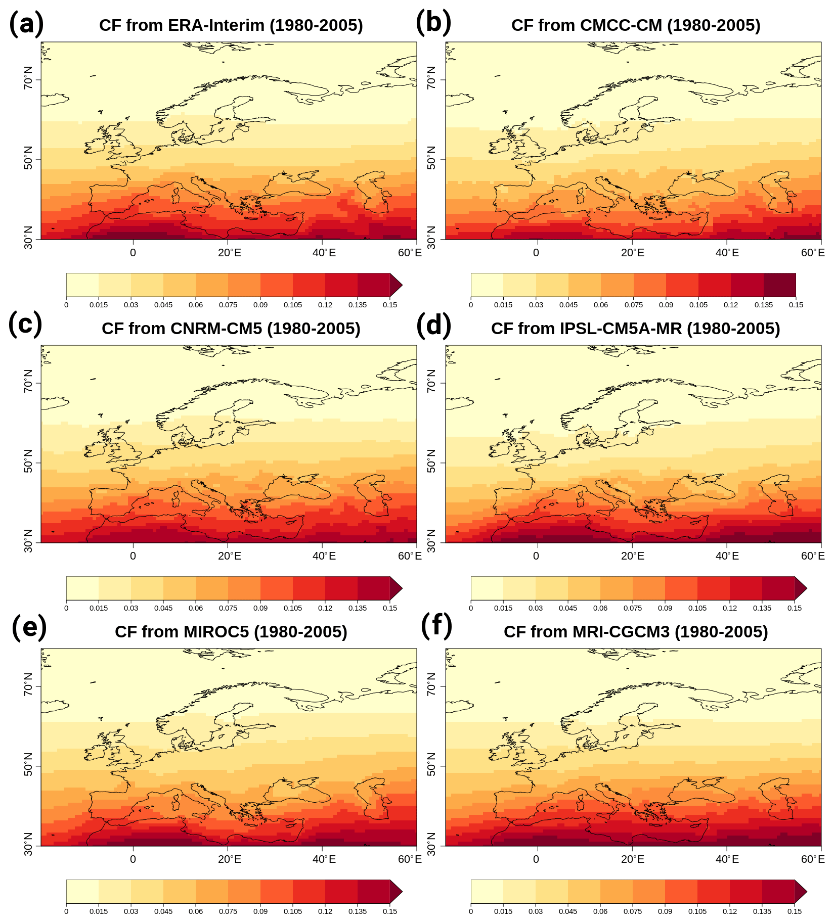
Figure 12 Photovoltaic capacity factor during the DJF period 1980–2005 using ERA-Interim (a), CMCC-CM (b), CNRM-CM5 (c), IPSL-CM5-MR (d), MIROC5 (e), and MRI-CGCM3 (f) (see Sect. 3.3.4 for details on recipe_pv_capacity_factor.yml).

The output of solar photovoltaic (PV) systems depends on the time of the day, season, and weather conditions. The PV capacity factor is a measure of which fraction of the maximum possible energy is produced per grid cell. The solar power generation of a PV system mainly depends on the amount of incoming surface solar radiation but is also influenced by other atmospheric variables that affect the efficiency of PV cells, which decreases as their temperature increases. The recipe_pv_capacity_factor.yml computes the PV capacity factor using the daily incoming surface solar radiation and the surface temperature with a method described in Bett and Thornton (2016). The user can select temporal range, season, and region of interest. An example is shown in Fig. 12 for ERA-Interim and five CMIP5 models.

3.4 Applications for regional scales

3.4.1 Evaluation of global climate models for selected regions

Climate or Earth system models with a fully coupled ocean are important tools to project the future evolution of the climate system in response to anthropogenic forcings, such as the increase in GHG concentrations. Despite their coarse horizontal resolutions (typically of the order of 100 km or less) these models can provide climate information at the regional scale to allow for assessing the impacts of climate change. The ability of these models to simulate regional climate is an important aspect of model evaluation.

The recipe recipe_flato13ipcc.yml includes a subset of diagnostics and figures from the model evaluation chapter of the IPCC AR5 (chapter 9, Flato et al., 2013), which compares surface parameters (such as temperature and precipitation) from models and observations at regional scales.

Figure 13 Difference of the mean seasonal cycle for the surface temperature (tas) between 38 CMIP5 models and ERA-Interim data averaged for 1980–1999 over land in different regions: western North America (WNA), eastern North America (ENA), Central America (CAM), tropical South America (TSA), southern South America (SSA), Europe and the Mediterranean (EUM), North Africa (NAF), central Africa (CAF), southern Africa (SAF), northern Asia (NAS), central Asia (CAS), East Asia (EAS), South Asia (SAS), Southeast Asia (SEA), and Australia (AUS). Similar to Fig. 9.38a of the IPCC AR5 report (Flato et al., 2013) and produced with recipe_flato13ipcc.yml; for details see Sect. 3.4.1.

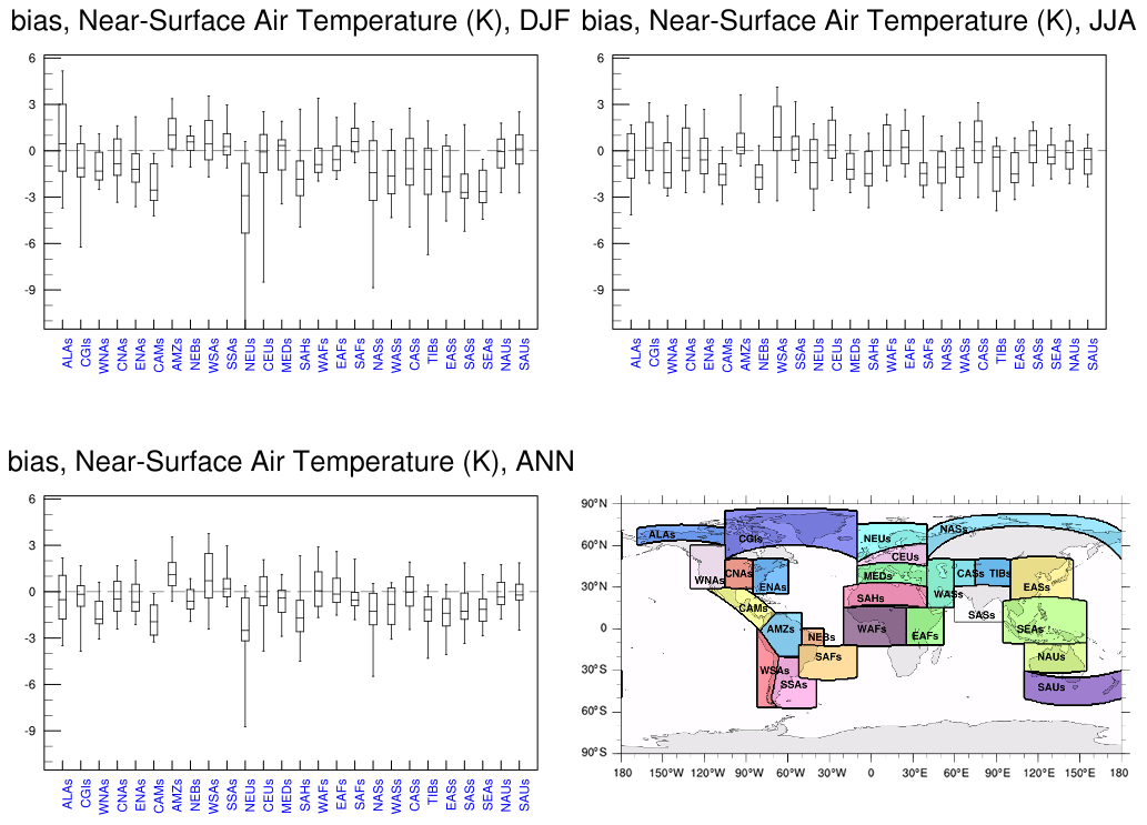
Figure 14 Box-and-whisker plots showing the 5th, 25th, 50th, 75th, and 95th percentiles of the seasonal and annual mean biases for the surface temperature (tas) between 34 CMIP5 models and ERA-Interim data. The regions are as follows: Alaska and NW Canada (ALAs); eastern Canada, Greenland, and Iceland (CGIs); western North America (WNAs); central North America (CNAs); eastern North America (ENAs); Central America and Mexico (CAMs); the Amazon (AMZs); NE Brazil (NEBs); the west coast of South America (WSAs); south-eastern South America (SSAs); northern Europe (NEUs); central Europe (CEUs); southern Europe and the Mediterranean (MEDs); the Sahara (SAHs); western Africa (WAFs); eastern Africa (EAFs); southern Africa (SAFs); northern Asia (NASs); western Asia (WASs); central Asia (CASs); the Tibetan Plateau (TIBs); eastern Asia (EASs); southern Asia (SASs); Southeast Asia (SEAs); northern Australia (NASs); and southern Australia and New Zealand (SAUs). The positions of these regions are shown on the map; they differ from the ones in Fig. 12 and are defined following Seneviratne et al. (2012). Similar to Fig. 9.39a, c, and e of the IPCC AR5 report (Flato et al., 2013) and produced with recipe_flato13ipcc.yml; for details see Sect. 3.4.1.

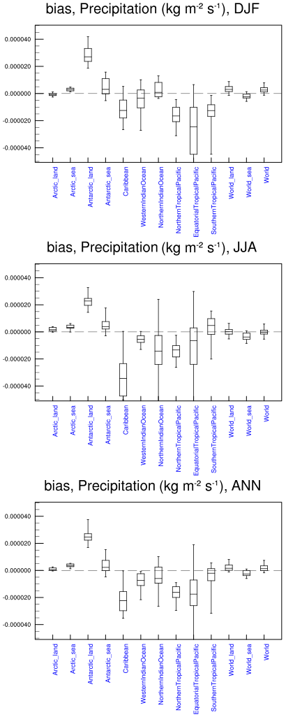
Figure 15 Box-and-whisker plots showing the 5th, 25th, 50th, 75th, and 95th percentiles of the seasonal and annual mean biases for the precipitation (pr) in oceanic and polar regions between 38 CMIP5 models and CRU data. Similar to Fig. 9.40b, d, and f of the IPCC AR5 report (Flato et al., 2013) and produced with recipe_flato13ipcc.yml; for details see Sect. 3.4.1.

The mean seasonal cycle of precipitation and temperature is calculated over land areas within selected regions for individual models, the multi-model mean, and observation and/or reanalysis data (see Fig. 13). Regional biases, including 5th, 25th, 50th, 75th, and 95th percentiles of the biases, in seasonal and annual mean temperature and precipitation are evaluated for several land, polar, and oceanic regions (see Figs. 14 and 15). Diagnostics allow the comparison of the multi-model mean for different projects (i.e. CMIP3, CMIP5) including information on the amplitude of the root mean square error. The regions used in this recipe can be irregular polygons and are defined following the IPCC Special Report on Managing the Risks of Extreme Events and Disasters to Advance Climate Change Adaptation (SREX) land regions (Seneviratne et al., 2012). In addition to the regions described here, the ESMValTool preprocessor can be used to run many diagnostics on distinct regions defined by latitude and longitude limits. We plan to also include regions with more complex boundaries like the CORDEX (Coordinated Regional Downscaling Experiment) regions (Gutowski et al., 2016).

Systematic biases in modelled projections (Boberg and Christensen, 2012) can be investigated by ranking models against observed monthly mean temperature (see Fig. 16).

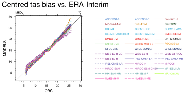
Figure 16 Ranked modelled versus ERA-Interim mean temperature for 38 CMIP5 models in the Mediterranean region (defined as in Fig. 14) for the 1979–2000 period. Similar to Fig. 9.41b of the IPCC AR5 report (Flato et al., 2013) and produced with recipe_flato13ipcc.yml; for details see Sect. 3.4.1.

3.4.2 Stochastic downscaling

The stochastic downscaling recipe is an example of how the ESMValTool (including its pre-processing functionalities) can be used to create a post-processing chain for further downscaling applications, but it is strictly speaking not a diagnostic.

The application of climate model projections and forecasts to impact studies at small scales, such as hydrological modelling or ecological modelling, requires bridging the large gap between the spatial resolution of current global and regional climate models and the scales required for a correct representation of the spatial and temporal structure of precipitation at fine scales as well as of the probability of extreme precipitation events. In the absence of a dynamical, physically based representation, a possible approach is the use of stochastic rainfall downscaling techniques. In particular, the Rainfall Filtered AutoRegressive Model (RainFARM; Rebora et al., 2006; D'Onofrio et al., 2014; Terzago et al., 2018) method is a weather generator which has only one free parameter (which can be derived from large scales) and which requires no further calibration. RainFARM can create ensembles of high-resolution precipitation fields from coarse-scale climate model data. This method also allows quantification of uncertainties and a realistic representation of subgrid-scale variability of precipitation and of precipitation extremes, which is a crucial prerequisite for impact studies in the water sector.

The recipe recipe_rainfarm.yml allows running RainFARM within the ESMValTool. Downscaled output can be produced directly from the climate model results read by the ESMValTool and exploiting its input checking, validation, and pre-processing features. The recipe produces ensembles of downscaled fields (see Fig. 17) over selected regions in NetCDF format, which can then be used by users for further analysis. Notice how the downscaled fields introduce fine-scale precipitation structures while still maintaining on average the original coarse-resolution precipitation. Different stochastic realizations are shown to demonstrate how an ensemble of realizations can be used to reproduce unresolved subgrid variability.

Figure 17 (a) Example of daily accumulated precipitation from the EC-EARTH CMIP5 model on a specific day (artificial date, not a real precipitation event), downscaled using RainFARM from its original resolution (1.125^∘). (b, c) Two stochastic realizations for increasing the spatial resolution by a factor of 8 to 0.14^∘; a fixed spectral slope of s=1.7 was used. The data were produced by recipe_rainfarm.yml, but this plot was not produced by ESMValTool – the recipe output is NetCDF only.

3.5 Multi-model ensemble member sub-selection

Large multi-model ensembles are a way to assess model and scenario uncertainties in future climate projections and other model experiments. However, considering constraints in the availability of computer time and human resources, not all available ensemble members can be included in most detailed climate impact studies associated with a given future scenario. Therefore, despite the importance of using an ensemble that is representative for the region and process of interest covering their full uncertainty range, one or a few ensemble members are often rather subjectively selected depending on, for example, their availability and simplicity in accessing the datasets. Using more specific information about the needs of the impact study as guidance for the selection of simulations, the resulting subset can be better suited for the purpose of climate change impact research. Here, we present an efficient and flexible tool that makes better use of the ensemble by reducing its size while maintaining important ensemble characteristics.

To find an optimal subset of significantly different model projections for a given emission scenario, a clustering algorithm is applied to the multi-model ensemble for data reduction. This technique is already used to characterize the most likely scenarios in an ensemble of weather forecasts (Ferranti and Corti, 2011; Straus et al., 2017). Similar methodologies also based on cluster analysis have been explored to select a subset from an ensemble of climate simulations (Wilcke and Barring, 2016). This approach, applied at a regional level, can also be used to identify the subset of climate model ensemble members that best represent the full range of results for further downscaling applications.

The choice of the ensemble members is made flexible in order to meet the requirements of specific (regional) climate products and can be defined according to region and user needs. The decision of which variables are considered depends on the type and goals of the climate change impact assessment. For example, a study on future hydrological floods would particularly require changes in precipitation extreme quantiles, and a study on the impact of climate change on the exploitation of ski slopes would require information about changes in winter temperatures and precipitation.

EnsClus (recipe recipe_ensclus.yml) is a cluster analysis tool in written in Python for ensembles of climate model simulations. The tool is based on the k-means algorithm with the aim to group ensemble members by similar characteristics and to select the most representative member for each cluster. The user chooses which characteristic is used to group the ensemble members by the clustering: maximum, a given percentile (75 % in the example below), mean, standard deviation, or trend over the period. For each ensemble member this value is computed at each grid point. This results in N latitude–longitude maps, with N representing the number of ensemble members. The anomalies are computed by subtracting the ensemble mean of these maps from each of the individual maps. The anomalies are therefore not computed with respect to time but to the ensemble members. An empirical orthogonal function (EOF) analysis is performed on these anomaly maps. For the EOF analysis, the user can set either how many principal components (PCs) should be calculated or the minimum percentage of the explained variance which should be covered. After reducing dimensionality via EOF analysis, the k-means algorithm is applied using the selected PCs (the number k of clusters needs to be defined prior to the analysis). The output of the recipe is a classification by clusters, i.e. which ensemble member belongs to which cluster and the most representative ensemble member for each cluster, defined by the member being closest to the cluster centroid. Additionally, output of the recipe includes the statistics of clustering: in the PC space, the minimum and the maximum distance between a member in a cluster and the cluster centroid (i.e. the closest and the farthest member), as well as the intra-cluster standard deviation for each cluster (i.e. compactness of the cluster). An example is shown in Fig. 18. The figure shows a clustering based on the 75th percentile of the historical summer (JJA) precipitation rate for 32 CMIP5 models for the period 1900–2005. Based on the principal components explaining 80 % of the variance, three clusters are computed. The green cluster is the most populated with 16 ensemble members. It is mostly characterized by a positive anomaly over central–northern Europe. The red cluster contains 12 ensemble members. It exhibits a negative anomaly centred over southern Europe and in a few cases (e.g. no. 12 and no. 23) extending north. The third cluster (blue) includes only four models. It shows a north–south dipolar precipitation anomaly, with a wetter than average Mediterranean counteracting drier northern Europe. Ensemble members no. 9, no. 26, and no. 19 are the “specimen” of each cluster, i.e. the model simulations that best represent the main features of that cluster. These three ensemble members can eventually be used as representative of all possible outcomes of the multi-model ensemble distribution associated with the 32 CMIP5 historical integrations for the summer precipitation rate 75th percentile over Europe. This reduces the outcomes from 32 to 3 ensemble members. The number of ensemble members of each cluster might provide a measure of the probability of occurrence of each cluster. However, the final results are sensitive to models' bias and to the metric used, as in any selection exercise.

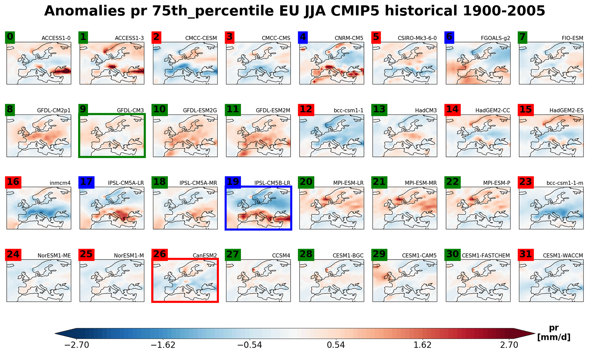
Figure 18 Clustering based on the 75th percentile of the historical summer (JJA) daily precipitation rate for 32 CMIP5 models for the period 1900–2005. The colour of the model number of each ensemble member indicates the cluster to which they belong. The most representative members of each cluster are marked with a coloured border. See Sect. 3.5 for details on recipe_ensclus.yml.

4 Summary

This paper summarizes the recipes available within the ESMValTool v2.0 for the analysis of extreme events, droughts, model impact assessment, sub-selection of multi-model ensemble members (e.g. for downscaling applications), and model evaluation on regional scales. It complements the series of papers that have been published on ESMValTool v2.0 by Righi et al. (2020) describing the technical aspects of ESMValTool v2.0, Eyring et al. (2020) presenting the new large-scale diagnostics that have been included in v2.0 since the first release in 2016 (Eyring et al., 2016), and Lauer et al. (2020) covering emergent constraints and diagnostics for the analysis of future projections from ESMs in CMIP.

For droughts, recipes calculating the consecutive number of dry days, the SPI, and the SPEI have been newly included in ESMValTool v2.0, as has a recipe to analyse the frequency, length, and severity of drought events based on the SPI.

For further analysis of extreme events, climate extreme indices of the Expert Team on Climate Change Detection and Indices (ETCCDI) based on Zhang et al. (2011) have been included. These indices are calculated based on daily total precipitation and the mean, minimum, and maximum of the near-surface air temperature. The indices can then be plotted, used as a measure of model performance, and further processed to calculate index trends and their significance.

For model impact assessments, recipes to analyse heat wave and cold wave duration, diurnal temperature variations, and different extreme indices are included in ESMValTool v2.0. Additional recipes compute capacity factors to analyse the impact of climate change on wind and solar energy production.

For the analysis of ensembles of climate models, ESMValTool v2.0 provides a cluster analysis based on a k-means algorithm whereby the ensemble members are divided into clusters and can be plotted along with the properties of the clusters and the most representative member of each cluster.

ESMValTool v2.0 also includes diagnostics for model evaluation on regional scales. Surface parameters such as temperature and precipitation can be evaluated for regions defined by polygons following the SPEX definitions of land regions. Additionally, the ESMValTool output can be processed further by tools for stochastic downscaling like RainFARM, which is also implemented in v2.0.

Although the recipes here are presented using CMIP5 data, ESMValTool v2.0 can be run to perform the same analysis for CMIP6 data. As an open-source project, the capabilities of the ESMValTool continue to grow, with contributions from the scientific community highly welcome. Users can analyse data using a wealth of existing recipes or join the ESMValTool development team and add new recipes and diagnostics.