the Creative Commons Attribution 4.0 License.
the Creative Commons Attribution 4.0 License.
 | 30 Jul 2020
Earth System Model Evaluation Tool (ESMValTool) v2.0 – an extended set of large-scale diagnostics for quasi-operational and comprehensive evaluation of Earth system models in CMIP
Lisa Bock
Axel Lauer
Mattia Righi
Manuel Schlund
Bouwe Andela
Enrico Arnone
Omar Bellprat
Björn Brötz
Louis-Philippe Caron
Nuno Carvalhais
Irene Cionni
Nicola Cortesi
Bas Crezee
Edouard L. Davin
Paolo Davini
Kevin Debeire
Lee de Mora
Clara Deser
David Docquier
Paul Earnshaw
Carsten Ehbrecht
Bettina K. Gier
Nube Gonzalez-Reviriego
Paul Goodman
Stefan Hagemann
Steven Hardiman
Birgit Hassler
Alasdair Hunter
Christopher Kadow
Stephan Kindermann
Sujan Koirala
Nikolay Koldunov
Quentin Lejeune
Valerio Lembo
Tomas Lovato
Valerio Lucarini
François Massonnet
Benjamin Müller
Amarjiit Pandde
Núria Pérez-Zanón
Adam Phillips
Valeriu Predoi
Joellen Russell
Alistair Sellar
Federico Serva
Tobias Stacke
Ranjini Swaminathan
Verónica Torralba
Javier Vegas-Regidor
Jost von Hardenberg
Katja Weigel
Klaus Zimmermann
The Earth System Model Evaluation Tool (ESMValTool) is a community diagnostics and performance metrics tool designed to improve comprehensive and routine evaluation of Earth system models (ESMs) participating in the Coupled Model Intercomparison Project (CMIP). It has undergone rapid development since the first release in 2016 and is now a well-tested tool that provides end-to-end provenance tracking to ensure reproducibility. It consists of (1) an easy-to-install, well-documented Python package providing the core functionalities (ESMValCore) that performs common preprocessing operations and (2) a diagnostic part that includes tailored diagnostics and performance metrics for specific scientific applications. Here we describe large-scale diagnostics of the second major release of the tool that supports the evaluation of ESMs participating in CMIP Phase 6 (CMIP6). ESMValTool v2.0 includes a large collection of diagnostics and performance metrics for atmospheric, oceanic, and terrestrial variables for the mean state, trends, and variability. ESMValTool v2.0 also successfully reproduces figures from the evaluation and projections chapters of the Intergovernmental Panel on Climate Change (IPCC) Fifth Assessment Report (AR5) and incorporates updates from targeted analysis packages, such as the NCAR Climate Variability Diagnostics Package for the evaluation of modes of variability, the Thermodynamic Diagnostic Tool (TheDiaTo) to evaluate the energetics of the climate system, as well as parts of AutoAssess that contains a mix of top–down performance metrics. The tool has been fully integrated into the Earth System Grid Federation (ESGF) infrastructure at the Deutsches Klimarechenzentrum (DKRZ) to provide evaluation results from CMIP6 model simulations shortly after the output is published to the CMIP archive. A result browser has been implemented that enables advanced monitoring of the evaluation results by a broad user community at much faster timescales than what was possible in CMIP5.


The Intergovernmental Panel on Climate Change (IPCC) Fifth Assessment Report (AR5) concluded that the warming of the climate system is unequivocal and that the human influence on the climate system is clear (IPCC, 2013). Observed increases in greenhouse gases, warming of the atmosphere and ocean, sea ice decline, and sea level rise, in combination with climate model projections of a likely temperature increase between 2.1 and 4.7 ∘C for a doubling of atmospheric CO2 concentration from pre-industrial (1980) levels make it an international priority to improve our understanding of the climate system and to reduce greenhouse gas emissions. This is reflected for example in the Paris Agreement of the United Nations Framework Convention on Climate Change (UNFCCC) 21st session of the Conference of the Parties (COP21; UNFCCC, 2015).
Simulations with climate and Earth system models (ESMs) performed by the major climate modelling centres around the world under common protocols have been coordinated as part of the World Climate Research Programme (WCRP) Coupled Model Intercomparison Project (CMIP) since the early 90s (Eyring et al., 2016a; Meehl et al., 2000, 2007; Taylor et al., 2012). CMIP simulations provide a fundamental source for IPCC Assessment Reports and for improving our understanding of past, present, and future climate change. Standardization of model output in a common format (Juckes et al., 2020) and publication of the CMIP model output on the Earth System Grid Federation (ESGF) facilitates multi-model evaluation and analysis (Balaji et al., 2018; Eyring et al., 2016a; Taylor et al., 2012). This effort is additionally supported by observations for the Model Intercomparison Project (obs4MIPs) which provides the community with access to CMIP-like datasets (in terms of variable definitions, temporal and spatial coordinates, time frequencies, and coverages) of satellite data (Ferraro et al., 2015; Teixeira et al., 2014; Waliser et al., 2019). The availability of observations and models in the same format strongly facilitates model evaluation and analysis.
CMIP is now in its sixth phase (CMIP6, Eyring et al., 2016a) and is confronted with a number of new challenges. More centres are running more versions of more models of increasing complexity. An ongoing demand to resolve more processes requires increasingly higher model resolutions. Accordingly, the data volume of 2 PB in CMIP5 is expected to grow by a factor of 10–20 for CMIP6, resulting in a CMIP6 database of between 20 and 40 PB, depending on model resolution and the number of modelling centres ultimately contributing to the project (Balaji et al., 2018). Archiving, documenting, subsetting, supporting, distributing, and analysing the huge CMIP6 output together with observations challenges the capacity and creativity of the largest data centres and fastest data networks. In addition, the growing dependency on CMIP products by a broad research community and by national and international climate assessments, as well as the increasing desire for operational analysis in support of mitigation and adaptation, means that systems should be set in place that allow for an efficient and comprehensive analysis of the large volume of data from models and observations.
To help achieve this, the Earth System Model Evaluation Tool (ESMValTool) is developed. A first version that was tested on CMIP5 models was released in 2016 (Eyring et al., 2016c). With the release of ESMValTool version 2.0 (v2.0), for the first time in CMIP an evaluation tool is now available that provides evaluation results from CMIP6 simulations as soon as the model output is published to the ESGF (https://cmip-esmvaltool.dkrz.de/, last access: 13 July 2020). This is realized through text files that we refer to as recipes, each calling a certain set of diagnostics and performance metrics to reproduce analyses that have been demonstrated to be of importance in ESM evaluation in previous peer-reviewed papers or assessment reports. ESMValTool is developed as a community diagnostics and performance metrics tool that allows for routine comparison of single or multiple models, either against predecessor versions or against observations. It is developed as a community effort currently involving more than 40 institutes with a rapidly growing developer and user community. Given the level of detailed evaluation diagnostics included in ESMValTool v2.0, several diagnostics are of interest only to the climate modelling community, whereas others, including but not limited to those on global mean temperature or precipitation, will also be valuable for the wider scientific user community. The tool allows for full traceability and provenance of all figures and outputs produced. This includes preservation of the netCDF metadata of the input files including the global attributes. These metadata are also written to the products (netCDF and plots) using the Python package W3C-PROV. Details can be found in the ESMValTool v2.0 technical overview description paper by Righi et al. (2020).
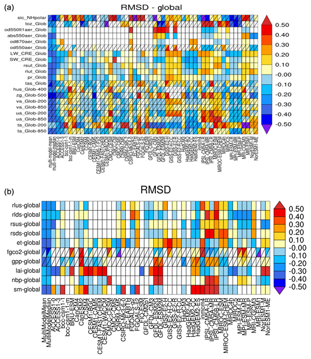
Figure 1Relative space–time root-mean-square deviation (RMSD) calculated from the climatological seasonal cycle of the CMIP5 simulations. The years averaged depend on the years with observational data available. A relative performance is displayed, with blue shading indicating better and red shading indicating worse performance than the median of all model results. Note that the colours would change if models were added or removed. A diagonal split of a grid square shows the relative error with respect to the reference dataset (lower right triangle) and the alternative dataset (upper left triangle). White boxes are used when data are not available for a given model and variable. The performance metrics are shown separately for atmosphere, ocean and sea ice (a), and land (b). Extended from Fig. 9.7 of IPCC WG I AR5 chap. 9 (Flato et al., 2013) and produced with recipe_perfmetrics_CMIP5.yml.; see details in Sect. 3.1.1.
The release of ESMValTool v2.0 is documented in four companion papers: Righi et al. (2020) provide the technical overview of ESMValTool v2.0 and show a schematic representation of the ESMValCore, a Python package that provides the core functionalities, and the diagnostic part (see their Fig. 1). This paper describes recipes of the diagnostic part for the evaluation of large-scale diagnostics. Recipes for extreme events and in support of regional model evaluation are described by Weigel et al. (2020) and recipes for emergent constraints and model weighting by Lauer et al. (2020). In the present paper, the use of the tool is demonstrated by showing example figures for each recipe for either all or a subset of CMIP5 models. Section 2 describes the type of modelling and observational data currently supported by ESMValTool v2.0. In Sect. 3 an overview of the recipes for large-scale diagnostics provided with the ESMValTool v2.0 release is given along with their diagnostics and performance metrics as well as the variables and observations used. Section 4 describes the workflow of routine analysis of CMIP model output alongside the ESGF and the ESMValTool result browser. Section 5 closes with a summary and an outlook.
The open-source release of ESMValTool v2.0 that accompanies this paper is intended to work with CMIP5 and CMIP6 model output and partly also with CMIP3 (although the availability of data for the latter is significantly lower, resulting in a limited number of recipes and diagnostics that can be applied with such data), but the tool is compatible with any arbitrary model output, provided that it is in CF-compliant netCDF format (CF: climate and forecast; http://cfconventions.org/, last access: 13 July 2020) and that the variables and metadata follow the CMOR (Climate Model Output Rewriter, https://pcmdi.github.io/cmor-site/media/pdf/cmor_users_guide.pdf, last access: 13 July 2020) tables and definitions (see, e.g., https://github.com/PCMDI/cmip6-cmor-tables/tree/master/Tables for CMIP6, last access: 13 July 2020). As in ESMValTool v1.0, for the evaluation of the models with observations, we make use of the large observational effort to deliver long-term, high-quality observations from international efforts such as obs4MIPs (Ferraro et al., 2015; Teixeira et al., 2014; Waliser et al., 2019) or observations from the ESA Climate Change Initiative (CCI; Lauer et al., 2017). In addition, observations from other sources and reanalysis data are used in several diagnostics (see Table 3 in Righi et al., 2020). The processing of observational data for use in ESMValTool v2.0 is described in Righi et al. (2020). The observations used by individual recipes and diagnostics are described in Sect. 3 and listed in Table 1. With the broad evaluation of the CMIP models, ESMValTool substantially supports one of CMIP's main goals, which is the comparison of the models with observations (Eyring et al., 2016a, 2019).
In this section, all recipes for large-scale diagnostics that have been newly added in v2.0 since the first release of ESMValTool in 2016 (see Table 1 in Eyring et al., 2016c, for an overview of namelists, now called recipes, included in v1.0) are described. In each subsection, we first scientifically motivate the inclusion of the recipe by reviewing the main systematic biases in current ESMs and their importance and implications. We then give an overview of the recipes that can be used to evaluate such biases along with the diagnostics and performance metrics included and the required variables and corresponding observations that are used in ESMValTool v2.0. For each recipe we provide 1–2 example figures that are applied to either all or a subset of the CMIP5 models. An assessment of CMIP5 or CMIP6 models is, however, not the focus of this paper. Rather, we attempt to illustrate how the recipes contained within ESMValTool v2.0 can facilitate the development and evaluation of climate models in the targeted areas. Therefore, the results of each figure are only briefly described. Table 1 provides a summary of all recipes included in ESMValTool v2.0 along with a short description, information on the quantities and ESMValTool variable names for which the recipe is tested, the corresponding diagnostic scripts and observations. All recipes are included in the ESMValTool repository on GitHub (see Righi et al., 2020, for details) and can be found in the directory: https://github.com/ESMValGroup/ESMValTool/tree/master/esmvaltool/recipes (last access: 13 July 2020).
Table 1Overview of standard recipes implemented in ESMValTool v2.0 along with the section they are described, a brief description, the diagnostic scripts included, as well as the variables and observational datasets used. For further details we refer to the GitHub repository.

We describe recipes separately for integrative measures of model performance (Sect. 3.1) and for the evaluation of processes in the atmosphere (Sect. 3.2), ocean and cryosphere (Sect. 3.3), land (Sect. 3.4), and biogeochemistry (Sect. 3.5). Recipes that reproduce chapters from the evaluation chapter of the IPCC Fifth Assessment Report (Flato et al., 2013) are described within these sections.
3.1 Integrative measures of model performance
3.1.1 Performance metrics for essential climate variables for the atmosphere, ocean, sea ice, and land
Performance metrics are quantitative measures of agreement between a simulated and observed quantity. Various statistical measures can be used to quantify differences between individual models or generations of models and observations. Atmospheric performance metrics were already included in namelist_perfmetrics_CMIP5.nml of ESMValTool v1.0. This recipe has now been extended to include additional atmospheric variables as well as new variables from the ocean, sea ice, and land. Similar to Fig. 9.7 of Flato et al. (2013), Fig. 1 shows the relative space–time root-mean-square deviation (RMSD) for the CMIP5 historical simulations (1980–2005) against a reference observation and, where available, an alternative observational dataset (recipe_perfmetrics_CMIP5.yml). Performance varies across CMIP5 models and variables, with some models comparing better with observations for one variable and another model performing better for a different variable. Except for global average temperatures at 200 hPa (ta_Glob-200), where most but not all models have a systematic bias, the multi-model mean outperforms any individual model. Additional variables can easily be added if observations are available, by providing a custom CMOR table and a Python script to do the calculations in the case of derived variables; see further details in Sect. 4.1.1 of Eyring et al. (2016c). In addition to the performance metrics displayed in Fig. 1, several other quantitative measures of model performance are included in some of the recipes and are described throughout the respective sections of this paper.
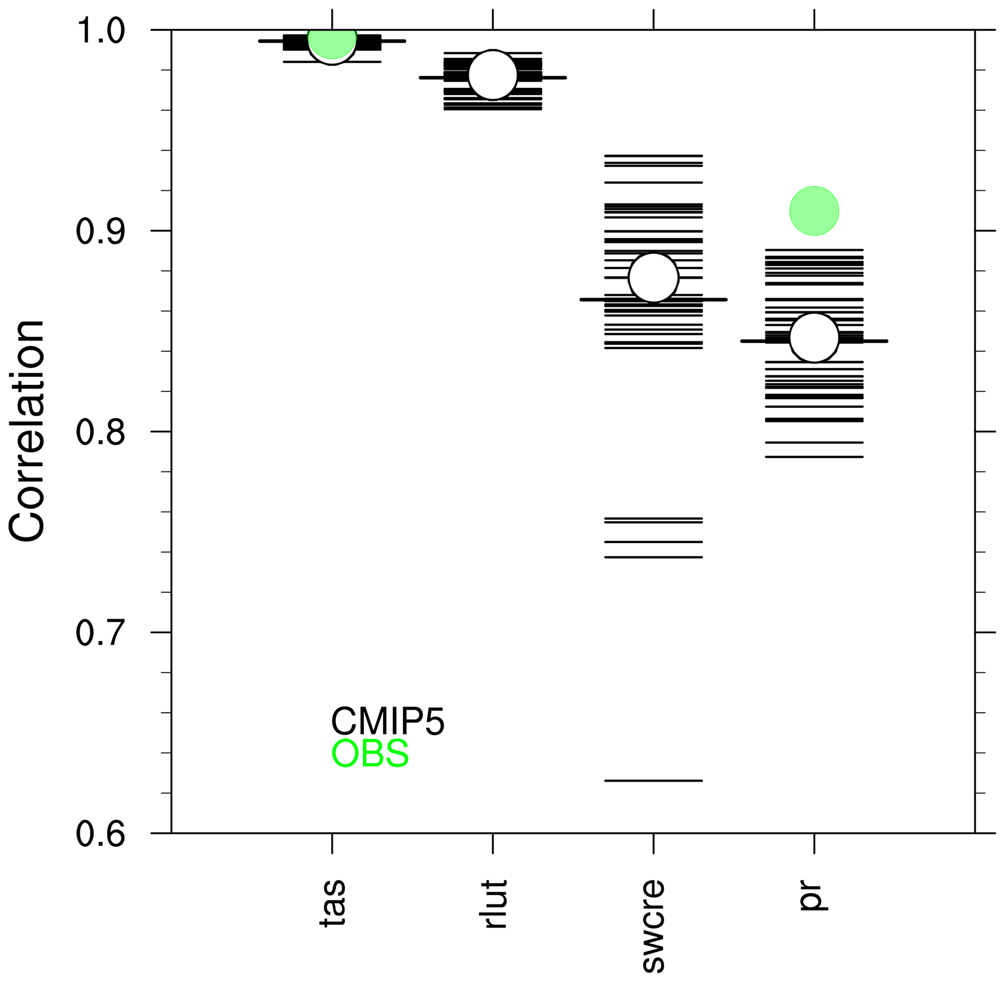
Figure 2Centred pattern correlations for the annual mean climatology over the period 1980–1999 between models and observations. Results for individual CMIP5 models are shown (thin dashes), as well as the ensemble average (longer thick dash) and median (open circle). The correlations are computed between the models and the reference dataset. When an alternate observational dataset is present, its correlation to the reference dataset is also shown (solid green circles). Similar to Fig. 9.6 of IPCC WG I AR5 chap. 9 (Flato et al., 2013) and produced with recipe_flato13ipcc.yml; see details in Sect. 3.1.2.
3.1.2 Centred pattern correlations for different CMIP ensembles
Another example of a performance metric is the pattern correlation between the observed and simulated climatological annual mean spatial patterns. Following Fig. 9.6 of the IPCC AR5 chap. 9 (Flato et al., 2013), a diagnostic for computing and plotting centred pattern correlations for different models and CMIP ensembles has been implemented (Fig. 2) and added to recipe_flato13ipcc.yml. The variables are first regridded to a longitude by latitude grid to avoid favouring a specific model resolution. Regridding is done by the Iris package, which offers different regridding schemes (see https://esmvaltool.readthedocs.io/projects/esmvalcore/en/latest/recipe/preprocessor.html#horizontal-regridding, last access: 13 July 2020). The figure shows both a large model spread as well as a large spread in the correlation depending on the variable, signifying that some aspects of the simulated climate agree better with observations than others. The centred pattern correlations, which measure the similarity of two patterns after removing the global mean, are computed against a reference observation. Should the input models be from different CMIP ensembles, they are grouped by ensemble and each ensemble is plotted side by side for each variable with a different colour. If an alternate model is given, it is shown as a solid green circle. The axis ratio of the plot reacts dynamically to the number of variables (nvar) and ensembles (nensemble) after it surpasses a combined number of nvar×nensemble = 16, and the y axis range is calculated to encompass all values. The centred pattern correlation is a good measure to quantify both the spread in models within a single variable as well as obtaining a quick overview of how well other variables and aspects of the climate on a large scale are reproduced with respect to observations. Furthermore when using several ensembles, the progress made by each ensemble on a variable basis can be seen at a quick glance.
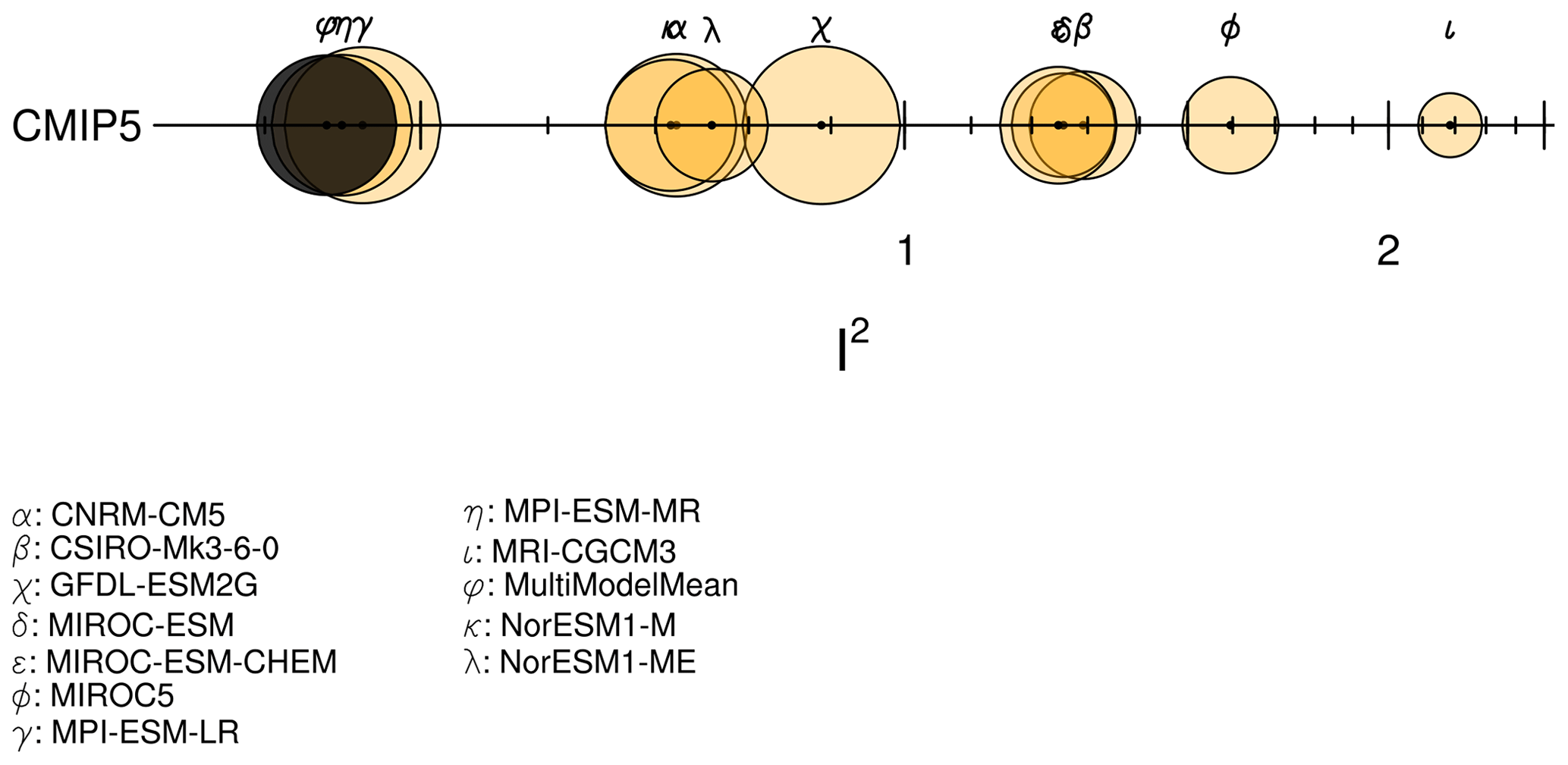
Figure 3Single-model performance index I2 for individual models (orange circles). The size of each circle represents the 95 % confidence interval of the bootstrap ensemble. The black circle indicates the I2 of the CMIP5 multi-model mean. The I2 values vary around 1, with underperforming models having a value greater than 1, while values below 1 represent more accurate models. Similar to Reichler and Kim (2008, Fig. 1) and produced with recipe_smpi.yml; see details in Sect. 3.1.3.
3.1.3 Single-model performance index
Most model performance metrics only display the skill for a specific model and a specific variable at a time, not making an overall index for a model. This works well when only a few variables or models are considered but can result in an overload of information for a multitude of variables and models. Following Reichler and Kim (2008), a single-model performance index (SMPI) has been implemented in recipe_smpi.yml. The SMPI (called “I2”) is based on the comparison of several different climate variables (atmospheric, surface, and oceanic) between climate model simulations and observations or reanalyses and evaluates the time-mean state of climate. For I2 to be determined, the differences between the climatological mean of each model variable and observations at each of the available data grid points are calculated and scaled to the interannual variance from the validating observations. This interannual variability is determined by performing a bootstrapping method (random selection with replacement) for the creation of a large synthetic ensemble of observational climatologies. The results are then scaled to the average error from a reference ensemble of models, and in a final step the mean over all climate variables and one model is calculated. Figure 3 shows the I2 values for each model (orange circles) and the multi-model mean (black circle), with the diameter of each circle representing the range of I2 values encompassed by the 5th and 95th percentiles of the bootstrap ensemble. The SMPI allows for a quick estimation of which models perform the best on average across the sampled variables (see Table 1), and in this case it shows that the common practice of taking the multi-model mean as a best overall model is valid. The I2 values vary around 1, with values greater than 1 for underperforming models and values less than 1 for more accurate models. This diagnostic requires that all models have input for all of the variables considered, as this is the basis for having a meaningful comparison of the resulting I2 values.
3.1.4 AutoAssess
While highly condensed metrics are useful for comparing a large number of models, for the purpose of model development it is important to retain granularity on which aspects of model performance have changed and why. For this reason, many modelling centres have their own suite of metrics which they use to compare candidate model versions against a predecessor. AutoAssess is such a system, developed by the UK Met Office and used in the development of the HadGEM3 and UKESM1 models. The output of AutoAssess contains a mix of top–down metrics evaluating key model output variables (e.g. temperature and precipitation) and bottom–up metrics which assess the realism of model processes and emergent behaviour such as cloud variability and El Niño–Southern Oscillation (ENSO). The output of AutoAssess includes around 300 individual metrics. To facilitate the interpretation of the results, these are grouped into 11 thematic areas, ranging from broad-scale ones such as global tropic circulation and stratospheric mean state and variability, to region- and process-specific, such as monsoon regions and the hydrological cycle.

Figure 4AutoAssess diagnostic for the Quasi-Biennial Oscillation (QBO) showing the time–height plot of zonal mean zonal wind averaged between 5∘ S and 5∘ N for UKESM1-0-LL over the period 1995–2014 in m s−1. Produced with recipe_autoassess_*.yml.; see details in Sect. 3.1.4.
It is planned that all the metrics currently in AutoAssess will be implemented in ESMValTool. At this time, a single assessment area (group of metrics) has been included as a technical demonstration: that for the stratosphere. These metrics have been implemented in a set of recipes named recipe_autoassess_*.yml. They include metrics of the Quasi-Biennial Oscillation (QBO) as a measure of tropical variability in the stratosphere. Zonal mean zonal wind at 30 hPa is used to define metrics for the period and amplitude of the QBO. Figure 4 displays the downward propagation of the QBO for a single model using zonal mean zonal wind averaged between 5∘ S and 5∘ N. Zonal wind anomalies propagate downward from the upper stratosphere. The figure shows that the period of the QBO in the chosen model is about 6 years, significantly longer than the observed period of ∼ 2.3 years. Metrics are also defined for the tropical tropopause cold point (100 hPa, 10∘ S–10∘ N) temperature, and stratospheric water vapour concentrations at entry point (70 hPa, 10∘ S–10∘ N). The cold point temperature is important in determining the entry point humidity, which in turn is important for the accurate simulation of stratospheric chemistry and radiative balance (Hardiman et al., 2015). Other metrics characterize the realism of the stratospheric easterly jet and polar night jet.
3.2 Diagnostics for the evaluation of processes in the atmosphere
3.2.1 Multi-model mean bias for temperature and precipitation
Near-surface air temperature (tas) and precipitation (pr) of ESM simulations are the two variables most commonly requested by users. Often, diagnostics for tas and pr are shown for the multi-model mean of an ensemble. Both of these variables are the end result of numerous interacting processes in the models, making it challenging to understand and improve biases in these quantities. For example, near-surface air temperature biases depend on the models' representation of radiation, convection, clouds, land characteristics, surface fluxes, as well as atmospheric circulation and turbulent transport (Flato et al., 2013), each with their own potential biases that may either augment or oppose one another.
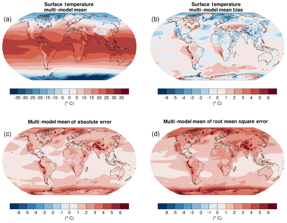
Figure 5Annual-mean surface (2 m) air temperature (∘C) for the period 1980–2005. (a) Multi-model (ensemble) mean constructed with one realization of all available models used in the CMIP5 historical experiment. (b) Multi-model mean bias as the difference between the CMIP5 multi-model mean and the climatology from ECMWF reanalysis of the global atmosphere and surface conditions (ERA)-Interim (Dee et al., 2011). (c) Mean absolute model error with respect to the climatology from ERA-Interim. (d) Mean root-mean-square error of the seasonal cycle with respect to the ERA-Interim. Updated from Fig. 9.2 of IPCC WG I AR5 chap. 9 (Flato et al., 2013) and produced with recipe_flato13ipcc.yml; see details in Sect. 3.2.1.
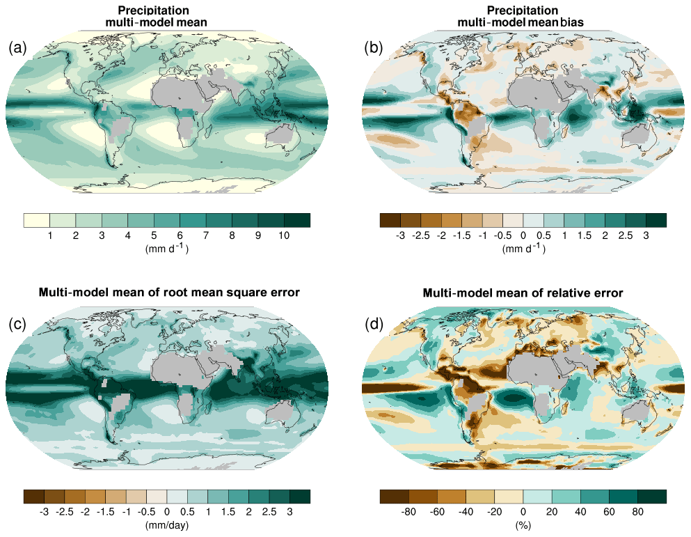
Figure 6Annual-mean precipitation rate (mm d−1) for the period 1980–2005. (a) Multi-model (ensemble) mean constructed with one realization of all available models used in the CMIP5 historical experiment. (b) Multi-model mean bias as the difference between the CMIP5 multi-model mean and the analyses from the Global Precipitation Climatology Project (Adler et al., 2003). (c) Mean root-mean-square error of the seasonal cycle with respect to observations. (d) Mean relative model error with respect to observations. Updated from Fig. 9.4 of IPCC WG I AR5 chap. 9 (Flato et al., 2013) and produced with recipe_flato13ipcc.yml; see details in Sect. 3.2.1.
The diagnostic that calculates the multi-model mean bias compared to a reference dataset is part of recipe_flato13ipcc.yml and reproduces Figs. 9.2 and 9.4 of Flato et al. (2013). We extended the namelist_flato13ipcc.xml of ESMValTool v1.0 by adding the mean root-mean-square error of the seasonal cycle with respect to the reference dataset. The multi-model mean near-surface temperature agrees with ERA-Interim mostly within ±2 ∘C (Fig. 5). Larger biases can be seen in regions with sharp gradients in temperature, for example in areas with high topography such as the Himalaya, the sea ice edge in the North Atlantic, and over the coastal upwelling regions in the subtropical oceans. Biases in the simulated multi-model mean precipitation compared to Global Precipitation Climatology Project (GPCP; Adler et al., 2003) data include precipitation that is too low along the Equator in the western Pacific and precipitation amounts that are too high in the tropics south of the Equator (Fig. 6). Figure 7 shows observed and simulated time series of the anomalies in annual and global mean surface temperature. The model datasets are subsampled by the HadCRUT4 observational data mask (Morice et al., 2012) and preprocessed as described by Jones et al. (2013). Overall, the models represent the annual global-mean surface temperature increase over the historical period quite well, including the more rapid warming in the second half of the 20th century and the cooling immediately following large volcanic eruptions. The figure reproduces Fig. 9.8 of Flato et al. (2013) and is part of recipe_flato13ipcc.yml.
3.2.2 Precipitation quantile bias
Precipitation is a dominant component of the hydrological cycle and as such a main driver of the climate system and human development. The reliability of climate projections and water resource strategies therefore depends on how well precipitation can be simulated by the models. While CMIP5 models can reproduce the main patterns of mean precipitation (e.g. compared to observational data from GPCP; Adler et al., 2003), they often show shortages and biases under particular conditions. Comparison of precipitation from CMIP5 models and observations shows a general good agreement for mean values at a large scale (Kumar et al., 2013; Liu et al., 2012a). Models, however, have a poor representation of frontal, convective, and mesoscale processes, resulting in substantial biases at a regional scale (Mehran et al., 2014): models tend to overestimate precipitation over complex topography and underestimate it especially over arid or some subcontinental regions as for example northern Eurasia, eastern Russia, and central Australia. Biases are typically stronger at high quantiles of precipitation, making the study of precipitation quantile biases an effective diagnostic for addressing the quality of simulated precipitation.

Figure 7Anomalies in annual and global mean surface temperature of CMIP5 models and HadCRUT4 observations. Yellow shading indicates the reference period (1961–1990); vertical dashed grey lines represent times of major volcanic eruptions. The right bar shows the global mean surface temperature of the reference period. CMIP5 model data are subsampled by the HadCRUT4 observational data mask and processed as described in Jones et al. (2013). All simulations are historical experiments up to and including 2005 and the RCP 4.5 scenario after 2005. Extended from Fig. 9.8 of IPCC WG I AR5 chap. 9 (Flato et al., 2013) and produced with recipe_flato13ipcc.yml; see details in Sect. 3.2.1.

Figure 8Precipitation quantile bias (75% level, unitless) evaluated for an example subset of CMIP5 models over the period 1979–2005 using GPCP-SG v2.3 gridded precipitation as a reference dataset. Similar to Mehran et al. (2014) and produced with recipe_quantilebias.yml. See details in Sect. 3.2.2.
The recipe_quantilebias.yml implements the calculation of the quantile bias to allow for the evaluation of precipitation biases based on a user-defined quantile in models as compared to a reference dataset following Mehran et al. (2014). The quantile bias is defined as the ratio of monthly precipitation amounts in each simulation to that of the reference dataset above a specified threshold t (e.g. the 75th percentile of all the local monthly values). An example is displayed in Fig. 8, where gridded observations from the GPCP project were adopted. A quantile bias equal to 1 indicates no bias in the simulations, whereas a value above (below) 1 corresponds to a model's overestimation (underestimation) of the precipitation amount above the specified threshold t, with respect to that of the reference dataset. An overestimation over Africa for models in the right column and an underestimation crossing central Asia from Siberia to the Arabic peninsula is visible, promptly identifying the best performances or outliers. For example, the HadGEM2-ES model here shows a smaller bias compared to the other models in this subset. The recipe allows the evaluation of the precipitation bias based on a user-defined quantile in models as compared to the reference dataset.
3.2.3 Atmospheric dynamics
Stratosphere–troposphere coupling
The current generation of climate models include the representation of stratospheric processes, as the vertical coupling with the troposphere is important for the representation of weather and climate at the surface (Baldwin and Dunkerton, 2001). Stratosphere-resolving models are able to internally generate realistic annular modes of variability in the extratropical atmosphere (Charlton-Perez et al., 2013) which are, however, too persistent in the troposphere and delayed in the stratosphere compared to reanalysis (Gerber et al., 2010), leading to biases in the simulated impacts on surface conditions.
The recipe recipe_zmnam.yml can be used to evaluate the representation of the Northern Annular Mode (NAM; Wallace, 2000) in climate simulations, using reanalysis datasets as a reference. The calculation is based on the “zonal mean algorithm” of Baldwin and Thompson (2009) and is an alternative to pressure-based or height-dependent methods. This approach provides a robust description of the stratosphere–troposphere coupling on daily timescales, requiring less subjective choices and a reduced amount of input data. Starting from daily mean geopotential height on pressure levels, the leading empirical orthogonal functions (EOFs)/principal components are computed from linearly detrended zonal mean daily anomalies, with the principal component representing the zonal mean NAM index. Missing values, which may occur near the surface level, are filled with a bilinear interpolation procedure. The regression of the monthly mean geopotential height onto this monthly averaged index represents the NAM pattern for each selected pressure level. The outputs of the procedure are the time series (Fig. 9a) and the histogram (not shown) of the zonal-mean NAM index and the regression maps for selected pressure levels (Fig. 9b). The well-known annular pattern, with opposite anomalies between polar and mid-latitudes, can be seen in the regression plot. The user can select the specific datasets (climate model simulation and/or reanalysis) to be evaluated and a subset of pressure levels of interest.
Atmospheric blocking indices
Atmospheric blocking is a recurrent mid-latitude weather pattern identified by a large-amplitude, quasi-stationary, long-lasting, high-pressure anomaly that “blocks” the westerly flow forcing the jet stream to split or meander (Rex, 1950). It is typically initiated by the breaking of a Rossby wave in a region at the exit of the storm track, where it amplifies the underlying stationary ridge (Tibaldi and Molteni, 1990). Blocking occurs more frequently in the Northern Hemisphere cold season, with larger frequencies observed over the Euro-Atlantic and North Pacific sectors. Its lifetime oscillates from a few days up to several weeks (Davini et al., 2012). Atmospheric blocking still represents an open issue for the climate modelling community since state-of-the-art weather and climate models show limited skill in reproducing it (Davini and D'Andrea, 2016; Masato et al., 2013). Models are indeed characterized by large negative bias over the Euro-Atlantic sector, a region where blocking is often at the origin of extreme events, leading to cold spells in winter and heat waves in summer (Coumou and Rahmstorf, 2012; Sillmann et al., 2011).
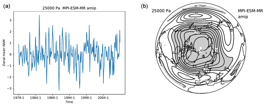
Figure 9The standardized zonal mean NAM index (a, unitless) at 250 hPa for the atmosphere-only CMIP5 simulation of the Max Planck Institute for Meteorology (MPI-ESM-MR) model, and the regression map of the monthly geopotential height on this zonal-mean NAM index (b, in metres). Note the variability on different temporal scales of the index, from monthly to decadal. Similar to Fig. 2 of Baldwin and Thompson (2009) and produced with recipe_zmnam.yml; see details in Sect. 3.2.3.
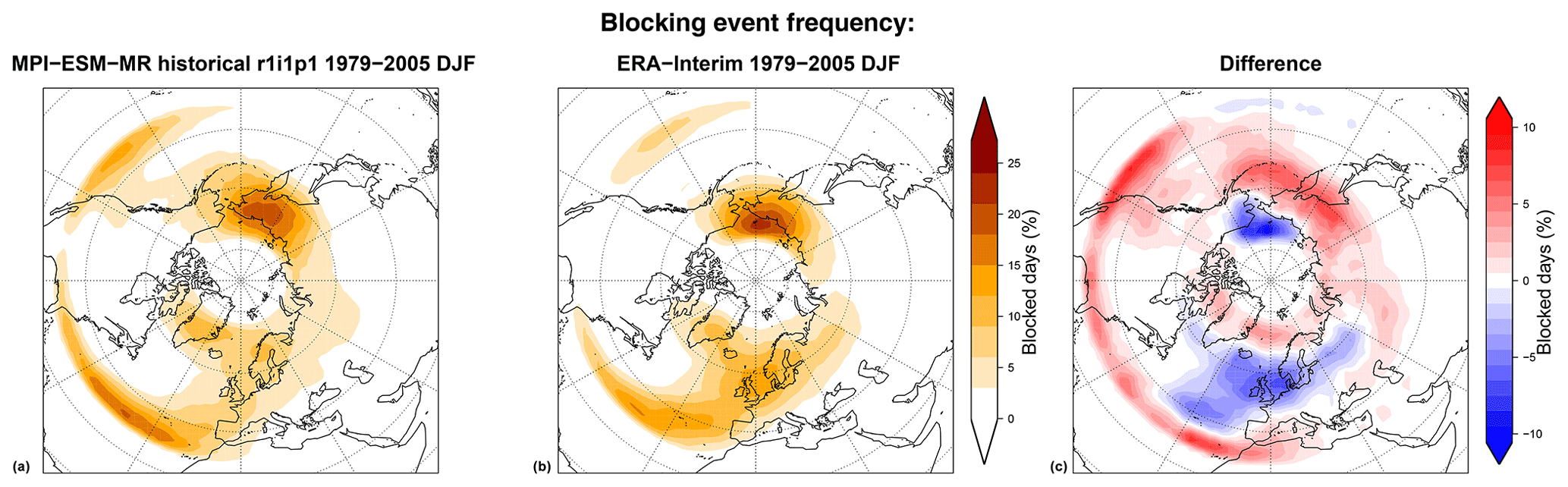
Figure 10Two-dimensional blocking event frequency (percentage of blocked days) following the Davini et al. (2012) index over the 1979–2005 DJF period for (a) the CMIP5 MPI-ESM-MR historical r1i1p1 run, (b) the ERA-Interim Reanalysis, and (c) their differences. Produced with recipe_miles_block.yml; see details in Sect. 3.2.3.2.
Several objective blocking indices have been developed aimed at identifying different aspects of the phenomenon (see Barriopedro et al., 2010, for details). The recipe recipe_miles_block.yml integrates diagnostics from the Mid-Latitude Evaluation System (MiLES) v0.51 (Davini, 2018) tool in order to calculate two different blocking indices based on the reversal of the meridional gradient of daily 500 hPa geopotential height. The first one is a 1-D index, namely the Tibaldi and Molteni (1990) blocking index, here adapted to work with grids. Blocking is defined when the reversal of the meridional gradient of geopotential height at 60∘ N is detected, i.e. when easterly winds are found in the mid-latitudes. The second one is the atmospheric blocking index following Davini et al. (2012). It is a 2-D extension of Tibaldi and Molteni (1990) covering latitudes from 30 up to 75∘ N. The recipe computes both the instantaneous blocking frequencies and the blocking event frequency (which includes both spatial and 5 d minimum temporal constraints). It reports also two intensity indices, namely the Meridional Gradient Index and the Blocking Intensity index, and it evaluates the wave-breaking characteristic associated with blocking (cyclonic or anticyclonic) through the Rossby wave orientation index. A supplementary instantaneous blocking index (named “ExtraBlock”) including an extra condition to filter out low-latitude blocking events is also provided. The recipe compares multiple datasets against a reference one (the default is ERA-Interim) and provides output (in netCDF4 compressed Zip format) as well as figures for the climatology of each diagnostic. An example output is shown in Fig. 10. The Max Planck Institute for Meteorology (MPI-ESM-MR) model shows the well-known underestimation of atmospheric blocking – typical of many climate models – over central Europe, where blocking frequencies are about the half when compared to reanalysis. A slight overestimation of low-latitude blocking and North Pacific blocking can also be seen, while Greenland blocking frequencies show negligible bias.
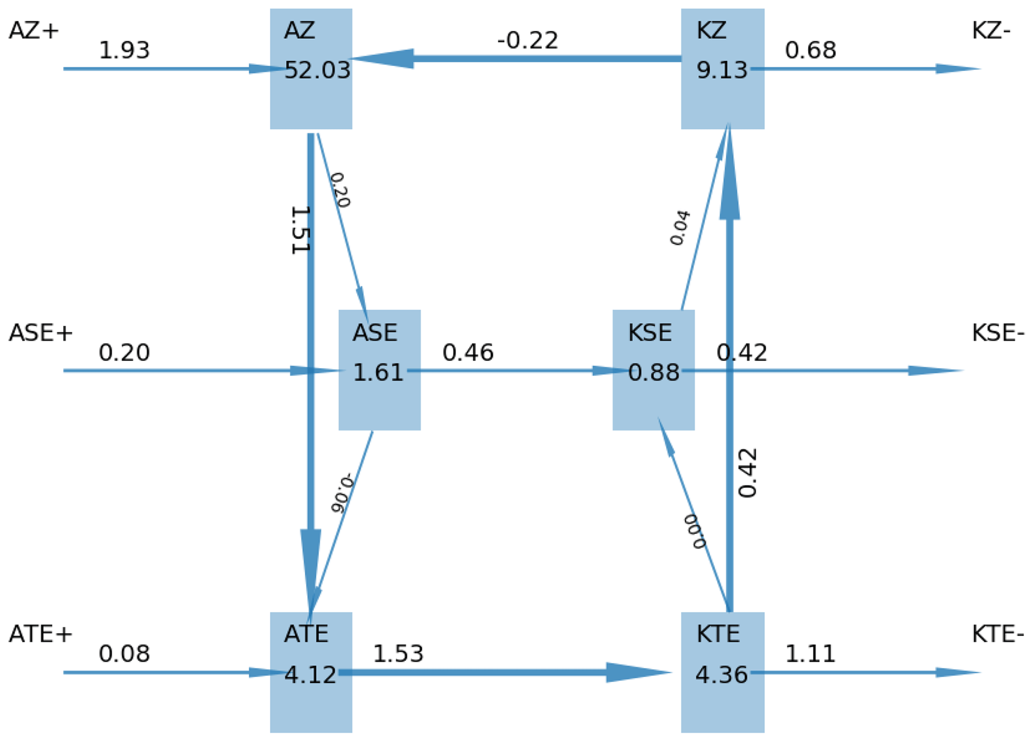
Figure 11A Lorenz energy cycle flux diagram for 1 year of a CMIP5 model pre-industrial control run (cf. Ulbrich and Speth, 1991). “A” stands for available potential energy (APE), “K” for kinetic energy (KE), “Z” for zonal 1115 mean, “S” for stationary eddies, and “T” for transient eddies. The “+” sign indicates source of energy, “−” a sink. For the energy reservoirs, the unit of measure is joules per square metre; for the energy conversion terms, the unit of measure is watts per square metre. Similar to Fig. 5 of Lembo et al. (2019) and produced with recipe_thermodyn_diagtool.yml; see details in Sect. 3.2.4.
3.2.4 Thermodynamics of the climate system
The climate system can be seen as a forced and dissipative non-equilibrium thermodynamic system (Lucarini et al., 2014), converting potential into mechanical energy, and generating entropy via a variety of irreversible processes The atmospheric and oceanic circulation are caused by the inhomogeneous absorption of solar radiation, and, all in all, they act in such a way as to reduce the temperature gradients across the climate system. At steady state, assuming stationarity, the long-term global energy input and output should balance. Previous studies have shown that this is essentially not the case, and most of the models are affected by non-negligible energy drift (Lucarini et al., 2011; Mauritsen et al., 2012). This severely impacts the prediction capability of state-of-the-art models, given that most of the energy imbalance is known to be taken up by oceans (Exarchou et al., 2015). Global energy biases are also associated with inconsistent thermodynamic treatment of processes taking place in the atmosphere, such as the dissipation of kinetic energy (Lucarini et al., 2011) and the water mass balance inside the hydrological cycle (Liepert and Previdi, 2012; Wild and Liepert, 2010). Climate models feature substantial disagreements in the peak intensity of the meridional heat transport, both in the ocean and in the atmospheric parts, whereas the position of the peaks of the (atmospheric) transport blocking are consistently captured (Lucarini and Pascale, 2014). In the atmosphere, these issues are related to inconsistencies in the models' ability to reproduce the mid-latitude atmospheric variability (Di Biagio et al., 2014; Lucarini et al., 2007) and intensity of the Lorenz energy cycle (Marques et al., 2011). Energy and water mass budgets, as well as the treatment of the hydrological cycle and atmospheric dynamics, all affect the material entropy production in the climate system, i.e. the entropy production related to irreversible processes in the system. It is possible to estimate the entropy production either via an indirect method, based on the radiative heat convergence in the atmosphere (the ocean accounts only for a minimal part of the entropy production) or via a direct method, based on the explicit computation of entropy production due to all irreversible processes (Goody, 2000). Differences in the two methods emerge when considering coarse-grained data in space and/or in time (Lucarini and Pascale, 2014), as subgrid-scale processes have long been known to be a critical issue when attempting to provide an accurate climate entropy budget (Gassmann and Herzog, 2015; Kleidon and Lorenz, 2004; Kunz et al., 2008). When possible (energy budgets, water mass, and latent energy budgets, components of the material entropy production with the indirect method) horizontal maps for the average of annual means are provided. For the Lorenz energy cycle, a flux diagram (Ulbrich and Speth, 1991), showing all the storage, conversion, source, and sink terms for every year, is provided. The diagram in Fig. 11 shows the baroclinic conversion of the available potential energy (APE) to kinetic energy (KE) and ultimately its dissipation through frictional heating (Lorenz, 1955; Lucarini et al., 2014). When a multi-model ensemble is provided, global metrics are related in scatter plots, where each dot is a member of the ensemble, and the multi-model mean, together with uncertainty range, is displayed. An output log file contains all the information about the time-averaged global mean values, including all components of the material entropy production budget. For the meridional heat transports, annual mean meridional sections are shown in Fig. 12 (Lembo et al., 2017; Lucarini and Pascale, 2014; Trenberth et al., 2001). The model spread has roughly the same magnitude in the atmospheric and oceanic transports, but its relevance is much larger for the oceanic transports. The model spread is also crucial in the magnitude and sign of the atmospheric heat transports across the Equator, given its implications for atmospheric general circulation. The diagnostic tool is run through the recipe recipe_thermodyn_diagtool.yml, where the user can also specify the options on which modules should be run.
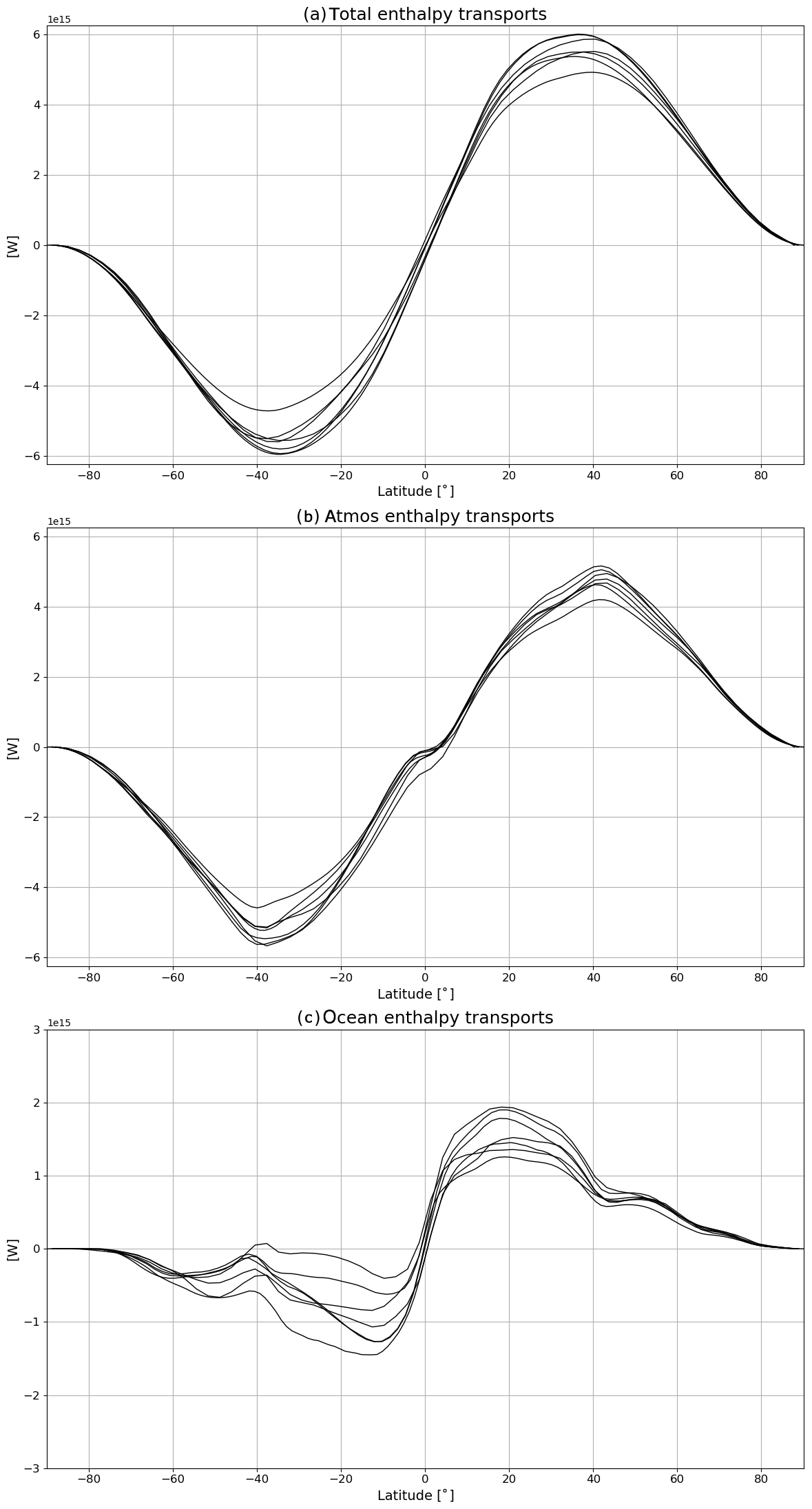
Figure 12Annual mean meridional sections of zonal mean meridional total (a), atmospheric (b), and oceanic (c) heat transports for 12 CMIP5 models control runs. Transports are implied from meridionally integrating top-of-the-atmosphere (TOA), atmospheric, and surface energy budgets (Trenberth et al., 2001) and then applying the usual correction accounting for energy imbalances, as in Carissimo et al. (1985). Values are in watts. Similar to Fig. 8 of Lembo et al. (2019) and produced with recipe_thermodyn_diagtool.yml; see details in Sect. 3.2.4.
3.2.5 Natural modes of climate variability and weather regimes
NCAR Climate Variability Diagnostic Package
Natural modes of climate variability co-exist with externally forced climate change and have large impacts on climate, especially at regional and decadal scales. These modes of variability are due to processes intrinsic to the coupled climate system and exhibit limited predictability. As such, they complicate model evaluation as the observational record is often not long enough to reliably assess the variability and confound assessments of anthropogenic influences on climate (Bengtsson and Hodges, 2019; Deser et al., 2012, 2014, 2017; Kay et al., 2015; Suárez-Gutiérrez et al., 2017). Despite their importance, systematic evaluation of these modes in Earth system models remains a challenge due to the wide range of phenomena to consider, the length of record needed to adequately characterize them, and uncertainties in the short observational datasets (Deser et al., 2010; Frankignoul et al., 2017; Simpson et al., 2018). While the temporal sequences of internal variability in models do not necessarily need to match those in the single realization of nature, their statistical properties (e.g. timescale, autocorrelation, spectral characteristics, and spatial patterns) need to be realistically simulated for credible climate projections.
In order to assess natural modes of climate variability in models, the NCAR Climate Variability Diagnostics Package (CVDP; Phillips et al., 2014) has been implemented into ESMValTool. The CVDP has been developed as a standalone tool. To allow for easy updating of the CVDP once a new version is released, the structure of the CVDP is kept in its original form and a single recipe recipe_CVDP.yml has been written to enable the CVDP to be run directly within ESMValTool. The CVDP facilitates evaluation of the major modes of climate variability, including ENSO (Deser et al., 2010), the Pacific Decadal Oscillation (PDO; Deser et al., 2010; Mantua et al., 1997), the Atlantic Multi-decadal Oscillation (AMO; Trenberth and Shea, 2006), the Atlantic Meridional Overturning Circulation (AMOC; Danabasoglu et al., 2012), and atmospheric teleconnection patterns such as the Northern and Southern Annular Modes (NAM and SAM; Hurrell and Deser, 2009; Thompson and Wallace, 2000), North Atlantic Oscillation (NAO; Hurrell and Deser, 2009), and Pacific North and South American (PNA and PSA; Thompson and Wallace, 2000) patterns. For details on the actual calculation of these modes in CVDP we refer to the original CVDP package and explanations available at http://www.cesm.ucar.edu/working_groups/CVC/cvdp/ (last access: 13 July 2020).
Depending on the climate mode analysed, the CVDP package uses the following variables: precipitation (pr), sea level pressure (psl), near-surface air temperature (tas), skin temperature (ts), snow depth (snd), sea ice concentration (siconc), and basin-average ocean meridional overturning mass stream function (msftmz). The models are evaluated against a wide range of observations and reanalysis data, for example, the Berkeley Earth System Temperature (BEST) for near-surface air temperature, the Extended Reconstructed Sea Surface Temperature v5 (ERSSTv5) for skin temperature, and ERA-20C extended with ERA-Interim for sea level pressure. Additional observations or reanalysis can be added by the user for these variables. The ESMValTool v2.0 recipe runs on all CMIP5 models. As an example, Fig. 13 shows the representation of ENSO teleconnections during the peak phase (December–February). Models produce a wide range of ENSO amplitudes and teleconnections. Note that even when based on over 100 years of record, the ENSO composites are subject to uncertainty due to sampling variability (Deser et al., 2017). Figure 14 shows the representation of the AMO as simulated by 41 CMIP5 models and observations during the historical period. The pattern of SSTA* associated with the AMO is generally realistically simulated by models within the North Atlantic basin, although its amplitude varies. However, outside of the North Atlantic, the models show a wide range of spatial patterns and polarities of the AMO.
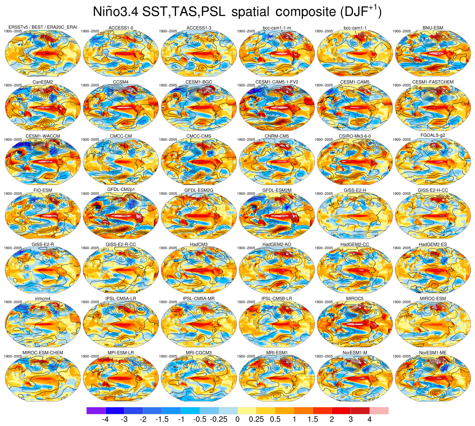
Figure 13Global ENSO teleconnections during the peak phase (December–February) as simulated by 41 CMIP5 models (individual panels labelled by model name) and observations (first row, upper left panel) for the historical period (1900–2005 for models and 1920–2017 for observations). These patterns are based on composite differences between all El Niño events and all La Niña events (using a ±1 standard deviation threshold of the Niño 3.4 SST Index) occurring in the period of record. Colour shading denotes SST and terrestrial TREFHT (surface air temperature at reference height) (∘C), and contours denote sea level pressure (psl); contour interval of 2 hPa, with negative values dashed). The period of record is given in the upper left of each panel. Observational composites use ERSSTv5 for SST, BEST for tas (near-surface air temperature), and ERA20C updated with ERA-I for psl. Figure produced with recipe_CVDP.yml.; see details in Sect. 3.2.5.
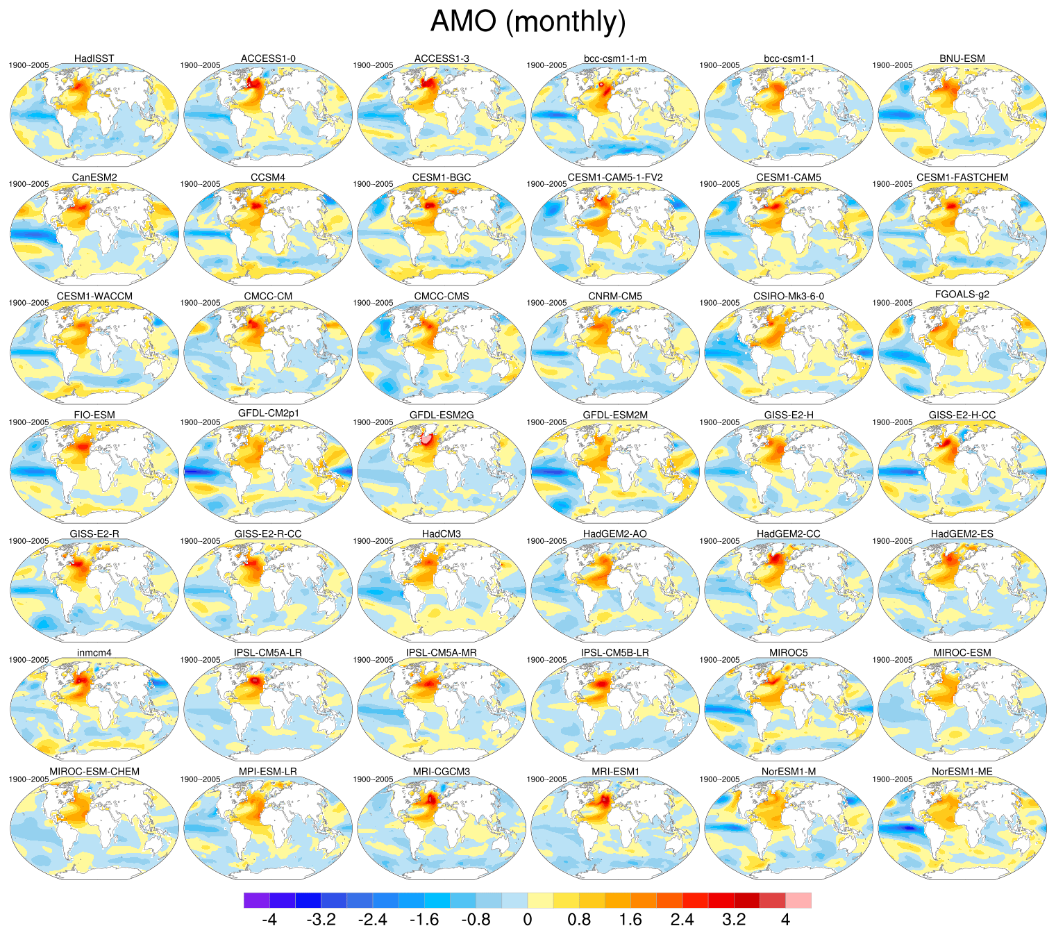
Figure 14Representation of the AMO in 41 CMIP5 models (individual panels labelled by model name) and observations (first row, upper left panel) for the historical period (1900–2005 for models and 1920–2017 for observations). These patterns are based regressing monthly SST anomalies (denoted SSTA*) at each grid box onto the time series of the AMO SSTA* Index (defined as SSTA* averaged over the North Atlantic 0–60∘ N, 80–0∘ W), where the asterisk denotes that the global (60∘ N–60∘ S) mean SSTA has been subtracted from SSTA at each grid box following Trenberth and Shea (2006). Figure produced with recipe_CVDP.yml; see details in Sect. 3.2.5.
Weather regimes
Weather regimes (WRs) refer to recurrent large-scale atmospheric circulation structures that allow the characterization of complex atmospheric dynamics in a particular region (Michelangeli et al., 1995; Vautard, 1990). The identification of WRs reduces the continuum of atmospheric circulation to a few recurrent and quasi-stationary (persistent) patterns. WRs have been extensively used to investigate atmospheric variability in the mid-latitudes, as they are associated with extreme weather events such as heat waves or droughts (Yiou et al., 2008). For example, there is a growing recognition of their significance especially over the Euro-Atlantic sector during the winter season, where four robust weather regimes have been identified – namely the NAO+, NAO−, Atlantic Ridge, and Scandinavian Blocking (Cassou et al., 2005). These WRs can also be used as a diagnostic to investigate the performance of state-of-the-art climate forecast systems: difficulties in reproducing the Atlantic Ridge and the Scandinavian Blocking have been often reported (Dawson et al., 2012; Ferranti et al., 2015). Forecast systems which are not able to reproduce the observed spatial patterns and frequency of occurrence of WRs may have difficulties in reproducing climate variability and its long-term changes (Hannachi et al., 2017). Hence, the assessment of WRs can help improve our understanding of predictability on intra-seasonal to interannual timescales. In addition, the use of WRs to evaluate the impact of the atmospheric circulation on essential climate variables and sectoral climatic indices is of great interest to the climate services communities (Grams et al., 2017). The diagnostic can be applied to model simulations under future scenarios as well. However, caution must be applied since large changes in the average climate, due to large radiative forcing, might affect the results and lead to somewhat misleading conclusions. In such cases further analysis will be needed to assess to what extent the response to climate change projects on the regimes patterns identified by the tool in the historical and future periods and to verify how future anomalies project onto the regime patterns identified in the historical period.
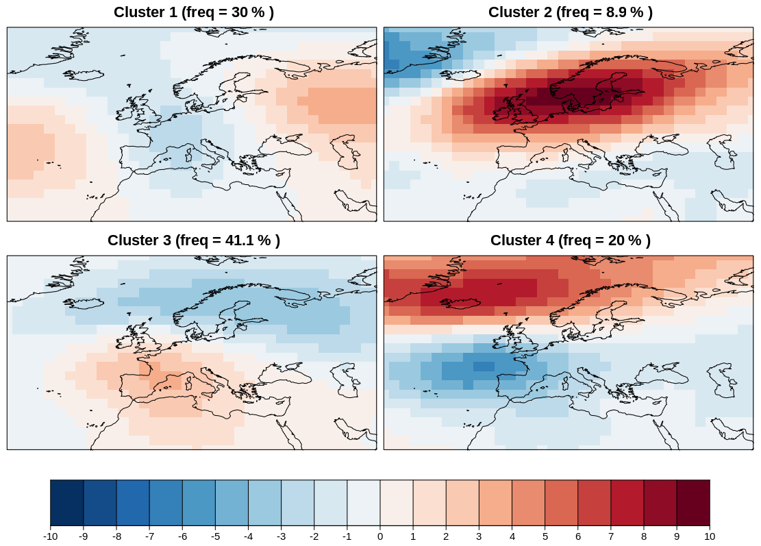
Figure 15Four modes of variability for autumn (September–October–November) in the North Atlantic European sector during the reference period 1971–2000 for the BCC-CSM1-1 historical simulations. The frequency of occurrence of each variability mode is indicated in the title of each map. The four clusters are reminiscent of the Atlantic Ridge, the Scandinavian Blocking, the NAO+, and the NAO− pattern. Result for recipe_modes_of_variability.yml; see details in Sect. 3.2.5.
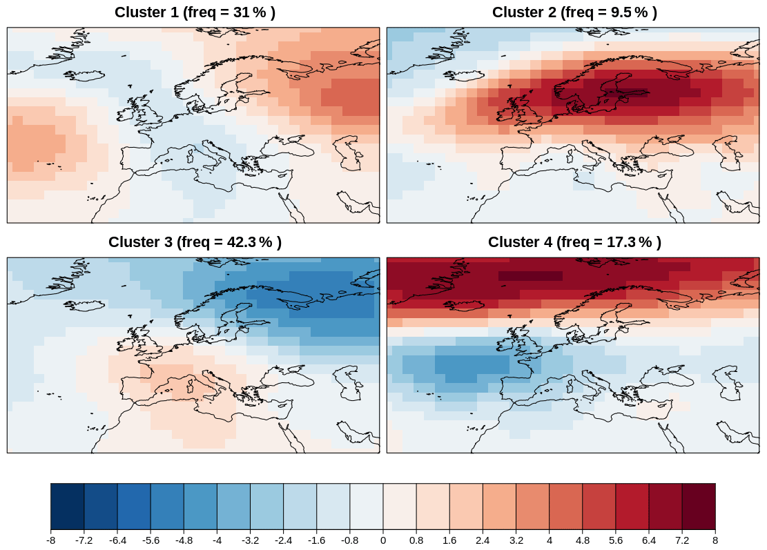
Figure 16Four modes of variability for autumn (September–October–November) in the North Atlantic European sector for the RCP 8.5 scenario using BCC-CSM1-1 future projection during the period 2020–2075. The frequency of occurrence of each variability mode is indicated in the title of each map. The four clusters are reminiscent of the Atlantic Ridge, the Scandinavian Blocking, the NAO+, and the NAO- pattern. Result for recipe_modes_of_variability.yml; see details in Sect. 3.2.5.
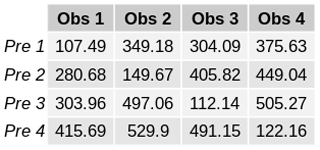
Figure 17RMSE between the spatial patterns obtained for the future “Pre” (2020–2075) and the reference “Obs” (1971–2000) modes of variability from the BCC-CSM1-1 simulations in autumn (September–October–November). Result for recipe_modes_of_variability.yml, see details in Sect. 3.2.5.
The recipe recipe_modes_of_variability.yml takes daily or monthly data from a particular region, season (or month), and period as input and then applies k mean clustering or hierarchical clustering either directly to the spatial data or after computing the EOFs. This recipe can be run for both a reference or observational dataset and climate projections simultaneously, and the root-mean-square error is then calculated between the mean anomalies obtained for the clusters from the reference and projection datasets. The user can specify the number of clusters to be computed. The recipe output consists of netCDF files of the time series of the cluster occurrences, the mean anomaly corresponding to each cluster at each location and the corresponding p value, for both the observed and projected WR and the RMSE between them. The recipe also creates three plots: the observed or reference modes of variability (Fig. 15), the reassigned modes of variability for the future projection (Fig. 16), and a table displaying the RMSE values between reference and projected modes of variability (Fig. 17). Low RMSE values along the diagonal show that the modes of variability simulated by the future projection (Fig. 16) match the reference modes of variability (Fig. 15). The recipe recipe_miles_regimes.yml integrates the diagnostics from the MiLES v0.51 tool (Davini, 2018) in order to calculate the four relevant North Atlantic weather regimes. This is done by analysing the 500 hPa geopotential height over the North Atlantic (30–87.5∘ N, 80∘ W–40∘ E). Once a 5 d smoothed daily seasonal cycle is removed, the EOFs which explain at least the 80 % of the variance are extracted in order to reduce the phase-space dimensions. A k mean clustering using Hartigan–Wong algorithm with k=4 is then applied providing the final weather regimes identification. The recipe compares multiple datasets against a reference one (default is ERA-Interim), producing multiple figures which show the pattern of each regime and its difference against the reference dataset. Weather regimes patterns and time series are provided in netCDF4 compressed zip format. Considering the limited physical significance of Euro-Atlantic weather regimes in other seasons, only winter is currently supported. An example output is shown in Fig. 18. The Atlantic Ridge regime, which is usually badly simulated by climate models, is reproduced with the right frequency of occupancy and pattern in MPI-ESM-MR when compared to ERA-Interim reanalysis.
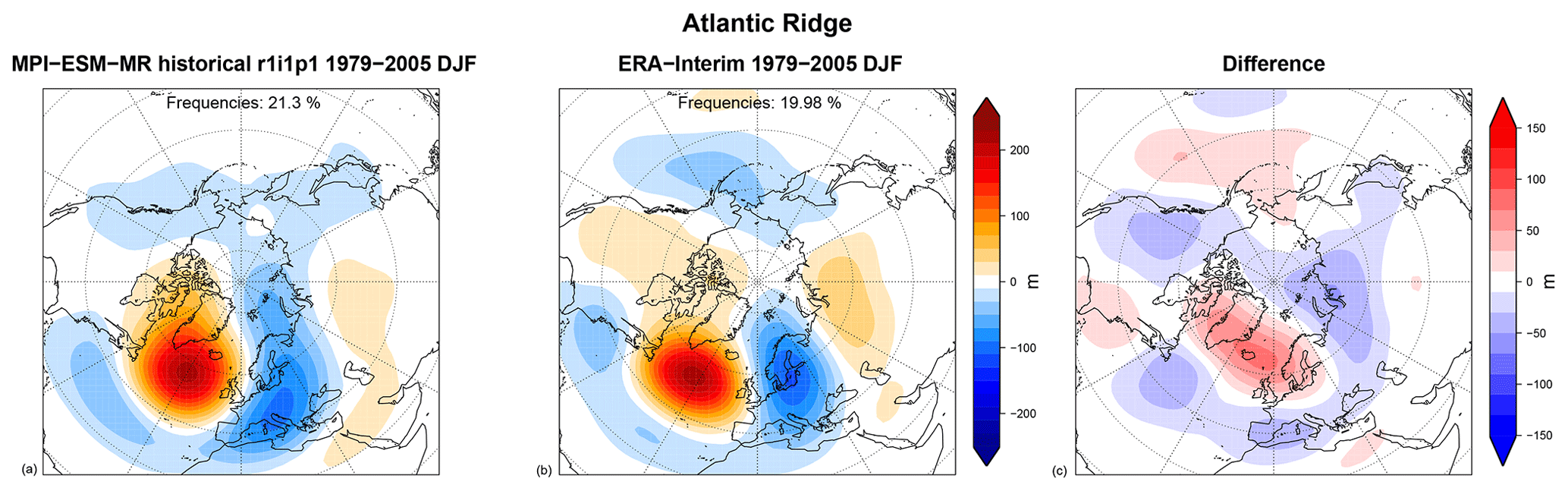
Figure 18500 hPa geopotential height anomalies (m) associated with the Atlantic Ridge weather regime over the 1979–2005 DJF period for (a) the CMIP5 MPI-ESM-MR historical r1i1p1 run, (b) the ERA-Interim reanalysis, and (c) their differences. The frequency of occupancy of each regime is reported at the top of each panel. Produced with recipe_miles_regimes.yml; see details in Sect. 3.2.5.
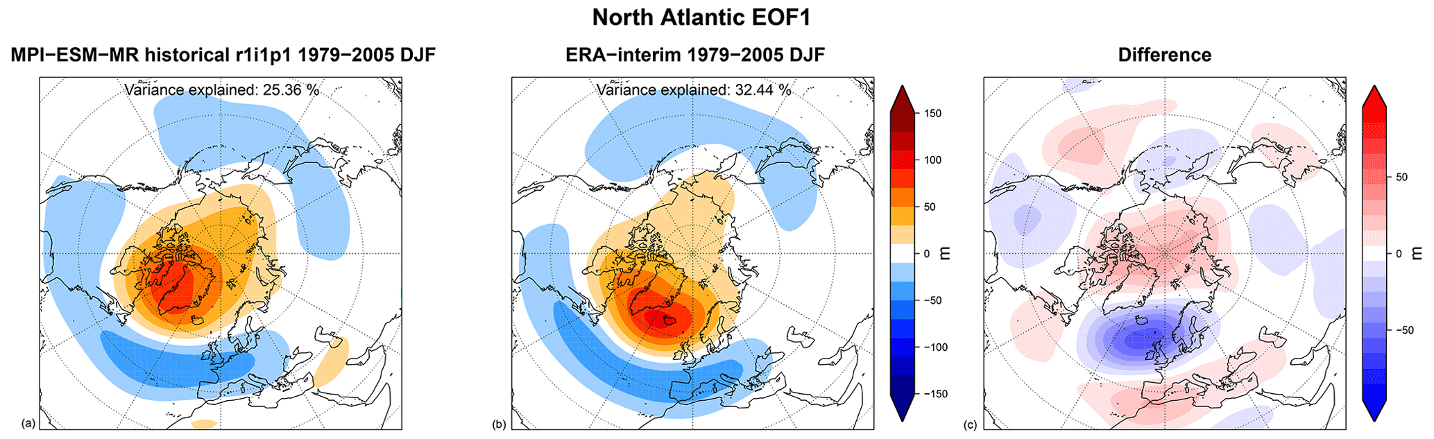
Figure 19Linear regression over the 500 hPa geopotential height (m) of the first North Atlantic EOF (i.e. the North Atlantic Oscillation, NAO) over the 1979–2005 DJF period for (a) the CMIP5 MPI-ESM-MR historical r1i1p1 run, (b) the ERA-Interim Reanalysis, and (c) their differences. The variance explained is reported at the top of each panel. Produced with recipe_miles_eof.yml; see details in Sect. 3.2.5.
Empirical orthogonal functions
EOF analysis is a powerful method to decompose spatiotemporal data using an orthogonal basis of spatial patterns. In weather sciences, EOFs have been extensively used to identify the most important modes of climate variability and their associated teleconnection patterns: for instance, the NAO (Ambaum, 2010; Wallace and Gutzler, 1981) and the Arctic Oscillation (AO; Thompson and Wallace, 2000) are usually defined with EOFs. Biases in the representation of the NAO or the AO have been found to be typical in many CMIP5 models (Davini and Cagnazzo, 2013).
The recipe recipe_miles_eof.yml integrates diagnostics from the MiLES v0.51 tool (Davini, 2018) in order to extract the first EOFs over a user-defined domain. Three default patterns are supported, namely the NAO (over the 20–85∘ N, 90∘ W–40∘ E box), the PNA (over the 20–85∘ N, 140∘ W–80∘ E box) and the AO (over the 20–85∘ N box). The computation is based on singular-value decomposition (SVD) applied to the anomalies of the monthly 500 hPa geopotential height. The recipe compares multiple datasets against a reference one (default is ERA-Interim), producing multiple figures which show the linear regressions of the principal component (PC) of each EOF on the monthly 500 hPa geopotential and its differences against the reference dataset. By default the first four EOFs are stored and plotted. As an example, Fig. 19 shows that the NAO is well represented by the MPI-ESM-LR model (which is used here for illustration), although the variance explained is underestimated and the northern centre of action, which is found close to Iceland in reanalysis, is displaced westward over Greenland.
Indices from differences between area averages
In addition to indices and modes of variability obtained from EOF and clustering analyses, users may wish to compute their own indices based on area-weighted averages or difference in area-weighted averages. For example, the Niño 3.4 index is defined as the sea surface temperature (SST) anomalies averaged over 5∘ N–5∘ S, 170–120∘ W. Similarly, the NAO index can be defined as the standardized difference between the weighted area-average mean sea level pressure of the domain bounded by 30–50∘ N, 0–80∘ W and 60–80∘ N, 0–80∘ W.
The functions for computing indices based on area averages in recipe_combined_indices.yml have been adapted to allow users to compute indices for the Niño 3, Niño 3.4, Niño 4, NAO, and the Southern Oscillation Index (SOI) defined region(s), with the option of selecting different variables (e.g. temperature of the ocean surface (tos, commonly named sea surface temperature) or pressure at sea level, psl, sea level pressure) with the option of computing standardized variables, applying running means and select different seasons by selecting the start and end months. The output of this recipe is a netCDF file containing a time series of the computed indices and a time series of the evolution of the index for individual models and the multi-model mean (see Fig. 20).
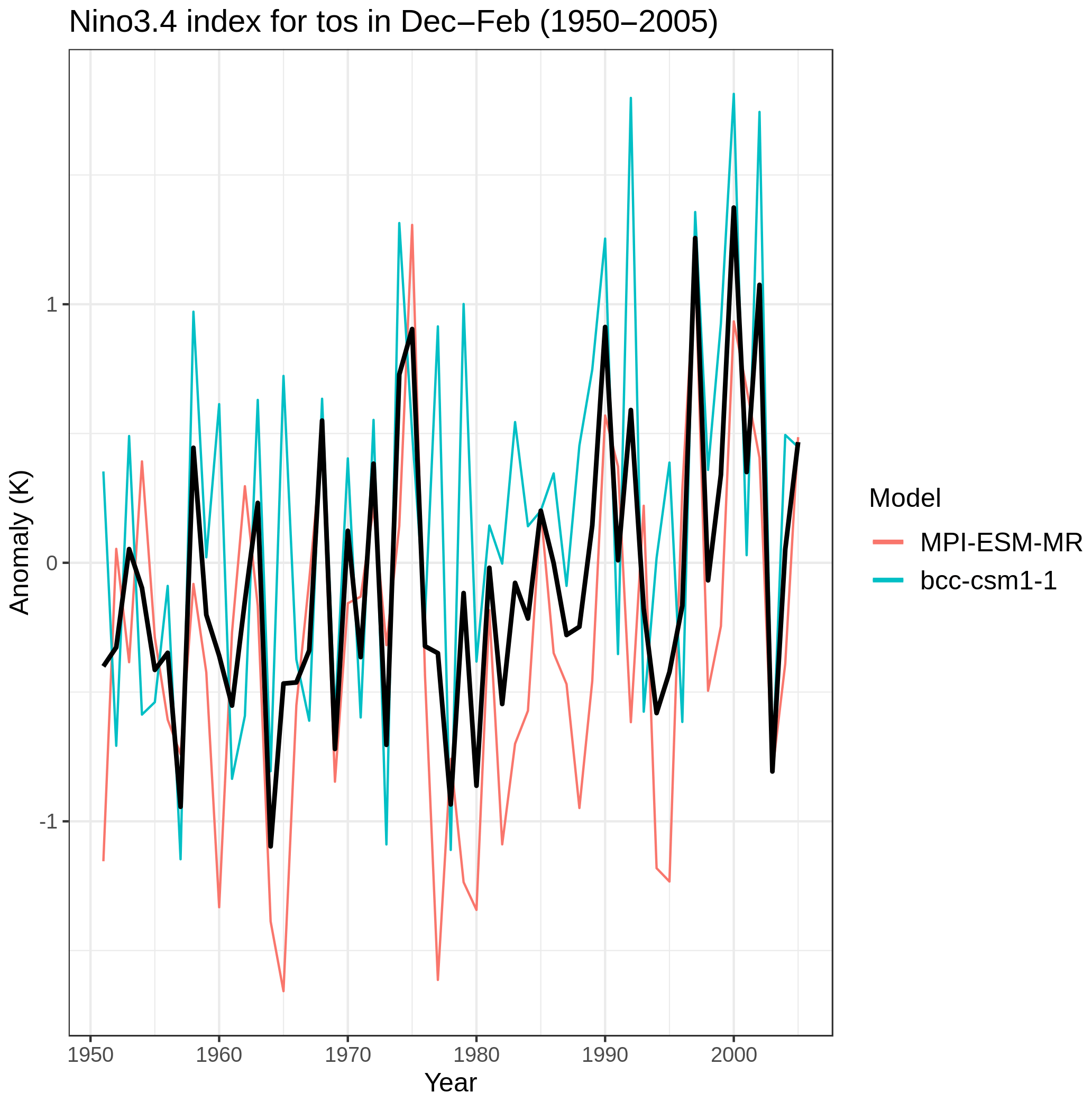
Figure 20Time series of the standardized sea surface temperature (tos) area averaged over the Niño 3.4 region during boreal winter (December–January–February). The time series correspond to the MPI-ESM-MR (red) and BCC-CSM1-1 (blue) models and their mean (black) during the period 1950–2005 for the ensemble r1i1p1 of the historical simulations. Produced with recipe_combined_indices.yml; see details in Sect. 3.2.5.
3.3 Diagnostics for the evaluation of processes in the ocean and cryosphere
3.3.1 Physical ocean
The global ocean is a core component of the Earth system. A significant bias in the physical ocean can impact the performance of the entire model. Several diagnostics exist in ESMValTool v2.0 to evaluate the broad behaviour of models of the global ocean. Figures 21–26 show several diagnostics of the ability of the CMIP5 models to simulate the global ocean. All available CF-compliant CMIP5 models are compared; however, each figure shown in this section may include a different set of models, as not all CMIP5 models produced all the required datasets in a CF-compliant format. To minimize noise, these figures are shown with a 6-year moving window average.
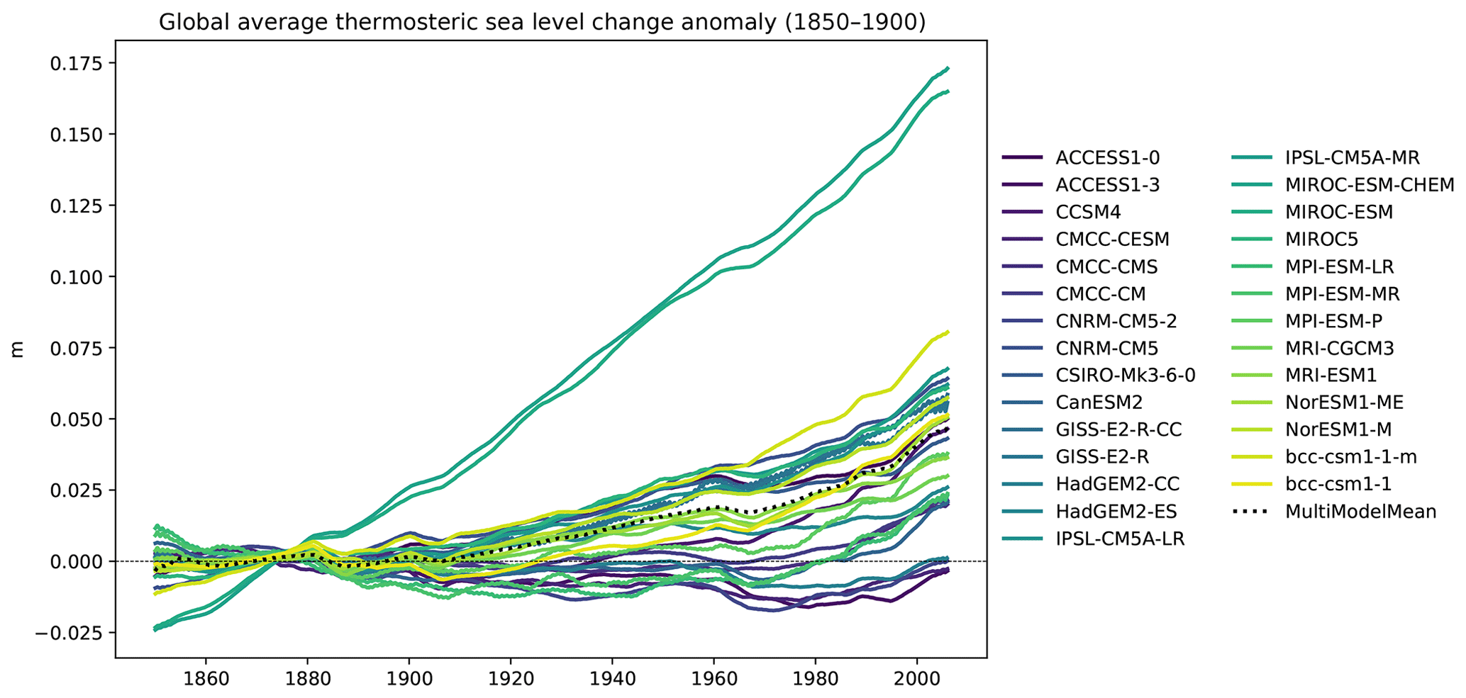
Figure 21The volume-weighted thermosteric sea level change anomaly in several CMIP5 models, in the historical experiment, and in the r1i1p1 ensemble member, with a 6-year moving average smoothing function. The anomaly is calculated against the mean of all years in the historical experiment before 1900. The multi-model mean is shown as a dashed line. Produced with recipe_ocean_scalar_fields.yml described in Sect. 3.3.1.
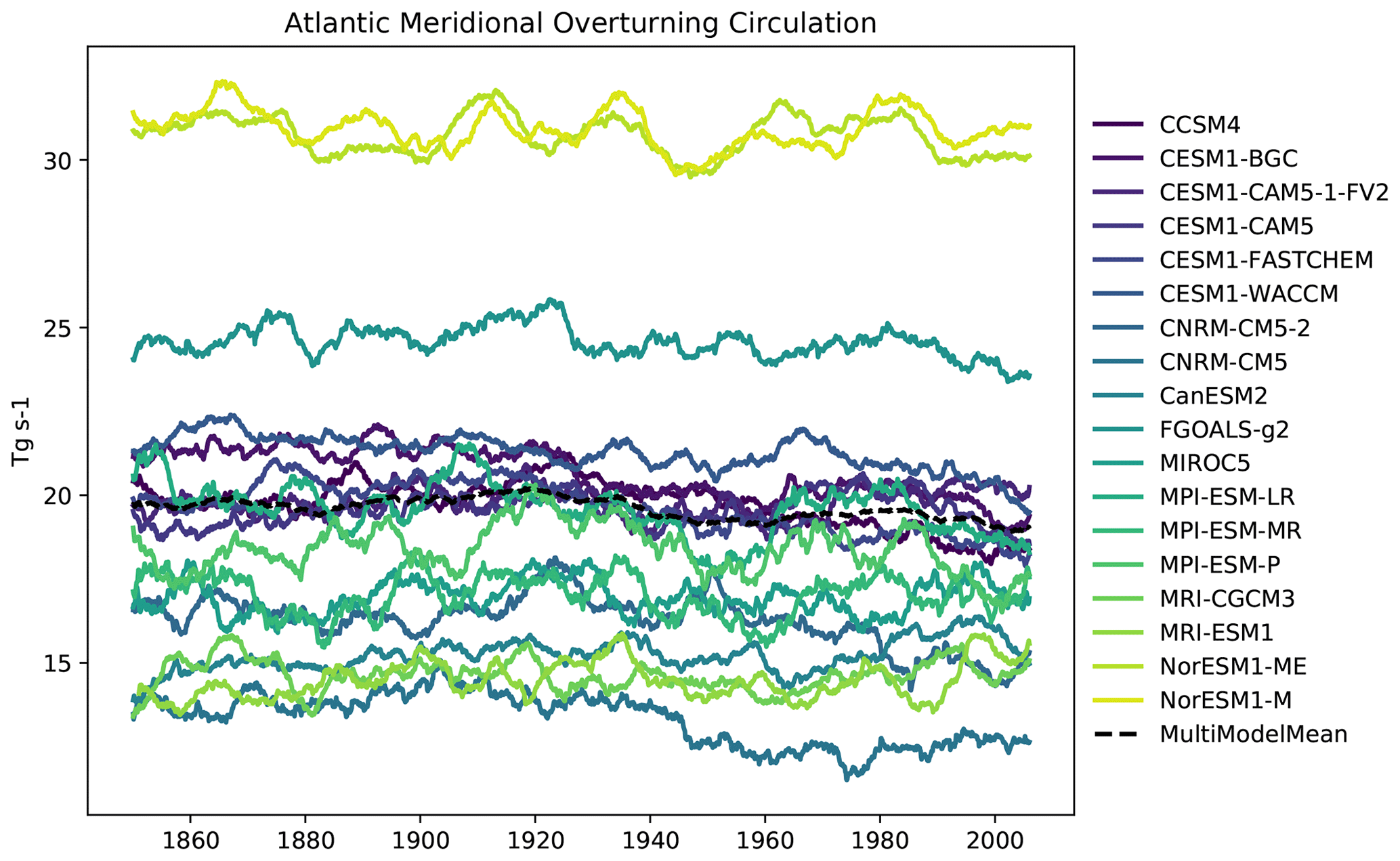
Figure 22The Atlantic Meridional Overturn Circulation (AMOC) in several CMIP5 models, in the historical experiment, and in the r1i1p1 ensemble member, with a 6-year moving average smoothing function. The multi-model mean is shown as a dashed line. The AMOC indicates the strength of the northbound current and this current transfers heat from tropical water to the North Atlantic. Produced with recipe_ocean_amoc.yml described in Sect. 3.3.1.
The volume-weighted global average temperature anomaly of the ocean is shown in Fig. 21 and displays the change in the mean temperature of the ocean relative to the start of the historical simulation. The temperature anomaly is calculated against the years 1850–1900. Nearly all CMIP5 models show an increase in the mean temperature of the ocean over the historical period. This figure was produced using the recipe recipe_ocean_scalar_fields.yml. The AMOC is an indication of the strength of the overturning circulation in the Atlantic Ocean and is shown in Fig. 22. It transfers heat from tropical waters to the northern Atlantic Ocean. The AMOC has an observed strength of 17.2 Sv (McCarthy et al., 2015). In the example shown in Fig. 22, all CMIP5 models show some interannual variability in the AMOC behaviour, but the decline in the multi-model mean over the historical period is not statistically significant. Previous modelling studies (Cheng et al., 2013; Gregory et al., 2005) have predicted a decline in the strength of the AMOC over the 20th century. The Drake Passage Current is a measure of the strength of the Antarctic Circumpolar Current (ACC). This is the strongest current in the global ocean and runs clockwise around Antarctica. The ACC was recently measured through the Drake Passage at 173.3±10.7 Sv (Donohue et al., 2016). Four of the CMIP5 models fall within this range (Fig. 23). Figures 22 and 23 were produced using the recipe recipe_ocean_amocs.yml. The global total flux of CO2 from the atmosphere into the ocean for several CMIP5 models is shown in Fig. 24. This figure shows the absorption of atmospheric carbon by the ocean. At the start of the historic period, most of the models shown here have been spun up, meaning that the air-to-sea flux of CO2 should be close to zero. As the CO2 concentration in the atmosphere increases over the course of the historical simulation, the flux of carbon from the air into the sea also increases.
Figure 23The Antarctic Circumpolar Current calculated through Drake Passage for a range of CMIP5 models in the historical experiment in the r1i1p1 ensemble member, with a 6-year moving average smoothing function. The multi-model mean is shown as a dashed line. Produced with recipe_ocean_amoc.yml described in Sect. 3.3.1.

Figure 24The global total air-to-sea flux of CO2 for a range of CMIP5 models in the historical experiment in the r1i1p1 ensemble member, with a 6-year moving average smoothing function. The multi-model mean is shown as a dashed line. Produced with recipe_ocean_scalar_fields.yml described in Sect. 3.3.1.
The CMIP5 models shown in Fig. 24 agree very closely on the behaviour of the air-to-sea flux of CO2 over the historical period, with all models showing an increase from close to zero and rising up to approximately 2 Pg of carbon per year (C yr−1) by the start of the 21st century. The global total integrated primary production from phytoplankton is shown in Fig. 25. Marine phytoplankton is responsible for 56±7 Pg C yr−1 of primary production (Buitenhuis et al., 2013), which is of similar magnitude to that of land plants (Field et al., 1998). In all cases, we do not expect to observe a significant change in primary production over the course of the historical period. However, the differences in the magnitude of the total integrated primary production inform us about the level of activity of the marine ecosystem. All CMIP5 models in Fig. 25 show little interannual variability in the integrated marine primary production, and there is no clear trend in the multi-model mean. Figures 24 and 25 were both produced with the recipe recipe_ocean_scalar_fields.yml. The combination of these five key time series figures allows a coarse-scale evaluation of the ocean circulation and biogeochemistry. The global volume-weighted temperature shows the effect of a warming ocean, while the change in the Drake Passage and the AMOC shows significant global changes in circulation. The integrated primary production shows changes in marine productivity, and the air–sea flux of CO2 shows the absorption of anthropogenic atmospheric carbon by the ocean.
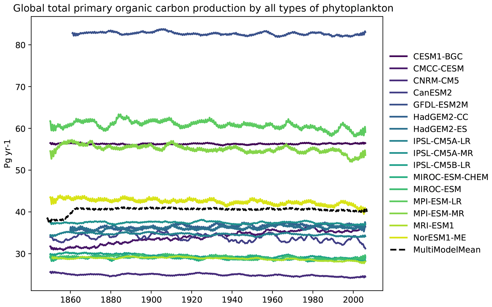
Figure 25The global total integrated primary production from phytoplankton for a range of CMIP5 models in the historical experiment in the r1i1p1 ensemble member, with a 6-year moving average smoothing function. The multi-model mean is shown as a dashed line. Produced with recipe_ocean_scalar_fields.yml described in Sect. 3.3.1.
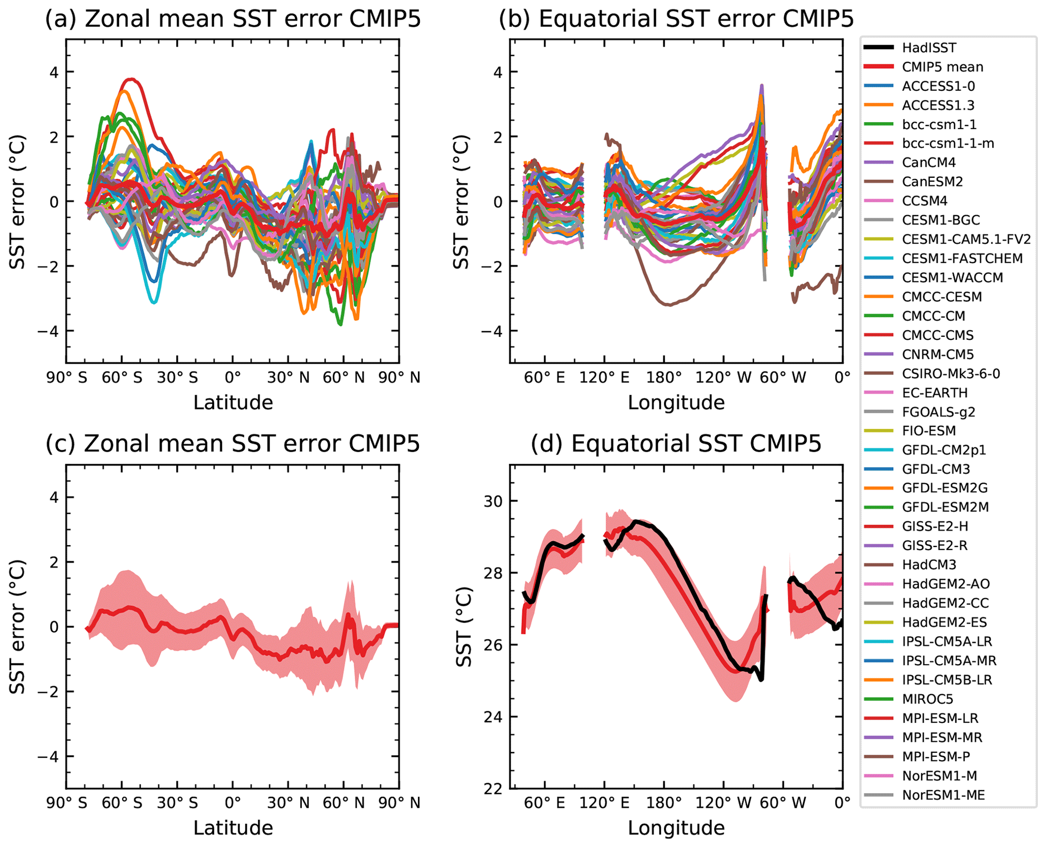
Figure 26(a) Zonally averaged sea surface temperature (SST) error in CMIP5 models. (b) Equatorial SST error in CMIP5 models. (c) Zonally averaged multi-model mean SST error for CMIP5 together with inter-model standard deviation (shading). (d) Equatorial multi-model mean SST in CMIP5 together with inter-model standard deviation (shading) and observations (black). Model climatologies are derived from the 1979–1999 mean of the historical simulations. The Hadley Centre Sea Ice and Sea Surface Temperature (HadISST; Rayner et al., 2003) observational climatology for 1979–1999 is used as a reference for the error calculation (a–c) and for observations in (d). Updated from Fig. 9.14 of IPCC WG I AR5 chap. 9 (Flato et al., 2013) and produced with recipe_flato13ipcc.yml; see details in Sect. 3.3.1.
In addition, a diagnostic from chap. 9 of IPCC AR5 for the ocean is added (Flato et al., 2013), which is included in recipe_flato13ipcc.yml. Figure 26 shows an analysis of the SST that documents the performance of models compared to one standard observational dataset, namely the SST part of the Hadley Centre Sea Ice and Sea Surface Temperature (HadISST) (Rayner et al., 2003) dataset. The SST plays an important role in climate simulations because it is the main oceanic driver of the atmosphere. As such, a good model performance for SST has long been a hallmark of accurate climate projections. In this figure we reproduce Fig. 9.14 of Flato et al. (2013). It shows both zonal mean and equatorial (averaged over 5∘ S to 5∘ N) SST. For the zonal mean it shows (a) the error compared to observations for the individual models and (c) the multi-model mean with the standard deviation. For the equatorial average it shows (b) the individual model errors and (d) the multi-model mean of the temperatures together with the observational dataset. In this way a good overview of both the error and the absolute temperatures can be provided for the individual model level. Figure 26 shows the overall good agreement of the CMIP5 models among themselves as well as compared to observations but also highlights the global areas with the largest uncertainty and biggest room for improvement. This is an important benchmark for the upcoming CMIP6 ensemble.
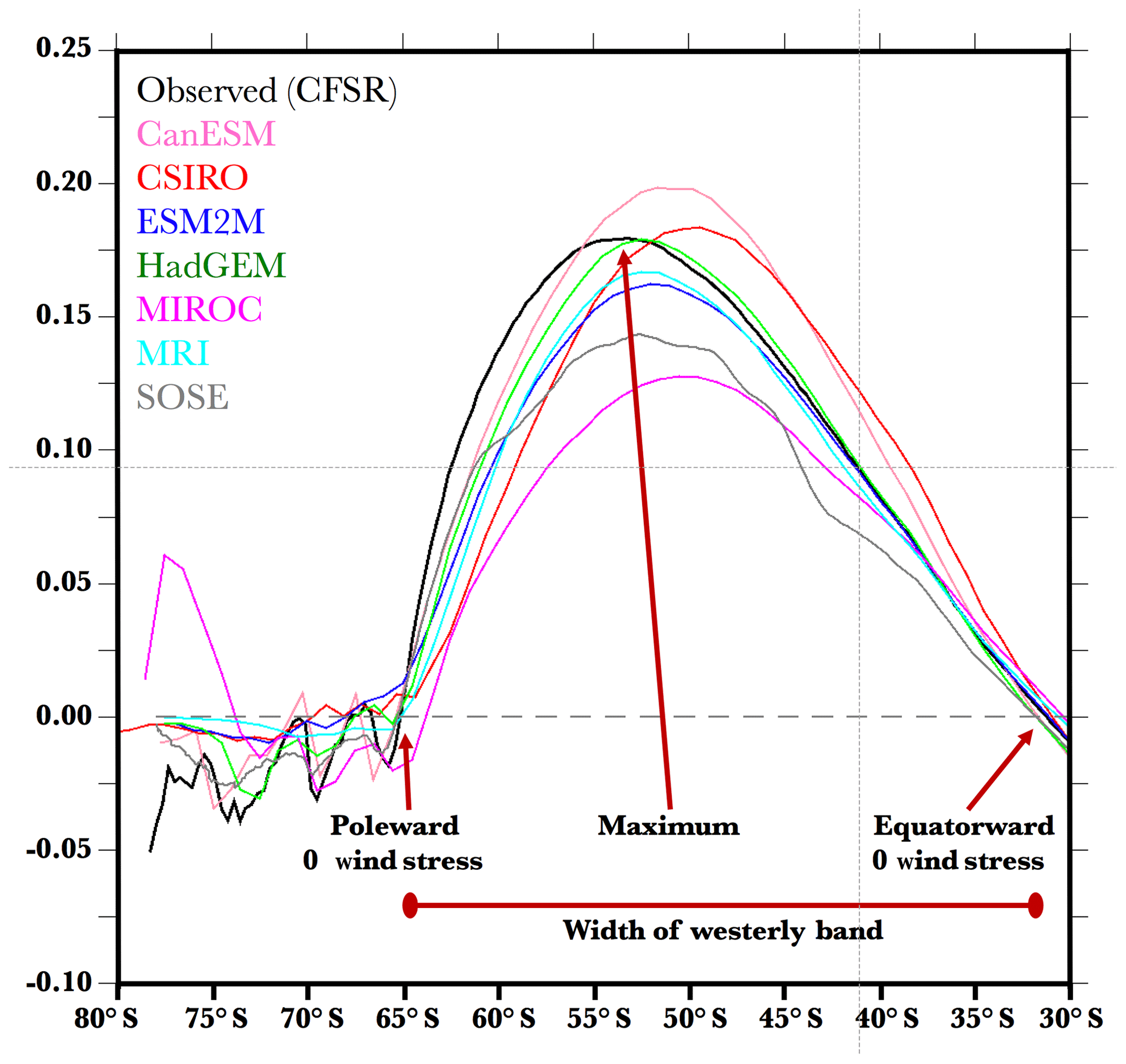
Figure 27The zonal and annual means of the zonal wind stress (N m−2) for the reanalysis, six of the CMIP5 simulations, and the B-SOSE (Biogeochemical - Southern Ocean State Estimate) – note that each of the model simulations (colours) and B-SOSE (grey) have the peak wind stress equatorward of the observations (black). Also shown are the latitudes of the observed “poleward zero wind stress” and the “equatorward zero wind stress” which delineate the “width of the westerly band” that is highly correlated with total heat uptake by the Southern Ocean. Enhanced from figure produced by recipe_russell18jgr.yml see Sect. 3.3.2. For further discussion of this figure; see the original in Russell et al. (2018).
3.3.2 Southern Ocean
The Southern Ocean is central to the global climate and the global carbon cycle and to the climate's response to increasing levels of atmospheric greenhouse gases, as it ventilates a large fraction of the global ocean volume. Roemmich et al. (2015) concluded that the Southern Ocean was responsible for 67 %–98 % of the total oceanic heat uptake; the oceanic increase in heat accounts for 93 % of the radiative imbalance at the top of the atmosphere. Global coupled climate models and Earth system models, however, vary widely in their simulations of the Southern Ocean and its role in and response to anthropogenic forcing. Due to the region's complex water mass structure and dynamics, Southern Ocean carbon and heat uptake depend on a combination of winds, eddies, mixing, buoyancy fluxes, and topography. Russell et al. (2018) laid out a series of diagnostic, observationally based metrics that highlight biases in critical components of the Southern Hemisphere climate system, especially those related to the uptake of heat and carbon by the ocean. These components include the surface fluxes (including wind and heat and carbon), the frontal structure, the circulation and transport within the ocean, the carbon system (in the ESMs), and the sea ice simulation. Each component is associated with one or more model diagnostics and with relevant observational datasets that can be used for the model evaluation. Russell et al. (2018) noted that biases in the strength and position of the surface westerlies over the Southern Ocean were indicative of biases in several other variables. The strength, extent, and latitudinal position of the Southern Hemisphere surface westerlies are crucial to the simulation of the circulation, vertical exchange and overturning, and heat and carbon fluxes over the Southern Ocean. The net transfer of wind energy to the ocean depends critically on the strength and latitudinal structure of the winds. Equatorward-shifted winds are less aligned with the latitudes of the Drake Passage and are situated over shallower isopycnal surfaces, making them less effective at both driving the ACC and bringing dense deep water up to the surface.
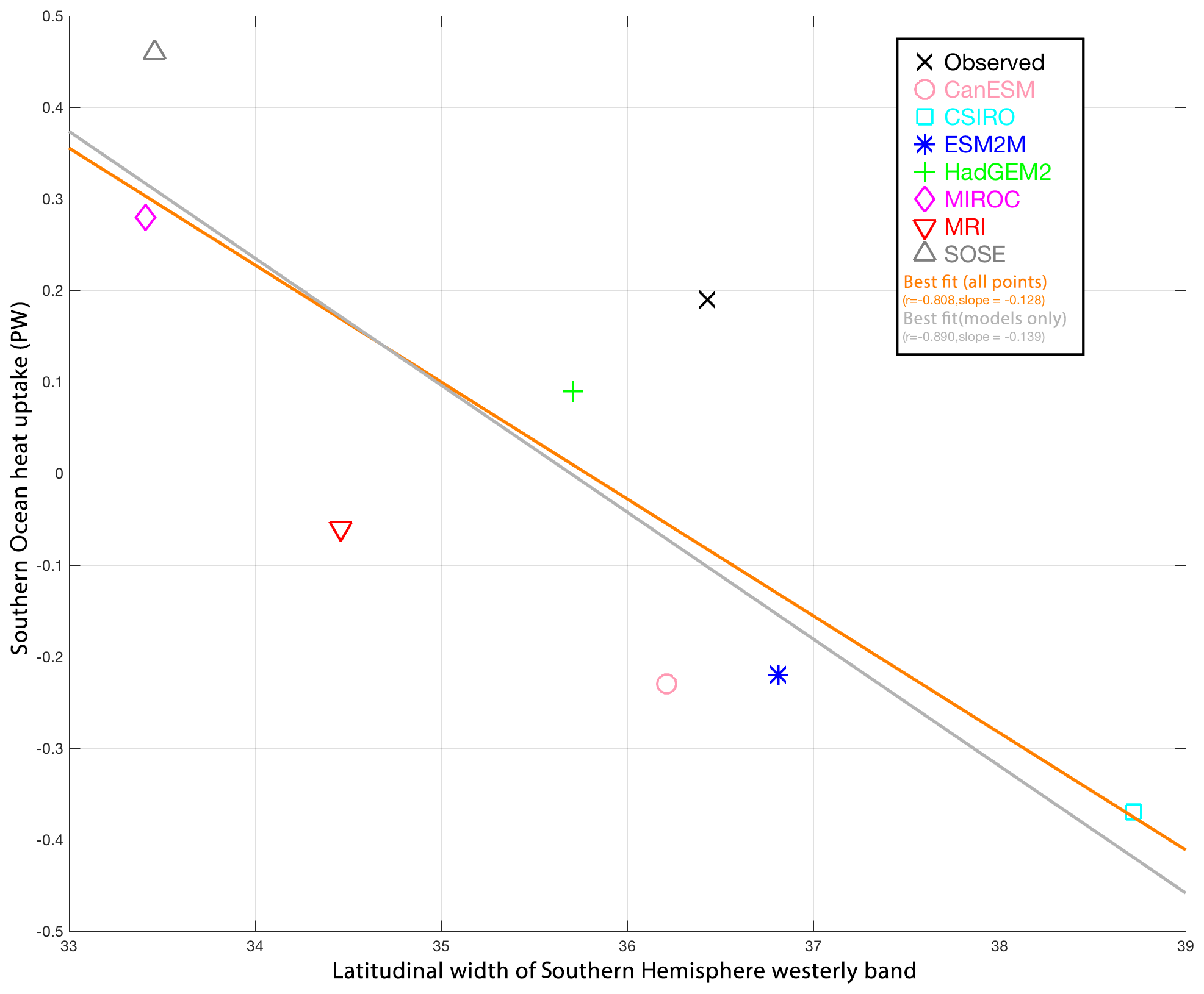
Figure 28Scatter plot of the width of the Southern Hemisphere westerly wind band (in degrees of latitude) against the annual-mean integrated heat uptake south of 30∘ S (in petawatts, PW – negative uptake is heat lost from the ocean), along with the “best fit” linear relationship for the models and observations shown. Enhanced from figure produced by recipe_russell18jgr.yml; see Sect. 3.3.2. For further discussion of this figure, see the original in Russell et al. (2018). The calculation of the “observed” heat flux into the Southern Ocean is described in the text. The correlation is significant above the 98 % level based on a simple t test.
Figure 27 shows the annually averaged, zonally averaged zonal wind stress over the Southern Ocean from a sample of the CMIP5 climate simulations and the equivalent quantity from the Climate Forecast System Reanalysis (Saha et al., 2013). While most model metrics indicate that simulations generally bracket the observed quantity, this metric indicates thatall of the models have an equatorward bias relative to the observations, an indication of a deeper modelling issue. Although Russell et al. (2018) only included six of the simulations submitted as part of CMIP5, the recipe recipe_russell18jgr.yml will recreate all of the metrics of this study for all CMIP5 simulations. Each metric assesses a simulated variable or a climatically relevant quantity calculated from one or more simulated variables (e.g. heat content is calculated from the simulated ocean temperature, thetao, while the meridional heat transport depends on both the temperature, thetao, and the meridional velocity, vo) relative to the observations. The recipe focuses on factors affecting the simulated heat and carbon uptake by the Southern Ocean. Figure 28 shows the relationship between the latitudinal width of the surface westerly winds over the Southern Ocean with the net heat uptake south of 30∘ S – the correlation (−0.8) is significant above the 98 % level.
3.3.3 Arctic Ocean
The Arctic Ocean is one of the areas of the Earth where the effects of climate change are especially visible today. The two most prominent processes are Arctic atmospheric temperature warming amplification (Serreze and Barry, 2011) and a decrease in the sea ice area and thickness (see Sect. 3.3.2). Both receive good coverage in the literature and are already well-studied. Much less attention is paid to the interior of the Arctic Ocean itself. In order to increase our confidence in projections of the Arctic climate future, proper representation of the Arctic Ocean hydrography is necessary.

Figure 29Mean (1970–2005) vertical potential temperature distribution in the Eurasian Basin for CMIP5 coupled ocean models, PHC3 climatology (dotted red line), and multi-model mean (dotted black line). Similar to Fig. 7 of Ilıcak et al. (2016) and produced with recipe_arctic_ocean.yml; see details in Sect. 3.3.3.
The vertical structure of temperature and salinity (T and S) in the ocean model is a key diagnostic that is used for ocean model evaluation. Realistic temperature and salinity distributions mean that the models properly represent dynamic and thermodynamic processes in the ocean. Different ocean basins have different hydrological regimes, so it is important to perform analysis of vertical T–S distribution for different basins separately. The basic diagnostics in this sense are the mean vertical profiles of temperature and salinity over some basin averaged for a relatively long period of time. Figure 29 shows the mean (1970–2005) vertical ocean potential temperature distribution in the Eurasian Basin of the Arctic Ocean as produced with recipe_arctic_ocean.yml. It shows that CMIP5 models tend to overestimate temperature in the interior of the Arctic Ocean and have too deep Atlantic water depth. In addition to individual vertical profiles for every model, we also show the mean over all participating models and similar profiles from climatological data (PHC3; Steele et al, 2001). The characteristics of vertical T–S distribution can change with time, and consequently the vertical T–S distribution is an important indicator of the behaviour of the coupled ocean–sea-ice–atmosphere system in the North Atlantic and Arctic oceans. One way to evaluate these changes is by using Hovmöller diagrams. We have created Hovmöller diagrams for two main Arctic Ocean basins – the Eurasian and Amerasian ones (as defined in Holloway et al., 2007), with T and S spatially averaged on a monthly basis for every vertical level. This diagnostic allows the temporal evolution of vertical ocean potential temperature distribution to be assessed. The T–S diagrams allow the analysis of water masses and their potential for mixing. The lines of constant density for specific ranges of temperature and salinity are shown against the background of the T–S diagram. The dots on the diagram are individual grid points from a specified region at all model levels within user-specified depth range. The depths are colour coded. Examples of the mean (1970–2005) T–S diagram for the Eurasian Basin of the Arctic Ocean shown in Fig. 30 refer to recipe_arctic_ocean.yml. Most models cannot properly represent Arctic Ocean water masses and either have wrong values for temperature and salinity or miss specific water masses completely.
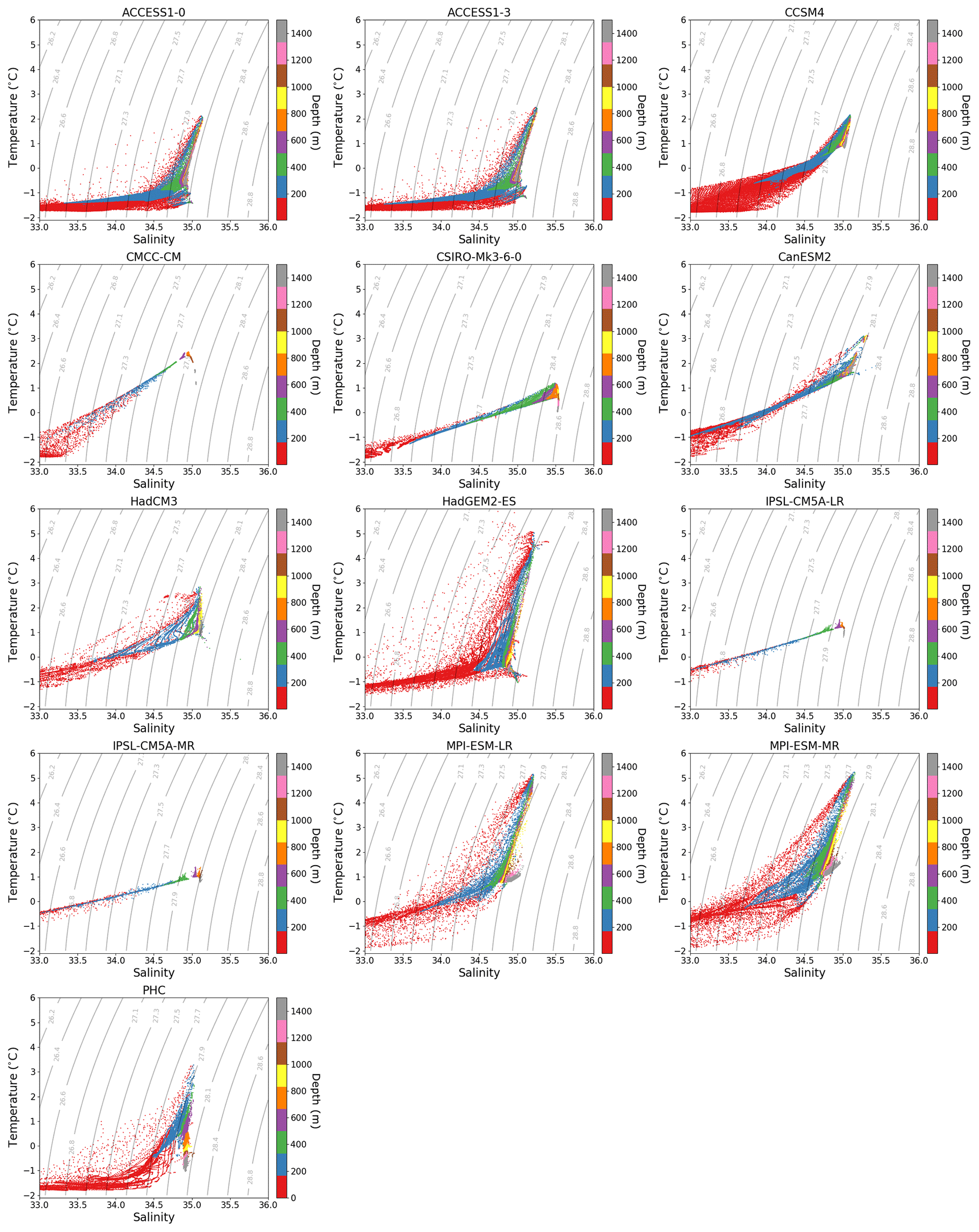
Figure 30Mean (1970–2005) T–S diagrams for Eurasian Basin of the Arctic Ocean. PHC3.0 shows climatological values for selected CMIP5 models and PHC3.0 observations. Produced with recipe_arctic_ocean.yml; see details in Sect. 3.3.3.
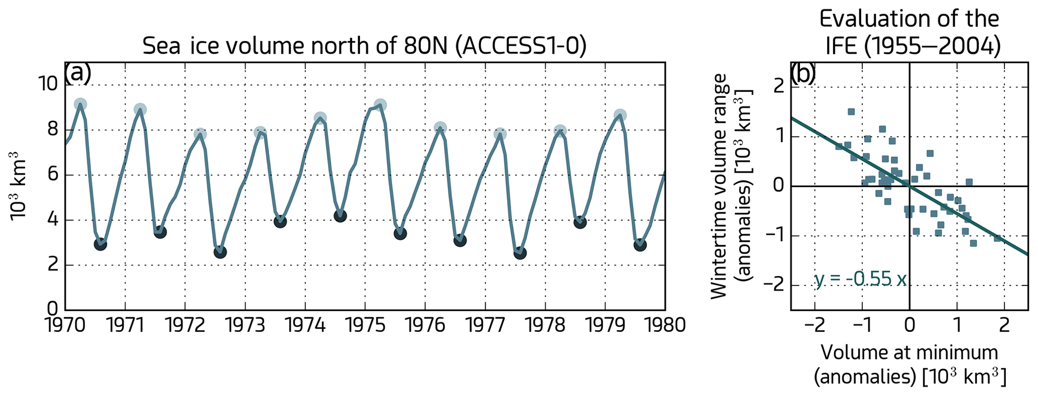
Figure 31Quantitative evaluation of the ice formation efficiency (IFE). (a) Example time series (1970–1979) of the monthly mean Arctic sea ice volume north of 80∘ N of one CMIP5 model (ACCESS1-0), with its annual minimum and maximum values marked with the dark and light dots, respectively. (b) Estimation of the IFE, defined as the regression between anomalies of sea ice volume produced during the growing season (difference between one annual maximum and the preceding minimum) and anomalies of the preceding minimum. A value of IFE = −1 means that the late-summer ice volume anomaly is fully recovered during the following winter (strong negative feedback damping all anomalies), while a value of IFE = 0 means that the wintertime volume production is essentially decoupled from the late-summer anomalies (inexistent feedback). Similar to extended data Fig. 7a–b of Massonnet et al. (2018a) and produced with recipe_seaice_feedback.yml; see details in Sect. 3.3.4.
The spatial distribution of basic oceanographic variables characterizes the properties and spreading of ocean water masses. For the coupled models, capturing the spatial distribution of oceanographic variables is especially important in order to correctly represent the ocean–ice–atmosphere interface. We have implemented plots with spatial maps of temperature, salinity, and current speeds at original model levels. For temperature and salinity, we have also implemented spatial maps of model biases from the observed climatology with respect to PHC3 climatology. For the model biases, values from the original model levels are linearly interpolated to the climatology (PHC3) levels and then spatially interpolated from the model grid to the regular PHC3 climatology grid. Resulting fields show model performance in simulating the spatial distribution of temperature and salinity. Vertical transects through arbitrary sections are important for an analysis of the vertical distribution of ocean water properties. Therefore, diagnostics that allow for the definition of an arbitrary ocean section by providing a set of points on the ocean surface are also implemented. For each point, a vertical profile of temperature or salinity on the original model levels is interpolated. All profiles are then connected to form a transect. The great-circle distance between the points is calculated and used as along-track distance. One of the main use cases for transects is to create vertical sections across ocean passages. Transects that follow the pathway of the Atlantic water according to Ilıcak et al. (2016) are also included. Atlantic water is a key water mass of the Arctic Ocean and its proper representation is one of the main challenges in Arctic Ocean modelling. A diagnostic that calculates the temperature of the Atlantic water core for every model as the maximum potential temperature between 200 and 1000 m depth in the Eurasian Basin is included. The depth of the Atlantic water core is calculated as the model level depth where the maximum temperature is found in Eurasian Basin (Atlantic water core temperature). In order to evaluate the spatial distribution of Atlantic water in different climate models, we also provide diagnostics with maps of the spatial distribution of water temperature at the depth of Atlantic water core in recipe_arctic_ocean.yml.
3.3.4 Sea ice
Sea ice is a critical component of the climate system, which considerably influences the ocean and atmosphere through different processes and feedbacks (Goosse et al., 2018). In the Arctic, sea ice has been dramatically retreating (Stroeve and Notz, 2018) and thinning (Kwok, 2018) in the past decades (Meredith et al., 2019). In the Antarctic, the sea ice cover has exhibited no significant change over the period of satellite observations, although this is the result of regional compensations and large interannual variability (Meredith et al., 2019). Climate models constitute a useful tool to make projections of the future changes in sea ice (Massonnet et al., 2012). However, the different climate models largely disagree on the magnitude of sea ice changes, even for the same forcing (Stroeve et al., 2012). One reason could be the different treatment of thermodynamic and dynamic processes and feedbacks related to sea ice.
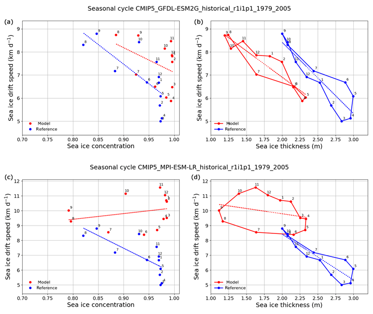
Figure 32Scatter plots of modelled (red) and observed (blue) monthly mean sea ice drift speed against sea ice concentration (a, c) and sea ice thickness (b, d) temporally averaged over the period 1979–2005 and spatially averaged over the SCICEX box. Panels (a, b) show results from the GDFL-ESM2G model and (c, d) show results from the MPI-ESM-LR model (CMIP5 historical runs). Observations/reanalysis are shown in all panels (IABP for drift speed, OSI-450 for concentration, and PIOMAS for thickness). Numbers denote months. Dotted lines show linear regressions. This figure was produced in a similar way to Fig. 4 of Docquier et al. (2017) with recipe_sea_ice_drift.yml; see details in Sect. 3.3.4.
In order to better understand and reduce model errors, two recipes related to sea ice have been implemented in ESMValTool v2.0. The first recipe, recipe_seaice_feedback.yml, is related to the negative sea ice growth–thickness feedback (Massonnet et al., 2018b). In this recipe, one process-based diagnostic named the ice formation efficiency (IFE) is computed based on monthly mean sea ice volume estimated north of 80∘ N. The diagnostic intends to evaluate the strength of the negative sea ice thickness–growth feedback, which causes late-summer negative anomalies in sea ice area and volume to be partially recovered during the next growing season (Notz and Bitz, 2017). To estimate the strength of that feedback, anomalies of the annual minimum of sea ice volume north of 80∘ N are first estimated. Then, the increase in sea ice volume until the next annual maximum is computed for each year. The IFE is defined as the regression of this ice volume production onto the baseline summer volume anomaly (Fig. 31). All CMIP5 models, without exception, simulate negative IFE over the historical period, implying that all these models display a basic mechanism of ice volume recovery when large negative anomalies occur in late summer. However, the strength of the IFE is simulated very differently by the models (Massonnet et al., 2018a). The IFE is closely associated with the annual mean sea ice volume north of 80∘ N. Also, the strength of the IFE is directly connected to the long-term variability, providing prospects for the application of emergent constraints. However, the shortness of observational records of sea ice thickness and their large uncertainty preclude rigorous applications of such constraints. The analyses nevertheless allow us (1) to pin down that the spread in CMIP5 sea ice volume projections is inherently linked to the way they represent the strength of sea ice feedbacks, and so their mean state, and (2) to provide guidance for the development of future observing systems in the Arctic, by stressing the need for more reliable estimates of sea ice thickness in the central Arctic basin (Ponsoni et al., 2019).
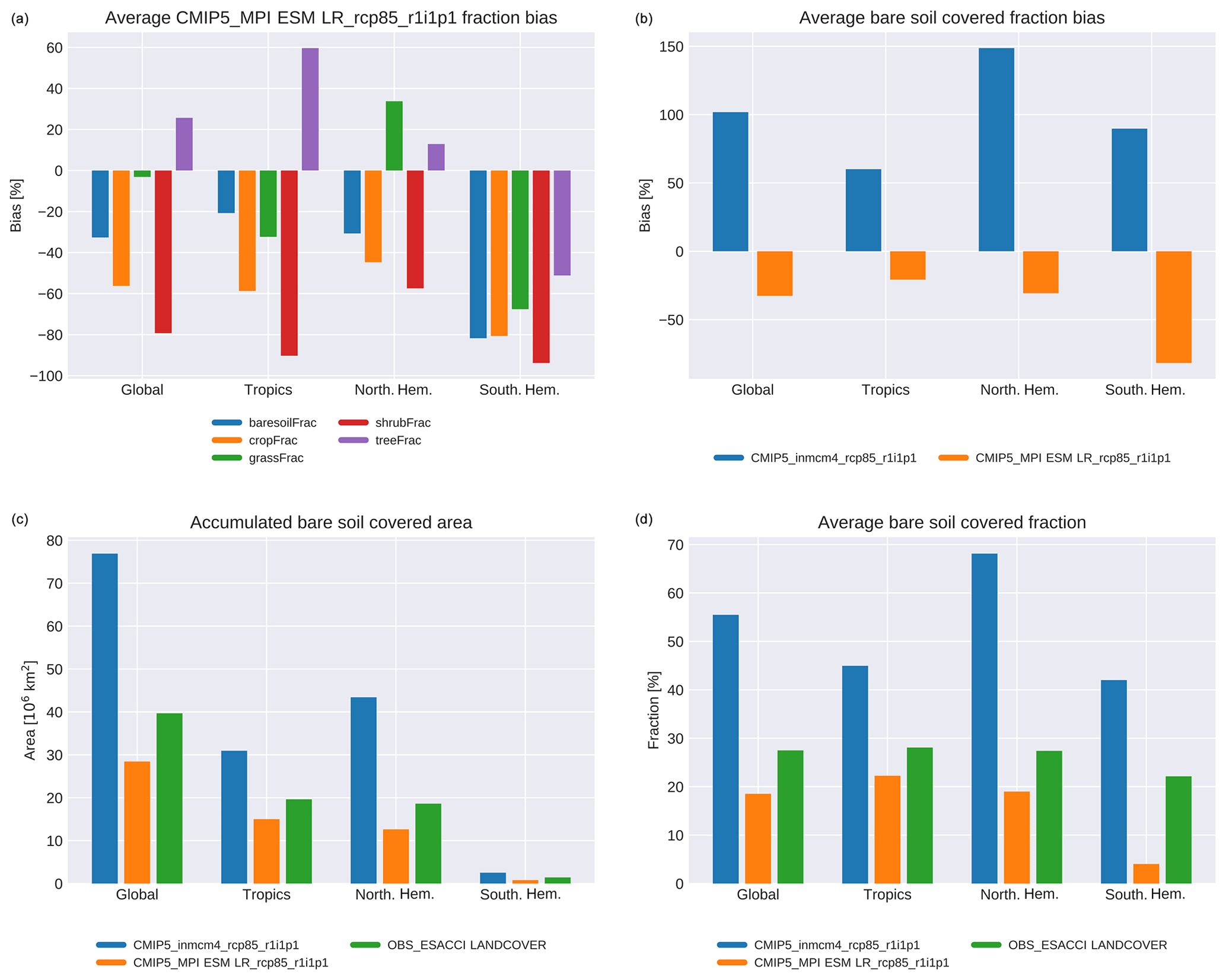
Figure 33The panels show plots produced by the metric recipe_landcover.yml using model output from historical CMIP5 simulations (period 2008–2012) of the ESMs MPI-ESM and INMCM4 compared to land cover observations provided by ESA CCI for different regions. Panels (a, b) display the relative bias (%) between the models M and the observation O computed as . This can be visualized either for one model (i.e. MPI-ESM) and several land cover types (a) or for one land cover type (i.e. bare soil fraction) and all selected models (b). Panels (c, d) display the area (106 km2) covered by a specific land cover type (i.e. bare soil fraction) for given regions (c), as well as the average cover fractions (%) (d) with respect to the total area of the regions. Thus, the land cover analysis provides a quick overview for major land cover types and the ability of different models to reproduce them. The metric is based on the analysis presented in Lauer et al. (2017) and Georgievski and Hagemann (2018) and discussed in Sect. 3.4.1.
The second recipe, recipe_sea_ice_drift.yml, allows us to quantify the relationships between Arctic sea ice drift speed, concentration, and thickness (Docquier et al., 2017). A decrease in concentration or thickness, as observed in recent decades in the Arctic Ocean (Kwok, 2018; Stroeve and Notz, 2018), leads to reduced sea ice strength and internal stress and thus larger sea ice drift speed (Rampal et al., 2011). Olason and Notz (2014) investigate the relationships between Arctic sea ice drift speed, concentration, and thickness using satellite and buoy observations. They show that both seasonal and recent long-term changes in sea ice drift are primarily correlated to changes in sea ice concentration and thickness. Our recipe allows quantifying these relationships in climate models. In this recipe, four process-based metrics are computed based on the multi-year monthly mean sea ice drift speed, concentration, and thickness, averaged over the central Arctic. The first metric is the ratio between the modelled drift-concentration slope and the observed drift-concentration slope. The second metric is similar to the first one, except that sea ice thickness is involved instead of sea ice concentration. The third metric is the normalized distance between the model and observations in the drift-concentration space. The fourth metric is similar to the third one, except that sea ice thickness is involved instead of sea ice concentration. Sea ice concentration from the European Organisation for the Exploitation of Meteorological Satellites Ocean and Sea Ice Satellite Application Facility (Lavergne et al., 2019), sea ice thickness from the Pan-Arctic Ice-Ocean Modeling and Assimilation System reanalysis (PIOMAS; Zhang and Rothrock, 2003), and sea ice drift from the International Arctic Buoy Programme (IABP; Tschudi et al., 2016) are used as reference products to compute these metrics (Fig. 32). Results in this example show that the GFDL-ESM2G model can reproduce the sea ice-drift speed–concentration–thickness relationships compared to observations, with higher drift speed with lower concentration or thickness, despite the ice which is too thin in the model, while the MPI-ESM-LR model cannot reproduce this result.
3.4 Diagnostics for the evaluation of land processes
3.4.1 Land cover
Land cover (LC) is either prescribed in the CMIP models or simulated using a dynamic global vegetation model (DGVM). Within the recent decade, numerous studies focused on the quantification of the impact of land cover change on climate (see Mahmood et al., 2014, and references therein for a comprehensive review). There is a growing body of evidence that vegetation, especially tree cover, significantly affects the terrestrial water cycle, energy balance (Alkama and Cescatti, 2016; Duveiller et al., 2018b), and carbon cycle (Achard et al., 2014). However, understanding the impact of LC change on climate remains controversial and is still work in progress (Bonan, 2008; Ellison et al., 2012; Mahmood et al., 2014; Sheil and Murdiyarso, 2009). In order to judge the LC-related ESM results, an independent assessment of the accuracy of the simulated spatial distributions of major land cover types is desirable to evaluate the DGVM accuracy for present climate conditions (Lauer et al., 2017).

Figure 34Potential albedo change due to a transition from land cover type “tree” to “crops and grasses” calculated through a multiple linear regression between the present-day land cover fractions (predictors) and albedo (predictands) within a moving window encompassing grid cells. Results are shown for (a) the MPI-ESM-LR model (2001–2005 July mean) and (b) the observational dataset from Duveiller et al. (2018a) (2008–2012 July mean). Produced with recipe_landcoveralbedo.yml; see details in Sect. 3.4.2 and in Lejeune et al. (2020).
Recently in the frame of the European Space Agency (ESA) Climate Change Initiative (CCI), a new global LC dataset has been published (Defourny et al., 2014, 2016) that can be used to evaluate or prescribe vegetation distributions for climate modelling. Effects of LC uncertainty in the ESA CCI LC dataset on land surface fluxes and climate are described by Hartley et al. (2017) and Georgievski and Hagemann (2018), respectively. Satellite-derived LC classes cannot directly be used for the evaluation of ESM vegetation due to the different concepts of vegetation representation in DGVMs, which are typically based on the concept of plant functional types (PFTs) that are supposed to represent groups of LC with similar functional behaviour. Thus, an important first step is to map the ESA CCI LC classes to PFTs as described by Poulter et al. (2015). As the PFTs in ESMs differ, the current LC diagnostic analyses only major LC types (bare soil, crops, grass, shrubs, trees), which is similar to the approach chosen by Brovkin et al. (2013) and Lauer et al. (2017). The corresponding evaluation metric was implemented into ESMValTool in recipe_landcover.yml. It evaluates areas, mean fractions, and biases compared to ESA CCI LC data over the land area of four major regions (global, tropics, northern and southern extratropics). Currently the evaluation uses ESA CCI LC data for the epoch 2008–2012 that have been generated with the ESA CCI LC user tool at 0.5∘ resolution. Consequently, model data are interpolated to the same resolution. For the calculation of mean fractions per major region, a land area of these regions needs to be specified and is currently taken from ESA CCI land cover. Example plots of accumulated area and biases in major LC types for different models are shown in Fig. 33.
3.4.2 Albedo changes associated with land cover transitions
Land cover changes (LCCs) can modify climate by altering land surface properties such as surface albedo, surface roughness, and evaporative fraction. In particular, historical deforestation since the pre-industrial era has led to an increase in surface albedo corresponding to a global radiative forcing of W m−2 (Myhre et al., 2013). There are however large uncertainties, even concerning the sign of the effect, regarding the impacts of LCC on near-surface temperature due to persistent model disagreement (Davin et al., 2020; de Noblet-Ducoudré et al., 2012; Lejeune et al., 2017; Pitman et al., 2009). These disagreements arise from uncertainties in (1) the interplay between radiative (albedo) and non-radiative processes (surface roughness and evaporative fraction), (2) the role of local versus large-scale processes and feedbacks (Winckler et al., 2017), and (3) the magnitude of change in given surface properties (e.g. albedo). Concerning the latter, Myhre et al. (2005) and Kvalevåg et al. (2010) suggest that the albedo change between natural vegetation and croplands is usually overestimated in climate simulations compared to satellite-derived observational evidence. In addition to this potential bias compared to observational data, there is a substantial spread in the model parameterizations for the albedo response to land cover perturbations. Boisier et al. (2012) identified that as being responsible for half of the dispersion in the albedo response to LCC since pre-industrial times among models participating in the LUCID project, whereas the remaining uncertainty was found to result from differences in the prescribed land cover. A more systematic evaluation of model performance in simulating LUC (land use change)-induced changes in albedo based on the latest available observations is therefore essential in order to reduce these uncertainties.
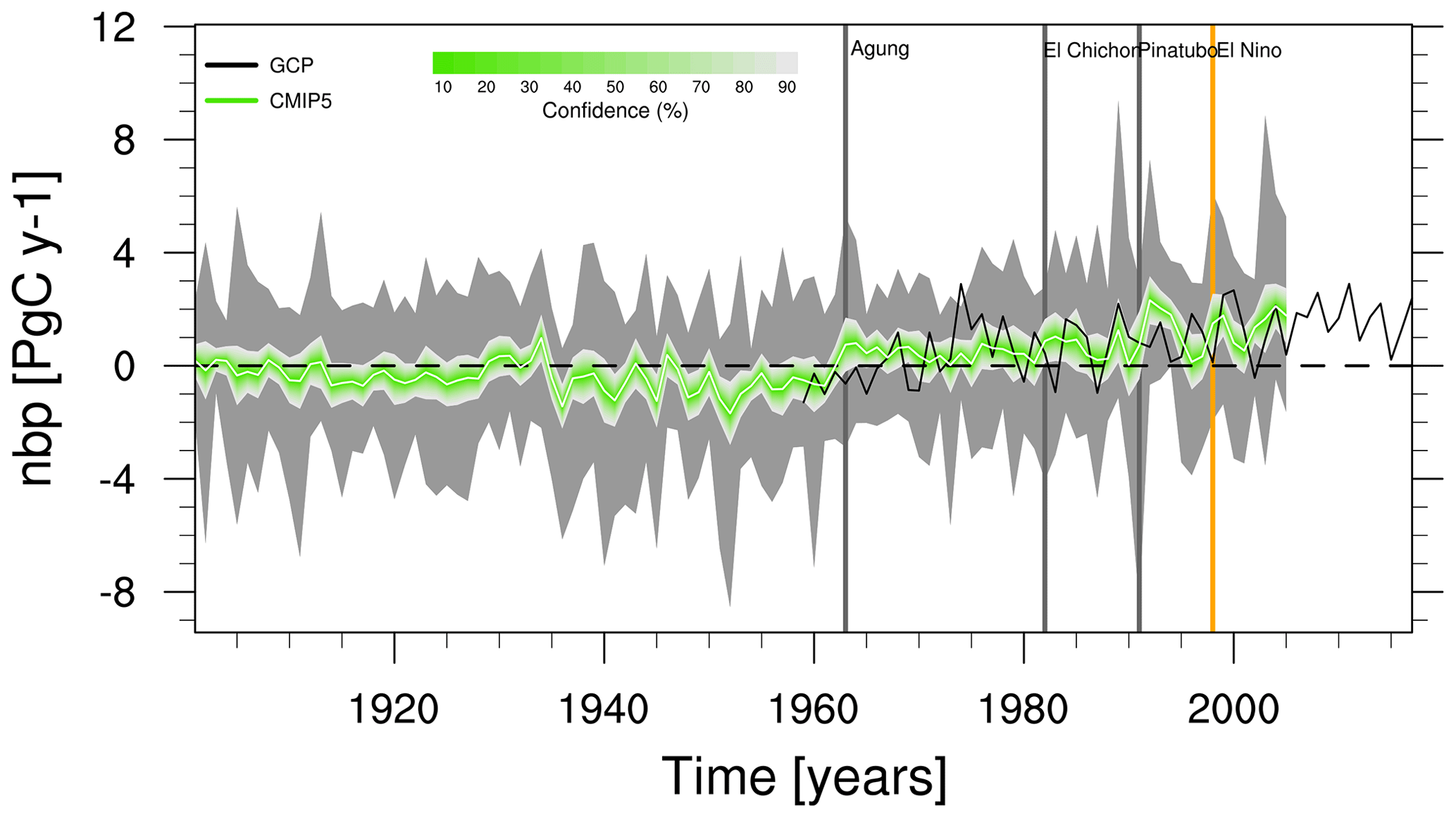
Figure 35Time series plot of the global land–atmosphere CO2 flux (nbp) for CMIP5 models compared to observational estimates from GCP (Le Quéré et al., 2018) (black line). Grey shading represents the range of the CMIP5 models; green shading shows the confidence interval evaluated from the CMIP5 ensemble standard deviation assuming a t distribution centred at the multi-model mean (white line). Vertical lines indicate volcanic eruptions (grey) and El Niño events (orange). Similar to Fig. 5 of Anav et al. (2013) and produced with recipe_anav13jclim.yml; see details in Sect. 3.5.1.
A satellite-based dataset providing a potential effect of a range of land cover transitions on the full surface energy balance (including albedo), at a global scale, 1∘ resolution, and monthly timescale is now available (Duveiller et al., 2018a). The potential albedo changes associated with vegetation transitions were extracted by a statistical treatment combining the ESA CCI LC data (see Sect. 3.4.1 for references) and the mean of the white-sky and black-sky albedo values of the NASA MCD43C3 albedo product for the 2008–2012 period (see Schaaf et al., 2002, for information on the retrieval algorithm). Because land-over-specific albedo values are not a standard output of climate models, in order to retrieve them a diagnostic was developed by Lejeune et al. (2020), which has been implemented into ESMValTool v2.0 in recipe_albedolandcover.yml. This approach determines the coefficients of multiple linear regressions between the albedo values and the tree, shrub, short vegetation (crops and grasses), and bare soil fractions of each grid cell within spatially moving windows encompassing model grid cells. These four LC classes correspond to the “IGBPgen” classification in Duveiller et al. (2018a). The recipe provides the option to run the algorithm on an interpolated grid or on the native model grid. The latter option was used in the example provided in Fig. 34. Solving these regressions provides the albedo values for trees, shrubs, and short vegetation (crops and grasses) from which the albedo changes associated with transitions between these three land cover types are derived. The diagnostic is applied to monthly data and, based on the value of the snow area fraction (snc), distinguishes between snow-free (snc < 0.1) and snow-covered (snc > 0.9) grid cells for each month. It can calculate albedo estimates for each of these two cases and each of the three land cover types, given that some criteria are fulfilled: the regressions are only conducted in the areas with a minimum number of 15 grid cells (either snow-free or snow-covered), taking into account only the grid cells where the sum of the area fractions occupied by the three considered land cover types exceeds 90 %. The algorithm eventually plots global maps of the albedo changes associated with the corresponding LC transitions for each model in their original resolution, next to the satellite-derived estimates from Duveiller et al. (2018a). The diagnostic shows data according to the IGBPgen classification, which entails only four LC classes that can be directly compared to model PFTs. An example plot is shown in Fig. 34 for the July albedo change associated with a transition from trees to short vegetation types (crops and grasses). Almost only snow-free areas are visible for this month, while grey areas indicate where the spatial co-existence of the two LC classes was not high enough for the regression technique to be performed, where the regression results did not pass the required quality checks, or where there were grid cells which could not be categorized either as snow-free or as snow-covered (Duveiller et al., 2018a). In the example shown here, the July albedo difference between trees and crops or grasses is about at least twice as high in the MPI-ESM-LR model as in the observations, strongly suggesting that the simulated summer albedo increase from historical land cover changes is overestimated in this model. The results reveal that the July albedo difference between trees and crops or grasses is about at least twice as high in the MPI-ESM-LR model as in the observations, strongly suggesting that the simulated summer albedo increase from historical LCC is overestimated in this model.
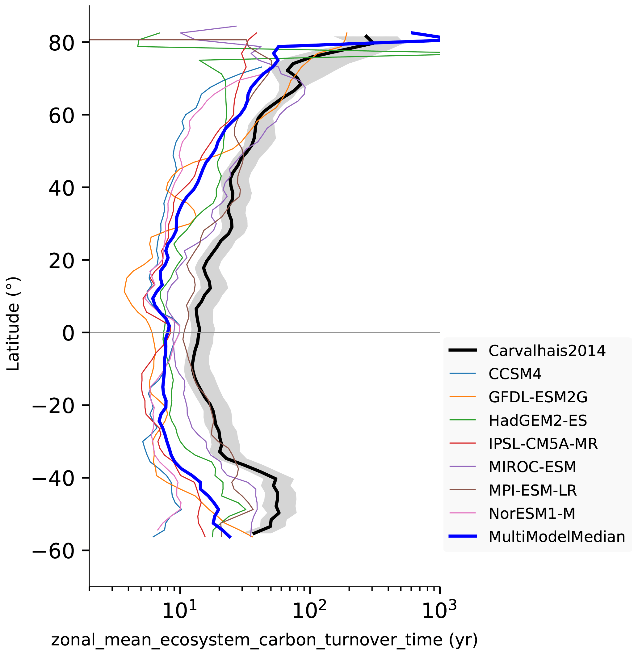
Figure 36Zonal distribution of ecosystem turnover time of carbon (in years). The zonal values are calculated as the ratio of total carbon stock and the gross primary productivity per latitude. The individual models are plotted as thin coloured lines, the multi-model ensemble as a thick blue line, and the observation-based estimate (Carvalhais et al., 2014) as a thick black line with shaded region showing the observational uncertainty. The median of all models is adopted as the multi-model ensemble. Note the logarithmic horizontal axis. Produced with recipe_carvalhais2014nat.yml; see details in Sect. 3.5.2.
3.5 Diagnostics for the evaluation of biogeochemical processes
3.5.1 Terrestrial biogeochemistry
With CO2 being the most important anthropogenic greenhouse gas, it is vital for ESMs to have a realistic representation of the carbon cycle. Atmospheric concentration of CO2 can be inferred from the difference between anthropogenic emissions and the land and ocean carbon sinks simulated by the models. These sinks are affected by atmospheric CO2 and climate change, thus introducing feedbacks between the climate system and the carbon cycle (Arora et al., 2013; Friedlingstein et al., 2006). The quantification of these feedbacks to estimate the evolution of these carbon sinks and thus the atmospheric CO2 concentration and the resulting climate change is paramount (Cox et al., 2013; Friedlingstein et al., 2014; Wenzel et al., 2014, 2016). The Anav et al. (2013) paper evaluated CMIP5 models in three different timescales: long-term trends, interannual variability, and seasonal cycles for the main climatic variables controlling both the spatial and temporal characteristics of the carbon cycle, i.e. surface land temperature (tas), precipitation over land (pr), sea surface temperature (tos), land–atmosphere (nbp) and ocean-atmosphere fluxes (fgco2), gross primary production (gpp), leaf area index (lai), and carbon content in soil and vegetation (cSoil, cVeg). Models are able to simulate key characteristics of the main climatic variables and their seasonal evolution, but deficiencies in the simulation of specific variables, especially in the land carbon cycle with a general overestimation of photosynthesis and leaf area index, as well as an underestimation of the primary production in the ocean exist.
The analysis from Anav et al. (2013) can be reproduced with recipe_anav13jclim.yml. In addition to the diagnostics already implemented in ESMValTool v1.0 and ported to v2.0, new diagnostics for the time series anomalies of tas, pr, and tos as well as time series for nbp and fgco2 have been added, reproducing Figs. 1, 2, 3, 5, and 13 of Anav et al. (2013), with the latter two also forming Fig. 26 of Flato et al. (2013). In ESMValTool v2.0, observational estimates of gpp are included from the latest data release of the FLUXCOM project (Jung et al., 2019), which integrates FLUXNET measurements, satellite remote sensing, and climate data with machine learning to provide improved global products of land–atmosphere fluxes for evaluation. The routines needed to make carbon and energy fluxes from the FLUXCOM project CMOR-compliant to facilitate process-based model evaluation is also made available as part of ESMValTool v2.0. As an example of the newly added plots, Fig. 35 shows the time series for the land–atmosphere carbon flux nbp, similar to Fig. 5 of Anav et al. (2013). Shading indicates the confidence interval of the CMIP5 ensemble standard deviation, derived from assuming a t distribution centred on the ensemble mean (inner curve), while the grey shading shows the overall range of variability of the models. As positive values correspond to a carbon uptake of the land, the plot shows a slight increase in the land carbon uptake over the whole period.
3.5.2 Ecosystem turnover times of carbon
The exchange of carbon between the land biosphere and atmosphere represents a key feedback mechanism that will determine the effect of global changes on the carbon cycle and vice versa (Heimann and Reichstein, 2008). Despite significant implications, the uncertainties in simulated land carbon stocks that integrate the land–atmosphere carbon exchange are large and, therefore, represent a major challenge for ESMs (Friedlingstein et al., 2014; Friend et al., 2014). One of the major factors leading to these uncertainties is the turnover time of carbon, the time period that a carbon atom on average spends in land ecosystems, from assimilation through photosynthesis to its release back into the atmosphere. This emergent ecosystem property, calculated, for example, as a ratio of long-term average total carbon stock to gross primary productivity, has been extensively used to evaluate ESM simulations (Carvalhais et al., 2014; Koven et al., 2015, 2017; Todd-Brown et al., 2013). Despite the large range of observational uncertainties and sources, ESM simulations consistently exhibit a robust correlation with the observation ensembles but with a substantial underestimation bias.
Carvalhais et al. (2014) evaluated the biases in ecosystem carbon turnover time in CMIP5 models and their associations with climate variables and then quantified multi-model biases and agreements. The recipe_carvalhais2014nat.yml reproduces the analysis of Carvalhais et al. (2014). It requires the simulations of total vegetation carbon content (cVeg), total soil carbon content (cSoil), gross primary productivity (gpp) as well as precipitation (pr), and near-surface air temperature (tas). As an example, an evaluation of the zonal means of turnover time in CMIP5 models is shown in Figure 36. The models follow the gradient of increasing turnover times of carbon from the tropics to higher latitudes, much related to temperature decreases, as observed in observations. However, for most of the latitudinal bands, with the exception of one model, most simulations reveal turnover times that are faster than the observations. Most CMIP5 models (and multi-model ensemble) have a much shorter turnover time than the observation-based estimate across the whole latitudinal range. Even though different estimates of observation-based carbon fluxes and stocks can vary significantly, a recent study by Fan et al. (2020), their Fig. 5a, shows that the zonal distributions of observation-based estimates of turnover time are robust against the differences in observations. The spread among the models is also large and can vary by 1 order of magnitude. This results not only in a large bias in turnover time but also a considerable disagreement among the models. In fact, the majority of CMIP5 models simulate a turnover time more than 4 times shorter than the observation-based estimate in most regions (Fig. 37). A generalized underestimation of turnover times of carbon is apparently dominant in water-limited regions. In most of these regions most models show estimates outside of the observational uncertainties (stippling). These results challenge the combined effects of water and temperature limitations on turnover times of carbon and suggest the need for an improvement on the description of the water cycle in terrestrial ecosystems. In arid and semi-arid regions model agreement is also low with 2 or fewer (out of 10) models within the observational uncertainty.
In addition, the recipe also produces the full factorial model–model–observation comparison matrix that can be used to evaluate individual models. It further provides a quantitative measure of turnover times across different biomes, as well as its relationship with precipitation and temperature.
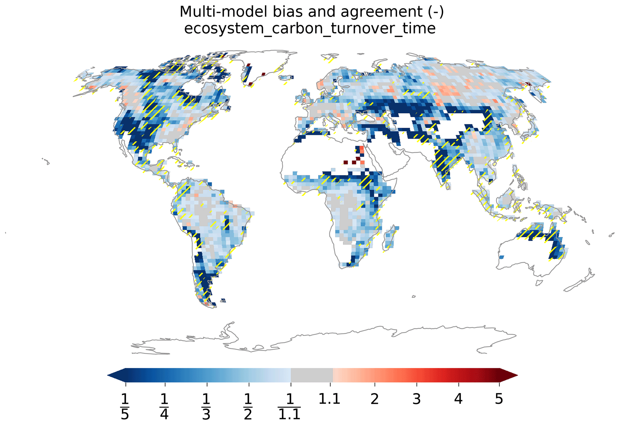
Figure 37Global distribution of the biases in the multi-model ensemble ecosystem turnover time of carbon (years) and the multi-model agreement in CMIP5 models. The bias is calculated as the ratio between multi-model ensemble and observation-based estimate (Carvalhais et al., 2014). The stippling indicates the regions where only two or fewer models (out of 10) are within the range of observational uncertainties (5th and 95th percentiles). Produced with recipe_carvalhais2014nat.yml; see details in Sect. 3.5.2.
3.5.3 Marine biogeochemistry
ESMValTool v2.0 now includes a wide set of metrics to assess marine biogeochemistry performances of ESMs, contained in recipe_ocean_bgc.yml. This recipe allows a direct comparison of the models against observational data for temperature (thetao), salinity (so), oxygen (o2), nitrate (no3), phosphate (po4), and silicate (si) from the World Ocean Atlas 2013 (WOA; Garcia et al., 2013), CO2 air–sea fluxes (fgco2) estimated by Landschuetzer et al. (2016), chlorophyll-a (chl) fields from ESACCI-OC (Volpe et al., 2019), and primary production expressed as carbon (intpp) produced by Oregon State University using MODIS data (Behrenfeld and Falkowski, 1997).
We first demonstrate the recipe using the nitrate concentration in the HadGEM2-ES model in the r1i1p1 ensemble member of the historical experiment in the years 2001–2005. However, this recipe can be expanded to include any other ESM with a marine biogeochemical component or any other field with a suitable observational dataset. The analysis produced by the recipe is a point-to-point comparison of the model against the observational dataset, similar to the method described in De Mora et al. (2013). Figures 38 and 39 show the results of a comparison the surface dissolved nitrate concentration in the HadGEM2-ES model compared against the World Ocean Atlas nitrate. To produce these two figures, the surface layer is extracted, an average over the time dimension is produced, and then the model observational data are regridded to a common grid. Figure 38 includes four panels; the model and observations in panels a and b and then the difference and the quotient in panels b and c. It highlights that the HadGEM2-ES model is proficient at reproducing the surface nitrate concentration in the Atlantic Ocean and at mid-latitudes but may struggle to reproduce observations at high latitudes. Figure 39 uses the same preprocessed data as Fig. 38, with the model data plotted along the x axis and the observational data along the y axis. A linear regression line of best fit is shown as a black line. A dashed line indicates the 1 : 1 line. The results of a linear regression are shown in the top left corner of the figure, where is the intercept, β1 is the slope, R is the correlation, P is the P value, and N is the number of data point pairs. As both the fitted slope and the correlation coefficient are near 1, the HadGEM2-ES simulation excelled at reproducing the observed values of the surface nitrate concentration. When viewed together, Figs. 38 and 39 show the biases between the model and the observations in the surface layer relative to each other, both in terms of their spatially independent distribution in Fig. 38 and their spatially dependent distribution in Fig. 39.
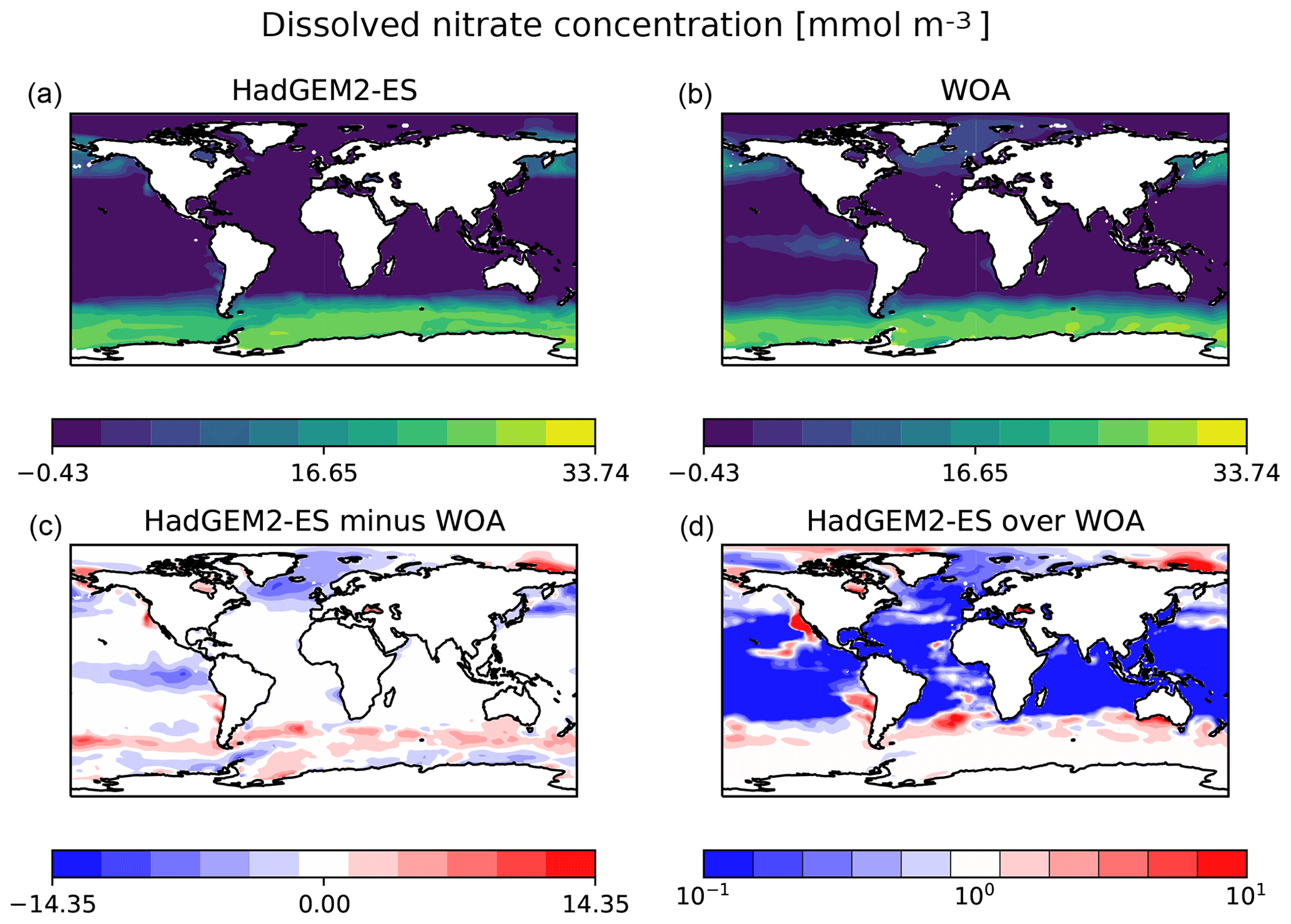
Figure 38The surface dissolved nitrate concentration in the CMIP5 HadGEM2-ES model compared against the World Ocean Atlas 2013 nitrate. Panels (a) and (b) show the surface fields; (c) and (d) show the difference and the quotient between the two datasets. Produced with recipe_ocean_bgc.yml; see details in Sect. 3.5.3.
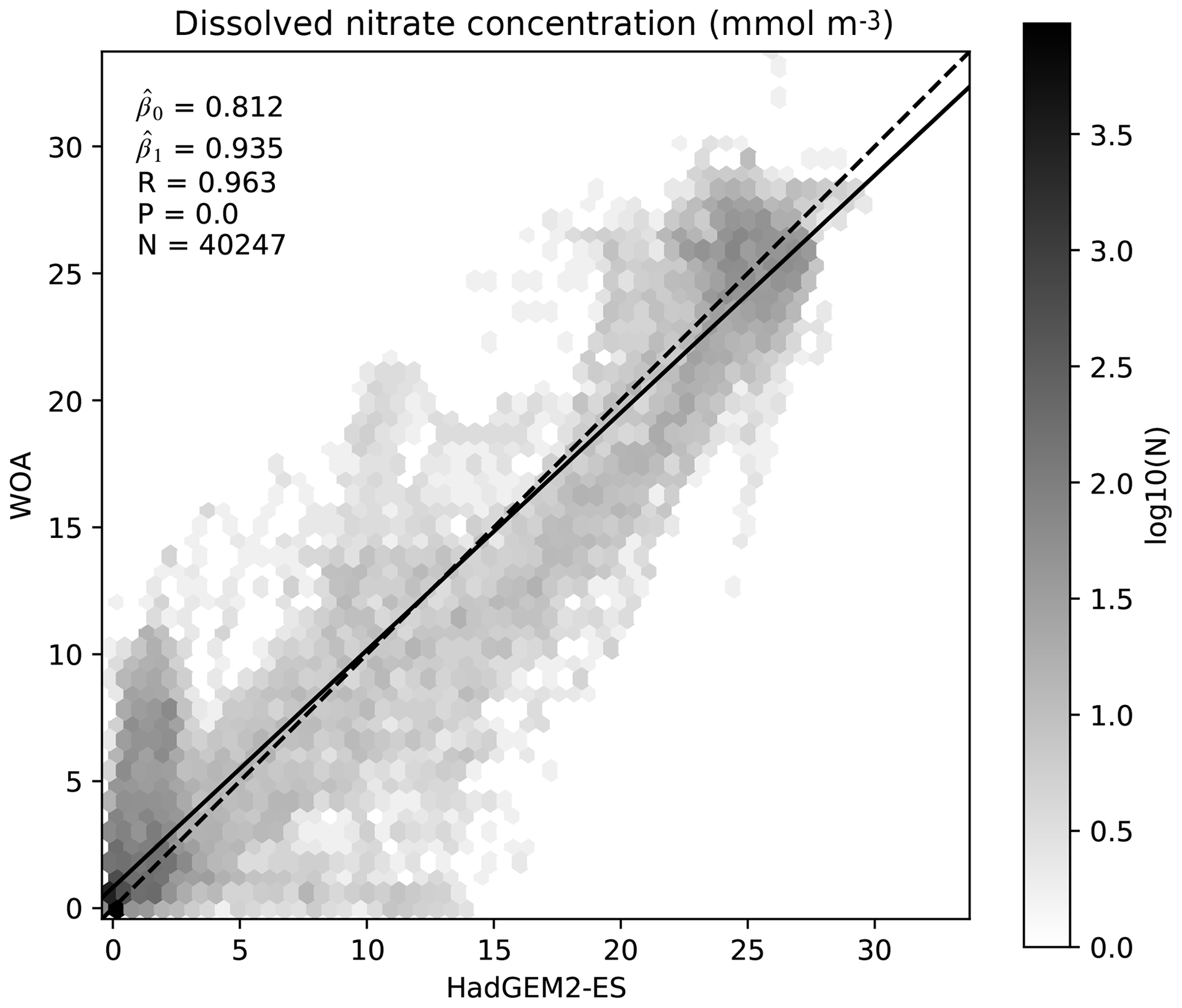
Figure 39The surface dissolved nitrate concentration in the CMIP5 HadGEM2-ES model (log 10(N)) compared against the World Ocean Atlas 2013 nitrate. This figure shows the paired model and observational datasets. A linear regression line of best fit is shown as a black line. A dashed line indicates the 1 : 1 line. The result of a linear regression are shown in the top left corner of the figure, where is the intersect, β1 is the slope, R is the correlation, P is the P value, and N is the number of data point pairs. Produced with recipe_ocean_bgc.yml; see details in Sect. 3.5.3.
Figure 40 shows the global average depth profile of the dissolved nitrate concentration in the HadGEM2-ES model and against the World Ocean Atlas dataset. The colour scale indicates the annual average, although in this specific case there is little observed interannual variability so the annual averages are closely overlaid. Nevertheless, this class of figure can be useful to evaluate biases between model and observations over the entire depth profile of the ocean and can also be used to identify long-term changes in the vertical structure of the ocean models. This figure shows that while the model and the observations both have a similar overall depth structure, the model is not able to produce the observed maximum nitrate concentration at approximately 1000 m depth and overestimates the nitrate concentration deeper in the water column. A multiple-panel comparison of satellite-derived observations for marine primary production against 16 CMIP5 models over the period 1995–2004 is shown in Fig. 41. Both observation and model data are regridded to a regular horizontal grid and differences are then computed. Systematic biases characterize all models mainly in the equatorial Pacific and Antarctic regions, in some cases with the opposite sign, and coastal ocean productivity is generally underestimated with major deviations in the equatorial zone.
3.5.4 Stratospheric temperature and trace species influencing stratospheric ozone chemistry
The recipe_eyring06jgr.yml has been ported in ESMValTool v2.0 from the CCMVal-Diag tool described by Gettelman et al. (2012) to evaluate a coupled chemistry–climate model (CCM) based on a set of core processes relevant for stratospheric ozone concentrations, centred around four main categories (radiation, dynamics, transport, and stratospheric chemistry). Each process is associated with one or more model diagnostics and with relevant observational datasets that can be used for the model evaluation (Eyring et al., 2006, 2005).
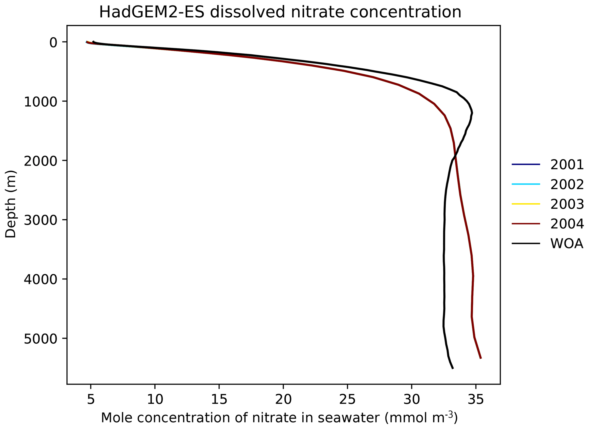
Figure 40The global area-weighted average depth profile of the dissolved nitrate concentration in the CMIP5 HadGEM2-ES model and against the World Ocean Atlas 2013. Produced with recipe_ocean_bgc.yml; see details in Sect. 3.5.3.
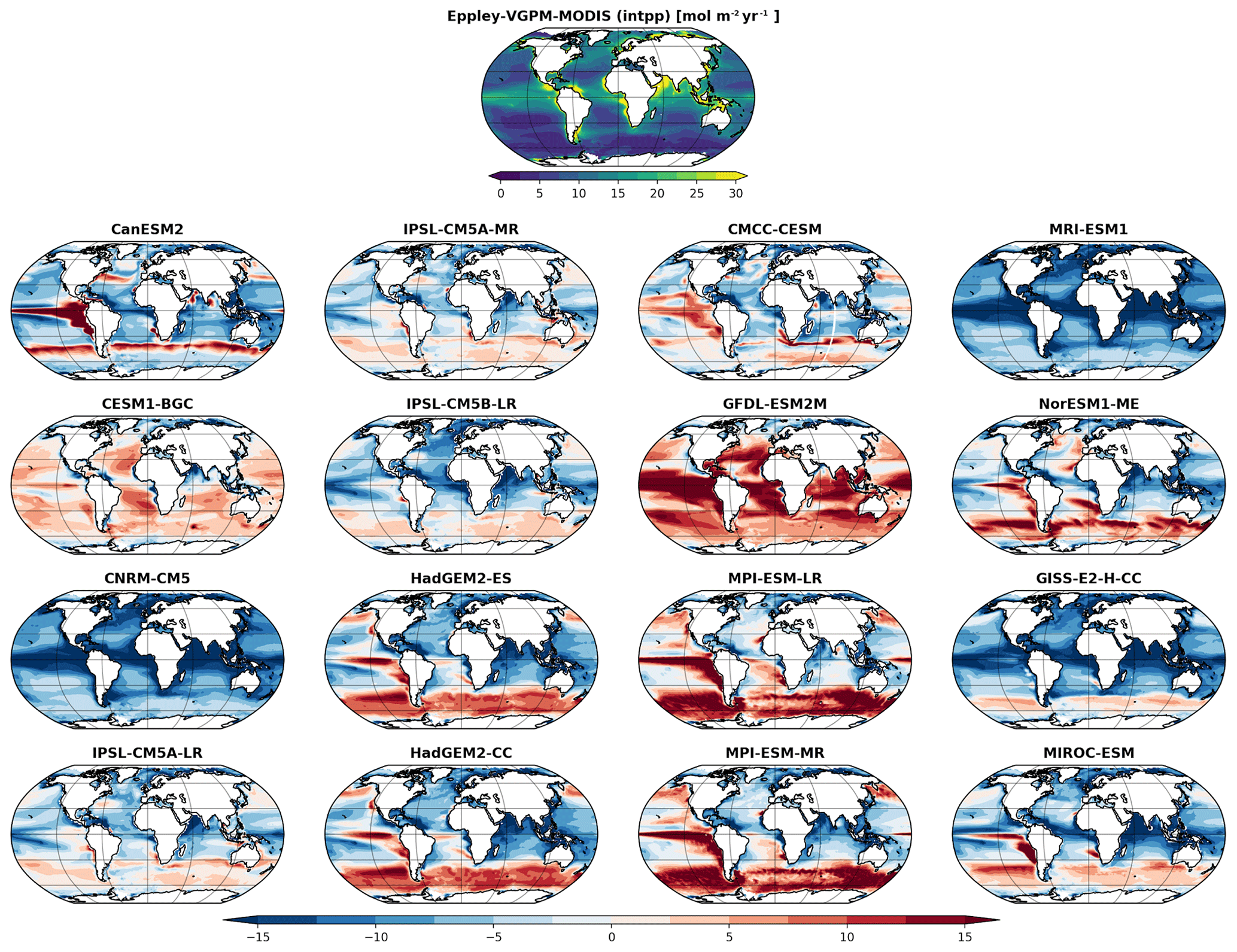
Figure 41Global maps of marine primary production as carbon (mol m−2 yr−1) estimated from MODIS satellite data using the Eppley VGPM algorithm (top panel) and differences computed for 16 CMIP5 models with data averaged over the period 1995–2004. See Sect. 3.5.3 for details on recipe_ocean_bgc.yml.
Since most of the chemical reactions determining ozone distribution in the stratosphere depend on temperature, recipe_eyring06jgr.yml allows the comparison of modelled stratospheric temperature with observations in terms of climatological mean, variability, and trends (Fig. 42). High-latitude temperatures in winter and spring are particularly important for correctly modelling polar ozone depletion induced by polar stratospheric clouds. In the middle stratosphere there are large variations between the analyses and most models, with no clear bias direction, whereas the temperature bias in the troposphere between analyses and models is somewhat smaller but is negative around 200 hPa in most models. The upper stratosphere is only available for a few models, and while for most of the seasons shown the agreement is relatively good, the spread between analyses and models is very large for the Antarctic polar regions in JJA. The recipe_eyring06jgr.yml evaluates the main features of the atmospheric transport by examining the distribution of long-lived traces (such as methane or N2O), the vertical propagation of the annual cycle of water vapour (“tape recorder”), and the mean age of air. Due to its important role in driving stratospheric ozone depletion, especially in the polar regions, this recipe includes the vertical distribution and temporal evolution of modelled chlorine (Cly). It also assesses the capability of the models to simulate realistic ozone vertical distributions (Fig. 43) and total ozone annual cycle. Ozone is clearly overestimated by most models, compared to the observations, in the northern high latitudes between 50 and 10 hPa, which also becomes apparent in the climatological zonal mean at 50 hPa. Southern high latitudes are slightly better represented in the models at 50 hPa with a more general spread around the observations, but at lower pressure levels an overestimation of ozone compared to the observations becomes apparent in some models.
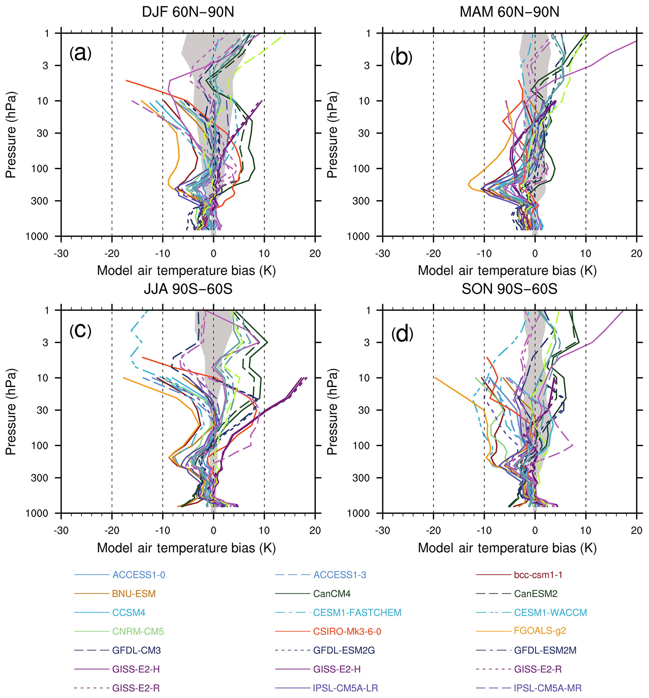
Figure 42CCM climatological mean temperature biases for (a, b) 60–90∘ N and (c, d) 60–90∘ S for the (a, c) winter and (b, d) spring seasons for the period 1980 to 1999. Biases are calculated relative to ERA-40 reanalyses. The grey area shows ERA-40 plus and minus 1 standard deviation about the climatological mean. Similar to Fig. 1 of Eyring et al. (2006) and produced with the recipe_eyring06jgr.yml. See details in Sect. 3.5.4.
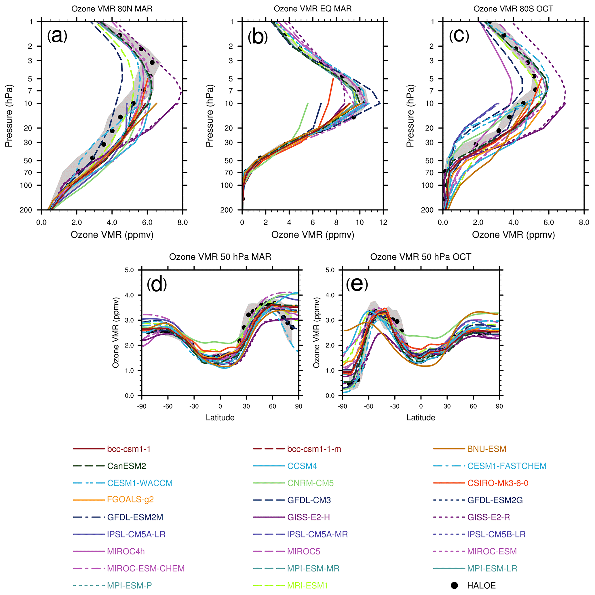
Figure 43Climatological zonal mean ozone mixing ratios from the CMIP5 simulations and HALOE in parts per million by volume. Vertical profiles at (a) 80∘ N in March, (b) 0 in March, and (c) 80∘ S in October. Latitudinal profiles at 50 hPa in (d) March and (e) October. The grey area shows HALOE plus and minus 1 standard deviation (s) about the climatological zonal mean. Similar to Fig. 5 of Eyring et al. (2006) and produced with the recipe_eyring06jgr.yml. See details in Sect. 3.5.4.
4.1 Running ESMValTool alongside the ESGF
An important goal for CMIP6 was to establish a system that allows for routine model evaluation alongside the ESGF directly after the model output is published to the CMIP archive (Eyring et al., 2016a, b, 2019). With the release of ESMValTool v2.0, this was reached through a semi-automatic execution of ESMValTool at the Deutsches Klimarechenzentrum (DKRZ) on CMIP6 data published to the ESGF. This is supported by the following components: (1) a locally hosted CMIP6 replica data pool, (2) an automatic CMIP6 data replication process, embracing ESMValTool data needs as replication priorities, and (3) a query mechanism to inform ESMValTool of the availability of new data in the data pool. Based on these components both regularly scheduled ESMValTool executions as well as executions triggered by the availability of new data can be realized. At the moment, the automatic regular execution is implemented. The replica pool is hosted as part of the parallel Lustre HPC (high-performance computing) file system at DKRZ and associated with a dedicated data project which is supervised by a panel deciding on CMIP6 data storage priorities. However, rapid data replication from ESGF to the local replica tool remains an issue that requires further work; see also the discussion in Eyring et al. (2016b).
ESMValTool data needs are managed in a GitHub repository and automatically integrated into the Synda tool (http://prodiguer.github.io/synda/, last access: 13 July 2020) based CMIP6 replication pipeline at DKRZ. The content of the data pool is regularly indexed, thus providing a high-performance query mechanism on locally available data. This index is used to automatically update several recipes with all available CMIP6 models. If new model output has been published to the ESGF, an ESMValTool execution is triggered and new plots are created. The results produced by ESMValTool are automatically copied to a result cache which is used by the result browser (see next section).
4.2 ESMValTool result browser at DKRZ
The ESMValTool result browser has been set up at http://cmip-esmvaltool.dkrz.de/ (last access: 13 July 2020). The ESMValTool results are visualized with the Freie University Evaluation System (FREVA). FREVA provides efficient and comprehensive access to the evaluation results and datasets. The application system is developed as an easy to use low-end application minimizing technical requirements for users and tool developers. Initially this website shows CMIP5 results that are already published. Newly produced results for CMIP6 are initially watermarked and are only made available without a watermark once quality control has taken place and related papers have been written. This strategy has been supported, encouraged, and approved by the WCRP Working Group of Coupled Modelling (WGCM). The result browser includes a search function that allows us to sort by ESMValTool recipes, projects, CMIP6 realms, scientific themes, domain, plot type, applied statistics, references, variables, datasets (including models, multi-model mean, and median and observations), and results. Each figure includes a caption, which is displayed alongside with the figure, and the corresponding metadata. These metadata include the ESMValTool configuration used to perform the analysis and draw the plot, software versions, date of production, input data, program output, notes, and results. In order to get a quick overview, a summary of the ESMValTool configuration used to create a given plot is also available. This summary includes the recipe name, variables, and models used as well as the name of the diagnostic script run and the exact version of ESMValTool (corresponds to the release tag on GitHub) used as basic information to reproduce a plot. Full provenance information providing all details on the figure creation such as the version of the input files and preprocessing steps applied is stored in the metadata of the figure file itself and can be retrieved by downloading the figure and reading the Exif header of the image file.
ESMValTool is a community diagnostics and performance metrics tool specifically targeted at facilitating and enhancing a comprehensive evaluation of ESMs participating in CMIP. Since the first ESMValTool release in 2016 (v1.0, Eyring et al., 2016c), substantial technical improvements have been made by a continuously growing developer community and additional diagnostics have been added. The tool is now developed by more than 40 institutions as open-source code on a Github repository (https://github.com/ESMValGroup, last access: 13 July 2020).
This paper is part of a series of publications that describe the release of ESMValTool version 2.0 (v2.0). One of the main structural changes compared to v1.0 is the separation of the tool into ESMValCore and a diagnostic part. ESMValCore is an easy-to-install, well-documented Python package that provides the core functionalities to perform common preprocessing operations and writes the output from models and observations to netCDF files (Righi et al., 2020). These preprocessed output files are then read by the diagnostic part that includes tailored diagnostics and performance metrics for specific scientific applications that are called by recipes. These recipes reproduce sets of diagnostics or performance metrics that have demonstrated their importance in ESM evaluation in the peer-reviewed literature.
This paper describes recipes for the evaluation of large-scale diagnostics in ESMValTool v2.0. It focuses on those diagnostics that were not part of the first major release of the tool (Eyring et al., 2016c) and includes (1) integrative measures of model performance, as well as diagnostics for the evaluation of processes in (2) the atmosphere, (3) the ocean and cryosphere, (4) land, and (5) biogeochemistry. Recipes for extreme events and in support of regional model evaluation are described by Weigel et al. (2020) and recipes for emergent constraints and model weighting by Lauer et al. (2020).
Compared to ESMValTool v1.0, the integrative measures of model performance have been expanded with additional atmospheric variables as well as new variables from the ocean, sea ice, and land (extending Fig. 9.7 of Flato et al., 2013). In addition, the centred pattern correlation that allows the quantification of progress between different ensembles of CMIP models for multiple variables (extending Fig. 9.6 of Flato et al., 2013) and the single-model performance index proposed by Reichler and Kim (2008) that allows an overall assessment of model performance have been added. For the purpose of model development it is important to look at many different metrics. AutoAssess, which is developed by the UK Met Office, therefore includes a mix of top–down metrics evaluating key model output variables and bottom–up process-oriented metrics. AutoAssess includes 11 thematic areas, which will all be implemented in ESMValTool, but in v2.0, as a technical demonstration, only the area for the stratosphere was implemented.
Table 2Overview of CMIP5 models used in the figures shown in this paper alongside with a reference.
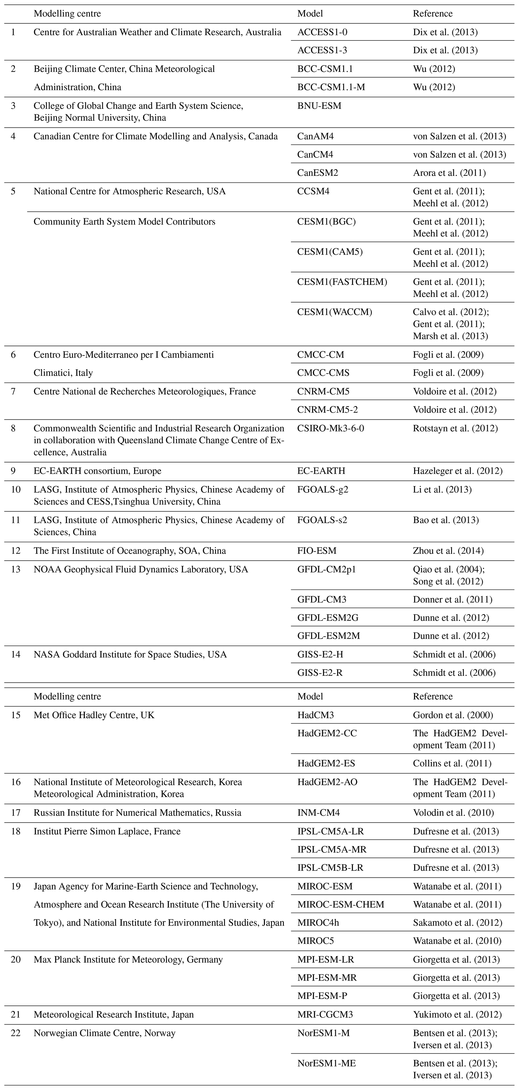
For the evaluation of processes in the atmosphere, the recipe to calculate multi-model averages (e.g. for surface temperature and precipitation) now not only includes absolute values but also the mean root-mean-square error of the seasonal cycle compared to observations. The time series of the anomalies in annual and global mean surface temperature with the models being subsampled as in the observations from HadCRUT4 is also included. In addition, a recipe for the evaluation of the precipitation quantile bias has been added. For atmospheric dynamics, recipes to evaluate stratosphere–troposphere coupling and atmospheric blocking indices have been included. A new diagnostic tool for the evaluation of the water, energy, and entropy budgets in climate models (TheDiaTo (v1.0), Lembo et al., 2019) has been newly implemented, while the NCAR Climate Variability Diagnostic Package (Phillips et al., 2014), already available in v1.0, has been updated in ESMValTool v2.0 to its latest version. In addition, several other diagnostics to evaluate modes of variability as well as weather regimes calculated by the MiLES package (Davini, 2018) have been added.
To evaluate the broad behaviour of models for the global ocean, several diagnostics have been newly implemented, including diagnostics to evaluate the volume-weighted global average temperature anomaly, the AMOC, the Drake Passage Current, the global total flux of CO2 from the atmosphere into the ocean, and the global total integrated primary production from phytoplankton. A recipe to evaluate specifically the Southern Ocean following Russell et al. (2018) has been included, and for the Arctic Ocean, vertical ocean distributions (e.g. temperature and salinity) for different Arctic Ocean basins and a transect that follows the pathway of the Atlantic water can now be calculated. For sea ice, a recipe related to the evaluation of the negative sea ice growth–thickness feedback which includes the IFE as a process-based diagnostic (Massonnet et al., 2018b) and a recipe that can quantify the relationships between Arctic sea ice drift speed, concentration, and thickness (Docquier et al., 2017) have been added.
For the evaluation of land processes, satellite-derived land cover classes cannot directly be used for ESM vegetation evaluation because DGVMs use different concepts for vegetation representation, typically based on plant functional types. A recipe has therefore been added that maps the ESA CCI land cover classes to plant functional types as described by Poulter et al. (2015). It includes major land cover types (bare soil, crops, grass, shrubs, trees) similar to the evaluation study by Lauer et al. (2017). In addition, a recipe has been added that can be used to evaluate albedo changes associated with land cover transitions using the ESA CCI dataset of Duveiller et al. (2018a).
For the terrestrial biosphere, a recipe that allows the evaluation of the main climatic variables controlling both the spatial and temporal characteristics of the carbon cycle on three different timescales (long-term trends, interannual variability, and seasonal cycles) has been added following Anav et al. (2013). These key variables include surface land temperature, precipitation over land, sea surface temperatures, land–atmosphere and ocean–atmosphere fluxes, gross primary production, leaf area index, and carbon content in soil and vegetation. To evaluate the simulated land carbon stocks that integrate the land–atmosphere carbon exchange, a recipe to evaluate biases in ecosystem carbon turnover time, the time period that a carbon atom on average spends in land ecosystems, from assimilation through photosynthesis to its release back into the atmosphere (Carvalhais et al., 2014) has been added. For marine biogeochemistry, v2.0 now includes a recipe that allows a direct comparison of the models against observational data for several variables including temperature, salinity, oxygen, nitrate, phosphate, silicate, CO2 air–sea fluxes, chlorophyll a, and primary production. The point-to-point comparison of the model against the observational dataset is similar to De Mora et al. (2013). To evaluate stratospheric dynamics and chemistry a recipe based on a set of core processes relevant for stratospheric ozone concentrations, centred around four main categories (radiation, dynamics, transport, and stratospheric chemistry) has been added (Eyring et al., 2006). Overall these recipes together with those already included in v1.0 allow a broad characterization of the models for key variables (such as temperature and precipitation) on the large scale, but v2.0 also includes several process-oriented diagnostics.
With this release, for the first time in CMIP it is now possible to evaluate the models as soon as the output is published to the ESGF in a quasi-operational manner. To achieve this, ESMValTool has been fully integrated into the ESGF structure at DKRZ. The data from the ESGF are first copied to a local replica, and ESMValTool is then automatically executed alongside the ESGF as soon as new output arrives. An ESMValTool result browser has been set up that makes the evaluation results available to the wider community (http://cmip-esmvaltool.dkrz.de/, last access: 13 July 2020).
Another major advancement of ESMValTool v2.0 is that it provides full provenance and traceability (see Sect. 5.2 in Righi et al., 2020, for details). Provenance information, for example, includes technical information such as global attributes of all input netCDF files, preprocessor settings, diagnostic script settings, and software version numbers but also diagnostic script name and recipe authors, funding projects, references for citation purposes, as well as tags for categorizing the result plots into various scientific topics (like chemistry, dynamics, sea ice) realms (land, atmosphere, ocean, etc.) or the statistics applied (RMSE, anomaly, trend, climatology, etc.). This not only facilitates the sorting of the results in the ESMValTool result browser but also qualifies the tool for the use in studies or assessments where provenance and traceability is particularly important. The current approach to provenance and tags (i.e. what is reported) can be adjusted to international provenance standards as they become available.
These recent ESMValTool developments and their coupling to the ESGF results can now be exploited by global and regional ESM developers as well as by the data analysis and user communities, to better understand the large CMIP ensemble and to support data exploitation. In particular with the addition of provenance, the tool can also provide a valuable source for producing figures in national and international assessment reports (such as the IPCC climate assessments) to enhance the quality control, reproducibility, and traceability of the figures included.
The ESMValTool development community will further enhance the capabilities of the tool with the goal of taking climate model evaluation – together with other activities – to the next level (Eyring et al., 2019). Targeted technical enhancements will, for example, include the development of quick-look capabilities that allow users to monitor the simulations while they are running to help identify errors in the simulations early on, a further extension to the application to regional models so that a consistent evaluation between global and regional models can be provided, and distributed computing functionalities. In addition, the tool will be expanded with additional process-oriented diagnostics in various projects to further enhance comprehensive evaluation and analysis of the CMIP models.
ESMValTool v2.0 is released under the Apache License, VERSION 2.0. The latest release of ESMValTool v2.0 is publicly available on Zenodo at https://doi.org/10.5281/zenodo.3759523 (Andela et al., 2020a). The source code of the ESMValCore package, which is installed as a dependency of the ESMValTool v2.0, is also publicly available on Zenodo at https://doi.org/10.5281/zenodo.3952695 (Andela et al., 2020b). ESMValTool and ESMValCore are developed on the GitHub repositories available at https://github.com/ESMValGroup (last access: 13 July 2020).
CMIP5 data are available freely and publicly from the Earth System Grid Federation. Observations used in the evaluation are detailed in the various sections of the paper and listed in Table 1. They are not distributed with ESMValTool, which is restricted to the code as open-source software.
VE coordinated the ESMValTool v2.0 diagnostic effort and led the writing of the paper. LB, AL, MR, and MS coordinated the diagnostic implementation in ESMValTool v2.0. CE and SK helped with the coupling of ESMValTool v2.0 and CK with the visualization of the results in the ESMValTool result browser. All other co-authors contributed individual diagnostics to this release. All authors contributed to the text.
The authors declare that they have no conflict of interest.
We dedicate this paper to our great friend and colleague, Alexander Loew, who lost his life in a tragic traffic accident. Our thoughts are with his family and his department. The diagnostic development of ESMValTool v2.0 for this paper was supported by different projects with different scientific focuses, in particular by (1) the European Union's Horizon 2020 Framework Programme for Research and Innovation “Coordinated Research in Earth Systems and Climate: Experiments, kNowledge, Dissemination and Outreach (CRESCENDO)” project under grant agreement no. 641816, (2) the Copernicus Climate Change Service (C3S) ”Metrics and Access to Global Indices for Climate Projections (C3S-MAGIC)” project, (3) the European Union's Horizon 2020 Framework Programme for Research and Innovation “Advanced Prediction in Polar regions and beyond: Modelling, observing system design and LInkages associated with a Changing Arctic climate (APPLICATE)” project under grant agreement no. 727862, (4) the European Union's Horizon 2020 Framework Programme for Research and Innovation “PRocess-based climate sIMulation: AdVances in high-resolution modelling and European climate Risk Assessment (PRIMAVERA)” project under grant agreement no. 641727, (5) the Federal Ministry of Education and Research (BMBF) CMIP6-DICAD project, (6) the ESA Climate Change Initiative Climate Model User Group (ESA CCI CMUG), (7) the Helmholtz Society project “Advanced Earth System Model Evaluation for CMIP (EVal4CMIP)”, (8) project S1 (Diagnosis and Metrics in Climate Models) of the Collaborative Research Centre TRR 181 “Energy Transfer in Atmosphere and Ocean” funded by the Deutsche Forschungsgemeinschaft (DFG, German Research Foundation) project no. 274762653, and (9) the National Environmental Research Council (NERC) National Capability Science Multi-Centre (NCSMC) funding for the UK Earth System Modelling project (grant NE/N018036/1). In addition, we received technical support on the ESMValTool v2.0 development from the European Union's Horizon 2020 Framework Programme for Research and Innovation “Infrastructure for the European Network for Earth System Modelling (IS-ENES3)” project under grant agreement no. 824084. We acknowledge the World Climate Research Program's (WCRP's) Working Group on Coupled Modelling (WGCM), which is responsible for CMIP, and we thank the climate modelling groups listed in Table 2 for producing and making available their model output. We thank Mariano Mertens (DLR, Germany) for his helpful comments on a previous version and Michaela Langer (DLR, Germany) for her help with editing the paper. The computational resources of the Deutsches Klimarechenzentrum (DKRZ, Hamburg, Germany) were essential for developing and testing this new version and are kindly acknowledged.
This research has been supported by Horizon 2020 (grant nos. 641816, 727862, 641727, and 824084), the Copernicus Climate Change Service (C3S) (Metrics and Access to Global Indices for Climate Projections, MAGIC), the Helmholtz Association (Advanced Earth System Model Evaluation for CMIP, EVal4CMIP), the Deutsche Forschungsgemeinschaft (grant no. 274762653), the Federal Ministry of Education and Research (BMBF) (grant no. CMIP6-DICAD), and the European Space Agency (ESA Climate Change Initiative Climate Model User Group, ESA CCI CMUG).
The article processing charges for this open-access
publication were covered by a Research
Centre of the Helmholtz Association.
This paper was edited by Juan Antonio Añel and reviewed by two anonymous referees.
Achard, F., Beuchle, R., Mayaux, P., Stibig, H. J., Bodart, C., Brink, A., Carboni, S., Desclee, B., Donnay, F., Eva, H. D., Lupi, A., Rasi, R., Seliger, R., and Simonetti, D.: Determination of tropical deforestation rates and related carbon losses from 1990 to 2010, Glob. Change Biol., 20, 2540–2554, 2014.
Adler, R. F., Huffman, G. J., Chang, A., Ferraro, R., Xie, P.-P., Janowiak, J., Rudolf, B., Schneider, U., Curtis, S., and Bolvin, D.: The version-2 global precipitation climatology project (GPCP) monthly precipitation analysis (1979–present), J. Hydrometeorol., 4, 1147–1167, 2003.
Alkama, R. and Cescatti, A.: Biophysical climate impacts of recent changes in global forest cover, Science, 351, 600–604, 2016.
Ambaum, M. H.: Thermal physics of the atmosphere, John Wiley & Sons, 2010.
Anav, A., Friedlingstein, P., Kidston, M., Bopp, L., Ciais, P., Cox, P., Jones, C., Jung, M., Myneni, R., and Zhu, Z.: Evaluating the Land and Ocean Components of the Global Carbon Cycle in the CMIP5 Earth System Models, J. Climate, 26, 6801–6843, 2013.
Andela, B., Brötz, B., de Mora, L., Drost, N., Eyring, V., Koldunov,N., Lauer, A., Mueller, B., Predoi, V., Righi, M., Schlund, M.,Vegas-Regidor, J., Zimmermann, K., Adeniyi, K., Amarjiit, P.,Arnone, E., Bellprat, O., Berg, P., Bock, L., Caron, L.-P., Carval-hais, N., Cionni, I., Cortesi, N., Corti, S., Crezee, B., Davin, E.L., Davini, P., Deser, C., Diblen, F., Docquier, D., Dreyer, L., Ehbrecht, C., Earnshaw, P., Gier, B., Gonzalez-Reviriego, N., Goodman, P., Hagemann, S., von Hardenberg, J., Hassler, B., Hunter, A., Kadow, C., Kindermann, S., Koirala, S., Lledó, L.,Lejeune, Q., Lembo, V., Little, B., Loosveldt-Tomas, S., Lorenz, R., Lovato, T., Lucarini, V., Massonnet, F., Mohr, C. W., Pérez-Zanón, N., Phillips, A., Russell, J., Sandstad, M., Sellar, A., Senftleben, D., Serva, F., Sillmann, J., Stacke, T., Swaminathan, R., Torralba, V., and Weigel, K.: ESMValTool (Version v2.0.0b4), Zenodo, https://doi.org/10.5281/zenodo.3759523, 2020a.
Andela, B., Brötz, B., de Mora, L., Drost, N., Eyring, V., Koldunov, N., Lauer, A., Predoi, V., Righi, M., Schlund, M., Vegas Regidor, J., Zimmermann, K., Bock, L., Diblen, F., Dreyer, L., Earnshaw, P., Hassler, B., Little, B., and Loosveldt-Tomas, S.: ESMValCore (Version v2.0.0), Zenodo, https://doi.org/10.5281/zenodo.3952695, 2020b.
Arora, V. K., Boer, G. J., Friedlingstein, P., Eby, M., Jones, C. D., Christian, J. R., Bonan, G., Bopp, L., Brovkin, V., Cadule, P., Hajima, T., Ilyina, T., Lindsay, K., Tjiputra, J. F., and Wu, T.: Carbon-Concentration and Carbon-Climate Feedbacks in CMIP5 Earth System Models, J. Climate, 26, 5289–5314, 2013.
Arora, V. K., Scinocca, J. F., Boer, G. J., Christian, J. R., Denman, K. L., Flato, G. M., Kharin, V. V., Lee, W. G., and Merryfield, W. J.: Carbon emission limits required to satisfy future representative concentration pathways of greenhouse gases, Geophys. Res. Lett., 38, L05805, https://doi.org/10.1029/2010GL046270, 2011.
Aumann, H. H., Chahine, M. T., Gautier, C., Goldberg, M. D., Kalnay, E., McMillin, L. M., Revercomb, H., Rosenkranz, P. W., Smith, W. L., and Staelin, D. H.: AIRS/AMSU/HSB on the Aqua mission: Design, science objectives, data products, and processing systems, IEEE T. Geosci. Remote, 41, 253–264, 2003.
Balaji, V., Taylor, K. E., Juckes, M., Lawrence, B. N., Durack, P. J., Lautenschlager, M., Blanton, C., Cinquini, L., Denvil, S., Elkington, M., Guglielmo, F., Guilyardi, E., Hassell, D., Kharin, S., Kindermann, S., Nikonov, S., Radhakrishnan, A., Stockhause, M., Weigel, T., and Williams, D.: Requirements for a global data infrastructure in support of CMIP6, Geosci. Model Dev., 11, 3659–3680, https://doi.org/10.5194/gmd-11-3659-2018, 2018.
Baldwin, M. P. and Dunkerton, T. J.: Stratospheric harbingers of anomalous weather regimes, Science, 294, 581–584, 2001.
Baldwin, M. P. and Thompson, D. W. J.: A critical comparison of stratosphere–troposphere coupling indices, Q. J. Roy. Meteor. Soc., 135, 1661–1672, 2009.
Bao, Q., Lin, P., Zhou, T., Liu, Y., Yu, Y., Wu, G., He, B., He, J., Li, L., Li, J., Li, Y., Liu, H., Qiao, F., Song, Z., Wang, B., Wang, J., Wang, P., Wang, X., Wang, Z., Wu, B., Wu, T., Xu, Y., Yu, H., Zhao, W., Zheng, W., and Zhou, L.: The Flexible Global Ocean-Atmosphere-Land system model, Spectral Version 2: FGOALS-s2, Adv. Atmos. Sci., 30, 561–576, 2013.
Barriopedro, D., García-Herrera, R., and Trigo, R. M.: Application of blocking diagnosis methods to general circulation models. Part I: A novel detection scheme, Clim. Dynam., 35, 1373–1391, 2010.
Behrenfeld, M. J. and Falkowski, P. G.: Photosynthetic rates derived from satellite-based chlorophyll concentration, Limnol. Oceanogr., 42, 1–20, 1997.
Bengtsson, L. and Hodges, K. I.: Can an ensemble climate simulation be used to separate climate change signals from internal unforced variability?, Clim. Dynam., 52, 3553–3573, 2019.
Bentsen, M., Bethke, I., Debernard, J. B., Iversen, T., Kirkevåg, A., Seland, Ø., Drange, H., Roelandt, C., Seierstad, I. A., Hoose, C., and Kristjánsson, J. E.: The Norwegian Earth System Model, NorESM1-M – Part 1: Description and basic evaluation of the physical climate, Geosci. Model Dev., 6, 687–720, https://doi.org/10.5194/gmd-6-687-2013, 2013.
Bodeker, G. E., Shiona, H., and Eskes, H.: Indicators of Antarctic ozone depletion, Atmos. Chem. Phys., 5, 2603–2615, https://doi.org/10.5194/acp-5-2603-2005, 2005.
Boisier, J. P., de Noblet-Ducoudré, N., Pitman, A. J., Cruz, F. T., Delire, C., van den Hurk, B. J. J. M., van der Molen, M. K., Müller, C., and Voldoire, A.: Attributing the impacts of land-cover changes in temperate regions on surface temperature and heat fluxes to specific causes: Results from the first LUCID set of simulations, J. Geophys. Res., 117, D12116, https://doi.org/10.1029/2011JD017106, 2012.
Bonan, G.: Forests and climate change: forcings, feedbacks, and the climate benefits of forests, Science, 320, 1444–1449, 2008.
Brovkin, V., Boysen, L., Raddatz, T., Gayler, V., Loew, A., and Claussen, M.: Evaluation of vegetation cover and land-surface albedo in MPI-ESM CMIP5 simulations, J. Adv. Model. Earth Sy., 5, 48–57, 2013.
Buitenhuis, E. T., Hashioka, T., and Le Quéré, C.: Combined constraints on global ocean primary production using observations and models, Global Biogeochem. Cy., 27, 847–858, 2013.
Calvo, N., Garcia, R. R., Marsh, D. R., Mills, M. J., Kinnison, D. E., and Young, P. J.: Reconciling modeled and observed temperature trends over Antarctica, Geophys. Res. Lett., 39, L16803, https://doi.org/10.1029/2012GL052526, 2012.
Carissimo, B., Oort, A., and Vonder Haar, T.: Estimating the meridional energy transports in the atmosphere and ocean, J. Phys. Oceanogr., 15, 82–91, 1985.
Carvalhais, N., Forkel, M., Khomik, M., Bellarby, J., Jung, M., Migliavacca, M., Mu, M., Saatchi, S., Santoro, M., Thurner, M., Weber, U., Ahrens, B., Beer, C., Cescatti, A., Randerson, J. T., and Reichstein, M.: Global covariation of carbon turnover times with climate in terrestrial ecosystems, Nature, 514, 213–217, 2014.
Cassou, C., Terray, L., and Phillips, A. S.: Tropical Atlantic influence on European heat waves, J. Climate, 18, 2805–2811, 2005.
Charlton-Perez, A. J., Baldwin, M. P., Birner, T., Black, R. X., Butler, A. H., Calvo, N., Davis, N. A., Gerber, E. P., Gillett, N., and Hardiman, S.: On the lack of stratospheric dynamical variability in low-top versions of the CMIP5 models, J. Geophys. Res., 118, 2494–2505, 2013.
Cheng, W., Chiang, J. C., and Zhang, D.: Atlantic meridional overturning circulation (AMOC) in CMIP5 models: RCP and historical simulations, J. Climate, 26, 7187–7197, 2013.
Collins, W. J., Bellouin, N., Doutriaux-Boucher, M., Gedney, N., Halloran, P., Hinton, T., Hughes, J., Jones, C. D., Joshi, M., Liddicoat, S., Martin, G., O'Connor, F., Rae, J., Senior, C., Sitch, S., Totterdell, I., Wiltshire, A., and Woodward, S.: Development and evaluation of an Earth-System model – HadGEM2, Geosci. Model Dev., 4, 1051–1075, https://doi.org/10.5194/gmd-4-1051-2011, 2011.
Coumou, D. and Rahmstorf, S.: A decade of weather extremes, Nat. Clim. Change, 2, 491–496, 2012.
Cox, P. M., Pearson, D., Booth, B. B., Friedlingstein, P., Huntingford, C., Jones, C. D., and Luke, C. M.: Sensitivity of tropical carbon to climate change constrained by carbon dioxide variability, Nature, 494, 341–344, 2013.
Danabasoglu, G., Bates, S. C., Briegleb, B. P., Jayne, S. R., Jochum, M., Large, W. G., Peacock, S., and Yeager, S. G.: The CCSM4 ocean component, J. Climate, 25, 1361–1389, 2012.
Davin, E. L., Rechid, D., Breil, M., Cardoso, R. M., Coppola, E., Hoffmann, P., Jach, L. L., Katragkou, E., de Noblet-Ducoudré, N., Radtke, K., Raffa, M., Soares, P. M. M., Sofiadis, G., Strada, S., Strandberg, G., Tölle, M. H., Warrach-Sagi, K., and Wulfmeyer, V.: Biogeophysical impacts of forestation in Europe: first results from the LUCAS (Land Use and Climate Across Scales) regional climate model intercomparison, Earth Syst. Dynam., 11, 183–200, https://doi.org/10.5194/esd-11-183-2020, 2020.
Davini, P.: MiLES – Mid Latitude Evaluation System (Version v0.51), Zenodo, https://doi.org/10.5281/zenodo.1237838, 2018.
Davini, P. and Cagnazzo, C.: On the misinterpretation of the North Atlantic Oscillation in CMIP5 models, Clim. Dynam., 43, 1497–1511, 2013.
Davini, P., Cagnazzo, C., Gualdi, S., and Navarra, A.: Bidimensional diagnostics, variability, and trends of Northern Hemisphere blocking, J. Climate, 25, 6496–6509, 2012.
Davini, P. and D'Andrea, F.: Northern Hemisphere atmospheric blocking representation in global climate models: Twenty years of improvements?, J. Climate, 29, 8823–8840, 2016.
Dawson, A., Palmer, T., and Corti, S.: Simulating regime structures in weather and climate prediction models, Geophys. Res. Lett., 39, L21805, https://doi.org/10.1029/2012GL053284, 2012.
de Mora, L., Butenschön, M., and Allen, J. I.: How should sparse marine in situ measurements be compared to a continuous model: an example, Geosci. Model Dev., 6, 533–548, https://doi.org/10.5194/gmd-6-533-2013, 2013.
de Noblet-Ducoudré, N., Boisier, J.-P., Pitman, A., Bonan, G., Brovkin, V., Cruz, F., Delire, C., Gayler, V., Van den Hurk, B., and Lawrence, P.: Determining robust impacts of land-use-induced land cover changes on surface climate over North America and Eurasia: results from the first set of LUCID experiments, J. Climate, 25, 3261–3281, 2012.
Dee, D. P., Uppala, S. M., Simmons, A. J., Berrisford, P., Poli, P., Kobayashi, S., Andrae, U., Balmaseda, M. A., Balsamo, G., Bauer, P., Bechtold, P., Beljaars, A. C. M., van de Berg, I., Biblot, J., Bormann, N., Delsol, C., Dragani, R., Fuentes, M., Greer, A. J., Haimberger, L., Healy, S. B., Hersbach, H., Holm, E. V., Isaksen, L., Kallberg, P., Kohler, M., Matricardi, M., McNally, A. P., Mong-Sanz, B. M., Morcette, J.-J., Park, B.-K., Peubey, C., de Rosnay, P., Tavolato, C., Thepaut, J. N., and Vitart, F.: The ERA-Interim reanalysis: Configuration and performance of the data assimilation system, Q. J. Roy. Meteorol. Soc., 137, 553–597, https://doi.org/10.1002/qj.828, 2011.
Defourny, P., Boettcher, M., Bontemps, S., Kirches, G., Krueger, O., Lamarche, C., Lembrée, C., Radoux, J., and Verheggen, A.: Algorithm theoretical basis document for land cover climate change initiative, Technical report, European Space Agency, 2014.
Defourny, P., Boettcher, M., Bontemps, S., Kirches, G., Lamarche, C., Peters, M., Santoro, M., and Schlerf, M.: Land cover cci Product user guide version 2, Technical report, European Space Agency, 2016.
Deser, C., Alexander, M. A., Xie, S. P., and Phillips, A. S.: Sea Surface Temperature Variability: Patterns and Mechanisms, Ann. Rev. Mar. Sci., 2, 115–143, 2010.
Deser, C., Knutti, R., Solomon, S., and Phillips, A. S.: Communication of the role of natural variability in future North American climate, Nat. Clim. Change, 2, 77–779, 2012.
Deser, C., Phillips, A. S., Alexander, M. A., and Smoliak, B. V.: Projecting North American Climate over the Next 50 Years: Uncertainty due to Internal Variability, J. Climate, 27, 2271–2296, 2014.
Deser, C., Simpson, I. R., McKinnon, K. A., and Phillips, A. S.: The Northern Hemisphere extratropical atmospheric circulation response to ENSO: How well do we know it and how do we evaluate models accordingly?, J. Climate, 30, 5059–5082, 2017.
Di Biagio, V., Calmanti, S., Dell'Aquila, A., and Ruti, P. M.: Northern Hemisphere winter midlatitude atmospheric variability in CMIP5 models, Geophys. Res. Lett., 41, 1277–1282, 2014.
Dix, M., Vohralik, P., Bi, D., Rashid, H. A., Marsland, S., O'Farrell, S., Uotila, P., Hirst, A. C., Kowalczyk, E. A., Sullivan, A., Yan, H., Franklin, C., Sun, Z., Watterson, I., Collier, M., Noonan, J., Stevens, L., Uhe, P., and Puri, K.: The ACCESS Coupled Model: Documentation of core CMIP5 simulations and initial results, Aust. Met. Oceanog. J., 63, 41–64, 2013.
Docquier, D., Massonnet, F., Barthélemy, A., Tandon, N. F., Lecomte, O., and Fichefet, T.: Relationships between Arctic sea ice drift and strength modelled by NEMO-LIM3.6, The Cryosphere, 11, 2829–2846, https://doi.org/10.5194/tc-11-2829-2017, 2017.
Donner, L. J., Wyman, B. L., Hemler, R. S., Horowitz, L. W., Ming, Y., Zhao, M., Golaz, J. C., Ginoux, P., Lin, S. J., Schwarzkopf, M. D., Austin, J., Alaka, G., Cooke, W. F., Delworth, T. L., Freidenreich, S. M., Gordon, C. T., Griffies, S. M., Held, I. M., Hurlin, W. J., Klein, S. A., Knutson, T. R., Langenhorst, A. R., Lee, H. C., Lin, Y. L., Magi, B. I., Malyshev, S. L., Milly, P. C. D., Naik, V., Nath, M. J., Pincus, R., Ploshay, J. J., Ramaswamy, V., Seman, C. J., Shevliakova, E., Sirutis, J. J., Stern, W. F., Stouffer, R. J., Wilson, R. J., Winton, M., Wittenberg, A. T., and Zeng, F. R.: The Dynamical Core, Physical Parameterizations, and Basic Simulation Characteristics of the Atmospheric Component AM3 of the GFDL Global Coupled Model CM3, J. Climate, 24, 3484–3519, 2011.
Donohue, K., Tracey, K., Watts, D., Chidichimo, M. P., and Chereskin, T.: Mean antarctic circumpolar current transport measured in drake passage, Geophys. Res. Lett., 43, 11760–11767, 2016.
Dufresne, J. L., Foujols, M. A., Denvil, S., Caubel, A., Marti, O., Aumont, O., Balkanski, Y., Bekki, S., Bellenger, H., Benshila, R., Bony, S., Bopp, L., Braconnot, P., Brockmann, P., Cadule, P., Cheruy, F., Codron, F., Cozic, A., Cugnet, D., Noblet, N., Duvel, J. P., Ethé, C., Fairhead, L., Fichefet, T., Flavoni, S., Friedlingstein, P., Grandpeix, J. Y., Guez, L., Guilyardi, E., Hauglustaine, D., Hourdin, F., Idelkadi, A., Ghattas, J., Joussaume, S., Kageyama, M., Krinner, G., Labetoulle, S., Lahellec, A., Lefebvre, M. P., Lefevre, F., Levy, C., Li, Z. X., Lloyd, J., Lott, F., Madec, G., Mancip, M., Marchand, M., Masson, S., Meurdesoif, Y., Mignot, J., Musat, I., Parouty, S., Polcher, J., Rio, C., Schulz, M., Swingedouw, D., Szopa, S., Talandier, C., Terray, P., Viovy, N., and Vuichard, N.: Climate change projections using the IPSL-CM5 Earth System Model: from CMIP3 to CMIP5, Clim. Dynam., 40, 2123–2165, https://doi.org/10.1007/s00382-012-1636-1, 2013.
Dunne, J. P., John, J. G., Adcroft, A. J., Griffies, S. M., Hallberg, R. W., Shevliakova, E., Stouffer, R. J., Cooke, W., Dunne, K. A., Harrison, M. J., Krasting, J. P., Malyshev, S. L., Milly, P. C. D., Phillipps, P. J., Sentman, L. T., Samuels, B. L., Spelman, M. J., Winton, M., Wittenberg, A. T., and Zadeh, N.: GFDL's ESM2 Global Coupled Climate-Carbon Earth System Models. Part I: Physical Formulation and Baseline Simulation Characteristics, J. Climate, 25, 6646–6665, 2012.
Duveiller, G., Hooker, J., and Cescatti, A.: A dataset mapping the potential biophysical effects of vegetation cover change, Sci. Data, 5, 180014, https://doi.org/10.1038/sdata.2018.14, 2018a.
Duveiller, G., Hooker, J., and Cescatti, A.: The mark of vegetation change on Earth's surface energy balance, Nature communications, 9, 679, https://doi.org/10.1038/s41467-017-02810-8, 2018b.
Ellison, D., N. Futter, M., and Bishop, K.: On the forest cover–water yield debate: from demand-to supply-side thinking, Glob. Change Biol., 18, 806–820, 2012.
Exarchou, E., Kuhlbrodt, T., Gregory, J. M., and Smith, R. S.: Ocean heat uptake processes: a model intercomparison, J. Climate, 28, 887–908, 2015.
Eyring, V., Harris, N. R. P., Rex, M., Shepherd, T. G., Fahey, D. W., Amanatidis, G. T., Austin, J., Chipperfield, M. P., Dameris, M., Forster, P. M. D. F., Gettelman, A., Graf, H. F., Nagashima, T., Newman, P. A., Pawson, S., Prather, M. J., Pyle, J. A., Salawitch, R. J., Santer, B. D., and Waugh, D. W.: A Strategy for Process-Oriented Validation of Coupled Chemistry–Climate Models, B. Am. Meteorol. Soc., 86, 1117–1134, 2005.
Eyring, V., Butchart, N., Waugh, D., Akiyoshi, H., Austin, J., Bekki, S., Bodeker, G., Boville, B., Brühl, C., and Chipperfield, M.: Assessment of temperature, trace species, and ozone in chemistry-climate model simulations of the recent past, J. Geophys. Res.-Atmos., 111, D22308, https://doi.org/10.1029/2006JD007327, 2006.
Eyring, V., Bony, S., Meehl, G. A., Senior, C. A., Stevens, B., Stouffer, R. J., and Taylor, K. E.: Overview of the Coupled Model Intercomparison Project Phase 6 (CMIP6) experimental design and organization, Geosci. Model Dev., 9, 1937–1958, https://doi.org/10.5194/gmd-9-1937-2016, 2016a.
Eyring, V., Gleckler, P. J., Heinze, C., Stouffer, R. J., Taylor, K. E., Balaji, V., Guilyardi, E., Joussaume, S., Kindermann, S., Lawrence, B. N., Meehl, G. A., Righi, M., and Williams, D. N.: Towards improved and more routine Earth system model evaluation in CMIP, Earth Syst. Dynam., 7, 813–830, https://doi.org/10.5194/esd-7-813-2016, 2016b.
Eyring, V., Righi, M., Lauer, A., Evaldsson, M., Wenzel, S., Jones, C., Anav, A., Andrews, O., Cionni, I., Davin, E. L., Deser, C., Ehbrecht, C., Friedlingstein, P., Gleckler, P., Gottschaldt, K.-D., Hagemann, S., Juckes, M., Kindermann, S., Krasting, J., Kunert, D., Levine, R., Loew, A., Mäkelä, J., Martin, G., Mason, E., Phillips, A. S., Read, S., Rio, C., Roehrig, R., Senftleben, D., Sterl, A., van Ulft, L. H., Walton, J., Wang, S., and Williams, K. D.: ESMValTool (v1.0) – a community diagnostic and performance metrics tool for routine evaluation of Earth system models in CMIP, Geosci. Model Dev., 9, 1747–1802, https://doi.org/10.5194/gmd-9-1747-2016, 2016c.
Eyring, V., Cox, P. M., Flato, G. M., Gleckler, P. J., Abramowitz, G., Caldwell, P., Collins, W. D., Gier, B. K., Hall, A. D., Hoffman, F. M., Hurtt, G. C., Jahn, A., Jones, C. D., Klein, S. A., Krasting, J. P., Kwiatkowski, L., Lorenz, R., Maloney, E., Meehl, G. A., Pendergrass, A. G., Pincus, R., Ruane, A. C., Russell, J. L., Sanderson, B. M., Santer, B. D., Sherwood, S. C., Simpson, I. R., Stouffer, R. J., and Williamson, M. S.: Taking climate model evaluation to the next level, Nat. Clim. Change, 9, 102–110, 2019.
Fan, N., Koirala, S., Reichstein, M., Thurner, M., Avitabile, V., Santoro, M., Ahrens, B., Weber, U., and Carvalhais, N.: Apparent ecosystem carbon turnover time: uncertainties and robust features, Earth Syst. Sci. Data Discuss., https://doi.org/10.5194/essd-2019-235, in review, 2020.
Ferranti, L., Corti, S., and Janousek, M.: Flow-dependent verification of the ECMWF ensemble over the Euro-Atlantic sector, Q. J. Roy. Meteor. Soc., 141, 916–924, 2015.
Ferraro, R., Waliser, D. E., Gleckler, P., Taylor, K. E., and Eyring, V.: Evolving Obs4MIPs to Support Phase 6 of the Coupled Model Intercomparison Project (CMIP6), B. Am. Meteorol. Soc., 96, ES131–ES133, 2015.
Field, C. B., Behrenfeld, M. J., Randerson, J. T., and Falkowski, P.: Primary Production of the Biosphere: Integrating Terrestrial and Oceanic Components, Science, 281, 237–240, 1998.
Flato, G., Marotzke, J., Abiodun, B., Braconnot, P., Chou, S. C., Collins, W., Cox, P., Driouech, F., Emori, S., Eyring, V., Forest, C., Gleckler, P., Guilyardi, E., Jakob, C., Kattsov, V., Reason, C., and Rummukainen, M.: Evaluation of Climate Models, in: Climate Change 2013: The Physical Science Basis, Contribution of Working Group I to the Fifth Assessment Report of the Intergovernmental Panel on Climate Change, edited by: Stocker, T. F., Qin, D., Plattner, G.-K., Tignor, M., Allen, S. K., Boschung, J., Nauels, A., Xia, Y., Bex, V., and Midgley, P. M., Cambridge University Press, Cambridge, UK, New York, NY, USA, 2013.
Fogli, P. G., Manzini, E., Vichi, M., Alessandri, A., Patara, L., Gualdi, S., Scoccimarro, E., Masina, S., and Navarra, A.: INGV-CMCC Carbon: A Carbon Cycle Earth System Model, CMCC online RP0061, available at: http://www.cmcc.it/publications/rp0061-ingv-cmcc-carbon-icc-a-carbon-cycle-earth-system-model (last access: 13 July 2020), 2009.
Frankignoul, C., Gastineau, G., and Kwon, Y.-O.: Estimation of the SST response to anthropogenic and external forcing and its impact on the Atlantic Multidecadal Oscillation and the Pacific Decadal Oscillation, J. Climate, 30, 9871–9895, 2017.
Friedlingstein, P., Cox, P., Betts, R., Bopp, L., von Bloh, W., Brovkin, V., Cadule, P., Doney, S., Eby, M., Fung, I., Bala, G., John, J., Jones, C., Joos, F., Kato, T., Kawamiya, M., Knorr, W., Lindsay, K., Matthews, H. D., Raddatz, T., Rayner, P., Reick, C., Roeckner, E., Schnitzler, K.-G., Schnur, R., Strassmann, K., Weaver, A. J., Yoshikawa, C., and Zeng, N.: Climate–Carbon Cycle Feedback Analysis: Results from the C4MIP Model Intercomparison, J. Climate, 19, 3337–3353, 2006.
Friedlingstein, P., Meinshausen, M., Arora, V. K., Jones, C. D., Anav, A., Liddicoat, S. K., and Knutti, R.: Uncertainties in CMIP5 Climate Projections due to Carbon Cycle Feedbacks, J. Climate, 27, 511–526, 2014.
Friend, A. D., Lucht, W., Rademacher, T. T., Keribin, R., Betts, R., Cadule, P., Ciais, P., Clark, D. B., Dankers, R., Falloon, P. D., Ito, A., Kahana, R., Kleidon, A., Lomas, M. R., Nishina, K., Ostberg, S., Pavlick, R., Peylin, P., Schaphoff, S., Vuichard, N., Warszawski, L., Wiltshire, A., and Woodward, F. I.: Carbon residence time dominates uncertainty in terrestrial vegetation responses to future climate and atmospheric CO2, P. Natl. Acad. Sci. USA, 111, 3280–3285, 2014.
Garcia, H. E., Locarnini, R. A., Boyer, T. P., Antonov, J. I., Baranova, O. K., Zweng, M. M., Reagan, J. R., Johnson, D. R., Mishonov, A. V., and Levitus, S.: World ocean atlas 2013, Vol. 4, Dissolved inorganic nutrients (phosphate, nitrate, silicate), NOAA, 2013.
Gassmann, A. and Herzog, H. J.: How is local material entropy production represented in a numerical model?, Q. J. Roy. Meteor. Soc., 141, 854–869, 2015.
Gent, P. R., Danabasoglu, G., Donner, L. J., Holland, M. M., Hunke, E. C., Jayne, S. R., Lawrence, D. M., Neale, R. B., Rasch, P. J., Vertenstein, M., Worley, P. H., Yang, Z. L., and Zhang, M. H.: The Community Climate System Model Version 4, J. Climate, 24, 4973–4991, 2011.
Georgievski, G. and Hagemann, S.: Characterizing uncertainties in the ESA-CCI land cover map of the epoch 2010 and their impacts on MPI-ESM climate simulations, Theor. Appl. Climatol., 137, 1587–1603, 2018.
Gerber, E. P., Baldwin, M. P., Akiyoshi, H., Austin, J., Bekki, S., Braesicke, P., Butchart, N., Chipperfield, M., Dameris, M., and Dhomse, S.: Stratosphere-troposphere coupling and annular mode variability in chemistry-climate models, J. Geophys. Res.-Atmos., 115, D00M06, https://doi.org/10.1029/2009JD013770, 2010.
Gettelman, A., Eyring, V., Fischer, C., Shiona, H., Cionni, I., Neish, M., Morgenstern, O., Wood, S. W., and Li, Z.: A community diagnostic tool for chemistry climate model validation, Geosci. Model Dev., 5, 1061–1073, https://doi.org/10.5194/gmd-5-1061-2012, 2012.
Gibbs, H. K.: Olson's Major World Ecosystem Complexes Ranked by Carbon in Live Vegetation: An Updated Database Using the GLC2000 Land Cover Product (NDP-017b), Carbon Dioxide Information Analysis Center (CDIAC), Oak Ridge National Laboratory (ORNL), Oak Ridge, USA, https://doi.org/10.3334/CDIAC/lue.ndp017.2006, 2006.
Giorgetta, M. A., Jungclaus, J., Reick, C. H., Legutke, S., Bader, J., Bottinger, M., Brovkin, V., Crueger, T., Esch, M., Fieg, K., Glushak, K., Gayler, V., Haak, H., Hollweg, H. D., Ilyina, T., Kinne, S., Kornblueh, L., Matei, D., Mauritsen, T., Mikolajewicz, U., Mueller, W., Notz, D., Pithan, F., Raddatz, T., Rast, S., Redler, R., Roeckner, E., Schmidt, H., Schnur, R., Segschneider, J., Six, K. D., Stockhause, M., Timmreck, C., Wegner, J., Widmann, H., Wieners, K. H., Claussen, M., Marotzke, J., and Stevens, B.: Climate and carbon cycle changes from 1850 to 2100 in MPI-ESM simulations for the Coupled Model Intercomparison Project phase 5, J. Adv. Model. Earth Sys., 5, 572–597, 2013.
Goody, R.: Sources and sinks of climate entropy, Q. J. Roy. Meteor. Soc., 126, 1953–1970, 2000.
Goosse, H., Kay, J. E., Armour, K. C., Bodas-Salcedo, A., Chepfer, H., Docquier, D., Jonko, A., Kushner, P. J., Lecomte, O., and Massonnet, F.: Quantifying climate feedbacks in polar regions, Nat. Commun., 9, 1919, https://doi.org/10.1038/s41467-018-04173-0, 2018.
Gordon, C., Cooper, C., Senior, C. A., Banks, H., Gregory, J. M., Johns, T. C., Mitchell, J. F. B., and Wood, R. A.: The simulation of SST, sea ice extents and ocean heat transports in a version of the Hadley Centre coupled model without flux adjustments, Clim. Dynam., 16, 147–168, 2000.
Grams, C. M., Beerli, R., Pfenninger, S., Staffell, I., and Wernli, H.: Balancing Europe's wind-power output through spatial deployment informed by weather regimes, Nat. Clim. change, 7, 557–562, 2017.
Gregory, J., Dixon, K., Stouffer, R., Weaver, A., Driesschaert, E., Eby, M., Fichefet, T., Hasumi, H., Hu, A., and Jungclaus, J.: A model intercomparison of changes in the Atlantic thermohaline circulation in response to increasing atmospheric CO2 concentration, Geophys. Res. Lett., 32, L12703, https://doi.org/10.1029/2005GL023209, 2005.
Grooß, J.-U. and Russell III, J. M.: Technical note: A stratospheric climatology for O3, H2O, CH4, NOx, HCl and HF derived from HALOE measurements, Atmos. Chem. Phys., 5, 2797–2807, https://doi.org/10.5194/acp-5-2797-2005, 2005.
Hannachi, A., Straus, D. M., Franzke, C. L., Corti, S., and Woollings, T.: Low-frequency nonlinearity and regime behavior in the Northern Hemisphere extratropical atmosphere, Rev. Geophys., 55, 199–234, 2017.
Hardiman, S. C., Boutle, I. A., Bushell, A. C., Butchart, N., Cullen, M. J., Field, P. R., Furtado, K., Manners, J. C., Milton, S. F., and Morcrette, C.: Processes controlling tropical tropopause temperature and stratospheric water vapor in climate models, J. Climate, 28, 6516–6535, 2015.
Harris, I., Jones, P. D., Osborn, T. J., and Lister, D. H.: Updated high-resolution grids of monthly climatic observations – the CRU TS3.10 Dataset, Int. J. Climatol., 34, 623–642, 2014.
Hartley, A., MacBean, N., Georgievski, G., and Bontemps, S.: Uncertainty in plant functional type distributions and its impact on land surface models, Remote Sens. Environ., 203, 71–89, 2017.
Hazeleger, W., Wang, X., Severijns, C., Stefanescu, S., Bintanja, R., Sterl, A., Wyser, K., Semmler, T., Yang, S., van den Hurk, B., van Noije, T., van der Linden, E., and van der Wiel, K.: EC-Earth V2.2: description and validation of a new seamless earth system prediction model, Clim. Dynam., 39, 2611–2629, 2012.
Heidinger, A. K., Foster, M. J., Walther, A., and Zhao, X.: The Pathfinder Atmospheres–Extended AVHRR Climate Dataset, B. Am. Meteorol. Soc., 95, 909–922, 2014.
Heimann, M. and Reichstein, M.: Terrestrial ecosystem carbon dynamics and climate feedbacks, Nature, 451, 289–292, 2008.
Holloway, G., Dupont, F., Golubeva, E., Häkkinen, S., Hunke, E., Jin, M., Karcher, M., Kauker, F., Maltrud, M., Morales Maqueda, M. A., Maslowski, W., Platov, G., Stark, D., Steele, M., Suzuki, T., Wang, J., and Zhang, J.: Water properties and circulation in Arctic Ocean models, J. Geophys. Res., 112, C04S03, https://doi.org/10.1029/2006JC003642, 2007.
Hurrell, J. W. and Deser, C.: North Atlantic climate variability: The role of the North Atlantic Oscillation, J. Mar. Syst., 78, 28–41, 2009.
Ilıcak, M., Drange, H., Wang, Q., Gerdes, R., Aksenov, Y., Bailey, D., Bentsen, M., Biastoch, A., Bozec, A., and Böning, C.: An assessment of the Arctic Ocean in a suite of interannual CORE-II simulations. Part III: Hydrography and fluxes, Ocean Model., 100, 141–161, 2016.
Iversen, T., Bentsen, M., Bethke, I., Debernard, J. B., Kirkevåg, A., Seland, Ø., Drange, H., Kristjansson, J. E., Medhaug, I., Sand, M., and Seierstad, I. A.: The Norwegian Earth System Model, NorESM1-M – Part 2: Climate response and scenario projections, Geosci. Model Dev., 6, 389–415, https://doi.org/10.5194/gmd-6-389-2013, 2013.
Jones, G. S., Stott, P. A., and Christidis, N.: Attribution of observed historical near-surface temperature variations to anthropogenic and natural causes using CMIP5 simulations, J. Geophys. Res.-Atmos., 118, 4001–4024, 2013.
Juckes, M., Taylor, K. E., Durack, P. J., Lawrence, B., Mizielinski, M. S., Pamment, A., Peterschmitt, J.-Y., Rixen, M., and Sénési, S.: The CMIP6 Data Request (DREQ, version 01.00.31), Geosci. Model Dev., 13, 201–224, https://doi.org/10.5194/gmd-13-201-2020, 2020.
Jung, M., Koirala, S., Weber, U., Ichii, K., Gans, F., Camps-Valls, G., Papale, D., Schwalm, C., Tramontana, G., and Reichstein, M.: The FLUXCOM ensemble of global land-atmosphere energy fluxes, Sci. Data, 6, 74, https://doi.org/10.1038/s41597-019-0076-8, 2019.
Jung, M., Reichstein, M., Margolis, H. A., Cescatti, A., Richardson, A. D., Arain, M. A., Arneth, A., Bernhofer, C., Bonal, D., Chen, J., Gianelle, D., Gobron, N., Kiely, G., Kutsch, W., Lasslop, G., Law, B. E., Lindroth, A., Merbold, L., Montagnani, L., Moors, E. J., Papale, D., Sottocornola, M., Vaccari, F., and Williams, C.: Global patterns of land-atmosphere fluxes of carbon dioxide, latent heat, and sensible heat derived from eddy covariance, satellite, and meteorological observations, J. Geophys. Res., 116, G00J07, https://doi.org/10.1029/2010JG001566, 2011.
Kalnay, E., Kanamitsu, M., Kistler, R., Collins, W., Deaven, D., Gandin, L., Iredell, M., Saha, S., White, G., Woollen, J., Zhu, Y., Leetmaa, A., Reynolds, R., Chelliah, M., Ebisuzaki, W., Higgins, W., Janowiak, J., Mo, K. C., Ropelewski, C., Wang, J., Jenne, R., and Joseph, D.: The NCEP/NCAR 40-Year Reanalysis Project, B. Am. Meteorol. Soc., 77, 437–471, 1996.
Kay, J., Deser, C., Phillips, A., Mai, A., Hannay, C., Strand, G., Arblaster, J., Bates, S., Danabasoglu, G., and Edwards, J.: The Community Earth System Model (CESM) large ensemble project: A community resource for studying climate change in the presence of internal climate variability, B. Am. Meteorol. Soc., 96, 1333–1349, 2015.
Kleidon, A. and Lorenz, R. D.: Non-equilibrium thermodynamics and the production of entropy: life, earth, and beyond, Springer Science & Business Media, 2004.
Koven, C. D., Chambers, J. Q., Georgiou, K., Knox, R., Negron-Juarez, R., Riley, W. J., Arora, V. K., Brovkin, V., Friedlingstein, P., and Jones, C. D.: Controls on terrestrial carbon feedbacks by productivity versus turnover in the CMIP5 Earth System Models, Biogeosciences, 12, 5211–5228, https://doi.org/10.5194/bg-12-5211-2015, 2015.
Koven, C. D., Hugelius, G., Lawrence, D. M., and Wieder, W. R.: Higher climatological temperature sensitivity of soil carbon in cold than warm climates, Nat. Clim. Change, 7, 817–822, 2017.
Kumar, S., Merwade, V., Kinter III, J. L., and Niyogi, D.: Evaluation of temperature and precipitation trends and long-term persistence in CMIP5 twentieth-century climate simulations, J. Climate, 26, 4168–4185, 2013.
Kunz, T., Fraedrich, K., and Kirk, E.: Optimisation of simplified GCMs using circulation indices and maximum entropy production, Clim. Dynam., 30, 803–813, 2008.
Kvalevåg, M. M., Myhre, G., Bonan, G., and Levis, S.: Anthropogenic land cover changes in a GCM with surface albedo changes based on MODIS data, Int. J. Climatol., 30, 2105–2117, 2010.
Kwok, R.: Arctic sea ice thickness, volume, and multiyear ice coverage: losses and coupled variability (1958–2018), Environ. Res. Lett., 13, 105005, https://doi.org/10.1088/1748-9326/aae3ec, 2018.
Kwok, R., Cunningham, G., Wensnahan, M., Rigor, I., Zwally, H., and Yi, D.: Thinning and volume loss of the Arctic Ocean sea ice cover: 2003–2008, J. Geophys. Res.-Oceans, 114, C07005, https://doi.org/10.1029/2009JC005312, 2009.
Landschuetzer, P., Gruber, N., and Bakker, D. C.: Decadal variations and trends of the global ocean carbon sink, Global Biogeochem. Cy., 30, 1396–1417, 2016.
Lauer, A., Eyring, V., Bellprat, O., Bock, L., Gier, B. K., Hunter, A., Lorenz, R., Pérez-Zanón, N., Righi, M., Schlund, M., Senftleben, D., Weigel, K., and Zechlau, S.: Earth System Model Evaluation Tool (ESMValTool) v2.0 – diagnostics for emergent constraints and future projections from Earth system models in CMIP, Geosci. Model Dev. Discuss., https://doi.org/10.5194/gmd-2020-60, in review, 2020.
Lauer, A., Eyring, V., Righi, M., Buchwitz, M., Defourny, P., Evaldsson, M., Friedlingstein, P., de Jeu, R., de Leeuw, G., Loew, A., Merchant, C. J., Müller, B., Popp, T., Reuter, M., Sandven, S., Senftleben, D., Stengel, M., Van Roozendael, M., Wenzel, S., and Willén, U.: Benchmarking CMIP5 models with a subset of ESA CCI Phase 2 data using the ESMValTool, Remote Sens. Environ., 203, 9–39, 2017.
Lavergne, T., Sørensen, A. M., Kern, S., Tonboe, R., Notz, D., Aaboe, S., Bell, L., Dybkjær, G., Eastwood, S., Gabarro, C., Heygster, G., Killie, M. A., Brandt Kreiner, M., Lavelle, J., Saldo, R., Sandven, S., and Pedersen, L. T.: Version 2 of the EUMETSAT OSI SAF and ESA CCI sea-ice concentration climate data records, The Cryosphere, 13, 49–78, https://doi.org/10.5194/tc-13-49-2019, 2019.
Lejeune, Q., Davin, E. L., Duveiller, G., Crezee, B., Meier, R., Cescatti, A., and Seneviratne, S. I.: Biases in the albedo sensitivity to deforestation in CMIP5 models and their impacts on the associated historical Radiative Forcing, Earth Syst. Dynam. Discuss., https://doi.org/10.5194/esd-2019-94, in review, 2020.
Lejeune, Q., Seneviratne, S. I., and Davin, E. L.: Historical land-cover change impacts on climate: comparative assessment of LUCID and CMIP5 multimodel experiments, J. Climate, 30, 1439–1459, 2017.
Lembo, V., Folini, D., Wild, M., and Lionello, P.: Energy budgets and transports: global evolution and spatial patterns during the twentieth century as estimated in two AMIP-like experiments, Clim. Dynam., 48, 1793–1812, 2017.
Lembo, V., Lunkeit, F., and Lucarini, V.: TheDiaTo (v1.0) – a new diagnostic tool for water, energy and entropy budgets in climate models, Geosci. Model Dev., 12, 3805–3834, https://doi.org/10.5194/gmd-12-3805-2019, 2019.
Le Quéré, C., Andrew, R. M., Friedlingstein, P., Sitch, S., Pongratz, J., Manning, A. C., Korsbakken, J. I., Peters, G. P., Canadell, J. G., Jackson, R. B., Boden, T. A., Tans, P. P., Andrews, O. D., Arora, V. K., Bakker, D. C. E., Barbero, L., Becker, M., Betts, R. A., Bopp, L., Chevallier, F., Chini, L. P., Ciais, P., Cosca, C. E., Cross, J., Currie, K., Gasser, T., Harris, I., Hauck, J., Haverd, V., Houghton, R. A., Hunt, C. W., Hurtt, G., Ilyina, T., Jain, A. K., Kato, E., Kautz, M., Keeling, R. F., Klein Goldewijk, K., Körtzinger, A., Landschützer, P., Lefèvre, N., Lenton, A., Lienert, S., Lima, I., Lombardozzi, D., Metzl, N., Millero, F., Monteiro, P. M. S., Munro, D. R., Nabel, J. E. M. S., Nakaoka, S., Nojiri, Y., Padin, X. A., Peregon, A., Pfeil, B., Pierrot, D., Poulter, B., Rehder, G., Reimer, J., Rödenbeck, C., Schwinger, J., Séférian, R., Skjelvan, I., Stocker, B. D., Tian, H., Tilbrook, B., Tubiello, F. N., van der Laan-Luijkx, I. T., van der Werf, G. R., van Heuven, S., Viovy, N., Vuichard, N., Walker, A. P., Watson, A. J., Wiltshire, A. J., Zaehle, S., and Zhu, D.: Global Carbon Budget 2017, Earth Syst. Sci. Data, 10, 405–448, https://doi.org/10.5194/essd-10-405-2018, 2018.
Li, L. J., Lin, P. F., Yu, Y. Q., Wang, B., Zhou, T. J., Liu, L., Liu, J. P., Bao, Q., Xu, S. M., Huang, W. Y., Xia, K., Pu, Y., Dong, L., Shen, S., Liu, Y. M., Hu, N., Liu, M. M., Sun, W. Q., Shi, X. J., Zheng, W. P., Wu, B., Song, M.-R., Liu, H. L., Zhang, X. H., Wu, G. X., Xue, W., Huang, X. M., Yang, G. W., Song, Z. Y., and Qiao, F. L.: The Flexible Global Ocean-Atmosphere-Land System Model version g2, Adv. Atmos. Sci., 30, 543–560, 10.1007/s00376-012-2140-6, 2013.
Liepert, B. G. and Previdi, M.: Inter-model variability and biases of the global water cycle in CMIP3 coupled climate models, Environ. Res. Lett., 7, 014006, https://doi.org/10.1088/1748-9326/7/1/014006, 2012.
Liu, C., Allan, R. P., and Huffman, G. J.: Co-variation of temperature and precipitation in CMIP5 models and satellite observations, Geophys. Res. Lett., 39, L13803, https://doi.org/10.1029/2012GL052093, 2012a.
Liu, Y. Y., Dorigo, W. A., Parinussa, R. M., de Jeu, R. A. M., Wagner, W., McCabe, M. F., Evans, J. P., and van Dijk, A. I. J. M.: Trend-preserving blending of passive and active microwave soil moisture retrievals, Remote Sens. Environ., 123, 280–297, 2012b.
Locarnini, R. A., Mishonov, A. V., Antonov, J. I., Boyer, T. P., Garcia, H. E., Baranova, O. K., Zweng, M. M., Paver, C. R., Reagan, J. R., Johnson, D. R., Hamilton, M., and Seidov, D.: World Ocean Atlas 2013, vol. 1: Temperature 40 pp., 2013.
Loeb, N. G., Doelling, D. R., Wang, H., Su, W., Nguyen, C., Corbett, J. G., Liang, L., Mitrescu, C., Rose, F. G., and Kato, S.: Clouds and the Earth's Radiant Energy System (CERES) Energy Balanced and Filled (EBAF) Top-of-Atmosphere (TOA) Edition-4.0 Data Product, 31, 895–918, 2018.
Lorenz, E. N.: Available Potential Energy and the Maintenance of the General Circulation, Tellus, 7, 157–167, 1955.
Loyola, D. G., Coldewey-Egbers, R. M., Dameris, M., Garny, H., Stenke, A., Van Roozendael, M., Lerot, C., Balis, D., and Koukouli, M.: Global long-term monitoring of the ozone layer – a prerequisite for predictions, Int. J. Remote Sens., 30, 4295–4318, 2009.
Lucarini, V., Blender, R., Herbert, C., Ragone, F., Pascale, S., and Wouters, J.: Mathematical and physical ideas for climate science, Rev. Geophys., 52, 809–859, 2014.
Lucarini, V., Calmanti, S., Dell'Aquila, A., Ruti, P. M., and Speranza, A.: Intercomparison of the northern hemisphere winter mid-latitude atmospheric variability of the IPCC models, Clim. Dynam., 28, 829–848, 2007.
Lucarini, V., Fraedrich, K., and Ragone, F.: New Results on the Thermodynamic Properties of the Climate System, J. Atmos. Sci., 68, 2438–2458, 2011.
Lucarini, V. and Pascale, S.: Entropy production and coarse graining of the climate fields in a general circulation model, Clim. Dynam., 43, 981–1000, 2014.
Mahmood, R., Pielke Sr, R. A., Hubbard, K. G., Niyogi, D., Dirmeyer, P. A., McAlpine, C., Carleton, A. M., Hale, R., Gameda, S., and Beltrán-Przekurat, A.: Land cover changes and their biogeophysical effects on climate, Int. J. Climatol., 34, 929–953, 2014.
Maki, T., Ikegami, M., Fujita, T., Hirahara, T., Yamada, K., Mori, K., Takeuchi, A., Tsutsumi, Y., Suda, K., and Conway, T. J.: New technique to analyse global distributions of CO2 concentrations and fluxes from non-processed observational data, Tellus B, 62, 797–809, 2017.
Mantua, N. J., Hare, S. R., Zhang, Y., Wallace, J. M., and Francis, R. C.: A Pacific interdecadal climate oscillation with impacts on salmon production, B. Am. Meteorol. Soc., 78, 1069–1079, 1997.
Marques, C., Rocha, A., and Corte-Real, J.: Global diagnostic energetics of five state-of-the-art climate models, Clim. Dynam., 36, 1767–1794, 2011.
Marsh, D. R., Mills, M. J., Kinnison, D. E., Lamarque, J.-F., Calvo, N., and Polvani, L. M.: Climate Change from 1850 to 2005 Simulated in CESM1 (WACCM), J. Climate, 26, 7372–7391, 2013.
Masato, G., Hoskins, B. J., and Woollings, T.: Winter and summer Northern Hemisphere blocking in CMIP5 models, J. Climate, 26, 7044–7059, 2013.
Massonnet, F., Fichefet, T., Goosse, H., Bitz, C. M., Philippon-Berthier, G., Holland, M. M., and Barriat, P.-Y.: Constraining projections of summer Arctic sea ice, The Cryosphere, 6, 1383–1394, https://doi.org/10.5194/tc-6-1383-2012, 2012.
Massonnet, F., Vancoppenolle, M., Goosse, H., Docquier, D., Fichefet, T., and Blanchard-Wrigglesworth, E.: Arctic sea-ice change tied to its mean state through thermodynamic processes, Nat. Clim. Change, 8, 599–603, 2018a.
Massonnet, F., Vancoppenolle, M., Goosse, H., Docquier, D., Fichefet, T., and Blanchard-Wrigglesworth, E.: Arctic sea-ice change tied to its mean state through thermodynamic processes, Nat. Clim. Change, 8, 599–603, 2018b.
Mauritsen, T., Stevens, B., Roeckner, E., Crueger, T., Esch, M., Giorgetta, M., Haak, H., Jungclaus, J., Klocke, D., Matei, D., Mikolajewicz, U., Notz, D., Pincus, R., Schmidt, H., and Tomassini, L.: Tuning the climate of a global model, J. Adv. Model. Earth Sy., 4, M00A01, https://doi.org/10.1029/2012MS000154, 2012.
McCarthy, G., Smeed, D., Johns, W. E., Frajka-Williams, E., Moat, B., Rayner, D., Baringer, M., Meinen, C., Collins, J., and Bryden, H.: Measuring the Atlantic meridional overturning circulation at 26∘ N, Prog. Oceanogr., 130, 91–111, 2015.
Meehl, G. A., Boer, G. J., Covey, C., Latif, M., and Stouffer, R. J.: The Coupled Model Intercomparison Project (CMIP), B. Am. Meteorol. Soc., 81, 313–318, 2000.
Meehl, G. A., Covey, C., Taylor, K. E., Delworth, T., Stouffer, R. J., Latif, M., McAvaney, B., and Mitchell, J. F. B.: THE WCRP CMIP3 Multimodel Dataset: A New Era in Climate Change Research, B. Am. Meteorol. Soc., 88, 1383–1394, 2007.
Meehl, G. A., Washington, W. M., Arblaster, J. M., Hu, A. X., Teng, H. Y., Tebaldi, C., Sanderson, B. N., Lamarque, J. F., Conley, A., Strand, W. G., and White, J. B.: Climate System Response to External Forcings and Climate Change Projections in CCSM4, J. Climate, 25, 3661–3683, 2012.
Mehran, A., AghaKouchak, A., and Phillips, T. J.: Evaluation of CMIP5 continental precipitation simulations relative to satellite-based gauge-adjusted observations, J. Geophys. Res.-Atmos., 119, 1695–1707, 2014.
Merchant, C. J., Embury, O., Roberts-Jones, J., Fiedler, E. K., Bulgin, C. E., Corlett, G. K., Good, S., McLaren, A., Rayner, N. A., and Donlon, C.: ESA Sea Surface Temperature Climate Change Initiative (ESA SST CCI): analysis long term product version 1.0., NERC Earth Observation Data Centre, https://doi.org/10.5285/878bef44-d32a-40cd-a02d-49b6286f0ea4, 2014.
Meredith, M., Sommerkorn, M., Cassotta, S., Derksen, C., Ekaykin, A., Hollowed, A., Kofinas, G., Mackintosh, A., Melbourne-Thomas, J., Muelbert, M. M. C., Ottersen, G.,. Pritchard, H, and Schuur, E. A. G.: Polar Regions, in: IPCC Special Report on the Ocean and Cryosphere in a Changing Climate, edited by: Pörtner, H.-O., Roberts, D. C., Masson-Delmotte, V., Zhai, P., Tignor, M., Poloczanska, E., Mintenbeck, K., Alegría, A., Nicolai, M., Okem, A., Petzold, J., Rama, B., and Weyer, N. M., in press, 2019.
Michelangeli, P.-A., Vautard, R., and Legras, B.: Weather regimes: Recurrence and quasi stationarity, J. Atmos. Sci., 52, 1237–1256, 1995.
Morice, C. P., Kennedy, J. J., Rayner, N. A., and Jones, P. D.: Quantifying uncertainties in global and regional temperature change using an ensemble of observational estimates: The HadCRUT4 data set, J. Geophys. Res.-Atmos., 117, D08101, https://doi.org/10.1029/2011JD017187, 2012.
Mueller, B., Hirschi, M., Jimenez, C., Ciais, P., Dirmeyer, P. A., Dolman, A. J., Fisher, J. B., Jung, M., Ludwig, F., Maignan, F., Miralles, D. G., McCabe, M. F., Reichstein, M., Sheffield, J., Wang, K., Wood, E. F., Zhang, Y., and Seneviratne, S. I.: Benchmark products for land evapotranspiration: LandFlux-EVAL multi-data set synthesis, Hydrol. Earth Syst. Sci., 17, 3707–3720, https://doi.org/10.5194/hess-17-3707-2013, 2013.
Myhre, G., D. Shindell, F.-M. Breìon, W. Collins, J. Fuglestvedt, J. Huang, D. Koch, J.-F. Lamarque, D. Lee, B. Mendoza, T. Nakajima, A. Robock, G. Stephens, Takemura, T., and Zhang, H.: Anthropogenic and Natural Radiative Forcing, in: Climate Change 2013: The Physical Science Basis, Contribution of Working Group I to the Fifth Assessment Report of the Intergovernmental Panel on Climate Change, edited by: Stocker, T. F., Qin, D., Plattner, G.-K., Tignor, M., Allen, S. K., Boschung, J., Nauels, A., Xia, Y., Bex, V., and Midgley, P. M., Cambridge University Press, Cambridge, UK, New York, NY, USA, 2013.
Myhre, G., Kvalevåg, M. M., and Schaaf, C. B.: Radiative forcing due to anthropogenic vegetation change based on MODIS surface albedo data, Geophys. Res. Lett., 32, L21410, https://doi.org/10.1029/2005GL024004, 2005.
Notz, D. and Bitz, C. M.: Sea ice in Earth system models, in: Sea Ice, edited by: Thomas. D. N., 304–325, https://doi.org/10.1002/9781118778371.ch12, 2017.
Olason, E. and Notz, D.: Drivers of variability in A rctic sea-ice drift speed, J. Geophys. Res.-Oceans, 119, 5755–5775, 2014.
Onogi, K., Tsutsui, J., Koide, H., Sakamoto, M., Kobayashi, S., Hatsushika, H., Matsumoto, T., Yamazaki, N., Kamahori, H., Takahashi, K., Kadokura, S., Wada, K., Kato, K., Oyama, R., Ose, T., Mannoji, N., and Taira, R.: The JRA-25 Reanalysis, J. Meteorol. Soc. Jpn., 85, 369–432, 2007.
Phillips, A. S., Deser, C., and Fasullo, J.: Evaluating modes of variability in climate models, Eos T. Am. Geophys. Un., 95, 453–455, 2014.
Pitman, A. J., de Noblet-Ducoudré, N., Cruz, F., Davin, E. L., Bonan, G., Brovkin, V., Claussen, M., Delire, C., Ganzeveld, L., and Gayler, V.: Uncertainties in climate responses to past land cover change: First results from the LUCID intercomparison study, Geophys. Res. Lett., 36, L14814, https://doi.org/10.1029/2009GL039076, 2009.
Ponsoni, L., Massonnet, F., Docquier, D., Van Achter, G., and Fichefet, T.: Statistical predictability of the Arctic sea ice volume anomaly: identifying predictors and optimal sampling locations, The Cryosphere Discuss., https://doi.org/10.5194/tc-2019-257, in review, 2019.
Popp, T., De Leeuw, G., Bingen, C., Brühl, C., Capelle, V., Chedin, A., Clarisse, L., Dubovik, O., Grainger, R., Griesfeller, J., Heckel, A., Kinne, S., Klüser, L., Kosmale, M., Kolmonen, P., Lelli, L., Litvinov, P., Mei, L., North, P., Pinnock, S., Povey, A., Robert, C., Schulz, M., Sogacheva, L., Stebel, K., D., S. Z., Thomas, G., Tilstra, L. G., Vandenbussche, S., Veefkind, P., Vountas, M., and Xue, Y.: Development, Production and Evaluation of Aerosol Climate Data Records from European Satellite Observations (Aerosol_cci), Remote Sens., 8, 421, https://doi.org/10.3390/rs8050421, 2016.
Poulter, B., MacBean, N., Hartley, A., Khlystova, I., Arino, O., Betts, R., Bontemps, S., Boettcher, M., Brockmann, C., Defourny, P., Hagemann, S., Herold, M., Kirches, G., Lamarche, C., Lederer, D., Ottlé, C., Peters, M., and Peylin, P.: Plant functional type classification for earth system models: results from the European Space Agency's Land Cover Climate Change Initiative, Geosci. Model Dev., 8, 2315–2328, https://doi.org/10.5194/gmd-8-2315-2015, 2015.
Qiao, F., Yuan, Y., Yang, Y., Zheng, Q., Xia, C., and Ma, J.: Wave-induced mixing in the upper ocean: Distribution and application to a global ocean circulation model, Geophys. Res. Lett., 31, L11303, https://doi.org/10.1029/2004GL019824, 2004.
Rampal, P., Weiss, J., Dubois, C., and Campin, J. M.: IPCC climate models do not capture Arctic sea ice drift acceleration: Consequences in terms of projected sea ice thinning and decline, J. Geophys. Res.-Oceans, 116, C00D07, https://doi.org/10.1029/2011JC007110, 2011.
Rayner, N., Parker, D. E., Horton, E., Folland, C. K., Alexander, L. V., Rowell, D., Kent, E., and Kaplan, A.: Global analyses of sea surface temperature, sea ice, and night marine air temperature since the late nineteenth century, J. Geophys. Res.-Atmos., 108, 4407, https://doi.org/10.1029/2002JD002670, 2003.
Reichler, T. and Kim, J.: How well do coupled models simulate today's climate?, B. Am. Meteorol. Soc., 89, 303–312, 2008.
Rex, D. F.: Blocking action in the middle troposphere and its effect upon regional climate: I. An aerological study of blocking action, Tellus, 2, 196–211, 1950.
Righi, M., Andela, B., Eyring, V., Lauer, A., Predoi, V., Schlund, M., Vegas-Regidor, J., Bock, L., Brötz, B., de Mora, L., Diblen, F., Dreyer, L., Drost, N., Earnshaw, P., Hassler, B., Koldunov, N., Little, B., Loosveldt Tomas, S., and Zimmermann, K.: Earth System Model Evaluation Tool (ESMValTool) v2.0 – technical overview, Geosci. Model Dev., 13, 1179–1199, https://doi.org/10.5194/gmd-13-1179-2020, 2020.
Roemmich, D., Church, J., Gilson, J., Monselesan, D., Sutton, P., and Wijffels, S.: Unabated planetary warming and its ocean structure since 2006, Nat. Clim. change, 5, 240–245, 2015.
Rohde, R., Muller, R. A., Jacobsen, R., Muller, E., Perlmutter, S., Rosenfeld, A., Wurtele, J., Groom, D., Wickham, C.: A New Estimate of the Average Earth Surface Land Temperature Spanning 1753 to 2011, Geoinfor Geostat: An Overview, 1, 1–7, 2013.
Rossow, W. B. and Schiffer, R. A.: ISCCP Cloud Data Products, B. Am. Meteorol. Soc., 72, 2–20, 1991.
Rotstayn, L. D., Jeffrey, S. J., Collier, M. A., Dravitzki, S. M., Hirst, A. C., Syktus, J. I., and Wong, K. K.: Aerosol- and greenhouse gas-induced changes in summer rainfall and circulation in the Australasian region: a study using single-forcing climate simulations, Atmos. Chem. Phys., 12, 6377–6404, https://doi.org/10.5194/acp-12-6377-2012, 2012.
Russell, J. L., Kamenkovich, I., Bitz, C., Ferrari, R., Gille, S. T., Goodman, P. J., Hallberg, R., Johnson, K., Khazmutdinova, K., and Marinov, I.: Metrics for the evaluation of the Southern Ocean in coupled climate models and earth system models, J. Geophys. Res.-Oceans, 123, 3120–3143, 2018.
Russell, J. M., III, Gordley, L. L., Park, J. H., Drayson, S. R., Hesketh, W. D., Cicerone, R. J., Tuck, A. F., Frederick, J. E., Harries, J. E., and Crutzen, P. J.: The Halogen Occultation Experiment, J. Geophys. Res., 98, 10777–10797, 1993.
Saha, S., Moorthi, S., Wu, X., Wang, J., Nadiga, S., Tripp, P., Behringer, D., Hou, Y.-T., Chuang, H.-y., Iredell, M., Ek, M., Meng, J., Yang, R., Mendez, M. P., van den Dool, H., Zhang, Q., Wang, W., Chen, M., and Becker, E.: The NCEP Climate Forecast System Version 2, J. Climate, 27, 2185–2208, 2013.
Sakamoto, T. T., Komuro, Y., Nishimura, T., Ishii, M., Tatebe, H., Shiogama, H., Hasegawa, A., Toyoda, T., Mori, M., Suzuki, T., Imada, Y., Nozawa, T., Takata, K., Mochizuki, T., Ogochi, K., Emori, S., Hasumi, H., and Kimoto, M.: MIROC4h-A New High-Resolution Atmosphere-Ocean Coupled General Circulation Model, J. Meteorol. Soc. Jpn., 90, 325–359, 2012.
Schaaf, C. B., Gao, F., Strahler, A. H., Lucht, W., Li, X., Tsang, T., Strugnell, N. C., Zhang, X., Jin, Y., and Muller, J.-P.: First operational BRDF, albedo nadir reflectance products from MODIS, Remote Sens. Environ., 83, 135–148, 2002.
Schmidt, G. A., Ruedy, R., Hansen, J. E., Aleinov, I., Bell, N., Bauer, M., Bauer, S., Cairns, B., Canuto, V., Cheng, Y., Del Genio, A., Faluvegi, G., Friend, A. D., Hall, T. M., Hu, Y. Y., Kelley, M., Kiang, N. Y., Koch, D., Lacis, A. A., Lerner, J., Lo, K. K., Miller, R. L., Nazarenko, L., Oinas, V., Perlwitz, J., Perlwitz, J., Rind, D., Romanou, A., Russell, G. L., Sato, M., Shindell, D. T., Stone, P. H., Sun, S., Tausnev, N., Thresher, D., and Yao, M. S.: Present-day atmospheric simulations using GISS ModelE: Comparison to in situ, satellite, and reanalysis data, J. Climate, 19, 153–192, 2006.
Schröder, M., Lindstrot, R., and Stengel, M.: Total column water vapourfrom SSM/I and MERIS at 0.5∘ – Daily Composites/Monthly Means, Deutscher Wetterdienst, European Space Agency, 2012.
Serreze, M. C. and Barry, R. G.: Processes and impacts of Arctic amplification: A research synthesis, Global Planet. Change, 77, 85–96, 2011.
Sheil, D. and Murdiyarso, D.: How forests attract rain: an examination of a new hypothesis, Bioscience, 59, 341–347, 2009.
Sillmann, J., Croci-Maspoli, M., Kallache, M., and Katz, R. W.: Extreme cold winter temperatures in Europe under the influence of North Atlantic atmospheric blocking, J. Climate, 24, 5899–5913, 2011.
Simpson, I. R., Deser, C., McKinnon, K. A., and Barnes, E. A.: Modeled and Observed Multidecadal Variability in the North Atlantic Jet Stream and Its Connection to Sea Surface Temperatures, J. Climate, 31, 8313–8338, 2018.
Song, Z., Qiao, F., and Song, Y.: Response of the equatorial basin-wide SST to non-breaking surface wave-induced mixing in a climate model: An amendment to tropical bias, J. Geophys. Res.-Oceans, 117, C00J26, https://doi.org/10.1029/2012JC007931, 2012.
Steele, M., Morley, R., and Ermold, W.: PHC: A global ocean hydrography with a high-quality Arctic Ocean, J. Climate, 14, 2079–2087, 2001.
Stengel, M., Sus, O., Stapelberg, S., Schlundt, C., Poulsen, C., and Hollmann, R.: ESA Cloud Climate Change Initiative (ESA Cloud_cci) data: AVHRR-PM CLD_PRODUCTS v2.0, Deutscher Wetterdienst, available at: https://catalogue.ceda.ac.uk/uuid/004fd44ff5124174ad3c03dd2c67d548 (last access: 13 July 2020), 2016.
Stroeve, J. and Notz, D.: Changing state of Arctic sea ice across all seasons, Environ. Res. Lett., 13, 103001, https://doi.org/10.1088/1748-9326/aade56, 2018.
Stroeve, J. C., Kattsov, V., Barrett, A., Serreze, M., Pavlova, T., Holland, M., and Meier, W. N.: Trends in Arctic sea ice extent from CMIP5, CMIP3 and observations, Geophys. Res. Lett., 39, L16502, https://doi.org/10.1029/2012GL052676, 2012.
Suárez-Gutiérrez, L., Li, C., Thorne, P. W., and Marotzke, J.: Internal variability in simulated and observed tropical tropospheric temperature trends, Geophys. Res. Lett., 44, 5709–5719, 2017.
Taylor, K. E., Stouffer, R. J., and Meehl, G. A.: An Overview of CMIP5 and the Experiment Design, B. Am. Meteorol. Soc., 93, 485–498, 2012.
Teixeira, J., Waliser, D., Ferraro, R., Gleckler, P., Lee, T., and Potter, G.: Satellite Observations for CMIP5: The Genesis of Obs4MIPs, B. Am. Meteorol. Soc., 95, 1329–1334, 2014.
The HadGEM2 Development Team: G. M. Martin, Bellouin, N., Collins, W. J., Culverwell, I. D., Halloran, P. R., Hardiman, S. C., Hinton, T. J., Jones, C. D., McDonald, R. E., McLaren, A. J., O'Connor, F. M., Roberts, M. J., Rodriguez, J. M., Woodward, S., Best, M. J., Brooks, M. E., Brown, A. R., Butchart, N., Dearden, C., Derbyshire, S. H., Dharssi, I., Doutriaux-Boucher, M., Edwards, J. M., Falloon, P. D., Gedney, N., Gray, L. J., Hewitt, H. T., Hobson, M., Huddleston, M. R., Hughes, J., Ineson, S., Ingram, W. J., James, P. M., Johns, T. C., Johnson, C. E., Jones, A., Jones, C. P., Joshi, M. M., Keen, A. B., Liddicoat, S., Lock, A. P., Maidens, A. V., Manners, J. C., Milton, S. F., Rae, J. G. L., Ridley, J. K., Sellar, A., Senior, C. A., Totterdell, I. J., Verhoef, A., Vidale, P. L., and Wiltshire, A.: The HadGEM2 family of Met Office Unified Model climate configurations, Geosci. Model Dev., 4, 723–757, https://doi.org/10.5194/gmd-4-723-2011, 2011.
Thompson, D. W. J. and Wallace, J. M.: Annular modes in the extratropical circulation. Part I: Month-to-month variability, J. Climate, 13, 1000–1016, 2000.
Tibaldi, S. and Molteni, F.: On the operational predictability of blocking, Tellus A, 42, 343–365, 1990.
Todd-Brown, K. E. O., Randerson, J. T., Post, W. M., Hoffman, F. M., Tarnocai, C., Schuur, E. A. G., and Allison, S. D.: Causes of variation in soil carbon simulations from CMIP5 Earth system models and comparison with observations, Biogeosciences, 10, 1717–1736, https://doi.org/10.5194/bg-10-1717-2013, 2013.
Trenberth, K. E., Caron, J. M., and Stepaniak, D. P.: The atmospheric energy budget and implications for surface fluxes and ocean heat transports, Clim. Dynam., 17, 259–276, 2001.
Trenberth, K. E. and Shea, D. J.: Atlantic hurricanes and natural variability in 2005, Geophys. Res. Lett., 33, L12704, https://doi.org/10.1029/2006GL026894, 2006.
Tschudi, M., Fowler, C., Maslanik, J., Stewart, J., and Meier, W.: Polar Pathfinder daily 25 km EASE-Grid Sea Ice motion vectors, version 3, National Snow and Ice Data Center Distributed Active Archive Center, available at: https://nsidc.org/data/NSIDC-0116/versions/3 (last access: 13 July 2020), 2016.
Ulbrich, U. and Speth, P.: The global energy cycle of stationary and transient atmospheric waves: results from ECMWF analyses, Meteorol. Atmos. Phys., 45, 125–138, 1991.
UNFCCC: Report of the Conference of the Parties on its twenty-first session, held in Paris from 30 November to 13 December 2015, available at: http://unfccc.int/resource/docs/2015/cop21/eng/10.pdf (last access: 13 July 2020), 2015.
Vautard, R.: Multiple weather regimes over the North Atlantic: Analysis of precursors and successors, Mon. Weather Rev., 118, 2056–2081, 1990.
Voldoire, A., Sanchez-Gomez, E., Salas y Mélia, D., Decharme, B., Cassou, C., Sénési, S., Valcke, S., Beau, I., Alias, A., Chevallier, M., Déqué, M., Deshayes, J., Douville, H., Fernandez, E., Madec, G., Maisonnave, E., Moine, M. P., Planton, S., Saint-Martin, D., Szopa, S., Tyteca, S., Alkama, R., Belamari, S., Braun, A., Coquart, L., and Chauvin, F.: The CNRM-CM5.1 global climate model: description and basic evaluation, Clim. Dynam., 40, 2091–2121, 2012.
Volodin, E. M., Dianskii, N. A., and Gusev, A. V.: Simulating present-day climate with the INMCM4.0 coupled model of the atmospheric and oceanic general circulations, Izv Atmos. Ocean Phy, 46, 414–431, 2010.
Volpe, G., Santoleri, R., Colella, S., Forneris, V., Brando, V. E., Garnesson, P., Taylor, B., and Grant, M.: PRODUCT USER MANUAL For all Ocean Colour Products, 75 pp., available at: http://resources.marine.copernicus.eu/documents/PUM/CMEMS-OC-PUM-009-ALL.pdf (last access: 13 July 2020), 2019.
von Salzen, K., Scinocca, J. F., McFarlane, N. A., Li, J. N., Cole, J. N. S., Plummer, D., Verseghy, D., Reader, M. C., Ma, X. Y., Lazare, M., and Solheim, L.: The Canadian Fourth Generation Atmospheric Global Climate Model (CanAM4). Part I: Representation of Physical Processes, Atmos. Ocean, 51, 104–125, 2013.
Waliser, D., Gleckler, P. J., Ferraro, R., Taylor, K. E., Ames, S., Biard, J., Bosilovich, M. G., Brown, O., Chepfer, H., Cinquini, L., Durack, P., Eyring, V., Mathieu, P.-P., Lee, T., Pinnock, S., Potter, G. L., Rixen, M., Saunders, R., Shulz, J., Thepaut, J.-N., and Tuma, M.: Observations for Model Intercomparison Project (Obs4MIPs): Status for CMIP6, Geosci. Model Dev. Discuss., https://doi.org/10.5194/gmd-2019-268, in review, 2019.
Wallace, J. M.: North Atlantic oscillatiodannular mode: two paradigms – one phenomenon, Q. J. Roy. Meteor. Soc., 126, 791–805, 2000.
Wallace, J. M. and Gutzler, D. S.: Teleconnections in the Geopotential Height Field during the Northern Hemisphere Winter, Mon. Weather Rev., 109, 784–812, 1981.
Watanabe, M., Suzuki, T., O'ishi, R., Komuro, Y., Watanabe, S., Emori, S., Takemura, T., Chikira, M., Ogura, T., Sekiguchi, M., Takata, K., Yamazaki, D., Yokohata, T., Nozawa, T., Hasumi, H., Tatebe, H., and Kimoto, M.: Improved Climate Simulation by MIROC5. Mean States, Variability, and Climate Sensitivity, J. Climate, 23, 6312–6335, 2010.
Watanabe, S., Hajima, T., Sudo, K., Nagashima, T., Takemura, T., Okajima, H., Nozawa, T., Kawase, H., Abe, M., Yokohata, T., Ise, T., Sato, H., Kato, E., Takata, K., Emori, S., and Kawamiya, M.: MIROC-ESM 2010: model description and basic results of CMIP5-20c3m experiments, Geosci. Model Dev., 4, 845–872, https://doi.org/10.5194/gmd-4-845-2011, 2011.
Weigel, K., L. Bock, B. K. Gier, A. Lauer, M. Righi, M. Schlund, K. Adeniyi, B. Andela, E. Arnone, P. Berg, L.-P. Caron, I. Cionni, S. Corti, N. Drost, A. Hunter, L. Lledó, C. W. Mohr, A. Paçal, N. Pérez-Zanón, V. Predoi, M. Sandstad, J. Sillmann, A. Sterl, J. Vegas-Regidor, J. von Hardenberg, and V. Eyring, Earth System Model Evaluation Tool (ESMValTool) v2.0 – diagnostics for extreme events, regional and impact evaluation and analysis of Earth system models in CMIP, Geosci. Model Dev., submitted, 2020.
Wenzel, S., Cox, P. M., Eyring, V., and Friedlingstein, P.: Emergent constraints on climate-carbon cycle feedbacks in the CMIP5 Earth system models, J. Geophys. Res.-Biogeo., 119, 794–807, 2014.
Wenzel, S., Cox, P. M., Eyring, V., and Friedlingstein, P.: Projected land photosynthesis constrained by changes in the seasonal cycle of atmospheric CO 2, Nature, 538, 499, 2016.
Wieder, W.: Regridded Harmonized World Soil Database v1.2, ORNL DAAC, Oak Ridge, Tennessee, USA, https://doi.org/10.3334/ORNLDAAC/1247, 2014.
Wielicki, B. A., Barkstrom, B. R., Harrison, E. F., Lee III, R. B., Smith, G. L., and Cooper, J. E.: Clouds and the Earth's Radiant Energy System (CERES): An earth observing system experiment, B. Am. Meteorol. Soc., 77, 853–868, 1996.
Wild, M. and Liepert, B.: The Earth radiation balance as driver of the global hydrological cycle, Environ. Res. Lett., 5, 025203, 10.1088/1748-9326/5/2/025203, 2010.
Winckler, J., Reick, C. H., and Pongratz, J.: Robust identification of local biogeophysical effects of land-cover change in a global climate model, J. Climate, 30, 1159–1176, 2017.
Wu, T. W.: A mass-flux cumulus parameterization scheme for large-scale models: description and test with observations, Clim. Dynam., 38, 725–744, 2012.
Yiou, P., Goubanova, K., Li, Z. X., and Nogaj, M.: Weather regime dependence of extreme value statistics for summer temperature and precipitation, Nonlin. Processes Geophys., 15, 365–378, https://doi.org/10.5194/npg-15-365-2008, 2008.
Yukimoto, S., Adachi, Y., Hosaka, M., Sakami, T., Yoshimura, H., Hirabara, M., Tanaka, T. Y., Shindo, E., Tsujino, H., Deushi, M., Mizuta, R., Yabu, S., Obata, A., Nakano, H., Koshiro, T., Ose, T., and Kitoh, A.: A New Global Climate Model of the Meteorological Research Institute: MRI-CGCM3-Model Description and Basic Performance, J. Meteorol. Soc. Jpn., 90, 23–64, 2012.
Zhang, J. and Rothrock, D.: Modeling global sea ice with a thickness and enthalpy distribution model in generalized curvilinear coordinates, Mon. Weather Rev., 131, 845–861, 2003.
Zhou, T. J., Chen, X. L., Dong, L., Wu, B., Man, W. M., Zhang, L. X., Lin, R. P., Yao, J. C., Song, F. F., and Zhao, C. B.: Chinese Contribution to CMIP5: An Overview of Five Chinese Models' Performances, J. Meteorol. Res., 28, 481–509, 2014.
Zhu, Z. C., Bi, J., Pan, Y. Z., Ganguly, S., Anav, A., Xu, L., Samanta, A., Piao, S. L., Nemani, R. R., and Myneni, R. B.: Global Data Sets of Vegetation Leaf Area Index (LAI)3g and Fraction of Photosynthetically Active Radiation (FPAR)3g Derived from Global Inventory Modeling and Mapping Studies (GIMMS) Normalized Difference Vegetation Index (NDVI3g) for the Period 1981 to 2011, Remote Sens., 5, 927–948, 2013.
- Article
(24861 KB) - Full-text XML