First forcing estimates from the future CMIP6 scenarios of anthropogenic aerosol optical properties and an associated Twomey effect

We present the first forcing interpretation of the future anthropogenic aerosol scenarios of CMIP6 with the simple plumes parameterisation MACv2-SP. The nine scenarios for 2015 to 2100 are based on anthropogenic aerosol emissions for use in CMIP6 (Riahi et al., 2017; Gidden et al., 2018). We use the emissions to scale the observationally informed anthropogenic aerosol optical properties and the associated effect on the cloud albedo of present-day (Fiedler et al., 2017; Stevens et al., 2017) into the future. The resulting scenarios in MACv2-SP are then ranked according to their strength in forcing magnitude and spatial asymmetries for anthropogenic aerosol. All scenarios, except SSP3-70 and SSP4-60, show a decrease in anthropogenic aerosol by 2100 with a range from 108 % to 36 % of the anthropogenic aerosol optical depth in 2015. We estimate the radiative forcing of anthropogenic aerosol from high- and low-end scenarios in the mid-2090s by performing ensembles of simulations with the atmosphere-only configuration of MPI-ESM1.2. MACv2-SP translates the CMIP6 emission scenarios for inducing anthropogenic aerosol forcing. With the implementation in our model, we obtain forcing estimates for both the shortwave instantaneous radiative forcing (RF) and the effective radiative forcing (ERF) of anthropogenic aerosol relative to 1850. Here, ERF accounts for rapid atmospheric adjustments and natural variability internal to the model. The ERF of anthropogenic aerosol for the mid-2090s ranges from −0.15 W m⁻² for SSP1-19 to −0.54 W m⁻² for SSP3-70, i.e. the mid-2090s ERF is 30 %–108 % of the value in the mid-2000s due to differences in the emission pathway alone. Assuming a stronger Twomey effect changes these ERFs to −0.39 and −0.92 W m⁻², respectively, which are similar to estimates obtained from models with complex aerosol parameterisations. The year-to-year standard deviations around 0.3 W m⁻² associated with natural variability highlight the necessity to average over sufficiently long time periods for estimating ERF; this is in contrast to RF that is typically well constrained after simulating just 1 year. The scenario interpretation of MACv2-SP will be used within the framework of CMIP6 and other cutting-edge scientific endeavours.

1 Introduction

Projections of future climate change require plausible assumptions on socio-economic pathways. The sixth phase of the Coupled Model Intercomparison Project (CMIP6, Eyring et al., 2016) uses the socio-economic pathways described in O'Neill et al. (2014) and quantified by Riahi et al. (2017). Nine different emission scenarios have been defined for CMIP6 and are described in the framework of the Scenario Model Intercomparison Project (ScenarioMIP, O'Neill et al., 2016). These emissions have been harmonised and downscaled by Gidden et al. (2018). The scenarios include projections of the anthropogenic aerosol emissions that we interpret here with the simple plumes parameterisation MACv2-SP (Fiedler et al., 2017; Stevens et al., 2017).

MACv2-SP parameterises radiative effects of anthropogenic aerosol, e.g. in the atmospheric component of Earth system models at the Max Planck Institute for Meteorology (Giorgetta et al., 2018; Müller et al., 2018; Mauritsen et al., 2018). Some MIPs endorsed by CMIP6 and other projects require the MACv2-SP parameterisation to perform the requested simulations. Such endeavours are motivated by the benefit of a consistent treatment of aerosol forcing when exploring origins of model differences in radiative forcing (RFMIP, Pincus et al., 2016) and a computationally cheap representation of aerosol effects on climate both in high-resolution simulations (HighResMIP, Haarsma et al., 2016) and in decadal climate predictions (Miklip and DCPP, Boer et al., 2016; Marotzke et al., 2016). The MACv2-SP parameterisation induces aerosol–radiation interaction by prescribing anthropogenic aerosol optical properties and aerosol–cloud interaction in the form of a Twomey effect by perturbing the cloud droplet number concentration. The historical development of the anthropogenic aerosol optical depth, τ, has been derived by scaling with the anthropogenic aerosol emission of the past (Stevens et al., 2017).

In the present article, we scale MACv2-SP's τ in the period from 2015 to 2100 with the gridded CMIP6 emission scenarios of SO₂ and NH₃. The resulting scenarios in MACv2-SP are compared and classified by categories, describing the strength in forcing magnitude and spatial asymmetries. Based on the extremes in projected τ, we present the first CMIP6 estimates of the radiative forcing of anthropogenic aerosol for the mid-2090s, using the atmosphere component of MPI-ESM1.2 (Mauritsen et al., 2018). The scaling method and the MPI-ESM1.2 experiments are described in Sect. 2, followed by the derived temporal developments of τ, the scenarios classification, and the associated difference in aerosol radiative forcing from MACv2-SP.

2 Method

2.1 MACv2-SP parameterisation

MACv2-SP is the simple plumes parameterisation for anthropogenic aerosol optical properties and an associated effect on clouds (Fiedler et al., 2017; Stevens et al., 2017). The mid-2000s values are informed by the optical properties from the aerosol climatology of the Max Planck Institute for Meteorology version two, MACv2, which includes additional observational data and improved regional corrections (Kinne et al., 2013; Kinne, 2019). For obtaining values for the entire historical period, MACv2-SP uses the emission inventory endorsed by CMIP6. A detailed technical description of MACv2-SP is given by Stevens et al. (2017). Here, we focus on the description of the key characteristics and the details of the temporal scaling for the future projections.

MACv2-SP parameterises the optical properties and a relative change in the cloud droplet number concentration associated with anthropogenic aerosol as a function of the geographical position, height above ground level, time, and wavelength. It is designed for implementation in a model's radiative transfer calculation. The development of MACv2-SP was inspired by the desire for a computationally inexpensive and transparent representation of anthropogenic aerosol, an approach with easily changeable settings for facilitating experimentation, and a method that was flexible enough for usage in a hierarchy of model complexity and resolution.

To achieve these aims, MACv2-SP approximates the spatio-temporal distribution of τ at 550 nm from MACv2 with analytical functions. These functions are a superposition of two rotated Gaussian distributions at each of the nine plume centres representing regional pollution maxima. Figure 1 shows the annual mean of the τ of MACv2-SP for 2005 and the location of the nine plume centres for constructing the spatial distribution. We make a distinction in this study between purely industrially polluted plumes and those that are additionally affected by seasonally active biomass burning (Fig. 1). These regions differ by the level of aerosol absorption such that a different single scattering albedo is assigned, namely 0.87 for biomass burning and 0.93 for industrial plumes with the same asymmetry parameter of 0.63. The vertical distributions of the aerosol extinction are approximated with beta functions, which are tuned to match the averaged profiles at the centre of the plumes from MACv2. Properties at wavelengths other than 550 nm are derived with an assumed Ångstrom exponent α=2.0.

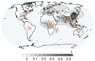
Figure 1 Anthropogenic aerosol optical depth of MACv2-SP for 2005. Locations of the nine aerosol plume centres are marked in orange with circles representing industrial pollution and rectangles representing seasonally active biomass burning.

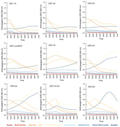
Figure 2 Future τ_i in the MACv2-SP interpretation of CMIP6 scenarios. Shown are the temporal developments of the anthropogenic aerosol optical depth, τ, at 550 nm in the colour-coded aerosol plumes of MACv2-SP for the nine emission scenarios of CMIP6.

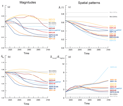
Figure 3 Future developments of global means in the MACv2-SP interpretation of CMIP6 scenarios. Shown are the temporal developments of annual averages in (a) $\stackrel{\mathrm{‾}}{\mathit{\tau }}$ at 550 nm for inducing aerosol–radiation interaction and (b) $\stackrel{\mathrm{‾}}{{\mathit{\eta }}_N}$ for mimicking aerosol–cloud interaction, as well as (c) hemispheric asymmetry in τ, $\stackrel{\mathrm{‾}}{A}$, weighted by the global mean $\stackrel{\mathrm{‾}}{\mathit{\tau }}$ and (d) the ratio of A at low latitudes (ϕ<36^∘) relative to higher latitudes. MACv2-SP's ranking of the emission scenarios of CMIP6 with respect to their strength in the forcing magnitude (a, b) and the spatial asymmetry (c, d) is shown using the colour-coded labels. Reference values of the mid-1970s and mid-2000s from the historical reconstruction (Fiedler et al., 2017; Stevens et al., 2017) are indicated by the grey lines.

2.2 Construction of aerosol scenarios in MACv2-SP

MACv2-SP has month-to-month and year-to-year changes in τ. We adopt the same annual cycle as used for the historical reconstruction (Stevens et al., 2017). The year-to-year changes in the future scenarios are derived from the gridded aerosol emissions of anthropogenic sources and open burning specified by the CMIP6 emission scenarios (Gidden et al., 2018). We construct time series of τ_i for each of the nine aerosol plume centres i using emission scaling factors, E_i(t) as function of year t of the Gregorian calendar:

$$\begin{array}{}\text{(1)}& {\mathit{\tau }}_i\left(t\right)={\mathit{\tau }}_i\left(\mathrm{2005}\right)E_i\left(t\right),\end{array}$$

where τ_i values in 2005 are the reference values from the MACv2 climatology (Sect. 2.1). The temporal scaling, E_i(t), for each of the nine aerosol scenarios in Table 2 are required input of the MACv2-SP parameterisation. They are available as MACv2-SP input files in netCDF format in the Supplement. The resulting anthropogenic aerosol τ_i(t) values for each scenario are presented in Sect. 3.1.

We construct E_i(t) from the gridded CMIP6 emissions, ϵ, of the chemical species, k:

$$\begin{array}{}\text{(2)}& E_i\left(t\right)={\displaystyle \frac{{\sum }_{k=\mathrm{1},\mathrm{2}}{w}_k\left[{\mathit{ϵ}}_{ik}\left(t\right)-{\mathit{ϵ}}_{ik}\left(\mathrm{1850}\right)\right]}{{\sum }_{k=\mathrm{1},\mathrm{2}}{w}_k\left[{\mathit{ϵ}}_{ik}\left(\mathrm{2005}\right)-{\mathit{ϵ}}_{ik}\left(\mathrm{1850}\right)\right]}}.\end{array}$$

The weight w_k describes the relative contribution of the two species, namely w₁=0.645 for SO₂ and w₂=0.355 for NH₃, motivated by the present-day ratio between sulphate and ammonia forcing as in Stevens et al. (2017). Following the approach by Stevens et al. (2017), we assume that the emission of all anthropogenic aerosol species scale with the emission of SO₂ and NH₃; therefore, we use these two species for scaling the anthropogenic aerosol optical depth of MACv2-SP over time. Furthermore, we use NH₃ emissions in addition to SO₂ to consider the fact that not all dominant aerosol emission changes over time scale with the SO₂ development. The approach is a simplification and is meant to facilitate experimentation and a better understanding of model errors (Stevens et al., 2017). Both emissions from open burning and otherwise classified anthropogenic sources are taken into account. Aerosol absorption is represented by the single scattering albedo (Sect. 2.1).

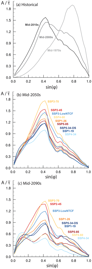
Figure 4 Hemispheric asymmetry of τ in the MACv2-SP interpretation of CMIP6 scenarios. Shown is the hemispheric asymmetry, A, weighted by the global mean τ. All values are computed for τ at 550 nm for (a) selected years from the historical reconstruction, as well as each CMIP6 emission scenario for both (b) the mid-2050s and (c) the mid-2090s.

Here, we use the gridded CMIP6 emission scenarios for the scaling, which is different from the emission scaling with ISO country codes in the historical reconstruction for MACv2-SP. For the scenarios, we average the anthropogenic emissions ϵ_ik in a $\mathrm{20}{}^{\circ }\times \mathrm{20}{}^{\circ }$ box around each plume centre, marked in Fig. 1, where τ_i(2005) is specified and scaled over time. The spatially averaged emission flux for these nine regions exceeds the global mean by a factor of 8.5, i.e. these regions capture the dominant anthropogenic sources and contribute a third of the total global anthropogenic emissions in 2005.

We test the reproducibility of the regional evolution of τ_i by scaling with emissions averaged around the plume centres. To do so, we derive E_i from a pre-existing aerosol emission database adopting the same spatial averaging, and compare the results to the corresponding E_i directly derived from the aerosol optical depth in a simulation with the aerosol–climate model ECHAM-HAM that uses the same aerosol emissions as boundary data (Fig. A1). Using spatial averages of aerosol emissions around the plume centres gives E_i similar to the direct scaling from the time-evolving aerosol optical depth from the complex model. Also, the results for E_i are not strongly sensitive to the choice of the number of grid boxes, e.g. a $\mathrm{10}{}^{\circ }\times \mathrm{10}{}^{\circ }$ box around the plume centres only weakly modifies E_i in most cases.

CMIP6 specifies emissions for 2015 and every 10th year from 2020 to 2100 (Gidden et al., 2018). We derive E_i(t) at the same times and apply a linear interpolation in between. The historical reconstruction ends in 2014 and the scenarios, beginning in 2015, have a slightly larger global mean of τ (by 0.0008) compared to 2014. Regional differences in the annual mean of τ are up to ±0.039 with smaller values for 2015 in East Asia, Europe, and North America, and larger values in the other plumes. The values of E_i(t) are all positive definite, except for the European plume in 2100 for SSP4-34 which has a weakly negative value of −0.01. This implies a slight reduction of the total aerosol burden relative to 1850 when anthropogenic aerosol was already present in Europe associated with the industrial revolution.

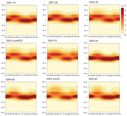
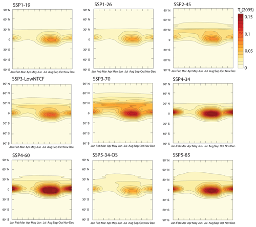
Figure 5 Spatial patterns for the mid-2090s in the MACv2-SP interpretation of CMIP6 scenarios. Shown are the annual cycles of the zonal means in τ at 550 nm weighted by the global mean $\stackrel{\mathrm{‾}}{\mathit{\tau }}$ for each month and emission scenario of CMIP6.

Table 1 Experiment set-up for estimating forcing.

The future changes in τ of the scenarios further scale MACv2-SP's magnitude of the induced Twomey effect. We mimic a Twomey effect by the prefactor, η_N, that is parameterised as function of latitude, ϕ, and longitude, λ:

$$\begin{array}{ll}{\displaystyle }{\mathit{\eta }}_N(\mathit{\varphi },\mathit{\lambda },t)& {\displaystyle }=\mathrm{1}+{\displaystyle \frac{\mathrm{d}N}{N}}\\ \text{(3)}& {\displaystyle }& {\displaystyle }={\displaystyle \frac{\ln \left[\mathrm{1000}\left[\mathit{\tau }(\mathit{\varphi },\mathit{\lambda },t)+{\mathit{\tau }}_{\mathrm{bg}}(\mathit{\varphi },\mathit{\lambda },t)\right]+\mathrm{1}\right]}{\ln \left[\mathrm{1000}{\mathit{\tau }}_{\mathrm{bg}}(\mathit{\varphi },\mathit{\lambda },t)+\mathrm{1}\right]}}.\end{array}$$

Multiplying η_N by the cloud droplet number concentration of the host model changes the cloud optical properties with the anthropogenic aerosol perturbation. The background aerosol optical depth, τ_bg, is an idealised plume-wise approximation consistent with the setting for the historical time period (Fiedler et al., 2017; Stevens et al., 2017):

$$\begin{array}{}\text{(4)}& {\mathit{\tau }}_{\mathrm{bg}}(\mathit{\varphi },\mathit{\lambda },t)={\mathit{\tau }}_{\mathrm{pl}}(\mathit{\varphi },\mathit{\lambda },t)+{\mathit{\tau }}_{\mathrm{gl}}.\end{array}$$

The components τ_pl refer to a plume-shaped background and τ_gl to a global constant. In the standard set-up of MACv2-SP, τ_gl is set to 0.02. This background is intended for MACv2-SP's aerosol–cloud interaction only and should not be confused with a natural aerosol pattern from observations. As emphasised by Stevens et al. (2017), this approach has been adopted so as to allow models to use their own natural aerosol for representing aerosol–radiation interaction, to optionally tune the radiation balance of models, and to keep a simple formulation of the Twomey effect for adjusting the magnitude. The Twomey effect (Twomey, 1974) is qualitatively understood, but the magnitude of aerosol–cloud interactions remains uncertain (Bellouin et al., 2019). Reasons for the difficulties in constraining the magnitude are, for instance, a shortage of suitable observations, model biases affecting radiative forcing, and the co-variability of meteorology and aerosol (e.g. Stevens and Feingold, 2009; Rosenfeld et al., 2014; Bony et al., 2015; Fiedler et al., 2016; Bellouin et al., 2019). As a result, different changes in N with aerosol have been proposed (Quaas et al., 2006; Andreae, 2009; Carslaw et al., 2013; Stevens et al., 2017). In the present work, we choose the original formulation by Stevens et al. (2017) for a consistent treatment from pre-industrial to the future projections. Note that stronger aerosol–cloud interactions are also plausible (Stevens, 2015; Bellouin et al., 2019) and can be represented by MACv2-SP, e.g. by reducing τ_gl in Eq. (4) as we do in a set of experiments here and elsewhere (Fiedler et al., 2017).

Table 2 Anthropogenic aerosol scenarios for MACv2-SP ($\stackrel{\mathrm{‾}}{\mathit{\tau }}=\mathrm{0.025}$ in 2015).

2.3 Calculation strategy for the aerosol forcing

We perform climate simulations for estimating the anthropogenic aerosol forcing. To do so, we use the atmosphere-only model configuration of MPI-ESM1.2 (Mauritsen et al., 2018) and follow the strategy by Fiedler et al. (2017). Natural variability internal to the model affects the effective radiative forcing estimates (Fiedler et al., 2017). To sufficiently account for the natural variability, we run ensembles of three simulations with the pre-industrial aerosol of 1850 and the anthropogenic aerosol from MACv2-SP. All simulations are performed for the period from 2000 to 2010 with the same annually repeating monthly anthropogenic aerosol patterns, e.g. monthly means of the year 2005. The simulations use the same year-to-year changes in the boundary conditions, e.g. observed sea-surface temperatures. The first year of each simulation is considered as the spin-up period and is not used in the data analyses.

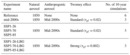
The set-ups of the experiments are summarised in Table 1. We choose three projections of τ in the mid-2090s to characterise the difference in the anthropogenic aerosol forcing, namely the SSP1-26, SSP3-70, and SSP5-85 scenarios that are introduced in Sect. 3.1. For these scenarios, we perform experiments with the standard settings for η_N that are consistent with the historical reconstruction of Stevens et al. (2017). Additionally, we perform experiments with increased η_N for each of these scenarios to quantify the sensitivity of the forcing differences to uncertainty in the magnitude of the Twomey effect. Here, we follow the method of the low background (LBG) experiments in Fiedler et al. (2017) and set τ_gl=0.002 which increases η_N (Eqs. 3 and 4) in the SSP1-26-LBG, SSP3-70-LBG, and SSP5-85-LBG experiments of the present article. The historical forcing estimate is for the mid-2000s aerosol pattern and is identical to the SP experiment in Fiedler et al. (2017).

We determine the instantaneous radiative forcing (RF) of anthropogenic aerosol for the scenarios in Table 1. RF is computed online by calling the radiative transfer calculation twice, i.e. once with and once without τ of MACv2-SP. As we have three simulations for each set-up with τ of MACv2-SP, we have 30 estimates of RF for each of the anthropogenic aerosol patterns. We further estimate the regional forcing efficiency as follows:

$$\begin{array}{}\text{(5)}& {\displaystyle \frac{\mathrm{RF}(\mathit{\varphi },\mathit{\lambda },t)}{\mathit{\tau }(\mathit{\varphi },\mathit{\lambda },t)}}\end{array}$$

for assessing the co-variability of RF with τ.

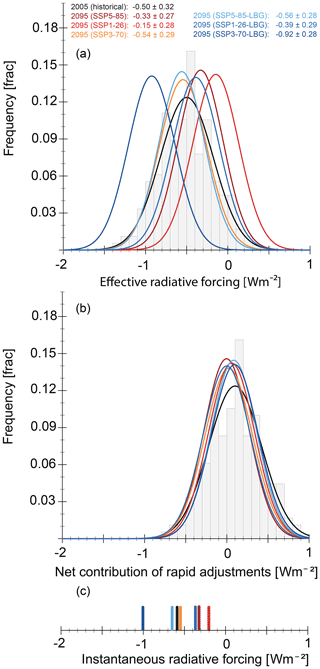
Figure 6 Natural variability in all-sky forcing for the mid-2090s. Shown are the Gaussian distributions of (a) the effective radiative forcing (ERF) and (b) the net contribution of rapid adjustments for the mid-2090s with the standard (orange–red) and the stronger (blue) Twomey effects. The black line marks the mid-2000s values from Fiedler et al. (2017) with the frequency histogram in grey. The distributions are based on annual means for all-sky condition in the shortwave spectrum (SW) at the top of the atmosphere (TOA). The long-term means ± year-to-year standard deviation of annual ERFs are listed at the top. The year-to-year standard deviation illustrates the impact of natural variability internal to the model for estimating ERF, in contrast to the (c) annual means in the instantaneous radiative forcing (RF) that are not strongly affected by natural variability.

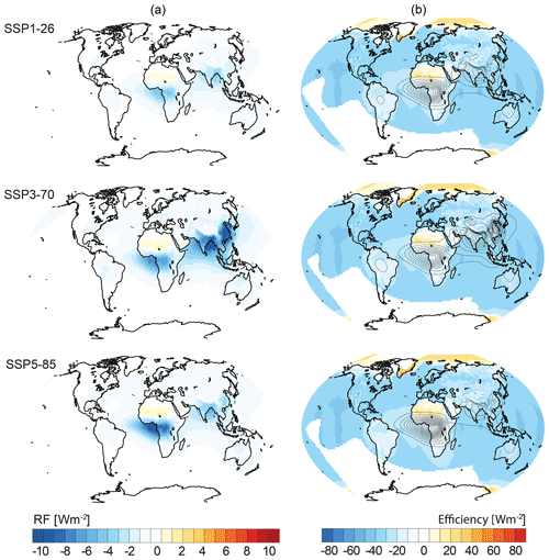
Figure 7 Clear-sky RF and efficiency for the mid-2090s. Shown are the (a) SW TOA instantaneous radiative forcing and (b) forcing efficiency as RF divided by τ. Contours show τ at 550 nm from 0.04 in steps of 0.04 (compare Fig. A3). All forcings are for clear-sky conditions in the mid-2090s from selected CMIP6 emission scenarios.

To calculate the effective radiative forcing (ERF) of anthropogenic aerosol relative to the pre-industrial period, we perform experiments without τ of MACv2-SP. For this reference set-up, we run an ensemble of six simulations for the period from 2000 to 2010 without anthropogenic aerosol, but with the same initial and boundary conditions as for the simulations with τ of MACv2-SP; this is undertaken to efficiently increase the number of estimates for ERF. ERF is determined as annual differences in the TOA shortwave radiation balance between the three simulations with τ from MACv2-SP and the six simulations without τ from MACv2-SP. As each simulation provides 10 years for the analysis, we yield a total of 180 annual estimates of ERF for each anthropogenic aerosol pattern. The net contribution of rapid adjustments is the difference between ERF and RF of anthropogenic aerosol.

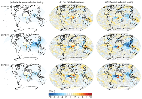
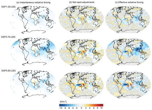
Figure 8 All-sky radiative forcing for the mid-2090s. Shown are the SW TOA (a) RF, (b) the net contribution from rapid adjustments, and (c) ERF for all-sky conditions in the mid-2090s from the CMIP6 emission scenarios. ERFs not significantly different from zero are masked out by hatching, adopting a confidence level of 10 %.

3 Results

3.1 Scenarios of future anthropogenic τ

3.1.1 Regionally averaged projections

The results for τ_i(t) are shown in Fig. 2 for each of the nine CMIP6 scenarios, listed in Table 2. Anthropogenic τ projections for East Asia are decreasing and reach levels comparable to the present-day conditions in Europe in the SSP1, SSP2, and SSP4 scenarios by the middle of the 21st century or later. The SSP3 and SSP5 scenarios also show decreasing τ by the end of the 21st century, but the level first increases and does not reduce as drastically as in the other SSPs. The development of Africa's anthropogenic τ is typically an increase by 2100. This projection is particularly pronounced in the SSP3 and SSP4 scenarios with an increase from 2015 to 2100 by factors of around 2–4. The SSP1 and SSP2 scenarios show slight τ_i increases in Africa only, whereas the SSP5 scenarios assume an increase in Africa's τ towards the 2040s and 2080s and a subsequent decrease. Anthropogenic τ in Europe and the Americas remain comparable to the low present-day levels.

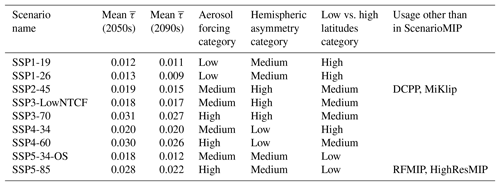
The analytical functions in MACv2-SP construct the temporally changing τ patterns from the time series of τ_i. Examples of the resulting spatial distributions of τ are shown for the mid-2050s and mid-2090s from all nine scenarios in the appendix (Figs. A2 and A3). In the following, we separate MACv2-SP's scenario interpretation into differences in global mean magnitudes and spatial patterns of τ. A summary of the global mean τ and the scenario categories is provided in Table 2.

Magnitude differences are shown as globally averaged $\stackrel{\mathrm{‾}}{\mathit{\tau }}$ and $\stackrel{\mathrm{‾}}{{\mathit{\eta }}_N}$ in Fig. 3. SSP3-70 stands out as the high-end scenario for both $\stackrel{\mathrm{‾}}{\mathit{\tau }}$ and $\stackrel{\mathrm{‾}}{{\mathit{\eta }}_N}$ with values exceeding the historical reconstruction for the mid-2000s and the mid-1970s. This scenario depicts socio-economic development failures associated with increasing air pollution (Riahi et al., 2017). Strong aerosol forcing is also expected from SSP4-60 and SSP5-85. In contrast, steep decreases in aerosol forcing are expected in SSP1, although τ reaches minima around 0.012 only after the 2030s. This scenario reflects the assumption of stringent pollution controls (Riahi et al., 2017). Towards the end of the 21st century, the difference in $\stackrel{\mathrm{‾}}{\mathit{\tau }}$ is largest between SSP3-70 and SSP1, with a range from 108 % to 36 % of the $\stackrel{\mathrm{‾}}{\mathit{\tau }}$ in 2015 (Table 2). Therefore, we build our estimates of the radiative forcing of anthropogenic aerosol for the mid-2090s on these scenarios (Sect. 3.2).

Figure 9 All-sky radiative forcing for the mid-2090s with strong Twomey effects. As Fig. 8, but with stronger Twomey effects due to increasing η_N (Sect. 2).

3.1.2 Spatial τ asymmetries

We assess the regional characteristics in the scenarios by quantifying hemispheric differences in τ, rather than comparing mean maps of τ. To do so, we first calculate the hemispheric asymmetry from zonally averaged $\stackrel{\mathrm{‾}}{\mathit{\tau }}$ for each latitude, ϕ:

$$\begin{array}{}\text{(6)}& A={\displaystyle \frac{\stackrel{\mathrm{‾}}{\mathit{\tau }\left(\mathit{\varphi }\right)}-\stackrel{\mathrm{‾}}{\mathit{\tau }(-\mathit{\varphi })}}{\mathrm{2}}}.\end{array}$$

In a second step, we divide A by the global mean of the same scenario, $\stackrel{\mathrm{‾}}{\mathit{\tau }}$, to screen out magnitude differences. The results are shown in Fig. 4. We find similarly large A for SSP2-45, SSP3-70, and SSP3-LowNTCF that are closest to the value for 2015. For all scenarios, A is particularly large in the tropics and subtropics, which is defined as regions equatorward of 36^∘ and referred to as low latitudes in the following.

All scenarios project a gradual decrease in the averaged hemispheric $\stackrel{\mathrm{‾}}{A}$ over the course of the 21st century. This implies that the zonally averaged τ becomes increasingly symmetrically distributed about the Equator in stark contrast to the historical reconstruction when most anthropogenic aerosol was in the Northern Hemisphere. We show these temporal evolutions of $\stackrel{\mathrm{‾}}{A}$ and also the ratio, ${\stackrel{\mathrm{‾}}{A}}_{\mathrm{low}\mathit{\varphi }}/{\stackrel{\mathrm{‾}}{A}}_{\mathrm{high}\mathit{\varphi }}$, of the mean $\stackrel{\mathrm{‾}}{A}$ at low latitudes relative to the high-latitude mean in Fig. 3. The mean ${\stackrel{\mathrm{‾}}{A}}_{\mathrm{low}\mathit{\varphi }}$ exceeds the value of ${\stackrel{\mathrm{‾}}{A}}_{\mathrm{high}\mathit{\varphi }}$ by at least a factor of 2 (Fig. 3), indicating that most τ is at latitudes equatorward of 36^∘, i.e. north of 36^∘ S and south of 36^∘ N. SSP4-34 has by far the strongest contrast between the low and high latitudes with a factor of roughly 11 in 2100, but the overall smallest hemispheric A. This behaviour reflects the relatively symmetric τ about the Equator (Fig. A3). The SSP1 scenarios also have stronger concentrations of anthropogenic aerosol at the low latitudes than further polewards, but a moderate hemispheric A compared to more extreme scenarios. Overall, the SSP5 scenarios have the smallest differences between the low and high latitudes.

The scenarios in MACv2-SP are constructed with the same scaling values for the annual cycles in τ, shown in Fig. 5. Their main differences in the annual cycle of τ are associated with the variety in the spatial patterns. Similarities amongst the scenarios are marked (1) tropical τ maxima in the SSP4 and SSP5-85 scenarios for the period from June to January, and (2) northern high-latitude τ maxima in SSP2, SSP3, and SSP5. The former maxima are associated with anthropogenic aerosol from biomass burning, whereas the latter is dominated by industrial emissions.

Table 3 Mid-2090s anthropogenic aerosol SW (E)RF at TOA from MACv2-SP as long-term averages ± year-to-year standard deviation in W m⁻².

3.2 Radiative forcing of anthropogenic aerosol

3.2.1 Global means

We choose three scenarios for assessing the differences in the radiative forcing of anthropogenic aerosol in the mid-2090s associated with the choice of the emission pathway (Table 1). These are SSP3-70 as a high-end scenario and SSP1-26 as a lower bound for the differences in $\stackrel{\mathrm{‾}}{\mathit{\tau }}$ of 0.009 to 0.027 at the end of the 21st century. The third scenario choice is SSP5-85 which also has a high $\stackrel{\mathrm{‾}}{\mathit{\tau }}$ of 0.022, but interesting differences in the spatial patterns compared to SSP3-70. SSP5-85 projects most aerosol in Africa, while SSP3-70 projects most aerosol in Asia. The aerosol in Africa is seasonally dominated by biomass burning (Sect. 2.1), whereas the aerosol in East Asia is primarily associated with industrial emissions (Sect. 2.1). Therefore, SSP3-70 has the largest hemispheric $\stackrel{\mathrm{‾}}{A}$ (Fig. 4), whereas the annual cycle in SSP5-85 is more strongly pronounced due to the seasonally active biomass burning in Africa (Figs. 5 and A4).

Table 3 summarises the global mean estimates of RF and ERF. Compared to the mid-2000s, RF and ERF decrease in all scenarios, except in SSP3-70 which has the highest aerosol burden. In SSP3-70, the mid-2090s ERF of −0.54 W m⁻² is slightly stronger than the historical estimate of −0.50 W m⁻² for the mid-2000s from Fiedler et al. (2017). The mid-2090s RF and ERFs are 33 %–95 % and 30 %–108 % of the mid-2000s estimates, respectively. The forcing of −0.15 to −0.54 W m⁻² for the mid-2090s describes the difference associated with the future emission pathways alone. When we assume a stronger magnitude of the Twomey effect, we get more negative ERFs of −0.39 to −0.92 W m⁻² (Table 3). Our forcing values are consistent with earlier studies, namely the scenario difference of −0.7 to −1.0 W m⁻² at the end of the 21st century from the CMIP5 configuration of HadGEM2-ES (Bellouin et al., 2011), the ACCMIP model mean estimate of −0.12 W m⁻² for 2100 (Shindell et al., 2013), and the scenario difference in clear-sky RF of −0.24 to −0.37 W m⁻² for 2100 from Lamarque et al. (2011).

Estimating ERF requires accounting for variability internal to the model. Figure 6 shows the distribution of yearly estimates of ERF from the ensemble of simulations for the mid-2090s. It can be noted that the year-to-year standard deviations of around 0.3 W m⁻² are comparable between the mid-2000s and all of our projections for the mid-2090s. This behaviour reflects that a precise estimate of ERF for any given aerosol distribution and strength requires averaging over several decades (Fiedler et al., 2017). Particularly when the ERF is small, e.g. for SSP1-26, the year-to-year standard deviation is even larger than the ERF itself (Table 3). Compared to the ERF, the year-to-year standard deviation of the RF is small, indicative of comparably stable estimates such that a 1-year mean is typically sufficient for a precise estimate of a model's RF. This implies that the model-internal variability in ERF is primarily associated with the variability in the net contribution of rapid adjustments (Fig. 6).

3.2.2 Spatial patterns

The regional pattern of the clear-sky contributions to RF resembles the distribution of τ, shown in Fig. 7. Here, negative radiative effects correlate with increasing τ, as shown by the similarity of the patterns in forcing efficiency for all three scenarios of different forcing strengths. Most regions show the expected negative radiative effects associated with anthropogenic aerosol. The only exception is northern Africa, where the more strongly absorbing aerosol at the edge of the biomass burning plume induces weakly positive radiative effects over the strongly reflective desert surface. In all-sky conditions, the patterns are to a great extent similar to those in clear-sky, but clouds mask parts of the negative radiative effects such that the regional all-sky contributions to RF are typically less negative (Fig. 8).

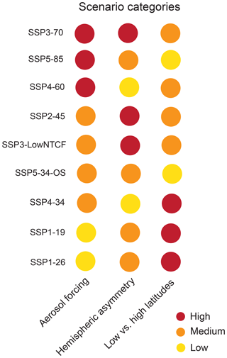
Figure 10 Categories in the MACv2-SP interpretation of the CMIP6 anthropogenic aerosol scenarios. Shown is the colour-coded ranking of the CMIP6 scenarios with respect to the strength of the aerosol forcing, the hemispheric asymmetry, and the low- to high-latitude difference in the asymmetry.

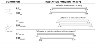
Figure 11 Difference in anthropogenic aerosol radiative forcing of the MACv2-SP interpretation of the CMIP6 scenarios for the mid-2090s. Summarised are the instantaneous (RF) and effective radiative forcing (ERF) from aerosol–radiation interaction (ARI) and aerosol–cloud interaction (ACI), based on the high-end SSP3-70 and SSP5-85 scenarios, and SSP1-26 as a low-emission scenario for the upper bound. The bars illustrate the difference in forcing associated with the emission pathways of CMIP6.

Including rapid adjustments strongly impairs the detectability of significant radiative effects for the mid-2090s aerosol patterns. Figures 8 and 9 show the similarly strong impact of atmospheric variability on the ERF for both high (SSP3-70) and low (SSP1-26) aerosol forcing categories as well as different strengths of the Twomey effect. The impact of natural variability is consistent with findings for the patterns of the mid-1970s and mid-2000s (Fiedler et al., 2017). An interesting feature in the projection for the mid-2090s is the positive forcing in parts of central Africa. This pattern emerges primarily from rapid adjustments in the atmosphere with a relative smaller regional contribution from RF (Fig. 8). In our model, the radiative forcing of anthropogenic aerosol from aerosol–radiation interaction and the Twomey effect induce heating perturbations. The associated change in the air temperature affects, for instance, the static stability of the atmosphere and thereby the circulation and embedded clouds. Such rapid adjustments cause the difference between ERF and RF, and are summarised here as net contribution.

4 Conclusions

The present article presents the MACv2-SP interpretation of the future CMIP6 emissions of anthropogenic aerosol. We show the construction of the scaling parameter for the aerosol optical depth, τ, for 2015–2100 and the resulting spatio-temporal distribution of τ. The highlights of the projected aerosol developments for the 21st century are (1) a continuous stabilisation or further decrease in τ in Europe and the Americas, (2) a long-time decrease of τ in East Asia stretching over the next decades in many scenarios, and (3) steep increases in τ in Africa's biomass burning regions in most scenarios. We rank the scenarios with respect to their strengths in the aerosol forcing magnitude, the hemispheric asymmetry, and the low- to high-latitude asymmetry, summarised in Fig. 10.

We estimate the differences in the radiative forcing of anthropogenic aerosol at the end of the 21st century that are associated with the choice of the future aerosol emission scenario (Fig. 11). To do so, we choose three aerosol forcing scenarios that include the high- and low-end scenarios of τ in the mid-2090s (SSP5-85, SSP3-70, and SSP1-26). Their MACv2-SP aerosol is prescribed in ensembles of simulations with the atmosphere-only configuration of MPI-ESM1.2 (Mauritsen et al., 2018), participating in CMIP6 and endorsed MIPs. The ensemble is useful for estimating the effective radiative forcing in light of natural variability internal to models (Fiedler et al., 2017). The year-to-year standard deviation in ERF of roughly 0.3 W m⁻² illustrates the impact of natural variability on ERF estimates that almost exclusively stems from the variability in the net contribution from rapid adjustments. Averaging over sufficiently long time periods, here 180 years, accounts for that variability. MPI-ESM1.2 gives −0.15 W m⁻² with SSP1-26 to −0.54 W m⁻² with SSP3-70 for the ERF of anthropogenic aerosol for the mid-2090s (Fig. 11), reflecting the overall differences due to the anthropogenic emission pathways alone. The clear-sky forcing of SSP1-26 and SSP3-70 is slightly stronger with values of −0.24 and −0.69 W m⁻², respectively, as the clouds mask the radiative effects of anthropogenic aerosol. Assuming a stronger Twomey effect gives more negative all-sky ERFs of −0.39 to −0.92 W m⁻² for the mid-2090s.

MACv2-SP's interpretation of the CMIP6 emission scenarios will be applied in MIPs endorsed by CMIP6 and other research activities ranging from high-resolution modelling via seasonal and decadal climate predictions to climate-change studies. The strength of the anthropogenic aerosol forcing has implications for the temperature development in simulations with coupled atmosphere–ocean models, e.g. a relatively weak aerosol forcing as utilised in the standard setting of MACv2-SP likely results in a relatively stronger warming signal. Past studies have highlighted the role of aerosol radiative forcing for climate changes (e.g. Chung and Soden, 2017), underlining the importance of better understanding the uncertainty of anthropogenic aerosol forcing. Research initiatives such as the Radiative Forcing Model Intercomparison Project (RFMIP, Pincus et al., 2016) can help to make progress in understanding model biases causing diversity in aerosol forcing. RFMIP adopts MACv2-SP including the high-end SSP5-85 scenario presented here and will provide aerosol forcing estimates from 1850 to 2100. All scenario input files for MACv2-SP are freely available in the Supplement of this publication. We hope MACv2-SP's scenarios will be useful for advancing our understanding of climate change and supporting impact studies for informing stakeholders.

Appendix A

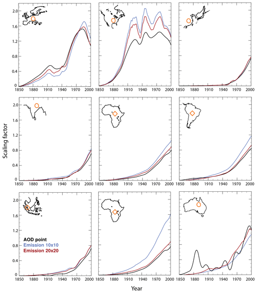
Figure A1 Scaling factor comparison. Shown are annual scaling factors E_i(t) derived from (black) the aerosol optical depth in the plume centres of a transient ECHAM-HAM simulation using a pre-existing aerosol emission database, and (colours) the anthropogenic aerosol emissions of that simulation, averaged over grid boxes around the plume centres. The geographical positions of the plumes with industrial pollution (circles) and biomass burning (rectangles) are indicated.

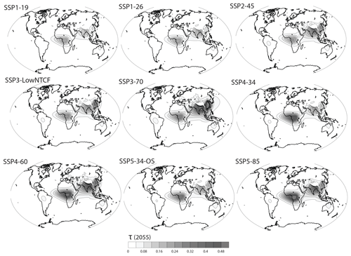
Figure A2 τ scenarios for the mid-2050s in MACv2-SP. Shown are the spatial distributions of τ at 550 nm in the mid-2050s for each of the nine emission scenarios of CMIP6.

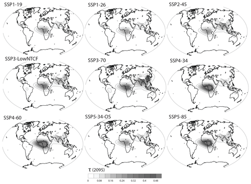
Figure A3 τ scenarios for the mid-2090s in MACv2-SP. As in Fig. A2, but projection for the mid-2090s.

Figure A4 τ scenarios for the mid-2090s in MACv2-SP. Shown are the annual cycles of the zonal means in τ at 550 nm in the mid-2090s for each of the nine emission scenarios of CMIP6.