BGC-val: a model- and grid-independent Python toolkit to evaluate marine biogeochemical models

The biogeochemical evaluation toolkit, BGC-val, is a model- and grid-independent Python toolkit that has been built to evaluate marine biogeochemical models using a simple interface. Here, we present the ideas that motivated the development of the BGC-val software framework, introduce the code structure, and show some applications of the toolkit using model results from the Fifth Climate Model Intercomparison Project (CMIP5). A brief outline of how to access and install the repository is presented in Appendix A, but the specific details on how to use the toolkit are kept in the code repository.

The key ideas that directed the toolkit design were model and grid independence, front-loading analysis functions and regional masking, interruptibility, and ease of use. We present each of these goals, why they were important, and what we did to address them. We also present an outline of the code structure of the toolkit illustrated with example plots produced by the toolkit.

After describing BGC-val, we use the toolkit to investigate the performance of the marine physical and biogeochemical quantities of the CMIP5 models and highlight some predictions about the future state of the marine ecosystem under a business-as-usual CO₂ concentration scenario (RCP8.5).

1 Introduction

It is widely known that climate change is expected to have a significant impact on weather patterns, the cryosphere, the land surface, and the ocean (Cook et al., 2013; Le Quéré et al., 2013; Rhein et al., 2013; Stocker et al., 2015). Marine organisms are vulnerable not only to impacts of rising temperatures, but also to the associated deoxygenation (Gruber, 2011; Stramma et al., 2008) and ocean acidification driven by ocean CO₂ uptake (Azevedo et al., 2015; Caldeira and Wickett, 2003; Dutkiewicz et al., 2015). The ocean is an important sink of carbon, absorbing approximately 27 % of the anthropogenic carbon emitted between 2002 and 2011 (Le Quéré et al., 2013). Under a changing climate, the ocean is likely to continue to absorb some of the anthropogenic atmospheric carbon dioxide, rendering the ocean more acidic via the increased formation of carbonic acid. The acidification of the ocean is expected to continue to have a significant impact on sea life (Dutkiewicz et al., 2015; Rhein et al., 2013). Due to the high thermal capacity of water, nearly all of the excess heat captured by the greenhouse effect is absorbed by the ocean (Rhein et al., 2013). This increases the temperature of the waters, which causes sea levels to rise via thermal expansion (Church et al., 2013), may accelerate the melting of sea ice (Moore et al., 2015), and may push many marine organisms outside of their thermal tolerance range (Poloczanska et al., 2016).

The 2016 Paris Climate Accord is a wide-ranging international agreement on greenhouse gas emissions mitigation and climate change adaptation which is underpinned by the goal of limiting the global mean temperature increase to less than 2 ^∘C above pre-industrial levels (Schleussner et al., 2016). International environmental policies like the Paris Climate Accord hinge on the projections made by the scientific community. Numerical models of the Earth system are the only tools available to make meaningful predictions about the future of our climate. However, in order to trust the results of the models, they must first be demonstrated to be a sufficiently good representation of the Earth system. The process of testing the behaviour of the simulations is known as model evaluation. The importance of evaluating the models grows in significance as models are increasingly used to inform policy (Brown and Caldeira, 2017).

The Coupled Model Intercomparison Project (CMIP) is a framework for coordinating climate change experiments and providing information of value to the International Panel on Climate Change (IPCC) Working Groups (Taylor et al., 2012). CMIP5 was set up to address outstanding scientific questions, to improve understanding of climate, and to provide estimates of future climate change that will be useful to those considering its possible consequences (Meehl et al., 2009; Taylor et al., 2007). These models represent the best scientific projections of the range of possible climates going into the 21st century. The results of previous rounds of CMIP comparisons have become a crucial component of the IPCC reports. In the fifth phase of CMIP, many of the climate forecasts were based on representative concentration pathways (RCPs), which represented different possibilities for greenhouse gas concentrations in the 21st century (Moss et al., 2010; van Vuuren et al., 2011).

The upcoming Sixth Climate Model Intercomparison Project, CMIP6 (Eyring et al., 2016), is expected to start receiving models in the year 2018. In order to contribute to CMIP6, each model must complete a suite of scenarios known as the Diagnosis, Evaluation, and Characterisation of Klima (DECK) simulations, which include an atmospheric model intercomparison between the years 1979 and 2014, a pre-industrial control simulation, a 1 % per year CO₂ increase, an abrupt 4×CO₂ run, and a historical simulation using CMIP6 forcings (1850–2014). CMIP6 models are also required to use consistent standardisation, coordination, infrastructure, and documentation.

Numerical simulations are the only tools available to predict how rising temperature, atmospheric CO₂, and other factors will influence marine life in the future. Furthermore, Earth system models are also the tool that can project how changes in the marine system feed back on and interact with other climate-relevant components of the Earth system. The UK Earth system model (UKESM1) is a next-generation Earth system model currently under development. The aim of UKESM1 is to develop and apply a world-leading Earth system model. Simulations made with the UKESM1 will be contributed to CMIP6.

During the process of building the UKESM1, we also deployed a suite of tools to monitor the marine component of the model as it was being developed. This software suite is called BGC-val, and it is used to compare the marine components of simulations against each other and against observational data, with an emphasis on marine biogeochemistry. The suite of evaluation tools that we present in this work is a generalised extension of those tools. BGC-val has been deployed operationally since June 2016 and has been used extensively for the development, evaluation, and tuning of the spin-up and CMIP6 DECK runs of the marine component of the UKESM1, MEDUSA (Yool et al., 2013). The earliest version of BGC-val was based on the tools used to evaluate the development of the NEMO-ERSEM simulations in the iMarNet project (Kwiatkowski et al., 2014).

The focus of this work is not to prepare a guide on how to run the BGC-val code, but rather to present the central ideas and methods used to design the toolkit. A brief description of how to install, set up, and run the code can be found in the Appendix A. Further details are available in the README.md file, which can be found in the base directory of the code repository. Alternatively, the README.md file can be viewed by registered users on the landing page of the BGC-val toolkit GitLab server. Instructions on how to register and access the toolkit can be found below in the “Code availability” section. After this introduction, Sect. 2 outlines the features of the BGC-val toolkit, Sect. 3 describes the evaluation process used by the toolkit, and Sect. 4 describes the code structure of the BGC-val toolkit. Finally, Sect. 5 shows some examples of the toolkit in use with model data from CMIP5.

Model evaluation tools

The evaluation of marine ecosystem models is a crucial stage in the deployment of climate models to inform policy decisions. When compared to models of other parts of the Earth system, marine models have several unique features which complicate the model evaluation process. The data available for evaluating a marine model can be relatively scarce. The ocean covers more than twice as much of the surface of the Earth than land, and there are sizeable regions of the ocean which are rarely visited by humans, let alone sampled by scientific cruises (Garcia-Castellanos and Lombardo, 2007). In addition, only the surface of the ocean is visible to satellites; the properties of marine life in the deep waters cannot be observed from remote sensing. Similarly, the connections between different components of the Earth system can also be difficult to measure. Several crucial global fluxes are unknown or estimated with significant uncertainties, such as the global total flux of CO₂ into the ocean (Takahashi et al., 2009), the global total deposition of atmospheric dust (Mahowald et al., 2005), or the global production export flux (Boyd and Trull, 2007; Henson et al., 2011). Prior to the development of BGC-val, there was no evaluation toolkit specific to models of the marine ecosystem and evaluation was typically performed in an ad hoc manner.

As part of the preparation for CMIP6, a community diagnostic toolkit for evaluating climate models, ESMValTool, has been developed (Poloczanska et al., 2016). Like BGC-val, ESMValTool is a flexible Python-based model evaluation toolkit and many of the features developed for BGC-val also appear in ESMValTool. However, BGC-val was developed explicitly for evaluating models of the ocean, whereas ESMValTool was built to evaluate models of the entire Earth system. It must be noted that ESMValTool was not yet available for operational deployment when we started evaluating the UKESM1 spin in June 2016. Furthermore, ESMValTool contained very few ocean and marine biogeochemistry performance metrics at that point. The authors of ESMValTool are currently in the process of preparing ESMValTool version 2 for release in the autumn of 2018. This is a rapidly developing package, with several authors adding new features every week, and it is not likely to be finalised for operational deployment for several more months. However, many of the features that were implemented in BGC-val have since also been added to ESMValTool and the authors of BGC-val are also contributors to ESMValTool. In addition, many of the metrics deployed in BGC-val's ocean-specific evaluation have been proposed as key metrics to include in future versions of ESMValTool. A full description and access to the ESMValTool code is available via the GitHub page: https://github.com/ESMValGroup/ESMValTool (last access: 5 October 2018).

Marine Assess (formerly Ocean Assess) is a UK Met Office software toolkit for evaluating the physical circulation of the models developed there. From the authors' hands-on experience with Marine Assess, several of its metrics were specific to the NEMO ORCA1 grid, so it could not be deployed to evaluate the other CMIP5 models. Furthermore, Marine Assess is not available outside the UK Met Office and is not yet described in any public documentation. For these reasons, while Marine Assess is a powerful tool, it has yet to be embraced by the wider model evaluation community (Daley Calvert and Tim Graham, Marine Assess authors, Met Office UK, personal communication, 2018).

Outside of the marine environment, several toolkits are also available for evaluating models of the other parts of the Earth system. For the land surface, the Land surface Verification Toolkit (LVT) and the International Land Model Benchmarking (ILAMB) frameworks are available (Hoffman et al., 2017; Kumar et al., 2012). For the atmosphere, several packages are available, for instance the Atmospheric Model Evaluation Tool (AMET) (Appel et al., 2011), the Chemistry–Climate Model Validation Diagnostic (CCMVal-Diag) tool (Gettelman et al., 2012), or the Model Evaluation Tools (MET) (Fowler et al., 2018). Please note that these are not complete lists of the tools available.

Also note that in this work, we do not aim to introduce any new metrics or statistical methods. There are already plenty of valuable metrics and method descriptions available (Jolliff et al., 2009; Saux Picart et al., 2012; Stow et al., 2009; Taylor, 2001; de Mora et al., 2013, 2016).

In addition to the statistical tools available, the marine biogeochemistry community has access to many observational datasets. BGC-val has been used to compare various ocean models against a wide range of marine datasets, including the Takahashi air–sea flux of CO₂ (Takahashi et al., 2009), the European Space Agency Climate Change Initiative (ESA-CCI) ocean colour dataset (Grant et al., 2017), the World Ocean Atlas data for temperature (Locarnini et al., 2013), salinity (Zweng et al., 2013), oxygen (Garcia et al., 2013a), and nutrients (Garcia et al., 2013b), and the MAREDAT (Buitenhuis et al., 2013b) global database for marine pigment (Peloquin et al., 2013), picophytoplankton (Buitenhuis et al., 2012), diatoms (Leblanc et al., 2012), and mesozooplankton (Moriarty and O'Brien, 2013). These datasets are all publicly available and are typically distributed as a monthly climatology or annual mean NetCDF file.

2 The BGC-val toolkit design features

While BGC-val was originally built as a toolkit for investigating the time development of the marine biogeochemistry component of the UK Earth system model, UKESM1, the primary focus of BGC-val's development was to make the toolkits as generic as possible. This means that the tools can be easily adapted for use with for a wide range of models, spatial domains, model grids, fields, datasets, and timescales without needing significant changes to the underlying software and without any significant post-processing of the model or observational data. The toolkit was built to be model independent, grid independent, interruptible, simple to use, and to include front-loading analyses and masking functionality.

The BGC-val toolkit was written in Python 2.7. The reason that Python was used is because it is freely available and widely distributed; it is portable and available with most operating systems, and there are many powerful standard packages that can be easily imported or installed locally. It is object oriented (allowing front-loading functionality described below), and it is popular and hence well documented and well supported.

2.1 Model independence

The Earth system models submitted to CMIP5 were created by largely independent groups of scientists. While some model developers build CMIP compliance into their models, other model developers choose to use their in-house style, then reformat the file names and contents to a uniform naming and units scheme before they are submitted to CMIP. This flexibility means that each model working group may use their own file-naming conventions, dimension names, variables, and variable names until the data are submitted to CMIP5. Outside of the CMIP5 standardisation, there are many competing nomenclatures. For instance, in addition to the CMIP standard name, lat, we have encountered the following nonstandard names in model data files, all describing the latitude coordinate: lats, rlat, nav_lat, latitude, and several other variants. Similarly, different models and observational datasets may not necessarily use the same units.

While the CMIP5 data have been produced using a uniform naming scheme, this toolkit allows for models to be evaluated without any prior assumptions on their naming conventions or units. This means that it would be possible to deploy this toolkit during the development stage of a model, before reformatting the data to CMIP compliance. This is how this toolkit was applied during the development of UKESM1. Model independency ensures that the toolkit can be applied in a range of scenarios, without requiring significant knowledge of the toolkit's inner workings and without post-processing the data.

2.2 Grid independence

For each Earth system model submitted to CMIP5, the development team chose how they wanted to divide the ocean into a grid composed of individual cells. Furthermore, unlike the naming and unit schemes, the model data submitted to CMIP5 have not been reformatted to a uniform grid.

The BGC-val toolkit was originally built to work with NEMO's extended eORCA1 grid, which is a tri-polar grid with an irregular distribution of two-dimensional latitude and longitude coordinates. However, information about the grid is supplied alongside the model data such that there is no grid requirement hard-wired into BGC-val. This means that the toolkit is capable of handling any kind of model grid, whether it be a regular grid, reversed grid, a tri-polar grid, or any other type of grid, without the need to re-interpolate the data to a common grid.

When calculating means, medians, and other metrics, the toolkit uses the grid cell area or volume to weight the results. This means that it is possible to use this toolkit to compare multiple models that use different grids without the computationally expensive and potentially lossy process of re-interpolation to a common grid. The CMIP5 datasets include grid cell area and volume. However, outside the CMIP standardised datasets, most models and observational datasets provide grid cell boundaries or corner coordinates as well as longitude and latitude cell-centred coordinates. These corners and boundaries can be used to calculate the area and volume of each grid cell. If only the cell-centred points are provided, the BGC-val toolkit is able to estimate the grid cell area and volume based on the coordinates.

2.3 Front-loaded analysis functionality

While extracting the data from file, BGC-val can apply an arbitrary predefined or user-defined mathematical Python function to the data. This means that it is straightforward to define a customised analysis function in a Python script, then to pass that function to the evaluation code, which then applies the analysis function to the dataset as the data are loaded. Firstly, this method ensures that the toolkit is not limited to a small set of predefined functions. Secondly, the end users are not required to go deep into the code repository in order to use a customised analysis function.

In its simplest form, the front-loading functionality allows a straightforward conversion of the data as they are loaded. As a basic example, it would be straightforward to add a function to convert the temperature field units from Celsius to Kelvin. The Celsius to Kelvin function would be written in a short Python script, and the script would be listed by name in the evaluation's configuration file. This custom function would be applied while loading the data, without requiring the model data to be pre-processed or for the BGC-val inner workings to be edited in depth.

Similarly, more complex analysis functions can also be front loaded in the same way. For instance, the calculation of the global total volume of oxygen minimum zones, the total flux of CO₂ from the atmosphere to the ocean, and the total current passing though the Drake Passage are all relatively complex calculations which can be applied to datasets. These functions are also already included in the toolkit in the functions folder described in Sect. 4.3.1.

2.4 Regional masking

Similarly to the front-loading analyses described above in Sect. 2.3, BGC-val users can predefine a customised region of interest, then ignore data from outside that region. The regional definitions are supplied in advance and can be used to evaluate several models or datasets. The process of hiding data from regions that are not under investigation is known as “masking”. In addition, while the UKESM and other CMIP models are global models, there is no requirement for the model to be global in scale; regional and local models can also be investigated using BGC-val.

While BGC-val already includes many regional masks, it is straightforward to define new masks that hide regions which are not under investigation. Similarly to Sect. 2.3, the new masks can be defined in advance, named, and called by name, without having to go deep into the toolkit code. These masks can be defined in terms of the latitude, longitude, depth, time range, or even the data. The toolkit includes several standard masks; for example, there is a mask which allows the user to retrieve only data in the Northern Hemisphere, called NorthernHemisphere, or to ignore all data deeper than 10 m, called Depth_0_10m.

However, more complex masks could be created. For instance, it is feasible to make a custom mask which ignores data below the 5th percentile or above the 95th percentile. It is also possible to stack masks by applying two or more masks successively in a custom mask.

For instance, a hypothetical custom mask could mask data below a depth of 100 m, ignoring the Southern Ocean and also remove all negative values. This means that it is straightforward for users to add arbitrarily complex regional masks to the dataset. For more details, please see Sect. 4.3.2.

2.5 Interruptible

BGC-val makes regular save points during data processing such that the analysis can be interrupted and restarted without reprocessing all the data files from the beginning. This means that each analysis only needs to run once. Alternatively, it means that it is possible to evaluate on-going model simulations, without reprocessing everything every time that the evaluation is needed.

The processed data are saved as Python shelve files. Shelve files allow for any Python object, including data arrays and dictionaries, to be committed to disc. As the name suggests, shelving allows for Python objects to be stored and reloaded at a later stage. These shelve files help with the comparison of multiple models or regions, as the evaluation results can be set aside, then quickly reloaded later to be processed into a summary figure, or pushed into a human-readable data file.

2.6 Ease of use

A key goal was to make the toolkit straightforward to access, install, set up, and use. The code is accessed using a GitLab server, which is a private online graphical user interface to the version control software, Git, similar to the commercial GitHub service. This makes it straightforward for multiple users to download the code, report bugs, develop new features, and share the changes. Instructions on how to register and access the toolkit can be found below in the “Code availability” section. Once it has been cloned to your local workspace, BGC-val behaves like a standard Python package and can be installed via the “pip” interface.

More importantly, BGC-val was built such that entire evaluation suites can be run from a single human-readable configuration file. This configuration file uses the .ini configuration format and does not require any knowledge of Python or the inner workings of BGC-val. The configuration file contains all the paths to data, descriptions of the data file and model data, links to the evaluation function, Boolean switches to turn on and off various evaluation metrics, the names of the variables needed to perform an evaluation, and the paths for the output files. This makes it possible to run the entire package without having to change more than a single file. The configuration file is described in Sect. 4.1. BGC-val also summarises the results into an html document, which can be opened directly in a web browser, and evaluation figures can be extracted for publication or sharing. The summary report is described in Sect. 4.2.3. An example of the summary report is included in the Supplement.

3 Evaluation process

In this section, we describe the five-stage evaluation process that the toolkit applies to model and observational data. Figure 1 summarises the evaluation process graphically.

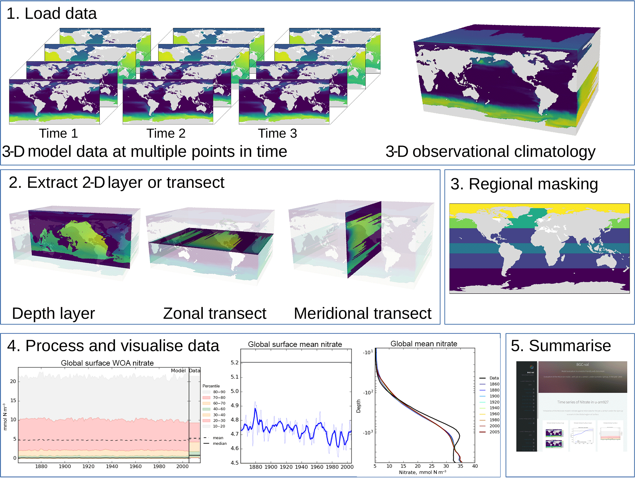
Figure 1 The five stages of the evaluation process. The first stage is the loading of the model and observational data. The second stage is the extraction of a two-dimensional array. The third stage is regional masking. The fourth stage is processing and visualisation of the data. The fifth stage is the publication of an html summary report. Note that the three figures shown in the fourth stage are repeated below in Figs. 3, 4, and 6.

3.1 Load model and observational data

The first stage of the evaluation process is to load the model and observational data. The model data are typically a time series of two- or three-dimensional variables stored in one or several NetCDF files. Please note that we use the standard convention of only counting spatial dimensions. As such, any mention of dimensionality here implies an additional temporal dimension; i.e. three-dimensional model data have length, height, width, and time dimensions.

The model data can be a single NetCDF variable or some combination of several variables. For instance, in some marine biogeochemistry models, total chlorophyll concentration is calculated as the sum of many individual phytoplankton functional type chlorophyll concentrations. In all cases, BGC-val loads the model data one time step at the time, whether the NetCDFs contain one or multiple time steps.

The front-loading evaluation functions described in Sects. 2.3 and 4.3.1 are applied to each time step of the model data at this point. The resulting loaded data can be a one-, two-, or three-dimensional array. The use of an observational dataset is optional, but allows the model to be compared against historical measurements. The observational data and model data are not required to be loaded using the same function.

When loading data, BGC-val assumes that we use the NetCDF format. The NetCDF files are opened in BGC-val with a custom Python interface, dataset.py, in the bgcvaltools package. The dataset class is based on the standard Python netCDF4.Dataset class. NetCDF files are composed of two parts, the header and the data. The header typically includes all the information needed to understand the origin of the file, while the data contain a series of named variables. Each named variable should (but not obligatorily) include their dimensions, units, their long name, their data, and their mask. Furthermore, the dimensions in NetCDF format are not restricted to regular latitude–longitude grids. Some NetCDFs use arbitrary dimensions, such as a grid cell index, irregular grids like NEMO's eORCA1 grid, or even triangular grid cells as in the Finite Volume Coastal Ocean Model (FVCOM) (Chen et al., 2006).

3.2 Extract a two-dimensional slice

The second evaluation stage is the extraction of a two-dimensional variable from three-dimensional data. As shown in the second panel of Fig. 1, the two-dimensional variable can be the surface of the ocean, a depth layer parallel to the surface, an east–west transect parallel to the Equator, or a north–south transect perpendicular to the Equator. This stage is included in order to speed up the process of evaluating a model; in general, it is much quicker to evaluate a 2-D field than a 3-D field. Furthermore, the spatial and transect maps produced by the evaluation process can become visually confusing when overlaying several layers. Note that stages 2 and 3 are applied to both model and observational data (if present). This stage is unnecessary if the data loaded in the first stage are already a two-dimensional variable, such as the fractional sea ice coverage, or a one-dimensional variable, such as the Drake Passage Current.

In the case of a transect, instead of extracting along the file's internal grid, the transect is produced according to the geographic coordinates of the grid. This is done by locating points along the transect line inside the grid cells based on the grid cell corners.

3.3 Extract a specific region

Stage 3 is the masking of specific regions or depth levels from the 2-D extracted layer, as described in Sect. 2.4. Stage 3 is not needed if the variable is already a one-dimensional product, such as the total global flux of CO₂. Stage 3 takes the two-dimensional slice, then converts the data into five one-dimensional arrays of equal length. These arrays represent the time, depth, latitude, longitude, and value of each data point in the data. These five 1-D arrays can be further reduced by making cuts based on any of the coordinates or even cutting according to the data.

Both stages 2 and 3 of the evaluation process reduce the number of grid cells under evaluation. This two-stage process is needed because the stage 3 masking cut can become memory intensive. As such, it is best to for the data to arrive at this stage in a reduced format. In contrast, the stage 2 process of producing a 2-D slice is a relatively computationally cheap process. This means that the overall evaluation of a model run can be done much faster.

3.4 Produce visualisations

Stage 4 is the processing of the two-dimensional datasets and the creation of visualisations of the model and observational data. Figure 1 shows three examples of the visualisations that BGC-val can produce: the time series of the spread of the data, a simple time series, and the time development of the depth profile. However, several other visualisations can also be produced: for instance, the point-to-point comparisons of model data against observational data and a comparison of the same measurement between different regions, times or models, or scenarios.

Which visualisations are produced depends on which evaluation switches are turned on, but also a range of other factors including the dimensionality of the model dataset and the presence of an observational dataset. For instance, figures that show the time development of the depth profile require three-dimensional data. Similarly, the point-to-point comparison requires an observational dataset for the model to match against. More details on the range of plotting tools are available in Sects. 4.2.1 and 4.2.2.

Stages 1–4 are repeated for each evaluated field and for multiple models scenarios or different versions of the same model. If multiple jobs or models are requested, then comparison figures can also be created in stage 4.

3.5 Produce a summary report

The fifth stage is the automated generation of a summary report. This is an html document which shows the figures that were produced as part of stages 1–4. This document is built from html and can be hosted and shared on a web server. More details on the report are available in Sect. 4.2.3.

4 Code structure and functionality

The directory structure of the BGC-val toolkit repository is summarised in Fig. 2. This figure highlights a handful of the key features. We use the standard Python nomenclature where applicable. In Python, a module is a Python source file, which can expose classes, functions, and global variables. A package is simply a directory containing one or more modules and Python creates a package using the __init__.py file. The BGC-val toolkit contains seven packages and dozens of modules.

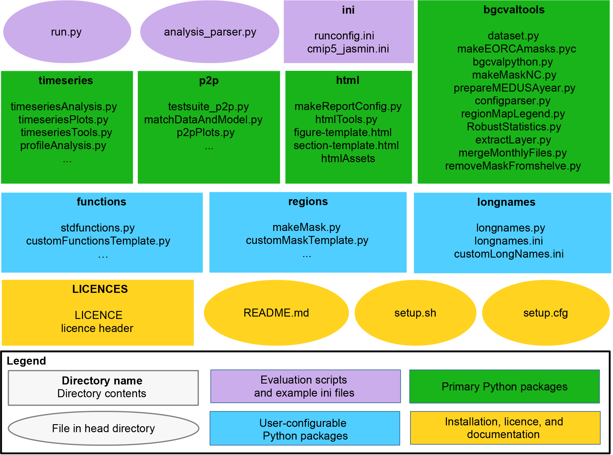
Figure 2 The structure of the BGC-val repository. The principal directories are shown as rectangles, with the name of the directory in bold followed by the key files contained in that directory. Individual files in the head directory are shown with rounded corners. The evaluation scripts and the configuration directory are shown in purple. The primary Python modules are split into four directories, shown in green rectangles. The three user-configurable Python modules are shown as blue rectangles. The licence, README, and setup files are shown in yellow.

In this figure, ovals are used to show single files in the head directory, and rectangles show folders or packages. In the top row of Fig. 2, there are two purple ovals and a rectangle which represent the important evaluation scripts and the example configuration files. These files include the run.py executable script, which is a user-friendly wrapper for the analysis_parser.py script (also in the head directory). The analysis_parser.py file is the principal Python file that loads the run configuration and launches the individual analyses. The ini directory includes several example configuration files, including the configuration files that were used to produce the figure in this document. Note that the ini directory is not a Python package, just a repository that holds several files. A full description of the functionality of configuration files can be found in Sect. 4.1.

The four main Python packages in BGC-val are shown in green rectangles in Fig. 2. Each of these modules has a specific purpose: the timeseries package described in Sect. 4.2.1 performs the evaluation of the time development of the model, the p2p package described in Sect. 4.2.2 does an in-depth spatial comparison of a single point in time for the model against a historical data field, and the html package described in Sect. 4.2.3 contains all the Python functions and html templates needed to produce the html summary report. This bgcvaltools package contains many Python routines that perform a range of important functions in the toolkit. These tools include, but are not limited to, a tool to read NetCDF files, a tool to extract a specific 2-D layer or transect, a tool to read and understand the configuration file, and many others.

The three user-configurable packages functions, regions, and longnames are shown in blue in Fig. 2. The functions package, described in Sect. 4.3.1, contains all the front-loading analysis functions described in Sect. 2.3, which are applied in the first stage of the evaluation process described in Sect. 3. The regions package described in Sect. 4.3.2 contains all the masking tools described in Sect. 2.4 and which are applied in the third stage of the evaluation process described in Sect. 3. The longnames package, described in Sect. 4.3.3, is a simple tool which behaves like a look-up dictionary, allowing users to link human-readable or “pretty” names (like “chlorophyll”) against the internal code names or shorthand (like “chl”). The pretty names are used in several places, notably in the figure titles and legends and on the html report.

The licences directory, the setup configuration files and the README.md are all in the main directory of the folder, as shown in yellow in Fig. 2. The licences directory contains information about the Revised Berkeley Software Distribution (BSD) three-clause licence. The README.md file contains specific details on how to install, set up, and run the code. The setup.py and setup.cfg files are used to install the BGC-val toolkit.

4.1 The configuration file

The configuration file is central to the running of BGC-val and contains all the details needed to evaluate a simulation. This includes the file path of the input model files, the user's choice of analysis regions, layers, and functions, the names of the dimensions in the model and observational files, the final output paths, and many other settings. All settings and configuration choices are recorded in an single file using the .ini format. Several example configuration files can also be found in the ini directory. Each BGC-val configuration file is composed of three parts: an active keys section, a list of evaluation sections, and a global section. Each of these parts is described below.

The tools that parse the configuration file are in the configparser.py module in the bgcvaltools package. These tools interpret the configuration file and use them to direct the evaluation. Please note that we use the standard .ini format nomenclature while describing configuration files. In this, [Sections] are denoted with square brackets, each option is separated from its value by a colon, “:”, and the semi-colon “;” is the comment syntax in .ini format.

4.1.1 Active keys section

The active keys section should be the first section of any BGC-val configuration file. This section consists solely of a list of Boolean switches, one Boolean for each field that the user wants to evaluate.

[ActiveKeys]
Chlorophyll     : True
A               : False
; B             : True

To reiterate the ini nomenclature, in this example ActiveKeys is the section name, and Chlorophyll, A, and B are options. The values associated with these options are the Booleans True, False, and True. Option B is commented out and will be ignored by BGC-val.

In the [ActiveKeys] section, only options whose values are set to True are active. False Boolean values and commented lines are not evaluated by BGC-val. In this example, the Chlorophyll evaluation is active, but both options A and B are switched off.

4.1.2 Individual evaluation sections

Each True Boolean option in the [ActiveKeys] section needs an associated [Section] with the same name as the option in the [ActiveKeys] section. The following is an example of an evaluation section for chlorophyll in the HadGEM2-ES model.

[Chlorophyll]
name             : Chlorophyll
units            : mg C/m^3

; The model name and paths
model            : HadGEM2-ES
modelFiles       : /Path/*.nc
modelgrid        : CMIP5-HadGEM2-ES
gridFile         : /Path/grid_file.nc

; Model coordinates/dimension names
model_t          : time
model_cal        : auto
model_z          : lev
model_lat        : lat
model_lon        : lon

; Data and conversion
model_vars       : chl
model_convert    : multiplyBy
model_convert_factor : 1e6
dimensions       : 3

; Layers and Regions
layers           : Surface 100m
regions          : Global SouthernOcean

The name and units options are descriptive only; they are shown on the figures and in the html report, but do not influence the calculations. This is set up so that the name associated with the analysis may be different to the name of the fields being loaded. Similarly, while NetCDF files often have units associated with each field, they may not match the units after the user has applied an evaluation function. For this reason, the final units after any transformation must be supplied by the user. In the example shown here, HadGEM2-ES correctly used the CMIP5 standard units for chlorophyll concentration, kg m⁻³. However, we prefer to view chlorophyll in units of mg m⁻³.

The model option is typically set in the Global section, described below in Sect. 4.1.3, but it can be set here as well. The modelFiles option is the path that BGC-val should use to locate the model data files on local storage. The modelFiles option can point directly at a single NetCDF file or can point to many files using wild cards (*, ?). The file finder uses the standard Python package glob, so wild cards must be compatible with that package. Additional nuances can be added to the file path parser using the placeholders $MODEL, $SCENARIO, $JOBID, $NAME, and $USERNAME. These placeholders are replaced with the appropriate global setting as they are read by the configparser package. The global settings are described below in Sect. 4.1.3. For instance, if the configuration file is set to iterate over several models, then the $MODEL placeholder will be replaced by the model name currently being evaluated.

The gridFile option allows BGC-val to locate the grid description file. The grid description file is a crucial requirement for BGC-val, as it provides important data about the model mask, the grid cell area, and the grid cell volume. Minimally, the grid file should be a NetCDF which contains the following information about the model grid: the cell-centred coordinates for longitude, latitude, and depth, and these fields should use the same coordinate system as the field currently being evaluated. In addition, the land mask should be recorded in the grid description NetCDF in a field called tmask, the cell area should be in a field called area, and the cell volume should be recorded in a field labelled pvol. BGC-val includes the meshgridmaker module in the bgcvaltools package and the function makeGridFile from that module can be used to produce a grid file. The meshgridmaker module can also be used to calculate the cross-sectional area of an ocean transect, which is used in several flux metrics such as the Drake Passage Current or the Atlantic meridional overturning circulation.

Certain models use more than one grid to describe the ocean; for instance, NEMO uses a U grid, a V grid, a W grid, and a T grid. In that case, care needs to be taken to ensure that the grid file provided matches the data. The name of the grid can be set with the modelgrid option.

The names of the coordinate fields in the NetCDF need to be provided here. They are model_t for the time and model_cal for the model calendar. Any NetCDF calendar option (360_day, 365_day, standard, Gregorian, etc.) is also available using the model_cal option; however, the code will preferentially use the calendar included in standard NetCDF files. For more details, see the num2date function of the netCDF4 Python package (https://unidata.github.io/netcdf4-python/, last access: 5 October 2018). The depth, latitude, and longitude field names are passed to BGC-val via the model_z, model_lat, and model_lon options.

The model_vars option tells BGC-val the names of the model fields that we are interested in. In this example, the CMIP5 HadGEM2-ES chlorophyll field is stored in the NetCDF under the field name chl. As already mentioned, HadGEM2-ES used the CMIP5 standard units for chlorophyll concentration, kg m⁻³, but we prefer to view chlorophyll in units of mg m⁻³. As such, we load the chlorophyll field using the conversion function multiplyBy and give it the argument 1e6 with the model_convert_factor option. More details are available below in Sect. 4.3.1 and in the README.md file.

BGC-val uses the coordinates provided here to extract the layers requested in the layers option from the data loaded by the function in the model_convert option. In this example that would be the surface and the 100 m depth layer. For the time series and profile analyses, the layer slicing is applied in the DataLoader class in the timeseriesTools module of the timeseries package. For the point-to-point analyses, the layer slicing is applied in the matchDataAndModel class in the matchDataAndModel module of the p2p package.

Once the 2-D field has been extracted, BGC-val masks the data outside the regions requested in the regions option. In this example, that is the Global and the SouthernOcean regions. These two regions are defined in the regions package in the makeMask module. This process is described below in Sect. 4.3.2.

The dimensions option tells BGC-val what the dimensionality of the variable will be after it is loaded, but before it is masked or sliced. The dimensionality of the loaded variable affects how the final results are plotted. For instance, one-dimensional variables such as the global total primary production or the total Northern Hemisphere ice extent cannot be plotted with a depth profile or with a spatial component. Similarly, two-dimensional variables such as the air–sea flux of CO₂ or the mixed layer depth should not be plotted as a depth profile, but can be plotted with percentile distributions. Three-dimensional variables such as the temperature and salinity fields, the nutrient concentrations, and the biogeochemical advected tracers are plotted with time series, depth profile, and percentile distributions. If any specific types of plots are possible but not wanted, they can be switched off using one of the following options.

makeTS          : True
makeProfiles    : False
makeP2P         : True

The makeTS option controls the time series plots, the makeProfiles option controls the profile plots, and the makeP2P option controls the point-to-point evaluation plots. These options can be set for each active keys section, or they can be set in the global section, as described below.

In the case of the HadGEM2-ES chlorophyll section, shown in this example, the absence of an observational data file means that some evaluation figures will have blank areas, and others figures will not be made at all. For instance, it is impossible to produce a point-to-point comparison plot without both model and observational data files. The evaluation of [Chlorophyll] could be expanded by mirroring the model's coordinate and convert fields with a similar set of data coordinates and convert functions for an observational dataset.

4.1.3 Global section

The [Global] section of the configuration file can be used to set default behaviour which is common to many evaluation sections. This is because the evaluation sections of the configuration file often use the same option and values in several sections. As an example, the names that a model uses for its coordinates are typically the same between fields; i.e. a chlorophyll data file will use the same name for the latitude coordinate as the nitrate data file from the same model. Setting default analysis settings in the [Global] section ensures that they do not have to be repeated in each evaluation section. As an example, the following is a small part of a global settings section.

[Global]
model           : ModelName
model_lat       : Latitude

These values are now the defaults, and individual evaluation sections of this configuration file no longer require the model or model_lat options. However, note that local settings override the global settings. Note that certain options such as name or units cannot be set to a default value.

The global section also includes some options that are not present in the individual field sections. For instance, each configuration file can only produce a single output report, so all the configuration details regarding the html report are kept in the global section.

[Global]
makeComp        : True
makeReport      : True
reportdir       : reports/HadGEM2-ES_chl

The makeComp is a Boolean flag to turn on the comparison of multiple jobs, models, or scenarios. The makeReport is a Boolean flag which turns on the global report making and reportdir is the path for the html report.

The global options jobID, year, model, and scenario can be set to a single value or can be set to multiple values (separated by a space character) by swapping them with the options jobIDs, years, models, or scenarios. For instance, if multiple models were requested, then swap

[Global]
model           : ModelName1

with the following.

[Global]
models          : ModelName1 ModelName2

For the sake of the clarity of the final report, we recommend only setting one of these options with multiple values at one time. The comparison reports are clearest when grouped according to a single setting; i.e. please do not try to compare too many different models, scenarios, and job IDs at the same time.

The [Global] section also holds the paths to the location on disc where the processed data files and the output images are to be saved. The images are saved to the paths set with the following global options: images_ts, images_pro, images_p2p, and images_comp for the time series, profiles, point-to-point, and comparison figures, respectively. Similarly, the post-processed data files are saved to the paths set with the following global options: postproc_ts, postproc_pro, and postproc_p2p for the time series, profiles, and point-to-point-processed data files, respectively.

As described above, the global fields jobID, year, model, and scenario can be used as placeholders in file paths. Following the bash shell grammar, the placeholders are marked as all capitals with a leading $ sign. For instance, the output directory for the time series images could be set to the following.

[Global]
images_ts : images/$MODEL/$NAME

$MODEL and $NAME are placeholders for the model name string and the name of the field being evaluated. In the example in Sect. 4.1.2 above, the images_ts path would become images/HadGEM2-ES/Chlorophyll. Similarly, the basedir_model and basedir_obs global options can be used to fill the placeholders $BASEDIR_MODEL and $BASEDIR_OBS such that the base directory for models or observational data does not need to be repeated in every section.

A full list of the contents of a global section can be found in the README.md file. Also, several example configuration files are available in the ini directory.

4.2 Primary Python packages

In this section, we describe the important packages that are shown in green in Fig. 2. The timeseries package is described in Sect. 4.2.1, the p2p package is described in Sect. 4.2.2, and the html package is described in Sect. 4.2.3. All the figures in Sect. 4.2 were produced on the JASMIN computational resource using the example configuration file ini/HadGEM2-ES_no3_cmip5_jasmin.ini, and the html summary report associated with that configuration file is available in the Supplement.

Outside the three main packages described below, the bgcvaltools package contains many Python routines that perform a range of important functions. These tools include a tool to read NetCDF files dataset.py, a tool to extract a specific 2-D layer or transect extractLayer.py, and a tool to read and understand the configuration file, configparser.py. There is a wide and diverse selection of tools in this directory: some of them are used regularly by the toolkit, and some are only used in specific circumstances. More details are available in the README.md file, and each individual module in the bgcvaltools is sufficiently documented that its role in the toolkit is clear.

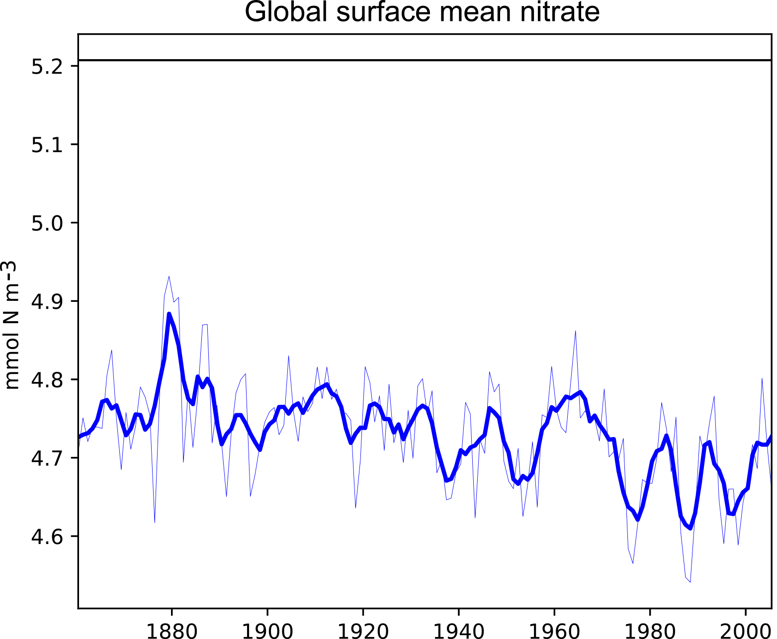
Figure 3 A plot produced by the time series package. This figure shows the time development of a single metric, in this case the global surface mean nitrate in HadGEM2-ES in the historical simulation. It also shows the 5-year moving average of the metric.

4.2.1 Time series tools

This timeseries package is a set of Python tools that produces figures showing the time development of the model. These tools manage the extraction of data from NetCDF files, the calculation of a range of metrics or indices, the storing and loading of processed data, and the production of figures illustrating these metrics.

Firstly, the time development of any combination of depth layer and region can be investigated with these tools. The spatial regions can be taken from the predefined list or a custom region can be created. The predefined regions are listed in the regions directory of the BGC-val. Many metrics are available including, mean, median, minimum, maximum, and all percentiles divisible by 10 (10th percentile, 20th percentile, etc.). Furthermore, any user-defined custom function can also be included as a custom function, for instance the calculation of global total integrated primary production or the total flux through the Drake Passage.

The time series tools produce three types of analysis plots. Examples of these three types of figures are shown in Figs. 3, 4, and 5. All three examples use annual averages of the nitrate (CMIP5 name: no3) in the surface layer of the global ocean in the HadGEM2-ES model historical scenario, ensemble member r1i1p1.

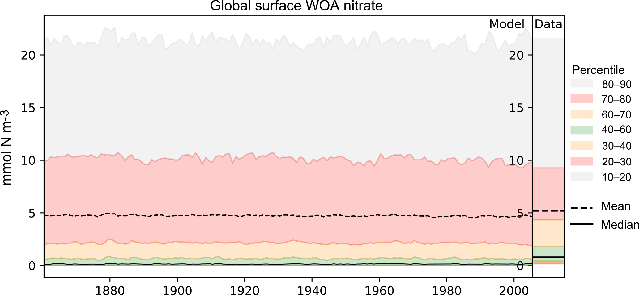
Figure 4 A plot produced by the time series package. The figure shows the time developers of many metrics at once: the mean, median, and several percentile ranges of the observational data and the model data. In this case, the model data are the global surface mean nitrate in HadGEM2-ES in the historical simulation.

Figure 5 A plot produced by the time series package. The figure shows the spatial distribution of the model (a) and the observational dataset (b). In this case, the model data are the global surface mean nitrate in HadGEM2-ES in the historical simulation.

Figure 3 shows the time development of a single variable: the mean of the nitrate in the surface layer over the entire global ocean. This figure shows the annual mean of the HadGEM2-ES model's nitrate as a thin blue line, the 5-year moving average of the HadGEM2-ES model's nitrate as a thick blue line, and the World Ocean Atlas (WOA) data (Garcia et al., 2013b) as a flat black line. The WOA data used here are an annual average climatological dataset and hence do not have a time component. This figure highlights the fact that the model simulates a decrease in the mean surface nitrate over the course of the 20th century.

Figure 4 shows an example of a percentile range plot, which shows the time development of the spatial distribution of the model data, including the mean and median, and coloured bands to indicate the 10–20, 20–30, 40–60, 60–70, and 70–80 percentile bands. This kind of plot also shows the percentile distribution of the spatial distribution of the observational data in a column on the right-hand side. Figure 4 shows the behaviour of nitrate in the surface layer over the entire global ocean, in the HadGEM2-ES model historical scenario, ensemble member r1i1p1. This type of plot is produced when the data have two or three dimensions but cannot be produced for one-dimensional model datasets. The percentile figures can be produced for any layer and spatial region and these metrics are all area weighted. For all three kinds of time series figures, a real dataset can be added, although it is not possible to include the time development of the observational dataset at this stage.

The time series package also produces a figure showing the spatial distribution of the model and observational data. Figure 5 shows an example of such a figure, in which panel (a) shows the spatial distribution of the final time step of the model, and panel (b) shows the spatial distribution of the observational dataset. It is possible to plot data for any layer for any region. These spatial distributions are made using the Plate Carré projection, and the projections are set to focus on the region in question. Figure 5 highlights the fact that the HadGEM2-ES model failed to capture the high nitrate seen in the observational data in the equatorial Pacific.

BGC-val can also produce several figures showing the time development of the model datasets over their entire water columns. The profile modules are stored in the timeseries package, as the time series and profiles figures share many of the same underlying methods. Figures 6, 7, and 8 are examples of three profile plots showing the time development over the water column of the global mean nitrate in the HadGEM2-ES model historical simulation, ensemble member r1i1p1. These plots can only be produced when the data have three dimensions. These plots can be made for any region from the predefined list or for custom regions.

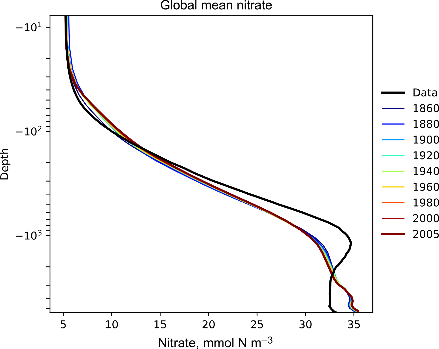
Figure 6 The time development of the global mean dissolved nitrate over a range of depths. This figure shows the HadGEM2-ES global mean nitrate over the entire water column; each model year is included as a coloured line, and the annual mean of the World Ocean Atlas nitrate climatology dataset is shown as a black line.

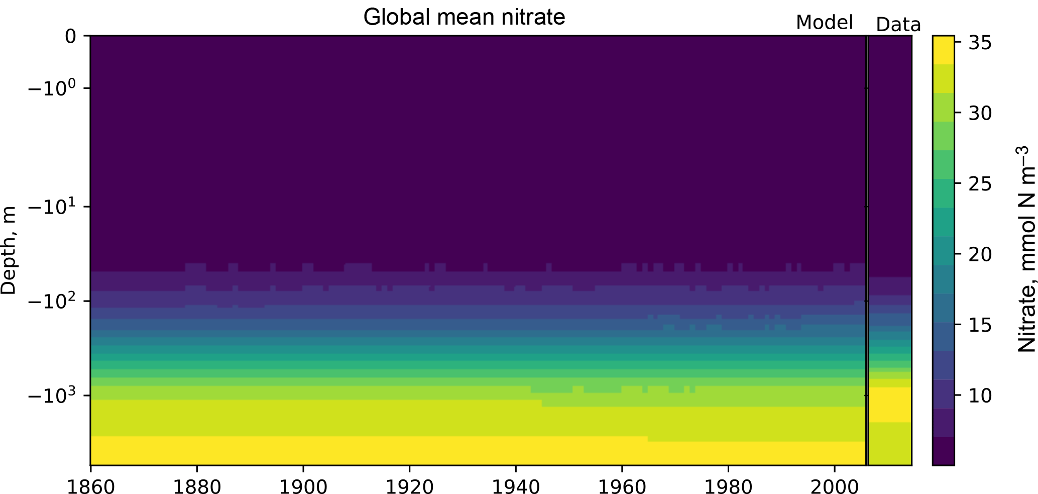
Figure 7 The time development of the global mean dissolved nitrate over a range of depths. The figure shows the same data as Fig. 6, but as a Hovmöller time series plot. The annual mean of the World Ocean Atlas nitrate climatology dataset is shown as a column on the right-hand side of the figure.

Figure 8 The time development of the global mean dissolved nitrate over a range of depths. The figure shows the same data as Figs. 6 and  7, but with the World Ocean Atlas nitrate observational measurement subtracted from the model time series.

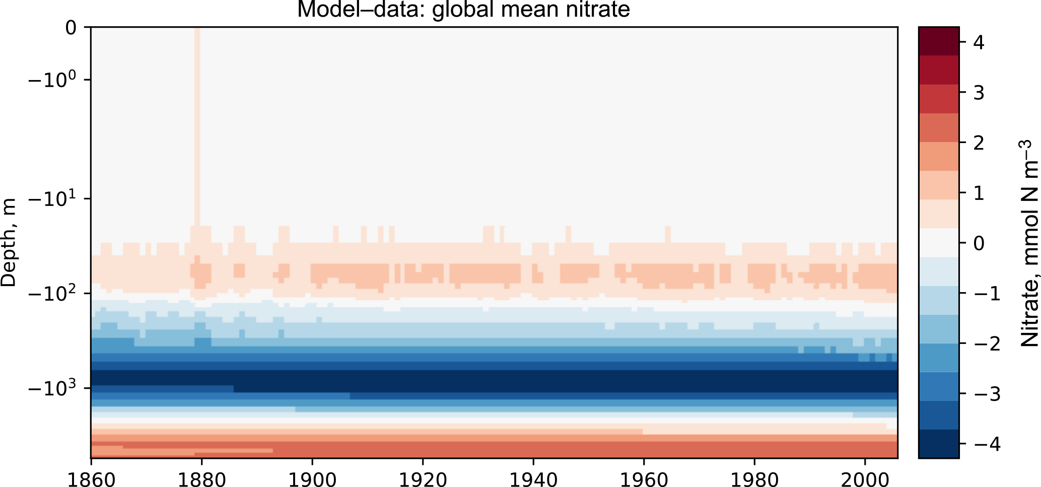
Figure 6 shows the time development of the depth profile of the model and observational data. The x axis shows the value, in this case the nitrate concentration in mmol N m⁻³ and the y axis shows depths. These types of plots always show the first and last time slice of the model, then a subset of the other years is also shown. Each year is assigned a different colour, with the colour scale shown in the right-hand side legend. If available, the observational data are shown as a black line. This figure shows the annual mean of the World Ocean Atlas nitrate climatology dataset as a black line.

Figures 7 and 8 are both Hovmöller diagrams (Hovmöller, 1949) and they show the depth profile over time for model and observational data. Figure 7 shows the model and the observational data side by side, and Fig. 8 shows the difference between the model data and the observational data. The Hovmöller difference diagrams are only made when an observation dataset is supplied. There appears to be a peak in the difference between the model and the observations over the entire water column in the year 1880. This does not appear to be a fault in the model, but simply a brief period during which the difference was slightly larger than zero. This peak in the mean is also visible in the global mean surface nitrate in Fig. 3, but is not visible in the percentile distribution of the surface nitrate in Fig. 4.

Figures 6, 7, and 8 all show that the model data match the observational nitrate near the surface, but diverge at depth. The model underestimates the peak in the global mean of the observational nitrate at a depth of approximately 1000 m and then overestimates the observed nitrate below 2000 m. Also, the model does not show much interannual variability in the structure of the global annual average nitrate over the 145-year simulation. However, it is unclear from the WOA annual average whether we should expect any variability from the model over this time range.

In the timeseries package, there is also a set of tools for comparing the time series development between multiple versions of the same metric. This is effectively the same as plotting several versions of Fig. 3 on the same axes. This kind of diagram can be useful to compare the same measurement between different regions, depth layers, or different members of a model's ensemble. However, these plots can also be used to compare multiple models. Several example figures are included in Sect. 5.

4.2.2 Point-to-point model–data comparison tools

In addition to the time series evaluation, BGC-val can perform a direct point-to-point comparison of model against data. The point-to-point tools here are based on the work by de Mora et al. (2013). In that work, we demonstrated that using point-to-point analysis is more representative of a real marine dataset than comparing the bulk mean of the model to the bulk mean of the data. The method involves matching the model data to the closest corresponding observational measurement, then hiding all model points which do not have a corresponding observational measurement and vice versa. The point-to-point methodology means that the model and observational data have not be re-interpolated to a common grid: they both retain their original grid description.

Figures 9, 10, and 11 show examples of the figures made by the point-to-point package. In all three figures, the model data are the global surface nitrate in HadGEM2-ES in the historical simulation in ensemble member r1i1p1 in the year 2000. The observational data come from the nitrate dataset in the World Ocean Atlas (Garcia et al., 2013b).

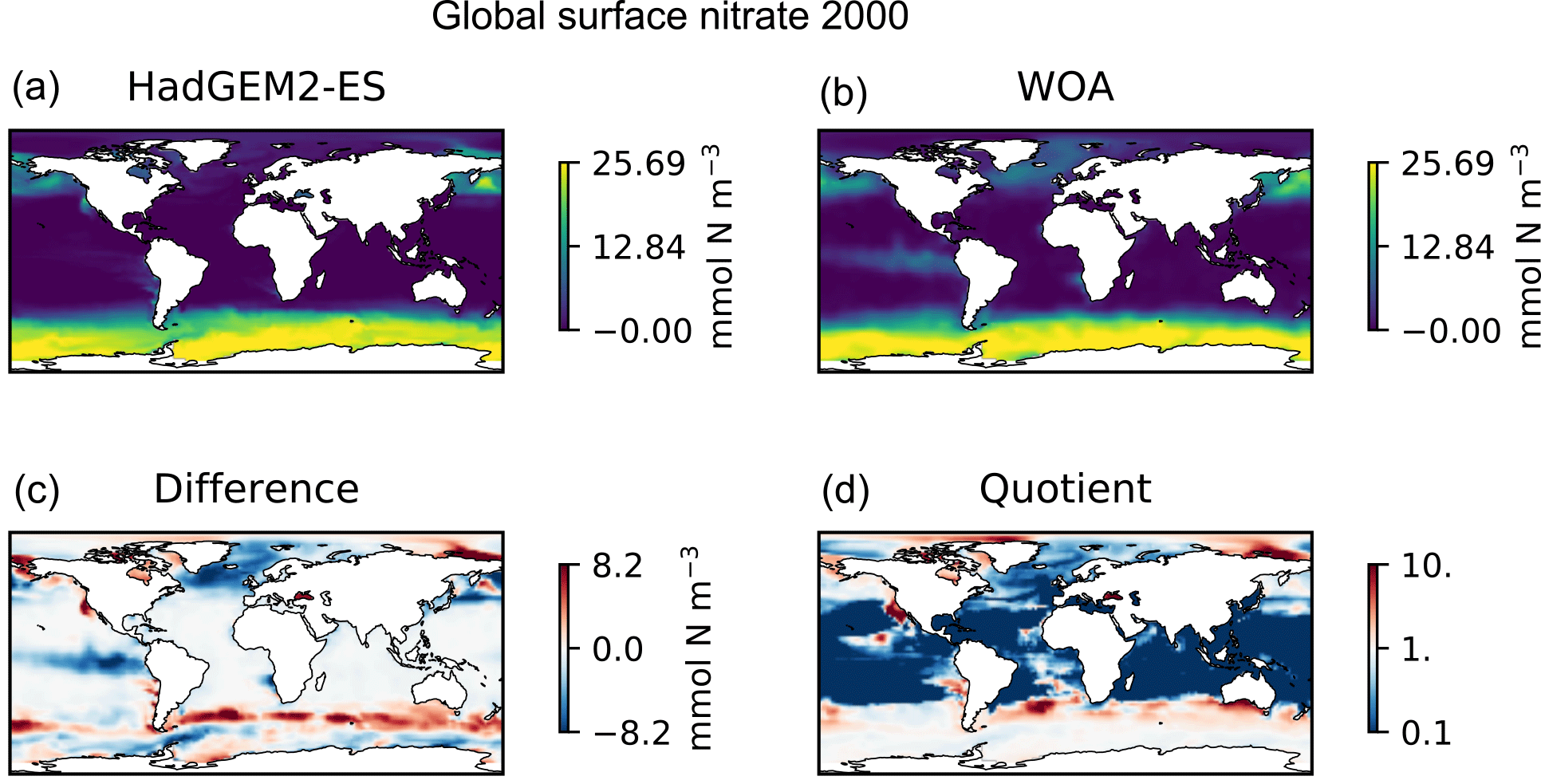
Figure 9 Four spatial distributions showing the model (a), the observational data (b), the difference between them (c), and their quotient (d). The model data in these plots are the global surface nitrate in HadGEM2-ES in the historical simulation in ensemble member r1i1p1 in the year 2000. The observational data come from the annual nitrate dataset in the World Ocean Atlas.

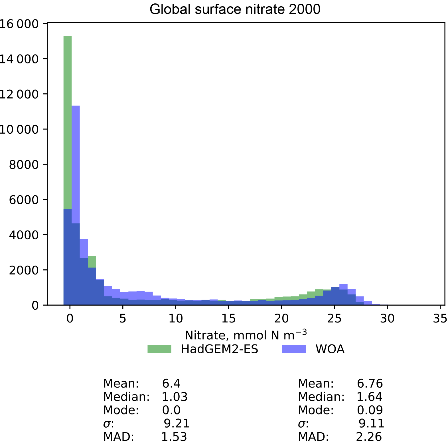
Figure 10 A pair of histograms showing the model (green) and the observational data (blue), as well as some metrics of the distribution shape. The model data are the global surface nitrate in HadGEM2-ES in the historical simulation in the year 2000. The observational data come from the nitrate dataset in the World Ocean Atlas. The metrics are the mean, median, the mode, the standard deviation, σ, and the median absolute deviation (MAD).

Figure 9 is a group of four spatial distributions comparing the model and observational datasets. The map in Fig. 9a is the model, Fig. 9b is the observations, Fig. 9c is the difference between the model and observations (model minus observational data), and Fig. 9d is the quotient (model over observational data). This example shows the comparison at the ocean surface, but these tools also allow for longitudinal or latitudinal transect comparisons or a spatial distribution along a specific depth level. This figure shows that the year 2000 of the HadGEM2-ES model reproduces the large-scale spatial patterns seen in the observational dataset. The model has significantly higher nitrate that the observational climatology in the Southern Ocean, the North Pacific, and the equatorial regions and has significantly lower nitrate in the Arctic regions. A discrepancy in the spatial extent of the high nitrate in the Southern Ocean is shown clearly in the difference panel of this figure. The quotient panel of this figure also shows that model underestimates the low-nitrate regions around the tropical waters.

Figure 10 is a pair of histograms showing the same model and observational data as in Fig. 9. This figure also shows some measures of the central tendency (mean, median, mode) and measures of the deviation (standard deviation and median absolute deviation) for both model and data. These histograms confirm that the model underestimates the nitrate concentration in the low-nitrate region, which covers a significant region and is the mode of the WOA dataset.

Figure 11 shows the distribution of the model and the observational data with the model data along the x axis and the observation data along the y axis. The 1:1 line is shown as a dashed line; the model overestimates the observation to the right of this line and underestimates it to the left of this line. A linear regression is shown as a full line, with the slope, intersect, P value, correlation, and number of data points shown on the right-hand side of the figure. In this example, the linear regression is very close to the 1:1 line, and the bulk of the data is close to a good fit. While the model reproduces the distribution of observational data at low values and high nitrate concentrations, the model overestimates more than half of the nitrate observations between 10 and 20 mmol N m⁻³.

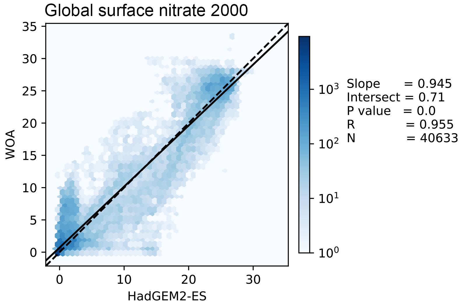
Figure 11 This figure shows the distribution of the model and the observational data with the model data along the x axis and the observation data along the y axis. The model data are the global surface nitrate in HadGEM2-ES in the historical simulation in the year 2000. The observational data come from the nitrate dataset in the World Ocean Atlas. The 1:1 line is shown as a dashed line. A linear regression is shown as a full line, with the slope, intersect, P value, correlation, and number of data points shown on the right-hand side.

4.2.3 HTML report

The html package of the BGC-val toolkit contains all the tools needed to produce a report summarising the output of the time series, the profile, and the point-to-point packages. The principal file in this package is the makeReportConfig module, which produces an html document according to the settings of the configuration file. Using the configuration file, the report maker finds all the images and uses several template files to stitch together the individual sections of the report. The html is based on a template taken from https://html5up.net/ (last access: 5 October 2018), used under the Creative Commons Attribution 3.0 License.

An example of the HTML report is available in the Supplement. This report shows the output of the example configuration file: ini/HadGEM2-ES_no3_cmip5_jasmin.ini. In order to access this report, please download and unzip the files, then export them to a local copy before opening the index.html file in a browser of your choice.

4.3 User-configurable Python packages

In this section, we look at the code behind the extensive customisability of BGC-val: the functions, regions, and longnames packages shown in blue in Fig. 2 are described in this section. The functions package is described in Sect. 4.3.1, the regions package is described in Sect. 4.3.2, and the longnames package is described in Sect. 4.3.3.

4.3.1 Functions

The functions package is a significant contributor of the flexibility of BGC-val. This package allows any operation to be applied to a dataset as the data are loaded. In most cases, the conversion is one of the standard functions such as multiply or divide by some arbitrary number, add a constant value to the variable, or simply just load the data as is with no conversion. However, this package can also be used to perform complex data processing.

The data_convert and model_convert options in the configuration file allow BGC-val to determine which function to apply to the model or observational data as they are loaded. There is no default function, so to simply load the data into the file, the standard function NoChange should be specified in the data_convert or model_convert options.

As an example of the structure of a basic function, we look at a simplified version of the multiplyBy function in the stdfunctions module of the functions package.

def multiplyBy(nc,keys, **kwargs):
  f = float(kwargs['factor'])
  return nc.variables[keys[0]][:]*f

After declaring the function name and arguments in the first line, this function loads the factor from the keyword arguments (kwargs) and parses it into the single precision floating format in the second line. In the third line, this function loads the first item in the keys list from the NetCDF dataset nc, then multiplies that data by the factor f, and returns the product. The path to the NetCDF file, the choice of function, the list of keys, and the factor are all provided by the configuration file.

All functions need to be called with the same arguments: nc is a NetCDF file opened by the dataset module from the bgcvaltools package. The keys argument is a list of strings which represent the names of fields in a NetCDF file, and the optional kwargs argument is used to pass any extra information that is needed (such as a factor or addend).

The keyword arguments which are passed to the function must be preceded by the text model_convert_ or data_convert_ strings in the configuration file. In the example above, the “factor” was written in the configuration file as

 model_convert_factor : 1e6

but it was loaded in the multiplyBy function as kwargs['factor'].

Some evaluation metrics require multiple variables to be loaded at once and combined together. The stdfunctions module of the functions package contains a few such medium-complexity operations, such as “sum”, which returns the sum of the fields in the keys list. The 'divide' function returns the quotient of the first key over the second key from the keys list.

More complex functions can be implemented as well, for instance depth integration, global totals, or the flux through a certain cross section. There are several examples of complex functions in the functions folder. Note that some of these functions can change the dimensionality of the data, and caution needs to be taken to ensure that the dimensions option in the configuration file matches the dimensions of the output of this function.

4.3.2 Regions

Similarly to the functions package described above, the regions package allows for expanded flexibility in the evaluation of models. The term “region” here is a portmanteau for any selection of data based on their coordinates or values. Typically, these are spatial regional cuts, such as “Northern Hemisphere”, but the masking is not limited to spatial regions. For instance, the regions package can also be used to remove negative values and to remove zero, NaN, or inf values.

As an example of the structure of a basic regional mask, we look at the SouthHemisphere region in the makeMask module of the regions package.

def SouthHemisphere(
     name,region,
     xt,xz,xy,xx,xd):
  a = np.ma.masked_where(xy>0.,xd)
  return a.mask

The Python standard package NumPy has been imported as np. Each regional masking function has access to the following fields: name, the name of the data; region, the name of the regional cut; xt, a one-dimensional array of the dataset times; xz, a one-dimensional array of the dataset depths; xy, a one-dimensional array of the dataset latitudes; xx, a one-dimensional array of the dataset longitudes; and xd, a one-dimensional array of the data. The second to last line creates a masked array of the data array which is masked in all the places where the latitude coordinate is greater than zero (i.e. the Northern Hemisphere). The final line returns the mask for this array. All region extraction functions return a NumPy mask array. In Python, NumPy masks are an array of Booleans in which “true” is masked.

Many regions are already defined in the file regions/makeMask.py, but it is straightforward to add a new region using the template file regions/customMaskTemplate.py. To do this, make a copy of the regions/customMaskTemplate.py file in the regions directory, rename the function and file to your mask name, and add whatever cuts are required. BGC-val will be able to locate your region, provided that the region name matches the Python function and the region in your configuration file.

4.3.3 Long names

In the Python source code, objects are often abbreviated or labelled with shorthand, and spaces and hyphens are not acceptable in object names. This means that the internal name of a model, dataset, field, layer, or region is not usually the same in the text that we want to appear in public plots. For this reason, the long name package has a dictionary of common terms with their abbreviated name linked to a “pretty” name. The dictionary has definitions for each model, scenario, dataset, object, mask, cut, region, field, and other pythonic object used in BGC-val. These pretty names are used when preparing outwards-facing graphics and html pages such that the name of an object in the configuration file is not a source of confusion.

This package uses the standard configuration (ini) format for the dictionary. The custom long names configuration file is simply a long list of short names as the option and long names as the value. For example, the longnames.ini includes the following lines.

 no3     : Nitrate
 chl     : Chlorophyll

This means that we can label nitrate internally as “no3” as the evaluation name in our configuration file, but when it appears in plots, it will be shown as “nitrate”. Also note that the options are not case sensitive, but the values are case sensitive. While the default long name list is already relatively extensive, users can add their own long names to the longnames/customLongNames.ini file.

5 Applying BGC-val to CMIP5 RCP8.5

In this section, we show some example figures of the intercomparison of several CMIP5 models. These examples were produced using CMIP5 data on the JASMIN data processing facility (http://www.jasmin.ac.uk, last access: 5 October 2018), and the configuration file used to produce these is supplied in the BGC-val Git repository under the name cmip5_rcp85_jasmin.ini in the ini directory. The examples that we show here are the Atlantic meridional overturning circulation in Fig. 12, the Antarctic circumpolar current in Fig. 13, the total annual air to sea flux of CO₂ in Fig. 14, the total annual marine primary production in Fig. 15, and the global mean surface chlorophyll in Fig. 16. All five figures here show the 5-year moving average instead of the monthly or annual time resolution of the field in order to improve clarity. The 5-year window moving average is calculated using the mean of 2.5 years on either side of a central point. This means that the start and end points of the time series are the mean of only 2.5 years.

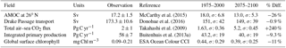
Table 1 shows the observational measurement for the multi-model mean of the years 1975–2000 in the historical scenario, the multi-model mean of the years 2075–2100 under the RCP8.5 scenario, and the percentage of change between 2075–2100 and 1975–2000 for all five fields.

These examples compare a subset of the CMIP5 models in the historical time range and RCP8.5 scenario in the ensemble member r1i1p1. The historical and RCP8.5 simulations are aligned such that the historical simulation links to the RCP scenario at the year 2005. This was done using the jasmin_cmip5_linking.py module in the bgcvaltools package.

The CMIP5 models shown in these figures are CESM1-BGC, CMCC-CESM, GFDL-ESM2G, GFDL-ESM2M, GISS-E2-H-CC, GISS-E2-R-CC, HadGEM2-CC, HadGEM2-ES, IPSL-CM5A-MR, IPSL-CM5B-LR, MPI-ESM-LR, MPI-ESM-MR, and NorESM1-ME. This report does not include all CMIP5 models, but rather a small number of examples of marine circulation and biogeochemistry metrics over the historical and RCP8.5 scenarios. The selection criterion was that the model was required to have biogeochemical datasets in the British Atmospheric Data Centre (BADC) archive of the CMIP5 data. The BADC is a UK mirror of the CMIP5 data archive, which is managed by the Centre for Environmental Data Analysis (CEDA), and this archive is accessible from the JASMIN data processing facility. We also required the r1i1p1 job identifier and the “latest” model run tag.

Using these tools, we uncovered a previously undetected error in the HadGEM2-ES RCP8.5 r1i1p1 simulation. The HadGEM2-ES RC8.5 r1i1pi simulation contains 2 years in which the annual mean data were produced without all 12 months. This made the two erroneous years differ significantly from the other years in our time series plots. After informing the HadGEM2-ES project manager, we were advised to substitute the r2i1p1 simulation in place of the HadGEM2-ES r1i1p1 simulation.

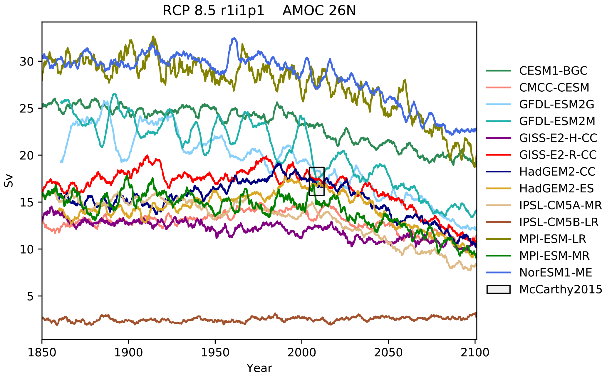
Figure 12 The Atlantic meridional overturning circulation at 26^∘ N in a subset of CMIP5 models. Each model is shown as a full line, and the historical measurement is shown as a grey area. The model data are a 5-year moving average.

Figure 13 The Drake Passage Current. Each model is shown as a full line, and the historical measurement is shown as a grey area. The model data are a 5-year moving average.

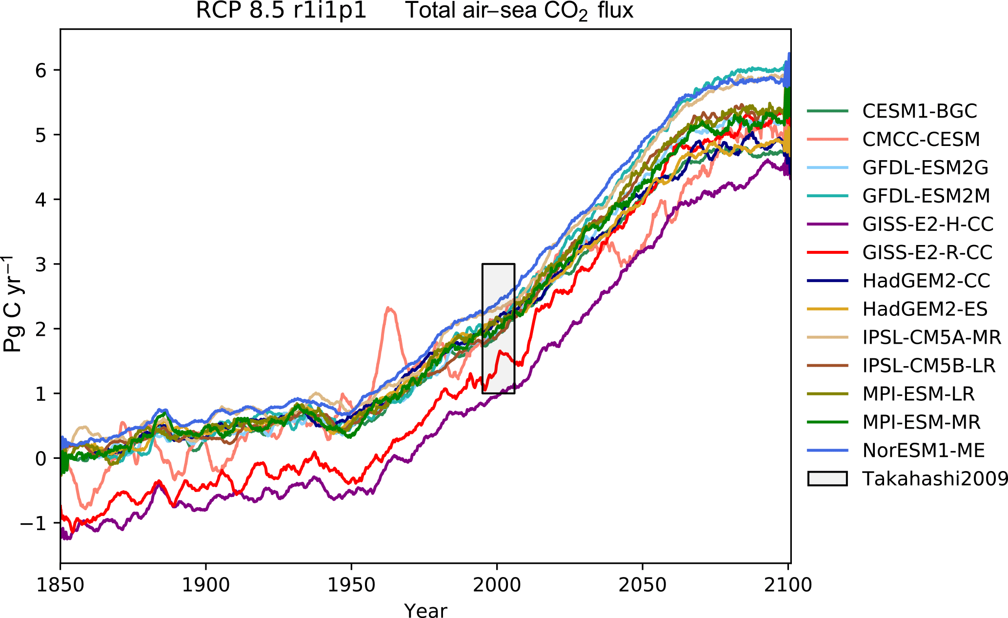
Figure 14 The total annual flux of CO₂ from the air to the sea in Pg yr⁻¹ under the RCP8.5 scenario

Figure 15 The total annual marine primary production of a range of models.

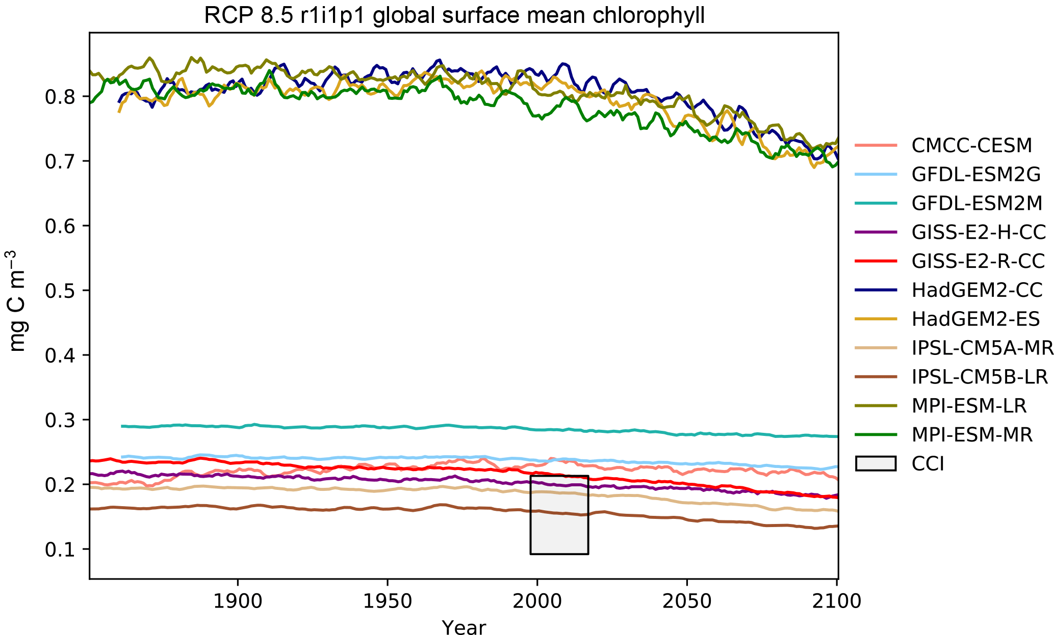
Figure 16 The global mean chlorophyll concentration for the surface layer of a range of CMIP5 models.

McCarthy et al. (2015)Donohue et al. (2016)Takahashi et al. (2009)Buitenhuis et al. (2013a)

Table 1 Summary table showing the multi-model mean and standard deviation of the five fields. After the field and units columns, the observational range, measurement uncertainty, and reference are shown. The fifth column shows the multi-model mean of years 1975–2000 and the standard deviation (σ) in the historical simulation. The sixth column shows the multi-model mean of years 2075–2100 and the standard deviation in the RCP8.5 simulation. The final column (% Diff.) shows the percentage of difference between the first period and the second period.

The Atlantic meridional overturning circulation (AMOC) is a major current and consists of two parts: a northbound transport between the surface and approximately 1200 m and a southbound transport between approximately 1200 and 3000 m (Kuhlbrodt et al., 2007). The AMOC is responsible for the production of roughly half of the ocean's deep waters (Broecker, 1991). The northward heat transport of the AMOC is substantial and has a significant role in the climate of the Northern Hemisphere. The strength of the northbound AMOC in several CMIP5 models was shown in Fig. 12.35 of the IPCC report (Collins et al., 2013). The BGC-val toolkit was able to reproduce the AMOC analyses of the IPCC. As in the IPCC figure, Fig. 12 shows the historical and RCP8.5 projections of the AMOC produced by BGC-val. Please note that we use a different subset of CMIP5 models in this figure relative to IPCC Fig. 12.35. The RAPID array measured the long-term mean of the AMOC to be 17.2±1.5 Sv between 2004 and 2013 (McCarthy et al., 2015). This figure is shown as a black rectangle with a grey background in Fig. 12. The calculation was initially based on the methods used in the UK Met Office's internal ocean evaluation toolkit, Marine Assess, which uses the calculation described in Kuhlbrodt et al. (2007) and McCarthy et al. (2015). However, we have since expanded the original Marine Assess method to be model and grid independent. This cross-sectional area for the 26^∘ N transect was calculated and saved to a NetCDF file using the meshgridmaker module in the bgcvaltools package. The model-specific cross-sectional area was used to calculate the maximum of the depth-integrated cross-sectional current in the custom function cmip5AMOC in the circulation module in the functions package. Amongst the CMIP5 models that included a biogeochemical component, several models overestimated the AMOC, and several underestimated the AMOC in the historical simulation. However, nearly all simulations predict a decline in the AMOC over the 21st century, and the multi-model mean drops by 26 % from 18 Sv in the mean of the years 1975–2000 to 13 Sv in the mean of the years 2075–2100 under the RCP8.5 scenario.

The Antarctic Circumpolar Current (ACC) is a major current which has a significant impact on the climate of the Southern Ocean and Antarctica. The ACC flows eastward around Antarctica and is the dominant feature of the circulation of the Southern Ocean. The ACC was recently measured through the Drake Passage at 173.3±10.7 Sv (Donohue et al., 2016), making the ACC the strongest ocean current in the world. A metric to describe the ACC is the total volume transport through the narrow gap between South America and Antarctica, known as the Drake Passage, shown in Fig. 13. Here, the Drake Passage Current is calculated as the total depth-integrated current between the South American coast and the Antarctic peninsula along a line of constant longitude at 78^∘ W. To perform this calculation in a grid-independent way, a north–south line was drawn along 78^∘ W through each model grid cell there. As in the calculation of the AMOC, described above, this calculation was initially based on the methods used by the Met Office's internal ocean evaluation toolkit, Marine Assess, which uses the calculation described in Donohue et al. (2016). Like the AMOC calculation, we expanded the Marine Assess method to be model and grid independent. The length of the intersecting line between this line and each grid cell along the line was calculated, then multiplied by the thickness of the layer and the eastbound current. These products were summed together to produce the Drake Passage Current shown in Fig. 13. This cross-sectional area is calculated and saved to a NetCDF file using the meshgridmaker module in the bgcvaltools package. The calculation was performed in the custom function cmip5DrakePassage in the circulation module in the functions package. Figure 13 shows a moving average with a 5-year window for several CMIP5 models between the years 1860 and 2100 in units of Sverdrups and the observation of 173.3±10.7 Sv from Donohue et al. (2016). Several CMIP5 models make estimates of the Drake Passage transport within the uncertainty of the observational measurement. The percentage of difference between the multi-model means of 1975–2000 and 2075–2100 under the RCP8.5 scenario is a decrease of 0.9 %, even though the inter-model spread is particularly large (70–250 Sv).

The ocean is a major sink of CO₂ and absorbed approximately 27 % of anthropogenic CO₂ emissions between 2002 and 2011 (Le Quéré et al., 2013). The total air–sea flux of CO₂ from the atmosphere to the ocean is an important metric for understanding the fate of greenhouse gases (Takahashi et al., 1997). The total global air to sea flux of CO₂ from various CMIP5 models is shown in Fig. 14 and the observational range of 2±1 Pg C yr⁻¹ for the year 2000 is taken from Takahashi et al. (2009). Note that the observational data were recorded between 1970 and 2007, but scaled to the year 2000. The calculation was performed in the custom function TotalAirSeaFluxCO2 in the AirSeaFluxCO2 module in the functions package. The historical period shows a rise in the absorption of CO₂ between 1860 and 2005, and that trend is projected to continue into the future under the RCP8.5 scenario. The multi-model annual mean for the years 1975–2000 was 1.63 Pg of carbon per year, but rose by 240 % up to 5.2 Pg of carbon per year for the years 2075–2100.

The integrated primary production is the global sum of the primary production in the ocean. Marine phytoplankton are responsible for 56±7 Pg of primary production per year (Buitenhuis et al., 2013a), which is of similar magnitude to that of land plants (Field et al., 2011). The total primary production is an indicator of the strength of the base of the food chain. Changes in primary production may indicate severe impacts of climate change (Anav et al., 2013; Chavez et al., 2011). In order to calculate this value, we multiply the primary production from each grid cell by the volume of that grid cell, then take the global sum over the entire ocean. The calculation was performed in the custom function TotalIntPP in the TotalIntPP module in the functions package. Figure 15 shows a wide range of behaviours for the CMIP5 models. Some models show relatively consistent marine primary production, and some models show constant historical primary production, followed by a decrease in primary production going into the 21st century. One model, CMCC-CESM, even shows an increase in the 20th followed by a decrease in the 21st century. The multi-model mean annual primary production for the years 1975–2000 was 43.2 Pg of carbon per year, but decreased by 9 % down to 39.7 Pg of carbon per year for the years 2075–2100.

The concentration of chlorophyll in the surface of the ocean is a indicator of the quantity of phytoplankton in the waters. The global mean surface chlorophyll for the CMIP5 models (excluding the CESM1-BGC and NorESM1-ME models) is shown in Fig. 16. The observational data shown in Fig. 16 and in the chlorophyll row of Table 1 are from the ESA Ocean Colour Climate Change Initiative (CCI). The CCI data are taken from the Ocean Colour Climate Change Initiative dataset version 3.1, available online at http://www.esa-oceancolour-cci.org (last access: 5 October 2018). The model value for global mean surface chlorophyll was calculated by taking the 5-year moving average of the time series of the area-weighted mean of the surface layer for each CMIP5 model. To convert the model data into mg Chl m⁻³, we used the standard function multiplyBy with a multiplicand of 1e6 from the stdfunctions module in the functions package. The CCI global mean surface chlorophyll ranges from 0.09 to 0.21 mg Chl m⁻³ for the years 1997 to 2017. Note that this value represents the range of monthly means and was extracted using the ocean colour data portal https://www.oceancolour.org/portal/ (last access: 5 October 2018). This value is taken from remote sensing satellite measurements and does not have consistent coverage due to cloud cover and low light in the winter in the polar regions. The multi-model area-weighted mean surface chlorophyll for the years 1975–2000 was 0.44 mg Chl per cubic metre, but decreased by 11 % down to 0.39 mg of chlorophyll per cubic metre for the years 2075–2100. There appear to be two modes of behaviour in the chlorophyll of the CMIP5 models. The first grouping seems to overestimate the total chlorophyll and the second group is closer to the observed value from ESA Ocean Colour CCI.

The computational cost required to perform these evaluations depends on several factors, including the number of models being investigated, the number of years being investigated, the size of the model grid, the number of depth fields, the number of metrics requested, the number of regions requested, the number of depth layers requested, the number of fields under investigation, and the power of the computational system being used. To give a coarse estimate of the computational cost of the tool, we ran a single thread of BGC-val over a single model (HadGEM2-ES), for a single CMIP5 field (NO₃), over a single layer (surface), in a single region (global), over the entire CMIP5 historical period (1850–2007) and ran the time series, profile maker, a point-to-point comparison, and the html report maker. We used the JASMIN sci1 processing node, and ran three iterations. The average “wall-clock” time needed to run all evaluation metrics, produce all plots, and make the final html report was 5 min 39 s, and the peak memory usage (resident set size) was around 4 GB, as reported by the Linux utility time. This individual process can be parallelised such that several threads (usually different fields) can be run at once. Due to the time-saving tools described in Sect. 2.5, running the same evaluation a second time only took 4 to 5 s.

6 Conclusions

The biogeochemical evaluation toolkit, BGC-val, is a model- and grid-independent toolkit that has been built to evaluate marine biogeochemical models using a simple interface. We have presented the ideas that motivated the development of the BGC-val software framework, introduced the code structure, and shown some applications of the toolkit using model results from CMIP5.

We hope that we have successfully communicated the power and flexibility of this toolkit for the automation of marine model evaluation. This toolkit has already been deployed operationally to evaluate the spin-up phase of the marine component of the UKESM1. In the future, the authors will continue to develop and apply the toolkit outlined in this work. Furthermore, as it is straightforward to add new fields and model comparisons to BGC-val, we intend to continue to use this toolkit to compare UKESM1 and the other models submitted to CMIP6 against each other and against the CMIP5 models.

In addition, the framework that produces these figures was built to make it straightforward to load, mask, and compare model and observations, as well as share results. There are several potential expansions; for instance, it may be interesting to evaluate the production of emergent features in marine biogeochemical models based on the work of de Mora et al. (2016). Another feature which is currently under development is the production of pattern statistics diagrams, such as Taylor and target diagrams (Jolliff et al., 2009; Taylor, 2001).

While ESMValTool is a separate toolkit, many of the evaluation metrics used in BGC-val are also planned to be ported onto the ESMValTool (Poloczanska et al., 2016) platform by the authors of this paper. When ported into ESMValTool version 2, these metrics will be made available for use by the wider Earth system model evaluation community.

Appendix A: Installing and running BGC-val

Specific and up-to-date details on how to install, set up, and run the code can be found in the README.md file in the code repository. However, in this appendix, we present a bare-bones guide on how to use the BGC-val toolkit.

BGC-val was written to be compatible with Python 2.7 and has only been tested in a Linux environment. It requires several standard Python packages, including matplotlib, netCDF4, NumPy, and SciPy. It also requires a small number of nonstandard packages, such as the UKMO's cartopy package.

While the BGC-val code is available via the Zenodo service (de Mora et al., 2018), this is a snapshot and cannot be changed once it is published. The up-to-date versions of this repository will be available only with the GitLab service. For this reason, we recommend using the GitLab version instead of the Zenodo version. Instructions on how to register and access the toolkit can be found above in the “Code availability” section. The registration process will create a user account for you, and your account will be added to the BGC-val users group. Once registered, the repository can be cloned using the standard Git methodology.

Git clone git@gitlab.em.pml.ac.uk:
BGC-val-users/bgc-val.git

However, note that this address may differ in the future.

Once cloned, the BGC-val repository can be installed using the standard Python package installer, pip.

 pip install --user bgc-val-public

This will make the tools available in the user's Python working space.

To run the code, we advise users to make a copy of the relevant configuration file in the ini directory. Their local copy of the configuration file should then be edited as described in Sect. 4.1 to reflect their local evaluation requirements.

The BGC-val toolkit is launched by the following command.

run.py configuration.ini

run.py is a simple wrapper that passes the local configuration file as a command line argument to the main script, analysis_parser.py.