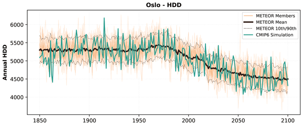
METEORv1.6: Spatial climate variability and integrated impact emulation

Climate impact assessment increasingly requires spatially explicit projections with realistic temporal variability at sub-annual resolution. METEORv1.6 extends the established METEOR spatial multi-timescale, multi-forcer climate emulation framework with two major capabilities: (1) a monthly climate variability model that generates realistic sub-annual climate sequences with seasonal cycles and inter-annual variability, enabling the generation of ensemble projections and (2) a modular impact assessment framework that translates climate projections into impact metrics. The monthly climate model represents seasonal harmonics and noise, while preserving covariance structures from the source model. Seasonal cycles are represented through harmonic analysis with temperature-dependent parameterization, enabling non-stationary simulation of seasonal timing shifts under warming. Principal Component Analysis is used to decompose monthly anomalies into spatial modes, then their temporal evolution and climate variability is modeled using Vector Autoregressive with eXogenous variables (VARX) processes. The impact assessment framework provides a standardized interface for ensemble processing and uncertainty quantification through a modular system of impact calculators. The initial case implementation includes heating and cooling degree days calculations which are key drivers in estimating energy sector demand, demonstrating ensemble-based uncertainty propagation from climate projections to impact metrics. Validation against CMIP6 data demonstrates that METEORv1.6 accurately reproduces statistical properties of monthly climate variability for a range of future scenarios when trained on a single scenario from an Earth System Model (together with a CO₂ quadrupling idealized experiment). The integrated impact framework enables rapid generation of probabilistic climate risk assessments at the spatial and temporal resolution that sectoral applications require. The implementation is open-source and extensible to additional impact domains.

1 Introduction

Spatially resolved climate projections with realistic temporal variability are essential for robust climate impact assessment and adaptation planning (IPCC, 2021, 2022). While Earth System Models (ESMs) provide comprehensive climate simulations, their computational requirements limit the range of scenarios and ensemble sizes that can be explored (Eyring et al., 2016; Nicholls et al., 2020). This is particularly problematic for sectoral impact assessments, which increasingly require large ensembles of climate projections to characterize uncertainty ranges and support probabilistic risk analysis (Tebaldi et al., 2021).

Pattern scaling has emerged as a powerful approach for generating spatially explicit climate projections with dramatically reduced computational requirements (Santer et al., 1990; Mitchell, 2003). By decomposing climate responses into spatial patterns that scale with global temperature trajectories, pattern scaling enables rapid generation of climate projections for arbitrary emission scenarios (Beusch et al., 2020; Tebaldi et al., 2021). However, traditional pattern scaling approaches face limitations when applied to impact assessment applications, particularly their lack of representation of hysteresis effects under climate reversibility experiments (Schleussner et al., 2024; Giani et al., 2025). The METEOR climate emulation framework (Sandstad et al., 2025) addresses key limitations of conventional pattern scaling by representing multi-timescale spatial climate responses to multiple climate forcers using impulse response assumptions. Unlike traditional approaches that assume forcing-independent patterns, METEOR captures hysteresis effects and time-evolving responses essential for scenarios involving overshoots or diverse mixes of short- and long-lived climate forcers (Herger et al., 2015; Good et al., 2015; Pfleiderer et al., 2024). The framework has been validated against CMIP6 output, demonstrating accurate reproduction of spatially resolved temperature and precipitation responses across diverse emission scenarios (Sandstad et al., 2025).

Despite these advances, two critical gaps remain for sectoral impact applications. First, the annual resolution of METEORv1.0 limited its applicability to impact assessments requiring sub-annual climate information, such as energy demand modeling, agricultural applications, impacts on labour productivity and extreme event analysis (Sillmann et al., 2013; Zhao et al., 2017; Zeng et al., 2025; Dasgupta et al., 2021). Many climate impacts exhibit strong seasonal dependencies that cannot be adequately captured from annual mean projections alone. Second, the framework lacked integrated capabilities for translating climate projections into sectoral impact metrics, requiring users to implement custom post-processing workflows that may not preserve uncertainty characteristics or enable consistent ensemble analysis.

Recent developments in climate emulation have begun addressing these limitations through diverse approaches. The MESMER framework has been extended to monthly resolution (Nath et al., 2022; Schöngart et al., 2024), demonstrating the feasibility of sub-annual emulation while maintaining computational efficiency. Similarly, MESMER-X has shown capabilities for extreme event emulation (Quilcaille et al., 2022), though with simplified treatment of temporal dependencies. The RIME-X approach (Schwind et al., 2026) takes a different approach, constructing probabilistic relationships between global mean temperature and climate impacts trained on existing databases. Another approach, PRIME (Mathison et al., 2025) couples a pattern scaled driver climate to a process-resolving land surface model. However, these approaches all assume, in different ways, linear scaling relationships and may not adequately represent the multi-timescale and forcing-dependent responses that METEOR captures for annual projections.

Here we present METEORv1.6, which extends the established METEOR framework with monthly climate variability generation and integrated impact assessment capabilities. Our approach builds directly on the multi-timescale pattern scaling foundation of METEOR while adding: (1) a monthly climate and internal-variability modeling system that preserves the framework's ability to represent forcing-dependent and time-evolving responses at sub-annual resolution, and (2) a modular impact framework that standardizes uncertainty quantification and ensemble analysis for sectoral applications.

The monthly climate system (hereafter METEOR-NOISE) employs a two-stage approach combining Principal Component Analysis (PCA) with Vector Autoregressive with eXogenous variables (VARX) modeling (Hamilton, 2020; Sims, 1980; Lam et al., 2010). This methodology decomposes monthly climate anomalies into dominant spatial modes, then models their temporal evolution while accounting for external forcing influences and internal variability. This approach differs from MESMER-X (Quilcaille et al., 2022), which applies first-order autoregressive processes independently at each grid point with spatially correlated innovations. Our VARX framework captures teleconnections through explicit cross-mode dependencies, allowing spatial patterns to influence each other's temporal evolution while incorporating external forcing as a predictor variable. This provides a more compact representation of spatiotemporal dynamics and enables the generation of realistic climate variability that preserves both temporal persistence and spatial covariance structures. Seasonal cycles are explicitly represented through harmonic analysis with temperature-dependent parameterization, enabling realistic simulation of seasonal timing shifts and amplitude changes under warming scenarios. Internal variability, including its spatial covariance structure, is learned from the climate anomalies and enables the generation of realistic ensembles of climate projections.

The impact assessment framework provides a standardized interface for converting climate projections into sectoral metrics through an extensible system of impact calculators. The framework enables ensemble-based uncertainty quantification that propagates climate uncertainties through to impact projections. The initial implementation focuses on degree days calculations for energy sector applications, demonstrating the framework's capability to bridge climate science and sectoral decision-making needs.

This paper describes the technical methodology, validation, and applications of METEORv1.6, with particular emphasis on how the extensions preserve the multi-timescale and forcing-dependent capabilities that distinguish METEOR from conventional pattern scaling approaches. We demonstrate that the enhanced framework maintains computational efficiency and minimal training data needs while enabling rapid climate impact applications that require monthly resolution and large ensemble output.

2 Methodology

2.1 METEOR Core Framework Overview

The METEORv1.6 extensions build directly on the core METEOR pattern scaling framework (Sandstad et al., 2025), which represents multi-timescale spatial climate responses to multiple climate forcers using spatial impulse response assumptions which are well demonstrated in a global sense to represent climate response to emissions (Hasselmann et al., 1997). The core methodology decomposes climate responses into time-evolving spatial patterns that emerge on specific timescales. Sandstad et al. (2025) assume that climate responses can be represented as the sum of impulse response patterns, each with its own emergence timescale. For greenhouse gas forcing, METEOR uses outputs from the abrupt4x-CO₂ experiment to derive time-evolving patterns that capture both fast and slow climate responses. For aerosol forcing, residual signals from a concatenated historical and target scenario simulation are used to estimate separate patterns and timescales. This multi-timescale approach enables METEOR to simulate non-linear climate responses and hysteresis effects that are particularly important for scenarios involving overshoot pathways or varying mixes of short- and long-lived climate forcers.

The core pattern scaling formulation represents temperature change as:

$$\begin{array}{}\text{(1)}& \mathrm{\Delta }T\left(x,y,t\right)=\sum _{\mathrm{f}}\sum _{i=\mathrm{1}}^{N_{\mathrm{f}}}{\mathit{\alpha }}_{\mathrm{f},i}\left(t\right)\cdot P_{\mathrm{f},i}\left(x,y\right)\end{array}$$

where f indexes different forcing agents (greenhouse gases, aerosols), $P_{\mathrm{f},i}(x,y)$ are the spatial patterns for forcer f and timescale i, and α_f,i(t) are time-varying coefficients that depend on the forcing trajectory. The coefficients are computed as convolutions of the forcing timeseries with exponential impulse response functions:

$$\begin{array}{}\text{(2)}& {\mathit{\alpha }}_{\mathrm{f},i}\left(t\right)=\underset{\mathrm{0}}{\overset{t}{\int }}{F}_{\mathrm{f}}\left(t^{\prime }\right)\cdot {\displaystyle \frac{\mathrm{1}}{{\mathit{\tau }}_{\mathrm{f},i}}}\exp \left(-{\displaystyle \frac{t-t^{\prime }}{{\mathit{\tau }}_{\mathrm{f},i}}}\right)\mathrm{d}{t}^{\prime }\end{array}$$

where F_f(t) is the forcing trajectory for agent f and τ_f,i is the characteristic timescale for pattern i. This formulation enables METEOR to represent delayed climate responses and hysteresis effects: patterns with longer timescales respond more slowly to forcing changes, while shorter timescales track forcing more closely. The METEORv1.6 extensions preserve this multi-forcer, multi-timescale structure while extending it to monthly resolution and adding integrated impact assessment capabilities. Henceforth in the present paper, we refer to the underlying climatological model as METEOR-CORE.

2.2 METEOR-NOISE: Monthly variability model

2.2.1 Overview of the Approach

We refer to the monthly variability component of METEORv1.6 as METEOR-NOISE, which encompasses both the seasonal cycle model and the stochastic noise model, and operates in two phases: training and generation. During training, we analyze historical and scenario simulations from a CMIP6 model to learn the structure of its monthly variability. During generation, we use this learned structure to create new ensemble members for arbitrary temperature trajectories.

The noise model is trained on the raw ESM output, not the residual from the annual METEOR base model. The seasonal cycle model captures the forced climate signal through temperature dependent terms, while the PCA-VARX framework is fitted to the spatial-temporal structure of the anomalies. This approach is chosen such that the noise model learns directly from ESM behavior rather than from anomalies that might contain artifacts from imperfect pattern scaling. Temperature anomalies are computed relative to a pre-industrial baseline derived from the source model's piControl experiment, ensuring consistency with METEOR's pattern scaling framework. METEOR-CORE's impulse-response formulation has a physical motivation. METEOR-NOISE is a statistical construction: the PCA basis is variance-optimal rather than physically defined, and its purpose is to reproduce the target ESM's covariance and persistence structure, not to represent physical processes.

Although METEOR-NOISE is trained on the full ESM output (which includes aerosol-driven signals), this does not lead to double-counting when combined with METEOR-CORE. The seasonal regression absorbs the forced annual-mean and seasonal signals through its GMT-dependent terms, while the PCA-VARX framework captures only the residual anomalies. When generating ensemble members for integration with METEOR-CORE, the noise field (Eq. 11) explicitly excludes the intercept and direct temperature response, contributing only seasonal modulation and stochastic variability. The forced response, including aerosol effects, is provided entirely by METEOR-CORE.

The training phase addresses three questions. First, how does the seasonal cycle change as the climate warms? Second, after removing this seasonal pattern, what spatial structures dominate the remaining monthly fluctuations? Third, how do these fluctuations evolve over time, exhibiting persistence and teleconnections between regions?

To answer the first question, we fit a harmonic regression model at each grid point, with terms that allow seasonal amplitude and phase to be modulated by global mean temperatures. This captures state-dependent seasonal features, such as if winter warming accelerates faster than summer warming. The residuals from this fit represent deviations from expected seasonal behavior given the current global temperature state.

For the second question, we apply PCA to these residuals. This identifies a modest number of spatial patterns (by default 40) that capture a large fraction of the variance. The leading patterns often project onto recognizable modes of variability such as ENSO or the North Atlantic Oscillation. But Empirical Orthogonal Functions (EOFs) maximize explained variance rather than physical separability, and do not necessarily isolate individual physical processes without dedicated validation (e.g. correlation with standard climate indices or comparison with rotated EOF solutions). Here we treat the Principal Components (PCs) as a compact statistical basis for reproducing spatiotemporal covariance, not as physically labelled modes. Crucially, this reduces the problem from tracking thousands of grid points to tracking just a few dozen pattern amplitudes.

The third question is addressed by the VARX model. This statistical framework describes how each pattern's amplitude this month depends on previous months' amplitudes across all patterns, plus global temperature as an exogenous forcing variable. The model naturally captures both persistence through autoregressive terms (patterns tend to stay in the same phase for several months) and teleconnections through both the PCA representation and the cross-mode terms (such that activity in one pattern influences others).

Once trained, the model enables generation of new ensemble members. Given METEOR-CORE output from a novel scenario (noting that valid METEOR-CORE output requires that the scenario's forcing characteristics remain within the range supported by the training data, as discussed in Sandstad et al., 2025), we can simulate the pattern amplitudes forward in time using the autoregressive model with random seed inputs, then reconstruct full spatial fields, regional output or point output by combining the patterns or pattern projections onto the desired domain. Adding these noise realizations to METEOR's forced response predictions yields complete ensemble members with both the pattern-scaled climate signal and realistic monthly variability (Fig. 1)

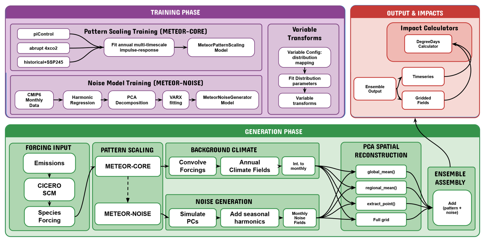
Figure 1 METEOR system workflow integrating pattern scaling, internal variability, and impacts assessment. Pattern scaling trains multi-timescale response patterns from CMIP6 annual data to predict forced climate response from emissions scenarios (purple box). Noise model training learns the structure of internal variability from CMIP6 monthly data, capturing seasonal cycles, spatial patterns (PCA), and temporal dynamics (VARX). Ensemble generation (green) combines the METEOR-predicted forced response with stochastic noise to produce large ensembles. Impacts module (red) calculates sector-relevant metrics such as heating degree days (HDD) and cooling degree days (CDD) from ensemble distributions, enabling uncertainty quantification for climate risk assessment.

3 Training: Learning the Structure of Variability

3.1 Preparing the Data

Training begins with monthly climate data from CMIP6, where by default we concatenate a model's historical simulation (1850–2014) with a mid-range future scenario SSP2-4.5 (2015–2100) (O'Neill et al., 2016), creating a continuous record of approximately 250 years from a single ensemble member. This extended record is used to characterize the statistical structure of internal variability (the dominant spatial patterns, persistence timescales, and teleconnections), though it represents just one realization of the climate trajectory (this keeps training data needs to a minimum and is practically found to allow defensible noise emulation, though future versions are expected to explore ensemble assimilation for noise training).

The global mean temperature (GMT) dependent seasonal model separates forced seasonality changes from internal variability, while PCA and VARX learn the structure of the residual fluctuations. We also subtract a pre-industrial baseline from the GMT using a pre-industrial control experiment, ensuring consistency with METEOR's pattern scaling framework. Global mean temperature is computed from this data as an area-weighted spatial average:

$$\begin{array}{}\text{(3)}& T_{\text{glob}}\left(t\right)={\displaystyle \frac{{\sum }_{i=\mathrm{1}}^s{w}_i\cdot X_i\left(t\right)}{{\sum }_{i=\mathrm{1}}^s{w}_i}},\end{array}$$

where w_i=cos (lat_i) are area weights for pixel i, with a total of s pixels. This global mean is then smoothed with a 5-year (60-month) running mean to remove high-frequency variability that would complicate seasonal cycle fitting while preserving the multi-decadal warming trend and any interannual to decadal variations that might modulate seasonality. This choice is not critical: refitting the noise model with 3- and 10-year windows changes the seasonal R² by less than 0.6 percentage points and the total variance explained by less than 0.1 percentage points (Fig. S17 in the Supplement).

3.2 Modeling the Seasonal Cycle

The seasonal cycle can evolve as climate changes (“Harmonic Regression” in Fig. 1). For instance, sea ice loss causes Arctic regions to warm much faster in winter than summer, fundamentally altering their seasonal cycle (Sejas and Taylor, 2023). To capture such effects, we need a seasonal model that responds to warming.

The model described below applies to both temperature and precipitation, and in principle to any other supported variable; variable-specific distributional treatment is discussed later. Harmonic representations of the seasonal cycle are well established in monthly-resolution climate emulation (Nath et al., 2022; Schöngart et al., 2024); the formulation here extends this by allowing the amplitude and phase of the harmonics to modulate linearly with global mean temperature.

We construct nine time-varying features at each monthly time step, where T_glob(t) denotes the smoothed (5-year running mean) global mean temperature defined in Eq. (3):

$$\begin{array}{}\text{(4)}& {\mathit{X}}_{\text{harm}}\left(t\right)=\left[\begin{array}{c}{T}_{\text{glob}}\left(t\right)\\ \cos \left(\frac{\mathrm{2}\mathit{\pi }t}{\mathrm{12}}\right)\\ \sin \left(\frac{\mathrm{2}\mathit{\pi }t}{\mathrm{12}}\right)\\ \cos \left(\frac{\mathrm{4}\mathit{\pi }t}{\mathrm{12}}\right)\\ \sin \left(\frac{\mathrm{4}\mathit{\pi }t}{\mathrm{12}}\right)\\ T_{\text{glob}}\left(t\right)\cdot \cos \left(\frac{\mathrm{2}\mathit{\pi }t}{\mathrm{12}}\right)\\ T_{\text{glob}}\left(t\right)\cdot \sin \left(\frac{\mathrm{2}\mathit{\pi }t}{\mathrm{12}}\right)\\ T_{\text{glob}}\left(t\right)\cdot \cos \left(\frac{\mathrm{4}\mathit{\pi }t}{\mathrm{12}}\right)\\ T_{\text{glob}}\left(t\right)\cdot \sin \left(\frac{\mathrm{4}\mathit{\pi }t}{\mathrm{12}}\right)\end{array}\right].\end{array}$$

The first feature is the smoothed global temperature. The next four are standard harmonic functions representing annual and semi-annual cycles, which can reconstruct any seasonal pattern through their weighted combination. The final four features allow modulation with climate change, multiplying global temperature by the harmonic functions and allowing seasonal amplitude to grow or shrink with warming and seasonal phase to shift.

At each spatial location (x,y), we perform a linear regression with these nine features predicting the observed temperature or precipitation:

$$\begin{array}{}\text{(5)}& \begin{array}{rl}X\left(t,x,y\right)& ={\mathit{\beta }}_{\mathrm{0}}\left(x,y\right)+\sum _{j=\mathrm{1}}^{\mathrm{9}}{\mathit{\beta }}_j\left(x,y\right)\\ & \cdot {\mathit{X}}_{\text{harm},j}\left(t\right)+\mathit{ϵ}\left(t,x,y\right),\end{array}\end{array}$$

where β₀ is the intercept, β_j are the regression coefficients for predictor $j\in [\mathrm{1},\mathrm{9}]$, and ϵ represents the residual. This yields nine coefficients per location plus an intercept. The fitted values represent the expected seasonal pattern at each point in time, accounting for warming. The residuals (the difference between ESM training values and fitted values) are the anomalies:

$$\begin{array}{}\text{(6)}& \begin{array}{rl}A\left(t,x,y\right)& =\mathit{ϵ}\left(t,x,y\right)=X\left(t,x,y\right)\\ & -\left[{\mathit{\beta }}_{\mathrm{0}}\left(x,y\right)+\sum _{j=\mathrm{1}}^{\mathrm{9}}{\mathit{\beta }}_j\left(x,y\right)\cdot {\mathit{X}}_{\text{harm},j}\left(t\right)\right].\end{array}\end{array}$$

This approach is low-dimensional (nine parameters per location) yet flexible enough to capture spatial changes in seasonality. The regression is independent across locations, and the linearity assumption is reasonable for monthly mean data over the range of warming observed in typical scenarios.

3.3 Extracting Spatial Patterns

After removing the seasonal cycle, we're left with monthly anomalies at each grid point over the full timeseries (“PCA decomposition” in Fig. 1). These anomalies exhibit spatial structure associated with internal variability. Our goal is to identify these dominant spatial patterns and generalize them, allowing for seasonal influence, which we achieve using Principal Component Analysis (PCA) and Vector AutoRegression with eXogenous variables (VARX).

We reshape our anomaly data into a matrix ${\mathbf{A}}_{\text{flat}}\in {\mathbb{R}}^{T\times S}$, where T is the number of monthly time steps and S is the number of spatial locations. PCA then decomposes this matrix as:

$$\begin{array}{}\text{(7)}& {\mathbf{A}}_{\text{flat}}=\mathit{Z}{\mathbf{E}}^T+\mathit{\mu },\end{array}$$

where Z contains the PC timeseries, E contains the EOF spatial patterns, and μ is the spatial mean (approximately zero after removing the seasonal cycle). The first PC and EOF capture the most variance, the second pair captures the most remaining variance orthogonal to the first, and so on. By default, we retain 40 PCs for both temperature and precipitation. For surface temperature, the seasonal model captures approximately 91 % of total variance, and the 40 PCs explain 75 %–80 % of the remaining anomaly variance, yielding a combined total of approximately 98 % of variance explained. Precipitation exhibits greater stochastic variability: the seasonal model explains approximately 32 % of variance, with PCs capturing 29 %–45 % of anomaly variance, for a combined total of 51 %–64 % (see Table S1)

PCA representation of the anomalies has several advantages. First, it achieves massive dimensionality reduction: instead of modeling 10 000+ grid points, we model 40 timeseries. Second, the spatial orthogonality simplifies subsequent statistical modeling by ensuring that each PC can be modeled independently without concerns about spatial multicollinearity (predictors so strongly correlated with one another that a regression cannot cleanly separate their effects).

An alternative to this time-domain approach is a frequency-domain decomposition such as Multi-Taper Method Singular Value Decomposition (MTM-SVD) (Mann and Park, 1994), which identifies spatiotemporal modes across a spectrum of frequencies and naturally accommodates non-stationary spectral characteristics. Our primary requirement here is generative rather than diagnostic: the PCA-VARX combination supports forward simulation of pattern amplitudes with global mean temperature entering as an exogenous predictor, whereas frequency-domain modes require an additional resynthesis step to construct ensembles under an arbitrary temperature trajectory. MTM-SVD nonetheless offers a useful independent diagnostic of the frequency content captured by the emulator, and a frequency-domain comparison remains a natural direction for future work.

3.4 Modeling Monthly Temporal Dynamics

We now have 40 timeseries of PC amplitudes spanning several centuries of simulated climate (“VARX fitting” in Fig. 1). How do we characterize their temporal behavior? We need a model that captures three phenomena: persistence of anomalies, statistical dependencies between modes (which can, in principle, reflect physical teleconnections such as tropical–extratropical coupling), and modulation by external factors (global warming might affect variability). VARX (Hamilton, 2020; Sims, 1980) is well-suited for this task. This approach models each month's PC value as a linear combination of all PCs in the previous two months, allowing for external variables and random terms:

$$\begin{array}{}\text{(8)}& \mathit{Z}\left(t\right)=\mathit{c}+{\mathbf{A}}_{\mathrm{1}}\mathit{Z}(t-\mathrm{1})+{\mathbf{A}}_{\mathrm{2}}\mathit{Z}(t-\mathrm{2})+\mathit{B}{\mathit{X}}_{\text{exog}}\left(t\right)+\mathit{\epsilon }\left(t\right),\end{array}$$

where Z(t) is the vector of 40 PC values at time t, c is a constant vector, A₁ and A₂ are 40 × 40 coefficient matrices for lags 1 and 2, B contains coefficients for exogenous variables, and $\mathit{\epsilon }\left(t\right)\sim \mathcal{N}(\mathbf{0},\mathbf{\Sigma })$ is the multivariate Gaussian innovation (the random shock drawn afresh each month) with covariance matrix Σ. The two-month lag allows the model to capture both immediate month-to-month persistence and longer memory.

The specific formulation we use includes three exogenous variables representing global temperature and a seasonal signal:

$$\begin{array}{}\text{(9)}& {\mathit{X}}_{\text{exog}}\left(t\right)=\left[\begin{array}{c}{T}_{\text{glob}}\left(t\right)\\ \cos (\mathrm{2}\mathit{\pi }t/\mathrm{12})\\ \sin (\mathrm{2}\mathit{\pi }t/\mathrm{12})\end{array}\right].\end{array}$$

A key feature of this framework is that the covariance matrix Σ of the innovation term ε(t) is learned directly from the ESM training data. This matrix encodes the ESM-specific structure of internal variability, including which modes co-vary and at what relative magnitudes. By sampling from this learned multivariate distribution, METEOR-NOISE generates ensembles whose internal variability is calibrated to the target ESM, rather than relying on generic or prescribed noise. This distinguishes METEOR from approaches that add independent noise at each grid point or use externally specified variability estimates.

Each PC's prediction then depends on lagged values of all 40 PCs and the global trend, not just itself. This allows the model to represent lagged statistical dependencies between PCs. Where such dependencies reflect physical teleconnections (for example, tropical Pacific SST anomalies preceding extratropical circulation responses by roughly one month), they are captured to the extent that these processes project onto the leading EOFs of the training data. The model thus has thousands of coefficients (40 PCs × 2 lags × 40 PCs plus exogenous terms), estimated efficiently using standard least-squares regression.

3.5 Storing the Trained Model

Once training completes, we have three sets of parameters: seasonal regression coefficients (9 values per grid point), PCA components (40 spatial patterns plus their variances), and VARX parameters (coefficient and covariance matrices). Trained models can be optionally saved using Python's pickle format. This allows rapid loading for ensemble generation without retraining.

4 Generation: Creating New Ensemble Members

Given a trained noise model and an annual-resolution climatological trajectory from METEOR-CORE, we can generate ensemble members that combine forced response with seasonality and internal variability (“Generation Phase” in Fig. 1).

4.1 Simulating Principal Components

The first step is generating synthetic PC timeseries. We initialize the first two months (corresponding to the lag-2 VARX model) with zero PC values, representing climatological conditions. This choice ensures that ensemble members start from a neutral state and quickly diverge based on independent sampling from the fitted Gaussian noise model, rather than inheriting specific patterns from the end of the training period. For each subsequent month, we:

1. Construct exogenous variables (for temperature): the new trajectory's global temperature for this month and the month-of-year encoded as sine and cosine. For precipitation (and for any other variable specified without override), the model will use a pure VAR model without exogenous variables for stability (further development will consider methods to incorporate exogenous forcing for non-temperature fields without sacrificing model stability).

2. Apply the VARX equation: compute a weighted sum of the previous two months' PC values across all modes, plus weighted exogenous variables (if applicable), plus the intercept. This gives the deterministic prediction.

3. Add random elements: draw from the fitted multivariate normal distribution with the learned covariance structure, and add to the deterministic prediction. This introduces stochasticity while preserving the inter-mode correlations observed in training.

4. Store the new PC values and advance to the next month.

This process is repeated for each ensemble member with independent random internal variability sampling. While ensemble members share the same VARX parameters and respond to the same temperature trajectory, their different random initializations cause them to diverge, exploring different realizations of internal variability.

For computational efficiency, all random innovations are pre-generated in a single batched multivariate normal draw before the time loop begins. This eliminates the overhead of thousands of separate random number generations and enables efficient vectorized operations, reducing generation time for large ensembles from minutes to seconds.

4.2 Reconstructing Spatial Fields

From simulated PCs, we reconstruct spatial climate fields in three steps. First, we compute the seasonal cycle for the new temperature trajectory. Using the nine harmonic features constructed from the new trajectory's global temperature and month-of-year, we multiply by the fitted seasonal coefficients at each location. This gives the expected seasonal pattern accounting for warming.

Second, we convert the simulated PCs back to spatial anomalies. This is the inverse of the PCA transformation:

$$\begin{array}{}\text{(10)}& A(t,x,y)=\sum _{k=\mathrm{1}}^{\mathrm{40}}{Z}_k\left(t\right)\cdot E_k(x,y),\end{array}$$

where Z_k(t) is the kth simulated PC at time t and E_k(x,y) is the kth learned EOF pattern at location (x,y). This reconstruction exhibits the same spatial covariance structure as the training data. Finally, we combine the seasonal cycle and spatial anomalies to get the complete field.

4.3 Integration with METEOR-CORE

For integration with METEOR-CORE (“Background climate” and “Noise Generation” in Fig. 1), we generate noise-only fields that exclude the forced warming component. The noise field at each location and time is:

$$\begin{array}{}\text{(11)}& \begin{array}{rl}N(t,x,y)& =\sum _{j=\mathrm{2}}^{\mathrm{9}}{\mathit{\beta }}_j(x,y)\cdot {\mathit{X}}_{\text{harm},j}\left(t\right)\\ & +\sum _{k=\mathrm{1}}^{\mathrm{40}}{Z}_k\left(t\right)\cdot E_k(x,y),\end{array}\end{array}$$

where we omit the intercept β₀ and the direct temperature term β₁T_glob(t), keeping only the harmonic terms (including the temperature-modulated harmonics) plus the stochastic anomalies. The forced warming signal is provided by the METEOR-CORE pattern scaling model.

METEOR-CORE produces annual mean predictions ${\stackrel{\mathrm{‾}}{X}}_{\text{METEOR}}(t_{\mathrm{a}},x,y)$ where $t_{\mathrm{a}}=\lfloor (t-\mathrm{1})/\mathrm{12}\rfloor +\mathrm{1}$ converts monthly time index t to year index t_a. To combine with monthly noise, we simply repeat each annual value for 12 months. The final ensemble member is the sum:

$$\begin{array}{}\text{(12)}& X_{\text{ensemble}}^{\left(m\right)}(t,x,y)={\stackrel{\mathrm{‾}}{X}}_{\text{METEOR}}(t_{\mathrm{a}},x,y)+N^{\left(m\right)}(t,x,y),\end{array}$$

where superscript (m) denotes ensemble member m.

This additive combination assumes forced response and internal variability are independent. The forced response provides the long-term trend and multi-decadal evolution, while the noise adds higher temporal fluctuations around that trend. This framework also lends itself to a forced scaling of the global warming signal to fit or predict to some distribution of global mean annual temperatures. We describe this further in Sect. 6.1.2.

4.4 Efficient Regional Calculations

A practical feature of the PC-based approach is that we can compute regional or global means without reconstructing full spatial fields. For any region ℛ, we pre-compute the area-weighted regional mean of each EOF pattern:

$$\begin{array}{}\text{(13)}& {\stackrel{\mathrm{‾}}{E}}_k^{\mathcal{R}}={\displaystyle \frac{{\sum }_{(x,y)\in \mathcal{R}}w\left(x\right)\cdot E_k(x,y)}{{\sum }_{(x,y)\in \mathcal{R}}w\left(x\right)}},\end{array}$$

where w(x)=cos (lat(x)) are latitude-based area weights as in Eq. (3). Then the regional mean anomaly at any time is:

$$\begin{array}{}\text{(14)}& {\stackrel{\mathrm{‾}}{A}}^{\mathcal{R}}\left(t\right)=\sum _{k=\mathrm{1}}^{\mathrm{40}}{Z}_k\left(t\right)\cdot {\stackrel{\mathrm{‾}}{E}}_k^{\mathcal{R}}.\end{array}$$

This matters for computational efficiency. If we want 100 ensemble members of global mean temperature over 350 years (42 000 monthly values per member), we can compute this directly from the 40 PCs without ever calculating the full spatial fields. This vastly reduces memory requirements and enables very large ensembles for either regions or point-site estimates.

4.5 Variable-Specific Processing

Different climate variables require distinct statistical treatments. Temperature anomalies are approximately Gaussian-distributed and can be processed directly using the PCA-VARX framework described above. However, precipitation presents additional challenges: it is bounded below by zero, exhibits strong positive skewness, and has fundamentally different statistical properties than temperature.

METEORv1.6 addresses this through a variable-specific transformation framework. For precipitation, the noise model output (which is approximately Gaussian) is transformed by default via quantile mapping to a gamma distribution:

$$\begin{array}{}\text{(15)}& P_{\text{transformed}}=F_{\mathrm{\Gamma }}^{-\mathrm{1}}\left(\mathrm{\Phi }\left({\displaystyle \frac{P_{\text{noise}}-\mathit{\mu }}{\mathit{\sigma }}}\right);k,\mathit{\theta }\right),\end{array}$$

where Φ is the standard normal CDF, $F_{\mathrm{\Gamma }}^{-\mathrm{1}}$ is the inverse gamma CDF, and (k,θ) are the shape and scale parameters fitted to the target ESM's precipitation distribution using maximum likelihood estimation. When fitting fails (e.g., at gridpoints with fewer than two positive samples), the code falls back to a canonical setting equivalent to method-of-moments estimation: $k={\mathit{\mu }}^{\mathrm{2}}/{\mathit{\sigma }}^{\mathrm{2}}$ and $\mathit{\theta }={\mathit{\sigma }}^{\mathrm{2}}/\mathit{\mu }$. In practice this fallback path does not fire on the NorESM2-MM SSP2-4.5 training grid used in this paper: every gridpoint retains at least 1021 of 1032 valid monthly samples, and the maximum-likelihood fit converges everywhere (Fig. S19). The quantile values are clipped to(10⁻¹⁰, 1–10⁻¹⁰) to ensure numerical stability at distribution tails.

Precipitation is processed as absolute values rather than anomalies. The core pattern scaling model provides the forced response, and the noise model adds realistic monthly variability, with the gamma transform ensuring the non-negativity constraint and preserving the characteristic right-skewed distribution observed in ESM output.

For temperature, anomalies are computed relative to a pre-industrial baseline derived from the pre-industrial control (piControl) experiment. The global mean piControl temperature is subtracted from the training data before computing the smoothed temperature trajectory used for seasonal cycle modulation.

The framework is extensible through a transform registry, which maps variable names to configuration objects specifying the transform type and fitting/application functions. For regional and global mean calculations, supported transforms include gamma, Weibull, log-normal, and generalized gamma distributions, as well as empirical (non-parametric) quantile mapping. For fully gridded fields, currently only the gamma distribution is implemented.

5 Computational Performance

The methodology is designed for computational efficiency at both training and generation stages.

Training a noise model for a typical CMIP6 resolution (approximately 96 × 144 spatial grid, 3000 monthly time steps, 40 PCs) takes 30–60 s on a standard laptop. The process is dominated by Principal Component Analysis, which scales roughly quadratically with spatial resolution. Models at higher resolution or with longer training periods remain tractable in several minutes at most for high-resolution ESMs.

Generation speed varies by output type. For regional or global mean timeseries (e.g., global mean temperature or precipitation for a continent), producing 100 ensemble members covering 350 years at monthly resolution takes approximately 90 s on a standard laptop. For point-based extraction (e.g., a single city), the same computation takes roughly 10 s for 100 members, enabling ensembles of 1000+ members in under 2 min. Reconstructing full spatial fields is more expensive, scaling with grid resolution. This performance comes from batch random number generation and vectorized linear algebra operations that avoid explicit loops over ensemble members.

Memory requirements depend on the use case. Full spatial fields for large ensembles can quickly exceed available memory on a conventional laptop, but storing only PCs reduces requirements by 2–3 orders of magnitude. For most applications, a hybrid approach works well: store PCs for all members, then reconstruct variability for large ensembles in regions of interest as needed.

METEORv1.6 provides a unified high-level interface that manages training, caching, and ensemble generation through a single entry point. This interface handles automatic caching of intermediate results, variable-specific transforms, and flexible output aggregation (global means, IPCC Sixth Assessment Report (AR6) regional means (IPCC, 2021), or point-based extraction), enabling users to generate probabilistic climate projections with minimal configuration.

6 Impact Assessment Framework

6.1 Modular Calculator Architecture

The impact assessment framework provides a standardized interface for converting climate projections into sectoral impact metrics while preserving METEOR's uncertainty characteristics and ensemble capabilities. The system is built around an extensible ImpactCalculator base class that defines common methods for climate data preprocessing and validation with METEOR-specific metadata, impact metric calculation with configurable parameters, ensemble processing and uncertainty quantification, and statistical analysis and results summarization consistent with METEOR's multi-forcing framework.

This modular design enables rapid development of sector-specific impact calculators while maintaining consistency in uncertainty treatment and ensemble analysis across different applications. The framework automatically propagates uncertainty from METEOR's climate projections through to impact metrics, enabling probabilistic impact assessments that account for both climate model uncertainty and natural variability.

6.1.1 Degree Days Implementation

The initial implementation includes a degree days calculator for energy sector applications, adapting them for METEOR's monthly climate outputs. Heating degree days (HDD) and cooling degree days (CDD) are conventionally defined as:

$$\begin{array}{}\text{(16)}& {\displaystyle }\text{HDD}& {\displaystyle }=\sum _{\mathrm{d}}max(T_{\text{base}}-T_{\mathrm{d}},\mathrm{0})\text{(17)}& {\displaystyle }\text{CDD}& {\displaystyle }=\sum _{\mathrm{d}}max(T_{\mathrm{d}}-T_{\text{base}},\mathrm{0})\end{array}$$

where T_d represents daily outdoor temperature and T_base is the base temperature threshold (typically 15–18 °C), the temperature above (below) which a building doesn't need heating (air conditioning). Since METEOR produces monthly mean temperatures rather than daily values, the implementation uses the statistical method of Isaac and Van Vuuren (2009), which estimates degree days from monthly means by assuming daily temperatures follow a normal distribution. The method uses an empirical parameterization of intra-monthly temperature variability based on Erbs et al. (1982):

$$\begin{array}{}\text{(18)}& {\mathit{\sigma }}_{\mathrm{m}}=c_{\mathrm{1}}-c_{\mathrm{2}}{T}_{\mathrm{m}}+c_{\mathrm{3}}{\mathit{\sigma }}_y,\end{array}$$

where σ_m is the estimated standard deviation of daily temperatures within month m, T_m is the monthly mean temperature, σ_y is the annual standard deviation of monthly means, and $(c_{\mathrm{1}},c_{\mathrm{2}},c_{\mathrm{3}})=(\mathrm{1.45},\mathrm{0.29},\mathrm{0.664})$ are default empirical coefficients derived from observational data, assumed constant under climate change (a simplification that may introduce bias under substantially altered variability regimes). The degree days are then computed analytically from this assumed distribution, avoiding the need for daily temperature data while still accounting for within-month variability.

6.1.2 Scaling results to a GMT timeseries

Traditional pattern scaling approaches such as MESMER (Beusch et al., 2020) and also more inventive approaches such as STITCHES (Tebaldi et al., 2022) employ global mean timeseries data, primarily global mean temperature (GMT), to scale their mean outputs. While METEOR inherently moves away from this approach to be able to model path- and forcer-dependent patterns, regional climate signals are strongly coupled to global mean temperature (Giani et al., 2025), and GMT-based scaling remains a useful approximation for many applications. This capability enables direct integration with multi-emulator comparison frameworks such as FastMIP (Seneviratne et al., 2024), where emulators are evaluated against a common GMT trajectory, and facilitates comparison with other pattern scaling approaches that use GMT as their primary scaling variable. It also allows METEOR projections to be conditioned on GMT trajectories from different ESMs or simple climate models, extending the framework's applicability beyond the training ESM.

METEOR v1.6 therefore includes an option to include a GMT timeseries as input to the emulation generation, in addition to the gridded ESM training data. This GMT information is then integrated into the generation of emulated qualities described above in the following way: In the integration with METEOR-CORE described in Sect. 4.3, annual patterns are first generated using METEOR-CORE. The associated GMT timeseries is produced alongside those patterns even if temperature is not itself a target variable. These annual patterns are scaled by the ratio of the provided global mean temperature timeseries to the METEOR-CORE emulated global mean timeseries. The resulting scaled annual patterns are then what is used in the ensemble generation of Eq. (12) as if they were the emulation result of METEOR-CORE. Illustrative examples of this scaling approach are shown in Figs. S13 and S14.

7 Results

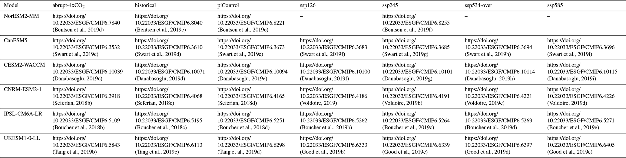
We validate METEORv1.6 in two stages. First, we demonstrate in-sample performance by training the emulator on SSP2-4.5 output from NorESM2-MM and evaluating the fidelity of the resulting ensemble against the training data. Second, we assess out-of-sample generalization by training on SSP2-4.5 across five CMIP6 models (see Table 1 and code availability section for model listing and links to their dataset URLs) and evaluating predictions for scenarios not seen during training (SSP1-2.6 – a high mitigation scenario, SSP5-8.5 – an exceptionally high emissions scenario, and SSP5-3.4-Overshoot – a strong overshoot scenario) (O'Neill et al., 2016). In each case, we present an illustrative example in the main text; a more comprehensive assessment across all models and spatial scales is provided in the Supplement.

(Bentsen et al., 2019d)(Bentsen et al., 2019c)(Bentsen et al., 2019e)(Bentsen et al., 2019f)(Swart et al., 2019c)(Swart et al., 2019d)(Swart et al., 2019e)(Swart et al., 2019f)(Swart et al., 2019g)(Swart et al., 2019h)(Swart et al., 2019i)(Danabasoglu, 2019c)(Danabasoglu, 2019d)(Danabasoglu, 2019e)(Danabasoglu, 2019f)(Danabasoglu, 2019g)(Danabasoglu, 2019h)(Danabasoglu, 2019i)(Seferian, 2018b)(Seferian, 2018c)(Seferian, 2018d)(Voldoire, 2019)(Voldoire, 2019b)(Voldoire, 2019c)(Voldoire, 2019d)(Boucher et al., 2018b)(Boucher et al., 2018c)(Boucher et al., 2018d)(Boucher et al., 2019b)(Boucher et al., 2019c)(Boucher et al., 2019d)(Boucher et al., 2019e)(Tang et al., 2019b)(Tang et al., 2019c)(Tang et al., 2019d)(Good et al., 2019b)(Good et al., 2019c)(Good et al., 2019d)(Good et al., 2019e)

Table 1 CMIP6 simulations used in this study. Table entries are references to the table DOI and a full detailed listing is found in the corresponding bibliography entry. NorESM2-MM is the in-sample training model and was not used for the out-of-sample scenario evaluation, so the additional scenarios are not required (denoted –).

7.1 In-Sample Validation

7.1.1 Distributional Fidelity

Figure 2 provides an overall illustration that the METEOR emulator produces climate distributions consistent with the source ESM. The figure shows METEOR ensemble projections (100 realizations) against NorESM2-MM output for the near-term period (2015–2035), demonstrating that the emulated distributions capture both the central tendency and spread of the year-to-year variation in NorESM across multiple spatial scales (global, regional and point) and for both temperature and precipitation.

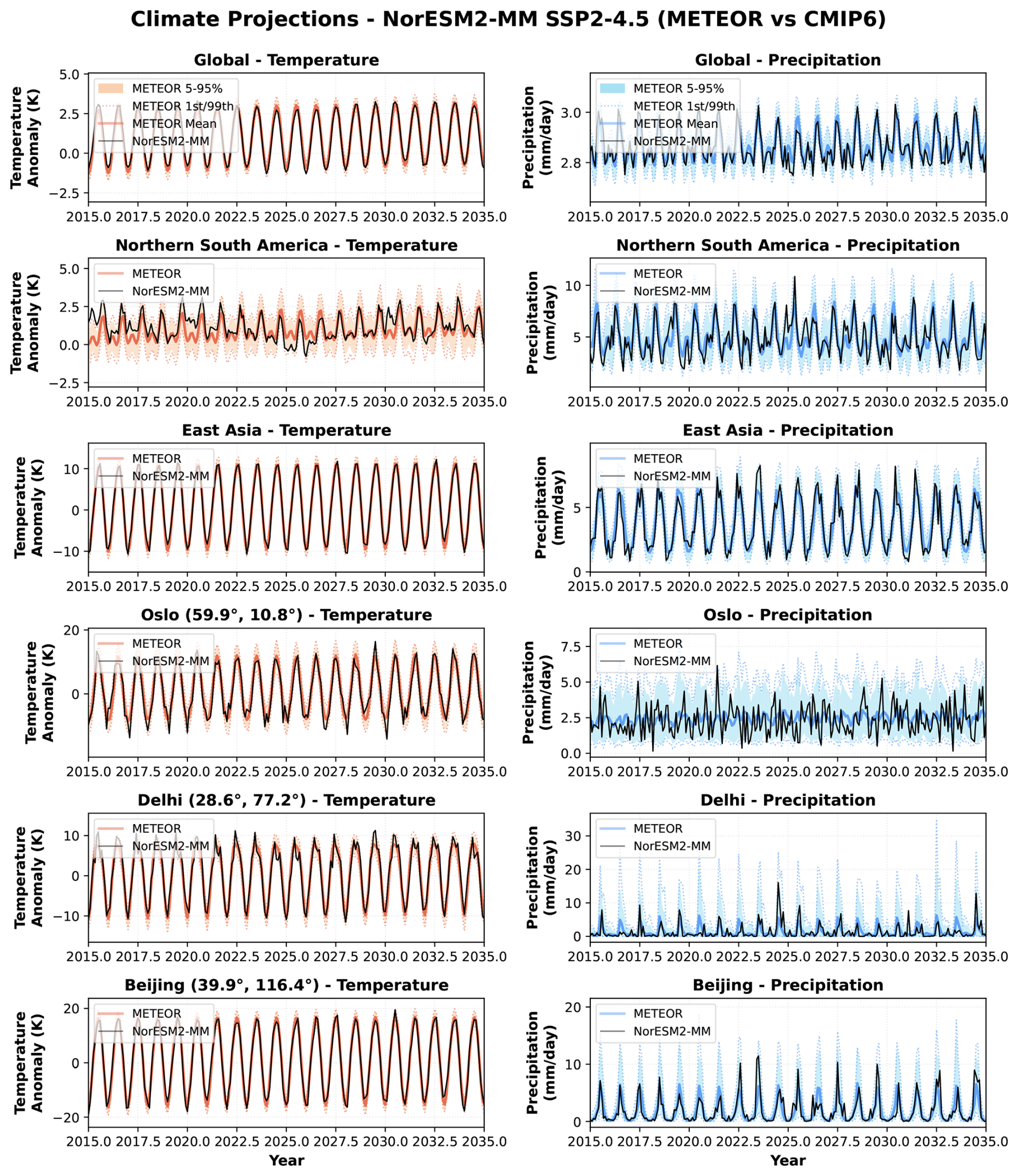
Figure 2 METEOR ensemble projections (100 realizations) compared with NorESM2-MM SSP2-4.5 output for 2015–2035. The emulated distributions capture both the forced response (emulated by METEOR-CORE) and seasonal cycle/internal variability (emulated by METEOR-NOISE) of the source model across multiple spatial scales (global, regional and point).

7.1.2 Long-Term Climate Trends

Figure 3 extends the evaluation to the full scenario period (2000–2100), demonstrating that long-term climate trends are preserved by METEORv1.6 at regional scales. The multi-decadal warming trajectory and associated precipitation changes of the source simulation are well captured by the emulator, indicating that the pattern scaling foundation of METEOR-CORE combined with METEOR-NOISE qualitatively captures forced responses and variability over extended time horizons.

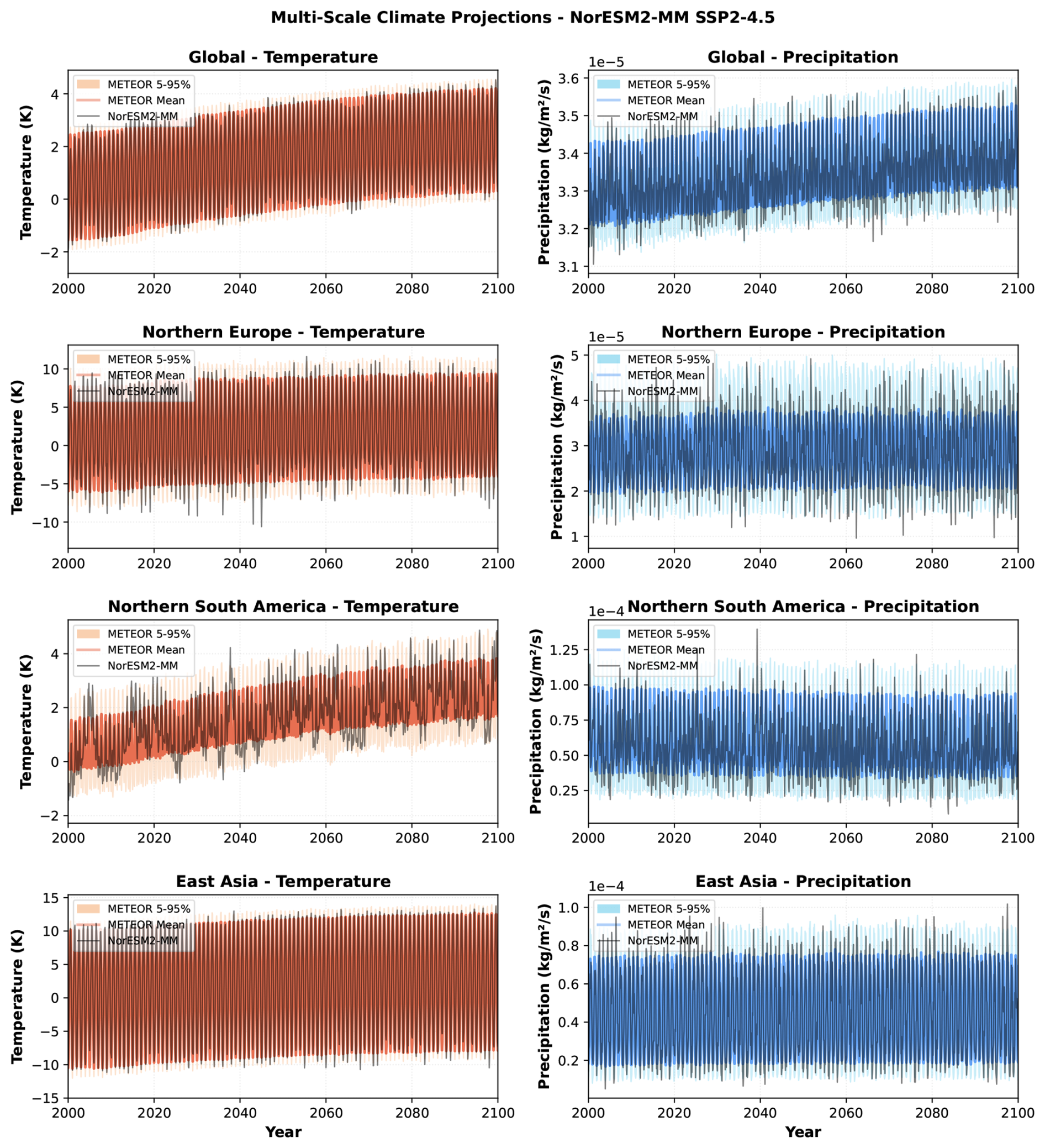
Figure 3 METEOR ensemble projections compared with NorESM2-MM SSP2-4.5 output for the extended period 2000–2100, showing that long-term regional climate trends are preserved by the emulator.

7.1.3 Seasonal Cycle and Distributional Shifts

A critical test of the monthly extension with METEOR-NOISE is its ability to reproduce evolving seasonal patterns and distributional characteristics. Figure 4 illustrates this at four contrasting point locations: Oslo, Delhi, Cairo and Beijing, capturing evident features from the source simulation in each case. In Delhi, the emulator captures the reduction in the seasonal temperature cycle under warming and the increasing variability in precipitation. In Oslo, similar preservation of increasing precipitation variability is evident. These results validate the temperature-dependent harmonic representation of the seasonal cycle described in Sect. 2, which allows both seasonal amplitude and phase to evolve with the background climate state.

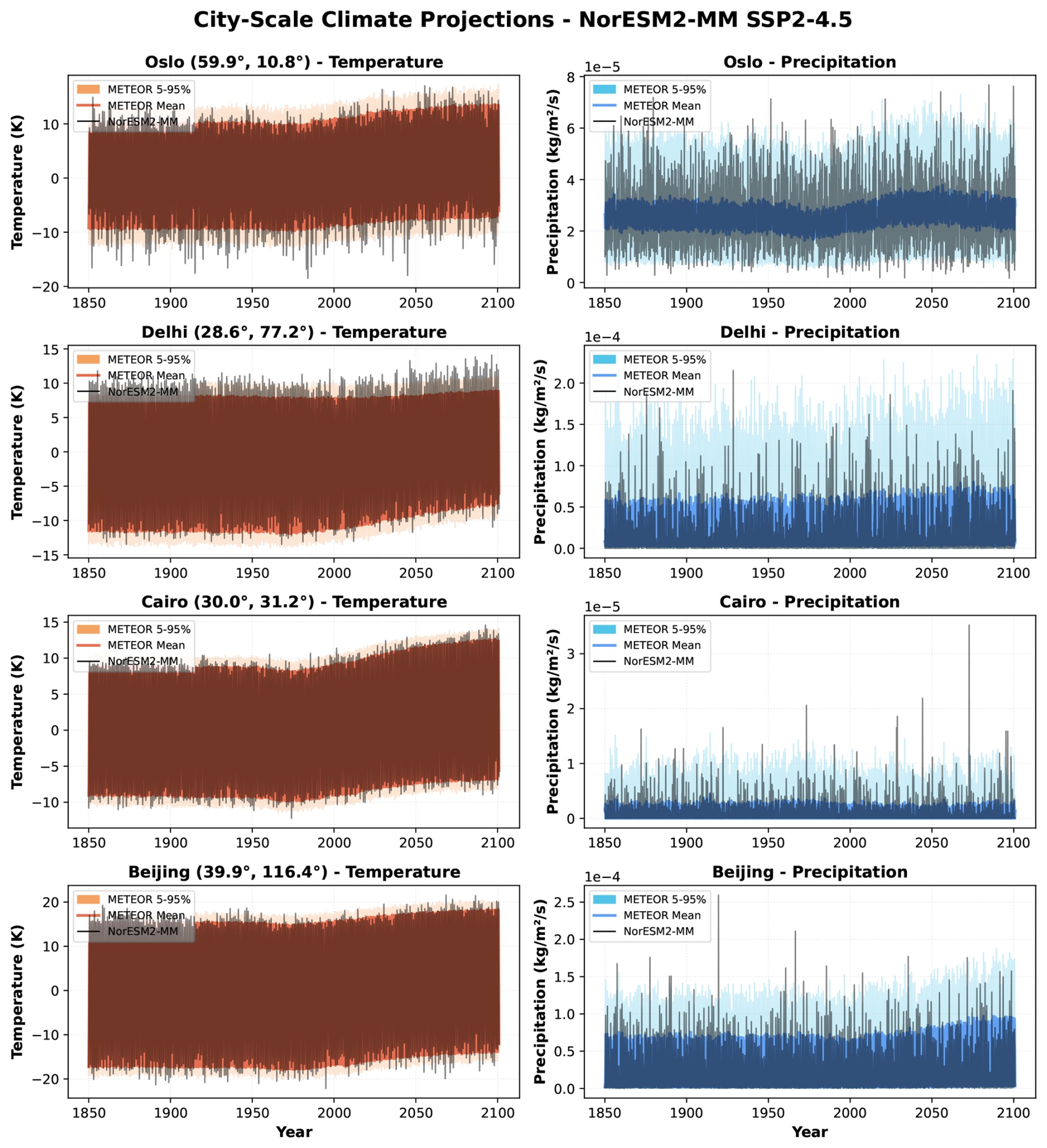
Figure 4 City-scale projections (1850–2100) for a number of cities, demonstrating that METEORv1.6 preserves distributional trends and seasonal cycle shifts.

7.1.4 Ensemble Adequacy

We assess ensemble adequacy using rank histograms, which objectively test whether the CMIP6 output is statistically indistinguishable from a random draw of the METEOR ensemble. For each time step, we compute the normalized rank of the CMIP6 value within the METEOR ensemble; a uniform rank distribution indicates that the ensemble adequately spans the observed variability. A flat histogram indicates that the source model is indistinguishable from the ensemble, a u-shaped histogram indicated that the ensemble is underdispersive (i.e. the source model tends to fall outside the emulated ensemble more often than would be expected from a perfect emulation), while clustering towards the center of the histogram would indicate overdispersion (that the emulated ensemble exhibits too much variance).

Figure 5 shows in-sample rank histograms for NorESM2-MM across multiple regions and for both variables. Temperature ranks are broadly uniform across most regions, indicating appropriate ensemble dispersion, though slight underdispersion is evident for some regions (North South America region, Delhi gridcell). For precipitation, ranks are generally well-calibrated, with some underdispersion apparent for Northern Europe and Beijing. These results indicate that the PCA-VARX framework captures the dominant modes of internal variability, though the Gaussian noise assumption may slightly underestimate the tails of the distribution in certain regions. Global projections for both temperature and precipitation are slightly underdispersive.

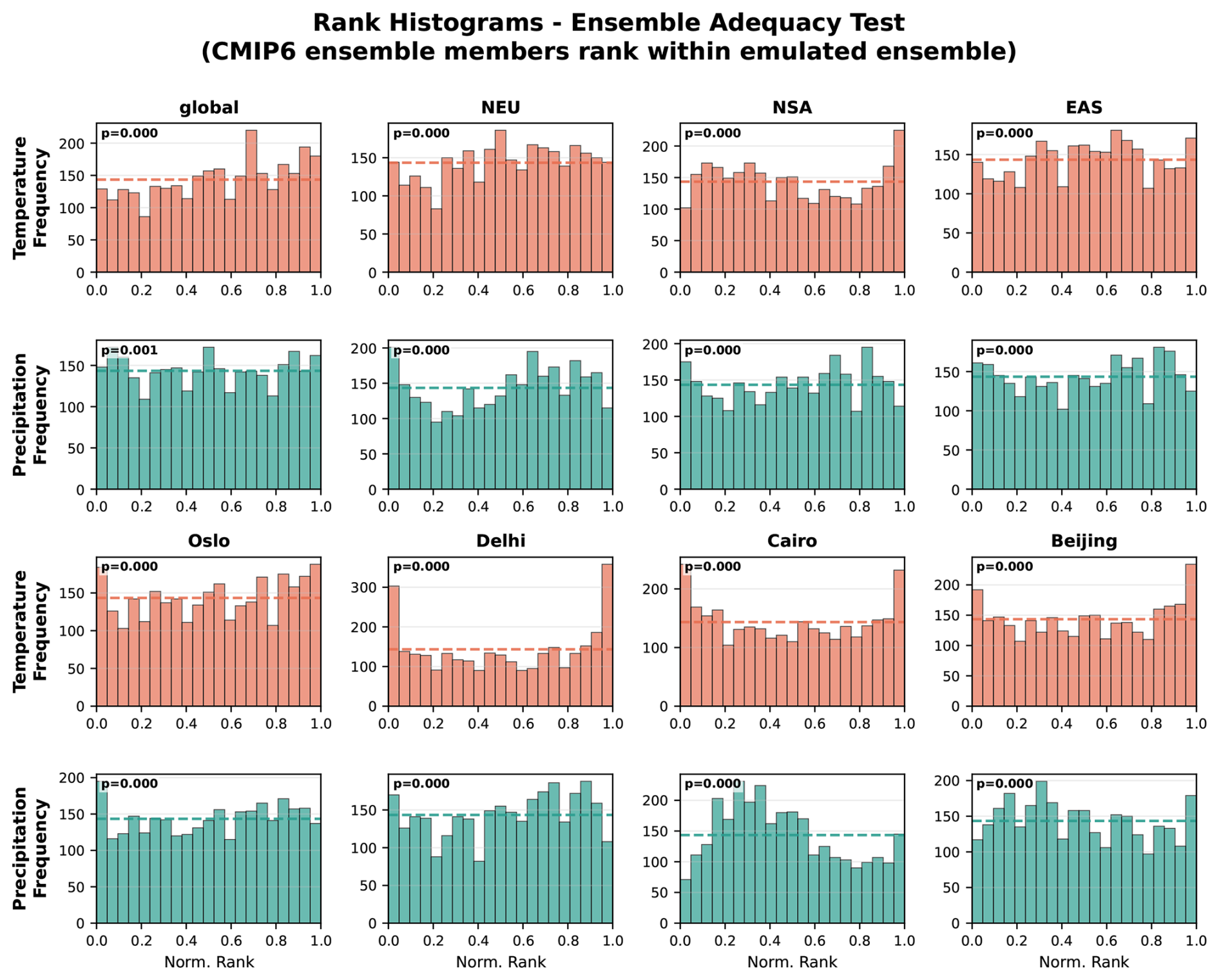
Figure 5 In-sample rank histograms for NorESM2-MM (SSP2-4.5) across multiple regions and variables. A uniform distribution (dashed line) indicates a perfectly representative ensemble. Each panel is annotated with the chi-squared uniformity p-value on the 21-bin count vector (df = 20); values shown in bold indicate p< 0.05, i.e. formal rejection of the uniformity null.

7.1.5 Impact Metrics: Degree Days

Figure 6 demonstrates the integrated impact assessment capabilities of METEORv1.6 through heating degree day (HDD) and cooling degree day (CDD) calculations. The emulator shows strong in-sample performance for these evolving impact metrics, capturing several notable features. In Beijing, the emulator reproduces the increase in HDD demands during the late 20th century associated with aerosol-driven regional cooling, demonstrating that METEOR's multi-forcer pattern scaling correctly propagates aerosol effects through to impact metrics at monthly resolution. In Oslo, cooling demands are essentially absent until the mid-21st century. This feature is faithfully preserved by METEOR, which correctly represents the threshold behavior despite never being explicitly trained on degree day targets. These results demonstrate end-to-end uncertainty propagation from climate projections through to sectoral impact metrics.

Here, the target is the Isaac and Van Vuuren (2009) algorithm applied directly to NorESM output. Future work will look into daily and subdaily temperature emulation using high temporal frequency output from NorESM to test this algorithm's performance, but this requires significant additional processing of high frequency output and is beyond the scope for this paper.

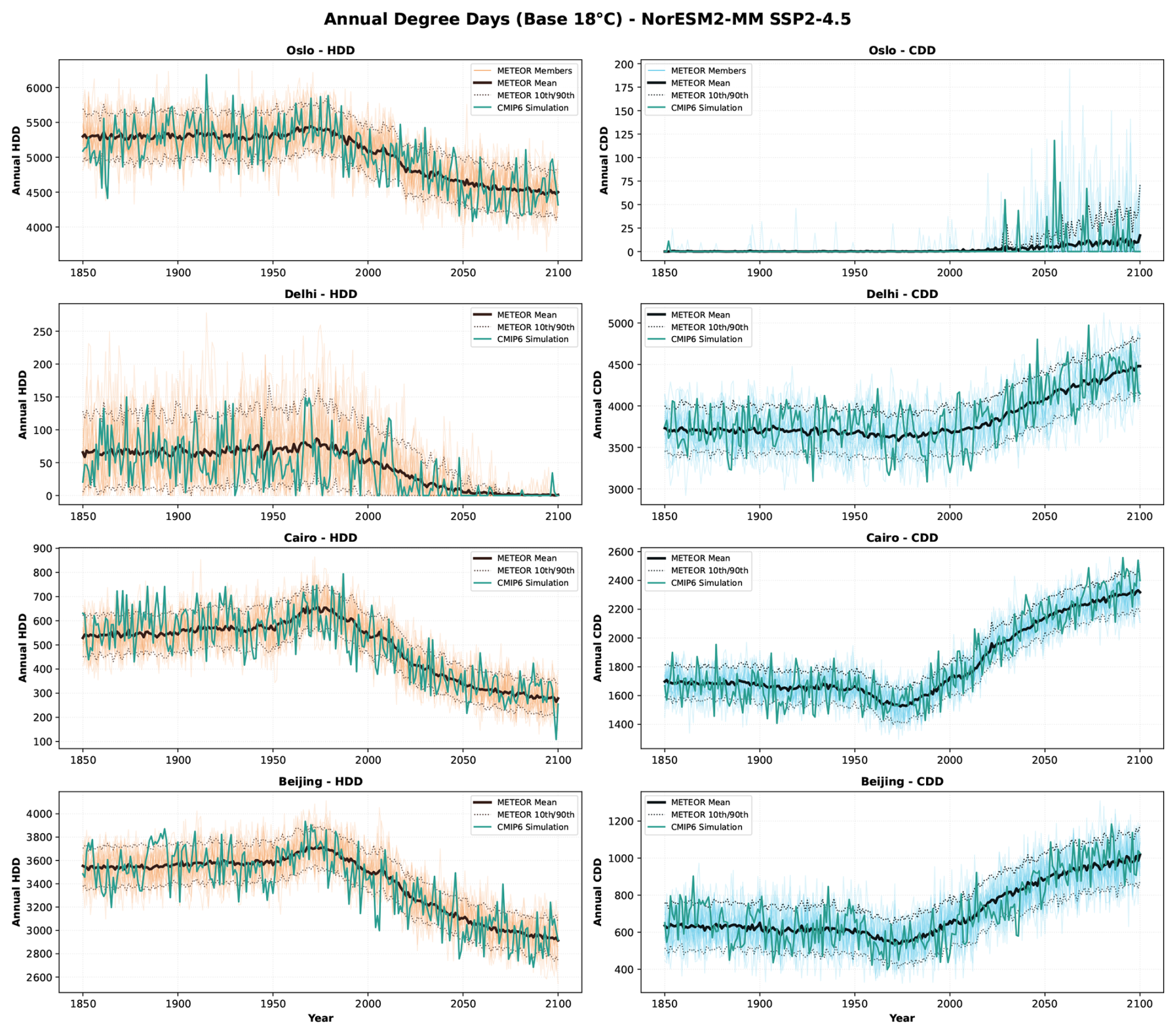
Figure 6 Heating degree days (HDD) and cooling degree days (CDD) for selected cities, comparing METEOR ensemble projections with NorESM2-MM. Notable features include the aerosol-related increase in HDD in Beijing during the late 20th century and the absence of cooling demands in Oslo until mid-21st century, both faithfully reproduced by the emulator.

7.2 Out-of-Sample Validation

To assess generalization beyond the training scenario, we train METEORv1.6 on SSP2-4.5 and evaluate predictions for SSP1-2.6, SSP5-8.5, and SSP5-3.4-Overshoot. Here, we demonstrate model performance for five models which performed simulations in CMIP6 for this entire set of scenarios: CanESM5, CESM2-WACCM, CNRM-ESM2-1, IPSL-CM6A-LR, and UKESM1-0-LL.

7.2.1 Multi-Scale Timeseries

In the main paper, we show CNRM-ESM2-1 as an out-of-sample example; equivalent results for all five models are provided in the Supplement. Figure 7 shows temperature anomaly projections across five spatial scales (global mean, East Asia, Northern Europe, Mumbai, and Oslo) for all four scenarios. The METEOR ensemble captures the CMIP6 climate signal across all spatial scales and scenarios. Both mean signals and variability characteristics are well captured in diverse out-of-sample scenarios, including under strong mitigation in SSP1-2.6 and for the overshoot scenario SSP5-3.4-OS, where CNRM-CM6's non-monotonic temperature trajectory is well reproduced. This highlights that METEOR-CORE's multi-timescale impulse response representation for scenarios, combined with the METEOR-NOISE model can represent the outcome of reversing forcing trends.

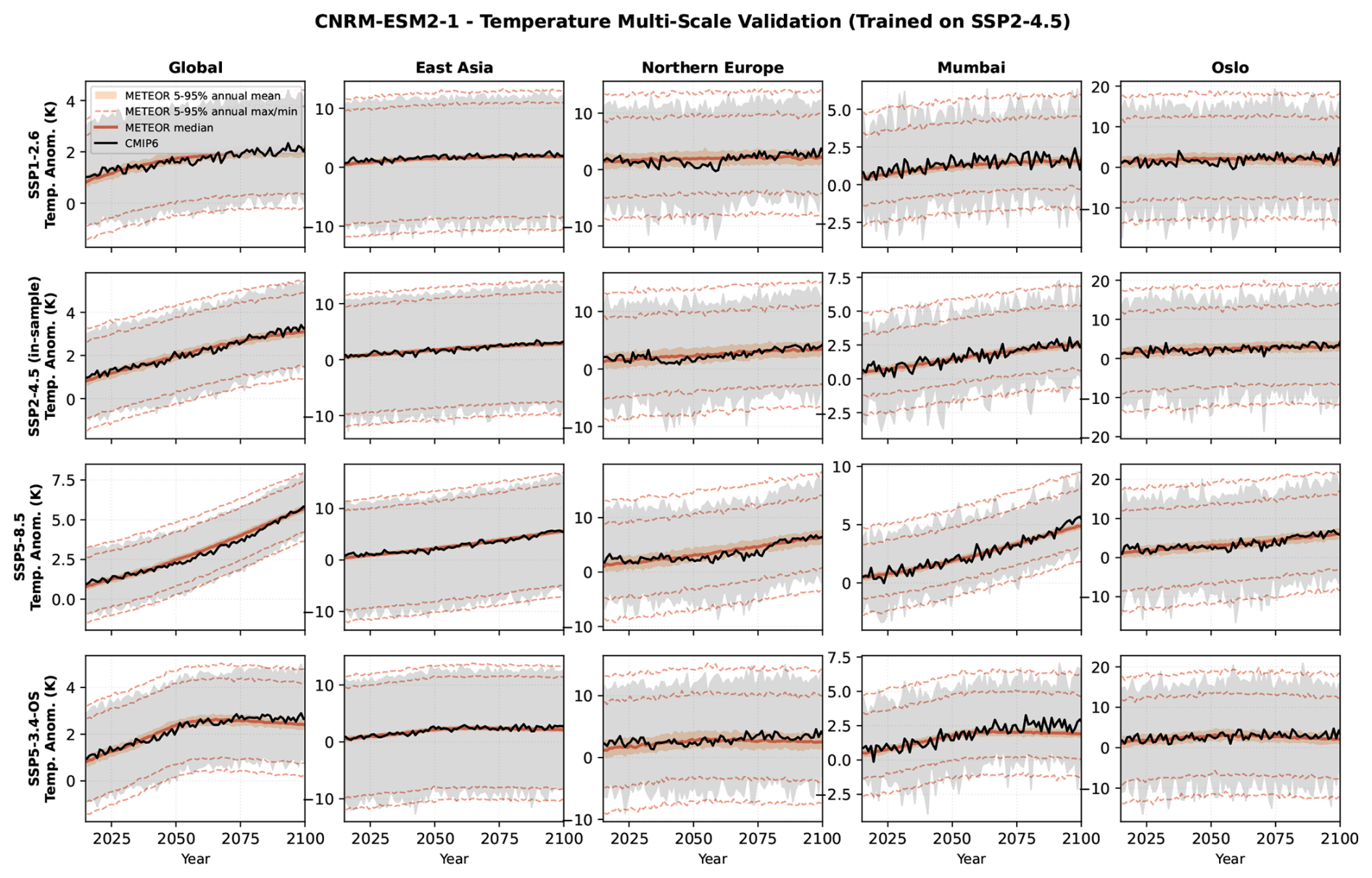
Figure 7 Out-of-sample temperature validation for CNRM-ESM2-1 trained on SSP2-4.5. Each row shows a validation scenario (SSP1-2.6, SSP2-4.5, SSP5-8.5, SSP5-3.4-OS); each column shows a spatial scale (global, East Asia, Northern Europe, Mumbai, Oslo). Orange shading: METEOR 5 %–95 % ensemble range of annual means. Orange dashed lines: 5 %–95 % range of annual maximum and minimum values. Orange solid line: ensemble median of annual means. Black line and grey shading: CMIP6 annual mean and monthly min/max envelope. Results for other models are shown in Figs. S1–S4.

Figure 8 shows the corresponding precipitation projections. The forced precipitation response is generally well captured, though precipitation changes under the high-emissions SSP5-8.5 are somewhat underestimated at some scales. This is consistent with the known challenge that precipitation responses can exhibit stronger nonlinearity with forcing magnitude than temperature responses, and that the pattern scaling relationship trained on a moderate forcing scenario (SSP2-4.5) may not fully extrapolate to the strongest forcing case.

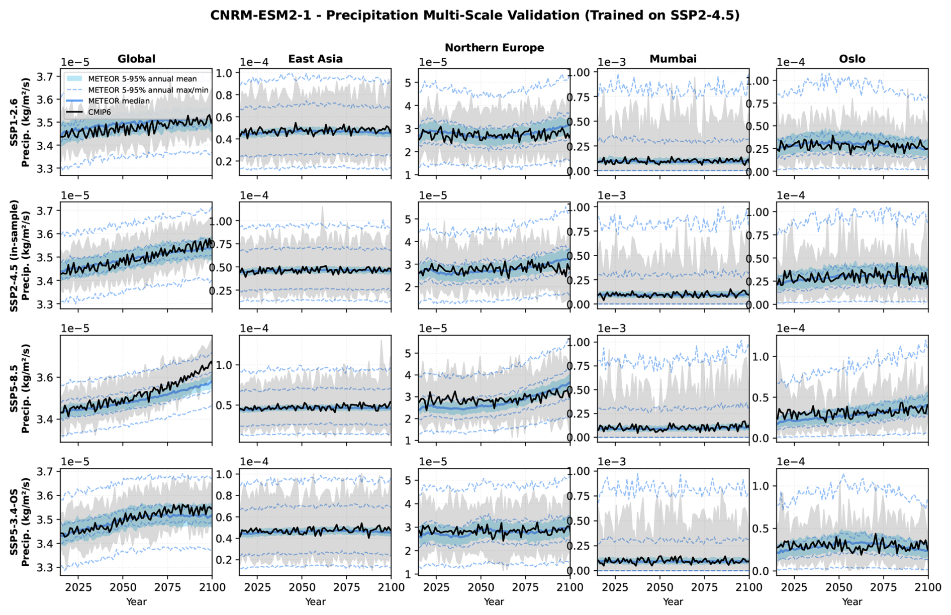
Figure 8 Out-of-sample precipitation validation for CNRM-ESM2-1 trained on SSP2-4.5. Layout and visual encoding as in Fig. 7: blue shading shows the 5 %–95 % range of annual means, dashed lines show the 5 %–95 % range of annual extrema, and the solid line shows the ensemble median. Precipitation changes are generally well captured, though SSP5-8.5 changes are somewhat underestimated. Results for other models are shown in Figs. S5–S8.

7.2.2 Out-of-Sample Ensemble Adequacy

Figure 9 shows rank histograms for an example gridcell (Oslo) across all four validation scenarios and five models, assessing whether the METEOR ensemble adequately spans the CMIP6 variability in out-of-sample conditions. Temperature distributions are well emulated for all scenarios, with rank histograms either uniform or slightly overdispersive across all models. Precipitation shows underdispersion to different degrees in different models – IPSL-CM6A-LR is well represented, for example but CanESM5 is notably underdispersive). Interestingly, global-scale precipitation rank histograms (Fig. S9) show more pronounced underdispersion than point-scale results, suggesting that the precipitation distributional transform may be less appropriate for large-scale spatial aggregations where individual grid-cell biases are averaged rather than cancelling. Coordinate transforms as a function of spatial scale are a development goal for future versions. Rank histograms for additional spatial scales are provided in the Supplement.

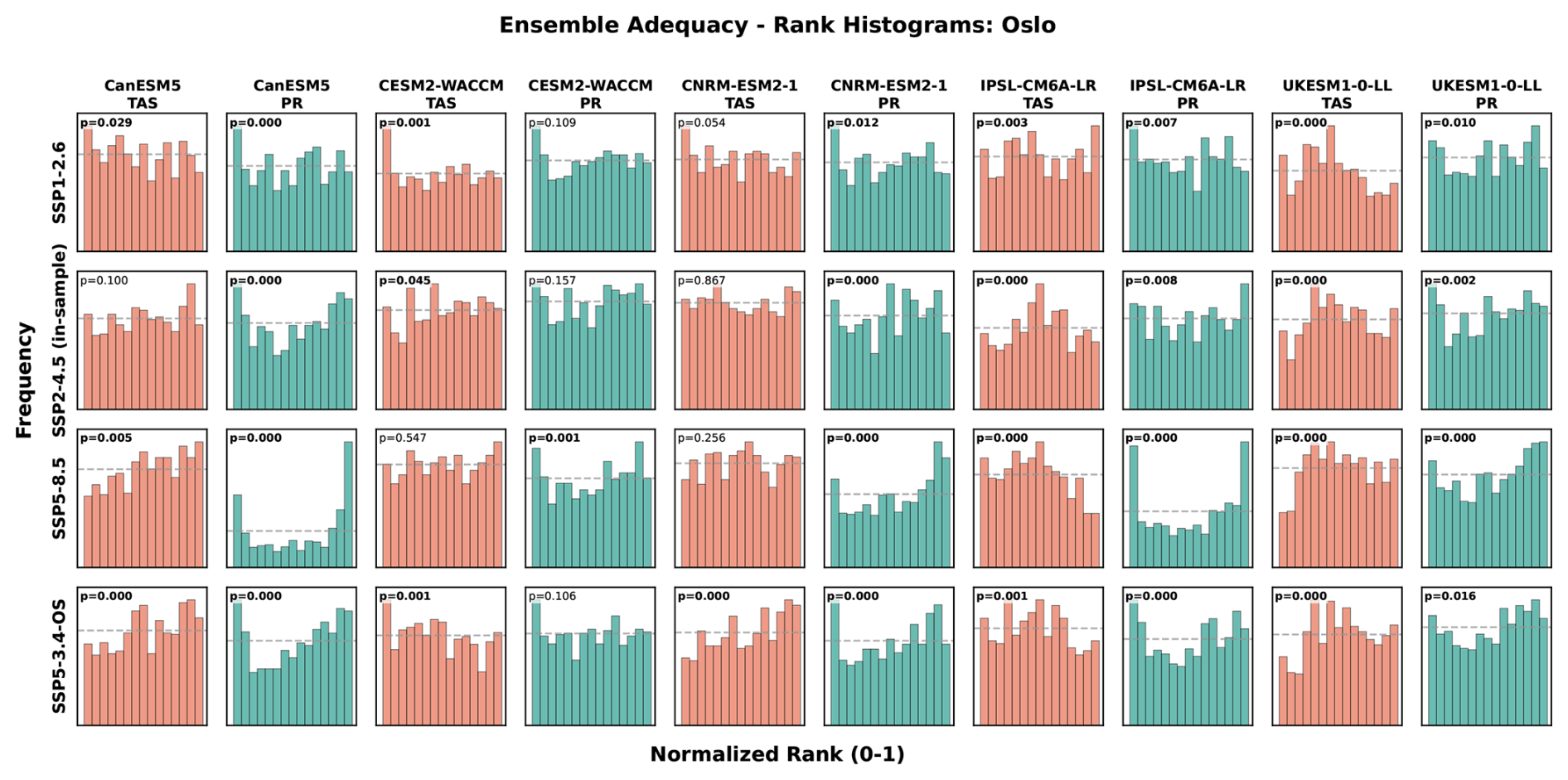
Figure 9 Out-of-sample rank histograms for Oslo across all scenarios and models. Each row shows a scenario; each pair of columns shows temperature and precipitation for one model. Temperature ranks are approximately uniform, indicating good ensemble calibration. Precipitation shows slight underdispersion. Each panel is annotated with the chi-squared uniformity p-value on the 15-bin count vector (df = 14); values shown in bold indicate p< 0.05. Rank histograms for other spatial scales are shown in Figs. S9–S12.

7.2.3 Quantitative Validation Metrics

For a stochastic emulator, the appropriate validation question is not whether individual ensemble members match the CMIP6 realization (they cannot, since stochastic sequences are inherently unpredictable) but whether the CMIP6 realization is statistically indistinguishable from an ensemble member. We assess this using skill ratios that compare member-CMIP6 metrics against member-member metrics. For both correlation and RMSE, we define the ratio such that values greater than 1 indicate poorer emulation:

$$\begin{array}{}\text{(19)}& \text{Correlation\hspace{0.17em}Skill\hspace{0.17em}Ratio}={\displaystyle \frac{\text{Member-Member\hspace{0.17em}correlation}}{\text{Member-CMIP6\hspace{0.17em}correlation}}}\end{array}$$

$$\begin{array}{}\text{(20)}& \text{RMSE\hspace{0.17em}Skill\hspace{0.17em}Ratio}={\displaystyle \frac{\text{Member-CMIP6\hspace{0.17em}RMSE}}{\text{Member-Member\hspace{0.17em}RMSE}}}\end{array}$$

If the emulator is well-calibrated, the CMIP6 output should be no more or less similar to ensemble members than members are to each other, yielding skill ratios near unity. For both metrics, ratios greater than 1 indicate poorer emulation: either systematic bias in the forced response (for RMSE) or lower-than-expected correlation (for correlation). Ratios below 1 indicate the ensemble may be underdispersive-members are too similar to each other, consistent with U-shaped rank histograms. This can be considered “hedging” results by underestimating variability with a simulation closer to the ensemble mean.

Figure 10 shows skill ratios across all spatial scales, models, and scenarios. Temperature skill ratios are consistently near 1.0 for both correlation (range 0.98–1.12) and RMSE (0.88–1.84), indicating that the emulator faithfully reproduces temperature variability characteristics across all scales with minimal systematic bias.

Precipitation skill varies more with scale. At global scales, precipitation correlation ratios are near unity (1.02–1.18) but RMSE ratios are elevated (1.4–7.0), suggesting pattern scaling does not fully capture the forced global precipitation response. At regional scales (East Asia, Northern Europe), precipitation correlation ratios remain near unity (1.02–1.43) with RMSE ratios of 1.1–1.8. At point scales, precipitation correlation ratios show greater variability (0.88–3.4 across Oslo and Mumbai), with Oslo showing the largest values, reflecting that point-scale precipitation correlation is dominated by stochastic variability where even small absolute differences produce large ratios. Mumbai shows ratios closer to unity, suggesting better distributional matching for monsoon-dominated precipitation.

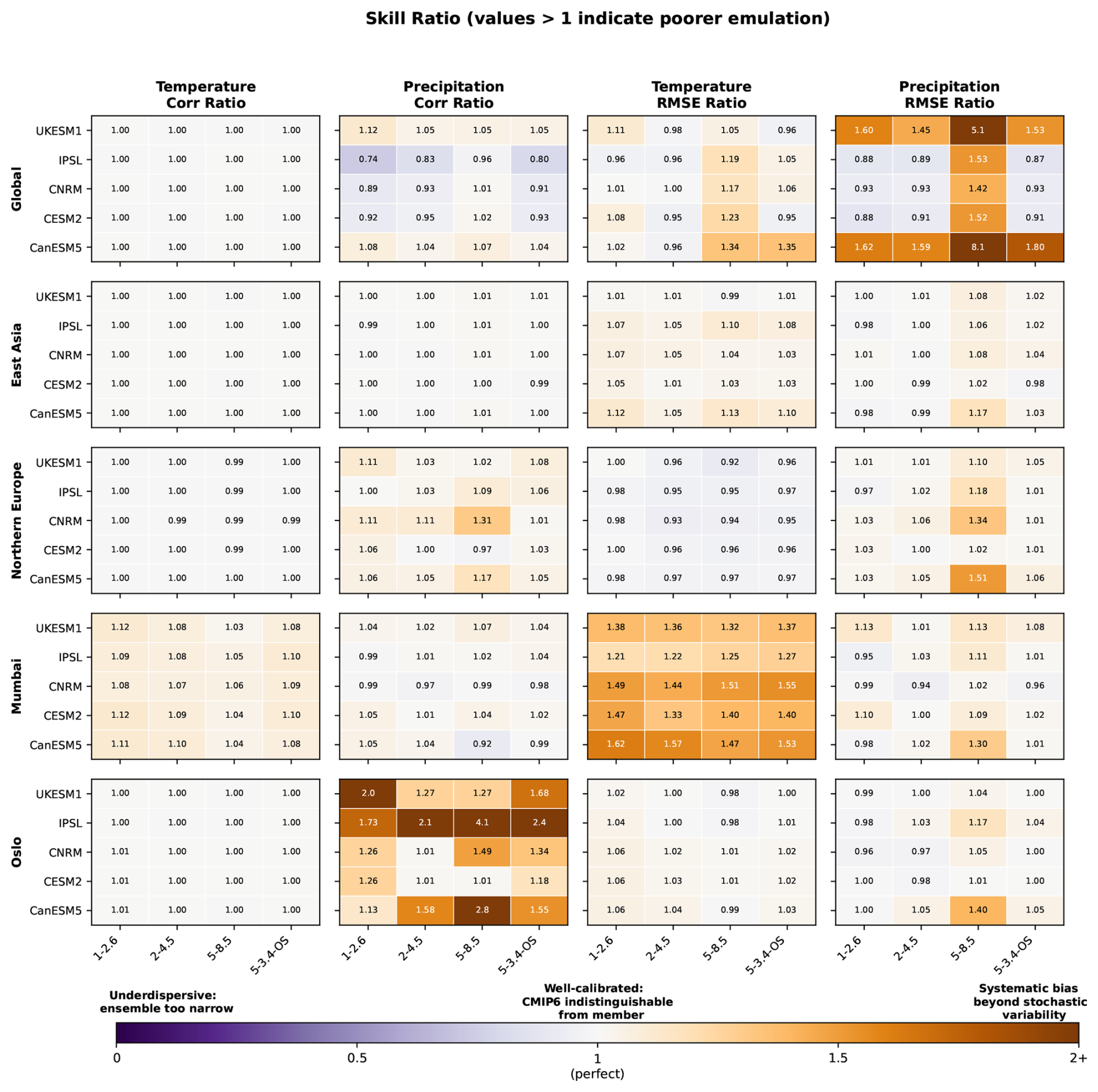
Figure 10 Skill ratio analysis for out-of-sample validation across all spatial scales (rows), models, and scenarios. Each panel shows a grid of model-scenario combinations. Skill ratios are defined such that values > 1 (orange) indicate poorer emulation for both metrics: for correlation, ratio = Member-Member $/$ Member-CMIP6; for RMSE, ratio = Member-CMIP6 $/$ Member-Member. Values near 1 (white) indicate CMIP6 is statistically indistinguishable from a METEOR ensemble member; values < 1 (purple) suggest ensemble underdispersion. Temperature ratios are consistently near unity; precipitation shows more variability, particularly at global scales where forced response bias is evident.

8 Discussion

8.1 Advantages and Integration with METEOR Core Framework

METEOR-NOISE extends the METEOR-CORE framework to monthly resolution, enabling the generation of realistic sub-annual climate variability and integrated impact metrics while preserving the multi-timescale and forcing-dependent characteristics that distinguish METEOR from conventional pattern scaling approaches.

The framework's primary strength is computational efficiency combined with interpretable statistical realism. It generates ensembles far faster than ESMs while preserving many aspects of spatial coherence, temporal persistence, and teleconnections. The decomposition into seasonal and anomaly components aids interpretability, and the PC-based approach enables calculations at multiple spatial scales without redundancy.

The temperature-modulated seasonal cycle can represent warming effects on annual cycles. This is particularly important for high-latitude regions undergoing rapid change. METEOR-NOISE is fully integrated with METEOR-CORE in a combined interface, enabling rapid generation of large climate ensembles (100+ members in under 2 min) for any scenario METEOR can emulate. Each ensemble member shares the same forced response but explores a distinct realization of internal variability, providing a direct characterization of the irreducible uncertainty in regional climate projections.

METEOR-NOISE maintains the framework's ability to represent hysteresis effects and forcing-dependent responses, which are critical for scenarios involving emission overshoots or varying forcer mixes (Good et al., 2015; Herger et al., 2015). Monthly variability generation adds very modest computational overhead while maintaining METEOR's performance advantages over ESM simulations, enabling large ensemble generation for uncertainty quantification. The temporal resolution supports sectoral applications requiring sub-annual climate information, including energy demand modeling, agricultural impact assessment, and extreme event analysis (Sillmann et al., 2013).

The framework propagates uncertainty from climate projections through to impact metrics, enabling probabilistic risk assessment that accounts for both forced climate change and natural variability. The impact assessment here is just a simple illustrative example, but the model structure provides standardized interfaces so that new sector-specific applications can be added without re-implementing the uncertainty and ensemble handling.

8.2 Limitations and Future Developments

Current limitations of METEORv1.6 include dependencies on ESM training data quality, simplified treatment of compound events, and assumptions of stationarity in some statistical relationships. These limitations are inherited from the core METEOR framework and represent areas for continued development.

The linear seasonal model works well for temperature, but application to precipitation is more challenging due to its non-Gaussian distribution and stronger seasonality – leading to the choice to represent precipitation as a static VAR model in the default configuration. Future versions should explore more robust approaches to representing seasonality across variables, including nonlinear and non-parametric methods, noting that the linear model cannot capture highly nonlinear changes in seasonality, though the temperature-interaction terms provide substantial flexibility.

The Gaussian assumption for noise is well-justified for monthly means but likely underestimates extreme event probabilities. Anderson-Darling tests and quantile–quantile (QQ) diagnostics on the fitted VARX innovations show small skew ($\left|\text{skew}\right|\le \mathrm{0.25}$ across leading modes) but systematic positive excess kurtosis of 0.5–1.4 for temperature and 0.1–0.6 for precipitation, indicating slightly heavier tails than a strict Gaussian (Fig. S18). Extensions using t-distributed innovations, GARCH-style time-varying variance, or empirical resampling of residuals could address this for applications focused on extremes. Similarly, the current impact assessment framework focuses on a limited number of validated outputs, requiring expansion to precipitation-dependent and compound event applications.

Both the PCA basis and the VARX coefficient matrices are estimated once on the full training record and applied unchanged across all scenarios. To test the stationarity assumption implicit in this choice, we refit the noise model on the early (1850–1974) and late (1976–2100) halves of the NorESM2-MM SSP2-4.5 training record, and separately on a sequence of overlapping 100-year windows spanning the full period. The leading EOFs are broadly preserved across the split-sample halves (top-10 best-match $\left|r\right|=\mathrm{0.81}$ for temperature, 0.77 for precipitation), with the first mode particularly stable ($\left|r\right|=\mathrm{0.92}$ and 0.98 respectively) but some reordering at intermediate ranks. The VARX process is stable in the aggregate. The spectral radius of the companion matrix (a single number for how quickly a perturbation to the modeled fluctuations decays; below 1 means the process is stationary, so shocks die away rather than grow) stays within 0.94–0.96 for temperature and 0.90–0.91 for precipitation across all seven rolling windows. The overall size of the two lag matrices A₁ and A₂, measured by their Frobenius norm (the square root of the summed squares of all their entries), varies by roughly 5 %–10 % for temperature and less than 5 % for precipitation.

Individual coefficients do show some drift. The self-lag of the leading temperature mode (A₁[0,0], how strongly that mode predicts its own value the following month) rises from 0.32 in the earliest window to 0.62 in the modern period. This may reflect the leading EOF progressively absorbing more of the forced warming signal in later windows, or a genuine change in the underlying persistence timescale and the present diagnostic cannot separate these interpretations. For applications with forcing beyond the training envelope, or where variability structure at specific mid-rank modes is critical, time-varying or state-dependent parameters may be required. The additive combination of forced response and variability likewise assumes independence, whereas the real climate system exhibits some nonlinearity wherein forcing can modulate variability amplitude. Full diagnostics are provided in Figs. S15 and S16.

These limitations are important to recognize but do not undermine the model's utility for most applications. Monthly mean climate on seasonal to decadal timescales, under moderate forcing scenarios, is generally well-represented. For studies requiring daily extremes or investigating potential regime shifts, more sophisticated approaches may be needed.

Future versions will explore higher temporal sampling, including daily and sub-daily climate generation, to support applications requiring extreme event statistics. Machine learning methods for temporal (Kajbaf et al., 2022; Bassetti et al., 2024) and spatial (Wang and Tian, 2022; Kheir et al., 2023; Harder et al., 2024) downscaling represent a promising avenue for enhancing resolution while preserving physical consistency with the underlying pattern scaling framework. Additionally, improvements to forcer treatment in METEOR-CORE are planned, including incorporation of the AeroGP Gaussian process regional aerosol model (Dewey et al., 2025), which provides more sophisticated representation of spatially heterogeneous aerosol forcing responses than the current linear pattern scaling approach.

8.3 Relationship to Other Climate Emulation Approaches

METEORv1.6 complements other existing climate emulation frameworks while addressing specific limitations. Compared to MESMER's monthly extensions (Nath et al., 2022; Schöngart et al., 2024), METEORv1.6 preserves forcing-dependent and time-evolving response capabilities present in METEOR v1.0.1 (Sandstad et al., 2025) while also preserving spatial covariance structures of the target model. Other recent approaches also employ impulse response formulations for spatially resolved emulation (Freese et al., 2024; Womack et al., 2025). METEOR shares the impulse response philosophy but differs in its multi-forcer decomposition and its integration of monthly variability generation with the forced response, enabling ensemble-based uncertainty quantification alongside the pattern-scaled climate signal. Relative to machine learning approaches (Watson-Parris et al., 2021; Kendon et al., 2025; Kitsios et al., 2023), METEOR-CORE provides a physically motivated impulse-response formulation with interpretable structure and significantly lower training data requirements; METEOR-NOISE extends this with a statistical variability model calibrated to reproduce the target ESM's covariance and persistence. Further, the integration of impact assessment capabilities distinguishes METEORv1.6 from purely climate-focused emulators, providing end-to-end workflows from emissions to sectoral impacts. This integration enables consistent uncertainty propagation and ensemble analysis that may be difficult to achieve with separate climate and impact modeling systems.

9 Conclusions

METEORv1.6 is lightweight enough for interactive use, with a physically motivated core (impulse-response pattern scaling) and a statistical model of sub-annual variability calibrated against ESM output. It distills ESM behavior into interpretable pattern scaling relationships while preserving the forcing-dependent and time-evolving characteristics that separate it from purely statistical approaches, which trade physical realism for speed.

The monthly extension presented here adds realistic sub-annual variability and integrated impact assessment while maintaining this balance. Validation against CMIP6 demonstrates that METEOR reproduces key statistical properties of climate variability across spatial scales, from global means to individual grid cells. The framework captures forced responses, seasonal cycles, and interannual variability with sufficient fidelity for many impact assessment applications, while generating 100-member ensembles in under two minutes on a standard laptop.

This computational efficiency supports interactive use. METEOR could act as a climate component within integrated assessment models (IAMs), supplying spatially resolved feedbacks and probabilistic impact information in real time as users vary emission pathways. Planners, policymakers, or researchers can assess climate impacts for novel scenarios without waiting for ESM simulations.

Important challenges remain beyond the current framework's scope. Nonlinear climate responses (such as potential Atlantic Meridional Overturning Circulation (AMOC) collapse or ice sheet instabilities) cannot be captured by pattern scaling approaches that assume linear superposition of forcing responses. Novel forcing scenarios, including solar radiation management interventions, require dedicated training data and potentially new model structures to represent their distinct spatial and temporal signatures (Farley et al., 2025). These current limitations represent desirable targets for future development, to increase the applicability of the framework to a wider range of questions and scenarios.

The value of emulators like METEOR lies not in reproducing the vast data volumes of initiatives like CMIP, but in rapid turnaround: they make the relationship between emission choices and impact outcomes something a user can explore directly. That is most useful where probabilistic, spatially resolved climate information is needed on demand, and where a purely statistical emulator would lose the forcing-dependent behavior that METEOR-CORE retains.