China regional 3 km downscaling based on residual Corrective Diffusion model

A fundamental challenge in numerical weather prediction is efficiently producing high-resolution forecasts. A widely adopted solution is to downscale coarser global model outputs. This study focuses on statistical downscaling, which uses historical data to learn mappings between low- and high-resolution meteorological fields. Deep learning has become a key tool for this, enabling powerful super-resolution models like diffusion models and Generative Adversarial Networks for downscaling applications. Herein, we leverage CorrDiff, a diffusion-based downscaling framework, with three key enhancements relative to its original implementation. First, the study domain is expanded to nearly 40 times the spatial extent of the original version. Second, the scope of target downscaling variables is extended beyond surface variables to incorporate upper-air variables across six pressure levels. Third, a global residual connection is integrated to further boost prediction accuracy. To produce 3 km resolution forecasts for the China region, the trained CorrDiff model is applied to 25 km global grid forecasts derived from two sources: a conventional global numerical weather prediction model and a deep learning-based weather model developed using Spherical Fourier Neural Operators. The China Meteorological Administration Mesoscale Model (CMA-MESO) is selected as the baseline for comparative evaluation. Experimental results demonstrate that the downscaled forecasts generated by our framework outperform the direct forecasts of CMA-MESO for almost all target variables, as quantified by the Mean Absolute Error metric. Specifically, forecasts of radar composite reflectivity reveal that CorrDiff, as a generative model, is capable of capturing fine-grained meteorological details, yielding more physically realistic predictions than deterministic regression-based downscaling models.

1 Introduction

Gridded meteorological forecasts are important in various fields such as transportation, energy sector, agriculture, and scientific research. In particular, high spatial resolution forecasts are crucial for local studies and risk assessment. Traditionally, global gridded forecasts are obtained from numerical weather prediction models. Generating forecasts at kilometer (km) resolution is challenging for numerical weather prediction models due to the limitation of computation time. In fact, increasing the spatial resolution leads to a quadratic or even cubic increase in the number of grid points. This results in orders-of-magnitude more floating-point operations, substantially increasing the computational cost and preventing operational forecasting systems from producing forecasts within the required time window. The most straightforward way to reduce the runtime of kilometer-scale numerical weather prediction models is to provide additional computational resources. For example, an European Centre for Medium-Range Weather Forecasts (ECMWF) team ran a 1km resolution global simulation on Summit supercomputer at the Oak Ridge National Laboratory in Tennessee. The simulations were conducted on a fraction of Summit, at a speed of about one simulated week per day, using 960 Summit nodes with 5760 MPI tasks × 28 threads, which translates into 5.4 s per model time step (Wedi et al., 2020). Currently, there are also data-driven deep learning models that generate global forecasts (Bi et al., 2022; Lam et al., 2023; Pathak et al., 2022; Chen et al., 2023). However, the resolution of current data-driven models generally ranges from 10 to 25 kilometers. To generate high-resolution forecasts, a practical approach is to derive regional high-resolution predictions by applying a downscaling technique to the low-resolution outputs of global models.

Downscaling methods can be categorized into three types: dynamical downscaling, statistical downscaling, and combined methods. Dynamical downscaling, similar to numerical weather prediction models, is based on a set of atmospheric dynamical equations. It derives high-resolution forecasts by solving these equations using initial and lateral boundary conditions provided by global models. Statistical downscaling establishes statistical relationships between low-resolution variables of global models and high-resolution variables using historical data. These relationships are then applied for future forecasting. Compared to dynamical downscaling, statistical downscaling offers advantages, including simpler implementation, lower computational cost, and potentially higher accuracy (Legasa Rios et al., 2026; Diez et al., 2005).

Many machine learning models have been applied for statistical downscaling, such as multiple linear regression (Schoof and Pryor, 2001), support vector machine (Chen et al., 2010), random forest (Davy et al., 2010), and artificial neural networks (Laddimath and Patil, 2019). Among these models, artificial neural networks, which have evolved into deep learning (Sun et al., 2024), are likely the most promising approach.

The fast development in deep learning over the past decade has led to numerous active research areas, including super-resolution in computer vision. Various high-performance super-resolution models have been proposed, such as Generative Adversarial Networks (GANs) and diffusion models. Super-resolution is similar to downscaling: the input for both is a low-resolution grid, and the output is a high-resolution grid. However, there is also a difference between super-resolution and downscaling: the goal of super-resolution is to generate visually realistic images, while meteorological downscaling must ensure accuracy and physical consistency. Given the similarity between super-resolution and downscaling, many researchers have investigated the application of such super-resolution models to downscaling (Watt and Mansfield, 2024; Addison et al., 2022). Beyond generative super-resolution models, convolutional neural networks (CNNs) have also been widely adapted for downscaling workflows (Vandal et al., 2017, 2019). A core limitation of vanilla CNNs lies in their constrained receptive fields, which hinders the modeling of long-range spatial dependencies indispensable for weather forecasting. To mitigate this issue, SwinIR, a transformer-based architecture built upon the Swin transformer backbone (Liu et al., 2021), has been introduced for downscaling. It unites two complementary strengths: the hierarchical shifted-window design of transformers for capturing long-distance spatial correlations, and the local feature extraction capability intrinsic to CNNs (Liang et al., 2021; Zhong et al., 2024; Li et al., 2025). Apart from repurposed computer vision models, numerous studies have also designed bespoke neural networks specialized for meteorological downscaling (Wu et al., 2024).

This work investigates a diffusion-based downscaling model named Corrective Diffusion (CorrDiff) (Mardani et al., 2025). CorrDiff is a two-step approach that includes the training of a regression model and the training of a diffusion model to improve the predictions of the regression model. In Mardani et al. (2025), CorrDiff is applied to the Taiwan region, the resolution of the inputs is 25 km and the resolution of the outputs is 2 km. The size of the 2 km high-resolution grid is 448 × 448. In this study, we apply CorrDiff on the China region, the resolutions of the inputs and the outputs are 25 and 3 km respectively. The size of our 3 km high-resolution grid is 1600 × 2400, which is nearly 20 times the size in Mardani et al. (2025). Our models are trained on reanalysis data, including 25 km ECMWF Reanalysis v5 (ERA5) (Hersbach et al., 2020) (as low-resolution inputs of the downscaling models) and 3 km reanalysis data (as high-resolution labels) that are produced by China Meteorological Administration Regional Reanalysis Atmospheric System (CMA-RRA) (Xu et al., 2026). In contrast to Mardani et al. (2025), which focuses mainly on surface variables, in this work multiple variables are considered for downscaling, including surface variables and variables at six pressure levels. The prediction of radar composite reflectivity is also investigated. Different combinations of input and output variables are examined in order to understand the intervariable dependencies in the downscaling task. By connecting our downscaling models to global forecasts, 3 km regional forecasts for the China region are obtained, which are evaluated through comparison with the China Meteorological Administration Mesoscale Model (CMA-MESO). CMA-MESO is a high-resolution regional numerical weather prediction model that generates 3 km and 1km resolution forecasts of the China region. Two global forecasts are considered: the China Meteorological Administration-Global Forecast System (CMA-GFS) and Sphere Fusion Forecast (SFF), which is a deep learning-based weather model. The experimental results demonstrate that, for the Mean Absolute Error (MAE), our forecasts generally outperform those of CMA-MESO for the target variables. Our assessment of the uncertainty estimated by CorrDiff shows that, for any downscaled variable, the uncertainty is correlated with the accuracy. For the prediction of radar reflectivity, our results show that deterministic models usually have a severe over-smoothing problem, while CorrDiff can generate realistic small-scale features that are similar to reanalysis data.

This paper is organized as follows. Section 2 introduces the high-resolution reanalysis data used for training and the CorrDiff framework. Section 3 presents the training setup, the evaluation on the validation data, covering prediction errors and the properties of the uncertainty estimated by our models, and assesses the 3 km forecasts generated by applying our models to the forecasts of global models (CMA-GFS and SFF). Section 4 draws conclusions and discusses future directions.

2 Data and Method

2.1 3 km Resolution Reanalysis Data

The 3 km resolution reanalysis data used in this study are produced by CMA-RRA. CMA-RRA was developed by the CEMC and is based on the 3 km rapid refresh cycling assimilation and forecast system of CMA-MESO. It has a spatial resolution of 3 km and a temporal resolution of 1 h, and covers the same region as CMA-MESO: 10–60.1° N, 70–145° E.

CMA-RRA comprises multiple modules, including observational data preprocessing and quality control, three-dimensional variational data assimilation, cloud analysis, incremental analysis update (IAU), large-scale background field initialization, multi-scale hybrid assimilation, digital filtering, and mesoscale model forecasting. CMA-RRA operates through an inner analysis cycle and an outer cycle. The inner analysis cycle uses an hourly assimilation-forecast cycle and the hydrometeor variables are not updated during the analysis process. Using the results from the inner cycle analysis, the outer cycle conducts cloud analysis using networked Doppler weather radar 3D reflectivity products and Fengyun geostationary meteorological satellite cloud products. This process generates cloud analysis and hourly precipitation products.

2.2 Problem Formulation

$\mathit{\{}{x}_i\in {\mathbb{R}}^{c_{\mathrm{in}}\times p\times q}\mid i\in \mathit{\{}\mathrm{1},\mathrm{\dots },N\mathit{\left\}}\mathit{\right\}}$ and $\mathit{\{}{y}_i\in {\mathbb{R}}^{c_{\mathrm{out}}\times m\times n}\mid i\in \mathit{\{}\mathrm{1},\mathrm{\dots },N\mathit{\left\}}\mathit{\right\}}$ represent 25 and 3 km resolution meteorological data over the China region, respectively. c_in (c_out) is the number of variables of the 25 km (3 km) data. p and q (m and n) represent the number of grid points in the meridional and zonal directions respectively of 25 km (3 km) data. N is the number of training samples. In this work, p=192, q=288, m=1600, and n=2400. The 25 km data correspond to the region 12.25–60° N, 70–141.75° E and the 3 km data correspond to the region 12.13–60.1° N, 70–141.97° E. Different combinations of c_in and c_out are investigated, which will be discussed in Sect. 3.1. The objective is to train a deep learning model to predict y_i from x_i.

In the case of using a regression model (in this paper, regression models refer to deterministic deep learning models, such as UNet), first, the input x_i is interpolated onto the 3 km resolution grid by bilinear interpolation, which is denoted as bilinear(x_i), then bilinear(x_i) is fed into a deep learning model that can be represented by a function $f:{\mathbb{R}}^{c_{\mathrm{in}}\times p\times q}\mapsto {\mathbb{R}}^{c_{\mathrm{out}}\times m\times n}$. f(bilinear(x_i)) is the prediction of the 3 km grid that corresponds to x_i. The training of this deep learning model is to find parameters of f that minimize a loss function quantifying the distance between f(bilinear(x_i)) and y_i for $i\in \mathit{\{}\mathrm{1},\mathrm{\dots },N\mathit{\}}$.

In this work, we also use diffusion models. Generally, a diffusion model involves two processes: noising and denoising. Noising is the process that progressively adds noise to a clean image until the image becomes random noise. Denoising is the process that transforms random noise into a structured image. Basically, the training of a diffusion model can be considered as the training of a denoising model. In the case of using diffusion models for downscaling, the low-resolution data are also fed into the diffusion models. Such models are also known as conditional diffusion models. The overall inference process of a conditional diffusion model for downscaling can be represented by a function $f:{\mathbb{R}}^{c_{\mathrm{in}}\times p\times q},E\mapsto {\mathbb{R}}^{c_{\mathrm{out}}\times m\times n}$, which is a conditional sampling function of the probability of the 3 km resolution data given a 25 km resolution input. E represents the set of random noise that follows a certain distribution (which normally follows the normal distribution). Note that this function f is highly complex because the denoising process contains multiple steps that progressively decrease the noise level. For more details on diffusion models, see Ho et al. (2020).

2.3 Corrective Diffusion Model

This section briefly introduces the Corrective Diffusion (CorrDiff) model, for more details see Mardani et al. (2025). The code implementation is based on PhysicsNeMo (https://github.com/NVIDIA/physicsnemo, last access: 9 February 2026). The training of CorrDiff has two steps. In the first step, we train a regression model (UNet), denoted as f, to minimize a loss function between its predictions f(bilinear(x_i)) and the targets y_i for all $i\in \mathit{\{}\mathrm{1},\mathrm{\dots },N\mathit{\}}$. In the second step, we train an Elucidated Diffusion Model (EDM) (Karras et al., 2022) to correct the predictions made by f. We denote the overall inference process of EDM by a function g. After training, the CorrDiff prediction ${\widehat{y}}_i$ for the target y_i is given by ${\widehat{y}}_i=g\left(\mathrm{bilinear}\right(x_i),f(\mathrm{bilinear}\left(x_i\right)),\mathit{ϵ})+f\left(\mathrm{bilinear}\right(x_i\left)\right)$, where ϵ is a random noise sampled from a standard normal distribution. By sampling multiple random noises, a CorrDiff model generates an ensemble of predictions, thereby producing a probabilistic prediction of y_i.

Following Mardani et al. (2025), we use a specific architecture of UNet (Karras et al., 2022) for both the regression (first step) and diffusion (second step) networks. This architecture has 6 encoder and decoder layers, and it incorporates attention mechanisms and residual connections within its structure.

Figure 1 Illustration of the overall architecture of one of our trained CorrDiff models.

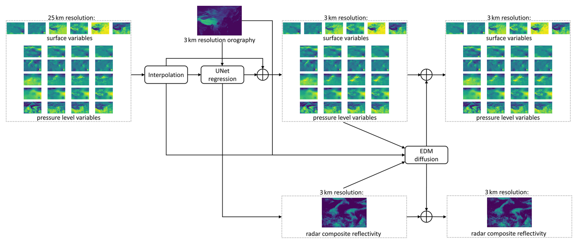
Figure 1 shows the overall architecture of one of our trained CorrDiff models. Our regression networks differ slightly from the models in Mardani et al. (2025): for the downscaling of a variable, assuming that $x_i^u$ and $y_i^v$ correspond to this variable (where $x_i^u\in {\mathbb{R}}^{p\times q}$ is a channel of x_i, and $y_i^v\in {\mathbb{R}}^{m\times n}$ is a channel of y_i), instead of directly predicting $y_i^v$, we predict the residual $y_i^v-\mathrm{bilinear}\left(x_i^u\right)$, because our experimental results show that this residual learning strategy could accelerate convergence speed and improve accuracy for the downscaling task. In contrast to Mardani et al. (2025) which only considers the downscaling of surface variables, this work also investigates the downscaling of pressure level variables. An additional input (3 km resolution orography) is included in our models as well. The implementation of our models is based on the code provided in Mardani et al. (2025).

As stated in Mardani et al. (2025), the development of CorrDiff was motivated by the limitations of using conditional diffusion models for downscaling. It is assumed that there is a significant distribution shift between low-resolution and high-resolution data that hinders the learning process. To avoid this problem, the generation is decomposed into two steps. The first step aims to predict the conditional mean using regression (UNet), and the second step learns a correction using a diffusion model.

3 Experiments and Results

3.1 Training Setup

For the training of CorrDiff, we use 25 km ERA5 as input data and 3 km reanalysis data as target data. The size of the 25 km input data is 192 × 288 covering the region 12.25–60° N, 70–141.75° E, and the size of the 3 km target data is 1600 × 2400 covering the region 12.13–60.1° N, 70–141.97° E. The mismatch in spatial resolution (25 km vs. 3 km) (non-divisibility of 25 by 3) results in minor misalignment between input and target region, which could potentially reduce the accuracy on the boundary. We use the data from 2019 to 2022 as the training set, choosing eight time points each day: 00:00, 03:00, 06:00, 09:00, 12:00, 15:00, 18:00, and 21:00 UTC. In total, the training set contains 11 688 samples.

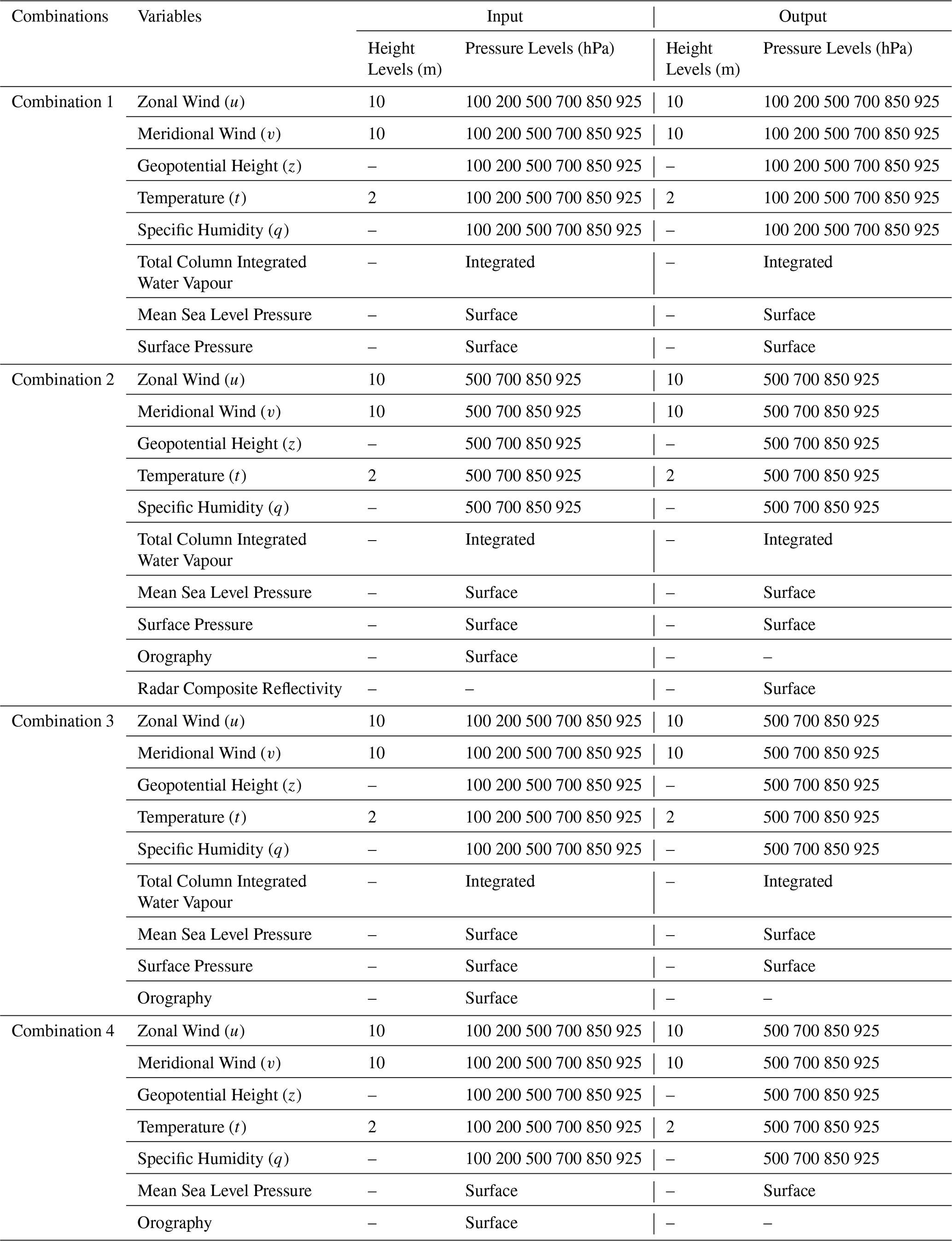
For deep learning models, we have the flexibility to select various combinations of variables as inputs and outputs. In this work, we investigate four distinct input/output configurations, detailed in Table 1. For example, for a model that corresponds to Combination 4, the input has 35 variables (c_in=35) and the output has 24 variables (c_out=24).

Table 1 Different input/output variable combinations.

3.2 Training Results on the Validation Set

The data from January, April, July, and October 2023 are used as the validation set. We select eight time points each day as in the training set: 00:00, 03:00, 06:00, 09:00, 12:00, 15:00, 18:00, and 21:00 UTC. In total, there are 984 samples in the validation set.

3.2.1 Regression Models

Five regression models have been trained, denoted as Regression 1, Regression 2, Regression 3-1, Regression 3-2, and Regression 4. Regression 1, 2, and 4 correspond to Combination 1, 2, and 4 in Table 1, respectively. Regression 3-1 and 3-2 correspond to Combination 3.

• Regression 1 is the first trained model. It incorporates the most variables to test the feasibility of downscaling multiple variables with a single model. In order to ensure sufficient model complexity, we increase the size of Regression 1 such that only one sample can be computed at one time on a single NVIDIA H20 GPU with the use of checkpointing. The UNet embedding size of Regression 1 is [128, 256, 512, 512, 1024].

• Regression 2 builds upon Regression 1 by adding orography as an additional input variable in order to increase accuracy. Furthermore, radar composite reflectivity is added as an output for Regression 2, while high-altitude variables (100 and 200 hPa) are removed for both input and output, since high-altitude forecasting is not our main focus.

• Regression 3-1 modifies Regression 2 by excluding radar reflectivity as an output but reintroducing the 100 and 200 hPa variables as inputs, under the assumption that additional inputs would not harm performance. Regression 3-2 is a smaller version of Regression 3-1 with reduced model complexity, designed to test if a reduced-size network could maintain comparable accuracy. The UNet embedding size of Regression 3-2 is [32, 64, 128, 256, 256].

• Regression 4 is implemented based on Regression 3-1 but excludes total column integrated water vapour and surface pressure to ensure compatibility with SFF (see Sect. 3.3.1), which does not produce these two variables. For Regression 1, 2, 3-1 and 3-2, a batch size of 64 is used to ensure stable gradient estimations, while for Regression 4, we experimented with a smaller batch size (a batch size of 8) to explore its effects on training dynamics, acknowledging that this modification would decrease the time per step due to our use of gradient accumulation.

The validation curves for the five regression models are shown in Fig. 2. Since only Regression 2 predicts radar reflectivity, the validation curve of radar reflectivity is excluded due to the absence of comparative benchmarks.

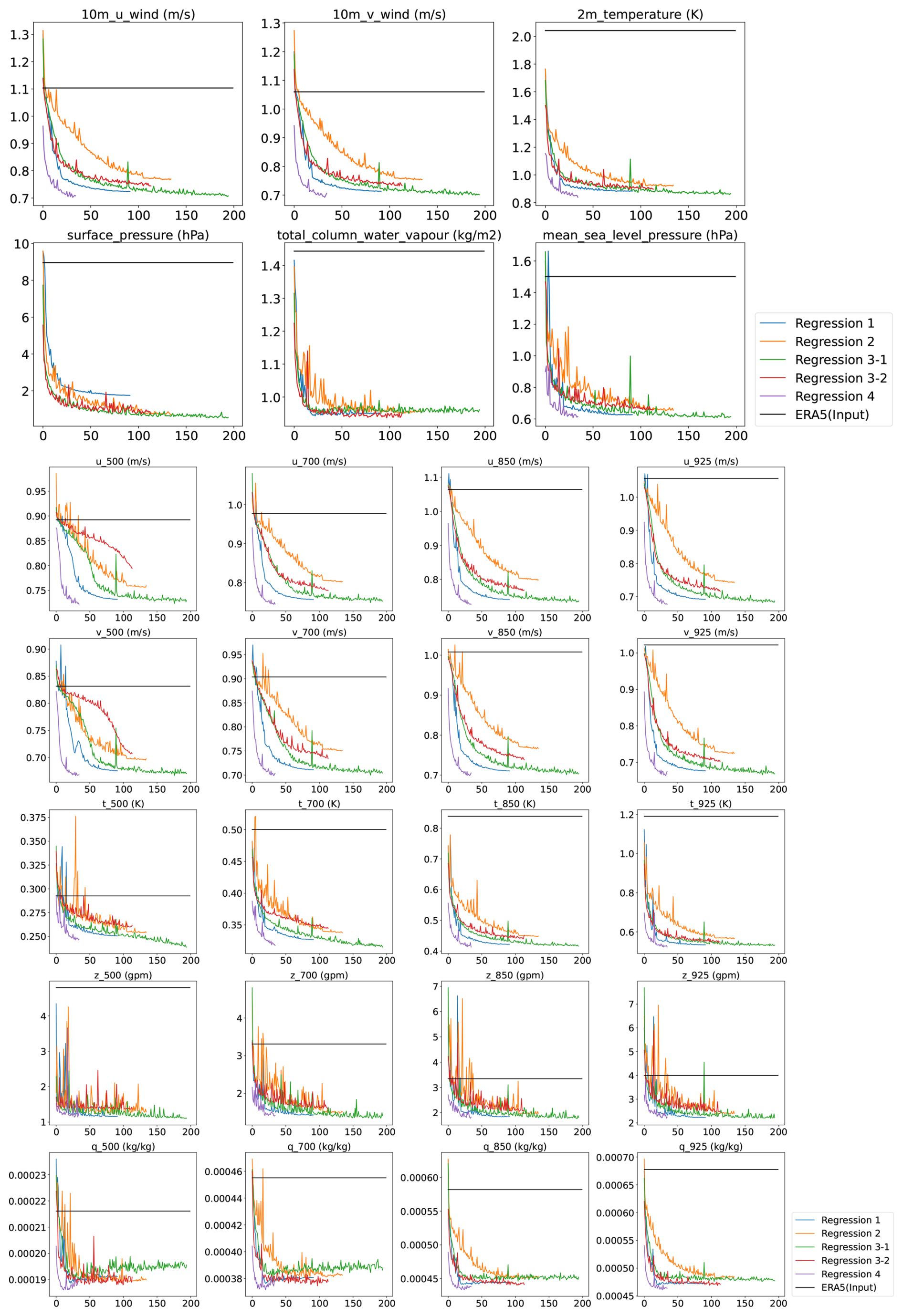
Figure 2 Validation curves of regression models for surface variables (top) and pressure level variables (bottom). Each subplot corresponds to a target variable. The curves plot the Mean Absolute Error (y-axis) against the number of training epochs (x-axis). ERA5 is used as the ground truth.

In each subplot, the black horizontal line denotes the MAE of the ERA5 input for a variable (MAE between $\mathrm{bilinear}\left(x_i^u\right)$ and $y_i^v$ for all (x_i, y_i) in the validation set, where $x_i^u$ and $y_i^v$ correspond to this variable). After the first few epochs, all validation curves remain below the black line, indicating that all regression models consistently outperform simple interpolation. The validation curves exhibit distinctive patterns between variables. For example, the validation curves of the 10 m wind decrease with a progressively decreasing rate of decline, while, for the 500 hPa wind, the rate of decline decreases at first and increases after several epochs. In addition, all validation curves display a globally decreasing trend, except for specific humidity (q), suggesting the existence of overfitting for this variable. These inter-variable differences imply that employing variable-specific embedding methods could potentially enhance both the convergence speed and model accuracy.

The comparative analysis between the validation curves of Regression 1 and Regression 2 shows that Regression 1 significantly outperforms Regression 2 on all variables except surface pressure. It is important to note that we did not exhaustively explore all combinations, for example, between Combination 1 and Combination 2, we can also examine another combination that does not include radar composite reflectivity as well as the 100 and 200 hPa variables. We assume that the impact of the 100 and 200 hPa variables on the downscaling of other variables exists but is minor and that including orography as an input should not harm the performance. Therefore, the results suggest that integrating radar reflectivity inference with downscaling in a single model might compromise downscaling accuracy, and adding orography to the inputs increases the accuracy of surface pressure.

As expected, Regression 3-1, which excludes radar composite reflectivity but includes orography as an additional input, outperforms both Regression 1 and 2. The reduction of model complexity in Regression 3-2 causes a performance degradation for most variables, indicating that this reduced version does not have sufficient model complexity.

The curves of Regression 4 are significantly lower than those of the previous models. This improvement can be attributed to two potential reasons: first, the smaller batch size may provide better gradient estimations for this downscaling task; second, excluding surface pressure and total column integrated water vapour likely reduces task complexity, freeing up model capacity for the remaining variables. Consequently, further adjustment to the batch size and a more sophisticated selection of input/output variables could lead to additional performance gains.

In the rest of this paper, we mainly focus on analyzing Regression 2 and Regression 4, as only Regression 2 can output radar composite reflectivity, and Regression 4 is compatible with SFF and has the highest accuracy on the validation set.

Table 2 MAE on the validation set. Bold formatted values denote the lowest MAE (i.e., best performing result) among all compared models (Regression and CorrDiff) for each respective variable.

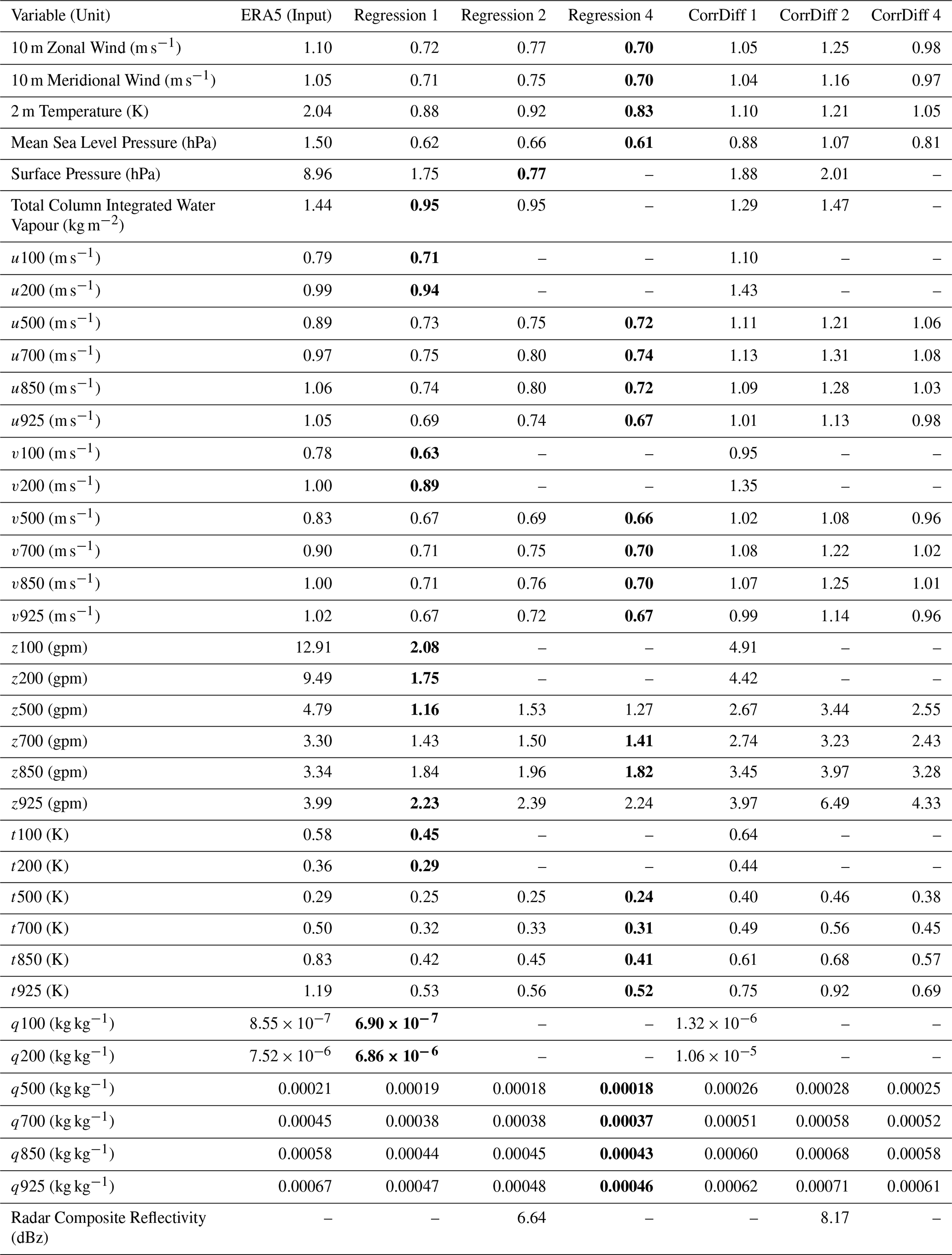
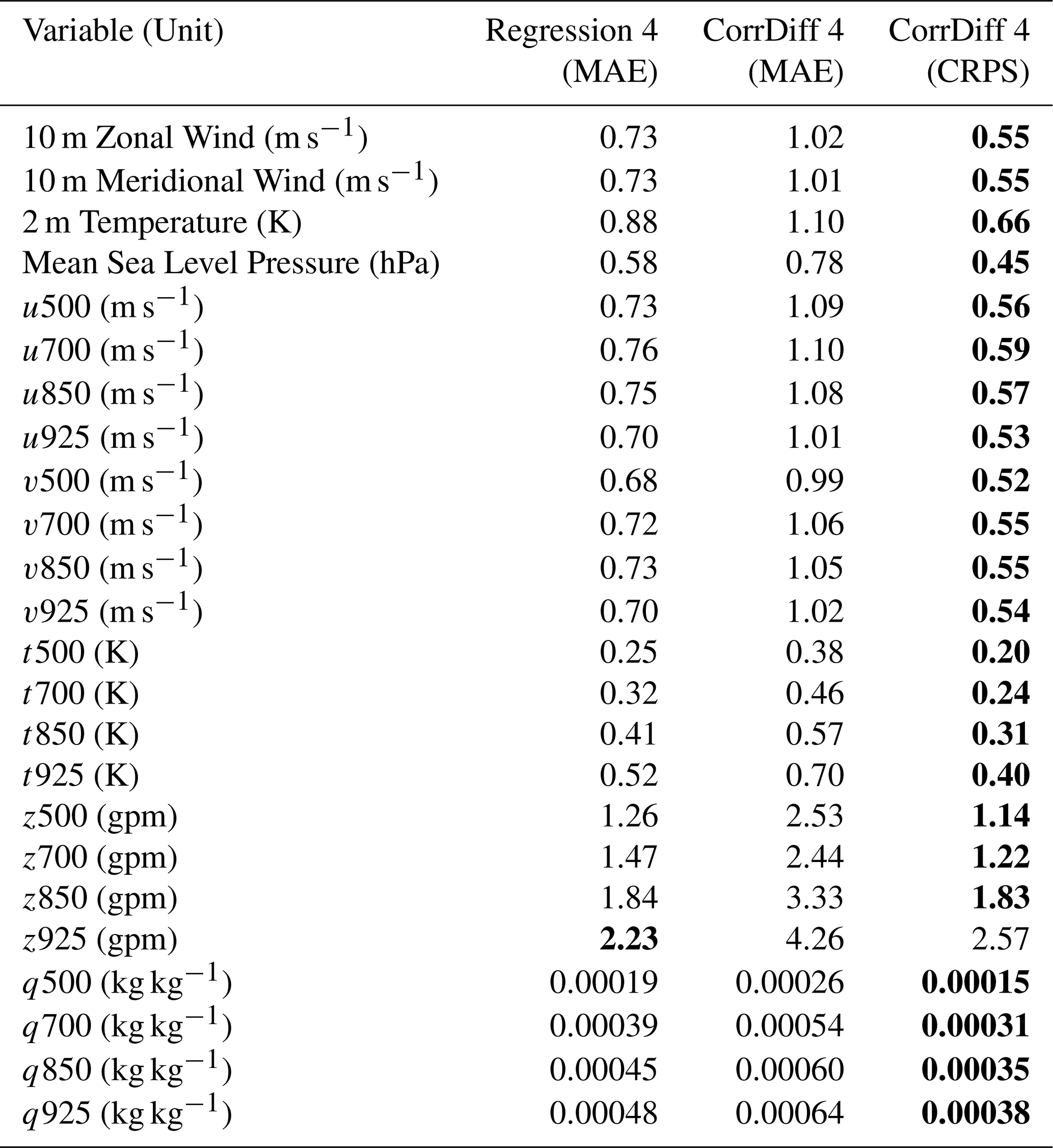
Table 3 MAE and CRPS for the data at 00:00 and 12:00 UTC on the first day of each month in 2023 of Regression 4 and CorrDiff 4.

3.2.2 CorrDiff Models

The CorrDiff models that correspond to Regression 1, 2, and 4 are denoted as CorrDiff 1, 2, and 4, respectively. Their MAE scores on the validation set are presented in Table 2. All reported MAE scores for the CorrDiff models are computed using a single sample. Our results indicate that the MAE scores of the regression models are consistently lower than those of the CorrDiff models. In fact, the degradation in MAE of the CorrDiff models compared to that of the regression models is also reported in Mardani et al. (2025). As stated in Mardani et al. (2025), the degradation is expected as the diffusion models optimize the Kullback-Leibler divergence as opposed to the regression models that minimize the MSE loss. Following Mardani et al. (2025), we also compute the Continuous Ranked Probability Score (CRPS) (Hersbach, 2000), see Table 3. CRPS can be considered as a generalization of MAE for probability prediction. Since the computation of CRPS is slow with our current implementation (primarily due to the large grid size), we select a more restricted set of time points for its calculation: 00:00 and 12:00 UTC on the first day of each month in 2023 and we only focus on CorrDiff 4. As expected, the CRPS values are generally the lowest.

Some examples of the predictions of Regression 4 and CorrDiff 4 are given in Fig. 3. The local patterns that do not occur in the low-resolution data (top-right) are captured by both the regression and CorrDiff models. An example of typhoon downscaling is given in Fig. 4. The typhoon structures generated by both Regression 4 and CorrDiff 4 are more similar to the 3 km reanalysis data compared to ERA5. The comparison between the outputs of Regression 4 and CorrDiff 4 reveals that the CorrDiff models generate more high-frequency details.

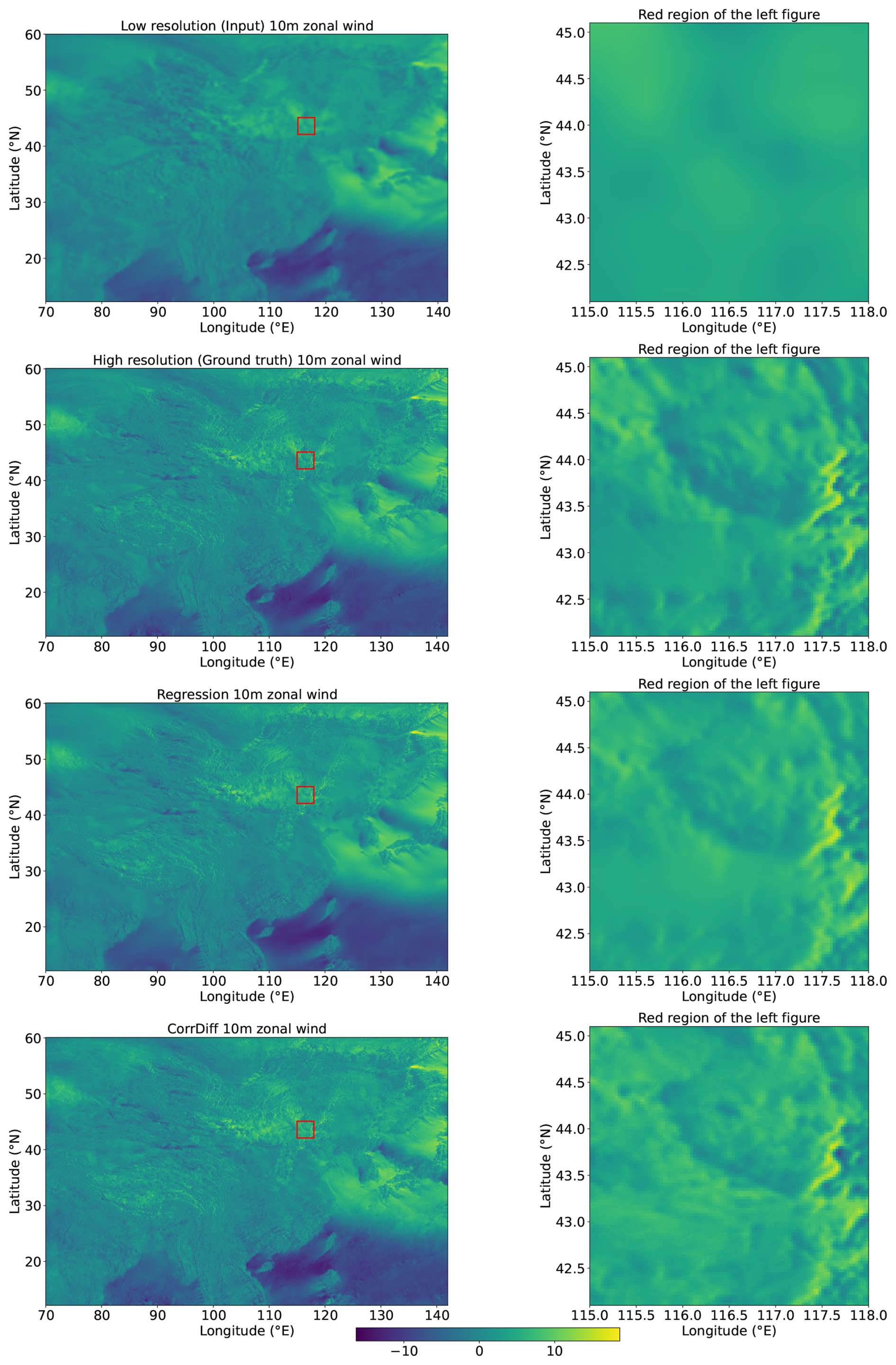
Figure 3 Illustration of the 10 m zonal wind inference of Regression 4 and CorrDiff 4 for data from 1 December 2023 00:00 UTC. Each figure on the right is a zoomed view of the red box area in the left figure.

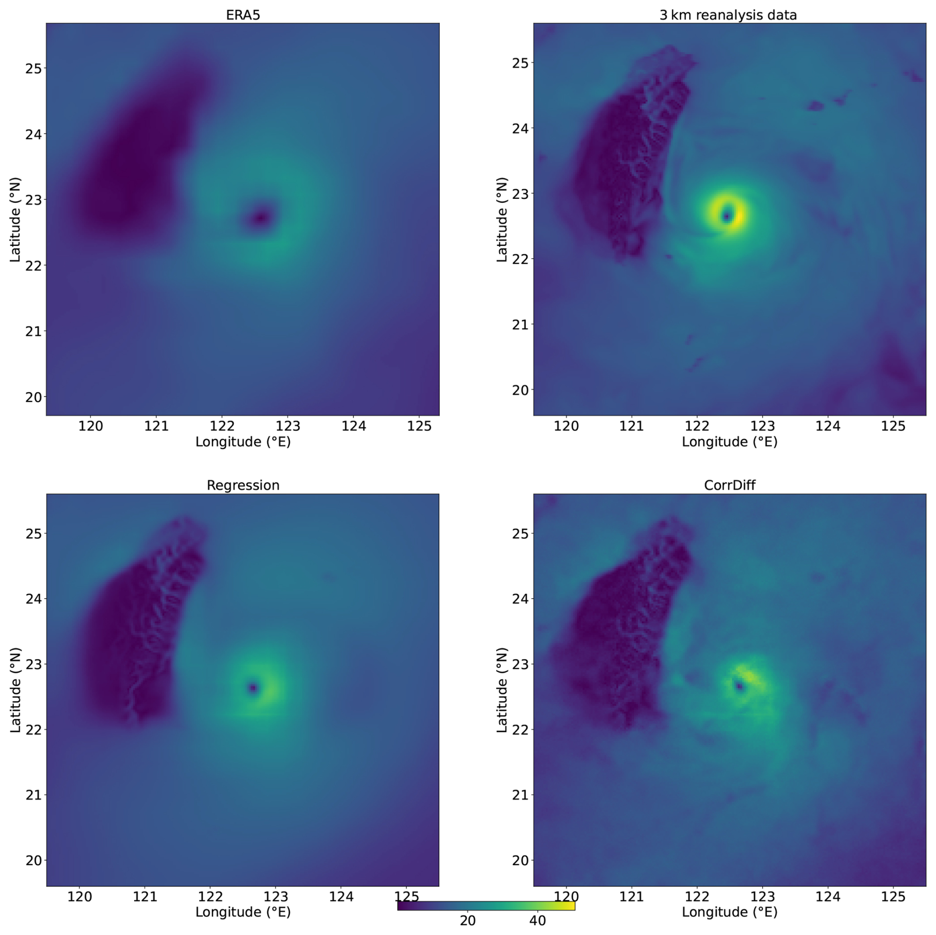
Figure 4 Illustration of the downscaling of Typhoon Haikui on 3 September 2023 00:00 UTC by Regression 4 and CorrDiff 4. Figures show the 10 m wind speed.

To further investigate whether CorrDiff learns physically meaningful corrections or merely injects stochastic noise, we analyzed the correction fields generated by the diffusion model. Figures 5 and 6 illustrate the difference between CorrDiff and regression predictions (CorrDiff minus regression), where red and blue regions represent positive and negative corrections, respectively. We observe that the corrections are predominantly positive or negative for some variables, such as 2 m temperature, while positive and negative corrections are nearly balanced for other variables such as 10 m wind. The magnitudes of the corrections also exhibit clear spatial dependence. For 10 m wind, corrections are notably stronger over the Qinghai–Tibet Plateau and oceanic regions than over other areas. For radar composite reflectivity, the corrections are concentrated in limited regions and remain close to zero elsewhere. These characteristics indicate that the diffusion model does not simply add random perturbations uniformly across the domain. Instead, it learns spatially organized corrections that are associated with meteorologically active regions and variables with strong small-scale variability. At the same time, we also observe that, for some relatively smooth variables and in certain regions, part of the correction field resembles stochastic noise. This suggests that the current CorrDiff framework may over-correct weak residual signals, which could partially explain the degradation in deterministic MAE. We therefore believe that diffusion-based corrections should be applied selectively rather than uniformly across all variables and regions. Developing region-aware or variable-dependent correction strategies is an important direction for future work and may further improve deterministic prediction accuracy while preserving the ability of CorrDiff to generate realistic fine-scale structures and probabilistic forecasts.

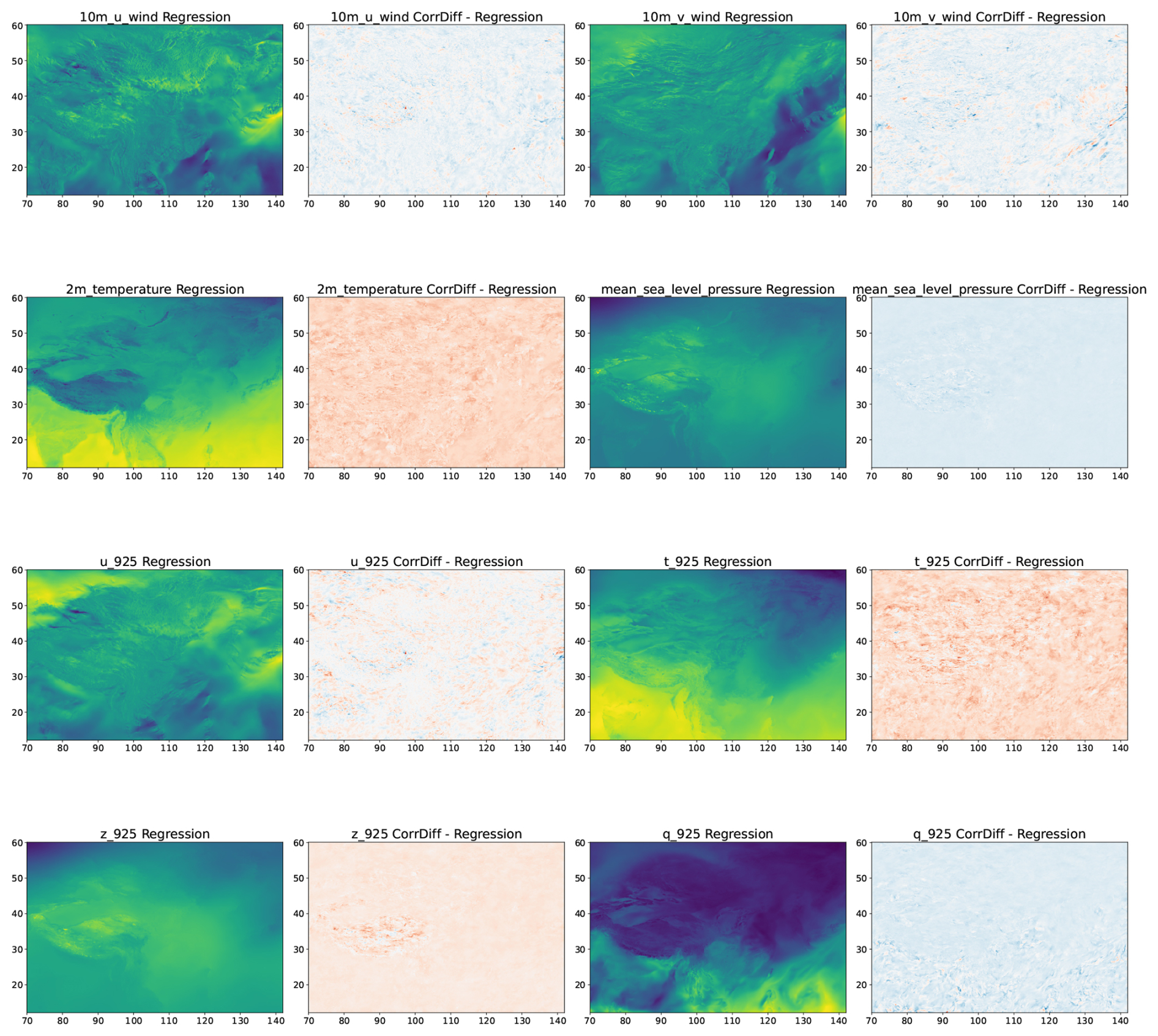
Figure 5 Outputs of Regression 4 and the difference between CorrDiff 4 and Regression 4 (CorrDiff 4 minus Regression 4) for some downscaling variables. In the figures that display the difference, red corresponds to positive values and blue corresponds to negative values. The darker the color, the larger the absolute value. The input data are ERA5 from 2 March 2023 00:00 UTC.

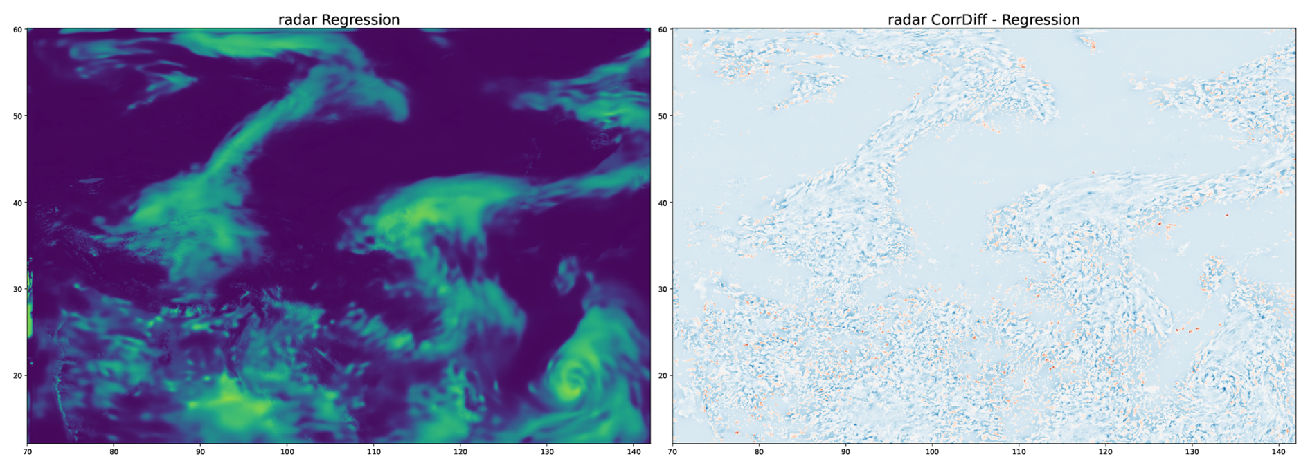
Figure 6 Outputs of Regression 2 and the difference between CorrDiff 2 and Regression 2 (CorrDiff 2 minus Regression 2) for radar composite reflectivity. In the figure that displays the difference, red corresponds to positive values and blue corresponds to negative values. The darker the color, the larger the absolute value. The input data are ERA5 from 30 July 2023 00:00 UTC.

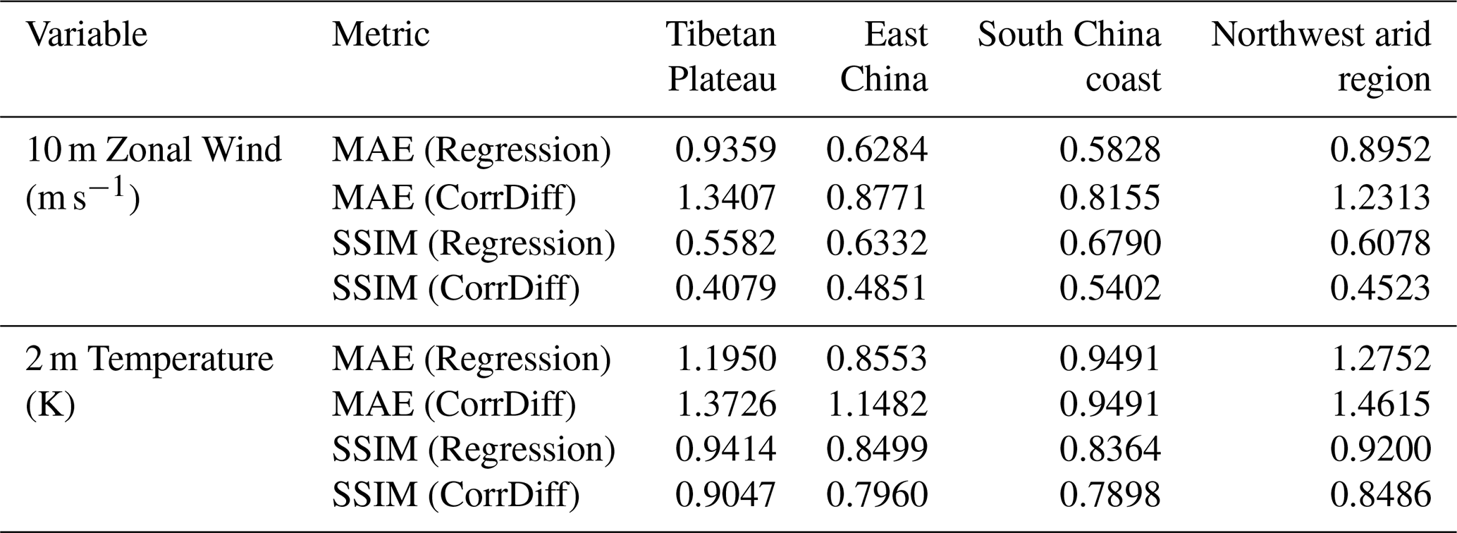
The CorrDiff framework assumes a globally shared residual correction model, which may appear to implicitly rely on a spatially stationary residual distribution. However, in the context of large-scale regional downscaling over China, this assumption is only an approximation. The underlying meteorological fields exhibit strong spatial heterogeneity due to complex topography, including the Tibetan Plateau, coastal regions, deserts, and inland basins. As a result, the residual between low-resolution inputs and high-resolution targets is not strictly stationary across the domain. To investigate this issue, we perform a spatially stratified error analysis over different geographical and vertical regions. As shown in Fig. 7 and Table 4, the distribution of prediction errors exhibits clear regional dependence. In particular, higher errors are observed over complex terrain such as the Tibetan Plateau, while relatively lower errors are found in flat inland regions. Similar spatial variability is also observed across different pressure levels. Although a single neural network is used across the entire domain, the CorrDiff model is conditioned on spatially varying inputs, including interpolated low-resolution atmospheric fields and high-resolution orography. This conditioning mechanism induces an implicit partitioning of the residual space, allowing the model to learn location-dependent correction patterns without explicitly defining regional experts. Therefore, while strict spatial stationarity does not hold, the learned residual distribution can be interpreted as a conditional, state-dependent stochastic process. These results suggest that the CorrDiff framework does not enforce spatial homogeneity in practice, but instead learns a data-driven approximation of spatially varying residual statistics through conditional generation.

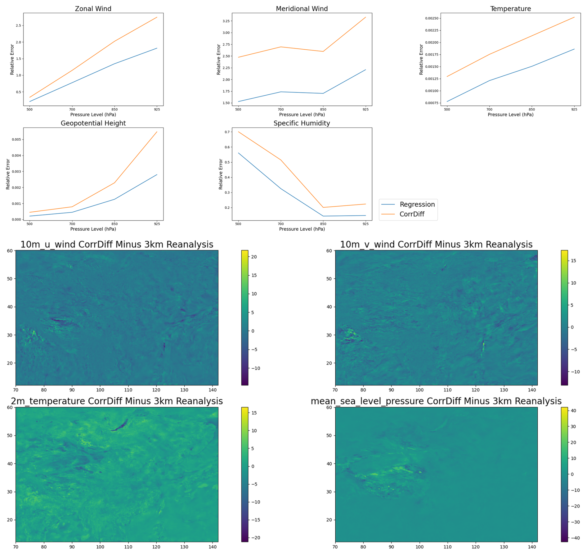
Figure 7 Top: relative error at different pressure levels, based on data from 00:00, 06:00, 12:00, and 18:00 UTC on 1, 2, and 3 March 2023. Bottom: spatial distribution of error, based on data from 00:00 UTC on 1 March 2023. Downscaling models are Regression 4 and CorrDiff 4.

Table 4 MAE and the structural similarity index measure (SSIM) of 10 m zonal wind and 2 m temperature downscaled by Regression 4 and CorrDiff 4, evaluated over four regions: Tibetan Plateau (25.99–40° N, 70–104.68° E), East China (21.01–38.23° N, 112.99–122.98° E), South China coast (18.01–25.51° N, 95.98–118° E) and Northwest arid region (34.99–49.99° N, 73–106° E), using data from 00:00, 06:00, 12:00, and 18:00 UTC on 1, 2, and 3 March 2023.

All models in this study are trained on eight NVIDIA H20 GPUs. The wall-clock training time per epoch differs substantially across model configurations: Regression 1 and Regression 3-1 take around 4 h each; Regression 2 requires roughly 3.6 h; Regression 3-2 takes approximately 1.3 h; Regression 4 needs about 3.3 h; and every CorrDiff variant (1, 2, 4) consumes nearly 2 h per training epoch. The storage size of exported PyTorch checkpoint files also varies noticeably. Regression 1, Regression 2 and Regression 3-1 produce 3.35 GB model files; Regression 3-2 yields a much smaller checkpoint of 312 MB; Regression 4 results in a 2.74 GB file; while all CorrDiff models (1, 2, 4) generate 6.21 GB checkpoints. The number of model parameters is: Regression 1, 2, and 3-1 have 8.99×10⁸; Regression 3-2 has 8.18×10⁷; Regression 4 has 7.35×10⁸; and CorrDiff 1, 2, and 4 have 1.67×10⁹. We further report the peak reserved GPU memory measured under a single batch size per GPU: Regression 1, 2 and 3-1 peak at ∼ 85 GB; Regression 3-2 occupies only 20 GB at maximum; Regression 4 reaches a peak memory footprint of 65 GB; and CorrDiff 1, 2 and 4 record peak memory usages of 77, 70 and 60 GB, respectively. The UNet embedding channel dimensions are configured as follows. Regression 1, 2, 3-1, alongside all CorrDiff models (1, 2, 4), adopt the embedding size sequence [128, 256, 512, 512, 1024]. Regression 3-2 uses a smaller sequence [32, 64, 128, 256, 256], whereas Regression 4 is built with [96, 192, 384, 768, 768].

3.2.3 Uncertainty Estimation based on CorrDiff

A key advantage of diffusion models is that they can provide probabilistic predictions. The variance of the N-member ensemble predictions from CorrDiff can be used to quantify the predictive uncertainty. Fig. 8 illustrates the correlation between the absolute errors of Regression 4 and the variance of the 20-member CorrDiff 4 predictions for the data from 1 October 2023 00:00 UTC. The shape of the point sets reveals that grid points that exhibit both high absolute error and very low variance are rare, suggesting that low variance is a potential indicator of high accuracy. Due to the high density of points, it is difficult to clearly see the distribution of the points. So we plot three horizontal black lines that mark the 75th, 50th, and 25th percentile of the variance. These percentiles partition the data into four groups, each representing a different level of uncertainty (for example, points above the 75th percentile have the highest uncertainty). The MAE for each group is computed and annotated within the subplots. For all variables, the MAE decreases markedly as the variance decreases across these four groups. The results demonstrate that variance thresholds can be used to identify regions with higher or lower MAE.

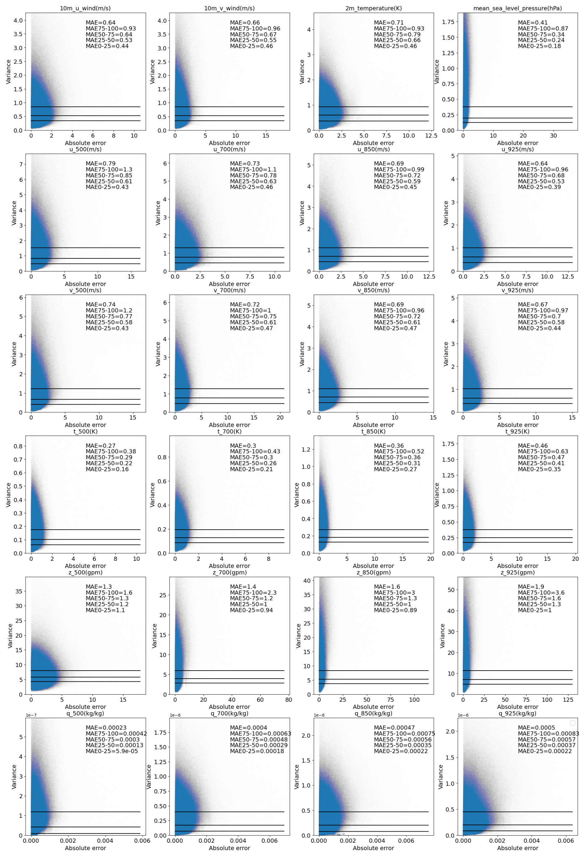
Figure 8 Correlation between the absolute error of Regression 4 and the variance of 20-member CorrDiff 4 predictions for the data from 1 October 2023 00:00 UTC. Each point in the figure corresponds to a grid point. The three black lines in each subplot represent the 75th, 50th and 25th percentile of the variance. These three lines separate the grid points into four groups. MAE75-100 is the MAE of the grid points above the 75th line, MAE50-75 is the MAE of the grid points between the 50th and 75th line, etc.

Figure 9 Illustration of the four uncertainty groups of grid points in Fig. 8. Brighter areas correspond to higher variance.

The spatial distribution of these four uncertainty groups is illustrated in Fig. 9, where brighter areas represent higher variance. These results provide a more intuitive understanding of the predictive uncertainty. For example, the variance of the 2 m temperature over the ocean is significantly lower than that over the land; the variance of the geopotential height over the Qinghai-Tibet Plateau is generally higher than that in other regions; in the bottom row of Fig. 9, the variance in the lower part (which corresponds to areas with more water vapour) of each subplot is higher.

In the CorrDiff framework, predictive uncertainty is estimated using the ensemble variance obtained from multiple stochastic diffusion sampling trajectories. While this approach provides a practical and computationally efficient way to quantify prediction variability, it should be interpreted with care. Specifically, the ensemble variance reflects the sensitivity of the learned conditional generative model to stochastic sampling noise in the denoising process. It does not explicitly correspond to physically grounded quantities such as atmospheric intrinsic predictability, initial condition uncertainty, or model structural error. Therefore, it should not be interpreted as a direct estimate of dynamical forecast uncertainty. We instead interpret the diffusion ensemble variance as an empirical proxy for predictive uncertainty rather than a physically rigorous uncertainty decomposition. Future work will focus on establishing more physically consistent uncertainty quantification frameworks by linking diffusion-based ensembles with atmospheric error growth dynamics and multi-scale predictability theory.

3.3 Downscaling the SFF and CMA-GFS Forecasts

This section applies the trained downscaling models to the low-resolution outputs of the global forecast systems to generate 3 km forecasts. Two global forecast systems are considered: SFF and CMA-GFS. The resulting 3 km forecasts are evaluated against the CMA-MESO model, which serves as our baseline model. The 3 km reanalysis data are used as the ground truth. Notebly, CMA-MESO is driven by CMA-GFS, the latter supplying its initial and lateral boundary conditions. The core assimilation system in CMA-MESO is a three-dimensional variational (3DVar) scheme, which assimilates high-resolution observations.

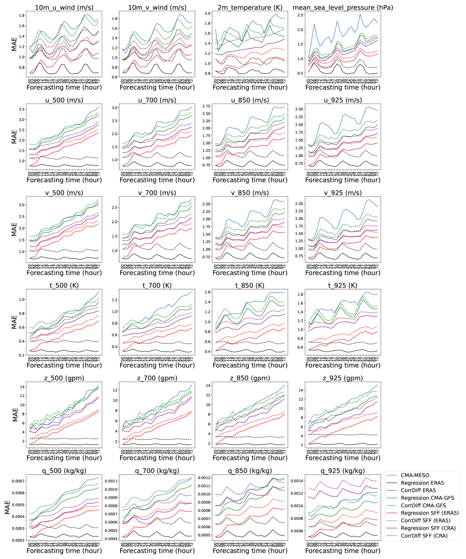
Figure 10 The MAE scores of the 3 km forecasts that include the downscaled SFF forecasts (taking CRA1.5 or ERA5 as initial fields), the downscaled CMA-GFS forecasts and the CMA-MESO forecasts, using the 3 km reanalysis data as the ground truth. The downscaled ERA5 are also present for comparison. The downscaling models are Regression 4 and CorrDiff 4. Seven initialization times are considered: 1 March 2023 00:00 UTC, 1 June 2023 00:00 UTC, 1 September 2023 00:00 UTC, 1 December 2023 00:00 UTC, 24 May 2023 00:00 UTC, 30 July 2023 00:00 UTC, and 4 September 2023 00:00 UTC. The last three times correspond to the periods of Typhoon Mawar, Khanun and Haikui, respectively.

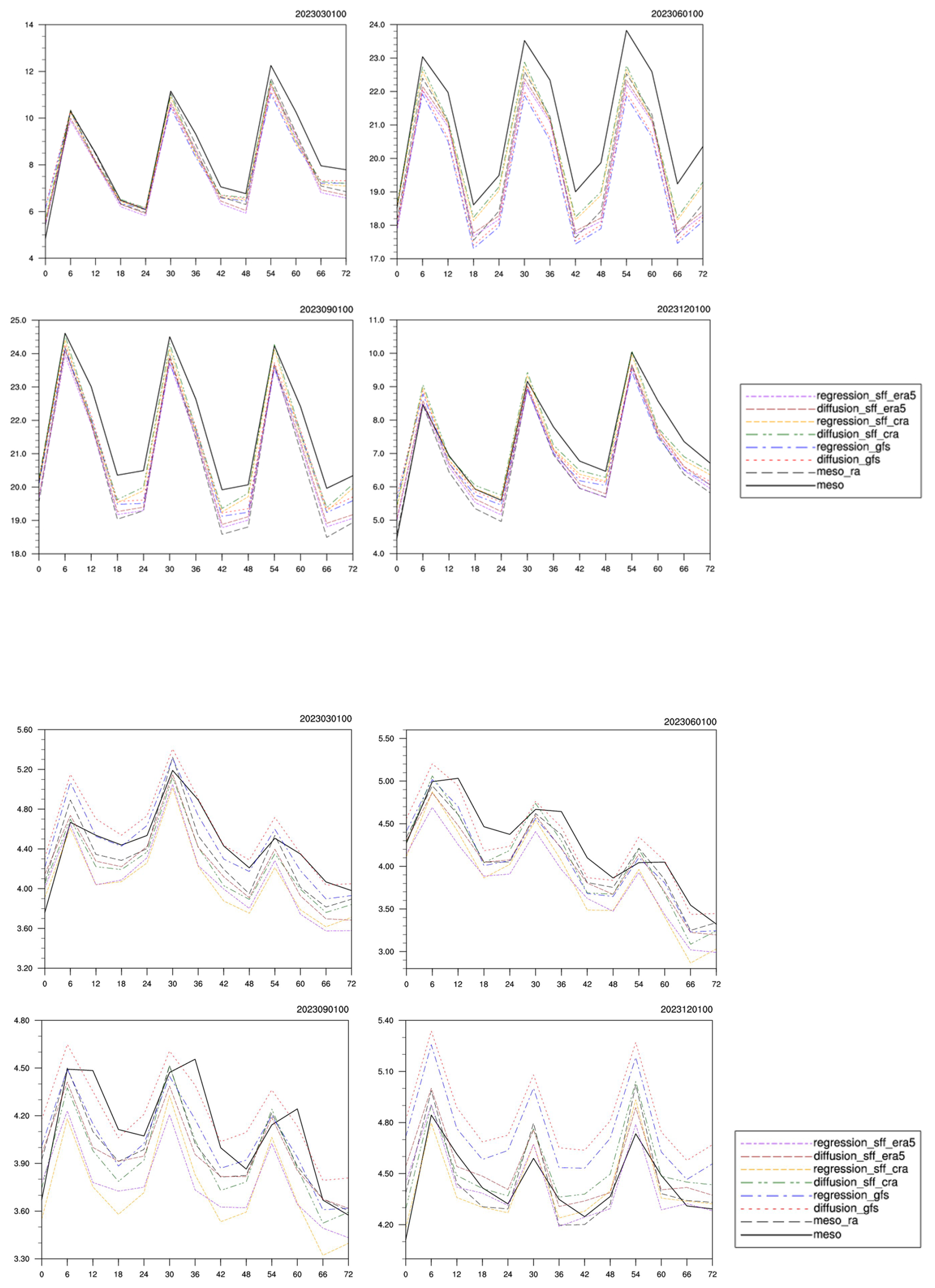
Figure 11 Area average of the 2 m temperature (top) and the 10 m wind (bottom) of the 3 km reanalysis data and the 3 km forecasts of CMA-MESO, downscaled SFF (taking CRA1.5 or ERA5 as initial fields), and downscaled CMA-GFS. Four initialization times are considered: 1 March 2023 00:00 UTC, 1 June 2023 00:00 UTC, 1 September 2023 00:00 UTC, and 1 December 2023 00:00 UTC. “meso_ra” denotes the 3 km reanalysis; “regression” and “diffusion” refer to the Regression 4 and CorrDiff 4, respectively.

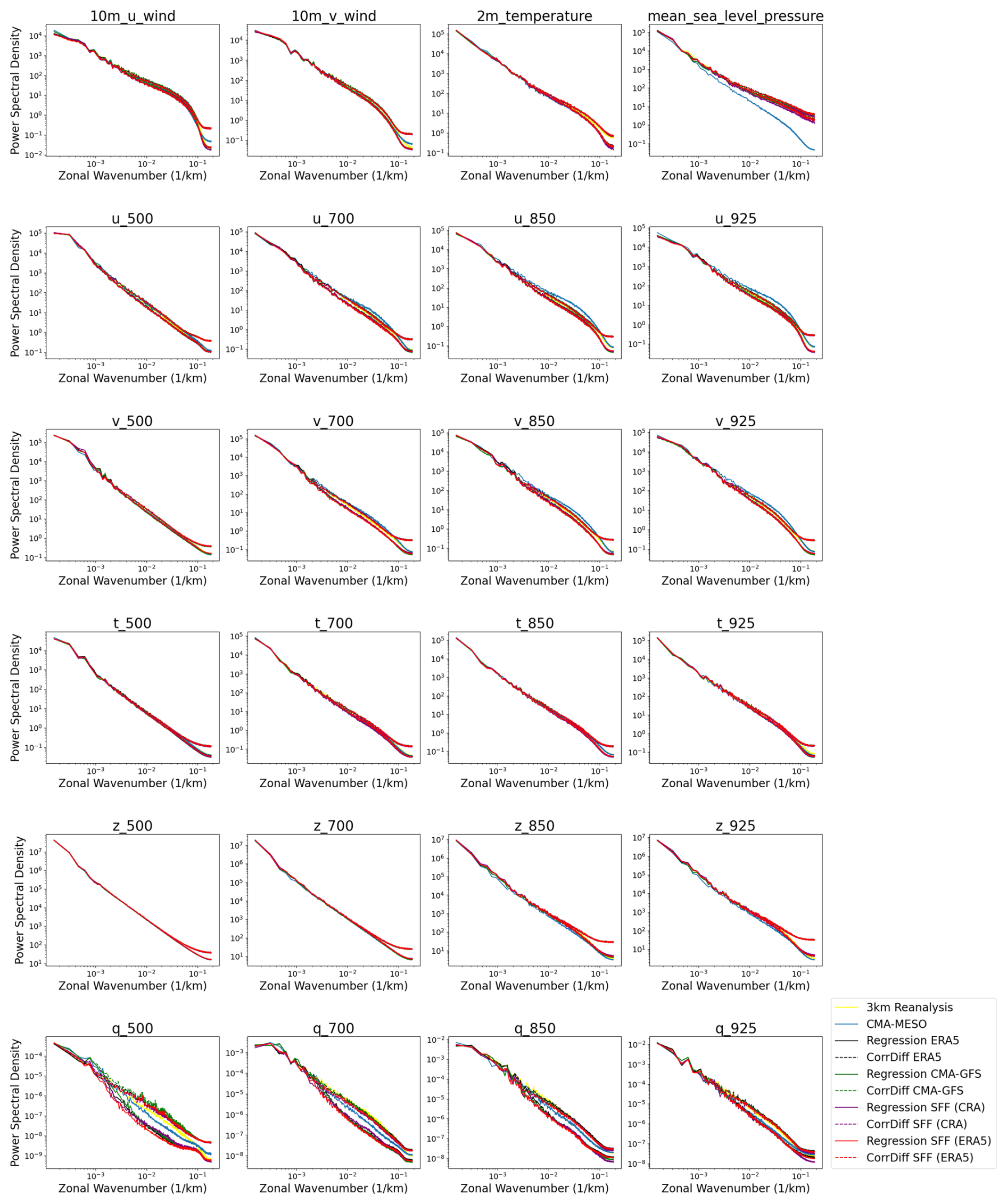
Figure 12 Power spectral density of the downscaling variables. The downscaling models are Regression 4 and CorrDiff 4. The used 3 km reanalysis data and ERA5 are from 2 March 2023 00:00 UTC. The CMA-GFS, CMA-MESO and SFF forecasts are 24 h forecasts that are initialized at 1 March 2023 00:00 UTC.

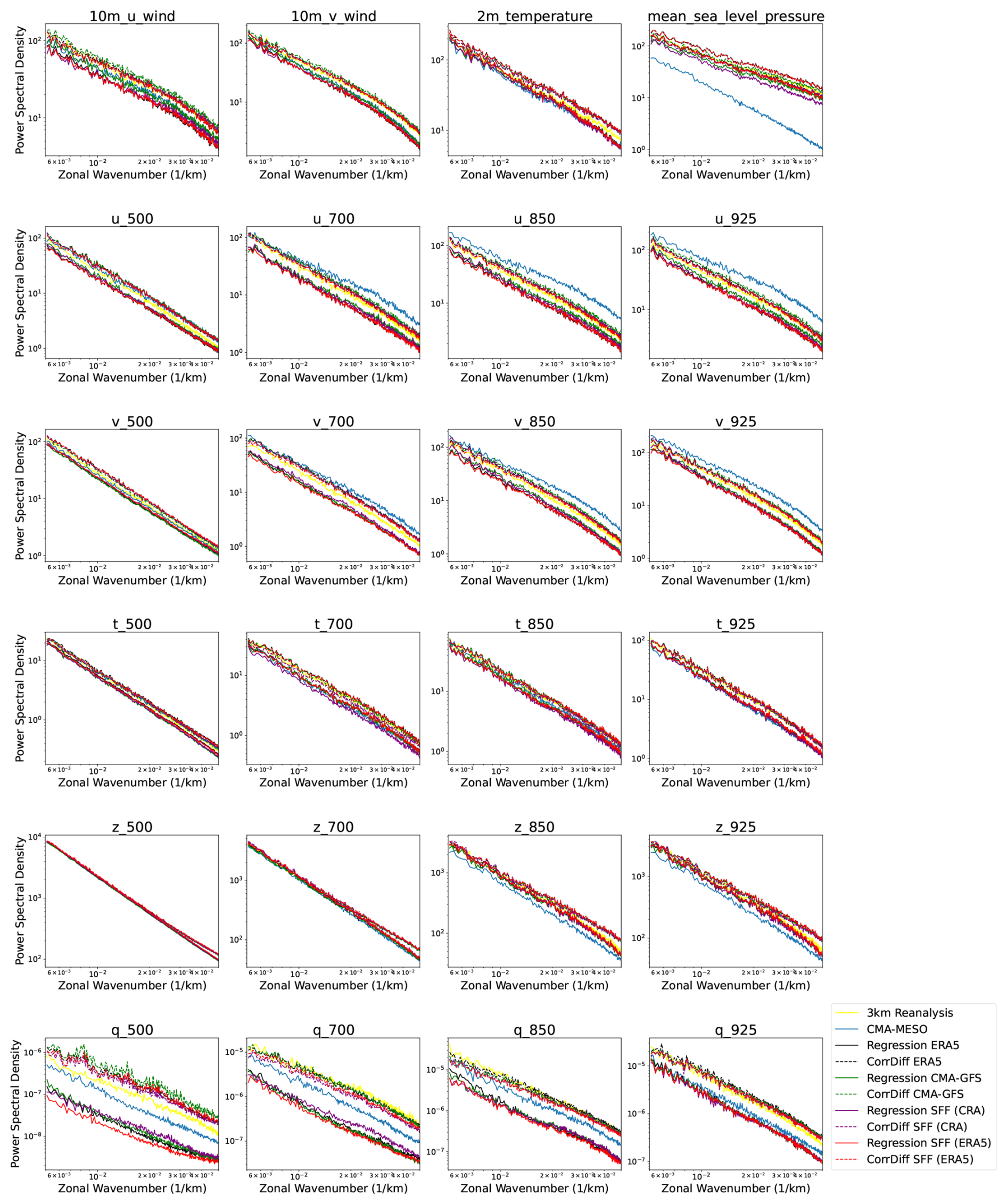
Figure 13 Same as Fig. 12 but showing only the zonal wavenumber interval [0.005, 0.05] to better visualize the details.

3.3.1 SFF

Sphere Fusion Forecast (SFF) is a data-driven deep learning-based weather model developed from Spherical Fourier Neural Operators (Bonev et al., 2023). Compared to Spherical Fourier Neural Operator, two major improvements are made in SFF: the up-sampling and down-sampling operators between the Spherical Fourier Neural Operator blocks are added, allowing the initial and final stages of the Spherical Fourier Neural Operator block chain to handle broader frequency spectra, while the middle layers focus on relatively low-frequency information; a Vision Transformer–like architecture between the encoder and decoder is introduced as the skip connection, which improves the model's capacity for local feature learning, producing more robust and accurate forecasts.

3.3.2 CMA-GFS

China Meteorological Administration-Global Forecast System (CMA-GFS) is a global model developed by the CEMC. It comprises a semi-implicit semi-Lagrangian non-hydrostatic dynamical core, a physical parameterization package, and a four-dimensional variational data assimilation system (Chen et al., 2008). Currently, the horizontal resolution of CMA-GFS is 0.125° × 0.125° (≈ 12.5 km).

3.3.3 3 km Forecast Evaluation

Figure 10 shows the MAE scores for the 3 km forecasts that are based on the 25 km forecasts of different global models. The current operational CMA-MESO provides forecasts up to 72 h, so we also consider 72 h forecasts for comparision. The downscaling results for ERA5 are also given in each subplot, which can be considered as an upper-bound for the downscaling task. For SFF, forecasts are generated from two initial fields: ERA5 and CRA1.5. In fact, the current version of SFF is trained on CRA1.5, which is a reanalysis dataset developed by the CMA and is utilized in the AIM-FDP project. The daily updates of CRA1.5 are available 2 h behind real time. So, the SFF forecasts using CRA1.5 as initial fields can be considered as real-time forecasts.

In each subplot, regression models exhibit lower MAE scores than the corresponding CorrDiff models, which is consistent with the results on the validation set. In all figures, the curves of the downscaled ERA5 (black curves) exhibit the lowest MAE scores, followed by the downscaled SFF forecasts that take ERA5 as initial fields (red curves). For most variables except specific humidity, generally, the downscaled SFF forecasts that uses CRA1.5 as initial fields (purple curves) are better than the downscaled CMA-GFS forecasts (green curves), which in turn are better than the CMA-MESO forecasts (blue curves). In general, these results in Fig. 10 indicate that, in terms of the MAE scores, our data-driven models can potentially outperform CMA-MESO for most variables.

Figure 11 show the area average of the 3 km reanalysis data and 3 km forecasts for the 2 m temperature and 10 m wind. The forecasts of the 2 m temperature are fairly consistent with the 3 km reanalysis data, but there are significant inter-model differences for the 10 m wind. The 10 m wind trend in the 3 km reanalysis data clearly differs from that in the CMA-MESO forecasts. All forecasts based on the downscaling models exhibit trends more closely aligned with the 3 km reanalysis data. Among them, the downscaled CMA-GFS forecasts produce higher wind speeds than the downscaled SFF forecasts. This difference is likely due to the over-smoothing of the outputs of data-driven models like SFF, which reduces intensity.

To comprehensively evaluate the outputs of the downscaling models, we calculate the power spectral density and structural similarity index measure.

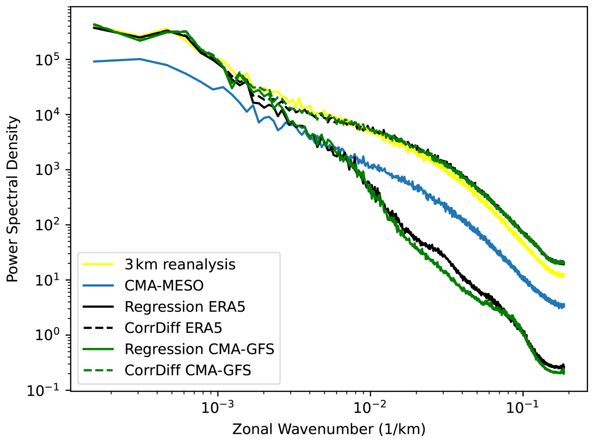
Figure 14 Power spectral density of the radar composite reflectivity. The downscaling models are Regression 2 and CorrDiff 2. The used 3 km reanalysis data and ERA5 are from 31 July 2023 00:00 UTC. The CMA-GFS and CMA-MESO forecasts are 24 h forecasts that are initialized at 30 July 2023 00:00 UTC.

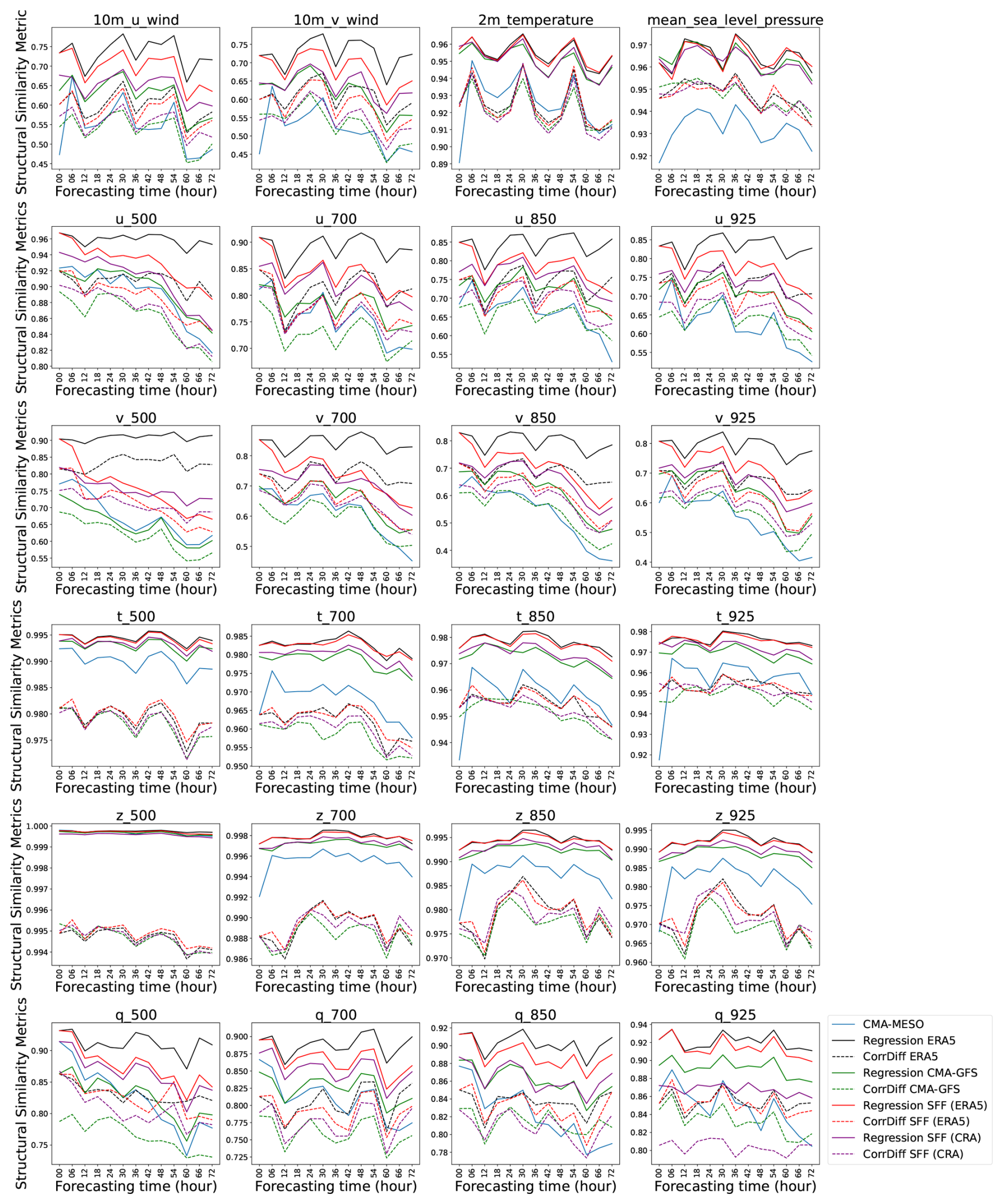
Figure 15 The structural similarity index measure of the 3 km forecasts that include the downscaled SFF forecasts (taking CRA1.5 or ERA5 as initial fields), the downscaled CMA-GFS forecasts and the CMA-MESO forecasts, using the 3 km reanalysis data as the ground truth. The downscaled ERA5 are also present for comparison. The downscaling models are Regression 4 and CorrDiff 4. The initialization time is 1 March 2023 00:00 UTC.

Figure 12 shows the power spectral density of the downscaling variables. In order to improve legibility, a zoomed-in view focusing on the zonal wavenumber range [0.005, 0.05] is provided in Fig. 13. First, the CorrDiff model exhibits higher power spectral density than the regression model, which aligns with the inherent ability of diffusion models to generate richer high frequency details. For most variables, at a zonal wavenumber of approximately 0.2, the power spectral density of CMA-MESO and the regression model is closer to the 3 km reanalysis (which is used as the ground truth) than that of the CorrDiff model, suggesting that CorrDiff may produce some non physical high frequency components. As shown in Fig. 13, the power spectral density derived from the CorrDiff model shows a closer agreement with the ground truth than that from CMA-MESO for most variables, particularly those near the surface, within the zonal wavenumber range of [0.005, 0.05]. For instance, for zonal and meridional wind on 700, 850 and 925 hPa, the power spectral density of the CorrDiff model is significantly closer to the ground truth than that of CMA-MESO and the regression model. Notably, for mean sea level pressure, all downscaling results outperform CMA-MESO. In Fig. 14, for radar composite reflectivity, the CorrDiff model significantly outperforms CMA-MESO in terms of power spectral density, suggesting that diffusion-based models might be well-suited for radar reflectivity prediction.

Figures 15 and 16 illustrate the structural similarity index measure of the downscaled meteorological variables and composite radar reflectivity, respectively. Across all investigated variables, the regression model achieves superior performance relative to CorrDiff. Furthermore, the regression model surpasses CMA-MESO for nearly all variables and all input low-resolution forcing datasets. We further compare three regression-based prediction branches, Regression SFF (ERA5) delivers the best results, followed by Regression SFF (CRA), while Regression CMA-GFS performs the least favorably. This ranking is consistent with the pattern observed in the MAE metrics.

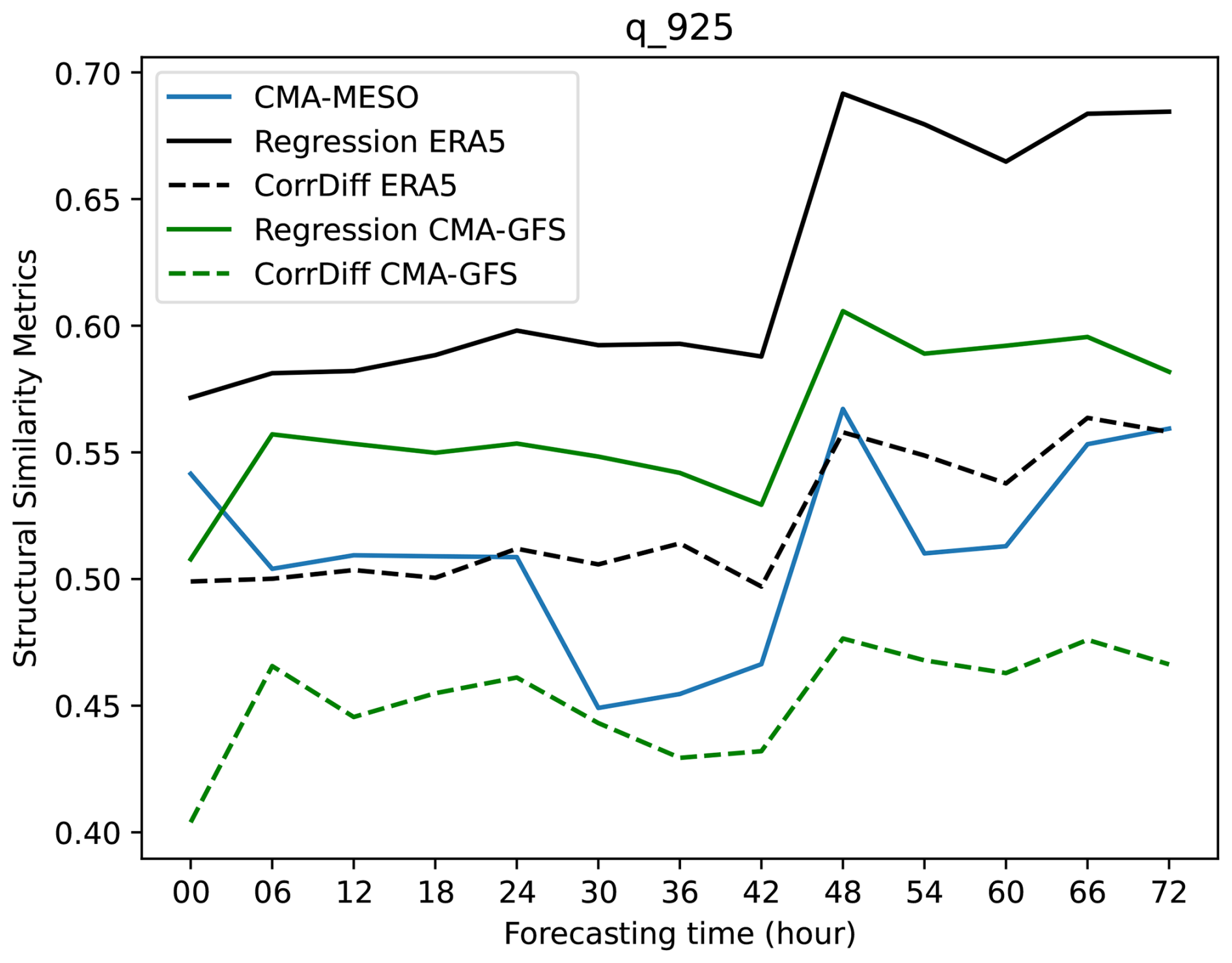
Figure 16 The structural similarity index measure of the 3 km forecasts of radar composite reflectivity that include the downscaled CMA-GFS forecasts, the CMA-MESO forecasts, and the downscaled ERA5, using the 3 km reanalysis data as the ground truth. The downscaling models are Regression 2 and CorrDiff 2. The initialization time is 30 July 2023 00:00 UTC.

3.3.4 Case Study: Tropical Cyclone

Figure 17 shows the 10 m wind speed of the downscaling of Typhoon Khanun by Regression 4 and CorrDiff 4. The downscaling models are applied to the forecasts of CMA-GFS and SFF that use CRA1.5 as initial fields. Generally, the outputs of the regression models are smoother and less sharp than those of CMA-MESO, which should be due to the over-smoothing of data-driven models. Consequently, the Regression SFF forecasts, which involves two data-driven models (SFF and Regression 4), exhibit the most smoothness. The use of diffusion model (CorrDiff 4) notably reduces this effect. Because of the blurriness, the fine-scale structure of the typhoon cannot be clearly captured by data-driven models.

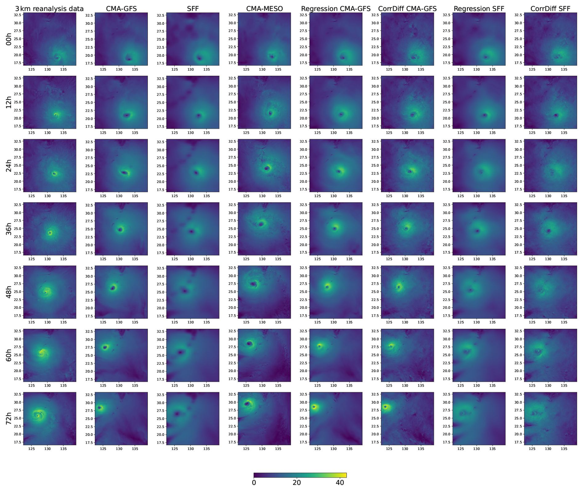
Figure 17 Illustration of the downscaling of CMA-GFS and SFF forecasts of Typhoon Khanun by Regression 4 and CorrDiff 4, compared to the 3 km reanalysis data, CMA-GFS, SFF and CMA-MESO. Figures represent 10 m wind speed. The initialization time is 30 July 2023 00:00 UTC. The initial fields of SFF are CRA1.5.

For the last row in Fig. 17, using the 3 km reanalysis as the ground truth, the MAE scores of CMA-MESO, Regression CMA-GFS, and Regression SFF are 5.24, 4.82, and 2.18 m s⁻¹, respectively. This indicates that a lower MAE does not automatically yield a more realistic visual representation of typhoon winds. Note that the Khanun storm center location of SFF forecasts is closer to that of the 3 km reanalysis data than that of CMA-GFS and CMA-MESO, which should be a reason for the lower MAE scores. In fact, typically data-driven models outperform numerical weather prediction models in the inference of the path of a typhoon, as data-driven models are usually better at predicting large-scale patterns. In order to improve the visual quality of the 10 m wind speed forecasts for typhoons, designing a more sophisticated loss function could be a promising direction. Although, for these results, data-driven downscaling models do not generate visually realistic results of the 10 m wind, their inference of the typhoon eye radius might be better than CMA-MESO, indicating that such data-driven models have the potential to refine the typhoon structure in coarse-resolution forecasts.

Figure 18 Illustration of the 3 km radar composite reflectivity forecasts of Typhoon Khanun by applying Regression 2 and CorrDiff 2 on the CMA-GFS forecasts. The initialization time is 30 July 2023 00:00 UTC.

Figure 18 shows the 3 km radar composite reflectivity forecasts for Typhoon Khanun, obtained by applying Regression 2 and CorrDiff 2 to the CMA-GFS forecasts. The regression model exhibits overly smooth results, failing to predict high radar reflectivity, and it cannot reproduce small reflectivity cores, indicating the limitation of regression models to predict the fine-scale extreme convective precipitation. By contract, the CorrDiff model exhibits a more realistic spatial distribution. The high-frequency features of the CorrDiff model are closer to those of the 3 km reanalysis data, compared to CMA-MESO.

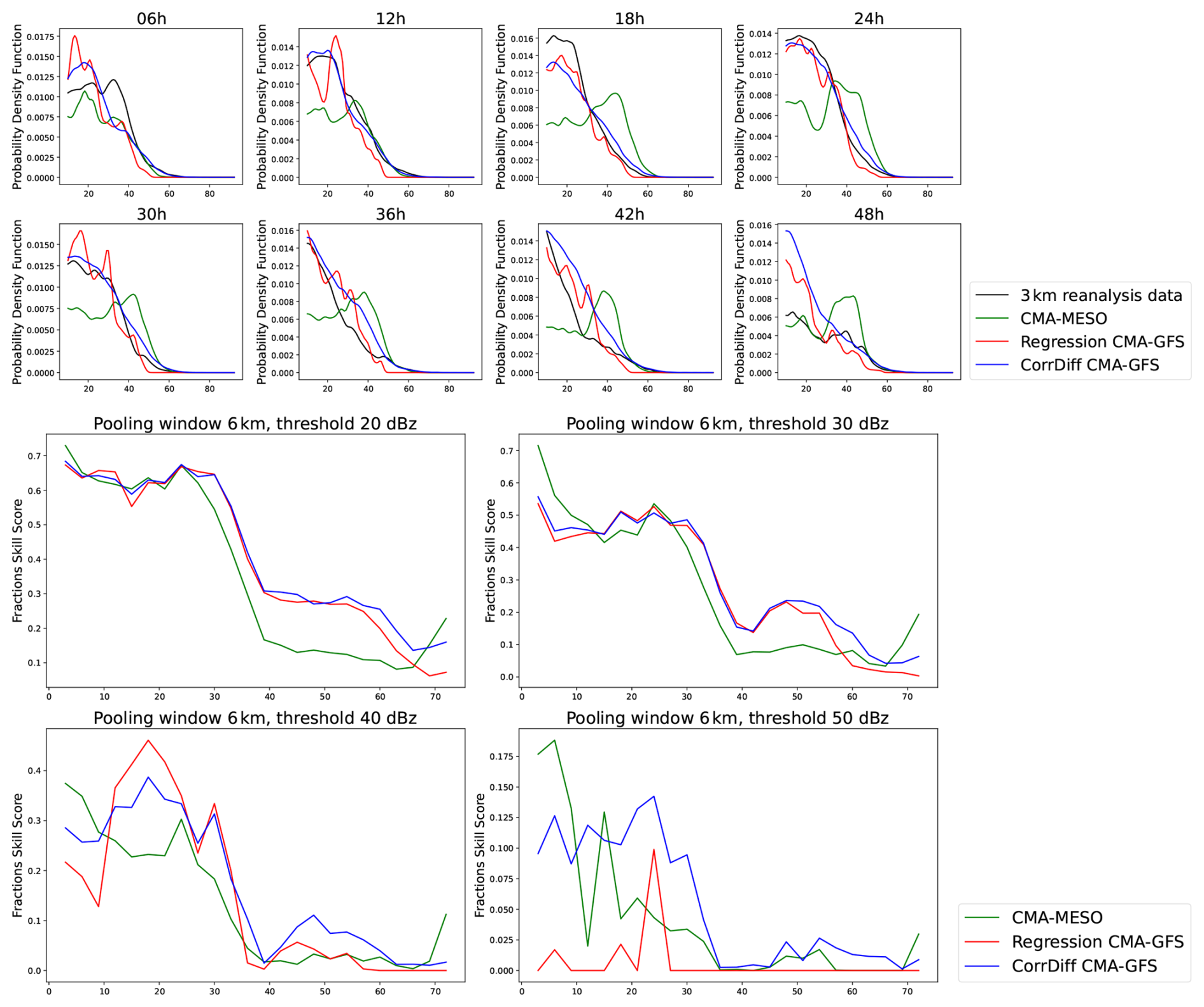
Figure 19 Top: Probability Density Functions of the 3 km radar composite reflectivity forecasts of Typhoon Khanun by applying Regression 2 and CorrDiff 2 on CMA-GFS forecasts, compared with 3 km reanlysis data and CMA-MESO. Only the probability density of the reflectivity that is higher than 10 dBz is shown for clarity. Bottom: Fractions Skill Scores of the 3 km radar composite reflectivity forecasts of Typhoon Khanun by applying Regression 2 and CorrDiff 2 on CMA-GFS forecasts, compared with CMA-MESO, using 3 km reanalysis data as ground truth. The initialization time is 30 July 2023 00:00 UTC.

Figure 19 (top) shows the Probability Density Functions (PDF) for the 3 km radar composite reflectivity forecasts of Typhoon Khanun. Overall, the PDF of the data-driven models aligns more closely with that of the 3 km reanalysis than with that of CMA-MESO. This is particularly evident during the first 24 h for reflectivity exceeding 50 dBZ, where the CorrDiff model (blue curve) more accurately replicates the reanalysis distribution (black curve) compared to CMA-MESO (green curve). For any forecast time, the regression model (red lines) dramatically underestimates the distribution beyond 50 dBz, which is a consequence of over-smoothing, proving that diffusion-based models outperform deterministic models in the prediction of high radar reflectivity or precipitation.

The Fractions Skill Scores for the 3 km radar composite reflectivity forecasts of Typhoon Khanun are given in Fig. 19 (bottom). For all models, there is a dramatic decrease in performance around 36 h. In the first 9 h, CMA-MESO achieves the best Fractions Skill Scores. Between 12 and 36 h, the CorrDiff model can outperform CMA-MESO. CorrDiff and regression models have similar Fractions Skill Score for lower reflectivity thresholds, while CorrDiff substantially outperforms the regression model for high thresholds, since the regression model fails to reproduce high reflectivity.

4 Conclusion

In this work, we train multiple CorrDiff models with different input/output combinations for 3 km downscaling. Evaluation against the CMA-MESO baseline confirms the success of our approach, which generally outperforms CMA-MESO in terms of MAE for the target variables. However, it is important to note that a lower MAE does not necessarily correspond to better forecasts, particularly for extreme weather events such as typhoons. Experimental results also show that, for radar composite reflectivity inference, the CorrDiff model can produce more realistic high-frequency details than the regression model.

One major drawback of our CorrDiff models is that they have higher MAE scores compared to the regression models. This phenomenon was also observed in the original work of CorrDiff. However, in our experiments, the difference in the MAE scores between CorrDiff and regression models is more obvious, which might be due to the fact that the size of our high-resolution grid is much larger than that in the original work. Another limitation is the inference speed of CorrDiff models. Owing to the iterative denoising process, the inference time for a diffusion model is multiple times longer than that of a regression model. This computational overhead increases considerably when generating an ensemble of downscaling results.

Future work could explore several promising directions:

• In current work, only reanalysis data are used to train the models, in order to improve model accuracy, pre-trained models can be further finetuned on operational data. Moreover, they can be finetuned together with SFF.

• Our demonstration of a correlation between the predictive uncertainty quantified by CorrDiff and the MAE enables the future development of methods that use uncertainty estimates to mitigate forecast errors.

• A challenge remains in the interpretability of deep learning models (Zhang et al., 2021). Various methods (for example, gradient-based approaches; Simonyan et al., 2013; Sundararajan et al., 2017) have been developed for computer vision tasks such as image classification. These techniques could be adapted to elucidate the predictions of CorrDiff by incorporating physical principles.

• Distinct prediction patterns across different variables and subdomains are observed in this work. The CorrDiff framework could be optimized via subdomain- and variable-specific customized modeling to adapt to heterogeneous regions.

• The current uncertainty estimate is empirically motivated; future work should aim to establish theoretical connections between diffusion-based uncertainty quantification and atmospheric predictability to improve the physical interpretability of uncertainty estimation.