An ESMValTool-based framework for sanity checks, physical consistency and climate fidelity during model development – ICONEval v1.0

Continuous evaluation and performance monitoring during the development of Earth System Models (ESMs) are essential to identify potential problems early, such as unrealistic behavior of climate-relevant quantities, insufficient skill in reproducing the observed basic climate state, or violations of physical laws. The latter is particularly important for the emerging class of hybrid machine learning (ML) enhanced ESMs, where data-driven components are integrated with physics-based model formulations. ESMs used for projections of future climate continue to increase in complexity and resolution. Efficient and user-friendly tools such as the Earth System Model Evaluation Tool (ESMValTool) can therefore greatly support the assessment of a model. So far, ESMValTool focused primarily on providing a broad collection of community-developed evaluation diagnostics and recipes, allowing users to perform a large variety of rather detailed assessments across different domains. A main application of the tool was the assessment of multiple ESMs, in particular those participating in the coupled model intercomparison project (CMIP). Here, we introduce ICONEval, an open-source evaluation framework using ESMValTool that complements existing capabilities by enabling rapid, reproducible, and physically informed assessments of model performance, also during development. ICONEval provides efficient parallel processing of ESMValTool recipes and can generate HTML summary reports allowing to easily automatize and visualize evaluation and monitoring of performance during model development. The new capabilities are grouped into three complementary categories: (1) sanity checks, (2) physical consistency checks, and (3) climate fidelity diagnostics. The sanity checks assess whether global mean values of climate-relevant variables are within the bounds derived from observational and reanalysis datasets. The physical consistency checks aim to identify potential violations of constraints imposed by fundamental physics such as conservation of total air mass, realistic variability of atmospheric water vapor with temperature or the temperature dependence of the cloud ice fraction. The climate fidelity diagnostics assess important climate variables from different ESM components, i.e. atmosphere, ocean, and land. Here, we demonstrate this extension of the ESMValTool capabilities by applying the new diagnostics to a historical simulation performed with the ICON-XPP model as an illustrative example. The three-step assessment presented here can be efficiently used to compare different model configurations or versions, for example when testing new or updated parameterizations, including hybrid ML-enhanced (MLe) ESMs, also supporting emerging community benchmarking standards such as ClimateBench. While ICONEval is focused on the ICON model, the underlying ESMValTool diagnostics can also be used for different models as long as the model output is following the CMOR (Climate Model Output Rewriter) standard or the model is supported directly by ESMValTool.

1 Introduction

Earth system models (ESMs) in combination with Earth observations are important tools not only to improve our understanding of present-day climate but also to project climate change under different future scenarios, and in turn inform global climate policy developments. For this, climate models have been continuously improved and extended to the complex state-of-the-art ESMs participating in the latest (seventh) phase of the Coupled Model Intercomparison Project (CMIP7) (Dunne et al., 2025). Particularly when changing or extending components of a model, working on model parameterizations or when optimizing a model's configuration including adjustment of only weakly or unconstrained parameters auch as model tuning, model evaluation is an essential element during model development. Model evaluation usually consists of comparing model output with Earth observations, reanalysis data or other suitable datasets such as the output of an ensemble of state-of-the-art models to assess a model's performance for a given diagnostic or metric. This serves as a quality control mechanism as well as guidance for identifying potential further model improvements. As the models grow increasingly complex and use a higher resolution, evaluation tools play a key role in the assessment of model performance by allowing for an efficient, reproducible and yet user-friendly way of analyzing even large sets of data intense simulations, consistent tracking of model changes over time, and objective comparison across different model configurations or versions. One of these tools is the Earth System Model Evaluation Tool (ESMValTool, see Sect. 2.1), an open-source framework that enables rapid evaluation of model performance. ESMValTool so far focused mainly on the evaluation of multiple ESMs participating in CMIP, also allowing the benchmarking of model performance across CMIP phases (Eyring et al., 2021; Bock et al., 2020). During model development, sanity checks, physical consistency checks, and climate fidelity diagnostics of selected essential climate variables are helpful, particularly for assessments of hybrid machine learning (ML) enhanced Earth system models (Eyring et al., 2024b), which replace physical parameterizations with ML for example for convection (Heuer et al., 2026), cloud cover (Grundner et al., 2025) or cloud microphysics (Sarauer et al., 2025). Here, we present ICONEval that focuses on the evaluation of ESMs during model development providing diagnostics that can directly support community benchmarks such as ClimateBench (Watson-Parris et al., 2022). ClimateBench is an open-source machine learning dataset and benchmarking framework to emulate complex Earth system models for different emission scenarios. The new capabilities are grouped into three categories covering the following aspects: (1) sanity checks, (2) physical consistency checks, and (3) climate fidelity diagnostics. The sanity checks can be used to assess the global representation of selected variables in an ESM simulation, such as the temporal evolution of global means, minima, and maxima. The physical consistency checks can be applied to verify that a model's equations, parameterizations, and numerical methods do not violate any known fundamental laws of physics. The climate fidelity diagnostics are used to verify that the observed basic characteristics of the atmosphere, the ocean and the land surface such as geographical distributions, seasonal and diurnal cycles or mean states are represented correctly in a model simulation. ICONEval can be configured to visualize output on an easily accessible website, which facilitates sharing of the evaluation results. In the following, the tools, methods and datasets used are briefly described.

2 Methods and datasets

2.1 ESMValTool

Earth System Model Evaluation Tool (Eyring et al., 2020; Lauer et al., 2020; Righi et al., 2020; Weigel et al., 2021; Schlund et al., 2023; Lauer et al., 2025; Schlund et al., 2025) is an open-source community-developed diagnostics and performance metrics tool for the evaluation and analysis of climate models and Earth System Models (ESMs). ESMValTool allows for a comparison of single or multiple models against predecessor versions and observations. The aim of ESMValTool is to take model evaluation to the next level by facilitating analysis of many different ESM components, providing well-documented source code and scientific background of implemented diagnostics. Traceability and reproducibility of the results are ensured by providing detailed provenance records for all outputs.

ESMValTool is by now a well-established tool that has been used in numerous European projects resulting in more than 60 peer-reviewed publications (e.g., Tebaldi et al., 2021; Meehl et al., 2020; Gier et al., 2020; Bock et al., 2020). The tool has been used in several chapters of the Sixth Assessment Report of the Intergovernmental Panel on Climate Change (IPCC AR6; IPCC, 2021) and has been selected by the CMIP7 Model Benchmarking Task Team as one of the model benchmarking and evaluation tools for the rapid evaluation framework (REF; Hoffman et al., 2026).

The ESMValTool software package provides a large collection of “recipes”, configuration files defining input data, preprocessing steps, and diagnostics to be applied and associated analysis scripts for a large range of scientific analyses. A set of new recipes has recently been added focusing on basic sanity and consistency checks as well as a basic evaluation across the modeling domains atmosphere, ocean and land during model development, e.g. when testing new parameterizations. With this, ESMValTool can now be used to efficiently assess new model runs and check whether a model version under development seems on the right path. Application of these diagnostics as a basis for monitoring a running model simulation is also possible.

2.2 ICON-XPP model

The eXtended Predictions and Projections (XPP) version of the ICOsahedral Nonhydrostatic (ICON) model framework is a coupled Earth system model configuration. An important aim is to provide a model platform for contributions to CMIP7 (Dunne et al., 2025). ICON-XPP includes atmosphere, ocean, land, river, sea ice and interactive carbon components in a fully coupled modeling system. It is designed to bridge numerical weather prediction and climate modeling by using a unified process representation for applications ranging from months to long-term climate projections (Müller et al., 2025).

In order to illustrate ICONEval's new ESMValTool-based capabilities presented in this paper, we use one of ICON-XPP's “historical” simulations performed within the CMIP Diagnostic, Evaluation and Characterization of Klima (DECK) model experiment setup that is often used for improving and comparing coupled Earth system models (Eyring et al., 2016). The historical experiment is driven by historical forcing from CMIP7 and is used to analyze the present-day evolution of climate. The atmospheric component of the ICON-XPP simulation used here has a horizontal resolution of approximately 80 km (R2B5) and 130 vertical levels (L130), the ocean model is run at a resolution of about 20 km (R2B7) with 72 vertical levels (L72). The configuration of the ICON-XPP model used in this historical experiment is an improved version of Müller et al. (2025). Improvement was done in the model physics as well as model parameter tuning in preparation for CMIP7 experiments.

2.3 ICON model evaluation with ICONEval

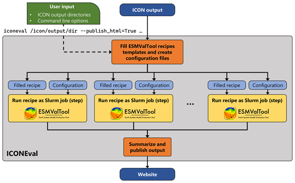
Here, we present ICONEval, an open-source evaluation framework initially tailored to the evaluation of the ICON Earth system model (see Sect. 2.2) and its ML-enhanced configurations during the development phase. Initially, we focus on ICON-XPP, a model that will contribute to CMIP7 and is used in operational climate prediction (Müller et al., 2025), with an active development history. For example, several data driven approaches for ICON-XPP aiming at improving selected parameterizations with machine-learning based methods are being developed such as radiation (Hafner et al., 2026), convection (Heuer et al., 2026), cloud cover (Grundner et al., 2025), gravity waves (Haslauer et al., 2026) or cloud microphysics (Sarauer et al., 2025). Such model development activities require continuous performance monitoring and basic evaluation including sanity checks and physical consistency checks already during the development phase to identify potential problems early on. Particularly during the often-needed retuning of the model when replacing a core parameterization, an efficient and easy-to-use tool is needed that also allows for checking a larger number of model simulations. This gap is filled by ICONEval, which allows to run a whole suite of diagnostics with a single command line enabling automatic testing e.g. right after a simulation is finished. In order to maximize the user-friendliness, the results are then also visualized. ICONEval provides for this easy to read overview pages linking to the individual results accessible via a simple web browser. As a demonstration, ICONEval has been integrated into the HPC environment at the Deutsches Klimarechenzentrum (DKRZ), which uses the widespread Simple Linux Utility for Resource Management (Slurm) for managing jobs and a Swift Object Storage that can be used to make the output of ICONEval easily accessible also from outside the HPC environment. ICONEval is a wrapper around ESMValTool that allows running a set of evaluation tasks on one or more given ICON simulations with a single command line call. For this, ICONEval fills ESMValTool recipe templates with the necessary information on the model simulations, runs these recipes in parallel as Slurm jobs or job steps if already run within a parent job, and creates a summary HTML file to conveniently visualize the evaluation results in a web browser. Optionally, these results can be published to an available web server for easy access also from outside of the HPC environment or for sharing the results. While all diagnostics presented in this paper can in principle also be done with the latest ESMValTool version, the task of developing a model requires an efficient and easy-to-use approach to quickly assess also a large number of simulations. For this, ICONEval provides a ready-made suite of diagnostics that we found useful during model development including model tuning. ICONEval is specifically tailored towards basic automated testing and performance assessment of ICON simulations including a user-friendly visualization of the results. The workflow of ICONEval is schematically shown in Fig. 1. ICONEval provides an extensive set of predefined evaluation tasks that consist of the diagnostics presented in this study, but also contain additional ones as well as detailed comparisons to other state-of-the-art Earth system models such as the CMIP6 models to the diagnostics described by Lauer et al. (2025).

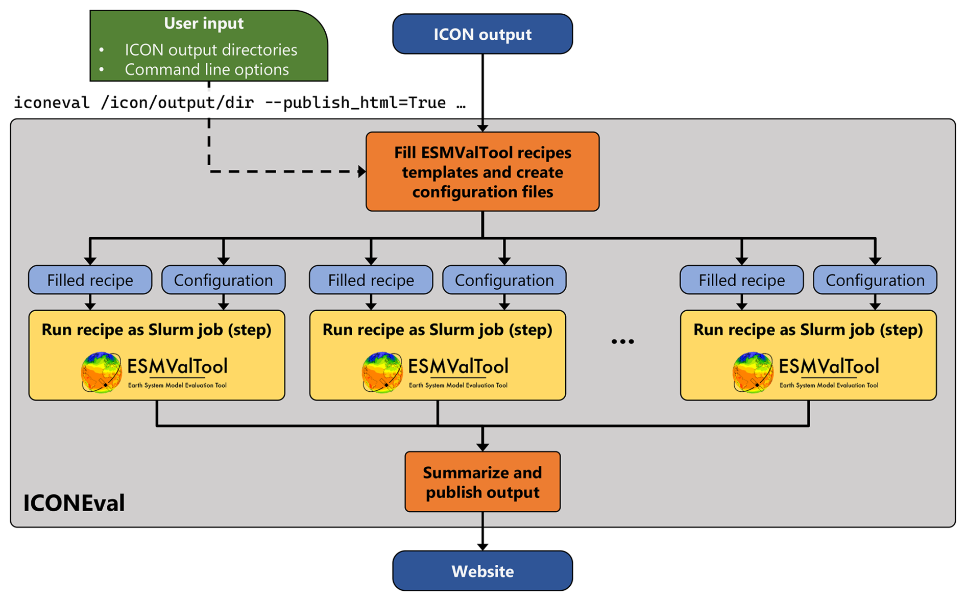
Figure 1 Schematic overview of ICONEval. Based on ICON output from one or multiple simulations, ICONEval fills ESMValTool recipes and creates corresponding configuration files. These recipes are run in parallel by ESMValTool using Slurm job (steps). Finally, results are summarized and if desired published to a website for easy access.

2.4 Datasets

Table 1 provides an overview of all datasets used as reference datasets for the basic model evaluation, sanity checks and consistency checks of model simulations including the variables used and main references for the datasets.

NASA/LARC/SD/ASDC (2018)NASA/LARC/SD/ASDC (2022)Loeb et al. (2009, 2012)Karlsson et al. (2017, 2020)Stephens et al. (2002, 2018)Schröder et al. (2023)Good et al. (2013)Hersbach et al. (2020)Dee et al. (2011)Stengel et al. (2020)Harper et al. (2023)Embury et al. (2024)Adler et al. (2018)Morice et al. (2021)Rayner et al. (2003)Cheng et al. (2024)Rossow et al. (2016)Young et al. (2018)Kobayashi et al. (2015)Zhu et al. (2013)Elsaesser et al. (2017)Gelaro et al. (2017)Platnick et al. (2003)Jung et al. (2011)Compo et al. (2011)Zuo et al. (2019)OSI SAF (2022)Heidinger et al. (2014)Moat et al. (2026)Praveen Kumar et al. (2012, 2013)Boyer et al. (2018)

Table 1 Overview of the reference datasets used for the climate fidelity diagnostics as well as the consistency and sanity checks implemented in ESMValTool in alphabetical order.

3 Sanity checks

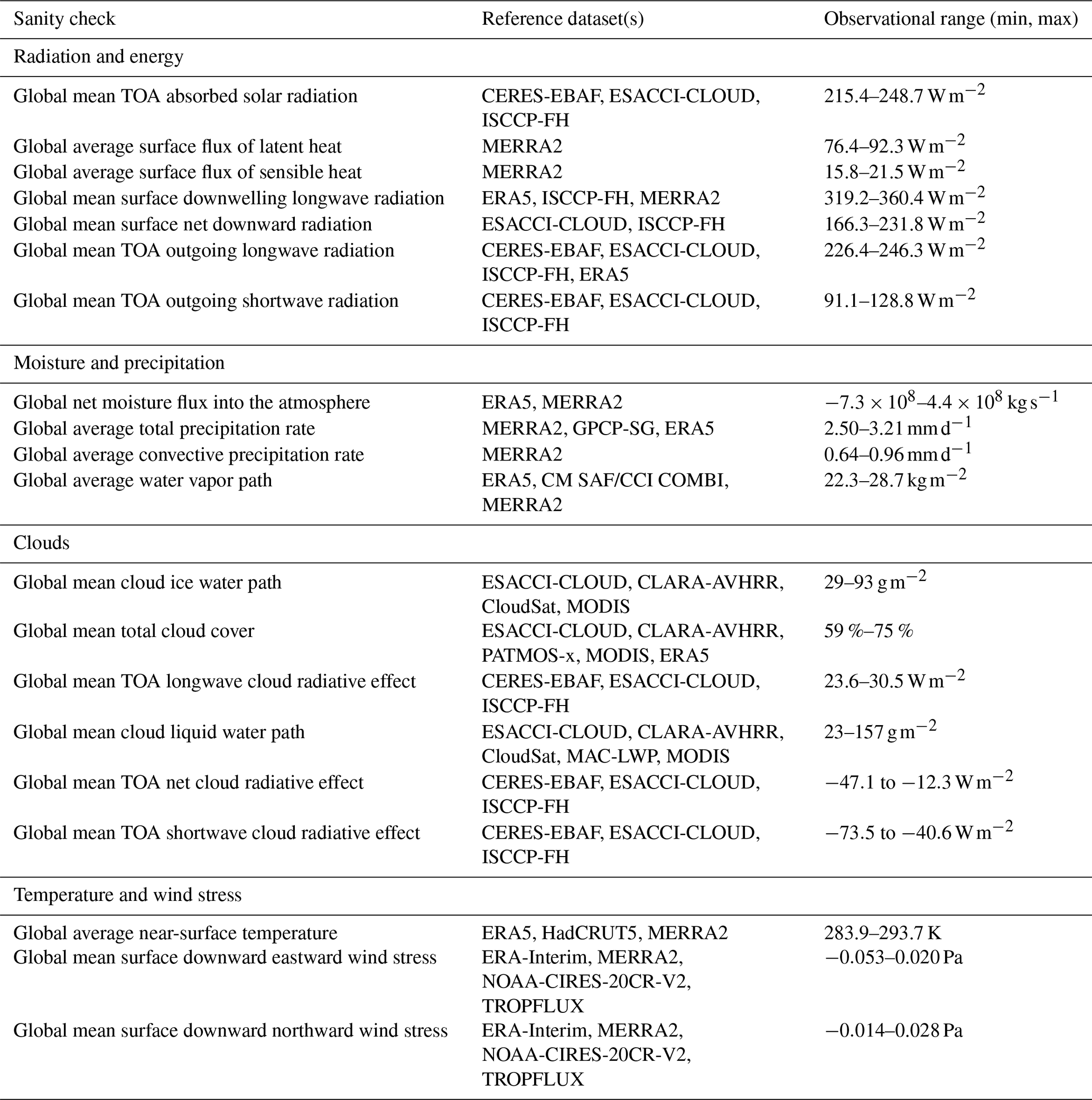
With sanity checks, the global representation of selected variables in an ESM simulation, such as the temporal evolution of global means, minima, and maxima can be assessed. “Reasonable” upper and lower limits for global means are defined using the global minimum and maximum monthly values across all available years of multiple observational and reanalysis datasets. Consequently, these limits are only meaningful for a climate that is similar to the one described by the observations, roughly from the 1980s to now. The sanity checks cover the following categories: radiation and energy, moisture and precipitation, clouds, and temperature and wind stress. As illustrated in the example Fig. 2, the sanity plots display the model output time series in blue (solid line) alongside the observational range in red, marking the observed minimum and maximum monthly mean values of the corresponding variable. These bounds are precomputed for runtime efficiency, with the references listed in Table 2. The diagnostic also displays the minimum and maximum monthly mean values across all model grid cells as dashed lines. This allows for checking that a variable is within physically reasonable limits at all grid cells, e.g. for the variable “total cloud cover” between 0 % and 100 %. Values falling outside these observational and physically reasonable bounds indicate that the simulation should be re-examined.

In the following, the sanity checks summarized in Table 2 are briefly introduced by category.

Table 2 Overview of the sanity checks implemented in ESMValTool.

3.1 Radiation and energy

Radiation and energy fluxes are the core processes that ensure the model is built on sound physical principles and can accurately simulate the Earth's climate system. Climate models include representations of physical processes, such as how radiation interacts with gases, clouds, aerosols, and surfaces. Checking fluxes tells us if those representations are accurate. The energy budget of an ESM must roughly balance incoming solar radiation with outgoing longwave radiation plus storage in the Earth system. Significant deviations could indicate errors in radiative transfer or missing feedbacks such as, for instance, e.g. cloud albedo and would require further investigation. Demonstrating that the model accurately simulates energy fluxes is essential to building confidence in its ability to predict future climate changes (Wild, 2020). Satellite instruments provide global measurements of radiation fluxes at the top of the atmosphere (TOA) and at the surface. Here, these are the primary benchmarks for model evaluation.

We included the TOA absorbed solar, longwave (see Fig. 2), shortwave and net radiation, the surface downwelling longwave radiation and the latent and sensible heat flux in the set of variables for the sanity checks regarding radiation and energy (see Table 2).

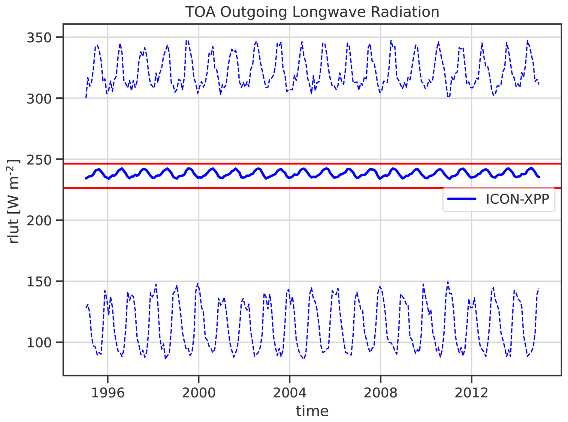
Figure 2 Time series of global monthly mean (solid line) and minimum/maximum across all grid cells (dashed lines) TOA outgoing longwave radiation. Red horizontal lines show “reasonable” upper and lower limits for the global mean calculated from minimum and maximum global monthly mean values found in reference datasets, i.e. observations, reanalyses across all months and all reference datasets.

3.2 Moisture and precipitation

Checking the global moisture flux, precipitation rates (total and convective), and water vapor path (see Table 2) are critical for validating climate models. These metrics are the basis for checking that the model accurately conserves water and energy, fundamental requirements for a realistic simulation of the Earth system. Discrepancies reveal issues with how the model handles evaporation, cloud formation, convection, or atmospheric moisture transport. By comparing model outputs to satellite and other observational data, these processes can be refined if needed, building confidence in the model's ability to predict future climate changes and hydrological patterns.

3.3 Clouds

Clouds play an essential role in climate as key components in the hydrological cycle and by reflecting substantial amounts of incoming solar radiation and by absorbing outgoing longwave radiation, the so-called cloud radiative effect (cre). A basic set of cloud variables is therefore also included in the sanity checks. Key variables investigated here include global mean cloud ice and liquid water paths, total cloud cover, and the TOA radiative effects in both, shortwave and longwave spectra (see Table 2). These checks assess how accurately the model simulates basic cloud properties – their amount, cloud phase (liquid/ice), and their impact on the Earth's energy balance. Comparing modeled values with satellite observations checks whether the model correctly captures the clouds' role in reflecting incoming solar radiation, trapping outgoing infrared radiation, and ultimately determining the net radiative forcing exerted by clouds. Simulating realistic clouds is a crucial prerequisite for trustworthy climate models, as clouds remain a significant source of uncertainty in climate projections and strongly influence global temperatures and precipitation patterns. As the uncertainties in observational datasets of cloud properties are typically large, it is important to include different observations to display a possible range.

3.4 Temperature and wind stress

Near-surface temperature validation can be used as a proxy for a model's energy balance and its representation of key processes like greenhouse gas effects and land-atmosphere interactions. Simultaneously, monitoring surface wind stress can be used to assess a model's representation of the atmospheric forcing on ocean currents and large-scale circulation patterns like the trade winds. Accurate representation of both, temperature and wind stress, is essential for simulating realistic climate states, predicting regional climate variability, and a correct ocean-atmosphere coupling.

4 Physical consistency checks

ESMs are built on known fundamental laws of physics. Physical consistency checks ensure that the model's equations, parameterizations, and numerical methods correctly represent these laws. This is of importance as simplified representations of subgrid processes such as newly developed data driven parameterizations of convection or cloud microphysics might violate some physical constraints. Complying with basic physical consistency checks can be seen as a necessary even though not sufficient precondition to allow for realistic future projections. The set of different physical consistency checks available in ESMValTool is summarized in Table 3.

The implemented consistency checks summarized in Table 3 are focused on atmospheric parameters and should be seen as a starting point. They can be extended further depending on the focus of the model development efforts. In the following, the available consistency checks for the atmosphere are briefly introduced.

Table 3 Overview of physical consistency checks, focused on atmospheric parameters, implemented in ESMValTool.

4.1 Mass conservation

The mass of air is usually treated as a conserved quantity in climate models, i.e. the total mass of air should remain constant during a climate model simulation (Trenberth and Smith, 2005). A violation of this rule would lead to an increase or decrease in the global average surface pressure, which is used as a proxy for the total mass of air. Here, this mass conservation is checked by calculating the anomalies of the surface pressure (p_s) integrated over the whole surface area of the globe. In order to obtain easier to read numbers, the anomalies are calculated as relative anomalies using the whole time period as reference period. Ideally, these anomalies in total air mass should remain close to 0 %. The reanalysis datasets investigated as a reference (ERA5 and MERRA2) show maximum fluctuations of about 0.02 %.

The amount of water vapor in the atmosphere is highly variable in space and time (Trenberth et al., 2007) but the global total mass of water vapor remains approximately balanced through evaporation and precipitation. A time series of the total amount of water vapor in the atmosphere, here calculated as the global sum of the vertically integrated amount of water vapor per unit area (water vapor path), is therefore expected to show only small variations in its amplitude throughout a year.

4.2 Temperature dependence of water vapor

The amount of atmospheric water vapor depends strongly on temperature. This fact can be used to formulate an empirical annual mean temperature-moisture relationship over a selected time period. If the relative humidity in the lower troposphere stays roughly constant, the total column water vapor (prw) would be expected to increase by about 6 %–7 % per degree of warming (Boer, 1993). As proxies for the amount of atmospheric water vapor, we use the global mean water vapor path and for temperature the global mean 2 m temperature (T_2 m). Wan et al. (2024) showed that while the relationship between total precipitable water and T_2 m does not necessarily scale on regional scale with the Clausius-Clapeyron equation describing how the saturation vapor pressure of water changes with temperature, it aligns with the equation in the 15–55° N latitude band (6 %–8 % per degree warming). Here, we calculate anomalies in global annual average T_2 m and prw for each year. Similar to Wan et al. (2024), we use a time period starting in 1993 for the analysis but end in 2014, which is the last year available from the ICON-XPP example simulation. The anomalies are calculated using the whole 22-year period as reference period. In contrast to Wan et al. (2024), we do not calculate separate trends for T_2 m and prw, but calculate the slope of a regression line with x=ΔT_2 m (in K) and y=Δprw (in %). This approach is simple yet robust enough for a consistency check of the relation between temperature and water vapor on global scale. We would like to note that the actual values depend on the time period analyzed. Similar to Wan et al. (2024) we find higher values in the more recent time period 1993–2021 compared with the maximum time period available for the reanalysis datasets investigated (ERA5, JRA-55, MERRA2). An example of this diagnostic is shown in Fig. 3 comparing results from ERA5 with the ICON-XPP simulation over the time period 1993–2014.

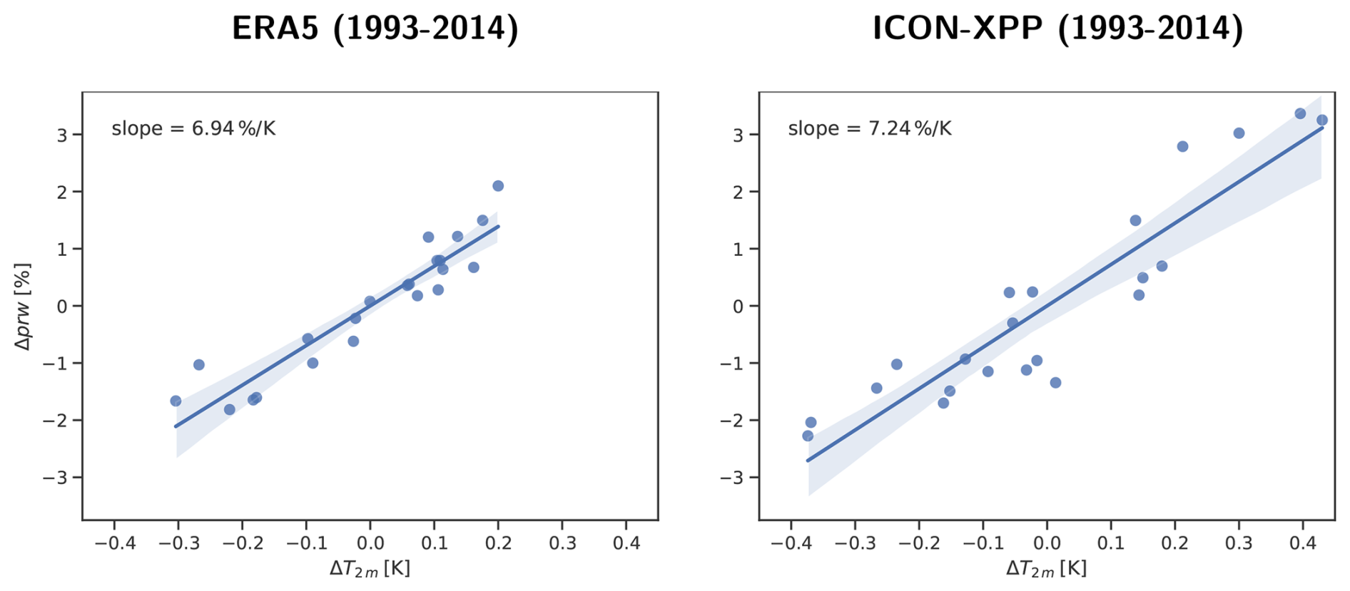
Figure 3 Linear correlation of global annual mean anomalies in 2 m temperature (ΔT_2 m, x axis) and relative global annual mean anomalies in water vapor columns (Δprw, y axis). Left: ERA5, right: ICON-XPP over the time period 1993–2014.

4.3 Cloud ice fraction

The fraction of cloud water that is frozen particularly depends on temperature. Typically, the cloud ice fraction reaches about 100 % at the threshold temperature for homogeneous freezing at roughly −38 °C (e.g. Atkinson et al., 2016) resulting in pure ice clouds. Above the melting temperature of 0 °C, all remaining cloud ice particles begin to melt resulting in pure liquid water clouds, i.e. the cloud ice fraction is approaching zero. In between these two threshold temperatures, typically mixed-phase clouds exist with an ice fraction increasing steadily between 0 % at 0 °C and 100 % at −38 °C. This consistency diagnostic allows to check whether a model can reproduce the qualitative relationship between temperature and cloud ice fraction obtained from vertically resolved measurements or measurement-based data of cloud ice (CALIPSO-ICECLOUD), cloud liquid water content (CLOUDSAT-L2) and temperature (ERA5). We would like to point out, that we are using monthly means resulting in a blurring of the ice fraction and leading e.g. to the possibility of small ice fractions even above 0 °C. Retrieval of the vertically resolved cloud ice and cloud liquid water content from space is subject to large uncertainties. For example, a clear distinction between cloud particles and precipitation is challenging (e.g. Waliser et al., 2009) and the instruments can show saturation effects or a limited sensitivity to certain cloud types (e.g. Marchand et al., 2008). The shape of the cloud ice fraction from observations is therefore only used for a qualitative comparison with the model data. For the calculation of the average cloud ice fraction–temperature relationship, all 3D grid cells are used and binned into 20 temperature bins. Grid cells with a cloud water mass concentration below 10⁻⁶ kg kg⁻¹ (sum of liquid + ice) are not taken into account. Figure 4 shows an example of the cloud ice fraction from ICON-XPP compared with the reference datasets CALIPSO-ICECLOUD, CLOUDSAT-L2, ERA5.

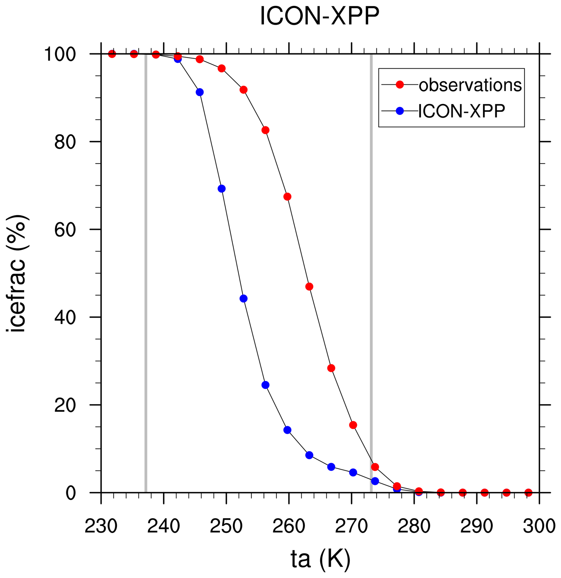
Figure 4 Global average fraction of the cloud ice water content (in %) calculated from monthly means of 3D cloud ice and cloud liquid water content over one year (2014) binned by air temperature. The ICON-XPP model is shown as blue dots, the reference line from the combined datasets of CLOUDSAT-L2, CALIPSO-ICECLOUD and ERA5 in red. The gray vertical lines illustrate the temperatures of homogeneous freezing (−38 °C) and the melting temperature of ice (0 °C).

4.4 Tropospheric lapse rates

The lapse rate is defined as the vertical temperature gradient $\mathrm{\Gamma }=-\frac{\mathrm{d}T}{\mathrm{d}z}$, typically in K km⁻¹ and is a measure for the atmospheric stability. In dry conditions, the lapse rate amounts about 9.8 K km⁻¹, so-called dry adiabatic conditions. The lapse rate depends on the humidity and temperature with warm, humid conditions typically leading to smaller lapse rates than dry cold conditions. On average, lapse rates in the tropical troposphere above the boundary layer are expected to be smaller than in mid- or high-latitudes (e.g. Stone and Carlson, 1979). Here we analyze probability density functions (PDFs) of the 3D tropospheric lapse rates above the boundary layer in the Tropics (30° S–30° N), Northern Hemisphere mid-latitudes (40–60° N) and Southern Hemisphere mid-latitudes (60–40° S) in the altitude range 850 to 250 hPa. For comparability reasons, the model and reference data are interpolated to the same vertical levels (here: 850, 825, 800, 775, 750, 700, 650, 600, 550, 500, 450, 400, 350, 300, 250 hPa). In the example shown in Fig. 5, the peak of the lapse rate PDFs are around 5 K km⁻¹ in the Tropics and 6.5 K km⁻¹ in mid-latitudes.

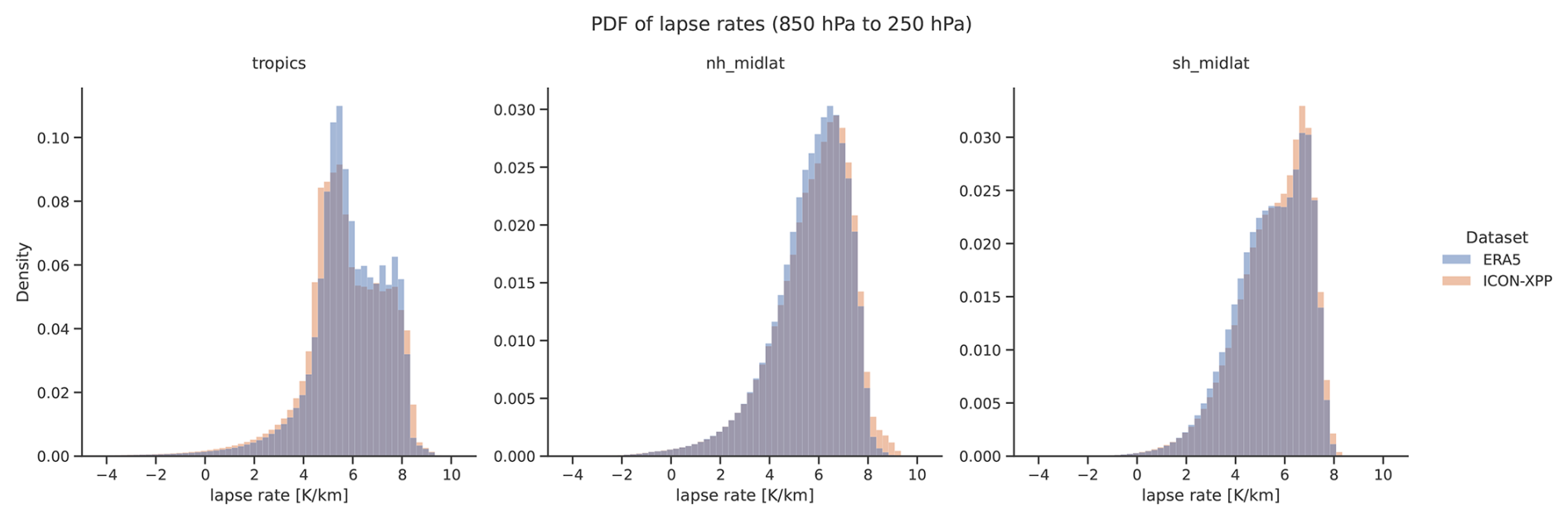
Figure 5 Probability density functions of the 3D lapse rates from ERA5 (blue) and ICON-XPP (orange) in the altitude range 850 to 250 hPa calculated from monthly mean temperatures over the time period 1995–2014. From left to right: Tropics (30° S–30° N), Northern Hemisphere mid-latitudes (40–60° N) and Southern Hemisphere mid-latitudes (60–40° S).

5 Evaluation of climate fidelity

Before new simulations can be used for scientific analyses, it is important to make sure that the basic characteristics of the atmosphere, the ocean and the land surface are represented correctly. This is done by comparing the simulations to observational data records (Hassler et al., 2026) and is therefore only applicable for simulations spanning the most recent decades. We created diagnostics that can be used to evaluate climatologies, annual and diurnal cycles, geographical distributions and time series of different dataset aggregations. The diagnostics are flexible enough to allow their use for many different variables without the need to adjust anything in the code. Due to their relatively simple nature, they solely fall into the “variability and biases” evaluation approach, a classification introduced by Hassler et al. (2026), and do not aim for an in-depth and complex analysis, which requires more specialized and process-oriented diagnostics. However, these simple diagnostics provide an extremely valuable first check of a simulation and a quick assessment of its quality and usefulness. As a particular goal of ICONEval is to accelerate development of hybrid ML-enhanced (MLe) ESMs that focus on reducing systematic model errors (Eyring et al., 2024b, a), we also include precipitation extremes, diurnal precipitation cycle and double-ITCZ (intertropical convergence zone).

Table 4 provides an overview of the climate fidelity diagnostics available sorted by model component, here: atmosphere, ocean, land. These are briefly introduced in the following and can be extended depending on the focus of the model development including new components such as sea ice, land ice, biogeogemistry, etc.

Table 4 Overview of the climate fidelity diagnostics implemented in ESMValTool for first checks during model development.

5.1 Atmosphere

A main evaluation focus for the atmosphere is on parameters that provide general information about the global climate, such as surface temperature, precipitation, radiation, zonal wind speed, and cloud-relevant parameters including water vapor. Most of these variables are of high interest for future climate estimates with their impact on human population, and therefore their magnitude and distribution in historical simulations need to be well understood.

Three different types of analyses for atmospheric variables are available, all with comparisons to different observational datasets: (1) mean geographical distributions (seasonal of annual means), (2) zonal mean (latitude vs. pressure) aggregations for three dimensional variables (seasonal or annual means), and (3) time series of globally averaged variables (see Table 4). The time series provide the option to fit a regression line as an estimate for the trend over the specified time range. These diagnostics were selected since they illustrate some well-known and long-standing biases of climate models, like the double-ITCZ seen in precipitation fields showing as two zonally elongated narrow belts of high precipitation in the Tropics, south and north of the equator, which are present in model simulations but not in observations (Tian and Dong, 2020) or the cold bias close to the tropopause as seen in vertically resolved temperature distributions (e.g. Bock et al., 2020). Both biases can also be seen in the examples shown in Figs. 6 and 9, respectively.

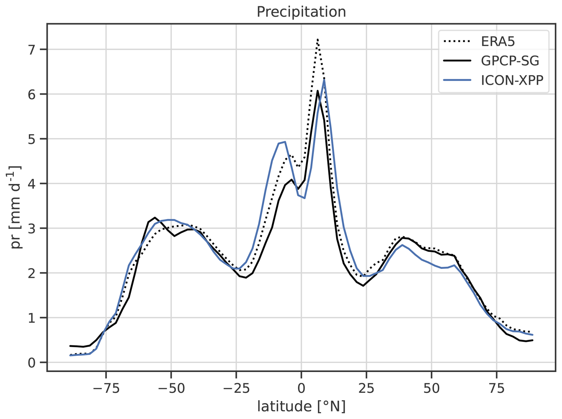
Figure 6 Zonally averaged multi-year annual mean precipitation from ICON-XPP (blue solid line) compared with GPCP-SG (black solid line) and ERA5 (black dotted line).

For precipitation, two additional diagnostics are available to investigate the simulated sub-daily results, (1) the probability density of the precipitation rates at the surface over a specific region (the example shown in Fig. 7 focuses on the Tropics, which are defined here as latitude belt 30° S–30° N) and (2) the hour of daily maximum precipitation rate over a specific region. Here, also an example for the Tropics is shown, Fig. 8.

The histogram shown in Fig. 7 can be used to investigate the frequency of extreme precipitation events. For a fair comparison, both model and reference data (here ERA5) are regridded to the same spatial and temporal grid (here: 1° × 1° and 6-hourly values).

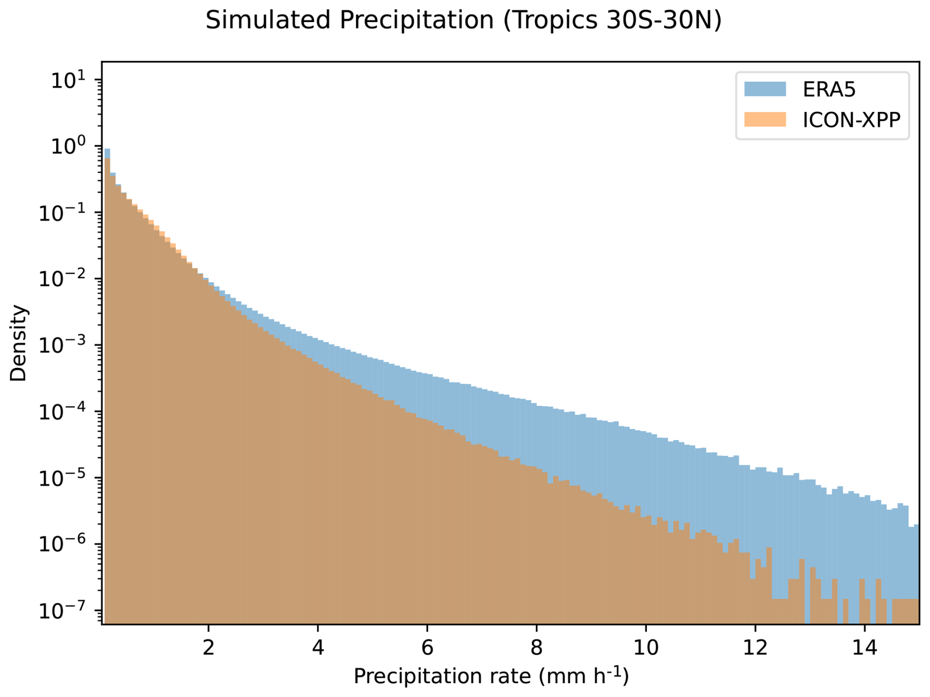
Figure 7 Probability density of the precipitation rates in the Tropics (30° S–30° N) calculated over the time period 2010–2014 from ICON-XPP (orange) compared with ERA5 (blue). All data have been regridded to the same regular 1° × 1° lat-lon grid and averaged to 6-hourly intervals.

The diagnostic calculating the hour of daily maximum precipitation exemplary shown in Fig. 8 can be used to check that basic features of the diurnal cycle such as the land-sea contrast in the timing of the daily precipitation peaks are in agreement with observations. By default, the maximum in the diurnal cycle of precipitation is obtained by applying a discrete Fourier transform (DFT) to the data and using the peak of the first component (MDTF, 2019). Alternatively, a 12 h and a 24 h harmonic fit to the input data can be calculated using the peak of the 24 h harmonic as hour of the daily maximum (Dai, 2024). For this diagnostic, sub-daily model output is required, ideally hourly values. While 3-hourly and 6-hourly output can be used with the diagnostic, the coarse time resolution can result in artifacts such as the vertical stripes that can be seen in Fig. 8. When converting from UTC to local solar time (LST), the temporal frequency of the input data is kept. A location's exact LST will be put into corresponding bins defined by the bounds of the input time coordinate. This means that the lower the time resolution of the input data, the larger the resulting errors that can reach up to time frequency $/$ 2. It is therefore recommended to use this diagnostic with hourly or higher temporal resolution.

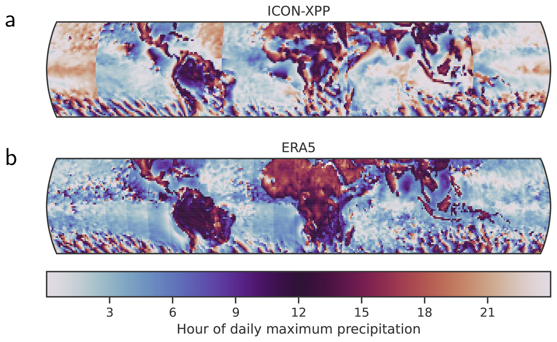
Figure 8 Hour of daily maximum precipitation (local time) in the Tropics (30° S–30° N) for June-July-August calculated over the time period 2010–2014 from (a) ICON-XPP compared with (b) ERA5. The ERA5 data have a time resolution of 1 h, the ICON-XPP of 6 h. A time resolution of less than hourly is not optimal and might introduce some artifacts as can be seen by the striped appearance of the ICON-XPP panel.

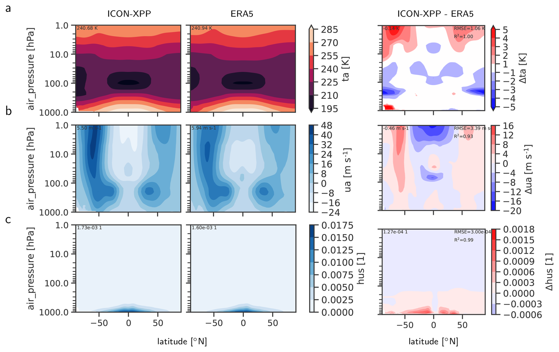
Figure 9 Zonal multi-year annual mean bias in (a) temperature, (b) zonal wind speed, and (c) specific humidity from ICON-XPP compared with ERA5.

5.2 Ocean

Ocean variables of interest can be compared to reanalyses, observations or data from other ESMs. The sea surface temperature is one of the key variables of interest during model development as it determines, amongst other things, the exchange of sensible and latent heat between the ocean and the atmosphere to a large degree. Figure 10 shows the averaged sea surface temperature from ICON-XPP compared with the WOA dataset for the period 1981 to 2010. In the example, the sea surface temperatures from the model and from WOA are in relatively good agreement but biases exist in particular along the western boundary currents, in upwelling regions, in the Southern Ocean and in the North Atlantic Warming Hole (e.g. Kramer et al., 2025) region south of Greenland. ESMValTool includes also diagnostics to evaluate simulated general modes of climate variability like the El Niño–Southern Oscillation (ENSO). Here, we show the time series of the monthly mean sea surface temperature anomalies in the Niño 3.4 region, which is a sanity check of an ESM's ability to represent interannual variability caused by ENSO (Fig. 11). ESMs are not expected to replicate the timing of distinct observed El Niño and La Niña events, nonetheless they should have a comparable amplitude and frequency of the interannual variability in the Niño 3.4 region. The ensemble of CMIP6 models included in this figure provide an envelope for possible anomaly amplitudes that can be expected from current ESMs. As a measure for the strength of the internal variability, the temporal standard deviations of the example model and the reference dataset are given in the top of the panel.

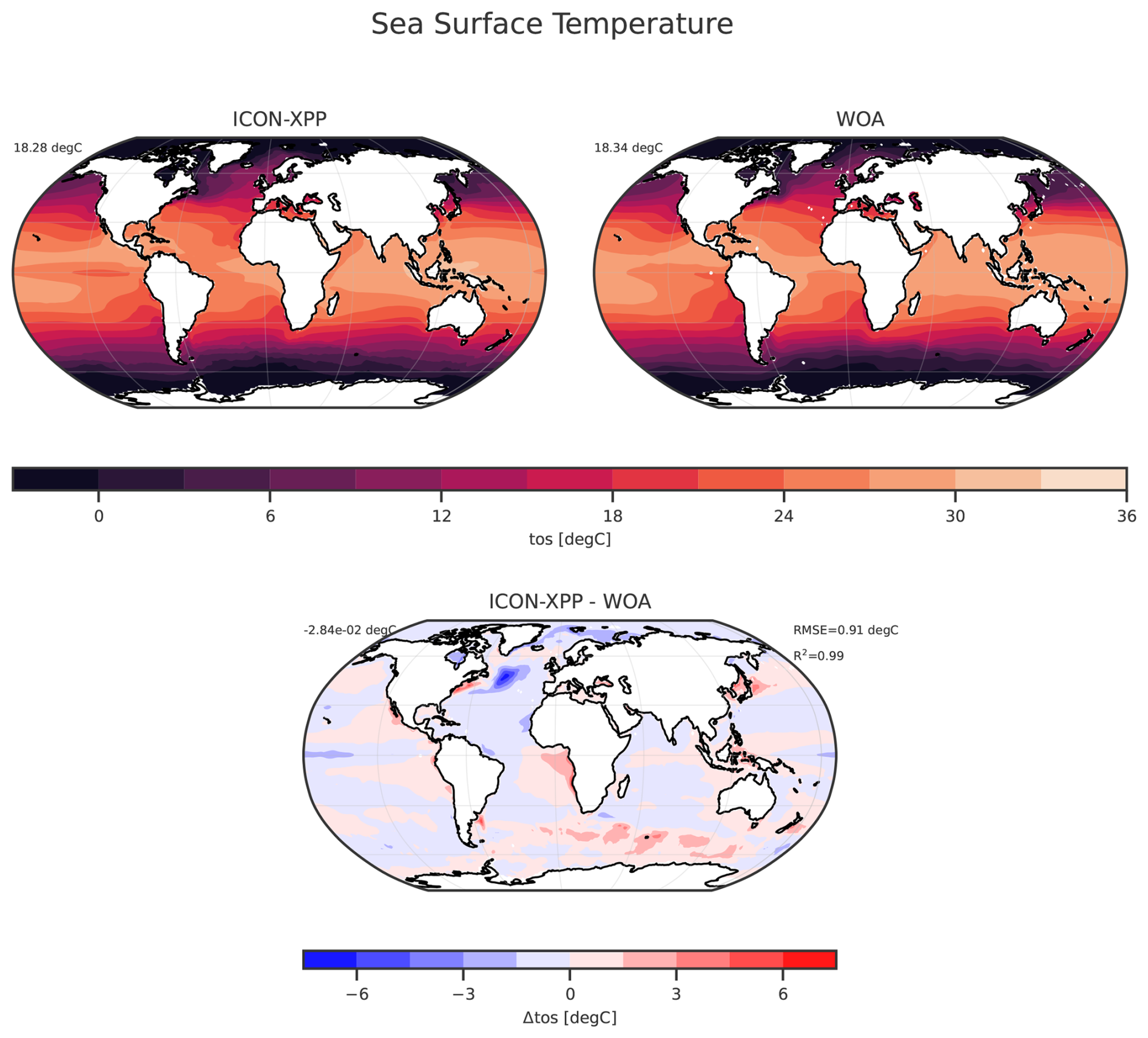
Figure 10 Map plot of the average sea surface temperature for ICON-XPP for the period 1981 to 2010 (left) and WOA for the same time period (right), as well as their difference (below).

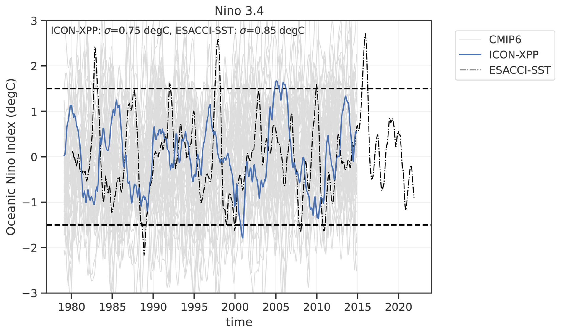
Figure 11 Time series of SST anomalies in the Niño 3.4 region (5° N–5° S and 170–120° W). The black dash-dotted line shows the ESACCI-SST product, the blue line the ICON-XPP results and the thin gray lines results from the CMIP6 model ensemble. The horizontal dashed lines indicate the thresholds of strong El Niño and La Niña events as used by, e.g., the NOAA Climate Prediction Center. The temporal standard deviations (σ) for ESACCI-SST and ICON-XPP are given in the top of the panel. Historical ESM simulations are not expected to replicate the timing of distinct observed ENSO events, but should have a comparable amplitude and frequency of the interannual variability.

Simulating realistic sea ice fields compared to observations is another key aspect during ocean model development. CMIP6 models exhibit pronounced deviations of sea ice area and long-term trends compared to observations especially around Antarctica (Roach et al., 2020), e.g. the Antarctic “sea ice paradox” from the beginning of satellite measurements until 2016. These uncertainties in simulated historical sea ice fields result in low confidence in 21st-century sea ice projections (Fox-Kemper et al., 2021). Recent eddy-permitting simulations indicate some improvement (e.g. Rackow et al., 2022). Thus, sea ice area and extent pose as a suitable target to check the validity of the simulations during model development since they are influenced by e.g. air-sea interactions, ocean and atmospheric circulation and surface albedo. As a proxy for the long-term evolution of sea ice, the sea ice area in the month coinciding with the annual minimum in sea ice area can be used. In the Northern Hemisphere (NH), this is typically in September, in the Southern Hemisphere (SH) in February. Figure 12 shows a time series of the simulated NH and SH sea ice area from ICON-XPP and from the OSI-450 sea ice observational product during the respective months.

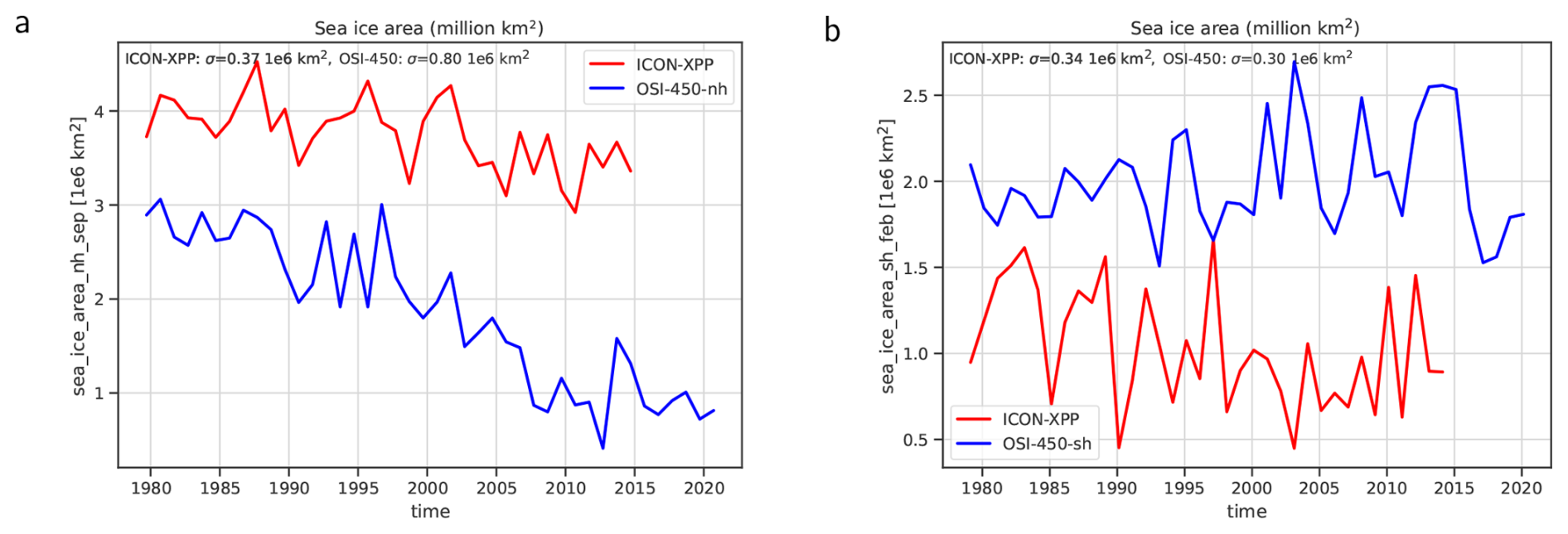
Figure 12 Time series of (a) Northern Hemisphere September and (b) Southern Hemisphere February sea ice area in million km² from ICON-XPP for the period 1979 to 2014 (red) compared with OSI-450 (blue) for the period 1979 to 2020. The temporal standard deviations (σ) for OSI-450 and ICON-XPP are given in the top of the panel. Historical ESM simulations are not expected to replicate the exact timing, but should have a comparable amplitude and frequency of the interannual variability.

Another key metric for the validity of an ocean model during development is the simulated oceanic mixed layer. The mixed layer depth (MLD) determines key processes in the ocean, e.g. deep and mode water formation (Danabasoglu et al., 2014), carbon uptake (Llort et al., 2019) or simulated oxygen minimum zones (Busecke et al., 2022) and is strongly influenced by air-sea interactions. Regions with a pronounced deep water and mode water formation due to a strong seasonal variability of MLD are prone to biases in the simulated MLD compared to observations. These biases are dependent on the ocean models' ability to resolve mesoscale dynamics (Treguier et al., 2023) but also on their sub-mesoscale mixing schemes (Uchida et al., 2026): ESMs often underestimate the MLD in zones with pronounced deep water formation, but also eddy-permitting and eddy-resolving models may exhibit biases due to relying on sub-mesoscale mixing schemes. Thus, the seasonal evolution of MLD in deep and mode water forming regions (see Table 4) is a key metric during ocean model development, e.g. for tuning sub-mesoscale mixing schemes.

Figure 13 shows the mean seasonal cycle of MLD in the Labrador Sea, Southern Ocean, and Weddell Sea in ICON-XPP compared to CMIP6 models and the ORAS5 ocean reanalysis. The maximum MLD is found during winter in Southern and Northern Hemisphere, when deep and mode water masses are formed. In summer the positive surface heat flux in deep and mode water forming regions leads to a minimum MLD due to an increased stratification of the upper ocean.

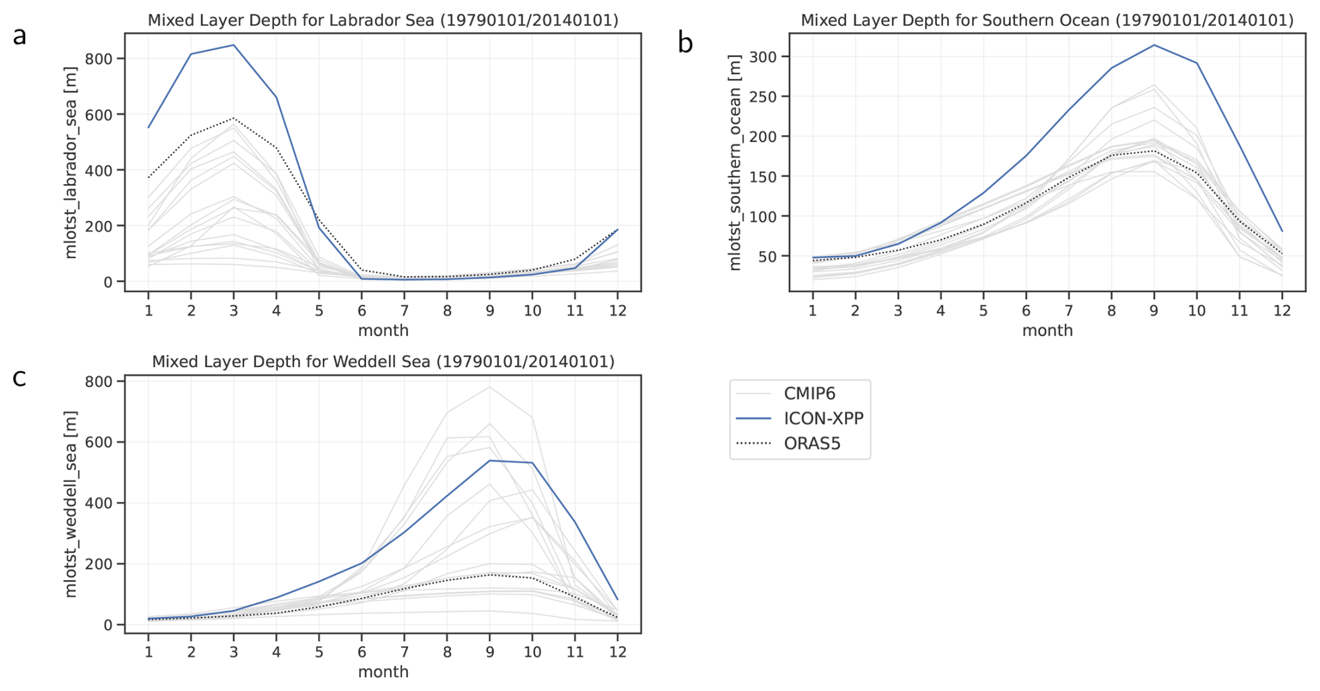
Figure 13 Seasonal cycle of the ocean mixed layer depth defined by sigma-T for ICON-XPP (blue line) compared with results from the CMIP6 ensemble (gray lines) and ORAS5 (black dashed line) for (a) Labrador Sea, (b) Southern Ocean, and (c) Weddell Sea for the period 1979 to 2014.

An important feature of the ocean circulation related to the MLD variability in the Labrador Sea and other areas with mode and deep water formation in the North Atlantic is the Atlantic Meridional Overturning Circulation (AMOC, Danabasoglu et al., 2014). The AMOC drives the inter-hemispheric northward transport of heat and salt at the surface (Zhang et al., 2019). In addition, several studies investigated a simulated AMOC collapse as a potential tipping point of the Earth system in climate projections (McKay et al., 2022). Thus, simulating the observed historical AMOC strength accurately is a key metric during ocean model development. Figure 14 shows the time series of the historical AMOC strength, defined as the maximum of the meridional mass stream function at 26.5° N in the Atlantic, for ICON-XPP, CMIP6 models and plotted against the observed AMOC strength from the RAPID array (Cunningham et al., 2007) from 2004 onward.

ICONEval and ESMValTool can be further used to monitor key oceanic climate metrics like the ocean heat content (OHC) during model development. The OHC is influenced by atmosphere-ocean interactions as well as by the MLD. As an example, Fig. 15 shows the OHC anomalies of the upper 300 m from ICON-XPP, some CMIP6 models and the EN4 and IAP reference datasets.

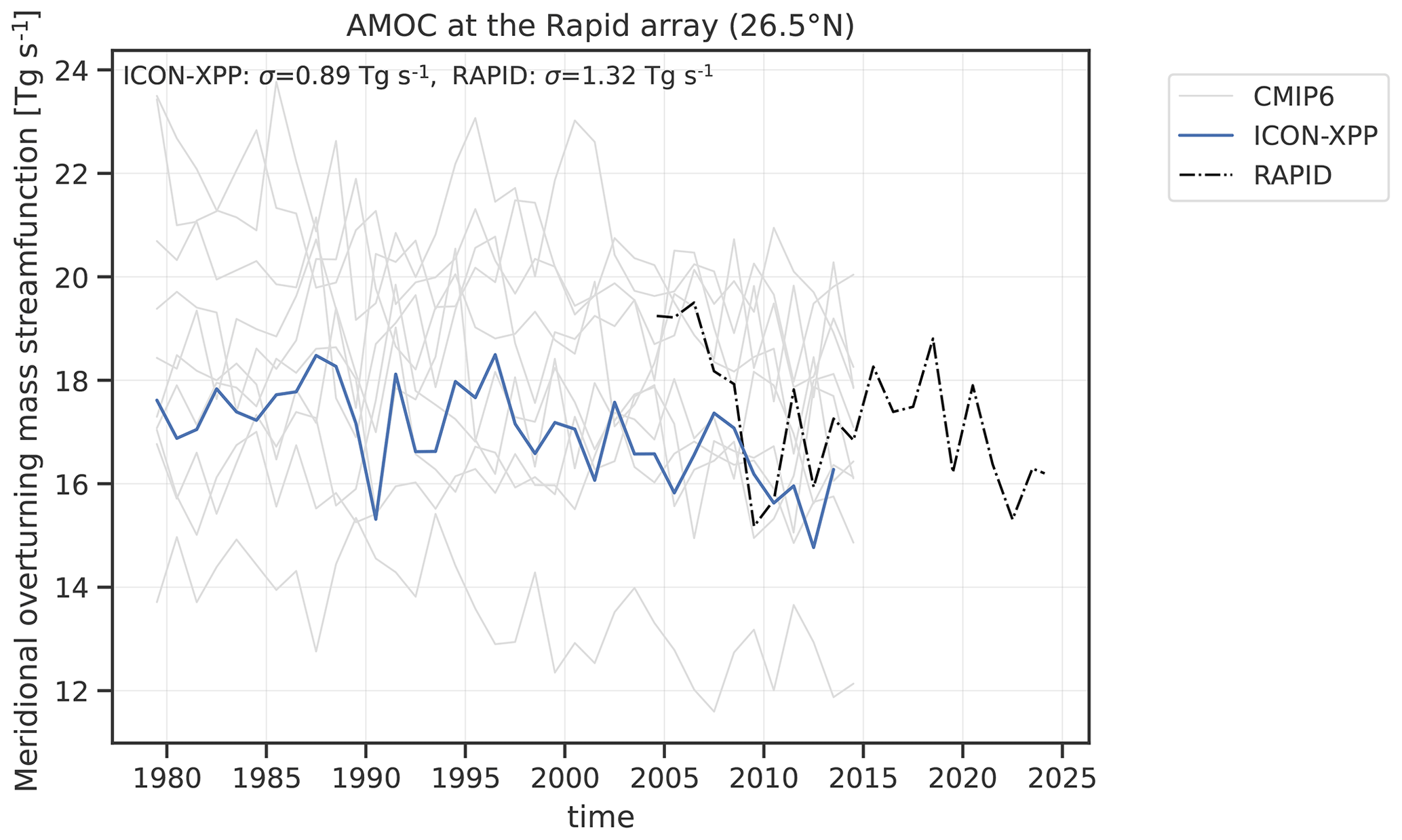
Figure 14 Time series of the AMOC strength calculated as the maximum of the meridional mass stream function at 26.5° N. The black dash-dotted line shows the RAPID observational data, the blue line the ICON-XPP results and the thin gray lines examples from the CMIP6 model ensemble. The temporal standard deviations (σ) for RAPID and ICON-XPP are given in the top of the panel. Historical ESM simulations are not expected to replicate the timing of the AMOC strength, but should have a comparable amplitude and frequency of the interannual variability.

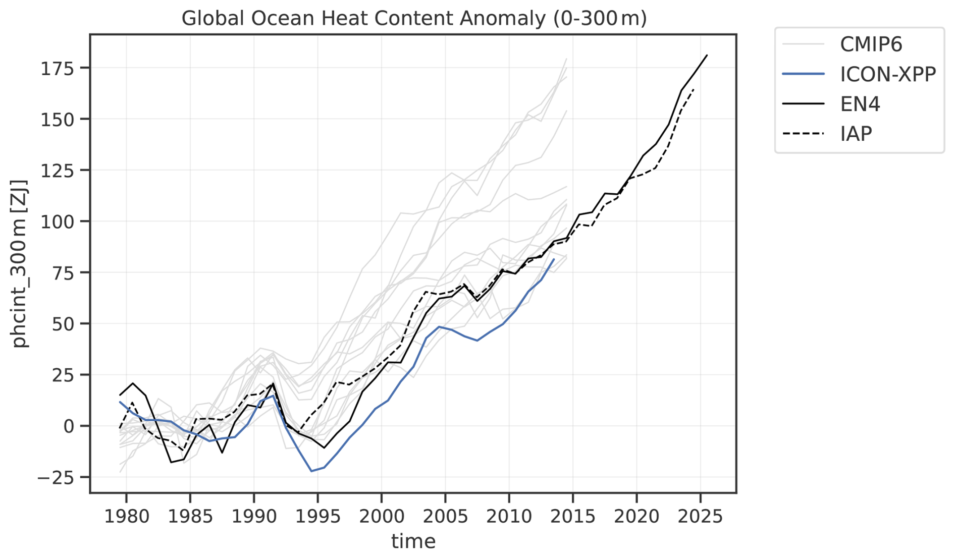
Figure 15 Time series of ocean heat content anomaly for the upper 300 m relative to the 1995–2014 average in zettajoules (ZJ). The black lines show the reference datasets, the blue line the ICON-XPP results and the thin gray lines results from the CMIP6 model ensemble.

5.3 Land

An important parameter for the land component is the surface temperature as this is one of the key parameters for coupling the land component with the atmosphere. Another important parameter is land evaporation, which plays a key role in the water cycle and land-atmosphere interactions.

The leaf area index (LAI, unitless) is a measure of the canopy structure and used by models to calculate the photosynthetic uptake of carbon of the total canopy (Park and Jeong, 2021). Maps of its geographical distribution can be used to identify areas with atypical growth. Figure 16 shows a 10-year average of LAI based on the example ICON-XPP simulation and LAI3g observations for the same period used as a reference. Highest LAI values can be found in tropical rain forest regions, for both datasets. The difference map in the bottom panel of Fig. 16 shows an overestimation in the simulated LAI by 0 to 2 for many regions in the Southern Hemisphere.

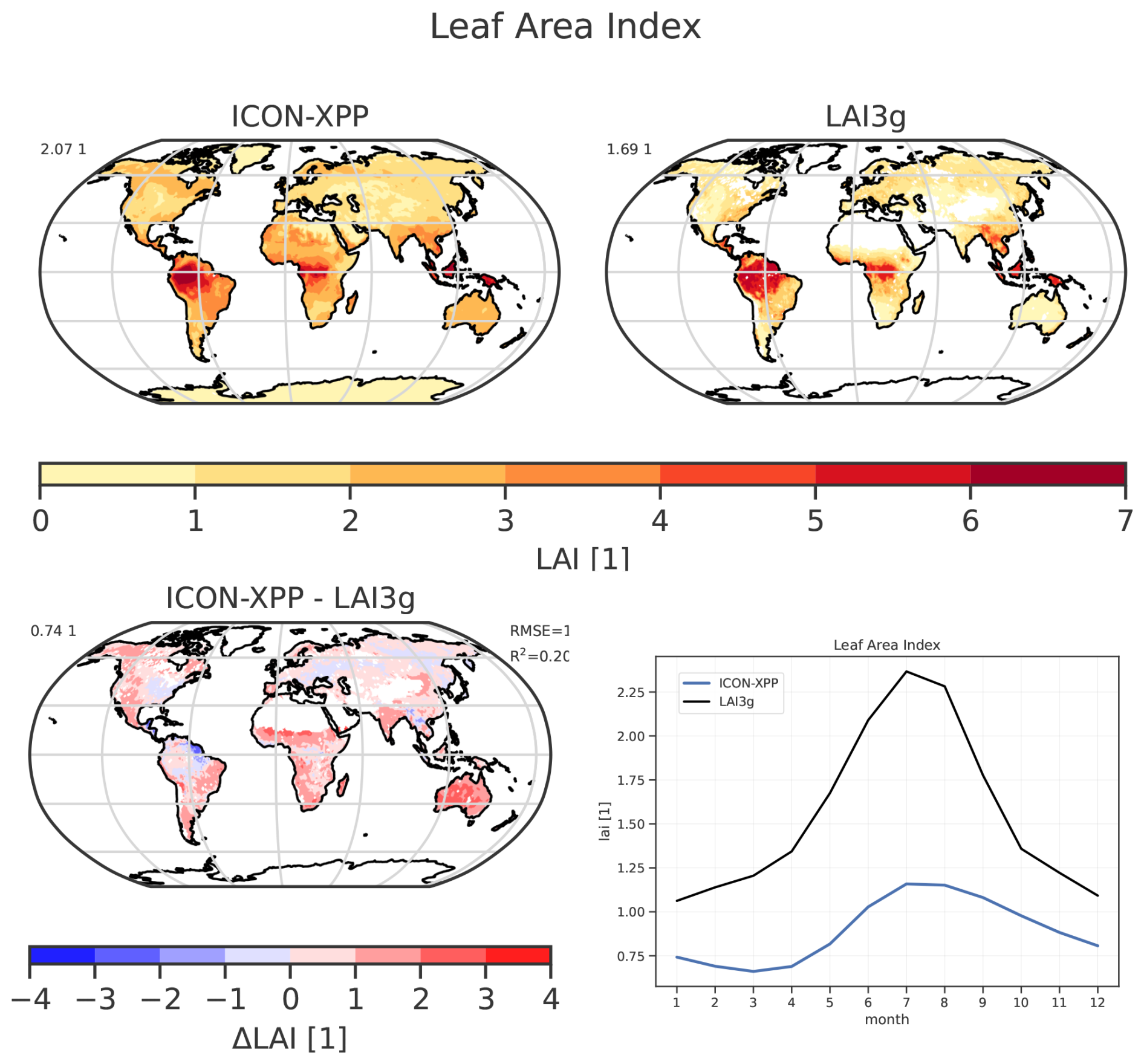
Figure 16 Average Leaf Area Index (LAI) from ICON-XPP averaged over the period 1995–2004 (top left), from the LAI3g observational dataset over the same period (top right) and their difference (bottom left). The average seasonal cycles averaged over the Northern Hemisphere are shown in the bottom right.

The seasonal cycle of LAI is expected to follow the growth season and to be particularly well defined in the Northern Hemisphere. The summer peak in July/August can be observed in the bottom right panel of Fig. 16, which shows a monthly NH climatology from ICON-XPP together with the LAI3g reference data. The generally higher LAI values in the NH climatology of the LAI3g dataset are caused by missing values in arid regions. ICON-XPP in contrast, provides full spatial coverage with generally small LAI in arid regions.

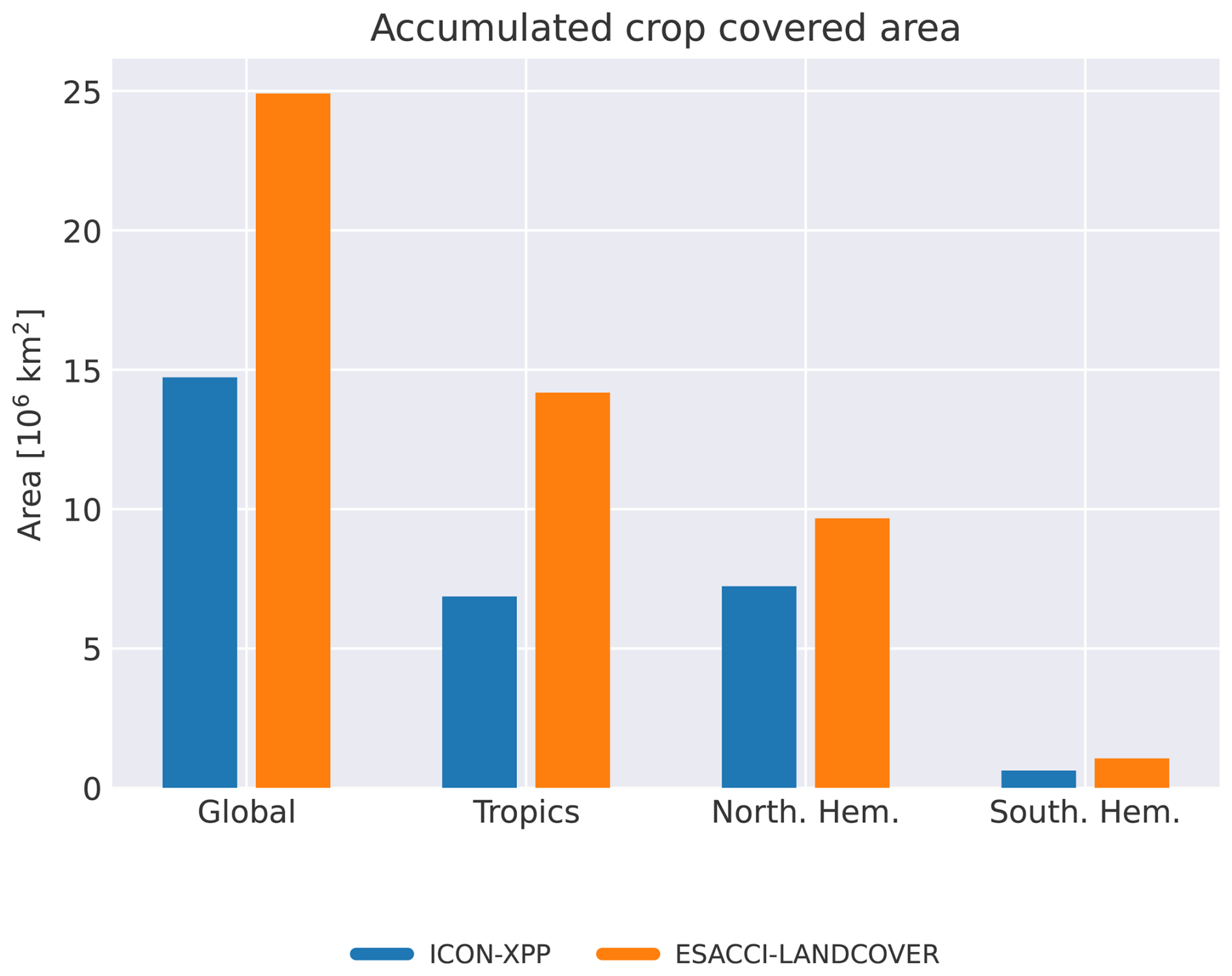
Figure 17 Total land area in million km² covered by crops from ICON-XPP (blue) in comparison with the ESACCI-LANDCOVER observational dataset (orange) for the regions (from left to right) global, Tropics, Northern Hemisphere, Southern Hemisphere.

To check the validity of the land model, the coverage of different land types can be compared to observations, as done in Fig. 17 for the example of crop area. This is particularly of interest for models with a dynamic vegetation. While this is important for checking how well a model does compared to observations, this is also highly relevant for regional modeling and impact assessment.

6 Summary and conclusions

As the output of Earth system models continues to grow in complexity and resolution, efficient and user-friendly tools can be a great support to assess, document and compare model performance across different model versions or configurations. This paper presents recent extensions of ESMValTool, and introduces ICONEval as an ESMValTool-based framework for rapid and physical consistency evaluation of ESMs. ICONEval is a wrapper designed to complement ESMValTool capabilities by providing a simplified access to a set of predefined evaluation tasks including sanity checks, physical consistency checks, and climate fidelity diagnostics of essential climate variables. The sanity checks are used for a first and very basic quality control to verify that the global mean values of key climate parameters of historical simulations are within reasonable ranges. These ranges are derived from upper and lower limits, i.e. maximum and minimum, of these parameters across multiple observational or reanalysis datasets and all monthly means available used for comparison. In addition, minimum and maximum values across all grid cells are analyzed to check that all values are physically reasonable, e.g. that mass mixing ratios are positive or maximum total cloud fraction does not exceed 100 %. Aspects checked include radiation and energy fluxes, atmospheric moisture and precipitation, integral cloud properties and cloud radiative effects, and near-surface temperature and wind stress. The physical consistency checks analyze compliance with fundamental physical laws and thermodynamic relationships. The checks implemented include e.g. conservation of the total mass of air, variability of global water vapor mass with temperature (Clausius–Clapeyron), the temperature dependence of the cloud ice fraction, and tropospheric lapse rate distributions for the Tropics and mid-latitudes. The consistency checks aim at identifying potential violations of physical constraints that could be introduced when implementing new or updating existing parameterizations. The third category of assessment recipes consists of selected basic model evaluation diagnostics that can be used to assess relevant key climate parameters across atmosphere, ocean and land in historical simulations, e.g. the time period for which observations are available. The diagnostics include evaluation of climatologies, geographical distributions, seasonal and diurnal cycles, and time series averaged over selected regions. Atmospheric parameters include e.g. temperature, precipitation, radiation, and humidity. Ocean variables include e.g. sea surface temperature, sea surface salinity, sea ice area, mixed layer depth, ocean heat content and selected ENSO indices. Land variables included are leaf area index, gross primary production, evaporation, surface temperature and land cover type. For all realms it is easily possible to expand the available recipes with additional diagnostics and observations. The new ICONEval capabilities are exemplarily demonstrated by applying the new diagnostics to a historical simulation from the ICON-XPP model. In addition to the expansions of recipes and the implementation of different checks, ICONEval automates the execution of predefined ESMValTool recipe templates and can run a large number of diagnostics in parallel. This allows for producing results quickly and thus allowing multiple assessments of a models' performance also during run-time of a simulation. The ICONEval framework further provides integrated visualization and reporting capabilities, including automatically generated HTML summary pages that can be published to a web server for interactive inspection via a standard web browser and easy sharing with collaborators outside the used HPC environment. This enables a continuous and user-friendly assessment of a model's performance during model development to quickly identify major problems such as unrealistic or physically inconsistent results. While initially focusing on evaluating ICON-XPP, extensions for other models are underway.

The extensions of ESMValTool together with the presented ICONEval framework provide a basis for an efficient, multi-step check for physical consistency and model performance across different ESM components tailored to the needs of modern climate model development. The implementation in ESMValTool allows for a relatively easy and straight-forward extension to additional components such as land-ice, biogeochemistry, etc. The described approach can support model developers during extension of the increasingly complex models and implementation of new parameterizations including machine learning–based schemes. This also supports emerging benchmarking efforts such as ClimateBench (Watson-Parris et al., 2022), where a consistent evaluation infrastructure is essential for placing data-driven and hybrid models on equal footing with physics-based ESMs. Sanity checks allow for quick identification of unreasonable results, physical consistency checks provide a quality control to prevent potential violations of fundamental physical laws such as conservation of mass or known thermodynamic relationships before assessing the models' performance and suitability for specific scientific applications in more detail. In combination with the benchmarking capabilities of ESMValTool for single models introduced in Lauer et al. (2025) and further extended and applied in the framwork of the CMIP7 REF (Hoffman et al., 2026), deviations of a model simulation from observational and reanalysis datasets used as reference can be put into context of other simulations with the same model but different model configurations or results from other ESMs such as the CMIP6 model ensemble.