DeepMelt-GL v1: a neural network emulator of sub-shelf melt rates for the unrepresented regions of ice-shelf cavities in ocean models

The spatial pattern of melting beneath Antarctic ice shelves influences ice flow and retreat, and the resulting freshwater input into the Southern Ocean influences global carbon storage and primary productivity. It is therefore crucial that interactions at the ice-ocean interface are adequately represented in global climate models. However, due to computational limitations, existing climate models are forced to choose between either high resolution or long period simulations, and struggle to resolve melt rates in ice shelf cavities. Here, we show that a simple multilayer perceptron can be used to emulate sub-shelf melt rates in entire small cavities and in the parts of large cavities closest to the grounding zone. We find that the melt rates produced by applying neural network emulators are a good match for melt rates from high resolution simulations, provided that similar conditions were included in the neural network training. We also find that neural networks are particularly sensitive to temperatures and ice-draft slopes outside those used in the training dataset. However, if we train multiple neural networks on the same input data, we demonstrate that the ensemble spread of the neural networks is a good indicator of the reliability of the emulator in any given conditions. The neural network emulator of sub-shelf melt which is presented here, DeepMelt-GL, can be used to improve the representation of ice shelf cavities in both ocean and climate models.

1 Introduction

The mass loss of the Antarctic ice sheet has led on average to a freshwater input of 2680 Gt yr⁻¹ to the Southern Ocean over the period 1997 to 2021 (Davison et al., 2023). 40 % of this freshwater (1080 Gt yr⁻¹) enters the ocean at a few hundred meters depth, in the form of meltwater originating at the base of the ice shelves, the floating margins of the ice sheet. This meltwater has local and global implications for the ocean, driving overturning circulation, affecting low-latitude primary productivity and influencing the oceanic carbon sink (Gruber et al., 2019; DeVries, 2014), as well as being a driver of mass loss from the grounded Antarctic Ice Sheet (Rignot, 2002; Pritchard et al., 2012). As the volume of meltwater from the base of ice shelves is predicted to increase in the future (Timmermann and Hellmer, 2013; Jourdain et al., 2022; Naughten et al., 2023; Mathiot and Jourdain, 2023; Burgard et al., 2025), it is crucial that future climate projections include coupled ocean-ice-sheet models which capture both the response of ocean properties to changing volumes of sub-shelf melt, and the response of sub-shelf melt to changing ocean properties and evolving cavity geometry.

Current modelling approaches which account in some way for sub-shelf ice-ocean interactions include prescribed freshwater fluxes from external climatologies in global ocean models (Merino et al., 2018; Hutchinson et al., 2023), some regional and global coupled ocean-ice-sheet models (Timmermann and Goeller, 2017; Bett et al., 2024; Smith et al., 2021), and sub-shelf melt rates calculated from far-field ocean conditions in continental ice-sheet models (DeConto and Pollard, 2016; Jourdain et al., 2020; Seroussi et al., 2024). Global ocean models used in climate models for multi-decadal and centennial simulations usually work on a grid resolution of approximately 1° (∼56 km at 60° S, ∼30 km at 75° S). Many models do not consider sub-ice-shelf cavities, and as a result the freshwater flux into the ocean from sub-ice-shelf melt is prescribed by redistributing a fraction or all of the surface mass balance (precipitation minus sublimation and runoff) of the Antarctic continent into the ocean surrounding the continent (Schmidt et al., 2025). This is mostly done to conserve the ocean volume in the climate simulations, but neglects changes in freshwater fluxes due to ice sheet dynamics. It is rare that ocean circulation within ice-shelf cavities is resolved within global ocean models, and it was not in any of the models in the Coupled Model Intercomparison Project Phase 6 (CMIP6) (Eyring et al., 2016; Heuzé, 2021). This is one of the reasons why the modelled ocean behaviour around the Antarctic continent often does not match observations of water properties (Heuzé et al., 2013; Chen et al., 2023). Although regional ocean models that resolve the ocean circulation below ice shelves are becoming more common (Yung et al., 2026), they are not always designed for multi-centennial or ensemble simulations, due to computational limitations (Holt et al., 2017).

First steps have been made towards the representation of the ocean circulation below ice shelves in ∼1° ocean models (e.g. Beckmann et al., 1999; Smith et al., 2021; Hutchinson et al., 2023). However, at 1° resolution, while cavity circulation in the largest ice-shelves (such as Ross, Filchner-Ronne, Larsen C) is represented, smaller ice shelves with high observed melt rates (such as Thwaites, Pine Island and Totten, Davison et al., 2023) and all grounding lines remain unresolved or poorly resolved (Smith et al., 2021). This limits our ability to assess the consequences of both the effect of sub-shelf meltwater on the ocean and the localised effects of sub-shelf melt on the ice sheet dynamics and mass loss.

Continental ice-sheet models need sub-shelf melt forcing for all ice shelves. Currently, a range of parameterisations can be applied to infer sub-shelf melt patterns from non-cavity resolving global ocean models (Burgard et al., 2022; Lambert et al., 2023). However, these parameterisations often fail to reproduce the spatial melt rate patterns (Burgard et al., 2022), especially in warmer ocean conditions representative of future climates (Burgard et al., 2023; Lambert and Burgard, 2025; Beckmann et al., 2025). Although these parameterisations represent an improvement on the prescribed melt used in ocean models, alternative approaches which fully capture the feedbacks between ocean properties, ice shelf-geometry and sub-shelf melt are needed to facilitate multi-centennial, ensemble, coupled simulations. An option is to use an intermediate system that couples an ice sheet and an ocean model using these parameterisations (Kreuzer et al., 2021; Sadai et al., 2025). Another alternative is to leverage machine learning techniques to emulate melt rates from high resolution models.

Supervised machine learning offers the opportunity to use high resolution simulated datasets to improve the parametrisation of the relationship between sub-shelf melting and water properties as resolved in a global ocean model. Using different architectures, Rosier et al. (2023) and Burgard et al. (2023) both showed that simple neural networks can reproduce ice-shelf melting patterns produced in model simulations, and that, in warmer conditions, neural networks have a lower error when compared to reference melt rates than the majority of traditional parameterisations. In both studies, neural networks were used to parametrise the whole of the ice-shelf cavity for use with stand-alone ice-sheet models. Since some ocean models include ice-shelf cavities, here we explore the suitability of using neural networks to parametrise the parts of cavities which are not resolved in these ocean models. For small cavities, this is the entire cavity, whereas for large cavities this means just the part closest to the grounding line. This approach allows us to maintain the full physics of water flow in ice-shelf cavities where resolved, and to produce sub-shelf melt patterns for the entire cavity.

In this study, we investigate the advantages and limitations of a neural-network emulator of the sub-shelf regions not resolved in the 1° version of the NEMO ocean-sea-ice model (Nucleus for European Modelling of the Ocean, Madec and the NEMO System Team, 2024), which we train using NEMO simulations with a resolution of 0.25° (4–14 km around Antarctica). Using selected input conditions, we explore the emulator performance in similar conditions to the training data, in conditions outside the training data, and with limited quantities of training data. We produce an emulator which can be used in the NEMO global ocean model, and make recommendations about the conditions in which the neural network emulator can be reliably used.

2 Methods

This study aims to explore whether a neural network can be trained to emulate sub-shelf melting in parts of the ice-shelf cavity not resolved by a 1° ocean model, by identifying relationships between the water properties from the ocean model, the geometry of those cavity regions, and the sub-shelf melt rates simulated in relatively higher resolution (0.25°) models. Alongside this manuscript, we provide a neural network trained using all available NEMO 0.25° simulations for application in stand-alone ocean models or coupled systems. However, in order to better understand the conditions in which this trained neural network can be expected to perform well, we additionally trained neural networks on specific individual simulations. Here, we discuss the ocean model simulations that we aim to emulate, the architecture of the neural network used for emulation, and the experimental procedure through which neural network performance is assessed.

2.1 Data: simulated ice-ocean conditions

This work aims to produce a neural-network emulator of the sub-ice-shelf regions not resolved in the 1° version of the NEMO ocean-sea-ice model (Nucleus for European Modelling of the Ocean, Madec and the NEMO System Team, 2024). In order to do this, we employ a selection of NEMO simulations of ocean conditions run on the eORCA025 or eANT025 grids, which are global (Mathiot and Jourdain, 2023) and regional circum-Antarctic (Olivé Abelló et al., 2025; Pirlet et al., 2025) grids with a resolution of 0.25° (4–14 km around Antarctica). We use simulated melt rates as our “reference” melt rates because there are currently insufficient simultaneous observations of melt-rate and water properties, and because this allows us to include future climatic conditions which have not yet been observed. We stress that model parameters in the NEMO ocean model are tuned using estimated sub-shelf melt rates and water properties from the last 40 years (Mathiot and Jourdain, 2023). We focus on grid cells which are resolved as ocean points beneath the ice shelf in the 0.25° simulations, but which would be defined as land in the corresponding 1° model (Fig. 1). In all simulations, sub-shelf melt is calculated using the widely-used three-equation thermodynamic system that accounts for the heat and salt balances at the ice-ocean interface, and the pressure and temperature dependence of freezing temperature (Holland and Jenkins, 1999; Asay-Davis et al., 2016; Mathiot et al., 2017).

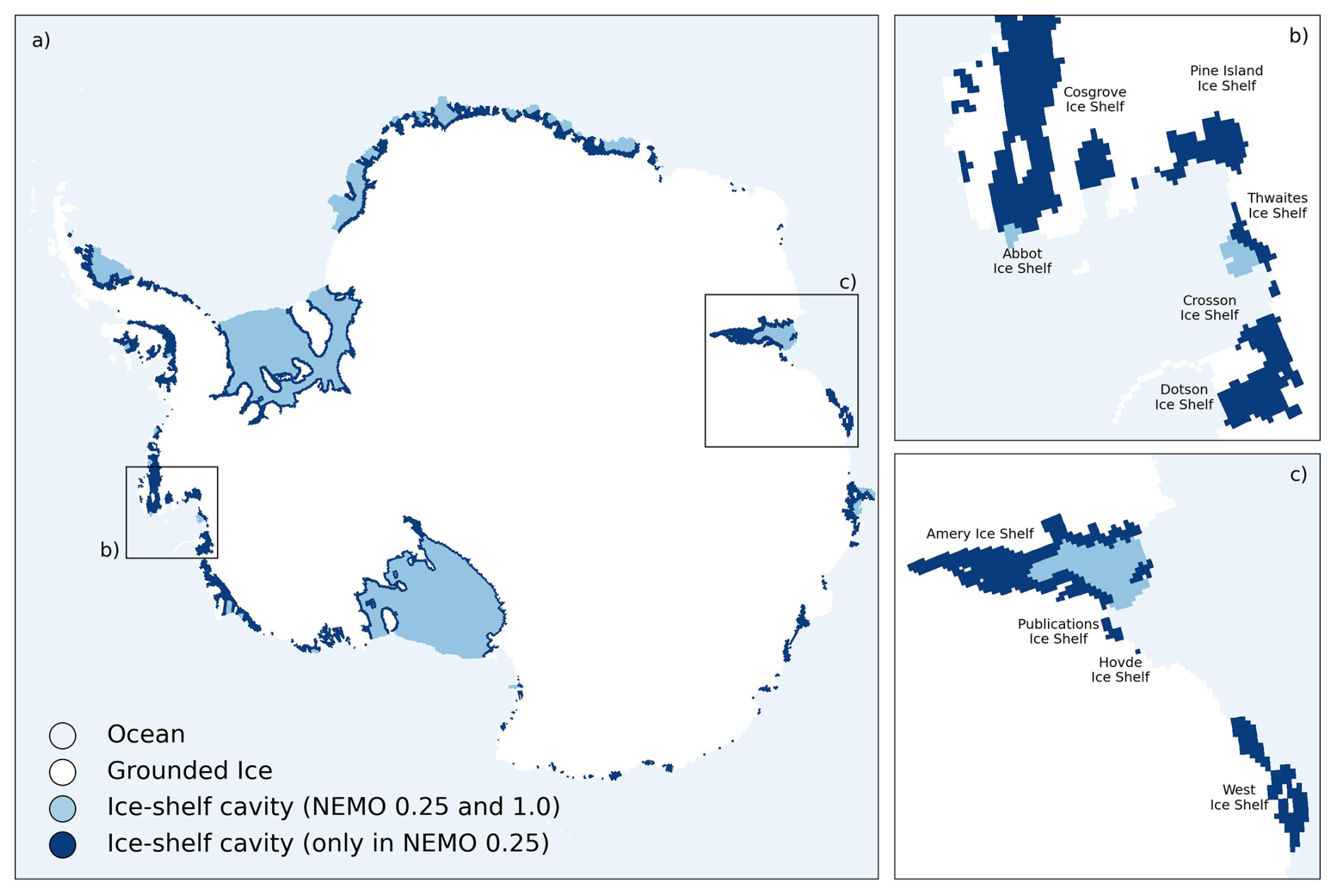
Figure 1 The spatial distribution of ice-shelf cavities which are resolved in the NEMO model at 0.25 and 1°. Panel (a) !shows the distribution of cavities resolved at 0.25° (dark and light blue) and the ones that would be resolved at 1.0° (light blue only) for the whole Antarctic continent, illustrating that although the largest ice shelves are resolved in the 1.0° model, many important and fast-changing regions require a higher resolution for sub-ice shelf dynamics to be included in ocean models. Panels (b) and (c) show zoomed-in insets for the Amundsen Sea sector and Amery Ice Shelf as examples. We use the regions which are only resolved in the 0.25° simulations (dark blue) for training the neural network, with ocean properties there propagated from the area that would be resolved at 1° (light blue area).

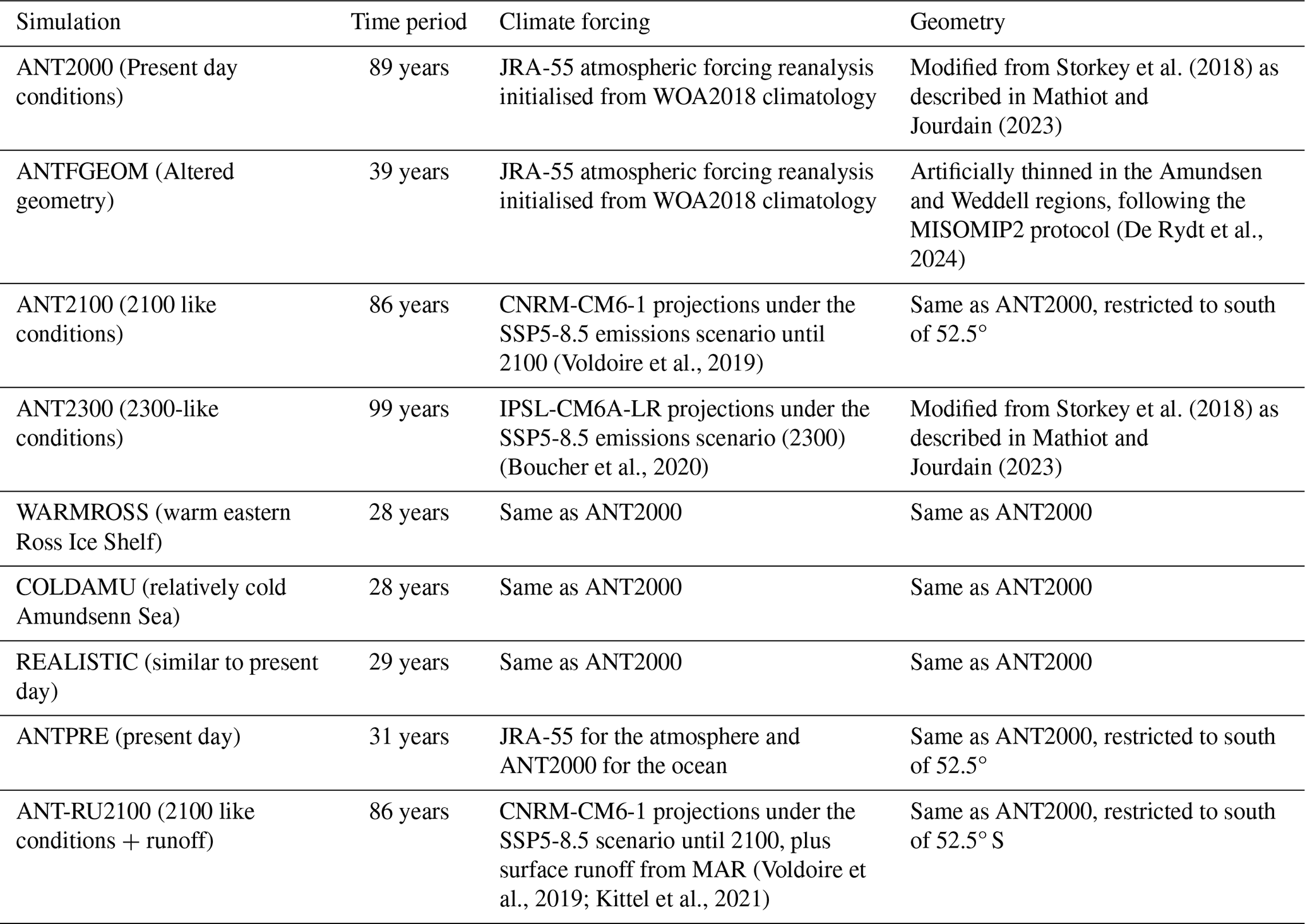
To assess the performance of neural networks as emulators of sub-shelf melt in these partial cavity regions, we use monthly data from four different NEMO simulations (ANT2000, ANTFGEOM, ANT2100, ANT2300, differences summarised in Table 1). Using monthly data allows us to increase the volume of training data and cover a larger range of input conditions. We use two simulations with present-day forcing, both driven by the JRA55-do atmospheric reanalysis (Tsujino et al., 2018) and initialised in 1979 from the climatological WOA2018 conditions (Mathiot and Jourdain, 2023). In the first present-day simulation, which we call ANT2000, bathymetry and ice shelf draft are a modified version of those used by Storkey et al. (2018), updated to be closer to Bedmachine Antarctica v2 on the Antarctic continental shelves (Morlighem et al., 2020) and with some other small modifications as described in Mathiot and Jourdain (2023). In the second, which we call ANTFGEOM, ice shelf draft is artificially thinned in the Amundsen and Weddell Sea regions and the grounding line retreated, following the MISOMIP2 protocol (Fig. A1, De Rydt et al., 2024), to be representative of a possible future geometric configuration, but it is still driven by present-day atmospheric conditions. There are also some small differences in the geometry in other ice shelf basins (Fig. 6).

We also use two simulations which simulate plausible future ocean conditions. Both use the same ice-shelf draft and bathymetry as ANT2000. The first of these simulations, which we call ANT2100, uses a climate forcing driven by continuous atmospheric and oceanic anomalies from the CNRM-CM6-1 projections under the SSP5-8.5 scenario (Voldoire et al., 2019) until 2100, added to the climatology. ANT2100 is restricted to a regional domain south of 52.5° S. The second simulation, which we call ANT2300, is global and applies a temperature anomaly extracted from the IPSL-CM6A-LR projections under the SSP5-8.5 emissions scenario (Boucher et al., 2020; Lurton et al., 2020), in order to explore potential extreme conditions at the end of the 23rd century. Further details about the exact parameters used in these simulations can be found in Mathiot and Jourdain (2023).

Additionally, at the end of this study we present a neural network emulator that has been trained on all available 0.25° simulations which we have access to. In addition to the monthly data from the four simulations described above, we also use annual data from five additional simulations. Three of these simulations (WARMROSS, COLDAMU, REALISTIC) were part of the ensemble used for training in Burgard et al. (2023), and have the same forcing and bathymetry as ANT2000 but vary in the parameters used for oceanic behaviour. Further information about these simulations can be found in Burgard et al. (2023). The remaining simulations (ANTPRE, ANT-RU2100) use the same regional ocean model configuration as ANT2100. ANTPRE is forced by JRA-55 for the atmosphere and by the present-day ocean simulation of ANT2000 for the ocean. ANT-RU2100 uses the same climate forcing as ANT2100, but with the addition of surface runoff from MAR as an additional freshwater source (Kittel et al., 2021).

Table 1 Description of the climate forcing and geometry employed in for the simulations used in this study. All simulations have a resolution of 0.25°. WARMROSS, COLDAMU and REALISTIC vary in their internal model parameters (Burgard et al., 2022).

2.1.1 Spatial focus

This study aims to develop a neural-network emulator for use in coupled ice-sheet-ocean modelling, which allows as much of the ocean and ice-shelf cavity to be resolved in the ocean model as possible. Therefore, we train the neural network only in regions where the sub-shelf cavity is resolved in the 0.25° model, but which are considered to be grounded ice in a hypothetical equivalent 1° model (Fig. 1, dark blue). Regions which would be resolved as sub-shelf cavity in the 1° model are not included. For small ice-shelves, this means emulating the entire ice shelf. However, for the largest ice shelves, we only need to emulate a relatively thin strip around the innermost edge of the ice shelf. In order to have a flexible framework which can adapt to evolving shelf geometries and changing grounding line positions, we divide the coastline of Antarctica into 155 partial ice-shelf basins, based on the locations of the individual outlet glaciers and ice streams (see Appendix A2, Mouginot et al., 2017). Large pinning points (ice rumples and rises) are also separated and form their own basins. These basins are extrapolated into the open ocean using a nearest neighbour approach, and occasionally adjusted manually to ensure that basins which contain an ice-shelf front always have a few points in the open ocean. The resulting partial ice-shelf basins all have similar dimensions, with the exception of basins which include islands and are not part of the main coastline. The margins of the largest ice-shelves fall into several of these partial ice-shelf basins.

2.2 Neural network

Supervised machine learning offers the opportunity to use high-resolution simulated datasets to improve the parametrisation of the relationship between water properties and sub-ice-shelf melting. Simple neural networks can leverage computational data structures to identify relationships between ocean conditions and sub-ice-shelf melt rates that would otherwise be difficult to identify in this multi-dimensional data set (Rosier et al., 2023; Burgard et al., 2023). We use a pointwise neural-network architecture based on the multilayer perceptron used by Burgard et al. (2023) to predict sub-ice-shelf melt rates using information on the sub-shelf geometry and ocean conditions.

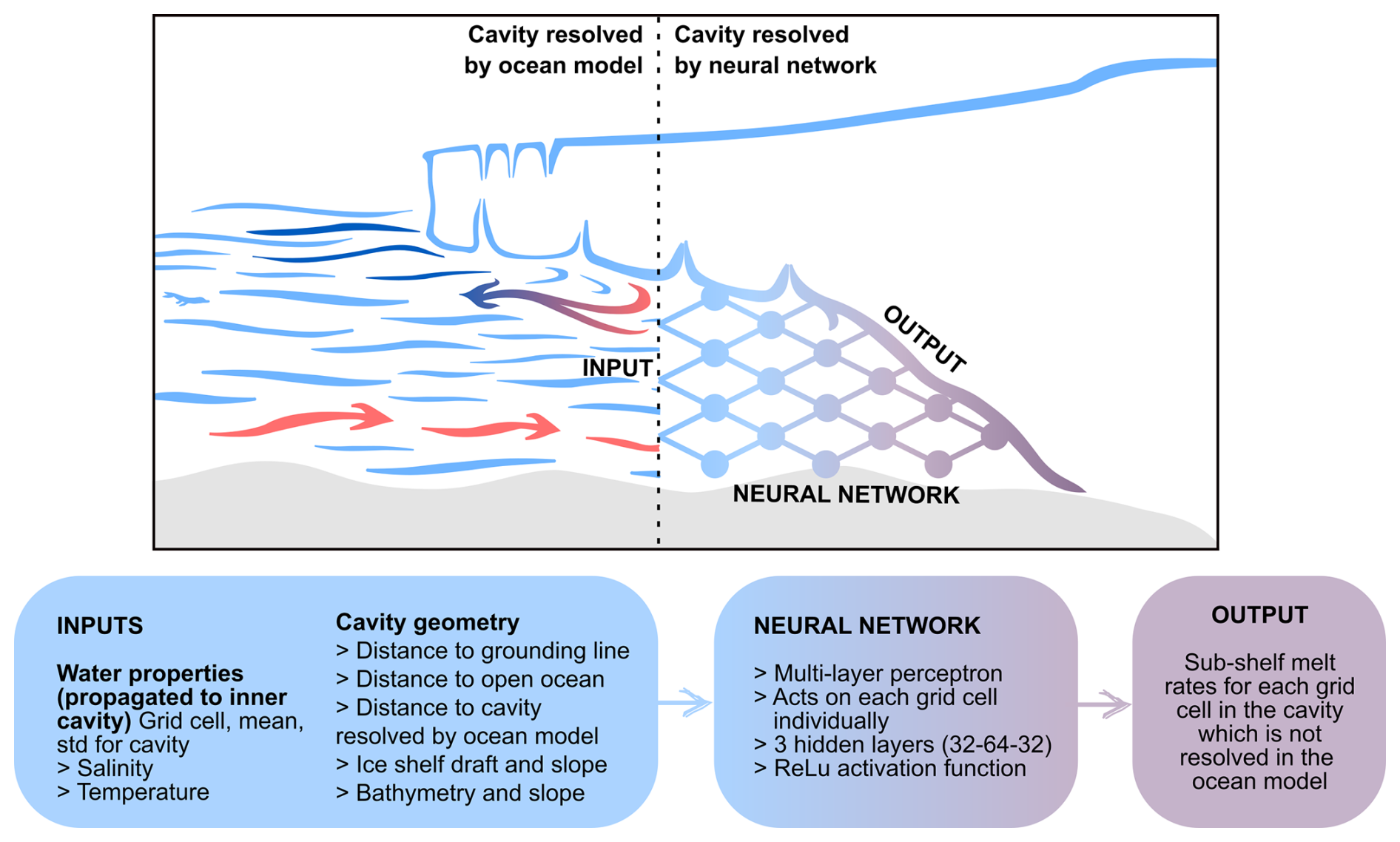
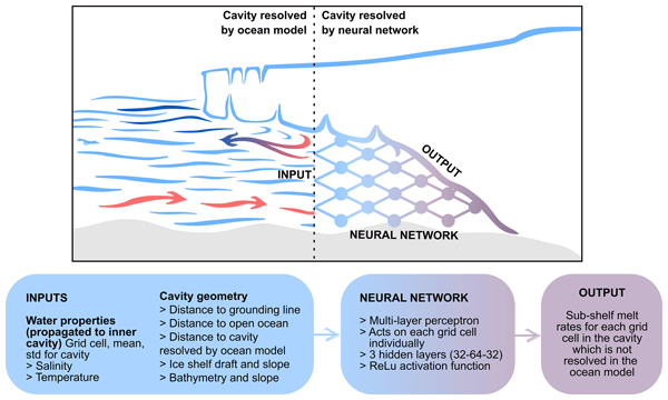
Figure 2 The key inputs and outputs involved in the neural network training and application. Water properties and cavity geometry are separate classes of input properties because water properties come from the edge of the cavity as resolved in the 1° ocean model, and cavity geometry comes from the region which is not resolved in the 1° ocean model. In training, cavity geometry is the one prescribed in the NEMO model, but in a coupled ocean-ice-sheet model the geometry would come from the ice-sheet model.

2.2.1 Architecture and hyper-parameters

Following Burgard et al. (2023), we use a simple multilayer perceptron implemented using the keras package in python (Chollet, 2015), which has multiple input variables and a single output variable: sub-shelf melt rate. As we consider a slightly different spatial domain, comprising a mixture of entire small ice shelves and the peripheral strip of larger ice shelves, we have a slightly different set of input parameters than Burgard et al. (2023) (see Sect. 2.2.2). Inputs are processed through three sets of computational layers of artificial neurons (hidden layers), which apply weightings and non-linear activation functions, allowing the neural network to represent complex non-linear relationships. We use three hidden layers of 32, 64 and 32 neurons respectively, as this small neural network size was previously found to give good results in cross validation tests over both time and cavity geometry without over-fitting input data (Burgard et al., 2023). During the neural network training process, initially randomised weights are optimised with a gradient descent algorithm (Adam, Kingma and Ba, 2017) which is tuned to reduce the mean-squared error (mse) of the reference melt rates from the simulation data relative to the predicted melt rates from the neural network. We use an initial learning rate of 0.001, and a ReLU activation function (Fukushima, 1975; Ramachandran et al., 2017).

To assess the performance of the neural network training, and to avoid over-fitting the data, we use a validation data set containing a randomly chosen 10 % of the shuffled training data, which is separated before training begins. We explore the impact of these stochastic processes on the performance of the neural network by applying the same training process initialised with 10 different random seeds, giving us an ensemble of neural networks. Further information on the choice of neural network architecture and hyper-parameters can be found in Burgard et al. (2023).

2.2.2 Input variables

The neural network is trained and applied to an array of variables calculated at each grid point individually. Similarly to Burgard et al. (2023) we employ two different types of variables: information about the geometry of the ice-shelf cavity in the grid cell, and information about the water properties (temperature and salinity) at the front of the partial ice-shelf cavity. For both training and testing, we compare the output of the neural network to reference sub-shelf melt rates from 0.25° ocean simulations.

Geometrically, we provide the following variables: the distance to the closest point on the grounding line, the closest point in the open ocean, the closest point in the open part of the same cavity (if there is one resolved at 1°), the depth of the ice-shelf draft, and the bathymetry. Unlike Burgard et al. (2023), who calculated the meridional and zonal slopes, we calculate the slope of the ice-shelf draft and bathymetry both parallel and perpendicular to the front of the closed cavity (resolved at 0.25° but not 1°), in order to better account for ice shelves (or ice-shelf segments) that are not oriented facing north. The orientation of the cavity front is calculated using the mean locations of cavity grid points and the mean locations of ocean points along the front of the cavity.

Hydrographically, some pre-processing of the data is required. In order to have a point-wise neural network architecture, we need information about the temperature and salinity at each point. However, as the aim of the neural network is to emulate these cavities to be eventually used in a NEMO 1° model, the neural network must be trained with water property information which is available at that resolution. As a result, for each of the 155 partial ice-shelf basins, we calculate a mean temperature and salinity profile for the closest ocean points that would be resolved in the corresponding 1° model, which can be either open ocean or open cavities. We identify these points using a kdtree algorithm. We then infer water properties for each grid point in the emulated region by taking these properties from the mean profile at the same depth as the grid point. Additionally, to provide some information about the spatial variability of water properties, we also include the mean and standard deviation of the temperature and salinity across the partial ice-shelf basin. Unlike Burgard et al. (2023), who used potential temperature and practical salinity, we use conservative temperature and absolute salinity, which improves conservation in the propagation and reduces the data pre-processing needed as these are used in the NEMO ocean model.

2.3 Experiments and metrics for evaluation

Using monthly data from the four ocean simulations (ANT2000, ANTFGEOM, ANT2100, ANT2300) and the neural network architecture outlined previously, we carry out several experiments to explore the performance of the neural network emulator. For initial model verification, data from each of the four simulations was used to train the neural network, and model performance was verified for those simulations. In all other experiments, data from one or more simulations is used to train the neural network, and then data from a different simulation is used to assess the performance of the emulator in a range of conditions.

For each experiment, we report a range of metrics for emulator performance. Firstly, we report the root-mean-squared error (RMSE) of the predicted melt rate compared to the reference simulated melt rate, since MSE is the variable optimised during the neural network training, and this is a standard metric in machine learning. However, as we have data which vary both spatially and temporally, we also focus on metrics which allow us to explore those dimensions. Specifically, we look at the integrated melt on annual and monthly timescales, and grouped by regional ice-drainage basins as defined by the Ice sheet Mass Balance Inter-comparison Exercise (IMBIE, Rignot et al., 2019). In addition to the RMSE, we also report the correlation coefficient (R²) between the predicted and the reference melt for integrated melt rates.

We carry out three main sets of experiments, in each case training the neural network with one simulation, and testing the quality of the results by applying the trained neural network to an independent simulation. Firstly, we explore the performance of the neural network emulator in different climatic conditions to those used for the training, using the ANT2000, ANT2100 and ANT2300 simulations, which have almost identical geometries but differing water column temperature and salinity. Secondly, we explore the performance of the neural network emulator in different geometric conditions, using the ANT2000 and ANTFGEOM simulations, which have the same climatic forcing, but different geometries. Since all 155 partial ice-shelf basins have different geometries, we would expect that a neural network trained on the ANT2000 data set should give good results on a simulation where the geometries of the basins have changed. Finally, we explore the impact of the quantity of training data on the performance of the neural network, by training neural networks with data from part of the ANT2300 simulation, and testing on the ANT2100 simulation.

All tests which we describe here use monthly data, in order to increase the size of the training data set, and to ensure that it encompasses as wide a range of conditions as possible. Additional training and testing on both annual and monthly data shows that the neural network performance is significantly improved by using monthly data, due to the improved representation of extreme melt values in the training dataset. More information about these additional tests can be found in Appendix A3.

3 Results

3.1 Model verification

We verify that the neural network architecture can return realistic melt rate values by applying a trained neural network model to the same dataset used for training. For all four simulations used here, there is a strong correlation between the reference melt and the predicted melt rates for both the non-integrated pointwise melt (R² between 0.86 and 0.94) and the spatially integrated monthly melt rates (R² between 0.92 and 0.96). Where the correlation is better for integrated melt rates this is likely due to the cancellation of errors. The full set of metrics including RMSE for the model verification can be found in Fig. A5.

3.2 Does the NN parameterisation work in different climatic conditions?

To explore the adaptability of the neural network to different climate scenarios, we trained on the ANT2000, ANT2100 and ANT2300 simulations, which have almost identical geometries, but differing water column temperature and salinity. The maximum grid-cell melt rates are 117 m yr⁻¹ for the ANT2000 simulation, 181 m yr⁻¹ for the ANT2100 simulation, and 495 m yr⁻¹ for the ANT2300 simulation (metres of ice equivalent per year).

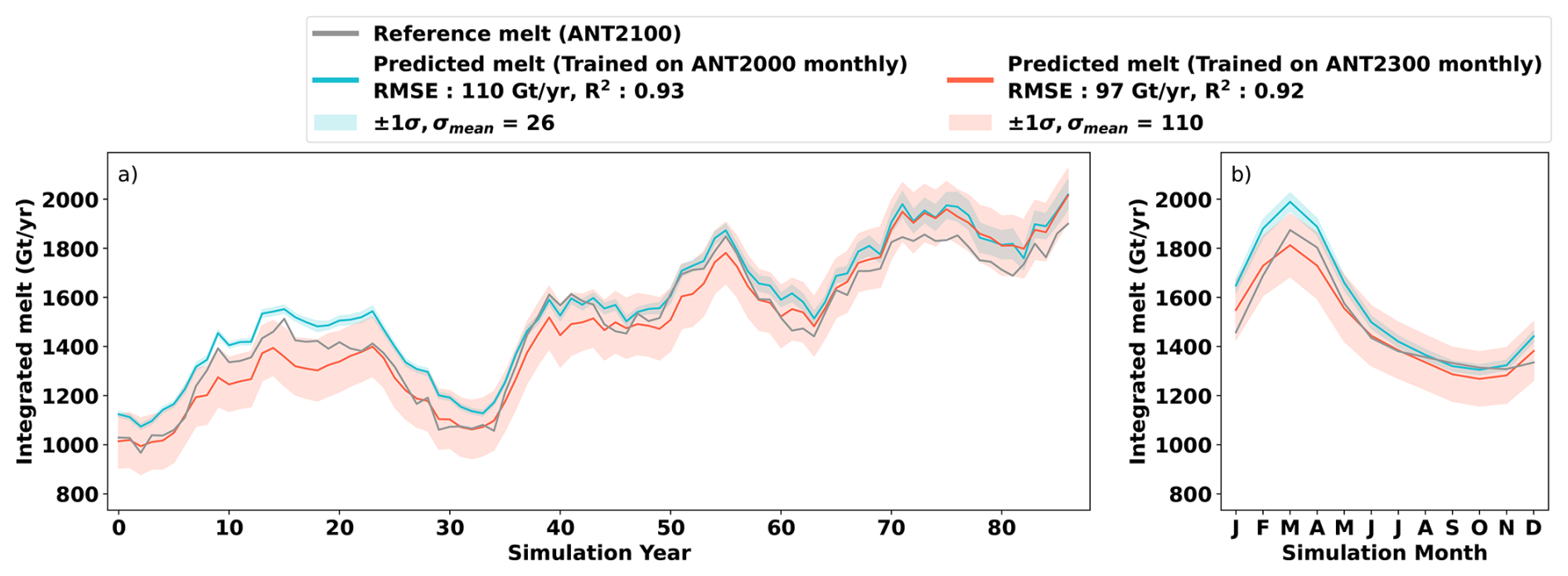
Figure 3 Neural network performance in temperature conditions outside the training dataset. The reference melt rates from the ANT2100 simulation (grey), compared to the predicted melt rates from neural networks trained on monthly data from the ANT2000 (blue) and ANT2300 (red) simulations, grouped into annual time series (a) and mean seasonal cycle (b) trends. Melt rates are integrated melt rates for the whole of Antarctica in Gt yr⁻¹, to allow the same scale for annual and monthly trend. The ensemble spread of the 10 neural networks is shown through the error bounds of one standard deviation.

Firstly, we consider a neural network trained only with data from the ANT2000 simulation, representing present day conditions. When this neural network is applied to the ANT2100 simulation, which represents warm 2100-like conditions, we find a good match between the integrated melt predicted by the neural network and the reference melt (Fig. 3, RMSE = 110 Gt yr⁻¹, and R²=0.93). The ensemble spread (standard deviation of the ten ensemble members) is 26 Gt yr⁻¹, highlighting a good agreement between ensemble members and a well constrained parameter space. This result shows that the neural network emulator can be applied to climate conditions outside the conditions in the training dataset and still produce realistic melt values.

When the ANT2000-trained neural network is applied to the ANT2300 simulation, which represents a hot 2300-like climate, we see that the neural network consistently under-predicts the melt rate (Fig. 4, RMSE = 2220 Gt yr⁻¹, R²=0.70). We note that in this case the ensemble spread is 750 Gt yr⁻¹, indicating that the neural network emulator is poorly constrained in this parameter space. These results demonstrate a limitation of these neural networks; if applied to conditions which are too different to the training dataset, the predicted melt rates will not match the expected melt rates.

Next, we consider a neural network trained only with data from the ANT2100 simulation, representing warm 2100-like conditions. When this neural network is applied to the ANT2300 simulation, which represents a hot-2300 like climate, we see an improvement in the results relative to the ANT2000-trained neural network (Fig. 4a, RMSE = 810 Gt yr⁻¹, R²=0.93). Although the ANT2100 neural network still under-predicts the melt rate, especially at the end of the ANT2300 simulation, the predicted and reference melt rates diverge later in the simulation and at a higher integrated melt value. This suggests that there is a threshold above which the neural network performance begins to degrade, which is controlled by the training data. Looking at RMSE as a function of conservative temperature and absolute salinity (Fig. 5), we see that reducing salinity does not affect RMSE as much as increasing temperature, and so suggest that this threshold is likely to be a temperature threshold.

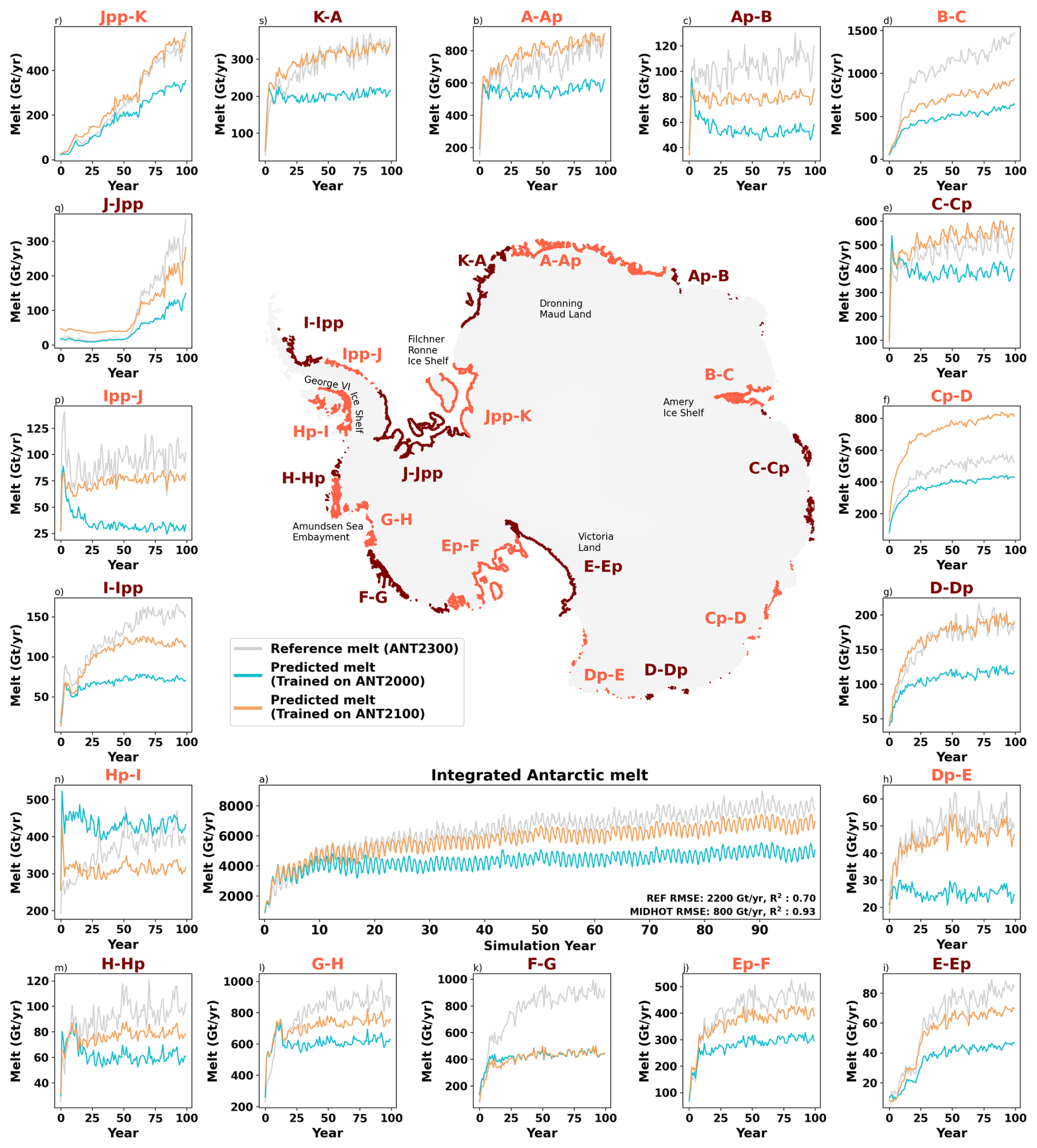
Figure 4 Neural network performance in temperature conditions outside the training dataset and in each of the IMBIE glacial drainage basins. A comparison of the reference melt rate from the ANT2300 simulation (grey) with the predicted melt rate from neural networks trained on monthly data from ANT2000 (blue) and ANT2100 (peach) to each glacial drainage basin in the ANT2300 simulation. (a) Integrated melt rates for the whole of Antarctica. (b–s) Integrated melt rates for each of the IMBIE glacial drainage basins. The location of each basin is shown in the central inset map. Regions which are discussed in the manuscript are labelled.

To assess spatial patterns in the the sub-shelf melt, we also consider the results of applying both the ANT2000 and ANT2100 neural networks to the ANT2300 simulation on a basin scale (Fig. 3). We use the glacial drainage basins defined by the Ice-sheet Mass Balance Inter-comparison Exercise (IMBIE). In many basins we see that both neural networks underpredict the melt, but the RMSE is lower for the ANT2100 neural network as it under-predicts by a smaller volume (Ap-B, B-C, E-Ep, Ep-F, G-H, H-Hp, I-Ipp, Ipp-J, J-Jpp). In several other basins, primarily along the coasts of Dronning Maud Land and Victoria Land, the ANT2000 neural network underestimates the melt, but the ANT2100 neural network matches the reference melt (A-Ap, D-Dp, Dp-E, Jpp-K, K-A). Finally, there are some basins that exhibit unique behaviour, such as Hp-I, which contains George VI ice shelf, where the ANT2000 neural network over-predicts the melt and the ANT2100 neural network under-predicts the melt. The George VI ice shelf has a unique geometry within the ice shelves considered here, as it has two ice shelf fronts. Since we consider the mean water properties across the whole ice shelf front, this may cause problems during training. Additionally, there is a known long-standing bias in NEMO simulations in this region, which tends to overestimate melt compared to observations (Mathiot and Jourdain, 2023).

Finally, we consider a neural network trained only with data from the ANT2300 simulation, representing a hot 2300-like climate. When this neural network is applied to the ANT2100 simulation, which represents warm 2100-like conditions, we see that it reproduces model melt rates (Fig. 3, RMSE = 97 Gt yr⁻¹, R²=0.92). Since the ANT2300 training dataset covers a wider range of conditions than the ANT2100 simulation, this result is as expected.

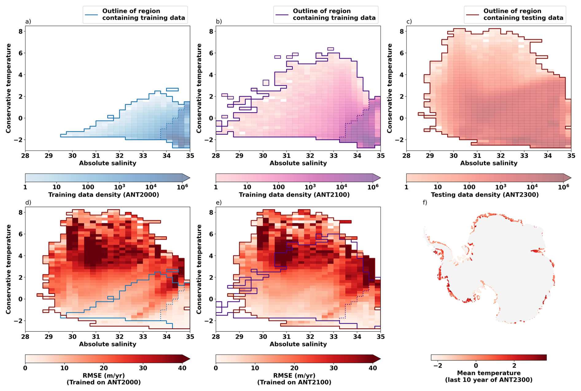
Figure 5 The highest RMSE values are observed for temperatures outside the range of the training dataset. The distribution of temperature and salinity for (a) the ANT2000 simulation, (b) the ANT2100 simulation and (c) the ANT2300 simulation. For ease of comparison, an outer contour is marked (solid line), and an inner contour bounding the region of highest data density (dotted line). (d) RMSE as a function of temperature and salinity when a neural network trained on the ANT2000 simulation is applied to the ANT2300 dataset. (e) RMSE as a function of temperature and salinity when a neural network trained on the ANT2100 simulation is applied to the ANT2300 dataset. (f) The mean temperature for the last 10 years of the ANT2300 dataset for each ice shelf grid point, showing that the highest temperatures are in basins such as B-C (Amery Ice Shelf) and F-G (Marie Byrd Land), where the neural network results in Fig. 4 were poorer.

In order to better understand the origins of mismatches between the predicted and reference sub-shelf melt rates, we look at the RMSE as a function of the neural network input variables. In particular, since these three simulations all have the same geometries, we look at RMSE as a function of conservative temperature and absolute salinity (Fig. 5), finding that the highest RMSE values occur when neural networks are applied to grid cells where the temperature is outside the range included in the training dataset for that neural network. The majority of data points in the ANT2000 simulation have a salinity between 33 and 35 g kg⁻¹, and a temperature between −2 and 1 °C. In the ANT2100 simulation, the majority of points have salinity between 32 and 35 g kg⁻¹ and temperatures between −2 and 2 °C. In contrast, in the ANT2300 dataset, salinities can be as low as 28 g kg⁻¹, and temperatures as high as 8 °C.

Interestingly, extrapolating to salinities which are outside the range included in the training dataset does not seem to pose as much of a problem as extrapolating to temperatures not included in the dataset (Fig. 5d and e). This is likely why the neural network trained on the ANT2000 simulation performs well when applied to the ANT2100 simulation (Fig. 3, RMSE = 110 Gt yr⁻¹), as the majority of grid cells have lower salinities but only marginally higher temperatures. There is also not a clear relationship between the mismatch to the training dataset and the error, suggesting that some of the other input variables also have an influence on RMSE. Despite these complex multivariate relationships, there is a clear need to include simulations with high temperatures in the training when looking to emulate future climate conditions.

3.3 Does the NN emulator work for different ice-shelf geometries?

The ANT2000, ANT2100 and ANT2300 simulations all have almost identical geometries, as the ice shelf draft is fixed and does not vary with time. However, in a coupled ocean-ice sheet model, the geometry would evolve. We therefore also consider data from a fourth simulation, ANTFGEOM, in which some ice shelves have had their geometry synthetically altered. This allows us to assess the impact of changes in geometry on the performance of the neural network.

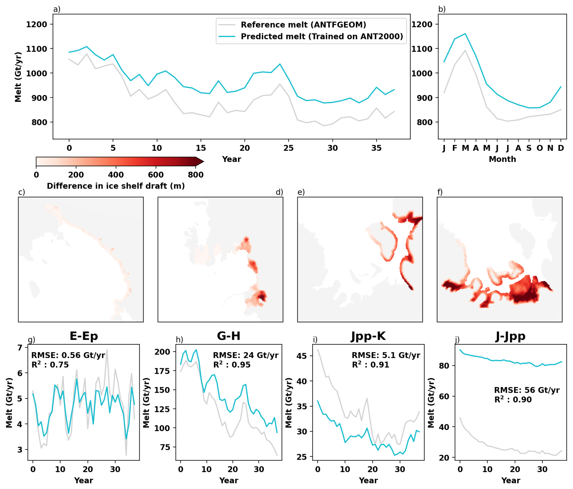
Figure 6 Neural network performance in a different geometry. The reference melt for the ANTFGEOM simulation (grey) and predicted melt for a neural network trained on the ANT2000 simulation (blue) either integrated over the whole of Antarctica (a, yearly, b, monthly), or for four of the 18 IMBIE basins. Panels (c)–(f) show the difference in the ice shelf draft for basins E-Ep (Ross Ice Shelf), G-H (Amundsen Sea), Jpp-K (Filchner) and J-Jpp (Ronne), which can be seen in more detail in Appendix A1. Panels (g)–(j) show the integrated melt rates for each of the four basins, and the root-mean-square error and correlation coefficient (R²) are given. Similar plots for all 18 basins can be seen in Fig. A2.

Figure 6 shows the results of applying a neural network trained on the ANT2000 data to the ANTFGEOM simulation. We find a good match between the integrated melt predicted by the neural network and the reference melt (Fig. 6, RMSE = 87 Gt yr⁻¹, R²=0.90), although the predicted melt is a slight overestimation. The ensemble spread is 5.31 Gt yr⁻¹ demonstrating that the parameter space is well constrained and all ensemble members give similar results.

To assess spatial patterns in the sub-shelf melt, we consider the melt integrated over each of the eighteen IMBIE basins. Melt rates for selected basins are shown in Fig. 6, and for all basins in Fig. A2a–r. There is significant variability in the quality of the ANT2000 neural network output when integrated on a basin scale. In particular, in the Ronne Ice Shelf (basin J-Jpp, Fig. 6j), the neural network melt prediction is nearly four times the melt rate from the reference ANTFGEOM simulation. If this single basin is removed from the integrated Antarctic melt, then the RMSE falls from 87 to 45 Gt yr⁻¹). Since the Filchner-Ronne Basin had the largest changes in geometry between the ANT2000 and ANTFGEOM simulations, it is not necessarily surprising that the largest errors are seen in this region, although we note that large geometry changes in the Amundsen Sea (basin G-H, Fig. 6h) and the Filchner Ice Shelf (basin Jpp-K, Fig. 6i) lead to only moderate errors.

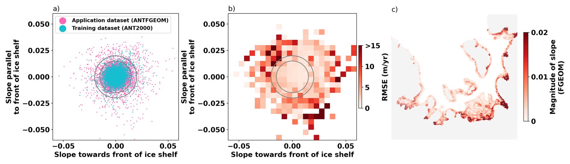
Figure 7 Average RMSE as a function of ice-shelf draft slope. (a) The distribution of data in the training dataset, ANT2000 (blue) and the ANTFGEOM simulation (pink), compared to (b) the RMSE as a function of the ice-shelf draft slope parallel (s_∥) and perpendicular (s_⟂) to the ice front when the neural network trained on the ANT2000 dataset is applied to the ANTFGEOM simulation. (c) The magnitude of the slope ($\sqrt{s_{⟂}^{\mathrm{2}}+s_{\parallel }^{\mathrm{2}}}$) of the ice-shelf draft in the Filchner-Ronne region in the FGEOM simulation. The grey circles show where the magnitude of the slope is 0.015 (inner) and 0.02 (outer) respectively.

In order to better understand the origins of these large errors, we look again at the RMSE as a function of the neural network input variables, focussing on the geometric inputs. Since the sub-shelf cavity was expanded in the ANTFGEOM simulation, there are some points much further from the grounding line than in the dataset used to train the ANT2000 neural network, which we might anticipate to be producing errors. However, analysis does not show any correlation between RMSE and the distance of a grid point to the grounding line or to the ocean. Instead, the geometric input variable with the strongest relationship to RMSE values is the slope of the ice-shelf draft, and we see the highest RMSE values in grid cells with steep slopes (Fig. 7b), which are particularly located very close to the grounding line. Since the ice shelf geometry was artificially thinning of the ice shelf for this NEMO simulation, the slopes in this region may be steeper than would be simulated in a coupled ice-ocean model.

In the training ANT2000 simulation, there are very few points with a slope higher than 0.015 (Fig. 7a). We see that when the ANT2000 neural network is applied to the ANTFGEOM simulation, the RMSE is highest where the slope exceeds 0.015 (Fig. 7b). The steepest slopes in the ANTFGEOM simulation occur in the Filchner-Ronne Ice Shelf (Fig. 6i and j), Amery Ice Shelf (Fig. A2d), and the Amundsen Sea (Fig. 6h), which are all regions where the neural network struggles to reproduce melt rates. The geometry was only altered a small amount in the Amery Ice Shelf basin between the two simulations, but the slope of the ice shelf draft there is at the very extreme of the values used in the training dataset, and so the neural network training is not optimised for such slopes.

We note that when a neural network trained on the ANTFGEOM simulation is applied to the ANT2000 dataset, and the ice shelf slopes are all within the limits of the training data, then the RMSE of the integrated melt is only 39 Gt yr⁻¹, or 4 % of the total integrated melt (not shown). It is therefore important that a neural network applied in a coupled simulation has been exposed to a range of slopes including steeper geometries in training.

3.4 Understanding neural network performance

In this manuscript we explore the performance of neural networks trained with limited data when applied to other simulations where we can verify the results against high resolution simulation melt rates. As expected, neural network performance is best when applied within the bounds of the training conditions, but we highlight that some input variables (temperature, slope of the ice shelf draft) seem to be particularly sensitive to extrapolation outside the training data. However, these neural networks are designed for use in the NEMO 1 degree ocean model, where we will not be able to verify the results against simulated melt rates. We therefore explore other indicators of neural network performance.

Ensemble spread can be used as an indication of the suitability of the neural network for the conditions in which it is applied. If the ensemble members have a large spread, this indicates that the parameter space has not been well covered during training, and that the random selection of the training and validation data has had a large influence on different ensemble members. Conversely, if the ensemble spread is small, then all ensemble members have converged on a similar solution, and the results are likely to be reliable.

Figure 8b shows the ensemble spread of a selection of neural networks when applied to the ANT2100 simulation. In general, high ensemble spreads are associated with high RMSE values. Sometimes, a high ensemble spread can be associated with a low RMSE, but we do not see any examples of a low ensemble spread and high RMSE value. Therefore, we provisionally suggest that if the ensemble spread is a significant fraction of the total integrated melt, then the neural network output should be considered with caution, and ideally more training data should be provided. However, this fractional threshold may vary depending on the nature of the input variable distributions in the training and application datasets.

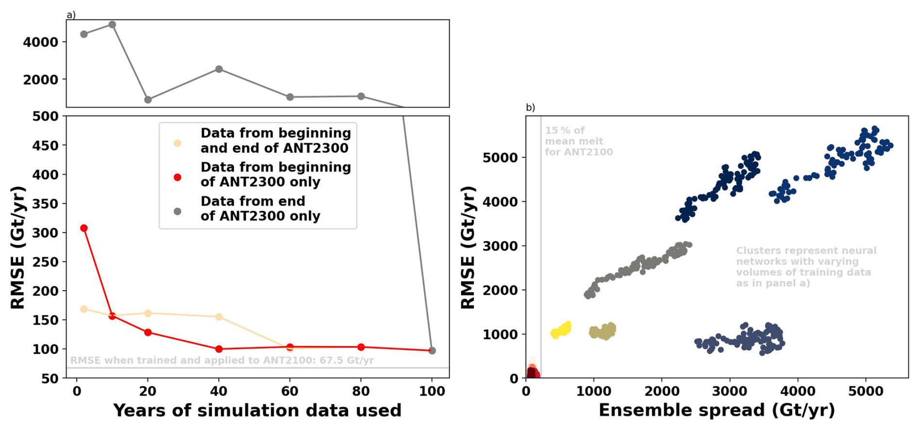
Figure 8 Neural network performance (RMSE) as a function of training data quantity, and ensemble spread. (a) The RMSE of the integrated reference melt from the ANT2100 simulation when compared to the predicted melt from neural networks trained with different volumes of data from the ANT2300 simulation. Results are shown when the selected data is either from the beginning of the ANT2300 simulation (red), both the beginning and end of the ANT2300 simulation (light orange), or the end of the ANT2300 simulation (grey, note that the break in the y axis at 500 Gt yr⁻¹, and that it resumes with different scale). The RMSE of the predicted melt from the neural network trained on the ANT2100 simulation and applied to the ANT2100 simulation is also shown in light grey (67.5 Gt yr⁻¹) as a comparison. (b) The RMSE of the integrated reference melt when compared to the ensemble spread (the standard deviation of the 10 neural networks). Each dot represents one year of data, and the coloured clusters are different simulations.

We also explore how much training data is required to achieve an acceptable neural network performance. We train neural networks with varying quantities of data from the ANT2300 simulation, and apply them to the ANT2100 simulation, as we know that a neural network trained on the whole ANT2300 performs well (Fig. 3, RMSE = 97 Gt yr⁻¹). Data is taken from either the beginning or the end of the ANT2300 simulation, or both. If 20 years of simulation data are used, this can either be 20 years from the beginning of the simulation (years 1–20), 20 years from the end of the simulation (years 81–100) or ten years from each of the beginning and the end (years 1–10 and 91–100). The results of applying these neural networks are shown in Fig. 8.

Firstly, we note that which part of the ANT2300 simulation the data is taken from has a significant effect on the results, and that neural networks trained only with data from the end of the ANT2300 simulation do not perform well, with extremely high RMSE values. As the end of the ANT2300 simulation represents conditions with significantly higher temperatures and melt rates that are never experienced in the ANT2100 simulation, this is not surprising. Even a neural network trained with the last 80 years of data from the ANT2300 simulation does not outperform a neural network trained on just the first 20 years of data. We therefore emphasise the need for training with appropriate data that are matched to the target simulation.

When we consider neural networks trained with only data from the beginning of the ANT2300 simulation, we see that increasing the amount of data included in the training improves the neural network performance up until about 40 years of data is used (RMSE = 99 Gt yr⁻¹). After this point, the RMSE of the simulation does not improve significantly. However, we note that the RMSE of neural networks trained with just 10 years of data is still only 157 Gt yr⁻¹, around 10 % of the total sub-shelf melt in this simulation. Although training with more data is better, we suggest that a minimum of at least 10 years of relevant simulation data is used in training when applying the neural network to new conditions.

4 Discussion

The neural network presented here produces melt rates that are closely correlated to the melt rates of the NEMO ocean model. This neural network architecture opens the door to a hybrid approach, where melt rates in some parts of the ice shelf are resolved with the full dynamics and thermodynamics of the ocean model, and melt rates in the remaining parts of these ice shelves or the entire cavity of small ice shelves can be calculated using the neural network. The output of the neural network is a map of sub-shelf melt rates, which can be integrated to give a total melt flux for use in an ocean model, or combined with melt rates from the ocean-model resolved region and fed directly into an ice sheet model. The neural network emulator can therefore be used in both stand-alone ocean simulations, or in coupled ocean-ice-sheet simulations.

Low resolution ocean models have started to be coupled to higher-resolution ice sheet models (Smith et al., 2021), but with unrealistic or no representation of melting in the smallest cavities and near the grounding line, which is thought to alter the simulated ice sheet dynamics. With coupled models that include the smallest cavities and the grounding zone, it will become possible to run long time-period simulations that include feedbacks between the ocean and the ice-sheet, such as evolving pinning points, changes in ocean stratification, and sea-ice production (Goosse et al., 2018; Li et al., 2024; Van Achter et al., 2023). This will be a significant improvement on models where the ice-ocean boundary is kept static and such feedbacks are neglected, especially as coupled regional models currently do not have a consensus on whether sub-shelf melt provides a positive or negative feedback to climate forcing (Seroussi et al., 2017; Timmermann et al., 2012; Pelle et al., 2021).

We provide as input variables for the neural network point-wise information about the cavity geometry and water properties as close to the cavity as possible. These input variables were chosen because they represent physical quantities which are known to impact sub-shelf melt rates and have been included in other parameterisations (Holland et al., 2008; Jourdain et al., 2020; Pelle et al., 2019; Lambert et al., 2023), including the whole ice-shelf neural network parameterisation of Burgard et al. (2023) which this work builds on. However, there are also additional variables that could have an impact on the sub-shelf melt rates, which are not included here. In particular, our NN considers local ocean conditions, and does not account for the horizontal circulation which should connect temperature and salinity properties between grid points, despite the importance of topography and Coriolis forcing in steering current through the ice-shelf cavity (Little et al., 2009; Gwyther et al., 2016). Within the point-wise neural network architecture, we suggest that in future work we could add information about the relative location of the grid point within the cavity or ice-shelf – possibly as simple as a −1 to 1 scale for left and right within the cavity. This may allow the neural network optimisation process to identify simple spatial biases in melt rate if they exist within the training data.

While considering the best neural network set-up, we considered other architectures alongside the point-wise perceptron employed here. Graphical neural networks are designed to accept sparse data on variable domains, and if employed here might have identified different relationships in the input data. However, in order to have good performance with a graphical neural network it is important to design the graph embedding structure correctly. The sub-shelf melt data does not have an obvious graph structure, and so it was unclear whether the additional complexity and expense of a graphical neural network would lead to any performance gains. Convolutional neural networks (CNNs) are widely used to identify patterns in image data, through the application of convolutional filters that consider relationships across multiple pixels. When applied to the parametrisation of sub-shelf melt, they could be used to identify drivers of melt at a wider spatial scale than is currently included. However, CNNs work best with a fixed input image size, and are less flexible for variable ice-shelf sizes (from 1 to 1368 grid points here) and resolutions than the point-wise architecture which we employ. For example, Rosier et al. (2023) used a modified U-Net CNN architecture (ResUNet$++$, Jha et al., 2019) as part of a two-step approach to predicting sub-shelf melt rates. However, their neural network was only trained on synthetic ice-shelves with a fixed image size, and did not demonstrate the adaptability of the point-wise neural network when it comes to applying to a range of real Antarctic ice-shelf geometries on both regular and irregular grids.

A potentially promising approach in the future may be to employ physics informed neural networks. These neural networks use physical laws to constrain neural network training, and have been applied to a wide range of problems in glaciology including studying the flow law of ice-shelves, and inverting for basal friction (Iwasaki and Lai, 2023; Cheng et al., 2025). When applied to the parameterisation of sub-shelf melt, similar thermodynamical constraints to the NEMO model could be used to maintain consistency and act as an additional regularisation factor. However, the physical equations used in NEMO and somewhat learned by the neural network should ensure some physical consistency in our approach.

It is important to note that the neural network emulator will only ever be as good as the NEMO model which is used to train it. Biases in the ocean model will be passed on in training and may be reproduced in the emulator, as we have seen with George VI ice shelf (Mathiot and Jourdain, 2023). Additionally, since we train with the NEMO 0.25° model as our “reference” melt rates, any processes that are neglected at this resolution in NEMO will also not be included in the emulator. This includes processes such as small-scale eddies, tidal fluctuations in the grounding line, melting in basal crevasses and boundary layer turbulence, which are known to influence melt rates beneath Antarctic Ice shelves from observations (Davis and Nicholls, 2019; Begeman et al., 2020; Washam et al., 2023) or model simulations (Richter et al., 2022; Patmore et al., 2023). However, since NEMO melt rates are tuned to be close to estimates from remote sensing, and temperatures and salinity are close to in-situ observations (Mathiot and Jourdain, 2023), some of these missing processes are implicitly accounted for in NEMO's parameter values. Additionally, one of the strengths of the emulator is that, should there be a significant update in the model physics which directly influences melt rates, relatively few higher-resolution simulations are required to retrain the emulator, which can then be rapidly employed in the low-resolution model. This approach can therefore save valuable computation resources while still facilitating the running of large ensemble coupled ice-sheet ocean models with realistic physics.

5 A neural network for application in the NEMO ocean model

We show here that a neural network can be used to emulate sub-shelf melt rates in the interior regions of ice shelves which are not resolved in the 1° NEMO ocean model, and that the neural network emulator performs best when trained in similar conditions to those which it is applied. In order to produce the most useful neural network for application in the 1° NEMO ocean model, we therefore additionally trained a neural network with all the available 0.25° simulations. We note that as we have trained this neural network with a wide range of temperature conditions, we would expect it to produce realistic melt rates for conditions similar to the present day and up to 2300. However, as we have trained limited variation in geometries and grounding line positions (2×155 basins), we would expect good performance in a model with a fixed grounding line, and would be more cautious about performance in an ocean model with evolving ice and bed geometries. To improve the generatlisation to changing geometries, we recommend adding simulations with different geometries and grounding line positions when available, and especially a larger range of ice-shelf slopes. Another approach could be to use synthetic ice-shelf geometries such as those used by Rosier et al. (2023) and upcoming high-resolution ocean-ice-sheet coupled simulations (e.g. De Rydt et al., 2024).

The resulting neural network is available in the package that accompanies this manuscript. As this emulator was trained with all the available simulations, there is no independent test data to verify the performance of this neural network. To provide an idea of the neural network performance we instead use the validation data set, which is used to tune the hyper-parameters used for training. When applied to the validation data set (11 % of the data points used in training), we report an RMSE of 3.29 m yr⁻¹ (ice equivalent), and a correlation coefficient R² of 0.93. As the validation dataset is selected randomly, metrics grouped by basin or year are uninformative. Based on these metrics, we expect this emulator to perform well when applied under conditions similar to the conditions in the training datasets. However, it will be necessary to do further model validation once the emulator is implemented in the 1° model to assess if it continues to reproduce the melt rates observed in the high-resolution model, as has been done in other studies including for parameterisations of convection (Yuval and O'Gorman, 2020) and vertical mixing (Zhu et al., 2022).

6 Conclusions

We demonstrate that sub-shelf melt rates within the interior segments of ice shelves not resolved in 1° global climate models can be emulated using a simple multilayer perceptron, and present a trained neural network which is ready for use in stand-alone ocean models or coupled ice-sheet-ocean models. This trained neural network leverages all the available continental 0.25° NEMO simulations to cover the maximum possible range of ice shelf conditions. We also explore the performance of neural networks trained with only selected simulations to understand how well the neural network generalises to new conditions. We show that these neural networks are quite sensitive to the range of input parameters, especially if applied to temperatures and ice-draft slopes outside those used in the training dataset. However, we find that the spread of the ensemble neural network results is a good indicator of the match between the training data and the conditions which the neural networks are applied in. If the ensemble spread is high relative to the total integrated melt (we suggest a threshold of >10 %), then this indicates that the training data was not suitable for this application, and ideally then additional simulation data would be provided. Our results show that as little as 10 years of targeted simulation data can improve the neural network performance. This manuscript is accompanied by python scripts that allow additional data to be added during neural network training. When trained with adequate simulations and employed in appropriate conditions, which can be verified with a suitable threshold on ensemble spread, the trained neural network presented here has the potential to significantly improve the representation of sub-shelf cavities in global ocean and climate models.

Appendix A

A1 Differences between simulations of ice-ocean conditions

Figure A1 shows the difference in geometries between the ANT2000 simulation and the ANTFGEOM simulation. The ANT2000 simulation uses the Bedmachine v2 (Morlighem et al., 2020) geometry, and the ANTFGEOM simulation is mostly identifical but has ice shelf draft is artificially thinned in the Amundsen Sea and Filchner-Ronne Ice Shelf regions following the MISOMIP2 protocol (De Rydt et al., 2024).

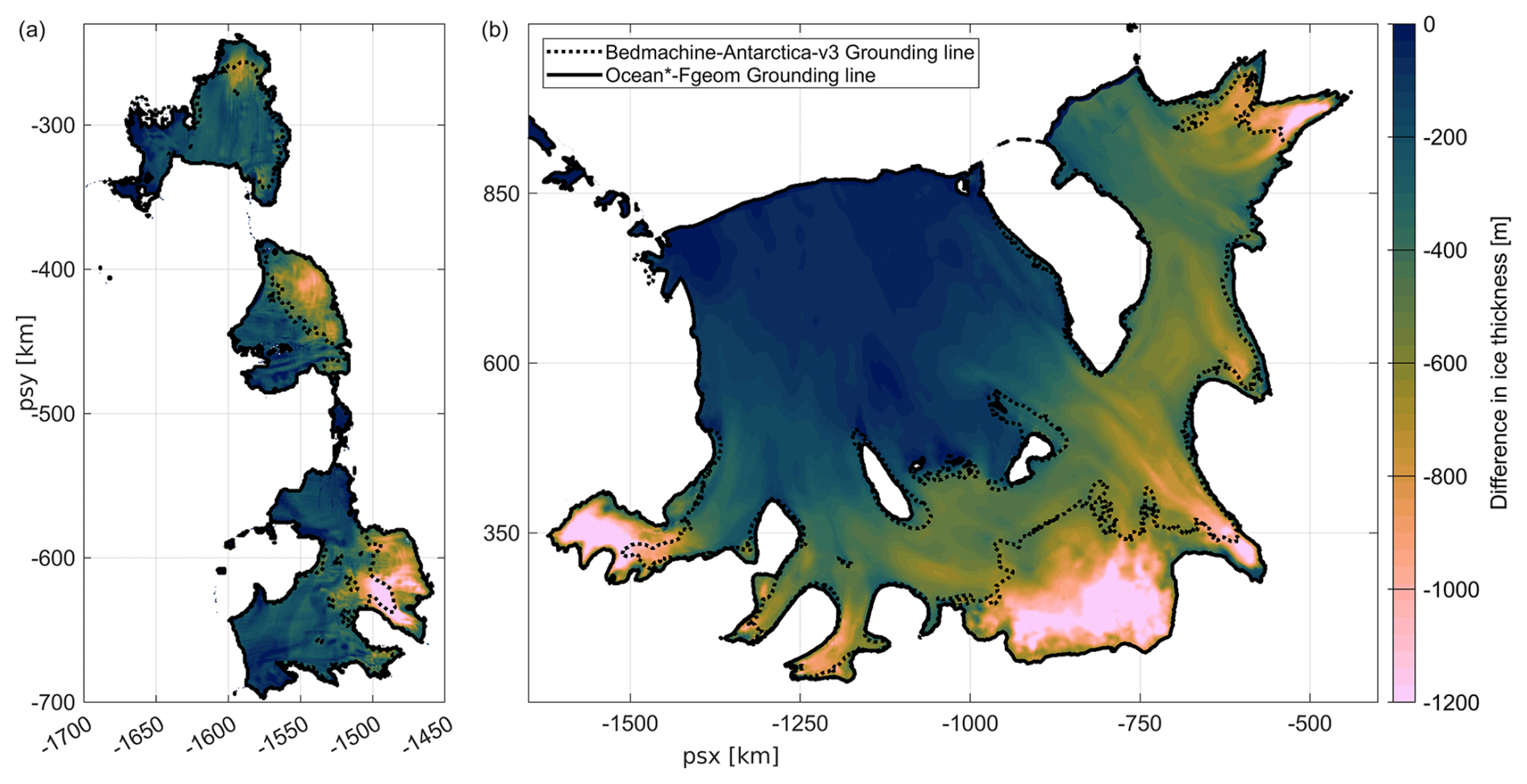
Figure A1 The difference in geometries between the ANT2000 simulation and the ANTFGEOM simulation. The ANT2000 simulation uses the Bedmachine v2 (Morlighem et al., 2020) geometry, and the ANTFGEOM simulation is mostly identifical but has ice shelf draft is artificially thinned in the Amundsen Sea (a) and the Filchner-Ronne Ice Shelf (b) regions following the MISOMIP2 protocol (De Rydt et al., 2024). Figure reproduced from De Rydt et al. (2024).

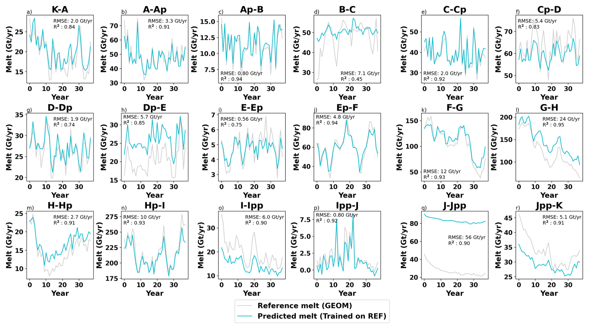
Figure A2 Neural network performance in a different geometry. The reference melt for the ANTFGEOM simulation (grey) and predicted melt for a neural network trained on the ANT2000 simulation (blue) for each of the 18 IMBIE basins (a–r). The root-mean-square error and correlation coefficient (R²) are given for each basin.

A2 Outlines of ice-shelf basins

In order to have a flexible framework which can adapt to evolving shelf geometries and changing grounding line positions, we divide the coastline of Antarctica into 155 partial ice-shelf basins, based on the locations of the individual outlet glaciers and ice streams (Fig. A3, Mouginot et al., 2017). Large pinning points (ice rumples and rises) are also separated and form their own basins. These basins are extrapolated into the open ocean using a nearest neighbour approach, and occasionally adjusted manually to ensure that basins which contain an ice-shelf front always have a few points in the open ocean. The resulting partial ice-shelf basins all have similar dimensions, with the exception of basins which include islands and are not part of the main coastline. The margins of the largest ice-shelves fall into several of these partial ice-shelf basins.

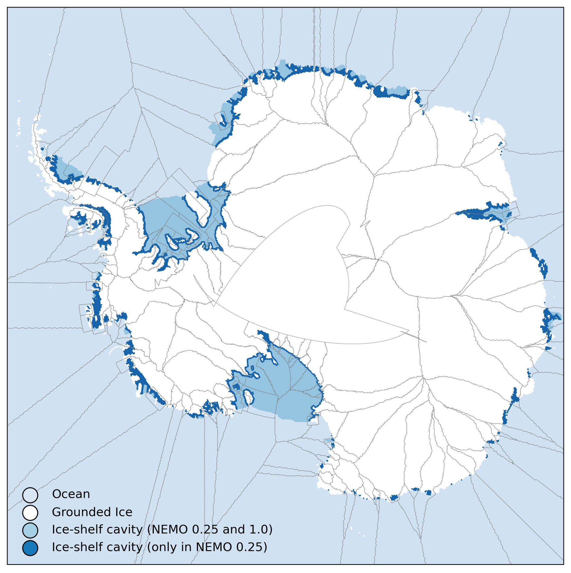
Figure A3 The outlines of the 155 partial ice-shelf basins, based on the locations of the individual outlet glaciers and ice streams (Mouginot et al., 2017), are shown by the light grey lines.

A3 Training with annual or monthly data?

Where available, we train the neural networks presented in the main body of the text with monthly data from each of the simulations. Neural network performance is improved by using monthly data, as shown in Fig. A4.

In order to assess the usefulness of training with monthly or annual data, we trained neural networks with data from the ANT2000, ANT2100 and ANT2300 simulations, with both annual and monthly data. Firstly, we consider the predicted melt rates from the ANT2000 and ANT2300 neural networks when applied to the ANT2100 simulation, which has intermediate temperature conditions slightly warmer than those in the ANT2000 simulation and cooler than those in the ANT2300 simulation. We expect that a neural network trained using monthly data should optimise the weights based on a wider range of temperature conditions, and would therefore return better results when applied to temperature conditions outside those in which it was trained. Indeed, our results show strongly reduced RMSE and higher correlation coefficients for neural networks trained using monthly data. For neural networks trained on the ANT2000 simulation, we see the RMSE fall from 200 to 110 Gt yr⁻¹ when monthly data is used instead of annual. For neural networks trained on the ANT2300 simulation, RMSE decreases from 130 to 97 Gt yr⁻¹. Therefore, we suggest that in order to maximise the training potential of a limited number of simulations, neural networks emulators of sub-ice shelf melt should be trained using monthly data wherever possible.

A4 Full metrics for simulations presented here

In addition to the metrics discussed in the main text, we report more comprehensive metrics for the main simulations presented here. In each case, a trained neural network is applied to the data from one of the NEMO simulations. We report the root-mean-squared error (RMSE) and correlation coefficient (R²) of the reference melt rate from the simulation compared to the melt rate predicted using the neural network. RMSE and R² are given for both the pointwise melt in m yr⁻¹ (ice equivalent) and for the integrated melt in Gt yr⁻¹. Integrated melt rates are given for the entire Antarctic continent, but also when melt is summed by basin.

Figure A5 shows metrics for the model validation experiments, when neural networks are applied to the same data that were used to train them. Figure A6 shows metrics for the testing experiments, when neural networks are applied to simulations which were not used in training to explore the performance of the neural networks in novel conditions. Finally, Fig. A7 shows metrics for the neural network which was trained on all the available simulations, when applied to each of these simulations.

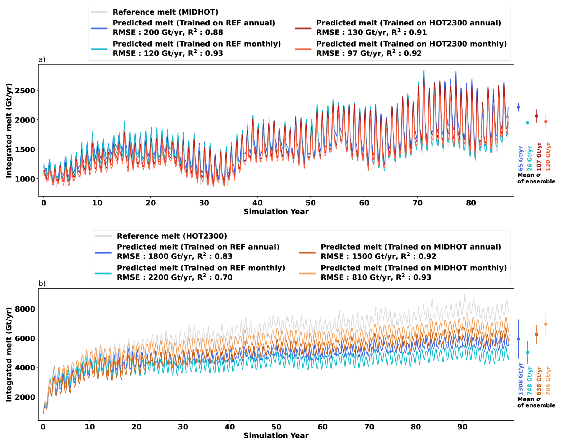
Figure A4 Should neural networks be trained with monthly or annual data? The results of applying neural networks trained on both annual and monthly data from ANT2000 and ANT2300 to the ANT2100 simulation, split into yearly (a) and monthly (b) trends. The reference melt rate for each simulation is show in grey. For all neural network predictions, the root-mean-square error (RMSE) in Gt yr⁻¹ and correlation coefficient (R²) are given in the legend.

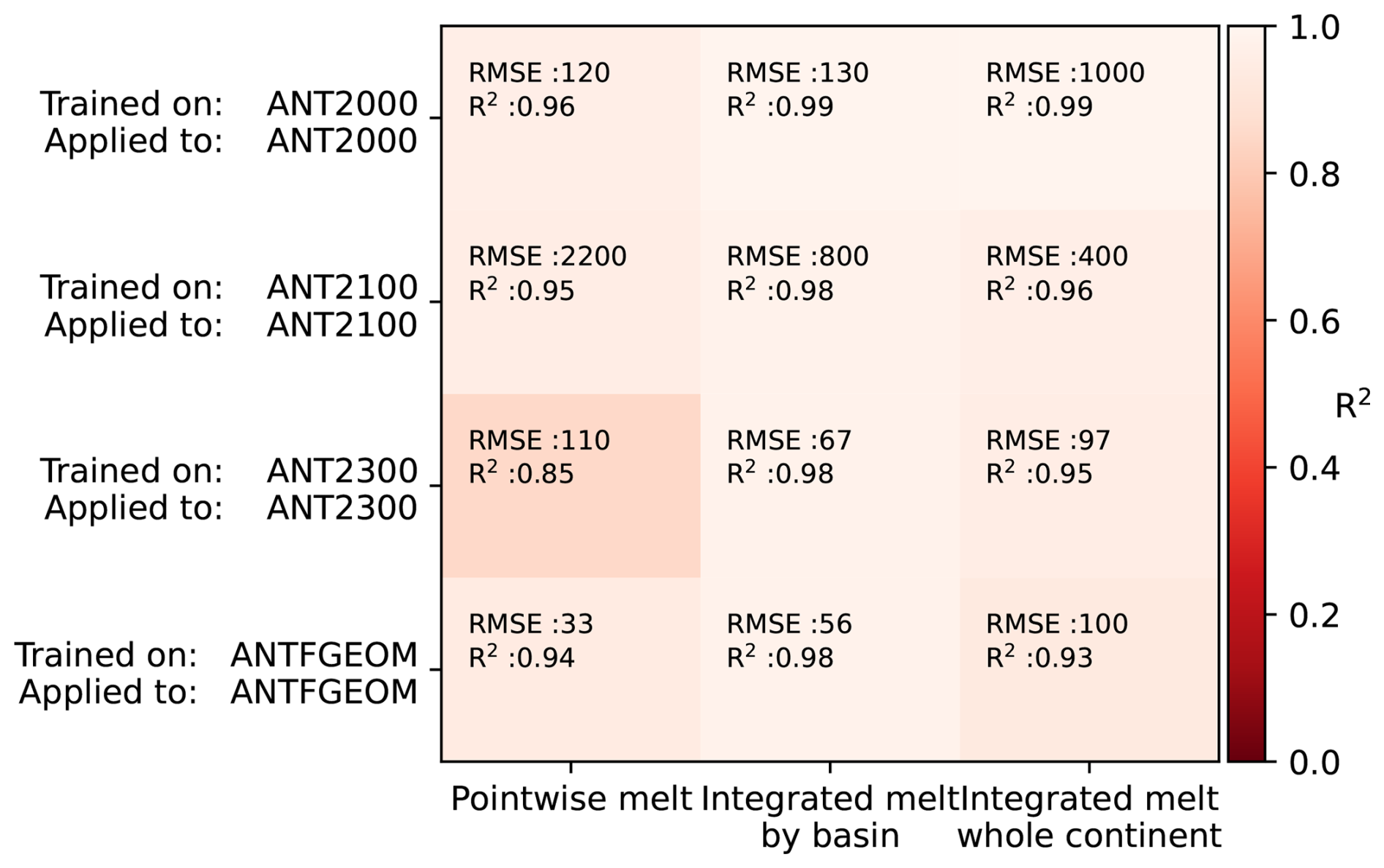
Figure A5 Metrics for the trained neural networks used in model validation. In each case, a trained neural network is applied to one of the simulations. We report the root-mean-squared error (RMSE) and correlation coefficient (R²) of the reference melt rate from the simulation compared to the melt rate predicted using the neural network, for the pointwise melt in m yr⁻¹ (ice equivalent) and for the integrated melt in Gt yr⁻¹ (integrated by basin and over the whole continent).

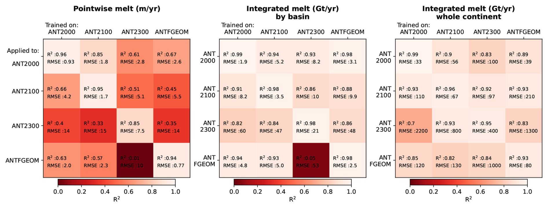
Figure A6 Metrics for the trained neural networks used in testing neural network performance. In each case, a trained neural network is applied to one of the simulations. We report the root-mean-squared error (RMSE) and correlation coefficient (R²) of the reference melt rate from the simulation compared to the melt rate predicted using the neural network, for the pointwise melt in m yr⁻¹ (ice equivalent) and for the integrated melt in Gt yr⁻¹ (integrated by basin and over the whole continent).

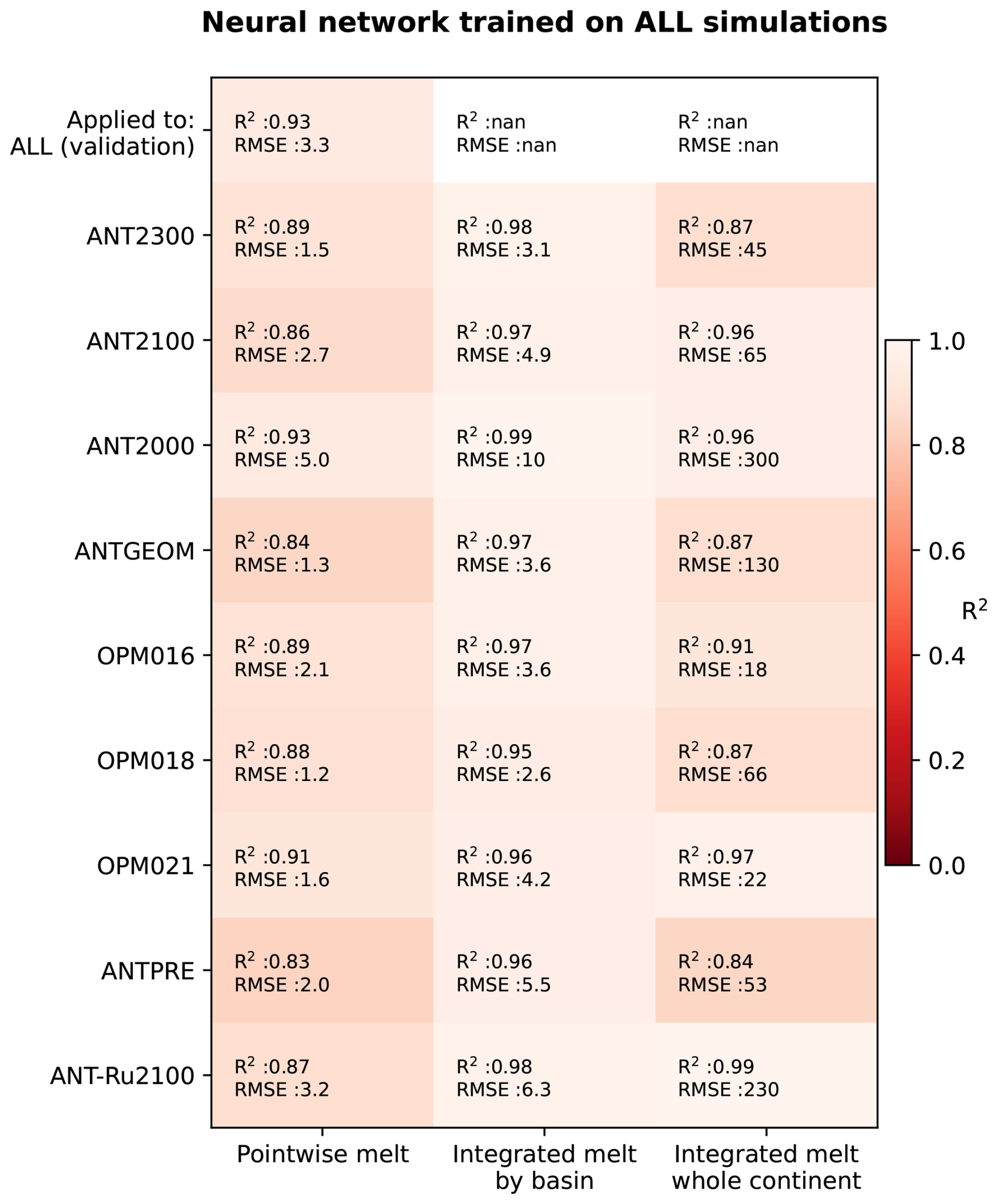
Figure A7 Metrics for neural networks trained using all available NEMO simulations. The neural network is trained with all available simulations, and then applied to each one, as well as to the validation data set from the training. We report the root-mean-squared error (RMSE) and correlation coefficient (R²) of the reference melt rate from the simulation compared to the melt rate predicted using the neural network, for the pointwise melt in m yr⁻¹ (ice equivalent) and for the integrated melt in Gt yr⁻¹ (integrated by basin and over the whole continent).