Ensemble forecasts of isolated and compound wind and precipitation extremes in Europe using HC-SWG (v3.1) and MA-SWG (v1.1) Stochastic Weather Generators

Ensemble forecasts of extreme wind and precipitation provide essential information for early warning systems. In this study, we present two forecasting approaches that combine a stochastic weather generator (SWG) with atmospheric circulation analogs to forecast extreme precipitation and extreme wind speed in Europe. The first approach, which we term HC-SWG, combines ECMWF ensemble reforecasts with the stochastic weather generator to forecast extreme precipitation at different locations in Europe. The second approach, which we term MA-SWG, uses multivariate atmospheric analogs as input to the SWG to forecast extreme 10 m wind speed. These ensemble forecasts of precipitation and wind speed extremes display a higher forecast skill than ECMWF numerical reforecasts at lead times up to 10 d, using station data as the ground truth. As a final step, we evaluate the forecasted and observed frequencies of simultaneous and sequential precipitation and wind speed extremes in Europe, which are a class of high-impact compound events. Our forecasts yield comparable occurrence frequencies to the observations.

1 Introduction

The isolated or compound occurrence of wind and precipitation extremes can result in large detrimental impacts on natural and socio-economic systems. Examples include ecosystems, agricultural production, and industry (Hao et al., 2022; Weinkle et al., 2018; Zscheischler et al., 2020). Wind and precipitation extremes can also cause fatalities and property losses, for example, through extreme waves, storm surges, and flooding in low-lying coastal areas (Fang et al., 2021; Bevacqua et al., 2019). Improving the forecast of these and other extreme weather events, particularly at the medium range (1 to 10 d), is essential for issuing timely early warnings (Vitart et al., 2019).

Numerical weather prediction (NWP) models, based on a process-based modelling of the evolution of the atmosphere, have until recently been the dominant approach for weather forecasting (Magnusson et al., 2023). Their performance has improved in the last decades thanks to more accurate initial conditions and parametrisations and higher resolution (Ben Bouallègue et al., 2019; Vitart et al., 2019; White et al., 2022). Recently, data-driven forecasting models have achieved comparable or better skill than NWP models (Bouallègue et al., 2024; Rasp et al., 2024).

However, both NWP and data-driven models face challenges in accurately forecasting extreme events (Haiden et al., 2023; Ben-Bouallegue, 2023; Domeisen et al., 2022). For instance, Olivetti and Messori (2024) highlighted the limitations of data-driven models in predicting cold extremes and noted significant regional variations in the forecast skill of different data-driven models. They ascribed this in part to the fact that the models are optimised for overall forecast skill at the cost of comparatively poorer performance for extreme events. The limitations of NWP arise from its constrained ability to resolve small-scale processes that influence meteorological variables such as precipitation or near-surface wind speed. Although substantial progress has been made in the parameterization of subgrid-scale phenomena, significant uncertainties remain within these schemes (Hersbach et al., 2020; Haiden et al., 2023). Another major challenge lies in the initialization of variables: while large-scale atmospheric fields can be accurately initialized using satellite and radiosonde observations, the initialization of surface variables is often hindered by data quality and incomplete global coverage of in situ surface data (Haiden et al., 2023). These challenges are compounded by the high computational costs associated with producing numerical forecasts at very high spatial resolution. This requires either high-resolution global models, or post-processing and downscaling to obtain high-resolution regional forecasts (Ben Bouallègue et al., 2023; Specq and Batté, 2020; Stevens et al., 2019; Alessi and DeGaetano, 2021). The latter significantly enhances forecast accuracy at local scales and for some challenging weather variables such as precipitation and wind. Machine learning or statistical techniques can also be combined with NWP models to correct forecast biases, downscale the forecasts and enhance forecast quality (Ben Bouallègue et al., 2023; Specq and Batté, 2020; Harris et al., 2022).

An alternative approach to NWP and data-driven models comes from stochastic weather generators (SWGs). These can be used as a forecasting tool or as a postprocessing tool, and can generate very large ensembles at a low computational cost (Ailliot et al., 2015; Yiou and Déandréis, 2019; Yiou, 2014; Brunner et al., 2021). SWGs have also been combined with circulation analogs – namely sets of similar states of the atmospheric circulation. This combined tool showed promising forecast skill for variables such as precipitation and temperature (Krouma et al., 2022, 2024; Atencia and Zawadzki, 2017; Blanchet et al., 2018) at subseasonal lead times of 25 to 30 d, as well as in forecasting climate indices such as the North Atlantic Oscillation and the Madden Julian Oscillation (Krouma et al., 2023; Yiou and Déandréis, 2019).

In this study, we aim to use a SWG to produce ensemble forecasts of local extreme precipitation and wind speed events in Europe. We use two different forecasting approaches for the two variables. For extreme precipitation, we combine the SWG with the European Centre for Medium-Range Weather Forecasts (ECMWF) ensemble reforecasts (also known as hindcasts, or HC). This approach, which we term HC-SWG, uses analogs from the reforecasts, defined using 500 hPa geopotential height. It was tested in Krouma et al. (2024) to forecast subseasonal precipitation in Europe. Here, we apply it specifically to precipitation extremes. For extreme wind speed, we adopt the MA-SWG based on multivariate atmospheric analogs (MA). We developed the MA-SWG specifically to forecast the wind speed, after finding that analogs computed using a single atmospheric variable provided limited forecast skill for wind extremes.

The rest of the paper is structured as follows: Sect. 2 details the data used in our forecasts. Section 3 describes the forecasting process, including the circulation analogs computation and the two different versions of the SWG, and explains the verification metrics used to evaluate the forecast skill. The evaluation of the SWG ensemble forecasts, and their comparison to the ECMWF forecasts for precipitation and wind speed extremes as well as the compound forecast evaluation, are presented and discussed in Sect. 4. Section 5 outlines the main conclusions.

2 Data

We use daily data for precipitation and wind speed retrieved from the European Climate Assessment and Data (ECA&D) project for 9 locations across Europe (Bergen, Berlin, Brest, De Blit, Linköping, Madrid, Orly, Santander, and Stockholm) (Klein Tank et al., 2002) from 1960 to 2022. The choice of those locations was based on: (i) ensuring diversity of meteorological conditions; and (ii) the availability of co-located observational data for precipitation and wind speed. The ECA&D data is used as ground truth.

We also use ERA5 reanalysis data (Hersbach et al., 2020), with a resolution of 0.25° × 0.25° over 1960 to 2022. Hourly geopotential height at 500 hPa (Z500) and Sea Level Pressure (SLP) were used to obtain daily data over the region of 80° W–40° E, 30–90° N. We consider this geographical domain to cover all the different analysis locations and to optimise computation time. For investigations focusing on specific locations or small regions, targeted domains could instead be used.

We further analyse reforecasts of Z500 collected from the ECMWF subseasonal to seasonal (S2S) database (Vitart et al., 2017) over the region of 80° W–40° E, 30–90° N. The ECMWF reforecasts comprise an 11-member ensemble covering the past 20 years, and running up to 46 d lead time (Vitart et al., 2019). As initial conditions, the reforecasts use ERA5 and ORAS5 for the atmosphere and ocean, respectively. We consider the ensemble members at different lead times δ from 1 to 5 d. We chose the model version CY47R3, available from 2001 to 2021, with a horizontal resolution of 15 to 31 km and providing daily data, which contains ice and ocean initial conditions (Vitart et al., 2019).The ERA5 and S2S data are used to define analogs of the atmospheric circulation.

Finally, we considered ECMWF forecasts of precipitation and u and v components of 10 m wind from the THORPEX Interactive Grand Global Ensemble (TIGGE) database from 2017 to 2021 (Bougeault et al., 2010). We used the TIGGE database to evaluate our SWG forecasts, as it provides actual operational ensemble forecasts issued daily in near-real-time, with higher spatial resolution (9 km) and more frequent initialisations (daily as opposed to bi-weekly) than the S2S database (Bougeault et al., 2010). This makes them ideal for verifying medium-range forecasts of extreme precipitation and extreme wind speed. The forecasts (referred to in the rest of the paper as ECMWF forecasts) for wind and precipitation have been bias-corrected. For comparison to the SWG forecasts, we considered ECMWF forecast data at the closest gridded points to the geographical coordinates of the studied stations as indicated in ECA&D.

We define extreme precipitation and extreme 10 m wind speed as the precipitation (wind speed) that exceeds the empirical local 95th percentile from the ECA&D data. For precipitation, the percentile was computed after excluding values below 1 mm d⁻¹. From the ECMWF forecasts, the same definition was applied, but using the 95th percentile of the climatological forecast distribution.

3 Methods

3.1 Forecasting tools: Analogs & SWG

To forecast precipitation and wind speed extremes over Europe, we leverage analogs of the atmospheric circulation and SWGs. Here, we describe two configurations of the SWG. For extreme precipitation, we use the HC-SWG (Sect. 3.1.1), previously tested to forecast sub-seasonal precipitation by Krouma et al. (2024). HC-SWG combines the stochastic weather generator with NWP reforecasts. For extreme wind speed, we use the MA-SWG (Sect. 3.1.2), namely a stochastic weather generator combined with multivariate atmospheric analogs.

3.1.1 Extreme Precipitation forecast approach: HC-SWG

We use the ECMWF S2S ensemble reforecasts at lead times of δ=1 to 5 d to forecast extreme European precipitation (Fig. 1). We first look in the ensemble reforecasts initialised at time t₀ and with lead time δ for analogs of the Z500 on a target date t_0+δ. We define analogs based on Euclidean distance, and consider only dates within a calendar window of 30 d around the date of t_0+δ yet in different years than t_0+δ. We then keep the K=20 best analogs for each target day t_0+δ.

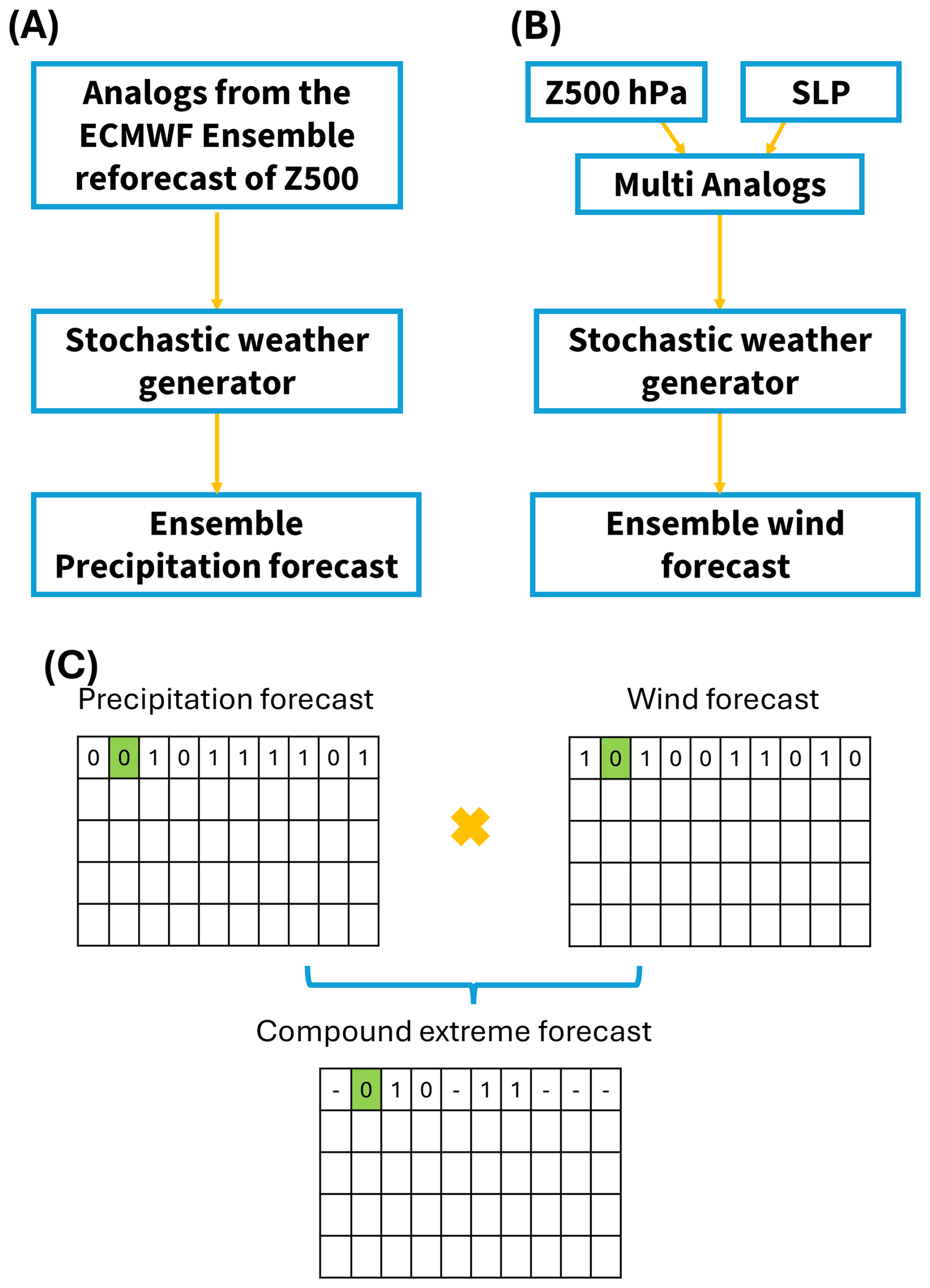
Figure 1 Illustration of the forecast process. (a) The HC-SWG used to forecast extreme precipitation; (b) the MA-SWG used to forecast wind speed, and (c) the ensemble forecast of the co-occurrence of precipitation and wind speed extremes.

We next produce forecasts by generating random trajectories based on the identified analogs, following the procedure outlined in Krouma et al. (2024). The initialization point of our forecasts is set at t_0+δ, and each trajectory extends to time $t_{\mathrm{0}+\mathit{\delta }}+T$, with the lead time T ranging from 1 to 10 d. Beginning on day t_0+δ, we randomly select an analog $t_k^{\prime }$ among the K=20 best analogs. The random selection of analogs of the day is carried out using weights that are proportional to the calendar difference between t_0+δ and the analog dates, in order to ensure that time progresses (Yiou, 2014). We then replace t_0+δ with the selected analog of $t_k^{\prime }$ and repeat the operation T times.

The above process produces a random trajectory between t_0+δ and $t_{\mathrm{0}+\mathit{\delta }}+T$. The procedure is repeated to simulate N=100 trajectories, providing an initialised ensemble forecast. The SWG reforecasts are started every Δt≈ $T/\mathrm{2}$ d between 1 January 2002 and 31 December 2021 (Fig. 1a). The daily precipitation of each trajectory is time-averaged between t_0+δ and $t_{\mathrm{0}+\mathit{\delta }}+T$. Hence, we obtain an ensemble of N=100 forecasts of average precipitation over T days. From these average precipitation values, we define extremes as values in excess of the 95th percentile of the distribution for the full forecast period. The HC-SWG in this paper has been improved compared to Krouma et al. (2024) by defining analogs from the full ECMWF ensemble reforecast of Z500 compared to the use of the ensemble reforecast mean in Krouma et al. (2024). We additionally test the sensitivity of the HC-SWG forecast to δ instead of using a fixed δ value (Appendix D).

We illustrate the procedure with an example, where we generate an ensemble forecast of extreme precipitation starting on t₀ = 20 February 2020, with a forecast lead time T=6 d, which is the 26 February 2020. We set δ=5 d, so our starting point is the Z500 reforecast initialised on the 20 February 2020 and with a lead time of 5 d, corresponding to t_0+δ = 25 February 2020. As first step, we identify the K=20 best analogs of the Z500 field on 20 February (within a ±30 d calendar window, excluding dates in 2020), and randomly select one analog weighted by calendar date similarity – for example, 23 February 2011. We repeat this process for 23 February 2011. We take the reforecasts initialised on 23 February 2011, with lead time δ = 5 d, and find the K=20 best analogs for 28 February 2011 (excluding dates in 2011) and select one randomly – for example, 2 March 2008. We continue this iterative process until we have a timeseries of 6 dates. For each step t_k, we use the Z500 field to estimate daily extreme precipitation. We then calculate the mean precipitation over these 6 d to produce one forecast: the average of precipitation over 20 to 26 February 2020. This entire procedure is repeated N=100 times, each time generating a different random analog sequence, to create an ensemble of 100 forecasts of precipitation for the period 20–26 February 2020.

3.1.2 Extreme Wind forecast approach: MA-SWG

The multivariate analogs SWG relies on analogs computed using daily averages of Z500 and SLP from ERA5 reanalysis data (Fig. 1b). These variables provide information on both the mid-tropospheric and surface large-scale circulation (Buizza and Leutbecher, 2015). We also tested adding the Z250 as a third variable, but found that this degraded our forecast skill.

We first compute Empirical Orthogonal Functions (EOFs) from anomalies of Z500 and SLP, analysing the two separately. The anomalies are defined relative to the daily mean climatology over the period from 1960 to 2022. We apply a cosine-of-latitude weighting during the EOF analysis to account for grid-area variations. We keep the s principal components that contain at least 90 % of the variance (s=6 for Z500, and s=10 for SLP). Therefore, we have 16 daily time series from 1960 to 2022 corresponding to the selected principal components. Analogs for each target day are computed from this timeseries data, finding the closest tuples of values to the tuple of the target day. We again consider a window of 30 calendar days around the target day and exclude analogs in the same year as the target day. Then, we generate ensemble forecasts of wind speed using these analogs, following the same procedure described for the HC-SWG (Sect. 3.1.1). The difference is that in the MA-SWG we do not use reforecast data, and hence there is no δ. We again average the wind speed over the forecast lead time.

We take as example an initialization date t₀ = 20 February, 2020 and a forecast lead time T=6 d. As a first step, we find the K=20 best analogs of t₀ in the principal component space, and select one randomly (weighted by calendar difference), for example, 22 February 2011. We next repeat this process iteratively to generate the rest of the trajectory up to T days. We then compute the average wind speed over the forecast period and repeat the whole process N=100 times to produce an ensemble of 100 forecasts of average wind speed between 20 and 26 February 2020.

3.2 Compound extreme forecast

We based the compound extreme forecast of wind speed and precipitation in the 9 studied locations on the ensemble forecasts generated from the HC-SWG and the MA-SWG (Fig. 1c). To do so, each forecast ensemble is represented as a grid of binary values. A value of “1” was assigned when the majority of ensemble members in the forecast display an extreme event, while a value of “0” was assigned when the majority did not indicate an extreme event (Sutanto et al., 2020). The compound extreme forecast is derived by identifying overlapping occurrences of extremes in both precipitation and wind speed ensembles. We also checked the cases of sequential extremes, namely extreme precipitation events and extreme wind speeds occurring in succession within lags of 1 to 5 d of one another.

3.3 Forecast Evaluation

We evaluate the ability of the HC-SWG and MA-SWG to forecast extreme precipitation and wind speed, respectively, by using the Symmetric Extremal Dependence Index (SEDI) and the Peirce Skill Score (PSS). These two metrics are particularly suited for rare events (Ferro and Stephenson, 2011; Magnusson et al., 2014; Stephenson et al., 2008a). Unlike traditional scores, they emphasise event discrimination and forecast skill under low base-rate conditions and are less influenced by class imbalance, thus providing a more reliable assessment of the model's ability to detect extremes (Stephenson et al., 2008a).

The SEDI accounts for hits (H), false alarms (F), misses (M), and correct rejections (C), and is defined as:

$$\begin{array}{}\text{(1)}& \mathrm{SEDI}={\displaystyle \frac{\log (H/M)-\log (F/C)}{\log (H/M)+\log (F/C)}}.\end{array}$$

We assessed forecast skill beyond random chance using the PSS (Stephenson, 2000; Manzato, 2007). The PSS ranges from 0 to 1, where PSS=1 corresponds to a perfect forecast, and PSS=0 indicates that the forecast performs no better than random chance. We calculated the PSS as:

$$\begin{array}{}\text{(2)}& \mathrm{PSS}=\mathrm{POD}-\mathrm{FAR},\end{array}$$

where POD is the Probability of Detection and FAR is the False Alarm Ratio, which in this context is sometimes referred to as POFD (Probability Of False Detection) in the literature.

The FAR measures the frequency of false alarms relative to the total number of forecasted extreme events, while the POD quantifies the fraction of observed extreme events that were correctly forecasted. These metrics are defined as:

$$\begin{array}{}\text{(3)}& {\displaystyle }\mathrm{FAR}={\displaystyle \frac{F}{H+F}},\text{(4)}& {\displaystyle }\mathrm{POD}={\displaystyle \frac{H}{H+M}}.\end{array}$$

High values of POD and FAR indicate overprediction of extremes, low values of POD and FAR suggest missing extremes, and high values of POD with low values of FAR indicate good forecasting skill (Wilks, 2011). We compute SEDI and PSS considering different thresholds, the 20th, 70th, and 90th quantiles of the distributions of extreme precipitation (and extreme wind speed), to evaluate the ability of the HC-SWG (MA-SWG) to forecast the most extreme values of the extreme precipitation (wind speed extremes).

Finally, we compared the ensemble forecasts of the HC-SWG and the MA-SWG to the ECMWF ensemble forecast using the Brier skill score (BSS). The BSS is computed between the Brier score (see Appendix C) of the HC-SWG (MA-SWG) forecast and the Brier score of the ECMWF precipitation (wind speed) forecast, which we consider as a benchmark, as follows:

$$\begin{array}{}\text{(5)}& \mathrm{BSS}=\mathrm{1}-{\displaystyle \frac{{\mathrm{BS}}_{\mathrm{SWGs}}}{{\mathrm{BS}}_{\mathrm{ECMWF}}}}.\end{array}$$

Values above 0 indicate that the SWG forecasts are better than ECMWF forecasts; a value of zero indicates equal performance of the different forecasts, and negative values indicate that the ECMWF forecasts outperform the SWG forecasts (Hersbach, 2000).

To investigate further the difference between the SWGs forecasts and the ECMWF forecasts, we compute the cumulative distribution functions (CDFs) of both the SWG and ECMWF ensemble forecasts.

4 Results

4.1 Evaluation of the extreme precipitation forecasts

We evaluate the HC-SWG's forecasting skill for extreme precipitation over Europe. We focus here on the results using δ=5 d. Results showing the sensitivity of the forecast performance to different δ are provided in Appendix D.

The HC-SWG reproduces closely the time series of the observed extreme precipitation amounts from 2002 to 2021 at lead times of up to 10 d. Figure 2 shows the results for Linköping (Sweden). The HC-SWG forecasts are particularly good for the moderate extreme events, while they display an overestimation of the most extreme precipitation values (upper tails in Fig. 2b, d, f). This behavior is likely linked to the stochastic nature of the HC-SWG, which may require further calibration to refine its ability to predict the highest extreme precipitation values accurately. As the lead time T increases, the amplitude of both the observed and forecasted extreme precipitation events decreases. Indeed, longer forecast horizons imply averaging extreme precipitation across more days, and thus lead to a smoothing effect.

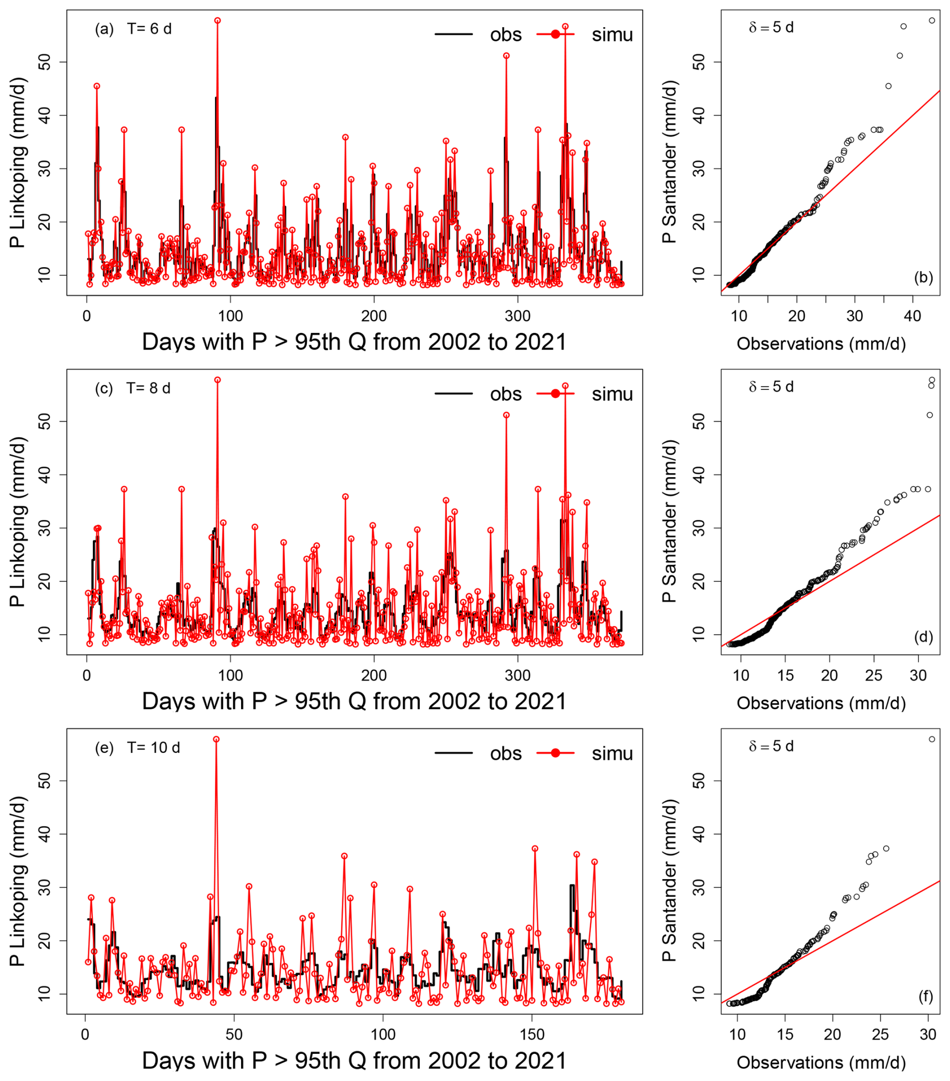
Figure 2 Comparison of observed and forecasted extreme precipitation events using the HC-SWG at lead times T=6, 8 and 10 d for Linköping. Panels (a), (c), (e) display observed (black) and forecasted (red, defined as the median of the 100 members) mean extreme precipitation values (mm d⁻¹) from 2002 to 2021. Panels (b), (d), (f) present scatter plots comparing observations and forecasts, with the red diagonal lines representing a perfect 1 : 1 relationship.

The other stations that we consider present results in line with those for Linköping (Fig. 3). We again find a strong forecast performance for moderate extreme events and widespread overestimation for the most extreme events, with the discrepancy growing larger at longer lead times (Fig. 3). There is some variability across stations, with some (e.g. Bergen) displaying larger forecast errors while others (e.g. Berlin) display better agreement. Nonetheless, the qualitative overestimation pattern for the most extreme events is similar across all stations.

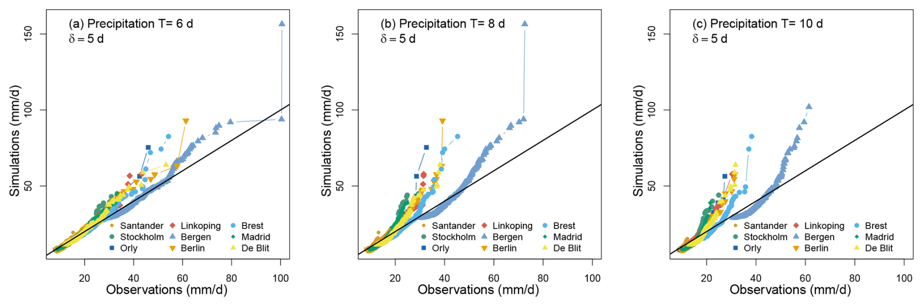
Figure 3 Comparison of observed and forecasted extreme precipitation events using the HC-SWG at lead times T=6 (a), 8 (b) and 10 (c) days for all stations considered here. The panels present scatter plots comparing observed and forecasted extreme precipitation values (mm d⁻¹) from 2002 to 2021 on days exceeding the local 95th percentile. The black diagonal lines represent a perfect 1 : 1 relationship.

Overall, the results illustrate the ability of the HC-SWG to accurately forecast heavy precipitation events at medium-range timescales, with some variations in performance across different stations and a clearly degraded performance for the most extreme events.

To quantify the performance of the HC-SWG forecasts, we compute the PSS and SEDI for different quantiles of extreme precipitation going from the 20th to the 90th quantiles (Fig. 4). PSS quantifies the added value of the HC-SWG forecasts compared to a random forecast. For all stations, PSS remains close to one across all the percentiles and lead times (Fig. 4a, c, e). Indeed, the forecasts have relatively low FAR and relatively high POD, resulting in high PSS values and indicating a good forecast skill. The forecasts display a relatively stable PSS for moderate (exceeding the 70th quantile of the distribution of extreme precipitation) and most extreme events (exceeding the 90th quantile of the distribution of extreme precipitation) for different lead times. This indicates that the HC-SWG retains a strong ability to correctly distinguish between exceedance and non-exceedance events even at longer lead times. The weak decrease in PSS with lead time also suggests that the HC-SWG is robust in terms of event detection.

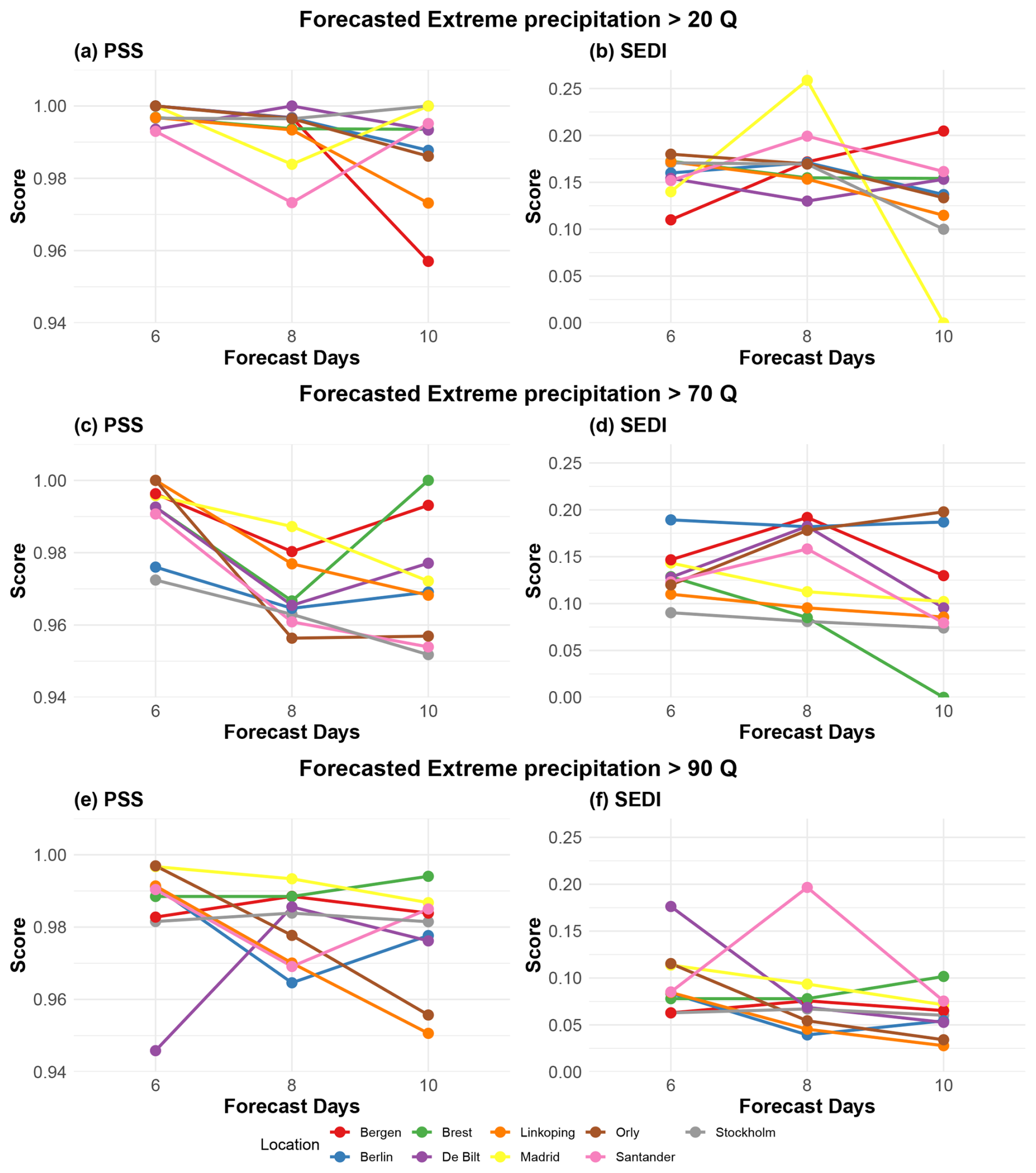
Figure 4 Extreme precipitation forecast skill for HC-SWG evaluated using PSS (a, c, e) and SEDI (b, d, f) at lead times T=6, 8 and 10 d for all stations considered here. We consider separately events above the 20th, 70th and 90th quantiles of the extreme precipitation days (i.e. > 95 Q of the full distribution).

SEDI accounts for hits, false alarms, misses and correct rejections. There is a slight degradation of performance with increasing lead time, but this is highly variable across stations, with a number of stations showing higher SEDI values at longer lead times (Fig. 4b, d, f). SEDI values remain relatively positive even for the most extreme events. Indeed, even though the magnitude of these events is overpredicted in the forecasts, they qualify as exceeding a given quantile in both the forecasts and observations, and thus do not count as false alarms. Compared with PSS, SEDI reveals a clearer station dependence, with a larger spread across locations, especially for the highest threshold. This suggests that although the HC-SWG performs well overall, its skill in forecasting rarer events is not spatially uniform. For the 90th quantile in particular, the larger spread across stations points to station-dependent differences in predictability or model performance for the most severe precipitation extremes. Nevertheless, the fact that SEDI remains positive for nearly all stations and lead times confirms that the forecasts retain useful skill even under a stricter rare-event metric.

These results again indicate a strong forecast performance of the HC-SWG, albeit with some lead-time and location dependence.

We next compare the HC-SWG ensemble forecast of extreme precipitation to the ECMWF forecasts for the 9 studied stations using the BSS at different lead times T (Fig. 5). The BSS values are between 0.4 and 0.98 for all lead times going from 6 to 10 d, which indicates that HC-SWG outperforms ECMWF forecasts for extreme precipitation. The BSS values decrease with lead time and are spatially dependent. This confirms that the added value of HC-SWG over ECMWF is robust across all stations, although the magnitude of the improvement varies substantially from one location to another. Some stations such as Santander, Stockholm and Berlin maintain very high BSS values even at day 10, whereas others, mainly Madrid and Orly, show a more marked decrease with lead time, indicating that the benefit of the stochastic approach is stronger in some local precipitation regimes than in others. Still, the consistently positive BSS values indicate that HC-SWG provides an improvement over ECMWF even at the longest lead times considered here.

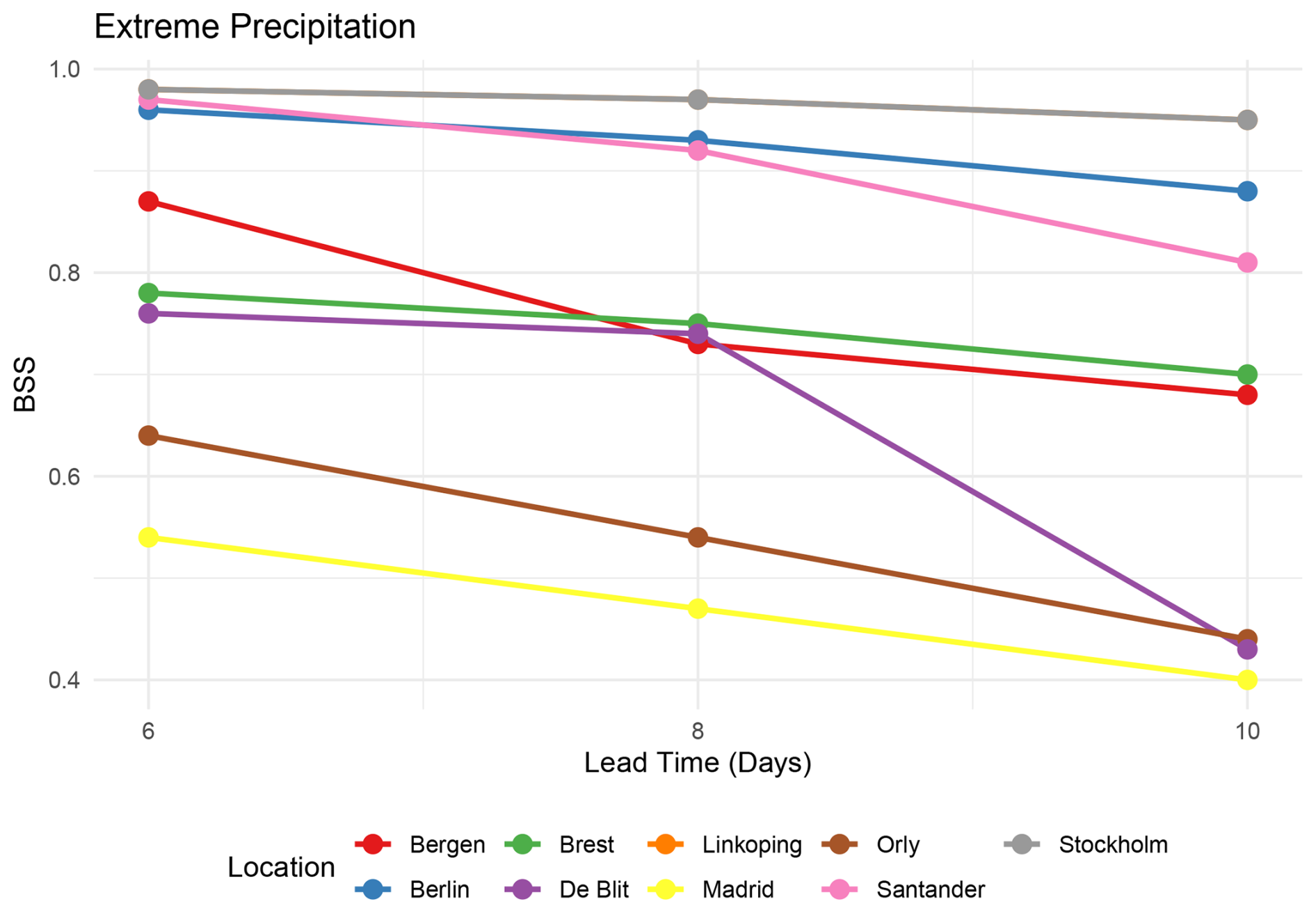
Figure 5 BSS between HC-SWG and the ECMWF forecasts of extreme precipitation for different locations across Europe at different lead times, going from T=6 d to T=10 d, from 2017 to 2021.

To better understand the differences between the two forecasts, we consider the CDFs of the forecasted versus observed extreme precipitation. We use Stockholm and Brest as example stations (Fig. 6). The ECMWF forecast shows very steep CDFs, indicating an under-dispersed ensemble that does not sufficiently capture precipitation variability, leading to an overconfident forecast. In contrast, the HC-SWG forecasts follow the observed CDFs more closely, preserving the distribution's spread and better representing extremes. As the forecast lead time T increases from 6 to 10 d, the ECMWF forecasts remain tightly clustered around a narrow range of precipitation values, suggesting the ensemble struggles to account for increased uncertainty at longer lead times. Meanwhile, the HC-SWG forecasts continue to align well with observations and provide a more reliable probabilistic representation of precipitation. This suggests that incorporating a stochastic approach like HC-SWG can improve ensemble forecast spread and better capture precipitation extremes. The contrast is clear in Stockholm, where the ECMWF ensemble is very concentrated, while the HC-SWG reproduces a much broader distribution that is closer to the observed one. A similar behaviour is found for Brest, showing that this added value is not limited to a single station. At the same time, the HC-SWG CDFs are shifted slightly toward higher precipitation values than the observations in particular for Stockholm at a lead times of 8 and 10 d (Fig. 6b, c), consistent with a tendency to overestimate event magnitude. This helps explain why threshold-based skill scores such as PSS and SEDI remain high: even when the predicted amounts are too large, the forecasts still often correctly identify events as exceeding the chosen quantile. Overall, these results suggest that the main improvement brought by HC-SWG is not only a better identification of extreme-event occurrence, but also a more realistic representation of forecast uncertainty and ensemble spread. For the rest of the stations, we show the comparison between the CDFs of the HC-SWG and the ECMWF forecasts using the using the Kolmogorov-Smirnov test in Table B1 in Appendix B.

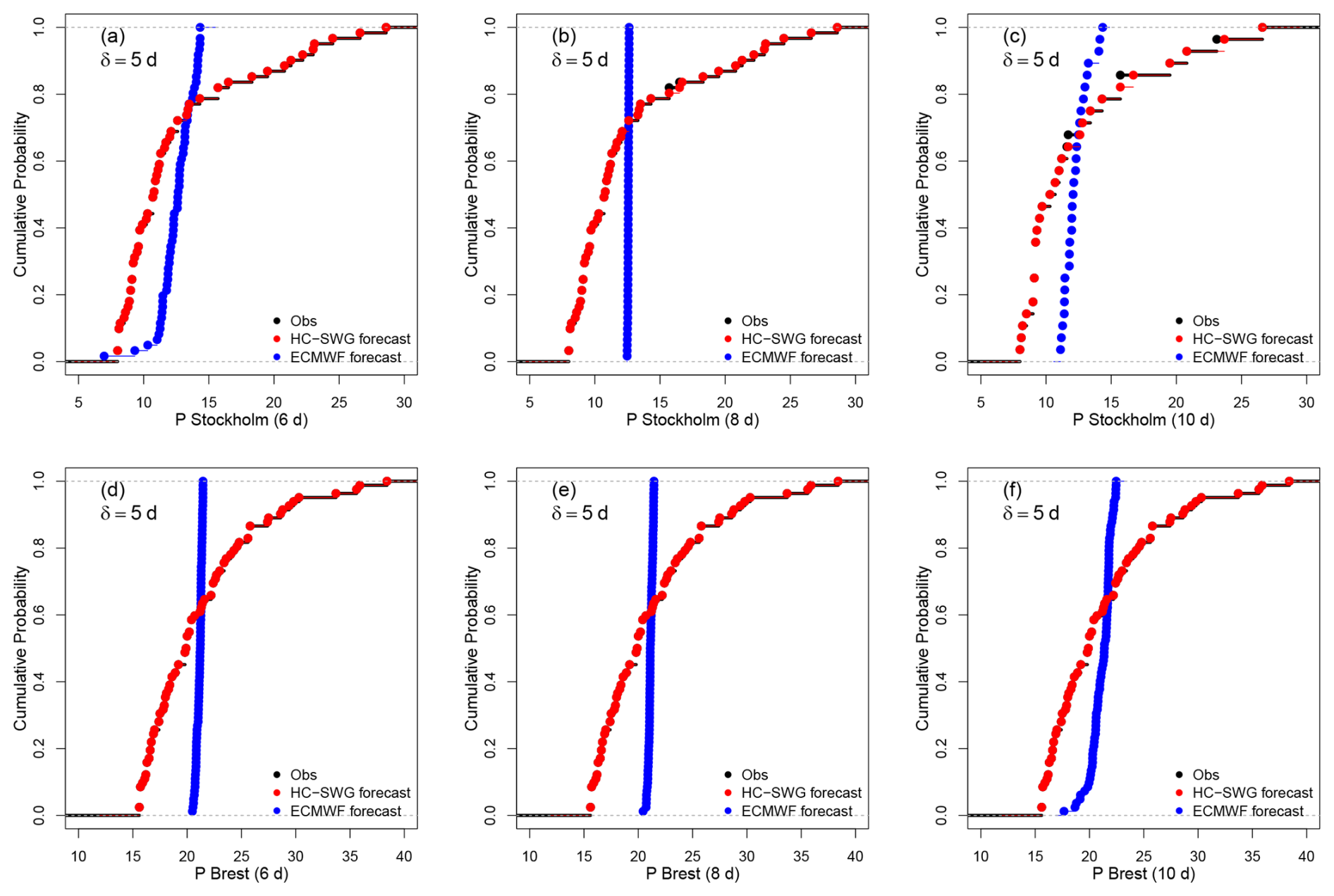
Figure 6 Cumulative Distribution Functions (CDFs) of observed (black) and forecasted (HC-SWG, red; ECMWF, blue) extreme precipitation. We consider Stockholm (a–c) and Brest (d–f) at lead times T=6 (a, d), 8 (b, e) and 10 d (c, f).

4.2 Evaluation of the extreme wind speed forecasts

Unlike HC-SWG, the MA-SWG approach has not been previously tested in the literature. We therefore first test the ability of the MA-SWG to forecast the wind speed on all days, and find that the forecasts provide considerable added value when compared to climatology (Appendix E). We next consider the forecast skill for extreme wind speed only. As for extreme precipitation, we first consider the performance at one example station, here Santander (Fig. 7).

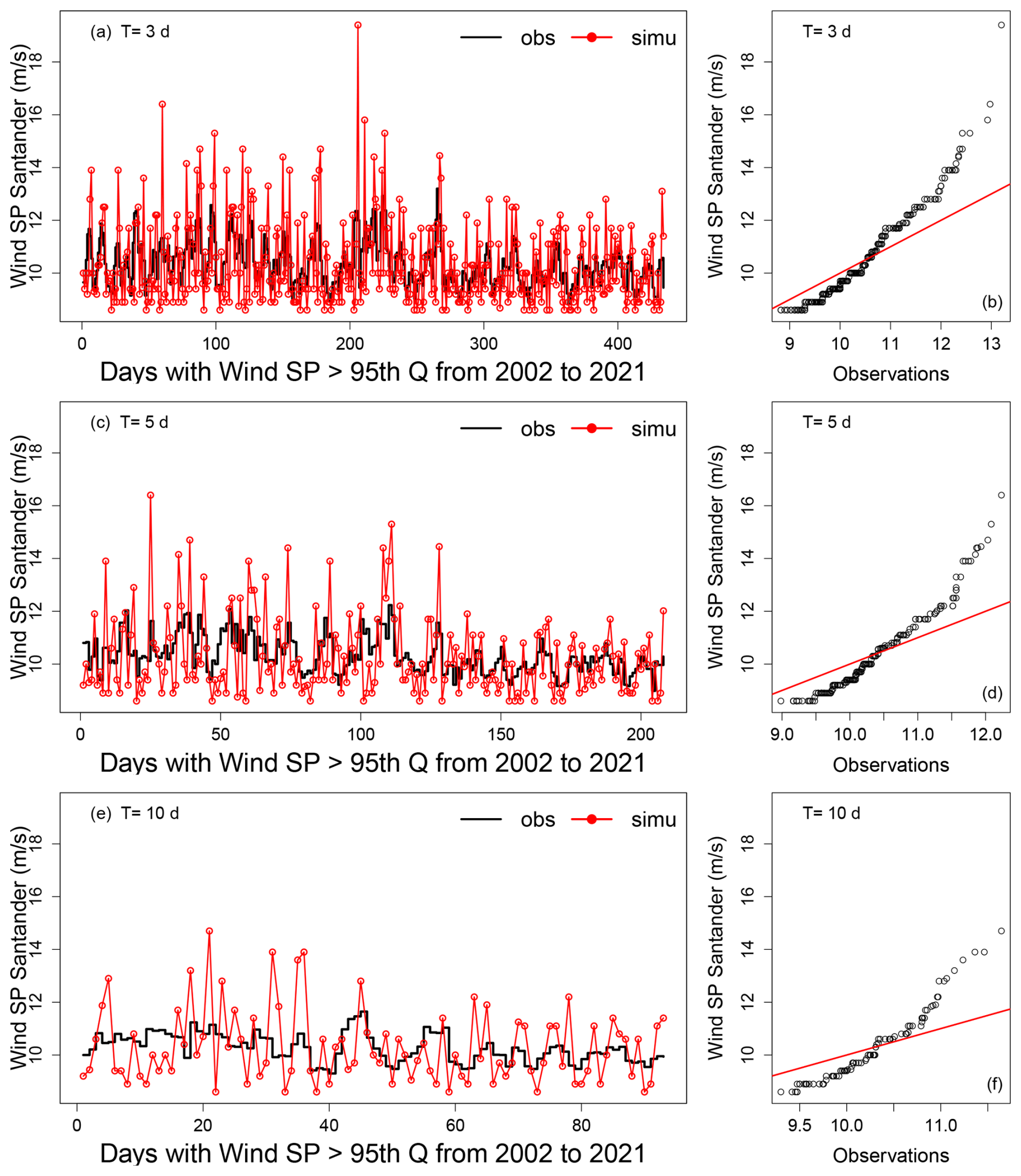
Figure 7 Comparison of observed and forecasted extreme wind speed events using the MA-SWG at lead times T=3, 5 and 10 d for Santander. Panels (a), (c), (e) display time series of observed (black) and forecasted (red, defined as the median of the 100 members) mean wind speeds (m s⁻¹) from 2002 to 2021. Panels (b), (d), (f) present scatter plots comparing observations and forecasts, with the red diagonal lines representing a perfect 1 : 1 relationship.

At all T lead times, the MA-SWG reproduces well the timing of the extreme events. However, it overestimates their magnitude, particularly for the most intense events (Fig. 7b, d, f). This is more pronounced for T=3 d (Fig. 7b) than for T=5 and 10 d (Fig. 7d, f). The MA-SWG thus captures the temporal occurrence of extremes, but it tends to exaggerate their intensity, as we also saw for HC-SWG and extreme precipitation.

We note a similar tendency of MA-SWG to overestimate the most extreme wind speeds also at the other studied stations (Fig. 8). At T=3 d (Fig. 8a), the overestimation is most visible for Santander, Stockholm and Linköping, and similar patterns are visible at T=5 and 10 d (Fig. 8b, c). However, the overall forecast bias appears to decrease on average with forecast lead time T, pointing to a stable tail reliability for longer-range wind forecasts (see Fig. A1 in Appendix A).

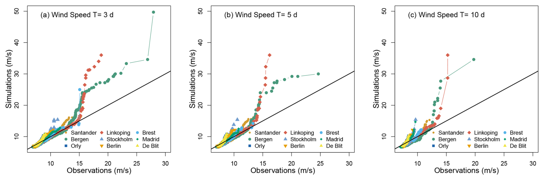
Figure 8 Comparison of observed and forecasted extreme wind speed events using the MA-SWG at lead times T=3 (a), 5 (b) and 10 (c) d for all stations considered here. The panels present scatter plots comparing observed and forecasted wind speed values (m s⁻¹) from 2002 to 2021 on days exceeding the local 95th percentile. The black diagonal lines represent a perfect 1 : 1 relationship.

We next compute PSS and SEDI for the extreme wind forecasts (Fig. 9). The PSS scores (Fig. 9a, c, e) remain consistently high across most stations and lead times, with values close to 1. This indicates that the forecasts are highly skillful in forecasting both extreme and very extreme wind events. Madrid (yellow line in Fig. 9a, c, e) is a clear outlier and displays systematically lower scores than any of the other stations. This may arise from the fact that Madrid displays a higher wind speed variability compared to the other stations.

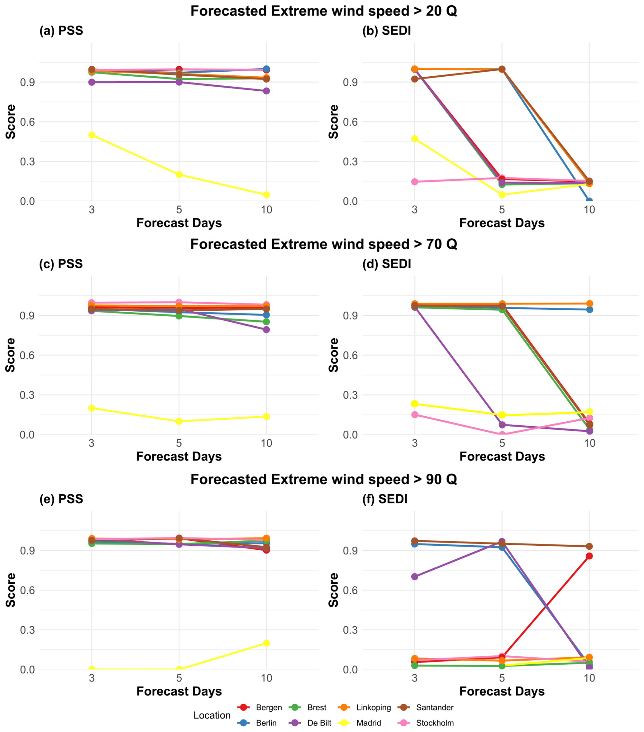
Figure 9 Extreme wind speed forecast skill for MA-SWG evaluated using PSS (a, c, e) and SEDI (b, d, f) at lead times T=3, 5 and 10 d for all stations considered here. We consider separately events above the 20th, 70th and 90th quantiles of the extreme wind speed days (i.e. > 95 Q of the full distribution).

The SEDI scores (Fig. 9b, d, f) vary widely across stations. For stations such as Bergen, they show a steep decline at lead times of 3 and 5 d. This suggests that, while the forecasts remain skilful in detecting extreme wind events (as shown by the high PSS values), their reliability diminishes beyond 5 d for events above the 20th quantile (Fig. 9b), in line with increasing uncertainty in the evolution of synoptic and mesoscale atmospheric features at extended lead times. SEDI also becomes more variable for higher percentiles, indicating that while the MA-SWG correctly forecasts extreme wind speed events in general, its ability to confidently predict the most severe cases is reduced. For events above the 70th and 90th quantiles, SEDI shows a marked increase in inter-station spread with lead time of 3 and 5 d, with some stations maintaining high skill going from 0.92 to 0.95 for Santander and Berlin, and others dropping to very low values. For example, stations such as Bergen and Linköping show a strong degradation at longer lead times, and Madrid remains among the lowest-scoring stations overall. Compared with PSS, SEDI therefore reveals much stronger spatial variability. This indicates that the MA-SWG is generally good at identifying whether a wind-speed threshold will be exceeded, but that its rare-event performance becomes much more station dependent for the strongest events.

Overall, the results indicate that while the forecasts maintain strong discrimination skill (PSS) for extreme wind events, their reliability (SEDI) varies across stations and decreases for the most extreme cases.

We next compare the MA-SWG and ECMWF forecasts for 10 m wind speed extremes at different lead times using the BSS (Fig. 10). The BSS for all the studied stations is positive, which indicates that MA-SWG outperforms ECMWF. The magnitude of the improvement varies across stations, and generally decreases with increasing lead time. At T=3 d, values range between 0.62 and 0.97, while they decrease to between 0.41 and 0.91 at T=10 d (Fig. 10). Thus, the added value of MA-SWG over ECMWF is robust across all stations, although its magnitude is clearly location dependent and tends to weaken with lead time.

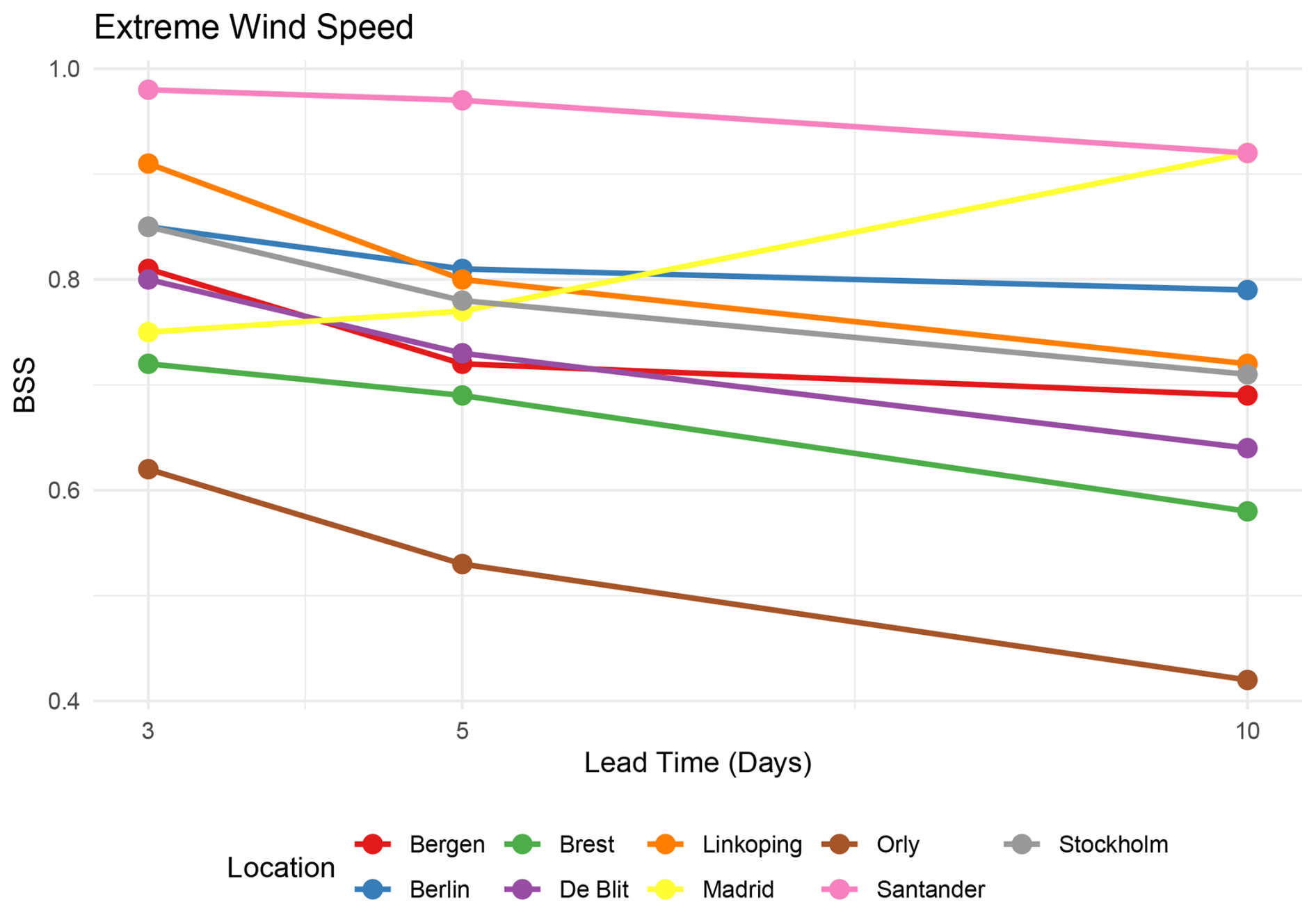
Figure 10 BSS between the MA-SWG forecast and the ECMWF forecasts of extreme wind speed for different locations across Europe at different lead times, going from T=3 d to T=10 d, from 2017 to 2021.

As for the HC-SWG extreme precipitation forecasts, we compare the CDFs of the MA-SWG and ECMWF wind speed forecasts to the CDFs of the observations, showing Stockholm and Brest as examples (Fig. 11). For both stations, the CDFs of observations and the MA-SWG forecasts show a close agreement. The ECMWF forecasts instead underestimate the most extreme wind speed values and overestimate the lowest values, the latter in particular for Stockholm at 3 and 5 d (Fig. 11a, b). For Brest, the CDFs of the ECMWF forecasts are generally closer to observations, but they keep underestimating the most extreme values. The contrast is particularly clear in Stockholm, where the ECMWF distribution is shifted toward weaker wind extremes, while the MA-SWG better reproduces the upper tail of the observed distribution. In Brest, the difference between the two forecasts is smaller, except for lead time 10 d, but MA-SWG still provides a better representation of the strongest events, especially at longer lead times. As for the extreme precipitation, for the other stations we compare the CDFs of extreme wind forecasts from MA-SWG and ECMWF using the Kolmogorov-Smirnov test and results are represented in Table B1 in Appendix B.

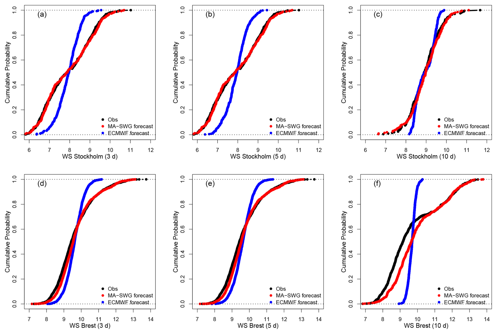
Figure 11 Cumulative Distribution Functions (CDFs) of observed (black) and forecasted (MA-SWG, red; ECMWF, blue) extreme wind speed. We consider Stockholm (a–c) and Brest (d–f) at lead times T=3 (a, d), 5 (b, e) and 10 d (c, f).

4.3 Assessment of Compound forecasts

We now evaluate the capacity of the SWG to forecast extreme precipitation and extreme wind speed events, which occur simultaneously or sequentially, following the procedure described in Sect. 3.1.

We find that, for a forecast of T=10 d, the SWG is able to reproduce very closely the observed frequency of occurrence of simultaneous extreme precipitation and wind speed, as shown in Table 1. In particular, the SWG correctly identified three of the four stations that display no such events in observations, and reproduces a very low frequency of occurrence for the fourth station.

Table 1 Simultaneous occurrences of extreme precipitation and extreme wind speed events from 2002 to 2021 in observations and SWG forecasts. The percentages are relative to the total number of forecasted or observed extreme precipitation and wind speed events. The total number of extremes at each location in the SWG forecasts is indicated in parentheses.

We performed a similar analysis for sequential events. Figure 12 shows the number of extreme precipitation events followed by extreme wind, and extreme wind events followed by extreme precipitation, using time windows ranging from 1 to 5 d. The number of sequential events by definition increases with longer time windows, as these allow more chances for one type of event to follow the other. The results reveal strong spatial variability in the number of both types of events. For instance, locations like Brest, Bergen, De Bilt, and Santander (Fig. 12a, c, d, i) show a higher number of extreme wind events followed by extreme precipitation events, consistent with Atlantic-driven storm systems that often bring strong winds before heavy rain. In contrast, Berlin, Linköping, Madrid and Orly (Fig. 12b, e, f, g) show comparable or higher numbers of extreme precipitation events followed by extreme wind speed than extreme wind speed events followed by extreme precipitation. Finally, Stockholm (Fig. 12h) shows very few sequential events.

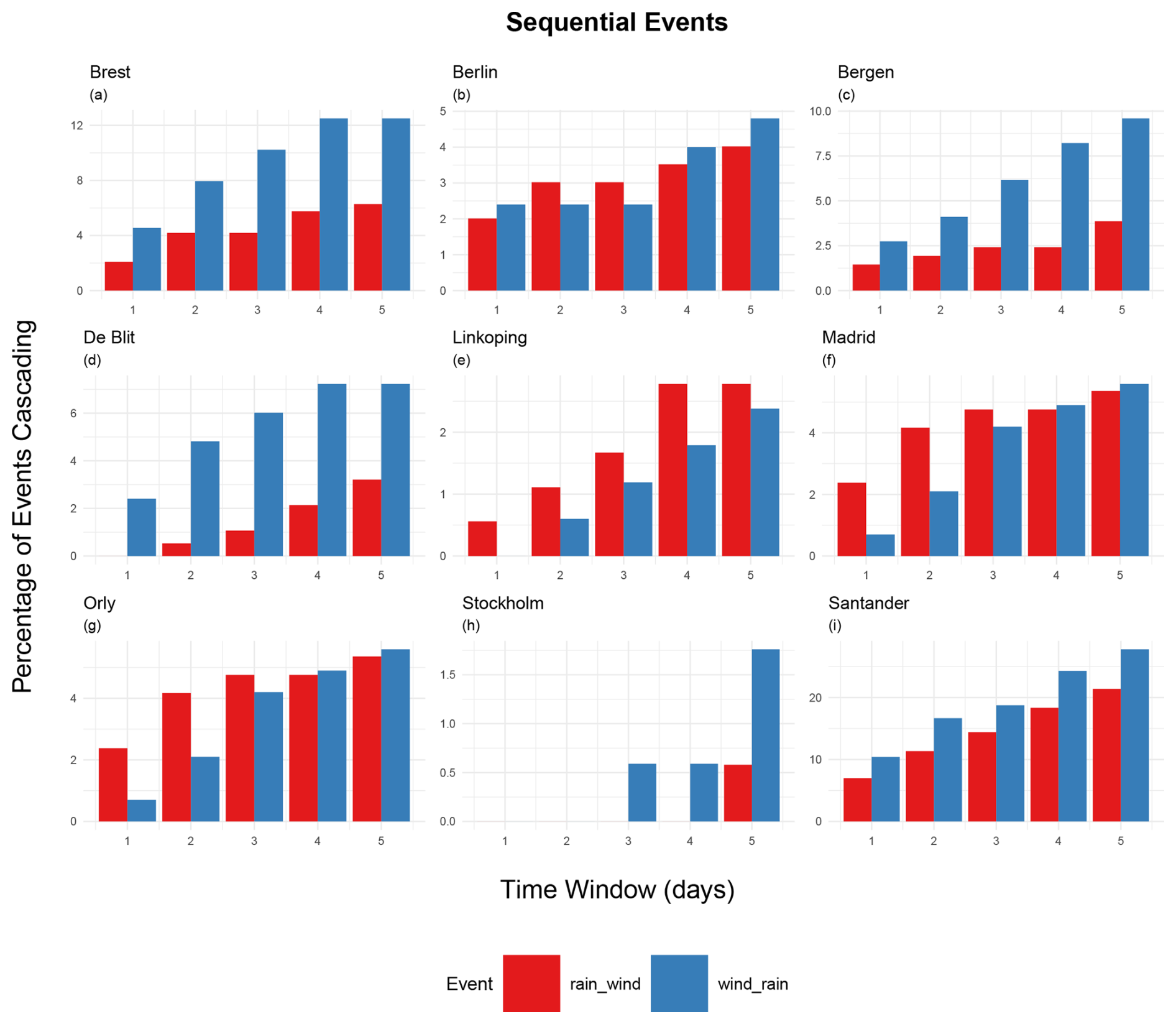
Figure 12 Percentage of extreme precipitation or wind events which are followed by the other extreme, as forecasted by the SWG at lead time T=10 d. Red represents events where extreme precipitation is followed by extreme wind, and blue represents events where extreme wind is followed by extreme precipitation. We consider time windows (lags between the two extreme weather events) from 1 to 5 d. The y-ranges differ between panels.

We next compared the sequential extremes in SWG forecasts to those in observations (Fig. 13). Compared to observations, the SWGs capture the general frequency of occurrence of sequential events reasonably well, especially for Stockholm, Orly, Madrid and Bergen (Fig. 13c and f). Overestimations are notable in locations like Santander and Brest for both types of sequential events, particularly for longer time windows (3–5 d). De Bilt shows a systematic overestimation of extreme windspeed events followed by extreme precipitation (Fig. 13f). There is a single instance of SWG forecasts underestimating the frequency of occurrence of sequential extremes, namely De Bilt for rain extremes followed by wind speed extremes for a time window of two days (Fig. 13c).

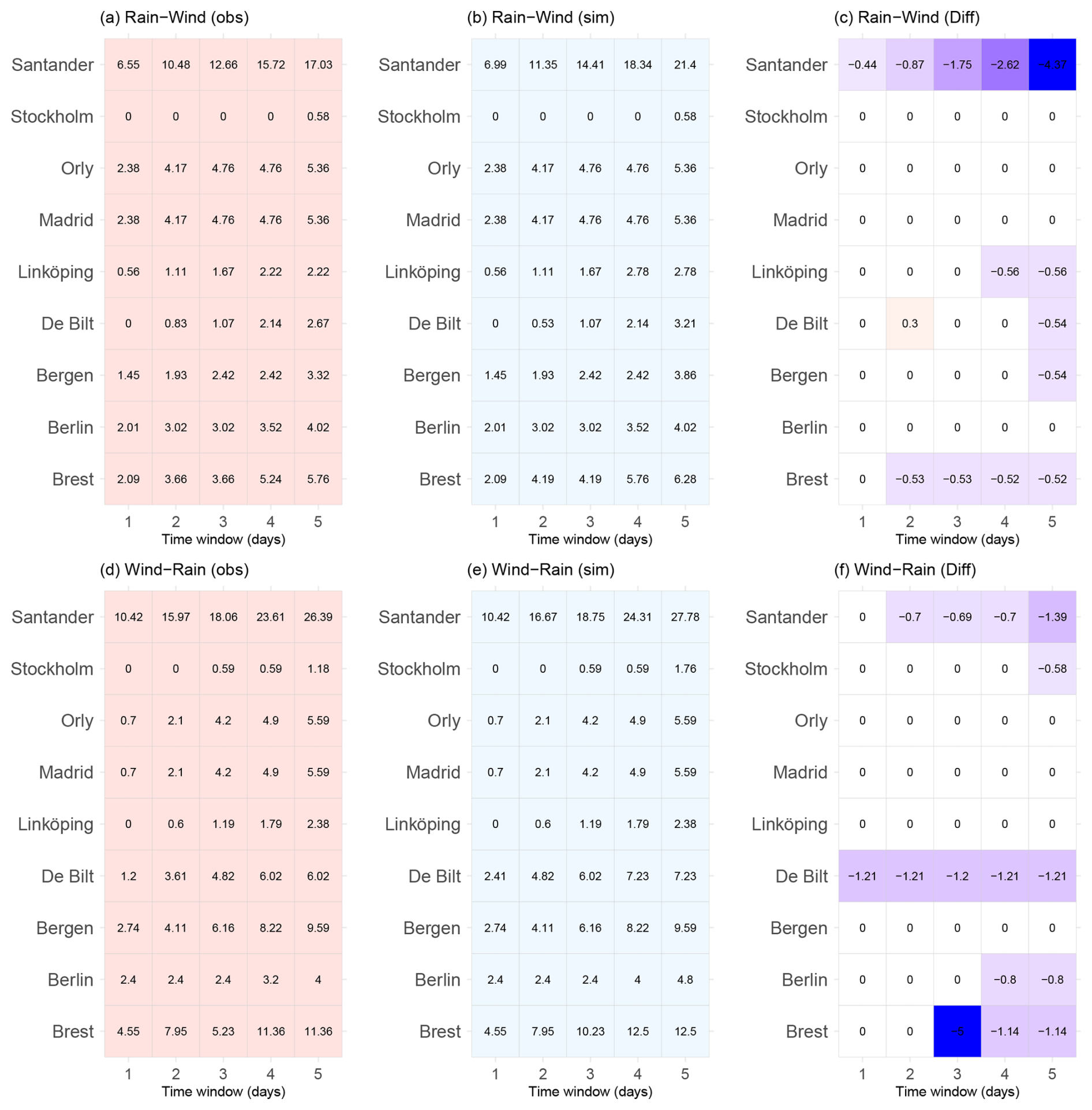
Figure 13 Comparison of the percentage of Rain → Wind and Wind → Rain sequential extreme events as identified in observations (a, d) and simulated using the SWGs at lead time T=10 d (b, e) across the studied locations for varying time windows (1 to 5 d). Panels (c) and (f) present the differences between observed and simulated percentages (Obs – Sim). Positive values indicate an underestimation by the SWG forecasts, while negative values indicate an overestimation.

The above results suggest that the SWG forecasts, while displaying some biases, nonetheless capture key regional features of compound wind-precipitation extremes. They thus offer a promising approach for simulating and predicting compound hazards.

5 Conclusions

This study presents and evaluates two ensemble forecasting approaches based on stochastic weather generators: the HC-SWG and the MA-SWG. We used the first to forecast extreme precipitation, and the second to forecast extreme wind speed across different locations in Europe. Both approaches integrate analogs of the large-scale atmospheric circulation with a stochastic weather generator to produce ensemble forecasts at medium-range lead times of up to 10 d.

The HC-SWG uses analogs from the ECMWF Z500 ensemble reforecasts. The MA-SWG uses multivariate analogs defined from the ERA5 reanalysis of Z500 and SLP. The two approaches thus differ fundamentally in their input sources. The HC-SWG indirectly benefits from flow-dependent information and information on ensemble spread as provided by the reforecasts. In contrast, the MA-SWG relies on the long historical record of the ERA5 reanalysis and on multi-variable patterns to capture large-scale circulation features.

Both SWG approaches show strong skill in forecasting extreme events up to 10 d ahead, outperforming ECMWF forecasts across different evaluation metrics and lead times. The HC-SWG displays high Peirce Skill Score (PSS) and Symmetric Extremal Dependence Index (SEDI) values across locations. MA-SWG shows greater spatial variability yet generally positive SEDI values. The SWG forecasts also display a strong performance in reproducing the observed frequency of simultaneous and sequential extreme precipitation and wind speed extremes.

Notwithstanding their strong performance, the SWG forecasts still show limitations. Indeed, the forecast skill can be location dependent, likely due to local processes that are not well captured by the large-scale circulation analogs. Both SWG methods also overestimate the intensity of the most extreme events. For HC-SWG, this could be related to the relatively short timespan covered by the ECMWF reforecasts, limiting the availability of good circulation analogs for these rare cases. Future work could explore calibration strategies to reduce such biases and extend the SWG approach to other compound event types or geographical regions.

To conclude, we find that SWG forecasts outperform a set of recent numerical forecasts for extreme wind and precipitation in Europe, and correctly reproduce the frequency of compound wind and precipitation extremes. This highlights the potential of SWG forecasts for use in early-warning applications of compound hazards, which pose a key challenge for current forecasting tools.

Appendix A: Forecast Bias

We evaluated the SWG forecast bias for extreme wind speed (Fig. A1a) and extreme precipitation (Fig. A1b) across the studied European locations at different lead times. The forecast bias was defined as the mean difference between the simulated (sim) and observed (obs) extreme precipitation or extreme wind speed at each lead time T and for each station as follows:

$$\begin{array}{}\text{(A1)}& \mathrm{Bias}={\displaystyle \frac{\stackrel{\mathrm{‾}}{\mathrm{sim}}-\stackrel{\mathrm{‾}}{\mathrm{obs}}}{\stackrel{\mathrm{‾}}{\mathrm{obs}}}}\end{array}$$

For extreme wind speed, MA-SWG forecasts show a positive bias across most locations and lead times, indicating a systematic overestimation (Fig. A1a). This overestimation is particularly notable for Santander, while it is moderate for all the other stations. In contrast, the bias for extreme precipitation is more variable, both spatially and with lead time (Fig. A1b). Several locations, including Brest, Berlin, and Bergen, show a strongly negative bias at longer lead times (notably at T=10 d), suggesting underestimation of high precipitation amounts. Others, like Madrid, De Bilt and Stockholm, maintain near-zero or slightly positive biases. The MA-SWG thus appears to overpredict wind extremes, while the HC-SWG results are more variable, yet the forecasts tend to underpredict precipitation extremes as the forecast lead time increases.

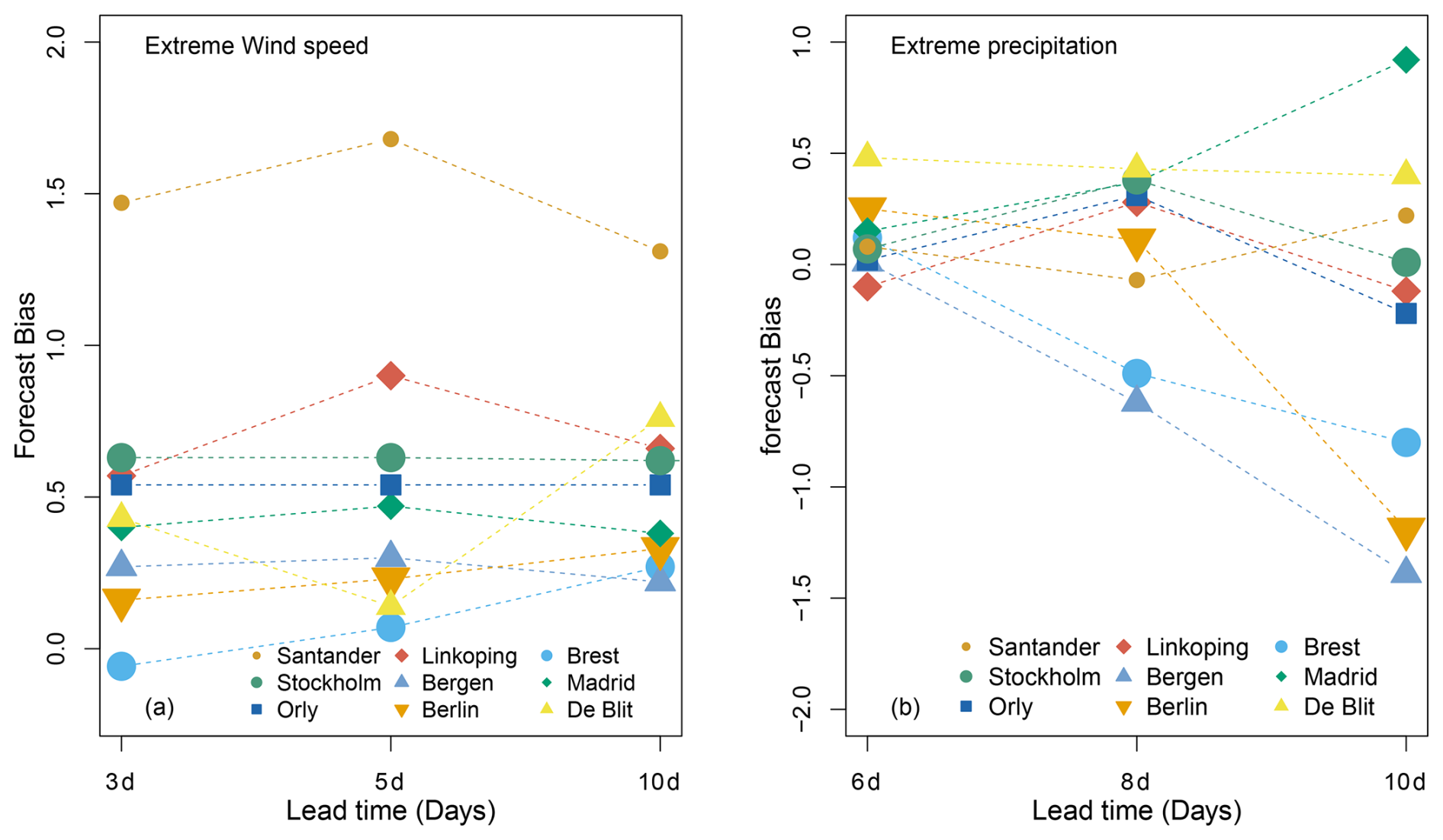
Figure A1 Bias of the MA-SWG and HC-SWG forecasts for extreme wind speed (a) and extreme precipitation (b), computed against observations for different lead times T from 3 to 10 d for all stations considered here.

Appendix B: Comparison of the SWGs forecasts to the ECMWF forecast

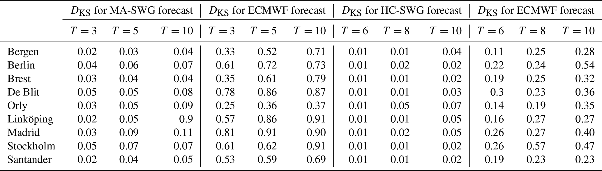
We compare the performance of the SWGs forecast to the ECMWF forecast for all stations using D values from the Kolmogorov-Smirnov test (Table B1). D quantifies the maximum distance between two CDFs, with higher values indicating larger distances. At all lead times and for all stations, MA-SWG and HC-SWG display lower D than ECMWF forecast (Table B1), indicating very similar distributions between SWGs forecasts and observed extremes.

Table B1 Comparison of the CDFs of extreme wind speed forecasts from MA-SWG and extreme precipitation forecasts from HC-SWG, to the respective ones from the ECMWF forecast for different lead times T days with observations, using Kolmogorov-Smirnov D_KS values. The D values are determined between each forecast and observations.

Appendix C: Additional forecast evaluation metrics

To evaluate wind speed forecasts in Appendix E, we use the Continuous Ranked Probability Skill Score (CRPSS) and temporal correlation. This mirrors the evaluation performed in Krouma et al. (2024) for precipitation forecasts. We also use the area under the Receiver Operating Characteristic (ROC) curve to evaluate the forecasts of extreme wind speed, again in line with the evaluation conducted in Krouma et al. (2024) for extreme precipitation.

To compute CRPSS we first compute the Continuous Ranked Probability Score (CRPS), which serves as a quadratic metric to measure discrepancies between the forecasted CDF and the empirical CDF derived from observed data (Wilks, 2011; Zamo and Naveau, 2018). The CRPS is defined as:

$$\begin{array}{}\text{(C1)}& \mathrm{CRPS}(P,x_a)=\underset{-\mathrm{\infty }}{\overset{+\mathrm{\infty }}{\int }}\left(P\right(x)-\mathcal{H}(x-x_a){)}^{\mathrm{2}}\mathrm{d}x,\end{array}$$

where x_a represents the observed values of x within the period [t₀ , t₀+T], P is the cumulative distribution function of x from the ensemble forecast, and ℋ denotes the Heaviside function, defined as ℋ(y)=1 if y≥0 and ℋ(y)=0 otherwise. A perfect forecast yields a CRPS value of 0. As the CRPS depends on the variable's unit, it is beneficial to normalize it relative to the CRPS of a reference forecast, such as persistence or climatology. The Continuous Ranked Probability Skill Score (CRPSS) expresses the percentage improvement over such a reference forecast (Hersbach, 2000), given by:

$$\begin{array}{}\text{(C2)}& \mathrm{CRPSS}=\mathrm{1}-{\displaystyle \frac{\stackrel{\mathrm{‾}}{\mathrm{CRPS}}}{\stackrel{\mathrm{‾}}{{\mathrm{CRPS}}_{\mathrm{ref}}}}},\end{array}$$

Here, $\stackrel{\mathrm{‾}}{\mathrm{CRPS}}$ is the mean CRPS of the SWG forecast and $\stackrel{\mathrm{‾}}{{\mathrm{CRPS}}_{\mathrm{ref}}}$ is the mean CRPS of climatology.

The Area Under the ROC Curve (AUC) quantifies the discrimination skill of a forecast, measuring how well it differentiates between event and non-event occurrences. Higher AUC indicates a superior ability to distinguish between events and non-events (Fawcett, 2006; Toth et al., 2003), with values near 0.5 representing no skill (random chance). We evaluated the AUC for two wind speed thresholds, respectively the 70th and 90th quantiles, considering events below those thresholds as non-events.

The Brier score (BS) evaluates the accuracy of probabilistic forecasts by computing the mean squared difference between the forecast probabilities of a given event and the observed binary outcomes (Stephenson et al., 2008b; Wilks, 2011). It is given by:

$$\begin{array}{}\text{(C3)}& \mathrm{BS}={\displaystyle \frac{\mathrm{1}}{N}}\sum _{i=\mathrm{1}}^N(f_i-o_i{)}^{\mathrm{2}},\end{array}$$

where N is the number of forecasts, f_i is the predicted probability of the event occurring, and o_i is the observed outcome (1 if the event occurred, 0 otherwise). A lower Brier Score indicates better forecast accuracy. We compute the Brier skill Score (BSS) against climatology to evaluate the sensitivity of HC-SWG forecast skill to different reforecasts δ in Appendix D.

The use of these different skill scores provides a comprehensive evaluation of how HC-SWG and MA-SWG predict extreme precipitation events, wind speed, and extreme wind speed events.

Appendix D: Forecast evaluation as a function of reforecast lead time for extreme precipitation with HC-SWG

To assess the sensitivity of the extreme precipitation forecast to the different δ lead times of Z500 analogs used as inputs to the HC-SWG, we used the Brier Skill Score (BSS) that we compute against the climatology. Figure D1 illustrates the sensitivity of HC-SWG forecast skill for extreme precipitation, as measured by the BSS, to both the precipitation forecast lead time (T, from 2 to 10 d) and the hindcast lead time of Z500 (δ, from 1 to 5 d), which is used as input to the SWG.

The forecasts show better probabilistic skill (higher BSS values against climatology) at lead times T closer to δ values. As T increases for the same δ, the BSS decreases, implying that forecasts initialized with older Z500 hindcasts lose accuracy, particularly at longer precipitation T lead times. These results emphasize that both lead time and the choice of atmospheric conditions used for determining the analogs play a crucial role for the forecast skill of extreme precipitation, with large-scale atmospheric states close to the forecast initialisation date providing better predictive information compared to more distant ones.

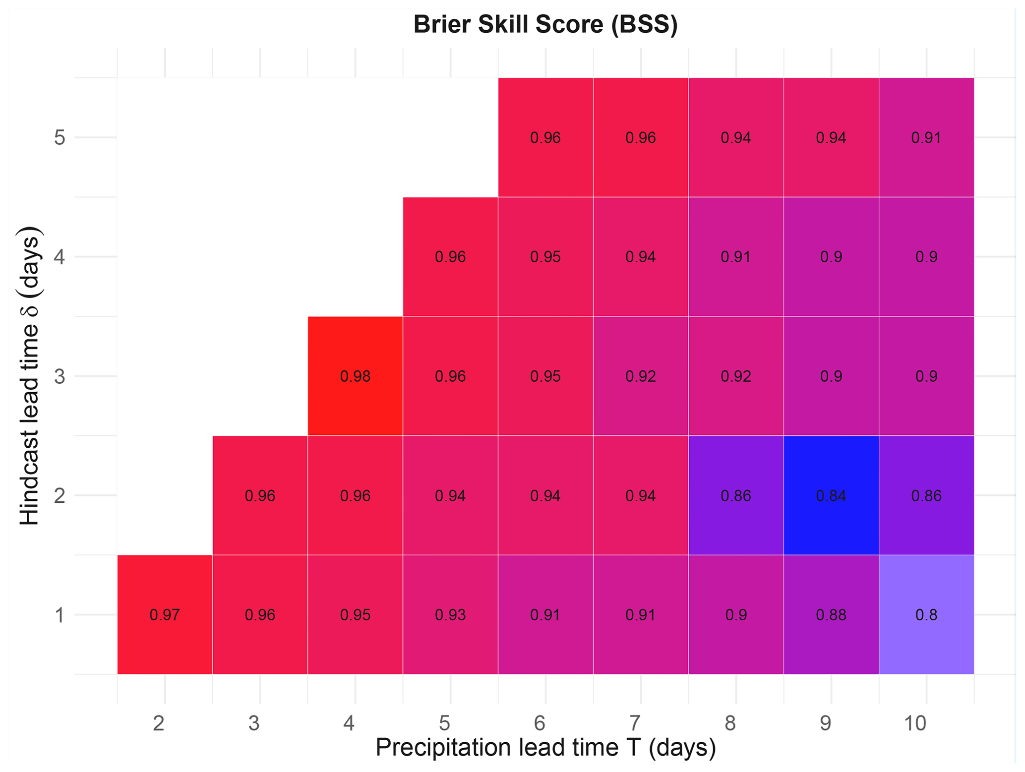
Figure D1 Brier Skill Score (BSS) of the HC-SWG forecast performance for extreme precipitation at different forecast lead times T and for different δ lead times of the ECMWF Z500 ensemble reforecasts.

Appendix E: Forecast evaluation for wind speed and wind speed extremes with MA-SWG

We start by evaluating the forecast skill of MA-SWG for wind at 10 m, as the SWG was not tested in any previous studies to forecast the wind in Europe.

Figure E1 presents the CRPSS for wind forecasts at different lead times (1, 3, 5, 10, and 20 d) relative to a climatological reference for summer (JJA, Fig. E1a) and winter (DJF, Fig. E1b). In both seasons, forecast skill decreases with increasing lead time, with the sharpest decline occurring between 1 and 5 d lead times, followed by a more gradual reduction at longer lead times.

CRPSS values are always positive, indicating that the MA-SWG forecasts systematically provide an added value relative to climatology. Overall, CRPSS values are higher in winter than in summer, whereas JJA forecasts show high variance across locations with CRPSS values varying between 0.93 and 0.58 at T=1 d. The seasonal difference in forecast skill may be attributed to the fact that atmospheric conditions are more predictable in winter, and the correlation between atmospheric circulation and surface variables is stronger in that season (Laurila et al., 2021). This is particularly relevant given that we are using Z500 and SLP as predictors. Some locations, such as Bergen, Linköping and Santander, consistently show higher CRPSS values than the other stations in both seasons. Others, such as Stockholm and Berlin, systematically exhibit amongst the lowest skills. These location-specific variations may be due to regional climate differences and local topography. Overall, wind forecasts perform better in winter, with skill declining with increasing lead time T and a pronounced location dependence in both seasons.

Figure E2 provides information corresponding to Fig. E1 but for the correlation between wind forecasts and observations. In both seasons, at short lead times (1 d), most locations show high correlation values (∼ 0.6–0.8), indicating strong predictive skill. The correlation decreases with increasing lead time, with a sharp drop between 1 and 5 d lead times. Winter (DJF) forecasts generally exhibit higher correlations than summer (JJA) forecasts, supporting previous results in Fig. E1. Indeed, summer forecasts diplay relatively low correlations already at 3 d lead times, likely due to increased atmospheric instability and more localised high-wind events compared to winter. Bergen and Santander tend to exhibit amongst the highest correlations in JJA, whereas Orly and Berlin emerge as displaying amongst the lowest correlations in DJF. Overall, winter wind forecasts are more consistent with observations than summer forecasts, with location-dependent variations becoming more pronounced as lead time increases.

Figure E3 presents AUC values for wind speed forecasts exceeding 70 Q (Fig. E3a) and 90 Q (Fig. E3b) at the same lead times and stations as in the previous figures. In both cases, forecast skill decreases with increasing lead time, particularly for the 90 Q threshold. AUC values are generally higher for the 70 Q threshold than for the 90 Q threshold, suggesting better predictability for more moderate wind events. Nonetheless, the spread between locations is higher for the lower wind threshold. Some locations, such as Berlin, Linköping and Orly, maintain relatively high skill levels over time, whereas others such as Bergen and Madrid show a more rapid degradation in AUC, particularly beyond 5–10 d. For the 90 Q threshold, at longer lead times (10–20 d), several locations have AUC values close to or below 0.5, suggesting that forecasts provide little added value over random chance. Overall, wind forecasts are more skillful for lower wind speed thresholds (wind speed >70 Q) and shorter lead times, while forecasts for higher wind speed extremes (wind speed >90 Q) come with greater uncertainty.

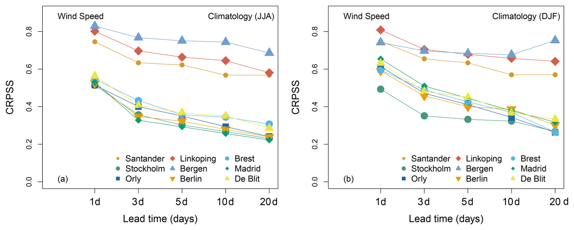
Figure E1 CRPSS with respect to climatology for the MA-SWG forecasts of wind speed. Forecasts for (a) JJA and (b) DJF for lead times of T=1, 3, 5, 10 and 20 d, for all stations considered here.

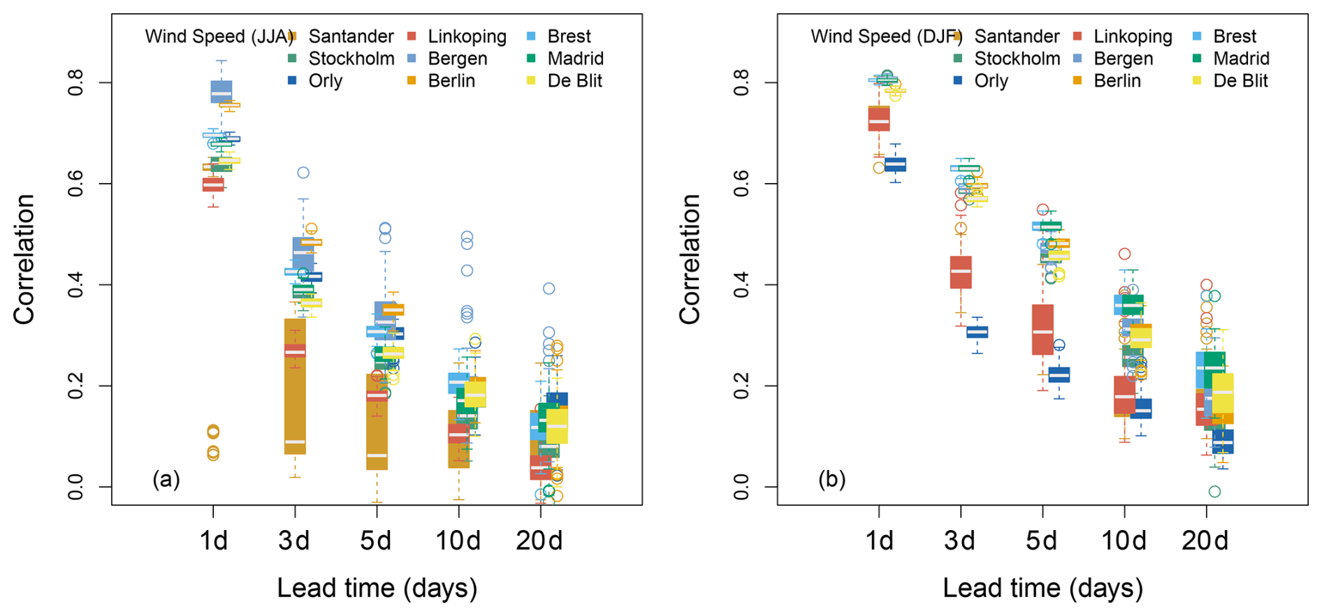
Figure E2 Rank Correlation between the MA-SWG forecasts of wind speed and observations. Forecasts for (a) JJA and (b) DJF for lead times of T= 1, 3, 5, 10 and 20 d, for all stations considered here.

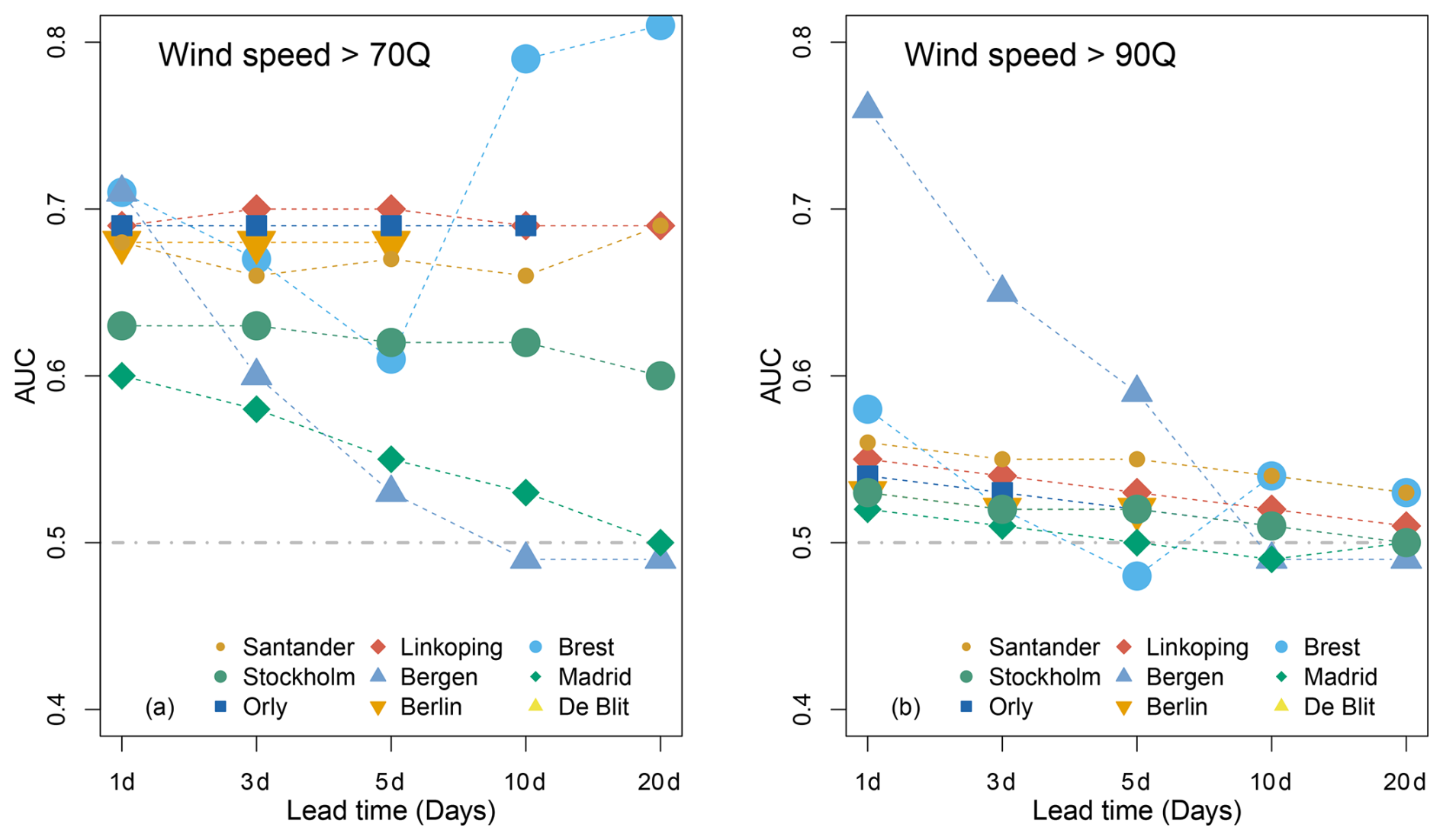
Figure E3 AUC for the MA-SWG wind speed forecasts for (a) wind speed events exceeding the 70 Q threshold, and (b) wind speed events exceeding the 90 Q threshold. The dashed grey lines represent AUC=0.5.