From single storms to large-scale waves: a multi-year kilometer-scale global simulation

Global kilometer-scale (km-scale) weather and climate models offer new opportunities to unify numerical weather prediction (NWP) and climate modeling by explicitly simulating convection and mesoscale circulations globally within a single modeling framework. We present results from the first multi-year (April 2020–March 2024) global atmosphere-land simulation using the GPU-refactored ICON model at a 2.5 km horizontal grid spacing and 120 vertical levels. The simulation uses NWP physics and observed sea-surface temperatures. We assess its performance against satellite, reanalysis, and in-situ observations using standard statistics and the MOAAP feature-tracking framework to evaluate a wide spectrum of atmospheric phenomena. ICON reproduces global temperature and precipitation patterns, including a realistic single Intertropical Convergence Zone and physically consistent diurnal precipitation cycles. However, ICON exhibits continental summertime warm and dry biases, linked to an overestimation of incoming solar radiation and excessive surface sensible heat fluxes. The model realistically captures the intensity and frequency of hourly precipitation and near-surface winds, as well as the structure and occurrence of tropical cyclones. Mesoscale convective systems (MCSs) exhibit realistic spatial initiation patterns, but their frequency is underestimated over oceans and overestimated over tropical land. Long-lived MCSs are too infrequent and small, while increased rainfall from shallow and mid-level clouds may reflect overactive warm-cloud microphysics or observational deficiencies. These biases might stem in part from a misrepresentation of thermodynamic-convection coupling. Our results demonstrate the feasibility and scientific value of multi-year global km-scale simulations for exploring the weather–climate system and local-scale extreme events, while identifying key directions for future model development.

1 Introduction

The consequences of anthropogenic climate change are increasingly visible through record-breaking extreme events and their associated impacts (e.g., Donat et al., 2016; IPCC, 2023; Seneviratne et al., 2023; Perkins-Kirkpatrick and Lewis, 2020). Reliable, local-scale climate information to support adaptation and mitigation efforts is urgently needed, as many extremes and their impacts occur at spatial scales that are poorly represented in state-of-the-art global climate models (Giorgi and Gutowski, 2015; IPCC, 2023). Kilometer-scale (km-scale) weather and climate models, with horizontal grid spacings of a few kilometers, have emerged as promising tools to bridge this gap by explicitly resolving deep convection, orographic flows, and other mesoscale phenomena (Prein et al., 2015; Kendon et al., 2017; Lucas-Picher et al., 2021). However, the computational cost of km-scale modeling has historically restricted its use to limited-area domains over relatively small regions. Recent advances in model development, numerical efficiency, and high-performance computing now enable month- to multi-year-long km-scale simulations to be conducted globally (Stevens et al., 2019; Schär et al., 2020; World Climate Research Programme, 2022), opening unprecedented opportunities to study mesoscale processes and their interactions with synoptic- and planetary-scale circulations within a physically consistent framework.

Regional km-scale climate modeling has rapidly evolved over the past decade and has now reached a mature stage of scientific and technical development (Prein et al., 2015; Ban et al., 2014; Kendon et al., 2021; Marsham et al., 2013). A central research focus has been to identify the added value of km-scale simulations compared to coarser, convection-parameterized models. Numerous studies have demonstrated that the intermittency, intensity, frequency, and phase of precipitation are substantially improved when deep convection is explicitly resolved (e.g., Holloway et al., 2012; Prein et al., 2013; Ban et al., 2014; Kendon et al., 2017). In particular, sub-daily precipitation extremes are much better captured (e.g., Ban et al., 2014; Prein et al., 2015, 2017; Ban et al., 2021; Pichelli et al., 2021) and the diurnal cycle of convective precipitation is more realistically represented (e.g., Sato et al., 2009; Marsham et al., 2013; Ban et al., 2014; Prein et al., 2013). Furthermore, the spatial organization of convection, including mesoscale convective systems and tropical cyclones, is substantially improved in km-scale models (e.g., Miura et al., 2007a; Gentry and Lackmann, 2010; Clark et al., 2016; Prein et al., 2020, 2021, 2022; Gutmann et al., 2018). Consistent with the explicit treatment of deep convection, km-scale simulations also produce convective wind gusts and straight-line winds that are absent in models with parameterized convection (Prein, 2023; Brown et al., 2024). Improved representation of topography enhances the simulation of orographic precipitation, mountain snow accumulation, and valley wind systems (Liu et al., 2017; Ikeda et al., 2021; Schmidli et al., 2018). Additionally, km-scale grids allow for a more faithful representation of land–atmosphere coupling (Hohenegger et al., 2009; Lee and Hohenegger, 2024; Segura et al., 2022), and lateral groundwater fluxes can be represented explicitly, which can feed back on soil moisture and precipitation characteristics (Schlemmer et al., 2018; Barlage et al., 2021). At km-scale resolution, urban areas can be better represented, enabling more realistic simulations of urban heat islands and their influence on local convection and precipitation (Argüeso et al., 2016; Langendijk et al., 2021). However, dedicated land surface model development efforts are needed to include processes that are typically missing (e.g., shallow groundwater flow, urban parameterizations).

While many of the mesoscale phenomena examined here have already been studied with regional convection-permitting models, the added value of the present study is that it evaluates them within a single, consistent, multi-year, global km-scale framework, enabling direct comparisons across regions and assessments of their links to larger-scale circulation features.

The field of global km-scale modeling was pioneered by the Japanese community (Tomita et al., 2005; Miura et al., 2007b; Satoh et al., 2008) through the development of the Non-hydrostatic ICosahedral Atmospheric Model (NICAM). Over the last two decades, almost every major model-development center has invested in developing next-generation, non-hydrostatic global modeling capabilities. At the same time, advances in computer technology made it feasible to run global km-scale simulations for more than just a few days. The DYAMOND (DYnamics of the Atmospheric general circulation Modeled On Non-hydrostatic Domains) intercomparison experiments leveraged these developments and initiated the first global, multi-model, km-scale coordinated intercomparison of simulations of the atmosphere at grid spacings of 3–5 km (Stevens et al., 2019; Satoh et al., 2019; Takasuka et al., 2024b). These experiments revealed substantial inter-model differences in the ability to simulate mesoscale convective systems (MCSs) (Feng et al., 2025) and tropical cyclones (Judt et al., 2021). Some modeling systems demonstrated notable progress following dedicated model development efforts. For instance, the U.S. Department of Energy's SCREAM (Simple Cloud-Resolving E3SM Atmosphere Model) initially underestimated convective organization during the first DYAMOND phase but demonstrated marked improvements in MCS and tropical-cyclone structure in DYAMOND-Winter after major revisions to microphysics and numerics (Taylor et al., 2023; Donahue et al., 2024; Feng et al., 2025). Beyond convective systems, global km-scale simulations exhibit more realistic representations of equatorial waves and tropical variability compared to coarser-resolution models (Miura et al., 2007a; Nasuno et al., 2008; Holloway et al., 2012; Weber and Mass, 2019; Judt and Rios-Berrios, 2021). Ongoing developments extend these atmospheric configurations toward multidecadal coupled ocean-atmosphere-land models that include interactive ocean, sea ice, and biogeochemical components (Hohenegger et al., 2023; Segura et al., 2025b; Rackow et al., 2025) as well as the carbon cycle and aerosol emissions (Klocke et al., 2025).

Here, we present an overview of the performance of a global simulation with a 2.5 km horizontal grid spacing spanning four consecutive years, providing a comprehensive assessment of Earth's hydroclimate and associated extremes at km-scales. This simulation represents a major step toward bridging the traditional gap between numerical weather prediction and climate modeling (Miura et al., 2023; Randall and Emanuel, 2024) by explicitly resolving convective processes and mesoscale storm systems within a global, multi-year integration. We employ a graphics processing unit (GPU)–refactored version of the ICON (Icosahedral Nonhydrostatic) model (Zängl et al., 2015; Dipankar et al., 2026) using the physical parameterizations from its operational Numerical Weather Prediction configuration. Such global storm-resolving simulations provide a unified framework for studying the dynamics and statistics of phenomena ranging from single storms to global waves, including tropical cyclones, mesoscale convective systems, and equatorial waves, and for examining their role in shaping large-scale hydroclimatic variability and extremes. We use a model setup that is closely aligned with ICON settings used in numerical weather prediction, which differs substantially in the used physics (i.g, land surface model, surface layer scheme, boundary layer scheme, microphysics, and radiation) compared to previously performed global km-scale ICON simulations (e.g., Segura et al., 2025a). The primary objectives of this study are threefold: (i) to document the experimental design and technical aspects of the four-year simulation, (ii) to evaluate its skill in reproducing climate mean states and key mesoscale phenomena and their contribution to global hydroclimate statistics, and (iii) to identify systematic model deficiencies that can inform future model development. The resulting dataset, which will be openly released through the DYAMOND-III intercomparison initiative (Takasuka et al., 2024b), provides a novel resource for investigating the physical processes governing the Earth's hydroclimate in a high-resolution, fully global context.

2 Data and Methods

2.1 Modeling

With recent advances in exascale high-performance computing (HPC) architectures, the computational throughput of various weather and climate models has substantially improved over the last decade. Especially energy-efficient heterogeneous architectures, leveraging GPU accelerators, have been developed and can make climate model integrations very efficient (Schär et al., 2020). However, substantial investments in enabling km-scale weather and climate model codes are needed to port them and run them efficiently on new HPC systems (Giorgetta et al., 2022; Donahue et al., 2024; Dipankar et al., 2026). Rapidly emerging technologies in hybrid architectures require agile, architecture-agnostic climate model codes. The EXCLAIM (EXtreme scale Computing and data platform for cLoud-resolving weAther and clImate Modeling) project at ETH Zürich addresses this issue by refactoring the ICON code with Domain Specific Language (DSL) with a Python front-end using GridTools for Python, GT4Py, while enabling backend flexibility across architectures (Paredes et al., 2023; Dipankar et al., 2026).

We use the version of ICON Model developed within the EXCLAIM project (Dipankar et al., 2025), which features a complete refactoring of the numerical core into GT4Py (icon-exclaim v0.2.0)(Dipankar, 2025). Two global experiments were conducted on the Swiss National Computing Center's new HPC infrastructure, ALPS. A ten-year (2006–2016) spin-up simulation was first performed at a 10 km horizontal grid spacing. A 2.5 km grid spacing simulation following the DYAMOND protocol (Takasuka et al., 2024b) is conducted for a span of 4 years (20 January 2020 to 1 April 2024), with its soil state taken from the 10 km course grid simulation integrated for 10 years (Pothapakula et al., 2026). The 2.5 km simulation uses 240 GH200 GPU nodes (960 GPUs in total), achieving a throughput of 0.25 simulated years per day. This setting was chosen for computational efficiency, and throughput can be increased by increasing the number of nodes. More information on the computational aspects of the specific model used for this simulation can be found in Dipankar et al. (2026).

The 2.5 km simulation uses lower boundary conditions from daily updated sea surface temperatures and the sea-ice fraction from the ESA Climate Change Initiative (ESA-CCI) product at a horizontal grid spacing of $\mathrm{1}/\mathrm{20}\mathit{°}$ (Merchant et al., 2019). Furthermore, the setup includes 120 vertical levels extending up to 85 km with a terrain-following hybrid setup and the smooth level vertical (SLEVE) coordinate (Schär et al., 2002). The single-moment cloud (Seifert, 2008) bulk microphysics scheme is used to simulate cloud water, ice, snow, graupel, and rain. The second-order turbulent kinetic energy-based surface transfer and planetary boundary layer parameterization are used to represent turbulence (Raschendorfer et al., 2003). Land processes are simulated using the TERRA Multi Layer (TERRA-ML) model (Schrodin and Heise, 2001; Grasselt et al., 2008; Schulz and Vogel, 2020), which employs eight soil layers and governs the exchange of heat, moisture, and momentum. The TERRA-ML model employs a tile approach to accurately estimate cell-averaged surface fluxes and account for deviations in sub-grid-scale surface characteristics. The shallow and deep convection schemes are turned off in the 2.5 km simulation, allowing an explicit treatment of convection. Additionally, subgrid-scale orographic drag and non-orographic gravity wave drag schemes are disabled. We used a numerical time step of 20 s, updated cloud cover and the microphysics schemes every time step, and applied the radiation scheme every 6 min. The external parameters required by ICON, namely the topographic height of the Earth's surface, surface roughness, vegetation cover, and land/sea/lake distribution, were prepared using the External Parameters for Numerical Weather Prediction and Climate Application software tool (Asensio et al., 2020). Finally, we use the global Max-Planck-Institute Aerosol Climatology version 2 (MAC-v2) dataset with 1° grid spacing at a monthly temporal frequency (Kinne, 2019).

The 2.5 km model configuration is close to the ICON-CLM (Climate Limited-area Modelling) community setup and benefits from the vast experience of the community's participation in CORDEX (COordinated Regional Climate Downscaling EXperiment) activities (Giorgi et al., 2009) across multiple CORDEX regional domains. We did not perform any additional model tuning for this simulation. We saved output variables following the DYAMOND III protocol (Takasuka et al., 2024b).

2.2 Observational Datasets

We use a range of observational datasets alongside reanalysis to assess our simulation's performance.

2.2.1 ERA5

The ERA5 reanalysis is the fifth-generation global atmospheric reanalysis produced by the European Centre for Medium-Range Weather Forecasts (ECMWF). It provides hourly estimates of a large number of atmospheric, land-surface, and ocean-wave variables at a horizontal resolution of about 31 km, spanning from 1940 to the present. ERA5 represents a major improvement over its predecessor, ERA-Interim, particularly in spatial and temporal resolution and in uncertainty estimates (Hersbach et al., 2020). We use ERA5 data to evaluate 2 m above surface temperature.

2.2.2 Brightness Temperature

We use two observational products of brightness temperature (T_b) in this study. The NCEP/CPC Level-3 merged infrared T_b dataset (Janowiak et al., 2017) provides high-resolution data for deep convective cloud identification and tropical wave tracking. The NOAA outgoing longwave radiation (OLR) dataset has a much lower resolution (Liebmann and Smith, 1996). It enables the continuous detection of equatorial waves over the simulation period, including slow-evolving variability such as the Madden-Julian Oscillation.

The NCEP/CPC dataset provides gridded equivalent blackbody temperature fields from merged geostationary infrared satellites (Janowiak et al., 2017). It covers latitudes from 60° S to 60° N, with a 4 km horizontal grid and data every 30 min. The product merges observations from multiple geostationary platforms (e.g., METEOSAT, GMS/MTSAT/Himawari, GOES) over their operational periods. We use full-hour data to track MCSs, non-MCS precipitating cold clouds, and equatorial waves, and use 30 min observations to fill gaps in full-hour records.

The NOAA OLR dataset provides twice-daily estimates of top-of-atmosphere infrared emission from polar-orbiting satellites at 2.5° horizontal resolution (Liebmann and Smith, 1996). The dataset spans from 1974 to the present, covers 60° S–60° N, and provides a consistent long-term record of tropical convective variability. In this study, OLR serves as a large-scale diagnostic for equatorial wave activity.

2.2.3 GPM-IMERGv7 Precipitation

The Integrated Multi-satellite Retrievals for GPM (IMERG) dataset is part of the NASA/JAXA Global Precipitation Measurement mission. It combines observations from a constellation of passive microwave and infrared sensors with gauge data to provide global precipitation estimates. We use IMERG Final Run version 7, which offers high spatio-temporal resolution (0.1°, 30 min) precipitation fields from the year 2000 to the present (Huffman et al., 2020).

2.2.4 HadISD Station Observations

The HadISD (Hadley-Centre Integrated Surface Database) is a global sub-daily station dataset based on the NOAA Integrated Surface Database (ISD), providing quality-controlled observations of key climatological variables such as temperature, dew point, sea-level pressure, wind speed and direction, and cloud data at individual stations (Dunn et al., 2016; Dunn, 2024). The dataset currently spans from 1931 to the present and has undergone extensive automated quality control to detect and remove erroneous values. However, it is not homogenised, and its station density varies over time. We use hourly precipitation and 10 m above surface wind speed records from HadISD v3.4.1 for model validation. Only stations with more than 50 % valid data coverage during the evaluation period are considered. The location/density of the included station network is shown in the relevant sections. Station data is compared to data from the nearest ICON grid cell on the native model grid.

2.2.5 Surface fluxes: Incoming shortwave and longwave radiation, and latent and sensible heat

We utilize data from 430 flux towers in our model evaluation, sourced from two datasets: FLUXNET (Pastorello et al., 2020) and AmeriFlux (Chu et al., 2023). These towers provide 30 min measurements of shortwave and longwave radiation, as well as surface latent and sensible heat fluxes. Data from these towers is available from 1991 to 2024, with an average record length of approximately 7 years. The sites are distributed across 43 countries, with denser coverage in North America, Europe, eastern Asia, and Australia, and sparser representation in Africa and western Asia. It is important to note that inter-annual variability in surface fluxes contributes to differences between simulations and observations. For reference, across the 430 observational stations the inter-annual variability, quantified as the standard deviation of annual means, has median values of 5.2 W m⁻² for SW_in, 3.5 W m⁻² for LW_in, 6.7 W m⁻² for LE, and 5.4 W m⁻² for H, with interquartile ranges of 3.7–6.8, 2.4–4.6, 4.0–10.5, and 3.4–8.7 W m⁻², respectively.

Additionally, we use gridded surface-downwelling shortwave radiation data from the EWEMBI (EartH2Observe, WFDEI and ERA-M-B-Ias-corrected) meteorological dataset (Lange, 2016, 2018) during the period 2012–2016. EWEMBI provides globally gridded data at 0.5° spatial and daily temporal resolution (calculated as 24 h averages of hourly fields derived from 3-hourly fluxes). It combines EartH2Observe data (Schellekens et al., 2017), which uses WFDEI (Weedon et al., 2014) over land and ERA-Interim over the ocean (Dee et al., 2011), with radiation fields bias-corrected using Surface Radiation Budget (SRB) observations data released by The GEWEX SRB Project at NASA Langley Research Center (LaRC) (Trenberth, 2011) through daily-scale quantile mapping. Although the EWEMBI period (2012–2016) differs from the simulation period, we include it in the evaluation because interannual variability in surface shortwave radiation is small. The inter-annual standard deviation of the global mean surface-downwelling shortwave radiation is 0.3 W m⁻², and the distribution of grid-cell inter-annual variability shows a mean of 4.3 W m⁻² (IQR: 2.4–5.0 W m⁻²). Differences exceeding these ranges can therefore be interpreted as significant rather than reflecting natural year-to-year variability.

2.2.6 IBTrACS Tropical Cyclone Characteristics

The IBTrACS (International Best Track Archive for Climate Stewardship) dataset is a comprehensive global compilation of tropical cyclone “best track” data, aggregated from multiple official agencies across all ocean basins. It provides information on storm position, intensity (e.g., maximum sustained winds and/or minimum central pressure), and other parameters, typically at 3 h or 6 h intervals, spanning from the mid-19th century to the present (Knapp et al., 2010; Gahtan et al., 2024). The project also records the original reports from contributing agencies and summary statistics (such as the mean track and range across agencies) to facilitate intercomparison. We use U.S. records from IBTrACS v4.01 (specifically the variables “usa_wind” and “usa_pres”) because they are the most up-to-date and include information on recent global tropical cyclone activity. Recorded speed correspond to maximum sustained wind averaged over 1 min at 10 m above surface.

2.3 Methods

2.3.1 Atmospheric feature tracking with the MOAAP algorithm

The Multi-Object Analysis of Atmospheric Phenomenon (MOAAP; Prein et al., 2023b) algorithm is an automated, object-based framework that identifies and tracks a wide range of atmospheric systems using a minimal set of commonly available reanalysis and model variables. MOAAP combines 12 key atmospheric variables from observations (here, ERA5 reanalysis, GPM IMERG precipitation, and GPM_MERGIR cloud-top T_b) and the ICON model to consistently detect and track features such as tropical and extratropical cyclones, cut-off lows, anticyclones, frontal zones, jet streams, moisture streams, mesoscale convective systems (MCSs), and equatorial waves.

Feature detection is based on a connected-component approach applied in space and time. The algorithm first thresholds relevant variables to form binary masks of regions that exceed physically motivated intensity thresholds. It then labels contiguous three-dimensional (latitude–longitude–time) structures using the ndimage.label function from SciPy (Virtanen et al., 2020). In a second step, features are segmented based on the presence of multiple minima/maxima within an object using the skimage.segmentation and skimage.feature functionalities, with watershed segmentation applied. Phenomena are then identified according to temporal persistence rules and phenomenon-specific geometric, temporal, and intensity thresholds. Each identified object is assigned physical characteristics such as area, duration, maximum intensity, and center of mass, which enable subsequent statistical and climatological analyses. MOAAP provides a unified, reproducible framework for quantifying and intercomparing the contributions of different atmospheric phenomena to mean and extreme precipitation across spatial and temporal scales.

The MCS analysis in Sect. 3.7 is performed on a global 0.1° regular grid that corresponds to the GPM-IMERG grid. GPM-MERGIR and ICON data are conservatively regridded to this grid. MCSs are defined as in Prein et al. (2024) following four criteria: (1) Continuous T_b ≤ 241 K area ≥ 40 000 km² for ≥ 4 h; (2) maximum hourly precipitation beneath the T_b ≤ 241 K area > 10 mm h⁻¹ for ≥ 4 h; (3) hourly precipitation volume > 20 000 km² mm h⁻¹ at least once during the MCS lifetime; (4) minimum T_b < 225 K at least once during the MCS lifetime.

Additionally, the hourly heavy precipitation analysis in Sect. 3.9 is performed on a standard 0.25° mesh that corresponds to the ERA5 grid. The only phenomenon not included in MOAAP that we were unable to identify is atmospheric rivers, as ICON lacks an IVT diagnostic. More details about MOAAP can be found in Prein et al. (2023b, 2024); Feng et al. (2025).

2.3.2 Deriving central pressure, maximum wind, and pressure–wind pairs

We use tropical cyclones (TCs) identified by MOAAP to calculate TC intensity centered on the TC sea level pressure (SLP) minima at each time step (hour). Distances and azimuths are computed using great-circle geometry, and land-sea ocean points are defined via a land-sea mask with a 30 km coastal buffer. The maximum sustained wind V_max is the peak 10 m wind speed from hourly instantaneous model output within the inner-core disk given by the Reference Disk Radius (RDR), defined as

$$\begin{array}{}\text{(1)}& \mathrm{RDR}=min(\mathrm{RMW},r_{\partial p}),\end{array}$$

where $\mathrm{RMW}={\text{arg\hspace{0.17em}max}}_r\stackrel{\mathrm{‾}}{\left|u_{\mathrm{t}}\right|}\left(r\right)$ is the radius of maximum mean tangential wind and $r_{\partial p}={\text{arg\hspace{0.17em}max}}_r|\partial \stackrel{\mathrm{‾}}{p}/\partial r|$ is the radius of strongest radial SLP gradient (Knaff and Zehr, 2007; Schenkel and Hart, 2012).

3 Results

We start this section with a climatological analysis of near-surface temperature, surface fluxes, and precipitation, followed by assessing higher-order statistics of hourly precipitation and surface wind speed, and ending with evaluating the fidelity of simulating atmospheric storms such as TCs, MCSs, and extreme precipitation-producing systems.

3.1 2 m above surface temperature (T2M)

The global average pattern of T2M is well simulated with a Spearman pattern correlation coefficient of 0.998 and a root mean squared error of 1.48 °C for land grid points (Fig. 1). As expected, ocean regions exhibit particularly small differences due to the pre-described sea surface temperature. Striking are cold differences in ICON during polar winters that might be related to the representation of sea ice and snow in addition to differences stemming from uncertainties in ERA5 T2M in these regions (Fig. 1d, f). Larger differences also occur during boreal winters over land areas with up to 3 °C negative differences in eastern Canada and large positive differences in Siberia and Alaska.

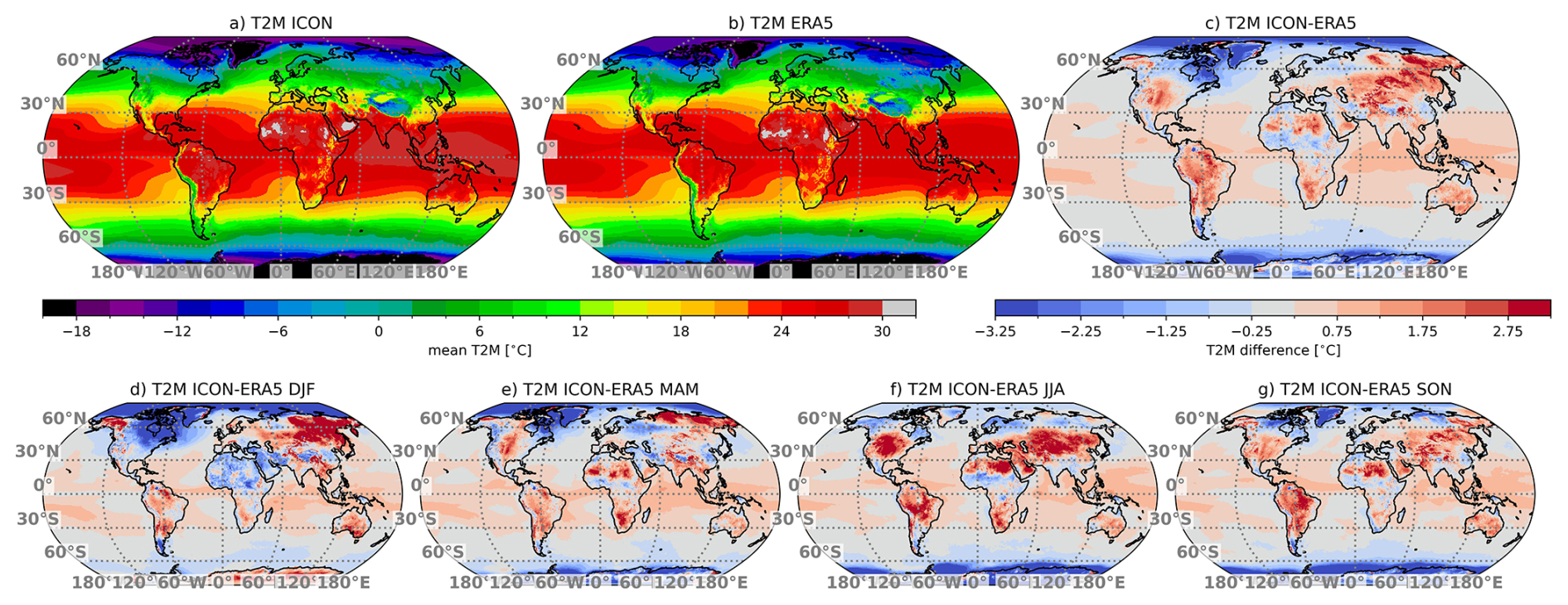
Figure 1 Annual mean daily T2M in ICON (a), ERA5 (b), and their difference (c) during the simulation period. Seasonal average T2M differences are shown in (d)–(g).

During boreal summers, temperatures exceeding 3 °C warm differences emerge in continental regions such as the central U.S. and Eurasia (Fig. 1f). Part of these differences is likely related to a misrepresentation of land-atmosphere interactions, such as the lack of lateral groundwater flow and the corresponding reduced evapotranspiration in land-atmosphere coupling hot-spots such as the central U.S., which can cool down these regions by several degrees Celsius during the summer season (Barlage et al., 2021; Schlemmer et al., 2018). Additionally, misrepresented cloud radiative forcings frequently (Fig. S1 in the Supplement) contribute to surface temperature biases in models with convection parameterizations (e.g., Ahlgrimm and Forbes, 2012) and km-scale models (e.g., Sakradzija et al., 2020; Lucas-Picher et al., 2024).

It is important to note that the differences shown here and in the following sections are partly related to the short simulation period of four years. Climate internal variability can cause large differences at local scales (Deser et al., 2012) even though observed sea surface temperatures are used.

3.2 Surface fluxes: Incoming shortwave and longwave radiation, and latent and sensible heat

Figure 2 shows the daily mean surface incoming shortwave radiation (SW_in) for (a) ICON, (b) the EWEMBI observational dataset, and (c) their difference. Overall, SW_in is underestimated over oceans, especially along the Intertropical Convergence Zone, and overestimated over land, particularly in mountainous regions. This overestimation over land is also evident when comparing the simulation to flux tower observations (Fig. 2d, e). The median difference in land mean SW_in is approximately 6.8 W m⁻², with a median difference of around 28.2 W m⁻². The overall median difference is consistent with the mean bias error of approximately 7.8 W m⁻² reported for CMIP6 models by He et al. (2023). Previous studies have shown that shallow clouds are frequently a main contributor to continental surface energy biases in km-scale models (e.g., Sakradzija et al., 2020; Lucas-Picher et al., 2024).

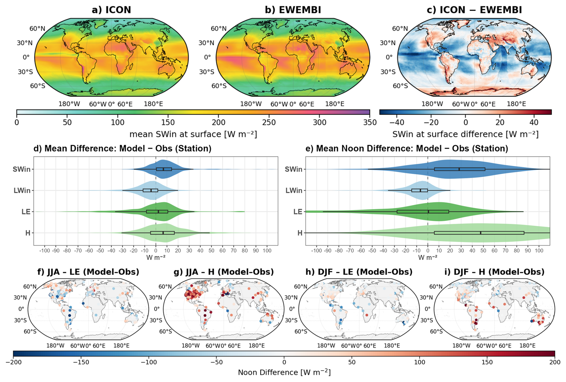
Figure 2 (a–c) Daily mean incoming shortwave radiation at the surface (SW_in) from (a) ICON (2020–2024), (b) the EWEMBI (2012–2016) observational dataset, and (c) their difference (ICON – EWEMBI). (d–e) Violin plots of station-based differences (model – observations) for mean (d) and mean local solar time noon (e) surface fluxes: SW_in, incoming longwave radiation (LW_in), latent heat flux (LE), and sensible heat flux (H). Boxes indicate the interquartile range and median difference. (f–i) Station-based mean noon differences (model -− observations) for LE and H during JJA (June, July, August) and DJF (December, January, February).

Figure 2d and e show the spatial distribution of station median total and noon differences in longwave downward radiation (LW_in), latent heat flux (LE), and sensible heat flux (H). LW_in is slightly underestimated. LE shows a median difference close to zero across stations, with regionally over- and underestimations of more than 10 W m⁻² that cancel each other on average. This spatial compensation suggests region-dependent limitations in the representation of land-surface controls on evaporation, rather than a uniform model bias. In contrast, H is more consistently overestimated, particularly during noon, agreeing with the overestimation in SW_in.

The spatial pattern of station-based mean noon differences in LE and H during JJA shows a pronounced underestimation of LE and an overestimation of H at most stations in ICON (Fig. 2f, h) in agreement with the T2M differences shown in Fig. 1. We suspect that parts of the systematic dry-summer biases are due to the absence of a lateral subsurface water-flux scheme in TERRA. Previous studies have shown that the lack of such lateral groundwater redistribution can lead to substantial surface flux and temperature biases at km-scale grid spacing (Barlage et al., 2021; Soares et al., 2024). In contrast, there is more station-to-station variability for winter biases. The spatial patterns and characteristics of surface flux differences are consistent with biases in temperature and precipitation.

3.3 Precipitation (PR)

Annual and seasonal differences between ICON and GPM-IMERG are shown in Fig. 3. The Pearson pattern correlation of annual average precipitation is 0.91 (0.87 over land cells) and the corresponding relative RMSE is 41 %. Most noticeable are wet differences over most tropical ocean regions except for the west Maritime Continent (Fig. 3c). This is consistent with the negative SW_in differences shown in Fig. 2c. Land precipitation is relatively well simulated overall, although dry differences emerge in several continental regions during boreal summer (Fig. 3g). In some of these regions, including parts of the central U.S. and Eurasia, the dry differences coincide with warm T2M differences (Fig. 1f), higher SW_in, lower LE, and higher H, suggesting a contribution from land-atmosphere coupling and cloud radiation biases.

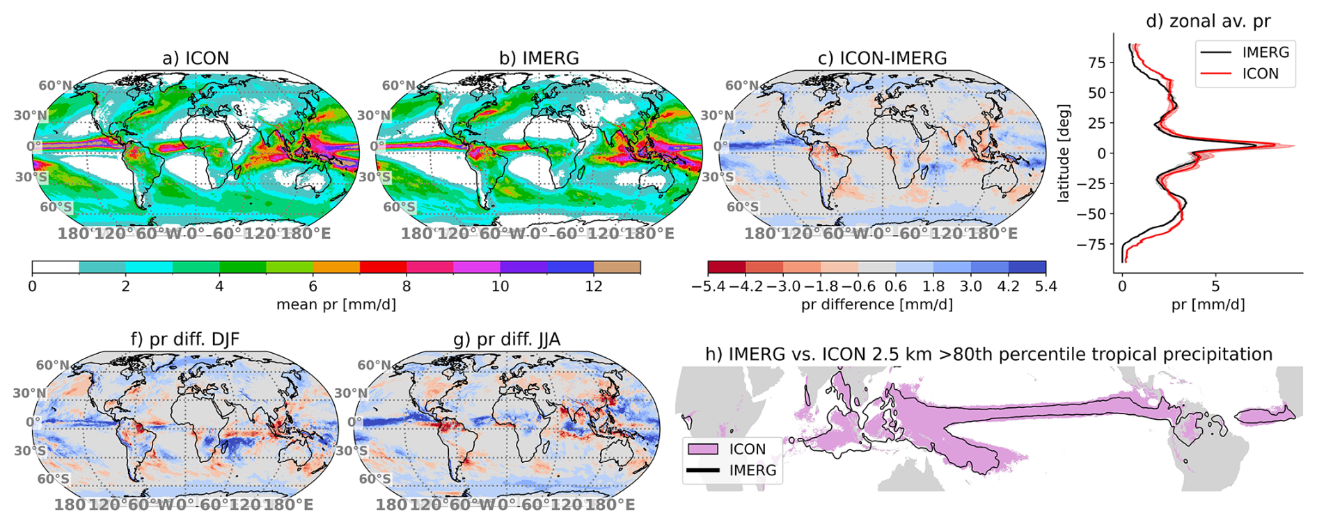
Figure 3 Annual mean daily precipitation in ICON (a), IMERG (b), and their difference (c) during the simulation period. DJF and JJA average precipitation differences are shown in (f) and (g), respectively. Mean zonal average precipitation is shown in (d) with inter-annual spread shown in contours. The area that covers the 80th percentile of tropical average precipitation (±20°) from ICON (purple) and IMERG (black contour) is shown in (h).

Zonal average precipitation agrees very well between GPM-IMERG and ICON, partly because of error cancellation effects (Fig. 3d). The differences are typically smaller than the inter-annual variability (shading in Fig. 3d) except for high-latitudes where IMERG is known to underestimate precipitation accumulations due to issues in remote sensing solid precipitation (Song et al., 2021) complicating a reliable evaluation. The location of the wet regions in the tropics (defined as the 80th percentile of tropical average precipitation; Fig. 3h) is remarkably well captured with a single tropical rainband.

This is a big achievement since simulating a realistic rainband is challenging, even at a km grid spacing, as Segura et al. (2022, 2025a, b) found a double ITCZ in the Indo-Pacific using km-scale ICON simulations with model physics different from ours. They found a lack a surface fluxes (caused by too little surface winds) in this region, which they resolved by increasing the minimum surface wind speed in the lowest model level from 1 to 4 m s⁻¹ (Segura et al., 2025a). Our model settings, which are similar to ICON's NWP setup, do not feature this issue. While it is unclear exactly what causes the differences in model performance among the ICON setups, a key difference lies in the turbulence parameterizations and surface-layer schemes, while Takasuka et al. (2024b) found large sensitivities to the formulation of microphysics. The location of mid-latitude precipitation bands associated with the storm tracks is reasonably well simulated (Fig. 3a, b).

Comparing peak hourly precipitation over the four-year evaluation period between GPM-IMERG and ICON shows that our simulation yields substantially larger values, particularly in the tropics and subtropics (Fig. 4a, b). This is predominantly caused by too low heavy hourly precipitation in GPM-IMERG since comparisons with hourly precipitation gauge observations from the HadISD dataset show that ICON reliably reproduces observed intense precipitation rates across various climate regions. At the same time, GPM-IMERG fails to capture intense rates, particularly at lower latitudes (Fig. 4c–f), which is in agreement with previous research (Guilloteau and Foufoula-Georgiou, 2020; Dominguez et al., 2024; Yu et al., 2025). However, a proper evaluation of hourly precipitation using station data is not possible in many parts of the globe due to insufficient data coverage and a lack of data sharing (e.g., Prein and Gobiet, 2017). Our presented analysis is primarily based on data from the U.S. and Europe (see Fig. S2). Results for additional climate regions, often based on only a few stations, are shown in Fig. S3.

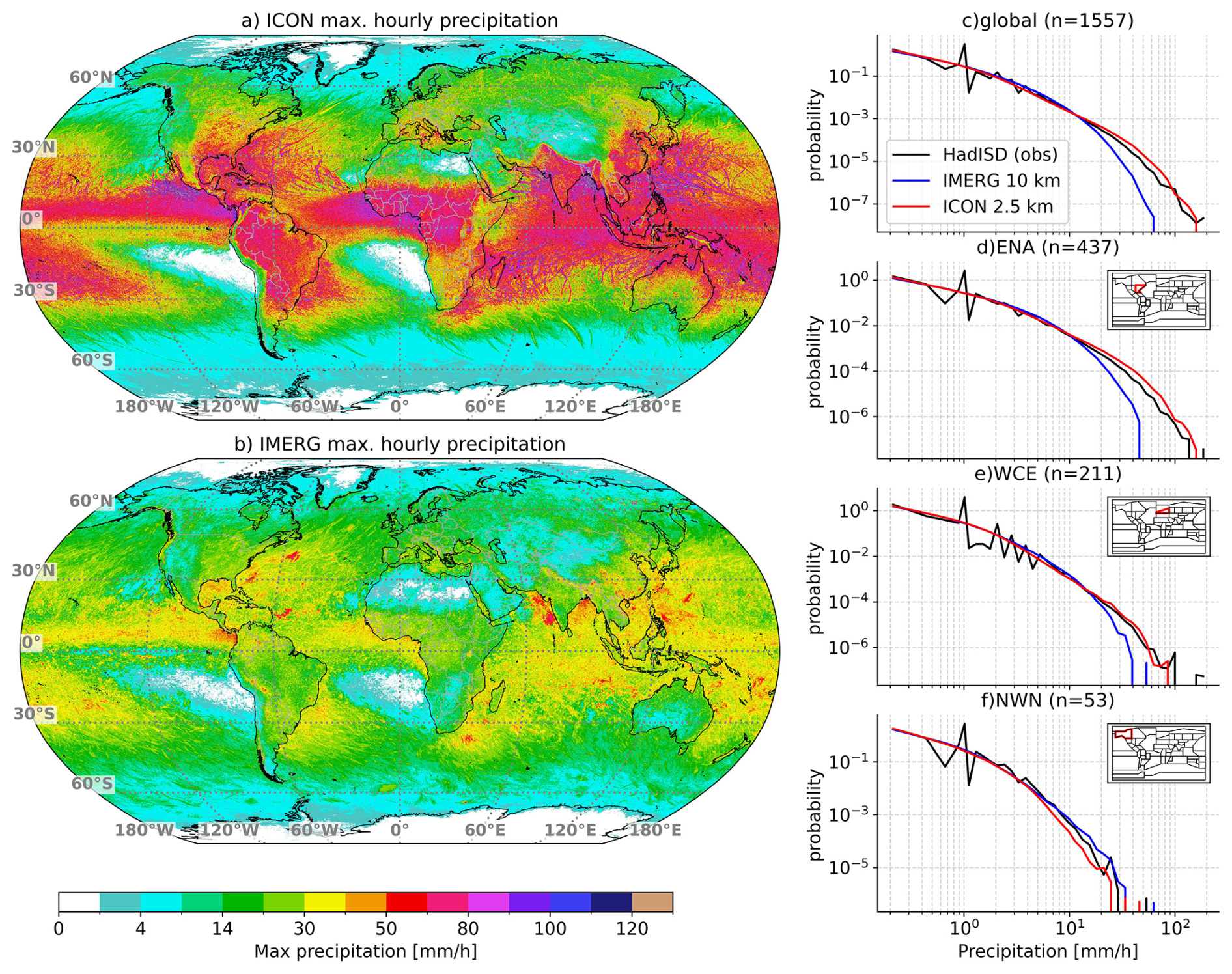
Figure 4 Hourly maximum precipitation accumulation during the simulation period from ICON (a) and IMERG (b) on the 0.1° IMERG grid. Probability density functions for hourly precipitation comparing ICON (red) and IMERG (blue) against HadISD station observations (black) globally (c) and in the Eastern North America (ENA, d), Western Central Europe (WCE, e), and North Western North America (NWN, f) region. The locations of these regions are shown in the inlet maps in (b)–(f). The underlying station density in the HadISD dataset is shown in Fig. S2.

Using the same station network, we assess the June–July–August (JJA) season-average precipitation diurnal cycle (Fig. 5; we use 0.1 mm h⁻¹ as the threshold for precipitation intensity and frequency statistics). The performance of ICON is regionally dependent and shows good agreement for capturing precipitation amount, frequency, and intensity in the North Central America (NCA) region that is heavily influenced by the North American Monsoon (Fig. 5g–i). In Eastern North America (ENA), precipitation frequency is well captured compared to station data. Still, precipitation intensity is overestimated, resulting in an overly amplified evening and nocturnal peak in precipitation amplitudes (Fig. 5a–c). Western Central Europe (WCE) shows a too-early peak in precipitation that decays too quickly. The precipitation amount is also low-biased due to the too low precipitation frequency. Generally, ICON shows greater fidelity in capturing the diurnal cycle of convective precipitation in southern regions (ENA and NCA) than GPM-IMERG.

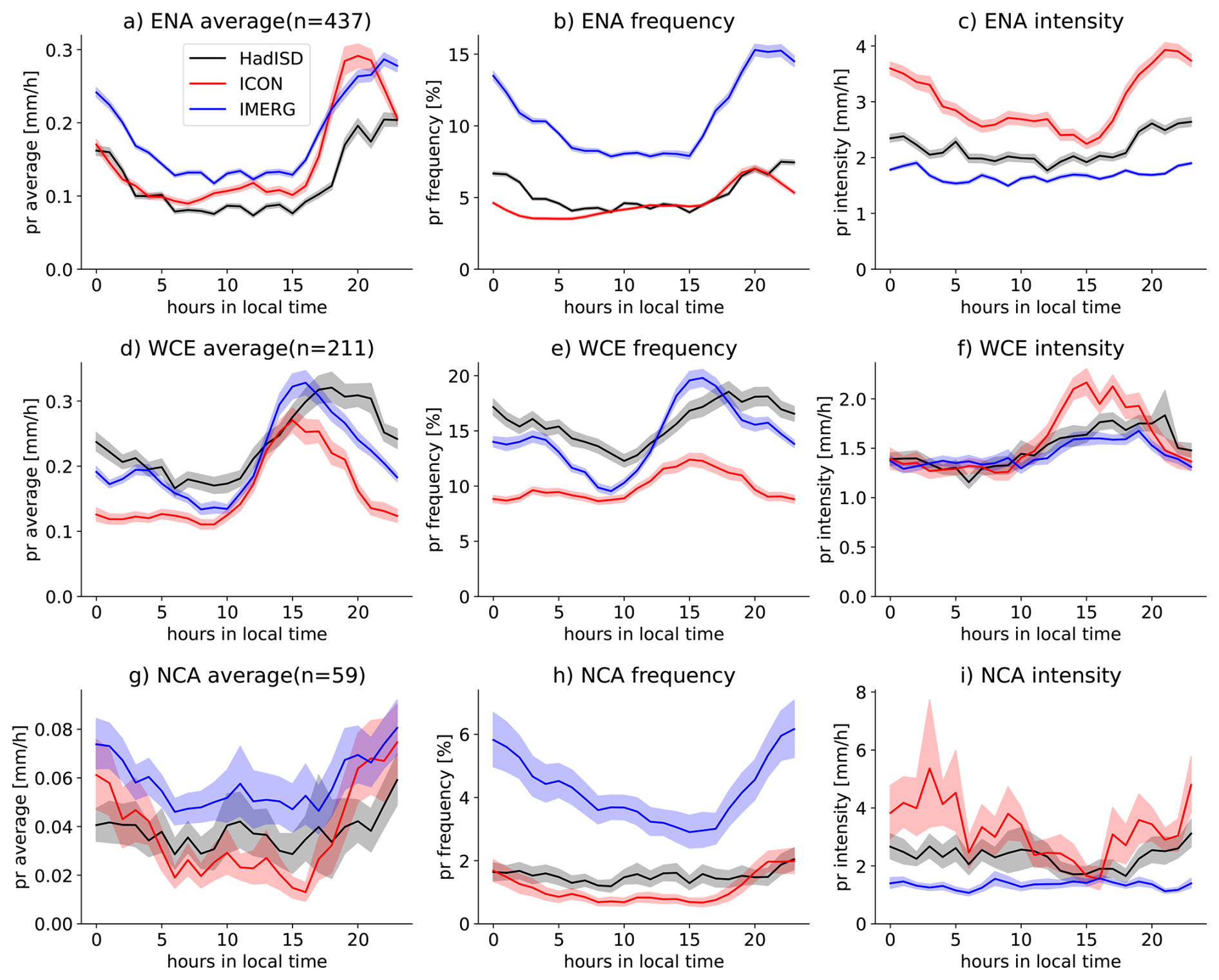
Figure 5 Hourly precipitation diurnal cycle during June, July, and August of average precipitation (a, d, g), precipitation frequency (b, e, h), and precipitation intensity (c, f, i). Results are shown for the Eastern North America (a–c), Western Central Europe (WCE), and North Central America (NCA) region. Precipitation frequency and intensity statistics are based on a precipitation threshold of ≥ 0.1 mm h⁻¹. Data are based on HadISD records (black lines) with more than 50 % coverage. Missing values in HadISD are also removed in the ICON (red ines) and IMERG (blue lines) data. Contours show station sampling uncertainties based on the 10th to 90th percentile values from 10 000 bootstrap samples (with replacement).

From Fig. 5, we see that the peak timing of convective precipitation amount is relatively well captured by GPM-IMERG, consistent with previous findings (e.g., Dominguez et al., 2024) although IMERG has been reported to have a phase lag relative to Ku-band radar in many regions which should be kept in mind (Hayden and Liu, 2021). This allows us to evaluate ICON on a near-global scale (Fig. 6). We perform this analysis during seasons dominated by convective precipitation, namely JJA at > 30° N, December–January–February (DJF) at < 30° S, and annually in the tropics. GPM-IMERG and ICON feature afternoon precipitation peaks over land. In contrast, tropical ocean regions feature predominantly nighttime and early-morning peaks. Some land regions also feature nocturnal precipitation peaks, particularly in the lee of mountain ranges (e.g., the central U.S., the La Plata basin, eastern China, and the Sahel and Western Africa), which are related to nocturnal mesoscale convective system activity. ICON can capture these nocturnal peaks reasonably well, but the spatial extent of nocturnal regions is often too small, particularly in the Amazon Basin and the central U.S. The relative amplitude of the convective precipitation diurnal cycle (diurnal amplitude divided by mean precipitation) is also relatively similar, with a tendency for larger values in ICON compared to GPM-IMERG.

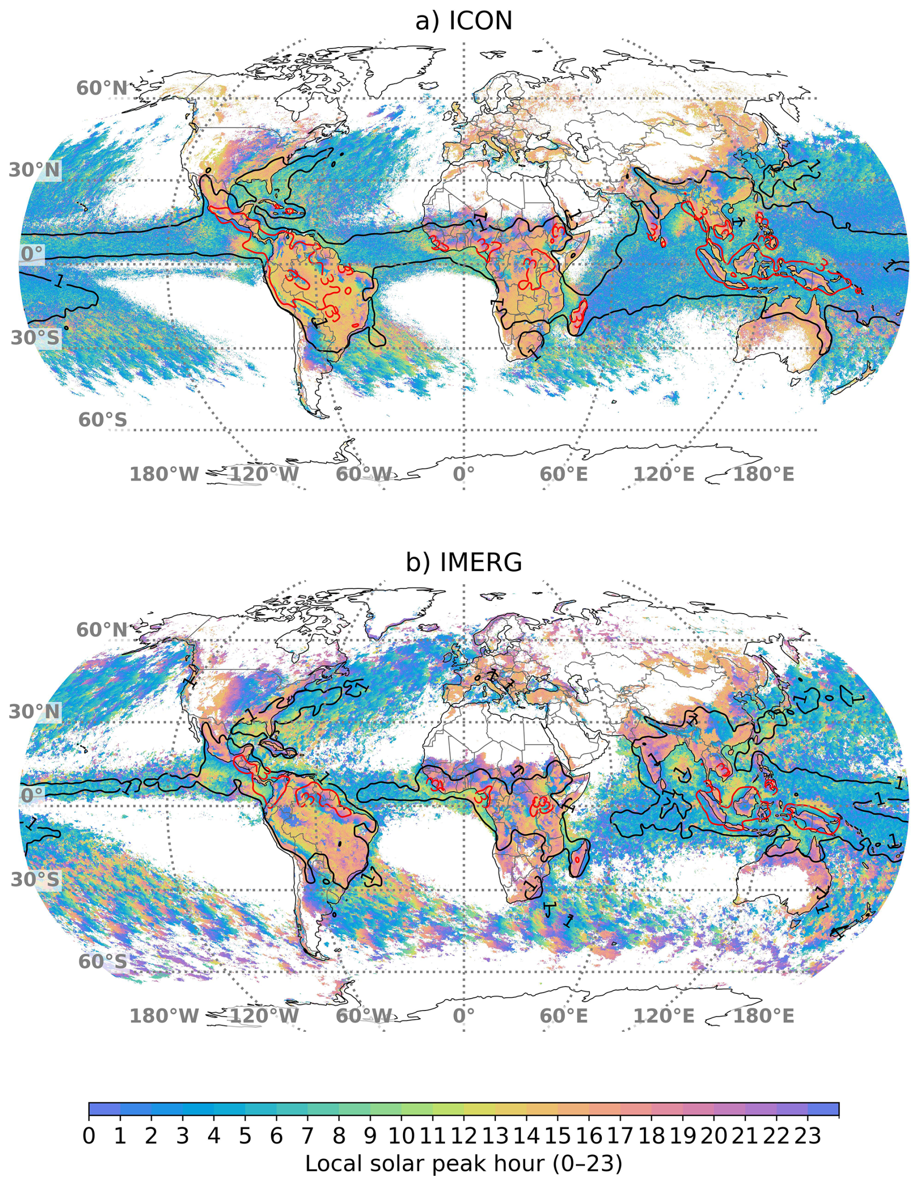
Figure 6 Color-coded local peak time of precipitation diurnal cycle in ICON (a) and IMERG (b). Colored regions show areas where the precipitation diurnal cycle amplitude is larger than 40 % of the mean precipitation. Black/red contours show regions where the amplitude is larger than 100 %/200 % of the mean precipitation. Data from all months is used in the tropics ($\le \pm \mathrm{30}\mathit{°}$), data from June, July, and August is used for latitudes >30°, and data from December, January, and February is used for latitudes $<-\mathrm{30}\mathit{°}$.

In summary, we recommend using GPM-IMERGv7 hourly precipitation with caution in model evaluation studies, given its tendency to overestimate precipitation frequency and underestimate precipitation intensity. Where possible, in-situ hourly rain gauge observations should be used.

3.4 Near surface winds (UV10)

Tropical cyclones cause the most intense UV10 extremes during the evaluation period (Fig. 7a). Storm tracks of extratropical cyclones are also clearly visible in both hemispheres. Over land, mountain regions and plateaus such as the Tibetan Plateau and the Andes stand out, as do mid-latitude plains that feature straight-line windstorms (e.g., the central U.S., the La Plata Basin, and the Sahel). Also, the coastal regions of Greenland and Antarctica feature peak wind speeds exceeding 40 m s⁻¹.

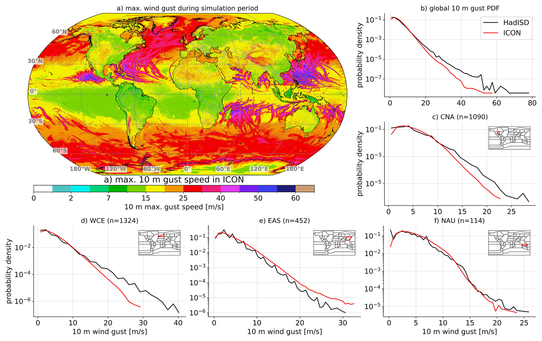
Figure 7 Maximum instantaneous simulated 10 m above surface wind from hourly model output during the simulation period (a). Probability density functions for hourly sampled winds from HadISD (black line) and ICON (red line). Statistics are shown for all stations globally (b; see Fig. S4 for station locations) and for the Central North America (CNA; c), Western Central Europe (WCE; d), East Asia (EAS; e), and North Australia (NAU; f) region. The number of stations (n) in each region is shown in the panel titles.

Evaluations against UV10 HadISD station observations show overall good agreement with a tendency of heavy wind speeds (>20 m s⁻¹) to be underestimated in ICON (Fig. 7b). However, regional differences are observed, with lower differences at high wind speeds, mostly in Mid-Latitude regions such as CNA and WCE (Fig. 7c, d). The region with the most pronounced underestimation of UV10 extremes is Eastern North America (Fig. S5), which might be partly related to a low difference in tropical cyclone frequency as we will see in Sect. 3.5, but regional differences in the simulation of extra-tropical cyclones could also contribute. Intense winds are well simulated in most tropical and high latitude areas such as East Asia (EAS) and Northern Australia (NAU) (Fig. 7e, f). The station density that is available for comparison in HadISD is shown in Fig. S4, and statistics for additional IPCC regions are shown in Fig. S6. Also, ICON reproduces the temporal autocorrelation of hourly winds well (Fig. S5), indicating that it captures the persistence and day-to-day temporal variability of near-surface wind fluctuations, including both the rapid decorrelation at short lags and the diurnal recurrence seen in the observations.

The wind speed evaluation should be interpreted with caution, as we compare station data with 2.5 km grid-cell averages. Additionally, short-term average wind speeds (e.g., 2 min averages at U.S. stations, 10 min averages at many WMO stations) are compared with hourly instantaneous model winds. Instantaneous model snapshots tend to produce broader, higher-tailed wind-speed PDFs than temporally averaged station observations, while spatial averaging over 2.5 km grid cells damps small-scale wind maxima. The combined effect partially compensates for differences. Km-scale modes are generally more comparable to station observations because the scale differences between the simulated processes on the grid and point-based observations are smaller than in coarser-resolution models.

3.5 Tropical cyclones

Tropical cyclone tracks compare well in frequency and location between ICON and IBTrACS, except for the North Atlantic Basin, which features a low bias (Fig. 8a, b). Note that the longer tracks in IBTrACS are caused by identifying TCs already as tropical depressions and following them after the extra-tropical transition. In contrast, MOAAP only identifies the main TC phase. The inter-annual variability of basin total tropical cyclone frequencies is also well captured in ICON, except for the Southwest Pacific and South Indian Ocean, where the variability is smaller (Fig. 8b).

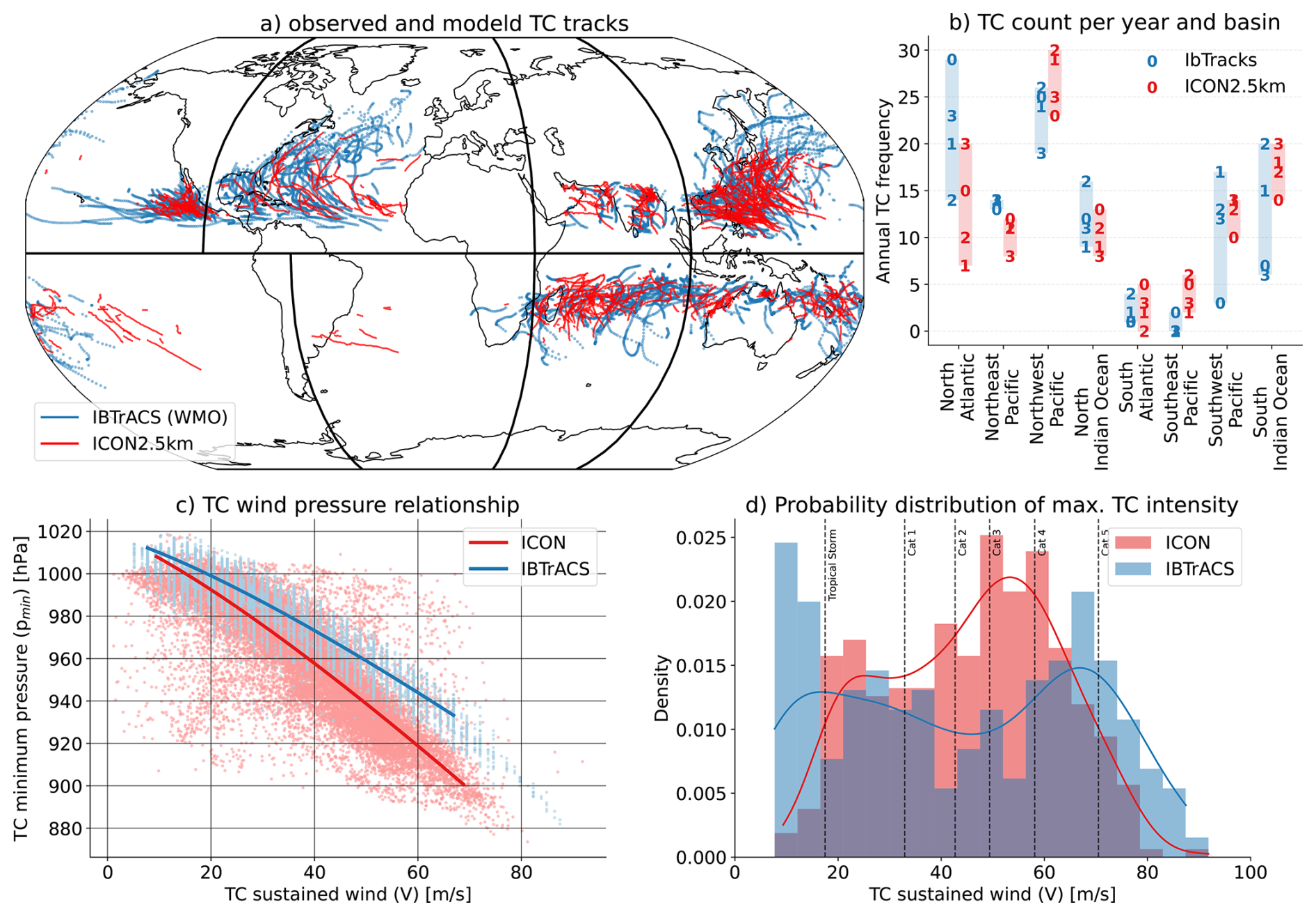
Figure 8 Tropical cyclone (TC) tracks from IBTrACS (blue) and ICON (red) during the simulation period (a). Basin annual frequency of tropical cyclones (b) in 2020 (0; only April to December), 2021 (1), 2022 (2), and 2023 (3). Tropical cyclone pressure wind relationship (c) from IBTrACS (blue) and ICON (red). Thick lines show the fitted figure of $V\left(p_{min}\right)=a(p_{\mathrm{ref}}-p_{min}{)}^b$ with p_min being the minimum cyclone pressure, V being the sustained wind speed, and p_ref being the reference pressure at zero wind speed. Probability density of lifetime peak tropical cyclone sustained wind speed in IBTrACS and ICON (d).

The TC pressure wind relationship is relatively well captured, but ICON wind speeds are too low (Fig. 8c), consistent with the UV10 analysis in the previous section and simulations with the NICAM model at km-scale (Takasuka et al., 2024a). The low difference is also reflected in the probability histogram of tropical cyclone lifetime peak wind speeds, which drops off too rapidly at high wind speeds (Fig. 8d). The IBTrACS distribution shows a bi-modal distribution with a minimum around 40 m s⁻¹ and a primary peak at low wind speeds. The reason for this primary peak is that the tropical depression and tropical storm phases of TC are included in IBTrACS. In contrast, the MOAAP tracker is calibrated to identify only storms of tropical storm intensity. Similar to the comparison to station-based wind observations in the previous chapter, comparing modeled instantaneous wind fields to IBTrACS observations is challenging. The simulation provides gridded 10 m near-surface winds, while IBTrACS reports storm-level maximum sustained winds from observational best-track analyses. They are therefore not directly equivalent, since the model resolves spatial wind structure and average wind speeds within grid cells, whereas IBTrACS summarizes cyclone intensity. This could explain parts of the low difference in wind speed seen in ICON.

3.6 Equatorial waves and the Madden-Julian oscillation

Figure 9 shows Hoffmöller diagrams of tropical average T_b in ICON and GPM-MERGIR, with labels indicating equatorial waves from MOAAP output for May 2020. While Rossby waves are well simulated in ICON, other waves that are strongly coupled to deep convection are underestimated in both frequency and amplitude. Kelvin and inertia-gravity waves (IGWs) are very infrequent, and Mixed Rossby-Gravity Waves (MRGs) are only regularly observed over Africa.

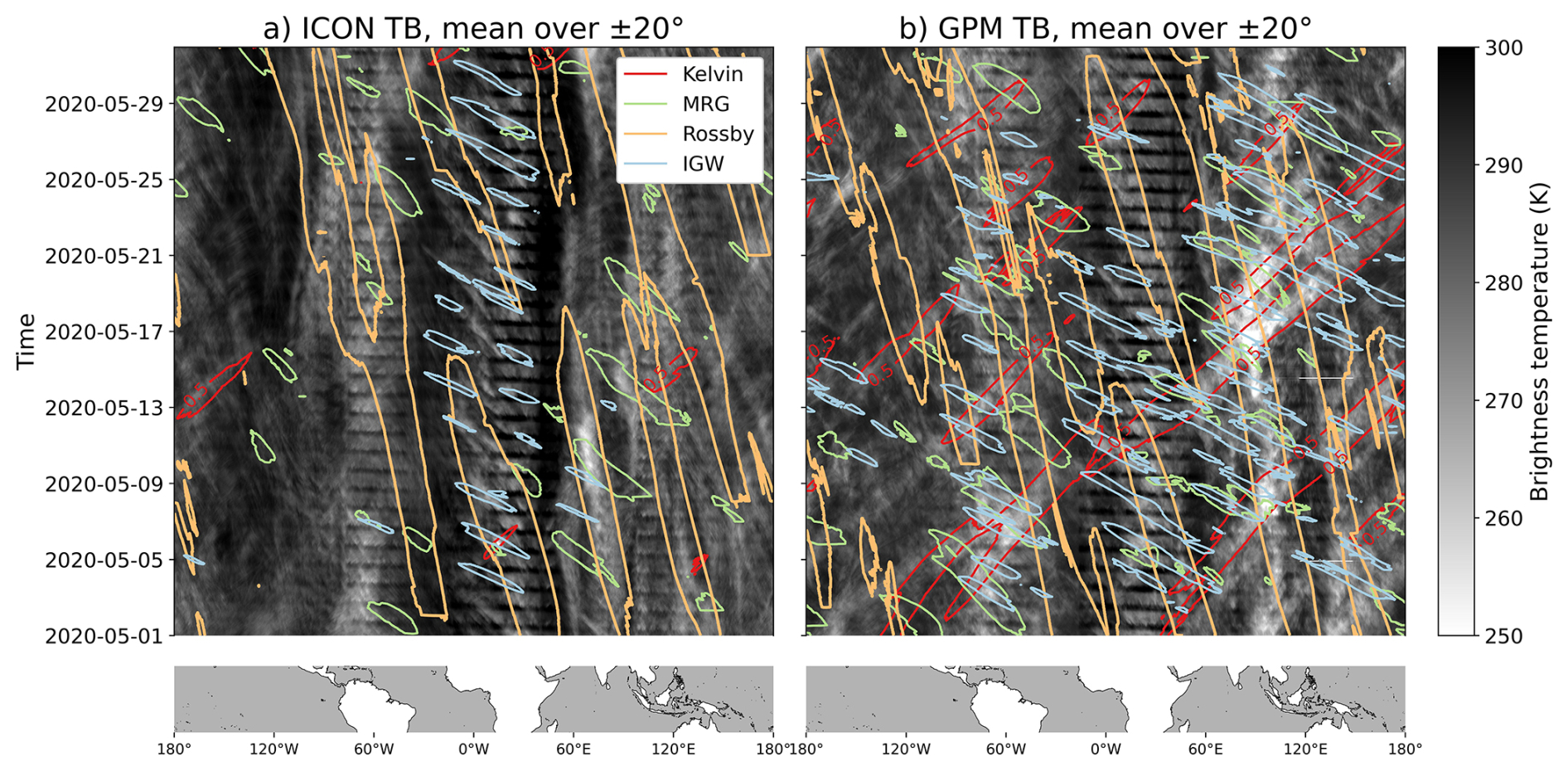
Figure 9 Hoffmöller diagrams of tropical average (±20°) brightness temperature from ICON (a) and GPM-MERGIR (b) shown in gray contours for May 2020. Contours lines show Kelvin (red), Mixed Rossby Gravity (MRG, green), Rossby (orange), and Inertia Gravity (IGW, blue) waves.

Global kilometer-scale (storm-resolving) models substantially improve the simulation of convectively coupled equatorial waves by explicitly representing deep convection, leading to more realistic precipitation spectra, wave propagation, and dynamical structures compared to models with parameterized convection (Satoh et al., 2019; Hohenegger et al., 2020; Jung and Knippertz, 2023). However, despite these advances, biases remain in wave–convection coupling strength, phase speed, and intermittency, indicating that the representation of equatorial waves at km-scale resolution is improved but still model- and configuration-dependent rather than fully resolved (Hohenegger et al., 2020; Takasuka et al., 2024a; Jung and Knippertz, 2023).

Wheeler–Kiladis space–time spectra computed from the four-year evaluation period confirm these results (Fig. 10). We follow the approach of Takayabu (1994) and Takayabu (1994), Wheeler and Kiladis (1999) and apply it to outgoing longwave radiation (OLR) from the ICON simulation and the NOAA-interpolated OLR dataset. Overall, ICON reproduces the observed spectral characteristics of equatorial waves reasonably well. Rossby wave activity shows the closest agreement with observations, while other modes – such as Kelvin waves, the Madden–Julian Oscillation (MJO), and IGW – are captured but exhibit lower amplitudes than in the NOAA OLR data.

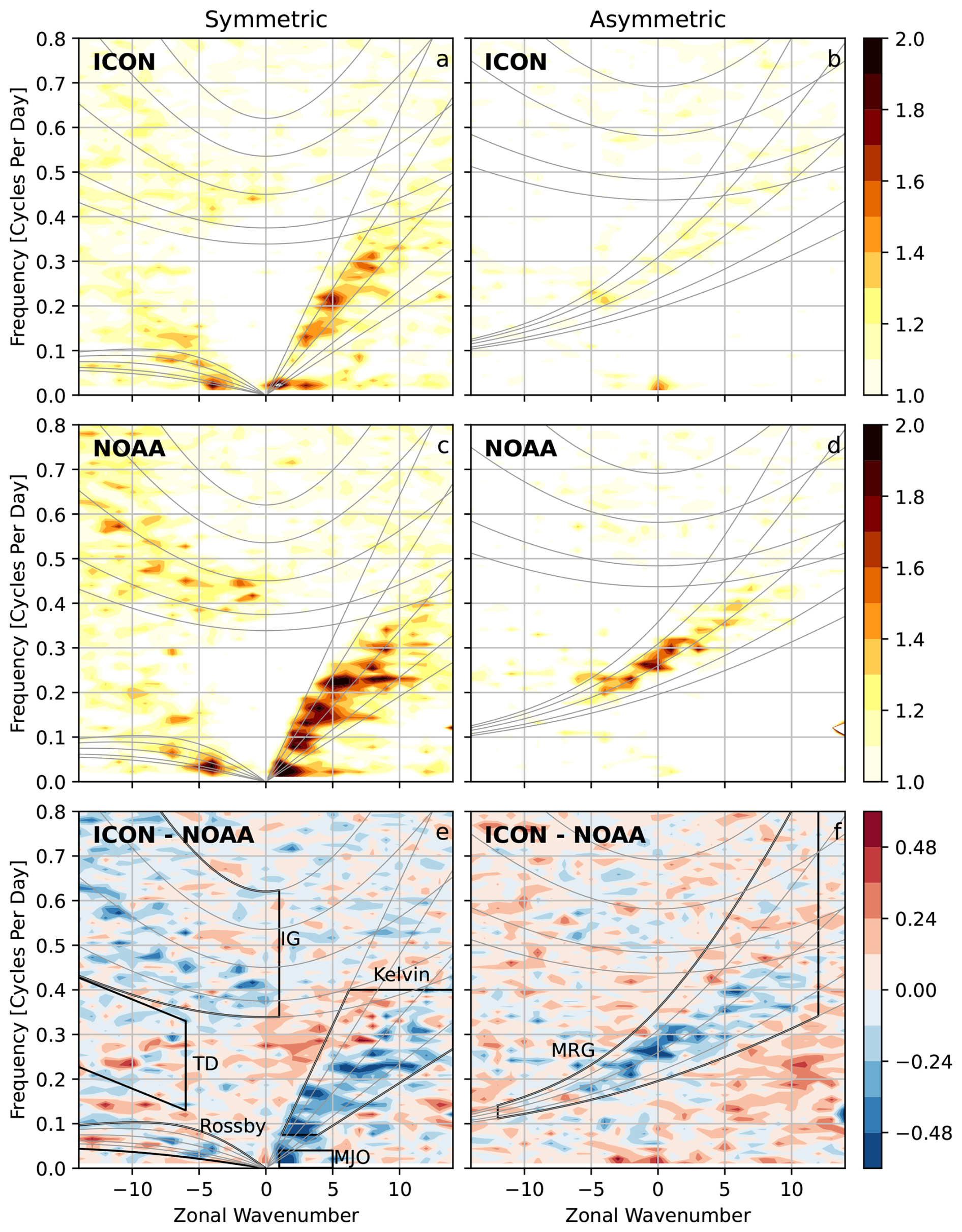
Figure 10 Wavenumber–frequency spectra of outgoing longwave radiation (OLR), divided by the background spectrum, from the ICON simulation (a, b) and NOAA satellite observations (c, d), along with their differences (e, f). Spectra are separated into symmetric (a, c, e) and antisymmetric (b, d, f) components. Gray curves indicate theoretical dispersion relations, while bold black outlines denote spectral windows associated with different equatorial wave modes: IG (inertia–gravity waves), TD (tropical depressions), Rossby, MJO (Madden–Julian Oscillation), Kelvin, and MRG (mixed Rossby–gravity waves).

3.7 Mesoscale convective systems (MCSs)

Equatorial waves often organize convection into clusters of MCSs. The latent heating from these MCSs can, in turn, amplify and sustain the wave, creating a feedback loop between the large-scale disturbance and convection (Kiladis et al., 2009). The general pattern of MCS initiation frequency is well captured in ICON, but initiation is underestimated over tropical oceans and overestimated over tropical land regions (Fig. 11a–c). The relative underestimation of oceanic MCS frequency is largest in the northern hemisphere, followed by the Southern Hemisphere, and tropics (Fig. 11g–i). In the tropics, oceanic MCS frequencies are well simulated between December and March but have a systematic low bias in the other months of the year (Fig. 11h).

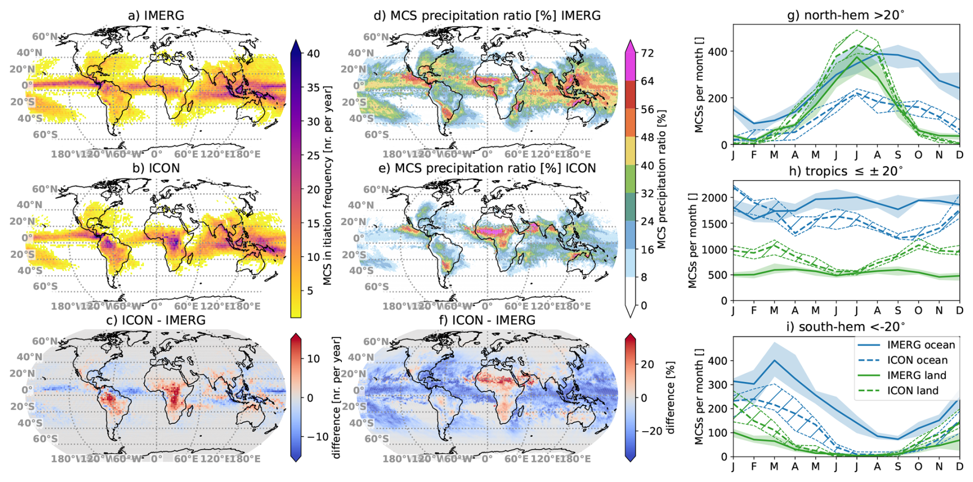
Figure 11 Annual average initiation frequency of MCSs in IMERG (a), ICON (b), and their difference. Ratio of MCS precipitation compared to total precipitation averaged over the simulation period from IMERG (d), ICON (e), and their difference (f). Monthly mean MCS frequency over land (green) and ocean (blue) in the northern hemisphere (g; >20°), the tropics (h; $\le \pm \mathrm{20}\mathit{°}$), and the Southern Hemisphere (i; <20°). IMERG results are shown with solid lines, while dashed lines show ICON results. The thick line represents the median frequency, while the contours indicate the maximum and minimum spreads over the four years.

Simulated land-based MCSs frequencies are most similar to observations in the northern hemisphere. Frequencies are overestimated in the Southern Hemisphere during summer and in the tropics year-round, except in June and July.

These frequency biases result in a systematic underestimation of the MCS to total precipitation ratio over almost all ocean regions, while this ratio is overestimated over Africa (Fig. 11d–f). The reasons for the MCS frequency biases are unclear, but they might be related to biases in tropical waves and the thermodynamic-convection coupling (Takasuka et al., 2026), which will be the topic of future research.

In addition to frequency statistics, we also performed lifetime analysis of oceanic and land-based MCSs in the tropics, northern, and Southern Hemispheres (Figs. 12 and S7 and S8 respectively). We discuss only the results from the tropics here, since they are similar in both hemispheres. Observed MCS sizes are similar over tropical oceans and land (Fig. 12a). Simulated MCSs are generally smaller than observed systems. The simulated MCS movement speed is systematically higher for most quintiles (Fig. 12b), while the mean precipitation under the MCS cloud shields is lower (Fig. 12c), particularly for land-based MCSs. Finally, modeled MCS durations are too short (2–4 h median difference), with larger differences over land than over ocean (Fig. 12d).

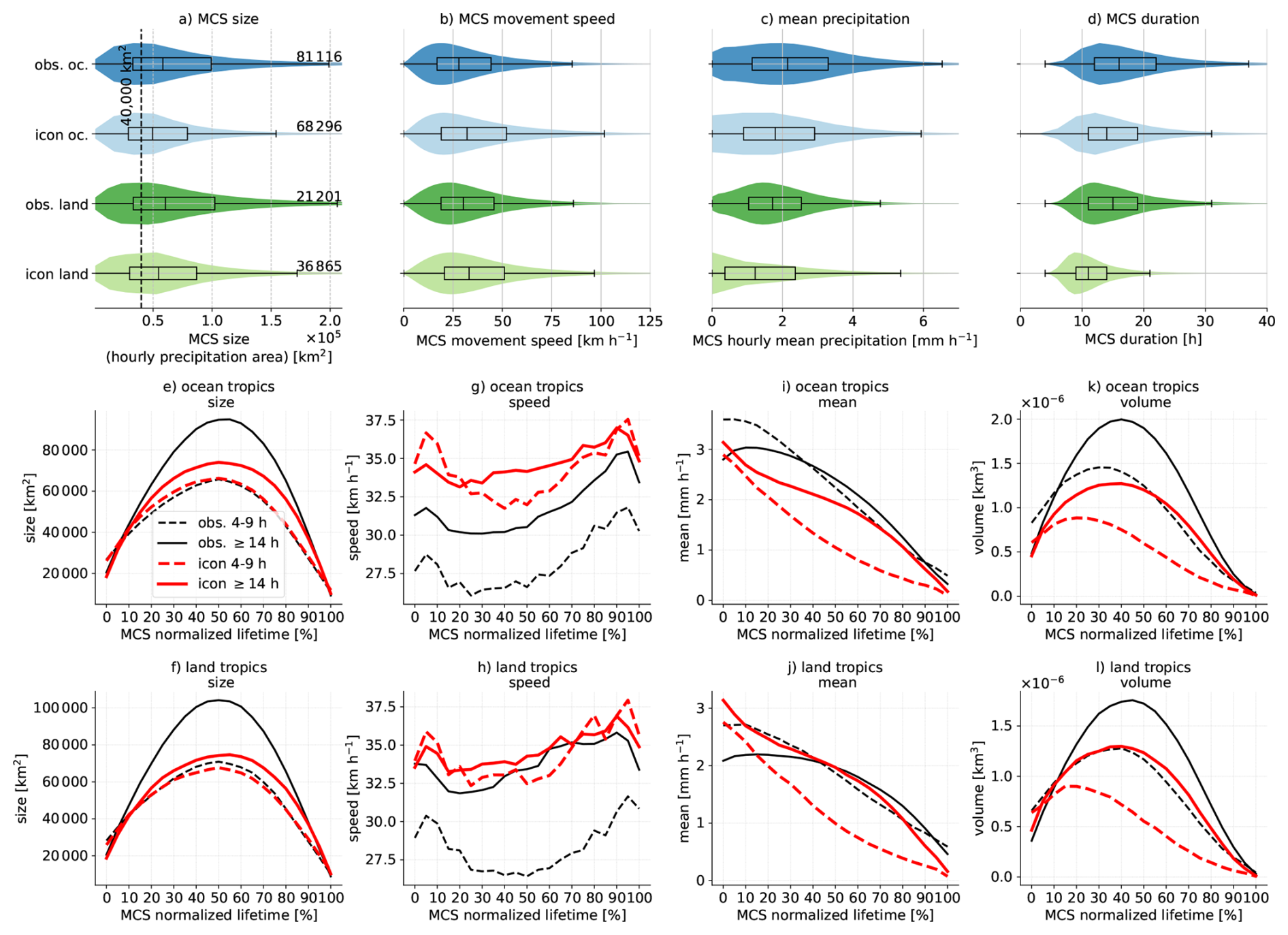
Figure 12 Violin and box-whisker plots for the distribution of tropical MCS sizes (a), speed (b), mean precipitation (c), and duration (d). The numbers right to the violins in (a) show the number of MCSs in each distribution. The lower panels show the normalized median evolution of short-lived (4–9 h; dashed) and long-lived (≥14 h; solid) MCSs in GPM observations (black lines) and in ICON (red lines). The middle panels show results for tropical oceans while the lower panel shows tropical land regions.

To compare the temporal evolution of MCSs, we differentiate between short-lived (4–9 h) and long-lived (>14 h) tropical MCSs, given lifetime-dependent model biases. The growth and decay of MCS cloud shields are well simulated for oceanic and land-based tropical MCSs (Fig. 12e, f). However, long-lived storms do not grow fast enough and reach a peak size that is about 20 %–30 % too small. On the other side, long-lived storms feature more accurate movement speeds while small storms move about 20 % too fast (Fig. 12g, h).

Mean MCS precipitation starts high during the initiation phase of MCSs and steadily decreases during their lifetime (Fig. 12i, j). This is because most MCSs start from a burst of small-scale convection and develop stratiform precipitation areas as they grow upscale until the convective areas die off in the decaying phase, resulting in mostly stratiform precipitation (e.g., Mapes et al., 2006). ICON simulates mean precipitation within ±20 % of observed values during the growth phase, with the exception of land-based long-lived systems, which show a high difference of up to 40 %. Long-lived MCSs maintain high mean precipitation rates during the growth phase of the storm (especially over tropical land), while simulated MCSs show a decline in mean precipitation even early on during their lifetime. This results in simulated mean MCS precipitation becoming increasingly low-biased over the life cycle of storms ending at low differences of up to −60 % during the decaying phase. This indicates difficulties in simulating MCS stratiform precipitation, which is a common issue in many km-scale models (e.g., Prein et al., 2023a; Zhang et al., 2024).

Finally, the combined differences in mean precipitation rates and MCS size are affecting the differences in MCS precipitation volume, which is better simulated during the growth phase but becomes increasingly negatively biased over their lifetime, especially for short-lived systems (Fig. 12k, l). The dominant driver of this bias is the low mean precipitation difference for short-lived systems, as well as the low size difference for long-lived storms. We refrain from analyzing differences in the development of heavy precipitation rates due to the deficiencies in capturing these in GPM-IMERG (see Fig. 4.)

3.8 Precipitating cloud characteristics

We found some of the largest model wet biases in tropical ocean ITCZ precipitation (Fig. 3). At the same time, MCSs are too infrequent in this region. To better understand the causes of this bias we also tracked smaller precipitating cloud systems that have cold cloud tops in addition to MCSs (see Sect. 2.3.1 and Fig. 13a–c). As previous studies have shown, cloud sizes (i.e., cold cloud top areas) follow a power-law frequency distribution (e.g., Savre and Craig, 2023). Observations show that cold cloud shields that exceed our MCS threshold (>40 000 km²) contribute the most to tropical precipitation with a maximum contribution from clouds with ∼75 000 km² (Fig. 13a). This maximum is shifted towards smaller cloud sizes and lower volumes in ICON (Fig. 13b) with a low contribution bias for large clouds and an overestimation from small clouds (Fig. 13c). Not visible in Fig. 13 are the low-frequency biases in MCSs over land and ocean, and in non-MCS precipitating cold clouds over land (Fig. S9), since only normalized distributions are shown. These results are broadly consistent with Segura and Hohenegger (2024), who showed that a large fraction of tropical precipitation originates from congestus clouds. GPM-IMERGv7 is not well suited to robustly quantify precipitation specifically from shallow or congestus clouds due to deficiencies in detecting precipitation from warm rain clouds (North et al., 2022; Huffman et al., 2023a).

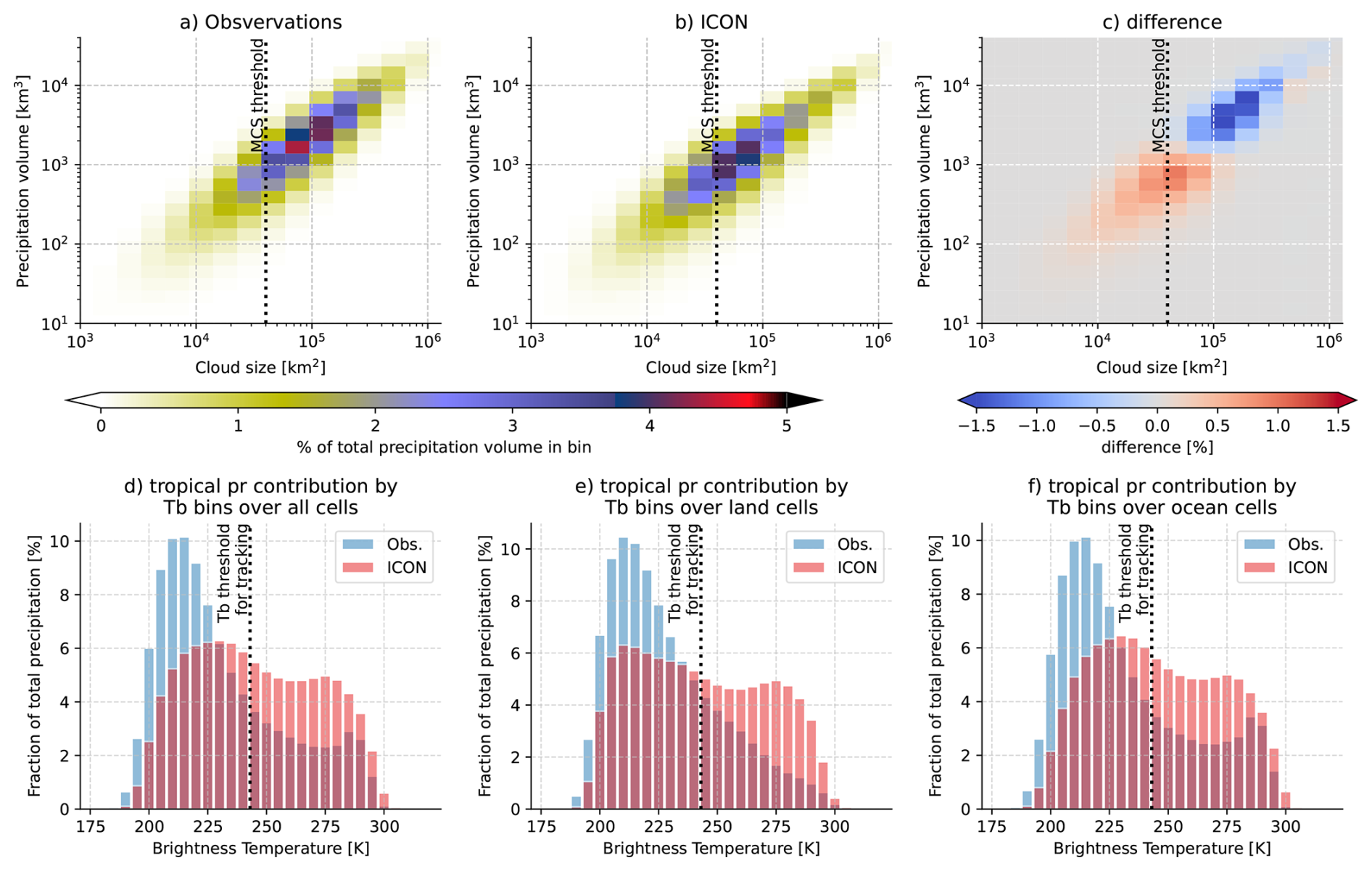
Figure 13 Relative contribution of tropical (latitude $<\pm \mathrm{20}\mathit{°}$) total precipitation from storms with cold cloud shields (T_b < 243 K) as a function of cloud shield size and precipitation volume under the cloud from observations (a), ICON (b), and their difference (c). The vertical dashed line shows the cloud shield threshold used for MCS classification. The fraction of total precipitation conditioned on T_b over the tropics (d), tropical land (e), and tropical ocean (f). The vertical dashed line shows the T_b threshold used for cold cloud identification.

A key question is: which clouds cause the excess simulated precipitation in the tropics if deep convective clouds are too infrequent and too small? Figure 13d–f show that in observations, most tropical precipitation originates beneath cold cloud tops, while ICON simulations have a too large fraction of rainfall coming from warm clouds. This issue is particularly evident in tropical land and ocean regions, but is also evident to a lesser extent in the Northern and Southern Hemispheres (Figs. S9 and S10). Excess precipitation from clouds with warm cloud tops indicates overly active warm-cloud processes, too slow glaciation in tropical clouds in the ICON microphysics scheme, or errors in GPM-IMERGv7 in capturing warm rain. This is consistent with the underestimated surface shortwave radiation over tropical oceans (Fig. 2c) that could be caused by overly reflective or overly abundant water clouds.

3.9 Drivers of heavy precipitation

The output from the MOAAP algorithm allows us to analyze the interactions among atmospheric phenomena in creating hourly heavy precipitation events in observations and in the ICON model (Fig. 14). We decided to exclude equatorial waves and fronts from the analysis in Fig. 14a–f since equatorial waves dominate tropical heavy precipitation statistics due to their large size, and including them obscures details from smaller-scale phenomena (Fig. S12). We decided to exclude fronts because they are more frequent in ICON, likely due to its higher model resolution, which allows sharper gradients to be simulated. Results including fronts and equatorial waves are shown in Fig. S12.

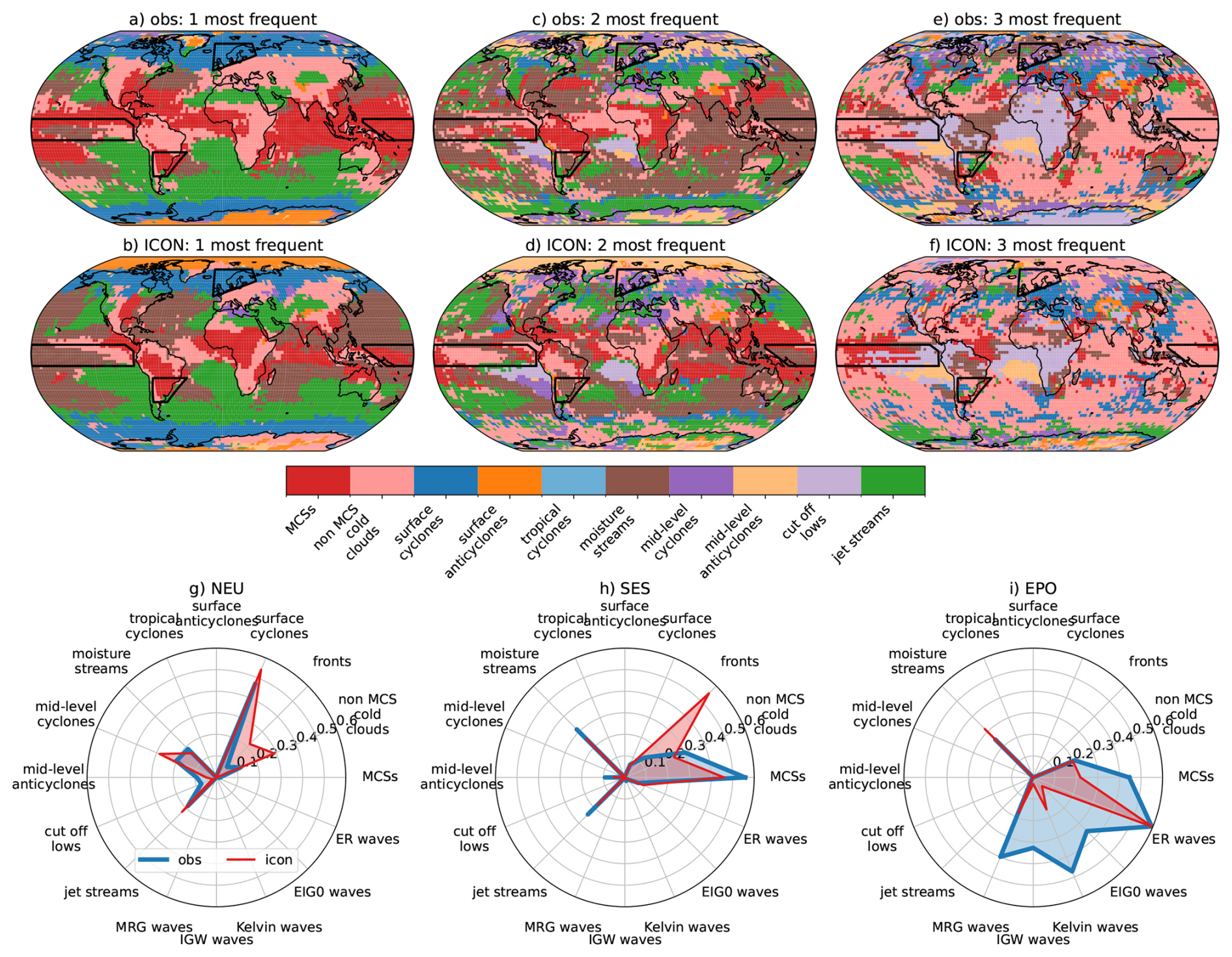
Figure 14 The most frequent (a, b), second most frequent (c, d), and third most frequent (e, f) atmospheric phenomena identified by the MOAAP algorithm that is co-located during the top 20 hourly precipitation events in the evaluation period. Observed/ICON results are shown in the top/middle panel. The data were upscaled to a 2.5° grid to reduce the signal-to-noise ratio. The same data is shown in panel (g)–(i) as the fractional frequency of the phenomenon in the Northern European (NEU), Southeast South America (SES), and Equatorial Pacific Ocean (EPO) regions (these regions are highlighted in the maps in (a)–(f)). A value of 0.5 means that 50 % of all grid cells in a region had the corresponding phenomena co-located during a heavy precipitation event.

ICON can effectively simulate the processes that cause extreme precipitation across different climate regions, though it has some notable deficiencies. In observations, MCSs are more often the most frequent producers of heavy precipitation in tropical and subtropical ocean regions (Fig. 14a, b). This agrees with our previous analysis, which showed low-frequency and size differences in simulated MCSs. In contrast, simulated MCSs are more dominant over tropical and subtropical land regions, where observations highlight non-MCS cold clouds as most important. At the same time, moisture streams (areas of low-level strong and coherent horizontal moisture transport) are frequently more relevant in ICON than in observations, particularly in subtropical ocean regions.

Figure 14g–i show frequency statistics that visualize how often a phenomenon was co-located with hourly heavy precipitation in the Northern European (NEU), Southeast South America (SES), and the Equatorial Pacific Ocean (EPO) region. In the high-latitude NEU region, observations and ICON agree that surface cyclones and mid-level cyclones are the most frequent drivers with secondary contributions from jet streams and moisture streams (Fig. 14g). ICON features more heavy precipitation events from non-MCS clouds than observed and a larger contribution of frontal systems. Cut-off lows are less frequently involved in simulated heavy precipitation events than in observations.

In the SES region, ICON agrees with observations that MCSs and non-MCS clouds are the dominant heavy precipitation-producing phenomena (Fig. 14h). ICON also captures the importance of moisture streams and jet streams well, while frontal involvement is much higher than in ERA5.

We find a relatively poor agreement in the tropical EPO region (Fig. 14i) where ICON substantially underestimates the importance of MCSs and all equatorial waves except for Equatorial Rossby waves, in agreement with previously shown results. However, ICON can capture the importance of non-MCS cold clouds and moisture streams in the production of heavy precipitation.

4 Summary and Conclusion

We present results from the first multi-year (April 2020–March 2024), global prescribed SST km-scale simulation performed with the GT4Py GPU-refactored ICON model (Dipankar et al., 2026) at a horizontal grid spacing of 2.5 km and 120 vertical levels. This experiment, conducted within the EXCLAIM project, represents a major milestone toward bridging the long-standing divide between numerical weather prediction (NWP) and climate modeling (Randall and Emanuel, 2024), using a model configuration based on operational forecasting without empirical tuning. By explicitly resolving deep convection, orographic drag, mesoscale circulations, and local land heterogeneity globally, the model enables the consistent study of weather and climate processes within a unified physical framework.

We conducted a comprehensive evaluation using satellite, reanalysis, and in-situ observations to assess the fidelity of the simulation of atmospheric phenomena at scales ranging from global to local. The following main points summarize our study:

• The ICON model reproduces observed large-scale patterns of temperature, precipitation, and surface energy fluxes with high fidelity, showing good agreement with reanalysis, satellite, and in situ observations, although biases, such as overestimation of sensible heat fluxes over land during the warm season, persist. Importantly, the model can realistically simulate the spatial pattern of tropical precipitation with a single ITCZ. However, there is an overestimation of tropical oceanic clouds (up to −40 % in incoming shortwave radiation at the surface) and precipitation (up to 50 %) and cold biases in polar regions (more than −3 °C) during winter. Additionally, warm biases over mid-latitude continents during the warm season are related to too much incoming solar radiation, an underestimation in latent heat fluxes, and an overestimation of sensible heat fluxes.

• Explicitly resolving convection yields a realistic convective diurnal cycle and an excellent representation of the hourly rainfall probability density distribution, including extremes. Still, some land regions, such as those over southern Africa, Australia, and parts of the Amazon basin, feature a diurnal precipitation peak that is too early. Importantly, model analyses that focus on the intensity or frequency of hourly precipitation should use in-situ observation records where possible, since these precipitation characteristics are not well captured in GPM-IMERG-v7 and reanalysis products, as we show here and in previous work (e.g., Dominguez et al., 2024).

• Near-surface winds and tropical cyclone statistics are generally well simulated, but maximum wind speeds are underestimated by ∼ 20 %. Tropical cyclone frequencies are well captured, except in the North Atlantic basin, where low biases are observed, similar to other high-resolution climate model simulations (Roberts et al., 2020).

• Spatial initiation patterns of MCSs are realistic, but ICON underestimates oceanic MCS frequencies (especially outside DJF) and overestimates tropical land MCSs. Simulated systems are smaller, slightly too fast, and too short-lived, resulting in an underestimation of MCS precipitation over oceans and an overestimation over some tropical land areas. The low bias in tropical MCS precipitation and the underestimation of MCS size are common among km-scale global models (Feng et al., 2025). The low-frequency bias in long-lived, large MCSs contributes to the earlier peak timing in the convective diurnal cycle.

• Since both precipitation from MCS and non-MCS cold clouds is underestimated over tropical ocean regions, it is unclear which clouds are causing the oceanic wet tropical precipitation difference in ICON. The primary cause is larger simulated rainfall from shallow and mid-level clouds (e.g., cumulus congestus) in the model. The reason for these differences is unclear, but an overactive warm-rain process in the model and deficiencies in warm-rain detection in GPM-IMERG-v7 might contribute.

• The frequency and amplitude of all equatorial waves except for Rossby waves are underestimated. This is consistent with the underestimation of MCSs and the overestimation of precipitation from shallow clouds in the tropics since equatorial waves are frequently coupled to deep convection (Kiladis et al., 2009; Prein et al., 2023b). Km-scale global models tend to capture equatorial Rossby waves well since their dynamics are more strongly controlled by large-scale vorticity gradients rather than the details of convective heating, although column water vapor also contributes (Yasunaga and Mapes, 2012; Yasunaga et al., 2019; Nakamura and Takayabu, 2022). Previous global km-scale modeling studies have shown that uncoupled models can capture convective-coupled equatorial waves (e.g., Judt and Rios-Berrios, 2021; Takasuka et al., 2024a; Ortega et al., 2026). The biases presented here might also stem in part from a misrepresentation of thermodynamic–convection coupling, which can strongly influence convective organization and its coupling to larger-scale tropical variability (Takasuka et al., 2026). Additionally, ocean-atmosphere interactions are important for simulating connectively coupled equatorial waves, which our forced SST setup does not capture (e.g., DeMott et al., 2015).

• An object-based evaluation using the MOAAP feature tracker (Prein et al., 2023b) reveals that ICON realistically captures the main meteorological drivers of heavy hourly precipitation, including cyclones, MCSs, and moisture streams. We consistently find deficiencies in simulating heavy rainfall associated with tropical oceanic MCSs and equatorial waves.

In summary, the EXCLAIM 2.5 km global ICON simulation provides a unique benchmark for studying global hydroclimatic extremes and mesoscale dynamics. It will serve as a contribution to the DYAMOND-III intercomparison initiative (Takasuka et al., 2024b), allowing for comparison with an ensemble of km-scale global models. The simulation offers novel insight into the interplay between different modes of convection and large-scale circulation. Current ICON developments within the EXCLAIM project aim to optimize the code for faster runtime and implement ocean-atmosphere coupling at km-scales (Dipankar et al., 2026). This framework also provides a basis for follow-up studies investigating how mesoscale processes, such as convective outbreaks, feed back onto and modify the larger-scale circulation. Future studies will also focus on longer integration periods, as four years are insufficient to capture climate variability.

While notable challenges remain in representing tropical variability, mesoscale convective organization, and land-atmosphere coupling, the demonstrated capability of our simulation and other km-scale global modeling efforts establishes a new foundation for next-generation Earth system modeling and the transition toward truly unified weather–climate simulations.