Why does the signal-to-noise paradox exist in seasonal climate predictability?

Estimates of the potential predictability limit (PPL) for seasonal climate, typically based on a perfect model framework, sometimes encounter challenges of being paradoxical, as actual skill surpasses the PPL. The signal-to-noise paradox (SNP) gets its name from the use of model-based signal-to-noise ratios to estimate the PPL. Here, we study seasonal climate predictability in the tropical and subtropical regions during the boreal summer (June to September), with a focus on the SNP. We estimate PPL within the perfect model framework, only considering error growth from initial conditions. Signal and noise components display temporal non-orthogonality and a weak association between estimates of PPL and actual prediction skill, contradicting its intended purpose. A significant correlation between signal and noise violates the perfect-model framework. Moreover, paradoxical regions show no clear correspondence with signal–noise correlation, indicating that while accurate signal–noise separation is necessary, it is not sufficient to eliminate paradoxes.

We have also demonstrated that sub-seasonal components, which are building blocks of seasonal mean, substantially contribute to seasonal anomalies in association with major global predictors. The co-variability between sub-seasonal components and seasonal anomalies is wide-ranging and often skewed compared to observations, thereby influencing seasonal prediction skills and PPL. Therefore, a robust PPL estimation should consider errors from initial conditions and model-related factors such as physics, dynamics, and numerical methods. In this context, we present a simple diagnostic approach to estimate the maximum achievable seasonal prediction skill, which may be interpreted as an empirical upper bound of skill or the PPL.

1 Introduction

Seasonal climate prediction plays a pivotal role in making policy decisions, facilitating long-term planning, and implementing mitigation strategies, ultimately contributing to the development of a climate-resilient society. The emergence of the first computer in the 1950s initially fostered optimism for achieving precise weather and climate prediction. However, studies by Lorenz (1963, 1969) pointed out the inherent unpredictability of weather beyond a limited temporal horizon of only a few days. Consequently, this revelation led to the perception that the endeavour of seasonal prediction was considered unattainable. Nevertheless, a significant advancement in our understanding of long-lead predictability in the tropical climate was achieved by Charney and Shukla (1981), with further elaboration by Shukla (1998). In this context, the predictability of seasonal climate is attributed to the influence of slowly evolving boundary conditions, such as sea surface temperature (SST) and soil moisture, which retain memory and significantly influence atmospheric instabilities on longer timescales. This breakthrough has established the scientific foundation for seasonal climate prediction.

While significant advancements have been made in improving the accuracy of weather forecasts over the past few decades (e.g., Bauer et al., 2015), the task of providing reliable seasonal predictions remains a formidable challenge. The Indian summer monsoon serves as an illustrative example, as attempts to predict it date back a century (Walker, 1924; Mooley and Parthasarathy, 1984), yet achieving consistently accurate seasonal forecast across all years remains challenging (Shukla, 2007; Jain et al., 2019). In addition to evaluating current prediction skills, it is of equal importance to ascertain the inherent constraints of seasonal climate predictability, denoted as the Potential Predictability Limit (PPL). It is commonly assumed that the PPL represents an upper limit on forecast skill, beyond which further enhancements become unattainable and, that a dynamical prediction system cannot surpass this limit (Kumar et al., 2005; Rajeevan et al., 2012). However, several studies have documented instances where a model's seasonal prediction skill surpasses the estimated PPL (e.g., Kumar et al., 2014; Saha et al., 2016a; Scaife and Smith, 2018), giving rise to a signal-to-noise paradox (SNP), a situation where the proportion of predictable variance in models is too weak. This translates into actual skill (correlation skill between ensemble mean and observation) being greater than the estimated PPL.

In real-world forecasting, predictability is limited by two primary sources of error: uncertainties in the initial conditions, and model errors (arising from imperfect physics, dynamics, and numerical schemes), which grow nonlinearly with time. The perfect-model framework, however, neglects model errors by construction and considers only initial-condition uncertainty, thereby providing an idealized upper bound on predictability (i.e. PPL). Within this framework, inter-ensemble spread is assumed to arise solely from initial-condition uncertainty and is treated as the noise component, while deviations of the ensemble mean from the climatological mean are interpreted as the signal component. In practice, however, model's error can contribute to both signal and noise, which potentially could giving rise to SNP, where the realized forecast skill becomes greater than the estimated PPL.

In previous studies, attempts to estimate the potential predictability of seasonal climate were predominantly focused on shorter hindcasts and employed various estimation methods (Yang et al., 2012; Scaife et al., 2014; Saha et al., 2016b, a, 2019). However, recent studies have highlighted the pervasive challenge of the SNP, which extends across different climate models and temporal scales (Strommen and Palmer, 2019; Zhang and Kirtman, 2019; Zhang et al., 2021; Sévellec and Drijfhout, 2019). Intriguingly, about 70 % of the globe exhibits SNP in annual surface air temperature simulated by CMIP5 models (Sévellec and Drijfhout, 2019). This paradox is not solely attributed to issues with initialization processes (Zhang and Kirtman, 2019; Cottrell et al., 2024). Addressing the low signal-to-noise ratio present in models has been recognized as a potential solution to improve model future projections (Smith et al., 2020). Model's response to external radiative forcing and limited ensemble size may also be responsible for SNP (Klavans et al., 2021). Nonetheless, another study utilizing the Lorenz 1963 model (Lorenz, 1963) argues that the paradox can arise from the initialization process, wherein the initial ensemble spread (standard deviation) surpasses the observational spread (Mayer et al., 2021). Large ensemble sizes and the application of post-processing techniques also hold promise for enhancing prediction accuracy by reducing noise and enhancing forecast variance (Eade et al., 2014; Smith et al., 2019). Hu et al. (2021) have shown that in NCEP CFSv2, the spatial pattern of the primary mode of signal and noise components for SST coincides over the tropical Pacific, yet their temporal variability remains uncorrelated. Moreover, the non-stationary nature of the climate system and smaller sample size (i.e. ensemble member and number of years) can confound the detection of the paradox (Weisheimer et al., 2018).

This study aims to explore the SNP in the context of seasonal prediction skill and sub-seasonal variability within tropical and subtropical regions, with a specific emphasis on South Asia and the central Pacific from June to September (JJAS). We estimate the PPL using traditional methods and assess correlation skill of rainfall, surface temperature, sea surface temperature, and mean sea level pressure (MSLP). Subsequently, we apply these methods to identify regions where the paradox exists. While the estimation methods of PPL are rooted in the idealized notion of a perfect model framework, where the model itself is considered flawless, but errors in the initial conditions result in divergence (i.e., simulations deviate with minor perturbations in initial conditions), it is essential to acknowledge that dynamical models are inherently imperfect, and the realization of a perfect model is improbable. Furthermore, estimates of PPLs are often very close to actual forecast skill and are expected to increase with advancements in the model. This raises critical questions regarding the overall usefulness of PPL. In this context, we posit that the signal and noise components in seasonal mean are not solely attributed to errors in the initial conditions but also to inadequate representation of physical processes and their associated non-linear feedback mechanisms within a dynamical model. We demonstrate a substantial contribution of sub-seasonal components to the overall variability and predictability of seasonal climate. Additionally, we identify a systematic error in the co-variability between sub-seasonal components and seasonal anomalies, which affects the accuracy of seasonal climate predictions and predictability.

Here, we introduce a diagnostic method to estimate the maximum attainable seasonal prediction skill within the available ensemble members. To account for the constraints imposed by a finite sample size (52 ensemble members over 41 years), we employ a bootstrap resampling technique to infer the true population statistics. The resulting correlation estimate may be interpreted as the upper limit of achievable prediction skill, or the PPL. Detailed data and methods are provided in Sect. 2, while Sect. 3 presents the study's results, and Sect. 4 summarizes the findings.

2 Data and methods

2.1 Model and experiments

The modified version of the Climate Forecast System version 2 (CFSv2; Saha et al., 2014a, b, 2017; Hazra et al., 2017; Sujith et al., 2019; Rai et al., 2019) of the National Centers for Environmental Prediction (NCEP) is used in this study. The CFSv2 consists of a spectral atmospheric model (i.e. Global Forecast System) at a horizontal resolution of about 1° (i.e. T126) with 64 hybrid vertical levels and the GFDL Modular Ocean Model version 4p0d (Griffies et al., 2004) with 40 vertical layers and 0.25–0.50° horizontal grid spacing. The CFSv2 is coupled with a two-layer sea ice model (Wu et al., 1997; Winton, 2000) and land surface model Noah with four layers of soil and single layer snow scheme (Ek et al., 2003).

As CFSv2 shows a maximum (minimum) skill in Indian summer monsoon rainfall (ISMR) with February and April (March and May) initial conditions (e.g., Saha et al., 2016a; Pokhrel et al., 2016), based on NCEP's Climate Forecast System Reanalysis (CFSR; Saha et al., 2010), February initial conditions are used to generate ensemble re-forecasts/hindcasts for the years 1981–2021. The model (00:00, 06:00, 12:00, and 18:00 GMT). Therefore, 52 ensemble member simulations are performed, each year spanning 9-months.

2.2 Observed data

In this study, we employ multiple observed/reanalysis data sets for analysis and comparisons with model simulations. Over land, 2 m air temperature data from the Climatic Research Unit (CRU TS3.1; Harris et al., 2014) is used. SST data is taken from EN4 reanalysis (Good et al., 2013). MSLP data is obtained from ERA5 reanalysis (Hersbach et al., 2020). Daily rainfall data from the Global Precipitation Climatology Project (GPCP Version 1.3, 1°×1°; Huffman et al., 2001) for 1997–2021 and monthly rainfall data from GPCP version 2.3 (Adler et al., 2020) for 1979–2021 with 2.5°×2.5° horizontal resolution are employed.

2.3 Methodology

Here, we employ the Analysis of Variance (ANOVA) method based on the perfect model framework (e.g., Rowell et al., 1995; Rowell, 1998; Schneider and Griffies, 1999) to estimate PPL. The PPL serves as a measure of the model's ability to predict the Earth's weather and climate with the utmost skill, where prediction skill should always be lower than the PPL due to unavoidable errors in the initial conditions. However, it is found that the prediction skill of a model is higher than the PPL on several occasions and across the globe, which is termed as SNP. Furthermore, to verify the existence of SNP, the Ratio of Predictable Components (RPC) is used (Eade et al., 2014).

2.3.1 ANalysis Of VAriance (ANOVA) method

To quantify the intrinsic predictability of the climate system, we adopt a framework based on large ensemble simulations, which allows a clear separation between predictable and internally generated variability. By performing multiple realizations with slightly different initial conditions, it becomes possible to isolate the deterministic component of variability from stochastic fluctuations. In this context, the ensemble mean represents the predictable signal associated with large-scale forcing, while deviations from this mean reflect internal variability arising from chaotic processes (e.g., Rowell et al., 1995). This separation provides a physically meaningful basis for estimating the upper bound of predictability, independent of forecast skill. Building on this conceptual framework, the total variance can be formally decomposed into signal and noise components using the ANalysis Of VAriance  NOVA) approach, as described below.

In this method, the total variance is split into signal (${\mathit{\sigma }}_{\mathrm{sig}}^{\mathrm{2}}$) and noise (${\mathit{\sigma }}_{\mathrm{noise}}^{\mathrm{2}}$) components. The variance decomposition framework of the ANOVA methodology introduced by Rowell et al. (1995, p. 699), which is used in several previous studies (e.g., Kang and Shukla, 2006; Saha et al., 2016a; Scaife and Smith, 2018; Weisheimer et al., 2018), is employed here. The ratio of signal to noise variance is known as the signal-to-noise ratio (SNR). If “x” is the precipitation field of the model, “i” is the year of the model integration (total year “N”), and “j” is the number of ensemble simulations (total ensemble n=52), then noise variance following Rowell et al. (1995), can be expressed as

$$\begin{array}{}\text{(1)}& {\mathit{\sigma }}_{\mathrm{noise}}^{\mathrm{2}}={\displaystyle \frac{\mathrm{1}}{N(n-\mathrm{1})}}\sum _{j=\mathrm{1}}^n\sum _{i=\mathrm{1}}^N{\left(x_{ij}-\stackrel{\mathrm{‾}}{x_i}\right)}^{\mathrm{2}}\end{array}$$

where $\stackrel{\mathrm{‾}}{x_i}=\frac{\mathrm{1}}{n}\sum _{j=\mathrm{1}}^n{x}_{ij}$ is the ensemble mean of the model for a year and the degrees of freedom is N(n−1). The variance of ensemble mean (${\mathit{\sigma }}_{\mathrm{EV}}^{\mathrm{2}}$) can be estimated as

$$\begin{array}{}\text{(2)}& {\mathit{\sigma }}_{\mathrm{EV}}^{\mathrm{2}}={\displaystyle \frac{\mathrm{1}}{(N-\mathrm{1})}}\sum _{i=\mathrm{1}}^N{\left(\stackrel{\mathrm{‾}}{x_i}-\stackrel{\mathrm{‾}}{\stackrel{\mathrm{‾}}{x}}\right)}^{\mathrm{2}}\end{array}$$

where $\stackrel{\mathrm{‾}}{\stackrel{\mathrm{‾}}{x}}=\frac{\mathrm{1}}{Nn}\sum _{j=\mathrm{1}}^n\sum _{i=\mathrm{1}}^N{x}_{ij}$ is the average over all year and all ensemble. However, the variance of the ensemble mean is often an overestimation of signal variance (Scheffe, 1959). As the number of ensemble members is not very large (here 52), the ensemble mean contains residual noise component of the variability. Therefore, the signal variance may be estimated following Scheffe (1959) as

$$\begin{array}{}\text{(3)}& {\mathit{\sigma }}_{\mathrm{sig}}^{\mathrm{2}}={\mathit{\sigma }}_{\mathrm{EV}}^{\mathrm{2}}-{\displaystyle \frac{\mathrm{1}}{n}}{\mathit{\sigma }}_{\mathrm{noise}}^{\mathrm{2}}.\end{array}$$

Therefore, the total variance can be estimated as

$$\begin{array}{}\text{(4)}& {\mathit{\sigma }}_{\mathrm{TV}}^{\mathrm{2}}={\mathit{\sigma }}_{\mathrm{sig}}^{\mathrm{2}}+{\mathit{\sigma }}_{\mathrm{noise}}^{\mathrm{2}}.\end{array}$$

The signal variance arises due to slowly varying quasi-periodic or aperiodic boundary conditions, such as El-Niño Southern Oscillation (ENSO), which evolve on a longer time scale than the predictand (e.g. seasonal monsoon rainfall). In general, the power associated with quasi-periodic slowly evolving processes is higher than that of faster-evolving processes (Peixoto and Oort, 1992, Fig. 2.7). Hence, the slowly evolving process may dictate the evolution of the faster processes, contributing to predictability. The ratio of signal to noise variance (a quantitative measure of predictability) is known as the signal-to-noise ratio (or SNR). A perfect coupled model does not attest to a perfect seasonal rainfall forecast due to unavoidable errors in the initial conditions. Therefore, there will always be an upper limit to the seasonal predictability (e.g., Kang and Shukla, 2006; Westra and Sharma, 2010), which can be expressed in terms of SNR as

$$\begin{array}{}\text{(5)}& {\mathrm{PPL}}_{\mathrm{ANOVA}}=\sqrt{{\displaystyle \frac{\mathrm{SNR}}{\mathrm{SNR}+\mathrm{1}}}}.\end{array}$$

The values of PPL vary between 0 and 1 and show the maximum limit of correlation skill achievable by a model at a given lead time.

2.3.2 Ratio of Predictable Components (RPC)

RPC method (Eade et al., 2014) is used to identify the signal-to-noise paradox. The RPC is the ratio of predictable components in observation to that in the model. The predictable component in observation (PC_obs) is estimated directly from the fraction of the variance that can be explained by model forecasts (i.e. correlation). The predictable component in the model (PC_model) is estimated by the ratio of the variance of the ensemble mean to the variance of individual ensemble members. Ideally, RPC should be 1, as the observation and model should contain the same proportion of predictable variance, and the squared correlation should match the predictable proportion of variance in the model. Regions where the RPC index is greater than 1, show that the predictable component in the model is less than that we see in the real world (i.e. paradox). The RPC is given by

$$\begin{array}{}\text{(6)}& \mathrm{RPC}={\displaystyle \frac{{\mathrm{PC}}_{\mathrm{obs}}}{{\mathrm{PC}}_{\mathrm{mod}}}}\ge {\displaystyle \frac{r}{\sqrt{{\mathit{\sigma }}_{\mathrm{noise}}^{\mathrm{2}}/{\mathit{\sigma }}_{\mathrm{TV}}^{\mathrm{2}}}}}.\end{array}$$

2.3.3 Projection of sub-seasonal variance on seasonal anomaly

Unlike variables such as temperature or surface pressure, which vary smoothly in time, rainfall is inherently discrete and typically occurs in pulses (rain or no-rain) concentrated within preferred time bands (i.e., sub-seasonal bands). Furthermore, the amplitude of these events in the tropical monsoon region is often much larger than that of the annual cycle (Fig. S1 in the Supplement). As a result, variations in sub-seasonal rainfall can significantly modify the annual cycle or seasonal anomaly. This can be easily demonstrated by removing just one or 2 d of rainfall from daily time series over core monsoon region. Upon removal of 2 d rainfall event (>80 mm d⁻¹; red bar in Fig. S1), assuming it arises from sub-seasonal variability, the reconstructed annual cycle, becomes visibly weaker, with decrease in seasonal anomaly by 59 % of its interannual standard deviation. It may be noted that only two snigle-day rainfall events are removed here; if a complete event is removed, as happens, the impact on the seasonal anomaly would be substantially larger. This highlights why sub-seasonal components are often termed the “building blocks” of the monsoon. The seasonal mean precipitation is simply the sum of precipitation during these events. Moreover, various sub-seasonal bands contributed differently to the seasonal anomaly (Fig. S2). As the sum of these sub-seasonal events forms the seasonal mean, year-to-year variability in the characteristics of sub-seasonal components also contributes to seasonal anomalies. In other words, global predictors affect seasonal precipitation by modulating sub-seasonal components, such as changing the intensity and duration of these events (e.g. Saha et al., 2019, 2020, 2021).

Due to imperfections in model physics, accurately simulating sub-seasonal components remains a challenge. Therefore, their anomalous contributions to seasonal anomalies are problematic. For example, in the Indian summer monsoon, synoptic systems (i.e., lows and depressions) contribute about 45 %–55 % of the seasonal mean precipitation (e.g. Yoon and Chen, 2005), and account for the maximum year-to-year variability (Saha et al., 2020). Therefore, errors in the co-variability between seasonal mean and sub-seasonal variance can also contribute to ensemble spread. To demonstrate this, we analyzed the seasonal variance of prominent sub-seasonal bands in the rainfall time series in relation to the seasonal anomaly. The seasonal variance of these sub-seasonal components serves as a measure of their vigor or strength in a season. It is important to note that errors in simulating precipitation arise from imperfections in various physical processes and their interactions. We chose precipitation to demonstrate the role of model physics in ensemble spread because it is a highly sought-after forecast parameter for society and, at the same time, has significant uncertainty. The time series of daily rainfall of a year (area average or a single point) can be represented by the following equation

$$\begin{array}{}\text{(7)}& x_{\mathrm{T}}=x_{\mathrm{c}}+x_{\mathrm{a}}+\sum _{\mathrm{f}}{x}_{\mathrm{f}}\end{array}$$

where, x_T is the total rain, x_c is the climatological mean annual cycle, x_a is the signal or anomalous annual cycle, x_f represents the rest sub-seasonal components consisting of all frequencies (f). Using harmonic analysis, the sum of the mean and the first three harmonics represents the “smooth annual cycle” in the daily time series for a year. Here, x_c is the climatological mean of the “smooth annual cycle”, and x_a is the deviation of the “smooth annual cycle” of a year from the climatological mean annual cycle. Therefore, after re-arrangement, the above equation can be written as

$$\begin{array}{}\text{(8)}& \left(x_{\mathrm{T}}-x_{\mathrm{c}}\right)=x_{\mathrm{a}}+\sum _{\mathrm{f}}{x}_{\mathrm{f}}.\end{array}$$

The left-hand term represents the total daily anomaly. In terms of seasonal variance, using daily June-to-September data (122 d) equation (Eq. 8) for a particular season can be written as

$$\begin{array}{}\text{(9)}& {\displaystyle }\begin{array}{rl}\sum _{l=\mathrm{1}}^{\mathrm{122}}{\left(x_{\mathrm{T}}^l-x_{\mathrm{c}}^l\right)}^{\mathrm{2}}& =\sum _{l=\mathrm{1}}^{\mathrm{122}}{\left(x_{\mathrm{a}}^l\right)}^{\mathrm{2}}+\sum _{\mathrm{f}=\mathrm{1}}^K\sum _{l=\mathrm{1}}^{\mathrm{122}}\left(\mathrm{2}{x}_{\mathrm{a}}^l\cdot x_{\mathrm{f}}^l\right)\\ & +\sum _{f=\mathrm{1}}^K\sum _{l=\mathrm{1}}^{\mathrm{122}}{\left(x_{\mathrm{f}}^l\right)}^{\mathrm{2}}\end{array}\text{(10)}& {\displaystyle }{V}_{\mathrm{T}}=V_{\mathrm{a}}+\sum _{\mathrm{f}}\left(V_{\mathrm{cov}}\right)+\sum _{\mathrm{f}}\left(V_{\mathrm{f}}\right)\end{array}$$

where l represents the day, V_T is the total variance, V_a is the variance of the anomalous annual cycle, V_cov is the covariance among sub-seasonal and anomalous annual cycle, V_f represents the sub-seasonal variance, K is the number of sub-seasonal bands (e.g., synoptic, bi-weekly) in a season. However, due to orthogonality, the covariance term becomes negligible. In terms of seasonal anomaly, Eq. (10) can be written as

$$\begin{array}{}\text{(11)}& V_{\mathrm{T}}^{\prime }=V_{\mathrm{a}}^{\prime }+\sum _{\mathrm{f}}{V}_{\mathrm{f}}^{\prime }\end{array}$$

where $V_{\mathrm{T}}^{\prime }$, $V_{\mathrm{a}}^{\prime }$ and $V_{\mathrm{f}}^{\prime }$ are seasonal anomalies of the total variance, variance of anomalous annual cycle, and sub-seasonal variance, respectively. Although the anomalous annual cycle (x_a) and sub-seasonal components (x_f) are orthogonal by construction, their seasonal variances (Eq. 11) remain interlinked on interannual timescales (Fig. S3), indicating a role for sub-seasonal variability in generating the seasonal anomaly. Let I^′ be the anomaly of seasonal mean rainfall then, the covariance between the seasonal rainfall anomaly and the anomaly of total variance can be written as

$$\begin{array}{}\text{(12)}& \sum _i{V}_{\mathrm{T}}^{\prime }{I}^{\prime }=\sum _i{V}_{\mathrm{a}}^{\prime }{I}^{\prime }+\sum _i\sum _{\mathrm{f}}{V}_{\mathrm{f}}^{\prime }{I}^{\prime }.\end{array}$$

The left-hand term of Eq. (12) represents the interannual covariance between total sub-seasonal variance and seasonal anomaly. The first term on the right-hand side represents the covariance between the variance of the anomalous annual cycle and the seasonal mean, while the second term represents the covariance between the variance of the rest of the sub-seasonal components and the seasonal mean. It is important to note that the first term on the right-hand side explicitly does not contain new information on the building blocks of the seasonal mean, as both $V_{\mathrm{a}}^{\prime }$ and I^′ are based on seasonal anomalies and are, therefore, not used in our analysis. On the other hand, the last term is of particular interest, as it represents the interannual covariance between seasonal rainfall anomaly and variance of sub-seasonal bands. Hence, the analysis of covariance within sub-seasonal bands may provide insights into their contributions and the causes of model bias. It may be noted that the variance of sub-seasonal components, which reflects their energy or vigor, shows a strong correlation with the seasonal rainfall anomaly in the observations (Fig. S2).

Considering sub-seasonal components as building blocks of the seasonal rainfall, a global predictor (e.g., ENSO, AMO) must modulate sub-seasonal variability to affect the seasonal rainfall (e.g. Saha et al., 2019; Borah et al., 2020). For a similar reason, variability and predictability of the seasonal mean monsoon rainfall may be affected due to imperfect physics, dynamics and numerical schemes through error in the simulation of sub-seasonal components. Fourier analysis is used to construct a smooth annual cycle and total anomaly, while a Lanczos band-pass filter (Duchon, 1979) is applied to filter daily time series data into synoptic (2–5 d), super-synoptic (10–20 d), and Monsoon Intra-Seasonal Oscillations/Madden-Julian Oscillation (MISO/MJO) (20–60 d) bands.

3 Results

3.1 Regions of paradox

The assessment of PPL derived from ANOVA (Eq. 5) and the existence of SNP, which is also confirmed by RPC (Eq. 6), is the central focus of this study. This comprehensive analysis is conducted on seasonal (June–July–August–September) averaged rainfall, SST, MSLP, and 2 m air temperature (land region) data of 1981–2021, as illustrated in Fig. 1. To find out the potential presence of an SNP, we subtract correlation skill from the PPL estimated by ANOVA. Our analysis reveals a conspicuous pattern across a substantial portion of the global tropical and sub-tropical regions, wherein the correlation skill surpasses the estimated PPL (including the Indian region for rainfall and mean sea level pressure), thus manifesting a paradoxical situation (stippled regions with black dots in Fig. 1). Notably, these tropical regions exhibit a higher degree of predictability, with the notable exception of rainfall, which consistently demonstrates the lowest level of predictability among the considered parameters. The existence of SNP is further confirmed through RPC, represented by semi-transparent white shading that predominantly overlaps the paradox regions identified by the ANOVA method. It is worth emphasizing that this intriguing SNP in seasonal prediction has been recognized in several previous studies as well, including works by Kumar et al. (2014), Eade et al. (2014) and Saha et al. (2019). However, the reasons for the paradoxical behaviour in the seasonal forecast are not clear (e.g. Scaife and Smith, 2018).

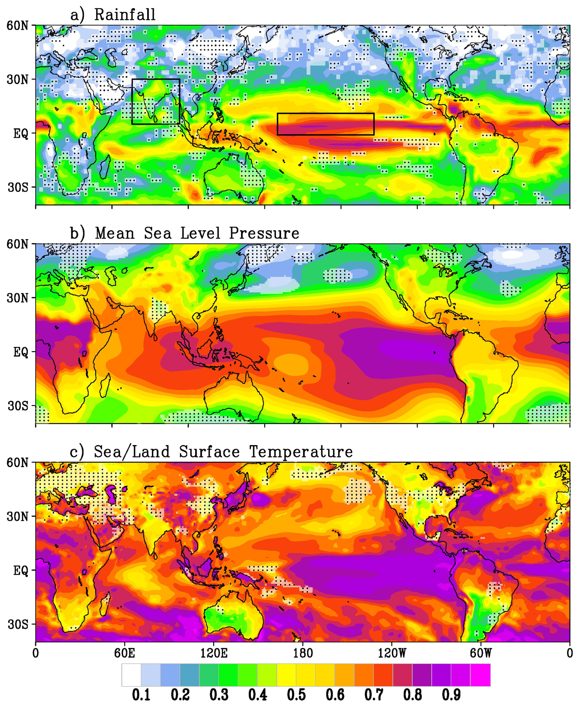
Figure 1 Potential predictability (shading) based on ANOVA method using equation no. 5. for JJAS averaged (a) rainfall, (b) mean Sea level pressure, (c) Sea/land surface temperature using CFSv2 re-forecast of 41 years (1981–2021) and 52 ensemble members. Signal-to-noise paradox regions (where model correlation skill with observations is higher than the potential predictability) are stippled with black dots. White semi-transparent regions, mostly coinciding with stippled regions, represent RPC>1.0.

Existing studies suggest that the SNP predominantly arises in the context of seasonal forecasting, which encompasses timescales of a month and beyond, as opposed to weather or medium-range predictions. This distinction can be attributed to the fundamental nature of weather forecasting, characterized as an initial value problem, where precision in the initial conditions takes precedence. Conversely, when dealing with forecasts spanning from seasonal to decadal and even longer timescales, slowly evolving boundary conditions (e.g., SST, soil moisture) and external forcings (e.g., solar variability, volcanic eruptions) become more prominent. These factors are the sources of predictability of the second kind. As the forecast lead time increases, the influence of initial errors wanes. In essence, in the realm of climate prediction, forecasts made several months or decades ahead depend significantly on the accurate representation of external drivers (e.g., greenhouse gas concentrations, aerosol emissions), the model's dynamics, its underlying physics, and the feedback mechanisms that operate within the model (i.e., internal variability). It is worth noting that the methodology employed in this study, namely ANOVA, is based on the framework of the “perfect model” paradigm. Here, the model is considered perfect or flawless, and any deviations in model simulations are attributed solely to errors in the initial conditions. This principle becomes particularly evident in large ensemble simulations, where even slight differences in initial conditions result in divergent model outcomes.

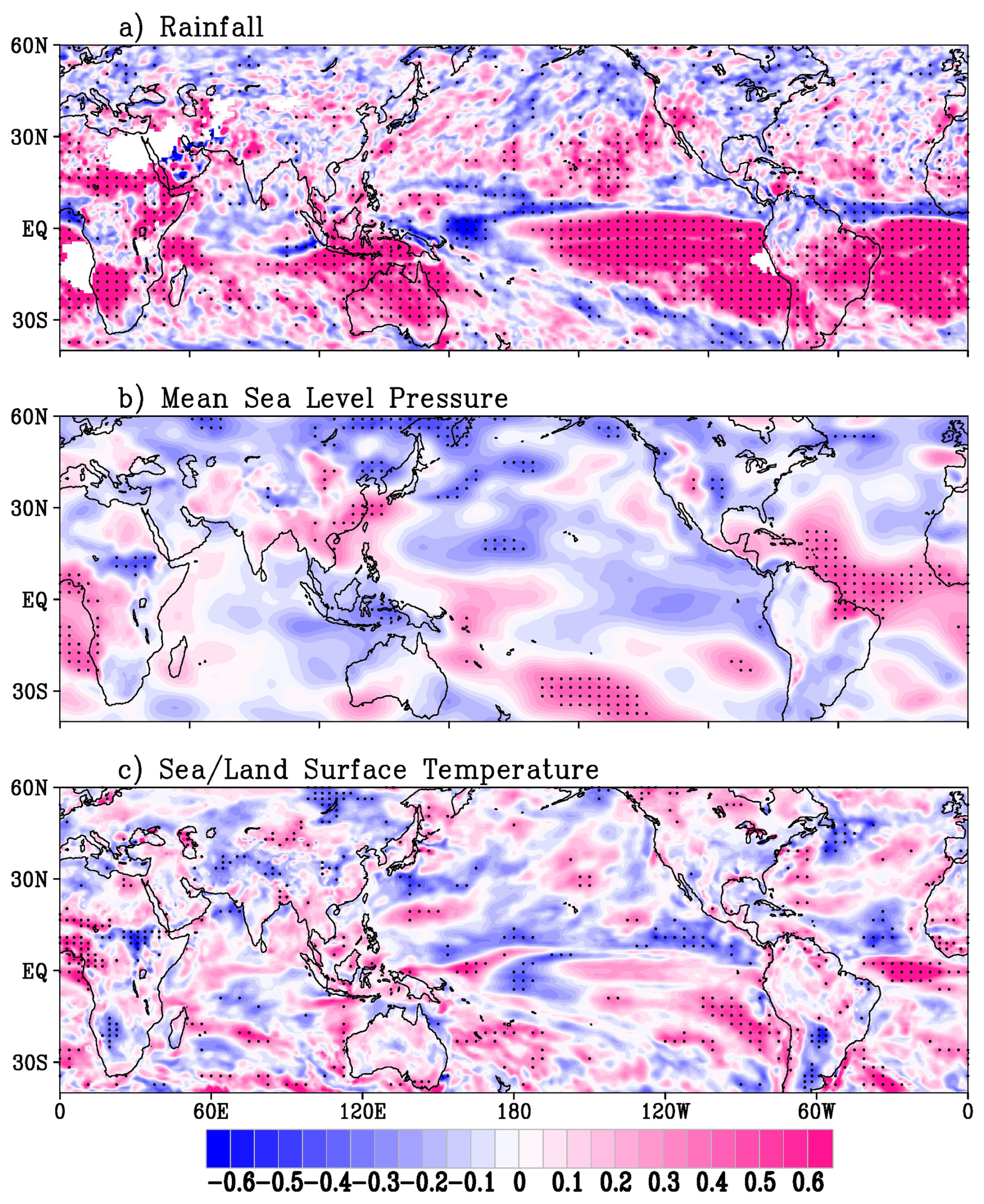
Figure 2 Test of orthogonality between signal and noise components. Correlations between signal and noise components of JJAS averaged (a) rainfall, (b) mean Sea level pressure, (c) Sea/land surface temperature employing CFSv2 re-forecast of 41 years (1981–2021) and 52 ensemble members. Correlations significant at 95 % (Student's two-tailed t test) and above are stippled by black dots.

As estimates of PPL and RPC depend on the signal-to-noise ratio (Sect. 2.3), the time series of the seasonal mean is partitioned into signal and noise components. Under the perfect-model assumption and within the ANOVA framework, the signal and noise components are expected to be clearly separated, that is, statistically independent of each other. Given that signal and noise inherently exhibit orthogonality, we examine the correlation between these components, aiming to ascertain the robustness of their partitioning. For rainfall, a substantial region in the tropics and sub-tropics exhibits statistically significant correlations between signal and noise components (Fig. 2). Conversely, in the case of MSLP and SST/LST, the significant area is smaller but extends across tropical and sub-tropical regions. Weisheimer et al. (2018) hypothesized that paradox emerges due to statistical problems in estimating RPC. Bröcker et al. (2023) also shows that signal and noise are not orthogonal in time, further undermining the assumptions underlying standard RPC estimation. Importantly, it should be noted that the regions displaying the paradox do not necessarily align with those demonstrating high or significant correlations between signal and noise. The paradox also persists in alternative measures used to estimate the PPL that do not explicitly rely on signal and noise variability (Scaife and Smith, 2018). Hence, it is plausible that precise partitioning into signal and noise components alone may not be sufficient to eliminate paradoxical behavior and, consequently, determine the true limit of potential predictability.

3.2 Signal-to-noise paradox in relation to model skill

As the name suggests, PPL is the maximum achievable skill by a model. However, its estimate does not have any binding relationship with the observations (i.e. observations are not required to estimate PPL). Nevertheless, it is important to understand how strong is the association between actual skill and estimated PPL. ENSO, as the dominant mode of global climate variability and a primary driver of both the ISMR and tropical Pacific variability, provides a fundamental source of seasonal predictability in these regions. Therefore it is logical to investigate whether and to what extent the model's actual skill aligns with the estimated potential predictability by examining the predictability of the Niño3.4 index along with regional precipitation in both paradoxical and non-paradoxical areas. Here we use time series data involving a predictor (Niño3.4 SST) and rainfall within two delineated regions (as shown in Fig. 1): one situated in the paradoxical region, denoted as the Indian Summer Monsoon Region (ISMR), and the other in a non-paradoxical region, referred to as the Pacific Region (PACR). These two contrasting regions are selected to investigate whether there are distinct variations in PPL with actual skill.

Furthermore, to test the association between PPL and actual skill, the ensemble members are arranged in ascending order in their absolute error in seasonal anomaly (with respect to GPCP data) for each year (i.e. ensemble members are arranged in a good-to-poor correlation skill order). We calculate predictability measures and correlations over a 21-ensemble member running window to see the general pattern. In the case of ISMR, although the PPL slightly decreases with diminishing skill, good ensemble members exhibit paradoxical behavior while poor ensemble members do not (Fig. 3). However, RPC varies with actual skill, as it is inherently a function of the correlation between model predictions and observations. For Niño3.4 and PACR, PPL does not fluctuate with actual skill, and the actual skill consistently remains significantly lower than the PPL. This implies that PPL is not contingent on a model's predictive skill. In other words, a higher PPL does not necessarily indicate that a model has the potential to achieve greater skill, which contradicts the objective of estimating PPL. Ensemble members are arranged from best to worst (or good to poor) to clearly show the relationship between actual skill and PPL.

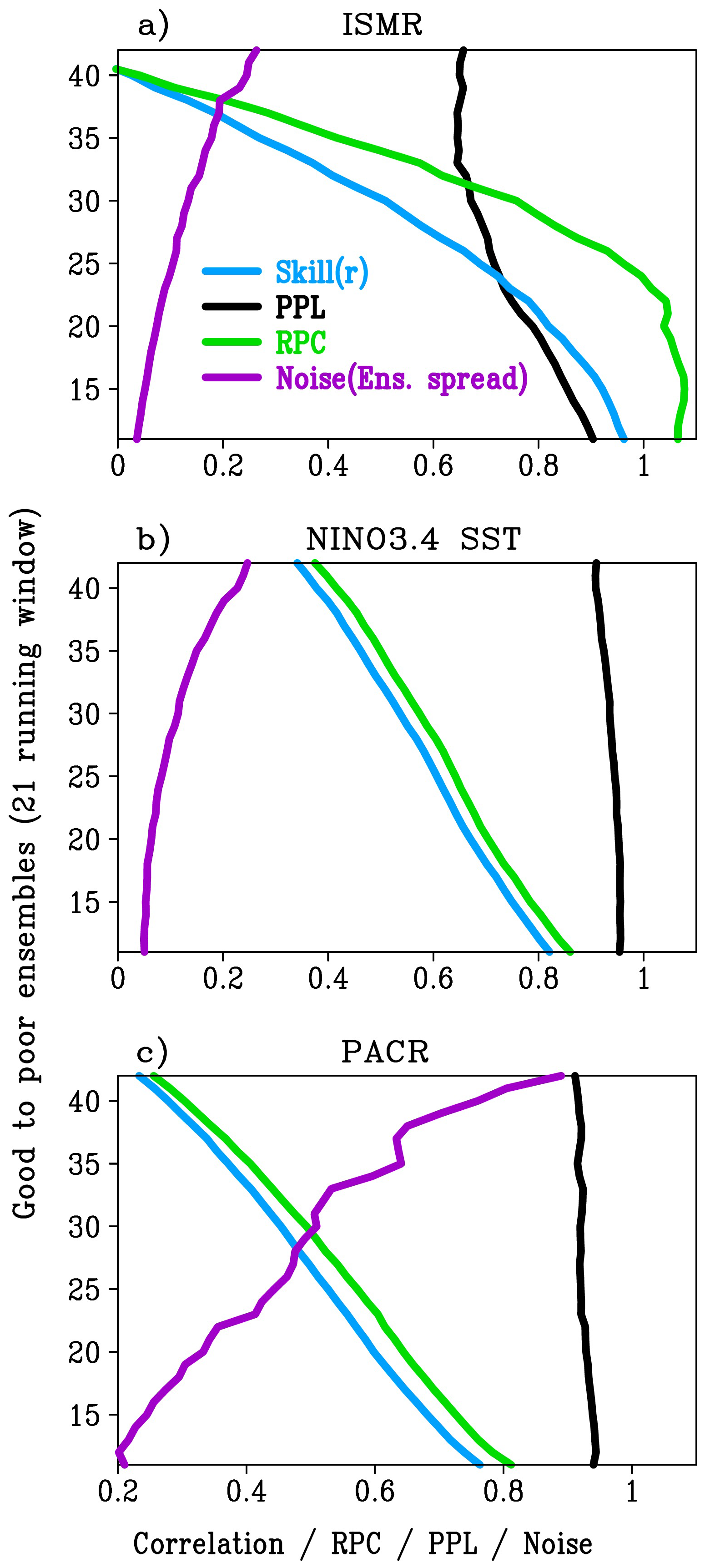
Figure 3 Correlation skill (blue), ANOVA based Potential predictability limit (PPL; black), Ratio of Predictable Component (RPC; green) and ensemble spread/“noise” component (purple) of arranged ensembles from good to poor and using a 21-ensemble moving window for (a) ISMR rainfall, (b) Niño3.4 SST, (c) PACR rainfall. Correlation skill is defined as the correlation between the ensemble-mean re-forecast and observations. The Niño3.4 index is used as a reference predictor to provide a baseline for ENSO-driven predictability of regional precipitation, allowing comparison with the model's full dynamical skill.

The estimated PPLs clearly do not represent the upper limit of seasonal prediction skill, raising the question of why such a discrepancy exists. A plausible explanation is that partitioning of seasonal mean into signal and noise components is problematic. It assumes, perhaps unrealistically, that the inter-ensemble spread in a year is only due to initial errors (see Sect. 2.3). Subsequently, we compute correlations between signal and noise components using a 21-ensemble moving window of arranged ensembles (Fig. 4). Remarkably, the results reveal a distinct pattern where correlations strengthen and become statistically significant for ensemble members exhibiting greater bias in the seasonal anomaly. While the correlation between signal and noise becomes stronger (inverse correlation) as we move from good to poor ensembles (Fig. 3), particularly for PACR, the PPL remains relatively constant (Fig. 3c). We also note that for the ISMR, even though the paradox persists in the case of good ensemble members (as shown in Fig. 3a), the correlation between the signal and noise components is relatively stronger for good (r=0.2) and poor ($r=-\mathrm{0.2}$) ensemble members (Fig. 4). Therefore, above all suggest that accurate partitioning into signal and noise components is also not a sufficient criterion for obtaining the true estimates of PPL. This is consistent with the findings of Scaife and Smith (2018), who showed that paradoxes can arise even in PPL estimates that do not explicitly rely on the separation of signal and noise components.

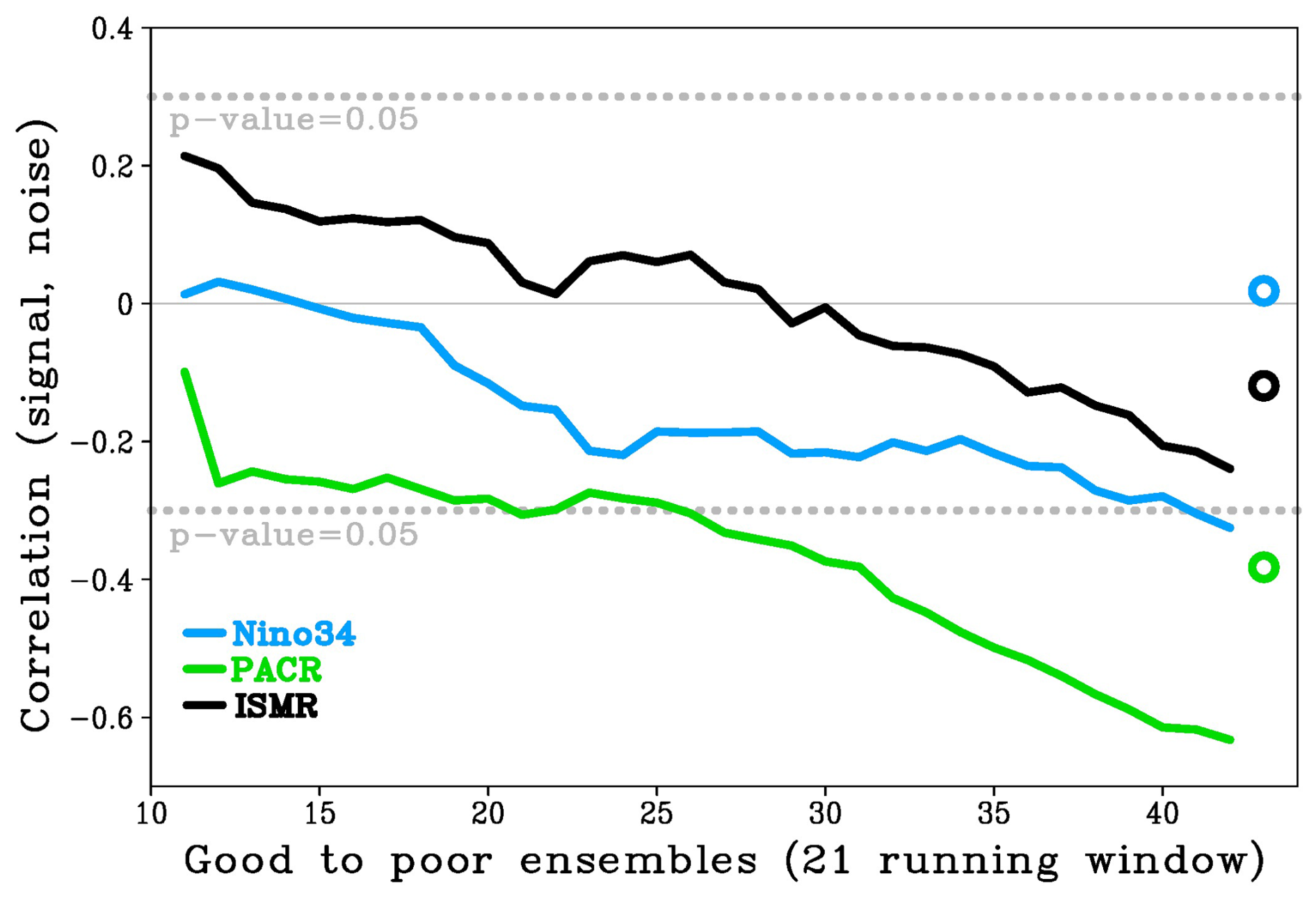
Figure 4 Correlations between signal and noise components estimated based on the ANOVA method. Correlations using all 52 ensemble members (open circles) and a 21-ensemble member moving window, where ensemble members are arranged from good to increasingly poor ensembles, are shown for ISMR (black), PACR (green), and Niño3.4 SST (blue). The grey dotted line indicates correlations that are significant at the 95 % confidence level.

Apart from PPL, it is also important to assess how skillful the model is in predicting both the predictors and the predictands. Given two contrasting regions for analysis of predictands (i.e. ISMR, PACR), we have evaluated the prediction skill for these predictands and major global predictors – i.e. Niño3.4 index, Indian Ocean Dipole (IOD), Pacific Decadal Oscillation (PDO), and Atlantic Multi-decadal Oscillation (AMO). It is noteworthy that a diverse range of correlation skills is evident among ensemble members (Fig. 5). However, it is important to underscore that the skill exhibited by the ensemble mean (indicated by the red circle) consistently surpasses that of the average of the individual members (depicted by the blue circle). Furthermore, aside from the IOD, the correlation skill for all other predictors and both predictands remains statistically significant at or above the 99 % confidence level. This highlights the model's proficiency in forecasting both the predictors and predictands, which is essential for further analyzing their complex relationships with other components of the climate system, such as sub-seasonal components. However, the RMSE exceeds 100 % of the observed standard deviation (Fig. 5b), indicating that the model's errors are greater than the natural variability in the observed data.

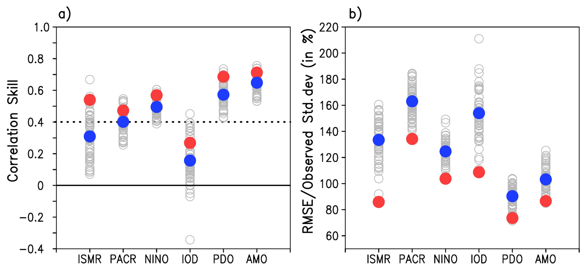
Figure 5 (a) Prediction skill (correlation) of major predictors (NINO → Niño3.4 index; IOD → Indian Ocean dipole index; PDO → Pacific Decadal Oscillation; AMO → Atlantic Multi-decadal Oscillation) and predictands (ISMR → Indian Summer Monsoon Rainfall averaged over the box shown in Fig. 1a; PACR → area-averaged rainfall over the Pacific box; Fig. 1a) in CFSv2 using 41 years of re-forecast (1981–2021) and observations. (b) RMSE compared to observed standard deviation (i.e. RMSE/Obs. Std.). Grey open (red solid) circles represent individual (averaged) ensemble member skills. The blue solid circle represents the average skill of individual members (i.e., the average of the grey circles). The black dashed line represents the significance level of correlation values at the 99 % confidence level.

3.3 Role of sub-seasonal components

Although the advent of computers in the 1950s gave hope for accurate weather prediction, Lorenz's work (Lorenz, 1963) revealed the inherent unpredictability beyond a few days due to non-linearity in the systems. Subsequently, Charney and Shukla (1981) pioneered the concept of long-lead predictability in the tropics (e.g. monthly/seasonal mean) due to the influence of slowly varying boundary conditions (e.g., SST, soil moisture) on atmospheric instabilities. Recent studies have shown that sub-seasonal components of the Indian summer monsoon, in association with global predictors (e.g., ENSO, AMO, etc.), significantly contribute to the inter-annual variability of the ISMR (Saha et al., 2019, 2020, 2021). The sub-seasonal components are the building blocks of the seasonal mean. Moreover, precipitation is a discrete phenomenon that comes as an event (either zero or a positive value). The annual/seasonal cycles of precipitation are composed of these discrete events. The sum of these events constitutes the seasonal, or annual mean. In principle, for any predictor affecting a predictand, the predictor communicates through the modulation of sub-seasonal components, which are then projected onto the seasonal/decadal anomaly of the predictand. However, due to the inherent non-linear characteristics of sub-seasonal components, it is plausible that their variability may not be entirely predictable. In such cases, a portion of the sub-seasonal variability may remain associated with relevant predictors, contributing to overall seasonal predictability (illustrated through schematic in Fig. 6). Given that sub-seasonal components constitute fundamental elements of seasonal rainfall, the seasonal prediction skill can be assessed through an examination of the co-variances between sub-seasonal components and seasonal rainfall/predictors (see Sect. 2.3.3, Eqs. 7–12). Moreover, the co-variance of sub-seasonal components with seasonal rainfall, in relation to PPL and ensemble spread, can likely be attributed to imperfect physics and can be demonstrated. To further elucidate this relationship, we have organized ensemble members in ascending order from more accurate to less accurate, i.e., from good to poor ensembles, based on seasonal rainfall anomaly (ISMR and PACR) compared to observations (i.e. GPCP rainfall).

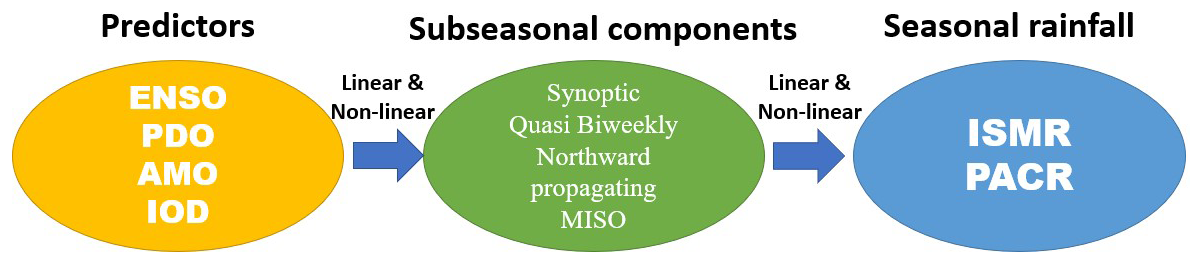
Figure 6 A schematic diagram illustrates how slowly varying predictors influence seasonal rainfall anomaly by modulating sub-seasonal components. The sub-seasonal components are considered the building blocks of seasonal rainfall. Highlighting the dominant role of sub-seasonal variability in modulating seasonal monsoon precipitation (specific to tropical/monsoon regions).

The sub-seasonal variances are computed within three distinct bands: 2–5 d (synoptic), 10–20 d (bi-weekly/super-synoptic), and 20–60 d (MISO, MJO). If sub-seasonal components indeed play a role in the prediction skill of seasonal rainfall, their co-variability should exhibit distinguishable patterns among good and poor ensembles. As global daily gridded rainfall observation data (GPCP) is available from October 1997 onward, our analysis is conducted for the period spanning from 1997 to 2021. It is worth noting that similar paradoxical behavior is evident in the model during this time frame, as depicted in Fig. S4. It is evident that the co-variance across these three bands gradually increases from good to poor ensembles in both the ISM and PAC regions (Fig. 7a and b). Notably, for the ISM region, the 2–5 d variability exhibits a distinct contribution to seasonal prediction skill from good to bad ensembles, whereas contributions of the 10–20 and 20–60 d bands are more significant for predicting the seasonal anomalies in the PAC region. Moreover, the model exhibits a considerable spread in the co-variances, particularly in the lower frequency bands (Fig. 7c and d). These distributions of co-variances are also skewed in relation to the observations, a phenomenon that carries clear implications for model prediction skill. We also observe that the noise or ensemble spread increases (Fig. 3) as the error in the co-variance grows from good to poor ensemble members (Fig. 7a and b).

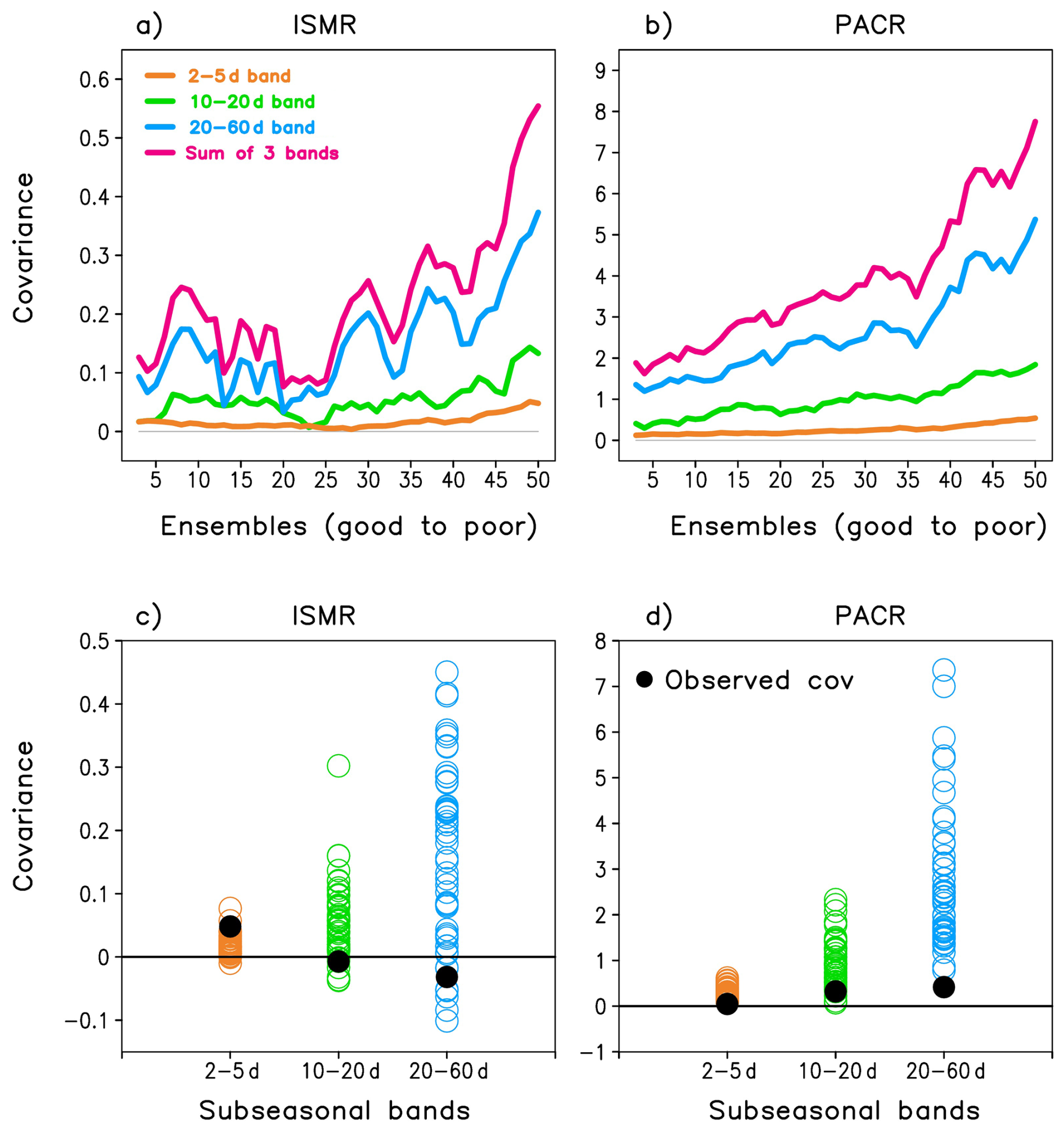
Figure 7 Inter-annual co-variance between sub-seasonal variances in three bands (2–5, 10–20, 20–60 d) and mean rainfall in the ISM and PAC domains (1997–2021). Line plots of co-variances arranged from good-to-poor ensemble members (compared to observed seasonal anomalies) in a 5-ensemble moving average window for (a) the Indian summer monsoon domain and (b) the Pacific domain. Co-variances in each ensemble member at three sub-seasonal bands, along with observations for (c) ISMR and (d) PACR.

It may be noted that, in the case of seasonal prediction, the statistics of sub-seasonal components are important and not the actual timing of their occurrence. Moreover, the simulation of sub-seasonal statistics depends on the physics, dynamics, and their coupling with various components of the Earth's climate system (e.g., land, ocean, atmosphere). In general, global coupled models have serious difficulties in simulating synoptic systems, such as lows and depressions. Nevertheless, these synoptic events contribute significantly to the mean and variability of seasonal climate (e.g. Yoon and Chen, 2005; Saha et al., 2019). A disproportional contribution of sub-seasonal components to the seasonal mean is a big concern, as it can spoil the prediction skill, which is evident in Fig. 7.

It is now evident that the model's ability to simulate the sub-seasonal contribution to seasonal anomalies significantly influences seasonal prediction skill. In addition to co-variability, it is equally important that the model accurately replicates the mean sub-seasonal components with high fidelity. Figure 8 provides an overview of the mean sub-seasonal variances within three temporal bands, both in absolute terms and as a percentage of the total variance. The model consistently underestimates synoptic (2–5 d band) variance in both the ISM and PAC regions. In the PAC region, both the 10–20 and 20–60 d band variances are overestimated. When considering the total variance, the model overestimates it in both regions. Although the paradox has been shown to be most pronounced when the model's total variance closely matches that of observations (e.g., Scaife and Smith, 2018), the model used here exhibits higher total variance than observed over the South Asian monsoon region (Sect. 3.2; Figs. 5b and 88c, d). This suggests that over-dispersion may contribute to the low signal-to-noise ratios diagnosed. Nevertheless, the persistence of paradoxical behavior even under these conditions underscores the influence of other model imperfections, including biases in sub-seasonal variability, in limiting predictability. Moreover, when expressed as a fraction of total variance, the synoptic-band variance is severely underestimated, accounting for only 2 %–7 % of the total variance (Fig. 8a and b) across ensemble members. It is intriguing to observe that in the observations, the synoptic variance contributes approximately 15 % and 26 % to the total variance over the ISM and PAC regions, respectively. The 20–60 d band is overestimated in the PAC region while slightly underestimated in the ISM region. Consequently, a discernible systematic trade-off emerges between the synoptic and MISO/MJO contributions within the model. This trade-off likely plays a role in explaining the model's comparatively lower prediction skill.

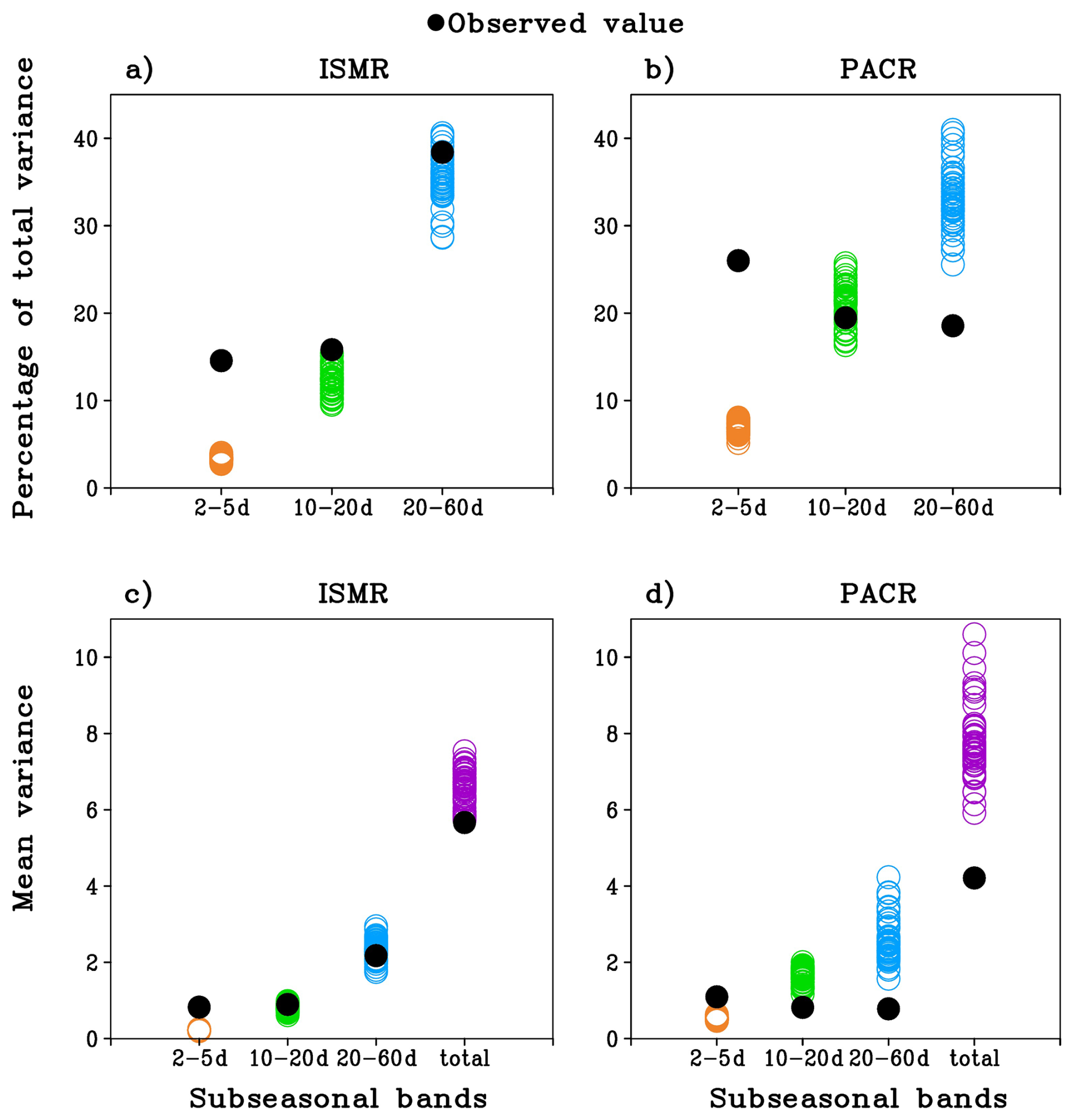
Figure 8 Mean sub-seasonal rainfall variances simulated by the model and observations (1997–2021). Variances in the 2–5, 10–20, and 20–60 d bands with respect to the total variance (in %) over (a) the ISM domain and (b) the Pacific domain. (c) and (d) are the same as a) and b), respectively, but show their actual values.

Using multiple correlation analysis, we further investigate the impact of major global predictors, including ENSO, AMO, IOD, and PDO, on sub-seasonal components. Our analysis reveals significant patterns of association between these predictors and sub-seasonal bands (see Fig. 9), reaffirming the findings of Saha et al. (2021). Observations show that, in the ISM region, the synoptic bands have the strongest association with these predictors. However, the 10–20 and 20–60 d bands in the PAC region demonstrate more pronounced connections with the predictors. As expected, the model shows a wide range of associations between sub-seasonal components and predictors. A notable deviation is observed in the PAC region, where 2–5 d band and 20–60 d bands overestimate their associations with the predictors. Analogous to the patterns observed in Fig. 7a and b, the multiple correlation distinctly separates good and poor ensemble members for PACR rainfall (Fig. S5). However, for the ISMR, this distinction is not very prominent. Nonetheless, this analysis underscores the significance of major global predictors influencing sub-seasonal components, thereby elucidating the intricate dynamics that exert an influence on seasonal prediction skills.

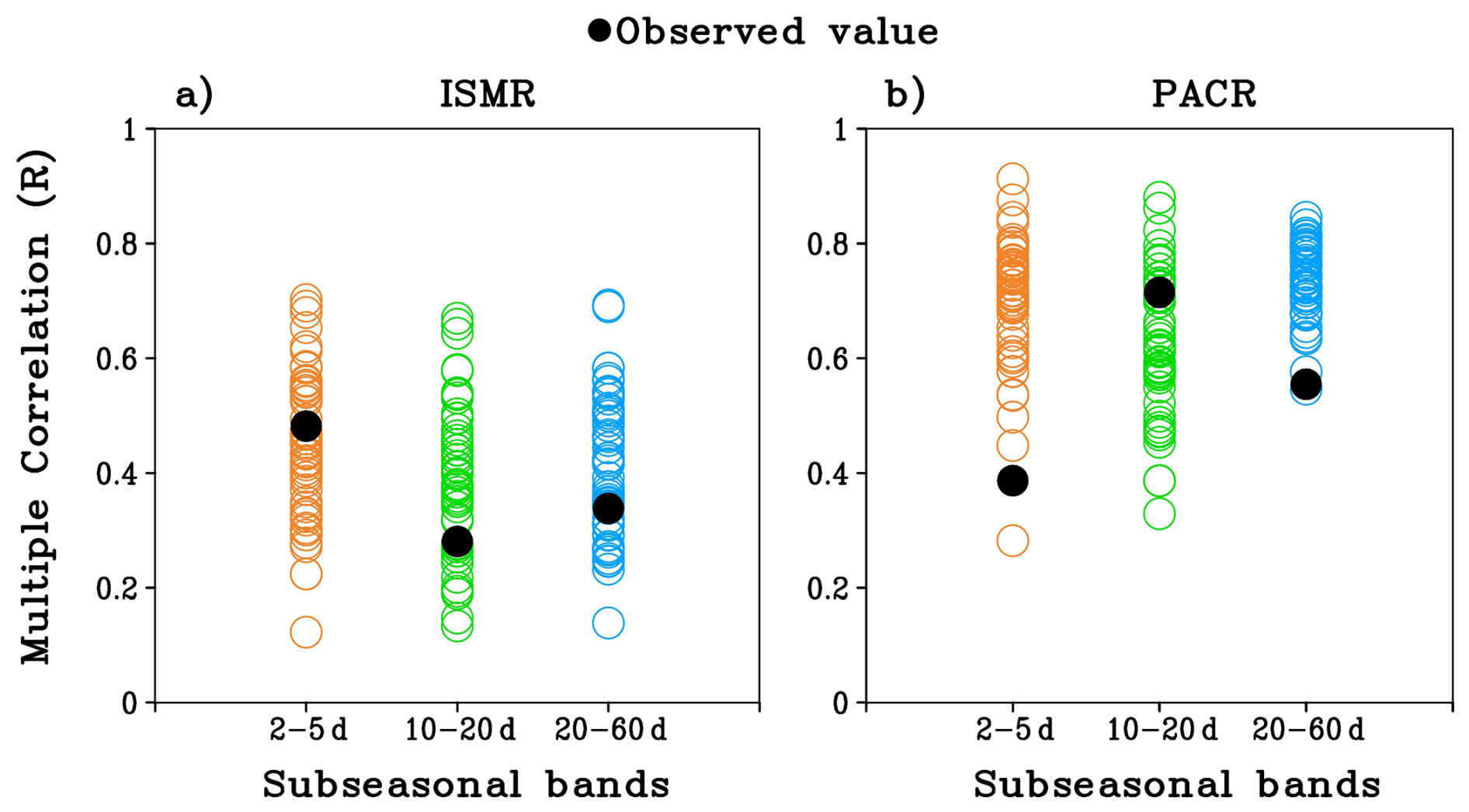
Figure 9 Multiple correlation analysis of sub-seasonal components (three bands) regressed with four global predictors (Niño3.4, IOD, PDO, AMO) for (a) ISMR and (b) PACR rainfall. Open circles represent individual ensemble members of the model, and black solid circles represent those in the observations.

Therefore, a significant association of sub-seasonal rainfall variance with the seasonal mean rainfall and four major global predictors is found in observations and, to a varying degree, in model simulations. Conversely, the model's shortcomings in capturing interactions between fast (i.e. sub-seasonal) and slowly evolving components (e.g. ENSO) influence the seasonal mean and its variability. Consequently, the feasibility of estimating the PPL based on the “perfect model” framework (or ANOVA) appears inadequate. The paradox we identify is therefore an expected consequence of the perfect-model assumption itself, which neglects real model errors and biases in sub-seasonal variability. We recall that the “perfect model” framework assumes that the ensemble spread is due to an error in the initial conditions, and error growth due to imperfect physics or numerical scheme is not considered. It is crucial to acknowledge that real-world models are imperfect, and the realization of a truly perfect model is highly unlikely. Hence, the question arises: How can we obtain a reliable estimate of PPL that circumvents paradoxical behaviour?

4 Summary and discussions

In this study, we employ a data set comprising 52 ensemble member re-forecasts spanning a 41-year period from 1981 to 2021, as simulated by the IITM CFS (Saha et al., 2019). The primary objective of this study is to elucidate the underlying factors contributing to the signal-to-noise paradox in seasonal climate prediction within the tropical and subtropical regions. We observe that many regions exhibit a signal-to-noise paradox when estimated by subtracting correlation skill from potential predictability estimated by the ANOVA method (Fig. 1). This region also corresponds to areas where the ratio of predictable component (RPC) exceeds one. Several prior studies have highlighted the presence of paradoxes in PPL estimates within the “perfect model” framework (i.e. ANOVA). However, the underlying causes remain a subject of ongoing debate within the scientific community. As paradoxical behavior is rare in weather time scale but prevalent on seasonal to decadal and beyond time scale, assessment of the underlying hypothesis for the method of estimating PPL is warranted. Therefore, to delve deeper into the intricacies of this paradoxical behavior, we examine rainfall patterns in two distinct tropical regions: the Indian summer monsoon region (ISMR), exhibiting paradoxical behavior over half of the region, and the central Pacific region (PACR), without any paradox.

While correlation skill in the time series of seasonal ISMR and PACR rainfall decreases from relatively good to poor ensemble members (arranged with respect to observations), the PPL exhibits minimal variation (Fig. 3). This suggests that PPL is not closely associated with the actual skill of a model, contradicting the fundamental purpose of estimating it. In the ANOVA method, the separation of a forecast into “signal” and “noise” components is based on the assumption that initial error gives rise to the “noise”, while the model is considered to be perfect. Consequently, there should be no temporal relationship between “noise” and “signal” components. Conversely, it is observed that a significant and robust correlation exists between these components. Furthermore, regions exhibiting paradoxical behavior do not necessarily coincide with areas of significant correlation between the “signal” and “noise” (Fig. 2).

Hence, the central issue underlying this problem is why the ANOVA method falls short in estimating climate predictability? What leads to the apparent inadequacy in separating a forecast into “signal” and “noise” components? Some of the answers can be found in the nature of the problem. Weather forecasting pertains to the predictability of the first kind, where the accuracy of initial conditions plays a primary role, and slowly evolving boundary conditions play a secondary role. Conversely, seasonal/decadal forecasting is categorized as predictability of the second kind, where slowly evolving boundary conditions play a major role. Moreover, the physical processes which affect the sub-seasonal variability at various frequencies (e.g. lows and depressions, MJOs, etc.) can also affect the seasonal mean. As the real world’s models are not perfect, these deficiencies can also add to the variability or ensemble spread in addition to that due to errors in the initial conditions.

Therefore, understanding the co-variability between sub-seasonal components and seasonal means within the context of predictability and prediction is of paramount importance. While prediction skill demonstrates systematic variations with the covariance between sub-seasonal components and seasonal mean rainfall, the PPL remains quite invariant (Fig. 3). It becomes evident that the model exhibits a broad and often skewed range of co-variability between sub-seasonal variance and seasonal mean in comparison to observations, with sub-seasonal components strongly linked to global predictors (see Figs. 7 and 9). Additionally, ensemble spread (or noise component) is found to vary systematically with this co-variance and prediction skill (Figs. 3 and 7). Consequently, a robust methodology for estimating PPL must consider not only the errors in initial conditions but also those arising from model physics, dynamics, and numerical methods employed. These findings underscore the critical significance of accurately simulating sub-seasonal components and their co-variability in seasonal prediction, shedding light on factors influencing prediction skill and identifying potential areas for model enhancement.

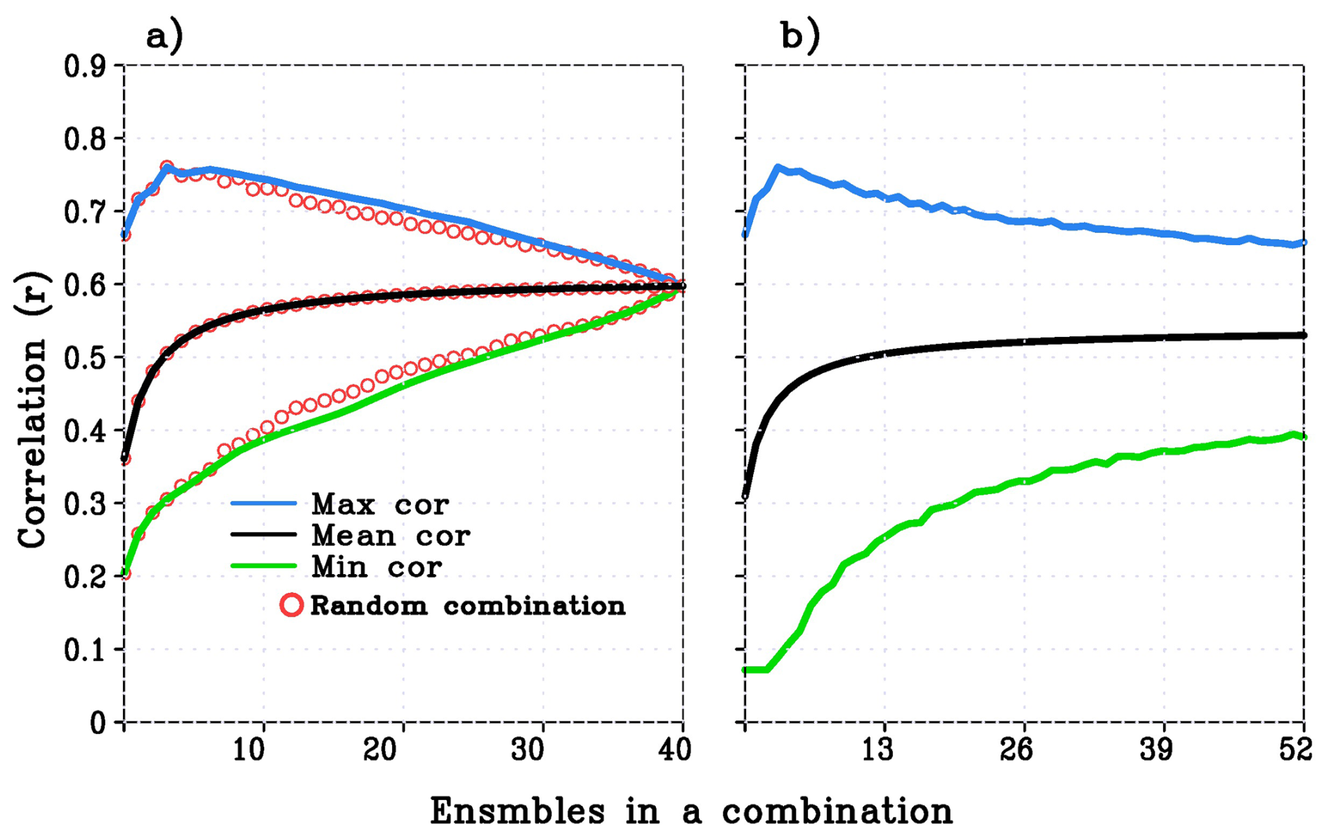
Figure 10 (a) The maximum (blue solid line), mean (black solid line), and minimum (green solid line) correlation skill using all combinations of n ensemble-averaged ISMR rainfall (i.e., ⁴⁰C_n, where n varies from 1 to 40). Similarly, the red open circles show the correlation skill using 1 million random combinations of n ensemble-averaged ISMR rainfall. (b) The maximum (blue solid line), mean (black solid line), and minimum (green solid line) correlation skill using the Bootstrapping method with 10 million random combinations of n member ensemble-averaged (n varies from 1 to 52).

Even when using the same forecasting model, different realizations of initial conditions (ICs) can produce forecasts with varying levels of skill. While predictability refers to the intrinsic potential of the climate system, the PPL represents the maximum achievable skill of a specific forecast system. Within a fixed modeling and data assimilation framework, variations in prediction skill arise from differences in IC realizations. Moreover, estimating this maximum achievable skill, or PPL, ideally requires a very large number of ensemble simulations, which is computationally expensive. To address this limitation, random subset sampling and bootstrapping techniques may provide efficient and statistically robust alternatives (e.g., Saha et al., 2019). Using the best 40 out of 52 ensemble members, the maximum, minimum, and mean prediction skills were evaluated as correlations between observations and ensemble means across all possible combinations (i.e., ⁿC_r, where n is the total number of ensembles and r is the subset size; Fig. 10a). The results show that subsets of approximately 5–10 ensemble members yield a maximum correlation skill of about 0.76, representing the maximum achievable skill and thus a plausible estimate of the model's PPL. It is theoretically possible that a balanced distribution of positive and negative skill among ensemble members could produce a high maximum attainable skill while the ensemble-mean skill remains insignificant. In the present analysis, however, both the maximum and minimum attainable skills remain positive, indicating that a high maximum skill cannot occur when the realized prediction skill is near zero.

However, the use of large ensemble sizes imposes substantial computational demands. For example, with 52 ensemble members, there are approximately 4.9×10¹⁴ possible subsets of 26 members (without repetition), making exhaustive evaluation impractical. As an alternative, a limited number of randomly selected subsets (up to one million) could be generated without repetition of ensemble members. Notably, similar patterns of maximum, minimum, and mean correlations emerge when compared with the full combination space (red circle mark in Fig. 10a). Furthermore, the mean, minimum, and maximum correlations tend to converge as the number of combinations increases, demonstrating that random subset sampling provides a computationally efficient and reliable approach without compromising the robustness of the results.

Using bootstrapping, this framework can be further extended by allowing repetition of ensemble members within subsets, thereby enabling the generation of millions of synthetic ensemble combinations from a limited dataset (Fig. 10b). This resampling strategy effectively increases the sample size and improves the reliability of population-level statistics, particularly for estimating extremes such as the maximum attainable forecast skill. Consequently, it provides a robust estimate of the achievable performance range of the forecasting system. Importantly, this methodology can also be extended to grid-point-level analysis for the same three variables (rainfall, MSLP, and SST/LST), enabling the construction of spatial maps of maximum achievable skill (Fig. S6). We further note that the spatial pattern of maximum skill shows the highest values over the tropical Pacific region compared to other parts of the globe, consistent with earlier findings (e.g., Shukla, 1998).

This approach enables diagnostic quantification of the range of prediction skill attainable by the model when evaluated against observations. However, estimates of maximum skill should be interpreted cautiously, as they may be affected by sampling uncertainty associated with finite ensemble size. We emphasize that this framework is intended as a diagnostic sensitivity analysis rather than an operational forecasting methodology. In real-time prediction systems, the growth of initial condition errors, together with model errors, limits the practical attainability of the predictability limit, and the a priori identification of “best” ensemble members is not feasible. Nevertheless, emerging AI–ML approaches, trained on longer model simulations, reanalyses, and observational datasets, offer a potentially promising pathway by learning complex subseasonal-to-seasonal relationships with large-scale predictors (e.g., Sharma et al., 2025), which may help mitigate error growth and enhance operational monsoon forecasting skill with longer lead time in the future.