The Atlantic ocean's decadal variability in mid-Holocene simulations using Shannon's entropy

Quantifying climate variability in a way that is comparable across models, experiments, and observations remains challenging, particularly at decadal time scales where nonlinear dynamics dominate. Traditional variance-based metrics are sensitive to anomaly amplitude, mean-state biases, and units of measurement, limiting their robustness for inter-model analyses. Here, we introduce an information-theoretic framework that characterizes climate variability as trajectories in a discrete phase space and quantifies system organization using Shannon’s entropy. Using four coupled models (EC-Earth, GISS, iCESM, and CCSM-Toronto), we apply our methodology to compare the models' tropical and South Atlantic decadal variability, analyzing their sea surface temperature (SST) and precipitation under Pre-Industrial and mid-Holocene boundary conditions, including Green Sahara experiments, and compare the results with observational datasets. Mid-Holocene forcings lead to model-dependent entropy changes, indicating a reorganization of Atlantic decadal variability rather than a uniform response across models. Green Sahara boundary conditions reduced SST entropy in EC-Earth and GISS models, implying a more organized Atlantic system, while precipitation responses are more heterogeneous. Entropy values derived from principal-component-based phase spaces have shown a more consistent framework to compare numerical models varaibility with observational estimates than using the traditional regional SST boxes index-based phase space. These findings highlight the diverse representations of climate variability across models. As such, this framework enables robust comparisons of low-frequency climate variability across models, paleoclimate simulations, and observations, complementing traditional variance-based diagnostics.

1 Introduction

A system's variability can be perceived as the absence of uniformity across multi-scales (Sang, 2013). Earth's climate can be interpreted as a high-dimensional chaotic system (highly dependent on initial conditions), and understanding the structure and drivers of climate variability remains a central challenge in climate science, particularly at decadal time scales where internal dynamics and external forcings interact in nonlinear ways. (Ghil and Lucarini, 2020; Kwiecien et al., 2022). Traditional approaches to characterizing variability often rely on variance-based metrics or spectral analyses, which are sensitive to amplitude, mean-state biases, and the choice of variables or units (Ghil et al., 2002; Froyland et al., 2021). While these methods have been important in identifying dominant modes of variability, they provide limited insight into how climate systems explore their range of possible states, how persistent those states are, and how transitions between them evolve under different climate forcings (Sane et al., 2024). The tropical and South Atlantic Ocean (15° N–30° S, 60° W–20° E, region defined in the maps “a” and “b” from Fig. 1) play a fundamental role in regulating global climate through their influence on the interhemispheric energy balance, the position of the Intertropical Convergence Zone, and the coupling between sea surface temperature (SST) and precipitation (Dhrubajyoti et al., 2019; Hounsou-Gbo et al., 2019; Atwood et al., 2020). Decadal variability in this region is associated with large-scale Atlantic modes that modulate rainfall over South America and Africa and interact with both extratropical and tropical circulation patterns (Gorenstein et al., 2023). Because these modes arise from coupled ocean–atmosphere processes, changes in their organization or persistence can have far-reaching climatic impacts (Deser et al., 2010), while underscoring the difficulty in predicting their evolution due to their reliance on a wide range of interacting climate variables (Deser et al., 2012).

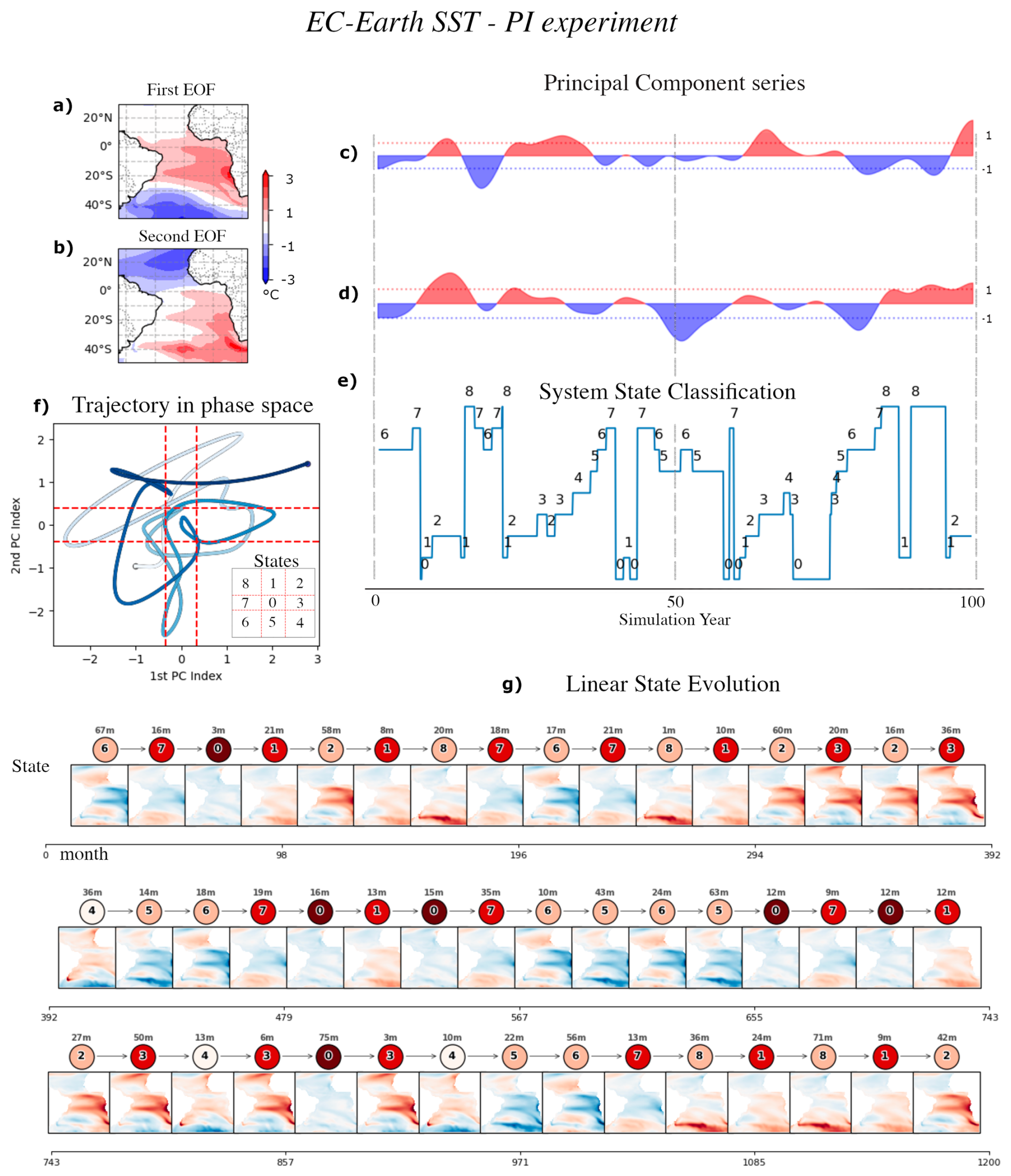
Figure 1 EC-Earth SST system state identification and evolution during the PI experiment. (a) The first EOF; (b) The second EOF; (c, d): their respective PC series, blue for negative and red for positive, dashed lines indicating the 1 standard deviation value. (e) The cluster identification of the discrete system state, given by the two PC indices above. (f) The system's trajectory in the continuous PC phase space. The line's color represents the time evolution, white for the start (month 0) and dark blue for its end (month 1200). (g) The diagram illustrates the state-by-state evolution of the system over time. Each node represents a specific SST pattern, identified by its cluster number (referenced in panels e and f) and its spatial pattern displayed below the node. The numeral positioned above each node indicates the duration, in months, that the system remained in that state before transitioning. Darker shading on a node signifies a higher frequency of transitions into that specific cluster throughout the entire time series.

The mid-Holocene (MH) period, approximately 5000–7000 years Before Present, provides a natural framework to investigate how external forcings reshape climate variability. Orbital changes during this period altered the seasonal and latitudinal distribution of insolation, leading to profound hydroclimatic changes (Berger, 1988; Liu et al., 2002; Bova et al., 2021), most notably the African Humid Period and the expansion of vegetation over the Sahara (Demenocal et al., 2000). Proxy studies and climate model simulations suggest that these boundary-condition changes affected not only mean climate states but also the dynamics of tropical and Atlantic variability through land–atmosphere–ocean feedbacks (Pausata et al., 2016; Smith and Mayle, 2017; Gorenstein et al., 2022a). Rather than simply amplifying or damping anomalies, quantifying how such forcings reorganize decadal variability remains an open problem, particularly when comparing across models with differing physics and parameterizations.

The geophysical mechanisms behind the Atlantic Ocean modes coupling with pressure and wind driving decadal precipitation anomalies were unraveled using observational data in Gorenstein et al. (2023). When examining the dynamics of this region in climate simulations, a more fundamental question arose regarding how to assess its decadal variability. Since numerical models present biased climate representations compared to observational data and among themselves (Dhrubajyoti et al., 2019), their climate variability is not typically measured in relation to large-scale climate patterns, such as ocean modes. This motivated us to create a new method using ocean modes and their precipitation counterparts to quantify decadal variability in numerical climate models.

In this study, we adopt an alternative perspective grounded in information theory to characterize climate variability as the evolution of a system through a discrete phase space. By representing SST and precipitation anomalies as trajectories in low-dimensional spaces and applying Shannon’s entropy to measure the organization of the Atlantic Ocean modes and their precipitation counterparts. This framework allows us to compare Pre-Industrial and mid-Holocene climate simulations across multiple models, as well as observational datasets, within a unified and scale-invariant metric. By doing so, we aim to assess how mid-Holocene forcings reshape the persistence and transitions of dominant Atlantic climate states, offering a complementary and physically interpretable measure of climate variability beyond traditional variance-based approaches.

2 Material and Methods

Simulations from four numerical climate models (EC-Earth, iCESM, CCSM-Toronto, and GISS) are used to study decadal climate variability of the tropical and South Atlantic (25° N–45° S, 60° W–20° E) Sea Surface Temperature (SST) and precipitation, as well as their sensitivity to prescribed parametrizations. The simulations are separated into pre-industrial boundary conditions (PI), simulations using mid-Holocene insolation boundary conditions (MH_PMIP), and simulations using mid-Holocene insolation and different vegetation inputs (MH_GS). Details defining each numerical simulation are described below. All the data used in this study is summarized in Table 1.

2.1 Data

2.1.1 EC-Earth

The European Consortium Earth System Model Version-3 (EC-Earth) scenarios analyzed in this study were: PI (100 years run B405 and 200 years run B400), MH_PMIP (100 years run Z6KA and 200 years run B6KA), MH_GS (100 years run G105 and 50 years run G100, simulations with prescribed vegetation in the Sahara region) and MH_GSdr (100-year run G506, and 200-year run G501, simulations with prescribed vegetation in the Sahara region and dust reduction).

EC-Earth standard configuration consists of the atmosphere model IFS, including the land surface module HTESSEL and the ocean model NEMO3.6 with the sea ice module LIM3. Coupling variables are communicated between the different component models via the OASIS3-MCT coupler (Döscher et al., 2022). The EC-Earth model is used to contribute to CMIP6 in several configurations, for example, the EC-Earth3-Veg configuration, which couples the LPJ-Guess dynamic vegetation model (Smith et al., 2014) to the atmosphere and ocean model. However, the performance of EC-Earth3 and EC-Earth3-Veg is very similar (Wyser et al., 2020).

2.1.2 CESM models

The Community Earth System Model (CESM) outputs from different scenarios used were from CCSM-Toronto: PI, MH_PMIP, MH_GS, and MH_GSsl (with prescribed soil and lake inputs), 100 years run each; and iCESM: PI, MH_PMIP, MH_GS (100 years run each).

The CESM models used here are from the CMIP6 multi-model ensemble. The CCSM-Toronto simulations are a PMIP experiment for the mid-Holocene with Green Sahara and mid-Holocene with soil and lake inputs made by the University of Toronto (UofT), Canada. The model configuration was made by UofT-CCSM4 (2014), atmosphere from CAM4 (finite-volume dynamical core; 288 × 192 longitude/latitude; 26 levels; top level 2 hPa) (Peltier and Vettoretti, 2014); ocean: POP2; sea ice: CICE4; land: CLM4. The iCESM simulations used in this study were first presented in Tabor et al. (2020). iCESM is configured with CAM5, POP2, CLM4, CICE4, and RTM (Brady et al., 2019; Hurrell et al., 2013). The atmosphere and land have a 1.9 × 2.5° horizontal resolution, and the ocean and sea ice have a nominal 1° horizontal resolution. Model configurations include a preindustrial simulation (1850 CE), a mid-Holocene simulation with a 6 ka orbit and greenhouse gases and preindustrial vegetation, and a mid-Holocene Green Sahara simulation with a 6 ka orbit and greenhouse gases and a vegetated Sahara. Dust emissions from the Sahara are reduced in the mid-Holocene Green Sahara simulation. For additional model configuration details, see Tabor et al. (2020).

2.1.3 GISS

The scenarios from the Goddard Institute for Space Studies Model E2 coupled with the Russel ocean model (GISS-E2-R) were: PI, MH_PMIP, and MH_GSNA with North African vegetation only, MH_GSEX with Extra-Tropical vegetation only, and two runs of MH_GSALL with Full vegetation (100 years run each).

All runs – except for GS Full Vegetation Run 1 – use updated aerosol and ozone inputs for non-anthropogenic simulations and apply the Green Sahara vegetation based on Nancy Kiang’s regression on leaf area index (Kiang, 2002). In contrast, GS Full Vegetation Run 1 employs a regression script based on the Köppen–Geiger classification to prescribe the leaf area index (Sohoulande, 2023). Several experiments have been set up for the last millennium with GISS due to uncertainties in past forcings and their effects, with different combinations of solar, volcanic, and land use/vegetation (Colose et al., 2016; Lewis and LeGrande et al., 2015; Bühler et al., 2022).

2.1.4 GPCP

The Global Precipitation Climatology Project (GPCP) is a precipitation dataset based on the sequential combination of microwave, infrared, and gauge data. From 1979 to 2020, and offers globally complete satellite‐only precipitation estimates (Sun et al., 2017). To examine the precipitation over the Atlantic in the satellite era and compare its Shannon Entropy values to the ones calculated using model simulations, we utilized the GPCP Version 2.3 Combined Precipitation dataset (Adler et al., 2003). This dataset provides both continental and ocean precipitation data in a monthly, 2.5° × 2.5° grid, during the 1979–2015 period.

2.1.5 HADISST

The observational sea surface data comes used is from Met Office Hadley Centre's sea ice and sea surface temperature dataset (HadISST1), a monthly 1° × 1° dataset (Rayner et al., 2003a), which is a Reanalysis dataset that uses observational data from ship expeditions and platforms interpolated by a numerical model to recreate the Global SST. The sea surface temperature anomaly was calculated with respect to the 1979–2015 period. To separate the Atlantic SST anomaly pattern of variability from any global warming signal, the mean global temperature anomaly was also calculated and subtracted from the SST anomaly time series (Zhang et al., 1997; Mantua et al., 1997; Bonfils and Santer, 2011).

In this study, the HadISST1 dataset has been used to measure the values of Entropy from the observational data using the phase space retrieved from the merged simulations dataset. While historical climate model simulations are best suited for comparisons with observational data, this study focuses on pre-industrial and mid-Holocene scenarios. Nevertheless, we applied our methodology to satellite data to quantify Shannon’s Entropy for the observational period.

Döscher et al. (2022)Tabor et al. (2020)Peltier and Vettoretti (2014)Schmidt et al. (2014)Rayner et al. (2003b)Adler et al. (2003)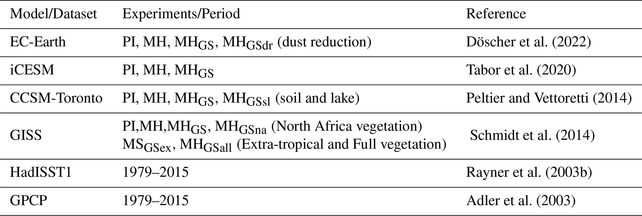

Table 1 Data used in this study.

2.2 Methods

Climate systems are inherently high-dimensional, making their direct analysis challenging. To address this, we apply dimensionality reduction, a standard procedure that projects the system into a lower-dimensional space (a.k.a phase space) while retaining its essential dynamics. In this reduced representation, the climate system evolves along a trajectory. By constructing such trajectories for different climate systems within the same reduced space, we obtain a common framework for comparison. These trajectories encapsulate key aspects of climate variability and dynamical periodicity, which can then be systematically analyzed across systems. In this section, we will present a simplified 2-dimensional solution for the tropical and South Atlantic SST system, enabling us to apply our method more comprehensively.

2.2.1 Dimensionality Reduction – Defining the Phase Space

Principal Component Analysis

Principal Component (PC) analysis (also known as Empirical Orthogonal Functions – EOF) is a technique used to reduce data dimensionality. When studying a high-dimensional dynamical system, such as numerical climate model simulations, finding relevant statistical information that emerges from the system's dynamics can be inefficient and overwhelming (Haykin, 2009). The PC analysis derives a new set of orthogonal coordinates from your data, ordering the EOF patterns that maximize the data's variance in a decreasing fashion, enabling a drastic reduction in dimensionality of your dataset while preserving most of its variation (Jolliffe, 2002). The PC time series is the projection of our data in the corresponding EOF pattern.

In this approach, we extracted two distinct phase spaces (one for SST and another for precipitation) composed of EOFs derived from the combined simulations of all models and scenarios. This process yields a unified phase space with a shared spatial structure for the entire ensemble, providing a consistent framework for analyzing and comparing variability across different simulations (Chandler et al., 2024). This procedure is discussed and applied by Chandler et al. (2024), who construct a merged dataset across models and extract dominant modes of variability using principal component analysis. Their approach implicitly defines a shared low-dimensional representation for inter-model comparison, which is conceptually related to our phase-space construction.

Low frequency filters

To investigate decadal variability in the Atlantic Ocean, decadal filters were applied across all datasets, calculated as simple decadal means from the original monthly time series. These filters serve two primary purposes: first, to examine the decadal coupling between precipitation and SST variables; and second, to extract consistent multi-model patterns that serve as the foundation for a shared phase space. Decadal filtering is applied to the precipitation and SST datasets before pattern extraction to effectively smooth out fine-scale structures and disparities arising from different model architectures. Since we define a single phase space to encompass the merged dataset, this filtering process is essential to ensure that the leading climatic patterns capture substantial variance across the integrated multi-model ensemble.

Atlantic Ocean Modes SST Indices

A more classical approach to reducing the dimensionality of Atlantic Ocean SST and identifying its modes of variability is through the use of SST indices from regional boxes (Deser et al., 2010). Together with pressure gradients and wind anomalies, the ocean modes arising from these SST anomalies induce precipitation in the ocean and adjacent continents (Gorenstein et al., 2023). These indices are constructed from pre-defined spatial boxes and provide a reduced representation of the system by capturing key patterns of tropical and South Atlantic SST decadal variability. In particular, the Atlantic Meridional Mode (AMM: the difference between 15–5° N, 50–20° W and 15–5° S, 20° W–10° E regional boxes), the Atlantic Equatorial Mode (AEM: 3° N–3° S, 20–0° W regional box), and the South Atlantic Subtropical Dipole (SASD: the difference between 30–40° S, 10–30° W and 15–25° S, 0–20° W regional boxes) can be used to define a phase space analogous to that obtained via PC analysis. However, unlike the PC analysis, these indices can be highly correlated, and they have no reciprocal precipitation modes. In our study, this framework is used to compare the system’s decadal SST variability using different techniques to define the phase-space.

2.2.2 The trajectories in phase space

Projecting a simulation series onto the “n” dimensions of our phase space generates a trajectory in that phase space. To elaborate more, we present a simplified 2-dimensional phase space for the SST decadal anomalies of the EC-Earth – PI experiment, using the two leading EOFs from the merged dataset. First, we apply the dimensionality reduction using the PC analysis to find the merged dataset two leading EOFs (Fig. 1a and b). Then, we project the EOFs into the simulation's Atlantic Ocean time series, generating its PCs (Fig. 1c and d). The trajectory of our system in the 2-D continuous phase space is shown in Fig. 1f. Defining negative, neutral, and positive phases for each index, using a threshold linked to Shannon’s Entropy (as described in Sect. 2.3), we coarse-grain this space into n³ states (9 possible states for this 2-D problem). The discrete state evolution of our system (Fig. 1e) is defined by quadrants in the 2-D map (States from Fig. 1f). Finally, the trajectory can also be seen as a discrete system evolving in time, from one possible state to the next, as depicted in Fig. 1g.

Since the continuous trajectory in a high-dimensional phase space can be challenging to plot, the trajectories of a system in a higher-dimensional phase space can be depicted with directed graphs (Figs. 2, 3h and 4h, and 5–8). These graphs can hold different information regarding the system's trajectory in phase space. Each node in these graphs represents a state of the system at a particular time step, with the node's size indicating the number of months the system remained in that state. Nodes that appear darker have a higher degree, meaning they are connected to more transitions to and from other states. This indicates that the system frequently returns to the same state, which results in a darker color for that node. The distance between nodes is irrelevant; it was adjusted for the graph. The information in a directed graph can be overwhelming to analyze for every simulation run; therefore, we utilize its information to calculate a macro-property that reflects its variability in phase space.

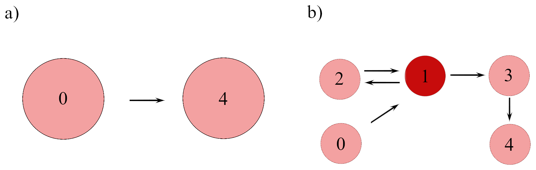
Figure 2 Two abstract directed graphs representing dynamic systems of the same time series length: (a) A system evolves from its initial state (0) to its final state (4) – a low-entropy system. (b) A system evolves from its initial state (0) to state 1, then to state 2, back to state 1, to state 3, and finally to its final state (4) – a high-entropy system.

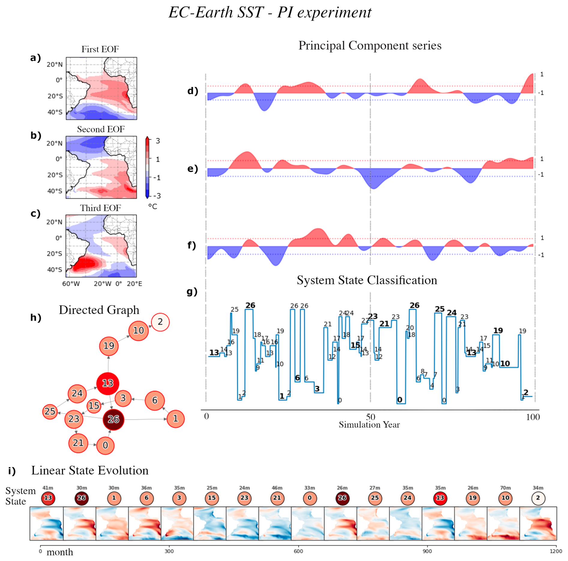
Figure 3 EC-Earth SST state identification and evolution during the PI experiment. Panels (a)–(c) show the merged ensemble’s first three EOF patterns, with (d)–(f) displaying their corresponding PC series (red/blue indicating positive/negative phases; dashed lines showing 1 standard deviation). (g) identifies discrete system states based on these PC indices, bold font used in the most persistent states (lasting more than 24 months); (h) illustrates state evolution of the most persistent states. (i) tracks the state evolution in linear form. Each node displays its cluster number, spatial pattern, and duration in months before transitioning.

2.2.3 Entropy as an analogue for climate variability

Shannon's Entropy (Eq. 1) is used as a measure of variability in unfied the phase space.

$$\begin{array}{}\text{(1)}& H=-\sum _{k=\mathrm{0}}^{N}P\left(x_k\right)\ln \left(P\right(x_k\left)\right)\end{array}$$

The entropy of a dynamic system is a measure of its organization in a coarse-grained space. For example, the systems from Fig. 2a and b have the same initial and final states (0 and 4, respectively); however, system “a” evolves directly from the initial to the final state, while system “b” varies across different states until arriving at the final state. This means that system “a” is less chaotic, its trajectory is more organized, and hence its entropy is smaller.

Looking at Eq. (1), the probability (P(x_k)) of our system x (the simulated Atlantic Ocean SST and precipitation) being found in each possible state (k) can be calculated empirically from the simulation time series. For example, if a specific simulation has been in only one state during its whole time series, that state (x_k) has a probability equal to one to be found in that specific state and zero in the others. Considering that ${\sum }_{k=\mathrm{1}}^{N}P\left(x_k\right)=\mathrm{1}$, the entropy from that time series is the lowest possible, zero. In our study, defining a 3-dimensional phase space and discretizing each dimension in 3 possible phases (positive, negative, or neutral) creates 27 possible states of our system. The entropy from each time series will reflect its variability in that discrete phase space. Since we are using the same space for all the models and scenarios, we can compare their variability.

From a broader perspective, the probability distribution from the Atlantic SST or precipitation patterns (micro-states) in a simulation (trajectory) is used to determine the system's decadal variability (macro-properties) in our unified phase space (the 3 leading EOFs from our merged dataset).

2.3 Phase-Space Discretization Based on Maximum Entropy

The results presented in this study are based on a multi-model analysis using single realizations from each experiment. Because we do not analyze large ensembles of simulations, the conclusions drawn here are strictly conditional on the specific models and experiments considered. Within this context, the uncertainty associated with the entropy estimates arises primarily from the discretization of the principal-component phase space and the representation of its 27 possible states.

The value of Shannon’s entropy depends critically on how the phase space is discretized. Small changes in the thresholds used to define the positive, negative, and neutral phases can substantially alter a simulation’s trajectory through phase space and, consequently, its entropy (see Figs. S2 and S3 in the Supplement). A common approach in the literature is to normalize each principal component by its standard deviation and apply a fixed threshold to define these phases (typically ranging between 0.5 and 1.5). However, climate models differ markedly in their representation of variability due to internal climate fluctuations, differences in numerical formulation and parameterizations, and uncertainties associated with imposed boundary conditions and forcings (Lehner et al., 2020). Applying a single fixed threshold across all models, therefore, risks producing entropy values that reflect differences in simulated amplitudes rather than differences in the temporal organization of variability.

To address this limitation, we adopt an entropy-centered discretization strategy in which the threshold is determined by the requirement of maximizing entropy, rather than prescribing entropy as a consequence of an arbitrary threshold choice. In this formulation, the threshold is allowed to vary between simulations, ensuring that each model’s variability is characterized using the discretization that best represents its exploration of the phase space.

All simulations are projected onto a unified phase space, such that differences in entropy arise solely from how each simulation occupies and transitions between the same set of possible system states. Although we do not explicitly disentangle the relative contributions of internal variability, model structure, and scenario forcing, these effects are implicitly encoded and absorved by this mobile threshold and in the resulting state trajectories. Given the limited number of simulations analyzed, the results should be interpreted as conditional on the specific models and experiments considered, rather than as a comprehensive sampling of model uncertainty.

The maximum entropy of a trajectory is an emergent property of the three-dimensional phase space and corresponds to the threshold that yields the greatest diversity of occupied system states during a simulation. The uncertainty associated with this estimate is quantified using a bootstrap approach.

For each simulation, entropy is evaluated over an interval of candidate thresholds used to define the 27 possible system states associated with the three principal components. The maximum entropy is identified for each time series, and its uncertainty is estimated using a percentile bootstrap method (Hinkley, 1988; Diciccio and Romano, 1988; Gorenstein et al., 2022b). Specifically, 1000 surrogate realizations of each phase space index are generated by resampling from the original dataset of each experiment, and the maximum entropy is recalculated for each realization. The resulting 95 % confidence interval is taken as the uncertainty of the entropy estimate and is used to assess differences in climate variability between simulations.

In climatology, variability encompasses the temporal amplitude fluctuations of a given variable. In contrast, Shannon Entropy, as calculated here, accounts for these variations with an amplitude filter. When we define a phase space using the leading PCs, we select a domain characterized by the patterns representing the system's greatest variance. By normalizing the indices and determining the threshold that maximizes Shannon Entropy, we effectively isolate temporal dynamics from the influence of amplitude variations. Our approach establishes a leveled ground for analyzing the temporal evolution of the system's state across its defining patterns, ensuring that the results remain independent of the specific amplitude differences simulated by various numerical models. In other words, although two models may reproduce the 1st PC with different amplitudes, they are both considered representations of the same climatic pattern. Consequently, Shannon's Entropy evaluates the system's persistence and transitions between states independently of these amplitude variations.

3 Results

We test our methodology in three steps. First, we analyze the outputs of four different numerical climate models in PI and various MH climate scenarios (see Methods). We extract the tropical and South Atlantic SST and precipitation three leading Principal Components (PCs), calculate their trajectory in this 3-dimensional phase space, and compute their respective Shannon Entropy. In the second, we explore the classical Oceanography SST-based indexes to create the Tropical and South Atlantic Ocean's SST phase space (see Methods), calculate its trajectory and Shannon Entropy once again. The third step is a comparison between the calculated entropy values from the model simulations and observational data from satellites using the previously discussed phase spaces.

3.1 The Green-Sahara Simulations in the Principal Component Phase Space

We define the system as the coupled tropical and South Atlantic decadal variability of SST and precipitation. Monthly outputs from 17 simulations across multiple experiments are analyzed, each covering 1200 months on a one-degree resolution grid. To make sure we extract physically meaningful patterns, we create the merged data set's phase-space using the Tropical South Atlantic three leading EOFs (Fig. 3a, b, and c) and project these spatial patterns in each simulations time series, creating their PCs (Fig. 3d, e, and f), we repeat this procedure for precipitation (Fig. 4). For SST, these components explain about 50 % of the total variance across all simulations (21 % from the first PC, 17 % from the second, and 12 % from the third). The three main components share the same spatial pattern as the detrended HadISST1 observation dataset (Rayner et al., 2003b), where they account for 80 % of the total variance from 1979–2015 (42 % from the first, 24 % from the second, and 14 % from the third – Fig. S1).

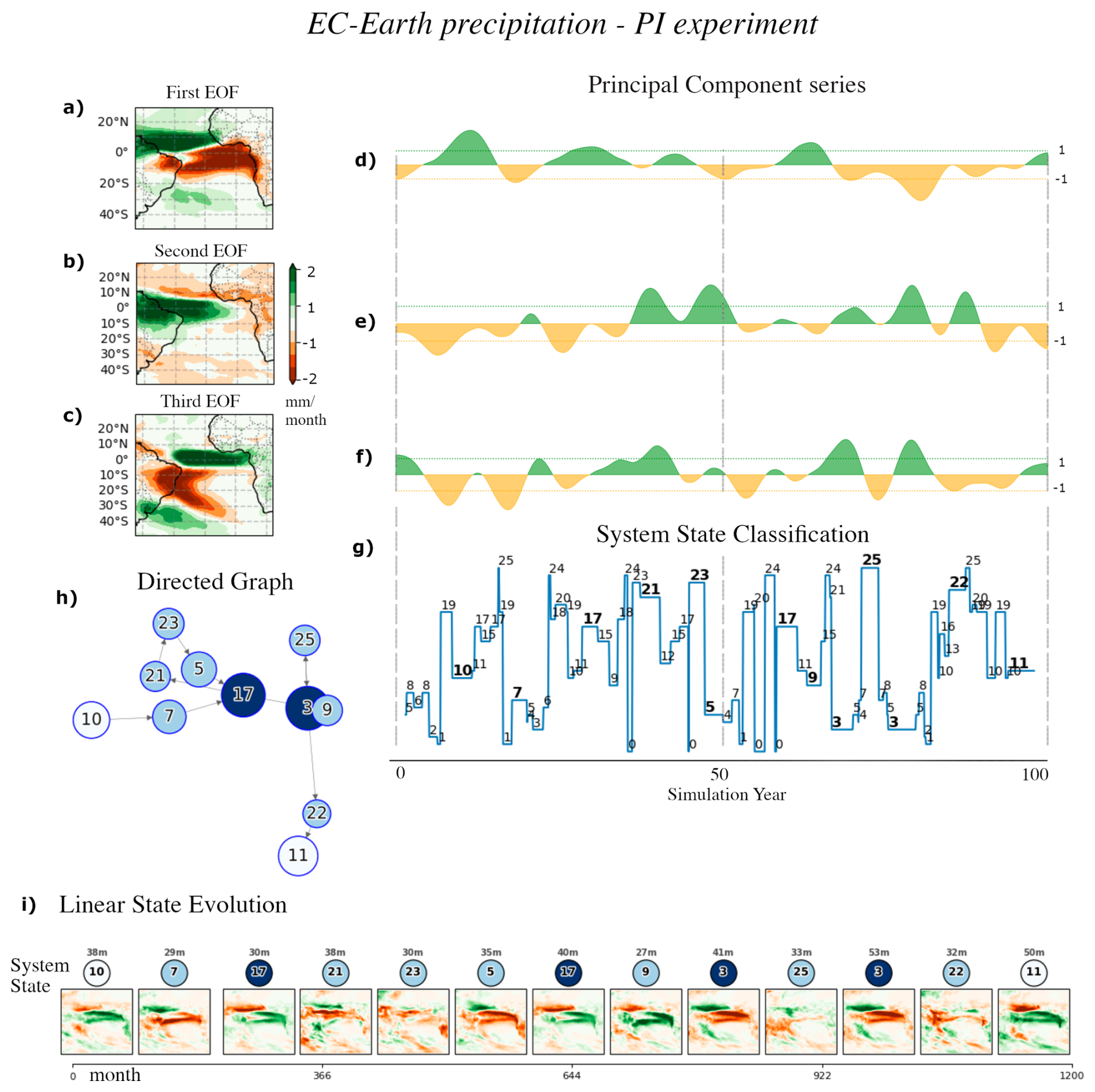
Figure 4 EC-Earth precipitation state identification and evolution during the PI experiment. Panels (a)–(c) show the merged ensemble’s first three EOF patterns, with (d)–(f) displaying their corresponding PC series (green/orange indicating positive/negative phases; dashed lines showing 1 standard deviation). (g) identifies discrete system states based on these PC indices, bold font used in the most persistent states (lasting more than 24 months); (h) illustrates state evolution of the most persistent states. (i) tracks the state evolution in linear form. Each node displays its cluster number, spatial pattern, and duration in months before transitioning.

To transform this continuous space into a discrete space, we divide each PC index into three phases (positive, negative, and neutral), defining the 27 possible states in which our system's SST can be found (Fig. S2), and constructing a discrete trajectory in phase space (Figs. 3g, h, and i and 4g, h, and i).

In Figs. 3 and 4, the EC-Earth PI experiment is used to illustrate how the PC indices correlate with its trajectory. However, this choice is not particularly significant. All other graphs (Figs. 5, 6, 7, and 8) follow a similar construction and yield comparable results.

3.1.1 Directed Graphs

Each simulation run can be represented as two trajectories in the PC phase spaces, one for the SST and one for precipitation. These trajectories of the Tropical and South Atlantic system (fully depicted for EC-Earth in the System State Classification “g” from Figs. 3 and 4) are formed by all the states a system occupies during its time series. However, it can be challenging to present this information due to the high number of states and transistions. Even in a low 3-dimension phase space, it can be overwhelming to represent the full trajectory in a plain figure. Therefore, we chose to represent the most persistent states a system occupies (depicted in bold numbers in “g” from Figs. 3 and 4) in the directed graph form for each simulation experiment (Figs. 5–8). In Figs. 3 and 4, the direct graph can be seen in its ciclycal and linear forms (“h” and “i”, respectively). These graphs qualitative ilustrate the ciclicity and organization of a simulation, furthermore, their construction uses quantitative measures of the system in the phase-space. Each node in these graphs represents a system state at a given time step, with its size indicating the duration spent in that state, and its color intensity reflecting the frequency of transitions to and from other states (higher degree). Darker nodes indicate states the system revisits more often. The same properties used to design each graph were employed to calculate macroproperties such as the entropy of the time series.

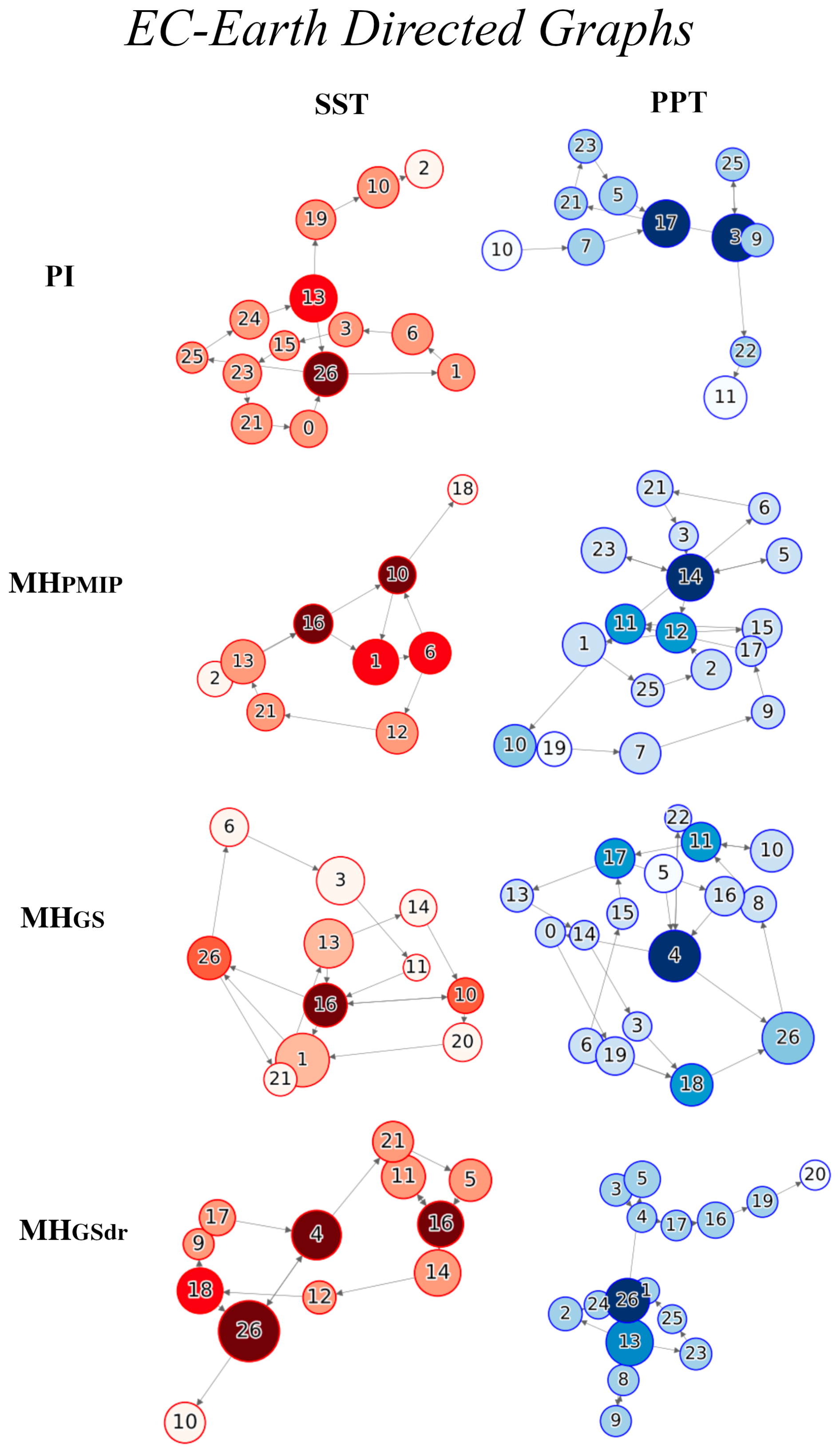
Figure 5 Directed graphs from EC-Earth – PI, MH_PMIP, MH_GS, and GS with dust reduction (MH_GSdr) simulations. The red graphs represent the SST system evolution, and the blue graphs represent the precipitation evolution. Each node signifies a specific state, as depicted in Fig. S2.

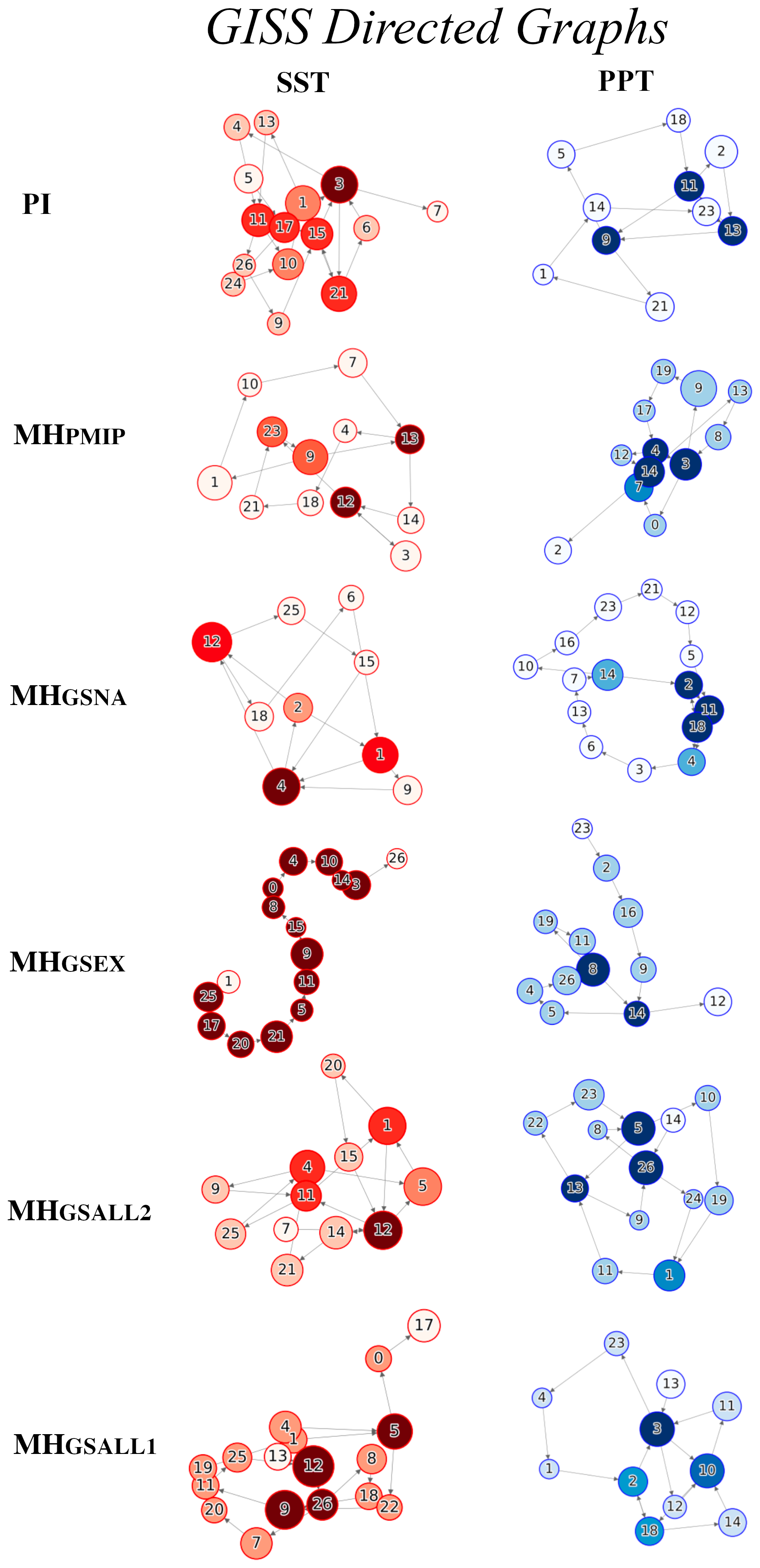
Figure 6 Directed graphs from GISS - PI, MH_PMIP, MH_GS with North Africa (MH_GSNA), Extra-Tropical (MH_GSEX), and full vegetation (MH_GSALL1 and MH_GSALL2) runs. The red graphs represent the evolution of the SST system, while the blue graphs represent the evolution of precipitation. Each node signifies a specific state, as depicted in Fig. S2.

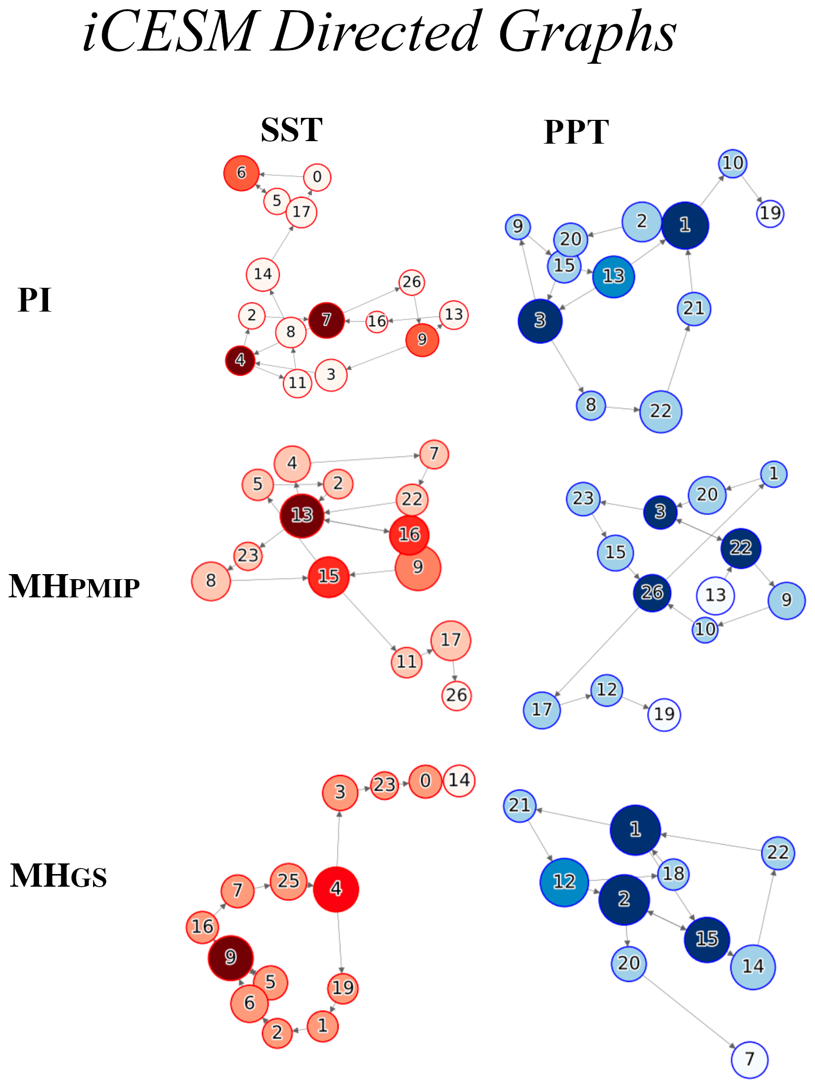
Figure 7 Directed graphs from iCESM – PI, MH_PMIP, and MH_GS runs. The red graphs represent the SST system evolution, and the blue graphs represent the precipitation evolution. Each node signifies a specific state, as depicted in Fig. S2.

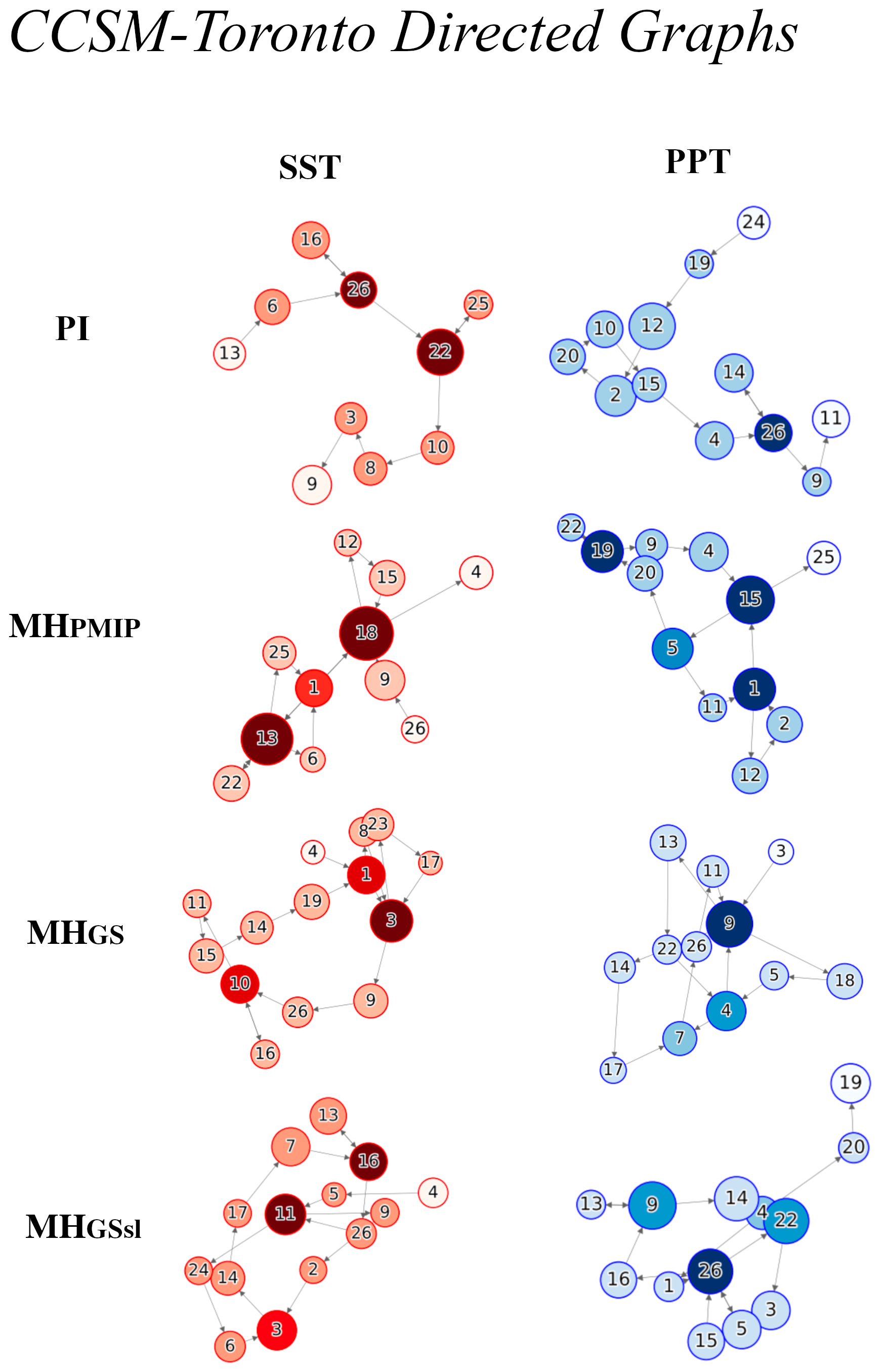
Figure 8 Directed graphs from CCSM-T – PI, MH_PMIP, MH_GS, and MH_GSsl with soil and lake input runs. The red graphs represent the evolution of the SST system, while the blue graphs represent the evolution of precipitation. Each node signifies a specific state, as depicted in Fig. S2.

Shannon's Entropy and Model Variability Analysis

In this study, Shannon's Entropy (H_sst and H_ppt) is used to assess the level of organization of the tropical and South Atlantic given its possible states (as described in Eq. 1).

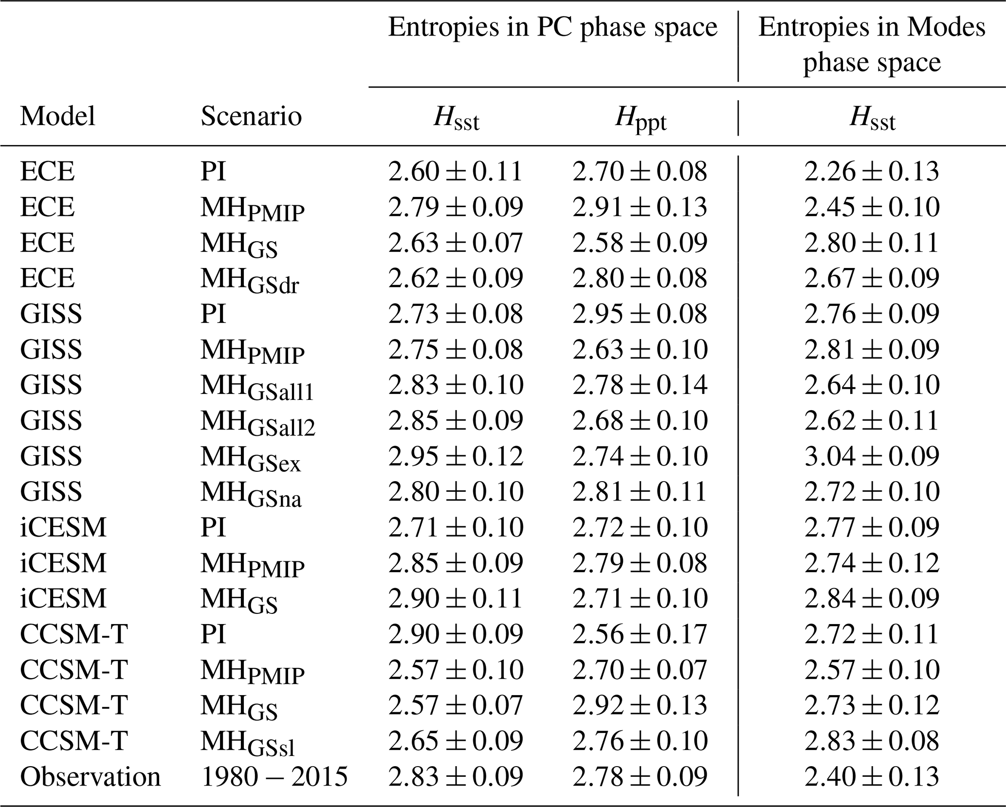
Our choice to study decadal variability stems from the coupling between SST and precipitation at this time scale (Gorenstein et al., 2023). Since these two variables are correlated and exhibit a strong feedback interaction controlling the energy balance along the Equator (Schneider et al., 2014), we expect them to vary together, creating a distinguishable climate variability response to external forces. The first two columns of Table 2 show the entropy calculated in the PC phase space and its 95 % confidence interval for each model experiment. Despite differences in parameterizations and physics among models, each entropy was computed in a unified space (the states of every simulation were calculated using the EOFs extracted from the merged dataset). All model experiments were simulated over the same duration (100 years), enabling comparisons across the different models.

Table 2 Entropy mean and Standard Deviation using 1200 months long series from the model runs – calculated in the PC and Atlantic Ocean Modes phase spaces.

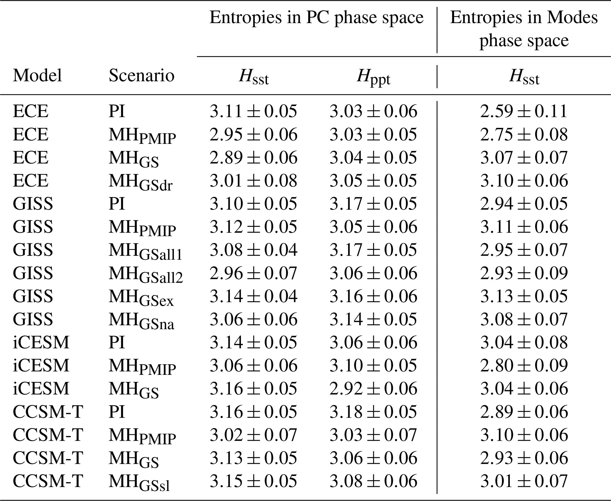
As seen in Fig. 9 and Table 2, the entropy values are approximately 3. This is due to the structure of our phase space: with three defined phases (positive, neutral, and negative) for each of the three principal components, the system has 3³ = 27 possible states. The maximum entropy (Eq. 1) of a discrete space such as this would result in ln(27) ≈ 3.296. Since the simulation’s thresholds in phase space are individually tuned to yield its maximum possible entropy (see Methods), it naturally approaches ln(27).

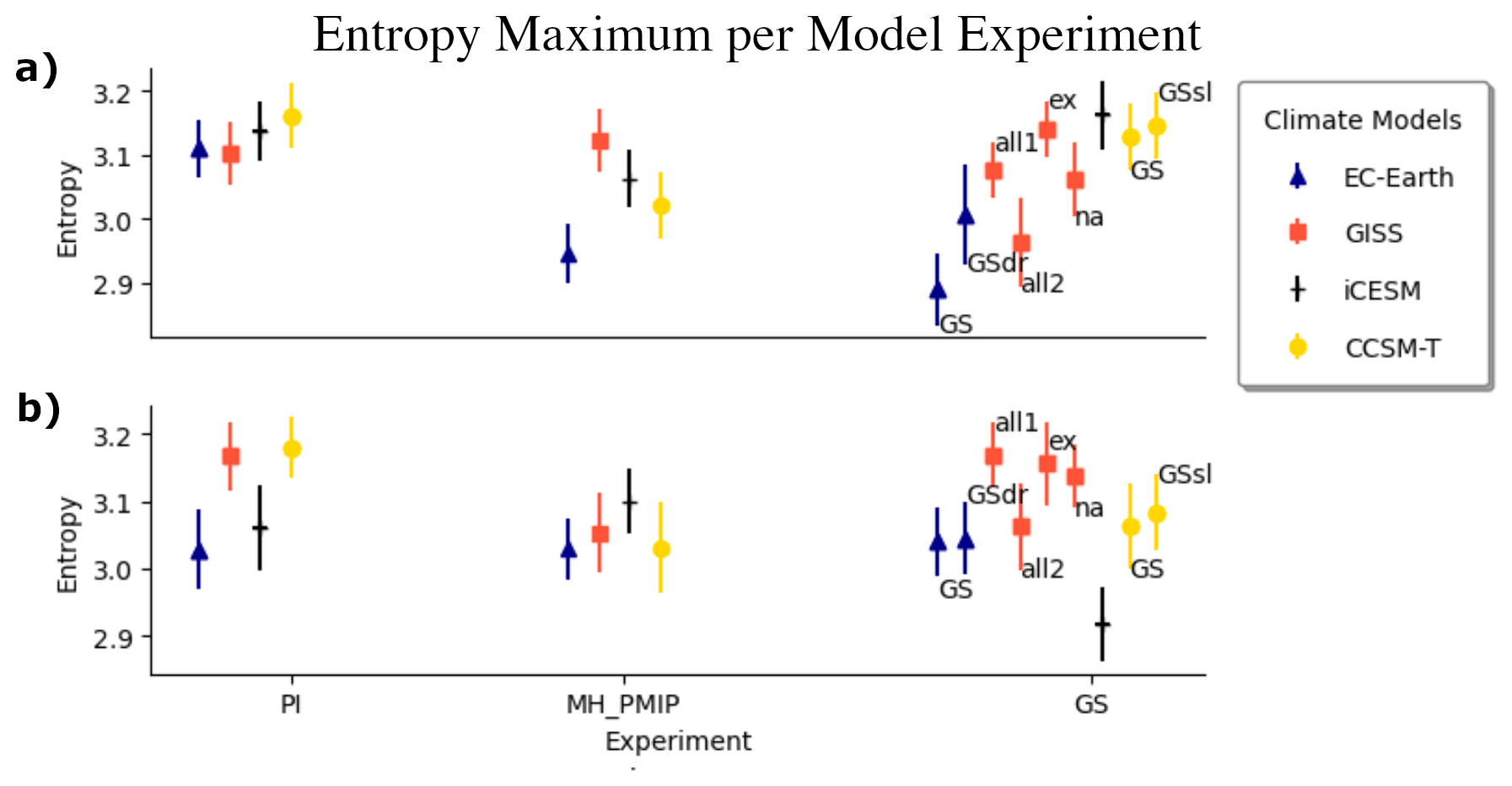
Figure 9 Plot representation of values depicted in Table 2. Maximum Entropy values and uncertainty for each model experiment using the Atlantic Ocean PCs phase space, (a): for SST; (b) for precipitation. From left to right: Pre-Industrial (PI); mid-Holocene only orbital forcing (MH_PMIP); and mid-Holocene with Green Sahara boundary conditions (MH_GS) experiments. All models include PI, MH_PMIP, and MH_GS runs. Under Green Sahara conditions, additional experiments include: EC-Earth (ECE) with northern African vegetation and dust reduction (dr); GISS with both extratropical and northern African vegetation (GISSall1 and GISSall2), with only extratropical vegetation (GISSex), and with only north African vegetation (GISSna); CCSM-T with soil and lakes (sl).

EC-Earth

EC-Earth's SST variability significantly drops from PI to the different MH scenarios (it reduces 5 % in MH_PMIP and 7 % in MH_GS in comparison to the PI), when dust reduction is applied its entropy recovers back to PI levels. The lowest SST entropy of all models and scenarios is measured during EC-Earth's MH_GS (blue triangles in Fig. 9a), indicating that in this scenario the EC-Earth model simulates a more organized Atlantic SST system. The precipitation variability shows no significant changes through all the different scenarios (blue triangles in Fig. 9b).

GISS

Compared to the PI experiment, GISS exhibits significant changes in both SST and precipitation variability in the MH_GSall2 experiment (5 % in comparison to the PI). Besides this simulation, only MH_PMIP shown significant precipitation variability decrease when compared to PI. In this model, the largest entropy difference comes from SST in MH_GSall2 and MH_GSex (2.96 and 3.14, respectively – Table 2).

iCESM

For this model, the lowest decadal SST variability happens in the MH_PMIP experiment (black hyfen in Fig. 9), although without significant difference between the scenarios. The precipitation entropy shows significant decrese when vegetation is considered in the Sahara, MH_GS is the lowest of all simulations and scenarios (4 % lower than the PI experiment and 6 % lower than the MH_PMIP).

CCSM-Toronto

The decadal SST variability is higher in the PI experiment, but only significantly different from the MH_PMIP experiment (4 % lower than the PI). Conversely, the MH_PMIP, MH_GS and MH_GSsl present 5 % lower than PI precipitation variability.

3.2 The Green-Sahara Simulations in the Atlantic Ocean Modes' Phase Space

PC-based modes can sometimes blend physical processes or show sensitivity to the chosen spatial and temporal domains, requiring careful interpretation (Preisendorfer and Mobley, 1988). An alternative approach to reducing Atlantic SST dimensions into a 3D phase space uses regional SST indices. These averages provide simple, physically interpretable metrics of climate mode strength. To test how phase space definitions affect Shannon's Entropy, we repeat our calculations using indices for the Atlantic Meridional Mode, the Atlantic Equatorial Mode, and the South Atlantic Subtropical Dipole (AMM,AEM and SASD, see Methods); representing Atlantic decadal variability through a traditional oceanographic lens (Deser et al., 2010).

In the merged dataset, the first PC correlates strongly with the AEM (70 %) and SASD (64 %), while the second PC correlates with the AMM (71 %). However, while the SST indices are significantly intercorrelated (39 %–43 % in the merged dataset), the PCs maintain negligible correlation (below 3 %). As an orthonormal basis, PCs inherently ensure minimal correlation between dimensions, unlike regional indices. This index-based phase space yields generally lower entropy values than the PC-based space. While Shannon Entropy does not directly measure correlation, if two PCs are correlated, their positive, neutral and negative phases vary togheter and the system ocuppies less states, resulting in lower entropy values.

3.2.1 EC-Earth

The EC-Earth PI experiment (Fig. 10) best illustrates how high correlation results in low entropy, showing the lowest entropy of all simulations within the Atlantic Ocean Modes phase space. In this specific setup, the AEM and AMM are correlated at 88 %, while the AMM and SASD show a 76 % correlation. Conversely, all MH scenarios exhibit higher entropy than the PI (6 % for MH_PMIP and 19 % for GS with/without dust) as these Atlantic modes decouple.

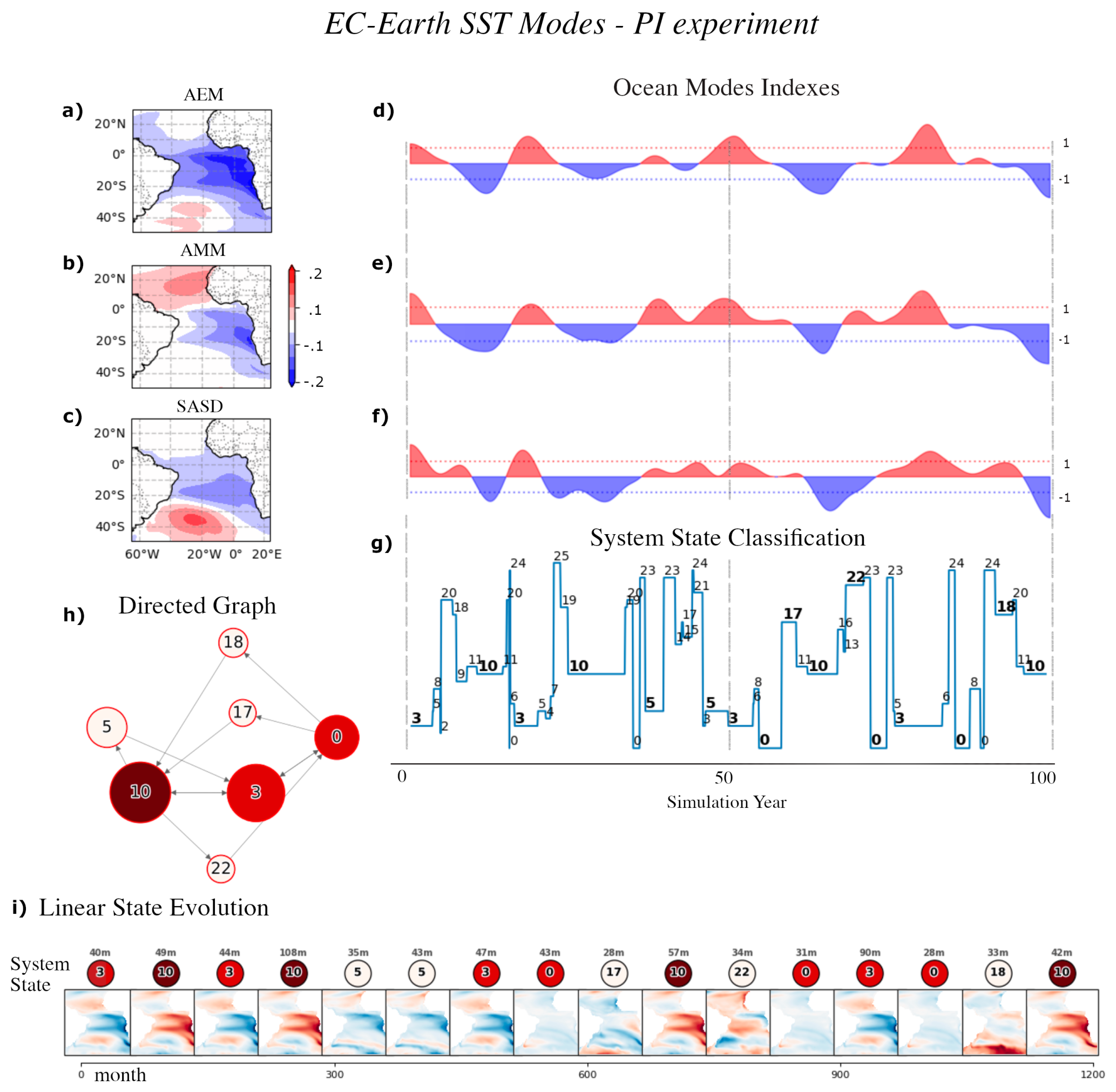
Figure 10 EC-Earth SST system state identification and evolution during the PI experiment. (a), (b), and (c) The merged ensemble AMM, AEM, and SASD, respectively; (d), (e), and (f): their respective index series, blue for negative and red for positive, dashed lines indicating the 1 standard deviation value. (g) The cluster identification of the discrete system state given the three above Ocean Mode indices, bold font used in the most persistent states (lasting more than 24 months); (h) illustrates state evolution of the most persistent states. (i) tracks the state evolution in linear form. Each node displays its cluster number, spatial pattern, and duration in months before transitioning.

3.2.2 GISS

Compared with the PC phase space, GISS PI entropy reduces using the Atlantic ocean modes indices (Table 11). The entropy from the remaining MH scenarios mostly decreases; however, they show no significant changes to the entropies calculated in the PCs phase space.

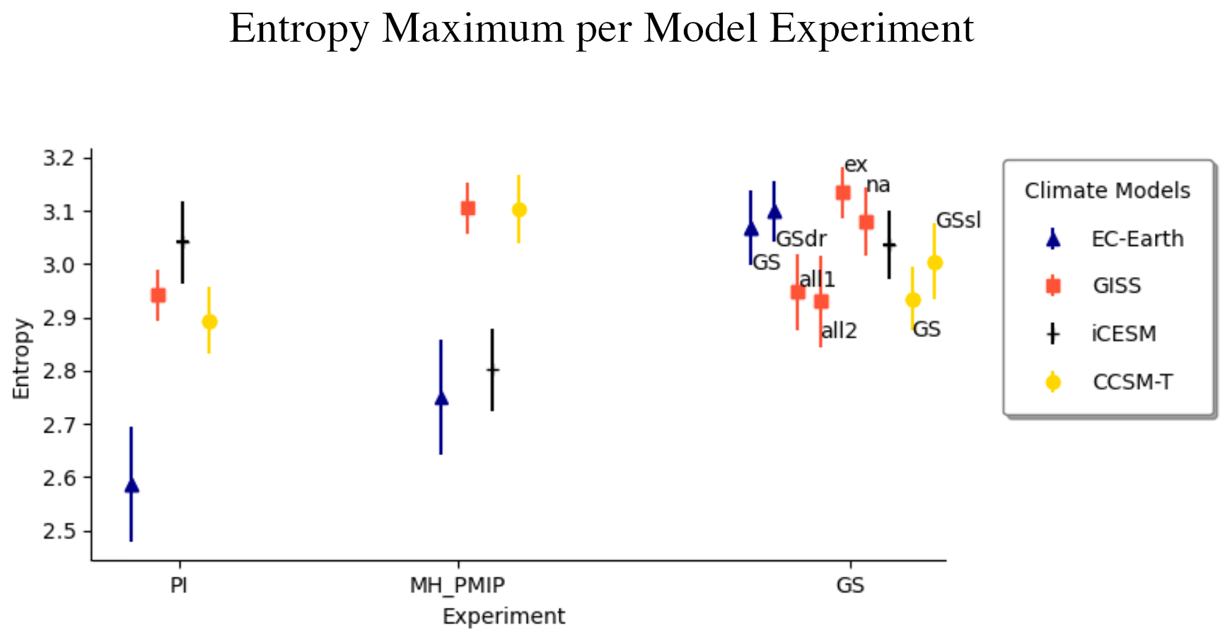
Figure 11 Maximum Entropy values and uncertainty for each model experiment for SST using the Atlantic Ocean modes phase space. From left to right: Pre-Industrial (PI); mid-Holocene only orbital forcing (MH_PMIP); and mid-Holocene with Green Sahara boundary conditions (MH_GS) experiments. All models include PI, MH_PMIP, and MH_GS runs. Under Green Sahara conditions, additional experiments include: EC-Earth (ECE) with northern African vegetation and dust reduction (dr); GISS with both extratropical and northern African vegetation (GISSall1 and GISSall2), with only extratropical vegetation (GISSex), and with only north African vegetation (GISSna); CCSM-T with soil and lakes (sl).

3.2.3 iCESM

For this model, the SST entropies show a general decrease, while holding the same internal biases seen in the PC phase space entropies (Table 11).

3.2.4 CCSM-Toronto

The only significant difference is still between PI and MH_PMIP; however, in this phase space, MH_PMIP holds the largest entropy amongst this model's different experiments (7 % higher than PI).

3.3 The Observational data Entropy

A primary goal of numerical climate models is the faithful reproduction of low-frequency decadal variability. Notable differences exist between the PCs extracted from observational data and model data, nor do they represent the same variance as the principal components from the leading components seen in the observational satellite era (Fig. S1). However, the EOFs extracted from the merged simulations dataset can be projected onto the observational data time series. As long as they have the same length, the use of maximum Entropy enables a comparison between the observational data and the simulations' trajectories in a common phase space. Since the observational datasets range from 1980 to 2015, the results shown in the Table ahead are the Entropy values of the first 420 months (35 years) of each simulation. Within these time windows, the resulting entropy values are lower, indicating that shorter intervals do not fully capture the decadal variability envelope of the tropical and South Atlantic system.

Typically, satellite-era observations are compared against historical model runs. Previous research categorized the tropical and South Atlantic systems into a discrete evolution of patterns, tracking the SST and precipitation cycles using reanalysis data from 1890–2015 with a directed graph format (Gorenstein et al., 2023). However, as an attempt to quantitatively compare the values emerging from the numerical climate models' entropy in these MH experiments, we calculate the entropy from two observational datasets (the HadISST and the GPCP datasets - see Methods). These values are presented in Table 3.

Table 3 Entropy mean and Standard Deviation from the 420-months-long series model runs and the observation data set.

In the PC phase space, the ensemble model mean (2.76 for SST and 2.75 for precipitation) falls within the observational entropy uncertainty interval. However, in the Atlantic Ocean Modes phase space, the ensemble model mean (2.70) is significantly higher than the observational entropy value (2.40±0.13). While this could suggest that historical variability is lower than most of the PI and MH experiments presented, such a direct comparison assumes the models represent these modes accurately. Instead, this discrepancy may indicate that, for this methodology, studying Atlantic decadal variability in simulations is more reliable when using principal components rather than traditional SST indices.

4 Discussion

The core purpose of the developed methodology is to evaluate and compare the temporal variability of a physical system across different scenarios. For the tropical and South Atlantic specifically, pre-Industrial and mid-Holocene runs were chosen because they provide a period where multiple known forcings (such as insolation and vegetation) can be used to study the coupling and decadal dependencies between SST and precipitation.

The standard approach to analyzing these climate variables variability in climate reconstructions using numerical model simulations is to compute the two-dimensional mean and standard deviation fields, and frequency spectra (Flato et al., 2014; Olonscheck and Notz, 2017; Pendergrass et al., 2017; Bianchini et al., 2025). This approach accounts for the local dependencies of climate variables, where the standard deviation fields indicate the amplitude of regional variability, and the frequency spectra reveal periodicity.

There is no trivial path to compare our results with the standard methodology, as the underlying concepts used to define climate variability differ, and although its not the main purpouse of our methodology, we can use it to validate the model climate simulations with proxy information. Previous studies have used biochemical proxy data from sediment and ice cores to examine mid-Holocene climate variability in the Tropical and South Atlantic (Debret et al., 2009; Wirtz et al., 2010). Wirtz et al. (2010) found generally lower precipitation variability than at present, except for the Northeast Brazil coast, where variability increased. Numerical models have also simulated ocean mode indices and monsoon changes in Africa and the Americas using mid-Holocene forcings (Harrison et al., 2003; Zhao et al., 2007). Specifically, Zhao et al. (2007) analyzed nine PMIP2 models, finding reduced Sahel precipitation variability and weakened teleconnections between Pacific/Atlantic SSTs and Tropical Atlantic precipitation, suggesting a decoupling of these variables.

In our study, most model responses show lower tropical and South Atlantic SST variability during the mid-Holocene when using only insolation parameters; specifically, all MH_PMIP models exhibit lower Entropy than MH_PI, except for GISS, which shows equivalent values (Fig. 9). However, only GISS and CCSM-T show lower precipitation variability in MH_PMIP compared to MH_PI. When Green Sahara vegetation is factored in, a decoupling between SST and precipitation variability becomes clearer in three of the four models: EC-Earth, iCESM, and CCSM-T show significantly larger entropy differences between the variables, though EC-Earth displays low SST entropy with high precipitation, while CCSM-T and iCESM show the reverse. In contrast, the GISS model keeps the variables more closely coupled, with no significant entropy differences across scenarios.

Measuring decadal variability in climate models typically relies on statistical methods common in data science to pinpoint regions highly susceptible to change, thereby aiding in the regional validation of models against observational data. However, recent research utilizing information theory suggests that traditional variance-based estimates can be unreliable when accounting for non-Gaussian higher statistical moments. Consequently, there is a growing need for variability metrics that remain robust regardless of a variable's amplitude or units of measurement (Sane et al., 2024). Our methodology measures a region's decadal climate variability concerning the chosen phase space (ocean modes of variability and their precipitation counterparts). Although we have shown that it is more straight forward to use the leading PCs of SST in the tropical Atlantic Ocean for the absense of correlation between its orthonormal components, they still alow us to study the Atlantic Ocean Modes as conceptualized in the classical oceanography, climatology, and dynamic systems theory (Deser et al., 2010; Ghil and Lucarini, 2020; Cheung et al., 2026).

Modes such as El Niño, the AMM, and the AEM influence climate across the globe; they are known to impact society (McGowan et al., 2012; Lam et al., 2019), agriculture (Anderson et al., 2018), the atmosphere (Xie and Carton, 2004; Gorenstein et al., 2023), and climate equilibrium (Pillai et al., 2022; Cai et al., 2021). The temporal evolution of these modes provides a conceptual framework for measuring decadal climate variability in numerical models using the same metrics applied to observational datasets. Accordingly, the phase space used to compute Shannon entropy is constructed to explicitly reflect the variability associated with these climate modes. Although we employed standard deviation to define the positive, neutral, and negative phases of the Atlantic modes, it is not necessarily the case that a simulation with high regional standard deviation (the traditional measure of climate variability) will correspond to a high entropy measurement.

5 Conclusions

We introduce a information-theoretic framework to characterize the organization and variability of climate systems. We demonstrate our methodology by analyzing the tropical and South Atlantic SST and precipitation decadal variability across four climate models (EC-Earth, GISS, iCESM, and CESM-Toronto) simulating the PI, mid-Holocene experiments and observational data from the satellite era (HadISST and GPCP). Representing SST and precipitation as trajectories in a unified physically motivated low-dimensional phase space, we describe the tropical and South Atlantic climate system in a course-grained space of 27 possible states. In this discrete space, we compute Shannon’s entropy, accesing how organized the coupled ocean–atmosphere system is under PI and different MH boundary conditions.

Across four models, the results show that mid-Holocene forcings can significantly alter the degree of organization of Atlantic decadal variability, with model-dependent entropy changes, and different SST and precipitation responses. Comparisons with observational datasets indicate that PC-based phase spaces provide a more consistent and robust basis for evaluating low-frequency Atlantic variability than traditional SST indices, highlighting entropy as a powerful metric to diagnose how external forcings reshape the structure, persistence, and transitions of dominant climate modes.

EC-Earth shows the strongest reduction in SST entropy under Green Sahara conditions, indicating a more organized and persistent Atlantic Ocean system that is partially reversed when dust reduction is included, while its precipitation variability remains largely unchanged. GISS displays a spread in entropy responses, with the MH_GSall2 simulation exhibiting significant reductions in both SST and precipitation entropy, highlighting the sensitivity of Atlantic variability to ocean–atmosphere coupling in this simulation. In contrast, iCESM exhibits comparatively muted SST entropy changes across scenarios but a clearer precipitation response under Green Sahara forcing, whereas CCSM-Toronto shows a tendency toward reduced precipitation variability across all mid-Holocene experiments, with weaker and more selective SST changes. Taken together, these results indicate that while the direction and magnitude of entropy changes depend on model physics and boundary-condition implementation, all models encode distinct and interpretable reorganizations of Atlantic decadal variability under altered Holocene climates.

Because this study is based on single realizations, differences in entropy between experiments may reflect a combination of sensitivity to initial conditions and differences in boundary conditions or parameterized processes. Applying this methodology to ensemble simulations or emulators that systematically perturb initial conditions and external forcings (e.g., dust or vegetation) represents a natural extension of this work and would enable a more rigorous assessment of how Shannon entropy responds to different climate variables and scenarios.

This methodology characterizes system dynamics and variability in terms of state occupancy and transitions rather than absolute anomaly magnitudes. By discretizing the climate system in a unified low-dimensional phase space and computing Shannon’s Entropy, the underlying climate variability can be directly compared between different models, experiments, and observations. The approach captures how frequently the system revisits certain states, how persistent those states are, and how rich the transition structure is, all of which are fundamental aspects of variability that are not accessible through variance-based metrics alone. Moreover, because entropy is computed in a common phase space using the maximum entropy threshold, it provides a unified and scale-independent measure of organization that remains robust even when models differ in mean state, variance, or bias, thereby complementing traditional and well-established statistical diagnostics. This makes the framework especially powerful for inter-model comparisons and for evaluating low-frequency climate variability across non-homogeneous datasets.