G6-1.5K-MCB: Marine Cloud Brightening scenario design for the Geoengineering Model Intercomparison Project (GeoMIP) in CESM2.1, E3SMv2.0, and UKESM1.1

We present a protocol for scenario simulations of marine cloud brightening (MCB) solar radiation modification (SRM), which we design for inclusion as a bridge simulation in the Geoengineering Model Intercomparison Project (GeoMIP). This protocol, named G6-1.5K-MCB, parallels the existing G6-1.5K-SAI, but it simulates injecting sea salt aerosol (iSSA) into the lower marine boundary layer to create a MCB scenario. Using information taken from recent modeling studies, we propose to apply MCB iSSA emissions in the midlatitudes, which can produce a surface temperature response that more closely resembles the opposite of the greenhouse gas (GHG) warming pattern without invoking the La Niña response that has been predicted in previous studies. In many ways, this approach is analogous to the choice of emissions at 30° N and 30° S for stratospheric aerosol injection (SAI) in G6-1.5K-SAI. Owing to substantial uncertainty in the aerosol-cloud forcing from MCB, we outline recommended benchmark simulations to facilitate similar simulations of cloud brightening across different models. We present simulations of the G6-1.5K-MCB protocol using three Earth System Models (ESMs). All three ESMs show that for an intermediate baseline GHG emission trajectory, midlatitude MCB can maintain 21st century global mean surface temperature (GMST) at 2020–2039 temperatures. The iSSA emission rates required to maintain this target vary by a factor of 20 across the ESMs due to differences in the size distribution of the emitted iSSA and in the representations of aerosol-cloud interactions, demonstrating the importance of benchmark simulations for both understanding uncertainties and setting up the scenario simulations. Temperature and precipitation anomalies are greatly reduced relative to the GHG warming background, with most regions experiencing no statistically significant changes relative to the reference period. In some regions, there is a notable seasonal cycle in the residual climate change, though the anomalies are still much smaller than the GHG warming impact. On the basis of the promising results from this three-model testbed, we propose that the G6-1.5K-MCB serve as a basis for future model intercomparison protocols. This will enable further estimation of the structural uncertainties of ESMs in the climate response to MCB and provide a valuable dataset for more detailed analysis of the potential impacts of MCB.

1 Introduction

Solar radiation modification (SRM) climate interventions have been subject to increasing scientific interest in recent years owing to their potential to offset the impacts of greenhouse gas warming by reflecting a portion of incoming solar radiation. National and international assessments have made clear there is a need to better understand the feasibility, risks, benefits, and policy implications of SRM technologies (National Academies of Sciences, Engineering, and Medicine, 2021; Feingold et al., 2022; United Nations Environment Programme, 2023). Marine cloud brightening (MCB) is an approach to increase sunlight reflection and cool climate by injecting sea salt aerosols (iSSA) into the lower marine atmosphere (Latham et al., 2008; Feingold et al., 2024) with the goal of making clouds more reflective. The idea is that the iSSA serve as cloud condensation nuclei (CCN), leading to clouds with smaller and more numerous cloud droplets. This change can increase the albedo of the clouds and reduce the amount of sunlight reaching Earth's surface, which we refer to as the cloud albedo effect and is also known as the Twomey effect (Twomey, 1977). Increased cloud droplet number concentration (CDNC) further affects clouds by reducing the rate of precipitation formation, which leads to cloud adjustments via longer cloud lifetime (the cloud lifetime effect – Albrecht, 1989) and by changing cloud and droplet dynamics, leading to cloud thickening or thinning, depending on cloud conditions (e.g., Wood, 2007; Mülmenstädt et al., 2024). Together these processes are referred to as aerosol-cloud interactions or indirect aerosol effects (F_aci). Modeling and observational evidence from analogues of MCB, such as particle emissions from shipping and volcanic eruptions, suggest that MCB could produce substantial climate cooling (Malavelle et al., 2017; Toll et al., 2019; Christensen et al., 2022; Chen et al., 2022; Yuan et al., 2022; Diamond, 2023), but the extent of the potential cooling and the impacts of increasing cloud reflectivity in different ocean regions are still uncertain.

Studies with Earth system models (ESMs) suggest that iSSA can achieve substantial cooling through its impact on clouds and, in some models, marine sky brightening (MSB) driven by the scattering of sunlight by the iSSA itself i.e., through aerosol–radiation interactions or direct aerosol forcing, F_ari (Ahlm et al., 2017; Haywood et al., 2023; Rasch et al., 2024). Thus, iSSA injection could be a complement to emissions reductions that would offset some impacts of global climate change. ESMs suggest that the climate response to MCB depends strongly on the location(s) where MCB is applied (Jones et al., 2009; Hill and Ming, 2012; Rasch et al., 2024; Hirasawa et al., 2026, hereafter H2026). Past modeling has largely focused on MCB implementation in the subtropical east Pacific and Atlantic oceans, due to the extensive coverage of marine stratocumulus clouds in these regions and the high susceptibility of those stratocumulus clouds to brightening by aerosol increases. However, ESMs consistently show strong La Niña-like climate responses to MCB interventions in these regions, and this response can result in highly inhomogeneous regional temperature responses and shifting precipitation patterns (Jones et al., 2009; Rasch et al., 2009; Hill and Ming, 2012; Hirasawa et al., 2023; Rasch et al., 2024; Chen et al., 2024b; Odoulami et al., 2024). Thus, while subtropical stratocumulus MCB may be suitable in terms of achieving efficient brightening and global-scale cooling, ESMs suggest it could also produce undesirable climate responses.

Other ESM studies indicate that shifting the implementation of MCB to the midlatitudes tends to produce more spatially uniform cooling patterns (Baughman et al., 2012; Chen et al., 2024a, H2026), with few regional temperature anomalies and less dramatic precipitation shifts compared to subtropical MCB simulations. Furthermore, the ESM simulations presented in H2026 indicate that midlatitude MCB – in five midlatitude regions: North Pacific – NP [30N to 50° N; 170° E to 120° W], North Atlantic – NA [30 to 50° N; 70 to 0° W], South Pacific – SP [50 to 30° S; 170 to 90° W], South Atlantic – SA [50 to 30° S; 55° W to 15° E], and South Indian Ocean – SI [50 to 30° S; 30 to 100° E] – could produce both efficient cloud brightening and a stronger cooling response for a given amount of brightening than would MCB intervention in the subtropics, due to stronger positive cloud and albedo radiative feedbacks in these regions (Liu et al., 2018a, H2026). By combining iSSA emissions across Northern and Southern Hemisphere midlatitude ocean regions, we found that midlatitude MCB produces a cooling pattern that is anti-correlated with the greenhouse gas (GHG) warming pattern across three models (H2026). This suggests that midlatitude MCB could offset the GHG warming effectively without inducing undesirable regional climate impacts, in contrast to subtropical MCB (Rasch et al., 2024; Chen et al., 2024b).

In this study, we use the midlatitude MCB strategy identified in H2026 to design MCB intervention scenarios in which global mean surface temperature increases are held to approximately 1.5C of warming above preindustrial, defined as the 2020–2039 mean temperature following G6-1.5K-SAI protocol (Visioni et al., 2024). These types of scenario simulations are vital for supporting policy-relevant climate impacts analyses of SRM (MacMartin et al., 2022). There has been extensive development and study of this type of scenario simulations for SAI, such as those developed for the Geoengineering Model Intercomparison Project (GeoMIP – Visioni et al., 2024), the Geoengineering Large Ensemble (GLENS – Tilmes et al., 2018), and the ARISE-SAI protocol (Assessing Responses and Impacts of Solar intervention on the Earth system with Stratospheric Aerosol Injection – Richter et al., 2022). These efforts have provided vital information about the sensitivity of the climate response to the details of SAI deployment, such as the injection locations, target temperature, and start date of the intervention. Furthermore, they have enabled a rich literature on potential impacts of SAI across regions and climate system components.

In contrast, there have been relatively few studies that have simulated hypothetical future scenarios in which MCB interventions are applied. Many MCB studies have used large step-change perturbations aimed at increasing the signal strength to understand the processes and dynamics underlying the response to MCB (Jones et al., 2009; Hill and Ming, 2012; Kravitz et al., 2013; Rasch et al., 2024; Chen et al., 2024a, H2026). Fewer MCB studies have used simulation designs that are more suitable for impacts analysis in which MCB forcing is increased gradually to represent a hypothetical future deployment trajectory, which we refer to as ”scenario” simulations. Alterskjær et al. (2013), for example, evaluated a GeoMIP scenario (G3-SSCE) in 3 coupled climate models in which iSSA was emitted into the tropics between 30° S and 30° N and the emissions were scaled to maintain the top of atmosphere radiative forcing to RCP4.5 2020 levels. Two of the three ESMs in that study did not include important treatments of some aerosol-cloud interactions for the accumulation mode iSSA particles used for MCB, so it was necessary to use iSSA and CDNC fields from one model, NorESM, in the other two models resulting in some inconsistencies between the meteorology and iSSA/CDNC fields in those models. Furthermore, the tropical MCB strategy used in the study tended to under-cool higher latitude regions and over-cool the tropics (Aswathy et al., 2015). More recently, Haywood et al. (2023) and Lee et al. (2025) simulated scenarios using variations of subtropical MCB intervention strategies. In Haywood et al. (2023), iSSA were added into four regions in the Eastern Pacific and increased over time to take the global mean temperature trajectory from SSP5-8.5 to SSP2-4.5. This resulted in a strong La Niña-like cooling in the Pacific which shifted circulation patterns, and drove regional sea level increases relative to SSP5-8.5. Lee et al. (2025) presented the first application of an algorithmic controller for an MCB scenario. Their scenario used the controller to vary the areal coverage of CDNC perturbations to maintain GMST at 1.5 °C over preindustrial. The strategy increased CDNC in the most susceptible clouds, primarily summertime subtropical stratocumulus clouds which tend to be most extensive in the subtropical east Pacific. As a result, this scenario exhibits many of the same climate responses as Haywood et al. (2023), including excess tropical Pacific cooling and exacerbating warming signals in parts of the midlatitude Pacific.

In this study, we seek to combine the knowledge gained from previous idealized and scenario simulations to define a new set of calibration simulations and a scenario simulation for MCB modeling. These simulations are intended to serve as a testbed to inform MCB simulations protocols that will be included in the next iteration of the Geoengineering Model Intercomparison Project (GeoMIP – Visioni et al., 2025). GeoMIP is an international effort to coordinate ESM simulation design for a number of SRM methods to enable robust estimates of the potential SRM climate impacts, to quantify inter-model uncertainties, and to improve process understanding of SRM representation in ESMs (Kravitz et al., 2011; Visioni et al., 2023). MCB simulations have been included in GeoMIP since the study by Kravitz et al. (2013) which defined the G1ocean-albedo, G4cdnc, and G4sea-salt simulations. These simulations used step perturbations to all ocean albedo, to CDNC over all oceans, and to iSSA flux between 30° N and 30° S, respectively, to represent MCB with varying levels of complexity. Analyses of these simulations revealed substantial inter-model spread in forcing due to CDNC and iSSA flux (Ahlm et al., 2017; Stjern et al., 2018). These simulations, along with G3-SSCE (Alterskjær et al., 2013), were designed based on equivalent SAI and solar constant decrease simulations. Specifically, G3-SSCE is based on the G3 simulation and G4cdnc and G4sea-salt are based on the G4 simulation (Kravitz et al., 2011).

Similarly, we seek to develop MCB protocols that can be compared to the SAI protocols developed in the recent G6-1.5K-SAI simulations included in GeoMIP and the CMIP7 “fast track” (Visioni et al., 2024) studies. The G6-1.5K-SAI is a protocol designed to balance simulation complexity and climate response targets by applying hemispherically symmetric stratospheric aerosol injections at 30° N and 30° S to maintain temperatures at 1.5 K above preindustrial. While SAI emissions could be varied across different locations to stabilise large-scale climate metrics (Tilmes et al., 2018; Richter et al., 2022, e.g.) or to mitigate changes in the ITCZ (Lee et al., 2020), injecting equal amounts of aerosol at 30° N and 30° S was found to lead to a similar climate response to algorithmically adjusting emissions across 15 and 30° N and S (Zhang et al., 2024; Henry et al., 2024). It was also found that this distribution of emissions more effectively offsets the GHG warming pattern than equatorial SAI, which was used in previous GeoMIP SAI scenarios, while also only requiring adjustments to a single SAI emission rate, substantially reducing the difficulty of setting up, analysing, and comparing the scenario simulations across models.

For our proposed protocol, which we label as “G6-1.5K-MCB”, we use a pattern of MCB iSSA emissions that produces a temperature response that more closely counters the GHG warming pattern than previous MCB strategies and removes many of the detrimental side effects on ENSO. This protocol is the product of the road map proposed in Rasch et al. (2024) which set out a three stage procedure: (1) quantify forcing due to iSSA emissions, (2) quantify circulation and radiative feedback response to iSSA emissions in different regions, and (3) design simulations to achieve specific climate objectives. Based on analysis of fourteen regional iSSA perturbations, H2026 identified five midlatitude regions that produce a temperature signal that offsets the GHG warming pattern: the South Atlantic (SA), South Pacific (SP), South Indian (SI), North Atlantic (NA), and North Pacific (NP) oceans. Building from these studies, we propose a set of simulations guided by a number of goals:

• A clear and detailed specification for benchmarking simulations. Stage 1: fixed sea surface temperature (SST) simulations needed to enable assessment of the inter-model differences in MCB aerosol-cloud interaction forcing (F_aci) and aerosol-radiation interaction forcing (F_ari) and the resulting effective radiative forcing (F_tot) from iSSA emissions. Stage 2: followup coupled simulations with idealized constant iSSA emission perturbations that are used to determine the ESM's climate sensitivity to MCB. Stage 3: the G6-1.5K-MCB scenario simulations, which use the sensitivity (response per emission rate) from stage 2 to inform the MCB iSSA emission rates required to offset the SSP2-4.5 warming. The uncertainties in MCB F_aci requires a strong focus on process understanding, motivating the inclusion of the stage 1 idealized fixed SST simulations. The stage 2 coupled benchmarking simulations follow a similar methodology to G4seasalt, which was included in a previous GeoMIP iteration (Kravitz et al., 2013; Stjern et al., 2018). The similar simulation design enables a degree of comparison across generations of models and MCB studies, though the differences in iSSA emission location mean one-to-one comparisons are not possible. Finally, the information from stage 2 helps to identify the iSSA emissions required for stage 3.

• A novel spatial distribution of MCB. We have used the results of our previous MCB simulations to identify a pattern of MCB iSSA emissions that minimizes regional over- and under-cooling compared to most earlier MCB studies. We have selected a fixed pattern of MCB intervention that H2026 showed can achieve comparable or greater cooling efficiency to previously considered strategies while producing a cooling pattern that counters GHG forcing much more closely than previously examined MCB intervention strategies.

• Scenario choice. Following the equivalent SAI simulation design (G6-1.5K-SAI), we propose an MCB simulation that uses a future scenario that is arguably more informative and plausible than previous simulations, making them more relevant for assessing the potential risks and benefits of MCB. The MCB scenario used here might be considered an example of a hypothetical “cooperative deployment” case, as it prioritizes maintaining the broad global pattern and magnitude of climate change to 1.5 K conditions, rather than focusing on regional climate changes. Moreover, the background greenhouse gas emissions scenario (SSP2-4.5) is chosen to adhere more closely to projected future emissions (Pielke et al., 2022) than many previous SRM studies.

• MCB-specific variable request. Unlike for SAI modeling, MCB does not necessarily require detailed treatment of the stratosphere. However, assessments of MCB simulations benefit substantially from more detailed aerosol and cloud diagnostics. We outline a list of CMIP variables that would be of high priority for MCB process and impact understanding.

The simulation protocols we outline here are aimed at enabling clearer assessment of inter-model process uncertainties and providing a dataset that can be used as the basis of more detailed impacts analyses and as a comparison case for other MCB scenarios. However, we note that due to their coarse resolution, ESMs must parameterize many crucial aerosol and cloud processes that are essential to MCB. Furthermore, many models cannot represent iSSA in the size distributions that detailed microphysics simulation results indicate are most effective for achieving MCB (Connolly et al., 2014; Wood, 2021). As a result, we argue that current ESMs are not suitable for estimating the iSSA emissions that might be required for a hypothetical real-world deployment. Thus, the emission rates found in ESM MCB simulations demonstrate the range in different models’ capabilities and fidelity in realistically representing the size of aerosol that would be used for real-world implementation of MCB and cloud adjustments to implementation.

Section 2 describes simulations for benchmarking the cloud and climate response to MCB iSSA emissions to enable inter-model comparisons of the aerosol-cloud interactions and climate response patterns and for setting up the scenario simulation. Section 3 describes the protocol for the G6-1.5K-MCB simulations. Section 4 describes the ESMs and testbed simulations described herein. Section 5 discusses the climate responses shown by the testbed simulations in three ESMs: the Community Earth System Model version 2 with Community Atmosphere Model version 6 (CESM2.1-CAM6), the Energy Exascale Earth System Model version 2 (E3SMv2.0), and the United Kingdom Earth System Model 1 (UKESM1), along with discussion of an additional simulation in CESM2 with the Whole Atmosphere Community Climate Model version 6 (CESM2-WACCM6).

2 Recommended benchmarking simulations

Owing to the large uncertainty in F_aci due to iSSA emissions, benchmarking simulations will be required to characterize a given ESM for the G6-1.5K-MCB simulations (Rasch et al., 2024). We encourage participants to conduct two benchmark simulations (Stage 1 and 2) following the descriptions below to enable the community to use them to assess the inter-model uncertainties in the forcing and response. These simulations are based on the stage 1 and stage 2 simulations of the MCB-REG protocol described by Rasch et al. (2024).

• Inj-seasalt-midlat-SST (Stage 1) Fixed sea surface temperature (SST) simulation with time-constant 100 Tg yr⁻¹ iSSA emissions in the five midlatitude regions (NP, NA, SP, SA, SI – see Sect. 2.2) to estimate the ERF from midlatitude MCB (ERF_100 Tg). iSSA is emitted where ocean fraction > 0.5 such that areal-sum emissions are 25 Tg yr⁻¹ in each of the northern hemisphere (NH) regions and 16.67 Tg yr⁻¹ in each of the southern hemisphere (SH) regions. We recommend that the simulations be run for at least 5 years to ensure there is sufficient signal in the radiative forcing.

• Inj-seasalt-midlat (Stage 2) Coupled GCM simulation with SSP2-4.5 background conditions and constant iSSA emissions in the five midlatitude regions to estimate the temperature response from midlatitude MCB (ΔT_MCB). We recommend that stage 2 iSSA emissions are rescaled from stage 1 so that the MCB ERF is approximately −2 W m⁻² (stage 2 emissions = 100 Tg yr⁻¹ × (−2 W m${}^{-\mathrm{2}}/{\mathrm{ERF}}_{\mathrm{100}\mathrm{Tg}}$)), assuming the forcing is linear with iSSA emissions. We recommend that the simulations be run for at least 20 years to ensure there is sufficient signal in the global temperature response.

We recommend that fixed SST boundary conditions be selected to be consistent with the near present-day conditions (i.e., the last 10 years of the CMIP6 “historical” period 2005–2014), as the potential strength of MCB F_aci may change depending on the background industrial anthropogenic aerosol emission change, such as the large decline over the late 20th and early 21st century. However, we recognize this effect is likely to be secondary, considering the large uncertainty in MCB forcing, and modelers may choose fixed SST background conditions that are most suited to existing reference cases.

The temperature response estimated from Stage 2 can then be used to estimate the required iSSA time series for the G6-1.5K-MCB simulations (Sect. 3). We note that for the G6-1.5K-MCB simulations shown here, we have not conducted the stage 1 and 2 simulations as outlined above. Instead, we use existing simulations from R2024 and H2026 wherein the benchmark emission rates used in Stage 2 are calculated as the emission rate to achieve −1.8 W m⁻² in fixed SST simulations with MCB iSSA emitted into three subtropical regions (R2024). This benchmark emission rate was then used in coupled simulations with MCB in the five midlatitude regions (NP, NA, SP, SA, SI) in H2026. As a result, the ERF in the coupled calibration simulations is larger than the −2 W m⁻² target we outline above (Fig. 1c, f and i). The initial emission amount of 100 Tg yr⁻¹ and the Stage 2 target ERF of −2 W m⁻² are intended to provide a guide for modelers, based on our experience designing these simulations (see Sect. 2.2).

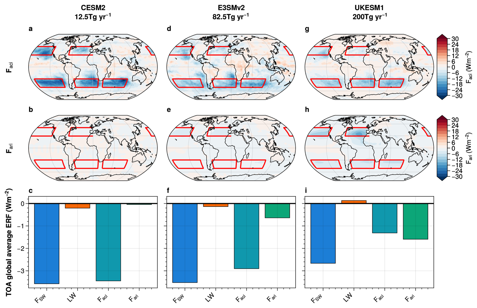
Figure 1 Spatial maps of F_aci (a, d, g) and F_ari (b, e, h), and global mean forcing components (c, f, i) from the fixed SST benchmark simulations from CESM2.1-CAM6 (a–c), E3SMv2.0 (d–f), and UKESM1.1 (g–i). F_aci and F_ari are computed using the approximate partial radiative perturbation (APRP) method. Red boxes show the latitude/longitude ranges of each emission region, which are North Pacific – NP (30 to 50° N; 190 to 120° W), North Atlantic –NA (30 to 50° N; 70° W to 0), South Pacific – SP (50 to 30° S; 170 to 90° W), South Atlantic – SA (50 to 30° S; 55° W to 15° E), and South Indian Ocean – SI (50 to 30° S; 30° E to 100° W). For CESM2.1-CAM6 and E3SMv2.0, we compute the forcing from a simulation in which we emit iSSA into each midlatitude region equally. For UKESM1, we compute the forcing using the combination of anomalies from simulations in which iSSA are emitted into each midlatitude region individually.

2.1 iSSA size distributions

We recommend all ESMs emit iSSA particles with modal dry radii of approximately 50 nm if possible. This is in the size range that produces the most efficient brightening per unit iSSA mass for the commonly used Abdul-Razzak and Ghan (ARG) activation parametrization in CESM2.1 and E3SMv2.0 (Alterskjær and Kristjánsson, 2013; Wood, 2021). However, we note that parcel modeling with more detailed cloud droplet activation calculations suggest that smaller particles would be more effective (Connolly et al., 2014; Wood, 2021). In practice, differences in SSA emission and aerosol parameterizations may limit the size distributions that can be used in different ESMs, thus iSSA emissions that are in the accumulation mode size range more generally are acceptable given known limitations to the activation rate of sub-100nm radii particles in many GCM activation schemes (Connolly et al., 2014; Ghosh et al., 2025). We note that the amount of cloud brightening depends principally on the number of iSSA particles emitted, rather than the mass, and that the mass emitted scales as r³ for dry radii r. Hence, even relatively small differences in the emitted iSSA size can result in a substantially different mass emitted and CCN increase. For example, UKESM1.1 emitted particles with r=86 nm versus r=50 nm for CESM2.1 and E3SMv2.0, resulting in a factor of (86 nm/50 nm)³ ≈ 5 × difference in particles per unit iSSA mass. As a result, much of the difference in mass emission efficiency between E3SMv2.0/CESM2.1 and UKESM1.1 is due to differences in the emitted iSSA size, rather than any fundamental physical differences. We emphasize that it is critical that all participating models carefully document the size distributions of the MCB iSSA they emit in their simulations and information about the size distribution in the atmosphere after emissions to aid in interpretation of the simulations for data users.

2.2 Emission locations and amounts

We propose that models use commonly defined emission regions for iSSA emissions following Rasch et al. (2024), rather than be based on the susceptibility of cloud fields (Chen et al., 2024b). Though this is likely less efficient (e.g., diagnosed as radiative forcing per injected aerosol mass), as iSSA may be emitted into regions with no clouds or weakly susceptible clouds, it has certain practical and scientific benefits. Firstly, it simplifies the system identification for each ESM when setting up the G6-1.5K-MCB simulations. Secondly, it produces similar patterns of forcing across ESMs so that the climate responds to similar forcing despite uncertainties in the representation of aerosol-cloud interactions. Finally, it allows clearer intercomparisons of the aerosol-cloud interaction processes for the selected regions.

The regions we have selected (NA, NP, SA, SP, SI) are based on the patch simulations conducted for H2026. This results in gaps between emission regions in the SH midlatitudes between 50 and 30° S, though because the response to midlatitude perturbations is relatively zonally symmetric (Kang et al., 2018, H2026), we assume the response will be sufficiently similar to a complete band of emissions over the SH midlatitudes. In all three models used here, the iSSA are emitted into the vertical midpoint of the lowest layer of the model and a uniform emission rate is applied for each ocean grid cell in a given region.

We suggest 100 Tg yr⁻¹ as a starting point in Inj-seasalt-midlat-SST, as it falls within the range of nominal emission rates found in Rasch et al. (2024) (250 Tg yr⁻¹ in UKESM1, 82.5 Tg yr⁻¹ in E3SMv2.0, and 12.5 Tg yr⁻¹ in CESM2.1-CAM6). The CESM2 and E3SMv2 emission rates are smaller than those used in previous GeoMIP sea salt experiments (Alterskjær et al., 2013; Ahlm et al., 2017), which all exceed 200 Tg yr⁻¹. There are two principle reasons for this. Firstly, the differences in iSSA emission size distributions, as previous models tended to use iSSA with dry radii greater than 100 nm. Secondly, the differences in process representation, as many older models do not include the dependence of autoconversion on droplet size, which is the process that produces the aerosol-cloud lifetime effect. If a given model can only emit iSSA with radii much larger than 100nm, a larger initial mass might be necessary, as we prescribe mass emission rates assuming models use similar iSSA emission size distributions. To reduce differences in forcing between hemispheres, the emissions are distributed across regions such that there is an equal mass of emissions in each hemisphere. Because two NH regions were chosen, and three SH regions, the hemispheric areal extent of emissions differs, so 25 and 16.67 Tg yr⁻¹ per region is specified for the two NH and three SH regions respectively. While it may be possible to further minimize hemispheric forcing asymmetries by rebalancing emissions according to the forcing or climate response in each hemisphere, we choose not to. In fact, we find that applying such rebalancing may complicate intercomparisons with minimal benefit because the link between the hemispheric ERF asymmetry and the response of key climate variables, such as the ITCZ location, varies across the three ESMs (H2026). We suggest −2 W m⁻² as the target ERF for Inj-seasalt-midlat as this is the approximate forcing difference between 2020–3039 and 2100 in the SSP2-4.5 scenario.

2.3 Non-linearity

When computing a nominal benchmark emission rate for the Stage 2 simulation, we propose modelers make an assumption that the ERF due to MCB scales linearly with SSA emissions based on the ERF from the Stage 1 simulation. This is principally to minimize the computational expense of the stage 1 and 2 benchmarking simulations. However, we expect that the forcing from iSSA emissions will be fundamentally non-linear as the activation rate of CCN into new cloud droplets decreases as the CDNC concentration increases. We see clear non-linearity of the iSSA forcing for subtropical MCB in CESM2.1-CAM6, E3SMv2.0, and UKESM1.1 (Rasch et al., 2024) so additional stage 1 (Inj-seasalt-midlat-SST) simulations may be necessary in some models to characterize the dependence of ERF on iSSA emissions. In the case of UKESM1, using the linear assumption resulted in a >50 % overestimation of the midlatitude iSSA emissions required to achieve −2 W m⁻², which caused excessive cooling early on in test simulations.

We also see non-linearity in the climate response. In our G6-1.5K-MCB simulations we first compute an initial guess of the emission required over the 21st century using a linear assumption of the cooling response to MCB. However, we find that in all three models this initial linear fit to the SSP2-4.5 trajectory results in excess cooling by mid-century. Interestingly, this suggests greater cooling per unit iSSA emission as the GHG warming and MCB cooling increase. Two competing effects may come into play : we expect less efficiency from the Twomey effect as more aerosols are added, but we also expect iSSA emissions to become more effective as other sources of anthropogenic aerosols decline, as is the case in the chosen SSP2-4.5 scenario. Furthermore, as emissions increase, the F_ari contribution to the MCB ERF increases due to the saturation of the Twomey effect. On top of the forcing non-linearity, the climate responses such as cloud feedbacks, sea ice changes, and ocean circulation changes may also be non-linear in the ESMs. Thus, it is difficult to anticipate to what extent linearity holds in any given model.

2.4 Cloud droplet number concentration simulations

Though many state-of-the-art ESMs represent SSA and their interaction with clouds, some have limitations that prevent implementation of the iSSA emission perturbations described above. For example, if it is not possible to add SSA in accumulation mode size ranges or SSA are not activated into cloud droplets within the models. In these cases, it may be more practical to directly perturb CDNC within the regions. CDNC perturbations have long been used to model MCB (Rasch et al., 2009; Hirasawa et al., 2023; Chen et al., 2024b) and comparisons between SSA and CDNC simulations in CESM2.1-CAM6 and E3SMv2.0 for subtropical MCB show that there are few statistically significant differences in the climate response between the two cases, if they are set up to produce similar total radiative forcing (Rasch et al., 2024). Thus, while CDNC perturbation simulations may miss some key processes, such as aerosol direct forcing and aerosol transport, they can nevertheless be used to obtain useful information about the climate response to MCB. ESM contributions for G6-1.5K-MCB have the option to use CDNC perturbations if iSSA emissions are not feasible, although it is important to recognize this method is idealized compared to iSSA and we therefore recommend the use of iSSA emissions when possible.

We propose that CDNC simulations be conducted along the same lines as the iSSA simulations, in which benchmark simulations are used to scale the perturbation in order to achieve a target forcing.

• G4SST-cdnc-midlat (Stage 1) Fixed sea surface temperature (SST) simulation with time-constant in-cloud CDNC enhancement by factor of ≈7 in the NP and NA and ≈3 in the SP, SA, and SI from the climatological background CDNC. These enhancements are estimated assuming no cloud adjustments (i.e., solely the Twomey effect) to achieve approximately −2 W m⁻² following Wood (2021):

  $$\begin{array}{}\text{(1)}& \mathrm{\Delta }F=-F_{\circ }{f}_{\mathrm{spray}}{f}_{\mathrm{low}}{\mathit{\varphi }}_{\mathrm{atm}}\mathrm{\Delta }{\mathit{\alpha }}_{\mathrm{c}}\end{array}$$

  where f_spray is the fraction of the each hemisphere that is being perturbed, f_low is the low cloud fraction in the perturbed region, F_∘ is the annual mean solar insolation in the perturbed region, ϕ_atm is an atmospheric correction factor which depends on the transmissivity and albedo of the free troposphere, and Δα_c is the aerosol-driven change in cloud albedo. Δα_c is estimated following the Twomey's formulation (Twomey, 1977) as

  $$\begin{array}{}\text{(2)}& \mathrm{\Delta }{\mathit{\alpha }}_{\mathrm{c}}={\displaystyle \frac{{\mathit{\alpha }}_{\mathrm{c}}\left(\mathrm{1}-{\mathit{\alpha }}_{\mathrm{c}}\right)\left(r_N^{\mathrm{1}/\mathrm{3}}-\mathrm{1}\right)}{\mathrm{1}+{\mathit{\alpha }}_{\mathrm{c}}\left(r_N^{\mathrm{1}/\mathrm{3}}-\mathrm{1}\right)}}\end{array}$$

  where $r_N=N_{\mathrm{d}}^{\prime }/N_{\mathrm{d}}$ is the in-cloud CDNC enhancement factor. Thus, to achieve a given target forcing, we combine these equations to calculate the enhancement factor as

  $$\begin{array}{}\text{(3)}& r_N={\left({\displaystyle \frac{\left({\mathit{\alpha }}_{\mathrm{c}}-\mathrm{1}\right)\left({\mathit{\alpha }}_{\mathrm{c}}+\mathrm{\Delta }{\mathit{\alpha }}_{\mathrm{c}}\right)}{{\mathit{\alpha }}_{\mathrm{c}}\left({\mathit{\alpha }}_{\mathrm{c}}+\mathrm{\Delta }{\mathit{\alpha }}_{\mathrm{c}}-\mathrm{1}\right)}}\right)}^{\mathrm{3}}.\end{array}$$

  Using the CESM2 climatology, for the NH we have f_spray=0.1, f_low=0.54, and ϕ_atm=0.67 and thus Δα_c=0.16. Since α_c=0.43, we compute r_N≈7. Higher enhancements are required in the NH due to these regions having a smaller total area and fewer low clouds. We recommend that the simulations be run for least at 5 years to ensure there is sufficient signal in the radiative forcing.

• G4-cdnc-midlat (Stage 2) Coupled GCM simulation with SSP2-4.5 background conditions and constant CDNC enhancement to estimate the temperature response from MCB (ΔT_MCB). We recommend that stage 2 CDNC enhancement are rescaled from stage 1 so that the MCB ERF is approximately −2 W m⁻². Since the forcing from the Twomey effect approximately scales with the ratio of the perturbed and background CDNC to the power of one-third (Wood, 2021), multiplying the enhancement factors by $\mathit{\alpha }=(-\mathrm{2}\mathrm{W}{\mathrm{m}}^{-\mathrm{2}}/{\mathrm{ERF}}_{\mathrm{stage}\mathrm{1}}{)}^{\mathrm{3}}$ may provide a reasonable guide for adjusting the forcing. We recommend that the simulations be run for at least 20 years to ensure there is sufficient signal in the global temperature response

Performing both CDNC and iSSA experiments may provide insight into which processes drive inter-model differences. Since CDNC simulations avert model differences in aerosol lifetime and activation parameterizations, comparing these simulations to iSSA simulations could help understand the role of these processes versus downstream responses such as cloud adjustments.

3 G6-1.5K-MCB experiment design

The third stage of the protocol is the G6-1.5K-MCB scenario which follows the structure of the G6-1.5K-SAI scenario (Visioni et al., 2024), with MCB in the midlatitude boxes as described above rather than SAI:

• Background Scenario: SSP2-4.5.

• Target: Decadal mean global mean surface temperature (GMST) within ±0.2K of the 2020-2039 average (chosen to be representative of 1.5 K warming above preindustrial).

• Date range: 2035–2085.

We refer readers to Visioni et al. (2024) for an extended discussion of these choices.

The method for achieving the temperature target is left to individual modelers. We expect non-linearity in the forcing and response to MCB, making it difficult to maintain the temperature target using a pre-computed emission trajectory. Algorithmic controllers or manual adjustments have been required to maintain temperature targets in past scenario simulations for both SAI (Kravitz et al., 2017) and MCB (Haywood et al., 2023; Lee et al., 2025). In the testbed simulations presented below, we use algorithmic controllers for CESM2.1-CAM6, CESM2-WACCM6, and E3SMv2.0 and manual adjustments for UKESM1.1 and found them necessary for maintaining the GMST within the target range.

4 Methods

4.1 Models

We present testbed simulations using three Coupled Model Intercomparison Project Phase 6 (CMIP6) ESMs:

• CESM2.1: The Community Earth System Model version 2.1 (Danabasoglu et al., 2020) using the Community Atmosphere Model 6 (CAM6). CAM6 is the “low-top” configuration of CESM2.1 (in contrast to the “high-top” Whole Atmosphere Community Climate Model, WACCM, used in SAI modeling) which has 32 vertical levels with a model top of ∼40 km. We use the workhorse configuration with a nominal 1° horizontal resolution finite volume grid. Aerosols are represented using the Modal Aerosol Model version 4 (Liu et al., 2016) and SSA are represented in three internally mixed modes corresponding to Aitken, accumulation, and coarse mode aerosol. Cloud microphysics are treated using the Morrison–Gettelman scheme version 2 (Gettelman and Morrison, 2015) and includes SSA activation following Abdul-Razzak and Ghan (2000) and autoconversion dependence on number concentration following Khairoutdinov and Kogan (2000), allowing the model to simulate both the cloud albedo and cloud lifetime effects. We introduce iSSA emissions by increasing the flux out of the natural SSA emission parameterization, wherein SSA in bins with dry radii of 43 and 52 nm are placed into the accumulation mode with equal number flux in each bin. The ocean model is the Parallel Ocean Program 2 (POP2), the land model is the Community Land Model 5 (CLM5), and the sea ice model is the Community Ice Model version 5 (CICE5). We also use the high-top configuration, WACCM6 Middle Atmosphere (CESM2-WACCM6-MA) (Davis et al., 2023), for one G6-1.5K-MCB ensemble member from 2035 to 2070. The physics represented in this model is largely the same as in CAM6, with the key difference being the greater representation of the upper atmosphere in WACCM6-MA. We refer to the CAM6 configuration as “CESM2.1-CAM6” and the WACCM6 configuration as “CESM2-WACCM6”.

• E3SMv2.0: Energy Exascale Earth System Model version 2.0 (Leung et al., 2020; Golaz et al., 2022). E3SM was branched from a predecessor to CESM2, and therefore shares a legacy with it in many key parameterizations and components in the atmosphere and land models. Notable differences include higher atmospheric vertical resolution (72 levels up to ∼60 km), a different dynamical core with a different grid, discretization, and resolution (spectral element with cube sphere grid of ∼100 km resolution), and different ocean and ice models (based on the Model for Prediction Across Scales – MPAS). There have also been a number of changes to parameterizations of atmospheric processes, including: (1) retuning; (2) a minimum CDNC threshold; (3) reducing the dependence of the autoconversion scheme on CDNC (Ma et al., 2022); and (4) many small but potentially important changes to parameterizations (Rasch et al., 2019; Xie et al., 2018; Golaz et al., 2022). We introduce iSSA emissions using the same method as CESM2. Thus, E3SMv2 simulates the cloud albedo and cloud lifetime effects, though the strengths of each effect tend to be lower in E3SMv2 compared to CESM2 (R2024).

• UKESM1.1: United Kingdom Earth System Model version 1.1 (Mulcahy et al., 2023). UKESM1.1 uses the Unified Model (UM) for its atmosphere, Nucleus for European Modeling of the Ocean (NEMO) for its ocean, the Los Alamos sea ice model (CICE, Ridley et al., 2018) for its sea ice, and the Joint UK Land Environment Simulator (JULES) model for its land (Williams et al., 2018; Walters et al., 2019). The UKESM1.1 baseline version of the UM model uses a N96 resolution, with a latitude–longitude grid resolution of approximately 135 km at the equator and 85 vertical levels extending to 85 km. Aerosols are represented using the Global Model of Aerosol Processes (GLOMAP) with four soluble modes (nucleation, Aitken, accumulation, coarse) and including SSA. UM represents the effect of SSA on cloud droplets and subsequently on autoconversion, and thus represents the cloud albedo and lifetime effects. The sea salt aerosol parameterization is similar to CESM2.1 and E3SMv2.0, though testing in UKESM1.1 found that larger iSSA were more effective at cooling (Haywood et al., 2023) with iSSA with dry radii of 86 nm selected for this model.

4.2 Simulations

For the testbed simulations here, we have conducted a set of midlatitude MCB simulations using emission rates derived from previous exploration using subtropical iSSA emissions (Rasch et al., 2024). The benchmark emission rates used for these models bracket the 100 Tg yr⁻¹ recommended for Inj-seasalt-midlat-SST: 12.5 Tg yr⁻¹ in CESM2.1-CAM6, 82.5 Tg yr⁻¹ in E3SMv2.0, and 200 Tg yr⁻¹ in UKESM1. The effective radiative forcing (ERF) due to midlatitude MCB from fixed SST simulations is shown in Fig. 1. For CESM2.1-CAM6 and E3SMv2.0, we used SST and emission conditions averaged for 2005–2014 and repeating annually and for UKESM we used time-evolving AMIP SST and emissions from 1979 to 1988. We diagnose the cloud (F_cld) and direct (F_aer) components of the shortwave (SW) ERF using the Approximate Partial Radiative Perturbation (APRP) method (Zelinka et al., 2023). The APRP method allows a closer approximation to the Ghan (2013) method, which provides the clearest estimate of the F_aci and F_ari.

Benchmark emissions rates successfully produce similar global mean ERFs across the three models, with −2.5 to −3.5 W m⁻² of SW forcing (Fig. 1g–i). F_tot is predominantly in the SW, with minimal longwave forcing. Notably, the forcing is almost entirely due to clouds in CESM2.1-CAM6 and E3SMv2.0 (Fig. 1a and b). In UKESM1, there are similar contributions from F_aci and F_ari, with F_ari having a slightly larger effect (Fig. 1f). This means that the midlatitude iSSA perturbations we introduce in these models have a substantial “marine cloud brightening” component rather than being mainly “marine sky brightening”. That is, we find it is not primarily driven by F_ari, in contrast to what has been reported in other models and strategies (Ahlm et al., 2017; Mahfouz et al., 2023; Haywood et al., 2023).

To estimate the temperature sensitivity to MCB, we use midlatitude MCB simulations from H2026. These simulations are similar to Inj-seasalt-midlat except that they have equal emissions in each region rather than rebalancing the emission rates to ensure equal total emission rates in each hemisphere and they use emission rates that produce F_tot greater than the −2 W m⁻² target. In CESM2.1-CAM6 and E3SMv2.0, the perturbation starts in 2015, runs for 50 and 40 years respectively, and the last 30 years are used to compute the temperature response. In UKESM1, the perturbation starts in 2035, runs for 30 years, and the last 10 years are used to compute the temperature response. We find substantial cooling in all three models (Fig. 5 in H2026) with cooling rates of $\mathrm{\Delta }{T}_{\mathrm{midlat}}=-\mathrm{0.23}$ K (Tg⁻¹ yr⁻¹)⁻¹ in CESM2.1-CAM6, $\mathrm{\Delta }{T}_{\mathrm{midlat}}=-\mathrm{0.037}$ K (Tg⁻¹ yr⁻¹)⁻¹ in E3SMv2.0, and $\mathrm{\Delta }{T}_{\mathrm{midlat}}=-\mathrm{7.5}\times {\mathrm{10}}^{-\mathrm{3}}$ K (Tg⁻¹ yr⁻¹)⁻¹ in UKESM1.

The CESM2.1-CAM6, CESM2-WACCM6, and E3SMv2.0 G6-1.5K-MCB simulations use a proportional-integral controller similar to those used in past SAI simulations (MacMartin et al., 2014; Kravitz et al., 2017; Tilmes et al., 2018; Richter et al., 2022) and in Lee et al. (2025) for MCB simulations, where MCB intervention was imposed using CDNC increases. To account for the longer response timescales in our MCB simulations compared to SAI (Kravitz et al., 2016), we adjust the parameters of the controllers such that they respond more strongly to the previous year's temperatures when computing the next year's emissions. This results in notable interannual variability in the iSSA emission timeseries (Fig. 2a and b). While we expect this to have some effect on variability in the models, because the ocean thermal response is a time integrator of these perturbations, we do not see a noticeable effect in these simulations. Discussion of the controller parameters is included in Appendix A. For the CESM2-WACCM6 simulations, we use the cooling rates from the CESM2.1-CAM6 to set up the controller. The resulting G6-1.5K-MCB simulation suggests that CAM6 and WACCM6 are sufficiently similar such that the controller can maintain temperature even when using information from CESM2.1-CAM6 in CESM2-WACCM6. Manual adjustments to the emission fluxes were made in the UKESM1.1 G6-1.5K-MCB simulations at the end of each decade to maintain the temperature target (for example, simulations using emissions based on the linear cooling per unit emissions estimates from the stage 2 simulations showed excess cooling after around 2060 so the iSSA emissions were reduced for 2065–2084). We find that both algorithmic and manual control of the iSSA emissions allow reasonable adherence to the target temperature (Fig. 2a–c) in these models. We conduct three ensemble members in CESM2.1-CAM6 and UKESM1.1 and one ensemble member in E3SMv2.0 and CESM2-WACCM6.

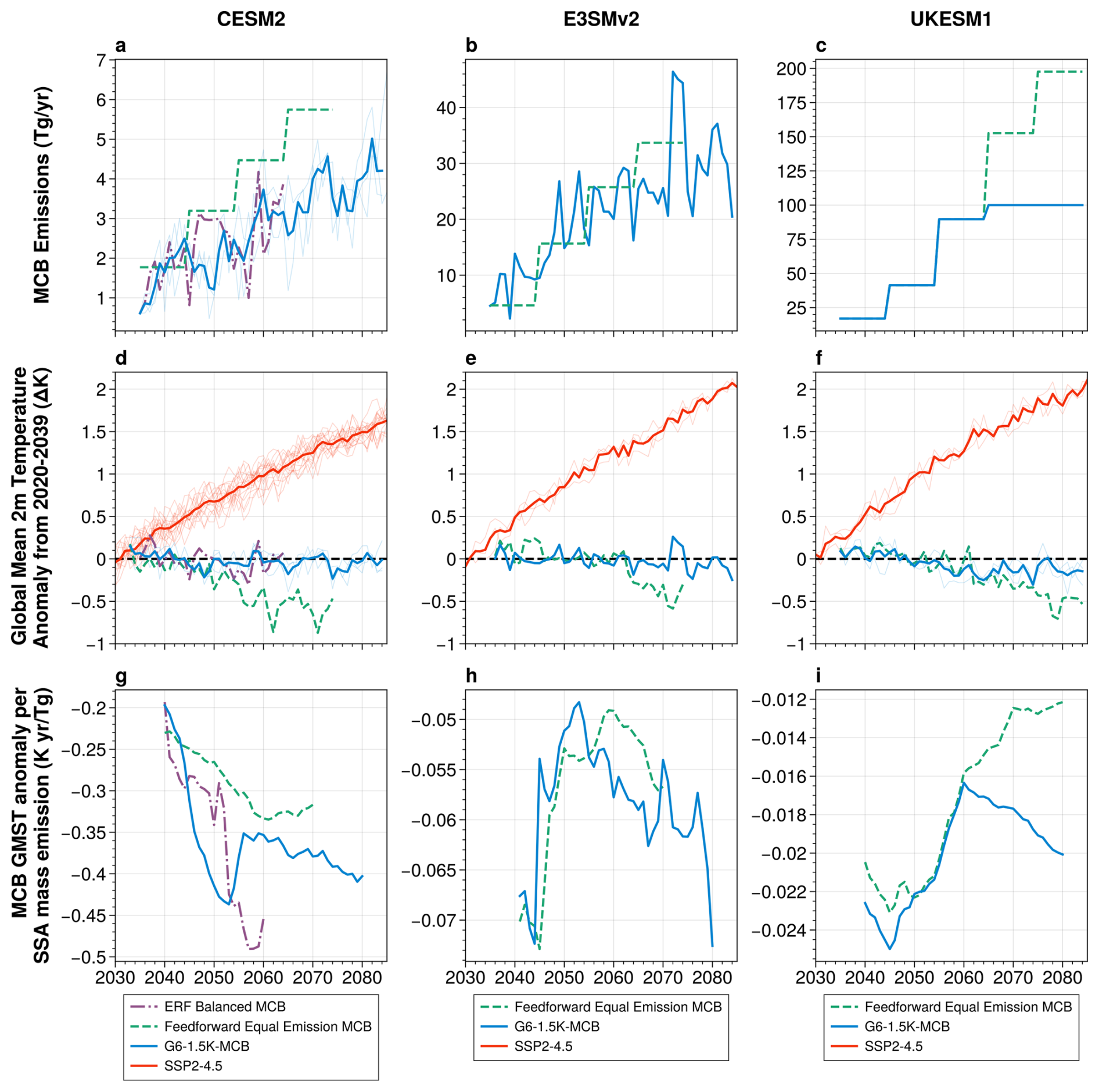
Figure 2 iSSA mass emissions (a–c), global mean surface temperature (d–f), and 10-year rolling average of GMST anomaly divided by MCB emission rate (g–i) for CESM2.1-CAM6 (a, d, g), E3SMv2.0 (b, e, h), and UKESM1.1 (c, f, i). Baseline SSP2-4.5 simulations are shown in red solid lines (thick line represents the ensemble average), G6-1.5K-MCB simulations are shown in blue solid lines, hemispheric ERF balancing simulations are shown in purple solid lines, and equal-emission feedforward simulations are shown in green dashed lines.

As a point of comparison to assess the non-linearity in the MCB forcing and response, we also include results from “feedforward” simulations. These are simulations in which the iSSA emission trajectory is computed prior to simulation using a forward estimate based on a constant, linear GMST response to mid-latitude MCB and not adjusted during the simulation (see green lines in Fig. 2a and b). For CESM2.1-CAM6 and E3SMv2.0, these simulations emitted an equal amount of iSSA into each region and for UKESM1, the simulation used mass-balanced emissions. By comparing them to the G6-1.5K-MCB simulations, we can show utility of the algorithmic and manual control of emissions and, for CESM2.1/E3SMv2.0, provide insight into the effect of redistributing the iSSA emissions to balance the hemispheric mass emissions. Finally, we also conducted a trial controller simulation in CESM2.1-CAM6 in which emissions were scaled to achieve similar ERF between hemispheres using forcing information from fixed-SST patch simulations (from H2026) but is otherwise the same as G6-1.5K-MCB. CESM2.1-CAM6 shows stronger ERF in the SH midlatitude regions compared to the NH midlatitude regions, so we use 9.9 Tg yr⁻¹ in the NH and 5.0 Tg yr⁻¹ in the SH. We use this simulation to assess the best approach to ensuring minimal shifts in tropical rainfall due to interhemispheric asymmetries in forcing or temperature response.

5 Climate response

Figure 2 shows that midlatitude MCB is able to maintain GMST to the target values, within the 0.2 K tolerance in all three models (and for CESM2-WACCM6 in Fig. B2b). Figure 2 displays the emission required to maintain GMST to the target temperature in each model (Fig. 2a–c), the resulting temperature timeseries (Fig. 2d–f), and the rolling mean GMST anomaly from SSP2-4.5 divided by the emission rate (Fig. 2g–i). We see an order of magnitude difference in the iSSA emission mass required between the models, with CESM2.1-CAM6 reaching ∼5 Tg yr⁻¹, E3SMv2.0 reaching ∼30 Tg yr⁻¹, and UKESM reaching ∼100 Tg yr⁻¹ by 2085. We note that due to the difference in emitted iSSA size distributions between UKESM1.1 and E3SMv2.0/CESM2.1, the global iSSA number flux requirements are more similar between the models with CESM2.1-CAM6 at $\sim \mathrm{8.2}\times {\mathrm{10}}^{\mathrm{19}}$ s⁻¹, E3SMv2.0 at $\sim \mathrm{4.9}\times {\mathrm{10}}^{\mathrm{20}}$ s⁻¹, and UKESM1.1 at $\sim \mathrm{5.4}\times {\mathrm{10}}^{\mathrm{20}}$ s⁻¹, though there is still over a factor of 6 difference in mass emission rates across the models, even after accounting for the size differences. The CESM2-WACCM6 emission rates are similar to CESM2.1-CAM6 up to 2070 (Fig. B2a). Owing to the idealized and differing iSSA emission distributions in the models and the difficulty that global models have simulating cloud responses to aerosols, these simulations are not suitable for estimating the iSSA mass or number emission required for actual deployment but are instead aimed at identifying and understanding the sources of inter-model differences in cloud and climate response to MCB.

For CESM2.1-CAM6, E3SMv2.0, and CESM2-WACCM6, the emission rates estimated by the algorithmic controller (blue lines) are lower than the estimate derived using a simple linear assumption (green lines in Figs. 2a, b and B2a). This implies the MCB impact on GMST is greater than expected later in the century (Fig. 2d and e). Correspondingly, we see that the feedforward response results in excess cooling after 2050 in CESM2.1-CAM6/WACCM6 and after 2060 in E3SMv2.0 (Fig. 2d and e). Similarly, for UKESM1.1 the feedforward emission estimate results in excess cooling after 2060, so in the final manually adjusted simulation the emissions are held at 100 Tg yr⁻¹ to meet the GMST target (Fig. 2c). Thus, across all three models there is increasing cooling efficiency from midlatitude MCB after the mid 21^st century (Fig. 2g–i). Considering the non-linearity in the Twomey effect means brightening efficiency will decrease as iSSA emissions increase, this suggests other nonlinearities drive this change in efficiency. Decreases in other aerosol emissions and increasing liquid water content due to precipitation suppression in the models may increase Twomey effect brightening, though in reality the magnitude and even sign of the latter effect is uncertain due to buffering by other processes such as enhanced entrainment (Hoffmann et al., 2024; Song et al., 2024). The MCB forcing and climate response have complex and uncertain interactions with changing temperatures, cloud fields, sea ice, ocean circulation etc. as GHG forcing increases (Wan et al., 2024; Sun et al., 2026). These results also differ from those of Haywood et al. (2023), who performed model iSSA experiments seeding relatively pristine stratocumulus cloud regions of the East Pacific and found a decreasing cooling per unit mass injection.

This is similar to findings from early SAI controller simulations (Kravitz et al., 2017), where it is attributed to decadal and longer timescale climate responses to SAI not captured by the short 10-year system identification simulations used in that study. However, in the MCB simulations shown here, the feedforward estimate is computed using the last 30 years of a 50-year simulation, meaning it is less likely that the overestimate in the iSSA in the feedforward is due to the climate not being sufficiently equilibrated in the system identification simulations. However, we note that there are slower multi-decadal to centennial timescale responses that will not be captured without even longer simulations (Kravitz et al., 2016). This suggests that non-linearities other than the timescale of response may be influencing the midlatitude MCB simulations. In contrast, more recent SAI controller simulations (ARISE-SAI – Richter et al., 2022) find that the linear assumption underestimates the emissions required throughout the 21st century. Recent MCB controller work, which modified the areal extent of CDNC perturbations (Lee et al., 2025), found that the linear assumption failed early in the simulation but was a reasonable estimate in the late 21st century. These diverging behaviours demonstrate the need for algorithmic controllers or manual re-adjustments, as it can be difficult to anticipate the direction and magnitude of non-linearities in the response prior to conducting the simulations.

The MCB cooling results in global mean precipitation reductions which exceed the increase from GHG, resulting in a net decrease across all three models (Fig. 3a–c, CESM2-WACCM6 in Fig. B2c). This corresponds to similar findings for anthropogenic sulphate aerosols and SAI, and is related to the weaker global mean precipitation increase due to longwave forcing from GHG versus precipitation decrease due to shortwave forcing from aerosols (Bala et al., 2008; Andrews et al., 2009; Irvine et al., 2019). The drying is largest in UKESM1, which has an anomaly of −0.05 mm d⁻¹ relative to the reference period while CESM2.1-CAM6 and E3SMv2.0 have anomalies of −0.03 and −0.02 mm d⁻¹ respectively. This may be because UKESM1.1 cools slightly below the target later in the century, resulting in a greater net global mean precipitation change.

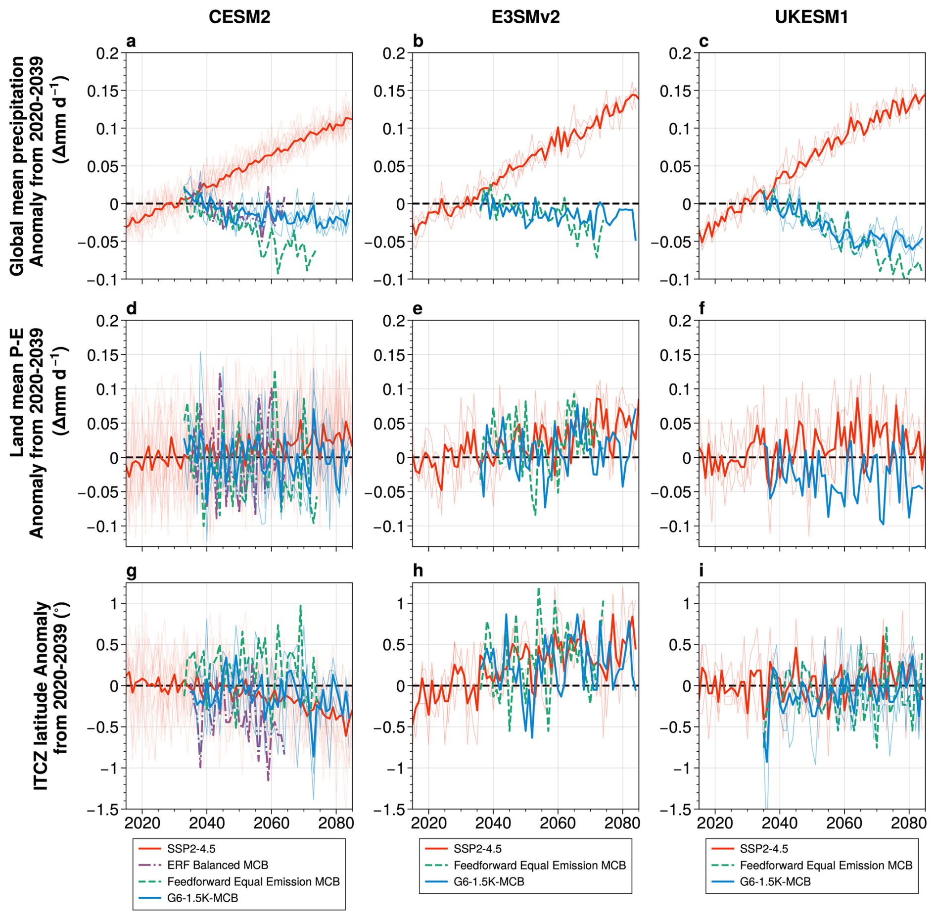
Figure 3 Annual mean global mean precipitation (a–c), land mean precipitation minus evaporation (d–f), and ITCZ latitude (g–i) anomalies for CESM2.1-CAM6 (a, d, g), E3SMv2.0 (b, e, h), and UKESM1.1 (c, f, i). Baseline SSP2-4.5 simulations are shown in red solid lines (thick line represents the ensemble average), G6-1.5K-MCB simulations are shown in blue solid lines, hemispheric ERF balancing simulations are shown in purple solid lines, and equal-emission feedforward simulations are shown in green dashed lines. The UKESM1 feedforward simulation is omitted for P−E (panel f) due to data availability.

Despite the net decrease in global precipitation, CESM2.1-CAM6, CESM2-WACCM6, and E3SMv2.0 show no change in land mean precipitation minus evaporation (P−E) (Fig. 3d and e CESM2-WACCM6 in Fig. B2d) for G6-1.5K-MCB relative to the reference period. UKESM1.1 shows a modest decrease in land P−E, though it is a smaller decrease than the global mean (Fig. 3f). Previous analysis of ocean albedo change simulations suggest that shortwave cooling over oceans results in differences in ocean versus land energy budgets that may induce circulation changes which shift precipitation from oceans onto land (Bala et al., 2011). This appears to be the case for our MCB simulations as well, and the global mean decrease is a combination of this neutral land precipitation with a larger ocean precipitation decrease. This may be a point of divergence from SAI, which causes forcing over both land and ocean. When we compute the land mean precipitation alone, we see that simulations in all three models indicate there is little change.

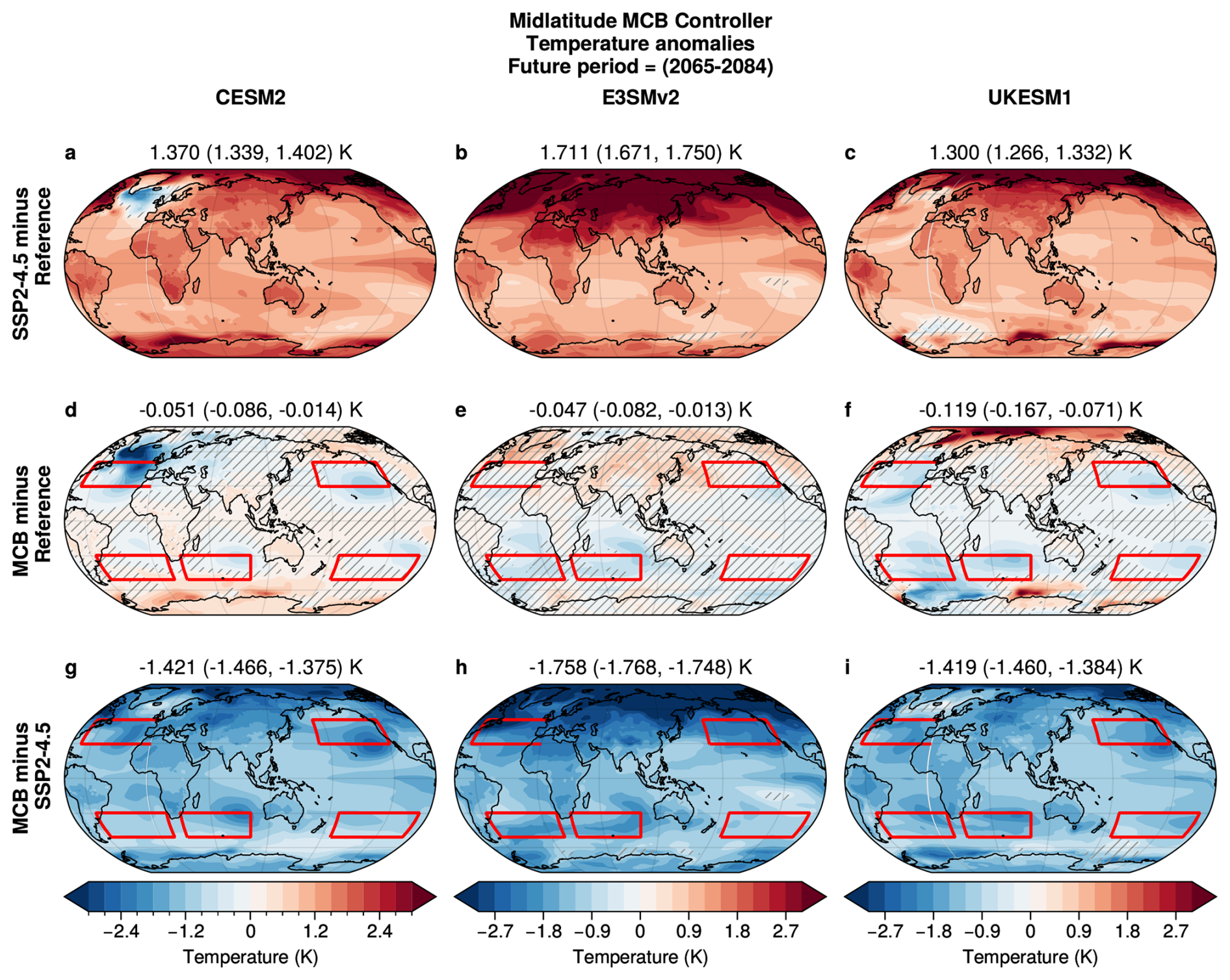
Figure 4 Annual mean temperature anomaly maps for SSP2-4.5 2065–2084 minus 2020–2039 (a–c), G6-1.5K-MCB 2065–2084 minus SSP2-4.5 2020–2039 (d–f), and G6-1.5K-MCB 2065–2084 minus SSP2-4.5 2065–2084 (g–i) for CESM2.1-CAM6 (a, d, g), E3SMv2.0 (b, e, h), and UKESM1.1 (c, f, i). Hatching indicates grid points that are insignificant at the p<0.05 level using a Student's t test. MCB iSSA emission regions are shown in red boxes.

Differences in forcing across hemispheres tend to induce shifts in tropical precipitation towards the hemisphere with greater net radiative flux due to the tendency of the intertropical convergence zone (ITCZ) to follow the energy flux equator, the latitude at which column-integrated energy fluxes go to zero (Kang et al., 2008; Kang and Xie, 2014). We compute the ITCZ latitude as the latitude of the precipitation median ϕ_median between ϕ₁=20° S and ϕ₂=20° N (Adam et al., 2016), which is the latitude ϕ_median such that

$$\begin{array}{}\text{(4)}& \underset{{\mathit{\varphi }}_{\mathrm{1}}}{\overset{{\mathit{\varphi }}_{\mathrm{median}}}{\int }}\cos \left(\mathit{\varphi }\right)P\mathrm{d}\mathit{\varphi }=\underset{{\mathit{\varphi }}_{\mathrm{median}}}{\overset{{\mathit{\varphi }}_{\mathrm{2}}}{\int }}\cos \left(\mathit{\varphi }\right)P\mathrm{d}\mathit{\varphi }\end{array}$$

for precipitation P. In CESM2.1-CAM6, SSP2-4.5 results in a southward shift of the ITCZ (Fig. 3g) while in E3SMv2.0 there is a northward shift (Fig. 3h), and in UKESM1.1 the ITCZ remains relatively stationary (Fig. 3i). The mass-balanced MCB case used in G6-1.5K-MCB has relatively little effect on the ITCZ position, relative to SSP2-4.5 in all three models. However, we do see that the ITCZ is shifted slightly northward in CESM2.1-CAM6 and southward in E3SMv2.0, offsetting the SSP2-4.5 effect. Interestingly, we see that the distribution of MCB emissions changes the ITCZ response substantially. In CESM2.1-CAM6, the ERF-balanced case shows a stronger southward shift of the ITCZ and the feedforward equal-emission simulation shows a northward shift, owing to the stronger forcing in the NH for the ERF-balanced case and in the SH for the equal emission case. This demonstrates the challenge of anticipating the tropical circulation change in the models. Not only is the response sensitive to the MCB strategy, but the models do not agree on the baseline GHG response either.

.

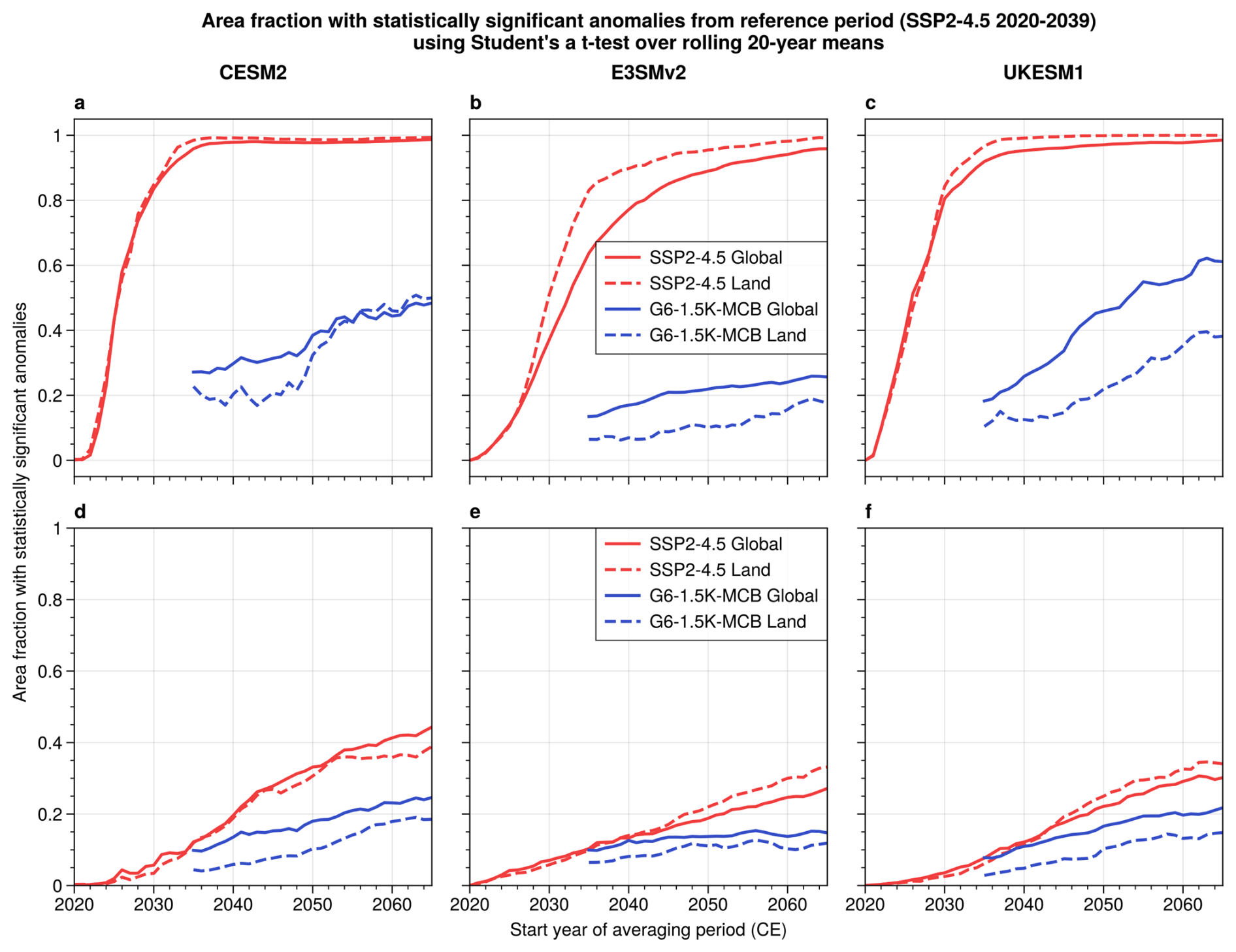
Figure 5 Time series of the area fraction with statistically significant annual mean temperature (a–c) and precipitation (d–f) anomalies for CESM2.1-CAM6 (a, d), E3SMv2.0 (b, e), and UKESM1.1 (c, f). Horizontal axis shows the start year of the 20-year averaging period used to compute the statistics. Red lines show SSP2-4.5 and blue lines show G6-1.5K-MCB. Solid lines show global area fraction and dashed lines show land area fraction.

We evaluate the pattern of climate response by comparing anomalies of the SSP2-4.5 and G6-1.5K-MCB simulations in 2065–2084 (last 20 years of the simulations) relative to the reference period (2020–2039) for each model. We can then compute the net effect of MCB as the difference between the 2065–2084 averages for G6-1.5K-MCB minus SSP2-4.5. Annual mean temperature anomaly patterns are similar across the models for SSP2-4.5 (Fig. 4a–c), with Arctic and land amplification signals characteristic of the transient climate response to GHG. However, the models differ in the North Atlantic, where CESM2.1-CAM6 sees a notable “warming hole”, UKESM1.1 sees a minimum in the warming, and E3SMv2.0 sees strong warming. This is consistent with a decline in the Atlantic Meridional Overturning Circulation in both CESM2.1-CAM6 and UKESM1, and no decline in E3SMv2.0 (Henry et al., 2025). Furthermore, E3SMv2.0 and UKESM1 warm by ≈1.7  K, compared to 1.4 K in CESM2.1-CAM6 between 2020–2039 and 2065–2084. CESM2-WACCM6 shows anomaly patterns that are very similar to CESM2.1-CAM6 and we do not discuss it further here (Fig. B1).

The G6-1.5K-MCB simulations show substantially reduced temperature anomalies (Fig. 4d–f). All three models show small (≈0.1 K) net cooling relative to the reference period, indicating that MCB emissions have successfully brought the global-mean temperature to within 0.2 K of the target. Temperatures are reduced relative to the SSP2-4.5 case in all regions and in all models (Fig. 4g–i), indicating that midlatitude MCB would not exacerbate warming in any region. There are large regions of the globe wherein the G6-1.5K-MCB temperatures are not significantly different from the reference period, especially over land regions. In CESM2.1-CAM6, 50 % of global and 52 % of land area see insignificant temperature anomalies (Fig. 5a). In E3SMv2.0, it is 74 % of global and 82 % of land area (Fig. 5b) and in UKESM1.1 it is 39 % of global and 62 % of land area (Fig. 5c). However, we do see significant residual temperature changes in many regions. In all three models, we see over cooling in the midlatitude oceans, such as in the North Pacific and SH midlatitudes, corresponding to the regions where the MCB is applied, and under cooling in certain land regions, such as over North America.

.

Figure 6 As in Fig. 4 but for annual mean precipitation.

Other residual signals are more model dependent. In CESM2.1-CAM6, there is large cooling over the North Atlantic and Europe because midlatitude MCB does not counteract the GHG “warming hole”, but instead induces more cooling (Fig. 4d). This may be because MCB is not increasing the strength of the Atlantic Meridional Overturning circulation (AMOC) enough to offset the decrease due to GHG (not shown). CESM2.1-CAM6 also shows residual warming over Antarctica and the surrounding ocean and over South America, Southern Africa, South Asia, and Australia. This is partly related to the design of the simulation, as the excessive North Atlantic cooling will lead the controller algorithm to reduce MCB emissions and undercool other regions of the globe. In E3SMv2.0, the anomalies over the North Atlantic are consistent with the reference period and overcooling is instead highest in the South Atlantic and Indian oceans (Fig. 4e). E3SMv2.0 shows residual warming over central Asia, extending from the Middle East to Western China. In UKESM1, the simulations show excess cooling in the North Atlantic. However, as the UKESM1.1 SSP2-4.5 simulation does not see a notable warming hole, the GHG signal is not exacerbated in this case. There is a substantial residual Arctic and Siberian warming in UKESM1, indicating midlatitude MCB does not fully counteract the Arctic amplification signal in this model. However, it is worth noting that in UKESM1.1 Arctic warming is 4.3±0.2 K in 2065-84 under SSP2-4.5 and 1.4±0.3 K under G6-1.5K-MCB, showing there is substantial Arctic cooling.

The simulations show there are notable inter-model differences in the G6-1.5K-MCB temperature anomalies in part because they are residuals of two fields. The effect of midlatitude MCB alone, calculated as the difference between G6-1.5K-MCB minus SSP2-4.5 (Fig. 4g–i), has an overall similar pattern across the three models, with global cooling, some Arctic Amplification, and cooling of land relative to oceans. Together this shows a MCB cooling pattern that broadly resembles the opposite of the SSP2-4.5 warming pattern, except in the southern ocean. Nevertheless, it is important to note that the models show qualitatively different regional temperature change patterns under G6-1.5K-MCB (Fig. 4d–f). This demonstrates the importance of understanding the underlying climate dynamics of the responses to SRM, how they might differ across models, and how representative these models are of the real world.

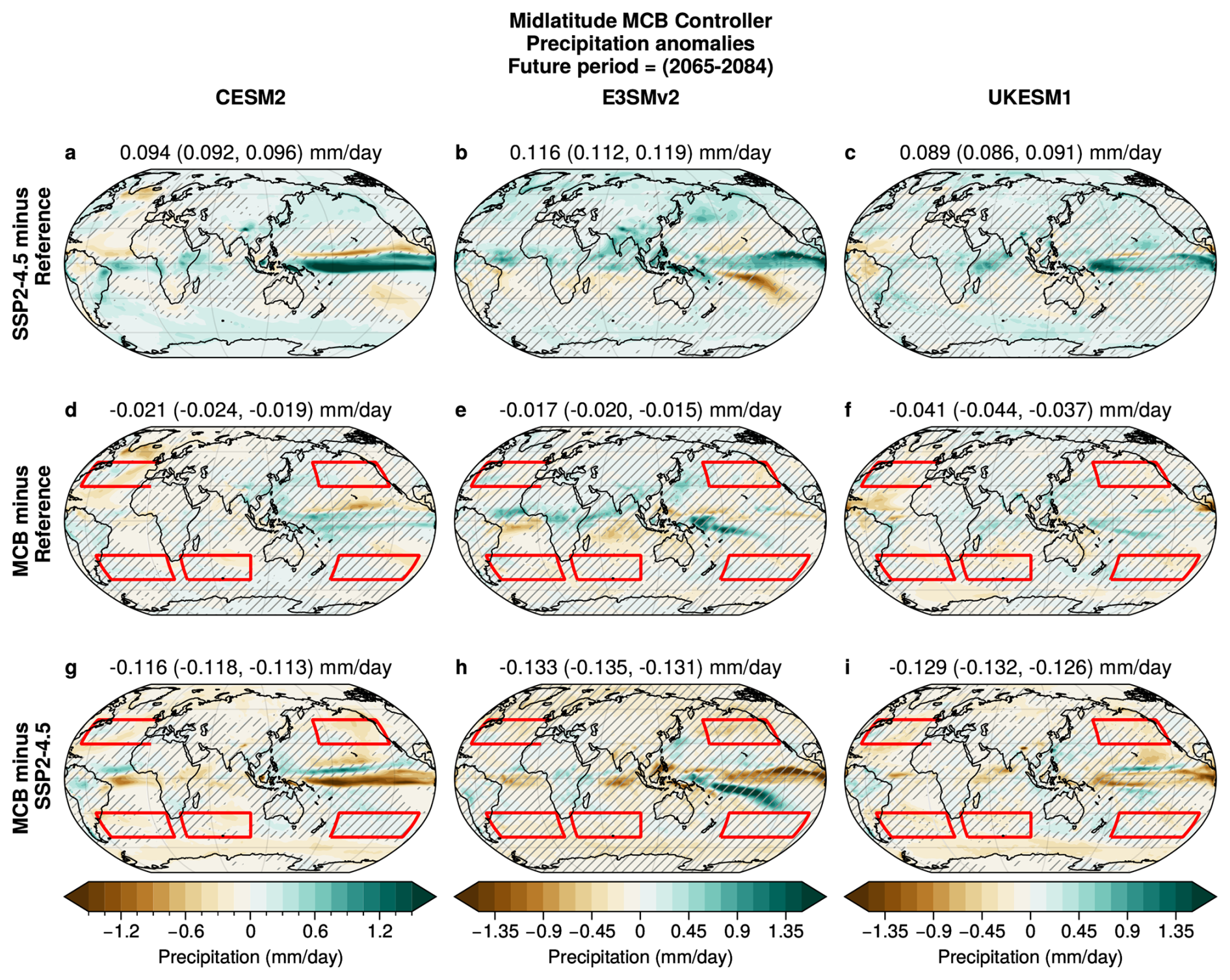
For annual mean precipitation, all three models show the characteristic GHG-driven precipitation anomaly pattern under SSP2-4.5, with increases over the tropical Pacific and Atlantic and in the mid and high latitudes along with decreases in subtropical regions (wet-get-wetter and dry-get-dryer) (Fig. 6a–c). The point-wise signal to noise is much smaller for precipitation, so differences between the models are difficult to detect at a statistically significant level. In the G6-1.5K-MCB simulations, there is a net decrease in global mean precipitation across all three models (Fig. 6d–f). However, we see that there are very few land regions with statistically significant precipitation anomalies. The main notable signal is a positive anomaly in Central Africa for E3SMv2.0. Precipitation decreases mainly occur over oceans, with significant drying anomalies in regions of the Atlantic and Pacific for all models. This means that the precipitation response to MCB is close to opposite that of SSP2-4.5 (Fig. 6g–i), characterized by decreases over the tropics, particularly the tropical Pacific, and mid/high latitudes along with increase in subtropical regions.

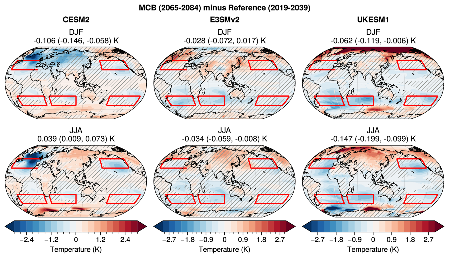
Figure 7 Seasonal mean temperature anomaly maps for G6-1.5K-MCB 2065–2084 minus SSP2-4.5 2020–2039 for CESM2.1-CAM6 (left panels), E3SMv2.0 (middle column panels), and UKESM1.1 (right column panels) for December–January–February (DJF – top row panels) and June–July–August (JJA – bottom row panels). Hatching indicates grid points that are insignificant at the p<0.05 level using a Student's t test. MCB iSSA emission regions are shown in red boxes.

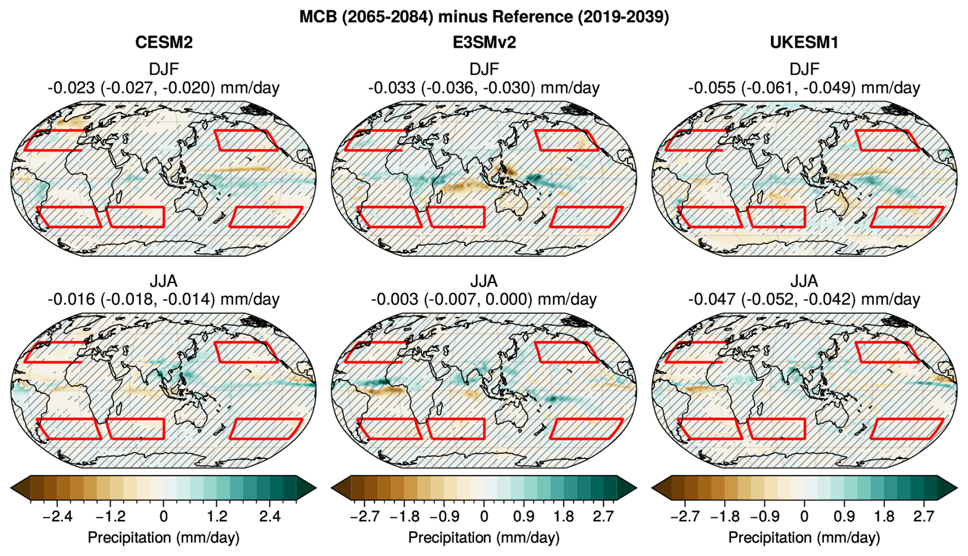
The annual mean anomalies may obscure important seasonal signals. We see that for G6-1.5K-MCB, the residual temperature anomalies differ in DJF versus JJA (Fig. 7). In all three models, there is significant residual JJA warming in Northern Eurasia and in CESM2.1-CAM6, the region shows an overcooling signal in DJF. The models also show that the under cooling over North America occurs primarily in boreal summer (JJA). The residual Arctic warming in UKESM1.1 mainly occurs in the wintertime (DJF), corresponding to the season in which Arctic amplification temperature anomalies are greatest. Seasonal precipitation maps show few significant signals over land (Fig. 8) except for E3SMv2.0 showing significant precipitation increases in central Africa in DJF and West Africa in JJA.

.

Figure 8 As in Fig. 7 but for seasonal mean precipitation.

6 Model output requested for G6-1.5K-MCB

The simulations proposed here have two primary purposes: first, to elucidate the differences across models in how clouds respond to iSSA emissions and, second, to assess the climate impacts of midlatitude MCB implementation. In addition to the core baseline CMIP7 variables (Juckes et al., 2025), we request that participating models store variables for assessing aerosol-cloud interactions. These include monthly variables requested by CFMIP, including COSP satellite simulator output and aerosol fields, and AerChemMIP, including sea salt aerosol emissions, deposition, and concentrations and aerosol number concentration (WCRP CMIP International Project Office, 2025, full lists in the aerchemmip_2d_monthly, aerchemmip_3d_monthly, CFMIP-monthly, and CFMIP-aero variable groups in the CMIP7 data request v1.2.2,)). If possible, performing additional radiation calls to compute clean-sky and clean-clear-sky fluxes following Ghan (2013) is recommended, as it enables clearer decomposition of the SW forcing into F_ari and F_aci. Furthermore, we request that modelers document information such as emitted iSSA size distribution and flux specifications and, if possible, number concentrations for sea salt aerosol and other atmospheric aerosol. This information will ensure the community can make clear comparisons between models, considering the large dependence of the MCB forcing on the size distribution of the emitted iSSA. These detailed aerosol and cloud variable outputs are highest priority for Inj-seasalt-midlat-SST, but would be of interest in the coupled G6-1.5K-MCB and Inj-seasalt-midlat simulations as well.

Priority variables for impact analysis are summarized in Visioni et al. (2024), most of which are included in the baseline CMIP7 variable lists. GeoMIP SAI data has been requested for marine and land biogeochemistry, fisheries, and agricultural assessment and modeling, so similar output would be recommended for MCB as well. Impact analysis variables are highest priority for the G6-1.5K-MCB simulations, as we anticipate this simulation will be of greatest interest for impact assessments.

7 Discussion

Recent studies have significantly advanced the understanding of how MCB is represented in ESMs and the potential climate impacts of MCB (Haywood et al., 2023; Rasch et al., 2024; Chen et al., 2024a, H2026). Assessment of the climate response in ESMs to different regional MCB perturbations has indicated that midlatitude MCB intervention can produce a cooling pattern that resembles and opposes the GHG warming pattern (H2026), in contrast to the strongly patterned cooling in response to subtropical or tropical MCB interventions that have been used in previous studies. It may therefore be thought of as a “cooperative” MCB scenario in which MCB is deployed to meet a global target, as it broadly reduces temperatures globally and produces fewer unintended regional climate changes compared to subtropical MCB. To facilitate evaluation of midlatitude MCB, and comparison of MCB versus SAI, we propose here a protocol named G6-1.5K-MCB, that uses midlatitude iSSA emissions, but is in other respects quite similar to G6-1.5K-SAI, which has already been accepted as a GeoMIP scenario.

Owing to the substantial uncertainty in the representation of aerosol-cloud interactions in ESMs and consequently the wide range in ESM radiative responses to MCB, we further define a two-stage set of benchmarking simulations (Inj-seasalt-midlat-SST and Inj-seasalt-midlat) with the aim of establishing the iSSA emission strength information needed to set up the stage 3 G6-1.5K-MCB simulations for each model. Furthermore, we request aerosol and cloud information from the fixed SST simulation to enable clear comparisons of the MCB ERF across models. These simulations use a protocol similar to past GeoMIP MCB simulations, G4cdnc and G4seasalt, which applied an idealized constant MCB perturbation in the tropics between 30° S and 30° N starting in 2015 of an RCP4.5 simulation. We include suggestions for analogous CDNC perturbation simulations, as some ESMs may not represent iSSA-cloud interactions with sufficient fidelity to conduct useful iSSA emission simulations. Though CDNC and iSSA perturbations differ, such as due to the advection of aerosol when using iSSA emissions and the partitioning between F_aci and F_ari, CESM2.1-CAM6 and E3SMv2.0 simulation results suggest that the climate response will be relatively insensitive to the perturbation method – if similar radiative forcings are used (Rasch et al., 2024). Nevertheless, modelers should use iSSA perturbations when possible.

Using three ESMs, we have conducted a set of testbed simulations in which MCB is applied in five midlatitude ocean regions (North Atlantic and Pacific; South Atlantic, Pacific, and South Indian oceans). Simulation results in all three indicate that midlatitude MCB can successfully maintain global mean temperatures close to the 2020–2039 reference period climate. In two of the three models (CESM2.1-CAM6 and E3SMv2.0), the majority of the forcing occurs via F_aci while UKESM1.1 shows similar contributions from F_ari and F_aci for a 200 Tg yr⁻¹ emission rate simulation. This is in contrast to previous work that found a predominant role for F_ari (Ahlm et al., 2017; Mahfouz et al., 2023). Ongoing CMIP6-generation model intercomparison work suggests that the MCB ERF is mainly F_aci in other current-generation ESMs as well. The models require substantially different iSSA emission rates in the G6-1.5K-MCB simulations, with a factor of 20 difference in the iSSA mass flux and a factor of 7 difference in number flux between CESM2.1-CAM6 and UKESM1.1 to maintain the temperature target. The mass emission rates used in CESM2.1-CAM6 and E3SMv2.0 simulations are lower than many previous estimates (Partanen et al., 2012; Jones and Haywood, 2012; Alterskjær et al., 2013; Ahlm et al., 2017; Haywood et al., 2023). For the 2075–2084 average, CESM2.1-CAM6 and E3SMv2.0 are lower by 53× and 8.9× respectively compared to the equivalent period in NorESM1 (266 Tg yr⁻¹) which had the lowest emission rate in Alterskjær et al. (2013). Thus, the results presented here indicate that the emissions required to produce significant cooling with MCB may be much lower than indicated in previous studies.

This has several possible explanations. First, the size distributions used here are smaller than many previous studies (Partanen et al., 2012; Jones and Haywood, 2012; Ahlm et al., 2017), except for Partanen et al. (2012) where iSSA with a dry diameter of 100 nm shows 2.1 W m⁻² with 20 Tg yr⁻¹. Second, we use a lower target than Haywood et al. (2023) which cooled from SSP5-8.5 to SSP2-4.5, requiring over 3 °C of cooling versus up to 2 °C in this scenario. Third, we use midlatitude emissions, which the three models here suggest produce stronger MCB forcing (H2026). Fourth, there have been updates in the representation of aerosol-cloud interactions, such as prognostic sea salt aerosol interactions with clouds (which was not available in two of the three models in Alterskjær et al., 2013) and influence of CDNC on autoconversion rates, which is the source of the cloud lifetime effect. We emphasize that considering the idealized iSSA emission distributions used and the uncertainty in F_aci across ESMs, these emission rates should not be treated as estimates of the iSSA mass or number emission required in an actual deployment.

In contrast to MCB strategies focused on subtropical regions, which tend to produce regional temperature changes that exacerbate GHG warming (Haywood et al., 2023; Lee et al., 2025), the simulation results indicate midlatitude MCB produces more uniform cooling and does not exacerbate GHG warming in any regions. Midlatitude MCB also produces fewer large precipitation shifts compared to subtropical MCB and the spatial extent of statistically significant annual mean precipitation anomalies is much reduced compared to SSP2-4.5. Studies of the large scale response to other midlatitude perturbations, such as ocean heat flux anomalies (Kang et al., 2018) and regional sulphate emissions (Liu et al., 2018b), suggest that the more uniform cooling seen for midlatitude MCB may also occur in other ESMs. Notable inter-model differences in the temperature response pattern can be seen in the Arctic, North Atlantic, and Southern ocean. These appear to be primarily related to differences in the circulation response to MCB, as they largely occur away from the midlatitude forcing regions. Future assessments of potential MCB deployments therefore depend critically on the continued advancement of climate dynamics research. Additional differences may arise from model variations in the susceptibility of NH versus SH regions to MCB, which could give rise to differing inter-hemispheric asymmetries in the forcing and response.

Like G6-1.5K-SAI, the MCB scenario protocol described here attempts to strike a balance between simplicity to enable standardized, inter-comparable simulations and sufficient complexity to be relevant for assessing MCB as a climate intervention strategy. This mid-latitude implementation of MCB is able to simultaneously maintain annual-average land average temperatures, precipitation, and P−E at close to baseline values. In many SAI scenarios explored to date, temperatures, and precipitation cannot simultaneously be returned to baseline values (Richter et al., 2022; Henry et al., 2024; Brody et al., 2025), though a more thorough comparison is required to understand any potential differences between the intervention methods. The scenario choices here do not represent the most optimal or realistic MCB strategy, nor should it be interpreted as being endorsed by the modeling community as a template for real-world deployment. Depending on the desired climate outcomes, further optimization of the MCB emission pattern can likely be achieved. Here, we have used global annual average temperature as a target metric in our controller and feed-forward runs. This results in regions of over- and under-cooling in the scenario simulation with midlatitude MCB and SSP2-4.5. Furthermore, there are significant inter-model differences in the pattern of temperature response to the SSP2-4.5 scenario and midlatitude MCB. Differences in the climate response to MCB in different regions suggest it may be possible to use a more complex set of targets and controllable parameters in a controller simulation that would address the regional inhomogeneity in climate warming to some extent, for example by adjusting iSSA emissions independently in different regions. Additionally, it is important to note that a significant component of the uncertainty in the climate response to MCB stems from uncertainties in the underlying climate dynamics, which also drive significant uncertainties in future climate absent MCB. On the other hand, MCB has the potential to be deployed regionally (Wan et al., 2024; Henry et al., 2025, H2026) or may be deployed in a manner closer to weather modification to reduce local heat impacts, as is proposed in the Great Barrier Reef project (Hernandez-Jaramillo et al., 2024, 2025), which will have distinct regional and global climate impacts. Both more refined controller simulations and regional MCB scenarios are important areas of research and a multi-model G6-1.5K-MCB ensemble could serve as a common reference point for other, more exploratory analyses. As the ESM community looks towards the seventh iteration of CMIP, there will be substantial updates to ESMs and changes to the emission trajectories used by the models. G6-1.5K-MCB will provide a valuable bridge between generations; providing knowledge and expertise that can be applied to define the next generation G7-1.5K-MCB scenario.

Appendix A: Controller simulations

To set up the algorithmic controller for CESM2.1-CAM6 and E3SMv2.0, we use a single-input-single-output proportional-integral control as first described in MacMartin et al. (2014). This controller method has been used extensively for SAI scenario simulations (Kravitz et al., 2016; Tilmes et al., 2018; Richter et al., 2022) and was recently used for MCB (Lee et al., 2025) to change the cloud drop number in various locations on the globe. We use a fixed pattern of iSSA emissions and modify the magnitude of the emissions once a year in January by a single multiplicative factor applied within each region, depending on the GMST of the simulation. The multiplier is computed using the equation

$$\begin{array}{}\text{(A1)}& u\left(t\right)=-k_{\mathrm{p}}T\left(t\right)-k_{\mathrm{i}}\underset{\mathrm{0}}{\overset{t}{\int }}T\left(\mathit{\tau }\right)\mathrm{d}\mathit{\tau }\end{array}$$

where u(t) is the emission rate for the next year, T(t) is the GMST, k_p and k_i are constant parameters that set the proportional and integral gains of the controller. k_p and k_i are computed following Kravitz et al. (2016) using the time series of GMST response in Inj-seasalt-midlat, wherein iSSA emissions are suddenly applied and held constant (Fig. A1) and fitting the GMST time series with

$$\begin{array}{}\text{(A2)}& y(t+D)=\mathit{\beta }\left(\mathrm{1}-e^{-t/\mathit{\tau }}\right)\end{array}$$

where D is the frequency of emission updates, β is a coefficient corresponding to the sensitivity to MCB emissions, and τ is the e-folding time of the response. We then compute

$$\begin{array}{}\text{(A3)}& {\displaystyle }& {\displaystyle }{k}_{\mathrm{i}}={\displaystyle \frac{{\mathit{\omega }}_{\mathrm{gc}}}{M_{\mathrm{gc}}\sqrt{\left(\mathrm{1}+\tan {\left({\mathrm{\Phi }}_{\mathrm{pm}}-\mathit{\pi }/\mathrm{2}-{\mathrm{\Phi }}_{\mathrm{gc}}\right)}^{\mathrm{2}}\right)}}}\text{(A4)}& {\displaystyle }& {\displaystyle }{k}_{\mathrm{p}}=k_{\mathrm{i}}/{\mathit{\omega }}_{\mathrm{gc}}\tan \left({\mathrm{\Phi }}_{\mathrm{pm}}-\mathit{\pi }/\mathrm{2}-{\mathrm{\Phi }}_{\mathrm{gc}}\right)\end{array}$$

where ω_gc is a frequency chosen based on the desired convergence time (we choose an approximately 5 year convergence time means ω_gc=0.2 rad yr⁻¹), Φ_pm is a target phase lag (Kravitz et al., 2016, we choose a phase lag of 60°, which reduces excess amplification of natural variability), $M_{\mathrm{gc}}=\left|\right|G\left(i{\mathit{\omega }}_{\mathrm{gc}}\right)\left|\right|$ the magnitude and Φ_gc=ϕ(G(iω_gc)) the phase of the system for

$$\begin{array}{}\text{(A5)}& G\left(s\right)e^{-sD}{\displaystyle \frac{\mathit{\beta }}{\mathrm{1}+s\mathit{\tau }}}.\end{array}$$

The e-folding time for midlatitude MCB is τ=7.56 years for CESM2.1-CAM6 and τ=13.5 years for E3SMv2.0 and the magnitude is $\mathit{\beta }=-\mathrm{0.2352}$ K (Tg⁻¹ yr⁻¹)⁻¹ for CESM2.1-CAM6 and $\mathit{\beta }=-\mathrm{0.0419}$ K (Tg⁻¹ yr⁻¹)⁻¹ for E3SMv2.0. For CESM2.1-CAM6, we get k_i=1.2 Tg yr⁻¹ K⁻¹ and k_p=5.2 Tg yr⁻² K⁻¹. For E3SMv2.0, we get k_i=8.79 Tg yr⁻¹ K⁻¹ and k_p=57.06 Tg yr⁻² K⁻¹. The ratio between the components is $k_{\mathrm{p}}/k_{\mathrm{i}}=\mathrm{4.33}$ year in CESM2.1-CAM6 and $k_{\mathrm{p}}/k_{\mathrm{i}}=\mathrm{6.49}$ year in E3SMv2.0, which are larger than those used for SAI simulations (typically $k_{\mathrm{p}}/k_{\mathrm{i}}\approx \mathrm{1}$). This is due to the longer response timescales to midlatitude MCB, possibly because MCB only forces over ocean, which has a higher heat capacity while SAI forces over both land and ocean. As a result, the controller requires more weighting towards the proportional term to maintain the GMST in the target convergence time and the emissions estimated from the controller have substantially greater interannual variability than in SAI simulations (Fig. A2) as the proportional term depends on the previous year's temperature. Furthermore, we see that the emissions are more variable in E3SMv2.0 compared to CESM2.1-CAM6, again due to the higher response time scales in that model. Despite the interannual variability in the emissions, there is no noticeable change in the variability in G6-1.5K-MCB relative to the reference period. Thus, we argue that the higher proportional term and more variable MCB emissions are useful for meeting the temperature target while not introducing undue changes to variability. This may be because the ocean acts to integrate the MCB forcing perturbations over time, such that the interannual MCB variability does not result in noticeable interannual impacts on climate.

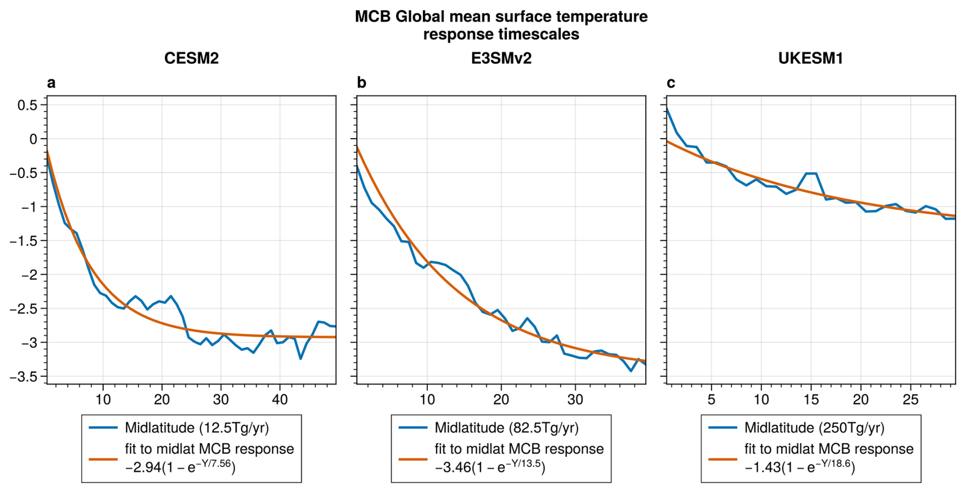
Figure A1 Annual mean GMST anomalies in Inj-seasalt-midlat from CESM2.1-CAM6 (a), E3SMv2.0 (b), and UKESM1.1 (c) with the x axis showing the years since the start of the MCB perturbation. Orange lines show a exponential fit to the GMST anomaly time series.

.

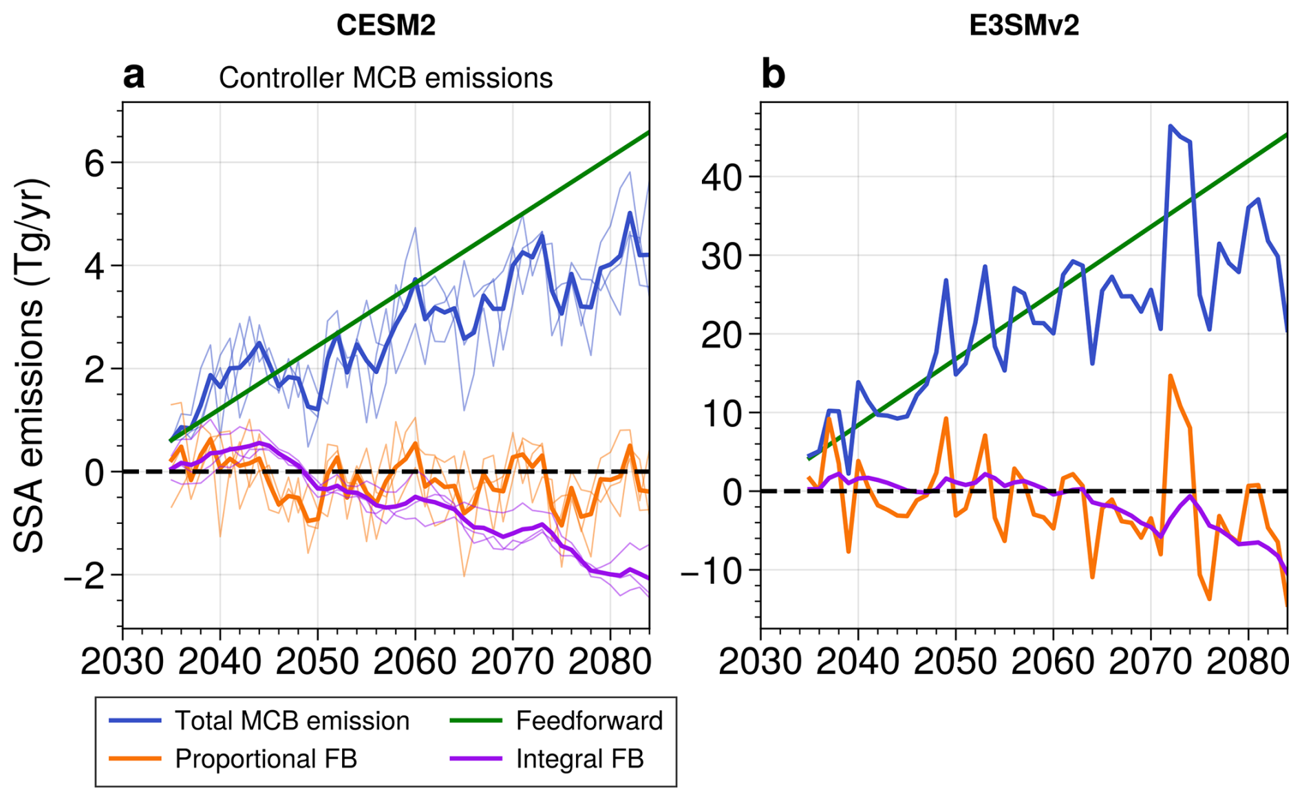
Figure A2 Algorithmic controller components from CESM2.1-CAM6 (a) and E3SMv2.0 (b). In CESM2.1-CAM6, thin lines indicate the emissions for individual ensemble members and thick lines indicate the ensemble mean. In E3SMv2.0, we have one ensemble member, so the thick lines indicate the emissions for that ensemble member.

Appendix B: Figures CESM2-WACCM6 simulations

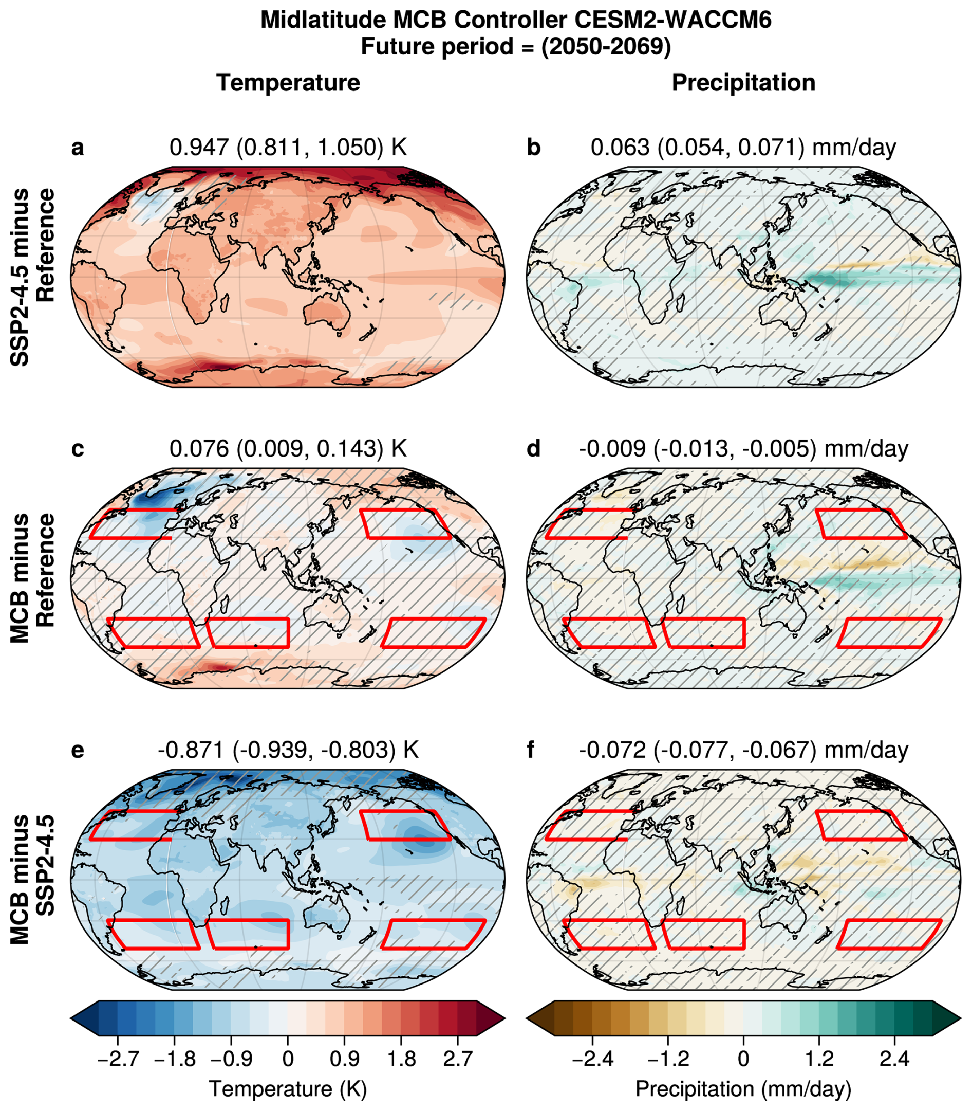
Figure B1 Annual mean temperature anomaly maps from CESM2-WACCM for SSP2-4.5 2050–2069 minus 2020–2039 (a, b), G6-1.5K-MCB 2050–2069 minus SSP2-4.5 2020–2039 (c, d), and G6-1.5K-MCB 2050–2069 minus SSP2-4.5 2050–2069 (e, f) for 2 m temperature (a, c, e) and precipitation (b, d, f). Hatching indicates grid points that are insignificant at the p<0.05 level using a Student's t test. MCB iSSA emission regions are shown in red boxes.

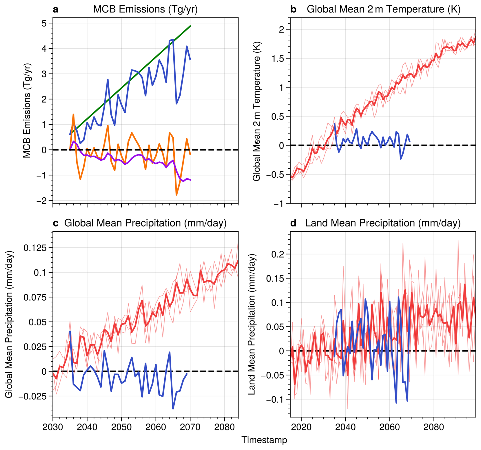
Figure B2 For CESM2-WACCM iSSA mass emissions (a), global mean surface temperature (b), global mean precipitation (c), and land mean precipitation (d). G6-1.5K-MCB simulations are shown in blue.