Modular wind profile retrieval software for heterogeneous Doppler lidar measurements (AtmoProKIT v1.1)

Retrieving wind profiles from Doppler lidar radial velocities requires processing software tools. The heterogeneity of Doppler lidar types and data acquisition settings, as well as scan patterns applied for wind profiling, makes wind profile processing challenging. Addressing this challenge, a modular open-source wind profile retrieval software tool is presented: the Atmospheric Profile Processing toolKIT (AtmoProKIT). The software calculates quality-controlled wind profiles from heterogeneous Doppler lidar data, i.e. independent of the system type, data acquisition settings, or the scan pattern applied. Ingestion of heterogeneous data is enabled by the definition of a standardized level 1 data format for the measurements, from which level 2 wind profiles are retrieved. Processing flexibility is enabled through the combination of modular processing steps in module chains. Modifications are possible by individually arranging modules, adding calculation modules, or adjusting processing parameters. The documentation of the processing steps in the result's metadata ensures the traceability of the results. A standard module chain is presented, which allows for straightforward wind profile retrieval for common Doppler lidar measurement scenarios without the need for coding. The results provided by the standard module chain are validated against radiosondes for three common Doppler lidar systems in differing atmospheric conditions. AtmoProKIT is provided as open-source Python code and includes demonstration examples, allowing easy use and future collaborative modification.

1 Introduction

Our understanding of atmospheric processes and the ability to forecast the weather rely on observations. Wind profile observations are crucial and present a missing link in the global observation system (Baker et al., 1995, 2014). Doppler lidars provide an established technique for range-resolved wind measurements using laser radiation (Werner, 2005). Using Doppler lidar measurements for model evaluation and data assimilation (Handwerker et al., 2025) requires traceable and reproducible wind profile calculations. Processing Doppler lidar measurements from multiple locations and systems (e.g. Tukiainen et al., 2024) for use in models requires flexible yet standardized calculation routines. The transformation of Doppler lidar measurements into standardized profiles must be transparent and reproducible to meet the FAIR data principles (Wilkinson et al., 2016).

Coherent Doppler lidars measure the Doppler shift of the returned laser light, scattered by aerosols or other particles, compared to the outgoing laser light. Thereby, Doppler lidars estimate the velocity of the scatterers in beam direction at different ranges along the beam. Assuming the scatterers are advected with the wind, the Doppler lidar measures the projection of the wind in beam direction, also called radial velocity. State-of-the-art Doppler lidars measure wind in a range O(100 m)–O(10 km) with high precision and accuracy.

Doppler lidars have become commercially available in the last decade and have seen increasing usage in research and industry, e.g. for atmospheric boundary layer research (Träumner et al., 2015; Adler et al., 2020) and wind energy applications (Fernando et al., 2019; Pichugina et al., 2019). Existing Doppler lidars use various laser sources (pulsed, continuous), laser pulse characteristics (e.g. wavelength, pulse energy, pulse length, pulse repetition frequency), and data processing settings (e.g. acquisition bandwidth, fast Fourier transform processing length, spectra accumulation time, number of range gates, range gate length, range gate spacing) (Werner, 2005). The ongoing development of lidar systems with different characteristics has resulted in instrument-specific heterogeneous data products and formats.

Additionally, Doppler lidars are used for a variety of application scenarios, including network wind profile retrievals (Wagner et al., 2022), turbulence estimation (Bonin et al., 2017), mixing layer height estimation (Tucker et al., 2009; Bonin et al., 2018), and multi-Doppler setups for 2D flow retrieval (Träumner et al., 2015) or virtual towers (Bell et al., 2020). The different scenarios require individual lidar and scan setups, which may additionally depend on location and time. Thereby, an additional layer of heterogeneity is introduced, since the lidar data from each application often require unique algorithms for the specific evaluation tasks.

In this study, the heterogeneity created by different systems and applications, including laser, data acquisition, and scan pattern settings, is addressed as heterogeneous Doppler lidar data.

One of the most common application scenarios for Doppler lidars is wind profiling, i.e. obtaining vertically resolved wind vector information using a single Doppler lidar (e.g. Drew et al., 2013; Baker et al., 2014; Päschke et al., 2015, and references therein). Wind profiles are easily interpretable and needed to study the atmospheric dynamics at the measurement site. Further, wind profiles can be compared to and assimilated in numerical weather prediction (NWP) models (Newsom and Banta, 2004; Kawabata et al., 2014; Pentikäinen et al., 2023).

To retrieve wind vectors (u, v, w components) from the radial velocities measured by the lidar, the lidar beam is moved through differing azimuth directions. At least three differing directions are required. One or more elevation angles are used for scans focused on wind profile retrievals. The change in the measured radial velocity with azimuth is then exploited to retrieve wind vectors using the established velocity azimuth display (VAD) (Browning and Wexler, 1968) or volume velocity processing (VVP) methods (Waldteufel and Corbin, 1978; Boccippio, 1995). By performing the retrieval at multiple distances along the beam, corresponding to multiple heights, remotely sensed vertical profiles of the wind vector (i.e. wind profiles) up to multiple kilometres in height become available (Baidar et al., 2023; Mense et al., 2024). In general, wind retrievals become more challenging under weak-signal conditions outside the planetary boundary layer (Baidar et al., 2023, and references therein).

Retrieving wind profiles from heterogeneous Doppler lidar data is not straightforward, since system setup and scan pattern vary depending on site characteristics and investigation aim (Tucker et al., 2009; Bonin et al., 2018; Pichugina et al., 2019; Steinheuer et al., 2022). Besides the system heterogeneity discussed above, a multitude of scan patterns exist for wind profiling. Trade-offs between the different scan patterns include the speed of execution, the availability of the lidar signal, or the vertical resolution. An influential parameter determined by the choice of the scan pattern is the atmospheric volume probed by the lidar. The usage of multiple consecutive scans, corresponding to temporal aggregation, is also possible in wind profile retrievals.

Both the probed volume and the aggregation time have a strong influence on retrieval accuracy due to the effect of atmospheric turbulence in the probed volume. As part of the retrieval, homogeneous flow is assumed within the volume probed by the lidar. Violations of this assumption result in retrieval error (Gasch et al., 2020), which becomes larger for shorter averaging times and scans at higher elevation angles, i.e. closer to the vertical (Rahlves et al., 2022; Robey and Lundquist, 2022). Additional factors can also induce an error in the retrieval: reasons include but are not limited to individual lidar effects and system errors (e.g. an insufficient noise compensation), range ambiguity due to high pulse repetition frequency, and the influence of local conditions (e.g. topography, blocked sectors). While wind profile retrieval from Doppler lidar data has been state-of-the-art in recent decades, it is often conducted using instrument-, setup-, or even scan-specific software (Neto and Castelao, 2023). A common methodology and processing software tool is desirable to overcome complications when processing heterogeneous lidar data from multiple systems operated in variable setups. Additionally, comparability and traceability in wind profile processing are needed, especially if heterogeneous data from multiple systems are processed, e.g. for ingestion in data assimilation for numerical weather prediction models. Examples include the processing of Doppler lidar data from network setups, currently operated in research environments (Kunz et al., 2022; Wagner et al., 2022) but likely also to be included in operational weather service networks in the near future (Kayser et al., 2021).

To our knowledge, an open-source software tool able to process a broad range of heterogeneous Doppler lidar data and provide quality-controlled wind profile retrievals is missing up to date. Based on the need for reliable wind profile retrievals from heterogeneous Doppler lidar data, the present contribution presents the Atmospheric Profile Processing toolKIT (AtmoProKIT), a new modular wind profile retrieval software. The software allows for wind profile retrievals independent of the Doppler lidar type or scan pattern used. The processing architecture is designed in a modular way and conducts a chain of concatenated processing steps, which are arranged in calculation modules. This modular architecture allows for rapid user interaction without the need for coding in the standard configuration and is open to modifications. The user can configure the processing chain according to the individual needs and extend the chain with their own algorithms. The Python code is provided to the scientific community as open-source software (https://codebase.helmholtz.cloud/KIT-KIAOS/KITcube/AtmoProKIT, last access: 2 February 2026).

The software architecture is designed to do the following:

• It handles heterogeneous data from different types of Doppler lidars with different data acquisition and scan settings without major configuration modifications. Retrieving wind profiles from heterogeneous Doppler lidar data is enabled by a common data format definition, described in Sect. 2.

• It enables wind profile retrievals in an easy-to-use and flexible way. To achieve this goal, the modular software architecture allows for easy user interaction and modification of the processing steps using so-called module chains, presented in Sect. 3.

• It provides quality-controlled and reproducible wind profile retrievals, ready for use in data assimilation and model evaluation. A standard configuration applicable to a variety of instruments and conditions is presented in Sect. 4 and validated in Sect. 5.

With its flexibility, AtmoProKIT addresses users' need for Doppler lidar measurement processing from independent data sources and gives operators an opportunity for individual settings.

2 Enabling wind profile retrievals for heterogeneous Doppler lidar data

To retrieve the 3D wind vector from Doppler lidar measurements, at least three radial velocity measurements from different, linearly independent directions are necessary. Radial velocity measurements in different directions are achieved by scanning, i.e. pointing the laser beam in differing directions. Vertically resolved wind profiles are obtained through the range-resolved measurement capabilities of lidars; i.e. the wind vector retrieval is performed at multiple altitudes using the respective radial velocity measurements.

In principle, a number of scan patterns are suitable for wind profile retrievals. Generally, the laser beam can hold a fixed position at the individual measurement positions (step-and-stare mode) or move without stopping (continuous mode). For measurements in step-and-stare mode, the laser is positioned before the measurement starts. During the measurement, the beam direction is not changed. In contrast, in the continuous mode, the beam moves during the measurements. The step-and-stare mode allows for faster movements in between measurements and, therefore, faster repeat times. Additionally, the step-and-stare mode allows for longer signal accumulation in the individual directions, increasing the availability of the lidar signal. On the other hand, continuous scans provide a better angular resolution, which can yield additional information on turbulence (Smalikho and Banakh, 2017) or the spatial variation of flow (Banta et al., 1999; Rucker et al., 2008). The continuous-scan measurements represent the wind over the angular scan sector interval.

Typical scan patterns are the following:

• step-and-stare measurements in orthogonal azimuth directions, also called Doppler beam swinging (DBS);

• arrangements of fixed-direction stares, e.g. the six-beam method (Sathe and Mann, 2013);

• azimuthal beam rotation at constant elevation, also called plan-position-indicator scans (PPIs);

• beam rotation in the elevation direction at constant azimuth, also called range–height indicator (RHI).

A common pattern for the determination of wind profiles is the PPI scan pattern, from which wind profiles can be obtained using the so-called velocity azimuth display (VAD) technique (Browning and Wexler, 1968; Päschke et al., 2015). Operators also apply other scan patterns depending on the investigation interest, which may go beyond retrieving wind profiles (Sathe and Mann, 2013; Wang et al., 2015; Smalikho and Banakh, 2017). With other patterns, interests such as a high temporal resolution (e.g. Steinheuer et al., 2022) or a high vertical resolution (RHI, PPI at low elevations) can be addressed. RHI scans allow for continuous measurements from high altitudes down to the ground, improving the vertical resolution (Rucker et al., 2008). To ensure sufficient measurements in linearly independent directions, additional measurements at differing azimuth angles are required, e.g. at least two RHI scans in differing directions. Combinations of multiple patterns or partial sector scans are also possible (Wang et al., 2015, 2016).

The common base methodology for retrieving wind vectors is a least-squares fit of the radial velocity measurements. The required calculations are presented in detail in Appendix C. The calculations minimize the radial velocities' squared deviations from the estimated wind vector, based on an assumed homogeneous wind field in the volume probed by the lidar.

2.1 Minimizing the wind vector retrieval error requires maximized data availability

The wind vector retrieval error is determined by three main factors: first, by the applicability of the homogeneous wind field assumed in the retrieval; second, by lidar measurement errors, e.g. due to random radial velocity fluctuations or beam-pointing errors; and third, by numerical errors during the calculation. If Doppler lidar measurements are compared to other instruments, sampling volume differences may introduce additional errors, which can be avoided in large-eddy-simulation-based simulator studies (Gasch et al., 2020; Rahlves et al., 2022; Robey and Lundquist, 2022; Gasch et al., 2023).

The wind vector retrieval is subject to the assumption of a homogeneous wind field inside the scan volume explored by the radial velocity measurements. Deviations from the homogeneity assumption, e.g. due to turbulence or other atmospheric variability, introduce a retrieval error even without radial velocity measurement error (Bingöl et al., 2009; Gasch et al., 2020; Rahlves et al., 2022; Robey and Lundquist, 2022). Both scan setup and aggregation time have a strong influence on retrieval error. Measurements at high elevation angles closer to the vertical result in a larger retrieval error (Teschke and Lehmann, 2017; Rahlves et al., 2022), making the inclusion of scans at low elevation angles desirable. If appropriate scan elevation angles are used, retrieval errors due to turbulence typically become negligible within a 10 min to 30 min span, depending on atmospheric conditions, but do not vanish completely (Rahlves et al., 2022; Robey and Lundquist, 2022). Therefore, a trade-off between retrieval accuracy versus temporal resolution exists.

In addition to the error introduced by the assumption of homogeneous flow, erroneous radial velocity measurements by the lidar will also introduce a retrieval error. Hence, distinguishing reliable from unreliable radial velocity measurements is a crucial challenge in the post-processing of Doppler lidar measurements. Filtering with the carrier-to-noise ratio (CNR) is a common method to improve the measurement reliability (Päschke et al., 2015; Päschke and Detring, 2024). Instead of the CNR, some instruments provide a signal-to-noise ratio (SNR) as a signal strength indicator, which can be used alternatively. In the following, only the term CNR is used. The CNR is system and measurement setup dependent and needs to be carefully characterized to determine the appropriate thresholds for reliable measurements (Pearson and Collier, 1999; Päschke and Detring, 2024). In general, stronger pulses and longer signal accumulation time (i.e. an increased number of lidar pulses) yield higher CNR. Higher CNR values provide more reliable radial velocity measurements, whereas for lower CNR the uncorrelated noise increases, making measurements less reliable (Rye and Hardesty, 1993a, b; O’Connor et al., 2010). If the CNR is too low, radial velocity measurements become random and, thus, uniformly distributed across the acquisition bandwidth in theory (i.e. white noise). In practice, suboptimal noise compensation and other effects may cause deviations from the uniform noise distribution, complicating the procedure to distinguish reliable from unreliable measurements (Manninen et al., 2016; Vakkari et al., 2019; Päschke and Detring, 2024).

For the purpose of wind profiling, on the one hand, reliable measurements may be available even at low CNR. On the other hand, measurements at high CNR may still be unreliable. Potential causes of erroneous measurements despite high CNR include second-trip echoes due to range ambiguity when using high pulse repetition frequencies (Päschke et al., 2015; Bonin et al., 2017), returns from flying objects or rain droplets, hard-target returns from terrain, and laser or data acquisition problems. As an undesired side effect of simple CNR threshold filters, many usable measurements are removed (Steinheuer et al., 2022; Päschke and Detring, 2024). Hence, more advanced filters have been introduced over time (Bonin et al., 2017; Steinheuer et al., 2022; Päschke and Detring, 2024). Advanced filter approaches aim at considering only reliable radial velocity measurements on the one hand, while ensuring broad data availability on the other hand. In some approaches, a priori information on wind field coherence based on climatology is used (Baidar et al., 2023). The trade-off between radial velocity measurement quality versus availability depends on the individual use case and may also be laser and scan pattern dependent. There is a need for a flexible implementation of various radial velocity measurement filtering approaches for different lidar systems and operation scenarios.

In principle, the least-squares fit of the radial velocities for wind vector retrieval is applicable to arbitrary scans. However, additional retrieval errors arise if the beam directions of the radial velocity measurements are not sufficiently distributed in space to ensure a reliable calculation of the resulting wind vector. In this case, the robustness and accuracy of the retrieved wind vector are not ensured (Boccippio, 1995). The condition number (CN) is a measure of the robustness of the equation system with respect to errors in the input variables (i.e. the radial velocities). In this way, an increasing CN indicates a less reliable retrieval due to a less spatially distributed beam configuration. The reason for a high CN can be imbalanced signal return from different directions or an asymmetric scan pattern. Large CNs become an issue, particularly for reduced sector scans or scans close to the vertical axis (Wang et al., 2015; Päschke et al., 2015). By considering measurements from multiple scans, the maximum available beam configuration can be utilized. Thereby, a more robust retrieval can be obtained, as long as a balanced scan is available; i.e. no direction is heavily overweighted in the measurements compared to the others.

Overall, the issues of flow homogeneity assumption violation, radial velocity reliability, and beam configuration make it desirable to utilize the maximum number of measurements available for the retrieval. A high availability of measurements reduces the uncertainty in the wind vector resulting from single random errors.

In the following, the number of measurements used for the retrieval is maximized through the definition of retrieval volumes. Within each retrieval volume, measurements are considered independent of their scan pattern origin. To enable the utilization of measurements from different scan patterns, a harmonized data format allows for ingestion of lidar data into the retrieval process independent of their origin.

2.2 Maximizing data availability through the definition of a retrieval volume

Typical scan patterns for the purpose of determining wind profiles include PPI and RHI scans or a combination of fixed-direction stares, e.g. in DBS. If the scans employ equal heights of the range gate centres (typically the case for DBS and PPI scans), the calculation of wind vectors at specific height levels can be aligned to the specific configuration. In Fig. 1, the beams on the cone represent an eight-beam step-and-stare scan with five range gates. In this scan, each range gate centre is mapped to the same height above ground for all azimuth positions. In contrast, RHI scans include elevation angle changes and thereby do not sustain the height above ground in different beams. As an example, an 18-beam RHI scan is visualized in Fig. 1. Retrieving wind vectors is not possible any more using range-gate-based retrievals.

Maximizing the data availability requires, however, the consideration of all available radial velocity measurements, independent of the scan type or range gate settings. The issue of changing absolute range gate heights has been addressed previously by studies incorporating various scan patterns (Tucker et al., 2009; Bonin et al., 2018; Pichugina et al., 2019). Similar problems arise if the lidar orientation is not stable or not aligned in a horizontal plane, as for lidars operated on ships or aircraft (Zentek et al., 2018; Gasch et al., 2023). In line with previous studies, changing absolute range gate heights are treated by binning the measurements with respect to the height above ground in this study. In this way, various lidar settings and scan patterns can be incorporated in the retrieval. Naturally, the bin size should be appropriate for the applied lidar setting and scan pattern. The bin size and spacing determine to which extent vertical gradients in the wind speed can be resolved. For very large vertical bins (several hundreds of metres), the level 1 dataset should be interpolated to the centre heights of the bins. In Fig. 1, the height bins are highlighted with the same background colour. In this way, each measured radial velocity is associated with a height bin.

In the following, the term retrieval volume describes one height bin during one temporal aggregation interval. Retrieval volumes can but need not be limited in their horizontal extent, i.e. the distance from the lidar. The definition of retrieval volumes enables the consideration of all measurements, independent of scan types or range gate settings.

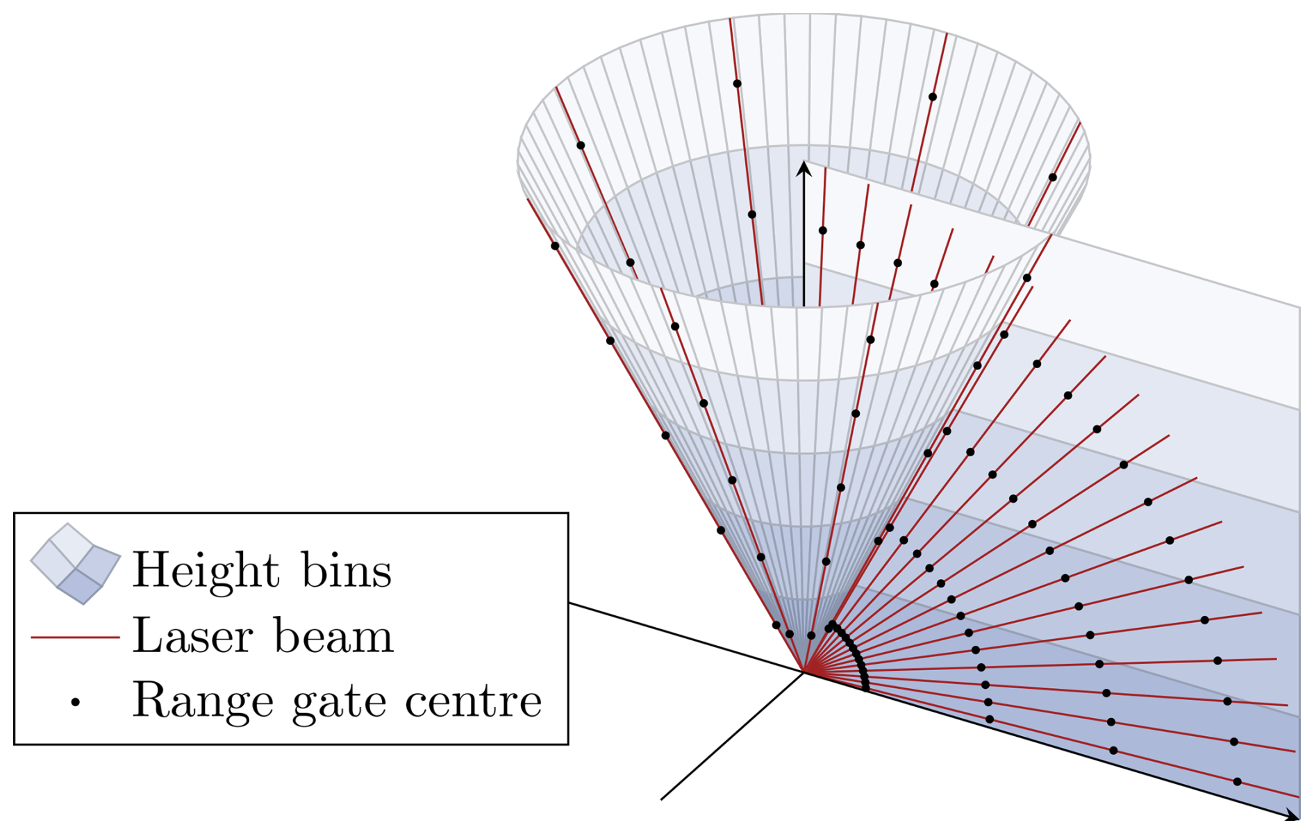
Figure 1 Visualization of typical scan patterns employed for wind profile retrieval. The respective range gate centres of all beams on the cone are mapped to the same heights, as is typical for PPI and DBS scans. In contrast, the associated height of the range gate centres in RHI scans depends on the elevation angle, which is displayed on the plane. Retrieving the wind vector based on height bins enables the consideration of all measurements within the considered time period and, therefore, maximizes the data availability.

2.3 Level 1: a harmonized data format to enable maximized data availability

Doppler lidars provide measurements in a device-specific data format (level 0). The intended applicability of the radial-velocity-based retrieval (Sect. 3) for various types of Doppler lidars and scan patterns requires a harmonized level 1 data format. A level 1 dataset supplies level 0 data for one requested instrument and a specified time span in a defined format, independent of the device-specific level 0 data format. Initially, level 0 data of the processed instrument are harmonized using a unified level 1 data structure, which serves as a common basis for the processing steps of the wind profile retrieval. The data are stored in dedicated level 1 files, each comprising the measurements of one instrument for 1 d.

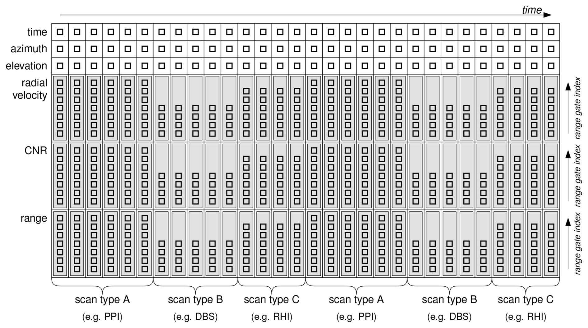
Figure 2 Level 1 format for one Doppler lidar. Using the dimensions time and range gate index enables the representation of different scan types and different settings. Scan type A could be a PPI scan with six beam positions and seven range gates, scan type B a DBS scan with four range gates, and scan type C an RHI scan with four different elevations and six range gates.

2.3.1 Level 1 data structure

The level 1 data structure incorporates the typical netCDF format introduced by Rew and Davis (1990). It is widely used for observational data at level 0, although not all instruments provide netCDF files. In netCDF, variables are specified with dependence on dimensions. Multidimensional variables are an essential part of netCDF.

Typical level 0 Doppler lidar measurements rely on the dimensions time and range. The time coordinate contains the timestamps of the measurements. The time coordinate of the level 1 dataset contains all timestamps from the respective level 0 files that are within the specified period, keeping the times provided by the instrument. The timestamp provided in the instrument-specific Doppler lidar output (level 0 files) does not necessarily present the centre of the accumulation time (e.g. for WLS200s it is the end of the accumulation time). In the case of long, non-negligible accumulation times, the timestamp should be converted when creating the level 1 dataset to represent the centre of the accumulation time. The range coordinate contains the distance of the range gate centres from the instrument. Typically, the centre of the range gate position is provided.

For each time and range, radial velocity, CNR, and possibly more measurements are provided alongside azimuth and elevation positions. Building a harmonized level 1 dataset from such level 0 datasets could be achieved by concatenating level 0 datasets along the time dimension if the range dimension remains the same. However, different range gate settings for differently configured subsequent scans (see Sect. 2.2) prevent simple concatenations of all measurements. Hence, a more general format is required.

The wind retrieval software therefore uses the dimensions time and range gate index at level 1. Using the range gate index as a dimension is independent of the real ranges, which are instead stored as a variable depending on time and range gate index. The redundancy of storing range as a function of scan type and range gate index for every time step is necessary to enable the concatenation of scans with different range gate lengths or a different number of range gates. The scan type with the highest number of range gates determines the overall size of the range gate index dimension. Unused ranges are filled with NaN in cases where a scan type uses fewer than the maximum number of range gates. Mandatory variables (associated dimensions in brackets) are time (time), azimuth (time), elevation (time), radial velocity (time, range gate index), CNR (time, range gate index), and range (time, range gate index). For scans in continuous mode, the average angles should be used. The SNR can be used instead of the CNR.

The level 1 format is not limited to the introduced variables. Further variables, such as the Doppler spectrum width (depending on time and range gate index), aerosol backscatter (depending on time and range gate index), inclination angles (depending on time), or others, can be added.

2.3.2 Exemplary representation of different scan types

Figure 2 visualizes the level 1 data format. The associated Doppler lidar conducts the scan types A, B, and C in a loop. In the time dimension, the format follows the lidar data acquisition timestamp. In the range gate index dimension, scan type A has the largest number of range gates and determines the size.

Scan type A comprises six laser beam positions and seven range gates. For each position, the corresponding timestamp, the azimuth angle, and the elevation angle are stored. The 2D variables radial velocity, CNR, and range have the shape of an array for each timestamp. Scan type B comprises only five beam positions and four range gates. Additionally, the range variable may change for different timestamps in scan type B, since the range gate length and spacing of the vertical beam are typically different for DBS. Scan type C comprises six range gates and four beam positions. While the range variable is typically constant within an RHI scan, the absolute height of each measurement has to be calculated using the variables elevation and range (see Sect. 2.2).

3 Wind profile retrieval (level 1 to level 2)

This section describes the wind profile retrieval processing. Wind vectors are calculated based on the harmonized level 1 radial velocity measurements (Sect. 2.3), which serve as input data. Level 2 data represent wind vectors per time and height aggregation bin (i.e. the wind profiles when looking at all heights), as detailed in Sect. 2.2. A new modular software architecture enables a flexible adaptation of the processing steps based on the individual conditions and user needs.

3.1 Level 2 data format

Level 2 wind vectors are represented by the wind vector direction components u, v, and w. One wind vector is calculated per bin of time and height, also termed retrieval volume. Therefore, the level 2 dimensions are time and height. Additionally, the nv dimension is used to specify the lower and upper bin bounds for both coordinates according to the CF metadata conventions (Eaton et al., 2023). Figure 3 shows a visualization of the level 2 data format. The dimensions are time, height, and nv. Besides the coordinate variables time and height, the boundary variables time_bnds and height_bnds are mandatory. The temporal and vertical resolution is specified by the user in the settings (Sect. 3.3).

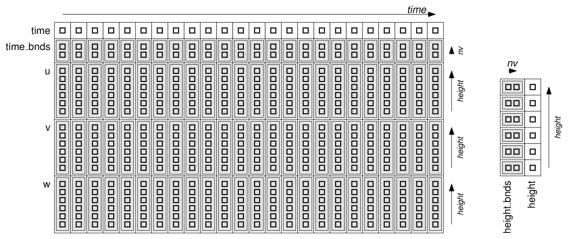
Figure 3 Level 2 format for one Doppler lidar. The coordinates are time and height. The variables u, v, and w describe the resulting wind vectors in the associated direction components.

3.2 Modular software architecture for flexible wind profile retrievals

A software architecture capable of processing measurements from various systems benefits from flexibility in the processing algorithm to adapt to individual user needs or special application cases (Sect. 1).

Hence, the software is split into modules, which each perform specific processing tasks. Each module performs a small, self-contained part of the overall processing. The desired processing of level 1 radial velocities to level 2 wind vectors is conducted through the combination of modules, which are specified in a module chain. The modular architecture enables fast reconfigurations of the processing chain, as well as extensions by other modules. New developments will be added to the code repository in the future.

3.2.1 Module chain description

The level 1 dataset (Sect. 2.3) and an empty level 2 dataset form the initial input for the module chain. Each calculation module receives both the level 1 dataset and the level 2 dataset as inputs. The calculations performed inside a module consider a set of specified variables from one or both levels. After a module's calculations are completed, the results are added as variables to the corresponding level 1/level 2 dataset or replace existing variables. Both datasets are returned, replace the originally received datasets, and serve as input for the next module in the chain. In cases where a dataset has not changed, the respective input dataset remains unchanged.

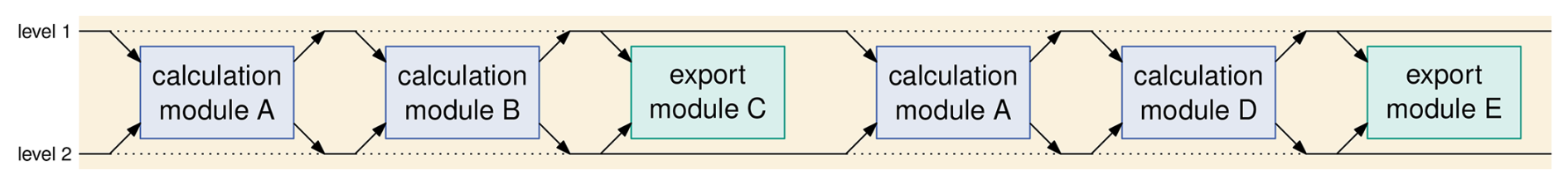
Figure 4 Schematic module chain configuration. The level 1 and the level 2 dataset can be changed by the modules according to the specified variable flow. The modules are executed sequentially and consider the calculated results of the respective predecessor module. The solid lines indicate the datasets' information flow. Datasets to be replaced are displayed with dotted lines.

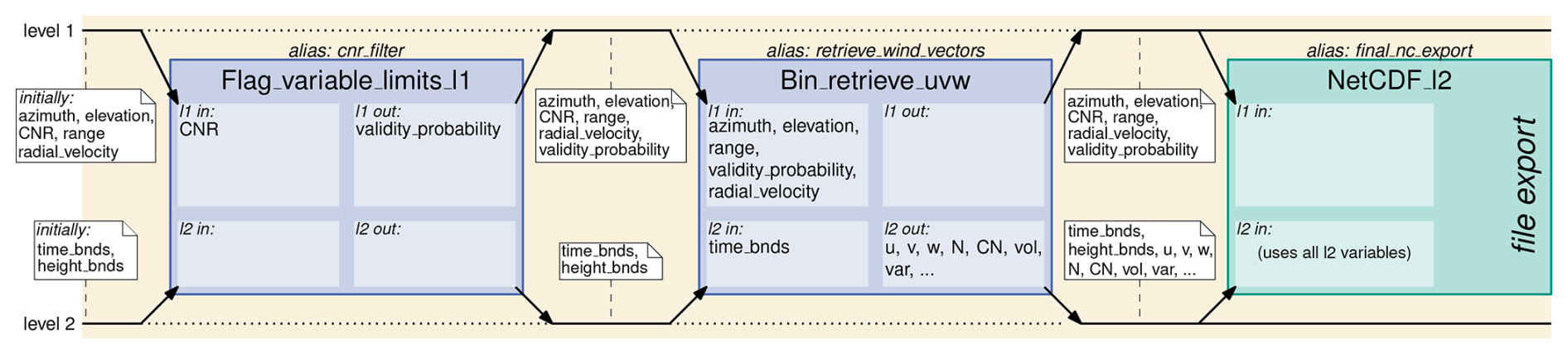
Figure 5 Exemplary module chain for a simple retrieval with CNR threshold filtering and netCDF export. For each module, considered input variables and written output variables are given by the inset boxes (l1 in, l1 out, l2 in, l2 out). The annotations outside the module boxes indicate the data contained in the level 1 and level 2 dataset. Coordinate variables (time (l1, l2), range gate index (l1), height (l2)) are not indicated.

Figure 4 shows a schematic module chain arrangement. Calculation modules include algorithms for retrieving wind vectors, indicating non-reliable measurements (e.g. based on CNR or CN values) and applying filters (e.g. level 1 data flagging of azimuth or elevation ranges), but can also include algorithms to indicate specific conditions. In addition to calculation modules, export modules can also be integrated in a module chain. Export modules export variables, e.g. as files or visualizations, but do not change the dataset itself. Required input and available output variables are specified for each module. The arrangement of the modules can follow individual needs. The modules can be arranged in an arbitrary order, as long as the necessary input variables are available in the dataset. Modules can also be used multiple times in the same module chain.

An exemplary module chain for a wind profile retrieval with a simple CNR filter is provided in Fig. 5, and the corresponding module chain file is shown in Appendix A1. The level 1 dataset initially contains the variables received from the instrument, which are CNR, range, and radial_velocity. The level 2 dataset is initially empty and contains only the level 2 bin bounds according to the selected bin specification. Coordinates (time, range gate index for level 1; time, height for level 2) describing the dataset are also contained but not visualized. Both datasets are fed into the Flag_variable_limits_l1 module, which uses the CNR variable and adds the variable validity_probability to the level 1 dataset. The validity_probability variable contains an acceptance (1.0) or rejection (0.0) value for each bin according to a user-defined threshold. The level 1 input variable CNR and the level 1 output variable validity_probability are renamings of the default variable names for the use of the Flag_variable_limits_l1 module as a CNR filter (for details, see Appendix A1).

The second module (Bin_retrieve_uvw) calculates the level 2 wind vectors based on the level 1 variables validity_probability, radial_velocity, range, azimuth, and elevation. The resulting wind vectors for each bin (u, v, w) and ancillary variables are added to the level 2 dataset. The level 1 dataset is returned without changes. Finally, the NetCDF_l2 export module writes the level 2 dataset into a netCDF file.

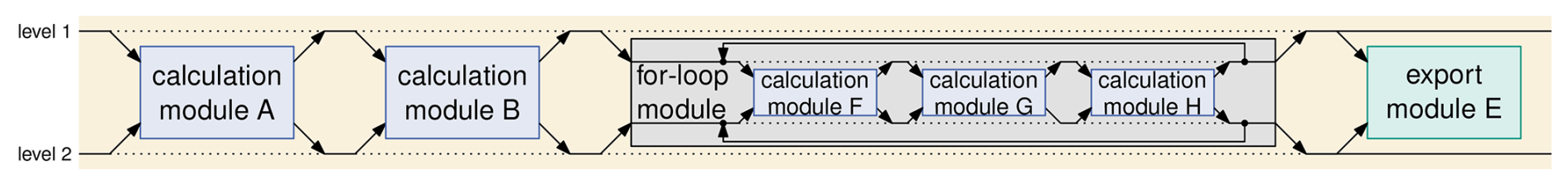
Figure 6 Module chain with a loop module. The calculation modules F, G, and H are integrated in the for-loop module which causes the repeated execution of the hierarchically integrated modules.

3.2.2 Loops in module chains

Further modules are loop modules, which enable a repetition of modules. Modules that should be repeated in a loop are hierarchically integrated in the loop modules. In Fig. 6, a for-loop module is executed after the calculation modules A and B. It contains the modules F, G, and H, which are executed multiple times in a for-loop. The number of iterations is specified in the module chain file. Additionally, a while-loop module is available, which repeats the loop as long as a condition regarding a specified level 2 variable is met. It is possible to create hierarchical configurations with loop modules within a loop module.

3.2.3 Module parametrization and variable renaming

The introduced modular retrieval configuration enables the user to arrange the calculation modules according to individual needs. Sophisticated retrievals could require an individual parametrization of the modules, depending on their position in the module chain. Therefore, an alias name has to be given to each module in a module chain. This ensures the possibility of individual module parametrization, even if the same module is contained multiple times in a module chain (see module A in Fig. 4).

Furthermore, a module arrangement can require changes to input/output variable names of modules to enable e.g. bifurcations in the processing. Renaming the default input and output variables of a module prevents the replacement of a variable by this module in the case that it is already contained in the dataset. Therefore, renaming of the variables can be specified in the module chain. This renaming and the arrangement of the modules in the module chain determine the variable flow.

3.3 Retrieval configuration

The software is executed with Python. However, for easy usability, the configuration of the module chain and settings occurs in two plain-text files. The module chain file (*.mc) contains the arrangement of the modules. The settings file (*.ini) contains the level 2 vertical and temporal resolution, directory paths, and processing parameters. A settings file for a configuration of the simple module chain (Fig. 5) is given in Appendix A2.1.

The software architecture is designed for application cases with three types of users: (1) users without programming experience with a need for straightforward Doppler lidar wind profile retrievals, (2) users with a need for detailed configurations for special circumstances or instrument conditions, and (3) methodology developers. Hence, the software architecture provides several optional configuration and extension possibilities.

1. Users with the need for straightforward Doppler lidar wind profile retrievals can resort to the standard module chain and settings for common application cases described in Sect. 4. The performance of this standard configuration is validated in Sect. 5. The user has to provide the level 1 dataset and select the instrument and the time span to be processed. The required information can be provided in an interactive dialogue or, alternatively, as command line arguments (for bash scripts). Common Doppler lidar types (WTX, WLS200s, StreamLine) are already included in the settings file; others can be added through supplying CNR acceptance thresholds for the respective device type. Except for minor adaptations such as setting import and export directories, no changes are required to the provided settings file. Instructions are given in the readme file in the code repository. An example dataset which can be processed is provided as part of this publication (https://doi.org/10.35097/xzwdzqjfyuajc0ce, Erdmann, 2025).

2. Users with the need for specific configurations can change the configuration in the module chain file and in the settings file. The JSON-formatted module chain representation allows for adding or omitting modules (see Appendix A1). Renaming the input and output variables of a module enables the user to specify the desired variable flow. By supplying module alias names, it is possible to execute the same module multiple times with individual parameter settings on each execution (see module A in Fig. 4). Detailed descriptions of the available modules and configuration instructions for users with modification purposes are available in the readme file and in the manual.

3. Developers can insert their own modules. Abstract base classes are available for calculation and export modules and ensure interoperability with the other modules. A developer has to implement the mandatory abstract methods, such as providing information on the required and generated variables. The algorithm has to be inserted in a calculation module, which receives the current level 1 and level 2 datasets as arguments. After the conduction of the algorithm, the revised level 1 and level 2 datasets have to be returned. Instructions for developers can be found in the manual.

3.4 Program execution

After the user has completed the configuration of the module chain and settings, the program can be started by executing python AtmoProKIT.py.

The selection of module chain, settings, instrument, and the time span which should be processed can be supplied by the user interactively or using a bash script. Level 1 input data are requested by the program based on the desired level 2 time span. As modules could require an extended time span to also take previous and subsequent times into consideration, the resulting required level 1 time span is calculated by requesting the required input time span for a given result time span for each module in inverse order. The corresponding method is implemented for each module and returns the required input time span for the requested time span, which is required for the successive module. Loop iterations have to be considered in the time span calculation. To avoid infinite required time spans, a maximum number of iterations has to be specified for while-loops, which is considered for the determination of the required time span. The finally resulting time span is requested from the level 1 data source. The received level 1 time span together with an empty level 2 dataset serves as initial input for the execution of the module chain. Finally, all modules are executed according to the module chain in the given order.

3.5  Tool interoperability and processing traceability

The retrieval software needs level 1 datasets as input (Sect. 2.3) and provides level 2 datasets, containing the wind profiles, as output. To ensure broad interoperability with other tools, netCDF (Rew and Davis, 1990) is supported for level 1 import and level 2 export. For easy handling within Python, xarray, introduced by Hoyer and Hamman (2017), is used as the data type to represent the level 1 and the level 2 datasets internally. Xarray uses a data representation similar to netCDF and enables simple conversion from and into netCDF and NumPy arrays. Using NumPy arrays enables significant speedup through vectorized operations (van der Walt et al., 2011). Level 1 data can be provided as netCDF files, each comprising the measurements of one instrument for 1 d. The provided level 1 files need to contain all variables required for the further processing. Through the netCDF format, pre-processing of level 1 files with other software tools is also possible. The direct integration of formats other than netCDF for level 1 import requires the implementation of an import module, which creates the required xarray dataset.

Besides tool interoperability, which is ensured through using netCDF, traceability of the processing is important. The CF conventions require an audit trail for data modifications (Eaton et al., 2023). Due to the flexibility of a module chain, adding the tool name to the metadata would not ensure sufficient traceability. Therefore, the level 2 dataset also contains the conduction history of the data-modifying calculation modules, including the parameter values. Each module execution is added, also within loops. After the netCDF export, the module chain execution history is available as an attribute in the exported netCDF file. This documentation ensures the reproducibility of the conducted processing steps.

3.6 Results of a simple module chain retrieval with CNR filtering

A simple wind profile retrieval using a fixed CNR threshold filter (module Flag_variable_limits_l1) and a common wind vector retrieval method, considering the robustness of the retrieved vectors and iteratively removing outliers (module Bin_retrieve_uvw), can be implemented in the new architecture using the module chain shown in Fig. 5. This module chain comprises the established mechanisms for wind vector retrievals and serves as a basis for further refinement in Sect. 4. Even though the Bin_retrieve_uvw module applies an iterative mechanism to remove unreliable measurements during the wind vector estimation, the initial CNR filter has the greatest influence on the data availability and quality.

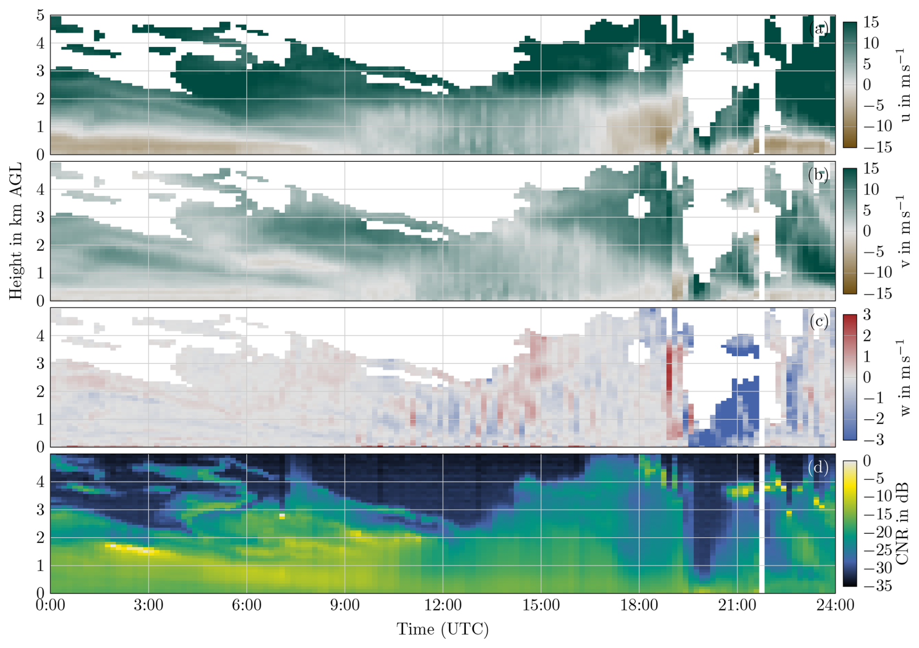
Figure 7 Wind profiles retrieved from a WLS200s Doppler lidar (a–c) and the associated median CNR per bin (d). The results are obtained using a CNR-thresholded retrieval considering radial velocity measurements with a CNR of at least −25 dB. Heavy precipitation caused a reduced range at around 20:00 UTC, and the gap at 21:40 UTC is caused by instrument failure. The retrieval is obtained from DBS and RHI scans conducted at Fischerbach (Germany) on 11 July 2023.

Figure 7a–c show the resulting wind profiles of the simple module chain exemplary for 1 d, with a bin resolution of 10 min temporally and 100 m vertically. The associated CNR levels are shown in Fig. 7d. On the one hand, the CNR threshold of −25 dB applied in this example serves as a reliable threshold for the WLS200s system used; i.e. there are no obvious retrieval outliers present. Outliers due to individual erroneous radial velocity measurements are prevented by the iterative removal of measurements with more than 3 m s⁻¹ residual in the least-squares wind vector fit of the radial velocities used in the retrieval process. On the other hand, the data availability provided by this simple wind profile retrieval is limited. The CNR values indicate a low but possibly usable signal in areas where no wind vector retrieval is available due to the conservative CNR filter applied.

Selecting a lower CNR threshold of −30 dB exploits these regions, but some of the additionally retrieved wind vectors are erroneous despite the iterative outlier removal, as indicated by outliers in the retrieved wind vectors (Fig. E1). The share of erroneous wind vectors might be acceptable for visual evaluations. However, trustworthy wind vectors are essential in the case of automated processing in subsequent evaluations or data assimilation. Hence, an extended module chain for common conditions with more sophisticated processing is introduced in Sect. 4 and validated in Sect. 5.

4 Extended standard module chain for common conditions

This section presents an extended module chain suitable for common application cases. The so-called standard module chain allows wind profile retrieval without expert methodological knowledge on the wind profile retrieval process. The standard module chain is designed to provide a high availability of retrieved level 2 wind vectors while also maintaining a high retrieval quality. The standard module chain is provided as an easy-to-use starting point for wind profile calculations (user type 1, Sect. 3.3). For specific applications or problems, the software allows for user modification, e.g. by creating specialized module chains (user types 2 and 3, Sect. 3.3).

The module chain and settings file of the standard module chain, suitable for various Doppler lidar systems and typical application cases, are provided in the code repository. The modules are arranged in the module chain configuration listed in Table 1. The corresponding variable flow is given in Table B1. This standard module chain configuration is suitable for mixtures of different scans to maximize the number of measurements used (see Sect. 2.2).

Table 1 Standard module chain for common conditions. Modules 7.1 to 7.5 are calculated in three iterations within the for-loop (module 7).

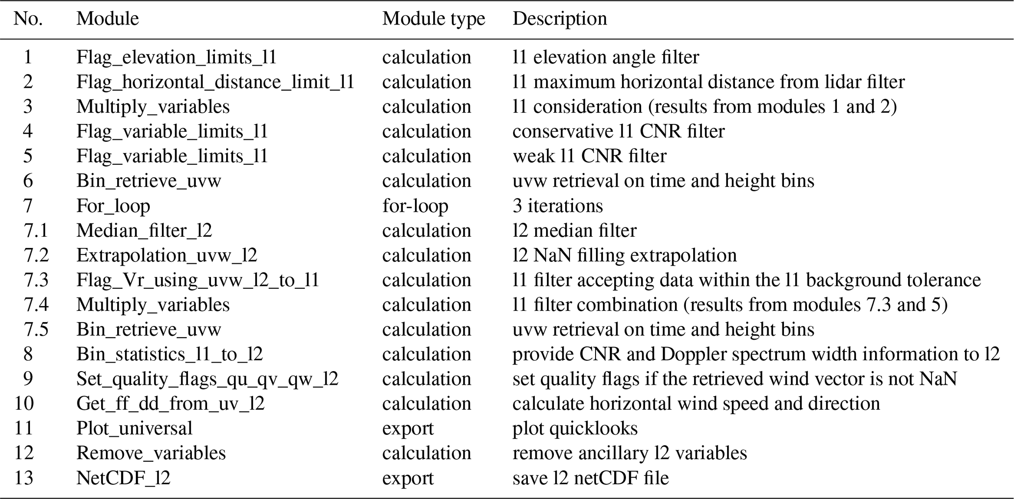
4.1 Functional description of the standard module chain

At the beginning, the standard module chain conducts an initial level 2 wind profile retrieval solely based on high-quality level 1 data, which is controlled through an initial (instrument-dependent) conservative CNR filter threshold. Despite the conservative CNR threshold, not all measurements, and thus retrievals, may be reliable (see Sect. 2). Therefore, the wind profiles resulting from the initial level 2 retrieval are further controlled using a 2D median filter, before interpolating into a so-called confidence background. Based on the filtered and interpolated level 2 confidence background, the expected level 1 radial velocity measurements are calculated. Trustworthy level 1 data with lower CNR values are then included if the radial velocity is within a maximum acceptable radial velocity deviation tolerance. Repeating the procedure in an iterative procedure refines and extends the available level 2 data. Finally, post-processing and data export are conducted.

The following paragraphs provide a description of the processing procedures and the reasoning implemented in the standard module chain. The processing parameters and thresholds contained in the modules are described. Parameters of the standard module chain, e.g. for thresholds, can be easily modified by the users in the settings file (Sect. 3.3) if needed. An overview of the default parameters used in the settings file for the standard module chain is available in Table A1.

4.1.1 Principal level 1 filtering: consideration of measurements

During the initial level 1 elevation filtering (module 1), measurements are excluded to avoid sampling biases or less robust beam constellations (see Sect. 2.1). For example, for low retrieval height bins and low elevation angles, numerous radial velocity measurements are mapped to the same height bin (see Fig. 1). Thereby, an imbalance between a high number of low-elevation (near-surface) measurements and a low number of measurements with higher elevation angles can be created. Such an imbalance negatively impacts the vertical wind velocity calculation and is, therefore, undesirable. Hence, very low scan elevations (default: below 15°) are excluded from the calculations by module 1. Module 2 limits the horizontal (not along-beam) distance for which radial velocity measurements are considered (the default value is 3 km) to reduce the impact of inhomogeneities in the far surroundings. The measurements to be considered in principle are labelled by module 3, which combines the consideration flags (0 or 1) of modules 1 and 2 by multiplication. In the further processing, level 1 measurements are only considered if the consideration flag is 1.

4.1.2 Initial wind profile retrieval and initial quality assessment

To obtain a reliable initial wind profile, a conservative CNR filter is applied in module 4. It adds a validity flag, indicating the CNR acceptance threshold is exceeded, for each level 1 measurement to the level 1 dataset. Suitable conservative CNR thresholds can vary depending on the instrument, scan setup, and environment (Päschke and Detring, 2024). A determination of suitable thresholds is possible with radial velocity vs. CNR histograms. The procedure utilized here is also explained in detail by Zentek et al. (2018).

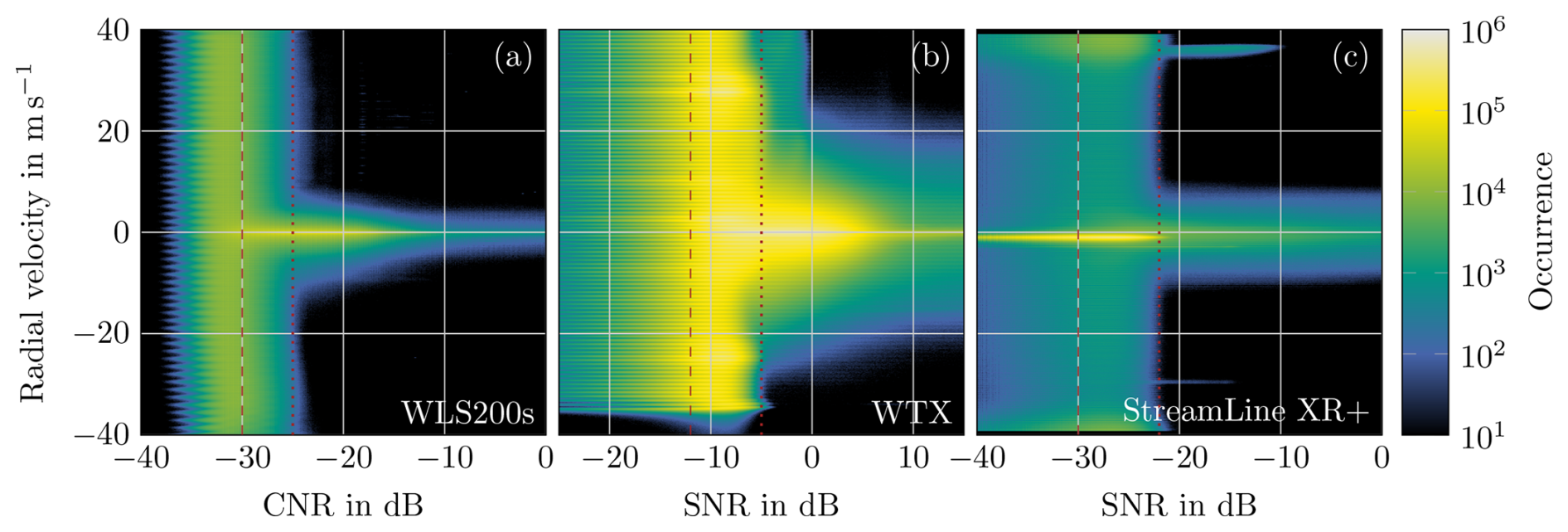
Figure 8 Occurrence of radial velocities for different CNR values for WLS200s at Payerne (a), WTX at Villingen-Schwenningen (b), and StreamLine XR+ at Neumayer Station (c). All radial velocities are summed up in bins of 0.1 dB and 0.1 m s⁻¹ between June and August 2023 for (a) and (b) and between 3 January and 26 November 2024 for (c). The selected conservative CNR thresholds are marked by dotted lines, and the weak thresholds are indicated with dashed lines.

Figure 8 shows the radial velocity vs. CNR histogram for radial velocities measured with three types of Doppler lidars. For symmetrical scans, a distribution with a peak around 0 m s⁻¹ can be expected from valid measurements. Below an instrument-specific CNR level, noise starts to occur. Noise manifests as radial velocity measurements distributed randomly across the acquisition spectrum. Thus, the histogram indicates a broadened occurrence probability for all radial velocities. The conservative CNR threshold (dotted line) should be located in a region with low random radial velocity noise and few outliers. For the WLS200s (Fig. 8a), noise begins to occur below −25 dB, indicated by the broadening of the distribution. Thus, measurements with a CNR above −25 dB are the most reliable. Therefore, the conservative default threshold for WLS200s is set to −25 dB. For the WindTracer WTX and StreamLine XR+, the conservative default thresholds are set to −5 and −22 dB, respectively.

Issues detectable in the radial velocity vs. CNR histograms can be connected to the single instrument, the settings, or local circumstances and cannot generally be attributed to the respective Doppler lidar type. For example, the peak at −1 m s⁻¹ in Fig. 8c is an unexpected issue, which is further discussed in Appendix D.

Reliable radial velocity measurements can also be available below the conservative thresholds (Päschke et al., 2015; Zentek et al., 2018; Steinheuer et al., 2022; Päschke and Detring, 2024). To mark measurements with reduced probability of validity, a second, weak CNR threshold is introduced by module 5. This lower (weak) threshold should be set in the region where radial velocities for CNR begin to appear as equally distributed. The default thresholds for this weak CNR filter are −30 dB for WLS200s and StreamLine XR+ and −12 dB for the WindTracer WTX. Users can define individual thresholds that are suitable for the noise characteristics of their instruments by configuring the retrieval (Sect. 3.3).

Wind vectors are then retrieved in module 6. The least-squares fit of the wind vector is calculated for each bin (see Appendix C) by considering the level 1 radial velocity measurements where both the consideration flag and the validity probability are 1. If level 1 measurements deviate too much from the fit, they are removed, and the wind vector calculation is repeated without them. The default accepted deviation tolerance is ±3 m s⁻¹. The retrieval procedure is repeated iteratively until all remaining measurements are within the accepted tolerance or an insufficient number remains and the wind vector is rejected.

To achieve resilient wind vectors, the retrieval quality is assessed, and the retrieved wind vector is rejected if one of the quality indicator conditions is violated. The quality indicators are the CN (default threshold: 8), the volume enclosed in the convex hull spanned by the unit vectors originating at ($\mathrm{0},\mathrm{0},\mathrm{0}$) in the laser beam directions (default threshold: 0.042, corresponding to about 2 % of the unit hemisphere explored), the absolute number of measurements (default threshold: 12), and the share of measurements that contributed to the least-squares fit (default threshold: 0.2) in relation to all considered measurements (see module 3). The CN indicates if the laser beam dispersion is sufficient (see Sect. 2.1). For unbalanced scan patterns (e.g. an overwhelming majority of vertical stares alternating with few PPI/DBS measurements), the CN may be high, yet wind profile retrieval may be possible due to the PPI/DBS measurements. The enclosed volume threshold allows for inclusion of such unbalanced scans despite a high CN. The absolute number of measurements prevents retrievals based on very few measurements, where a few erroneous measurements can have a strong influence. The relative number of measurements prevents retrievals in conditions where random noise is the dominant signal.

Up to this point, the module chain is the simple module chain (discussed in Sect. 3.6), extended by the principal level 1 filtering. The further steps improve the data basis considered for wind vector retrieval to also enable retrievals in regions with low CNR values.

4.1.3 Lower CNR acceptance threshold based on a confidence background

CNR values provide a first-order indication of data quality. However, even at low CNR, reliable measurements may be available in some circumstances, depending on atmospheric and lidar system conditions (Sect. 2.1).

To extend the availability of retrieved wind vectors at level 2, measurements with lower CNR should also be considered if they are trustworthy. Therefore, a level 2 (u, v, w) wind profile confidence background is calculated based on the initially retrieved level 2 wind profiles. Since a high reliability of the confidence background is crucial, the initially retrieved wind profiles are filtered with a median filter (default: three time bins, five height bins, i.e. depending on the selected resolution) in module 7.1 to remove potentially remaining outliers. Subsequently, the confidence background is extrapolated in module 7.2. Gaps are filled with a smooth image restoration inpainting method (https://scikit-image.org/docs/stable/api/skimage.restoration.html#skimage.restoration.inpaint_biharmonic, last access: 16 April 2025), which fills gaps seamlessly using biharmonic functions (Damelin and Hoang, 2018; Chui and Mhaskar, 2010). The weighting of time against height can be specified by the user. In the default configuration, 1 h and 1 km are weighted equally. In Fig. 9, the extrapolated confidence background is displayed for the same setting as in Fig. 7. In the default configuration, the extrapolation is limited to 1 km and 1 h.

Based on the level 2 wind profile confidence background, the expected level 1 radial velocity is calculated for every measurement. Level 1 radial velocities which are within a tolerance (default: ±3 m s⁻¹) of the radial velocity expected from the confidence background are considered (7.3), also below the conservative CNR threshold, as long as the CNR is above the weak threshold indicated by module 5. Thereby, the level 1 data basis is extended with quality-controlled radial velocity measurements exhibiting a lower CNR.

Module 7.5 performs the wind vector retrieval again but takes all measurements accepted by modules 7.3 and 5 into account. The increase in the level 1 data availability resulting from more accepted measurements results in a larger availability of retrieved wind vectors at level 2.

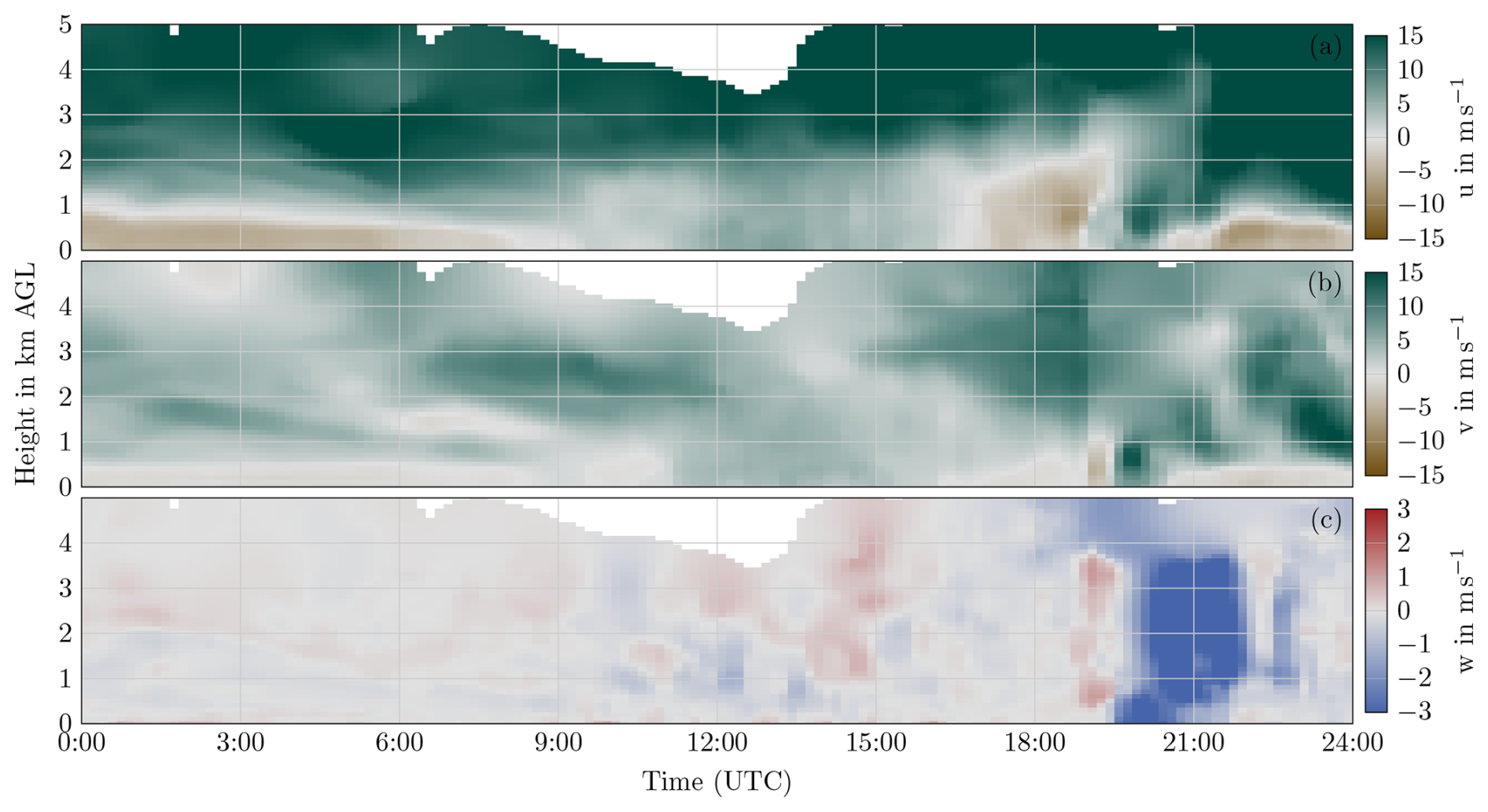
Figure 9 Wind profile confidence background. The confidence background is calculated based on the initially retrieved wind profiles using an additional median filter and subsequent extrapolation, limited to 1 km vertically and 1 h temporally. Radial velocities that deviate within a specified tolerance from the expected radial velocity according to the confidence background are considered in the next iteration if the weak CNR threshold is met.

Figure 10 Final wind profiles. All measurements with a CNR of at least −30 dB are also considered if the radial velocities deviate from the radial velocity expected from the confidence background within a range of ±3 m s⁻¹. The data availability is improved compared to the initially retrieved wind profiles, particularly in gaps.

4.1.4 Confidence background quality control

A reliable estimation of the confidence background is crucial, since it determines the acceptable radial velocity range during subsequent iterations. While the iterations allow for improvement and refinement of the confidence background, the quality of the radial velocities and of the retrieved wind vector must be ensured in every iteration. As such, accepting noisy radial velocity measurements, which match the tolerance of the confidence background by coincidence, needs to be avoided. Therefore, the wind vector retrieval (module 7.5) requires a minimum threshold on the share of accepted measurements in relation to all available measurements within each bin. The default threshold used in the standard configuration is 0.2, which reliably avoids accidental fitting of noise (Sect. 5).

4.1.5 Iterative refinement

Modules 7.1 to 7.5 are repeated two more times, as specified in the for-loop (module 7). During the second and the third iterations, the wind profiles retrieved during the respective previous iteration are used instead of the initially retrieved wind profiles. The confidence background is refined and improved over the iterations. The magnitude of the benefit of the single iterations varies, depending on the instrument type and current atmospheric conditions. An evaluation of the iteration benefit for 10 Doppler lidars with quantification of the additionally retrieved wind vectors follows in Sect. 4.2.

4.1.6 Quality indicators for the retrieved wind vectors

The filtering routines implemented in the standard module chain are designed to retrieve wind vectors with high quality. An overview of the thresholds applied for quality filtering is provided in Table A1. The Doppler lidar measurements and retrieval method contain inherent assumptions and introduce uncertainty in the retrieved wind vectors. The standard module chain provides a statistical analysis of reliability indicators from the level 1 dataset delivered by the Doppler lidars. The median CNR and spectral width within each bin are calculated for the measurements that contributed to the finally retrieved wind vector in module 7.5 and for all available measurements in module 8. In addition, module 7.5 provides the variance of the radial velocity residuals. The variance of the radial velocity measurements is an indicator of flow heterogeneity in the retrieval volume and, hence, of the uncertainty due to turbulence in the retrieved wind profile. However, it is specific to a scan configuration and must therefore be used comparatively. Furthermore, statistical and numerical analyses, e.g. the number and the share of considered measurements, are also provided alongside the CN and can also be considered for wind profile reliability assessment. The indicators describing the retrieval quality are included in the standard module chain and can optionally be exported by module 13.

Quality control flags indicating the final acceptance of a wind vector are added to the dataset by module 9. For applications relying solely on the quality filtering of the standard module chain, the flag indicates the wind vector availability (0 indicates no valid wind vector retrieved; 1 indicates valid wind vector retrieved). If a weighting of the measurements is desired, e.g. for data assimilation, additional quality indicators could be utilized as weighting parameters. For example, a high residual radial velocity variance points to flow inhomogeneity in the retrieval volume. The CNR and Doppler spectrum width indicators can point to various aerosol and cloud conditions to identify less homogeneous conditions with more challenging measurements. Additionally, the overall or relative number of measurements included in the retrieval could also be used as a weighting metric.

4.2 Demonstration of the standard module chain for common conditions

The advantages of the standard module chain are showcased in comparison to the simple module chain presented in Sect. 3.6. Additionally, the benefit of the iterative approach is demonstrated using 3 months of measurements gathered using 10 Doppler lidar systems during the Swabian MOSES 2023 campaign. To ensure comparability, measurements with elevations of at least 15° and measurements with horizontal distances within 3 km are considered for both the simple module chain and the standard module chain. Therefore, the simple module chain is identical to modules 1 to 6 of the standard module chain (the results of module 5 are not used in the simple module chain). Validation of the standard module chain retrieval quality with radiosondes follows in Sect. 5.

4.2.1 Advantages compared to the simple module chain

The final result of the retrieval obtained with the standard module chain is shown in Fig. 10 (cf. Fig. 7 for the initial wind profile retrieval). The number of retrieved wind vectors increases from 4945 for the initial retrieval to 5556 for the standard module chain, and the additional values are plausible. To illustrate the effect of the confidence background on retaining plausible measurements using the weaker CNR filter, Fig. E1 shows the result of modules 1 to 6 conducted with a CNR threshold of −30 dB (i.e. directly, without a confidence background plausibility check). In sum, 5451 wind vectors are retrieved in the simple −30 dB CNR threshold retrieval compared to 5556 for the standard module chain retrieval. At the upper bound of the available data, slightly more wind vectors are retrieved with the standard module chain. More importantly, however, the edge areas are not contaminated with outlier wind vectors when using the standard module chain retrieval. While the quality control of the simple retrieval relies only on measurements within each bin (±3 m s⁻¹ filtering in module 6), the standard module chain retrieval also takes neighbouring bins into consideration. The prevailing reduction in unreliable wind vectors using the standard module chain retrieval is essential for automated processing of wind data, both for statistical analysis and for input in models.

4.2.2 Iterative wind vector availability enhancement

Maximized level 1 data availability (Sect. 2.2) forms the basis for increased level 2 wind vector availability. The iteratively refined confidence background extends the level 1 data usage and, therefore, also the availability of retrieved level 2 wind vectors. Figure 11 shows the difference in the number of wind vectors retrieved per day between different numbers of iterations for 10 Doppler lidars operated during a 3-month period as part of the Swabian MOSES 2023 experiment (Handwerker et al., 2025). The WLS200s with the numbers 115, 124, 125, 159, and 172 conducted RHI scans between 0 and 60 ° elevation in four directions (azimuth 0, 90, 180, 270 °) every 5 min and DBS scans at 60 ° elevation in the remaining time. The other Doppler lidars were operated with various settings and scans of type DBS, RHI, PPI, and fixed-direction stares. The first iteration (Fig. 11a) retrieves considerably more wind vectors for all instruments compared to the initial retrieval. An additional number of 1000 wind vectors available per day corresponds to an average availability increase of 694 m, given the 10 min temporal and 100 m vertical resolution. Between subsequent iterations (Fig. 11b and c), a significant increase is observed for a few days and stations. The number of additionally retrieved wind vectors decreases compared to the respective preceding iteration. Whether a higher availability from more iterations justifies the increased calculation effort can be decided by the user in the individual application case.

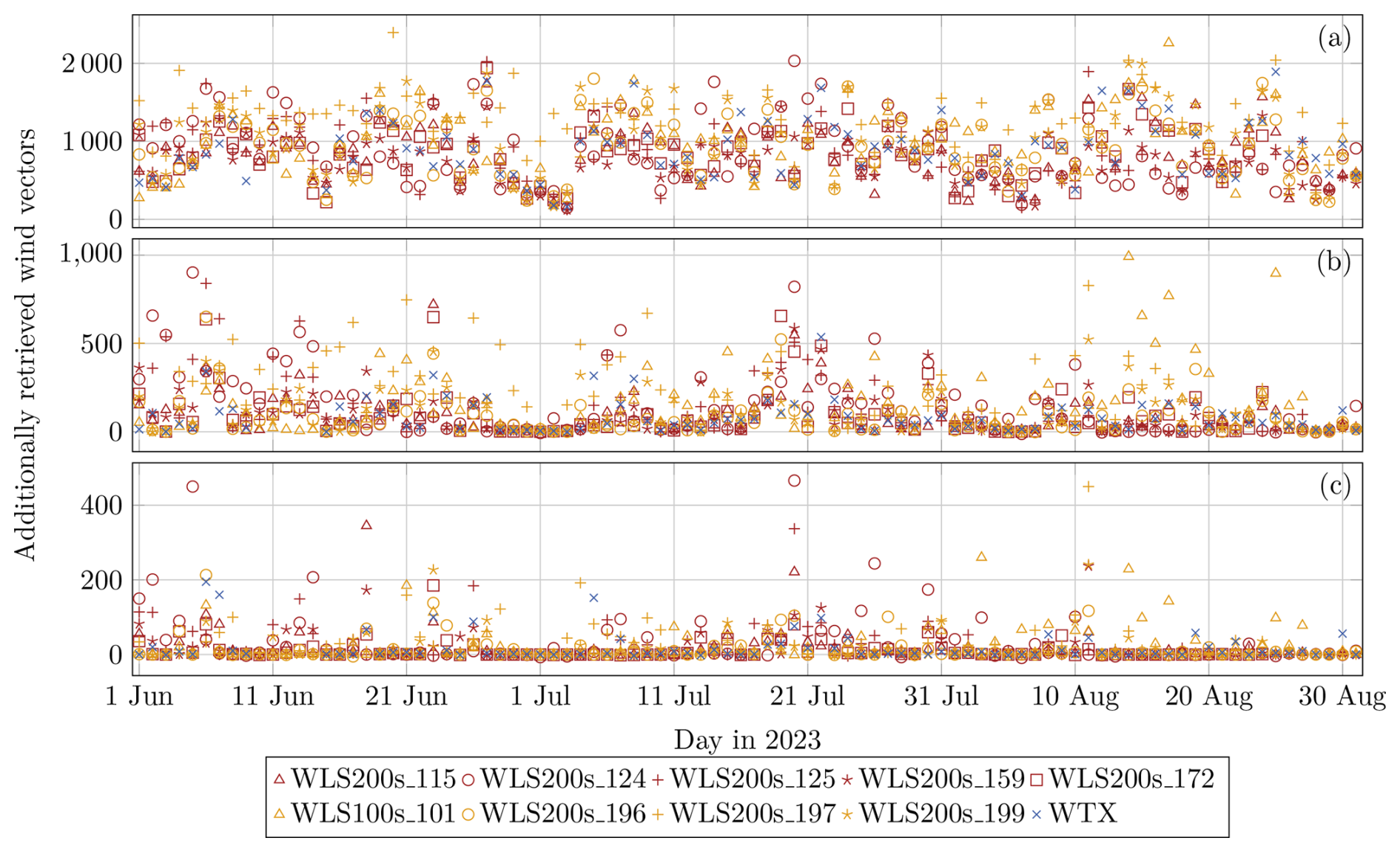
Figure 11 Number of additional wind vectors gained through the three iterations of modules 7.1 to 7.5. Results are provided on a daily basis for 10 Doppler lidars operated in the southern Black Forest (Germany) and neighbouring regions in Switzerland during a 3-month period in the summer of 2023. The difference is displayed between (a) the initial retrieval and iteration 1, (b) iteration 1 and iteration 2, and (c) iteration 2 and iteration 3.

5 Validation of the standard module chain

The wind profiles obtained using the standard module chain and settings, operated with 10 min temporal resolution and 100 m vertical resolution, are validated against radiosonde measurements for three different Doppler lidar systems at different locations. The Doppler lidar systems included for evaluation cover a Leosphere WLS200s, a Lockheed Martin WindTracer (WTX), and a Halo Photonics StreamLine XR+. The radiosondes used as a validation reference were released in the near surroundings of the respective Doppler lidar. The geographic and temporal distribution of the station data covers a wide range of atmospheric conditions, ensuring representativeness of the validation.

5.1 Data basis used for validation

The WLS200s wind profile retrieval results are compared with 180 ascending radiosondes between June and August 2023 at the MeteoSwiss site Payerne, Switzerland (46.81° N, 6.94° E). Heterogeneous scans of type DBS, step-and-stare, and sector PPIs are used for wind profile retrieval (Fig. E2a). The radiosondes were launched regularly at 11:00 and 23:00 UTC, thereby covering both daytime and nocturnal conditions.

The WTX wind profile retrievals are evaluated against 131 ascending radiosondes launched during the Swabian MOSES 2023 experiment at Villingen-Schwenningen, Germany (48.06° N, 8.49° E) (Kohler, 2025). The WTX conducted PPI scans (elevations of 3, 30, 60 °) alternating with RHI scans in directions from 0 elevation to 90 ° elevation in continuous-scan mode (Fig. E2b). Radiosondes were launched 3-hourly during eight intensive observation periods targeting the initiation of thunderstorms, thereby covering pre-convective and convective conditions with assumed strong spatial flow variability.

For the validation of the StreamLine XR+, publicly available lidar measurements (Schmithüsen et al., 2024) from the Neumayer Station, Antarctica (70.67° S, 8.27° W), are processed. The retrieved wind profiles are compared to 200 radiosondes usually released at 11:00 UTC between 4 January and 26 November 2024 (Schmithüsen, 2022). The lidar conducted a 12-beam step-and-stare pattern (Fig. E2c). Due to the remote Antarctic location, strong and vertically sheared katabatic flows and challenging lidar measurement conditions with low aerosol concentrations are covered.

An initial visual analysis of the wind profiles obtained using the WLS200s at Payerne and the WTX at Villingen-Schwenningen shows that physically plausible results are provided by the standard module chain. Hence, for these systems, there is no need for a reconfiguration of the standard module chain or the adaptation of thresholds. The results obtained for the Doppler lidar at Neumayer Station show a peculiar artefact: at weak SNR, very frequent vertical winds with −1 m s⁻¹ are observed in the absence of horizontal wind (i.e. horizontal wind speeds of approximately 0 m s⁻¹), visible in Fig. 8. Likely, a non-uniform radial velocity noise spectrum for measurements in weak-SNR conditions causes the observed effect. The observed phenomena and the applied solution are discussed in Appendix D. The ingestion of the suspicious radial velocities is prevented through an additional level 1 data filter applied for Neumayer Station, which excludes radial velocities between −2 and −0.35 m s⁻¹ for SNR values below −22 dB.

5.2 Retrieval validation for wind speed

A number of reasons complicate the validation of the lidar wind profile retrievals with radiosonde measurements, since a point-based in situ vertical profile is compared to a volume-based remote sensing retrieval. Non-homogeneous wind in time or space causes differences, as the retrieval represents an average over the aggregated time (10 min) and height, while the radiosonde ascents with approx. 5 m s⁻¹ and thereby crosses a 100 m height bin in approximately 20 s. To minimize the effect of spatial and temporal differences, the nearest temporal neighbour is used in the lidar vs. radiosonde comparison. Additionally, radiosondes may yield non-representative measurements and are advected with the flow. Hence, increasing spatial distances between the wind profiles may be present, especially at higher altitudes. Further, lidar-retrieved wind profiles suffer from retrieval errors due to flow inhomogeneity, depending on the scan patterns and atmospheric conditions (Gasch et al., 2020; Rahlves et al., 2022; Robey and Lundquist, 2022). Besides the differences in measurement characteristics, both systems may also suffer from direct measurement errors due to system imperfections.

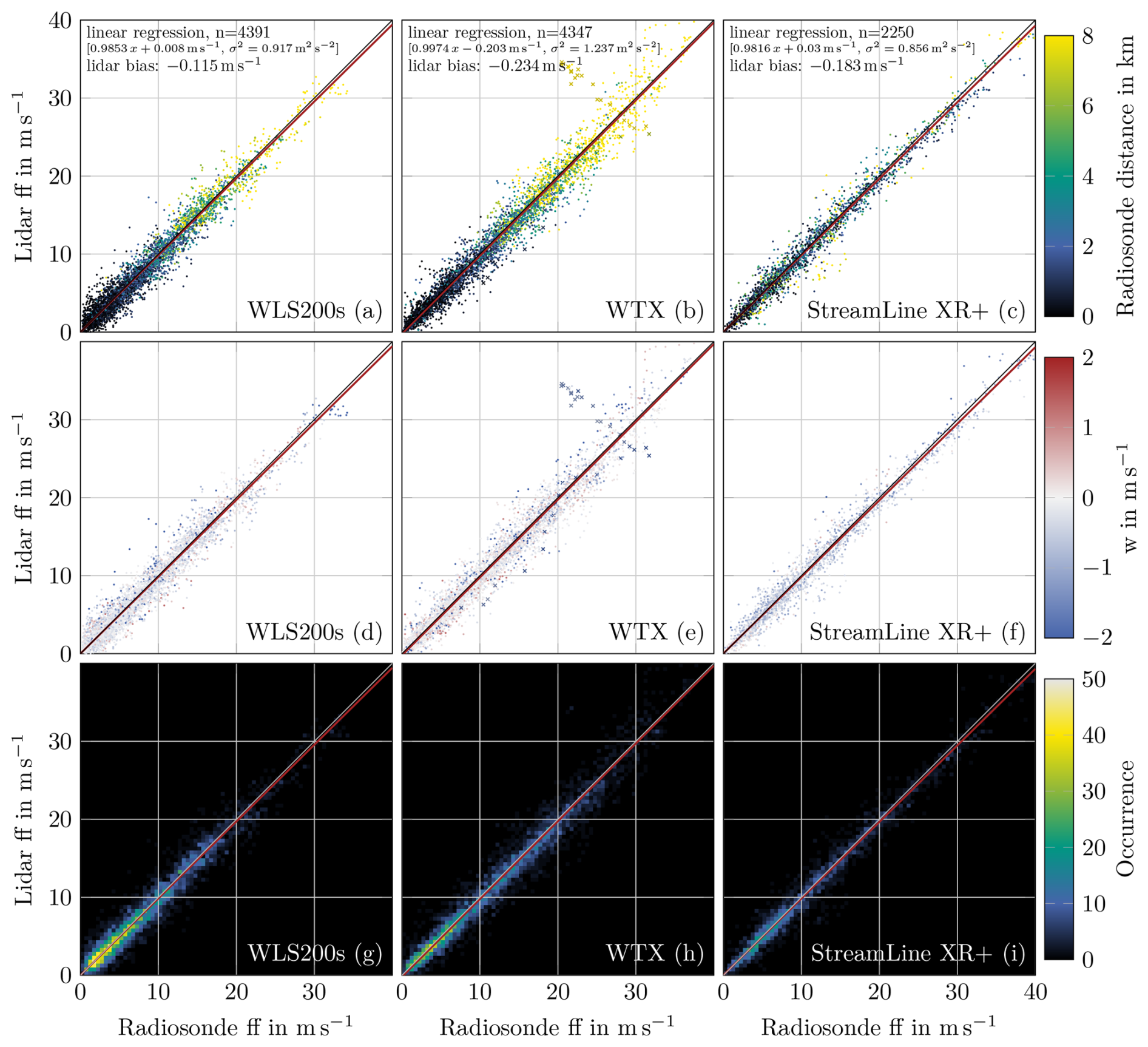
Figure 12 Agreement of the retrieved horizontal wind speeds with radiosonde measurements. An orthogonal distance regression is calculated for the Doppler lidars and radiosondes at Payerne (a, d, g), Villingen-Schwenningen (b, e, h), and Neumayer Station (c, f, i). The horizontal distance of the radiosonde to the lidar position (a–c), the retrieved vertical wind speed (d–f), and the occurrence in bins of 0.5 m s⁻¹ (g–i) are colour-coded. For Villingen-Schwenningen, one radiosonde profile is omitted from the comparison due to non-representative measurement conditions (displayed as crosses; see text).

Figure 12 shows the comparison of the radiosonde measurements with the corresponding retrieved horizontal wind speed for all three stations. WLS200s (Payerne) and WTX (Villingen-Schwenningen) exhibit good agreement over the full wind speed range. StreamLine XR+ (Neumayer) exhibits lower data availability but slightly higher agreement with the radiosondes. Deviations remain fairly constant in magnitude over the full wind speed range for all stations.

The WLS200s comparison at Payerne offers a representative data basis under various atmospheric conditions due to the regular operational launches without targeting of special atmospheric phenomena. Good agreement with a small positive bias of the wind speed retrieval is observed.

The deviations between radiosonde and lidar measurements are slightly larger at Villingen-Schwenningen, and more measurements under high-wind-speed conditions are included. The increased scatter is potentially related to the targeting of the radiosondes towards convective and pre-convective conditions, i.e. more spatial variability and less representative measurements. For the WTX, one radiosonde profile is omitted from the comparison (11 July 2023, 21:32 UTC) due to non-representative measurement conditions. An analysis of the corresponding meteorological situation reveals that the radiosonde was launched into a passing mesoscale precipitating system and, thus, encountered strongly non-representative conditions during its ascent and drift away from the lidar.

Similarly, the generally more stable atmospheric conditions at Neumayer introduce less spatial variability and hence provide more representative measurements, in addition to reduced lidar retrieval error due to more homogeneous flow.

For all stations, the largest deviations are frequently associated with non-zero vertical winds retrieved by the lidar (Fig. 12d–f). Comparisons with a negative vertical wind measured by the lidar in particular show an increased scatter. The increased scatter can be attributed to less homogeneous flow conditions, leading to less representative radiosonde measurements and increased lidar retrieval errors (Gasch et al., 2020; Rahlves et al., 2022; Robey and Lundquist, 2022). The retrieved negative vertical velocities are often associated with precipitation (snow, rain), which presents additional challenges for lidar measurements.

5.3 Retrieval validation for wind component profiles

For further validation including the vertical retrieval characteristics, the difference between the wind profiles retrieved from Doppler lidar measurements and radiosonde measurements is analysed. The retrieved wind profiles are compared to the radiosondes by subtracting the radiosonde's u and v component from the respective component of the retrieved Doppler lidar wind profiles. The resulting differences are shown for Payerne (WLS200s) in Fig. 13, for Villingen-Schwenningen (WTX) in Fig. 14, and for Neumayer Station (StreamLine XR+) in Fig. 15.

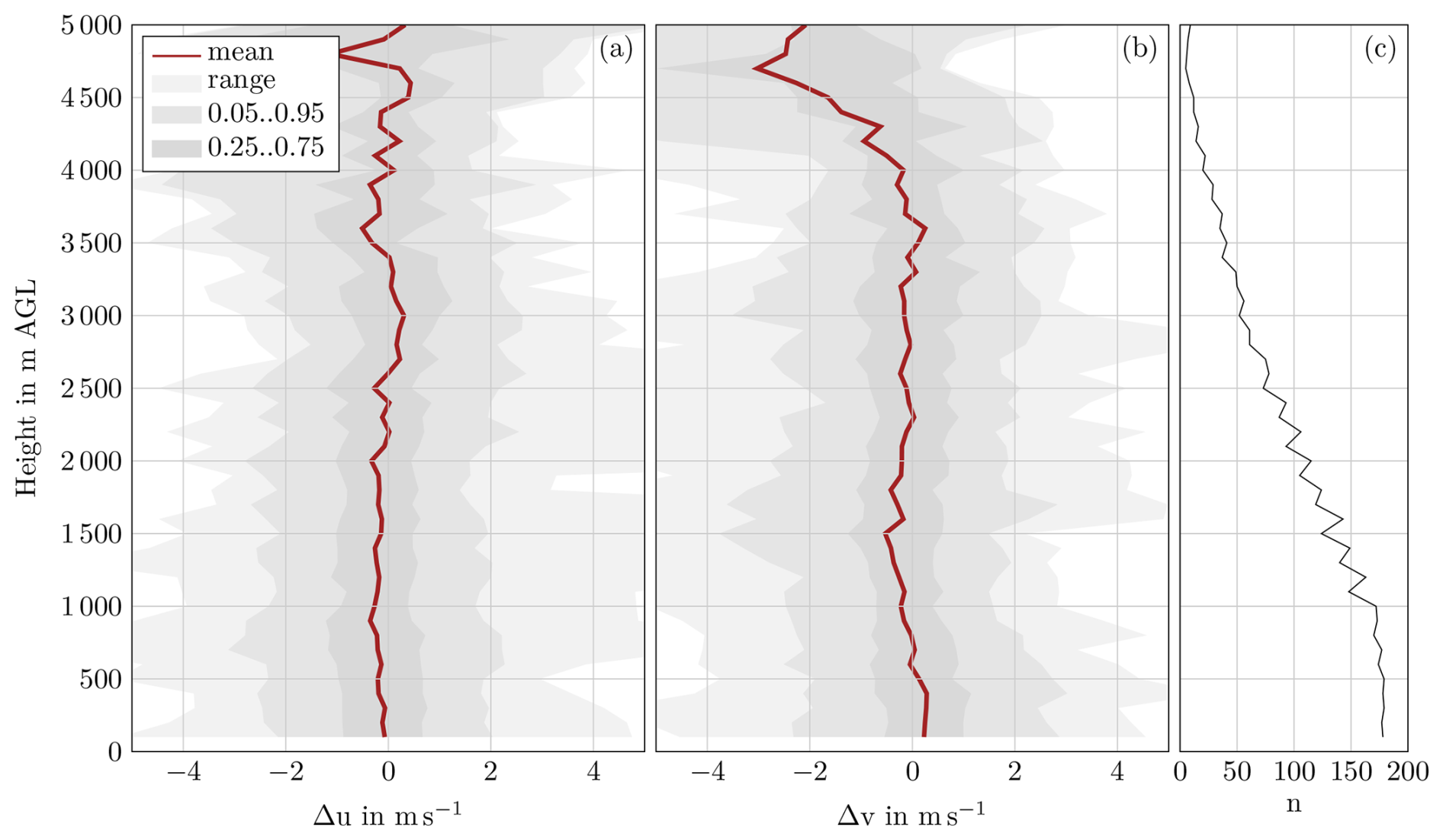
Figure 13 Horizontal wind component differences between radiosondes and WLS200s retrieval (10 min temporal resolution) at Payerne. The radiosonde wind components are subtracted from the retrieved Doppler lidar wind components. The shaded areas mark quantiles. The number of retrieved wind vectors n decreases with height.

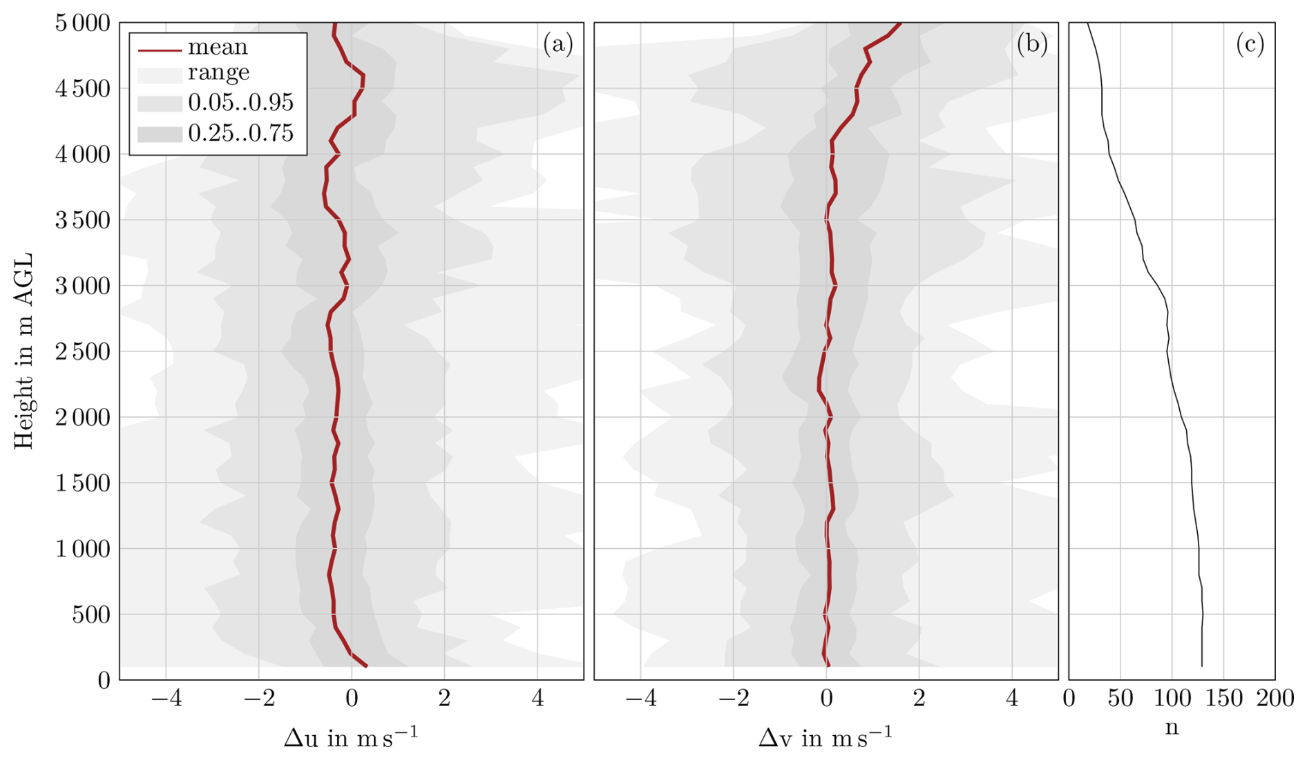
Figure 14 Horizontal wind component differences between radiosondes and wind profiles retrieved from the WTX Doppler lidar at Villingen-Schwenningen.

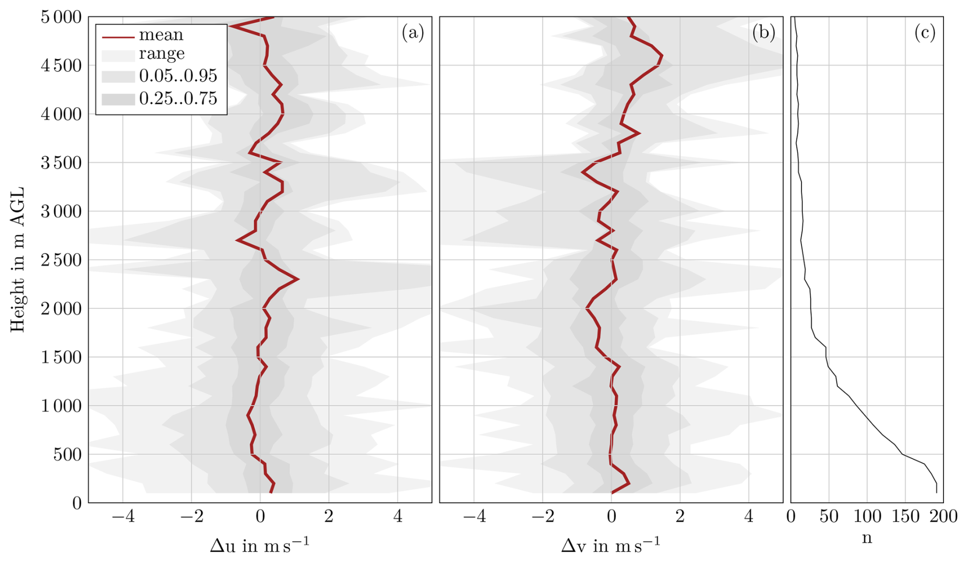
Figure 15 Horizontal wind component differences between radiosondes and the wind profiles retrieved from StreamLine XR+ located at the Neumayer Station at 10 min temporal resolution. The number of available samples n enables a reliable validation only at low heights.

For Payerne and Villingen-Schwenningen, the comparison shows good agreement between the wind profiles at altitudes with sufficient data availability below 4 km, especially when considering the varying footprints and distances between remote sensing and in situ measurements. The interquartile distance is stable with altitude, highlighting the consistent retrieval quality above the boundary layer, where only a reduced backscatter from aerosols is available. Larger differences are observed above 4 km, attributable to the insufficient sample size and large horizontal distances between the radiosondes and the Doppler lidar. The slight variation in the number of retrieved wind vectors with altitude for Payerne results from a different number of radial velocities mapped to the single height bins. Thereby, a higher wind vector availability for bins with more radial velocities is observed. Due to the targeted measurements at Villingen-Schwenningen, winds in the comparison are also predominantly from the west, resulting in elevated error levels in the u component compared to the v component.

The results of the StreamLine XR+ lidar at Neumayer Station, displayed in Fig. 15, also indicate good agreement at low heights, where the number of retrieved wind vectors is sufficient. The interquartile range is slightly reduced for the wind components at Neumayer Station, in agreement with the improved wind speed comparison compared to the other stations. However, more vertical variability is observed due to the smaller sample size, related to the often low aerosol concentrations in Antarctica.

5.3.1 The impact of temporal resolution

A small systematic difference (bias) in the u component of about −0.4 m s⁻¹ is evident for altitudes below 3 km at Villingen-Schwenningen, which is also detectable in the quartiles. No similar bias is observed in the v component and also not in any component at Payerne or Neumayer Station. Hence, the difference is likely attributable to local flow or representativeness effects. The u component shows systematically higher mean values, possibly creating sampling artefacts due to the occurrence of gusts. Wind gusts cause an increased wind speed for a limited time. The retrieved wind vectors consider, however, the complete interval of temporal aggregation, which is 10 min. The introduced consensus-based retrieval could smooth such gusts if the wind speed is significantly higher than during the majority of the temporal bin integration interval.

For comparison, the retrieval with a temporal resolution of 5 min is shown in Fig. E3. Using this higher resolution, the offset decreases slightly to about −0.3 m s⁻¹ and shows less variation up to 4 km height. Interestingly, the increase in temporal resolution does not increase retrieval errors noticeably. Instead, the interquartile range is similar or even slightly reduced. Since the WTX scan pattern was completed within 5 min, full scans are available even at this shorter averaging duration. Hence, the retrieval volume is explored equally well also for this temporal resolution. Nevertheless, even for full scans, one may expect less favourable averaging of the retrieval error due to turbulence in the retrieval volume (Robey and Lundquist, 2022; Rahlves et al., 2022). The fact that no increase in retrieval error is observed for shorter retrieval times illustrates the suitability of the scan pattern and the retrieval algorithm. Further, the expected slight increase in retrieval error due to turbulence may be compensated for by a smaller representativeness error in the comparison with the radiosonde. One reason may be the increased ability to capture short-term gusts for shorter retrieval periods (Steinheuer et al., 2022).

5.3.2 The impact of CNR on the retrieval quality

The standard module chain exploits additional radial velocity measurements with low CNR. In addition to visual plausibility checks, the distribution of the wind differences between radiosondes and the Doppler lidar depending on the CNR is evaluated. The differences in u and v depending on the CNR are displayed for all three locations in Fig. 16. Samples close to the weak CNR threshold are rare, since the CNR is the median of all measurements considered in the respective bin. Samples at the weak threshold would require the majority of the considered measurements to be at this threshold. Significant improvements in the availability of retrieved wind vectors due to the iterative procedure occur in the region between the conservative (ct) and the weak (wt) CNR threshold.

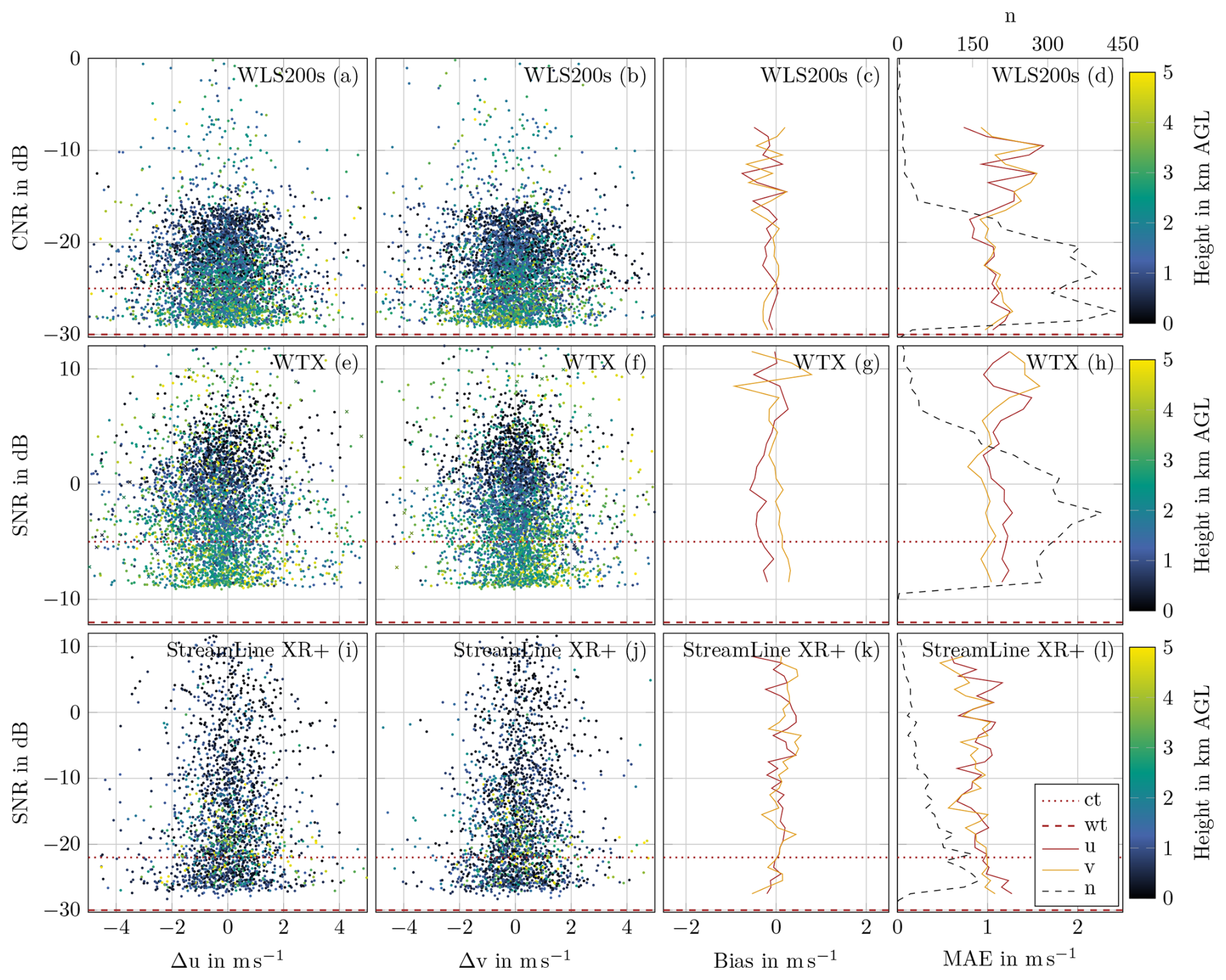
Figure 16 Horizontal wind component differences between radiosondes and wind profiles depending on the CNR. One sample represents a comparison for one radiosonde and one vertical bin. The mean bias and the mean average error (MAE) are calculated for u and v in bins of 1 dB width. The number of available samples n is displayed on the upper abscissa. Bias and MAE are omitted if n<10. The conservative (ct) and weak (wt) CNR thresholds are marked for the respective instruments. The lower ordinate limit corresponds to the weak CNR threshold in all subplots.

The height (colour-coded) needs to be considered alongside the CNR, since the two quantities are correlated. As expected, low CNR values occur predominantly for higher altitudes for the stations in Europe (Fig. 16a–h). The bias is close to ±0 m s⁻¹, except in u for the WTX (Fig. 16c, g, k). The bias of about −0.4 m s⁻¹ in the u component is already observed in Fig. 14 and discussed in the previous section. For CNR bins with a sufficient number of samples, the mean average error (MAE) is around ±1 m s⁻¹ for all CNR. For the WLS200s (a–d) and the StreamLine XR+ (i–l), a weak increase in the MAE can be observed for measurements with low CNR. The WTX (e–h) does not show this behaviour. A slight systemic increase in the deviation with decreasing CNR compared to the radiosonde measurements occurs for the concerned systems. However, the associated error cannot be clearly assigned to the Doppler lidar systems. Since low CNR values predominantly occur at higher altitudes, the increasing distance between the lidar and the radiosonde could also contribute to this effect. Figure E4 shows the same analyses for lidar to radiosonde distances instead of the CNR. Figure E5 shows the associated geographical position of the radiosondes during the comparisons. The weak increase in the MAE for increasing distances supports such a dependency on the distance to the radiosonde (Fig. E4d, h, l).

For the StreamLine XR+ in Antarctica, low CNR values are also predominant for low-altitude measurements (Fig. 16i–l). A high number of considered measurements below the −22 dB conservative CNR threshold is noteworthy. The share of additionally retrieved wind vectors at low CNR confirms the advantage of the standard module chain for regions with low backscatter.

6 Conclusions

A novel modular software tool for the retrieval of wind profiles from heterogeneous Doppler lidar measurements is introduced.

To enable the processing of measurements from various Doppler lidar systems, a standardized level 1 data format is used. The level 1 format provides data homogenization and enables subsequent retrieval of wind profiles using consistent processing routines, independent of the system origin. To maximize data availability, wind vectors are retrieved after binning the measured radial velocities with respect to time and height. Thus, all available measurements from various data acquisition settings and scan types can be exploited for the retrieval, independent of their origin.

The software architecture is designed in a modular way, enabling flexible adaptation without a need for coding. The data filtering and retrieval process is defined in module chains, in which the arrangement of modules specifies the processing steps and the variables' flow. Each module performs a dedicated calculation with defined input and output variables, as well as required parameters. A configuration file is used to provide or modify parameter values required by the modules during operation. The modular architecture enables high flexibility for adaptions with reduced development effort. The software framework is provided as open-source Python code.

Thus, the software is suitable for three types of users:

1. Users with a need for straightforward Doppler lidar wind profile retrievals can use the standard module chain configuration, which provides validated and quality-controlled wind profiles for common conditions and multiple Doppler lidar systems.

2. Users with special investigation purposes or uncommon measurement parameters can configure the module chain and parameters according to their interests and needs.

3. Developers can contribute their own algorithms in new modules.

The delivered standard module chain for common conditions comprises an initial retrieval of the wind profiles with reliable measurements, based on a conservative CNR filtering threshold. An iterative procedure adds measurements with a lower CNR, if the measurements are within the expected range of the extrapolated previously retrieved wind profiles and if a sufficient share of measurements supports the retrieved wind vector. Through the iterative procedure, quality-controlled wind profiles are provided for weak-CNR conditions as well.

Validation of the retrieved wind profiles is conducted for three different Doppler lidar systems at different locations. Atmospheric conditions ranging from summertime convective boundary layers to wintertime stable boundary layers in the Antarctic are investigated. The comparison with radiosonde measurements reveals a high quality of the retrieved wind profiles for all investigated Doppler lidars and atmospheric conditions.

Overall, the modular software package provides capabilities to implement different retrieval scenarios for a wide range of users, Doppler lidar systems, and applications. The introduced modular software architecture enables the flexibility to cover various application cases, on the one hand, but also ensures high-level traceability, which is essential for the processing history of measurements used in models, on the other hand.

Appendix A: Software configuration file example

A1 Module chain example

Module chains are configured in a JSON format. Adding or omitting modules is possible through removing or inserting the respective text blocks in the module chain file. An exemplary JSON-formatted representation for the module chain displayed in Fig. 5 is provided here.

[
    {
        "type":"calculation",
        "alias_name":"cnr_filter",
        "module_name":"Flag_variable_limits_l1",
        "rename_parameters": {
            "min_value":"cnr_threshold_dB"
        },
        "rename_level1_inputs": {
            "variable":"CNR"
        },
        "rename_level1_outputs": {
            "condition_met":"validity_
                probability"
        }
    },
    {
        "alias_name":"retrieve_wind_vectors",
        "type":"calculation",
        "module_name":"Bin_retrieve_uvw"
    },
    {
        "alias_name":"final_nc_export",
        "type":"export",
        "module_name":"NetCDF_l2"
    }
]

The module chain consists of three JSON objects, each representing one module (see Fig. 5).

Table A1 The presented parameters are needed for the standard module chain and can be modified in the settings file.

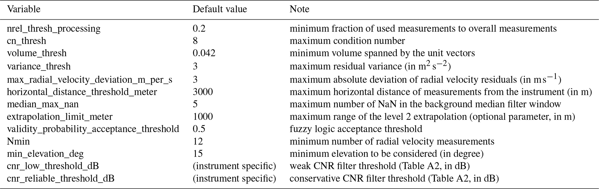
The first module (alias name cnr_filter) implements a CNR filter by setting the flag variable validity_probability to 1.0 if the CNR value is at least the threshold specified in the parameter cnr_threshold_dB. Otherwise, the value of validity_probability is 0.0. The calculation module used for the implementation of the CNR filter is Flag_variable_limits_l1. This module uses min_value as default parameter for the minimum threshold, a variable with the name variable as default level 1 input, and a variable with the name condition_met as default level 1 output. Therefore, the default names for the parameter, the level 1 input, and the level 1 output are renamed for the use as CNR filter. This renaming is possible by specifying rename_parameters, rename_level1_inputs, and rename_level1_outputs for this module.

The second module (Bin_retrieve_uvw) calculates the level 2 wind vectors using the level 1 radial velocities where the value of validity_probability is 1.0. No renaming of variables or parameters is needed, as the default names are used.

The third module (NetCDF_l2) exports the final level 2 dataset to a netCDF file.
Parameters are specified in the settings file (Appendix A2). The user is requested to insert unspecified parameters in an interactive dialogue before the module chain is executed.

A2 Settings file and configuration parameters

The settings file contains processing settings, including directories and parameters. An *.ini file containing the settings is specified for the software execution. Import and export settings are specified in separate import and export sections of the *.ini file. Parameters can be applied to all modules with the prefix global. or to a single module by using the module's alias name, followed by a dot as prefix. Parameters are specified in the section parameters of the *.ini file. Instrument-type-specific or instrument-specific sections allow the user to adapt settings for individual instrument types or instruments. Details are provided in the manual. To specify the level 2 dataset, the following parameters are mandatory for all module chains:

• AtmoProKIT_parameter_temporal_aggregation_seconds
  (default value: 600)

• AtmoProKIT_parameter_vertical_aggregation_meter
  (default value: 100)

• AtmoProKIT_parameter_offset_first_bin_meter
  (default value: −50)

• AtmoProKIT_parameter_max_height_meter
  (default value: 5050).

Further parameters can be required by the modules contained in the module chain. The parameters required by the single modules are listed in the manual. The parameters needed for the standard module chain are listed in Table A1.

A2.1 Settings file example for the simple retrieval

[import]
level1_netcdf.level1_import_directory=/home/
    user/Level1
level1_netcdf.level1_variables=["radial_
    velocity","CNR","elevation","azimuth",
    "range"]

[export]
global.level2_export_directory=/home/user/
    Level2

[parameters]
global.AtmoProKIT_parameter_temporal
    _aggregation_seconds=600
global.AtmoProKIT_parameter_vertical
    _aggregation_meter=100
global.AtmoProKIT_parameter_offset
    _first_bin_meter=-50
global.AtmoProKIT_parameter_max
    _height_meter=5050
global.nrel_thresh_processing=0.2
global.cn_thresh=8
global.volume_thresh=0.042
global.variance_thresh=3
global.max_radial_velocity
    _deviation_m_per_s=3
global.Nmin=12
global.validity_probability
    _acceptance_threshold=0.5

[parameters_instrument_type.WLS200s]
global.cnr_threshold_dB=-25

A2.2 Parameters used in the standard module chain

The parameters needed for the standard module chain are listed in Table A1.

Table A2 Default values for the conservative CNR threshold (cnr_reliable_threshold_dB) and the weak CNR threshold (cnr_low_threshold_dB) used in the settings file.

Appendix B: Variable flow in the standard module chain

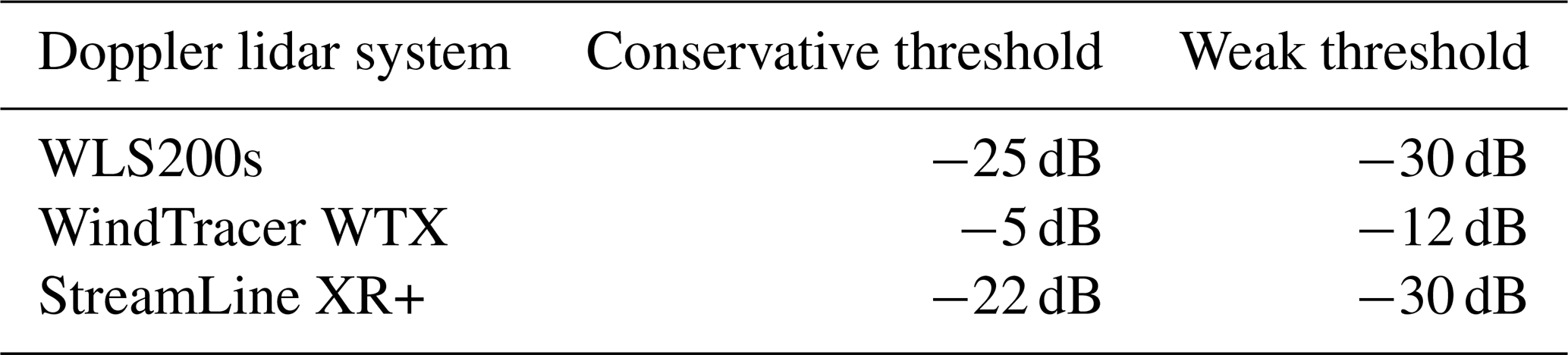
Table B1 Variable flow in the standard module chain. Coordinates and related variables are omitted in this listing. Read access (r) and write access (w) are indicated for the module numbers introduced in Table 1. Compared to module 6, module 7.5 provides additional statistical evaluations of the CNR and the Doppler spectrum width and adds the respective quality indicators to the level 2 dataset.

Appendix C: Wind profile retrieval theory

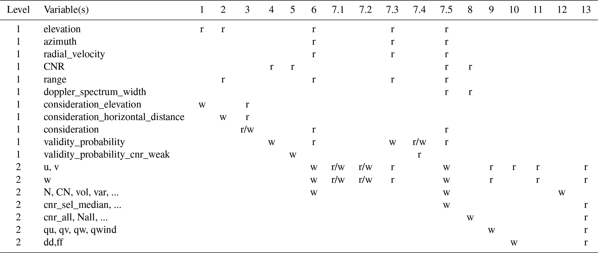
Calculating the least-squares fit to retrieve wind vectors from measured radial velocities is an established approach (e.g. Päschke et al., 2015; Teschke and Lehmann, 2017; Zentek et al., 2018; Bell et al., 2020; Steinheuer et al., 2022; Gebauer and Bell, 2024). For the calculation of one wind vector ${\mathit{v}}_{\mathrm{p}}=(u,v,w{)}^{\mathrm{T}}$, a projection onto the multiple radial velocity measurements ${\mathit{V}}_{\mathrm{r}}=(V_{\mathrm{r}\mathrm{1}},\mathrm{\dots },V_{\mathrm{r}n}{)}^{\mathrm{T}}$ is required, which is displayed in Eq. (C1). The system of equations (Eq. C1) projects the wind vector components u, v, and w onto the radial velocities $V_{\mathrm{r}\mathrm{1}},\mathrm{\dots },V_{\mathrm{r}n}$ depending on the given angular position of the scanner (azimuth α, elevation angle above the horizontal plane ϵ).

$$\begin{array}{}\text{(C1)}& \begin{array}{rl}& \left(\begin{array}{ccc}\sin \left({\mathit{\alpha }}_{\mathrm{1}}\right)\cos \left({\mathit{ϵ}}_{\mathrm{1}}\right)& \cos \left({\mathit{\alpha }}_{\mathrm{1}}\right)\cos \left({\mathit{ϵ}}_{\mathrm{1}}\right)& \sin \left({\mathit{ϵ}}_{\mathrm{1}}\right)\\ \mathrm{⋮}& \mathrm{⋮}& \mathrm{⋮}\\ \sin \left({\mathit{\alpha }}_n\right)\cos \left({\mathit{ϵ}}_n\right)& \cos \left({\mathit{\alpha }}_n\right)\cos \left({\mathit{ϵ}}_n\right)& \sin \left({\mathit{ϵ}}_n\right)\end{array}\right)\\ & \cdot \left(\begin{array}{c}u\\ v\\ w\end{array}\right)=\left(\begin{array}{c}{V}_{\mathrm{r}\mathrm{1}}\\ \mathrm{⋮}\\ V_{\mathrm{r}n}\end{array}\right).\end{array}\end{array}$$

This relation can be expressed in the following way:

$$\begin{array}{}\text{(C2)}& \mathbb{G}\cdot {\mathit{v}}_{\mathrm{p}}={\mathit{V}}_{\mathrm{r}}.\end{array}$$

This equation system is overdetermined for more than three measurements. Thereby, a retrieval of the wind vector is possible through minimizing the least-squares sum of the residuals.

The residuals δ describe the deviation of the measured radial velocities from the wind vector v_p. The residuals are

$$\begin{array}{}\text{(C3)}& \mathit{\delta }=\mathbb{G}\cdot {\mathit{v}}_{\mathrm{p}}-{\mathit{V}}_{\mathrm{r}}.\end{array}$$

To receive the least-squares fit of v_p, the sum of the squared residuals s has to be minimized. It is

$$\begin{array}{}\text{(C4)}& s={\mathit{\delta }}^{\mathrm{T}}\cdot \mathit{\delta }.\end{array}$$

This least-squares fit problem can be solved by multiplying the Moore–Penrose pseudoinverse (Päschke et al., 2015; Menke, 2012)

$$\begin{array}{}\text{(C5)}& {\mathbb{G}}^{+}=({\mathbb{G}}^{\mathrm{T}}\mathbb{G}{)}^{-\mathrm{1}}{\mathbb{G}}^{\mathrm{T}}\end{array}$$

from the left to Eq. (C2), which finally results in

$$\begin{array}{}\text{(C6)}& {\mathit{v}}_{\mathrm{p}}={\mathbb{G}}^{+}\cdot {\mathit{V}}_{\mathrm{r}}.\end{array}$$

An alternative calculation of the pseudoinverse using the matrices obtained with the singular value decomposition of 𝔾 is less susceptible to errors for poorly conditioned 𝔾 (Boccippio, 1995). Therefore, algorithms usually calculate the pseudoinverse (Menke, 2012)

$$\begin{array}{}\text{(C7)}& {\mathbb{G}}^{+}={\mathbb{W}}_{\mathrm{p}}{\mathbb{S}}_{\mathrm{p}}^{-\mathrm{1}}{\mathbb{U}}_{\mathrm{p}}^{\mathrm{T}},\end{array}$$

where 𝕎_p, 𝕊_p, and 𝕌_p are submatrices of 𝕎, 𝕊, and 𝕌, and

$$\begin{array}{}\text{(C8)}& \mathbb{G}=\mathbb{U}\mathbb{S}{\mathbb{W}}^{\mathrm{T}}\end{array}$$

is the singular value decomposition of 𝔾. 𝕊_p is a diagonal matrix of the singular values of 𝔾, which is $\mathrm{diag}({\mathit{\lambda }}_{\mathrm{1}},{\mathit{\lambda }}_{\mathrm{2}},{\mathit{\lambda }}_{\mathrm{3}})$ for the present problem.

𝕊_p is also needed for the calculation of the CN. Usually, 𝕊_p is calculated with λ₁, λ₂, and λ₃ in descending order (Menke, 2012), which is also the case in the NumPy implementation (https://numpy.org/doc/stable/reference/generated/numpy.linalg.svd.html, last access: 5 November 2024) used in the present software. The condition number CN is the maximum singular value divided by the minimum singular value (Boccippio, 1995), which is

$$\begin{array}{}\text{(C9)}& \mathrm{CN}={\displaystyle \frac{{\mathit{\lambda }}_{\mathrm{1}}}{{\mathit{\lambda }}_{\mathrm{3}}}}.\end{array}$$

Appendix D: Extension of the standard module chain for Neumayer Station

The StreamLine XR+ at Neumayer Station exhibits peculiar, temporally, and vertically extensive regions with vertical winds of approx. −1 m s⁻¹, without apparent background wind (i.e. horizontal wind speeds of approx. 0 m s⁻¹). Figure D1 shows an example of this effect. The corresponding SNR is displayed in Fig. D2. While some of the retrievals could be physical, e.g. due to snowfall in quiescent air, the continuity and frequent occurrence of the vertical winds without horizontal winds is implausible. Closer analysis reveals that the vertical velocities are attributable to frequent radial velocity measurements around −1 m s⁻¹ during weak-SNR conditions below −22 dB (Fig. 8c). Since the −1 m s⁻¹ radial velocity measurements are independent of the scanning direction (i.e. also azimuth direction), no horizontal winds and solely vertical winds are retrieved if the −1 m s⁻¹ measurements present the overwhelming majority of measurements.

The non-uniform distribution of radial velocity measurements during weak-signal conditions is traceable to a previously unreported issue of the StreamLine XR+ at Neumayer Station. Internal system issues (e.g. electro-magnetic interference of hardware components) likely contaminate the spectrum used for radial velocity estimation (Holger Schmithüsen, Markus Kayser, Johannes Bühl, Ronny Engelmann, Martin Radenz, personal communication, 2024). Since the raw spectrum data are not available, the radial velocity estimation cannot be improved through an improved background noise correction and subsequent reprocessing in this study.

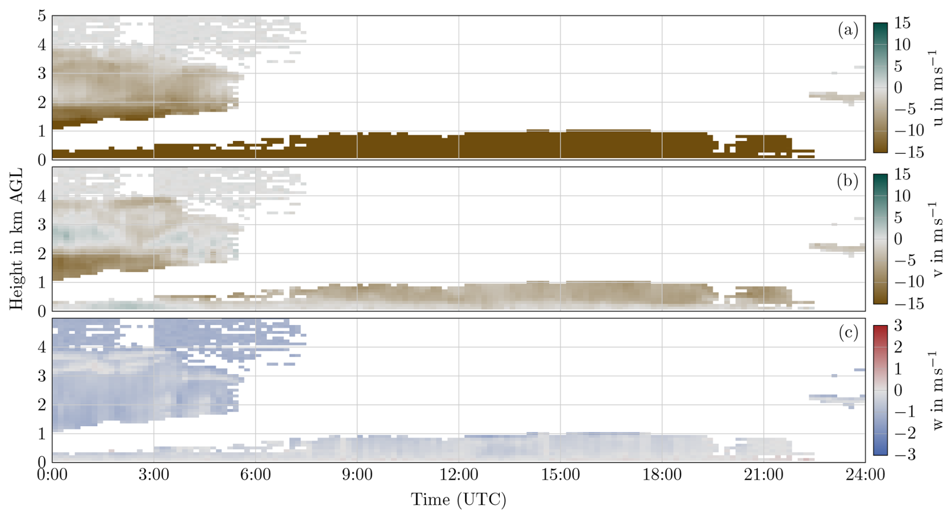
Figure D1 Result of the standard module chain applied for the StreamLine XR+ at Neumayer Station on 19 May 2024. A number of wind vectors indicate a vertical wind of −1 m s⁻¹ without horizontal wind. The reason is a peak in the radial velocity noise distribution around −1 m s⁻¹.

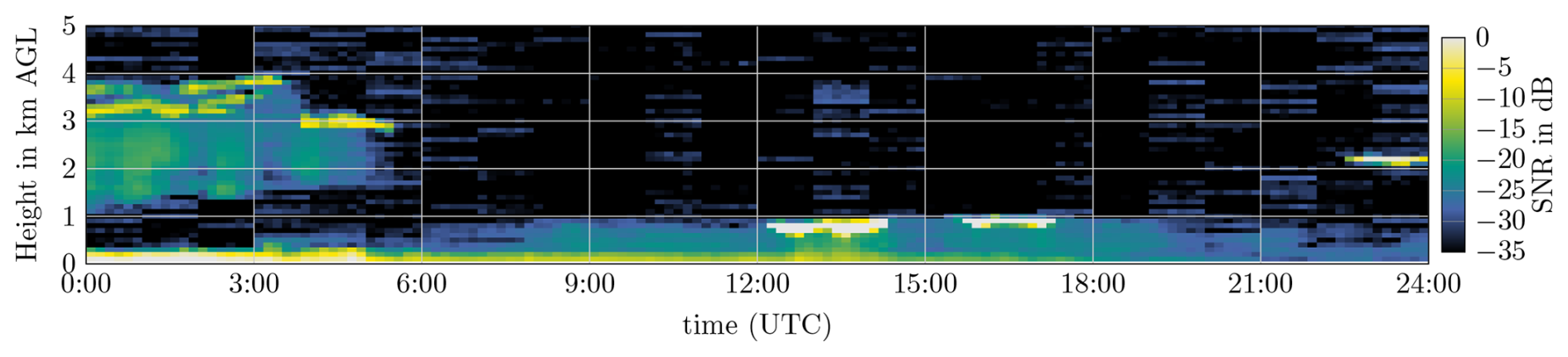
Figure D2 Doppler lidar SNR at Neumayer Station on 19 May 2024. The median of the SNR values of all measurements available per bin is displayed.

Nevertheless, StreamLine XR+ wind profiles from Neumayer Station are included in the radiosonde comparison since they serve to show both a limitation and an advantage of the presented modular wind profile retrieval software. First, the software should not be used to process Doppler lidar data irrespective of data quality, without the operator's reflection on the provided results. The consensus approach used in the least-squares fit retrieval and the background wind estimation rely on a broad distribution of radial velocity noise. In the Neumayer case, only user experience and meteorological reasoning allow judging the frequent −1 m s⁻¹ radial velocity measurements as implausible, a task which cannot be provided by the software. Second, if an issue with the data is identified, the modular software can be easily adapted to deal with the problem. In the Neumayer case, an additional level 1 consideration flag is introduced in the module chain: radial velocities between −2 and −0.35 m s⁻¹ are excluded if they exhibit an SNR below −22 dB. This filter prevents ingestion of the contaminated radial velocities prior to wind vector retrieval but still allows for retrieval even in weak-SNR conditions with the remaining measurements.

Figure D3 Result of the extended standard module chain applied for the StreamLine XR+ at Neumayer Station on 19 May 2024. Radial velocities between −2 and −0.35 m s⁻¹ are excluded from the retrieval for SNR below −22 dB. Implausible wind vectors which appear in Fig. D1 are rejected.

Appendix E: Additional figures

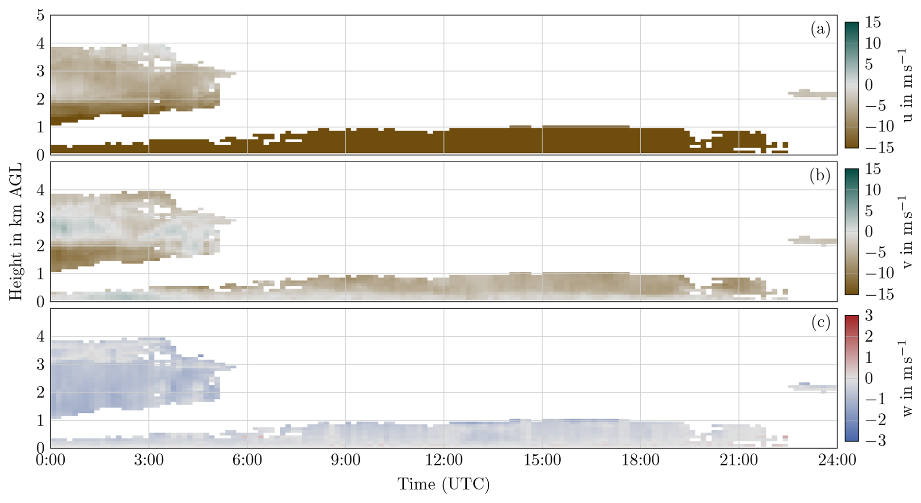
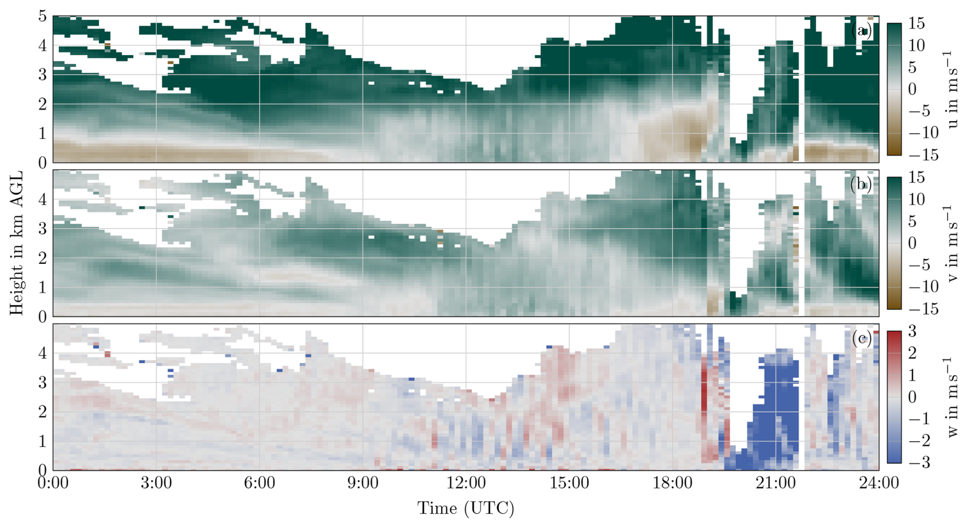
Figure E1 Simple retrieval considering measurements with a CNR threshold of −30 dB. As no confidence background is applied, transient conditions (at 20:00 UTC in particular) are covered better than in Fig. 10. However, some erroneous wind vector retrievals are also incorporated.

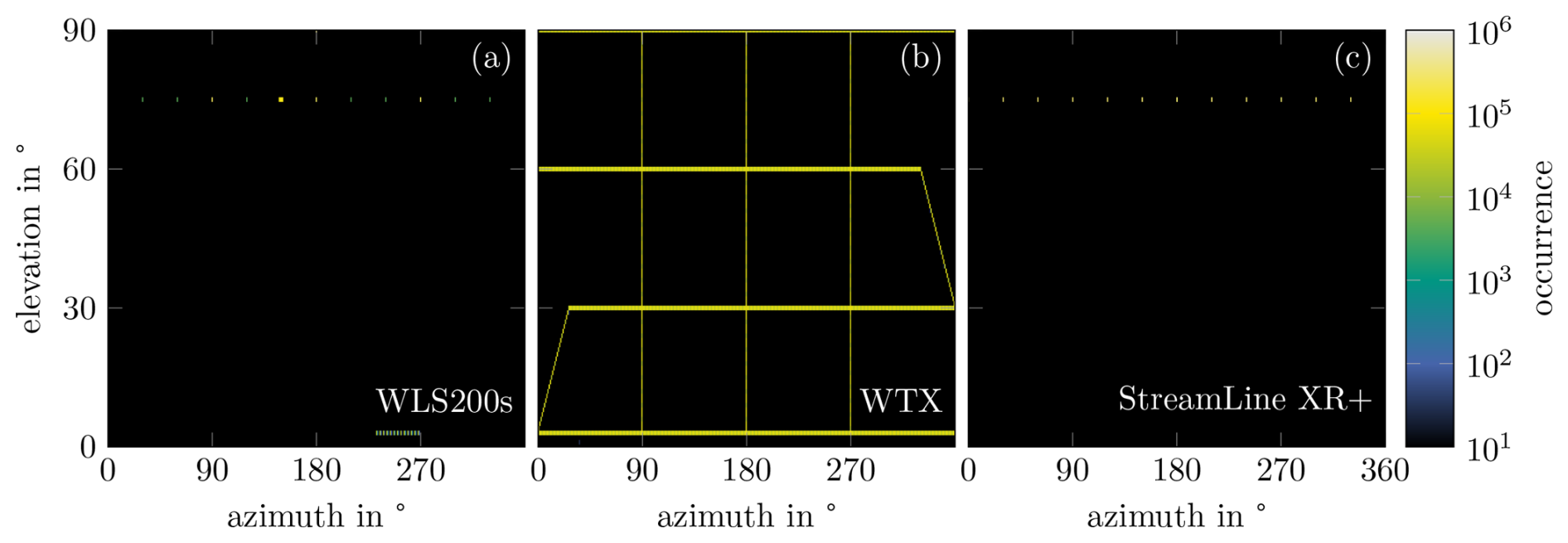
Figure E2 Occurrence of azimuth and elevation scan angles for WLS200s at Payerne (a), WTX at Villingen-Schwenningen (b), and StreamLine XR+ at Neumayer Station (c). All angles are summed up in bins of 1° between June and August 2023 for (a) and (b) and between 3 January and 26 November 2024 for (c).

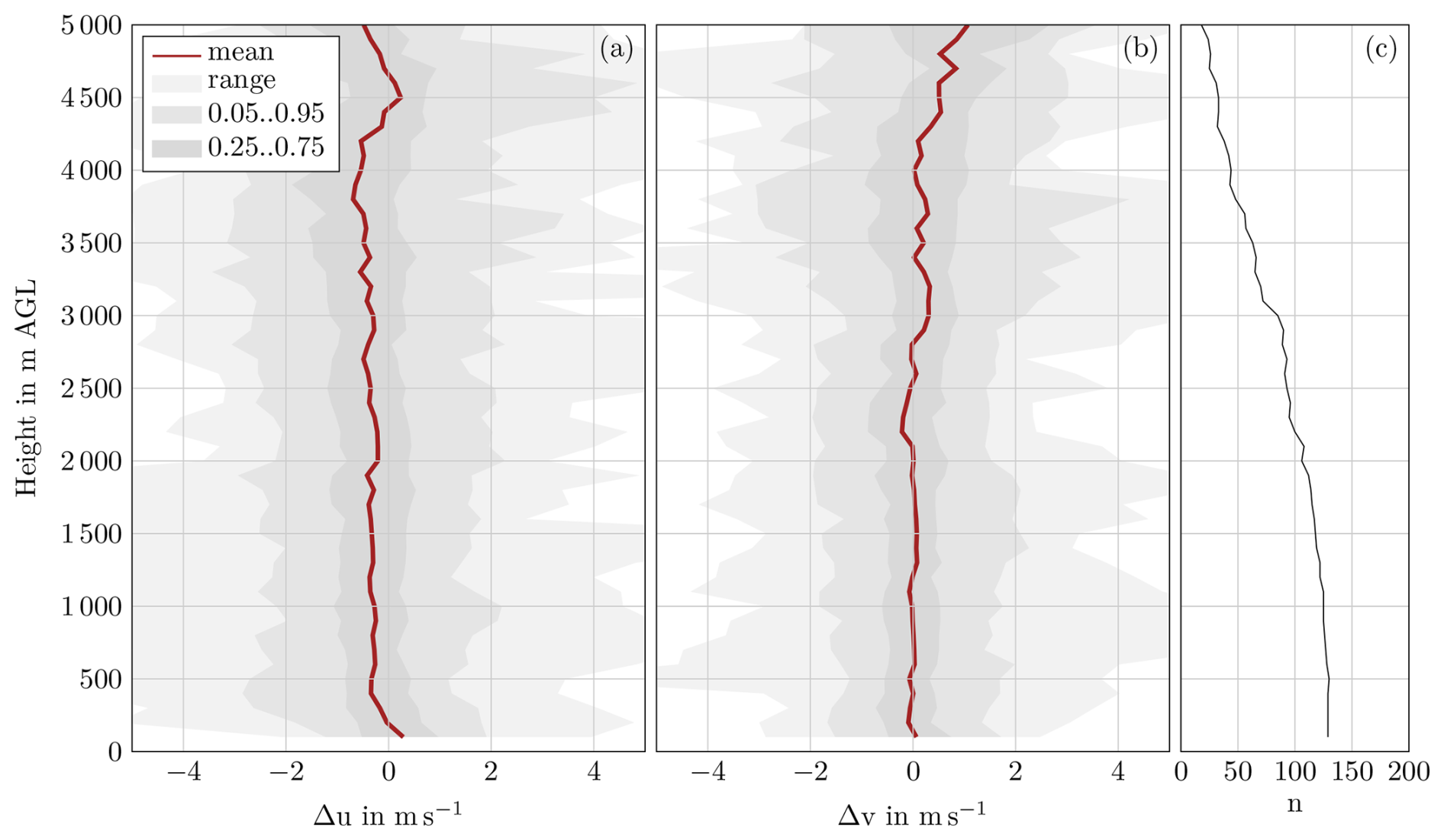
Figure E3 Horizontal wind component difference between radiosondes and the WTX retrieval at Villingen-Schwenningen. The same situation as in Fig. 14 is shown, however, at an increased temporal resolution of 5 min of the lidar retrieval.

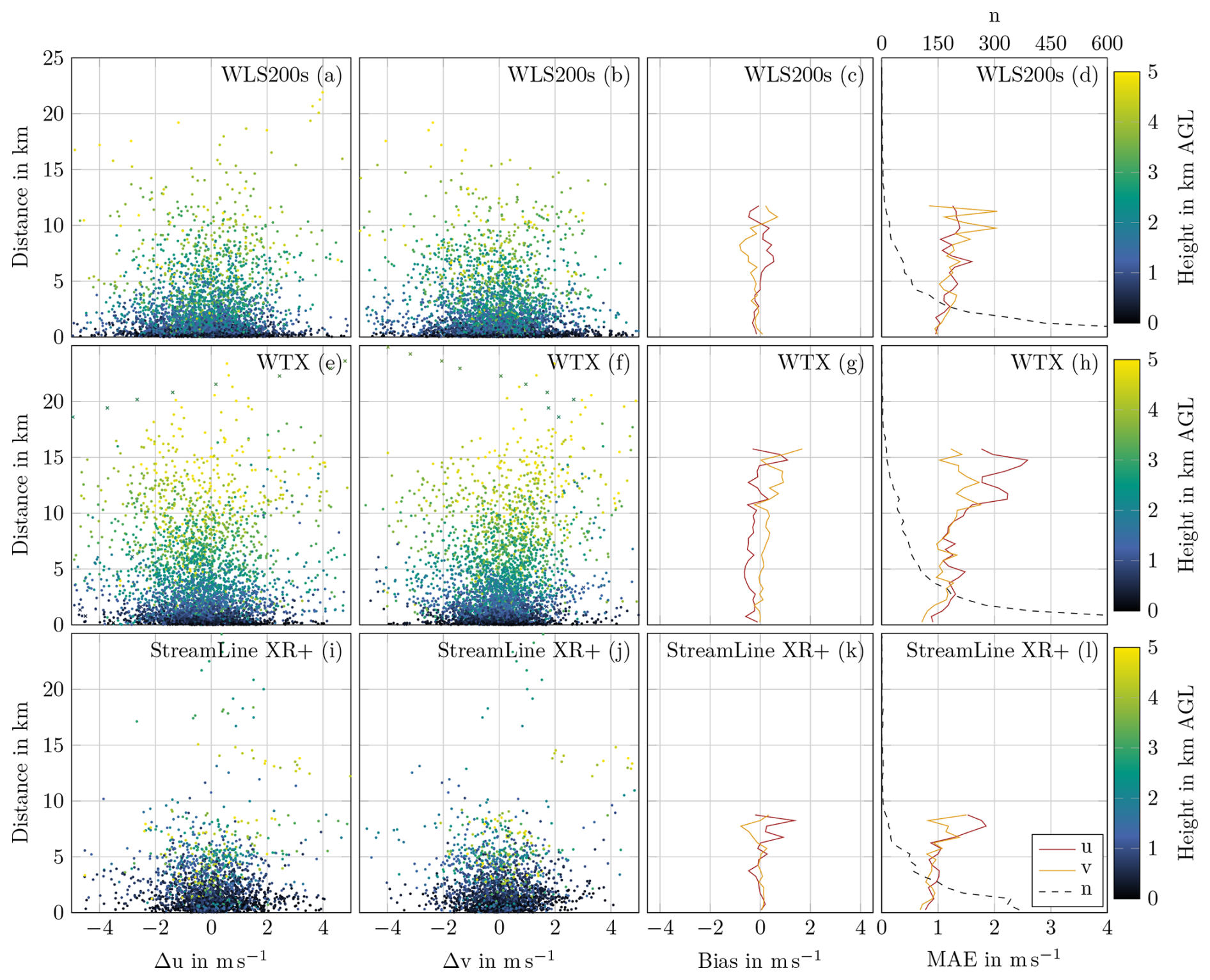
Figure E4 Horizontal wind component differences between radiosondes and retrieved wind profiles as a function of the horizontal distance between Doppler lidar and radiosonde. Bias and MAE are calculated for a number of samples n≥10. The MAE indicates a slight increase with increasing distance until about 10 km. For longer distances, the decreasing number of samples n causes high fluctuations.

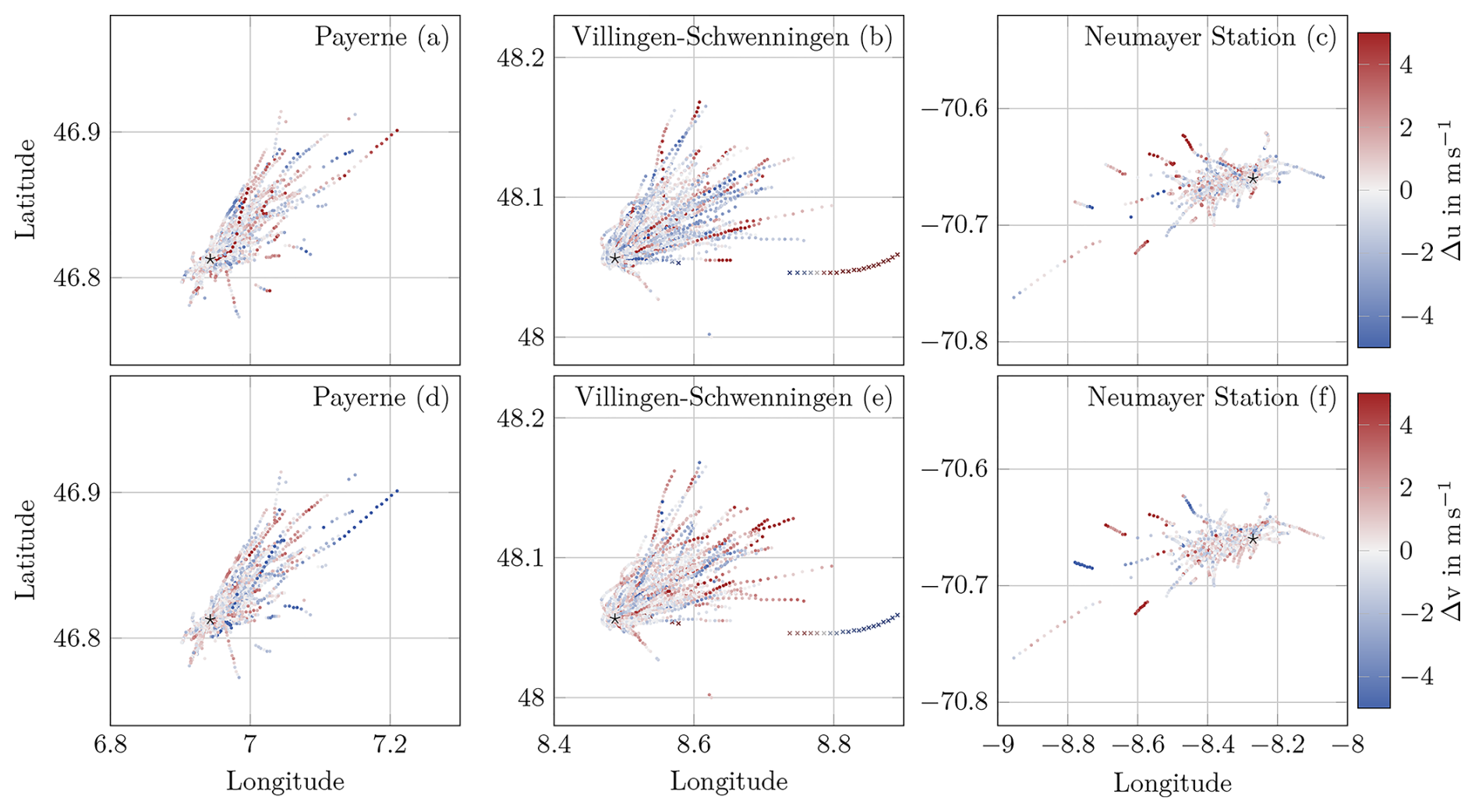
Figure E5 Positions of the radiosondes during the comparison with the Doppler lidars. Differences in the horizontal wind component u (a–c) and v (d–f) are colour-coded. The positions of the Doppler lidars WLS200s at Payerne (a, d), WTX at Villingen-Schwenningen (b, e), and StreamLine XR+ at Neumayer Station (c, f) are marked with a star.