A Bayesian statistical method to estimate the climatology of extreme temperature under multiple scenarios: the ANKIALE package

We describe an improved method and the associated package for estimating the statistics of temperature extremes in a Bayesian framework. Building on previous work, this method uses a range of climate model simulations to provide a prior of the real-world changes, and then considers observations to derive a posterior estimate of past and future changes. The new version described in this study makes it possible to process several scenarios simultaneously, while keeping one single counterfactual world (i.e., the world without human influence). We offer a free licensed, easy-to-use command-line tool called ANKIALE (ANalysis of Klimate with bayesian Inference: AppLication to extreme Events), which can be used to reproduce the analyses presented here, as well as to process user-defined events. ANKIALE is based on a python code, but is designed to be used from the command line interface. ANKIALE is natively parallel, enabling it to be used on a personal computer as well as on a supercomputer. To derive the posterior, ANKIALE uses state of art MCMC-methods to sample the posterior distribution. The potential of this method and tool is illustrated via an application to maximum temperature over Europe between 1850 and 2100 (the posterior is derived from ERA5, covering the period from 1940 to 2024), at a 0.25° resolution, for a range of four emission scenarios, including a particular focus on the city of Paris (France).

1 Introduction

Heatwaves are extreme phenomena whose frequency and intensity have increased with global warming (see, e.g. Seneviratne et al., 2021; IPCC, 2022a). Humans (see, e.g. Campbell et al., 2018; Huang et al., 2022; Masselot et al., 2023), plants (see, e.g. Hatfield and Prueger, 2015; Brás et al., 2021), ecosystems (see, e.g. Bastos et al., 2021) and infrastructure (see, e.g. Zuo et al., 2015), can suffer significant damage beyond certain thresholds, so it has become necessary to be able to predict and anticipate these events. Over recent decades, these findings have led to the development of the so-called extreme event attribution studies, which consist in establishing the weight of human influence in the occurrence or intensity of an extreme event (Perkins-Kirkpatrick et al., 2024). A number of methods and protocols have been developed (see, e.g. Ribes et al., 2020; Philip et al., 2020; Robin and Ribes, 2020a) which have enabled the analysis and attribution of a number of extreme events. The World Weather Attribution (WWA, 2024) group has specialized in producing attribution studies within a short time (typically within a week) following the occurrence of an event. Notable examples include the heatwave in Siberia in 2020 (Ciavarella et al., 2021), the heatwave in the USA and Canada in 2021 (Philip et al., 2022), and the wet heatwave in India in 2023 (Zachariah et al., 2023b). Other types of event can also be analyzed, such as extreme rainfall (Zachariah et al., 2023a, 2024; Clarke et al., 2024b), drought (Clarke et al., 2024a), or wildfire (Barnes et al., 2023), and others.

The attribution methods listed above typically infer the climatology (i.e. the statistical distribution) of the extremes of interest by assuming that the maxima of a variable (such as annual temperature) follow a Generalized Extreme Value distribution (see, e.g. Coles, 2001). This distribution is characterized by three parameters, which vary with external forcings (such as global or regional mean temperature). This statistical model is inferred either independently from observations, from climate models (Philip et al., 2020), or from both.

Several recent studies have proposed to implement the latter option, i.e., combining models and observations, within a Bayesian framework. In this context, a synthesis of climate models is used as a prior of the reality, and then observations are used to derive the posterior distribution of past and future changes. For example, Harris et al. (2013) proposes a Bayesian approach to predicting regional climate change. Several methods for synthesizing climate models have also been proposed by Sanderson et al. (2015), Knutti et al. (2017), and Brunner et al. (2019). Brunner et al. (2020) also provides a summary of different observational constraint methods. More recently, Smith et al. (2021) studied an observational constraint approach on an Energy Balance Model trained on multiple CMIP6 models to derive estimates of historical aerosol forcing. Zeder et al. (2023) studied the effect of short observations on the statistics of extreme events considering a Bayesian approach. Finally, Auld et al. (2023) also works on the changes in the distribution of the annual maximum daily maximum temperature (TXx) over Europe with CO₂ as covariate.

We describe several improvements to the Robin and Ribes (2020a) and Ribes et al. (2022) method, where the Bayesian approach enables the estimation of the statistics of extremes at the end of the century according to a climate scenario and conditioned on observed data over the historical period. Firstly, the statistical method has to be re-run separately for each emission scenario considered, with no guarantee for consistency across scenarios, especially for the confidence intervals. In particular, the inferred counter-factual world (i.e., the world without human influence), is different according to the scenario, leading to communication issues for key attribution diagnoses such as the probability ratio. Our improved implementation enables us to infer all scenarios simultaneously, which ensures that only one counterfactual world is calculated. Second, we revise the sampling procedure – based on a Metropolis Hasting Monte-Carlo (MCMC Metropolis et al., 1953; Hastings, 1970) method –, to make it consistent with recent progress in the Bayesian community. This revised implementation runs much faster than the previous one, and offers many guarantees in terms of properties and convergence of the MCMC chain.

The improved method comes with a deeply revised python package and command-line tool. The original method of Robin and Ribes (2020a) used a python code (Non-Stationary Statistics for Extreme Attribution, NSSEA Robin and Ribes, 2020b), developed for the attribution of a univariate extreme event. This code was not parallelized and required advanced knowledge of python in order to be used. Running this package over a high-resolution grid could require as long as around 20 years of CPU time. We therefore propose a new massively parallel code, developed in Python but with a command-line interface, which can process the entire domain in 10 000 h, with approximately 2.5 h per grid point (in CPU time, so about a week with 60 cores), and which is designed to be more accessible. Note that calculation times may vary if, for example, the data does not fit entirely into memory and must be split up and temporarily stored on disk (which is provided for by our new tool).

An illustration of the potential of our revised method and packages, we analyse extreme temperature over Europe, extended to the Mediterranean basin, giving us a box from 22° W to 45.5° E, and from 26.5 to 72.5° N, as shown in Fig. 1a. This domain contains 54 countries, 11 of which are only partially included. The exact ratio and list are given in Table S1 in the Supplement. Our attribution study focuses on the analysis of observed events as represented in ERA5, but the statistical methods and models used can describe their future evolution. Here, we focus on estimating the climatology of the strongest temperature events already observed for each grid point in Europe (see Fig. 1b).

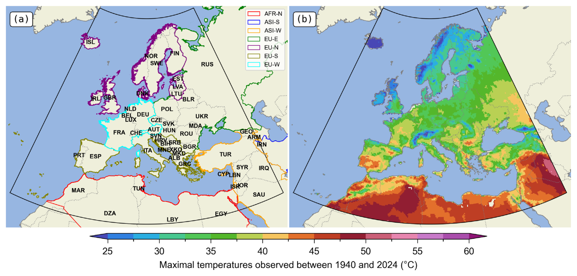
Figure 1 The European domain of this study, stretching from 22° W to 45.5° E, and from 26.5 to 72.5° N, here delimited by the black box. (a) The ISO-3166-1 codes of the countries in the domain have been added (see Table S1). The colored areas follow the UNSD (2020) M49 norm. (b) Maximum temperature observed (ERA5) between 1940 and 2024.

The paper is organized as follows. In Sect. 2, we present the data used: observations, climate models, and the variables we derive from them. In Sect. 3, the methodology is presented, using extreme temperatures at the Paris location (France) as an example. We also analyse the improvements of the new method compared to the case where the scenarios are estimated independently of each other. Section 4 describes the new code, how it is used and what is implemented. Section 5 then looks at current and future maxima over Europe, using a method derived from attribution. Finally, conclusions and perspectives are provided in Sect. 6.

2 Data used

2.1 Observations

We use the “European Reanalysis of the Atmosphere, version 5” data (ERA5 Hersbach et al., 2020) to characterize the historical observation-based extremes, and in the following, ERA5 will be referred to as “observations”. This atmospheric reanalysis combines data from weather forecasting model with observations using assimilation to produce a large number of atmospheric variables. The ERA5 reanalysis provides variables by pressure level at hourly time steps, with surface values calculated by interpolating between the lowest model level and the Earth's surface, taking account of the atmospheric conditions (https://cds.climate.copernicus.eu/datasets/reanalysis-era5-land-timeseries, last access: 19 March 2026). Note that ERA5 is a dataset that may be biased compared to actual observations, particularly for extreme events. Figure S1 in the Supplement shows the difference compared to E-OBS (Cornes et al., 2018) – which is constructed by spatially interpolating surface observations – on average (Fig. S1a) and at maximum (Fig. S1b). The mean bias varies from 1 to 2 K, but locally can grow up to more than 10 K, particularly over North Africa. Despite such well-known limitations, ERA5 has decisive advantages in our context: global coverage (E-OBS is only available for Europe) for the entire time period, with some spatial consistency.

From this dataset, we retain temperatures over our European zone, aggregated on a daily time step, taking daily maxima between 00:00 and 23:00 (UTC), from 1940 to 2024, at the spatial resolution 0.25°. We only retain the land grid points (∼52 % of 185×271 = 50 135 grid points), see Fig. 1a (the Fig. 1b is used in the Sect. 5).

Let us now take a look at how the variable representing a heatwave is constructed for each ERA5 grid point. Starting with daily maximum temperatures (TX), to account for a heatwave extending over several days, we work with the annual maximum of the 3 d moving average, noted TX3x. In general, mortality increases sharply with the duration of heatwaves (D'Ippoliti et al., 2010), and a duration of three days allows us to capture this effect. To illustrate our methodology we zoom over the location of Paris (France). The bias of this time series compared to E-OBS has been represented on the Fig. S1c–d.

In the statistical method used, changes in extremes are assumed to scale with global or regional average temperature – which is used as a covariate. Changes in these spatially averaged temperatures are assumed to capture the response to external forcings. The temperature over Europe will be taken from HadCRUT5 (Morice et al., 2021; Osborn et al., 2021), available from 1850 to the present day. We have chosen to use GISTEMP (Lenssen et al., 2019) for the global temperature.

2.2 Climate models used in this study

Global Climate Models (GCMs) from the Climate Model Intercomparison Project phase 6 (CMIP6 Eyring et al., 2016) simulate climate evolution on a global scale, with a spatial resolution of the order of 100 to 200 km. The simulations feed into numerous scientific projects to understand physical mechanisms, evaluate models, lead multidisciplinary impact studies and serve as a reference for IPCC reports (see, e.g., AR6 reports IPCC, 2021, 2022a, b).

These simulations consist of a historical part, covering the period from 1850 to 2014, and several future emission scenarios ranging from 2015 to 2100. These scenarios are called Shared Socio-economic Pathways (SSP O'Neill et al., 2014; van Vuuren et al., 2014; O'Neill et al., 2016), and describe climate evolution under assumptions of socio-economic evolution of human societies. Four scenarios will be used in this study, describing four levels of warming: the SSP1-2.6 (+1.8 K by the end of the century with respect to 1850/1900 period), the SSP2-4.5 (+2.8 K), the SSP3-7.0 (+4.1 K) and the SSP5-8.5 (+5 K) see, e.g. Ribes et al. (2021).

Lee et al. (2020)Semmler et al. (2018)Wu et al. (2019)Rong et al. (2018)Pu et al. (2020)Swart et al. (2019)Virgin et al. (2021)Lovato et al. (2021)Voldoire et al. (2019)Séférian et al. (2019)Ziehn et al. (2020)Dix et al. (2019)EC-Earth (2019a)EC-Earth (2019b)EC-Earth (2020)Volodin et al. (2018)Volodin et al. (2019)Boucher et al. (2020)Hajima et al. (2019)Tatebe and Watanabe (2018)Good et al. (2019)Mauritsen et al. (2019)Maher et al. (2019)Mauritsen and Roeckner (2020)Yukimoto et al. (2019)Seland et al. (2020)Seland et al. (2020)Bentsen et al. (2019)Krasting et al. (2018)

Table 1 List of CMIP6 models used. The value is the number of members for each scenarios.

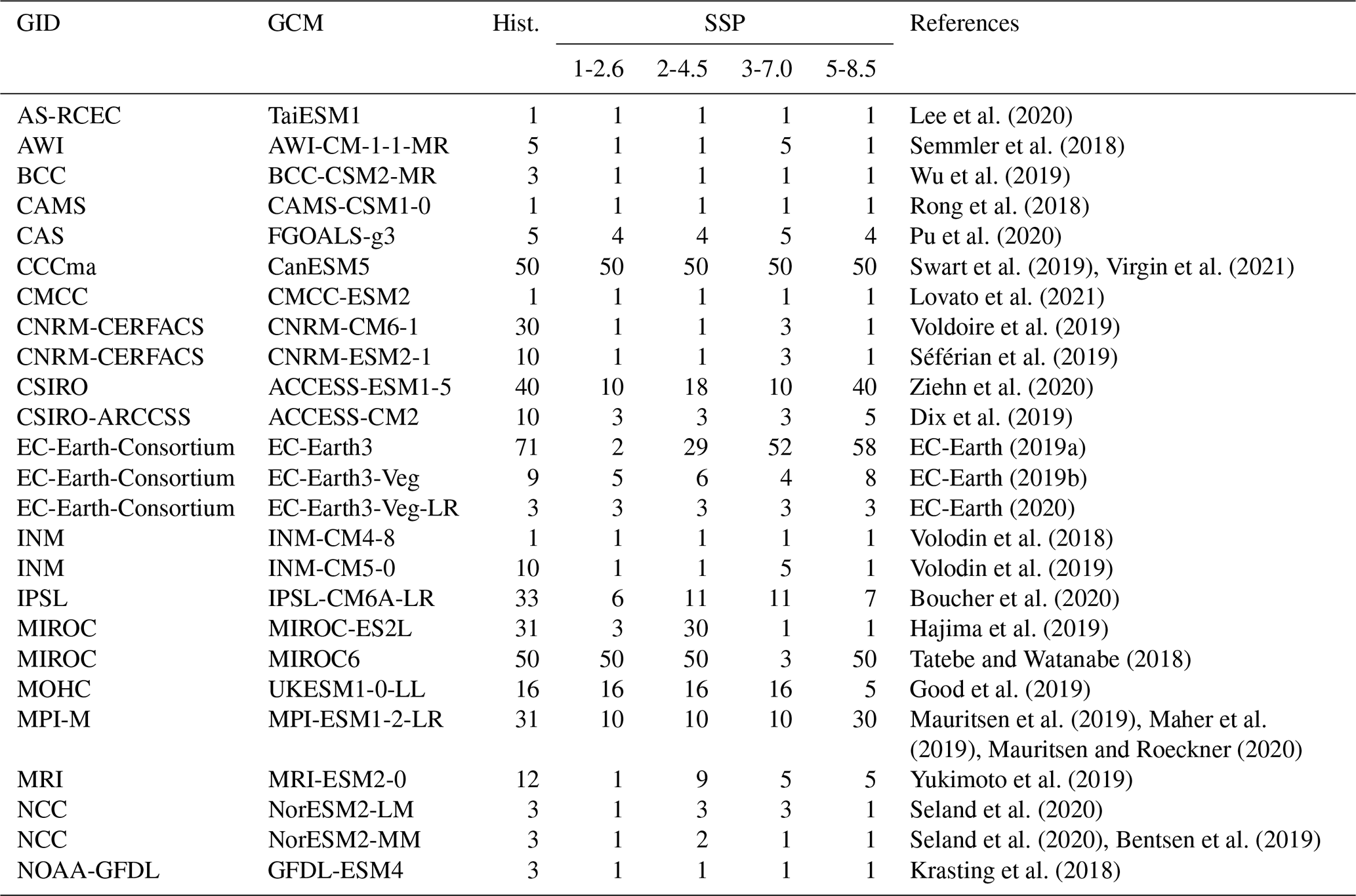
For each model (see Table 1) we take the same variables as for the observations: TX3x on each European grid point, mean annual temperature over Europe, and over the world. These variables cover the period from 1850 to 2100, thus including the historical part as well as the future projections of the four SSPs scenarios described above.

3 Methodology

The aim of this section is to calculate the statistical parameters (of the law of extremes and covariates, but this could be more general) describing these variables, based on global and regional average temperatures and local extremes (for several simulations from climate models and observations). The method we will present here uses a Bayesian approach, where we first seek to construct a prior distribution of reality (using climate models), which we then constrain using observations, defining the posterior distribution. A key point of this approach is that the prior describes a much longer period than the one observed – typically 1850–2100 for climate models versus 1940–2024 for observations – which allows the construction of a posterior over a period where observations are absent.

The Sect. 3.1 will present the statistical model. The inference method is described in Sect. 3.2 and illustrated with a concrete example in Sect. 3.3. The Sect. 3.4 will discuss the benefits of using or not using several climate scenarios simultaneously.

3.1 Definition of the statistical model

The aim of ANKIALE is to enable the inference of a statistical model describing a climate variable (such as the annual maximum temperature) from either a climate model or observations (or similar product, such as reanalyses). The inference strategy, developed by Ribes et al. (2020) in the case of a normal distribution, then by Robin and Ribes (2020a) in the case of extremes, is based on a frequency analysis for climate models and a Bayesian analysis for observations. This difference in treatment stems from the idea, already exploited by Ribes et al. (2017), that a set of climate models can be used to construct an approximation of reality, called a prior, and that observations can be used to constrain this prior to what has been observed, allowing the construction of what is called the posterior. This posterior therefore incorporates information from climate models, constrained in such a way as to be made compatible with observations.

Formally, we have a climate variable T_t that follows a parametric probability distribution, whose parameters can be summarised in a vector θ. This vector θ can incorporate parameters that control a large number of elements, such as those parameterising the intensity of external forcings that apply at a time t, as well as the parameters of the underlying distribution. In this paper, we take as an example the annual maximum temperatures (over 3 d), which are assumed to follow a GEV (Generalised Extreme Value) distribution (see Appendix A), which is a standard choice in the literature for this variable (see, e.g., Pinto et al., 2024; Zachariah et al., 2023b; Barnes et al., 2023; van Oldenborgh et al., 2019). It should be noted that our method can be adapted to other types of statistical models (such as Gaussian models). This distribution has three parameters: μ (location parameter, similar to the mean), σ (scale parameter, similar to the standard deviation) and ξ (shape parameter, controlling whether or not the extremes are bounded). The first two of these parameters are assumed to evolve over time scaling with a covariable X_t, which is representative of a mean climate change.

A statistical model typically used in attribution, as for example by Philip et al. (2020) or Otto et al. (2024) (assuming X_t is known), is given by:

$$\begin{array}{}\text{(1)}& \left\{\begin{array}{ll}{T}_t& \sim \mathrm{GEV}({\mathit{\mu }}_t,{\mathit{\sigma }}_t,{\mathit{\xi }}_t)\\ {\mathit{\mu }}_t& ={\mathit{\mu }}_{\mathrm{0}}+{\mathit{\mu }}_{\mathrm{1}}{X}_t\\ \log {\mathit{\sigma }}_t& \equiv {\mathit{\sigma }}_{\mathrm{0}}\\ {\mathit{\xi }}_t& \equiv {\mathit{\xi }}_{\mathrm{0}}\end{array}\right.\end{array}$$

The idea is that climate change modifies the location parameter μ_t over time (which is similar to the increase of the mean), but that the variability and shape of the extremes remain unchanged. The indicator describing climate change X_t is generally given by a smoothing of the global temperature (e.g. a 15-year moving average). Then, the vector θ of the parameters of our statistical model can be written:

$$\begin{array}{}\text{(2)}& \mathit{\theta }:=({\mathit{\mu }}_{\mathrm{0}},{\mathit{\mu }}_{\mathrm{1}},{\mathit{\sigma }}_{\mathrm{0}},{\mathit{\xi }}_{\mathrm{0}}).\end{array}$$

θ can be estimated directly from observations or from climate simulations using maximum likelihood. Confidence intervals on θ are constructed using bootstrap. In this model, uncertainty on the climate change indicator X_t is not taken into account.

One further difficulty for practical application to climate data, is that the covariate X_t representing the response to climate change, is not fully well-known in general, and brings it's own uncertainty. This also applies to the breakdown between the response to natural forcings $X_t^{\mathrm{N}}$ and the response to anthropogenic forcings $X_t^{\mathrm{A}}$. One possibility to include this additional uncertainty in our statistical model is to include X_t on the model parameters, thus extending the vector θ. This type of statistical model has been studied by Ribes et al. (2020) for the normal distribution and Robin and Ribes (2020a) for the GEV distribution, including a dependence on X_t for the scale parameter σ_t. It is written as follows:

$$\begin{array}{}\text{(3)}& \left\{\begin{array}{ll}{T}_t& \sim \mathrm{GEV}({\mathit{\mu }}_t,{\mathit{\sigma }}_t,{\mathit{\xi }}_t)\\ {\mathit{\mu }}_t& ={\mathit{\mu }}_{\mathrm{0}}+{\mathit{\mu }}_{\mathrm{1}}{X}_t\\ \log {\mathit{\sigma }}_t& ={\mathit{\sigma }}_{\mathrm{0}}+{\mathit{\sigma }}_{\mathrm{1}}{X}_t\\ {\mathit{\xi }}_t& \equiv {\mathit{\xi }}_{\mathrm{0}}\\ X_t& =X^{\mathrm{0}}+X_t^{\mathrm{N}}+X_t^{\mathrm{A}}\end{array}\right.\end{array}$$

For this statistical model, θ therefore takes the following form:

$$\begin{array}{}\text{(4)}& \mathit{\theta }:=(X^{\mathrm{0}},X_t^{\mathrm{N}},X_t^{\mathrm{A}},{\mathit{\mu }}_{\mathrm{0}},{\mathit{\mu }}_{\mathrm{1}},{\mathit{\sigma }}_{\mathrm{0}},{\mathit{\xi }}_{\mathrm{0}}).\end{array}$$

This statistical model has several limitations:

• It does not incorporate the work of Qasmi and Ribes (2022), who worked on how to simultaneously account for global and regional covariates (which is important, for example, when the regional response differs significantly from the global response, due to aerosols).

• Only one scenario for the future period can be used at a time, which may lead to different estimates for the historical period;

• The parameters X⁰ (a constant) and $X_t^{\mathrm{N}}$, which model the response to natural forcings, should not depend on the scenario.

In ANKIALE, we propose using a statistical model that meets the following constraints:

• The covariate can be global (denoted $X_t^{\mathrm{G}}$) and / or regional (denoted $X_t^{\mathrm{R}}$);

• Allow for the simultaneous consideration of multiple future SSP scenarios;

• The response to natural forcings do not depend on the SSP (or historical) scenario.

Starting from several climate variables $T_t^{\mathrm{SSP}}$, $\mathrm{SSP}\in \mathit{\{}{\mathrm{SSP}}_{\mathrm{1}},\mathrm{\dots },{\mathrm{SSP}}_{N_{\mathrm{SSP}}}\mathit{\}}$ (the term SSP here referring to one of the possible future scenarios, but the time series include also the historical period), this model can be written as:

$$\begin{array}{}\text{(5)}& \left\{\begin{array}{ll}{T}_t^{{\mathrm{SSP}}_{\mathrm{1}}}& \sim \mathrm{GEV}\left({\mathit{\mu }}_t^{{\mathrm{SSP}}_{\mathrm{1}}},{\mathit{\sigma }}_t^{{\mathrm{SSP}}_{\mathrm{1}}},{\mathit{\xi }}_t^{{\mathrm{SSP}}_{\mathrm{1}}}\right)\\ {\mathit{\mu }}_t^{{\mathrm{SSP}}_{\mathrm{1}}}& ={\mathit{\mu }}_{\mathrm{0}}+X_t^{R,{\mathrm{SSP}}_{\mathrm{1}}}{\mathit{\mu }}_{\mathrm{1}}\\ \log {\mathit{\sigma }}_t^{{\mathrm{SSP}}_{\mathrm{1}}}& ={\mathit{\sigma }}_{\mathrm{0}}+X_t^{R,{\mathrm{SSP}}_{\mathrm{1}}}{\mathit{\sigma }}_{\mathrm{1}}\\ {\mathit{\xi }}_t^{{\mathrm{SSP}}_{\mathrm{1}}}& \equiv {\mathit{\xi }}_{\mathrm{0}}\\ X_t^{R,{\mathrm{SSP}}_{\mathrm{1}}}& =X^{R,\mathrm{0}}+X_t^{R,\mathrm{N}}+X_t^{R,{\mathrm{SSP}}_{\mathrm{1}},\mathrm{A}}\\ X_t^{G,{\mathrm{SSP}}_{\mathrm{1}}}& =X^{G,\mathrm{0}}+X_t^{G,\mathrm{N}}+X_t^{G,{\mathrm{SSP}}_{\mathrm{1}},\mathrm{A}}\\ \mathrm{⋮}& =\mathrm{⋮}\\ T_t^{{\mathrm{SSP}}_{N_{\mathrm{SSP}}}}& \sim \mathrm{GEV}\left({\mathit{\mu }}_t^{{\mathrm{SSP}}_{N_{\mathrm{SSP}}}},{\mathit{\sigma }}_t^{{\mathrm{SSP}}_{N_{\mathrm{SSP}}}},{\mathit{\xi }}_t^{{\mathrm{SSP}}_{N_{\mathrm{SSP}}}}\right)\\ {\mathit{\mu }}_t^{{\mathrm{SSP}}_{N_{\mathrm{SSP}}}}& ={\mathit{\mu }}_{\mathrm{0}}+X_t^{R,{\mathrm{SSP}}_{N_{\mathrm{SSP}}}}{\mathit{\mu }}_{\mathrm{1}}\\ \log {\mathit{\sigma }}_t^{{\mathrm{SSP}}_{N_{\mathrm{SSP}}}}& ={\mathit{\sigma }}_{\mathrm{0}}+X_t^{R,{\mathrm{SSP}}_{N_{\mathrm{SSP}}}}{\mathit{\sigma }}_{\mathrm{1}}\\ {\mathit{\xi }}_t^{{\mathrm{SSP}}_{N_{\mathrm{SSP}}}}& \equiv {\mathit{\xi }}_{\mathrm{0}}\\ X_t^{R,{\mathrm{SSP}}_{N_{\mathrm{SSP}}}}& =X^{R,\mathrm{0}}+X_t^{R,\mathrm{N}}+X_t^{R,{\mathrm{SSP}}_{N_{\mathrm{SSP}}},\mathrm{A}}\\ X_t^{G,{\mathrm{SSP}}_{N_{\mathrm{SSP}}}}& =X^{G,\mathrm{0}}+X_t^{G,\mathrm{N}}+X_t^{G,{\mathrm{SSP}}_{N_{\mathrm{SSP}}},\mathrm{A}}\end{array}\right.\end{array}$$

This model appears to be an extension of the one defined by Eq. (1) for each of the SSP scenarios, while incorporating the response to external forcings on σ_t in addition to μ_t. The two variables $X_t^{\mathrm{R},\mathrm{SSP}}$ and $X_t^{\mathrm{G},\mathrm{SSP}}$ correspond respectively to the Regional and Global forcings of historical and each SSP scenario. They are both decomposed as the sum of a constant (X^R,0 and X^G,0, respectively), a response to Natural forcings ($X_t^{\mathrm{R},\mathrm{N}}$ and $X_t^{\mathrm{G},\mathrm{N}}$, respectively) and a response to Anthropogenic forcings ($X_t^{\mathrm{R},\mathrm{SSP},\mathrm{A}}$ and $X_t^{\mathrm{G},\mathrm{SSP},\mathrm{A}}$, respectively), see Sect. S1.1 in the Supplement for the exact mathematical description and how the decomposition is performed. The vector θ, equivalent to Eq. (2), and obtained after including all these terms, is given by:

$$\begin{array}{}\text{(6)}& \begin{array}{rl}\mathit{\theta }:=& (X^{R,\mathrm{0}},X_t^{\mathrm{R},\mathrm{N}},X_t^{\mathrm{R},{\mathrm{SSP}}_{\mathrm{1}},\mathrm{A}},\mathrm{\dots },X_t^{\mathrm{R},{\mathrm{SSP}}_{N_{\mathrm{SSP}}},\mathrm{A}},\\ & X^{\mathrm{G},\mathrm{0}},X_t^{\mathrm{G},\mathrm{N}},X_t^{\mathrm{G},{\mathrm{SSP}}_{\mathrm{1}},\mathrm{A}},\mathrm{\dots },X_t^{\mathrm{G},{\mathrm{SSP}}_{N_{\mathrm{SSP}}},\mathrm{A}},\\ & {\mathit{\mu }}_{\mathrm{0}},{\mathit{\mu }}_{\mathrm{1}},{\mathit{\sigma }}_{\mathrm{0}},{\mathit{\sigma }}_{\mathrm{1}},{\mathit{\xi }}_{\mathrm{0}}).\end{array}\end{array}$$

In this statistical model, only anthropogenic terms depend on the historical and SSP scenario. Compared to the model defined in Eq. (1), the scale parameter ${\mathit{\sigma }}_t^{\mathrm{SSP}}$ depends on $X_t^{\mathrm{R},\mathrm{SSP}}$ and is therefore no longer constant over time. Note that the parameters ${\mathit{\mu }}_t^{\mathrm{SSP}}$ and ${\mathit{\sigma }}_t^{\mathrm{SSP}}$ depend directly only on the regional forcings $X_t^{\mathrm{R},\mathrm{SSP}}$. They depend indirectly on the global forcings $X_t^{\mathrm{G},\mathrm{SSP}}$ through the knowledge of the dependence between the parameters in the vector θ (a vector that integrates all the information in the statistical model). This makes it possible to link global warming to local events. We also assume that the coefficients of the GEV distribution μ₀, μ₁, σ₀, σ₁ and ξ₀ are independent of external forcings. This model is flexible and allows the underlying distribution to be easily modified. For example, it is possible to replace the GEV law with a Gaussian law (this statistical model is also proposed in ANKIALE). Other statistical models (with possibly others probability distributions), not necessarily implemented immediately, are proposed in Sect. S2.

In the following, in order to facilitate notation, we will break down θ as follows:

$$\left\{\begin{array}{ll}\mathit{\theta }& :=({\mathit{\theta }}^{\mathrm{R}},{\mathit{\theta }}^{\mathrm{G}},{\mathit{\theta }}^{\mathrm{GEV}}),\\ {\mathit{\theta }}^{\mathrm{R}}& :=\left(X^{\mathrm{R},\mathrm{0}},X_t^{\mathrm{R},\mathrm{N}},X_t^{\mathrm{R},{\mathrm{SSP}}_{\mathrm{1}},\mathrm{A}},\mathrm{\dots },X_t^{\mathrm{R},{\mathrm{SSP}}_{N_{\mathrm{SSP}}},\mathrm{A}}\right),\\ {\mathit{\theta }}^{\mathrm{G}}& :=\left(X^{\mathrm{G},\mathrm{0}},X_t^{\mathrm{G},\mathrm{N}},X_t^{\mathrm{G},{\mathrm{SSP}}_{\mathrm{1}},\mathrm{A}},\mathrm{\dots },X_t^{\mathrm{G},{\mathrm{SSP}}_{N_{\mathrm{SSP}}},\mathrm{A}}\right),\\ {\mathit{\theta }}^{\mathrm{GEV}}& :=({\mathit{\mu }}_{\mathrm{0}},{\mathit{\mu }}_{\mathrm{1}},{\mathit{\sigma }}_{\mathrm{0}},{\mathit{\sigma }}_{\mathrm{1}},{\mathit{\xi }}_{\mathrm{0}}).\end{array}\right.$$

3.2 Estimation strategy

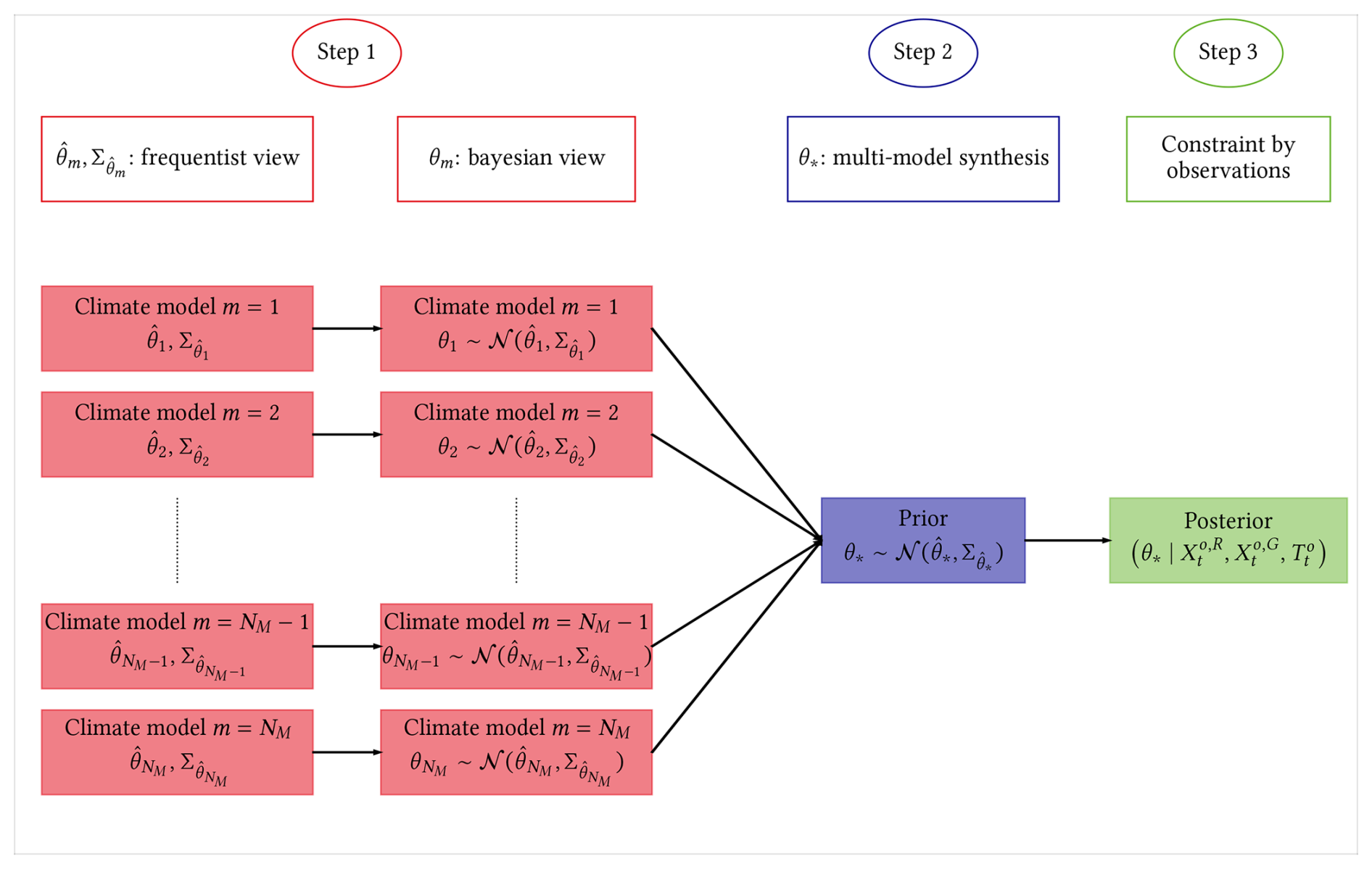
As mentioned at the beginning of the previous section, estimation in ANKIALE is carried out in three steps, which are summarised in Fig. 2. This strategy can be summarised as follows:

1. Inference in climate models. For each climate model $m=\mathrm{1},\mathrm{\dots },N_M$, let θ_m be the value of θ for model m. We derive an estimate ${\widehat{\mathit{\theta }}}_m$ of θ_m, as well as the covariance matrix describing the estimation error, denoted ${\mathbf{\Sigma }}_{{\widehat{\mathit{\theta }}}_m}$, using a standard frequentist approach. Details are given in Appendix B1.

2. Construction of the multi-model synthesis. At this stage, we switch to a Bayesian approach. The vector θ_m is now considered a random variable for each climate model $m=\mathrm{1},\mathrm{\dots },N_M$, for which we seek to estimate the probability distribution ℙ(θ_m). Since we have an estimate ${\widehat{\mathit{\theta }}}_m$ and a covariance matrix ${\mathbf{\Sigma }}_{{\widehat{\mathit{\theta }}}_m}$, the multivariate normal distribution is the natural choice:

   $${\mathit{\theta }}_m\sim \mathbb{P}\left({\mathit{\theta }}_m\right):=\mathcal{N}({\widehat{\mathit{\theta }}}_m,{\mathbf{\Sigma }}_{{\widehat{\mathit{\theta }}}_m}).$$

   The multi-model synthesis, denoted θ_∗, follows also a multivariate normale distribution:

   $$\begin{array}{}\text{(7)}& {\mathit{\theta }}_{\ast }\sim \mathbb{P}\left({\mathit{\theta }}_{\ast }\right):=\mathcal{N}({\widehat{\mathit{\theta }}}_{\ast },{\mathbf{\Sigma }}_{{\widehat{\mathit{\theta }}}_{\ast }}).\end{array}$$

   The mean ${\widehat{\mathit{\theta }}}_{\ast }$ is just given by the multi-model mean, but the covariance matrix ${\mathbf{\Sigma }}_{{\widehat{\mathit{\theta }}}_{\ast }}$ is more complex, and takes into account of intra and inter model uncertainy. Details are given in the Appendix B2. It is this random variable that will serve as our prior in the following.

3. Derivation of the posterior with observations. Knowing the observations $X_t^{\mathrm{o},\mathrm{R}}$, $X_t^{\mathrm{o},\mathrm{G}}$ and $T_t^{\mathrm{o}}$ (regional, global and extreme average temperatures, defined in Sect. 2.1) and the prior θ_∗, the aim here is to estimate the distribution $\mathbb{P}\left[{\mathit{\theta }}_{\ast }\right|(X_t^{\mathrm{o},\mathrm{R}},X_t^{\mathrm{o},\mathrm{G}},T_t^{\mathrm{o}})]$, i.e. the distribution of θ_∗ knowing what has been observed. This conditional distribution thus incorporates information from climate models (through the prior) while being compatible with observations (via the conditioning). The derivation of the posterior from the prior is detailed in Appendix B3.

We will now illustrate these different steps using temperatures in Paris.

Figure 2 Illustration of the procedure for estimating the parameter vector θ, defined by Eqs. (5) and (6).

3.3 Illustration with the TX3x at Paris

In this section, we illustrate our procedure using the annual maximum daily temperatures over 3 d (T_t:=TX3x, with a slight abuse of notation in the omission of time in TX3x). According to the block-maxima theorem (see, e.g., Coles, 2001), we assume that the random variable TX3x follows a GEV distribution.

3.3.1 Step 1: Estimations for the climate models

The first step is to estimate ${\widehat{\mathit{\theta }}}_m$ and ${\mathbf{\Sigma }}_{{\widehat{\mathit{\theta }}}_m}$ for the different climate models m. We can see the result for the climate model IPSL-CM6A-LR (Boucher et al., 2020), over the historical period followed by the SSP5-8.5 scenario, in Fig. 3.

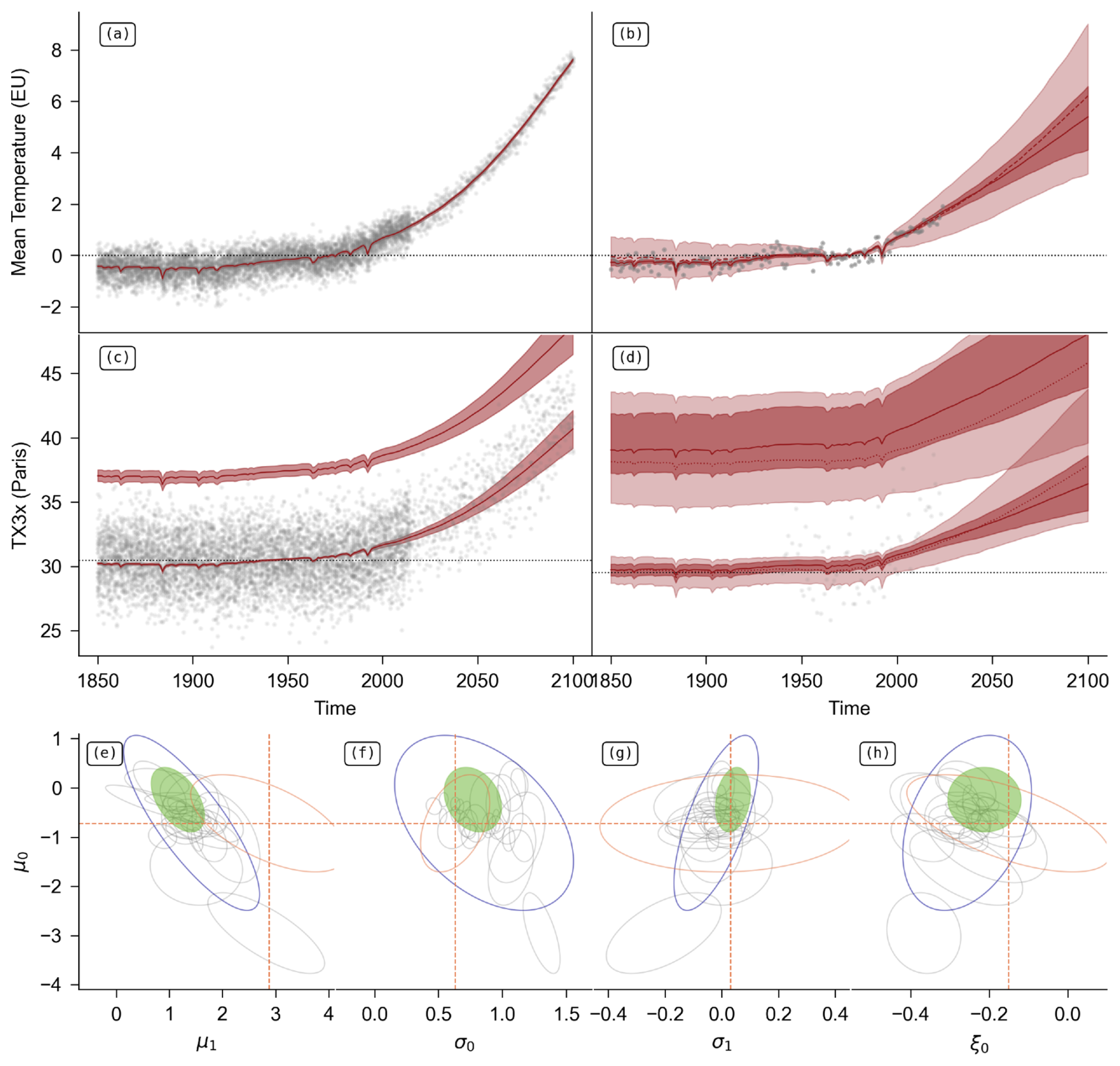
Figure 3 Illustration of the methodology described in Sect. 3. (a) Mean forcing (red line) for the Europe covariate of the IPSL model (grey dots), for the SSP5-8.5 scenario. The 95 % confidence interval is given by the solid red area. (b) Multi-model synthesis (light red) and posterior (dark red) after constraint by observations (in grey) for the Europe covariate, for the SSP5-8.5 scenario. (c) TX3x series in Paris from the IPSL model (grey dots) for the SSP5-8.5 scenario. The red line passing through the model data is the median, with its 95 % confidence interval (filled area). The red line above the data is the upper bound, also with its 95 % confidence interval. (d) Same as (c), for the prior (multi-model synthesis, in light red) and the posterior (constrained by observations, in dark red). The grey dots are observations from ERA5. (e) Parameters μ₁ as a function of μ₀ for climate models (in grey), the multi-model synthesis (in blue), the posterior after constraint (in green), and the direct estimate from observations (orange). The ellipses represent the 95 % confidence interval for the pair of parameters. The parameters are those estimated in Paris. (f) Same as (e), for σ₀ as a function of μ₀. (g) Same as (e), for σ₁ as a function de μ₀. (h) Same as (e), for ξ₀ as a function de μ₀.

In Fig. 3a, showing the regional covariate over Europe, the values of the 33 members of the IPSL model are shown in grey, and the estimate of $X_t^{\mathrm{R},m}$ in red, with the 95 % confidence interval. The covariate appears to pass through the centre of the data set (as expected), with dips caused by volcanic activity. In Fig. 3c, showing the variable TX3x, the values of the 33 members of the IPSL model are shown in grey. The red line passing through the data is the median, with its 95 % interval. The red line above the data set is the upper bound (see Appendix A), with its 95 % interval.

We have also represented the estimates of ${\widehat{\mathit{\theta }}}_m^{\mathrm{GEV}}$ as pairs between μ₀ and the other parameters μ₁, σ₀, σ₁ and ξ₀, in Fig. 3e–h. These estimates are represented with the ellipse defined by the covariance matrix ${\mathbf{\Sigma }}_{{\widehat{\mathit{\theta }}}_m}$ at the 95 % level, in grey. We can see that the parameter μ₁, which drives the average trend of extremes, ranges from a value of almost zero in some models to a factor of 4. The equivalent parameter for scale, σ₁, is centred at 0. The shape parameter ξ₀ is strictly negative regardless of the model, which is typical for temperatures. Note that the model with the lower μ₀, which differs from the other climate models, is the NorESM2-LM model (Norwegian Bentsen et al., 2019).

3.3.2 Step 2: construction of the prior with the multi-model synthesis

The next step is the multi-model synthesis, which is shown in Fig. 3b, d (for the covariable) and Fig. 3e–h (for the GEV parameters).

In Fig. 3b, the regional covariate over Europe is shown in light red. Compared to Fig. 3a, the 95 % confidence interval is much wider, encompassing all climate models. Since we are working with anomalies relative to the 1961–1990 period, the uncertainty is much lower in this period.

Figure 3d shows in light red the median and upper bound of the GEV distribution (see Appendix A for the definitions of the quantile function and the upper bound), with their 95 % confidence intervals. We can see that the intervals are particularly wide compared to those of the IPSL model in Fig. 3c, as they encompass the uncertainty from all climate models. ERA5 observations have been added (grey dots), as well as the average of observations over the period 1961/1990 (black dotted line). The median of the synthesis seems strongly biased compared to the observations, as the confidence interval does not contain the 1961/1990 mean (the median and the mean are quite close for the GEV distribution).

In Fig. 3e–h, the multi-model synthesis is shown in blue. We can see that it encompasses all the parameters from each of the climate models, thus taking into account their uncertainties.

3.3.3 Step 3: derivation of the posterior with observations

The final step is a constraint by the observations, which is shown in Fig. 3b, d (for the covariable) and Fig. 3e–h (for the GEV parameters).

Figure 3b displays the observations in grey and the posterior in dark red for the European covariate. The posterior fits the observations well (modulo natural variability). The 95 % confidence interval appears considerably reduced (from 2° at the beginning of the century to 4° at the end of the century). The posterior is shown in dark red in Fig. 3d. The confidence interval (both for the median and the upper bound) has been considerably reduced compared to the prior (in light red). The median also appears unbiased, with a confidence interval close to the 1961/1990 average for the historical part.

In Fig. 3e–h, the posterior is shown in green. For comparison, we have also added a direct estimate from ERA5 by maximum likelihood in orange: the statistical model of Eq. (1) is inferred (with the addition of σ_t which depends on X_t), and for the covariate X_t we use the posterior of $X_t^R$. Compared to the prior (in blue), the posterior shows a significant reduction in uncertainty. It should also be noted that the posterior is not centred on the prior, but may appear shifted. With the exception of μ₁, the direct estimate of ERA5 appears to be compatible with the prior, albeit with extremely high uncertainty: the parameter ξ₀ may even be positive in this case, allowing for extreme TX3x events with potentially colossal values. Two specific cases stand out:

1. σ₁ shows significant uncertainty in ERA5 (although centred at 0), which is strongly constrained to 0 by Bayesian inference methods.

2. μ₁ also shows significant uncertainty in ERA5, but also significant bias: the values can exceed +4 °C (in the 95 % confidence interval), whereas they do not exceed +2 °C in the posterior (which implies a slope that is twice as small). The explanation lies in the fact that μ₁ in ERA5 is estimated from a very small number of values (the climate change signal is almost imperceptible before the 1990s, as we can see in Fig. 3b). As our approach uses information from models, this parameter is estimated from future scenarios and becomes much less uncertain.

3.4 Contribution of the multi-scenario approach in an attribution context

3.4.1 Analysis through the attribution of the 2019 French heatwave

A new feature of the statistical model developed in Eqs. (5) and (6) is the simultaneous consideration of several scenarios while requiring that the natural part of external forcings be common to the different scenarios. In order to measure the contribution of this approach, we attributed the 2019 heatwave in Paris, which has a Factual Intensity of $I_{\mathrm{2019}}^{\mathrm{F}}:=\mathrm{38.7}$ °C in ERA5. Our statistical model is inferred in five cases:

• A case where four SSP scenarios are used simultaneously, i.e. $\text{SSP}\in \mathit{\{}\text{SSP1-2.6},\text{SSP2-4.5},\text{SSP3-7.0},\text{SSP5-8.5}\mathit{\}}$,

• A case where SSP is only the SSP1-2.6 scenario,

• A case where SSP is only the SSP2-4.5 scenario,

• A case where SSP is only the SSP3-7.0 scenario,

• A case where SSP is only the SSP5-8.5 scenario,

For each of these cases and each scenarios, we calculated the regional covariates Factual $X_t^{\mathrm{F}}$ (with human influence) and Counterfactual $X_t^{\mathrm{C}}$ (natural forcings only) as follows:

$$\left\{\begin{array}{rl}{\displaystyle }{X}_t^{\mathrm{F}}& {\displaystyle }=X^{\mathrm{R},\mathrm{0}}+X_t^{\mathrm{R},\mathrm{N}}+X_t^{\mathrm{R},\mathrm{A}},\\ {\displaystyle }{X}_t^{\mathrm{C}}& {\displaystyle }=X^{\mathrm{R},\mathrm{0}}+X_t^{\mathrm{R},\mathrm{N}}.\end{array}\right.$$

By inserting these two terms into the parameters of locations, scales and shapes of the GEV distribution, survival functions and quantile functions can be calculated in factual and counterfactual worlds. This makes it possible to calculate the probability of exceeding the threshold $I_{\mathrm{2019}}^{\mathrm{F}}$ each year t, in factual and counterfactual worlds. Using the equations recalled in Appendix A, for a GEV distribution, the probability in the factual world $p_t^{\mathrm{F}}$ (resp. counterfactual $p_t^{\mathrm{C}}$) that the TX3x exceeds $I_{\mathrm{2019}}^{\mathrm{F}}$ in year t, and the intensity $I_t^{\mathrm{F}}$ (or $I_t^{\mathrm{C}}$) of an event with the same probability (as 2019) are given by:

$$\begin{array}{}\text{(8)}& \begin{array}{rl}& \left\{\begin{array}{ll}{p}_t^{\mathrm{F}}& :=\mathrm{1}-F_{\mathrm{GEV}}(I_{\mathrm{2019}}^{\mathrm{F}};{\mathit{\mu }}_t^{\mathrm{F}},{\mathit{\sigma }}_t^{\mathrm{F}},{\mathit{\xi }}_t^{\mathrm{F}})\\ I_t^{\mathrm{F}}& :={\mathcal{Q}}_{\mathrm{GEV}}(\mathrm{1}-p_{\mathrm{2019}}^{\mathrm{F}};{\mathit{\mu }}_t^{\mathrm{F}},{\mathit{\sigma }}_t^{\mathrm{F}},{\mathit{\xi }}_t^{\mathrm{F}})\\ {\mathit{\mu }}_t^{\mathrm{F}}& ={\mathit{\mu }}_{\mathrm{0}}+{\mathit{\mu }}_{\mathrm{1}}{X}_t^{\mathrm{F}}\\ \log {\mathit{\sigma }}_t^{\mathrm{F}}& ={\mathit{\sigma }}_{\mathrm{0}}+{\mathit{\sigma }}_{\mathrm{1}}{X}_t^{\mathrm{F}}\\ {\mathit{\xi }}_t^{\mathrm{F}}& \equiv {\mathit{\xi }}_{\mathrm{0}}\end{array}\right.,\\ & \left\{\begin{array}{ll}{p}_t^{\mathrm{C}}& :=\mathrm{1}-F_{\mathrm{GEV}}(I_{\mathrm{2019}}^{\mathrm{F}};{\mathit{\mu }}_t^{\mathrm{C}},{\mathit{\sigma }}_t^{\mathrm{C}},{\mathit{\xi }}_t^{\mathrm{C}})\\ I_t^{\mathrm{C}}& :={\mathcal{Q}}_{\mathrm{GEV}}(\mathrm{1}-p_{\mathrm{2019}}^{\mathrm{F}};{\mathit{\mu }}_t^{\mathrm{C}},{\mathit{\sigma }}_t^{\mathrm{C}},{\mathit{\xi }}_t^{\mathrm{C}})\\ {\mathit{\mu }}_t^{\mathrm{C}}& ={\mathit{\mu }}_{\mathrm{0}}+{\mathit{\mu }}_{\mathrm{1}}{X}_t^{\mathrm{C}}\\ \log {\mathit{\sigma }}_t^{\mathrm{C}}& ={\mathit{\sigma }}_{\mathrm{0}}+{\mathit{\sigma }}_{\mathrm{1}}{X}_t^{\mathrm{C}}\\ {\mathit{\xi }}_t^{\mathrm{C}}& \equiv {\mathit{\xi }}_{\mathrm{0}}\end{array}\right..\end{array}\end{array}$$

These formulas can be used to construct the classic indicators of change in intensity ($\mathrm{\Delta }{I}_t:=I_t^{\mathrm{F}}-I_t^{\mathrm{C}}$) and probability ratio (${\mathrm{PR}}_t:=p_t^{\mathrm{F}}/p_t^{\mathrm{C}}$). Note that the definition of $I_t^{\mathrm{F}}$ naturally implies that $I_{t=\mathrm{2019}}^{\mathrm{F}}=I_{\mathrm{2019}}^{\mathrm{F}}$ (the left term is the value of a function, while the term on the right is the value of the intensity of the event, defined from the data).

We will use these six indicators $p_t^{\mathrm{F}}$, $p_t^{\mathrm{C}}$, $I_t^{\mathrm{F}}$, $I_t^{\mathrm{C}}$, $X_t^{\mathrm{F}}$ and $X_t^{\mathrm{C}}$, calculated in cases where scenarios are inferred together or separately, in order to analyse the contribution of our approach. To do this, we performed 5000 samples of each of these indicators according to the law defined by the posterior, and we constructed quantile-quantile diagrams between the different scenarios for the years 1850, 1884, 1950, 1992, 2050 and 2100. The last two years are only available for counterfactual variables, as the factual variables show divergences from the scenarios. The years 1884 and 1992 correspond to two minima in natural forcings (see Fig. S2). If the scenarios are analysed separately, the counterfactual worlds associated with each scenario may be different, and the quantile-quantile plots will show deviations. Our approach is expected to greatly reduce these differences. The quantile-quantile plots are shown in Fig. 4. For each panel and each colour (blue for simultaneous scenarios, red for independent scenarios), we have six QQ plots (all possible pairs for four scenarios).

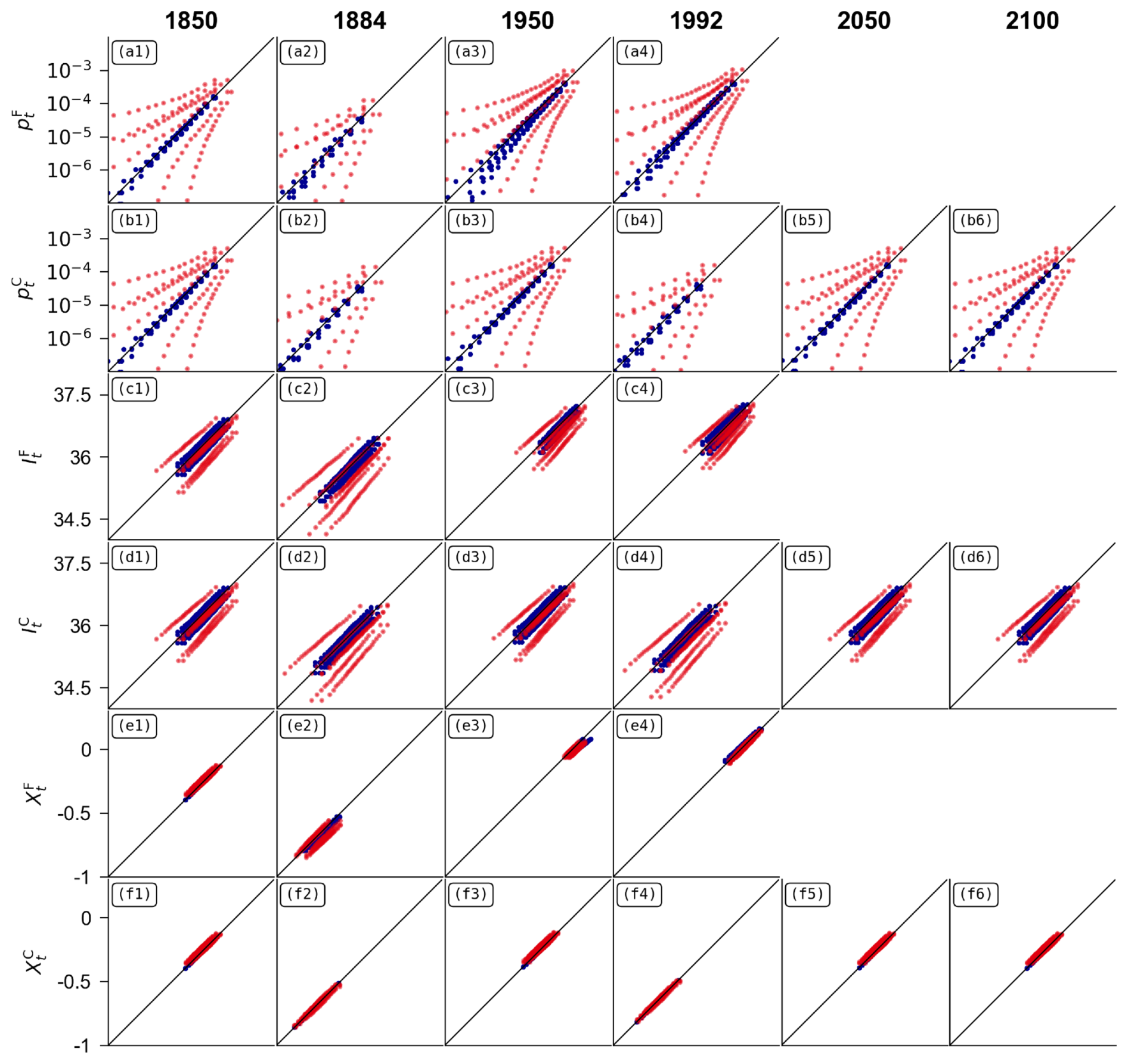
Figure 4 Quantile-quantile plot between 5000 draws of the indicators $p_t^{\mathrm{F}}$, $p_t^{\mathrm{C}}$, $I_t^{\mathrm{F}}$, $I_t^{\mathrm{C}}$, $X_t^{\mathrm{F}}$ and $X_t^{\mathrm{C}}$, for the years 1850, 1884, 1950, 1992, 2050, and 2100. The x-axis is the same as the y-axis (hence the presence of the diagonal), which is given in the first column. These indicators are constructed based on the attribution of the 2019 heatwave for the variable TX3x for all the scenarios. In red, the quantile-quantile plot is constructed when the attribution is performed considering the SSP scenarios independently. In blue, the quantile-quantile plot is constructed when the attribution is performed considering the SSP scenarios simultaneously. The years 1884 and 1992 correspond to minima in natural forcings (see Fig. S2).

Let us begin with the probabilities $p_t^{\mathrm{F}}$ and $p_t^{\mathrm{C}}$, lines a and b. In the counterfactual world in the case of joint scenarios (blue values), the quantile-quantile diagrams are almost perfectly aligned on the diagonal, showing that the data distributions of the four scenarios are indeed the same. In the case where the scenarios are handled separately (in red) in the counterfactual world, the values are much more dispersed, showing a significant deviation between the different counterfactuals. In the factual world, the results are similar in 1850 and 1884, but the dispersion around the diagonal of the dependent case is greater in 1950 and 1992, due to the influence of the scenarios. The scenarios are not supposed to intervene at these points in time (in CMIP6, the SSPs begin in 2015), but inference on the complete series makes the smoothed values of the historical part partially dependent on the values of the part where the scenarios intervene.

Let us continue with the intensities in the factual and counterfactual worlds, lines c and d. The results are the same as for probabilities, with the dispersion appearing greater for probabilities due to the log scale.

Let us conclude with the two factual and counterfactual regional covariates, lines e and f. The results are similar to the intensities and the probabilities.

3.4.2 Influence of the intensity of the event

During an attribution exercise, the analysed event may have a probability of zero (particularly in the counterfactual world), even within the entire confidence interval. This phenomenon may lead to the appearance of ceiling or floor values through the propagation of this 0. In order to quantify the significance of this phenomenon and how the multi-scenario behaves, we propose to perform two attributions, where $I_{\mathrm{2019}}^{\mathrm{F}}$ is defined as the median of the GEV distribution in 2019, and the 99.9 % quantile (value that may pose a problem). We have reproduced Fig. 4 for these two events in Figs. S3 and S4.

Figure S4, which is in a similar context to the attribution of a very strong event, is equivalent to Fig. 4, showing the same behavior. However, Fig. S3, constructed from a probable event (50 %), shows a smaller difference between factual and counterfactual probabilities. The latter are now also distributed around the diagonal, showing equivalence between the multi-scenario and single-scenario approaches. We therefore conclude that the multi-scenario approach does indeed allow for a more consistent estimation of counterfactual probabilities between scenarios for the most extreme events, but that the contribution is weaker for more common events.

4 ANKIALE: ANalysis of Klimate with bayesian Inference: AppLication to extreme Events

The original method, proposed by Robin and Ribes (2020a), was accompanied by a package written in python (Van Rossum and Drake, 2009) or R (R Core Team, 2024): Non-Stationary Statistics for Extreme Attribution (NSSEA Robin and Ribes, 2020b) to reproduce their results. Although this package can be used for attribution studies, the construction of its non-parallel code is not suitable for the simultaneous analysis of several thousand grid points, as is the case for a domain the size of Europe. Furthermore, its use requires in-depth knowledge of either the Python language or the R language.

We are therefore proposing a new package, which although written in Python, is presented as a command line tool that can be called in a bash script with the command “ank”. The architecture of the package is described in Sect. 4.1. The various steps in Sect. 3.2 are broken down into sub-commands allowing them to be estimated, and are described in Sect. 4.2. Examples are provided within the package, allowing reproduction of the results presented in this paper.

4.1 Architecture

The ANKIALE package contains two main classes: ANKParams which contains the computer parameters (temporary directories, number of CPUs, amount of memory, etc.) and Climatology which describes the θ law. These two classes are instantiated when ANKIALE is launched. The first by the parameters of the user and the configuration of the system, the second either by a file passed by the user, or it is waiting to be built. The sub-module ANKIALE.stats then contains the classes and functions necessary for the estimations of θ:

• Class ANKIALE.stats.MultiGAM: inference of the covariates,

• Function ANKIALE.stats.nslaw_fit: maximum likelihood estimation, this function is generic and accepts the different laws grouped in the sub-module ANKIALE.stats.models. Note that minimisation calls the external package SDFC (Statistical Distribution Fit with Covariates Robin, 2020).

• Function ANKIALE.stats.synthesis: to build the multi-model synthesis.

• Function ANKIALE.stats.gaussian_conditionning: application of the Gaussian conditioning theorem.

• As explained in Sect. 3.2, the bayesian constraint uses the STAN (Stan Development Team, 2024) tool, which is used by default. It is possible to revert to the original algorithm with the --no-STAN option.

Furthermore, the display functions are grouped in the sub-module ANKIALE.plot, the commands in the sub-module ANKIALE.cmd and the data in the sub-module ANKIALE.data.

Parallelization and memory are controlled by several parameters:

• --n-workers: numbers of CPUs,

• --memory-per-worker: memory for each CPU, or,

• --total-memory: for the total available memory.

Parallelization occurs on several levels:

• The samples to construct covariance matrices or confidence intervals, which are independent;

• The grid, which can be unstructured, potentially allowing the analysis of several completely different events;

• The scenarios, in cases where there is independence (such as when constructing confidence intervals).

4.2 Package commands

ank --help

Displays the documentation.

ank fit

Starts the estimation of θ in the climate models simulations. The models data should be netcdf files of dimension (time,period,run), where time is the time axis, period the scenarios (historical and SSPs) and run the different members available. Additional dimensions can be added, representing spatial coordinates (e.g. latitude and longitude). The θ parameters are saved as a netcdf file containing the mean and covariance matrix for each estimated spatial dimensions.

ank synthesize

Performs the multi-model synthesis calculation. All the netcdf files produced by the previous command must be supplied. An important point at this stage is that each model is on its own grid, and they are interpolated onto the observation grid by nearest neighbor.

ank constrain

Starts the observation-based constraint estimation, from the output file of the previous command.

ank attribute

Starts an attribution by imposing either an event or a return time.

ank draw

Draws θ parameters, and constructs the parameters of the statistical model given by Eq. (5).

ank show

Construct figures to analyze the different stages of the method.

ank example

Places in a directory ready-to-use examples including data and scripts. Currently the following examples are supported:

• GSMT: global warming estimation, allowing to reproduce the Fig. S5. The values of global warming is in agreement with the work of Ribes et al. (2021).

• Paris: estimation and attribution of TX3x at Paris, allowing to reproduce the example used in the Sect. 3,

• Ile-de-France: this example reproduces the results of Sect. 5, except that the grid has been reduced to cover only the Ile-de-France region (France) in order to reduce the size of the data and the computing time.

Optional arguments

The optional arguments --n-workers and --total-memory allow to user to control the number of CPUs to be used, as well as the memory available. The parallelization and memory management tools are based on the package dask (automatic parallelization Dask Development Team, 2016) as well as zarr (temporary files on disk to minimise memory usage Miles et al., 2024).

4.3 Our example with ANKIALE

With ANKIALE, the entire procedure described in Sect. 3.3 can be performed in just a few lines of commands. For inference in climate models, this estimation can be done with two successive commands, one to estimate the parameters of the covariates $({\widehat{\mathit{\theta }}}_m^{\mathrm{R}},{\widehat{\mathit{\theta }}}_m^{\mathrm{G}})$, and the other to estimate ${\widehat{\mathit{\theta }}}_m$ (thus including the GEV part). Noting <file> as the input files and <climX>, <climY> as the files saving the estimates of θ_m, this gives:

ank fit X --input G,<file> R,<file>
--save-clim <climX>

ank fit Y --input <file>
--load-clim <climX>  --save-clim <climY>

For the multi-model synthesis, noting <climY1>, <climYNM> the files of the inferred θ_m for each of the climate models, the command is:

ank synthesize --input <climY0>
<climY1> ... <climYm> --save-clim <climS>

Constraints based on observations are applied using the two commands:

ank constrain X --input <obs>
--load-clim <climS> --save-clim <climCX>

ank constrain Y --input <obs>
--load-clim <climCX> --save-clim <climCY>

5 Highest temperatures in Europe

In order to study how the observed maxima behave (see Fig. 1b) and could behave in the future, we propose to carry out their attribution. Classically, attributions, such as those carried out by the WWA (see, e.g. Ciavarella et al., 2021; Philip et al., 2022; Zachariah et al., 2023b), consider as a statistical variable the average of a climate variable (temperature, heat index, precipitation, etc.) over a domain (geographical area, country), and study an observed event and its impacts. For us, on the one hand, each ERA5 grid point in our domain will be a variable to be analyzed, and, on the other hand, we are not analyzing a specific event. No spatial dependency is considered, so the occurrence of an event at one location does not imply anything about another location. For example, we cannot use these values to calculate the probability of an event occurring across the entire region.

We have plotted the maps of the parameters μ₀, μ₁, σ₀, σ₁ and ξ₀ in Fig. 5. The ERA5 bias for TX3x over the period 1961–1990 has also been added. None of these parameters show any particular spatial artifacts, leading us to believe that the inference was consistent between grid points. The parameter μ₁, which drives the trend of extremes, is positive (increase of the intensity of the extremes over time) and show values between +0.2 and +2.7, with a mean value equal to 1.1±0.3. Its value close to 1 shows an increase of the intensity parallel to regional warming. The parameter σ₁ is very close to 0 (0.008±0.03 over the map), showing that variability remains constant until the end of the century. Finally, note that ξ₀ is systematically negative (which is consistent with the bounded nature of temperatures).

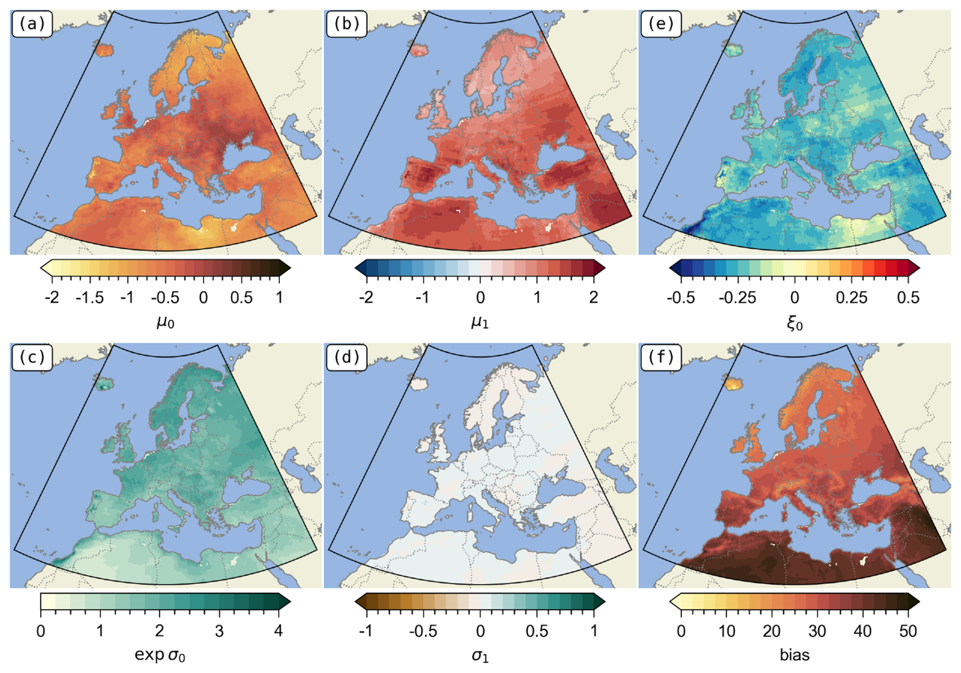
Figure 5 Map of the different parameters of the GEV model after observational constraints. (a) Constant of the location parameter μ₀. (b) Trend of the location parameter μ₁. (c) Constant of the scale parameter exp (σ₀). (d) Trend of the scale parameter σ₁. (e) Constant of the shape parameter ξ₀. (f) Bias of TX3x from ERA5 (mean over 1961/1990).

We start by looking at the current state of return times and intensity change, defined as $\mathrm{\Delta }{I}_t:=I_t^{\mathrm{F}}-I_t^{\mathrm{C}}$ (from Eq. 8), see Sect. 5.1. We then continue with the near future in 2040, see Sect. 5.2. We finish with the end of the 21st century, see Sect. 5.3.

5.1 Current situation: 2024

Figure 6 shows the estimated return times of the maximum observed in between 2024 and 1940 in the counterfactual and factual world (Fig. 6a–b), as well as the change in intensity (Fig. 6c). The 95 % confidence intervals are given in Figs. S6 and S7. It should be noted that in 2024 we are in the projection period (2015 to 2100), and therefore we potentially have several choices. At this point, we consider the influence of the choice of scenario to be too weak (compared to the internal variability), and we have therefore represented the average of the four scenarios.

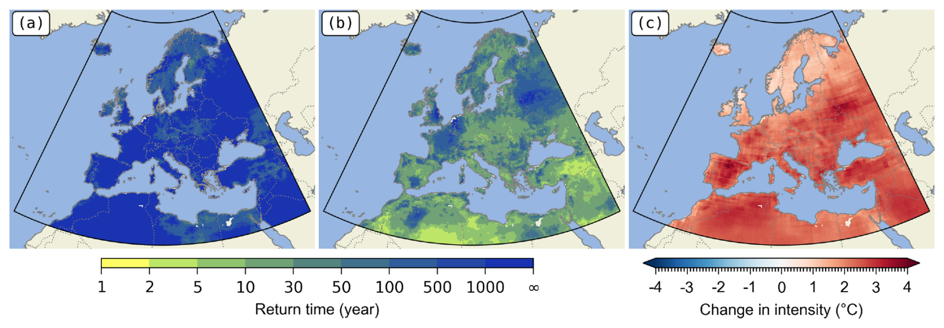
Figure 6 (a) Return time of the maximum observed between 1940 and 2024 in TX3x over Europe, in 2024, without human influence. (b) Same as (a), but for the factual world. (c) Change in intensity in 2024. Lower and upper confidence intervals (95 %) are given in Figs. S6 and S7.

We can see that the counterfactual world shows return times (Fig. 6a) greater than 1000 years over almost the whole of Europe, showing that the maxima currently recorded are almost impossible without anthropogenic climate change. The 95 % confidence interval shows values down to 30 years over North Africa, Central Europe and Northern Europe, but almost the entire domain shows return periods of the order of at least 500 years.

In the factual world, North Africa shows return periods of 2 to 5 years (Fig. 6b), whereas in the counter-factual world they were in excess of 1000 years, showing that near-impossible events are currently becoming the new standard in this part of Europe. The same phenomenon can be seen over Western and Southern Asia, with equivalent values. The 95 % confidence intervals show the same phenomenon.

The temperature increase from the counter-factual to the factual world (Fig. 6c) is fairly uniform across the domain, with values around +2 K. The change is nevertheless marked in Northern Europe, with values of around +1.5 K. The signal remains clearly positive, with the low value of the confidence interval around +1.5 K, and falling to +0.6 K in Northern Europe. The high end of the confidence interval is closer to +3 K, with peaks at +3.7 K.

In line with all the studies on the attribution of extreme temperatures, it is clear that anthropogenic climate change implies a sharp increase in extreme temperatures. The sign of this change is unambiguous, as the low value of the confidence interval does not include a zero or negative change.

Let us finish with spatial variability, which appears to show breaks. Indeed, we can see that in Algeria, the return periods in Fig. 6b can vary very rapidly from a value greater than 1000 years to less than 30 years. To understand this phenomenon, we have shown three series extracted from ERA5 in Fig. S8: one in Paris and two in Algeria showing very different return periods. On these series (the black dots), we superimposed return periods of 2, 5, 10, 30, 50, 100, and 1000 years. In order to verify the quality of the fit for our three series, we have also displayed a histogram of the p-values of the Kolomogorov-Smirnov (KS) tests between 1000 draws of the GEV and ERA5 parameters. We can see that in at least 89 % of cases, the KS test gives a p-value greater than 5 %, showing that we cannot reject the hypothesis that the data are indeed derived from the inferred distribution. This therefore validates our fit. The difference between the series with a return period of >1000 years and the series with a return period of <30 years is the existence of an extreme event which does not change the adjustment but alters the value of the maximum observed. The spatial variability can therefore be explained by the existence or absence of an intense heatwave.

5.2 Mid-term: 2040

First and third rows of the Fig. 7 show the return times in 2040 in the counterfactual and factual world (Fig. 7a–e), as well as the change in intensity (Fig. 7k–n). The 95 % confidence intervals are given in Figs. S9a–e, k–n and S10a–e, k–n. Table S2 gives a summary of the statistics by scenario and country. The 95 % confidence interval is given in Tables S3 and S4.

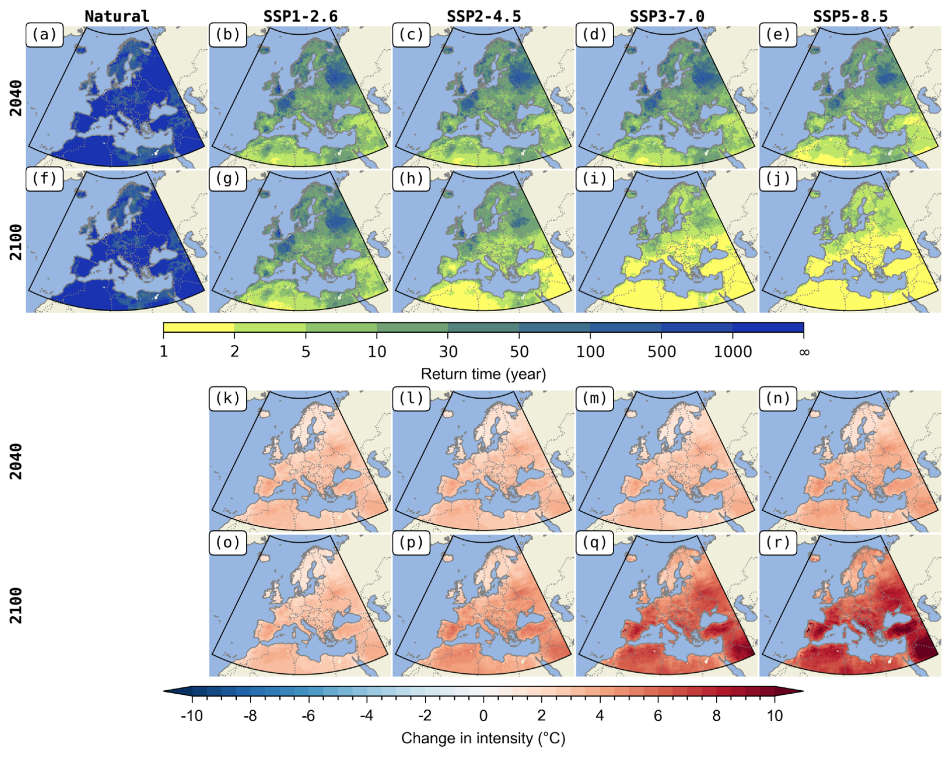
Figure 7 Projection of return time (1st and 2nd row) and change in intensity (3rd and 4th row) in 2040 (1st and 3rd row) and 2100 (2nd and 4th row) of the attribution of the maximum event observed in TX3x between 1940 and 2024. In columns: in the counter-factual world and for the four scenarios SSP1-2.6, SSP2-4.5, SSP3-7.0 and SSP5-8.5. Lower and upper confidence intervals (95 %) are given in Figs. S9 and S10.

For return times, the counterfactual world (Fig. 7a) is the same as that in 2024 (Fig. 6a), and shows return times of over 1000 years. The SSP2-4.5, SSP3-7.0 and SSP5-8.5 scenarios (Fig. 7c–e) are extremely close to each other, with values between 10 and 30 years over most of Europe, falling to 1 to 2 years over North Africa. Overall, the events are more likely than at present, reflecting the rise in temperatures over 16 years. However, these 3 scenarios have not yet been differentiated, unlike SSP1-2.6, which shows slightly longer return periods. Northern France, Belgium, Great Britain and Russia also show slightly longer return periods, between 50 and 500 years. The 95 % confidence interval (Figs. S9a–e and S10a–e) shows a similar message: the three scenarios SSP2-4.5, SSP3-7.0 and SSP5-8.5 are extremely close, and SSP1-2.6 has slightly longer return times.

The change in intensity in 2040, visible in Fig. 7k–n, shows, similarly to the return times, very close values – around +3 to +3 K – for the three scenarios SSP2-4.5, SSP3-7.0 and SSP5-8.5, and a scenario SSP1-2.6 with lower intensity changes of around 0.5 K. Northern Europe shows lower values, below +2 K, while Eastern and Southern Europe reach almost +4 K. The 95 % confidence intervals (Figs. S9k–n and S10k–n) show a similar spatial dispersion of values, with 1 K lower values for the lower bound, and 1 K higher values for the upper bound. Some countries even show changes of more than +5 K.

5.3 Long-term: 2100

Figure 7f shows the return times in 2100 of the maximums observed in the counterfactual world, as the values are the same as for Fig. 7a, the conclusions of Sect. 5.2 apply.

Let us continue with the scenarios, represented on the Fig. 7g–j. Return times decrease with simulated climate change intensity. For SSP1-2.6, only 12 countries (on 55) show return times beyond 50 years, with 28 countries already having a return time of 10 years or less. From SSP2-4.5 onwards, the current maximums are almost commonplace, with only one country showing a return period in excess of 50 years. From SSP3-7.0 onwards, current maximums are the “normal” situation, with return times between 1 to 10 years and 1 to 2 years. The 95 % confidence interval is shown in Figs. S9g–d and S10g–d, and shows that return periods can fall below 10 years over the whole of Europe.

The scenarios for intensity change are represented on the Fig. 7o–r. For scenario SSP1-2.6, the change ranges from +1.7 K for Northern Europe to +4.1 K for Southern Europe, with the change relative to 2024 being almost the same everywhere, around +1 K. For the SSP2-4.5 scenario, the change ranges from +2.7 K for Northern Europe to +6.5 K for Southern Europe. The different regions of Europe show different changes compared to today, ranging from +1.5 to +3.8 K. The SSP3-7.0 and SSP5-8.5 scenarios show increasing intensity increases, from +5 to +9 K. The 95 % confidence interval (Figs. S9o–r and S10o–r) even shows changes in intensity of up to +18 K.

6 Conclusions and perspectives

6.1 Conclusions

In this paper, we have presented an extension of the Robin and Ribes (2020a) method for estimating probabilities of extremes following a GEV law. Our new method allows us, on the one hand, to treat several scenarios simultaneously, and on the other, to force a counter-factual world that is common to all scenarios. We first applied this method to temperature extremes over Paris (France), and demonstrated not only its validity, but also that it drastically reduces differences in the counter-factual probabilities, reinforcing the inter-scenario consistency of our estimates. We have also verified that our estimates of current and future global climate change are consistent with current literature.

We also offer an open-source software that can be used to reproduce our results and easily applied to other fields. This tool is natively parallelized, with particular attention paid to the memory used. It can be deployed just as easily on a personal computer, a computing cluster or a supercomputer. This software is also extensible, and other probability distributions – such as the Normal or Generalized Pareto Distribution – may be integrated in the future.

We have applied this new approach and tool to the attribution of observed maxima over Europe, enabling us to analyze these statistics up to the end of the 21st century for four climate scenarios. In the future, the observed maxima will become the new norm for scenarios greater than the SSP2-4.5 and SSP3-7.0, and will be 2 to 3 K warmer even for a low-emission scenario like the SSP1-2.6. An increase in extreme temperatures of more than 10 K is conceivable within the 95 % confidence interval. We have focused on Europe here, but an extension to the rest of the world and to temperature-like variables such as the heat-index would enable a global map of future heat hazards to be drawn up.

Compared to other studies (such as Vautard et al., 2020; Brown et al., 2014), the estimated return times and intensity changes can be different. This is due to different choices in the statistical model (regional covariate, smoothing method, counterfactual construction), as well as in the estimation method. As shown with the example of Paris, the use of direct observations gives a much stronger (and much more uncertain) trend, while the use of climate simulations as a prior allows for a stronger constraint on the signal. From this perspective, our approach appears much more robust. We should also note the strong influence of the choice of observation data (or similar), given the significant biases on extremes between E-OBS and ERA5. Even though datasets like ERA5 are available on a global scale, the calculation of return times (especially for impact studies) should probably be done from datasets closer to observations (such as E-OBS or stations). Several additional studies are needed to validate or refine the choices made, particularly with regard to the statistical model and the smoothing method.

6.2 Perspectives

Even improvements to the GEV model are possible. For example, the GEV model tends to overestimate return times (see, e.g. Diffenbaugh, 2020; Zeder et al., 2023; Jewson et al., 2025). Recent work by Noyelle et al. (2026) proposed a new GEV model where the upper bound on temperatures is imposed by physics (Zhang and Boos, 2023; Noyelle et al., 2023). This approach would fit in naturally with the tools developed here. A similar method could be applied to precipitation by mixing an estimation of the upper bound (Martin et al., 2025) with a statistical model as the extended Generalized Pareto Distribution (Naveau et al., 2016). Another interesting possibility would be to use external forcings directly as covariates rather than their responses (global and regional temperatures).

Further work is also needed to extend our model to other variables such as wind and precipitation. The tools and statistical model developed here were developed in the context of attribution, particularly in relation to heat waves. Several studies use other types of covariates (such as CO₂ or Z₅₀₀, see, e.g.,  Smith et al., 2021; Auld et al., 2023) or statistical models. Extending this to other variables would require work similar to that of Robin and Ribes (2020a), where the validity of the statistical model was verified in each climate model, as well as its quality after applying observational constraints.

It should also be noted that, on the one hand, we have remained in a univariate context, while the estimation of concurrent events increasing impacts appears increasingly necessary; and on the other hand, spatial structures are ignored. We also used only GCMs, which do not capture local specificities. The use of regional models (when those from CMIP6 become available) will allow us to refine the results obtained here (work in this direction has already been carried out by  Brown et al., 2014), and ANKIALE will make this easy to do.

Finally, the analyses produced here provide local information on the worst possible future events, and show the need for rapid adaptation to extremes warming faster than global warming.

Appendix A: Generalized Extreme Value distribution

The maxima of a variable can be modelled using the GEV distribution (Generalised Extreme Value, see the book by Coles, 2001). This distribution has three parameters:

• The location parameter μ, similar to the mean;

• The scale parameter σ, similar to the standard deviation;

• The shape parameter ξ which controls the type of extreme. If ξ<0, the extremes are bounded, if ξ>0 the distribution is said to be heavy-tailed.

Noting $x_{+}:=max(\mathrm{0},x)$, the cumulative distribution function F_GEV (and the survival function 1−F_GEV) of a random variable $T\sim \mathrm{GEV}(\mathit{\mu },\mathit{\sigma },\mathit{\xi })$ is given by an analytical equation (when $\mathrm{1}+\mathit{\xi }\frac{x-\mathit{\mu }}{\mathit{\sigma }}\ge \mathrm{0})$:

$$\begin{array}{rl}{F}_{\mathrm{GEV}}(x;\mathit{\mu },\mathit{\sigma },\mathit{\xi })& :=\mathbb{P}(T<x)\\ & =\exp \left[-{\left(\mathrm{1}+\mathit{\xi }{\displaystyle \frac{x-\mathit{\mu }}{\mathit{\sigma }}}\right)}_{+}^{-\mathrm{1}/\mathit{\xi }}\right].\end{array}$$

The quantile function 𝒬_GEV (inverse of the distribution function) is also given by:

$${\mathcal{Q}}_{\mathrm{GEV}}(p;\mathit{\mu },\mathit{\sigma },\mathit{\xi }):=\mathit{\mu }+{\displaystyle \frac{\mathit{\sigma }}{\mathit{\xi }}}\left[(-\log p{)}^{-\mathit{\xi }}-\mathrm{1}\right]=F_{\mathrm{GEV}}^{-\mathrm{1}}\left(p\right).$$

Note that if ξ>0, the distribution is not bounded and is said heavy tail. If ξ<0, the extremes are bounded, with the upper bound B given by:

$$B:=\mathit{\mu }-{\displaystyle \frac{\mathit{\sigma }}{\mathit{\xi }}}.$$

In general, to use the GEV distribution, we use the block-maxima theorem, which states that if we divide a data set into blocks and take the maximum of each block, then asymptotically this random variable follows a GEV distribution. Here, annual maximums are used, and this works well overall with temperature.

Appendix B: Some details about the inference of θ

B1 Fit in the climate models

Our approach therefore begins by inferring the θ_m of the statistical model in Eq. (5) using data from N_M climate models.

For each climate model m, we have three time series (with possible repetitions of the time steps for each member) for each SSP scenario:

• ${\stackrel{\mathrm{̃}}{X}}_{t,m}^{\mathrm{R},\mathrm{SSP}}$, regional average temperature series, here for Europe;

• ${\stackrel{\mathrm{̃}}{X}}_{t,m}^{\mathrm{G},\mathrm{SSP}}$, global average temperature series,

• ${\stackrel{\mathrm{̃}}{T}}_{t,m}^{\mathrm{SSP}}$, series of annual maximum temperatures over 3 d.

The inference begins by estimating the parameters of the covariates. Starting from the series ${\stackrel{\mathrm{̃}}{X}}_{t,m}^{\mathrm{R},\mathrm{SSP}}$ and ${\stackrel{\mathrm{̃}}{X}}_{t,m}^{\mathrm{G},\mathrm{SSP}}$, the pair $({\widehat{\mathit{\theta }}}_m^{\mathrm{R}},{\widehat{\mathit{\theta }}}_m^{\mathrm{G}})$ is estimated using the approaches described in Sect. S1.1, as well as the covariance matrix ${\mathbf{\Sigma }}_{({\mathit{\theta }}_m^{\mathrm{R}},{\mathit{\theta }}_m^{\mathrm{G}})}$ describing the uncertainty in this estimation.

Next, we estimate ${\widehat{\mathit{\theta }}}_m^{\mathrm{GEV}}$ from the series ${\stackrel{\mathrm{̃}}{T}}_{t,m}^{\mathrm{SSP}}$ of each model. To do this, we use the vector $({\widehat{\mathit{\theta }}}_m^{\mathrm{R}},{\widehat{\mathit{\theta }}}_m^{\mathrm{G}})$ to generate the forcings $X_{t,m}^{\mathrm{R},\mathrm{SSP}}$. The vector ${\widehat{\mathit{\theta }}}_m^{\mathrm{GEV}}$ can thus be calculated by maximum likelihood, which allows us to estimate ${\widehat{\mathit{\theta }}}_m=({\widehat{\mathit{\theta }}}_m^{\mathrm{R}},{\widehat{\mathit{\theta }}}_m^{\mathrm{G}},{\widehat{\mathit{\theta }}}_m^{\mathrm{GEV}})$. The covariance matrix ${\mathbf{\Sigma }}_{{\widehat{\mathit{\theta }}}_m}={\mathbf{\Sigma }}_{({\mathit{\theta }}_m^{\mathrm{R}},{\mathit{\theta }}_m^{\mathrm{G}},{\mathit{\theta }}_m^{\mathrm{GEV}})}$ of ${\widehat{\mathit{\theta }}}_m$ is estimated using a bootstrap on the series ${\stackrel{\mathrm{̃}}{T}}_{t,m}^{\mathrm{SSP}}$ and the forcings $X_{t,m}^{\mathrm{R},\mathrm{SSP}}$, forcings constructed from several samples according to the normal distribution $\mathcal{N}\left(\right({\widehat{\mathit{\theta }}}_m^{\mathrm{R}},{\widehat{\mathit{\theta }}}_m^{\mathrm{G}}),{\mathbf{\Sigma }}_{({\mathit{\theta }}_m^{\mathrm{R}},{\mathit{\theta }}_m^{\mathrm{G}})})$.

Note that this approach is purely frequentist, in the sense that we estimate the value of θ_m and its covariance matrix, as opposed to the Bayesian view, where we want to determine the distribution of θ_m.

B2 Construction of the prior

The prior is then constructed as a synthesis of climate models. This is where we switch to a Bayesian view: θ is no longer seen as a value to be estimated but as a random vector. For each climate model, we then define the random variable θ_m, which follows the following multivariate normal distribution:

$${\mathit{\theta }}_m\sim \mathcal{N}\left({\widehat{\mathit{\theta }}}_m,{\mathbf{\Sigma }}_{{\widehat{\mathit{\theta }}}_m}\right)$$

Following the work of Ribes et al. (2017), we assume that reality is statistically indistinguishable from a set of climate models (see also Annan and Hargreaves, 2010; Rougier et al., 2013). This allows us to construct a multi-model synthesis ${\mathit{\theta }}_{\ast }\sim \mathcal{N}\left({\widehat{\mathit{\theta }}}_{\ast },{\mathbf{\Sigma }}_{{\widehat{\mathit{\theta }}}_{\ast }}\right)$ which also follows a normal distribution with parameters:

$$\left\{\begin{array}{ll}{\widehat{\mathit{\theta }}}_{\ast }& =\frac{\mathrm{1}}{N_M}\sum _m{\widehat{\mathit{\theta }}}_m,\\ {\mathbf{\Sigma }}_{{\widehat{\mathit{\theta }}}_{\ast }}& =\left(\mathrm{1}+\frac{\mathrm{1}}{N_M}\right){\widehat{\mathbf{\Sigma }}}_u+\mathrm{1}/N_M^{\mathrm{2}}\sum _m{\mathbf{\Sigma }}_{{\widehat{\mathit{\theta }}}_m}.\end{array}\right.$$

In this last equation, the matrix ${\widehat{\mathbf{\Sigma }}}_u$ describes the internal variability of the models. The mathematics describing this approach can be found in Sect. S1.2.

B3 Derivation of the posterior

For the construction of the posterior, we have the observations $X_t^{\mathrm{o},\mathrm{R}}$, $X_t^{\mathrm{o},\mathrm{G}}$ and $T_t^{\mathrm{o}}$ (regional average temperature, global average temperature and temperature extremes). Let us start again from the calculation in Robin and Ribes (2020a, Sect. 3.5), which allows us to separate the conditioning by $X_t^{\mathrm{o},\mathrm{R}}$ and $X_t^{\mathrm{o},\mathrm{G}}$ from that by $T_t^{\mathrm{o}}$. We then have:

$$\begin{array}{}\text{(B1)}& \begin{array}{rl}& \mathbb{P}\left[{\mathit{\theta }}_{\ast }\left|\right(X_t^{\mathrm{o},\mathrm{R}},X_t^{\mathrm{o},\mathrm{G}},T_t^{\mathrm{o}})\right]=\\ & {\displaystyle \frac{\mathbb{P}\left[T_t^{\mathrm{o}}\left|\right({\mathit{\theta }}_{\ast }\left|\right(X_t^{\mathrm{o},\mathrm{R}},X_t^{\mathrm{o},\mathrm{G}}\left)\right)\right]\mathbb{P}\left[{\mathit{\theta }}_{\ast }\left|\right(X_t^{\mathrm{o},\mathrm{R}},X_t^{\mathrm{o},\mathrm{G}})\right]}{\mathbb{P}\left(T_t^{\mathrm{o}}\right)}}\end{array}\end{array}$$

The important point is that, starting from the prior θ_∗, we can construct the posterior $\left({\mathit{\theta }}_{\ast }\right|(X_t^{\mathrm{o},\mathrm{R}},X_t^{\mathrm{o},\mathrm{G}}))$, thus defining a new random variable. This latter variable can itself be considered as a prior to be constrained by $T_t^{\mathrm{o}}$, which allows us to derive the complete posterior. This constraint is therefore applied in two steps.

B3.1 Covariables constraint

The estimate of $\left({\mathit{\theta }}_{\ast }\right|(X_t^{\mathrm{o},\mathrm{R}},X_t^{\mathrm{o},\mathrm{G}}))$ is in fact analytical, and the Gaussian conditioning theorem (Eaton, 2007) applies. Let X^o be a global vector of observations that concatenates $X_t^{\mathrm{o},\mathrm{R}}$ and $X_t^{\mathrm{o},\mathrm{G}}$ over time, and ${\mathit{\epsilon }}^{\mathrm{o}}\sim \mathcal{N}(\mathrm{0},{\mathbf{\Sigma }}^{\mathrm{o}})$ be white noise of the same dimension as X^o. If we find a matrix A such that $X^{\mathrm{o}}=\mathbf{A}\cdot {\mathit{\theta }}_{\ast }+{\mathit{\epsilon }}^{\mathrm{o}}$, and since θ_∗ follows a normal distribution, then $\left({\mathit{\theta }}_{\ast }\right|X^{\mathrm{o}})=({\mathit{\theta }}_{\ast }\left|\right(X_t^{\mathrm{o},\mathrm{R}},X_t^{\mathrm{o},\mathrm{G}}\left)\right)$ also follows a normal distribution, i.e. $\left({\mathit{\theta }}_{\ast }\right|X^{\mathrm{o}})\sim \mathcal{N}({\mathit{\mu }}_{\left({\mathit{\theta }}_{\ast }\right|X^{\mathrm{o}})},{\mathbf{\Sigma }}_{\left({\mathit{\theta }}_{\ast }\right|X^{\mathrm{o}})})$, with value:

$$\left\{\begin{array}{ll}{\mathit{\mu }}_{\left({\mathit{\theta }}_{\ast }\right|X^{\mathrm{o}})}& ={\mathit{\theta }}_{\ast }+\left({\mathbf{\Sigma }}_{{\mathit{\theta }}_{\ast }}{\mathbf{A}}^T\right)\cdot (\mathbf{A}{\mathbf{\Sigma }}_{{\mathit{\theta }}_{\ast }}{\mathbf{A}}^T+{\mathbf{\Sigma }}^{\mathrm{o}}{)}^{-\mathrm{1}}\\ & \cdot (X^{\mathrm{o}}-\mathbf{A}{\mathit{\theta }}_{\ast }),\\ {\mathbf{\Sigma }}_{\left({\mathit{\theta }}_{\ast }\right|X^{\mathrm{o}})}& ={\mathbf{\Sigma }}_{{\mathit{\theta }}_{\ast }}-\left({\mathbf{\Sigma }}_{{\mathit{\theta }}_{\ast }}{\mathbf{A}}^T\right)\cdot (\mathbf{A}{\mathbf{\Sigma }}_{{\mathit{\theta }}_{\ast }}{\mathbf{A}}^T+{\mathbf{\Sigma }}^{\mathrm{o}}{)}^{-\mathrm{1}}\\ & \cdot \left(\mathbf{A}{\mathbf{\Sigma }}_{{\mathit{\theta }}_{\ast }}\right).\end{array}\right.$$

The difficulties here are constructing the matrix A, which models how our parameters are transformed into the observation signal, and estimating Σ^o, which models the internal variability of the observations.

For matrix A, two approaches are proposed in Sect. S1.3.1. One is based on the idea that, over the observed period, the scenarios are sufficiently similar that their mean can be projected onto the observations. The second requires choosing a scenario. In this article, we will use the first approach.

For the covariance matrix Σ^o, two approaches are also proposed in Sect. S1.3.2. The first is simply to consider it as white noise, estimates of observations from which a trend has been removed. The second approach was developed by Ribes et al. (2021) and Qasmi and Ribes (2022), and assumes that ε^o takes the form of a sum of two first-order autoregressive processes. One is fast to model inter-annual variability, while the second is slow to model decadal variability. In this article, we will use the first approach.

B3.2 Variable constraint

With our knowledge of the distribution $\left({\mathit{\theta }}_{\ast }\right|(X_t^{\mathrm{o},\mathrm{R}},X_t^{\mathrm{o},\mathrm{G}}))$, we now want to obtain samples of the distribution $\left(\right[{\mathit{\theta }}_{\ast }\left|\right(X_t^{\mathrm{o},\mathrm{R}},X_t^{\mathrm{o},\mathrm{G}}\left)\right]\left|T_t^{\mathrm{o}}\right)$. The whole problem is that $T_t^{\mathrm{o}}$ follows a GEV distribution, and there is no explicit expression for the posterior. Let us start again from the Eq. (B1).

• The term $\mathbb{P}\left[{\mathit{\theta }}_{\ast }\right|(X_t^{\mathrm{o},\mathrm{R}},X_t^{\mathrm{o},\mathrm{G}})]$ is known, it is our prior.

• The term $\mathbb{P}\left[T_t^{\mathrm{o}}\right|\left({\mathit{\theta }}_{\ast }\right|(X_t^{\mathrm{o},\mathrm{R}},X_t^{\mathrm{o},\mathrm{G}})\left)\right]$ is directly calculable: the draws generate the parameters of the GEV law, which can thus be evaluated.

• When the denominator is analytically intractable, numerical methods are necessary to sample from the posterior distribution.

A common approach to perform this sampling is the Metropolis-Hasting algorithm (Metropolis et al., 1953), (Hastings, 1970). This is the sampling algorithm originally used by Robin and Ribes (2020a). This Markov chain Monte Carlo algorithm relies on a random walk proposal: a new proposal is created by starting from an initial value θ₀ and adding a random noise to generate a θ₁. The new value is either accepted or rejected with a probability defined using the likelihood ratio of the proposal and the previous value. A key element of this procedure is the transition function between θ_i and θ_i+1 that is used to sample successive possible values of the posterior.

In the Robin and Ribes (2020a) original implementation, the transition function was of the form ${\mathit{\theta }}_{i+\mathrm{1}}={\mathit{\theta }}_i+\mathit{\epsilon }$ where ε follows a normal distribution with the same scale for all parameters. This can become an issue when the scale of the target parameters is very different from one another. The transition also determines the rate of convergence and mixing, so this implementation can be computationally sub-optimal. Various diagnostics showed the algorithm suffered from slow-mixing chains (Gelman et al., 1997), high autocorrelation (Brooks et al., 2011), and low effective sample size (Gelman et al., 2015).

To deal with these issues, we leverage the No-U-Turn Sampler algorithm NUTS, (Hoffman and Gelman, 2014), as implemented in STAN (Stan Development Team, 2024). This algorithm is based on the Hamiltonian Monte Carlo algorithm (Radford, 2011), a variant of the Metropolis-Hasting algorithm where the proposal is not generated using a random walk. Instead, the proposal is created through a series of gradient-informed steps (Betancourt, 2018). This allows for better parameter space exploration, especially in the multidimensional case. The NUTS variant relies on a specific criteria to select adaptively various hyper-parameters such as the steps length and stopping conditions. This adaptation makes the algorithm more robust against correlation in the posterior. The NUTS algorithm is particularly effective when the posterior dimensions are correlated or of different scales. It is very efficient to explore the parameter space and draw samples from the posterior.