Selecting a conceptual hydrological model using Bayes' factors computed with replica-exchange Hamiltonian Monte Carlo and thermodynamic integration

We develop a method for computing Bayes' factors of conceptual rainfall–runoff models based on thermodynamic integration, gradient-based replica-exchange Markov chain Monte Carlo algorithms and modern differentiable programming languages. We apply our approach to the problem of choosing from a set of conceptual bucket-type models with increasing dynamical complexity calibrated against both synthetically generated and real runoff data from Magela Creek, Australia. We show that using the proposed methodology, the Bayes factor can be used to select a parsimonious model and can be computed robustly in a few hours on modern computing hardware.

1 Introduction

Hydrologists are often faced with assessing the performance of models that differ in their complexity and ability to reproduce observed data. The Bayes factor (BF) is one method for selecting between models from an a priori chosen set (Berger and Pericchi, 1996). The appeal of the BF lies in its ability to implicitly and automatically balance model complexity and goodness of fit with few simplifying assumptions. The BF is also invariant to data and parameter transformations unlike information-theory-based criteria, such as Akaike information criterion (AIC) and the Bayesian information criterion (BIC) (O'Hagan, 1997). For example, a logarithmic transformation of the discharge or the square root of a parameter such as the flow rate can accelerate the convergence of the model, but it will not affect the computed BF.

However, the BF requires the computation of the marginal likelihood (the denominator in Bayes' theorem) for each model, which is a difficult and expensive integration problem. This expense and difficulty can be attributed to three main factors; the necessity of many model runs at different points in the parametric space; the possibly multimodal and highly correlated nature of the posterior that can lead to isolated and/or slowly mixing chains; and, finally, the inherent difficulty of the marginal likelihood integration problem.

Because of these difficulties, it is the case today that the BF is not widely used by practitioners despite it being a crucial component in Bayesian model comparison, selection, and averaging (Höge et al., 2019). This stands in contrast with the widely studied and used Bayesian parameter estimation procedure (Gelman et al., 2020). Consequently, model uncertainty is often ignored or assessed by either ad hoc techniques or information-theoretic criteria (Birgé and Massart, 2007; Bai et al., 1999) that explicitly (rather than implicitly) penalize model complexity based on some measure of the number of parameters and under limiting assumptions; see, for example, Berger et al. (2001) for a full discussion.

1.1 Background

Looking outside of hydrology, there are a number of notable works that have developed techniques for numerically estimating the BF. A recent comprehensive review by Llorente et al. (2023) discusses the relative advantages of commonly used methods for computing the marginal likelihood and consequently, the BF, such as the naive Monte Carlo methods, harmonic mean estimator (Newton and Raftery, 1994); generalized harmonic mean estimator (Gelfand and Dey, 1994); importance sampling and Chib's method (Chib and Jeliazkov, 2001; Chib, 1995); bridge sampling (Meng and Wong, 1996; Gelman and Meng, 1998); nested sampling (Skilling, 2004, 2006); and, finally, thermodynamic integration (Calderhead and Girolami, 2009; Lartillot and Philippe, 2006; Ogata, 1989), the technique that we choose to use in this study. Thermodynamic integration is well suited for high-dimensional integrals (Ogata, 1989, 1990) involving physics-based models, such as ordinary differential equation (ODE) systems. The naive Monte Carlo is unstable and usually not efficient, requiring a huge number of samples for convergence. Importance sampling and harmonic estimators require a suitable choice of the importance and proposal distributions, respectively. The performance of bridge sampling also depends on a good choice of proposal distribution, which in practice is not straightforward to determine a priori. The main difficulty with nested sampling is generating samples from a truncated prior as the threshold increases (Chopin and Robert, 2010; Henderson and Goggans, 2019). However, the efficiency of Chib's method depends on how close an arbitrary value is to the posterior mode (Dai and Liu, 2022). Hug et al. (2016) illustrated that Chib's method significantly underestimates the marginal likelihood of a bimodal Gaussian mixture model.

Turning our attention to works within hydrology that develop methods for computing Bayes' factors, to the best of our knowledge, the seminal work by Marshall et al. (2005) was the first to propose computing Bayes' factors for hydrological model selection. Marshall et al. (2005) used Chib's method to estimate the marginal likelihood of conceptual models. More recently, various other authors  (Liu et al., 2016; Brunetti et al., 2019, 2017; Volpi et al., 2017; Cao et al., 2019; Brunetti and Linde, 2018; Marshall et al., 2005) have considered the computation of Bayes' factors in a hydrological or hydrogeological context.

Perhaps most closely related to our study are the recent works of Brunetti et al. (2019, 2017) and Brunetti and Linde (2018), who computed Bayes' factors for conceptual hydrogeological models with thermodynamic integration techniques. Brunetti et al. (2017) compared naive Monte Carlo, bridge sampling based on the proposal distribution developed by Volpi et al. (2017), and the Laplace–Metropolis method in terms of calculating the marginal likelihood of conceptual models. Like most studies, the naive Monte Carlo approach performed poorly. Also, Brunetti and Linde (2018) computed the marginal likelihood using methods based on a proposal distribution, notably bridge sampling. Several marginal likelihood estimation methods have been compared within hydrological studies. For example, Liu et al. (2016) found that thermodynamic integration gives consistent results compared to nested sampling and is less biased.

Many studies in hydrology (e.g. Zhang et al., 2020; Brunetti et al., 2017; Zheng and Han, 2016; Shafii et al., 2014; Laloy and Vrugt, 2012, and Kavetski and Clark, 2011) have used the Differential Evolution Adaptive Metropolis (DREAM) algorithm (Vrugt, 2016) for posterior parameter inference. Volpi et al. (2017) introduced a method to construct the proposal distribution for bridge sampling and integrated it into the DREAM algorithm. However, it still requires the user to choose the number of Gaussian distributions for the Gaussian mixture proposal distribution. The DREAM algorithm has been developed with an acceptance rate similar to the random walk Metropolis (RWM) algorithm, which has an optimal acceptance rate of 0.234 (Vrugt et al., 2008; Gelman et al., 1996b; Roberts and Rosenthal, 2009). The acceptance rate or probability is the proportion of the proposed samples accepted in the Metropolis–Hastings algorithm. In contrast, a gradient-based sampler such as Hamiltonian Monte Carlo (HMC), which we use in this work, typically has a far higher optimal acceptance rate of around 0.65 (Radford, 2011; Beskos et al., 2013). In addition, gradient-based samplers show improved chain mixing properties in high dimensions and on posteriors with strongly correlated parameters (Radford, 2011). Gradient-based algorithms have been used in hydrology for parameter estimation but not model selection. For instance, Hanbing Xu and Guo (2023) found that the No-U-Turn Sampler (NUTS) (Hoffman and Gelman, 2014) performed well for calibrating a model of daily runoff predictions of the Yellow River basin in China. Krapu and Borsuk (2022) employed HMC to calibrate the parameters of rainfall–runoff models. The model selection studies by Liu et al. (2016) and Brunetti et al. (2017, 2019) that use the BF use posterior samples from the DREAM algorithm and consequently a lower acceptance rate than gradient-based samples, e.g. HMC. In addition, because gradient-based samplers incorporate information about the local geometry of the posterior, they are usually easier to tune to achieve the optimal acceptance rate, particularly in the moderate- or high-dimensional parameter setting (the number of parameters being >5).

1.2 Contribution

The overall contribution of this paper is to describe the development of a method, replica-exchange preconditioned Hamiltonian Monte Carlo (REpHMC), which, when used in conjunction with thermodynamic integration (TI), can be used to estimate the BF of competing conceptual rainfall–runoff hydrological models. Our approach for estimating the marginal likelihood combines TI for marginal likelihood estimation, replica-exchange Monte Carlo (REMC) for power posterior ensemble simulation, and preconditioned Hamiltonian Monte Carlo (pHMC) for highly efficient gradient-based sampling which together we call the REpHMC + TI estimator. We demonstrate that REpHMC can sample from moderate-dimensional, strongly correlated, and/or multimodal distributions that frequently arise from hydrological models. In addition, REpHMC + TI can obtain posterior parameter estimates and the marginal likelihood simultaneously. We remark that Brunetti et al. (2019) also suggested, but did not explore, the idea of using REMC (therein called parallel tempering Monte Carlo) to improve chain mixing in hydrological models. Two other gradient-based samplers, Metropolis-adjusted Langevin algorithm (MALA) (Xifara et al., 2014) and NUTS (Hoffman and Gelman, 2014) are used briefly in this paper as a point of comparison, but we do not include their detailed derivation.

Another key contribution of our work compared with, for example, Brunetti et al. (2017, 2019) is the incorporation of recent ideas from probabilistic programming for the automatic specification of Bayesian inference problems (parameter and BF estimation). Utilizing recent techniques from the literature on neural ordinary differential equations (ODEs) (Chen et al., 2018; Rackauckas et al., 2020; Kelly et al., 2020), we formulate a set of models like Hydrologiska Byråns Vattenbalansavdelning (HBV) with extensible model complexity as a system of ordinary differential equations (ODEs). Working in this framework allows us to use efficient high-order time-stepping schemes for the numerical solution of the ODE system and to automatically derive the associated continuous adjoint ODE system. With this adjoint system, we can efficiently calculate the derivative of the posterior functional with respect to the model parameters, a necessary step for working with gradient-based samplers such as HMC. We emphasize at this point that our approach is largely free of manual tuning parameters and straightforward to implement in a differentiable programming framework (we use TensorFlow probability (TFP) (https://www.tensorflow.org/probability, last access: 22 February 2023) with the JAX (https://www.tensorflow.org/probability/examples/TensorFlow_Probability_on_JAX, https://docs.jax.dev, last access: 25 February 2025) backend, but the ideas are applicable in similar frameworks such as Stan (https://mc-stan.org/, last access: 22 February 2023) or PyMC3 (https://www.pymc.io/projects/docs/en/v3/index.html, last access: 22 February 2023). We remark that a recent, more theory-focused paper (Henderson and Goggans, 2019) also proposed using TI with HMC via the Stan probabilistic programming language, but with results for non-time series models and without using REMC, which is an important aspect of our approach.

After model selection via the BF, it is essential to check if the chosen model can generate the observed data. Hydrographs show the time series of streamflow. However, formal goodness-of-fit testing is necessary since it is challenging to see a mismatch in hydrographs for dense data. We therefore use the prior-calibrated posterior predictive p value (PCPPP), which simultaneously tests for prior data conflict and discrepancies in the model for further improvements.

In summary, this paper is the first to propose the REpHMC + TI method in a probabilistic programming framework for the estimation of marginal likelihoods related to hydrological systems in view of model selection. We demonstrate the performance of our method by showing (a) a validation of the methodology using an analytically tractable model, (b) its improved efficiency with respect to classical methods using artificially generated data, and (c) an application of a Bayes-factor-based model selection on real rainfall/runoff data collected from the Magela Creek catchment in Australia.

Our overall perspective is that these techniques have the potential to bring robust model comparison techniques based on BF closer to everyday hydrological modelling practice. Aside from the algorithmic developments in this paper, a necessary technological requirement would be the (re-)implementation of hydrological models in a differentiable programming language, e.g. JAX, PyTorch, or TensorFlow, rather than in a traditional language such as C, Fortran, or Python. While using modern differentiable programming techniques is commonplace for model developers working with machine-learning-type approaches, e.g. neural networks, it is less commonly used, but no less applicable, for more traditional hydrological modelling approaches like the ODE-based HBV-like system we consider here. We hope our results encourage more hydrologists to consider differentiable programming tools for conceptual model implementation given the advantages that derivative-based sampling and optimization algorithms bring to the table in terms of computational efficiency and improved insight, e.g. model selection.

The rest of the paper is organized as follows. Section 2 is about conceptual hydrological models and Bayesian methodology, which includes model formulation, prior and likelihood construction, posterior predictive checks, numerical methods, and algorithms. Section 3 contains the results and discussions, while the conclusions are provided in Sect. 4. There is also a list of acronyms at the end.

2 Methodology

This section describes the model formulation, likelihood construction, algorithms used, and implementation in differentiable software. We leave other modelling aspects, like the type of priors used, for the next section, where we present experiments.

2.1 Conceptual models

We develop a set of rainfall–runoff conceptual hydrological models in the framework of continuous dynamical systems that can be written as a system of ODEs of the following form:

$$\begin{array}{}\text{(1)}& \begin{array}{rl}{\displaystyle }{V}_t& {\displaystyle }=f(t,V,\mathit{\theta })\forall t\in (\mathrm{0},\overline{T}],\\ {\displaystyle }V(t=\mathrm{0})& {\displaystyle }=\widehat{V},\end{array}\end{array}$$

where V are the n system states, $V_t:=\frac{\mathrm{d}V}{\mathrm{d}t}$ is the derivative of the state with respect to the time variable t, $\overline{T}$ is the final time, $\widehat{V}\in {\mathbb{R}}^n$ are the initial conditions, f are known functions, and θ∈ℝ^p is a vector containing the p model parameters.

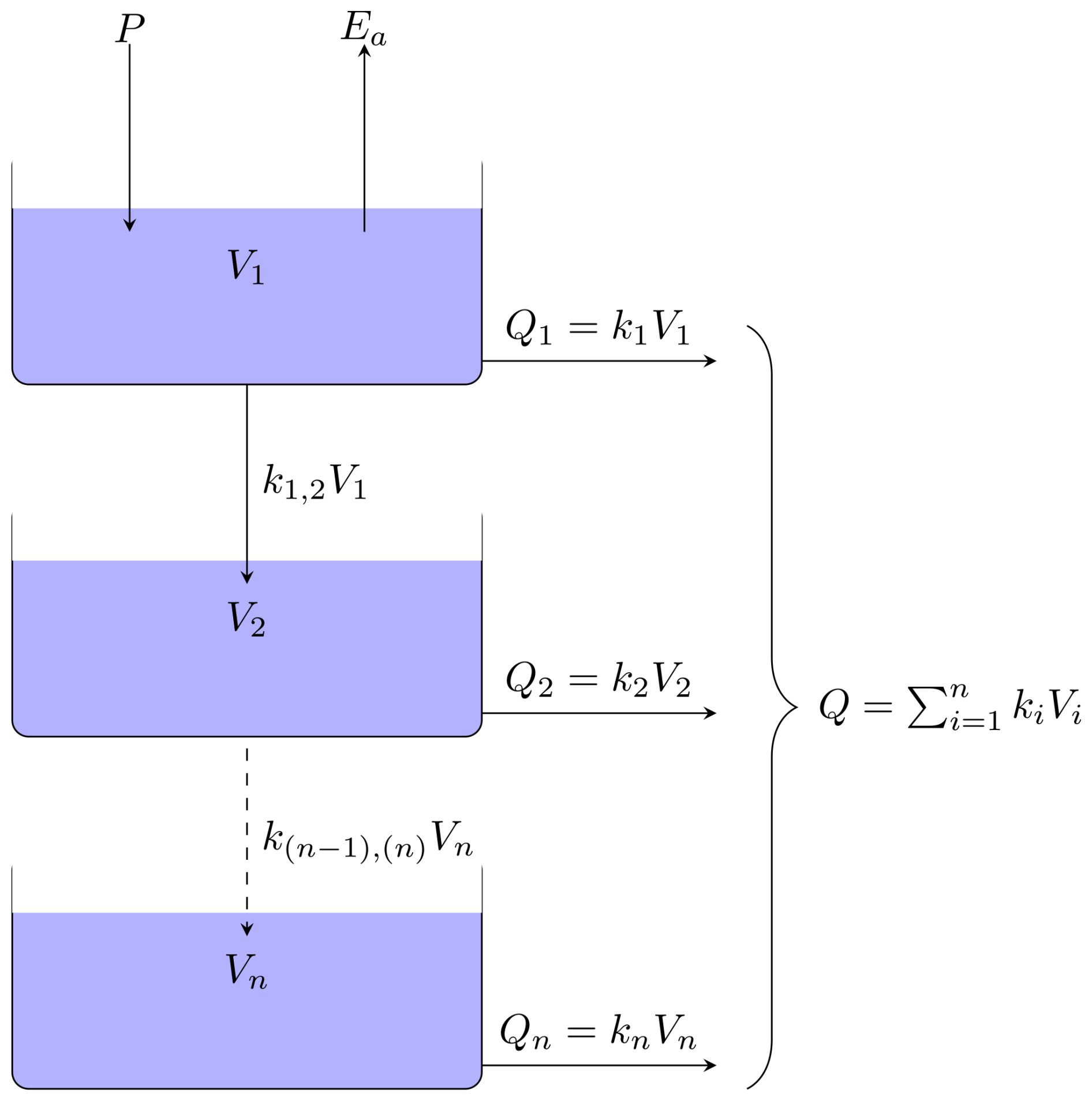
Figure 1 Schematic representation of HBV-like ODE model with n buckets according to the notations in the text. The blue boxes represent the buckets with a given state V₁ to V_n. The solid arrows represent mass flows between buckets into the system or out of the system. The dashed arrow represents the collective mass flow between multiple buckets.

For the purpose of the results in this paper, we derive a set of HBV-like models under the principle of conservation of mass. The algorithms developed in this study can be applied to other bucket-type models, e.g. Parajka et al. (2007), Jansen et al. (2021), or those described in the comprehensive MARRMoT rainfall–runoff models toolbox (Trotter et al., 2022). In comparison with the “standard” HBV model (Bergström, 1976), our model lacks snow and a routing routine, and we choose to replace the traditional soil moisture routine with a linear reservoir. A schematic representation of mass flow between the buckets system is given in Fig. 1. The system states $\mathit{\{}{V}_{\mathrm{1}},\mathrm{\dots },V_n\mathit{\}}$ [L³], where L is a generic length unit, representing the volume of water in the ith bucket, and n is the total number of buckets. The system of ODEs for general n≥1 can be written as follows:

$$\begin{array}{ll}\text{(2a)}& {\displaystyle }(V_{\mathrm{1}}{)}_t& {\displaystyle }=P-E_{\mathrm{a}}-k_{\mathrm{1}}{V}_{\mathrm{1}},n=\mathrm{1},\text{(2b)}& {\displaystyle }(V_{\mathrm{1}}{)}_t& {\displaystyle }=P-E_{\mathrm{a}}-k_{\mathrm{1}}{V}_{\mathrm{1}}-k_{\mathrm{1},\mathrm{2}}{V}_{\mathrm{1}},n\ge \mathrm{2},{\displaystyle }(V_i{)}_t& {\displaystyle }=k_{(i-\mathrm{1}),\left(i\right)}{V}_{i-\mathrm{1}}-k_i{V}_i-k_{\left(i\right),(i+\mathrm{1})}{V}_i,\\ \text{(2c)}& {\displaystyle }& {\displaystyle }i=\mathrm{2},\mathrm{\dots },n-\mathrm{1},n\ge \mathrm{3},\text{(2d)}& {\displaystyle }(V_n{)}_t& {\displaystyle }=k_{(n-\mathrm{1}),\left(n\right)}{V}_{n-\mathrm{1}}-k_n{V}_n,n\ge \mathrm{2},\text{(2e)}& {\displaystyle }V(t=\mathrm{0})& {\displaystyle }=\widehat{V},\text{(2f)}& {\displaystyle }{E}_{\mathrm{a}}& {\displaystyle }={\displaystyle \frac{E_{\mathrm{p}}}{V_{\max }}}{V}_{\mathrm{1}},\text{(2g)}& {\displaystyle }Q& {\displaystyle }=\sum _{i=\mathrm{1}}^n{k}_i{V}_i.\end{array}$$

The parameter $k_{(i-\mathrm{1}),\left(i\right)}$ [T⁻¹], $i=\mathrm{2},\mathrm{\dots },n,$ is the interbucket recession coefficient, where T is a generic time unit. The parameter k_(i) [T⁻¹], $i=\mathrm{1},\mathrm{\dots },n,$ is the outflow recession coefficients. The total outflow, Q [L³ T⁻¹], specified in Eq. (2g) is the noiseless quantity y used in the upcoming calibration and model selection procedures. The precipitation, P [L³ T⁻¹], is an a priori known function of time. Potential evaporation, E_p [L³ T⁻¹], is a known function of time, whereas actual evaporation, E_a [L³ T⁻¹], is a function of E_p, and V_max [L³] through Eq. (2f), where V_max is the maximum amount of water the soil can store. We remark that the term $E_{\mathrm{p}}/V_{\max }$ in Eq. (2f) has the dimension [L³ T⁻¹] and can therefore be thought of as a dynamic recession coefficient with the dynamic behaviour controlled by the known time-varying potential evapotranspiration function, E_p.

The parameter vector θ∈ℝ^p associated with the model is then

$$\begin{array}{}\text{(3)}& \mathit{\theta }:=\mathit{\{}\underset{\mathrm{1}}{\underbrace{V_{\max }}},\underset{n}{\underbrace{k_{\mathrm{1}},\mathrm{\dots },k_n}},\underset{n-\mathrm{1}}{\underbrace{k_{\mathrm{1},\mathrm{2}},\mathrm{\dots },k_{(n-\mathrm{1}),\left(n\right)}}},\underset{n}{\underbrace{{\widehat{V}}_{\mathrm{1}},\mathrm{\dots },{\widehat{V}}_n}}\mathit{\}}.\end{array}$$

The number of buckets can be varied by adjusting $n\in {\mathbb{N}}^{+}$, leading to a set of models, $\mathit{\{}{M}_{\mathrm{1}},\mathrm{\dots },M_n\mathit{\}}$, each with n states and p=3n parameters. Note that for i>j, a more complex model M_i contains a superset of the components of a simpler model M_j. Consequently, after the calibration of both models on a dataset produced by M_j, M_i should be able to reproduce the data as well as M_j but at the cost of higher model complexity. This construction is used in the results to show that the BF does penalize the complex model M_i, leading to the selection of M_j, the expected result.

2.2 Bayesian methodology

We briefly restate the Bayes theorem in order to set our notation. If y is the data and θ the parameter vector associated with a model M, then Bayes' theorem in Eq. (4) defines the posterior probability of θ as

$$\begin{array}{}\text{(4)}& \begin{array}{rl}\underset{\text{posterior}}{\underbrace{\mathit{\pi }\left(\mathit{\theta }\right|y,M)}}& ={\displaystyle \frac{\stackrel{\text{likelihood}}{\overbrace{f\left(y\right|\mathit{\theta },M)}}\stackrel{\text{prior}}{\overbrace{\mathit{\pi }\left(\mathit{\theta }\right|M)}}}{\underset{\text{marginal (averaged) likelihood}}{\underbrace{p\left(y\right|M)}}}}\\ & ={\displaystyle \frac{f\left(y\right|\mathit{\theta },M\left)\mathit{\pi }\right(\mathit{\theta }\left|M\right)}{\int f\left(y\right|\mathit{\theta },M\left)\mathit{\pi }\right(\mathit{\theta }\left|M\right)\mathrm{d}\mathit{\theta }}}.\end{array}\end{array}$$

The prior is a probability distribution of a parameter before data are considered. It can incorporate expert knowledge, historical results, or any belief about the model parameters. The likelihood tells us how likely it is that various parameter values could have generated the observed data. The denominator in Bayes' theorem, that is

$$\begin{array}{}\text{(5)}& p\left(y\right|M)=\int \stackrel{\text{likelihood}}{\overbrace{f\left(y\right|\mathit{\theta },M)}}\stackrel{\text{prior}}{\overbrace{\mathit{\pi }\left(\mathit{\theta }\right|M)}}\mathrm{d}\mathit{\theta },\end{array}$$

is called the marginal likelihood. The marginal likelihood tells us how likely it is that the model supports the data. The distribution of the parameters given the data is known as the posterior and is proportional to the product of the likelihood and the prior. In the Bayesian paradigm, all inference is based on the posterior.

2.2.1 Likelihood construction

In this section, we drop the explicit index on the model for notational convenience. We define a solution operator $G_{\mathrm{sol}}:{\mathbb{R}}^{\mathrm{3}n}\to X$ that maps a parameter vector θ_j to the total outflow function Q. Concretely, this solution operator is calculated by numerically solving Eqs. (2a) to (2g). We then define the observation operator $G_{\mathrm{obs}}:X\to {\mathbb{R}}^q$ which evaluates the solution Q∈X at a set of q points in time $\mathit{\{}{t}_{\mathrm{1}},\mathrm{\dots },t_q\mathit{\}}$.

We assume the following standard Gaussian white noise model for the observed data: $y=G_{\mathrm{obs}}{G}_{\mathrm{sol}}\left(\mathit{\theta }\right)+\mathit{\eta }$, where $\mathit{\eta }\sim \mathrm{MVN}(\mathrm{0},{\mathit{\sigma }}^{\mathrm{2}}{\mathbf{I}}_q)$, with MVN being a multivariate normal distribution with mean 0∈ℝ^q and covariance ${\mathit{\sigma }}^{\mathrm{2}}{\mathbf{I}}_q\in {\mathbb{R}}^{q\times q}$ and σ²∈ℝ the variance of the measurement noise and I_q the usual q-dimensional identity matrix. Let $G:=G_{\mathrm{obs}}{G}_{\mathrm{sol}}:{\mathbb{R}}^{\mathrm{3}n}\to {\mathbb{R}}^q$. By standard arguments it can be shown that $y|\mathit{\theta }\sim \mathrm{MVN}(G\left(\mathit{\theta }\right),{\mathit{\sigma }}^{\mathrm{2}}{\mathbf{I}}_q)$, resulting in the likelihood $f\left(y\right|\mathit{\theta },M)$ in Eq. (4) being fully defined. For brevity, we leave precise prior specifications to the results in Sect. 3.

We remark that according to Cheng et al. (2014), our choice of a likelihood function with Gaussian white noise is equivalent to using the well-known Nash–Sutcliffe efficiency (NSE) as a metric. However, other popular metrics such as Kling–Gupta efficiency (KGE) cannot be explicitly linked with a likelihood function and consequently cannot be used within a formal Bayesian analysis. A recent paper (Liu et al., 2022) proposes an adaptation of the KGE idea using a gamma distribution which can be used as an informal likelihood function within a Bayesian analysis, but we do not explore this option further here. An alternative option which bypasses the need for an explicit likelihood function is approximate Bayesian computation (ABC) could be an appropriate alternative when an appropriate explicit metric or likelihood function is unavailable (see, for example, Nott et al., 2012, and Liu et al., 2023).

2.2.2 Model comparison

The marginal likelihood is also called the normalizing constant (Chen et al., 2000; Gelman and Meng, 1998), prior predictive density, evidence (MacKay, 2003), or integrated likelihood (Lenk and DeSarbo, 2000; Gneiting and Raftery, 2007). This quantity is essential to the definition of the Bayes factor. Indeed, the Bayes factor for two competing models, M_i and M_j, with i≠j, is the ratio of their marginal likelihoods:

$$\begin{array}{}\text{(6)}& {\mathrm{BF}}_{ij}={\displaystyle \frac{p\left(y\right|M_i)}{p\left(y\right|M_j)}}={\displaystyle \frac{\int f\left(y\right|{\mathit{\theta }}_i,M_i\left)\mathit{\pi }\right({\mathit{\theta }}_i\left|M_i\right)\mathrm{d}{\mathit{\theta }}_i}{\int f\left(y\right|{\mathit{\theta }}_j,M_j\left)\mathit{\pi }\right({\mathit{\theta }}_j\left|M_j\right)\mathrm{d}{\mathit{\theta }}_j}}.\end{array}$$

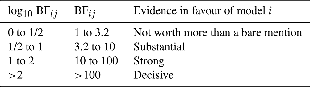
Since BF is a ratio, a value greater than 1 means that M_i should be preferred to M_j and vice versa for a value smaller than 1. Kass and Raftery (1995) proposed a measure of the strength of evidence (Table 1) that we use throughout this paper to interpret the Bayes factors.

An appealing feature of the BF is its consistency in the limit of a high number of observations. Proofs of consistency for non-nested models are in Casella et al. (2009). For other cases, including nonparametric models, a review and detailed study of consistency can be found in Chib and Kuffner (2016). Also, information-theoretic model selection approaches usually require an explicit penalty for the number of model parameters (model complexity). In contrast, the BF implicitly penalizes the complexity of the model. That is, we do not need to assign a penalty for model complexity since it is already accounted for in the marginal likelihood and hence the BF.

Table 1 Interpretation of the Bayes factor (Kass and Raftery, 1995).

2.2.3 Posterior predictive checks

Model selection does not reveal discrepancies between the predictions from the chosen model and observed data. Hence, posterior predictive checks (PPCs) are also necessary to see if the selected model can replicate the observed data (Gelman et al., 1996a). PPCs can be graphical or formal. Graphical PPCs consist of making plots of predictions from the chosen model and the observed data to reveal discrepancies. Formal PPC entails calculating a posterior predictive p value (PPP). The concept of posterior predictive checking was introduced by Rubin (1984) and later generalized by Gelman et al. (1996a) under the name PPP, where a discrepancy measure can depend on the model parameters. PPCs are the Bayesian equivalent of frequentist goodness-of-fit tests, with the difference being that the PPP can be based on any discrepancy measure, not just a statistic.

To compute the PPP, the chosen discrepancy measure, D, is calculated based on replicated data y^rep, drawn from the predictive distribution $\mathit{\pi }\left(y^{\mathrm{rep}}\right|y_{\mathrm{obs}})=\int f(y^{\mathrm{rep}}\left|\mathit{\theta }\right)\mathit{\pi }\left(\mathit{\theta }\right|y_{\mathrm{obs}})\mathrm{d}\mathit{\theta }$ and compared with that based on observed data. In mathematical terms, we wish to approximate the theoretical probability

$$\begin{array}{}\text{(7)}& \mathrm{ppp}\left(y_{\mathrm{obs}}\right)=Pr\left[D\right(y^{\left(\mathrm{rep}\right)},\mathit{\theta })\ge D(y_{\mathrm{obs}},\mathit{\theta }\left)\right|y_{\mathrm{obs}}].\end{array}$$

This quantity can be estimated as

$$\begin{array}{}\text{(8)}& \mathrm{ppp}\left(y_{\mathrm{obs}}\right)={\displaystyle \frac{\mathrm{1}}{B}}\sum _{i=\mathrm{1}}^{B}I\left[D\right(y_i^{\mathrm{rep}},{\mathit{\theta }}_i)\ge D(y_{\mathrm{obs}},{\mathit{\theta }}_i\left)\right],\end{array}$$

where I[A] stands for the indicator function which takes the value 1 if A occurs and 0 otherwise, y_obs is the observed dataset, $y_i^{\mathrm{rep}}$ is a replicated dataset from the posterior predictive distribution, B is the number of replicated datasets, and θ_i is a single draw from the posterior distribution.

Unlike the frequentist p value, the interpretation of the PPP is not straightforward since it does not follow a uniform distribution but is concentrated around 0.5 (Meng, 1994). When the p value has a uniform distribution, the type I error can be controlled. For the frequentist p value, the probability of falsely rejecting a null hypothesis, which is referred to as a type I error rate, can be set to a fixed value. Typically, this value is prespecified to be 0.05 or 0.01. On the contrary, it is difficult to fix the type I error rate for the PPP. Hence, we might fail to reject poor models for a given PPP at a chosen type I error (Gelman, 2013; Hjort et al., 2006). For this reason, we computed the prior-calibrated posterior predictive p value (PCPPP) introduced by Hjort et al. (2006) that has a uniform distribution and the same interpretation as a classical p value. For more on the type I error and the distribution of the p value, refer to Hung et al. (1997), and for Bayesian p values, see Zhang (2014). To calculate the PCPPP, a PPP based on data from the prior predictive distribution $\mathit{\pi }\left(y_{\mathrm{prior}}\right)=\int f\left(y^{\mathrm{rep}}\right|\mathit{\theta }\left)\mathit{\pi }\right(\mathit{\theta })\mathrm{d}\mathit{\theta }$ is computed and compared with a PPP based on replicated data from the posterior predictive distribution

$$\mathrm{pcppp}\left(y_{\mathrm{obs}}\right)={\displaystyle \frac{\mathrm{1}}{B}}\sum _{i=\mathrm{1}}^{B}I\left[\text{ppp}\right(y_{{\mathrm{prior}}_i}^{\text{rep}})\le \text{ppp}(y_{\text{obs}}\left)\right],$$

where ppp(y_obs) is obtained by Eq. (8) and $\text{ppp}\left(y_{{\text{prior}}_i}^{\text{rep}}\right)$ can be in a similar way. From this equation, it becomes visible that the PCPPP can also reveal prior data conflicts. A PCPPP greater than a prespecified type I error, say of 0.05, means that the prior distribution and model support the data at the 0.05 level. The PPP can also be calibrated based on posterior samples (Hjort et al., 2006; Wang and Xu, 2021).

2.3 Numerical methods

In this section, we discuss the proposed new numerical method, replica-exchange Hamiltonian Monte Carlo (REHMC) + TI, that we employ to simultaneously draw posterior samples and estimate the marginal likelihood. We recommend the reader refer to Fig. 2 and its caption for a high-level overview of the approach before continuing to the detailed descriptions below.

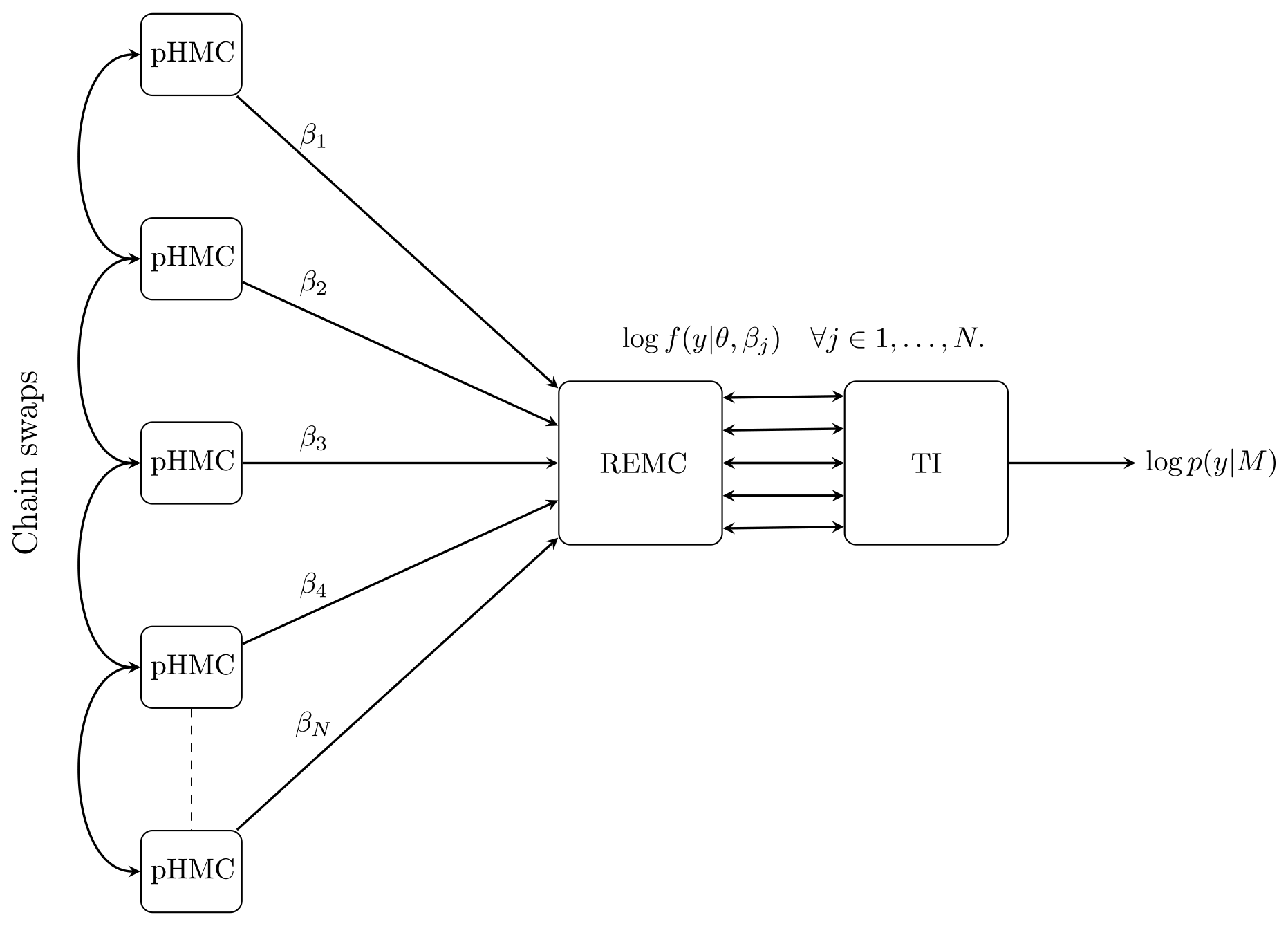
Figure 2 Overall schematic of the REHMC + TI algorithm for estimating the marginal likelihood for a given model M. Working from left to right, N pHMC samplers are run at different values of the inverse temperature parameter $\left\{{\mathit{\beta }}_{\mathrm{1}},{\mathit{\beta }}_{\mathrm{2}},\mathrm{\dots },{\mathit{\beta }}_N\right\}$ with $\mathrm{0}\le {\mathit{\beta }}_j\le \mathrm{1},j=\mathrm{1},\mathrm{\dots },N,$ to simulate from the power posterior $\log f(y;{\mathit{\theta }}_i,{\mathit{\beta }}_j)$. The REMC algorithm is responsible for swapping the state between adjacent chains according to the Metropolis–Hastings criteria. Finally, the TI methodology is used to calculate an estimate of the marginal likelihood log p(y|M). Note that in terms of setup, information flows from right to left; i.e. the discretization of the TI integral is responsible for setting the number (N) and values of inverse temperatures (${\mathit{\beta }}_{\mathrm{1}},\mathrm{\dots },{\mathit{\beta }}_N$).

2.3.1 Thermodynamic integration

Thermodynamic integration (TI) has its origins in theoretical physics, where it is used to calculate free energy differences between systems (Torrie and Valleau, 1977) before appearing in the statistical literature as path sampling (Gelman and Meng, 1998), a method for calculating marginal likelihoods. TI converts a high-dimensional integral into a one-dimensional integration problem over a unit interval.

To derive the TI estimate of the marginal likelihood p(y), we first raise the likelihood to the power of $\mathrm{0}\le \mathit{\beta }\le \mathrm{1}$ to form the power posterior (Friel and Pettitt, 2008):

$$\begin{array}{}\text{(9)}& {\mathit{\pi }}_{\mathrm{power}}\left(\mathit{\theta }\right|y,\mathit{\beta })={\displaystyle \frac{\left[f\right(y\left|\mathit{\theta }\right){]}^{\mathit{\beta }}\mathit{\pi }\left(\mathit{\theta }\right)}{p\left(y\right|\mathit{\beta })}},\end{array}$$

with

$$\begin{array}{}\text{(10)}& p\left(y\right|\mathit{\beta })=\int [f\left(y\right|\mathit{\theta }\left){]}^{\mathit{\beta }}\mathit{\pi }\right(\mathit{\theta })\mathrm{d}\mathit{\theta }.\end{array}$$

When β=0, the power posterior is the same as the prior distribution. When β=1, we have the standard posterior distribution. This makes a continuous path between the prior and posterior distributions.

Taking the logarithm on both sides of Eq. (10) and using the chain rule, a differentiation with respect to β yields

$$\begin{array}{}\text{(11)}& \begin{array}{rl}{\displaystyle \frac{\partial }{\partial \mathit{\beta }}}\log p\left(y\right|\mathit{\beta })& ={\displaystyle \frac{\mathrm{1}}{p\left(y\right|\mathit{\beta })}}{\displaystyle \frac{\partial }{\partial \mathit{\beta }}}p\left(y\right|\mathit{\beta })\\ & ={\displaystyle \frac{\mathrm{1}}{p\left(y\right|\mathit{\beta })}}\int {\displaystyle \frac{\partial }{\partial \mathit{\beta }}}\left[f\right(y\left|\mathit{\theta }\right){]}^{\mathit{\beta }}\mathit{\pi }\left(\mathit{\theta }\right)\mathrm{d}\mathit{\theta }\\ & ={\displaystyle \frac{\mathrm{1}}{p\left(y\right|\mathit{\beta })}}\int \left[f\right(y\left|\mathit{\theta }\right){]}^{\mathit{\beta }}\log f\left(y\right|\mathit{\theta }\left)\mathit{\pi }\right(\mathit{\theta })\mathrm{d}\mathit{\theta }\\ & =\int {\displaystyle \frac{\left[f\right(y\left|\mathit{\theta }\right){]}^{\mathit{\beta }}\mathit{\pi }\left(\mathit{\theta }\right)}{p\left(y\right|\mathit{\beta })}}\log f\left(y\right|\mathit{\theta })\mathrm{d}\mathit{\theta }\\ & ={\mathbb{E}}_{p\left(\mathit{\theta }\right|y,\mathit{\beta })}\left[\log f\right(y\left|\mathit{\theta }\right)],\end{array}\end{array}$$

where ${\mathbb{E}}_{p\left(\mathit{\theta }\right|y,\mathit{\beta })}$ is the expectation with respect to the power posterior. Integrating both sides of equation (Eq. 11) with respect to β gives the log of the marginal likelihood of interest, p(y), in terms of an integral of β:

$$\begin{array}{}\text{(12)}& \log p\left(y\right)=\underset{\mathrm{0}}{\overset{\mathrm{1}}{\int }}{\mathbb{E}}_{p\left(\mathit{\theta }\right|y,\mathit{\beta })}\left[\log f\right(y\left|\mathit{\theta }\right)]\mathrm{d}\mathit{\beta },\end{array}$$

This manipulation allows us to find a way to approximate the value of p(y). Computationally, posterior samples are drawn for each value of β. The values are then evaluated in the log likelihood, and the mean for each value of β is obtained. The integral in Eq. (12) on β can be estimated using the trapezoidal rule as follows:

$$\begin{array}{rl}\log p\left(y\right)& =\sum _{j=\mathrm{1}}^N{\displaystyle \frac{({\mathit{\beta }}_j-{\mathit{\beta }}_{j-\mathrm{1}})}{\mathrm{2}}}\left[{\mathbb{E}}_{p\left(\mathit{\theta }\right|y,{\mathit{\beta }}_j)}\log f\left(y\right|\mathit{\theta })\right.\\ & \left.+{\mathbb{E}}_{p\left(\mathit{\theta }\right|y,{\mathit{\beta }}_{j-\mathrm{1}})}\log f\left(y\right|\mathit{\theta })\right].\end{array}$$

The Monte Carlo estimate of the expectations can then be obtained by

$$\begin{array}{}\text{(13)}& \begin{array}{rl}\log p\left(y\right)& \approx \sum _{j=\mathrm{1}}^N{\displaystyle \frac{({\mathit{\beta }}_j-{\mathit{\beta }}_{j-\mathrm{1}})}{\mathrm{2}}}\left[{\displaystyle \frac{\mathrm{1}}{S}}\sum _{i=\mathrm{1}}^S\log f\left(y\right|{\mathit{\theta }}_i,{\mathit{\beta }}_j)\right.\\ & \left.+{\displaystyle \frac{\mathrm{1}}{S}}\sum _{i=\mathrm{1}}^S\log f\left(y\right|{\mathit{\theta }}_i,{\mathit{\beta }}_{j-\mathrm{1}})\right],\end{array}\end{array}$$

where $j=\mathrm{1},\mathrm{\dots },N$ is the index for the β values and S is the number of posterior samples for each β value. The accuracy of the TI estimate depends on the integration rule on β, i.e. the number of β values and the spacing of the values, and the convergence of the Markov chain Monte Carlo (MCMC). The most commonly employed path is a geometric path (Calderhead and Girolami, 2009):

$$\begin{array}{}\text{(14)}& {\mathit{\beta }}_j={\left({\displaystyle \frac{j}{N}}\right)}^{\mathrm{5}},j=\mathrm{1},\mathrm{\dots },N.\end{array}$$

The number of β_j values can be adaptively chosen as a tradeoff between model convergence and computational efficiency, for instance, see Vousden et al. (2016). The complete TI algorithm is presented in Algorithm 1.

Algorithm 1 Thermodynamic integration (TI).

Require:

β {$\mathit{\beta }=\mathit{\{}\mathrm{1},\mathrm{\dots },\mathrm{0}\mathit{\}}$ : schedule of inverse temperatures based on the trapezoidal rule of size N, and S is the number of samples per replica.}

Ensure:

Log marginal likelihood (log p(y)).

1:

REpHMC(β) {Run a single step of the REpHMC algorithm S times; see Sect. 2.3.2.}

2:

Estimate log p(y) by the definition of the quadrature rule, e.g. trapezoidal rule

$$\begin{array}{rl}\log p\left(y\right)& \approx \sum _{j=\mathrm{1}}^N{\displaystyle \frac{({\mathit{\beta }}_j-{\mathit{\beta }}_{j-\mathrm{1}})}{\mathrm{2}}}\left[{\displaystyle \frac{\mathrm{1}}{S}}\sum _{i=\mathrm{1}}^S\log f\left(y\right|{\mathit{\theta }}_i,{\mathit{\beta }}_j)\right.\\ & \left.+{\displaystyle \frac{\mathrm{1}}{S}}\sum _{i=\mathrm{1}}^S\log f\left(y\right|{\mathit{\theta }}_i,{\mathit{\beta }}_{j-\mathrm{1}})\right].\end{array}$$

2.3.2 Replica-exchange Monte Carlo

The REMC algorithm was introduced by Swendsen and Wang (1986). Geyer (1991) presented a similar formulation to the statistical community under the name Metropolis-coupled MCMC. REMC is a generic algorithm in that it can be combined with other algorithms. Miasojedow et al. (2013) combined REMC with random walk Metropolis (RWM). RWM is a gradient-free algorithm in that it generates posterior samples from the target distribution by randomly sampling from a proposal distribution. We combine REMC with HMC, which gives the new algorithm, REHMC, explained in the rest of this section. When REMC is combined with pHMC, we get the REpHMC. The REpHMC gives a higher effective sample size than REHMC. The effective sample size is the number of independent samples with the same amount of information as correlated samples. Each sample in a Markov chain is correlated to the preceding sample, so the samples have less information than independent samples. The effective sample size takes into account this autocorrelation. The main idea of REMC is that an ensemble of power posterior chains, known as replicas, run in parallel. The likelihood of these chains is raised to values from 0 to 1. These values are called inverse temperatures. Each replica performs a Metropolis update to get the next value at each iteration. Adjacent replica pairs are randomly selected, and an attempt is made to swap the current values of the replica pairs. A swap is accepted or rejected according to the Metropolis–Hastings algorithm. The swapping accelerates convergence to the target distribution, avoids chains becoming trapped in topologically isolated areas of the parameter space, and improves the mixing of the chains. REMC is also known as parallel tempering (Hansmann, 1997; Earl and Deem, 2005). When the method has an iterated importance sampling step, it is known as population Monte Carlo (PMC) (Iba, 2000; Cappé et al., 2004). However, the term PMC has also been used for methods without an importance sampling step (Calderhead and Girolami, 2009; Friel and Pettitt, 2008; Mingas and Bouganis, 2016).

The REpHMC is summarized in Algorithm 2. We emphasize that the samples of the replica with β=1 are used to estimate the posterior parameters, while the entire ensemble is used as input within TI to calculate the marginal likelihood.

Algorithm 2 Single step of replica-exchange preconditioned Hamiltonian Monte Carlo (REpHMC).

Require:

L, ϵ, θ^t, β {L: number of leapfrog steps, ϵ: leapfrog step size, ${\mathit{\theta }}^t=\mathit{\{}{\mathit{\theta }}_{\mathrm{1}}^t,\mathrm{\dots },{\mathit{\theta }}_N^t\mathit{\}}$: initial values for each β, $\mathit{\beta }=\mathit{\{}{\mathit{\beta }}_{\mathrm{1}},\mathrm{\dots },{\mathit{\beta }}_N\mathit{\}}$: schedule of N inverse temperatures}

Ensure:

$({\mathit{\theta }}_{\mathrm{1}}^{t+\mathrm{1}},\mathrm{\dots },{\mathit{\theta }}_N^{t+\mathrm{1}})$ {Posterior samples for each β}.

1:

for i=1 to N do

2:

${\mathit{\theta }}_i^{t+\mathrm{1}}\leftarrow \mathrm{pHMC}(L,\mathit{ϵ},{\mathit{\theta }}_i^t)$ {Run single step of pHMC algorithm on each replica}

3:

end for

4:

for i=1 to N−1 do

5:

$j\leftarrow i+\mathrm{1}$ {Select adjacent chain}

6:

$\mathit{\alpha }\leftarrow \min (\mathrm{1},{\displaystyle \frac{{\mathit{\pi }}_i\left({\mathit{\theta }}_j^{t+\mathrm{1}}\right){\mathit{\pi }}_j\left({\mathit{\theta }}_i^{t+\mathrm{1}}\right)}{{\mathit{\pi }}_i\left({\mathit{\theta }}_i^{t+\mathrm{1}}\right){\mathit{\pi }}_j\left({\mathit{\theta }}_j^{t+\mathrm{1}}\right)}})$ {where, for example, π_i(⋅) is the power posterior associated with temperature β_i}.

7:

$u\sim U(\mathrm{0},\mathrm{1})$

8:

if u≤α then

9:

(${\mathit{\theta }}_i^{t+\mathrm{1}},{\mathit{\theta }}_j^{t+\mathrm{1}})\leftarrow ({\mathit{\theta }}_j^{t+\mathrm{1}},{\mathit{\theta }}_i^{t+\mathrm{1}}$)

10:

else

11:

(${\mathit{\theta }}_i^{t+\mathrm{1}},{\mathit{\theta }}_j^{t+\mathrm{1}})\leftarrow ({\mathit{\theta }}_i^{t+\mathrm{1}}$, ${\mathit{\theta }}_j^{t+\mathrm{1}}$)

12:

end if

13:

end for

Like any sampling method, the REpHMC's convergence should be assessed. We used both trace plots and formal diagnostic tests to check for convergence of the Markov chain since there is no universal robust test for convergence (Cowles and Carlin, 1996). The most widely used method to assess the convergence of Markov chains is the potential scale reduction factor $\widehat{R}$ developed by Gelman and Rubin (1992) and extended by Brooks and Gelman (1998). Recently, an improved factor $\widehat{R}$ was proposed by Vehtari et al. (2021). For $\widehat{R}$ to be a valid statistic, the chains must be independent of each other. In REpHMC, the chains are not independent due to swapping. Therefore, we used methods that require one chain or replica per temperature – namely, the Geweke diagnostic (Geweke, 1992) and the integrated autocorrelation time (IAT) (Geyer, 1992; Kendall et al., 2005). For the sake of brevity, we do not explain these concepts here but instead refer the reader to the respective papers.

2.3.3 Hamiltonian Monte Carlo

HMC is a gradient-based technique used to sample from a continuous probability density (Duane et al., 1987). HMC scales better in high dimensions than gradient-free samplers, such as nested sampling, due to the inclusion of derivative information (Ashton et al., 2022). Therefore, many applications combine HMC and gradient-free samplers. For example, Elsheikh et al. (2014) have combined HMC and nested sampling. HMC is based on the Hamiltonian, which describes a particle's position and momentum at any time. New positions are known by solving Hamilton's equations of motion for position and momentum. In Bayesian inference, the Hamiltonian H(θ,ρ) in Eq. (15) describes the evolution of a d-dimensional vector (θ) of parameters and a corresponding d-dimensional vector of auxiliary momentum (ρ) variables at any time t.

$$\begin{array}{}\text{(15)}& \begin{array}{rl}{\displaystyle }H(\mathit{\theta },\mathit{\rho })& {\displaystyle }=-\log f\left(y\right|\mathit{\theta }\left)\mathit{\pi }\right(\mathit{\theta })+{\displaystyle \frac{\mathrm{1}}{\mathrm{2}}}{\mathit{\rho }}^T\mathbf{M}\mathit{\rho }\\ {\displaystyle }& {\displaystyle }=U\left(\mathit{\theta }\right)+K\left(\mathit{\rho }\right)\end{array}\end{array}$$

In Eq. (15), M is the positive definite mass matrix. U(θ) is the desired posterior known as potential energy, and K(ρ) is the kinetic energy that is a function of momentum. To sample from the Hamiltonian, we take the partial derivatives, which give Hamilton's equations of motion:

$$\begin{array}{}\text{(16a)}& {\displaystyle \frac{\mathrm{d}\mathit{\theta }}{\mathrm{d}t}}& {\displaystyle }={\displaystyle \frac{\partial H}{\partial \mathit{\rho }}}={\displaystyle \frac{\partial K}{\partial \mathit{\rho }}},\text{(16b)}& {\displaystyle \frac{d\mathit{\rho }}{\mathrm{d}t}}& {\displaystyle }=-{\displaystyle \frac{\partial H}{\partial \mathit{\theta }}}=-{\displaystyle \frac{\partial U}{\partial \mathit{\theta }}}.\end{array}$$

We now have a system of ODEs (Eqs. 16a to 16b). The leapfrog method (Duane et al., 1987; Radford, 2011) is used to solve Eqs. (16a) to (16b) and propose new values for the parameters. The accuracy of the leapfrog method depends on discretization step ϵ.

Each HMC iteration consists of two steps (Radford, 2011). In the first step, the momentum values for each parameter are sampled from a Gaussian distribution independent of the current θ values, ${\mathit{\rho }}^{*}\sim \mathrm{MVN}(\mathrm{0},\mathbf{M})$. Then, using the current parameter and momentum values, (θ^t,ρ^t), the Hamiltonian is simulated using an appropriate time-stepping method, such as the leapfrog method (Betancourt, 2017). At the end of Hamiltonian dynamics, the momentum values are negated, and the new parameter values $({\mathit{\theta }}^{*},{\mathit{\rho }}^{*})$ are accepted or rejected using the Metropolis–Hastings criterion with acceptance probability α, where

$$\begin{array}{}\text{(17)}& \mathit{\alpha }=min\left[\mathrm{1},\exp \left(-U\left({\mathit{\theta }}^{*}\right)+U\left({\mathit{\theta }}^t\right)-K\left({\mathit{\rho }}^{*}\right)+K\left({\mathit{\rho }}^t\right)\right)\right].\end{array}$$

The HMC is summarized in Algorithm 3. The mixing of the HMC chain depends on the number of leapfrog steps, L, and step size ϵ. L and ϵ can be automatically tuned during the warm-up phase of the algorithm (Hoffman and Gelman, 2014). The warm-up phase is the period during which posterior samples are discarded and is also called burn-in. In this work, ϵ was automatically tuned by the dual averaging algorithm, while L was manually tuned. Dual averaging automatically adjusts ϵ during the warm-up of the HMC algorithm until a specific acceptance rate is achieved. We used an acceptance rate of 0.75, which is higher than the optimal acceptance rate of RWM-based algorithms. This is the mean of various reported values and the default in TensorFlow probability. To increase the sampling efficiency of HMC, we have to reduce the correlation of the parameters, especially for ODE models. This is achieved by introducing a preconditioned matrix, M, and hence the name is pHMC. This leads to even faster convergence and higher effective sample sizes for each parameter (Girolami and Calderhead, 2011). In practice, the preconditioned matrix is the inverse of the covariance matrix of the target posterior. In contrast to HMC, where the momentum is sampled from a normal distribution, for pHMC, the momentum values are sampled from a multivariate Gaussian distribution with a covariance matrix as the preconditioned matrix, $\mathit{\rho }\sim \text{MVN}(\mathrm{0},\mathbf{M})$. The covariance matrix controls the correlation of the parameters. The rest of the algorithm for pHMC works in the same way as for HMC.

Algorithm 3 A single step of preconditioned Hamiltonian Monte Carlo (pHMC), with notation following Radford (2011).

Require:

$L,\mathit{ϵ},{\mathit{\theta }}^t$ {L: number of leapfrog steps, ϵ: leapfrog step size, θ^t: initial value.}

Ensure:

θ^t+1

1:

${\mathit{\rho }}^{*}\sim \mathrm{MVN}(\mathrm{0},\mathbf{M})$ {Sample momentum values, and M is the mass matrix}

2:

${\mathit{\theta }}^{*}\leftarrow {\mathit{\theta }}^t$

3:

for i=1 to L do

4:

$({\mathit{\theta }}^{\mathit{ϵ}},{\mathit{\rho }}^{\mathit{ϵ}})\leftarrow \mathrm{leapfrog}(\mathit{\theta },\mathit{\rho },\mathit{ϵ})$

5:

end for

6:

${\mathit{\rho }}^{*}\leftarrow -{\mathit{\rho }}^{*}$

7:

$\mathit{\alpha }\leftarrow min\left(\mathrm{1},\exp \left(-U\left({\mathit{\theta }}^{*}\right)+U\left({\mathit{\theta }}^t\right)-K\left({\mathit{\rho }}^{*}\right)+K\left({\mathit{\rho }}^t\right)\right)\right)$

8:

$u\sim U(\mathrm{0},\mathrm{1})$

9:

if u≤α then

10:

${\mathit{\theta }}^{t+\mathrm{1}}\leftarrow {\mathit{\theta }}^{*}$

11:

else

12:

${\mathit{\theta }}^{t+\mathrm{1}}\leftarrow {\mathit{\theta }}^t$

13:

end if

14:

15:

function leapfrog($\mathit{\theta },\mathit{\rho },\mathit{ϵ}$) {Solves the equations to propose new values}

16:

${\mathit{\rho }}^{\mathit{ϵ}/\mathrm{2}}\leftarrow \mathit{\rho }-\frac{\mathit{ϵ}}{\mathrm{2}}\frac{\partial U}{\partial \mathit{\theta }}\left(\mathit{\theta }\right)$

17:

${\mathit{\theta }}^{\mathit{ϵ}}\leftarrow \mathit{\theta }+\mathit{ϵ}\mathbf{M}{s}^{-\mathrm{1}}{\mathit{\rho }}^{\mathit{ϵ}/\mathrm{2}}$

18:

${\mathit{\rho }}^{\mathit{ϵ}}\leftarrow {\mathit{\rho }}^{\mathit{ϵ}/\mathrm{2}}-\frac{\mathit{ϵ}}{\mathrm{2}}\frac{\partial U}{\partial \mathit{\theta }}\left({\mathit{\theta }}^{\mathit{ϵ}}\right)$

19:

return (θ^ϵ,ρ^ϵ)

2.4 Implementation aspects

In this section, we outline some of the more non-standard aspects of implementing the proposed methodology in the probabilistic programming language (PPL) TFP. Probabilistic programming (PP) is a methodology for performing computational statistical modelling in which all elements of the Bayesian joint posterior $\mathit{\pi }\left(\mathit{\theta }\right|y,M)$ are specified in a PPL. Popular PPLs include Stan (Carpenter et al., 2017), PyMC3 (Salvatier et al., 2016), and TFP (Dillon et al., 2017). Once specified in a PPL, the subsequent Bayesian parameter inference problem can then be handled semi-automatically. We refer the reader to the “Code and data availability” section for the full implementation and simply remark that the joint posterior for our problem can be defined in around 70 lines of TFP/JAX code.

We choose to use TFP in this study. From our experience, TFP is the most flexible and extensible PPL in terms of allowing advanced model specification and the ability to break out of the high-level interface and perform low-level operations. However, this flexibility comes at the cost of a steeper learning curve, particularly TFP’s complex batch and event shape semantics (Dillon et al., 2017). We note that despite TensorFlow in the name, TFP is backend agnostic and can run on top of various differentiable programming languages. We choose to run TFP on top of JAX, instead of the default choice of TensorFlow. Anecdotally, our experience is that TFP on JAX has better runtime performance and is more robust than TFP on TensorFlow, particularly when working with ODE-based models. We use JAX with the CPU backend and double-precision floating point representation, although in principle the GPU backend could also be used. TFP already includes an implementation of the HMC and REMC algorithms, the output of which can be used with TI for computing the marginal likelihood.

JAX can automatically perform arbitrarily composable forward- and backward-mode automatic differentiation of nearly arbitrary computer programs. This is used to automatically differentiate the TFP specification of the negative log posterior U(θ) with respect to the model parameter θ for use within the HMC algorithm. As this approach is now standard, we refer the reader to Margossian (2019) for a detailed review.

For the automatic differentiation of the ODE model, we use the continuous adjoint approach. This approach is also called continuous backpropogation in the neural ODE literature; see, for example, Kelly et al. (2020) and Höge et al. (2022) for an application in hydrology. We follow the presentation in Kidger (2021), where a new set of adjoint ODEs is from the original continuous ODE system. This adjoint system is then discretized (backwards in time) using the same ODE solver as for Eq. (1), an explicit adaptive Dormand–Prince ODE integrator that is already included in JAX. It is worth remarking that while the continuous adjoint system is still derived automatically within JAX, the result is distinctly different to backwards differentiation through the steps of the forward ODE solver at the programmatic level. For more details, we refer the reader to Kidger (2021) for a discussion of the different methods for automatically differentiating ODE systems and their relative tradeoffs.

Let V be the solution to Eq. (1). In the simplest case, let J=J(V(T)) be some scalar function of the terminal solution value V(T) (the approach extends straightforwardly to other functionals). Setting $\frac{\mathrm{d}J}{\mathrm{d}V}=a_V\left(t\right)$ and $\frac{\mathrm{d}J}{\mathrm{d}\mathit{\theta }}=a_{\mathit{\theta }}\left(\mathrm{0}\right)$ where $a_V:[\mathrm{0},T]\to {\mathbb{R}}^n$ and $a_{\mathit{\theta }}:[\mathrm{0},T]\to {\mathbb{R}}^p$ are the solutions to the following adjoint ODE system:

$$\begin{array}{}\text{(18a)}& {\displaystyle }(a_V{)}_t=-a_V(t{)}^T{\displaystyle \frac{\partial f}{\partial V}}(t,V,\mathit{\theta }),a_V\left(T\right)={\displaystyle \frac{\mathrm{d}J}{\mathrm{d}V\left(T\right)}},\text{(18b)}& {\displaystyle }(a_{\mathit{\theta }}{)}_t=-a_V(t{)}^T{\displaystyle \frac{\partial f}{\partial \mathit{\theta }}}(t,V,\mathit{\theta }),a_{\mathit{\theta }}\left(T\right)=\mathrm{0}.\end{array}$$

Note that the adjoint system requires the forward solution to have already been computed and that the adjoint system runs backwards in time, i.e. evolving from known states a_V(T) and a_θ(T) at terminal time t=T to the starting time t=0. Once a_θ(0) has been computed, the required gradient of the functional $\frac{\mathrm{d}J}{\mathrm{d}\mathit{\theta }}=a_{\mathit{\theta }}\left(\mathrm{0}\right)$ can be computed straightforwardly. This continuous adjoint ODE approach can be arbitrarily composed with JAX's programme level automatic differentiation capabilities, meaning that it is possible to add non-ODE-based components (e.g. smoothers) to the model and use our framework for computing marginal likelihoods.

3 Results and discussion

The purpose of this section is to test the accuracy of REpHMC in calculating the BF by employing it to solve benchmark problems with complex distributions but well-known log marginal likelihoods and thus the BF. We illustrate that the BF can distinguish between models with an equally good fit by calculating the BF of synthetic discharge data for three different models, among which is the data-generating model. We repeat the experiment using another data-generating model. Finally, the BF is applied to the real-world discharge data.

3.1 Gaussian shell example

This section aims to show that the proposed methodology accurately estimates the marginal likelihood of a synthetic example. In addition, it illustrates the effectiveness of REpHMC in sampling multimodal distributions. The benchmark example is the Gaussian shells (Feroz et al., 2009; Allanach and Lester, 2008). This example has two wholly separated Gaussian shells, making it difficult to sample from. This example has been used to test various techniques for calculating the marginal likelihood (Thijssen et al., 2016; Henderson and Goggans, 2019). The Gaussian shell likelihood is given as

$$\begin{array}{}\text{(19)}& \begin{array}{rl}\mathrm{\ell }\left(\mathit{\theta }\right)& ={\displaystyle \frac{\mathrm{1}}{\sqrt{\mathrm{2}\mathit{\pi }{w}_{\mathrm{1}}^{\mathrm{2}}}}}\exp [-{\displaystyle \frac{(\Vert {\mathit{\theta }}_{\mathrm{1}}-c_{\mathrm{1}}\Vert -r_{\mathrm{1}}{)}^{\mathrm{2}}}{\mathrm{2}{w}_{\mathrm{1}}^{\mathrm{2}}}}]\\ & +{\displaystyle \frac{\mathrm{1}}{\sqrt{\mathrm{2}\mathit{\pi }{w}_{\mathrm{2}}^{\mathrm{2}}}}}\exp [-{\displaystyle \frac{(\Vert {\mathit{\theta }}_{\mathrm{2}}-c_{\mathrm{2}}\Vert -r_{\mathrm{2}}{)}^{\mathrm{2}}}{\mathrm{2}{w}_{\mathrm{2}}^{\mathrm{2}}}}].\end{array}\end{array}$$

The unknown parameters are θ=(θ₁, θ₂), while the marginalized fixed parameters are $r_{\mathrm{1}},r_{\mathrm{2}},w_{\mathrm{1}},w_{\mathrm{2}},c_{\mathrm{1}}$, and c₂. The first shell has a radius of r₁ and the second shell of r₂. The first shell is centred at c₁, while the second is centred at c₂. The variance (width) of the first shell is w₁ and that of shell 2 is w₂. We assign uniform priors to θ₁ and θ₂ in the range from −6 to 6, and the marginalized parameters are set to $w_{\mathrm{1}}=w_{\mathrm{2}}=\mathrm{0.1}$, $r_{\mathrm{1}}=r_{\mathrm{2}}=\mathrm{2}$, c₁=3.5, and $c_{\mathrm{2}}=-\mathrm{3.5}$. We used 26 temperature schedules since it is a difficult sampling problem to obtain fast mixing due to the two regions of probability mass. The convergence of the number of temperatures was checked after the convergence of the posterior samples. The log marginal likelihood is stable after using 22 temperatures. From this point, there is very little variation in the log marginal likelihood, as shown in Fig. 3. The plot shows that the log marginal likelihood is constant from 10 to 11 temperatures. Although 10 temperatures are commonly used, this would have underestimated the actual value. To assess convergence, diagnostic plots were made by running the same temperature schedules twice in parallel with two different random initial parameter values, and the results are displayed in Fig. 3, where the horizontal red line is the true value. The swap acceptance rate ranges from 0.389 for 10 temperature schedules to 0.479 for more than 50 temperatures.

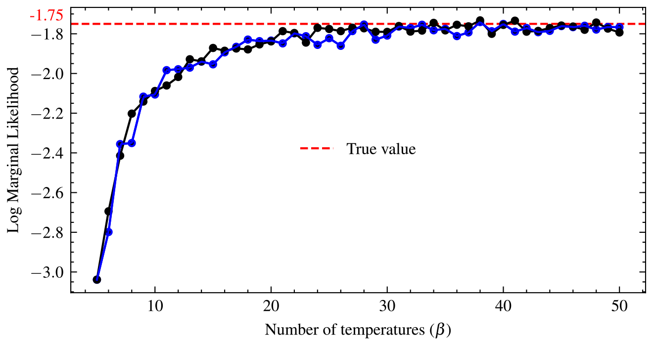
Figure 3 Convergence diagnostic plots of the log marginal likelihood for the Gaussian shell in two dimensions. The temperature schedules is run twice in parallel with random initial parameter values. Convergence occurs when the curves plateau.

A plot of the samples for the parameters using various samplers is shown in Fig. 4. The plot demonstrates that due to the addition of replica exchange the REpHMC method can sample across the shells compared to algorithms such as NUTS (Hoffman and Gelman, 2014), MALA (Xifara et al., 2014), or plain HMC (not shown), which are purely local. The results of the marginal likelihood up to 30 dimensions are shown in Table 2, with agreement with the marginal likelihood values reported in the literature (Feroz et al., 2009).

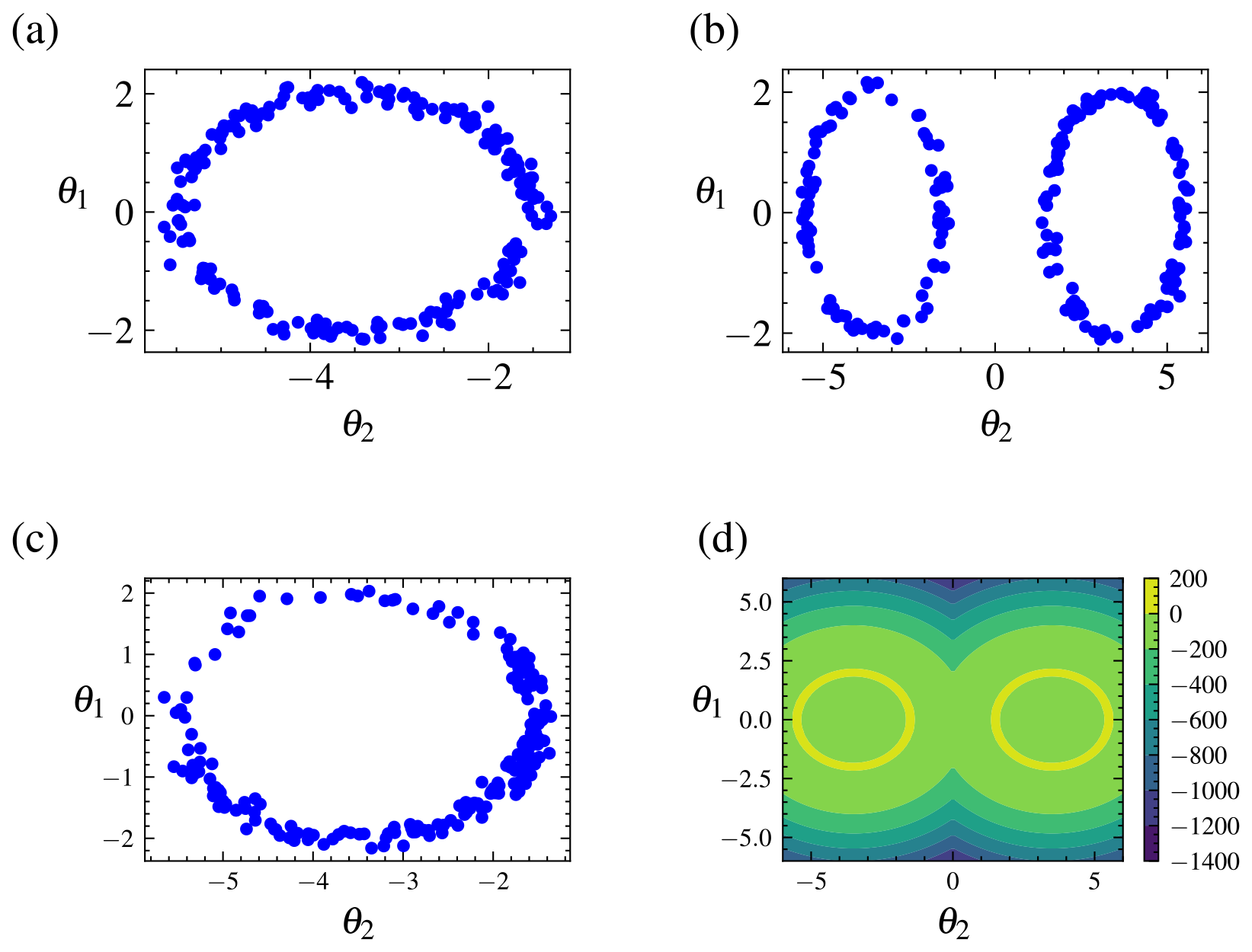
Figure 4 Posterior samples for the Gaussian shell example obtained by different algorithms alongside the target distribution. Top left (a) is NUTS, top right (b) is REpHMC, bottom left (c) is MALA, and bottom right (d) is the target distribution. Because of the addition of replica exchange, REpHMC can sample across the entire distribution space. This is in contrast to the NUTS, MALA, and HMC (not shown) samplers which cannot transition across the gap between the two shells.

Table 2 Log marginal likelihood (log p(y)) of the Gaussian shell example. The true values are shown, and the estimates are based on thermodynamic integration with samples from REpHMC. The results are shown for up to 30 dimensions.

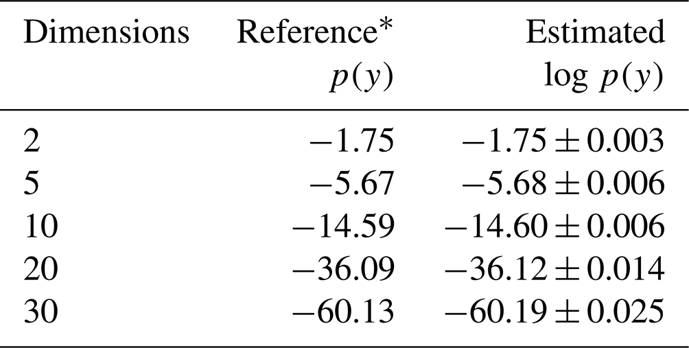
^* As reported in Feroz et al. (2009).

3.2 Synthetic examples

In this section, we generate synthetic discharge data using the observed precipitation and observed potential evapotranspiration as inputs to our models. The following two examples aim to verify the correct implementation and study the behaviour of the methodology to calculate the marginal likelihood. In the first experiment, data y_obs is generated from the simplest model, M₂. In the second experiment, M₃ (three-bucket model) is the data-generating model. For each experiment, the log marginal likelihood log p(y|M_i) for $i=\mathrm{2},\mathrm{3},\mathrm{4}$ and the respective Bayes factors are calculated. The deviance information criterion (DIC) and widely applicable information criterion (WAIC) are also calculated for experiments in Sect. 3.2.1 and 3.2.2 and for real-world discharge data in Sect. 3.3.

3.2.1 Experiment 1 with data generated from the two-bucket model, M₂

In the first experiment, synthetic discharge data y_obs is generated from the simplest model, M₂ (two-bucket model) to see if the BF will select M₂. We set up the priors as in Table 3. The synthetic discharge is generated to have similar dynamics as the observed discharge shown in Fig. 5. First, we obtain the daily precipitation and evapotranspiration for the Magela Creek catchment in Australia for 1980. The initial time, t=0, corresponds to midnight on 1 January 1980, and the final time, T=366 d, to midnight on 31 December 1980 (1980 was a leap year). It is assumed that the total precipitation and evapotranspiration on a given day are uniformly distributed over the 24 h from midnight to midnight. This is an acceptable assumption when modelling the dynamics of a catchment on a multiday timescale.

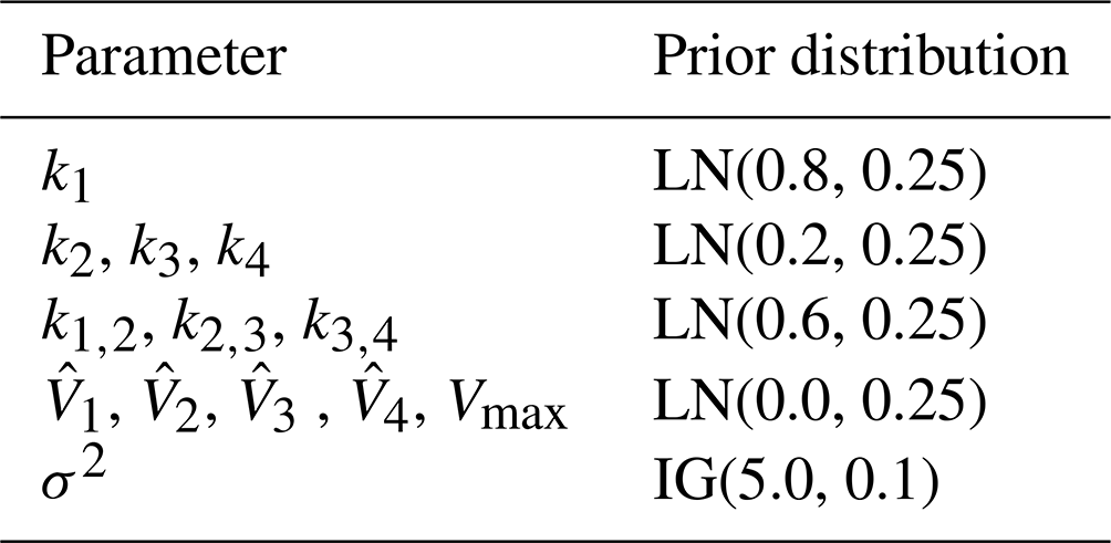
Table 3 Description of the parameters and priors. Note that here we have used units more common in the hydrological literature. LN is the lognormal distribution and IG is the inverse gamma distribution. The IG was chosen because it is easier to sample than other distributions for the prior noise parameter, which must be positive.

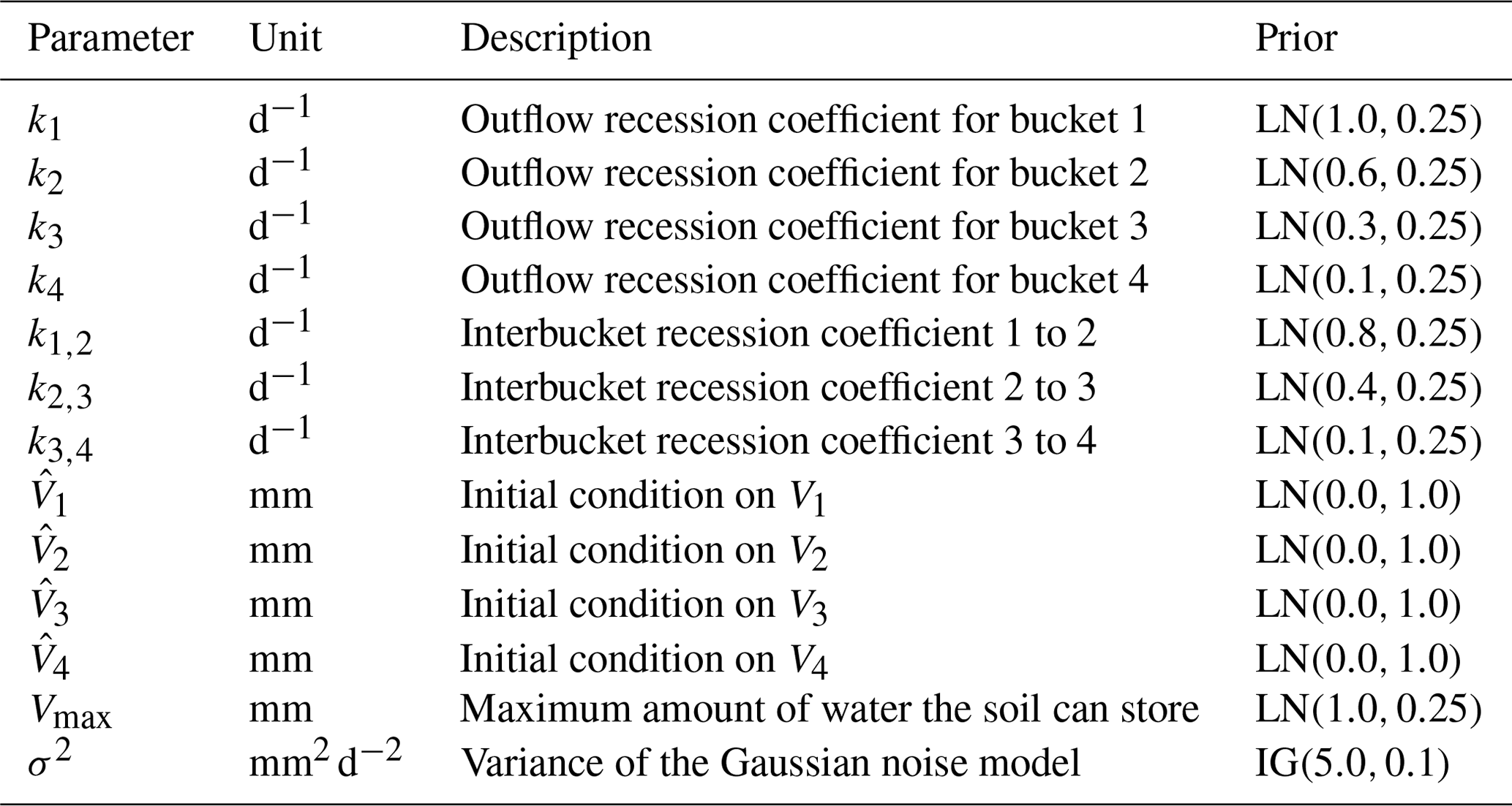
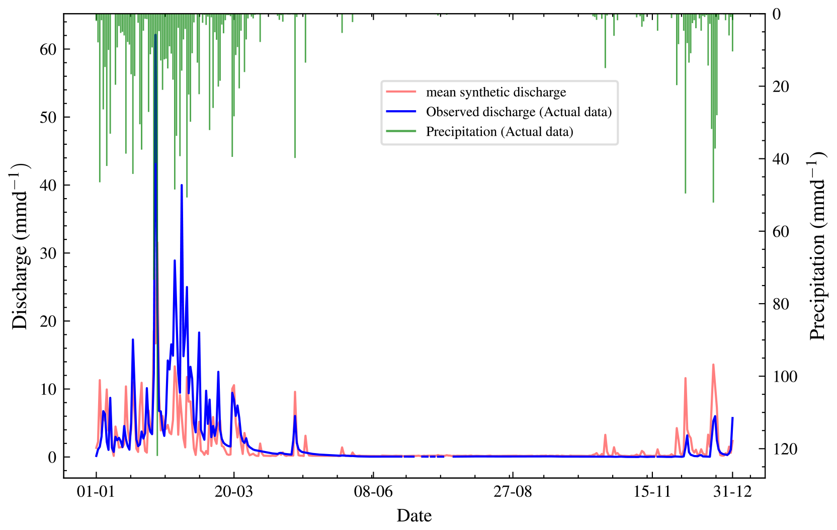
Figure 5 Plot of observed discharge, synthetic discharge, and precipitation from 1 January to 31 December 1980. The observed discharge has missing values, represented by the broken blue line, mostly in the seventh month. Synthetic discharge data generated via the joint posterior (before calibration) shows similar overall trends to the observed discharge.

Our analysis focuses on a 3-month period in 1980 running from 1 January to 31 March 1980 when the precipitation frequency is the highest, and there are no missing data.

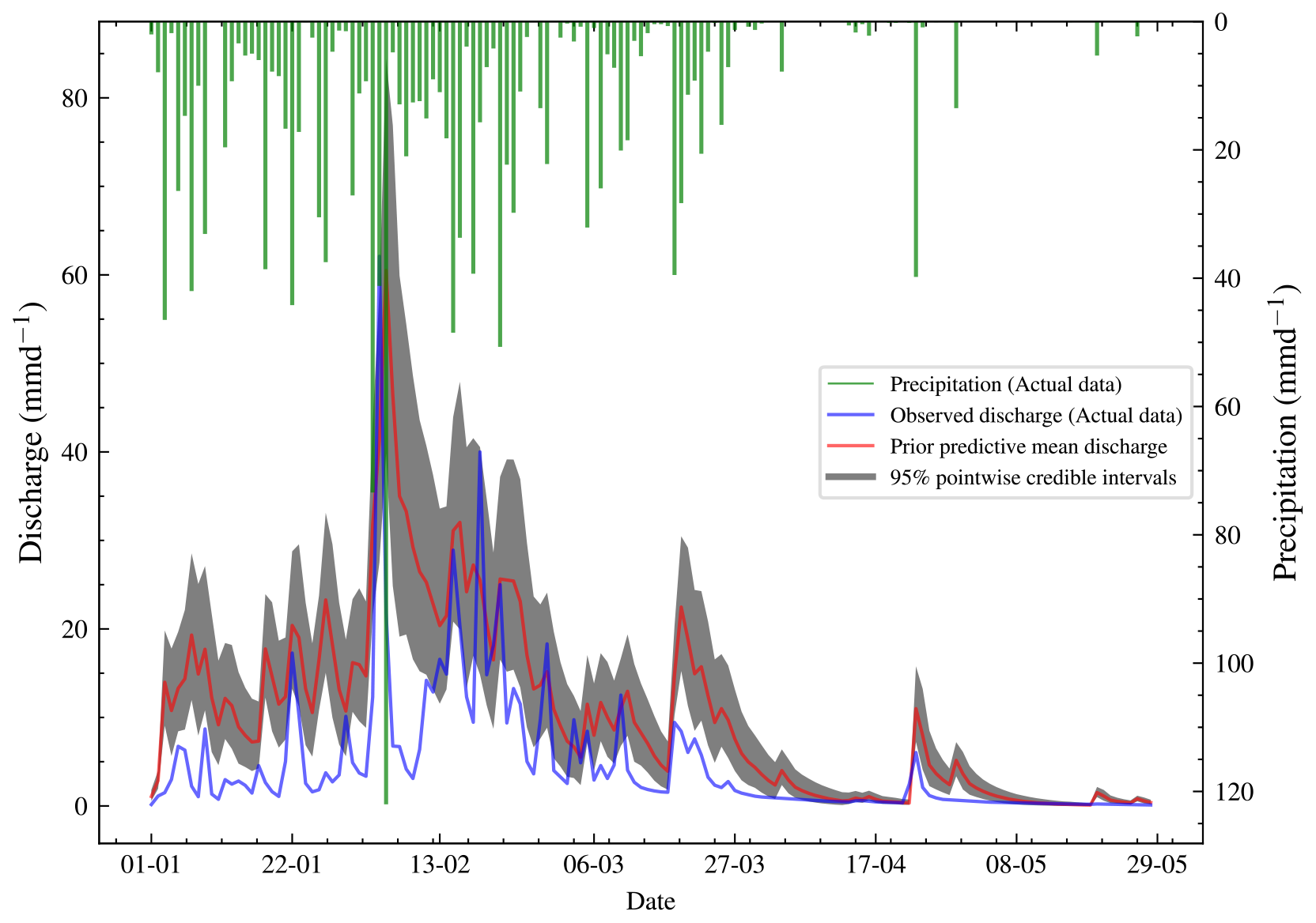
Figure 6 Plot of observed discharge, synthetic discharge, and precipitation from 1 January to 29 May 1980. This period has no missing values and has the highest precipitation frequency and discharge of the year 1980. The synthetic discharge has a similar trend to the observed discharge. The synthetic discharge here is generated using a different set of parameters compared to that in Fig. 5.

We set up the priors according to the following reasoning:

• The top bucket associated with state V₁ typically represents the fast dynamics of the catchment system, such as surface runoff into rivers. The parameters k₁ and k_1,2 are the recession coefficients of the top bucket. They represent the flow rates from the top bucket. Since the parameters have to be positive, we use lognormal priors, the most commonly used distribution for dynamic models.

• The set of lower bucket states, V_i, represents processes with progressively slower dynamics such as groundwater storage and is associated with parameters k_i, $k_{(i-\mathrm{1}),\left(i\right)}$, and $k_{\left(i\right),(i+\mathrm{1})}$ for $i=\mathrm{2},\mathrm{\dots },n-\mathrm{1}$. The bottom bucket state, V_n, is associated with parameters k_n and $k_{(n-\mathrm{1}),\left(n\right)}$.

• The system starts with a nonzero initial condition that mimics the standard procedure of “bootstrapping” the ODE system for a period T_B<0. For real-world data, the initial conditions are not known and must be identified. The initial condition to be identified is ${\widehat{V}}_i$, where $i=\mathrm{1},\mathrm{2},\mathrm{\dots },n$.

The meaning of the parameters and the priors are shown in Table 3. We follow a Bayesian workflow and do a prior predictive check. This helps to verify if the priors are reasonable. For the prior predictive check, 50 samples were drawn from the prior and then evaluated in the likelihood. This gave 50 different datasets for the synthetic discharge. The mean synthetic discharge is then obtained, and the 95 % pointwise credible intervals are obtained and shown in Fig. 6. The marginal likelihoods for M₂,M₃, and M₄ were calculated, and the corresponding Bayes factors were calculated. For each model, 15 different runs of the marginal likelihood were calculated using REpHMC + TI. This enabled us to get the estimate's standard deviation, which is different from the Monte Carlo standard error.

We perform REpHMC with 10 replicas where the likelihood of a replica is raised to an inverse temperature value according to the schedule in Eq. (14). Each replica was run until IAT $<S/\mathrm{50}$, where S is the number of posterior samples. The IAT is the number of samples required to obtain an independent sample and a smaller value is preferable. We found that 4000 posterior samples per replica were enough to rule out non-stationarity. We also did a full run with 20 000 posterior samples per chain, and we saw no significant change in the results. The p value for Geweke diagnostics was not significant at 5 % for all parameters and models (p value >0.90), indicating there is a high probability that the parameters have converged. The IAT and Geweke diagnostics were performed using the Python package pymcmcstat (Miles, 2019).

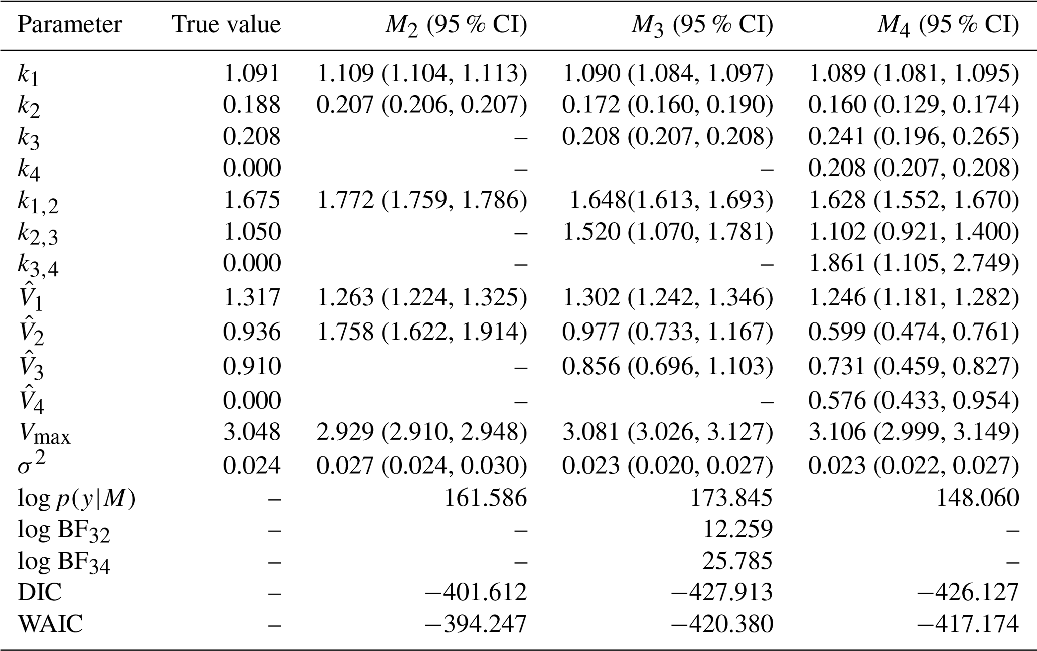
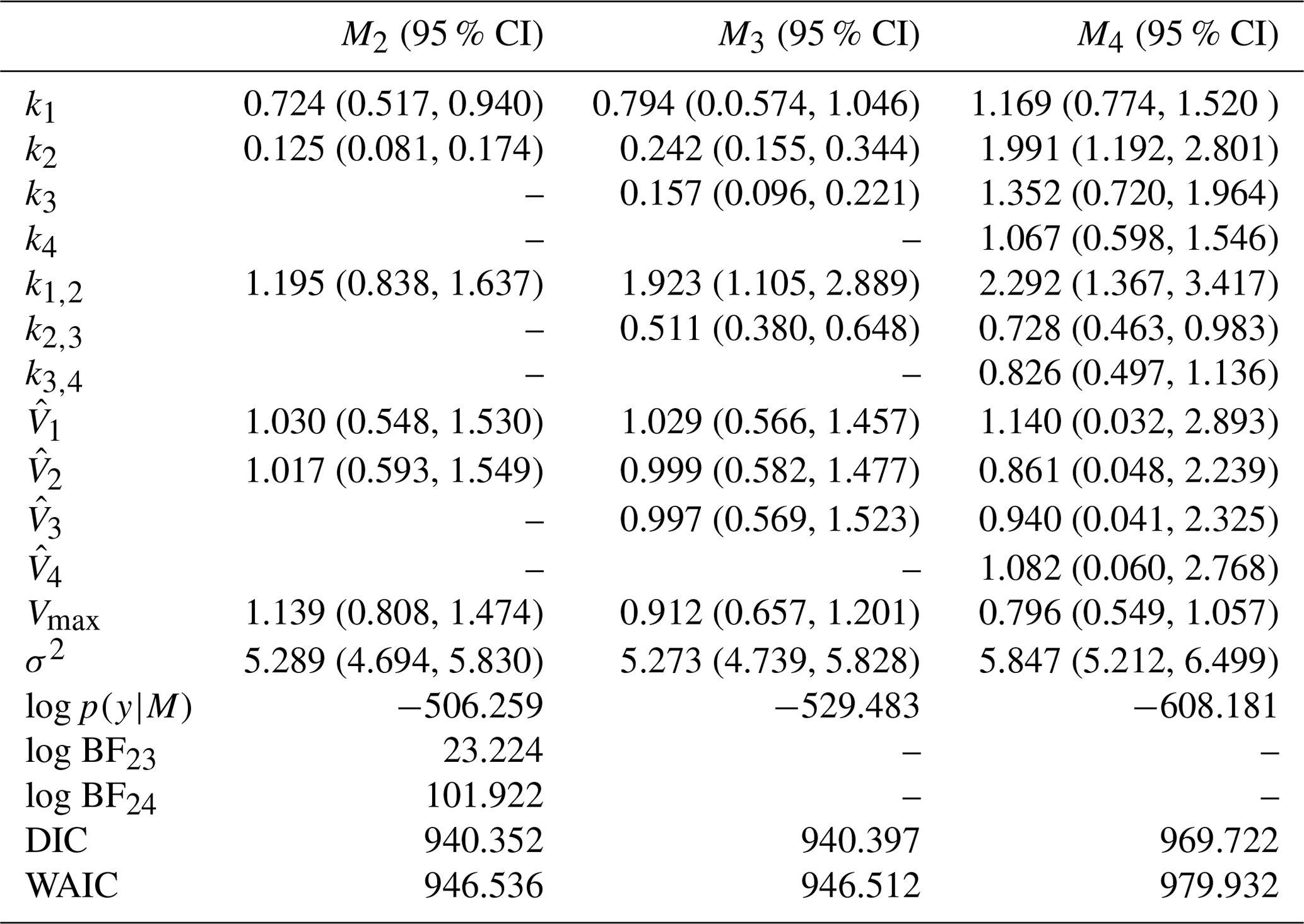
The posterior parameter estimates and 95 % credible interval (CI) are in Table 4. For M₂, the true model, the posterior parameters are very close to the true values and are within the 95 % CI. Moreover, the parameters k₁, ${\widehat{V}}_{\mathrm{1}}$, ${\widehat{V}}_{\mathrm{2}}$, V_max, and σ² are very close to the true values. However, the error term, σ², is the same for all three models as all models fit the data well. Therefore, a model selection criterion is needed to discriminate between models.

Fifteen marginal likelihoods are calculated in parallel for each model. The mean log marginal likelihood is presented in Table 4. We can calculate the log BF of any model compared to another by taking the difference in their log marginal likelihoods. Based on the interpretation of BF in Table 1, there is decisive evidence in favour of the data-generating model M₂.

The distributions of the log marginal likelihood for each model are shown in box plots (Fig. 7). In addition, the DIC and WAIC are shown along with those of the marginal likelihood, and they also select the data-generating model. The DIC is a Bayesian generalization of information-theory-based criterion AIC for model selection introduced by Spiegelhalter et al. (2002). The WAIC is based on pointwise out-of-sample predictive accuracy (Vehtari et al., 2017; Watanabe and Opper, 2010) and for large samples equivalent to the leave-one-out cross-validation (Watanabe and Opper, 2010). For these information-based theoretic methods, a difference of 10 is usually required for a decisive preference of one model over the other (Burnham and Anderson, 2002b, p. 70). A difference of up to 7 is considered less evidence for preferring one model over the other (Spiegelhalter et al., 2002). Model M₂ has the largest median log marginal likelihood, while model M₄ has the lowest.

The prior and posterior distributions for model M₂ are in Fig. 8. The prior distribution is in blue, while the posterior is in red. The prior range is wide compared to the posterior, so the posterior contours are too small. The posterior marginal densities are also more contracted compared to the prior densities, as seen on the diagonal of the plots. The prior contours show no significant correlation between the parameters.

The posterior distributions for this model are shown in Fig. 9. The marginal posterior distributions are on the diagonal. The red dots represent the true parameters. There is also a high correlation between pairs $(k_{\mathrm{1}},k_{\mathrm{2}}),(k_{\mathrm{1}},V_{\max }),(k_{\mathrm{1},\mathrm{2}},k_{\mathrm{2}}),(k_{\mathrm{1},\mathrm{2}},V_{\max }),(k_{\mathrm{2}},V_{\max })$, and $({\widehat{V}}_{\mathrm{1}},{\widehat{V}}_{\mathrm{2}})$.

Table 4 True value, posterior mean with 95 % credible intervals of the parameters and log marginal likelihood of the models for experiment 1. Model M₂ has the highest log marginal likelihood and is the true model. The DIC and WAIC are also shown.

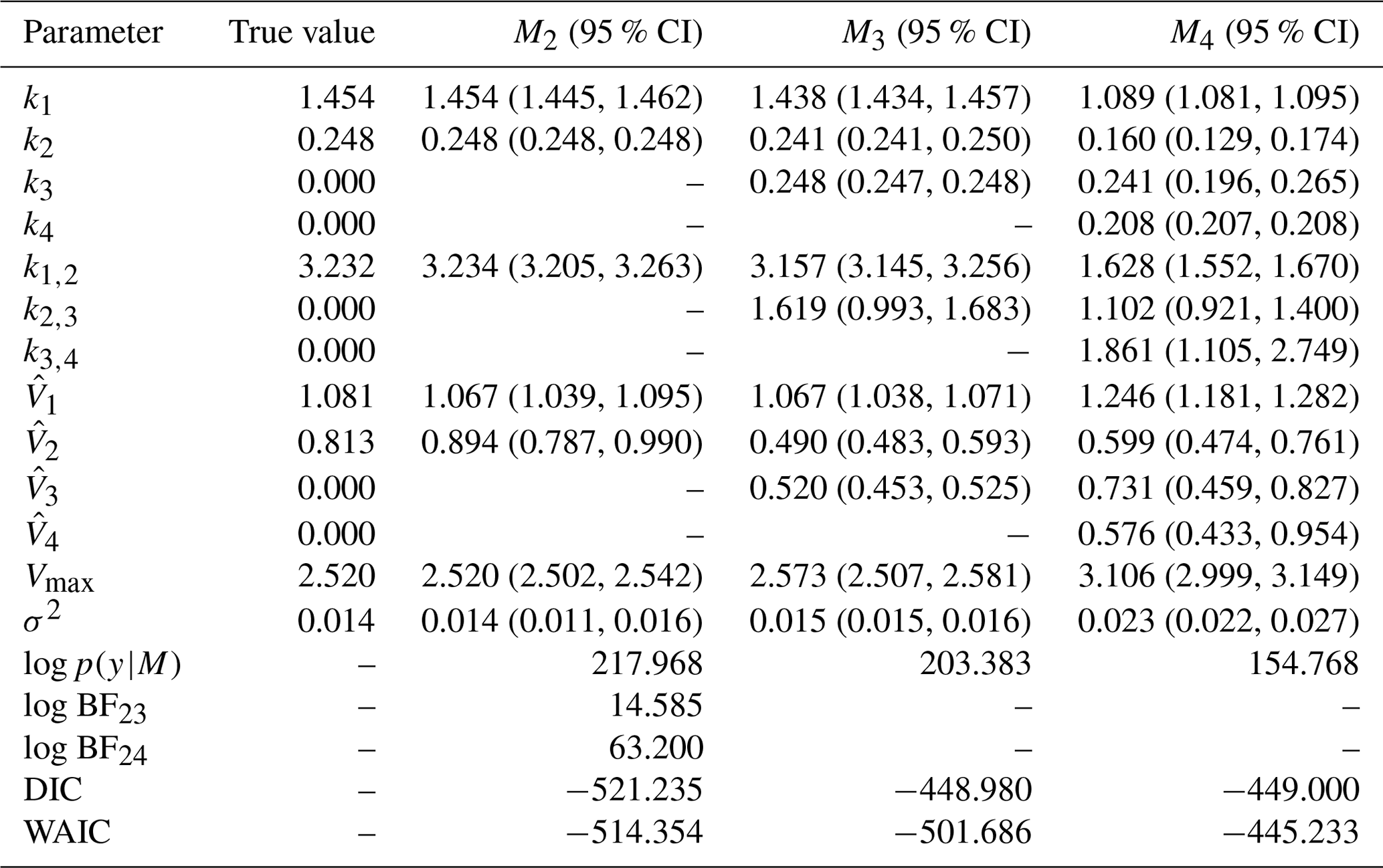
–: the parameter is not included in the model. σ²: error term. log p(y|M): log marginal likelihood. log BF_ij: Bayes' factor of model i compared to model j.

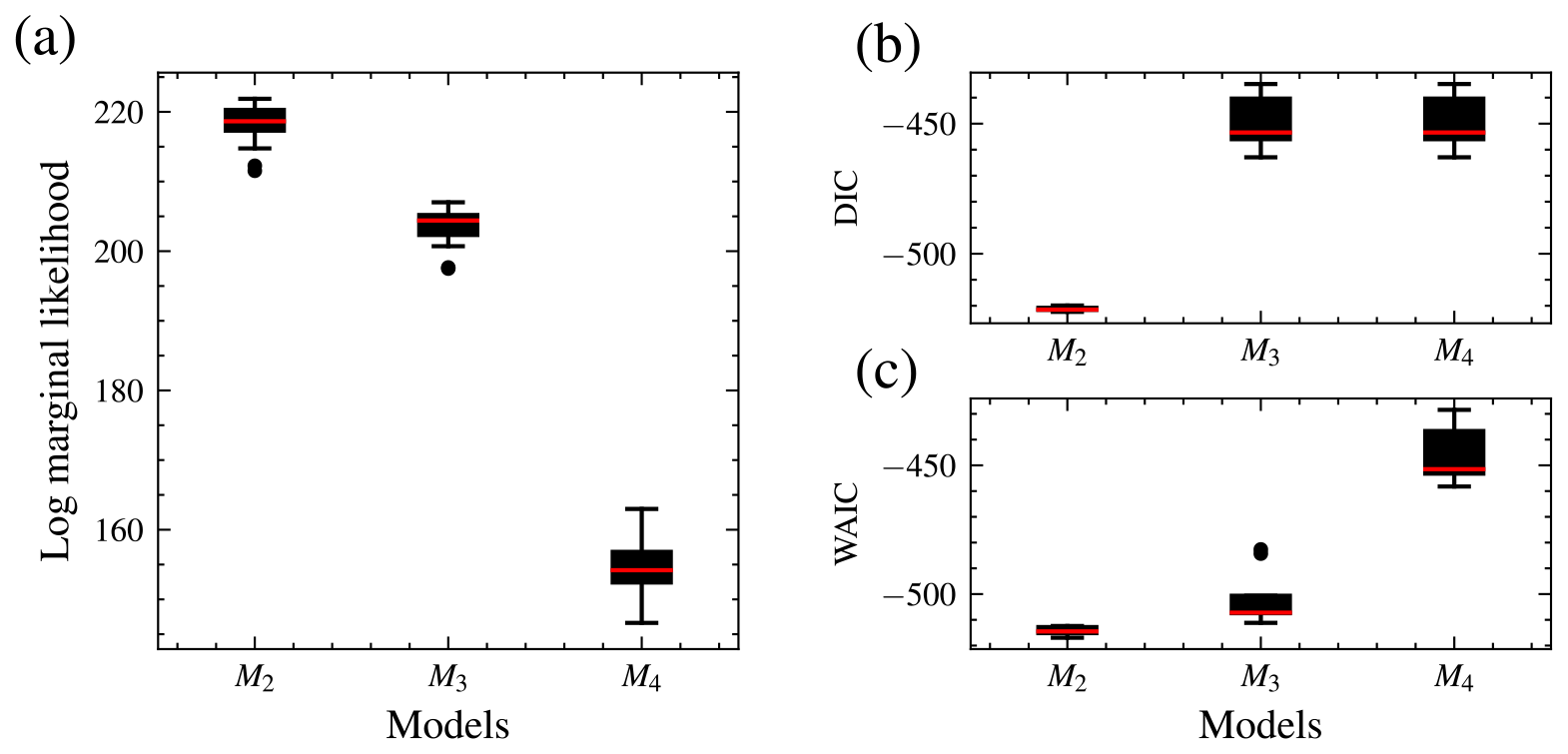
Figure 7 Distribution of the log marginal likelihood, DIC, and WAIC for 15 different runs each. Distribution of the log marginal likelihood for 15 different runs. The boxplot of the data-generating model, M₂, is the highest, while M₄ is the lowest. Hence, M₂ has the highest marginal likelihood. M₃ has the shortest interquartile range and, therefore, variability (a). DIC (b) and WAIC (c). For the log marginal likelihood, higher values are preferred, while for the deviance information criterion (DIC) and widely applicable information criterion (WAIC), smaller values are preferred. All techniques select the data-generating model.

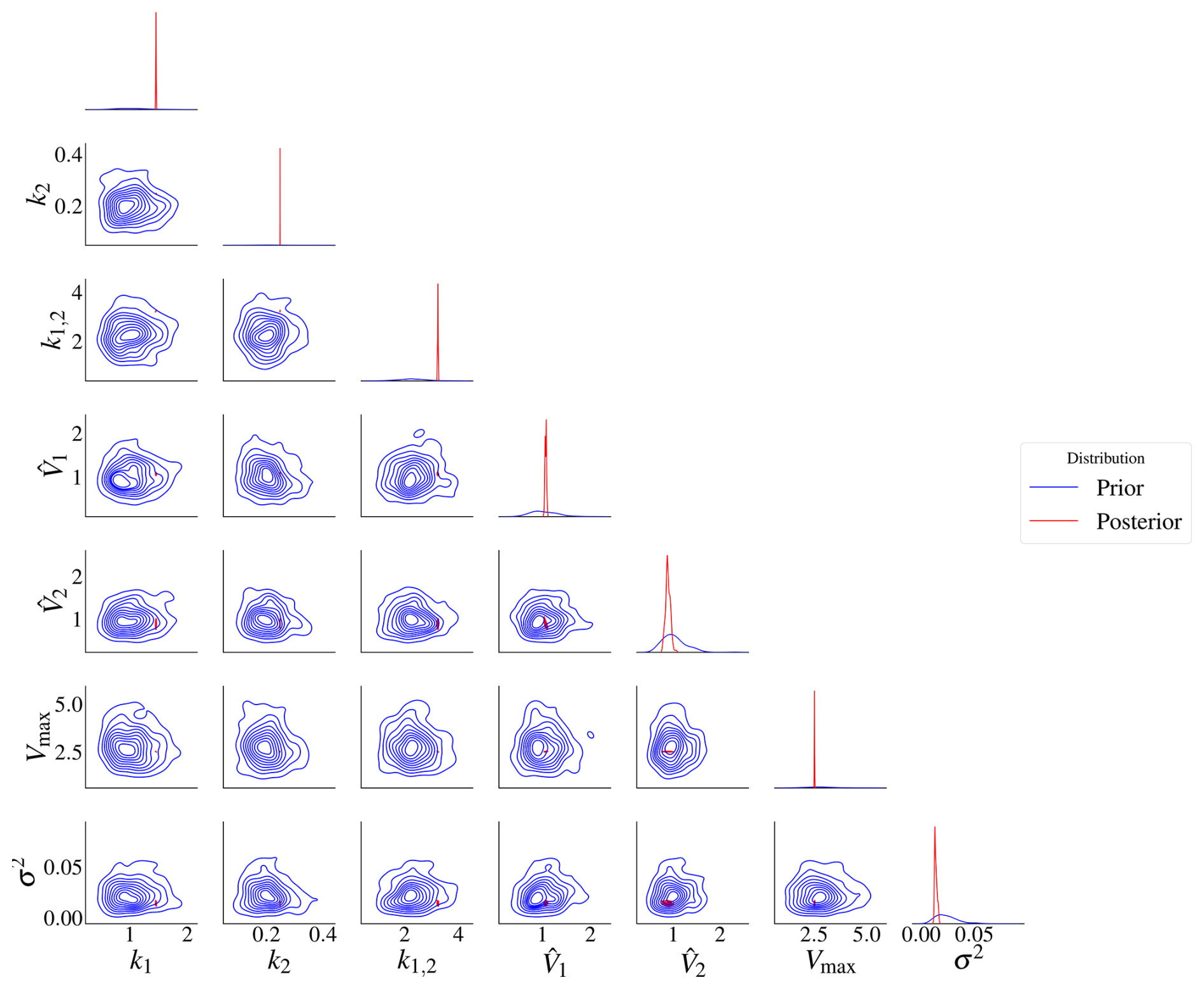
Figure 8 Prior and posterior distributions for model M₂. It is difficult to see the correlations due to the high difference in variance between the prior and posterior distributions. The red represents the posterior distributions and the blue the prior distributions. The posterior distributions have contracted compared to the priors.

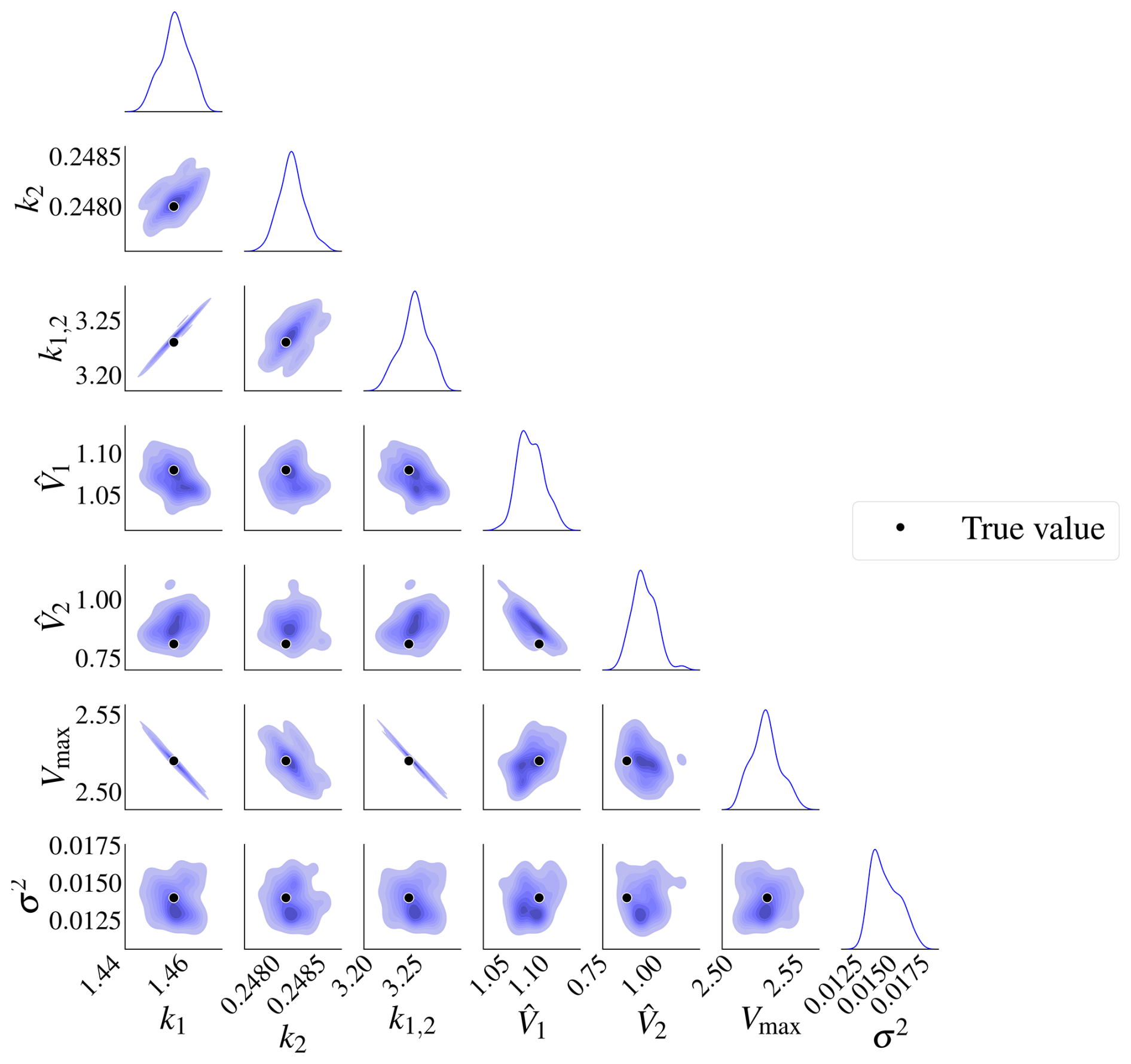
Figure 9 Posterior distributions for model M₂. There is a high correlation between k₁ and V_max, k_1,2 and k₂, and k_1,2 and V_max. The marginal posterior distributions are on the diagonal. The black dots represent the true parameters used in the data-generating process.

We also performed graphical posterior predictive checks. Discharge data were generated from the posterior predictive distribution of each model and plotted. There is no noticeable visual difference in discharge (Fig. 10) for all the models since the posterior error estimate is too small for all models. We also calculated PPP for the selected model using autocorrelation as a discrepancy measure. Hence, Eq. (8) becomes

$$\begin{array}{}\text{(20)}& \mathrm{ppp}\left(y_{\mathrm{obs}}\right)={\displaystyle \frac{\mathrm{1}}{n}}\sum _{i=\mathrm{1}}^{n}I\left[\right({\mathit{\rho }}_i^{\mathrm{rep}},{\mathit{\theta }}_i)\ge ({\mathit{\rho }}_{\mathrm{obs}},{\mathit{\theta }}_i\left)\right].\end{array}$$

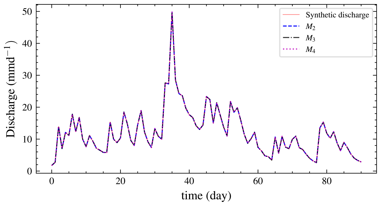
Figure 10 Plot of the mean discharge data generated from the posterior predictive distribution of each model for experiment 1. It is difficult to choose one model by inspection as they all fit the data well. However, the BF implicitly penalizes the unnecessarily complex models M₃ and M₄ and correctly selects M₂.

Posterior predictive plots might not tell us if the chosen model fits the data well, especially for dense datasets. Therefore, formal posterior predictive tests based on the discrepancy measure are needed. Like most statistical tests, the results will depend on the type of discrepancy measure or the test statistics. Carefully choosing such discrepancy measures is crucial. For example, we may test whether the model can predict peak discharge values, which would require a different discrepancy measure than if the aim of our analysis was to predict the mean values. Hence, we suggest using formal posterior predictive tests and graphical posterior predictive checks as in this study.

The PPP is 0.51, which means that the model has good predictive performance. This is expected for synthetic data. Values further from 0.50 indicate a model mismatch with the data. Values closer to 0 indicate that the model predictions are lower than the observed data. In contrast, values closer to 1 reveal that predictions are higher than observed data. A plot of the autocorrelations of predicted versus synthetic observed data is shown in Fig. 11. The proportion of values above the 45° line is the PPP. We also calculated PCPPP for the selected model and got a value of 0.64 > 0.05, which implies the model can generate the data. The PCPPP is calibrated based on prior predictive distribution and is uniformly distributed. Thus, it has the same interpretation as a classical p value.

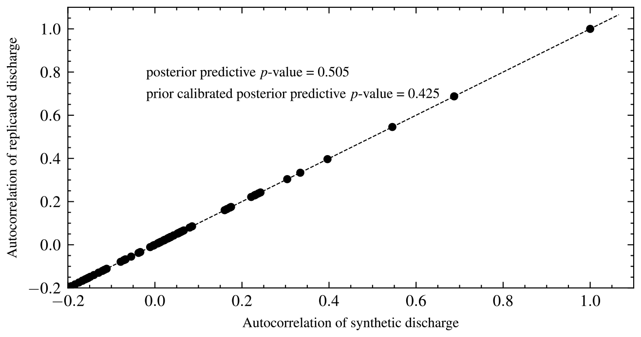
Figure 11 Autocorrelation of the replicated versus observed synthetic discharge data. The posterior predictive p value is the proportion of observations above the 45° line. The autocorrelation of the first point is 1, which isolates it from the other observations.

3.2.2 Experiment 2 with data generated from the three-bucket model, M₃

For the second experiment, the data model is M₃. Model M₃ has three more parameters than M₂ and three fewer parameters than model M₄. The priors for model M₂ and M₃ are shown in Table 3. The data in this experiment were also generated to follow the same trend as the observed data. All models were fitted to the data, and inference is based on 20 000 posterior samples with a burn-in of 5000. As explained above, convergence was checked using IAT and Geweke diagnostics. The posterior estimates are in Table 5. Although the error term is small for all models, M₂ has a higher value than the other two models, suggesting that it may not have the right complexity. Fifteen marginal likelihoods were also calculated for each model in parallel. The mean log marginal likelihood is presented in Fig. 5. The results are also shown in box plots in Fig. 12. The box plots reveal that M₃ has the highest median log marginal likelihood, and M₂ the lowest. There is decisive evidence in favour of model M₃, the expected result.

Following the recommendations in Burnham and Anderson (2002a) for interpreting information-theoretic criteria, a difference of 4 to 7 suggests a weak preference for a model, and a difference of at least 10 suggests strong preference for a model. Consequently, the DIC and the WAIC do not suggest a strong preference for the true model (M₃) over the richer model (M₄). The WAIC shows possible weak evidence in favour of M₃ over M₄, but we note that the error bar in Fig. 12 for WAIC M₄ indicates substantial uncertainty in the estimate. In this case, the BF then decisively selects the data-generating model M₃ where the information-theoretic criteria fail to do so. This example alone is clearly not proof that the BF is always superior to WAIC or DIC, but it suggests that there are cases in which BF succeeds and information-theoretic criteria can fail. The success of the BF of course comes with a significantly higher computational cost.

As in experiment 1, a hydrograph from the posterior predictive distribution is shown in Fig. 13. From the hydrograph, we cannot determine the best model through visual inspection since all the models fit the data equally well. Therefore, we require a formal model selection technique, such as the BF.

Table 5 True value, posterior mean with 95 % credible intervals of parameters, and log marginal likelihood of models for experiment 2. M₃ the true model has the highest log marginal likelihood. The DIC and WAIC are also included.

–: the parameter is not included in the model. σ²: error term. log p(y|M): log marginal likelihood. log BF_ij: Bayes' factor of model i compared to model j.

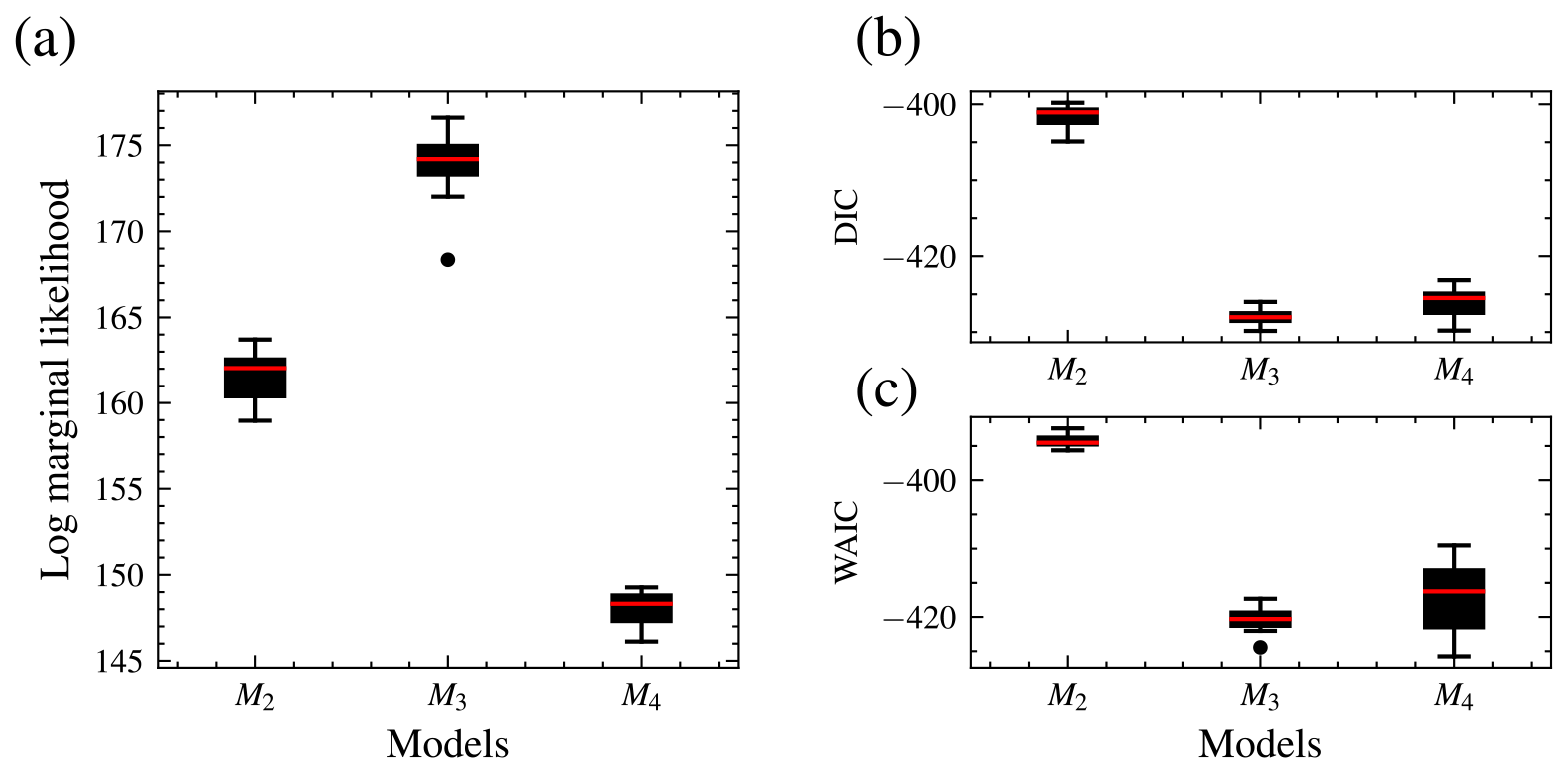
Figure 12 Distribution of the log marginal likelihood, DIC, and WAIC for 15 different runs, each with different initial parameter values. M₃, the data-generating model, has the highest median log marginal likelihood (a), while M₄ has the lowest. M₄ has the highest number of parameters, while M₂ has the fewest parameters. DIC (b) and WAIC (c). For the log marginal likelihood, higher values are preferred, while for the DIC and WAIC, smaller values are preferred. The log marginal likelihood selects the data-generating model, while DIC and WAIC do not have any preference for models M₃ and M₄.

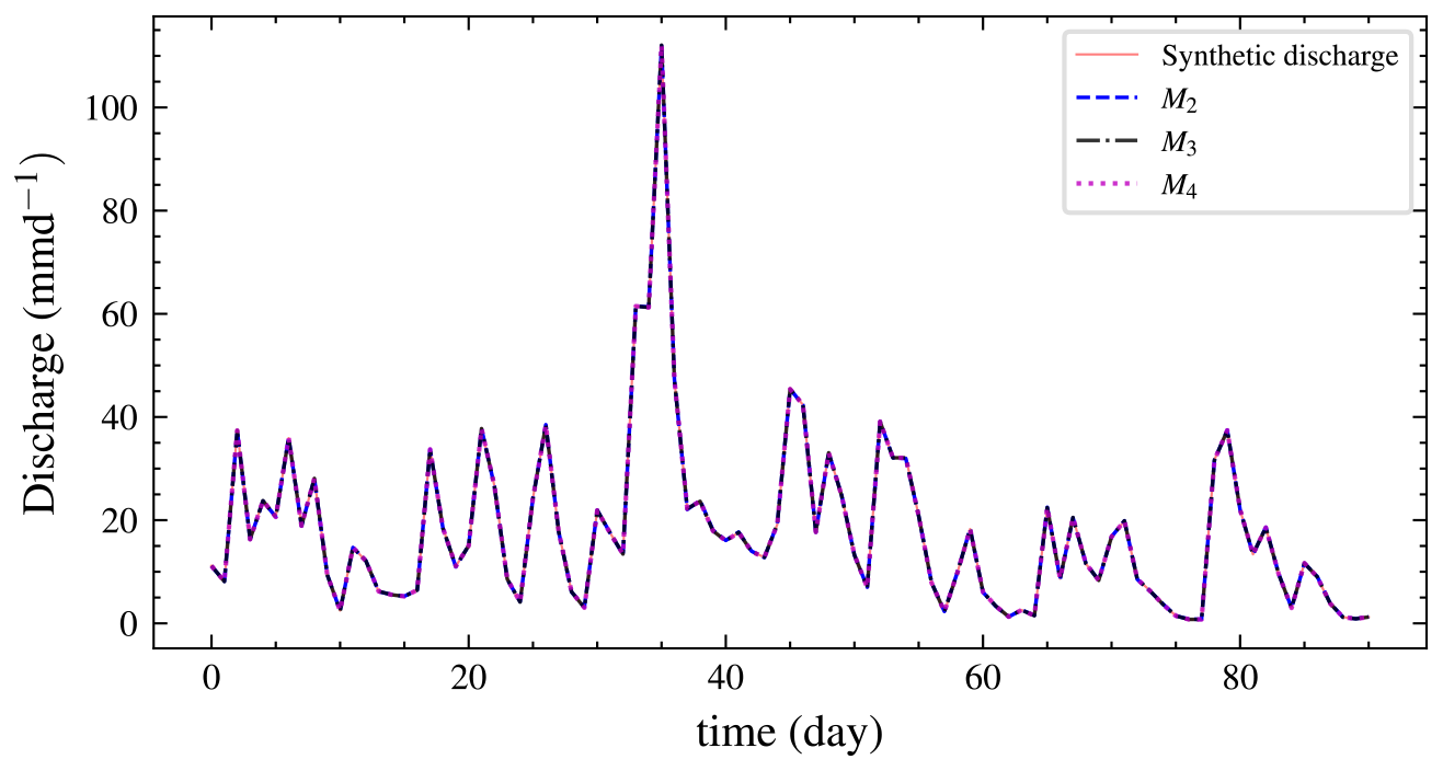
Figure 13 Plot of the mean discharge data generated from the posterior predictive distribution of each model for experiment 2. It is difficult to choose one model by inspection as they all fit the data equally. The BF implicitly penalizes the unnecessarily complex model M₄ and correctly selects M₃.

3.3 Real data experiment

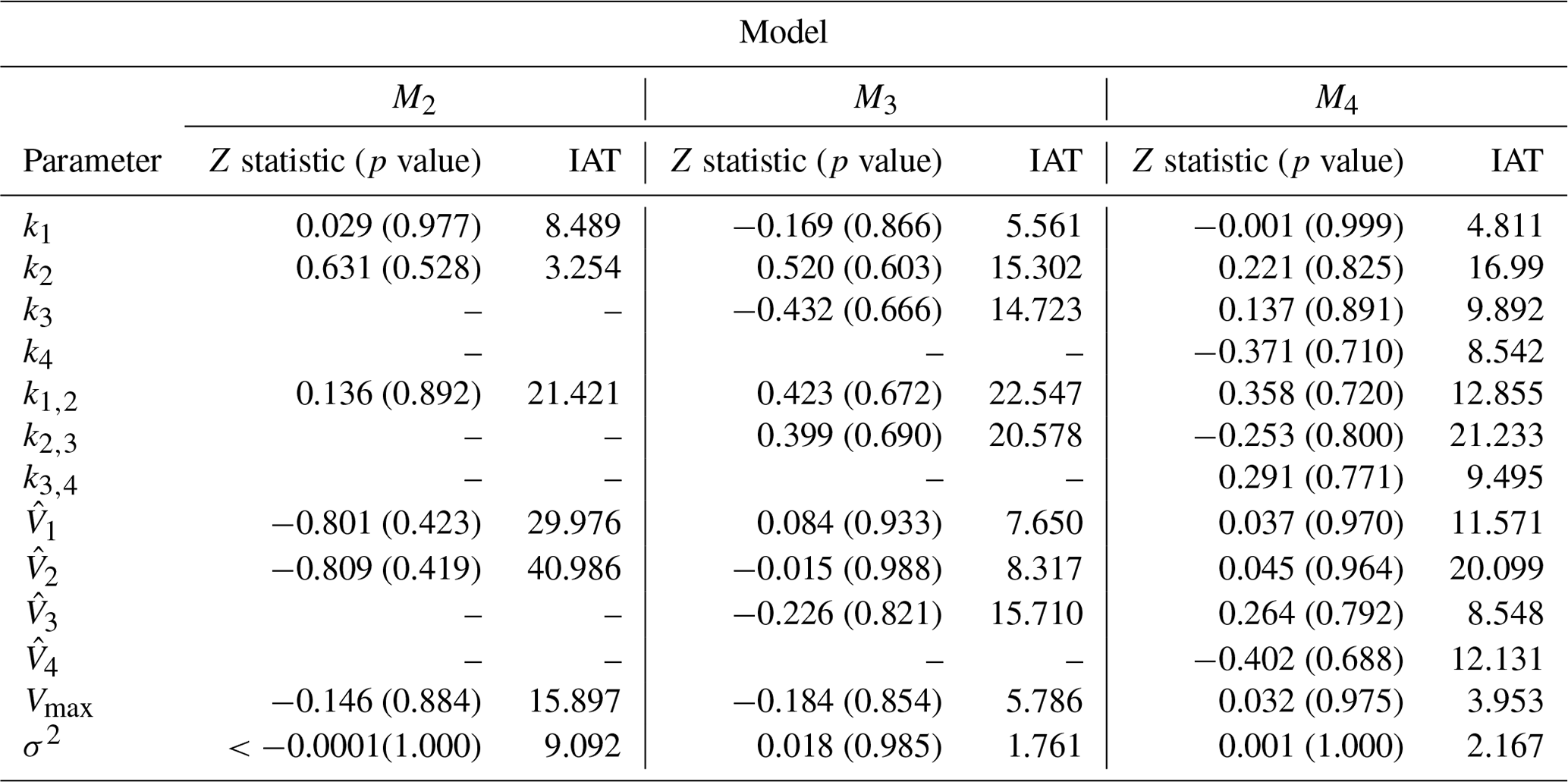
This section uses real-world discharge data for Magela Creek in Australia. For each model, 10 chains of the REpHMC were run as in the previous examples. We obtained 4000 posterior samples per chain, discarding the first 1000 as burn-in. The trace plots showed no indication of non-stationarity of the Markov chain, and both Geweke diagnostics and IAT supported convergence. The Z statistic, p value, and IAT are shown in Table 7. All p values are greater than 0.05, indicating no significant difference in the means of earlier and later posterior samples and no evidence against convergence. The null hypothesis states that the mean of the earlier and later posterior samples are equal. Furthermore, the IAT is less than $S/\mathrm{50}$ for all parameters, indicating well-mixed and stationary chains, where S represents the number of posterior samples. Smaller values of IAT indicate that fewer samples are needed to obtain an independent sample in the Markov chain.

Since we do not use an objective Bayesian approach, we used two sets of priors, where the second set is a sensitivity analysis. The first set of priors has higher variances for some parameters and is less informative than the second set (Table 6). It is common practice to try different priors and to check if the parameter estimates change with different priors. This is known as prior-sensitivity analysis. The models converge faster with the second set of priors. The first set of priors (Table 3) is the same as in the previous sections. For the second set of priors, we used lognormal priors with lower variances for some parameters compared to the first set of priors. The mean values used for the priors are also different from those of the first set of priors. The prior to the error term remains unchanged.

Table 6 Second set of priors. LN is the lognormal distribution, and IG is the inverse gamma distribution.

We checked the precision of our chosen model by comparing predicted and observed discharges using a posterior predictive check based on a second set of priors. The hydrographs for all three models are in Fig. 16. The plots of the predicted and observed autocorrelations with PPP are in Fig. 17. The PPP is 0.444, which is not too close to 0.5, and the PCPPP is 0.639. Hence, one can conclude that the model fits the data based on autocorrelation. Instead of autocorrelation, another metric could be used for the posterior predictive check depending on the objective of the model. The NSE for the chosen model is 0.526, and the KGE is 0.705. This means that the model performs better than using the mean observed discharge. Knoben et al. (2019) found that the KGE is $<-$0.41 when the model performs more poorly than the mean observed discharge. The marginal posterior distributions for model M₄ are shown in Fig. 14. We have also presented the posterior distributions of the parameters in model M₃ in Fig. 15. There is no noticeable correlation between parameters when real-world discharge data are used. However, V_max plays a major role in the dynamics of the model. A more realistic prior for V_max based on the soil physics of Magela Creek Australia will reduce the model error.

The results of the second set of priors are in Table 8. The selected model did not change when we used diffuse priors. The error in the second set of models is lower than in the first set. Model M₂ is always preferred, while M₄ is always the least supported one by the data. The error term, its precision, effective sample size (ESS), and the number of parameters influence the marginal likelihood.

We also applied two fully Bayesian information criteria, DIC and WAIC. Unlike the BF, there is no clear model choice for the information criteria. The difference in DIC or WAIC between M₂ and M₃ is less than 1, which means we do not have a reason to choose one model over the other.

RWM, NUTS, and MALA were also applied to all the three models with real world data. Even the other gradient-based algorithms, NUTS and MALA, could not sample the parameter space. Attempts to improve algorithms by trying various values for the initial step size in the case of NUTS and the step size for MALA did not make any difference. This further confirms the fact that combining replica exchange with an algorithm improves mixing and convergence.

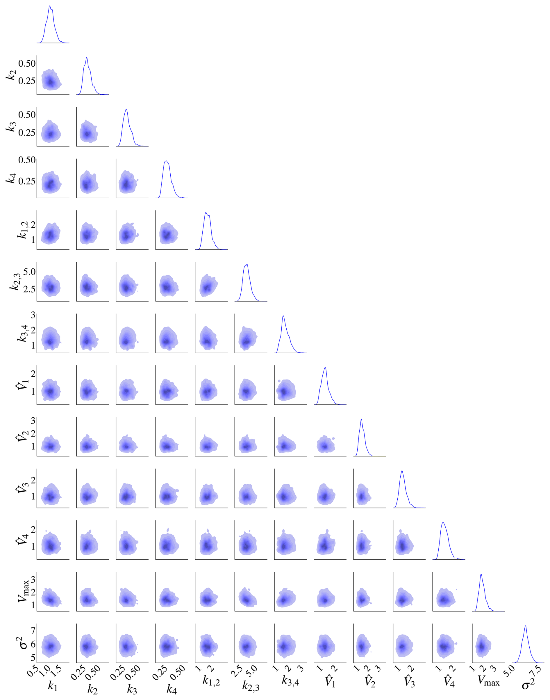
Figure 14 Posterior distributions of the 13 parameters for model M₄ using the second set of priors. There is no obvious correlation between the parameters. The marginal posterior distributions are on the diagonal.

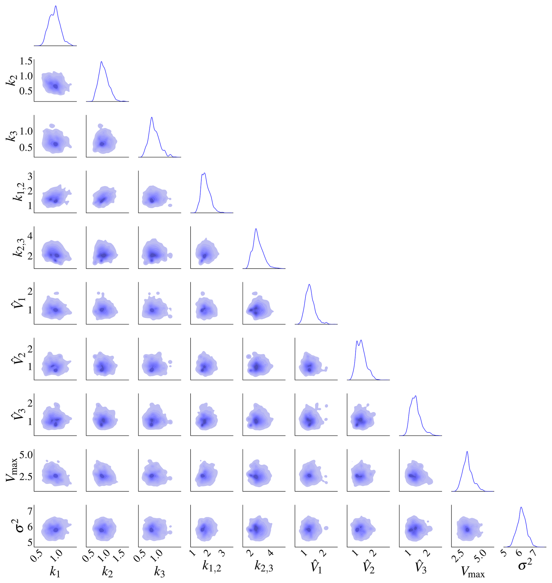
Figure 15 Posterior distributions of the 10 parameters of model M₃ based the second set of priors. There is no pronounced correlation between the parameters. The marginal posterior distributions are on the diagonal.

Table 7 Convergence diagnostics for real-world data: Z statistic, p value, and IAT. The null hypothesis is that the mean of earlier posterior samples is the same as that of later posterior samples in a Markov chain. All p values are above 0.05, indicating no significant difference in the mean of earlier and later posterior samples and no evidence against convergence. The IAT is the number of samples required to obtain an independent sample in the Markov chain, and smaller values are preferred.

3.3.1 Hydrograph of model M₂

Based on the hydrograph in Fig. 16, most of the model predictions are very close to the observed discharge and within 50 % pointwise credible intervals. However, two peaks are not captured in the model. The first peak discharge period was from 4 to 5 February 1980. The observed precipitation during this period is 41.4 to 122 mm d⁻¹ on 4 and 5 February 1980, respectively. The observed discharge on these days is 62.09 and 21.82 mm d⁻¹, respectively. It is illogical that the discharge is reduced with similar weather conditions. The second peak event occurred on 19 February 1980, with a precipitation of 15.70 mm d⁻¹ and discharge of 40.00 mm d⁻¹.

The precipitation on the previous day, 18 February 1980, was 39.30 mm d⁻¹ with potential evapotranspiration similar to other days and a lower discharge of 9.46 mm d⁻¹. This observed discharge is irrational as there is higher discharge with lower precipitation. Also, on 19 March 1980, the precipitation was 39.50 mm d⁻¹, with a discharge of 9.44 mm d⁻¹. In contrast, on 20 March 1980, the precipitation decreased to 28.30 mm d⁻¹, accompanied by an even lower discharge of 8.43 mm d⁻¹. This indicates a pattern of higher discharge with higher precipitation common on most days for similar weather conditions. An alternative explanation for the mismatch in peak discharge could be that the field capacity of the soil changed during these periods and is not captured in our models.

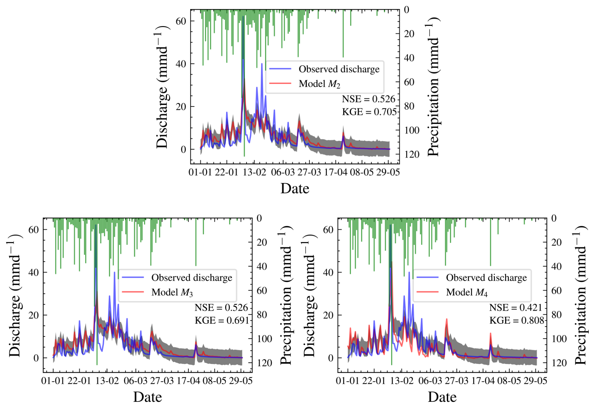
Figure 16 Hydrographs for all three models. Models M₂ and M₃ are not visually distinguishable. The results are better than the prior predictive check shown in Fig. 6, where most predictions are further from the observed data.

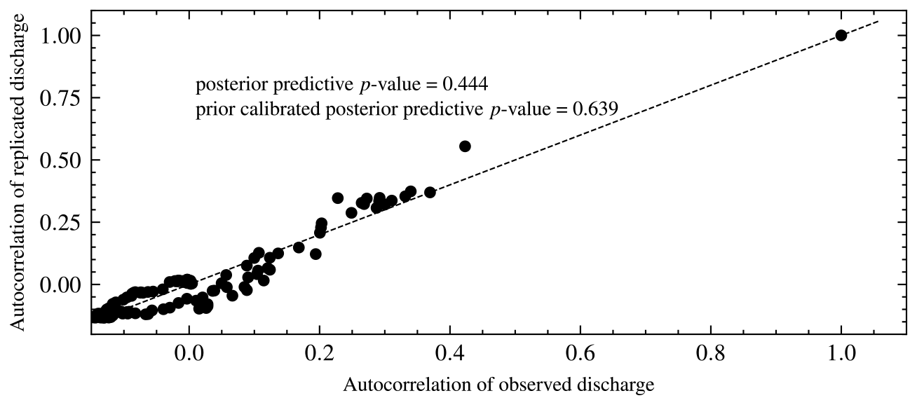
Figure 17 Autocorrelation of replicated versus observed data for model M₂. The posterior predictive p value is the proportion of observations above the 45° line.

Table 8 Posterior summary statistics and log marginal likelihood for models with the second set of priors. Model M₂ is the preferred over M₃ based on the log marginal likelihood. The difference in value between model M₂ and M₃ is less than 1 for both the DIC and the WAIC, so there is no preference between the two models according to these criteria. For information-theory-based approaches, a difference of 7 is necessary for a strong preference for one model. Model M₄ is the least preferred model based on any approach.

–: the parameter is not included in the model. σ²: error term. log p(y|M): log marginal likelihood. log BF_ij: Bayes' factor of model i compared to model j.

3.4 Convergence

3.4.1 Model convergence time

In terms of the theoretical complexity, if N is the number of posterior chains, S the number of samples per chain, and L the number of leapfrog steps per sample, then there are on the order of NSL likelihood and likelihood gradient evaluations for the algorithm to complete.

In terms of actual performance, all models converge by 3000 samples, even for real-world data. A single replica set runs on a single CPU core within a high-performance computer. The model runtime of Gaussian shell examples ranges from 6 s for 2 dimensions to 24 s for 30 dimensions. Synthetic examples converge in 2 to 4 h, depending on the parameter's dimension. On the contrary, with real data, the models converge in 6 to 20 h, depending on the parameter space and number of temperatures. Models can converge faster with proper tuning of the number of leapfrog steps. The posterior summary statistics, such as the mean of the parameters, do not change much with the number of temperatures. The number of temperatures mainly affects the estimate of the log marginal likelihood. With large datasets, REpHMC can be combined with subsampling without replacement to accelerate convergence. The REpHMC converges in minutes if we are interested only in parameter estimation.

3.4.2 Convergence of marginal likelihood

As proposed by Calderhead and Girolami (2009), most studies use 10 temperatures. However, it is important to check for convergence of the log marginal likelihood after convergence of the posteriors. We suggest starting from eight temperatures until the marginal likelihood is stable. That is the stopping point, when there is very little variation in the marginal likelihood. This can be visualized by a graph of the marginal likelihood against the number of temperatures. The number of temperatures at which the log marginal likelihood starts to plateau or flatten is the temperature at which it converges. Also, a horizontal line can be drawn at any point to see where most of the values lie or are close to the line, which helps to check for convergence. As observed with the Gaussian shell example, the marginal likelihood is constant from 10 to 12 temperatures. Thus, running beyond 12 temperatures is recommended. The diagnostic plot of the log marginal likelihood for the real-world example shows that it is constant from 10 to 12 temperatures too (Fig. 18). For the real-world data, we used 45 temperature schedules for each model. Also, The swap acceptance rate ranges from 0.169 for 10 temperature schedules to 0.379 for more than 44 temperatures.

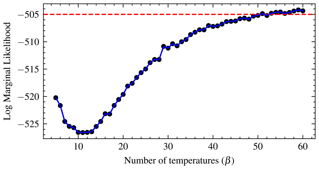
Figure 18 Convergence diagnostic of the log marginal likelihood for the two-bucket model. The optimal number of temperatures is 48 as there is a very small variation in the log marginal likelihood, and the curve begins to flatten. The values almost follow the red line from 45 temperatures.

4 Conclusions

We have introduced a methodology for simultaneous Bayesian parameter estimation and model selection. The methodology includes formal model diagnostics, which check for goodness of fit and prior data conflict. The method uses a new gradient-based algorithm REpHMC to draw posterior samples, TI for the calculation of marginal likelihood, and PCPPP for model diagnostics. The REpHMC and TI were validated on the Gaussian shell example, which is a difficult sampling benchmark problem since it has isolated modes. The REpHMC is effective in sampling the entire parameter space for models with isolated modes. This sets it apart from other gradient-based algorithms such as HMC, NUTS, and MALA. Also, we have shown that BF selects the data-generating model in two experiments, while DIC and WAIC correctly select the true model in one of two experiments. Also, none of the other mentioned gradient-based algorithms worked when real-world data were used with our developed model. In addition, formal posterior predictive checks have been introduced to determine if a model can accurately predict observed or desired values, such as the minimum or peak discharge. The method was employed to discharge data from Magela Creek in Australia. We also calculated NSE and KGE for the chosen model with real-world data. The framework has been implemented in open-source software TFP, which supports most algorithms. The REpHMC can be applied to any hydrological model. Our developed model performed better than using the mean as a predictor for real discharge data. However, the model does not capture peak discharge values. Therefore, some improvements in that regard need to be made.

By combining a gradient-based algorithm, HMC, and REMC, we obtain a powerful algorithm that can sample complex posteriors thanks to the exchange of information between parallel running chains. We have also illustrated that the BF is a reliable Bayesian tool for model selection in contrast to two common Bayesian-based information criteria for model selection.

Future work could combine REMC with the NUTS algorithm (Hoffman and Gelman, 2014) which requires less numerical parameter tuning than HMC. Also, introducing subsampling in the case of big data or models with millions of parameters will reduce the inference time. Another direction would be to focus on improving the model goodness of fit, as the KGE indicates. Furthermore, one could develop a discrepancy measure for the posterior predictive check to test whether the selected model can capture peak discharge values. On the practical side, this study could be extended to the multi-catchment setting. Also, different types of conceptual hydrological models could be compared using this approach.

Appendix A: Glossary

AIC	Akaike information criterion
BIC	Bayesian information criterion
HMC	Hamiltonian Monte Carlo
MALA	Metropolis-adjusted Langevin algorithm
pHMC	Preconditioned Hamiltonian Monte Carlo
REMC	Replica-exchange Monte Carlo
REpHMC	Replica-exchange preconditioned Hamiltonian Monte Carlo
REHMC	Replica-exchange Hamiltonian Monte Carlo
HBV	Hydrologiska Byråns Vattenbalansavdelning
NUTS	No-U-Turn Sampler
ODEs	Ordinary differential equations
ODE	Ordinary differential equation
TFP	TensorFlow probability
TF	TensorFlow
TI	Thermodynamic integration
MCMC	Markov chain Monte Carlo
IAT	Integrated autocorrelation time
BF	Bayes' factor
RWM	Random walk Metropolis
DREAM	Differential Evolution Adaptive Metropolis
PMC	Population Monte Carlo
CI	Credible interval
PPC	Posterior predictive check
PPP	Posterior predictive p value
PPL	Probabilistic programming language
PPLs	Probabilistic programming languages
PP	Probabilistic programming
PCPPP	Prior-calibrated posterior predictive p value
ESS	Effective sample size
NSE	Nash–Sutcliffe efficiency
KGE	Kling–Gupta efficiency
LN	Lognormal
IG	Inverse gamma
WAIC	Widely applicable information criterion
DIC	Deviance information criterion
ABC	Approximate Bayesian computation
ODEs	Ordinary differential equations