the Creative Commons Attribution 4.0 License.
the Creative Commons Attribution 4.0 License.
 | 24 Jul 2024
The Year of Polar Prediction site Model Intercomparison Project (YOPPsiteMIP) phase 1: project overview and Arctic winter forecast evaluation
Gunilla Svensson
Barbara Casati
Taneil Uttal
Siri-Jodha Khalsa
Eric Bazile
Elena Akish
Niramson Azouz
Lara Ferrighi
Helmut Frank
Michael Gallagher
Øystein Godøy
Leslie M. Hartten
Laura X. Huang
Jareth Holt
Massimo Di Stefano
Irene Suomi
Zen Mariani
Sara Morris
Ewan O'Connor
Roberta Pirazzini
Teresa Remes
Rostislav Fadeev
Amy Solomon
Johanna Tjernström
Mikhail Tolstykh
Although the quality of weather forecasts in the polar regions is improving, forecast skill there still lags behind lower latitudes. So far there have been relatively few efforts to evaluate processes in numerical weather prediction systems using in situ and remote sensing datasets from meteorological observatories in the terrestrial Arctic and Antarctic compared to the mid-latitudes. Progress has been limited both by the heterogeneous nature of observatory and forecast data and by limited availability of the parameters needed to perform process-oriented evaluation in multi-model forecast archives. The Year of Polar Prediction (YOPP) site Model Inter-comparison Project (YOPPsiteMIP) is addressing this gap by producing merged observatory data files (MODFs) and merged model data files (MMDFs), bringing together observations and forecast data at polar meteorological observatories in a format designed to facilitate process-oriented evaluation.
An evaluation of forecast performance was performed at seven Arctic sites, focussing on the first YOPP Special Observing Period in the Northern Hemisphere (NH-SOP1) in February and March 2018. It demonstrated that although the characteristics of forecast skill vary between the different sites and systems, an underestimation in boundary layer temperature variability across models, which goes hand in hand with an inability to capture cold extremes, is a common issue at several sites. It is found that many models tend to underestimate the sensitivity of the 2 m air temperature (T2m) and the surface skin temperature to variations in radiative forcing, and the reasons for this are discussed.
- Article
(17470 KB) - Full-text XML
- BibTeX
- EndNote


Recent decades have seen a marked increase in human activity in the polar regions leading to an increasing societal demand for weather and environmental forecasts (Emmerson and Lahn, 2012; Goessling et al., 2016). Despite this growing need, the skill of weather forecasts in the polar regions lags behind that of the mid-latitudes (Jung et al., 2016; Bauer et al., 2016). This is partly the result of the relatively low density of conventional observations at high latitudes compared to mid-latitudes (Lawrence et al., 2019) but is also related to the occurrence of meteorological situations and phenomena that are historically difficult to model, such as stable boundary layers (e.g. Atlaskin and Vihma, 2012; Sandu et al., 2013; Holtslag et al., 2013) and mixed-phase clouds (e.g. Pithan et al., 2014, 2016; Solomon et al., 2023), and the importance of coupling between the atmosphere and snow and ice surfaces (e.g. Day et al., 2020; Batrak and Müller, 2019; Svensson and Karlsson, 2011).
The ability of climate models to represent atmospheric processes in polar regions has recently been assessed highlighting deficiencies in near-surface and boundary layer properties (Pithan et al., 2014; Svensson and Karlsson, 2011; Karlsson and Svensson, 2013). Since many climate models are based on global weather forecasting systems, understanding the causes of forecast error after 1–2 d may help develop understanding of the sources of error in climate models (Rodwell and Palmer, 2007). Nevertheless, until recently there has been little focus on evaluating numerical weather prediction (NWP) models using in situ data from the terrestrial Arctic and Antarctic (Jung and Matsueda, 2016; Jung et al., 2016).
Recent studies, conducted as part of the World Weather Research Programme's Polar Prediction Project (PPP, Jung et al., 2016), have started to address this gap, assessing the skill of both the large-scale circulation (Bauer et al., 2016) and surface weather properties (Køltzow et al., 2019). The Year of Polar Prediction (YOPP) site Model Intercomparison Project (YOPPsiteMIP) was designed to build on these earlier studies by utilising process-level data from polar observatories to diagnose the causes of forecast error from a process perspective and ultimately inform model development. Although process-oriented evaluation studies focussing on polar processes are not new, those that have been done have tended to focus on one or two sites or a specific field campaign (see Day et al., 2020; Batrak and Müller, 2019; Miller et al., 2018; Tjernström et al., 2021; Kähnert et al., 2023, for some recent examples). A key aim of YOPPsiteMIP is to provide a pan-Polar perspective on forecast evaluation and process representation.
YOPPsiteMIP participants were asked to provide data in so-called merged data files (MDFs), which includes both merged observatory data files (MODFs), for observatory data, and merged model data files (MMDFs), for model data. These data standards, which were developed specifically for YOPPsiteMIP, are described by Uttal et al. (2024). Using this common file format, with consistent naming and metadata, facilitates equitable and efficient comparisons between models and observations. This standardisation of the data from different observatories also aids interoperability in the sense that the same evaluation code can be applied at different sites. These MDF filetypes were developed as part of PPP, following the FAIR (Findable, Accessible, Interoperable, Reusable) data principles (Wilkinson et al., 2016). Details of the MDF concept and specifics of the data processing chain for producing MDFs are described in Uttal et al. (2024).
The observatories selected for YOPPsiteMIP represent a geographically diverse set of locations (see Mariani et al., 2024). At these sites a wide range of instruments measuring properties of the air, snow and soil are employed, extending far beyond the traditional synoptic surface and upper-air observation network, which are collected for use in the production and evaluation of NWP systems (Uttal et al., 2015). Taken together, the observations collected at these observatories offer opportunities to develop a deeper understanding of the physical processes governing the weather in the polar regions, their representation in forecast models and how this varies from site to site. The processes and phenomena targeted in YOPPsiteMIP include boundary layer turbulence, surface exchange (including over snow and ice) and mixed-phase clouds.
A benefit of organising coordinated evaluation involving several NWP systems and multiple sites is that it helps clarify if the issues revealed by the analysis are model or location specific. The modelling community has organised model inter-comparisons to target various atmospheric processes relevant for Arctic conditions (e.g. Cuxart et al., 2006; Pithan et al., 2016; Tjernström et al., 2005; Sedlar et al., 2020; Solomon et al., 2023), with each using its own protocol for data sharing. However, the newly developed standardisation of the observational and forecast model data developed for YOPPsiteMIP is planned to be used for future MIIPs (Model Intercomparison and Improvement Projects). Converging on a standard like this will aid interoperability, making it easier for model developers to expand their evaluation to new sites or observational campaigns but also to other models or forecasting systems.
MDFs were requested for the locations listed in Table 1 and shown in Fig. 1 during the YOPP Special Observing Periods (SOPs), during which the observations taken at many polar observatories (e.g. the frequency of radiosondes) was enhanced (see Lawrence et al., 2019; Bromwich et al., 2020). For the Northern Hemisphere the periods February–March 2018 and July–September 2018 were selected and named NH-SOP1 and NH-SOP2, respectively. For the Southern Hemisphere or SH-SOP the period November–February 2018/2019 was chosen. At the time of publication MMDFs have been produced and archived from seven NWP systems for these periods, and all of the sites listed have MMDFs from at least one model. MODFs have been produced and archived for seven of the sites so far and it is hoped that additional MODFs will be produced in the future to fill the gaps, particularly in the Southern Hemisphere.
Table 1List of YOPPsiteMIP observatory locations: name, name as used in filenames (shown in italics), latitude, longitude and elevation. Where an elevation range is stated, this is because the instruments at a given observatory extend over a range of values due to variations in local topography.
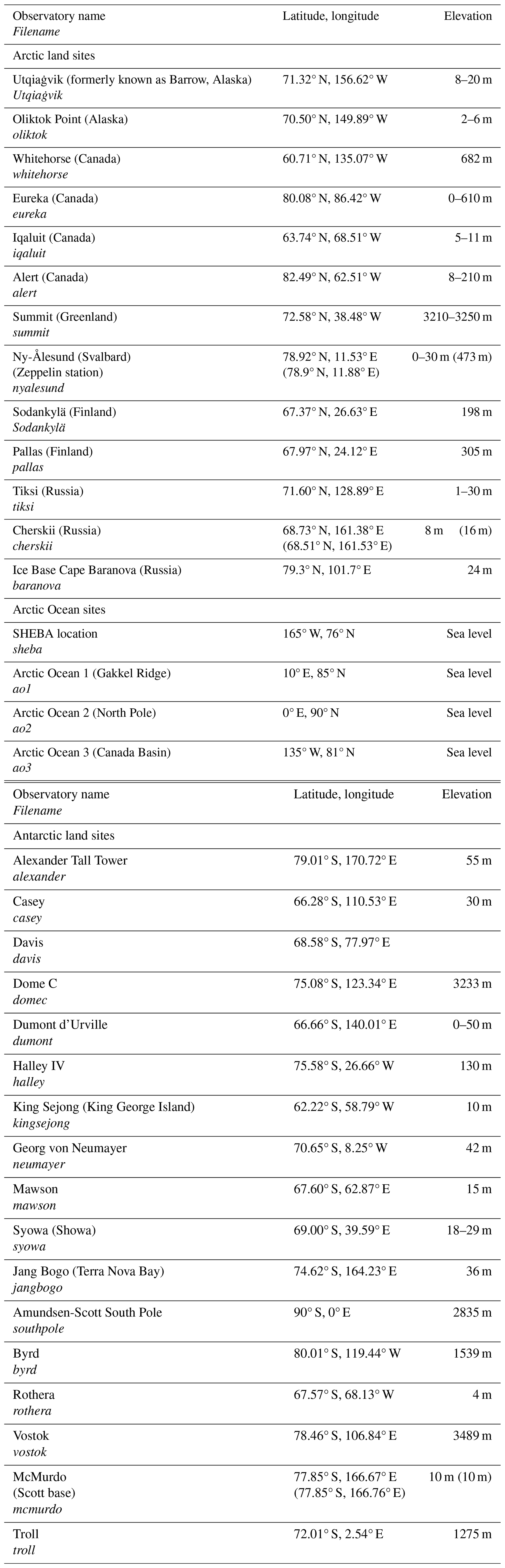
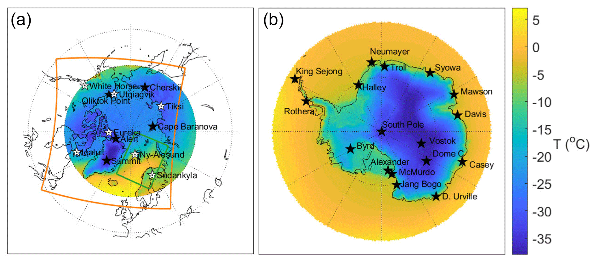
Figure 1Maps of the ERA5 2 m temperature climatology (1990–2019) for February–March (time of NH-SOP1) for the Arctic (a) and for November–February (SH-SOP) for the Antarctic (b). The observatories used in YOPPsiteMIP are marked with stars. White stars indicate the sites where MODFs are currently available, which are the subject of this study; black stars indicate the sites whose MODFs are not yet complete. The orange and green boxes depict the extent of the ECCC-CAPS and AROME-Arctic domains, respectively.
The purpose of this paper is twofold. First, it seeks to document the first version of the YOPPsiteMIP dataset along with a basic description of the forecasting systems and their respective MMDFs that are archived at the YOPP Data Portal, hosted by the Norwegian Meteorological Institute (MET Norway). Second, the paper presents a multi-site evaluation of seven forecasting systems during NH-SOP1 at seven Arctic observatories that have produced MODFs. The locations are indicated by the white stars in Fig. 1a, and the MODFs and full details of the sites are described in Mariani et al. (2024).
The seven Arctic sites used for evaluation in this study cover both high Arctic and sub-Arctic climate zones. Tiksi, Utqiaġvik, Iqaluit, Ny-Ålesund and Eureka all sit in the Arctic tundra characterised by low vegetation. The remaining two sites Whitehorse and Sodankylä are sub-Arctic, with higher vegetation corresponding to the boreal cordillera and taiga ecozones, respectively. Whitehorse, Iqaluit, Ny-Ålesund and Eureka are characterised by complex topography in the surrounding area, whereas the other sites are flatter. All the sites are in close vicinity to either frozen ocean (sea ice) or frozen inland waterbodies at this time of year, and the land surrounding each observatory is covered in snow throughout the period February–March 2018. A visual representation of the model grids with respect to the landscape surrounding these stations can be seen in Fig. 2 of Mariani et al. (2024) in which a more detailed description of the site characteristics may be found.
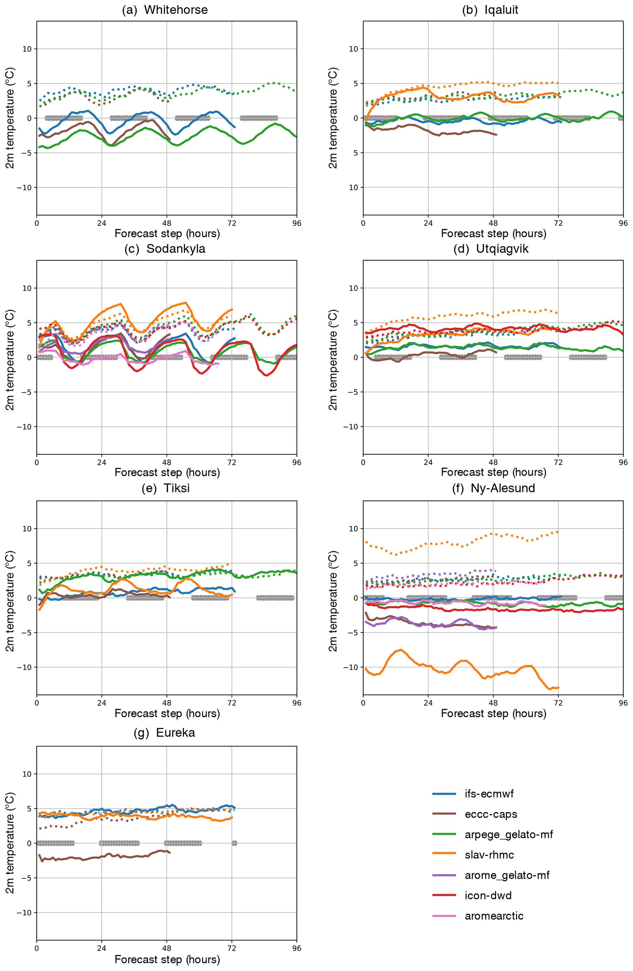
Figure 2Mean bias (solid lines) and standard deviation (dashed lines) of the 2 m temperature error (in °C) at each observatory (see Fig. 1a) for forecasts initialised at 00:00 Z during NH-SOP1, described in Table 2. Night-time periods (with mean SW↓ < 15 W m−2) are indicated with grey crosses along the x axis.
To date, six NWP centres have submitted forecasts from seven forecasting systems for NH-SOP1 and NH-SOP2, with two systems submitted for the SH-SOP (see Table 2). The following four systems are global:
-
the Integrated Forecasting System from the European Centre for Medium-Range Weather Forecasts (ECMWF-IFS; Day, 2023);
-
the Action de Recherche Petite Echelle Grande Echelle from Météo-France (ARPEGE-MF; Bazile and Azouz, 2023a);
-
the Semi-Lagrangian, based on the absolute vorticity equation from the Hydrometeorological Research Centre of Russia (SLAV-RHMC, Tolstykh, 2023);
-
the Icosahedral Nonhydrostatic Model from Deutscher Wetterdienst (DWD-ICON; Frank, 2023).
The following three systems are regional:
-
the Canadian Arctic Prediction System from Environment and Climate Change Canada (ECCC-CAPS; Casati, 2023)
-
and two versions of the Applications of Research to Operations at Mesoscale (AROME) from Météo-France (AROME-MF; Bazile and Azouz, 2023b) and from MET Norway (AROME-Arctic; Remes, 2023).
The domain boundaries of the regional forecasting systems can be seen in Fig. 1 (note that only two of the observatories are within the AROME domain). The forecasts analysed here were initialised at 00:00 UTC for each day of the SOPs (although 12:00 UTC forecasts are also available on the archive for many of the systems). The forecast lead time varies between the different systems but all forecasts are at least 2 d long (see Table 2 and Figs. 2 and 3).
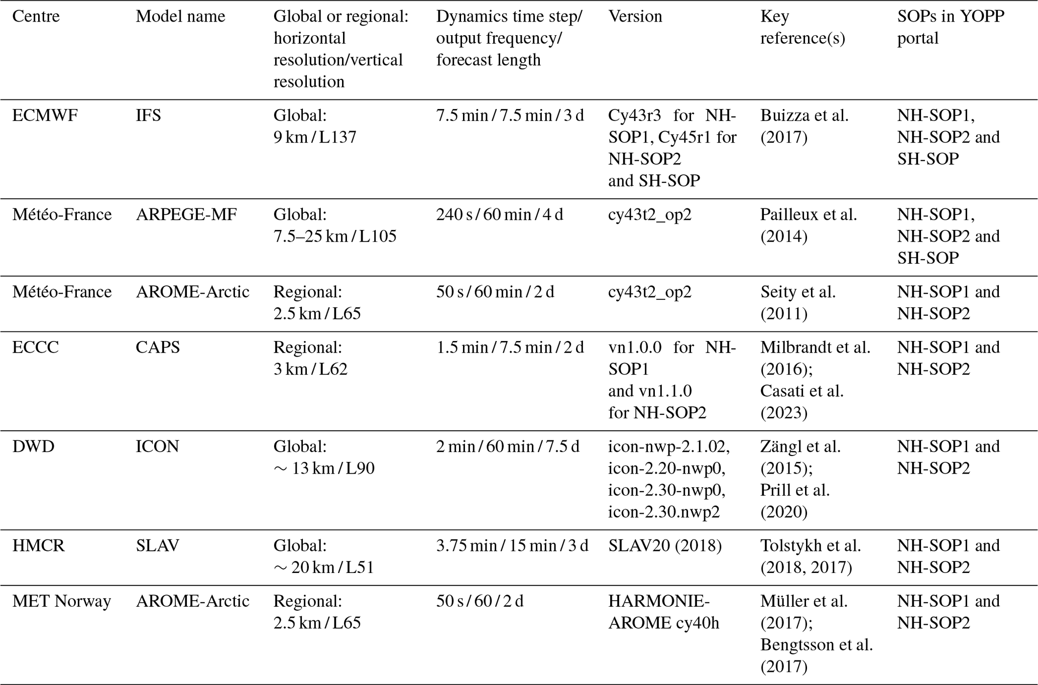
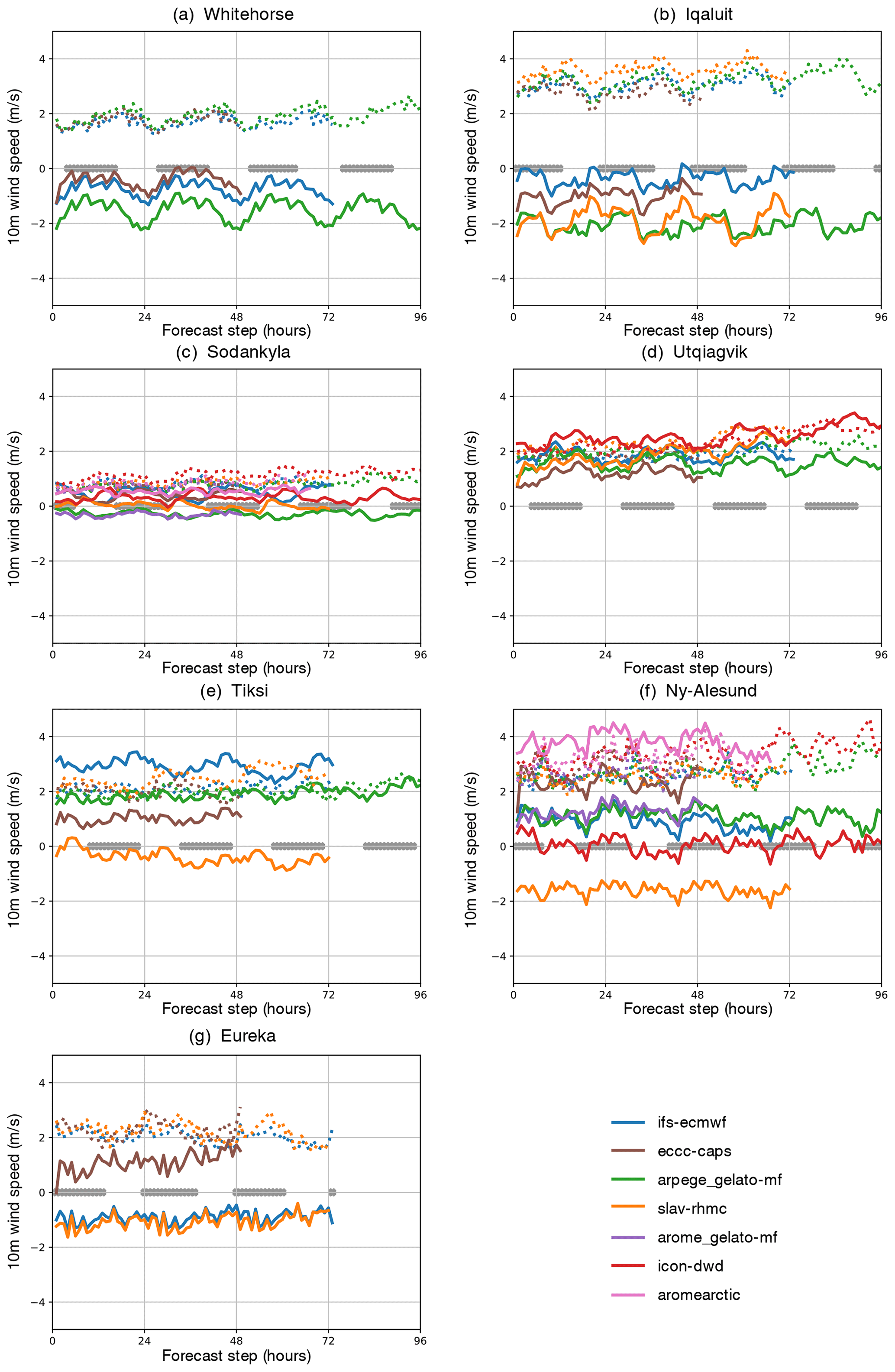
Figure 3Mean bias (solid lines) and standard deviation (dashed lines) of the 10 m wind speed error (in m s−1) at each observatory for forecasts initialised at 00z during NH-SOP1. Night-time periods (with mean SW↓ < 15 W m−2) are indicated with grey crosses along the x axis.
The files for some of the systems (CAPS, SLAV, ARPEGE, AROME-MF) are provided with multiple grid points centred on the observatory location. For others only a single grid point was provided. Multiple grid points centred around the observatory location were requested because many of the observatories are located in the vicinity of coasts, which leads to representativeness issues when comparing the land-based observation to model output for grid points being partially or entirely over the ocean. In this study, when there are multiple grid points we choose the closest 100 % land point to the supersite location, with the exception of CAPS, for which the central grid point within a beam of 7×7 grid points was considered (since nearest to the observation site) and ICON which provided the single closest grid point to the station location. As a result, the evaluation utilises a 100 % land grid box at all models and locations, with the exception of ICON, which has 23 % land cover at the Utqiaġvik and 73 % at Ny-Ålesund, and CAPS, which has 37 % land cover in Utqiaġvik; 71 % and 77 % in Tiksi and Iqaluit, respectively; and over 90 % land cover for the other sites. Comparison of the CAPS grid points surrounding Utqiaġvik with each other indicated that the evaluation would not be much influenced by the choice of grid cell (not shown) since during the Arctic winter the frozen ocean grid points have similar properties to the snow-covered land surface (e.g. when analysing the surface energy budget sensitivity to radiative forcing in Sect. 3.4). The grid resolutions range from 2.5 to ∼30 km, and the model time step varies from 1.5 to 7.5 min (see Table 2).
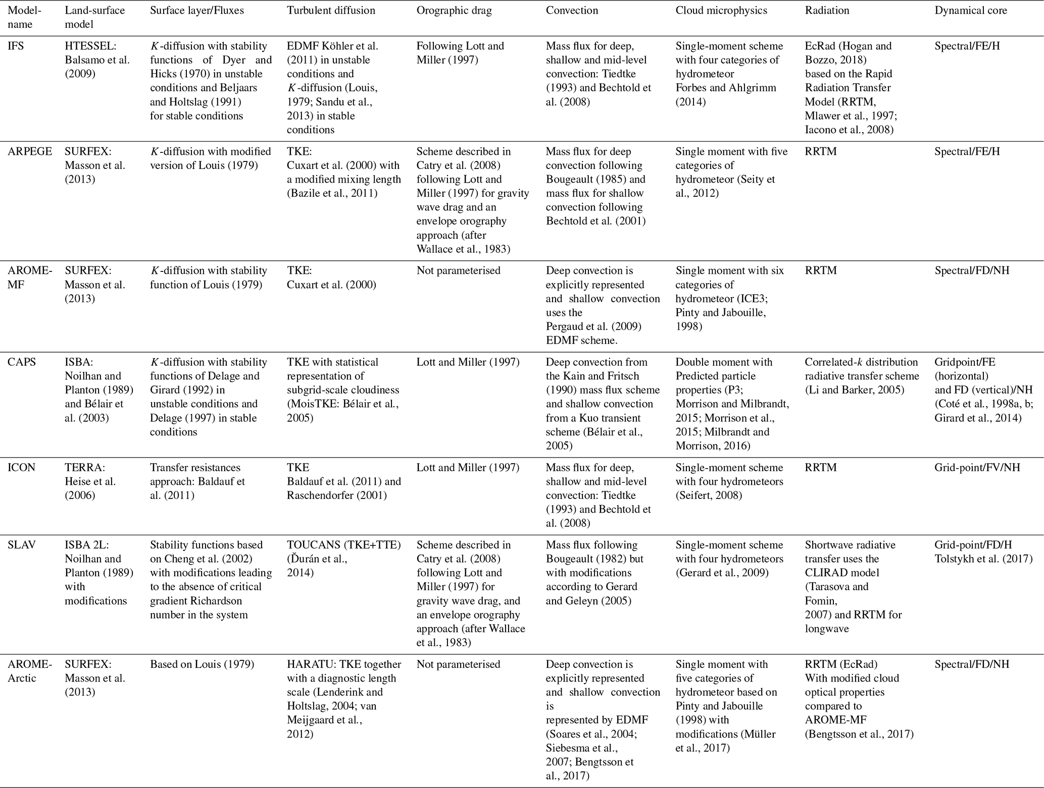
The models have quite a diverse mixture of formulations for atmospheric dynamics, land surface, sub-grid-scale parameterisations, and initialisation and data assimilation procedures. More details about the simulations with specific models are provided below and a summary of the key model components and parameterisations used in each model is included in Table 3.
Table 3Details of physical processes and parameterisations of the forecasting systems (see Appendix A for list of acronyms). Note that slashes are used in the right-hand column to separate information on the dynamical core of each model: model grid type/numerics/hydrostatic assumption.
2.1 IFS-ECMWF
MMDFs for the operational forecasts with the IFS high-resolution deterministic forecasts are available for the period starting January 2018. The initial forecasts are produced with IFS cycle 43r3, which was an atmosphere-only model with persistent sea ice and anomaly sea surface temperatures (SSTs). From 5 June 2018 (i.e. before NH-SOP2), the forecasts were produced with cycle 45r1, which included dynamic sea ice and ocean fields (see Day et al., 2022, for more information). Although the model version changes, the horizontal (∼9 km) and vertical resolution (L137) are the same in all SOPs. The data archived in the MMDFs is provided at the model time step (7.5 min) for a single model grid point closest to the observatory. In addition to the grid point data, a number of parameters (including albedo, surface temperature, and surface energy fluxes) are provided on the land surface model tiles to enable detailed evaluation of processes even at heterogeneous sites. A complete description for the two versions of the IFS can be found at the following link: https://www.ecmwf.int/en/publications/ifs-documentation (last access: 10 July 2024).
2.2 ARPEGE-MF
The version of ARPEGE submitted to YOPPsiteMIP was a pre-operational version based on the cy43t2_op1 operational system but coupled with the 1D sea ice model GELATO (Bazile et al., 2020). The resolution of the model used for these simulations is the same as is used operationally at Météo-France, which is variable (using a stretching factor of 2.2) with the pole (highest resolution of 7.5 km) over France for NH-SOP1 and NH-SOP2 and over Antarctica in SH-SOP and 105 vertical levels. The horizontal resolution is about 8–9 km over the North Pole, and time series have been provided for the three SOPs in the MMDF format for the 21 YOPP observatories with an hourly output for both state variables (instantaneous) and fluxes (accumulated).
2.3 SLAV-HMRC
MMDFs were produced by the SLAV model (Tolstykh et al., 2018) for both NH-SOP1 and NH-SOP2 containing 7 d forecasts starting at 00:00 UTC. The output is available for four horizontal grid points surrounding selected observatories every 15 min (i.e. every fourth time step). Depending on variable, the output is instantaneous or a 15 min averaged value. Data for 13 of the Arctic observatories in Table 1 are provided. The selection of observatories is based on model resolution in latitude, which is relatively low, i.e. ∼16 km in northern polar areas; in addition, the ao2 point is not included because the model grid does not contain the poles.
2.4 ICON-DWD
MMDFs from DWD's ICON (Zängl et al., 2015) are available from February 2018 to June 2020 containing 7.5 d forecasts starting at 00:00 and 12:00 UTC for Sodankylä, Ny-Ålesund and Utqiaġvik (Barrow). The mesh width is 13 km. Different model versions are used during this period. In February icon-nwp-2.1.02 was used followed by icon-2.3.0-nwp0 during 14 February 2018 to 6 June 2018, and from 19 September 2018 to 5 December 2018 icon-2.3.0-nwp2 was in operation. Since 14 February 2018, a new orographic dataset came into operation; however, for the three data points provided the changes were less than 1 m in height. The sea ice analysis used in ICON was based on the Real-Time Global SST high-resolution analysis of NCEP until 16 July 2018. Since then it has been based on the Operational Sea Surface Temperature and Sea Ice Analysis (OSTIA; Donlon et al., 2012) product. To represent variations in subgrid-scale surface characteristics ICON uses a tile approach. Since 16 July 2018 the tile values of surface fluxes and other tile-dependent variables are included in the MMDFs in addition to the grid average values. Hourly output is available based on a time step of 120 s.
2.5 CAPS-ECCC
MMDFs for ECCC-CAPS are available for the whole period from February 2018 to December 2018. Prior to 28 June 2018 CAPS was uncoupled and run with the GEM version 4.9.2. After 29 June 2018 CAPS was coupled with the Regional Ice and Ocean Prediction system (RIOPS) and run with the GEM version 4.9.4. Atmospheric lateral boundary conditions (LBCs) and initial conditions (ICs) are from ECCC Global Deterministic Prediction System (GDPS). Initial surface fields are from the Canadian Land Data Assimilation System (CaLDAS). The CAPS time series are produced for a beam of 7×7 grid points centred on each of the 12 land-based Arctic observatories listed in Table 1. Time series up to 48 h lead time are made available for the daily runs initialised at 00:00 UTC. The data are archived with a time frequency of 7.5 min, equivalent to five time steps of 90 s each.
2.6 AROME-ARCTIC
MET Norway utilises the HARMONIE-AROME (HIRLAM–ALADIN Research on Mesoscale Operational NWP in Euromed–Application of Research to Operations at Mesoscale) model configuration (Bengtsson et al., 2017) for operational weather forecasting for the European Arctic with the name AROME-Arctic (Muller et al., 2017). AROME-Arctic MMDFs are based on the operational forecasts (cy40h.1) and are available for the NH-SOP1 and NH-SOP2 at Sodankylä and Ny-Ålesund. LBCs are derived from the ECMWF IFS-HRES described in Sect. 2.1. Assimilation of conventional and satellite observation with 3DVAR in the upper atmosphere, optimal interpolation of snow depth, screen-level temperature and relative humidity in the surface model. Temperature tolerance in the surface assimilation scheme was increased on 15 March 2018 to better assimilate observed low temperatures. The data archived in the MMDFs are provided hourly for the single model grid point closest to the site. Model data for the full domain in its original format are also available via https://thredds.met.no (last access: 11 July 2024).
2.7 AROME-MF
The AROME-MF system from Météo-France and AROME-ARCTIC from MET Norway are both configurations of the same model system but use different parameterisations of turbulence, shallow convection, cloud microphysics, and sea ice. The system used for the YOPPsiteMIP differs from the operational AROME-France configuration (Seity et al., 2011) and the version evaluated for NH-SOP1 in Køltzow et al. (2019) in that it is coupled with the GELATO 1D sea ice model. However, the domain (see Fig. 1a) and horizontal and vertical grids are exactly the same as the AROME-ARCTIC operational system (see Sect. 2.6). The ICs and LBCs are interpolated from the global model ARPEGE-MF simulation described above (Sect. 2.2). The MMDF files have been produced for Ny-Ålesund, Sodankylä and Pallas with hourly output.
2.8 Output format
For each forecast initial time and each forecasting system a single netCDF file containing all variables was archived following the MMDF format, which use the same nomenclature, metadata and structure as the MODFs. In order to be able to assess process representation, the YOPPsiteMIP protocol requested that atmospheric fields were provided on native model vertical levels and all fields should be provided with high frequency (every 5 or 15 min), ideally at the frequency of the model time step if practical to support detailed process investigations without the confounding effect of time averaging.
The actual variables archived, frequency and number of grid points vary from model to model. For example, ECCC provided a comprehensive set of parameters for the CAPS model focusing on precipitation and clouds microphysics to allow studies on the representation of different types of hydrometeors by the P3 scheme (Morrison and Milbrandt, 2015; Morrison et al., 2015; Milbrandt and Morrison, 2016). A full list of requested variables, along with a schema for producing the MDFs, is given in a document known as the H-K Table (Hartten and Khalsa, 2022). The table is available in both human and machine-readable form (PDF and JSON, respectively). The H-K Table relies on standards and conventions commonly used in the Earth sciences, including netCDF encoding with CF naming and formatting conventions, and is an evolving document that is expected to evolve to fulfil the requirements of future MMDFs and MODFs. The prescribed metadata make data provenance clear and encourage proper attribution of data origin (see further information in Uttal et al., 2024).
Although we only focus on model performance during NH-SOP1, a full set of MMDFs and MODFs was produced for both SOPs. The MODFs for Iqaluit (Huang et al., 2023b), Whitehorse (Huang et al., 2023a), Utqiaġvik (formerly known as Barrow; Akish and Morris, 2023c), Eureka (Akish and Morris, 2023a), Tiksi (Akish and Morris, 2023b), Ny-Ålesund (Holt, 2023) and Sodankylä (O'Connor, 2023) are described in detail in Mariani et al. (2024) along with descriptions of the site geography. MMDFs have also been produced for the SH-SOP with the ECMWF-IFS and ARPEGE models (See Table 2), but no MODFs for the Antarctic observatories have been produced yet.
3.1 Evaluation and scores
As mentioned in the Introduction, the combination of MODFs and MMDFs allow detailed process-oriented diagnostics to be performed for the models. However, it is first important to assess what the errors are for standard variables such as 10 m wind speed and 2 m temperature. This first step is important because if they are stationary with lead time one can simply consider a 24 h time range in the forecasts such as T+25 until T+48 (the second day of the forecast), simplifying the analysis.
The 2 m temperature errors during February and March 2018 have quite different properties at each site and for each model (Fig. 2). The models are typically too warm at Utqiaġvik and Tiksi and too cold at Ny-Ålesund and Whitehorse, with the sign of the bias varying between the models at Iqaluit and Eureka. At both Sodankylä and Whitehorse, which are situated at lower latitudes than the other sites, there is a distinct diurnal cycle in the bias and standard deviation that is not there at higher-latitude sites. At both sites the night-time temperature bias is typically more positive than the daytime bias, indicating an underestimate of the diurnal temperature range. In the case of the CAPS and the IFS, the bias in the diurnal cycle at these observatories are representative of those seen over wider region (e.g. Casati et al., 2023, and Haiden et al., 2018).
In terms of wind speed, the forecasts all have a positive wind speed bias at Utqiaġvik and a negative bias at Iqaluit and Whitehorse (Fig. 3). At Tiksi, Eureka, Sodankylä and Ny-Ålesund, the sign of the bias varies between the models. Interestingly, the largest inter-model spread and biases in wind speed is observed at the sites surrounded by the most complex orography (i.e. Iqaluit, Ny-Ålesund, Eureka and Tiksi; see Fig. 2 of Mariani et al., 2024), likely due to the difficulties in representing the mesoscale flow patterns typically generated in such locations. Interestingly, there does not seem to be an obvious benefit from the increased resolution, with the AROME configurations and CAPS model actually having worse biases than the lower-resolution global models at Ny-Ålesund.
Although there is some sub-daily variability with a diurnal frequency in the bias that is more pronounced in the wind speed bias (Figs. 2 and 3), the size of the biases does not grow dramatically with time. Thus, we consider a 24 h time range between the T+25 and T+48 forecast steps (i.e. the second day of the forecast) to be representative of the general error, simplifying the analysis.
3.2 Vertical profiles
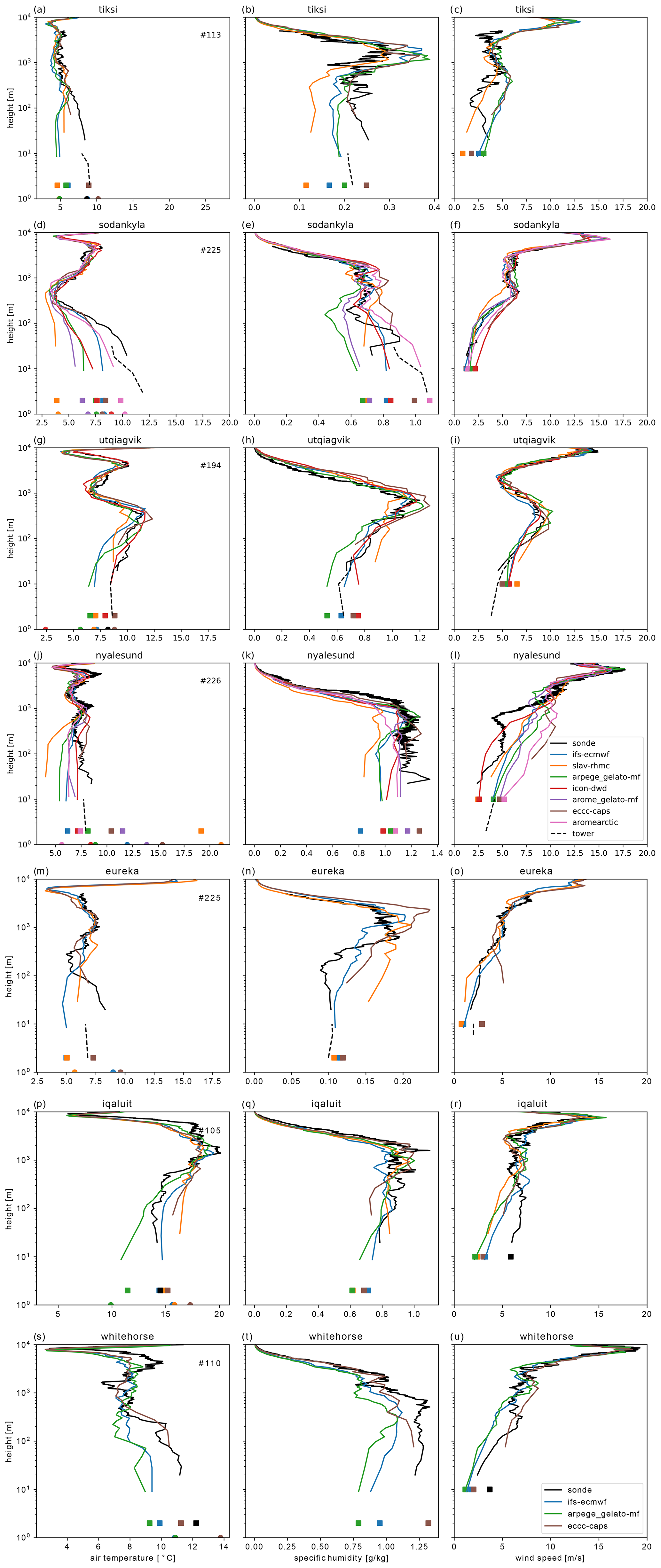
To gain further insights we investigate the vertical structure of the errors by comparing the model output to observations from radiosonde and tower. To do this the model and tower data were thinned to the same frequency as the radiosonde prior to calculating the median and inter-quartile range shown in Figs. 4 and 5. The median temperature and specific humidity within the boundary layer is overestimated at Tiksi, Eureka, Utqiaġvik and Iqaluit (see Fig. 4), and the models underestimate the strength of temperature and humidity inversions as a result. The picture is more mixed at Ny-Ålesund and Sodankylä where most models are too cold and humid, and two out of the three models are too dry at Whitehorse.
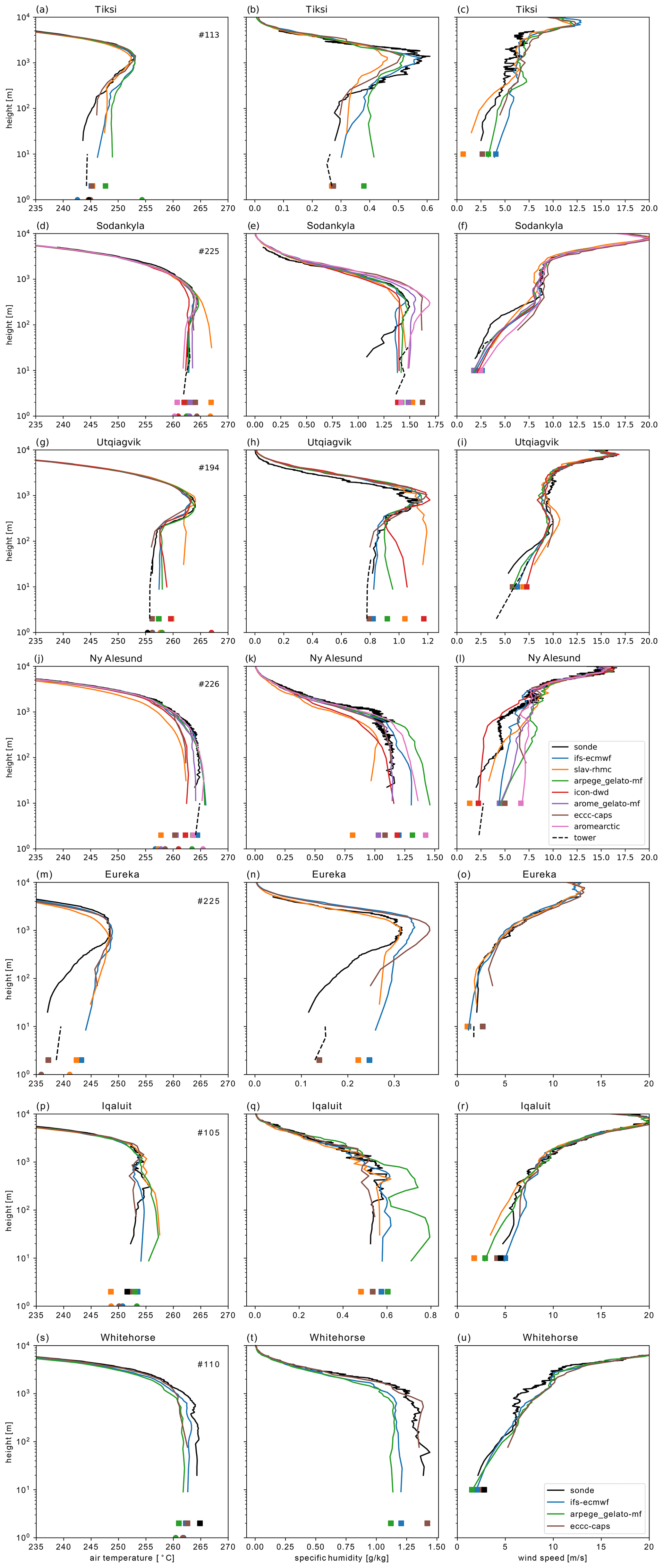
Figure 4Median temperature (left), specific humidity (middle) and wind speed (right) from the radiosonde (solid black line), the tower (dashed black line), and the numerical models (during the second day of the forecast: colour lines). The mean surface skin temperature is indicated by a dot and 2 m temperature (left), 2 m specific humidity (middle) and 10 m wind speed (right) are shown with a square. Note that wind speed and humidity profiles from the tower are not available in the Tiksi and Ny-Ålesund MODFs, respectively. The numbers in the left-hand panels correspond to the verification sample size, which was dictated by the availability of radiosonde profiles.
The biases in the upper-air temperatures, 2 m air temperature and the surface skin temperature tend to go hand in hand, i.e. the model with the warmest or coldest surface temperature tends to have the warmest or coldest 2 m and upper-air temperatures. As a result, the mean 2 m temperature errors seen in Fig. 2 give a sense of the sign of the error in the lowest 100 m or so of the atmosphere. This coupling between the lowest model level, the surface skin temperature and the 2 m temperature is to be expected since the 2 m temperature is a diagnostic calculated as a function of the lowest atmospheric model layer and the surface skin temperature.
Air temperature variability in the lower boundary layer is generally underestimated by the models, except at Iqaluit (Fig. 5). This generally translates to an underestimation of the 2 m temperature variability at these sites. Interestingly, at Ny-Ålesund some models severely overestimate the 2 m temperature variability despite underestimating the variability aloft, possibly due to the overestimation of the surface skin temperature variability. For specific humidity the observed inter-quartile range tends to sit within the range of the models; however, it is overestimated at Eureka and underestimated at Tiksi and Whitehorse in the lower boundary layer.
The median of the modelled wind speed is too high in the boundary layer at Sodankylä, Utqiaġvik and Tiksi but more mixed at other sites (Figs. 4 and 5). The variability in the wind speed is within the model range, with the exception of Iqaluit, where it is underestimated. The overestimation of the wind speed at these sites is likely a contributing factor in the underestimation of the temperature and humidity inversions, since a positive bias in the wind speed will drive excessive turbulent mixing of heat and moisture inhibiting the decoupling of near-surface and upper-air temperatures that occurs during periods of radiative surface cooling and low wind (Van de Wiel et al., 2017). Other factors which could play a role are the radiative forcing at the surface or the response of the surface to radiative forcing. Both aspects will be addressed in the following subsection.
3.3 Links between errors in boundary layer temperature variability and surface radiation
In this section we investigate the role of radiative forcing in the underestimation of near-surface and boundary-layer temperature variability at Sodankylä, Utqiaġvik and Tiksi where the models underestimate the temperature variability. At these sites all upwelling and downwelling radiation components are available in the NH-SOP1 MODFs allowing us to investigate whether the suppressed temperature variability is related to suppressed variability in the radiative forcing at the surface, a lack of sensitivity of the near-surface temperature to radiative forcing or something else.
The boxplots shown in Fig. 6a–c confirm the underestimate of near-surface temperature inter-quartile range (IQR) at Tiksi (except CAPS), Sodankylä, and Utqiaġvik, and further show that the cold tail of the distribution is generally shorter in the models meaning there is a warm bias during cold periods. The warm bias in cold conditions is well known at Sodankylä and is typical of NWP systems (see Atlaskin and Vihma, 2012, and Day et al., 2020), but this feature has not been shown before at the other two sites to our knowledge.
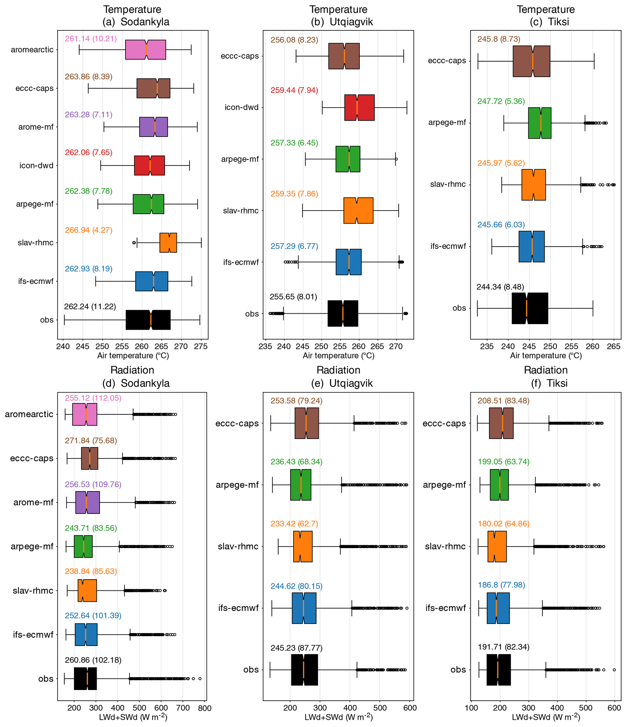
Figure 6Boxplots of T2m (a–c) and LW↓ + SW↓ (d–f) for Sodankylä, Utqiaġvik and Tiksi in observations and during the second day of the forecast. The text above the boxplots states the median (and inter-quartile range) of each distribution, which are also shown by the orange line and box edges, respectively. The 5 %–95 % range is plotted by the whiskers and points outside this are shown in dots.
The models typically also show differences in the distribution of the downwelling radiation at the surface, LW↓ + SW↓ compared to observations (Fig. 6d–f). The IQR is underestimated at Tiksi (except for CAPS) and Utqiaġvik. However, at Sodankylä all the models overestimate the IQR (except for CAPS) but also do not capture the highest values of incident radiation observed at the top of the distribution. Since errors in the incident radiation likely relate to interactions with clouds, which are not included in this iteration of the MODFs, we will not investigate the causes of these discrepancies between the observed and forecast radiation distributions further, leaving this for a more focussed future study, and we will instead move on to focus on the response of the near-surface air temperature and the surface energy budget.
As LW↓ + SWnet is the effective radiative forcing for the surface skin temperature (and indirectly for the 2 m temperature), errors in 2 m air temperature are either due to errors in this driving term itself, the relationship between LW↓ + SWnet and 2 m temperature, or more likely a combination of both (assuming that errors in advection are negligible). Because the model median surface albedo (except for SLAV at Tiksi) is close to the observed estimate (Fig. 7), we can focus on how 2 m temperature varies as a function of LW↓ + SWnet, to more deeply investigate the causes of error.
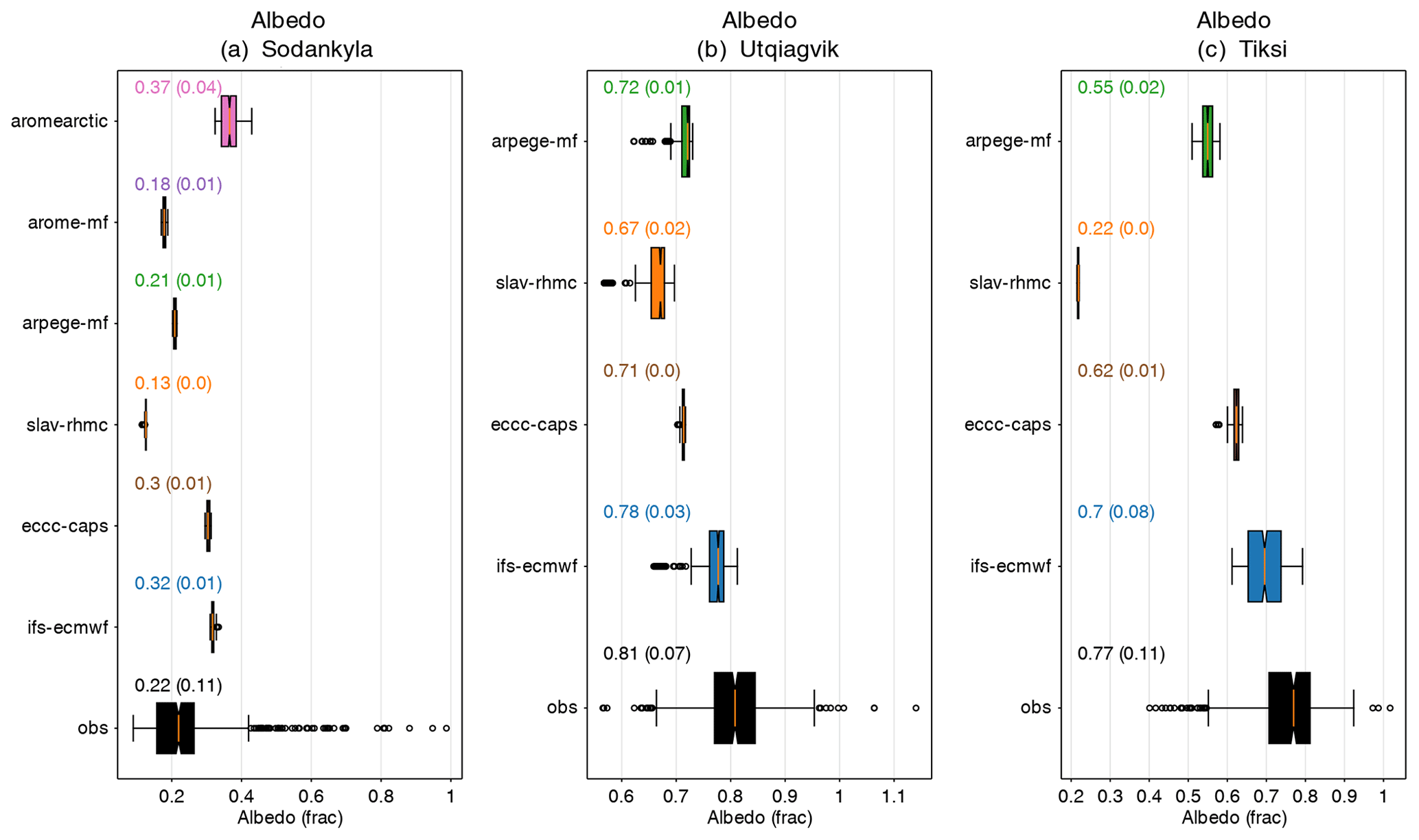
Figure 7Boxplots of surface albedo for Sodankylä, Utqiaġvik and Tiksi in observations and during the second day of the forecast. The text above the boxplots states the median (and inter-quartile range) of each distribution, which are also shown by the orange line and box edges, respectively. The 5 %–95 % range is plotted by the whiskers and points outside this are shown in dots.
At Sodankylä, Tiksi and Utqiaġvik all the models have a warm 2 m temperature bias at low levels of incoming radiation (LW↓ + SWnet) (see Fig. 8). At Tiksi, Utqiaġvik and Sodankylä the overall sensitivity of T2m to radiative forcing, as measured by the slope of the regression coefficient between 2 m temperature and LW↓ + SWnet is underestimated in all the models with one exception. The AROME-Arctic model seems to be too sensitive at Sodankylä according to this diagnostic, but it captures the observed temperature range at low levels of LW↓ + SWnet.
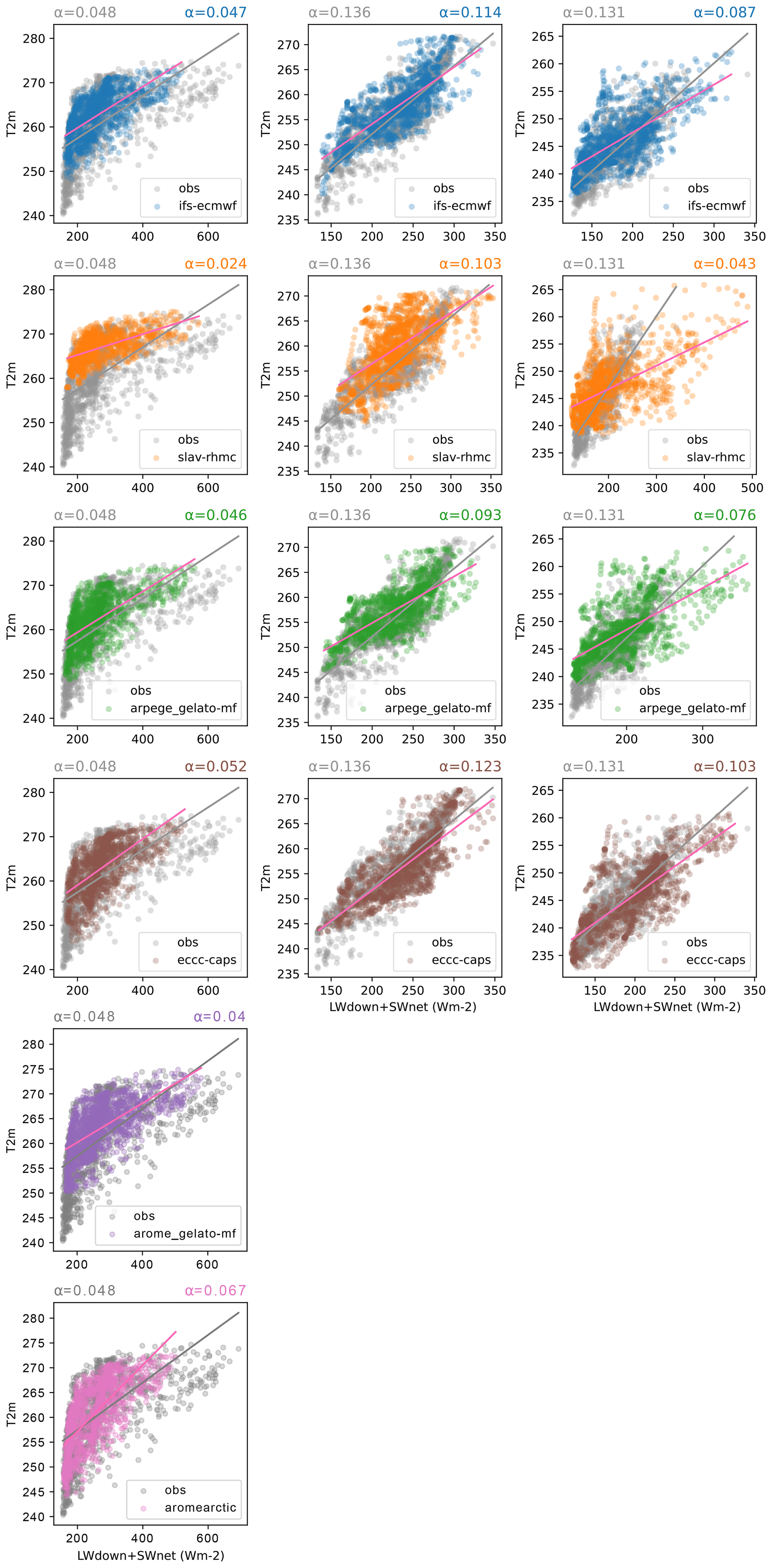
Figure 8Scatterplots of 2 m temperature as a function of LW↓ + SWnet for Sodankylä, Utqiaġvik and Tiksi (from left to right) for the second day of the forecast. The regression slope between the 2 m temperature and the LW↓ + SWnet is stated in the title for the observations (in grey) and each model (various colours).
Note that the LW components used for Sodankylä in this study are not those provided in the NH-SOP1 MODF, which are collected at the top of the 45 m tower, rather they are from a dedicated radiation tower located near the sounding station where the downwelling component is at a height of 16 m and the outgoing is at 2 m. These were swapped due to a concern over the accuracy of the LW radiation data collected at the met tower (Roberta Pirazzini, personal communication, 2023).
To investigate the role of surface–atmosphere decoupling in the 2 m temperature cold-tail warm bias and lack of 2 m temperature variability at low levels of incident radiation, we plot the thermal stratification as a function of near-surface wind speed at the three sites (Fig. 9) for situations where the model or observed LW↓ + SWnet is below the 20th percentile. In the observations one can see the typical pattern seen at other sites (e.g. Van de Wiel et al., 2017) that shows that inversions are weak for strong winds, whereas large inversions are found under weak wind conditions with a transition found between those regimes at some critical wind speed. The models generally capture this qualitative regime behaviour (Fig. 9), although the magnitude of the thermal stratification, the wind speed and the critical wind speed for the regime transition varies between the models.
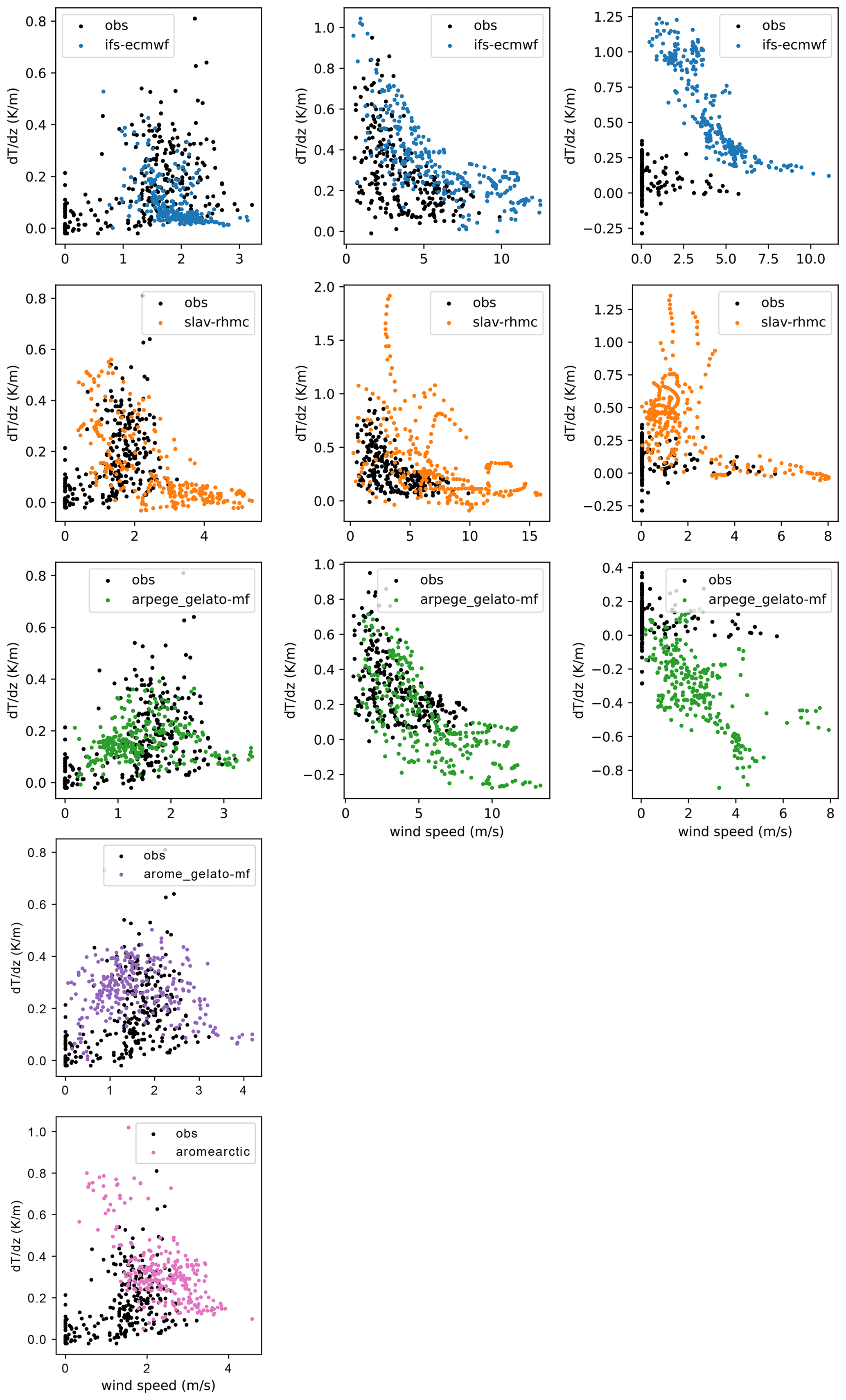
Figure 9Scatterplots of thermal stratification () as a function of wind speed on the lowest model at Sodankylä, Utqiaġvik and Tiksi (from left to right) for the observations (in black) and each model (various colours) during the second day of the forecast for situations where the model or observed LW↓ + SWnet is below the 20th percentile.
3.4 Surface energy budget sensitivity to radiative forcing
Further insight into the role of the land surface and surface exchange processes in the T2m errors outlined in the previous section, particularly the lack of T2m sensitivity to radiative forcing, can be gained by constructing surface energy budget sensitivity diagrams, following Miller et al. (2018) and Day et al. (2020). The idea here is that the surface energy budget can be separated into a “driving term” (LW↓ + SWnet) and “response terms” (sensible heat flux (SHF), latent heat flux (LHF), ground heat flux (GHF), and LW↑). The relationship between the driving term and each response term can be summarised with regression coefficients; e.g. for the SHF the following equation is used:
where each of the α values can be interpreted as a coupling strength parameter between the driving term and each response term. These α values provide direct information on the proportional response of each flux term, expressed as a fraction of the total change in radiative forcing. From this one can see that if, for example, the coupling to the ground heat flux and turbulent fluxes is too strong in the model (i.e. ), |αLW↑| will be too small, meaning that the surface temperature response will be too weak (and vice versa). Similarly, compensating errors in the strength of the coupling to the turbulent fluxes () and ground heat flux () could result in the right surface temperature sensitivity, αLW↑ but for the wrong reasons. As a result, by comparing the observed and modelled regression coefficients one can derive physical understanding of the causes of model error.
Note that in convective cases the main driver of turbulent heat fluxes is indeed the convective instability at the surface driven by radiative forcing. However, in stratified conditions the main driver of turbulence in the boundary layer (and of the sensible and latent heat fluxes) is the mechanical forcing, i.e. the large-scale wind speed (Van Hooijdonk et al., 2015; Van de Wiel et al., 2017; Vignon et al., 2017). As a result, one expects the turbulent fluxes to have little sensitivity to the radiative forcing in stable conditions, with the ground heat flux taking a larger role in balancing changes in radiative forcing and the converse in convective cases (see Day et al., 2020). As a result, at Utqiaġvik and Tiksi where stable conditions dominate, the ground heat flux varies with changes in radiative forcing more than the turbulent fluxes, as indicated by higher regression coefficients. At Sodankylä there is more of an even partitioning between the turbulent fluxes and the ground heat flux into the snow.
It is clear from Figs. 10–12 that all the models generally underestimate the surface temperature sensitivity to radiative forcing at Sodankylä, Utqiaġvik and Tiksi because the rate of change in LW↑ with changes in radiative forcing, LW↓ + SWnet, i.e. αLW↑, is typically too low (i.e. ). Since the 2 m temperature diagnostic in the models is calculated as a function of the surface skin temperature, the underestimation of the 2 m temperature and LW↑ sensitivity to radiative forcing and the positive bias in those variables in cold conditions are likely to be closely related (i.e. comparing Fig. 8 to Figs. 10–12). For example, at Sodankylä the CAPS model T2m and upwelling longwave (LW↑) sensitivities are very close to what is observed, AROME-Arctic slightly overestimates these sensitivities while SLAV underestimates them. A similar proportionality can be seen between these properties of the models at the other two sites. Note that because the LW↑ at Sodankylä was observed at 2 m and thus has a rather small footprint compared to the sensor on the 16 m mast, the sensitivity is more representative of the bare snow than the forest canopy. As a result, one might expect the area mean LW↑ sensitivity to be higher than the value presented here.
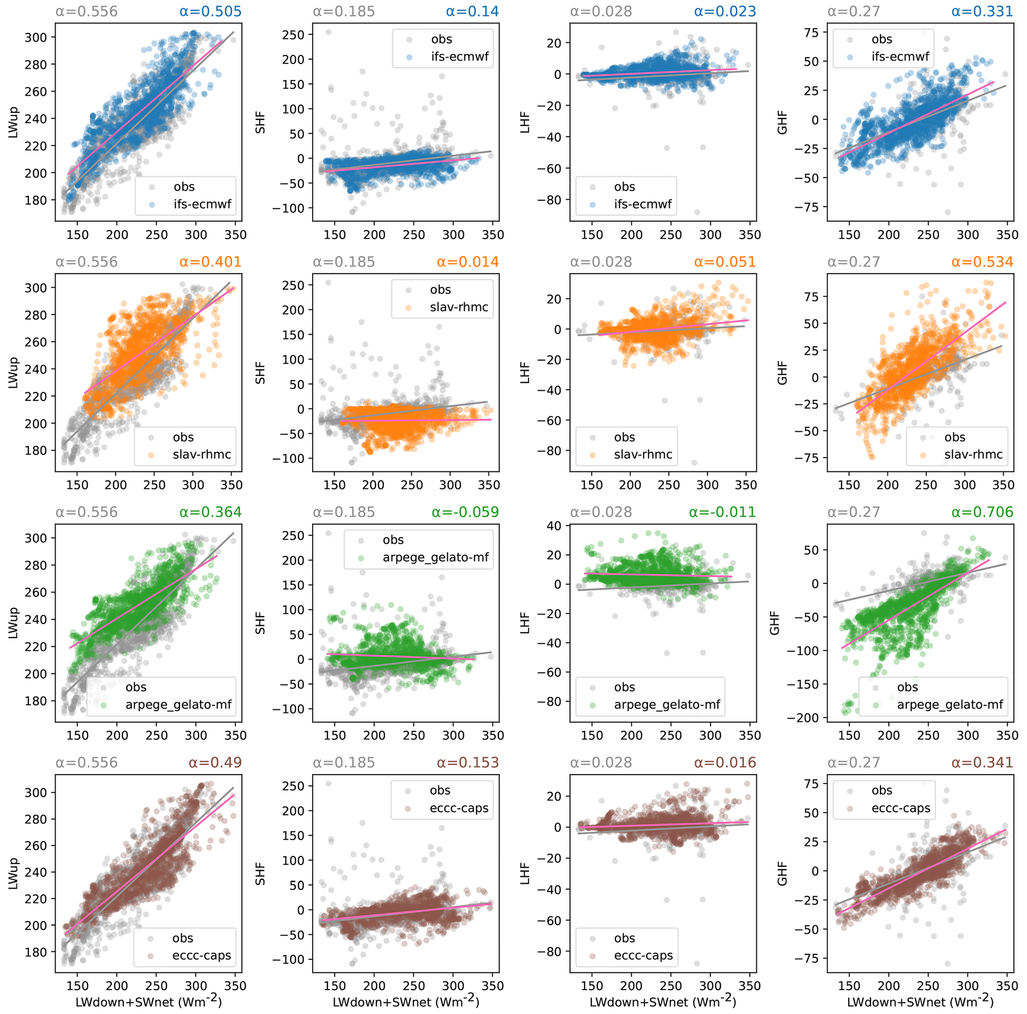
Figure 10Process relationship diagrams and sensitivity parameters for upwelling longwave radiation (LW↑; left), sensible heat flux (SHF; middle left), latent heat flux (LHF; middle right) and ground heat flux (GHF; right) at Utqiaġvik. Observed values are shown in grey, model values during the second day of the forecast are shown in colour. The line of best linear fit is shown for observations (grey line) and each model (pink line). The sensitivity parameters, α, describing the coupling strength between the driving (LW↓ + SWnet) and each response term are printed above each diagram, with the observational (modelled) relationship on the left (right).
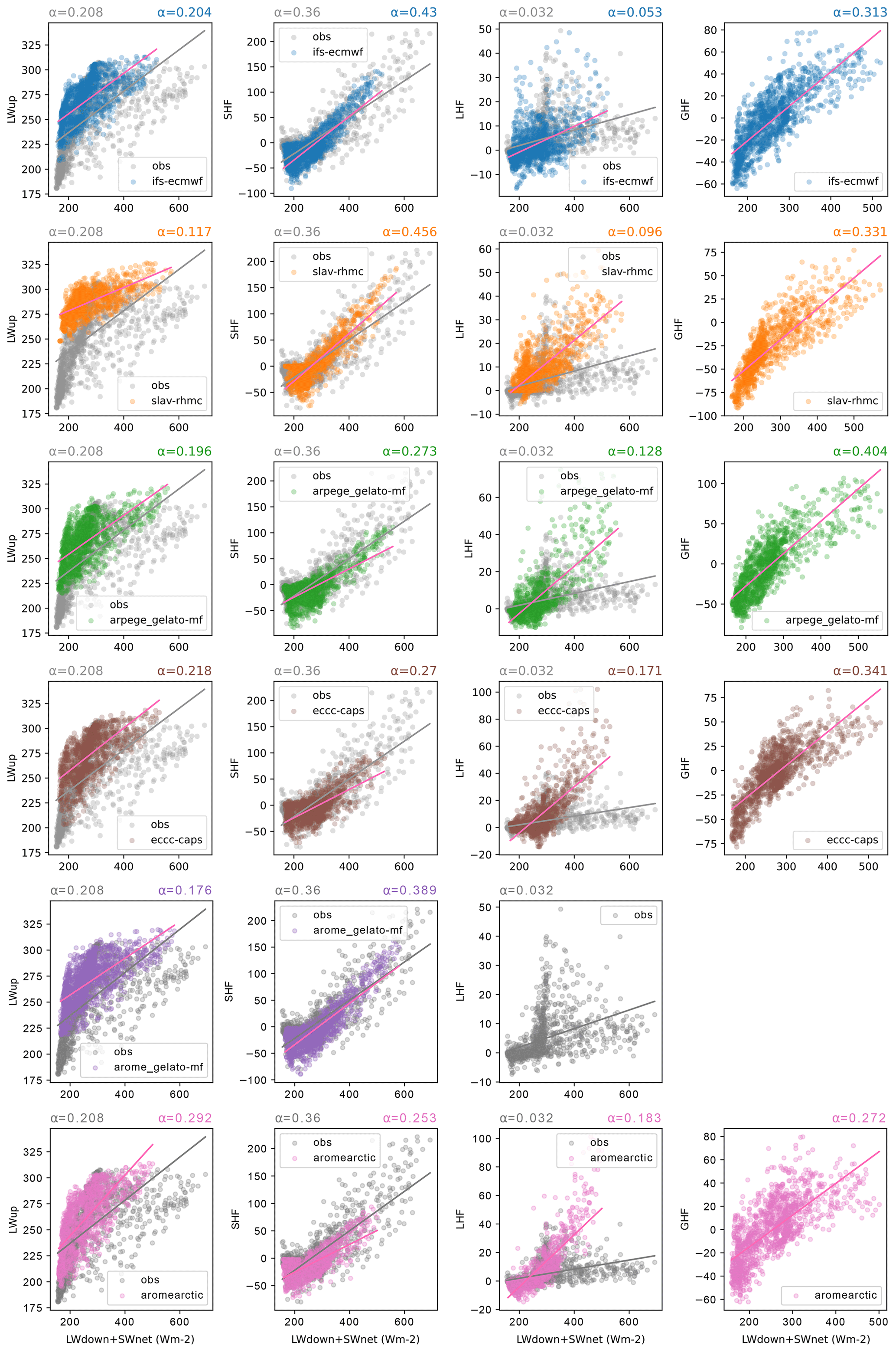
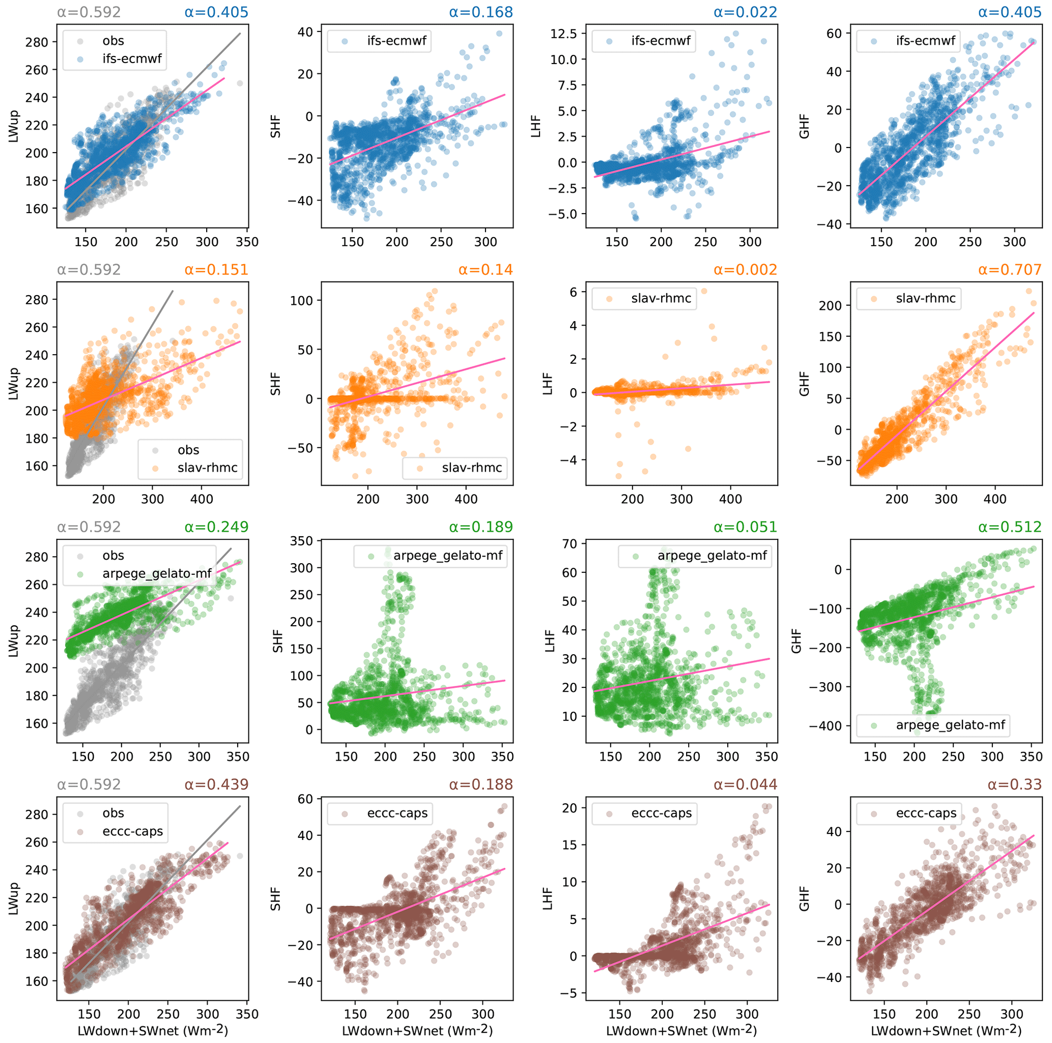
This mismatch in terms of LW↑ sensitivity goes hand in hand with differences in the other α coefficients, and by comparing the sensitivities of the other response terms in the surface energy budget we can develop some hypotheses about what is leading to this mismatch in surface temperature sensitivities. For example, at Utqiaġvik, all the models tend to overestimate the sensitivity of the GHF, αGHF, which was calculated as the residual of the observed radiative and turbulent fluxes. This can be an indication of non-sufficient thermal representation of the land surface, e.g. a lack of a multi-layer snow model (e.g. Day et al., 2020; Arduini et al., 2019). Unfortunately, we are not able to perform a similar calculation to that performed for Sodankylä to estimate the GHF, as the longwave observations thought to be most reliable are not co-located with the other flux observations, or at Tiksi, as we do not have the turbulent fluxes in the MODF. As a result, we cannot calculate the GHF as a residual of the other terms.
Where we have turbulent flux observations, we can also evaluate the αSHF and αLHF terms. At Utqiaġvik, an underestimation of the sensitivity of the turbulent fluxes, too low αSHF and αLHF in the ARPEGE and SLAV models goes hand in hand with an overestimation of αGHF mentioned above. The IFS and ECCC models are closer to observations, with smaller values of αGHF and larger values of αSHF and αLHF. At Sodankylä, the αSHF varies quite a bit from model to model, but all the models where the LHF was available overestimate the αLHF.
At all three sites the relative size of the coefficients varies, with αLW↑, αSHF and αGHF typically being an order of magnitude larger than αLHF. This is likely to be typical of cold and dry snow-covered environments where the magnitude of the latent heat flux is low. However, the difference in the relative size of the other three terms varies quite a bit between sites with, for example, the turbulent flux playing a larger role at Sodankylä than at Tiksi and Utqiaġvik at this time of year. This reflects the larger surface roughness at Sodankylä associated with the trees at this site.
Before moving on it is worth noting that as well as being used to develop hypotheses about the causes of errors related to the surface energy budget, these process diagrams and sensitivity metrics could also be applied to test new configurations of NWP systems with modifications to the land surface, boundary layer or related schemes and evaluate whether such modifications are improving the dynamic behaviour with respect to the surface energy budget in line with observed behaviour or not.
3.5 Evaluation of wind stress and sensible heat flux
The previous examples highlight discrepancies between forecast and observations and provide hints as to which processes are responsible for the documented errors. The observed conditions also provide multi-variate targets for updated forecasting systems. However, the observations can also help us evaluate a specific process and thereby target a specific parameter or parameterisation to change.
The Sodankylä and Utqiaġvik MODFs include turbulent fluxes and profiles of wind speed and temperature, allowing us to investigate the parameterisation of turbulent exchanges of heat and momentum at the surface. Turbulent surface fluxes in NWP models are often parameterised according to Monin–Obukhov (M-O) similarity theory where they are related to the gradient in the lowest atmosphere (e.g. Beljaars and Holtslag, 1991):
where τ is the wind stress; U is the wind speed; θ is potential temperature; ρ is the air density and the transfer coefficients; and CM and CH, used to in each computation, are a function of the roughness length of momentum and heat, zoM and zoH, and a stability parameter. In these equations, Uref and θref are the wind speed and potential temperature at a reference height, respectively, which in the case of the models is the lowest atmospheric model level, the height of which varies from around 10 to 30 m above the surface depending on the model (see Table 3).
Successfully parameterising τ and SHF relies on defining a reasonable function for CM and CH and selecting the appropriate parameters and a proper aggregation of the fluxes in the cases of a tiled surface. Because we have observed and forecasted values for both the fluxes and the bulk parameters in Eqs. (2) and (3), we can diagnose how appropriate the choices in each model are for the conditions at a particular site. This is done by examining the relationship between the bulk parameters, U and θ, and the fluxes τ and SHF (see Figs. 13–16), as done previously by Tjernström et al. (2005) and more recently by Day et al. (2020).
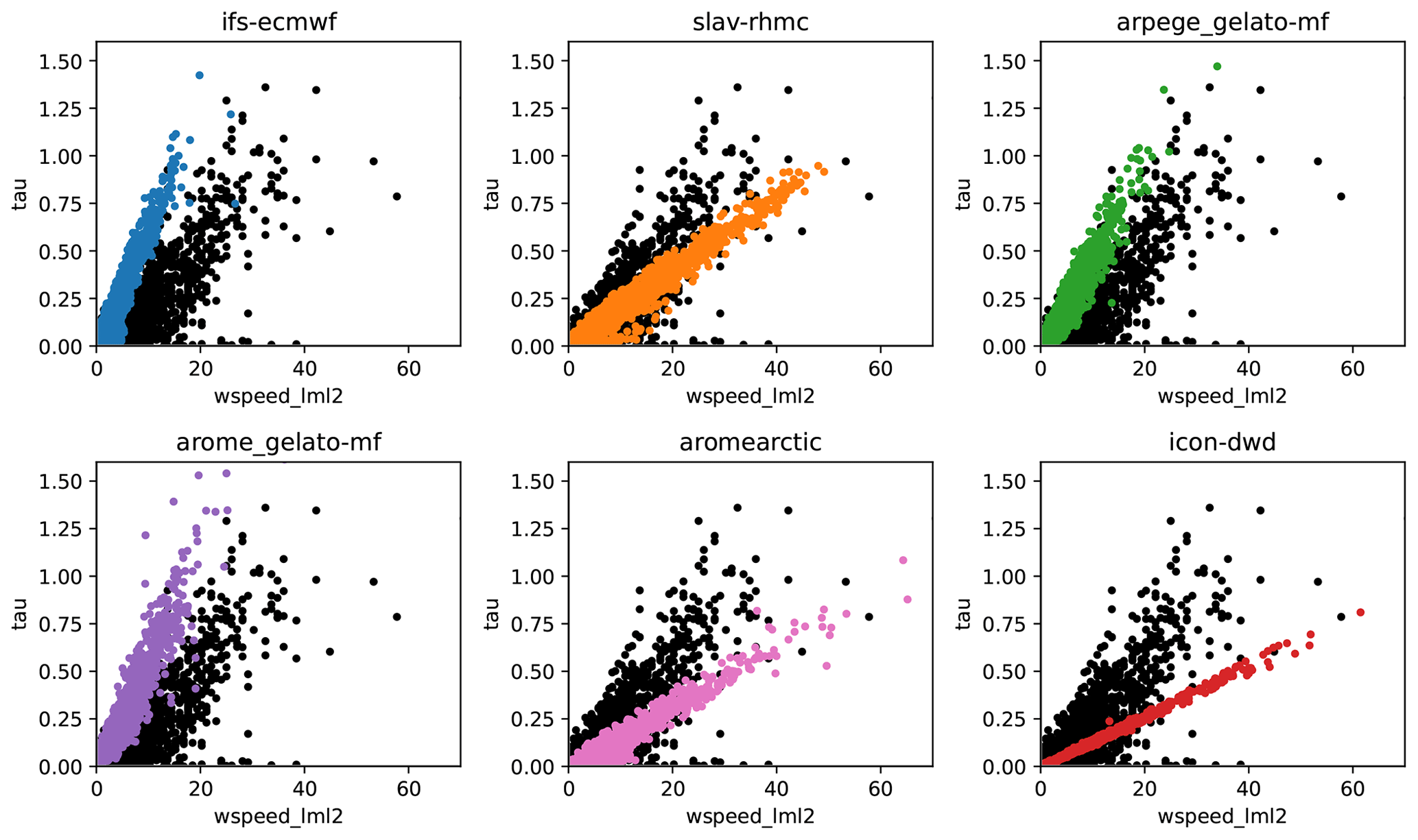
Figure 13Scatterplots of wind stress vs. the square of the near-surface (lowest model level) wind speed at Sodankylä. The observed points are shown in black, while hourly values during the second day of the forecast forecast are shown in colour.
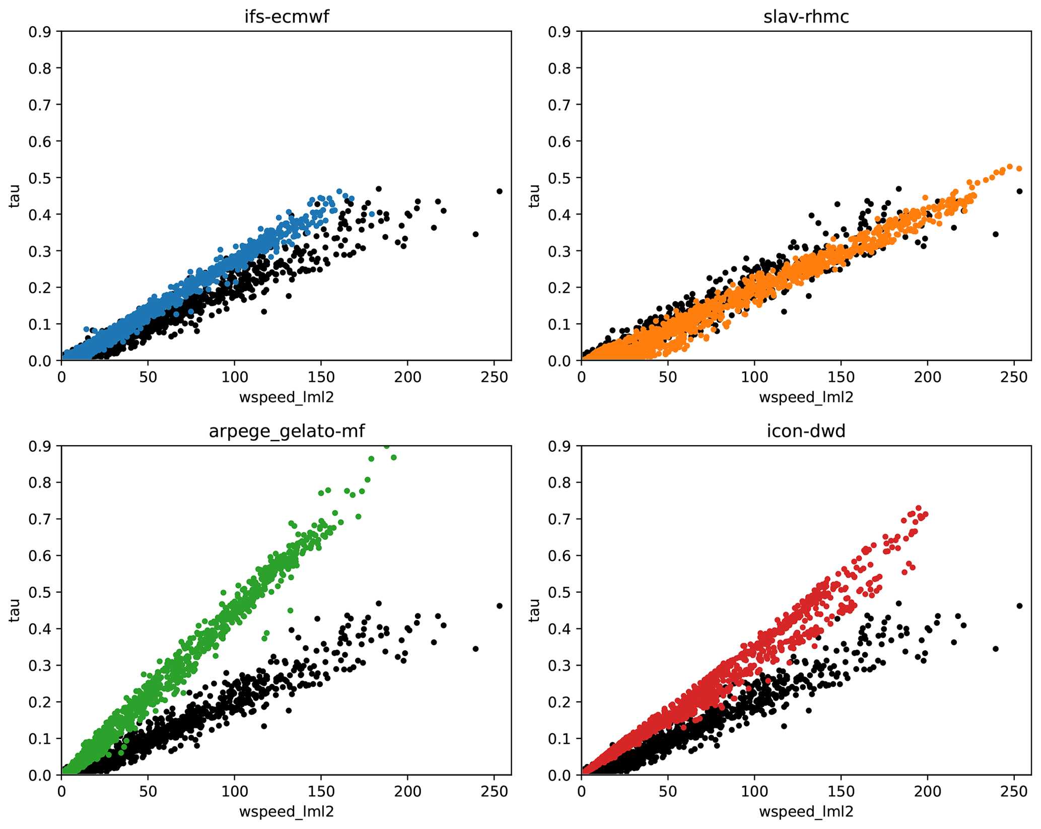
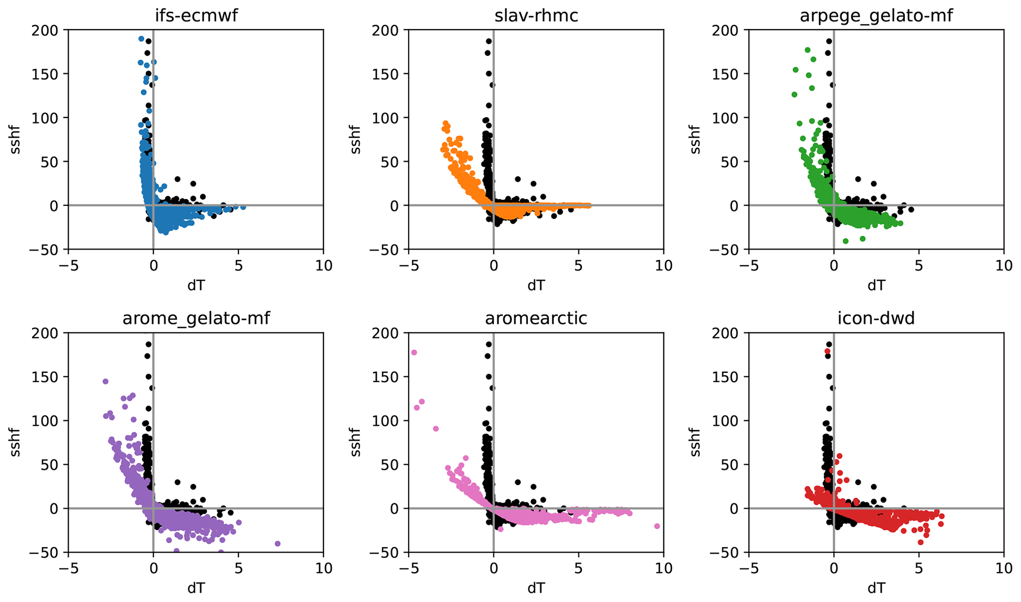
Figure 15Scatterplots of the scaled sensible heat flux () vs. thermal stratification, , at Sodankylä. The observed points are shown in black, while hourly values during the second day of the forecasts are shown in colour. Note that at Sodankylä the SHF is measured at 24.5 m, and for process consistency ΔT is calculated using the temperatures observed at 18 and 32 m, meaning that it is not directly comparable with the models that use the skin temperature, Tskin, and the lowest model level, Tlml.
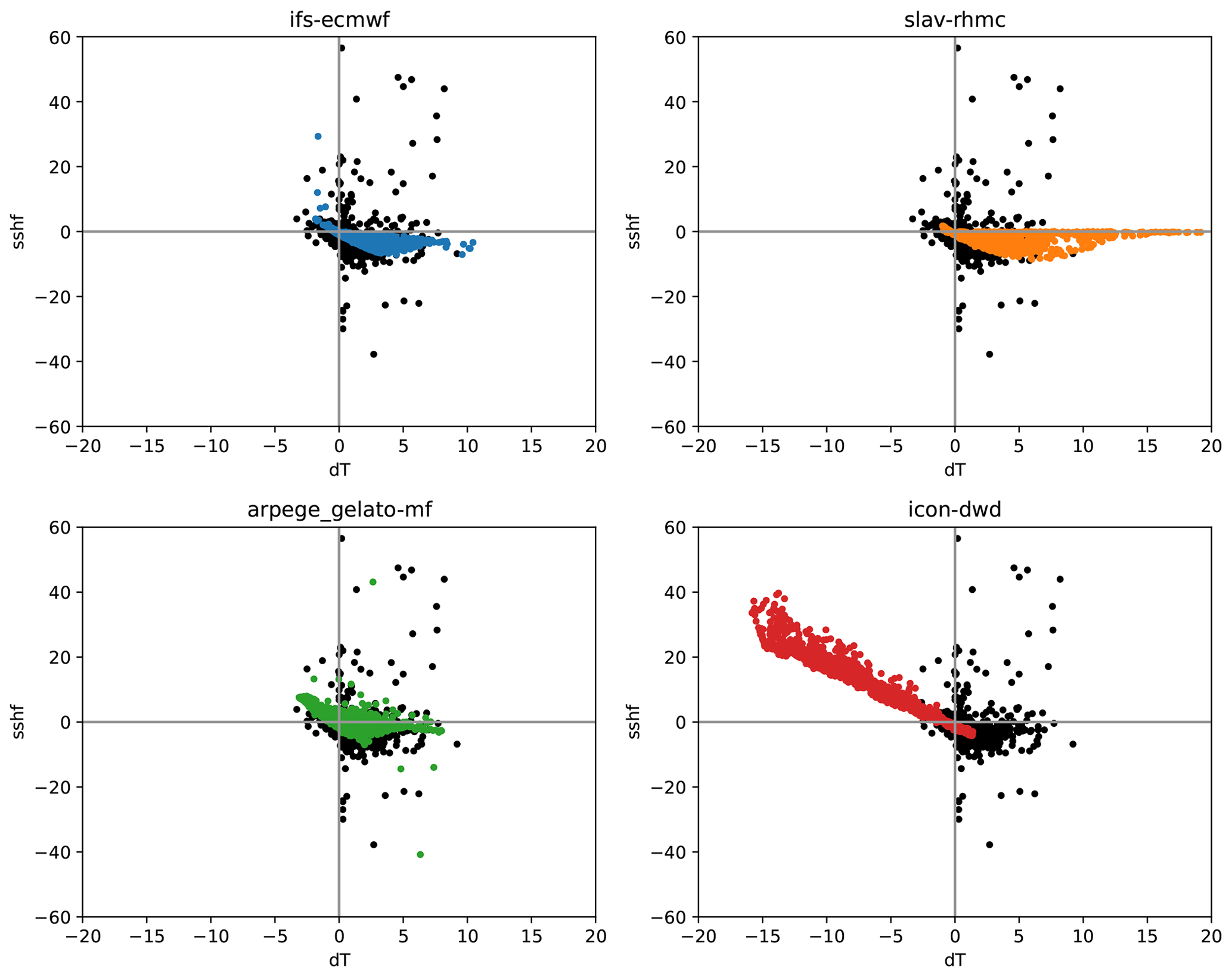
Figure 16The same as Fig. 15 but for Utqiaġvik. Note that for the observations ΔT is calculated using the 10 m air temperature and an estimate of the surface temperature from an infrared sensor.
In the case of wind stress, in neutral conditions, the points in Figs. 13 and 14 would sit on the straight line following
where zref is the height of the lowest model level, k is the von Kármán constant and z0m is the aerodynamic roughness length. The slope of this line is determined by z0m. However, this formula provides an overly simplified view as the atmospheric stability varies from neutral conditions, and as a result there is scatter in the values of τ for any given wind speed.
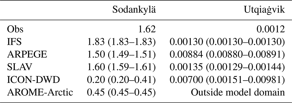
The relationship between τ and U for Sodankylä (Fig. 13) differs between the models and between the models and the observations. An estimate of the observed roughness length was calculated following the equation above after selecting for neutral conditions, and the value is presented in Table 4 along with the value used in each of the models. In the AROME-Arctic and ICON models, τ increases too slowly with increasing U. This is consistent with the fact that the roughness length for momentum is too low in these models, which have roughness lengths an order of magnitude lower than that derived from observations (see Table 4). Increasing z0m in the AROME-Arctic and ICON models would likely reduce the positive bias in the wind median wind speed profile seen in Fig. 4; however, the other models that have roughness lengths closer to what was observed also have a positive wind speed bias, suggesting another cause.
Table 4Roughness lengths for momentum (m) at Sodankylä and Utqiaġvik from observations and models. For the models the mean is stated, while the range of values is stated in parentheses.
Interestingly, all models fail to adequately capture the spread of τ for a given value of U, likely because the models underestimate the atmospheric stability as is suggested by the weaker than observed thermal stratification indicated by in Figs. 4d and 5d. A more detailed study including numerical experimentation would be needed to demonstrate this further.
At Utqiaġvik, the aerodynamic roughness length is 3 orders of magnitude lower than at Sodankylä, reflecting the difference in surface type: snow-covered tundra compared to the forested taiga of northern Finland (Table 4). Here the IFS and SLAV models have roughness lengths close to those derived from observations, whereas ARPEGE and ICON have values that are higher. As a result, for a given wind speed the surface stress is too high in these two models (Fig. 14).
The scatterplots for the sensible heat flux (Figs. 15 and 16) also provide some insights into the differences in the process representation between the models. All the models capture the link between the SHF and the temperature gradient, ΔT, dictated by M-O theory (see Eq. 3); however, the shape of the relationship varies between the models. For example, for the ARPEGE and AROME-MF models the sign of the sensible heat flux does not change in a binary way with ΔT, instead there is spread in the location along the x axis where this occurs. This could be due to differences in the numerical formulation of the models, i.e. the time step at which the flux and temperature terms are stored, or due to the fact that we are looking at the grid box mean values where the fluxes are aggregated from values computed on different surface tiles. At Sodankylä, the IFS, SLAV and AROME-ARCTIC model have a clear tapering in the scaled sensible heat flux towards zero for high values of ΔT. However, AROME-MF, ARPEGE and ICON do not have such a tapering, and the scaled heat flux continues to grow with larger ΔT, which is qualitatively inconsistent with the observations and will lead to higher fluxes in very stable conditions inhibiting cooling of the surface. There is also a clear difference in the range of ΔT between the different models; however, in the models this is an aggregate of different surface types representing forest canopy top, bare snow and frozen water, and because we do not have a trustable observation of the temperature of the top of the canopy frozen water during freezing conditions, it is not clear what the realistic range should be. Note also that the SHF at Sodankylä is measured at 24.5 m, and for process consistency ΔT is calculated using the air temperatures observed at 18 and 32 m, which is not directly comparable with the models.
Except for ICON, differences between the models at Utqiaġvik are less pronounced. IFS, SLAV and ARPEGE have quite a similar shape, and all underestimate the magnitude of the scaled heat flux for low values of ΔT, potentially due to the slow bias in wind speeds near the surface. Note that the large values of ΔT for the SLAV model are because the lowest model level is at ∼30 m compared to ∼10 m for the other models. Note that the ICON model has a large fraction of open ocean in the grid cell considered, and therefore the model tends to be biased towards convective conditions (i.e. most points are in the top-left quadrant of Fig. 16 where the sensible heat flux is heating the atmosphere), this is likely the main reason for the warm bias in surface skin temperature and 2 m air temperature. For the other models shown in Fig. 16, the grid point considered is 100 % land.
In this paper we have outlined the motivation for YOPPsiteMIP; documented the current status of the YOPPsiteMIP forecast MMDF data archived on the YOPP data portal (hosted by MET Norway); and presented some multi-model forecast evaluation examples to demonstrate the utility of the MMDFs and MODFs using data from the YOPP NH-SOP1, which occurred during February and March 2018. The main conclusions from this analysis are as follows.
-
Near-surface temperature and wind speed forecast errors vary considerably between the different sites, reflecting both a range of climate conditions and forecast performance across the selected sites.
-
A common feature of several sites, namely Sodankylä, Barrow, Tiksi and Eureka, is a warm bias during periods of extreme cold that goes hand in hand with a lack of temperature variability in the lowest ∼100 m of the atmosphere.
-
This lack of variability is investigated further at Utqiaġvik, Tiksi and Sodankylä where radiation components were observed and provided in the MODFs and MMDFs, which enabled us to investigate the sensitivity of T2m to radiative forcing.
-
At all three sites the models tend to underestimate the sensitivity of T2m and the surface skin temperature (or LW↑) to variations in radiative forcing and do not capture extreme minima in these variables, although the AROME-Arctic and CAPS models perform better in this regard.
-
-
At Utqiaġvik and Sodankylä, since turbulent fluxes were also provided, we were able to investigate the link between these fluxes and the bulk parameters. This highlighted the following points.
-
Differences were found in the parameterisation of turbulent fluxes, particularly the specification of the roughness length for momentum, which varies by a little less than an order of magnitude between different models.
-
The high importance of the atmosphere-to-snow heat flux was also noted, particularly at the Utqiaġvik and Tiksi sites, where stable conditions dominate. Note that despite this importance, this flux is not observed at these sites.
-
Process studies that compare point observations to gridded model output need to be carried out in awareness of sub-tile representativeness issues. For fine-resolution models it is always recommended to provide output from multiple grid points (as in this study) centred on the observatory to be able to pair land-based observations to a model tile with dominant land cover. For coarse-resolution models, we recommend providing variables for the different sub-tile components (bare soil, vegetation, water, ice, …). The more the site characteristics are matched to the correct model output, the more reliable diagnosis on the model capability to reproduce the observed physical process. In this study we found that the land–ocean contrast in the Arctic in winter does not significantly affect the surface energy budget sensitivity to radiative forcing in the CAPS model (in Sect. 3.4, the ocean-dominated Utqiaġvik grid points of CAPS do not stand out with respect to the other models) because the frozen ocean has similar characteristics to the snow-covered land surface. On the other hand, the ICON model, which has very low sea ice values (∼10 %), has much warmer temperatures than the other models at Utqiaġvik, and as a result the sensible heat flux behaves differently compared to the other models. Accounting for the land–ocean contrast will be crucial in the sea-ice-free summer NH-SOP2 period that will be evaluated in the future.
The development of the MODFs and MMDFs is ongoing and will be completed in phases. The initial phase was to collect basic meteorology data and the main components of the radiation budget. Work on this initial phase is completed, and the next phase will provide a wider range of parameters (e.g. turbulent fluxes and cloud parameters) included in the MODFs. This is a more complicated but very necessary step since the models differ significantly in terms of surface heat and momentum fluxes and cloud properties (not shown). There are also plans to extend the MODF and MMDF concept to Antarctica, focussing on the Southern Hemisphere SOPs. These future phases of the YOPPsiteMIP will allow more detailed studies of, for example, the following avenues:
-
cloud cover, microphysics, and radiative forcing;
-
assessment of forecast models in Antarctica;
-
testing of specific model developments;
-
observatory representativeness studies.
This will allow a more process-focussed understanding of the forecasts in the YOPPsiteMIP archive but also provide a test bed for model developers to use when testing new model formulations relevant for the Arctic. Further details on the MODF concept and the NH-SOP1 and NH-SOP2 MODFs can be found in Uttal et al. (2024) and Mariani et al. (2024), respectively. A Python-based toolkit for producing the MODFs is under development, and it is hoped will speed up and simplify the production of MODFs and facilitate timely evaluation of forecast models to inform the model development process.
| EDMF | Eddy diffusivity mass flux |
| FE | Finite element |
| FD | Finite difference |
| FV | Finite volume |
| H | Hydrostatic |
| HARATU | HARMONIE-AROME with RACMO Turbulence |
| HTESSEL | Hydrology-tiled ECMWF scheme for surface exchanges over land |
| ICE3 | Three-class ice parameterisation |
| IQR | Inter-quartile range |
| ISBA | Interactions between surface–biosphere–atmosphere |
| NH | Non-hydrostatic |
| SURFEX | Surface Externalisée |
| TERRA | Land Surface module of the ICON weather forecast model |
| TKE | Turbulent kinetic energy |
Apart from the ECMWF-IFS, for which an open-access version of the code is available here: https://confluence.ecmwf.int/display/OIFS (last access: 16 July 2024), the model codes are not open access.
All MMDF and MODFs are available on the YOPP Data Portal (https://yopp.met.no (last access: 16 July 2024), hosted by the Norwegian Meteorological Institute, for perpetuity (i.e. longer than 10 years). The YOPP Data Portal is relying on the Arctic Data Centre (https://adc.met.no, last access: 16 July 2024) for data stewarding and the YOPPSiteMIP data can be programmatically accessed using the machine interface for the Arctic Data Centre or can be accessed directly from https://thredds.met.no/thredds/catalog/alertness/YOPP_supersite/obs/catalog.html (last access: 16 July 2024) for the MODFs and https://thredds.met.no/thredds/catalog/YOPPSiteMIP-models/catalog.html (last access: 16 July 2024), for the MMDFs.
The NH-SOP1 and NH-SOP2 MODFs for each station shown in white in Fig. 1 has been assigned a separate DOI, as described in Mariani et al. (2024). In the case of the MMDFs a DOI is assigned to the data for each forecast model:
-
ECMWF-IFS: https://doi.org/10.21343/A6KA-7142 (Day, 2023);
-
ARPEGE-MF: https://doi.org/10.21343/T31Z-J391 (Bazile and Azouz, 2023a);
-
SLAV-RHMC: https://doi.org/10.21343/J4SJ-4N61 (Tolstykh, 2023);
-
DWD-ICON: https://doi.org/10.21343/09KM-BJ07 (Frank, 2023);
-
ECCC-CAPS: https://doi.org/10.21343/2BX6-6027 (Casati, 2023);
-
AROME-MF: https://doi.org/10.21343/JZH3-2470 (Bazile and Azouz, 2023b);
-
AROME-Arctic: https://doi.org/10.21343/47AX-MY36 (Remes, 2023).
The initial YOPPsiteMIP, MODF and MMDF concepts were developed by GS, JJD, BC, TU, SJK, LMH, AS and EB. JJD, BC, EB, NA, HF, TR, RF and MT produced or ran simulations to make MMDFs. TU, EA, MG, LXH, JH, ZM, SM, EO'C, IS, MG, JT and RP produced or were involved in the production of MODFs. LF, MDS and ØG were responsible for the YOPPsiteMIP archive hosted at MET Norway. JJD produced the figures and wrote the manuscript with comments and input from all co-authors.
The contact author has declared that none of the authors has any competing interests.
Publisher's note: Copernicus Publications remains neutral with regard to jurisdictional claims made in the text, published maps, institutional affiliations, or any other geographical representation in this paper. While Copernicus Publications makes every effort to include appropriate place names, the final responsibility lies with the authors.
This is a contribution to the Year of Polar Prediction (YOPP), a flagship activity of the Polar Prediction Project (PPP), initiated by the World Weather Research Programme (WWRP) of the World Meteorological Organisation (WMO). We acknowledge the WMO WWRP for its role in coordinating this international research activity. We would specifically like to thank Thomas Jung, Jeff Wilson and the wider PPP steering group for their tireless support of YOPPsiteMIP.
Jonathan J. Day was supported by European Union's Horizon 2020 Research and Innovation programme through grant agreement no. 871120 (INTERACTIII).
Mikhail Tolstykh was partially supported with Russian Science Foundation (grant no. 21-17-00254). Publisher's note: the article processing charges for this publication were not paid by a Russian or Belarusian institution.
Roberta Pirazzini was supported by European Union's Horizon 2020 Research and Innovation program through grant agreement no. 101003590 (PolarRES).
Teresa Remes was supported by the Norwegian Research Council project no. 280573 “Advanced models and weather prediction in the Arctic: enhanced capacity from observations and polar process representations (ALERTNESS)”.
This paper was edited by Steven Phipps and reviewed by two anonymous referees.
Akish, E. and Morris, S.: MODF for Eureka, Canada, during YOPP SOP1 and SOP2, Norwegian Meteorological Institute, https://doi.org/10.21343/R85J-TC61, 2023a.
Akish, E. and Morris, S.: MODF for Tiksi, Russia, during YOPP SOP1 and SOP2, Norwegian Meteorological Institute, https://doi.org/10.21343/5BWN-W881, 2023b.
Akish, E. and Morris, S.: MODF for Utqiagvik, Alaska, during YOPP SOP1 and SOP2, Norwegian Meteorological Institute, https://doi.org/10.21343/A2DX-NQ55, 2023c.
Arduini, G., Balsamo, G., Dutra, E., Day, J. J., Sandu, I., Boussetta, S., and Haiden, T.: Impact of a multi-layer snow scheme on near-surface weather forecasts, J. Adv. Model. Earth Sy., 11, 4687–4710, https://doi.org/10.1029/2019MS001725, 2019.
Atlaskin, E. and Vihma, T.: Evaluation of NWP results for wintertime nocturnal boundary-layer temperatures over Europe and Finland, Q. J. Roy. Meteor. Soc., 138, 1440–1451, https://doi.org/10.1002/qj.1885, 2012.
Baldauf, M., Seifert, A., Förstner, J., Majewski, D., Raschendorfer, M., and Reinhardt, T.: Operational convective-scale numerical weather prediction with the COSMO model: description and sensitivities, Mon. Weather Rev., 139, 3887–3905, 2011.
Balsamo, G., Beljaars, A., Scipal, K., Viterbo, P., van den Hurk, B., Hirschi, M., and Betts, A. K.: A revised hydrology for the ECMWF model: verification from field site to terrestrial water storage and impact in the integrated forecast system, J. Hydrometeorol., 10, 623–643, https://doi.org/10.1175/2008JHM1068.1, 2009.
Batrak, Y. and Müller, M.: On the warm bias in atmospheric reanalyses induced by the missing snow over Arctic sea-ice, Nat. Commun., 10, 4170, https://doi.org/10.1038/s41467-019-11975-3, 2019.
Bauer, P., Magnusson, L., Thépaut, J.-N., and Hamill, T. M.: Aspects of ECMWF model performance in polar areas, Q. J. Roy. Meteor. Soc., 142, 583–596, https://doi.org/10.1002/qj.2449, 2016.
Bazile, E. and Azouz, N.: Merged model data files (MMDFs) for the Météo-France ARPEGE global forecast model for various polar sites, Norwegian Meteorological Institute [data set], https://doi.org/10.21343/T31Z-J391, 2023a.
Bazile, E. and Azouz, N.: MMDFs for the Météo-France AROME regional forecast model for various Arctic sites, Norwegian Meteorological Institute [data set], https://doi.org/10.21343/JZH3-2470, 2023b.
Bazile, E., Marquet, P., Bouteloup, Y., and Bouyssel, F.: The Turbulent Kinetic Energy (TKE) scheme in the NWP models at Météo-France, ECMWF GABLS Workshop on Diurnal Cycles and the Stable Boundary Layer, Reading, 7–10 November, 127–136, 2011.
Bazile, E., Azouz, N., Napoly, A., and Loo, C.: Impact of the 1D sea-ice model GELATO in the global model ARPEGE, France, 6–03, http://bluebook.meteoinfo.ru/index.php?year=2020&ch_=2 (last access: 11 July 2024), 2020.
Bechtold, P., Bazile, E., Guichard, F., Mascart, P., and Richard, E.: A mass flux convection scheme for regional and global models, Q. J. Roy. Meteor. Soc., 127, 869–886, 2001.
Bechtold, P., Köhler, M., Jung, T., Doblas-Reyes, F., Leutbecher, M., Rodwell, M. J., Vitart, F., and Balsamo, G.: Advances in simulating atmospheric variability with the ECMWF model: from synoptic to decadal time-scales, Q. J. Roy. Meteor. Soc., 134, 1337–1351, https://doi.org/10.1002/qj.289, 2008.
Bélair, S., Brown, R., Mailhot, J., Bilodeau, B., and Crevier, L.: Operational implementation of the ISBA land surface scheme in the Canadian regional weather forecast model. Part II: Cold season results, J. Hydrometeorol., 4, 371–386, 2003.
Bélair, S., Mailhot, J., Girard, C., and Vaillancourt, P.: Boundary layer and shallow cumulus clouds in a medium-range forecast of a large-scale weather system, Mon. Weather Rev., 133, 1938–1960, https://doi.org/10.1175/MWR2958.1, 2005.
Beljaars, A. C. M. and Holtslag, A. A. M.: Flux parameterization over land surfaces for atmospheric models, J. Appl. Meteorol., 30, 327–341, https://doi.org/10.1175/1520-0450(1991)030<0327:FPOLSF>2.0.CO;2, 1991.
Bengtsson, L., Andrae, U., Aspelien, T., Batrak, Y., Calvo, J., de Rooy, W., Gleeson, E., Hansen-Sass, B., Homleid, M., Hortal, M., Ivarsson, K.-I., Lenderink, G., Niemelä, S., Nielsen, K. P., Onvlee, J., Rontu, L., Samuelsson, P., Muñoz, D. S., Subias, A., Tijm, S., Toll, V., Yang, X., and Køltzow, M. Ø.: The HARMONIE–AROME model configuration in the ALADIN–HIRLAM NWP system, Mon. Weather Rev., 145, 1919–1935, https://doi.org/10.1175/MWR-D-16-0417.1, 2017.
Bougeault, P.: Cloud ensemble relations for use in higher order models of the planetary boundary layer, J. Atmos. Sci., 39, 2691–2700, 1982.
Bougeault, P.: A simple parameterisation of the large scale effects of cumulus convection, Mon. Weather Rev., 113, 2108–2121, https://doi.org/10.1175/1520-0493(1985)113<2108:ASPOTL>2.0.CO;2, 1985.
Bromwich, D. H., Werner, K., Casati, B., Powers, J. G., Gorodetskaya, I. V., Massonnet, F., Vitale, V., Heinrich, V. J., Liggett, D., Arndt, S., Barja, B., Bazile, E., Carpentier, S., Carrasco, J. F., Choi, T., Choi, Y., Colwell, S. R., Cordero, R. R., Gervasi, M., Haiden, T., Hirasawa, N., Inoue, J., Jung, T., Kalesse, H., Kim, S.-J., Lazzara, M. A., Manning, K. W., Norris, K., Park, S.-J., Reid, P., Rigor, I., Rowe, P. M., Schmithüsen, H., Seifert, P., Sun, Q., Uttal, T., Zannoni, M., and Zou, X.: The Year of Polar Prediction in the Southern Hemisphere (YOPP-SH), B. Am. Meteorol. Soc., 101, E1653–E1676, https://doi.org/10.1175/BAMS-D-19-0255.1, 2020.
Buizza, R., Bidlot, J.-R., Janousek, M., Keeley, S., Mogensen, K., and Richardson, D.: New IFS cycle brings sea-ice coupling and higher ocean resolution, ECMWF Newsl., 150, 14–17, https://doi.org/10.21957/xbov3ybily, 2017.
Casati, B.: MMDFs for the Environment and Climate Change Canada-CAPS regional forecast model for various Arctic sites, Norwegian Meteorological Institute [data set], https://doi.org/10.21343/2BX6-6027, 2023.
Casati, B., Robinson, T., Lemay, F., Køltzow, M., Haiden, T., Mekis, E., Lespinas, F., Fortin, V., Gascon, G., Milbrandt, J., and Smith, G.: Performance of the Canadian Arctic Prediction System during the YOPP Special Observing Periods, Atmosphere-Ocean, 61, 246–272, https://doi.org/10.1080/07055900.2023.2191831, 2023.
Catry, B., Geleyn, J. F., Bouyssel, F., Cedilnik, J., Brožková, R., and Derková, M.: A new sub-grid scale lift formulation in a mountain drag parameterisation scheme, Meteorol. Z., 17, 193–208, https://doi.org/10.1127/0941-2948/2008/0272, 2008.
Cheng, Y., Canuto, V. M., and Howard, A. M.: An Improved Model for the Turbulent PBL, J. Atmos. Sci., 59, 1550–1565, https://doi.org/10.1175/1520-0469(2002)059<1550:AIMFTT>2.0.CO;2, 2002.
Coté, J., Gravel, S., Méthot, A., Patoine, A., Roch, M., and Staniforth, A.: The operational CMC–MRD Global Environmental Multiscale (GEM) model. Part I: Design considerations and formulation, Mon. Weather Rev., 126, 1373–1395, https://doi.org/10.1175/1520-0493(1998)126<1373:TOCMGE>2.0.CO;2, 1998.
Cuxart, J., Bougeault, P., and Redelsperger, J.-L.: A turbulence scheme allowing for mesoscale and large-eddy simulations, Q. J. Roy. Meteor. Soc., 126, 1–30, https://doi.org/10.1002/qj.49712656202, 2000.
Cuxart, J., Holtslag, A. A. M., Beare, R. J., Bazile, E., Beljaars, A., Cheng, A., Conangla, L., Ek, M., Freedman, F., Hamdi, R., Kerstein, A., Kitagawa, H., Lenderink, G., Lewellen, D., Mailhot, J., Mauritsen, T., Perov, V., Schayes, G., Steeneveld, G.-J., Svensson, G., Taylor, P., Weng, W., Wunsch, S., and Xu, K.-M.: Single-Column Model Intercomparison for a Stably Stratified Atmospheric Boundary Layer, Bound.-Lay. Meteorol., 118, 273–303, https://doi.org/10.1007/s10546-005-3780-1, 2006.
Day, J.: MMDFs for the ECMWF-IFS global forecast model for various Polar sites, Norwegian Meteorological Institute [data set], https://doi.org/10.21343/A6KA-7142, 2023.
Day, J. J., Arduini, G., Sandu, I., Magnusson, L., Beljaars, A., Balsamo, G., Rodwell, M., and Richardson, D.: Measuring the Impact of a New Snow Model Using Surface Energy Budget Process Relationships, J. Adv. Model. Earth Sy., 12, e2020MS002144, https://doi.org/10.1029/2020MS002144, 2020.
Day, J. J., Keeley, S., Arduini, G., Magnusson, L., Mogensen, K., Rodwell, M., Sandu, I., and Tietsche, S.: Benefits and challenges of dynamic sea ice for weather forecasts, Weather Clim. Dynam., 3, 713–731, https://doi.org/10.5194/wcd-3-713-2022, 2022.
Delage, Y.: Parametrizing sub-grid scale vertical transport in atmospheric models under statically stable conditions, Bound.-Lay. Meteorol., 82, 23–48, https://doi.org/10.1023/A:1000132524077, 1997.
Delage, Y. and Girard, C.: Stability functions correct at the free convection limit and consistent for both the surface and Ekman layers, Bound.-Lay. Meteorol., 58, 19–31, https://doi.org/10.1007/BF00120749, 1992.
Donlon, C. J., Martin, M., Stark, J., Roberts-Jones, J., Fiedler, E., and Wimmer, W.: The Operational Sea Surface Temperature and Sea Ice Analysis (OSTIA) system, Remote Sens. Environ., 116, 140–158, https://doi.org/10.1016/j.rse.2010.10.017, 2012.
Ďurán, I. B., Geleyn, J., and Váňa, F.: A compact model for the stability dependency of TKE production–destruction–conversion terms valid for the whole range of Richardson numbers, J. Atmos. Sci., 71, 3004–3026, 2014.
Dyer, A. J. and Hicks, B. B.: Flux-Gradient Relationships in the Constant Flux Layer, Q. J. Roy. Meteor. Soc. 96, 715–721, 1970.
Emmerson, C. and Lahn, G.: Arctic opening: Opportunity and risk in the high north, Lloyds Rep., 59 pp., https://www.lloyds.com/news-and-insights/risk-reports/library/arctic-opening-opportunity-and-risk-in-the-high-north (last access: 11 July 2024), 2012.
Forbes, R. M. and Ahlgrimm, M.: On the Representation of High-Latitude Boundary Layer Mixed-Phase Cloud in the ECMWF Global Model, Mon. Weather Rev., 142, 3425–3445, https://doi.org/10.1175/MWR-D-13-00325.1, 2014.
Frank, H.: MMDFs for the DWD-ICON global forecast model for various Arctic sites, Norwegian Meteorological Institute [data set], https://doi.org/10.21343/09KM-BJ07, 2023.
Gerard, L. and Geleyn, J.-F.: Evolution of a subgrid deep convection parametrization in a limited-area model with increasing resolution, Q. J. Roy. Meteor. Soc., 131, 2293–2312, https://doi.org/10.1256/qj.04.72, 2005.
Gerard, L., Piriou, J., Brožková, R., Geleyn, J., and Banciu, D.: Cloud and Precipitation Parameterization in a Meso-Gamma-Scale Operational Weather Prediction Model, Mon. Weather Rev., 137, 3960–3977, https://doi.org/10.1175/2009MWR2750.1, 2009.
Girard, C., Plante, A., Desgagné, M., McTaggart-Cowan, R., Côté, J., Charron, M., Gravel, S., Lee, V., Patoine, A., Qaddouri, A., Roch, M., Spacek, L., Tanguay, M., Vaillancourt, P. A., and Zadra, A.: Staggered vertical discretization of the Canadian Environmental Multiscale (GEM) model using a coordinate of the log-hydrostatic-pressure type, Mon. Weather Rev., 142, 1183–1196, https://doi.org/10.1175/MWR-D-13-00255.1, 2014.
Goessling, H. F., Jung, T., Klebe, S., Baeseman, J., Bauer, P., Chen, P., Chevallier, M., Dole, R., Gordon, N., Ruti, P., Bradley, A., Bromwich, D. H., Casati, B., Chechin, D., Day, J. J., Massonnet, F., Mills, B., Renfrew, I., Smith, G., and Tatusko, R.: Paving the way for the Year of Polar Prediction, B. Am. Meteorol. Soc., 97, ES85–ES88, https://doi.org/10.1175/BAMS-D-15-00270.1, 2016.
Haiden, T., Sandu, I., Balsamo, G., Arduini, G., and Beljaars, A.: Addressing biases in near-surface forecasts, ECMWF Newsletter, 157, 20–25, https://doi.org/10.21957/eng71d53th, 2018.
Hartten, L. M. and Khalsa, S. J. S.: The H-K Variable SchemaTable developed for the YOPPsiteMIP, https://doi.org/10.5281/zenodo.6463464, 2022.
Heise, E., Ritter, B., and Schrodin, R.: Operational implementation of the multilayer soil model, COSMO Technical Reports no. 9, Consortium for Small-Scale Modelling, Offenbach am Main, Germany, https://doi.org/10.5676/DWD_pub/nwv/cosmo-tr_9, 2006.
Hogan, R. J. and Bozzo, A.: A Flexible and Efficient Radiation Scheme for the ECMWF Model, J. Adv. Model. Earth Sy., 10, 1990–2008, https://doi.org/10.1029/2018MS001364, 2018.
Holt, J.: Merged Observatory Data File (MODF) for Ny Alesund, Norwegian Meteorological Institute, https://doi.org/10.21343/Y89M-6393, 2023.
Holtslag, A. A. M. and De Bruin, H. A. R.: Applied Modeling of the Nighttime Surface Energy Balance over Land, J. Appl. Meteorol. Clim., 27, 689–704, 1988.
Holtslag, A. A. M., Svensson, G., Baas, P., Basu, S., Beare, B., Beljaars, A. C. M., Bosveld, F. C., Cuxart, J., Lindvall, J., Steeneveld, G. J., Tjernström, M., and Van De Wiel, B. J. H.: Stable Atmospheric Boundary Layers and Diurnal Cycles: Challenges for Weather and Climate Models, B. Am. Meteorol. Soc., 94, 1691–1706, 2013.
Huang, L., Mariani, Z., and Crawford, R.: MODF for Erik Nielsen Airport, Whitehorse, Canada during YOPP SOP1 and SOP2, Norwegian Meteorological Institute, https://doi.org/10.21343/A33E-J150, 2023a.
Huang, L., Mariani, Z., and Crawford, R.: MODF for Iqaluit Airport, Iqaluit, Nunavut, Canada during YOPP SOP1 and SOP2, Norwegian Meteorological Institute, https://doi.org/10.21343/YRNF-CK57, 2023b.
Iacono, M., Delamere, J., Mlawer, E., Shephard, M., Clough, S., and Collins, W.: Radiative forcing by long-lived greenhouse gases: Calculations with the AER radiative transfer models, J. Geophys. Res., 113D, 13103, https://doi.org/10.1029/2008JD009944, 2008.
Jung, T. and Matsueda, M.: Verification of global numerical weather forecasting systems in polar regions using TIGGE data, Q. J. Roy. Meteor. Soc., 142, 574–582, https://doi.org/10.1002/qj.2437, 2016.
Jung, T., Gordon, N. D., Bauer, P., Bromwich, D. H., Chevallier, M., Day, J. J., Dawson, J., Doblas-Reyes, F., Fairall, C., Goessling, H. F., Holland, M., Inoue, J., Iversen, T., Klebe, S., Lemke, P., Losch, M., Makshtas, A., Mills, B., Nurmi, P., Perovich, D., Reid, P., Renfrew, I. A., Smith, G., Svensson, G., Tolstykh, M., and Yang, Q.: Advancing Polar Prediction Capabilities on Daily to Seasonal Time Scales, B. Am. Meteorol. Soc., 97, 1631–1647, https://doi.org/10.1175/BAMS-D-14-00246.1, 2016.
Kähnert, M., Sodemann, H., and Remes, T. M., Fortelius, C., Bazile, E., and Esau, I.: Spatial Variability of Nocturnal Stability Regimes in an Operational Weather Prediction Model, Bound.-Lay. Meteorol., 186, 373–397, https://doi.org/10.1007/s10546-022-00762-1, 2023.
Kain, J. S. and Fritsch, J. M.: A One-Dimensional Entraining/Detraining Plume Model and Its Application in Convective Parameterization, J. Atmos. Sci., 47, 2784–2802, https://doi.org/10.1175/1520-0469(1990)047<2784:AODEPM>2.0.CO;2, 1990.
Karlsson, J. and Svensson, G.: Consequences of poor representation of Arctic sea-ice albedo and cloud-radiation interactions in the CMIP5 model ensemble, Geophys. Res. Lett., 40, 4374–4379, https://doi.org/10.1002/grl.50768, 2013.
Köhler, M., Ahlgrimm, M., and Beljaars, A.: Unified treatment of dry convective and stratocumulus topped boundary layers in the ECMWF model, Q. J. Roy. Meteor. Soc., 137, 43–57, 2011.
Køltzow, M., Casati, B., Bazile, E., Haiden, T., and Valkonen, T.: An NWP Model Intercomparison of Surface Weather Parameters in the European Arctic during the Year of Polar Prediction Special Observing Period Northern Hemisphere 1, Weather Forecast., 34, 959–983, https://doi.org/10.1175/WAF-D-19-0003.1, 2019.
Lawrence, H., Bormann, N., Sandu, I., Day, J., Farnan, J., and Bauer, P.: Use and impact of Arctic observations in the ECMWF Numerical Weather Prediction system, Q. J. Roy. Meteor. Soc., 145, 3432–3454, https://doi.org/10.1002/qj.3628, 2019.
Lenderink, G. and Holtslag, A. A. M.: An updated length-scale formulation for turbulent mixing in clear and cloudy boundary layers, Q. J. Roy. Meteor. Soc., 130, 3405–3427, https://doi.org/10.1256/qj.03.117, 2004.
Li, J. and Barker, H. W.: A radiation algorithm with correlated-k distribution. Part I: Local thermal equilibrium, J. Atmos. Sci., 62, 286–309, 2005.
Lott, F. and Miller, M. J.: A new subgrid-scale orographic drag parametrization: Its formulation and testing, Q. J. Roy. Meteor. Soc., 123, 101–127, 1997.
Louis, J. F.: A parametric model of vertical eddy fluxes in the atmosphere, Bound.-Lay. Meteorol., 17, 187–202, 1979.
Mariani, Z., Morris, S. M., Uttal, T., Akish, E., Crawford, R., Huang, L., Day, J., Tjernström, J., Godøy, Ø., Ferrighi, L., Hartten, L. M., Holt, J., Cox, C. J., O'Connor, E., Pirazzini, R., Maturilli, M., Prakash, G., Mather, J., Strong, K., Fogal, P., Kustov, V., Svensson, G., Gallagher, M., and Vasel, B.: Special Observing Period (SOP) data for the Year of Polar Prediction site Model Intercomparison Project (YOPPsiteMIP), Earth Syst. Sci. Data, 16, 3083–3124, https://doi.org/10.5194/essd-16-3083-2024, 2024.
Masson, V., Le Moigne, P., Martin, E., Faroux, S., Alias, A., Alkama, R., Belamari, S., Barbu, A., Boone, A., Bouyssel, F., Brousseau, P., Brun, E., Calvet, J.-C., Carrer, D., Decharme, B., Delire, C., Donier, S., Essaouini, K., Gibelin, A.-L., Giordani, H., Habets, F., Jidane, M., Kerdraon, G., Kourzeneva, E., Lafaysse, M., Lafont, S., Lebeaupin Brossier, C., Lemonsu, A., Mahfouf, J.-F., Marguinaud, P., Mokhtari, M., Morin, S., Pigeon, G., Salgado, R., Seity, Y., Taillefer, F., Tanguy, G., Tulet, P., Vincendon, B., Vionnet, V., and Voldoire, A.: The SURFEXv7.2 land and ocean surface platform for coupled or offline simulation of earth surface variables and fluxes, Geosci. Model Dev., 6, 929–960, https://doi.org/10.5194/gmd-6-929-2013, 2013.
Milbrandt, J. A. and Morrison, H.: Parameterization of Cloud Microphysics Based on the Prediction of Bulk Ice Particle Properties. Part III: Introduction of Multiple Free Categories, J. Atmos. Sci., 73, 975–995, https://doi.org/10.1175/JAS-D-15-0204.1, 2016.
Milbrandt, J. A., Bélair, S., Faucher, M., Vallée, M., Carrera, M. L., and Glazer, A.: The Pan-Canadian High Resolution (2.5 km) Deterministic Prediction System, Weather Forecast., 31, 1791–1816, https://doi.org/10.1175/WAF-D-16-0035.1, 2016.
Miller, N. B., Shupe, M. D., Lenaerts, J. T. M., Kay, J. E., de Boer, G., and Bennartz, R.: Process-based model evaluation using surface energy budget observations in central Greenland, J. Geophys. Res.-Atmos., 123, 4777–4796, https://doi.org/10.1029/2017JD027377, 2018.
Mlawer, E. J., Taubman, S. J., Brown, P. D., Iacono, M. J., and Clough, S. A.: Radiative transfer for inhomogeneous atmospheres: RRTM, a validated correlated-k model for the longwave, J. Geophys. Res., 102D, 16663–16682, 1997.
Morrison, H. and Milbrandt, J. A.: Parameterization of Cloud Microphysics Based on the Prediction of Bulk Ice Particle Properties. Part I: Scheme Description and Idealized Tests, J. Atmos. Sci., 72, 287–311, https://doi.org/10.1175/JAS-D-14-0065.1, 2015.
Morrison, H., Milbrandt, J. A., Bryan, G. H., Ikeda, K., Tessendorf, S. A., and Thompson, G.: Parameterization of Cloud Microphysics Based on the Prediction of Bulk Ice Particle Properties. Part II: Case Study Comparisons with Observations and Other Schemes, J. Atmos. Sci., 72, 312–339, https://doi.org/10.1175/JAS-D-14-0066.1, 2015.
Müller, M., Homleid, M., Ivarsson, K.-I., Køltzow, M. A. Ø., Lindskog, M., Midtbø, K. H., Andrae, U., Aspelien, T., Berggren, L., Bjørge, D., Dahlgren, P., Kristiansen, J., Randriamampianina, R., Ridal, M., and Vignes, O.: AROME-MetCoOp: A Nordic Convective-Scale Operational Weather Prediction Model, Weather Forecast., 32, 609–627, https://doi.org/10.1175/WAF-D-16-0099.1, 2017.
Noilhan, J. and Planton, S.: A Simple Parameterization of Land Surface Processes for Meteorological Models, Mon. Weather Rev., 117, 536–549, 1989.
O'Connor, E.: Merged observation data file for Sodankyla, Norwegian Meteorological Institute, https://doi.org/10.21343/M16P-PQ17, 2023.
Pailleux, J., Geleyn, J.-F., Hamrud, M., Courtier, P., Thépaut, J.-N., Rabier, F., Andersson, E., Burridge, D., Simmons, A., Salmond, D., Khatib, E., and Fischer, C.: Twenty-five years of IFS/ARPEGE, ECMWF Newsletter, 141, 22–30, https://doi.org/10.21957/FTU6MFVY, 2014.
Pergaud, J., Masson, V., Malardel, S., and Couvreux, F.: A Parameterization of Dry Thermals and Shallow Cumuli for Mesoscale Numerical Weather Prediction, Bound.-Lay. Meteorol., 132, 83–106, https://doi.org/10.1007/s10546-009-9388-0, 2009.
Pinty, J.-P. and Jabouille, P.: A mixed-phase cloud parameterization for use in a mesoscale non-hydrostatic model: Simulations of a squall line and of orographic precipitation, in: Proc. Conf. on Cloud Physics, Everett, WA, August 1998, 217–220, 1998.
Pithan, F., Medeiros, B., and Mauritsen, T.: Mixed-phase clouds cause climate model biases in Arctic wintertime temperature inversions, Clim. Dynam., 43, 289–303, https://doi.org/10.1007/s00382-013-1964-9, 2014.
Pithan, F., Ackerman, A., Angevine, W. M., Hartung, K., Ickes, L., Kelley, M., Medeiros, B., Sandu, I., Steeneveld, G.-J., Sterk, H. A. M., Svensson, G., Vaillancourt, P. A., and Zadra, A.: Select strengths and biases of models in representing the Arctic winter boundary layer over sea ice: the Larcform 1 single column model intercomparison, J. Adv. Model. Earth Sy., 8, 1345–1357, https://doi.org/10.1002/2016MS000630, 2016.
Prill, F, Reinert, D., Rieger, D., and Zängl, G.: ICON Tutorial – Working with the ICON model, https://doi.org/10.5676/dwd_pub/nwv/icon_tutorial2020, 2020.
Raschendorfer, M.: The new turbulence parameterization of LM, COSMO Newsl., 1, 89–97, 2001.
Remes, T.: MMDFs for the MetNorway AROME regional forecast model for various Arctic sites, Norwegian Meteorological Institute [data set], https://doi.org/10.21343/47AX-MY36, 2023.
Rodwell, M. J. and Palmer, T. N.: Using numerical weather prediction to assess climate models, Q. J. Roy. Meteor. Soc., 133, 129–146, https://doi.org/10.1002/qj.23, 2007.
Sandu, I., Beljars, A., Bechtold, P., Mauritsen, T., and Balsamo, G.: Why is it so difficult to represent stably stratified conditions in numerical weather prediction (NWP) models?, J. Adv. Model. Earth Sy., 5, 117–133, https://doi.org/10.1002/jame.20013, 2013.
Sedlar, J., Tjernström, M., Rinke, A., Orr, A., Cassano, J., and Fettweis, X.: Confronting Arctic troposphere, clouds, and surface energy budget representations in regional climate models with observations, J. Geophys. Res.-Atmos., 125, e2019JD031783, https://doi.org/10.1029/2019JD031783, 2020.
Seifert, A.: A revised cloud microphysical parameterization for COSMO-LME, COSMO News Letter no. 7, http://www.cosmo-model.org (last access: 11 July 2024), 2008.
Seity, Y., Brousseau, P., Malardel, S., Hello, G., Bénard, P., Bouttier, F., Lac, C., and Masson, V.: The AROME-France Convective-Scale Operational Model, Mon. Weather Rev., 139, 976–991, https://doi.org/10.1175/2010MWR3425.1, 2011.
Seity, Y., Lac, C., Bouyssel, F., Riette, S., and Bouteloup, Y.: Cloud and microphysical schemes in ARPEGE and AROME models, in: Proceedings of the Workshop on Parametrization of Clouds and Precipitation (ECMWF), Reading, UK, 5–8 November 2012, https://www.ecmwf.int/en/elibrary/ (last access: 16 July 2024), 2012.
Siebesma, A. P., Soares, P. M., and Teixeira, J.: A combined eddy diffusivity mass-flux approach for the convective boundary layer, J. Atmos. Sci., 64, 1230–1248, https://doi.org/10.1175/JAS3888.1, 2007.
Soares, P., Miranda, P., Siebesma, A., and Teixeira, J.: An eddy-diffusivity/mass-flux parametrization for dry and shallow cumulus convection, Q. J. Roy. Meteor. Soc., 130, 3365–3383, https://doi.org/10.1256/qj.03.223, 2004.
Solomon, A., Shupe, M. D., Svensson, G., Barton, N. P., Batrak, Y., Bazile, E., Day, J. J., Doyle, J. D., Frank, H. P., Keeley, S., Remes, T., and Tolstykh, M.: The winter central Arctic surface energy budget: A model evaluation using observations from the MOSAiC campaign, Elem. Sci. Anthr., 11, 00104, https://doi.org/10.1525/elementa.2022.00104, 2023.
Svensson, G. and Karlsson, J.: On the Arctic Wintertime Climate in Global Climate Models, J. Climate, 24, 5757–5771, https://doi.org/10.1175/2011JCLI4012.1, 2011.
Tarasova, T. A. and Fomin, B. A.: The Use of New Parameterizations for Gaseous Absorption in the CLIRAD-SW Solar Radiation Code for Models, J. Atmos. Ocean. Tech., 24, 1157–1162, https://doi.org/10.1175/JTECH2023.1, 2007.
Tiedtke, M.: Representation of Clouds in Large-Scale Models, Mon. Weather Rev., 121, 3040–3061, 1993.
Tjernström, M., Žagar, M., Svensson, G., Cassano, J. J., Pfeifer, S., Rinke, A., Wyser, K., Dethloff, K., Jones, C., Semmler, T., and Shaw, M.: Modelling the Arctic Boundary Layer: An Evaluation of Six Arcmip Regional-Scale Models using Data from the Sheba Project, Bound.-Lay. Meteorol., 117, 337–381, https://doi.org/10.1007/s10546-004-7954-z, 2005.
Tjernström, M., Svensson, G., Magnusson, L., Brooks, I. M., Prytherch, J., Vüllers, J., and Young, G.: Central Arctic weather forecasting: Confronting the ECMWF IFS with observations from the Arctic Ocean 2018 expedition, Q. J. Roy. Meteor. Soc., 147, 1278–1299, https://doi.org/10.1002/qj.3971, 2021.
Tolstykh, M.: MMDFs for the Roshydromet-SLAV global forecast model for various Arctic sites, Nor. Meteorol. Inst. [data set], https://doi.org/10.21343/J4SJ-4N61, 2023.
Tolstykh, M., Shashkin, V., Fadeev, R., and Goyman, G.: Vorticity-divergence semi-Lagrangian global atmospheric model SL-AV20: dynamical core, Geosci. Model Dev., 10, 1961–1983, https://doi.org/10.5194/gmd-10-1961-2017, 2017.
Tolstykh, M. A., Fadeev, R. Yu., Shashkin, V. V., Goyman, G. S., Zaripov, R. B., Kiktev, D. B., Makhnorylova, S. V., Mizyak, V. G., and Rogutov, V. S.: Multiscale Global Atmosphere Model SLAV: the Results of Medium-range Weather Forecasts, Russ. Meteorol. Hydro+., 43, 773–779, https://doi.org/10.3103/S1068373918110080, 2018.
Uttal, T., Starkweather, S., Drummond, J. R., Vihma, T., Makshtas, A. P., Darby, L. S., Burkhart, J. F., Cox, C. J., Schmeisser, L. N., Haiden, T., Maturilli, M., Shupe, M. D., De Boer, G., Saha, A., Grachev, A. A., Crepinsek, S. M., Bruhwiler, L., Goodison, B., McArthur, B., Walden, V. P., Dlugokencky, E. J., Persson, P. O. G., Lesins, G., Laurila, T., Ogren, J. A., Stone, R., Long, C. N., Sharma, S., Massling, A., Turner, D. D., Stanitski, D. M., Asmi, E., Aurela, M., Skov, H., Eleftheriadis, K., Virkkula, A., Platt, A., Førland, E. J., Iijima, Y., Nielsen, I. E., Bergin, M. H., Candlish, L., Zimov, N. S., Zimov, S. A., O'Neill, N. T., Fogal, P. F., Kivi, R., Konopleva-Akish, E. A., Verlinde, J., Kustov, V. Y., Vasel, B., Ivakhov, V. M., Viisanen, Y., and Intrieri, J. M.: International Arctic Systems for Observing the Atmosphere: An International Polar Year Legacy Consortium, B. Am. Meteorol. Soc., 97, 1033–1056, https://doi.org/10.1175/BAMS-D-14-00145.1, 2015.
Uttal, T., Hartten, L. M., Khalsa, S. J., Casati, B., Svensson, G., Day, J., Holt, J., Akish, E., Morris, S., O'Connor, E., Pirazzini, R., Huang, L. X., Crawford, R., Mariani, Z., Godøy, Ø., Tjernström, J. A. K., Prakash, G., Hickmon, N., Maturilli, M., and Cox, C. J.: Merged Observatory Data Files (MODFs): an integrated observational data product supporting process-oriented investigations and diagnostics, Geosci. Model Dev., 17, 5225–5247, https://doi.org/10.5194/gmd-17-5225-2024, 2024.
Van de Wiel, B. J. H., Vignon, E., Baas, P., van Hooijdonk, I. G. S., van der Linden, S. J. A., van Hooft, J. A., Bosveld, F. C., de Roode, S. R., Moene, A. F., and Genthon, C.: Regime Transitions in Near-Surface Temperature Inversions: A Conceptual Model, J. Atmos. Sci., 74, 1057–1073, https://doi.org/10.1175/JAS-D-16-0180.1, 2017.
van Hooijdonk, I. G. S., Donda, J. M. M., Clercx, H. J. H., Bosveld, F. C., and van de Wiel, B. J. H.: Shear Capacity as Prognostic for Nocturnal Boundary Layer Regimes, J. Atmos. Sci., 72, 1518–1532, https://doi.org/10.1175/JAS-D-14-0140.1, 2015.
van Meijgaard, E., van Ulft, L., Lenderink, G., De Roode, S., Wipfler, E. L., Boers, R., and van Timmermans, R.: Refinement and application of a regional atmospheric model for climate scenario calculations of Western Europe, KVR Research Rep. 054/12, 44 pp., http://library.wur.nl/WebQuery/wurpubs/fulltext/312258 (last access: 11 July 2024), 2012.
Vignon, E., van de Wiel, B. J. H., van Hooijdonk, I. G. S., Genthon, C., van der Linden, S. J. A., van Hooft, J. A., Baas, P., Maurel, W., Traullé, O., and Casasanta, G.: Stable boundary-layer regimes at Dome C, Antarctica: observation and analysis, Q. J. Roy. Meteor. Soc., 143, 1241–1253, https://doi.org/10.1002/qj.2998, 2017.
Wallace, J. M., Tibaldi, S., and Simmons, A. J.: Reduction of systematic forecast errors in the ECMWF model through the introduction of an envelope orography, Q. J. Roy. Meteor. Soc., 109, 683–717, https://doi.org/10.1002/qj.49710946202, 1983.
Wilkinson, M. D., Dumontier, M., Aalbersberg, Ij. J., Appleton, G., Axton, M., Baak, A., Blomberg, N., Boiten, J.-W., da Silva Santos, L. B., Bourne, P. E., Bouwman, J., Brookes, A. J., Clark, T., Crosas, M., Dillo, I., Dumon, O., Edmunds, S., Evelo, C. T., Finkers, R., Gonzalez-Beltran, A., Gray, A. J. G., Groth, P., Goble, C., Grethe, J. S., Heringa, J., ’t Hoen, P. A. C., Hooft, R., Kuhn, T., Kok, R., Kok, J., Lusher, S. J., Martone, M. E., Mons, A., Packer, A. L., Persson, B., Rocca-Serra, P., Roos, M., van Schaik, R., Sansone, S.-A., Schultes, E., Sengstag, T., Slater, T., Strawn, G., Swertz, M. A., Thompson, M., van der Lei, J., van Mulligen, E., Velterop, J., Waagmeester, A., Wittenburg, P., Wolstencroft, K., Zhao, J., and Mons, B.: The FAIR Guiding Principles for scientific data management and stewardship, Sci. Data, 3, 160018, https://doi.org/10.1038/sdata.2016.18, 2016.
Zängl, G., Reinert, D., Rípodas, P., and Baldauf, M.: The ICON (ICOsahedral Non-hydrostatic) modelling framework of DWD and MPI-M: Description of the non-hydrostatic dynamical core, Q. J. Roy. Meteor. Soc., 141, 563–579, https://doi.org/10.1002/qj.2378, 2015.
- Abstract
- Introduction
- Description of simulations, model formulation and output protocol
- Evaluation of basic surface meteorology and vertical profiles
- Conclusions and future plans
- Appendix A: Table of acronyms
- Code and data availability
- Author contributions
- Competing interests
- Disclaimer
- Acknowledgements
- Financial support
- Review statement
- References