Disentangling the hydrological and hydraulic controls on streamflow variability in Energy Exascale Earth System Model (E3SM) V2 – a case study in the Pantanal region

Streamflow variability plays a crucial role in shaping the dynamics and sustainability of Earth's ecosystems, which can be simulated and projected by a river routing model coupled with a land surface model. However, the simulation of streamflow at large scales is subject to considerable uncertainties, primarily arising from two related processes: runoff generation (hydrological process) and river routing (hydraulic process). While both processes have impacts on streamflow variability, previous studies only calibrated one of the two processes to reduce biases in the simulated streamflow. Calibration focusing only on one process can result in unrealistic parameter values to compensate for the bias resulting from the other process; thus other water-related variables remain poorly simulated. In this study, we performed several experiments with the land and river components of the Energy Exascale Earth System Model (E3SM) over the Pantanal region to disentangle the hydrological and hydraulic controls on streamflow variability in coupled land–river simulations. Our results show that the generation of subsurface runoff is the most important factor for streamflow variability contributed by the runoff generation process, while floodplain storage effect and main-channel roughness have significant impacts on streamflow variability through the river routing process. We further propose a two-step procedure to robustly calibrate the two processes together. The impacts of runoff generation and river routing on streamflow are appropriately addressed with the two-step calibration, which may be adopted by developers of land surface and earth system models to improve the modeling of streamflow.

1 Introduction

Streamflow represents a critical component in the water cycle and an essential freshwater resource to humanity. As the response of the land surface to atmosphere forcings (precipitation, temperature, radiation, etc.), streamflow exhibits strong seasonality and annual variability that vary regionally (Dettinger and Diaz, 2000). It is vital to understand streamflow variation for any region, since it has critical impacts on water management (Dobriyal et al., 2017), irrigation (Slater and Villarini, 2017), flooding control (Xu et al., 2021), and ecosystem services (Knight et al., 2014). As the hydrological cycle is intensified by global warming, streamflow characteristics (Xu et al., 2021; Milly et al., 2005; Gudmundsson et al., 2021; Hirabayashi et al., 2013; Bloschl et al., 2017) such as magnitude, seasonality, and frequency may also be modulated. Robust predictions of streamflow variation are crucial for adapting to the consequences of global warming in the future.

Land surface models (LSMs) coupled with river transport models (RTMs) and fully coupled earth system models (ESMs) have been used to predict the variability in streamflow at large scales to assess water availability and flood risk (Hirabayashi et al., 2013; Milly et al., 2002; Schewe et al., 2014). However, it remains challenging for the current generation of large-scale models to capture the streamflow seasonality accurately (Xu et al., 2021; Zhang et al., 2016). In addition, the sensitivity of streamflow to climate change is not well represented in existing model simulations (Lehner et al., 2019; Xu et al., 2022a), resulting in inevitable low confidence in the future projections. Although multiple downscaling approaches that use observations as constraints have been applied to reduce model biases in their future projections (Knutti et al., 2017; Lehner et al., 2019; Tebaldi et al., 2005; Yang et al., 2017), the corresponding uncertainty may not be constrained appropriately due to the resolution mismatch between observations and simulations (Xu et al., 2019; Smith et al., 2009). Therefore, it is necessary to improve the model performance before any reliable conclusions on future projections can be made. The most common way of improving the performance is to calibrate model parameters, which contribute an important source of model uncertainty (Ricciuto et al., 2018; Qian et al., 2018, 2016; Cheng et al., 2021).

The uncertainties of simulated streamflow variability stem from two major natural processes: runoff generation and river routing. Specifically, runoff is first generated in the LSMs (or land component in ESMs), whose variability is controlled by hydrological processes, such as infiltration, evapotranspiration, wetland inundation, and soil water dynamics. TOPMODEL (Beven and Kirkby, 1979; Niu et al., 2005) and Variable Infiltration Capacity (VIC; Liang et al., 1994) are the two most widely used runoff generation parameterizations (Sheng et al., 2017). It has been demonstrated that calibrating relevant parameters in LSMs leads to improved performance in the simulated runoff at site level (Denager et al., 2023), the watershed scale (Hou et al., 2012; Huang et al., 2013; Liao and Zhuang, 2017), the continent scale (Troy et al., 2008; Yang et al., 2019), and the global scale (Yang et al., 2021; Xu et al., 2022a). The simulated runoff is then routed as streamflow to the outlet through the river network in RTMs (or river component in ESMs). Global RTMs routinely solve kinematic or diffusion wave approximations of 1D Saint-Venant equations to achieve computational efficiency (Shaad, 2018). Although the physical process of fluid motion is simplified, the performance of river routing is acceptable in large basins at the monthly time steps, particularly after considering water management effects (Li et al., 2015; Yamazaki et al., 2011; Zhou et al., 2020). Topographic characteristics and channel geometry parameters, which can be derived from finer-resolution topography data, have significant impacts on the simulated hydrograph (Wu et al., 2011; Yamazaki et al., 2009). However, those parameters still need to be calibrated to improve the routing process description (Hirpa et al., 2018; Jiang et al., 2021; Xu et al., 2022b) due to resolution mismatch between the model and river networks in the real world (Liao et al., 2022).

Although parameters from both the runoff generation (i.e., hydrological control) and river routing processes (i.e., hydraulic control) significantly influence the streamflow variability, previous studies only focus on one of the processes for calibration (Hirpa et al., 2018; Huang et al., 2013; Yang et al., 2019, 2021; Mao et al., 2019; Xu et al., 2022b). Calibrating only one process can result in unrealistic parameters to compensate for bias resulting from the other process. Furthermore, a comprehensive calibration needs to consider both processes together, requiring a better understanding of the separate controls from these two processes on streamflow variability. In this study, we aim to disentangle the hydrological and hydraulic controls on the streamflow variability in the coupled land–river configuration of the Energy Exascale Earth System Model (E3SM; Golaz et al., 2019), a fully coupled ESM. The Pantanal region is selected as our study domain because it is challenging for coupled land–river models to simulate its streamflow variability accurately (Schrapffer et al., 2020; Bravo et al., 2012). Specifically, the streamflow seasonality of the Pantanal region is much delayed relative to the precipitation seasonality (e.g., ∼5 months). Schrapffer et al. (2020) found the floodplain storage effects explain the 5-month delay, but the impacts of hydrological processes were not investigated, making it unclear how the delay is attributed to runoff generation and river routing processes. The significant delay in streamflow seasonality makes the Pantanal region an ideal test domain to investigate the separate impacts of hydrological and hydraulic processes on streamflow variability in models. This is because a general watershed has streamflow seasonality closer to precipitation seasonality; hence, the uncertainty from atmosphere forcings can be more significant than that from parameterizations. In Sect. 2, we briefly introduce the model configuration, study domain, experiment designs, and calibration procedure. We also introduce a modified wetland inundation scheme to improve the representation of wetland inundation processes in our model. The results of experimental simulations are first presented in Sect. 3, followed by validation of our two-step calibration results against multiple reference datasets. Section 4 concludes the study.

2 Methods

2.1 Model description

In this study, we ran the E3SM Land Model (ELM) coupled with MOSART, the river component of E3SM, to investigate the control factors of streamflow variability in coupled land–river models. ELM was developed based on Community Land Model 4.5 (CLM4.5; Oleson et al., 2013), and the same parameterizations of canopy water, snow, runoff generation, and soil water dynamics were used. MOSART is a physically based river routing model that has been coupled with ELM to simulate water transport, including hillslope routing, subnetwork routing, and main-channel routing (Li et al., 2013). Luo et al. (2017) coupled a macro-scale floodplain inundation scheme with MOSART to simulate riverine inundation processes, which is necessary to improve the river model performance (Yamazaki et al., 2011; Decharme et al., 2012; Schrapffer et al., 2020). Water management also plays a crucial role in shaping the streamflow variability (Voisin et al., 2013), but it does not have a significant impact in the Pantanal region (Jardim et al., 2020).

2.2 Study domain

The Pantanal region, located in the upper Paraguay river basin (Fig. 1a), is the world's largest wetland (Ivory et al., 2019; Erwin, 2009). The wetland region may be formed due to the low-lying surface elevation that is surrounded by mountains (Fig. 1b). The precipitation of this region has strong seasonality: high in January and February and low during June, July, and August (Fig. 1c). However, the streamflow at the outlet shows a shift of about 5–6 months in the seasonality compared to precipitation (Fig. 1c). The time shift between the streamflow and precipitation is more significant in the downstream subbasins (e.g., subbasins 4, 5, and 6) than the headwater subbasins (e.g., subbasins 1, 2, and 3) (Fig. S1). While the travel distance of runoff in the headwater subbasins is not very long, the streamflow seasonality is delayed by up to 3 months relative to the precipitation seasonality (Fig. S1c and d). We hypothesize the significant delayed response of streamflow to precipitation attributes to both hydrological and hydraulic processes.

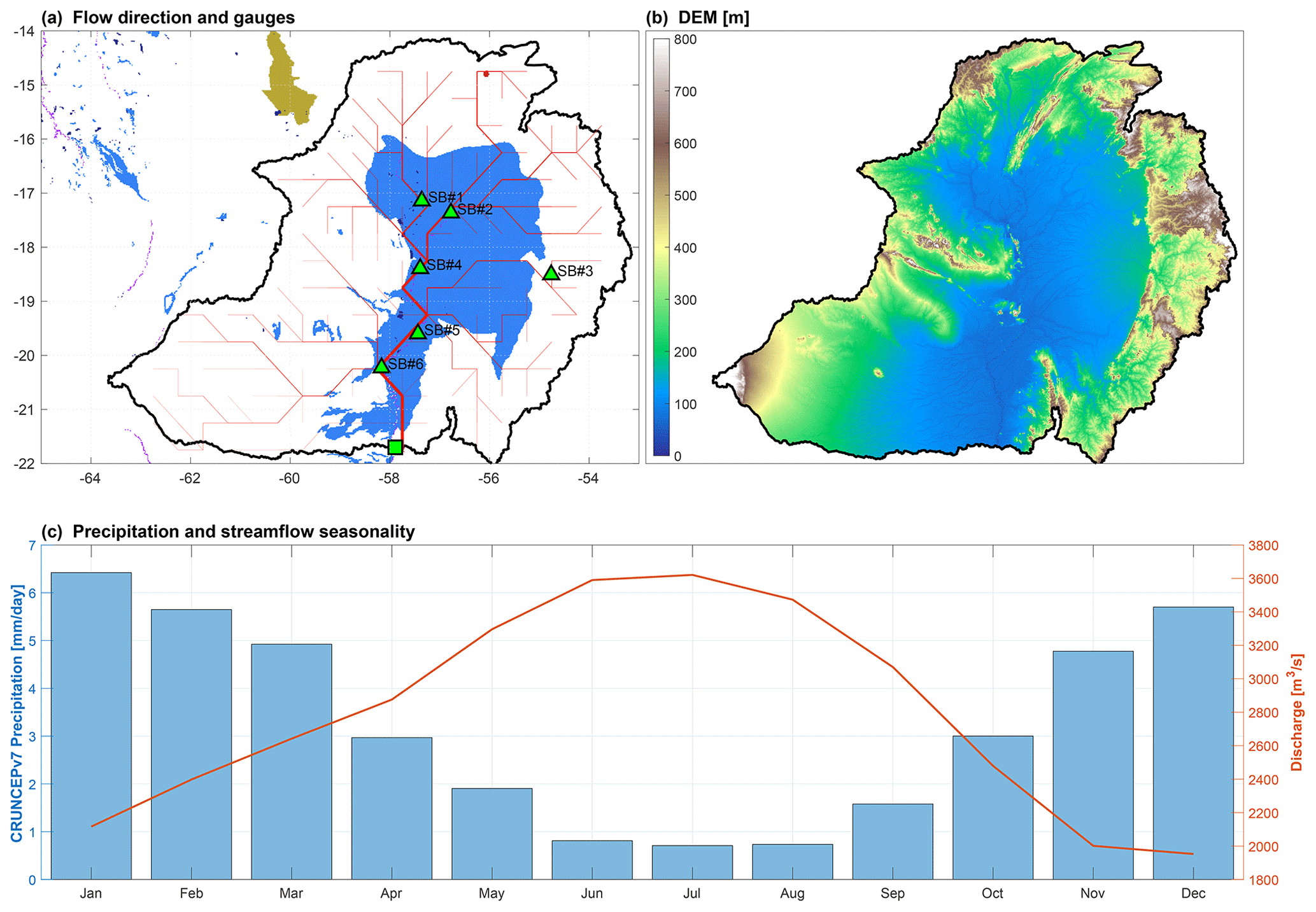
Figure 1 (a) Study domain of the upper Paraguay basin. The red line shows the river network, and the green square denotes the streamflow outlet (i.e., station Porto Murtinho) used in this study. The green triangles are the subbasin (SB) gauges that were used for evaluation. The blue area represents the floodplain according to the Global Lakes and Wetlands Database of Lehner and Döll (2004). (b) DEM at 90 m resolution from Hydrological Data and Maps Based on Shuttle Elevation Derivatives at Multiple Scales (HydroSHEDS; Lehner et al., 2008). (c) Precipitation seasonality derived from CRUNCEPv7 (bar plot relies on left y axis) and observed streamflow seasonality from the outlet of the upper Paraguay basin (solid red line relies on right y axis) during 1979–2009.

2.3 Model setup

We ran one-way coupled ELM–MOSART (i.e., runoff simulated by ELM is send to MOSART for routing) simulations at a spatial resolution of 0.5^∘ × 0.5^∘ for 1979–2009. The simulations were forced by CRUNCEPv7 atmosphere forcing in this study, since it was found to be most accurate over the Pantanal region (Schrapffer et al., 2020). CRUNCEPv7 is a 6-hourly 0.5^∘ × 0.5^∘ global forcing dataset that was generated based on Climatic Research Unit Time-Series Version 3.24 (CRU TS v3.24; Harris et al., 2014) and NCEP reanalysis (Kalnay et al., 1996). The time step for ELM and MOSART is 30 and 60 min, respectively, with a coupling frequency of 180 min.

We performed nine experiments as listed in Table 1 to investigate the sensitivity of streamflow to different processes. The first experiment is the control simulation, using the default ELM surface data and parameters and the default MOSART parameters. In experiment 2, floodplain inundation was turned on to show the impact of floodplain water storage on the streamflow seasonality. Experiment 3 tested the uncertainty of river geometry, and experiment 4 tested the uncertainty of main-channel Manning coefficient (n_r). In experiment 5, we perturb the decay factor for the subsurface runoff generation (f_drai), which has been identified as the most sensitive parameter for subsurface water dynamics (Huang et al., 2013; Bisht et al., 2018). In experiment 6, we aim to understand how streamflow is affected by wetland inundation processes, for which f_over and f_c are critical parameters (see Sect. S1). Experiment 7 represents the calibration of river routing processing, including both geometry and Manning coefficient as uncertain. Experiment 8 calibrates both subsurface and surface water dynamics processes in the runoff generation process. Lastly, experiment 9 is the proposed two-step calibration with all the parameters from experiments 3–6 included (details can be found in Sect. 2.5). We used the diffusion wave routing in MOSART for all the experiments to include backwater effects.

River geometry is assumed to be rectangular (Fig. 1a of Luo et al., 2017), and the main-channel bankfull width (w) and depth (d) can be derived with the equations proposed by Andreadis et al. (2013):

$$\begin{array}{}\text{(1)}& {\displaystyle }w=a_w{Q}^{\mathrm{0.5}},\text{(2)}& {\displaystyle }d=a_d{Q}^{\mathrm{0.3}},\end{array}$$

where Q is the 2-year return period daily streamflow, which is estimated at each grid cell by aggregating daily runoff of the Global Reach-level Flood Reanalysis dataset (GRFR; Yang et al., 2021) from the corresponding upstream area, and a_w and a_d are curve-fitting parameters. Andreadis et al. (2013) found the 95 % confidence intervals for a_w and a_d are [2.6, 20.2] and [0.12,0.63], respectively. Subsurface runoff (R_drai) is parameterized as the exponential function of f_drai and water table depth (z_∇):

$$\begin{array}{}\text{(3)}& R_{\mathrm{drai}}=q_{\mathrm{drai},\max }\exp \left(-f_{\mathrm{drai}}{z}_{\mathrm{\nabla }}\right),\end{array}$$

where q_drai,max is the maximum drainage rate. A surface water storage (i.e., depression areas where excess runoff accumulates) (Ekici et al., 2019) was introduced in ELM to simulate wetlands and subgrid waterbodies, and details can be found in Sect. S1 of the Supplement. A modified wetland scheme of Xu et al. (2023a) is adopted here to improve the wetland inundation simulation (see details in Sect. S1), and two parameters were found to be sensitive for the wetland inundation: f_over and f_c.

In summary, a_w, a_d, and n_r are the parameters in MOSART, and experiments 2, 3, 4, and 7 are hydraulic sensitivity experiments. f_drai, f_over, and f_c are the parameters in ELM, and experiments 5, 6, and 8 are hydrology sensitivity experiments.

Table 1 Simulation experiment designs.

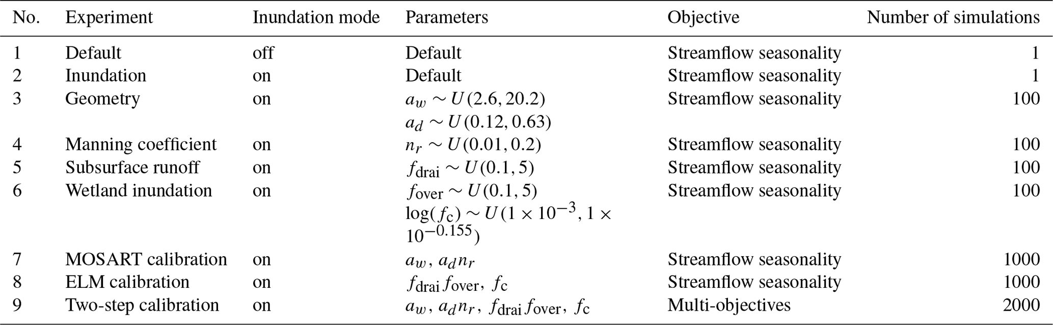
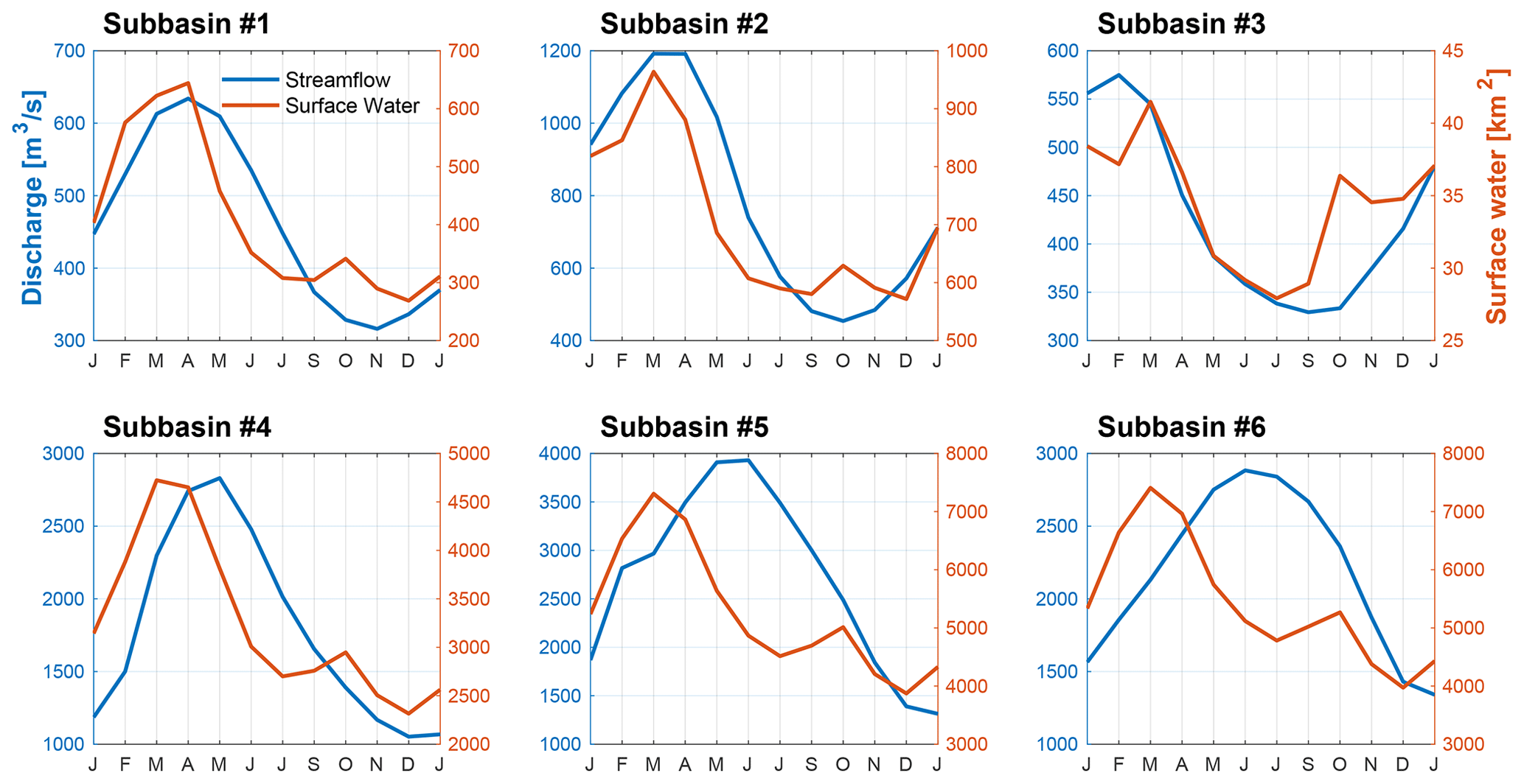
Figure 2 Streamflow seasonality derived from GSIM observations during 1979–2009 (solid blue line) and seasonality of surface water dynamics from GLAD dataset (solid red line) at subbasins in the Pantanal region.

2.4 Data

Multiple datasets of site observations, satellite observations, and reanalysis products were used in this study for model calibration and evaluation. The simulated streamflow was validated at monthly and annual timescales. We used monthly streamflow observations at the Porto Murtinho gauge station (basin outlet shown in Fig. 1a) and six internal subbasin gauges (Fig. 1a) that are archived in Global Stream Indices and Metadata (GSIM; Do et al., 2018; Gudmundsson et al., 2018). The three global runoff datasets that were used to benchmark the performance of annual streamflow include Global Runoff Reconstruction (GRUN; Ghiggi et al., 2019), Linear Optimal Runoff Aggregate (LORA; Hobeichi et al., 2019), and Global Reach-level Flood Reanalysis (GRFR; Yang et al., 2021). The global surface water dynamics dataset from Global Land Analysis and Discovery (GLAD; Pickens et al., 2020) was used to validate the simulated surface water fraction (SWF), which is the sum of ELM-simulated inundation and MOSART-simulated inundation in E3SM (Xu et al., 2023a). GLAD provides global monthly, annual, and seasonal surface water and permanent water layer derived from Landsat images during 1999–2020 at 0.00025^∘ × 0.00025^∘ (∼30 m × 30 m) resolution. We used seasonal GLAD and removed the permanent water to exclude the rivers and lakes from the SWF. The GLAD was upscaled to 0.5^∘ × 0.5^∘ by averaging the values from all the finer-resolution grid cells within the coarse-resolution grid cell to compare with the model simulations. The gridded energy flux data (FLUXCOM; Jung et al., 2019) and Global Land Evaporation Amsterdam Model version 3 (GLEAMv3; Martens et al., 2017) product were used to evaluate evapotranspiration (ET).

2.5 Calibration procedure

We propose a two-step calibration procedure in this study to appropriately resolve hydrological and hydraulic impacts on streamflow variability. In step 1, we run 1000 simulations with runoff-generation-related parameters (f_drain, f_over, and f_c) randomly sampled from the prior distributions given by experiment 8 in Table 1. A multi-objective function was proposed by Yang et al. (2019) to calibrate a land surface model, which is adopted in this study. The best parameter was calibrated in each individual grid cell to minimize the following objective function (obj) to capture SWF, baseflow index (BFI), and annual streamflow trend (Trend) simultaneously:

$$\begin{array}{}\text{(4)}& \begin{array}{rl}\text{obj}& =w_{\mathrm{1}}\cdot \left|\log \left({\displaystyle \frac{{\mathrm{SWF}}_{\mathrm{sim}}}{{\mathrm{SWF}}_{\mathrm{glad}}}}\right)\right|+w_{\mathrm{2}}\cdot \left|\log \left({\displaystyle \frac{{\mathrm{BFI}}_{\mathrm{sim}}}{{\mathrm{BFI}}_{\mathrm{GSCD}}}}\right)\right|\\ & +w_{\mathrm{3}}\cdot \left|\log \left({\displaystyle \frac{{\mathrm{Trend}}_{\mathrm{sim}}}{{\mathrm{Trend}}_{\mathrm{obs}}}}\right)\right|,\end{array}\end{array}$$

where SWF_sim represents annual averaged simulated surface water fraction from the coupled ELM–MOSART simulations, and SWF_glad is the GLAD annual averaged surface water fraction. SWF was estimated between 1999–2009, when the simulation period overlapped with GLAD temporal availability. We note the simulated SWF includes both ELM-simulated and MOSART-simulated inundation. But only the ELM-relevant parameters were calibrated to optimize Eq. (4), as routing process is not considered in the step-1 calibration. Therefore, the SWF in the objective function Eq. (4) is only affected by ELM processes. BFI_sim and BFI_GSCD are the baseflow index (i.e., the ratio of subsurface runoff to total runoff) from simulations and the Global Streamflow Characteristics Dataset (GSCD; Beck et al., 2013), respectively. “Trend” denotes the trend of annual runoff quantified by Sen's slope (Sen, 1968). Because there is no reliable gridded dataset of the long-term runoff trend, we assumed Trend_obs to be constant over the whole basin, and the value was derived from observed streamflow at the outlet. This assumption may introduce uncertainty in the model for capturing the heterogeneity of runoff sensitivity to climate change. Although several internal subbasin gauges exist, their temporal coverages are shorter than the simulation period, so they cannot be used to derive annual runoff trends within the watershed. Due to the different bias magnitudes and uncertainty patterns, the assignment of weights is subjective (Yang et al., 2019). In step 2, another 1000 simulations were performed with river routing parameters (a_w, a_d, and n_r) randomly sampled from the uniform distribution in Table 1 and the calibrated hydrological parameters from step 1. The best a_w, a_d, and n_r were calibrated at basin level by maximizing the correlation coefficient between monthly simulated and observed streamflow at the outlet. As suggested by Shen et al. (2022), we used all the streamflow observations for calibration without splitting the validation period. We further validate the calibrated model at six internal subbasin gauges (Fig. 1a), which are not used during the calibration process.

3 Results and discussion

3.1 Streamflow variability in the Pantanal region

Figure 2 illustrates the observed streamflow seasonality from six selected subbasins in the Pantanal region, with the streamflow peaks shifting from March in the headwater (subbasins 1, 2, and 3) to June downstream of the river (subbasin 6). Streamflow variability reflects the combined effects of routing surface runoff and subsurface runoff. Surface runoff is closely related to the surface water dynamics, which are controlled by the hydraulic factor, such as floodplain inundation processes. However, the surface water dynamics have a much earlier seasonality (i.e., peak in March) than the streamflow at the downstream gauges (subbasins 4, 5, and 6). The differences in the seasonality between surface water dynamics and outlet streamflow imply the significant contribution of subsurface runoff to the streamflow variability. The subsurface runoff generation is the hydrological process, simulated by a land surface model (e.g., ELM). Therefore, both hydrological and hydraulic processes have impacts on the significant shift in the seasonality between precipitation and streamflow in the Pantanal region.

3.2 Impacts of MOSART on streamflow variability

The default coupled ELM–MOSART simulation (i.e., experiment 1) fails to capture the streamflow seasonality over the Pantanal region. Specifically, the default simulation shows streamflow peaks around March, which is much earlier than the observed streamflow peaks in July (Fig. 3). Previous studies found that the late responses of streamflow peaks to precipitation are caused by the storage effects of the floodplain (Schrapffer et al., 2020). However, in our inundation experiment (i.e., experiment 2), turning on the inundation mode only delays the streamflow seasonality by 1 month compared to the default configuration, which still cannot capture the observed seasonality well (Fig. 3). This discrepancy suggests significant uncertainties exist in other river-routing-related or runoff-generation-related parameters. For example, our geometry experiment (i.e., experiment 3) demonstrates that smaller a_w and a_d lead to a higher model performance of capturing streamflow seasonality, such as a higher correlation coefficient of monthly streamflow between the simulations and observations (Fig. 4a). Smaller a_w and a_d (i.e., smaller cross-section area) correspond to less channel capacity, implying that more water will inundate on the floodplain during the flooding period; therefore, the peak streamflow is delayed to a later time. Although the streamflow seasonality is improved by reducing channel cross-section area, it results in smaller temporal variations in monthly streamflow, such as the ratio of standard deviation (rSD) between the simulations and observations being less than 0.85. The smaller rSD indicates the regulation of the floodplain is magnified; therefore, it is not reasonable to accept such small channel geometry.

Figure 3 Simulated streamflow seasonality of default simulation (experiment 1 in Table 1) and default simulation with inundation mode (experiment 2 in Table 1). The seasonality is derived from 1979 to 2009.

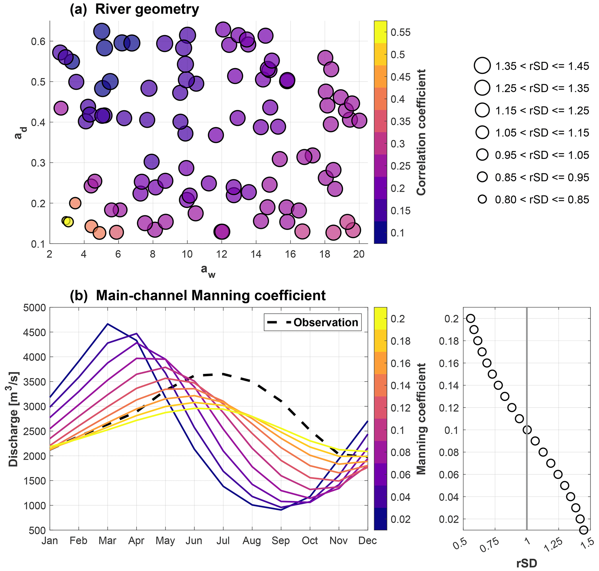
Figure 4 Sensitivity of streamflow seasonality and variability to (a) river geometry and (b) main-channel Manning coefficient. In (a), a_w and a_d are the parameters for river width and depth, respectively (Eqs. 1 and 2), and the correlation coefficient between the simulated streamflow and observed streamflow at monthly scale is used to indicate the model performance of simulating streamflow seasonality. The scatter size is proportional to the ratio of standard deviation (rSD) between the simulated streamflow and observations. The dashed black line in (b) represents the averaged streamflow seasonality derived from observations, and the scatter on the right shows the relationship between the main-channel manning coefficient (y axis) and rSD (x axis).

The Manning coefficient of the main channel affects the streamflow seasonality through its impacts on flow velocity. In the Manning coefficient experiment (i.e., experiment 4), increasing the main-channel Manning coefficient will at most shift the occurrence of peak streamflow to June (Fig. 4b), while the corresponding value (nr≥0.16) is much higher than the generally used main-channel Manning coefficient in global river transport models (e.g., 0.03–0.06; Yamazaki et al., 2011; Li et al., 2013; Decharme et al., 2012). A larger Manning coefficient means slower flow velocity along the river direction, and then the water will accumulate in the channel and inundate the floodplain when it exceeds the channel capacity. Notably, such high main-channel Manning coefficients lead to an unrealistic flatter hydrograph with rSD <0.7. Using a Manning coefficient at around 0.1 reproduces the monthly variability best (e.g., rSD = 1), which is still higher than the typical value, but such a range may be reasonable in this region because of the vegetated surface and complex river network (i.e., meandering) according to Chow (1959). The subnetwork and hillslope manning coefficients in MOSART are not included in our experiments because they have negligible impacts on the shape of the hydrograph (Fig. S4).

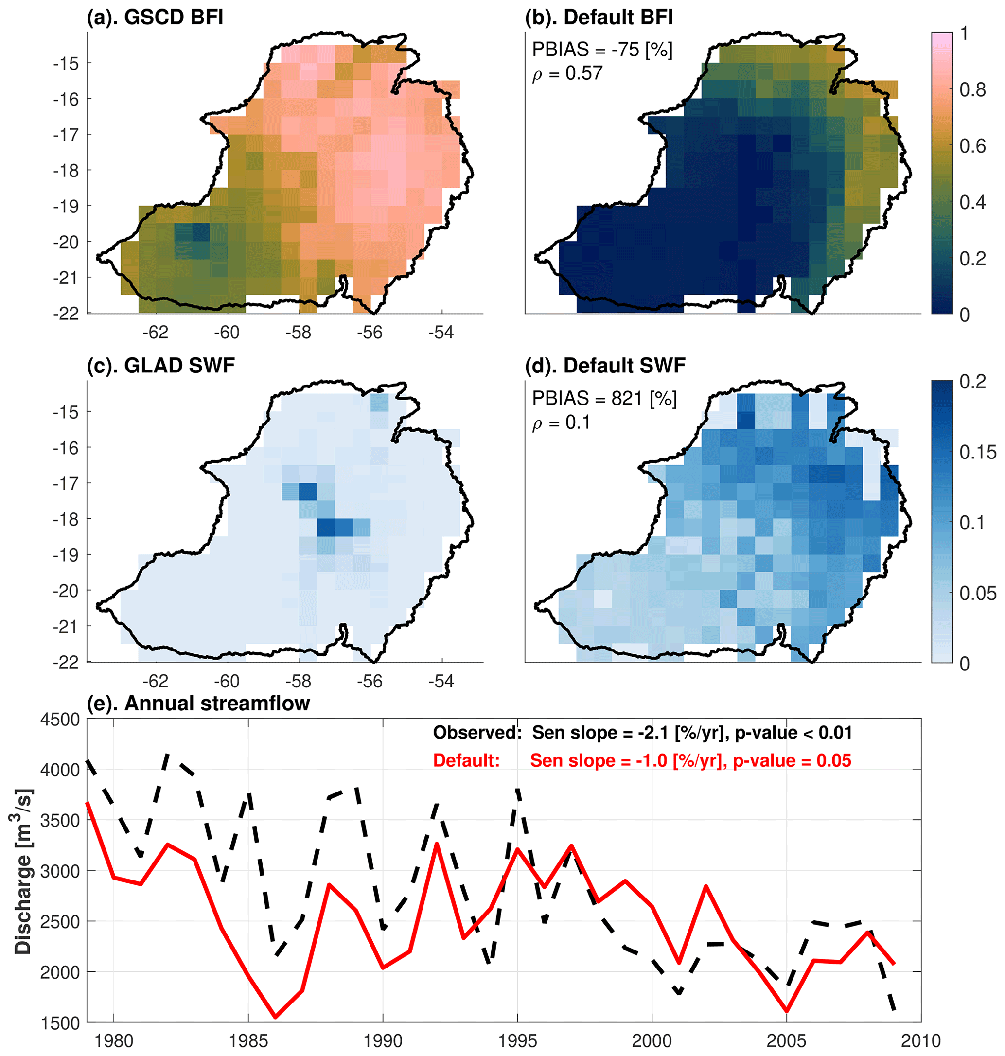
Figure 5 Performance of ELM–MOSART with default configuration. (a) Base flow index (BFI) from GSCD BFI3, (b) simulated BFI with default parameter, (c) surface water fraction (SWF) from GLAD, (d) simulated SWF (floodplain inundation plus wetland inundation) with default parameter, and (e) annual streamflow time series of observations (dashed black line) and default simulation (solid red line) at basin outlet.

Although calibrating channel geometry and Manning coefficient improves the performance of the coupled ELM–MOSART model in simulating streamflow, some discrepancies in the streamflow seasonality and variation between the simulations and observations exist. Floodplain effects cannot completely explain the streamflow seasonality in the Pantanal region. Additionally, other variables in the water cycle remain highly biased, which cannot be fixed by calibrating river-routing-related parameters. First, the simulated BFI averaged over the basin is about 0.15, which significantly underestimates the values (e.g., 0.69) estimated by the Global Streamflow Characteristics Dataset (GSCD; Beck et al., 2013) (Fig. 5a and b). Second, the surface water dynamics are poorly simulated with a low spatial correlation coefficient (0.03) and high percentage bias (821 %) as compared to the upscaled GLAD dataset (Fig. 5c and d). Third, the Pantanal region has become drier in the past several decades (Libonati et al., 2020), which can be detected from the observed annual streamflow time series (Fig. 5e). While the model is able to capture the drier trend of annual streamflow during the simulation period (negative Sen's slope with p value = 0.05), the magnitude of the decreasing trend is underestimated (Fig. 5e). The above discrepancies can be reduced by calibrating the runoff-generation-related processes (e.g., hydrological control) because the river routing process only impacts the shape of the hydrograph.

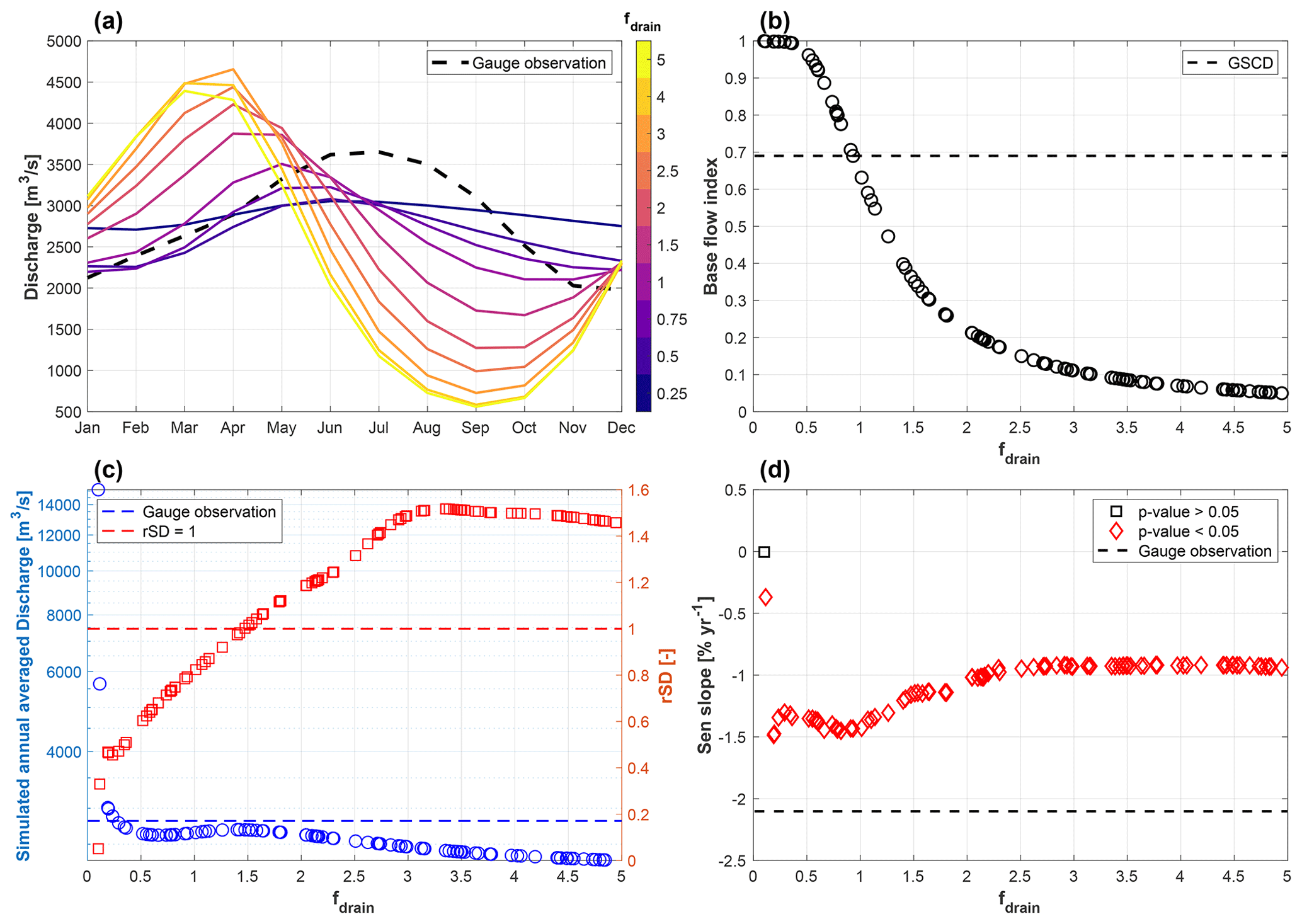
Figure 6 Sensitivity of (a) streamflow seasonality, (b) base flow index, (c) annual streamflow mean and rSD, and (d) annual streamflow trend to f_drain. rSD denotes the ratio of monthly standard deviation between the simulations and observations. Note that Sen's slope is normalized by the annual averaged streamflow.

3.3 Impacts of ELM on streamflow variability

The subsurface runoff experiment (i.e., experiment 5) demonstrates the subsurface runoff generation process has a critical control on the streamflow seasonality as well (Fig. 6). It is shown in Fig. 6a that the simulated streamflow tends to peak later as f_drain decreases. A decrease in f_drain means the subsurface storage capacity increases (Huang et al., 2013), therefore leading to a higher base flow index (Fig. 6b). This explains the response of total runoff to rainfall being delayed when smaller f_drain was used due to the slower mechanism of subsurface runoff (Vivoni et al., 2007). Furthermore, smaller f_drain leads to increased annual streamflow magnitude but reduced monthly streamflow variability (Fig. 6c). We acknowledge unrealistically high streamflows (e.g., mean >5000 m³ s⁻¹) with minimal month-to-month variability (e.g., rSD <0.4) are found in the simulations when f_drain is close to 0.1; thus a more reasonable lower bound of $f_{\mathrm{drain}}^{\prime }s$ should be modified to a relatively larger value (e.g., 0.25). Moreover, the trend of annual simulated streamflow can be affected by f_drain, though all the simulations tend to underestimate the trend detected in the observations. The decreasing trend is more significant and closer to the observed trend when f_drain decreases (Fig. 6d), except two problematic simulations with very small f_drain.

The sensitivity of the annual runoff trend (i.e., annual streamflow trend) to f_drain results from the impacts of f_drain on ET processes. As a conceptual example, the runoff will not have a trend in time if precipitation and ET have similar decreasing trends (e.g., P and E₁ in Fig. 7a). Runoff will show a trend in time when the changing rate of ET is different from precipitation (e.g., P and E₂ in Fig. 7a). The subsurface runoff experiment shows that the ET is less sensitive to precipitation decreases with smaller f_drain (Fig. 7b), thus leading to a larger decreasing trend in annual runoff (light green line in Fig. 7a). Based on the above analyses, it is reasonable to argue that a good selection of f_drain in this region should be smaller than the default value (i.e., 2.5), which will yield later streamflow seasonality and better estimates of base flow index, monthly variability, and the annual trend compared to reference data or observations.

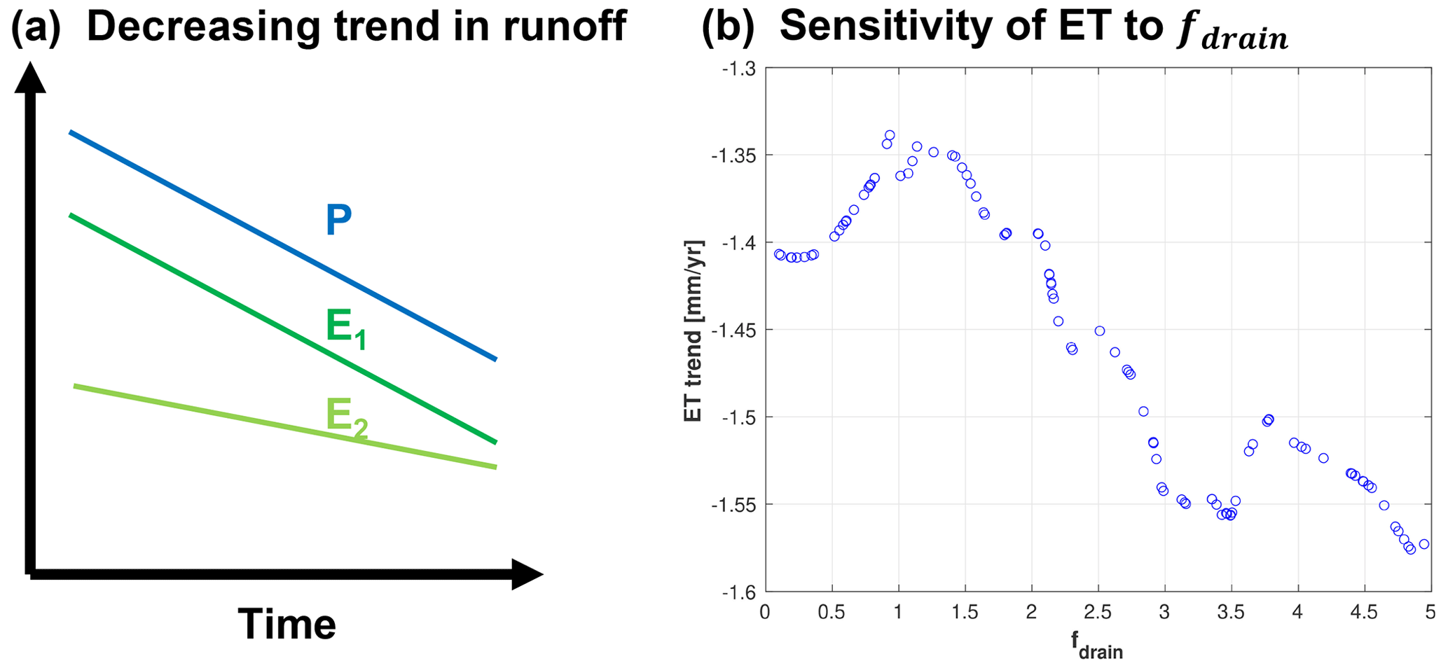
Figure 7 (a) Conceptual plot of annual precipitation (P) and two different annual evapotranspiration time series (i.e., E₁ and E₂), with the decreasing trend of E₁ being larger than that of E₂. Panel (b) shows the sensitivity of annual ET trend (e.g., Sen's slope of annual basin-averaged ET during the simulation period) to f_drain.

Parameters f_over and f_c control the streamflow variability through wetland inundation processes based on our wetland inundation experiment (i.e., experiment 6) (Fig. 8a) and previous study (Xu et al., 2023a). Wetland inundation is only sensitive to f_c when f_over is smaller than 0.5, as small f_over leads to a higher saturated fraction, at which infiltration from the wetlands is constrained and inundation occurs (Fig. S3a). In contrast to the impacts of floodplain inundation, higher wetland inundation is associated with earlier streamflow peaks (Fig. 8b). This is because high wetland inundation is caused by precipitation when the saturation fraction is high (e.g., lower f_over); consequently, a larger fraction of precipitation is converted to surface runoff. Hence, the streamflow seasonality is very close to precipitation seasonality when high wetland inundation is simulated, since surface runoff responds quickly to precipitation. The annual streamflow magnitude and trend are also sensitive to the wetland inundation processes (Fig. 8c and d), especially when parameter f_over falls in the lower range (e.g., less than 1.5). Specifically, the annual streamflow magnitude increases, and the trend becomes less negative as f_over decreases.

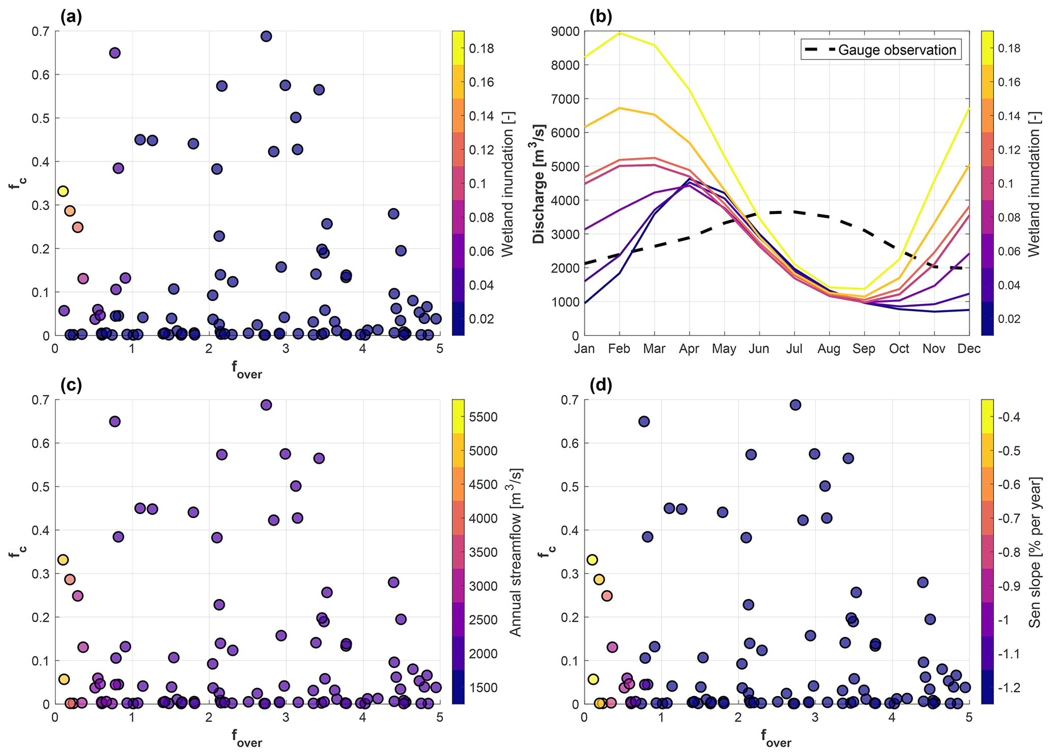
Figure 8 (a) Sensitivity of wetland inundation to f_c and f_over. (b) Impacts of wetland inundation on streamflow seasonality. Sensitivity of (c) annual streamflow and (d) annual streamflow trend to f_c and f_over. Note that Sen's slope is normalized by the annual averaged streamflow.

3.4 Single-process calibration

We further conducted two independent calibrations for both the river routing process in MOSART and the runoff generation process in ELM using experiments 7 and 8 (Table 1), respectively. Specifically, the objectives of both independent calibrations are to maximize the correlation coefficient between the simulated and observed streamflow time series. Both calibrations can improve the streamflow seasonality significantly as compared to the default configuration, with correlation coefficients increasing from 0.02 to 0.75 and 0.67, respectively (Fig. 9a and b). The long-term averaged annual streamflow remains similar in the default configuration and two calibrations, with all underestimating the observations by about 10 %. However, the temporal variations in simulated streamflow time series in the two calibrations show divergent bias patterns, with the MOSART calibration resulting in a smaller standard deviation (e.g., rSD = 0.74) and the ELM calibration leading to a slightly higher standard deviation (e.g., rSD = 1.06) (Fig. 9b).

The individual MOSART calibration can lead to a very high Manning coefficient (e.g., nr=0.17) and a smaller cross-section of the main channel to capture the streamflow seasonality. Consequently, the flow velocity is slower, and more river water inundates the floodplain due to backwater effects, which results in a significant underestimation in the temporal variation in simulated streamflow (Fig. 9b). The individual ELM calibration leads to an unreasonably higher baseflow index (Fig. 9b), implying the subsurface and surface water dynamics are not well represented. Overall, only calibrating the parameters related to one process results in unrealistic parameter values to compensate the bias from the other process. Therefore, the impacts of both runoff generation and river routing processes on streamflow must be considered together in calibrating the streamflow simulation to ensure all the processes of the water cycle are well calibrated.

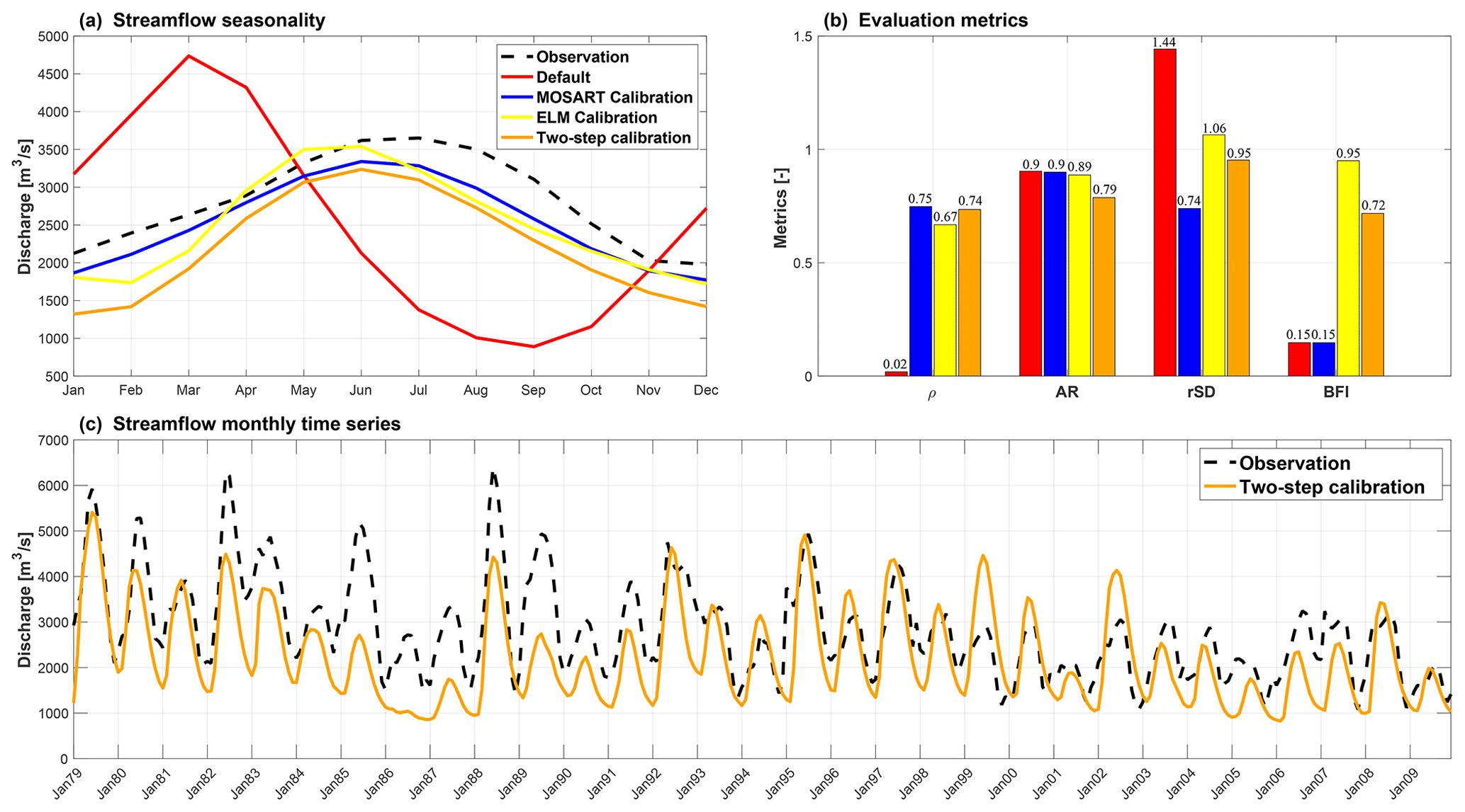
Figure 9 Comparison of hydraulic, hydrological, and two-step calibrations with the default configuration. Panel (a) shows the seasonality from the simulation period, and panel (b) denotes the correlation coefficient (ρ), annual streamflow ratio (AR), ratio of standard deviation between the simulations and observations (rSD), and baseflow index (BFI). Panel (c) presents the monthly time series of simulated streamflow after the two-step calibration.

3.5 Two-step calibration

We propose a two-step calibration procedure in this study (Sect. 2.5) by first calibrating the runoff-generation-relevant parameters in ELM and then calibrating the river-routing-relevant parameters in MOSART. Since it is unclear how much the streamflow delay is attributed to the runoff generation process, we use other objectives (i.e., independent of streamflow variability) in the ELM calibration (Eq. 4). It is implied from the analyses of runoff-related parameters that the runoff seasonality is related to the objectives used in Eq. (4). Therefore, we assume the delay of streamflow attributed to the runoff generation process can be addressed by minimizing Eq. (4). In the multi-objective function, we found w₁=0.15, w₂=0.7, and w₃=0.15 yield the best results. The calibrated simulation shows good skill in capturing the spatial pattern of baseflow index and surface water fraction with correlation coefficients of 0.7, and 0.64, respectively, as compared to the reference data (Fig. 10a and b). The absolute biases are significantly reduced as well. Moreover, the calibrated simulation shows a statistically significant decreasing trend in the annual streamflow with Sen's slope equal to −1.80 % yr⁻¹ after normalizing with averaged annual streamflow magnitude. As a benchmark, we found other calibrated or bias-corrected runoff datasets cannot capture either the annual magnitude or annual trend (Fig. 10c). The uncertainty of the annual magnitude may stem from the forcing uncertainty, while the trend bias is because model sensitivity to climate change is not well constrained. This suggests including the trend as a performance metric in the objective function is necessary for calibrating ESMs, which are commonly used to project the change in the water, energy, and carbon cycle under a warmer climate. Although water table depth is not included in the objective function, the simulated water table depth is more consistent with the dataset of Fan et al. (2013) than the default configuration, which simulates a very shallow water table (Fig. S5). The improved representation of groundwater table depth is because the subsurface and surface runoff are correctly separated (e.g., a better-simulated baseflow index).

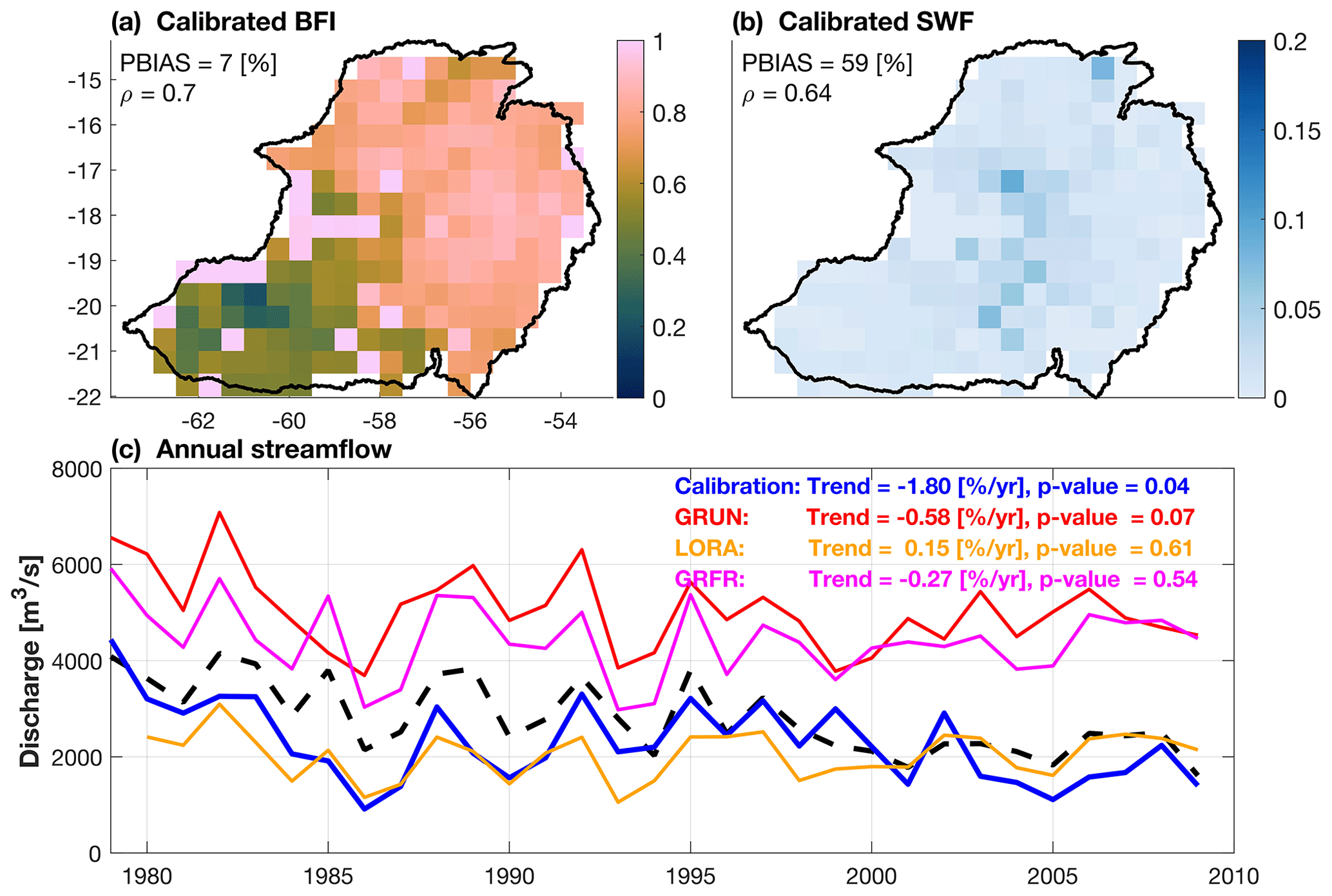
Figure 10 Performance of ELM–MOSART with calibrated ELM parameters for (a) base flow index (BFI), (b) surface water fraction (SWF), and (c) annual streamflow trend. Three other runoff datasets are used to provide benchmarks for annual streamflow. The dashed black line represents the observations from the outlet, with the annual trend (i.e., Sen's slope) being −2.1 % yr⁻¹ and the corresponding p value less than 0.05.

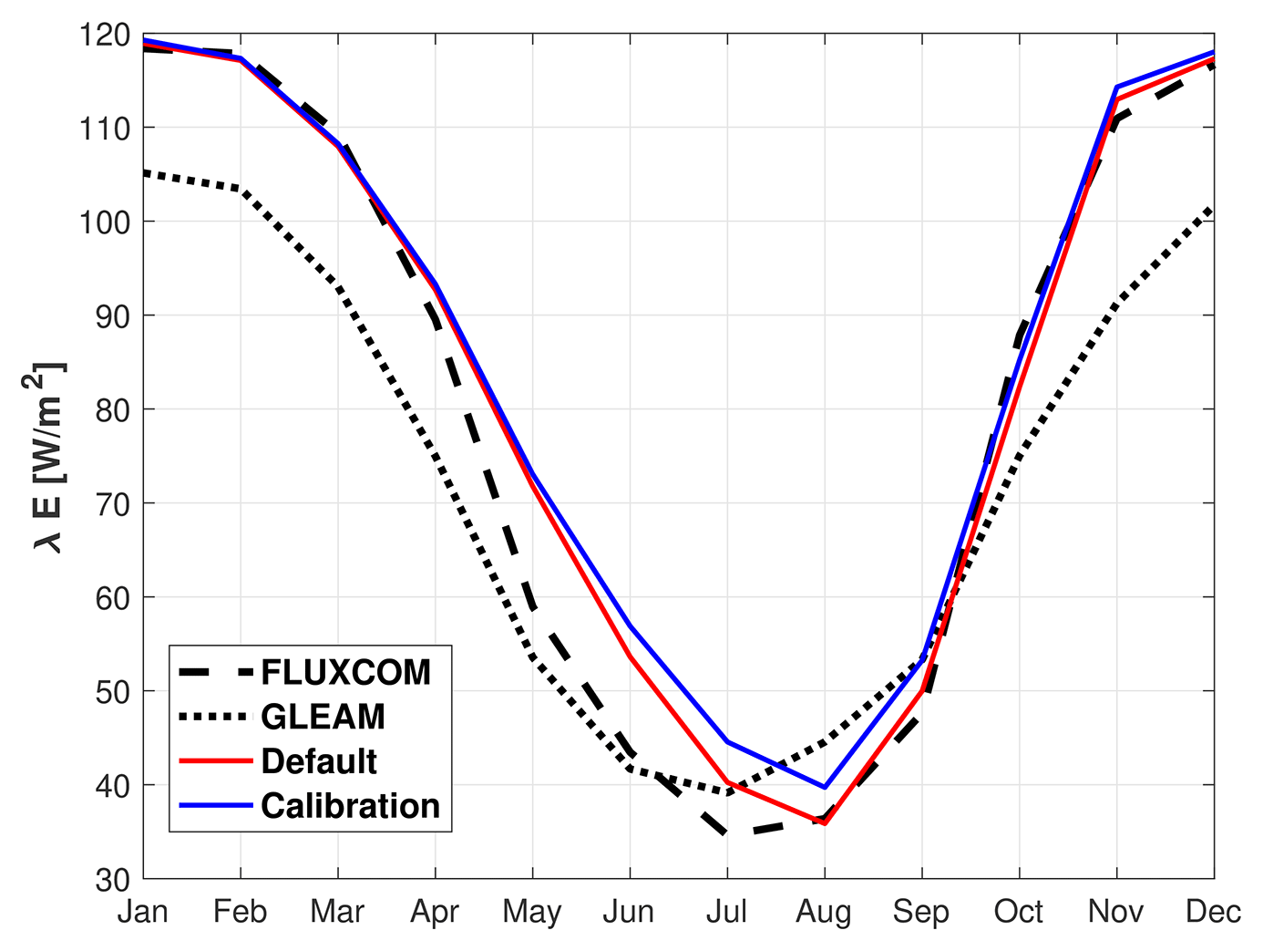
With hydrology parameters determined from the step-1 calibration, the model shows good performance of simulating monthly streamflow after the step-2 calibration (Fig. 9c). Specifically, the correlation coefficient between the simulations and observations at the monthly scale is 0.74, indicating the streamflow seasonality is well captured. Compared to the individual MOSART or ELM calibration, the two-step calibration shows better skill in both monthly variation (e.g., rSD = 0.95) and baseflow index (e.g., BFI = 0.72) (Fig. 9b). However, the two-step calibration exhibits higher biases in the annual streamflow magnitude (e.g., 21 % underestimation or 32 mm yr⁻¹ in absolute magnitude), stemming from the following reasons: (1) uncertainty of upscaled flow directions in MOSART because of the relatively coarse spatial resolution (∼50 km × 50 km) (Liao et al., 2022). For example, the contributing area of the selected outlet estimated using the modeled flow direction underestimates ∼5 % of the contributing area that is delineated with the 1 km Hydrological Data and Maps Based on Shuttle Elevation Derivatives at Multiple Scales (HydroSHEDS) DEM. (2) Another reason is the uncertainty of the forcing data. Specifically, the annual averaged precipitation in CRUNCEPv7 is lower than the mean of multiple precipitation products (Fig. S6a). Considering the selected precipitation ensemble (Table S1), the uncertainty of CRUNCEPv7 precipitation varies between −73–49 mm yr⁻¹. Biases may exist in other forcing variables (e.g., humidity and radiation) as well (Fig. S7), resulting in an overestimation of evapotranspiration during the dry period (e.g., May to July) as compared to FLUXCOM (Fig. 11). For the reference ET of the GLEAM dataset, the simulated ET is higher for all the months. The overestimation of simulated annual averaged ET is 54 and 154 mm yr⁻¹ compared to FLUXCOM and GLEAM, respectively. In addition, Xu et al. (2023b) also reported that the energy partition algorithm in current ESMs tends to overestimate ET likely due to the uncertainty in surface conditions and parameterizations of aerodynamic and stomatal resistance. In summary, while our calibrated model underestimates streamflow magnitude, the result is reasonable as the negative bias is consistent with the smaller contributing area, lower precipitation forcing, and higher evapotranspiration estimates. Furthermore, CRUNCEPv7 shows a notable reduction in precipitation from January to February, while other precipitation products show a similar precipitation volume in January and February (Fig. S6b). The underestimation of precipitation in February further explains the slightly earlier streamflow seasonality after the two-step calibration.

Figure 11 Comparison of latent heat flux between simulations and references.

After the two-step calibration, both the runoff generation and river routing processes are robustly improved in E3SM over the Pantanal region. For example, the objective function of Eq. (4) reduces from 20.8 to 4.1 after the step-1 calibration, and the correlation between the simulated streamflow and observed streamflow at the outlet increases from 0.2 to 0.74 after the step-2 calibration. Although only the observed streamflow at the basin outlet was used during the calibration, the performances of simulated streamflow are improved at selected subbasin gauges compared to the default configuration (Fig. 12). Specifically, compared to the default simulation, the step-1 calibration shifts the streamflow by about 1 month. The step-2 calibration further delays the simulated streamflow seasonality, especially for the downstream subbasins (subbasins 5 and 6). Overall, the calibrated model captures the streamflow monthly variation at all the subbasin gauges well with correlation coefficient larger than 0.6. While the seasonality is well captured, the calibrated model cannot reproduce the magnitude of streamflow well at the headwater subbasins (subbasins 1, 2, and 3) likely due to the uncertainty of precipitation in the forcing and bias of flow direction represented in MOSART (Fig. S8). The relative higher uncertainties in small subbasins are expected in the context of ESMs, as large-scale coupled land–river models are commonly evaluated at major global river basins (Yamazaki et al., 2011; Li et al., 2015; Decharme et al., 2019). We note that the number of simulations in the two-step calibration, such as a total of 2000 simulations, is enough to identify the parameter values that approximate the best parameter values. As shown in Fig. S9, the improvements in model performance reach a plateau when the number of calibration simulations is larger than 200 in both steps.

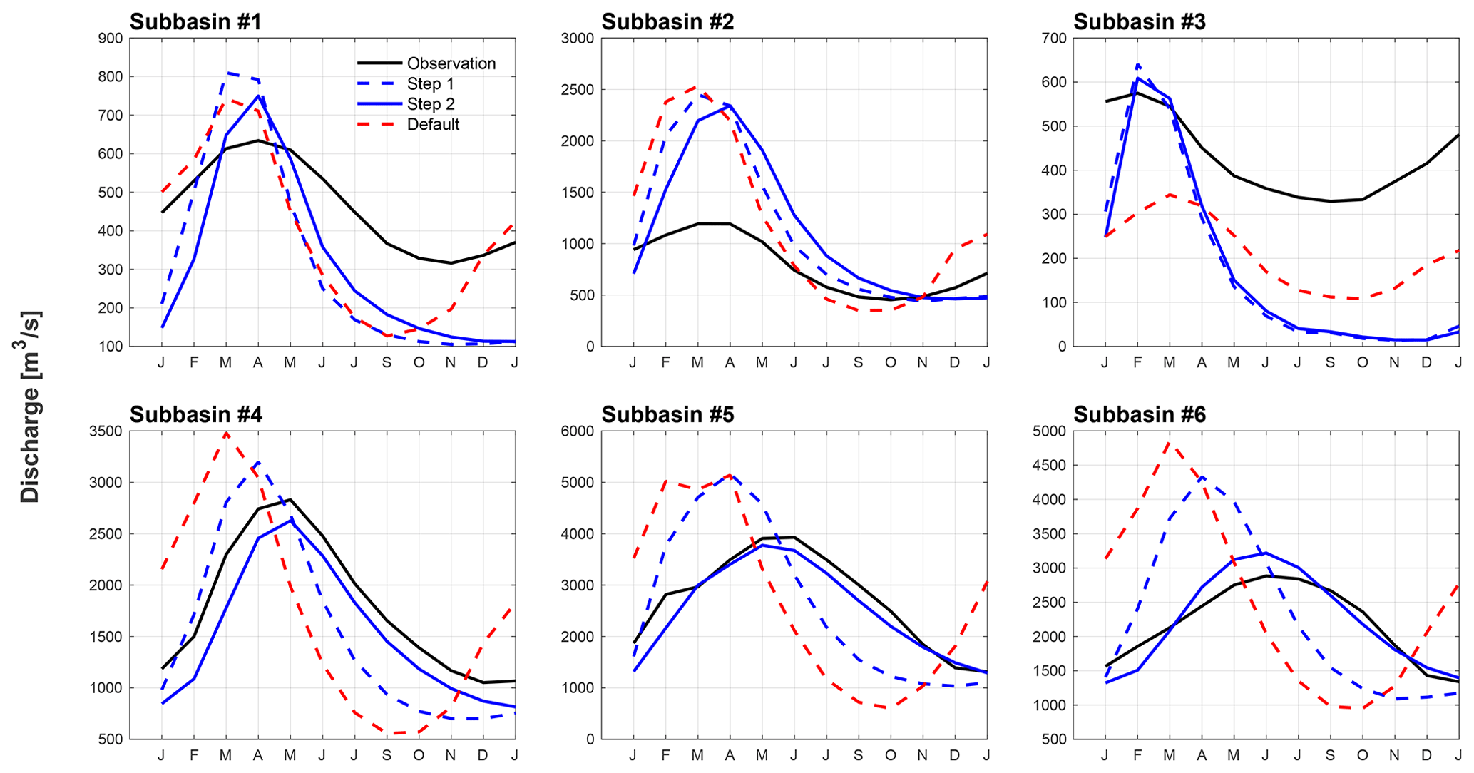
Figure 12 Simulated streamflow seasonality during 1981–2010 for the selected subbasins with default parameter values (dashed red line) and calibrated parameter values after step 1 (dashed blue line) and step 2 (solid blue line). The solid black line denotes the observed streamflow seasonality.

Figure S10 shows the calibrated parameter values, and we note it is hard to identify the relationship between the calibrated parameters and watershed characteristics due to the coarse spatial resolution of ESMs and simplifications in physical processes. As process-based models, some parameters in ELM and MOSART are derived from surface and subsurface conditions and properties. For example, in ELM, saturated hydraulic conductivity and specific yield are estimated based on soil types, maximum drainage rate is determined by topographic slope, etc. In MOSART, river length and slope are derived from a high-resolution DEM. However, some other parameters should be determined based on sensitivity analysis and calibration, such as the parameters selected in this study. This is because ESM resolutions are typically too coarse to represent some small-scale physical processes, and empirical functions are used to parameterize those processes with simplifications. Specifically, f_drain and f_over are decay factors of the exponential function in the subsurface and surface runoff generation processes, respectively. According to the development of the runoff scheme in our model (e.g., simple TOPMODEL-based runoff parameterization), f_drain and f_over should be determined through sensitivity analysis or calibration against a hydrograph recession curve (Niu et al., 2007, 2005). f_c is a threshold below which no single connected inundated area spans the grid cell. It is used to quantify the fraction of the inundated portion of the grid cell that is interconnected according to percolation theory. In other words, f_c determines the maximum inundation extent, above which the water will drain from the inundated area. Although the maximum inundated area should be controlled by topographic variation, high-resolution data that capture the topographic variation under the inundated areas are not available. Observations of river width and depth exist at very high spatial resolution, but it is challenging to upscale the observed river width and depth to ESM resolution (e.g., ∼1^∘) (Liao et al., 2022). The relationship between discharge (or drainage area) and river channel geometry is commonly used to determine the river width and depth in global river transport models (Xu et al., 2022b; Decharme et al., 2012). However, such a relationship varies from watershed to watershed. It is not possible to use a single factor to derive the river geometry as it is affected by multiple factors such as discharge magnitude, seasonality, lithology, and channel slope.

To assess the transferability and robustness of our approach, we implemented the two-step calibration procedure in a watershed located in a distinct climate and biome, specifically the Susquehanna River Basin. Figure S11 shows that the performance of simulating BFI, SWF, and streamflow seasonality is improved after the calibration with the proposed method.

4 Conclusion

In this study, we investigated the impacts of the runoff generation process and river routing process on streamflow variability in the coupled land and river configuration of E3SM using the Pantanal region as a case study. Previous studies argued that floodplain storage effects are critical in capturing streamflow seasonality in global river transport models (Schrapffer et al., 2020; Yamazaki et al., 2011; Decharme et al., 2012), but we found that the impacts of the runoff generation process on the streamflow variability should not be ignored. Calibrating either the runoff-generation-relevant or river-routing-relevant parameters can improve the performance of simulated streamflow variability, but the system as a whole is not well captured, as the baseflow index, sensitivity of streamflow to climate change, water table depth, and surface water dynamics remain highly biased. This implies that only calibrating one of the two processes results in overfitting and problematic parameter values; i.e., the impact of one process compensates for the bias resulting from the other process. Consequently, such a calibration causes the unrealistic simulation of other relevant variables. Therefore, a two-step calibration procedure is proposed for large-scale coupled land–river simulations to reconcile their impacts on streamflow variability. Specifically, the first step is to calibrate the hydrological parameters at the grid cell level with multiple selected objectives, followed by the second step to calibrate the river model at the basin level in terms of streamflow performance. The two-step calibration exhibits robust performance in the water cycle simulation. The sensitivity of streamflow to climate change was improved as well in our two-step calibration, suggesting the importance of including the annual runoff trend in the hydrological parameter calibration, since trend analysis is of particular interest in earth system modeling. The two-step calibration method demonstrates robust performance in calibrating the E3SM coupled land–river configuration at a watershed with a different climatology and biome.

Although we validated our two-step calibration method in an independent watershed (i.e., Susquehanna River Basin), it remains unclear if it can improve the model performance in other watersheds with different characteristics and climatology. Additional evaluations and careful analysis are needed to apply the proposed calibration method to E3SM or other large-scale hydrological models at global scales. Furthermore, other challenges exist for the global calibration. First, streamflow observations are needed in the two-step calibration, but many watersheds at global scales are not gauged. Machine learning methods can be used to derive benchmark streamflow for the ungauged watersheds (Kratzert et al., 2019). Second, it is computationally expensive or even infeasible to run 2000 global simulations for calibration. However, as demonstrated in Fig. S9, a much smaller number of calibration simulations are needed to find approximately good parameter values. In conclusion, while different objective functions can be used in other model calibrations, we suggest that both runoff generation and river routing processes should be carefully considered together to improve streamflow simulations with coupled land–river models.