Constraining the carbon cycle in JULES-ES-1.0

Land surface models are an important tool in the study of climate change and its impacts, but their use can be hampered by uncertainties in input parameter settings and by errors in the models. We apply uncertainty quantification (UQ) techniques to constrain the input parameter space and corresponding historical simulations of JULES-ES-1.0 (Joint UK Land Environment Simulator Earth System), the land surface component of the UK Earth System Model, UKESM1.0. We use an ensemble of historical simulations of the land surface model to rule out ensemble members and corresponding input parameter settings that do not match modern observations of the land surface and carbon cycle. As JULES-ES-1.0 is computationally expensive, we use a cheap statistical proxy termed an emulator, trained on the ensemble of model runs, to rule out parts of the parameter space where the simulator has not yet been run. We use history matching, an iterated approach to constraining JULES-ES-1.0, running an initial ensemble and training the emulator, before choosing a second wave of ensemble members consistent with historical land surface observations. We successfully rule out 88 % of the initial input parameter space as being statistically inconsistent with observed land surface behaviour. The result is a set of historical simulations and a constrained input space that are statistically consistent with observations. Furthermore, we use sensitivity analysis to identify the most (and least) important input parameters for controlling the global output of JULES-ES-1.0 and provide information on how parameters might be varied to improve the performance of the model and eliminate model biases.

1 Introduction

Land surface models are widely used for the study and projection of climate change and its impacts, but differences between the models and the systems they represent can limit their effectiveness (Fisher and Koven, 2020). These differences can be caused by fundamental errors or a lack of knowledge of real-world processes or by the simplifications and compromises required to build and run the computationally expensive computer models that we use to simulate those processes. Uncertainty quantification (UQ) methods have been developed in order to identify and quantify the differences between the models and the real world, how to minimise those differences, and how to assess their impact on the use of models in policy advice.

Complex land surface models contain a large number of tuneable input parameters – numbers which represent simplifications of processes which are either unnecessary or too computationally expensive to include in a simulation. The value of a particular input parameter can materially affect the output of a model, but it is often unclear exactly how until the corresponding simulations are run. Input parameters may represent some real-world quantity, and so a modeller may have a belief about the correct value of that input parameter that they are able to represent with a probability distribution. As processes interact within a model, input parameters can rarely be tuned in isolation to each other. For many climate applications, a goal is to choose the ranges of input parameters so that the model behaves in a manner consistent with our understanding of the behaviour of the true system and that is consistent with our knowledge of the value that those input parameters have in the real world. The input parameters of such a model are said to be constrained, and any simulations of future behaviour will be constrained by our choice of input settings to be consistent with our best understanding of the system.

As we have uncertainty about the structure and the behaviour of the true system, through a lack of knowledge or through uncertain observations, the value of the valid configurations of input parameters or their associated probability distributions is uncertain. In practice, modellers often use constrained ranges of input parameters to run collections of model evaluations termed ensembles, crudely representing uncertainty about the behaviour of the true system.

Perturbed parameter ensembles (PPEs) are useful for the evaluation of complex and computationally expensive climate models, including land surface models. A PPE is a collection of simulator runs, where input parameters are systematically varied, in line with a set of principles consistent with our knowledge and experiment objectives. PPEs allow a quantification of the relationship between the model input parameters and its output. They can therefore be used for the quantification and propagation of uncertainty in parameter constraint, in sensitivity of the model outputs to perturbations, and can give hints as to the size and location of model structural errors.

PPEs are now standard practice in the study of climate models for uncertainty quantification, climate and impacts projection (e.g. Sexton et al., 2021; Edwards et al., 2019), parameterisation improvement (Couvreux et al., 2021), sensitivity analysis (SA) (Carslaw et al., 2013), or as part of a strategy for model development and bias correction (e.g. Williamson et al., 2015; McNeall et al., 2016, 2020; Hourdin et al., 2017.

The size of PPEs is often limited by the computational expense of the complex models that they are used for, and so there is a natural tension between model complexity, resolution and the length of simulations, and the number of ensemble members available for parameter uncertainty quantification. A cheap surrogate model (sometimes termed metamodel or emulator) is useful to maximise the utility of an ensemble in these situations. Emulators are statistical models or machine learning algorithms, usually trained on a PPE that has been carefully designed to cover input space effectively. Gaussian process emulators, used in this study, have an advantage in that they are naturally flexible and natively include uncertainty estimates as to their error, but simpler linear model and more complex machine learning approaches are possible and can be effective.

1.1 Experiment structure

In this paper, we develop a comprehensive PPE of JULES-ES-1.0 (Joint UK Land Environment Simulator Earth System) and compare it with observations to find a set of ensemble members that are broadly consistent with historical behaviour of the land surface. Our focus in on global totals of carbon-cycle-relevant quantities, which are of direct interest for carbon budget assessments such as the Global Carbon Budget project (Friedlingstein et al., 2022). The ensemble is designed to be a flexible basis for a number of initial analyses and provide a foundation for further exploration in uncertainty quantification of both historical and future projections of the land surface and carbon cycle. We would like an ensemble with members that fully represent and sample the spread of uncertainty we have in historical land surface characteristics and behaviour. We would also like an ensemble large enough to effectively train an emulator, in order to perform a number of analyses.

Our approach could be regarded as a top-down initial exploration, in that we choose a large number (32) of parameters to vary simultaneously; we perturb them by a large margin due to the relatively weak beliefs we have about their true values and a desire to explore a broad range of model sensitivities; and we focus on the model performance at global levels, averaged over long time periods. The approach is data-led in that it relies on comparison with data to winnow out poor simulations and their corresponding parameter settings. An equally useful complementary approach might be bottom-up – focusing on smaller numbers of parameters from individual processes within the land surface, perturbing those parameters by smaller amounts, and focusing on regional or local details and seasonal time periods. However, we decided on the exploratory top-down approach in which we risked a large number of ensemble members not producing a recognisable carbon cycle but with the view we would benefit most in our understanding of our model behaviours and sensitivities.

We use iterated refocusing, or history matching, to sequentially constrain our model. We first run an exploratory ensemble in Sect. 1.2 and remove any members (and their corresponding input parameter configurations) which produce obviously bad or no output in Sect. 2.1. We use the remaining members to build a Gaussian process emulator and then run a second-wave ensemble with members chosen from input parameter regions calculated to have a good chance of producing model output consistent with observations. The formal part of this process uses a Gaussian process emulator and history matching to find the regions of input space that stand a good chance of producing realistic model output. Details of this process are outlined in Sect. 2.4. The intention is that any further work on building ensembles in the future could go ahead from the basis that model variants get the global overview correct and go on to further constrain the model by focusing on finer details. This would avoid being over-focused on finer regional or temporal details at the expense of large-scale behaviour. We apply our observational constraints to the new set of simulations, leaving a set of historical model runs broadly consistent with modern observations of the carbon cycle.

Next, we use all valid ensemble members from both waves to build a new set of more accurate Gaussian process emulators and find the best estimate of the input space where the model is likely to produce output that matches reality in Sect. 2.7.2.

Our next analysis uses Gaussian process emulators to produce several different types of sensitivity analysis, with the aim of quantifying the relationship between inputs and model outputs and robustly identifying the most (and least) important parameters for the outputs of interest. This analysis is found in Sect. 3.

Finally, we discuss how these results help us learn about the model in Sect. 4 and offer some conclusions in Sect. 5.

1.2 Experiment set-up

The aim of the experiment is to iteratively constrain the land surface model by subjecting it to increasingly demanding comparisons with reality. The experiment consists of two cycles of running a simulator ensemble, followed by constraint. Each of these cycles is termed a wave. The first wave is exploratory, and the design of the second wave is informed by the outcome of the first. We outline some of the technical details of setting up the experiment in this section.

We wish to isolate the effects of uncertain parameters on the land surface, rather than evaluating the effects of climate biases or interactions with other components of the UK Earth System Model, UKESM1.0. We therefore run the first ensemble of JULES-ES-1.0 with each member driven by the same historical climate data – a reanalysis from the Global Soil Wetness project Phase 3 (Kim, 2017). The simulations include land use change and rising atmospheric CO₂, following the LS3MIP protocol (van den Hurk et al., 2016) spun-up to a pre-industrial state in 1850 by cycling the 1850–1869 climate but with fixed 1850 CO₂ concentrations. A total of 1000 years of spin-up is performed, and then each member is run transiently through to 2014. Each ensemble member has a different configuration of 32 input parameters, identified as potentially important in influencing land surface dynamics (see Table A1 in the Appendix for a full list of perturbed parameters). The parameters were perturbed randomly, in a maximin Latin hypercube configuration (McKay et al., 1979), shown to be an effective space-filling design for building accurate emulators (Urban and Fricker, 2010). Parameter ranges were defined by the model developers as being likely to at least produce output from the model. We identify model variants, and their associated input configurations, where the model produces output that is consistent – within uncertain limits – with modern observations of the carbon cycle. We use Gaussian process emulators trained individually on each type of model output of interest to allow us to visualise and explore these relationships as if we had a much larger ensemble.

1.3 Land surface model

We use JULES-ES-1.0, the current Earth system (ES) configuration of the Joint UK Land Environment Simulator (JULES). JULES-ES forms the terrestrial land surface component of the UK Earth System model, UKESM1.0 (Sellar et al., 2019). JULES simulates the exchange of heat, water, and momentum between the land surface and the atmosphere, as well as biogeochemical feedbacks through carbon, methane, and biogenic volatile organic compounds (BVOCs). This JULES-ES configuration is based on JULES GL7 (Wiltshire et al., 2020), with interactive vegetation via the TRIFFID dynamic vegetation model (Cox, 2001), nutrient limitation via the nitrogen scheme (Wiltshire et al., 2021), and updated plant physiology (Harper et al., 2018). JULES-ES includes four land classes, natural, non-vegetated, pasture and cropland, to represent land use change. It has 13 plant functional types (PFTs): 9 natural PFTs compete for space in the natural fraction and 2 in each of the cropland and pasture land, respectively, also compete for space. Non-vegetated surfaces are represented as urban, lake, ice, and bare-soil surface tiles. Urban, lake, and ice fractions remain constant, while bare soil is a function of vegetation dynamics. Vegetation coverage is a function of productivity, disturbance, and intra-PFT competition for space. The bare-soil fraction is the remainder of the grid box after competition. Land use change is implemented via ancillary files of crop and pasture coverage, and TRIFFID dynamically removes PFT coverage to assign space to a new land cover class. During land abandonment, the space is allocated to bare soil and TRIFFID, colonising the available land. This configuration includes the nitrogen cycle (see Wiltshire et al., 2021), and the availability of nitrogen limits the assimilation of carbon and the turnover of soil carbon. In the crop land classes, perfect fertiliser application is assumed, such that crop PFTs are assumed not to be nitrogen-limited.

1.4 First-wave design

We set the budget for the initial exploratory ensemble (designated wave00) to 499 members (plus standard member), a little over 10 members per input parameter recommended as a rule of thumb by Loeppky et al. (2009), even allowing for a proportion of the ensemble to be held out for emulator validation purposes.

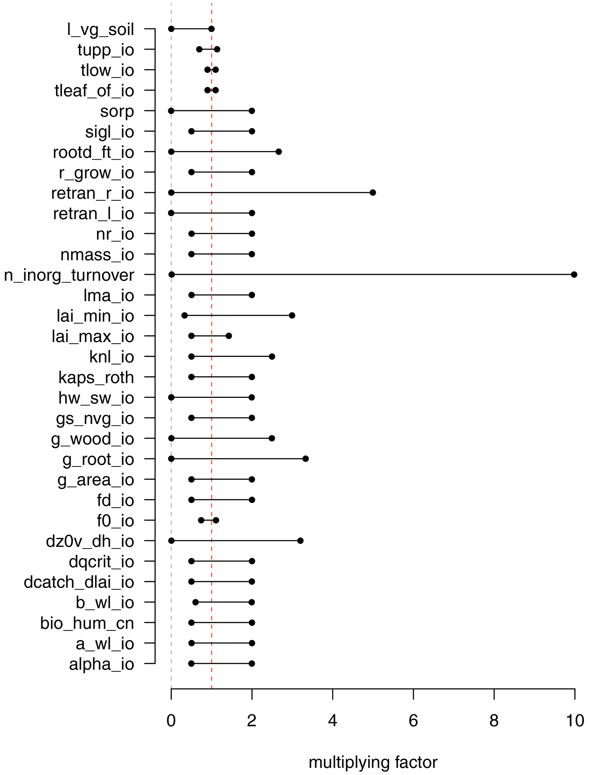
The initial ensemble must explore the limits of parameter space and ensure that any future constrained ensemble would be interpolating and not extrapolating from the initial design. We therefore asked model developers to set ranges on the parameter perturbations to be as wide as possible, while still having a good chance of running and at least providing output. We elicited reasonable multiplication factors from the modeller, based on the uncertainty for each parameter, and an estimate of the limits of the parameters at which the model would even run (see Fig. 1). The multiplication factors were perturbed in a space-filling design, in order to best cover input space and help build Gaussian process emulators, which can have problems if design points are spaced too closely. We chose a maximin Latin Hypercube design using the R package Latin Hypercube Samples or LHS (Carnell, 2021). The design chosen was the Latin hypercube with the largest minimum distance from a set of 10 000 generated candidates.

Many of the input parameters have different values for the 13 different PFTs in JULES. If each of these were perturbed independently, there would potentially be an intolerably large input space. Even accounting for the fact that many of the input settings would not be available (for example, perturbing some input values too far would effectively turn one PFT into another), the input space would still be of a very high dimension. In addition, each input setting would need careful thought from the modeller, and the resulting input space would be highly non-cuboid and complex. This would require a very large input of time and effort from both modellers and statisticians.

To combat this explosion of dimensions and effort, we chose the pragmatic option to perturb each of the PFTs together by a multiplication factor for each parameter. This choice was computationally convenient for a top-down, globally averaged experiment, but we see great potential for optimising the values of these parameters for individual PFTs in further work (a good example is Baker et al., 2022). Many of the multiplication factors varied the parameter range between half (0.5) and double (2) the parameter standard value. Some parameters were a switch and thus were set at zero or one. When the design was generated on a 0–1 axis, the design points were simply rounded to zero or one in this parameter.

Figure 1 Parameter multiplication factor ranges the initial ensemble (wave00) design.

2 Sequential constraint

Our iterated refocusing experiment uses a combination of formal and informal methods to sequentially constrain input parameter space and model behaviour, dependent on both expertise and expectation of the modellers, and on a more formal comparison with observational data. An important aim for the initial ensemble is primarily to train a good surrogate model, and therefore, we require relatively smooth output across the inputs space, without discontinuities or highly nonlinear behaviour that might bias an emulator. Our initial constraint procedures set out to achieve this.

Our initial (wave00) ensemble of 499 members is sequentially constrained to “level 0” by removing 24 ensemble members which do not run (see Sect. 2.1); to “level 1” by removing the 50 remaining ensemble member outside of the threshold in F0 (parameter 8) identified in Sect. 2.1; and to “level 1a” by removing the 64 remaining members outside the threshold in b_wl_io (parameter 4). This leaves us with a wave00 “level 1a” ensemble of 361 members that at least run and have a minimally functioning carbon cycle.

2.1 Failure analysis

We analyse the ensemble to remove ensemble members and corresponding parts of the parameter space that very obviously cannot hope to produce a useful simulation of the carbon cycle. First, we map ensemble members where the simulator failed to complete a simulation, perhaps due to numerical error (termed “failed”). Second, we identify parts of parameter space where important parts of the carbon cycle are completely missing – that is, basic carbon cycle quantities are at or close to zero at the end of the run (termed “zero-carbon cycle”). For this second class, we choose a threshold of mean modern global net primary production (NPP) close to zero ($<{\mathrm{10}}^{-\mathrm{5}}$). The nature of perturbed parameter ensembles is that there is often a setting of some parameters that makes up for a poor choice of a particular parameter, and so outright and easily identifiable thresholds for failure in the marginal range of a particular parameter are rare. However, careful visualisation and analysis can give the modeller a good idea of regions of parameter space that can be removed or parameters that the model is particularly sensitive to.

In Fig. 2, we see a pairs plot of failed runs (upper-right panels) and zero-carbon cycle panels (lower-left panels). The plot shows the two-dimensional projections of run failures against each pair of inputs, allowing visual identification of inputs that control failures, and any potential two-way interactions.

For example, we can see that both f0_io and b_wl_io have important thresholds, beyond which there appears almost no chance of a functioning carbon cycle. Inside these thresholds, if a run does not fail, it appears to always have a functioning carbon cycle of some sort. An interaction between the two presents as a nearly blank plot at the intersection of the parameters on the plot (row 8; column 4), with inputs identifying zero-carbon runs around the edges of the subplot. This indicates a region where nearly all non-failing ensemble members have a functioning carbon cycle. High values of b_wl_io result in the unphysical allometric scaling of vegetation height to biomass (e.g. 250 m tall trees).

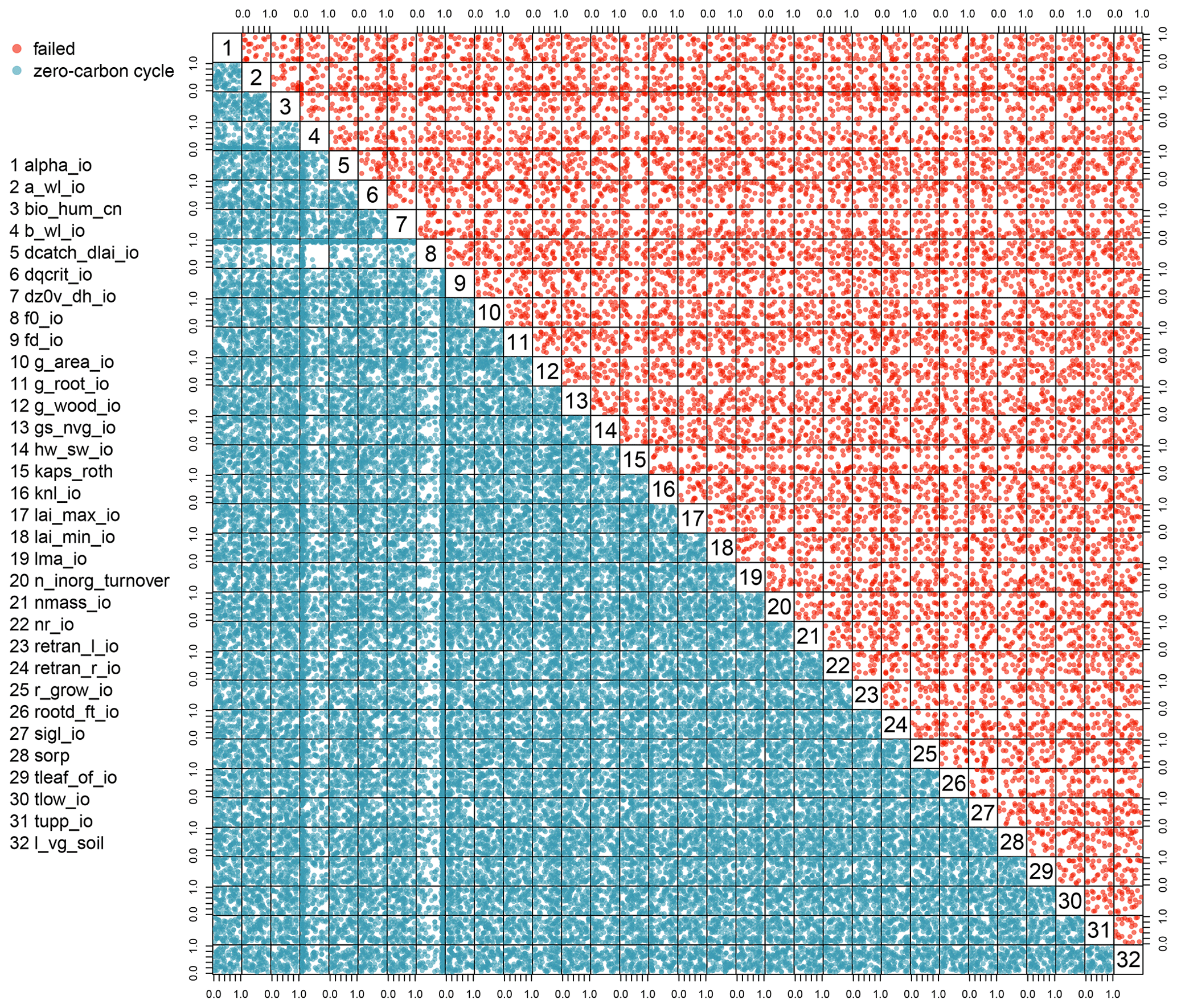
Figure 2 Two-dimensional projections of the input parameter values in a normalised input space of the ensemble members that failed or had a zero-carbon cycle.

2.2 First-wave results (level 1a constraint)

The globally averaged carbon cycle and land surface behaviour of the level 1a constrained ensemble can be seen in Fig. 3, and anomalies compared to the average of the first 20 years of the runs can be seen in Fig. 4 in the blue lines.

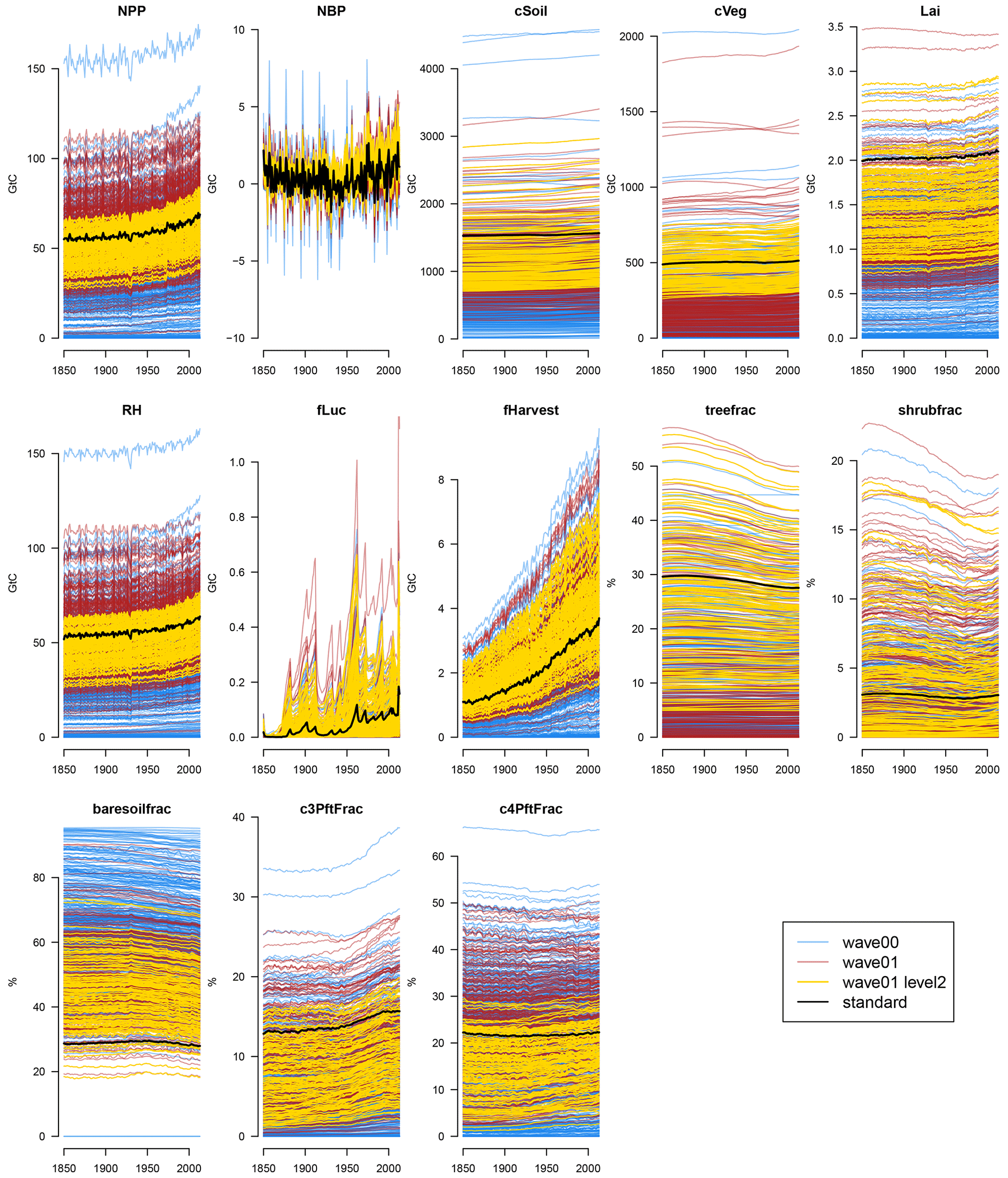
Figure 3 Time series of absolute carbon cycle quantities in the JULES ensemble at increasingly strict levels of constraint. The initial ensemble (wave00) is shown in blue, and the second ensemble (wave01) is shown in red. Ensemble members complying with the level 2 constraints are shown in yellow, and the ensemble member with standard parameter settings is shown in black.

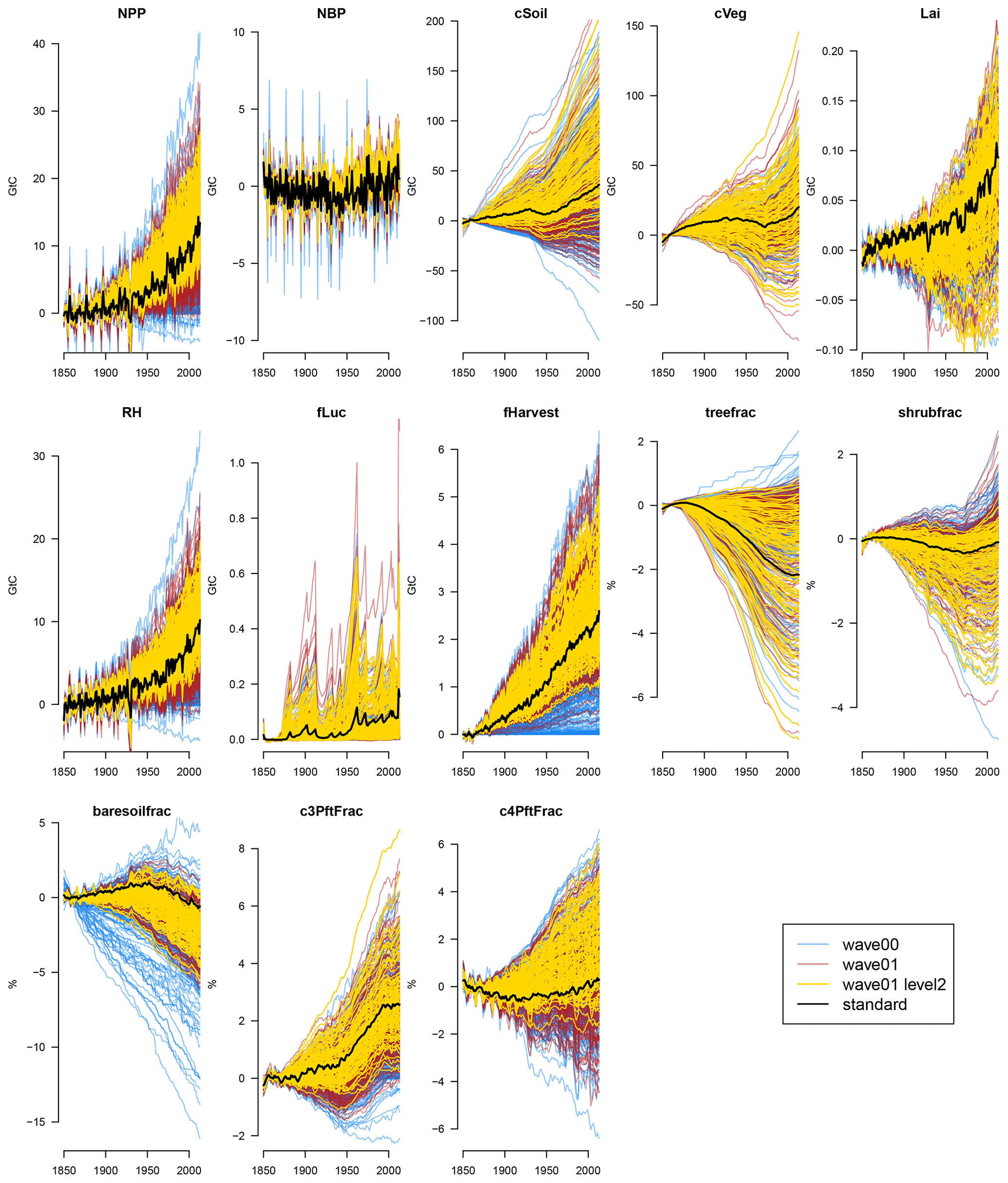
Figure 4 Time series of carbon cycle anomaly quantities in the JULES ensemble at increasingly strict levels of constraint. The initial ensemble (wave00) is shown in blue, and the second ensemble (wave01) is shown in red. Ensemble members complying with the level 2 constraints are shown in yellow, and the ensemble member with standard parameter settings is shown in black.

The ensemble displays a very wide range of both absolute levels and changes in a selection of carbon cycle and land surface properties, compared to the model run at standard settings (black). For example, global total NPP runs from approximately 0 to over 150 GtC yr⁻¹. Soil carbon stocks are between 0 and more than 4000 GtC, and vegetation stocks range from 0 to over 2000 GtC.

A large number of first-wave (wave00) ensemble members have a hugely diminished carbon cycle and carbon cycle stocks compared to the standard member. This can be seen from examining Fig. 3, compared to the values of the standard member (black lines). In particular, most ensemble members have a very low tree fraction and a higher bare soil fraction than the standard member. It seems particularly easy to kill global forests when perturbing parameters. Vegetation and soil carbon levels are also very low in many members.

Often, perturbing the parameters affects the overall level of the carbon cycle property, with its behaviour through time being only a secondary source of variance at the end of the model run. That is, the carbon cycle level at the end of the run is more closely related to its level at the beginning of the run than it is to its change over time. However, there is variability in the behaviour of the carbon cycle over time, as can be seen in Fig. 4. Here, we examine a selection of the most important carbon cycle properties and examine their change in behaviour over time or anomaly from the starting value. We see, for example, that changing the parameters can make soil and vegetation carbon increase or decrease over the simulated century and a half of the model run.

2.3 Level 2 constraints

We can constrain both the historical behaviour of the model and the model parameter input space by comparison of the model behaviour with the expectations of the model developers. Those expectations are set by the knowledge of independent observations of the real world or, when unavailable, by first principles and model simulations from independent groups.

A simple way to constrain the historical behaviour of the carbon cycle is by removing from the ensemble those model runs (and their corresponding input parameter settings) that lead to seemingly implausible values of basic carbon cycle quantities in the modern era. In this way, we are left with a subset of simulations and their corresponding input parameter sets that are consistent with our understanding of the true carbon cycle.

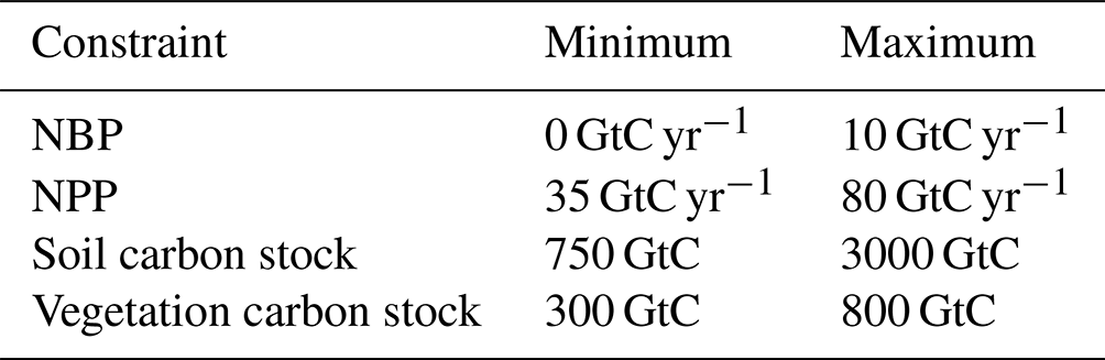
We choose a small number of broad constraints that the model must adhere to in order to be considered a valid and useful simulation. The constraints are four basic carbon cycle properties, globally averaged over the final 20 years of the simulations, near the beginning of the 21st century (1995–2014). They are net biome production (NBP; nbp_nlim_lnd_sum), net primary production (NPP; npp_nlim_lnd_sum), and the land surface stocks of soil and vegetation carbon (respectively, cSoil or cSoil_lnd_sum and cVeg or cVeg_lnd_sum). We choose generous limits on what might be called valid, roughly in line with the range of the CMIP5 Earth system model multi-model ensemble of opportunity. These constraints are outlined in Table 2. We designate these limits the level 2 constraints.

Only a very small proportion of ensemble members (38 out of 499) conform to the basic level 2 constraints expected of a useful model by our modeller. We would like to have a larger number of ensemble members in this range so that any emulator we build has enough detail to be useful and so that we can accurately map out viable input space. We wish to run more ensemble members within a valid input space, and so we formally history match to the level 2 space, in order to generate an input design for a second wave of ensemble members. We describe this process in Sect. 2.4.

Table 1 Increasing levels of constraint applied to simulator output during the experiment.

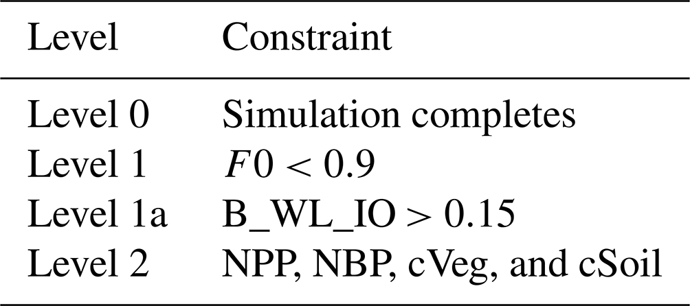
Table 2 Output limits to be met over the last 2 decades of simulation to match level 2 constraints.

2.4 History matching

History matching is a process whereby we formally compare the output of the model to observations of the real system and reject the parts of input parameter space where the model is not expected to plausibly simulate reality. Crucially, history matching recognises uncertainty both in the observations of the system and the model being used to simulate it. We use history matching to constrain the input space of the model, in order to both learn about inputs, and to find an input space which could credibly be used for future projections.

History matching has been used to great effect for constraining complex and computationally expensive simulators in a number of fields, including oil reservoir modelling (Craig et al., 1996, 1997), galaxy formation (Vernon et al., 2010, 2014), infectious diseases (Andrianakis et al., 2015), and climate modelling (Williamson et al., 2013, 2015; McNeall et al., 2020).

History matching measures the statistical distance between an observation of a real-world process and the predicted output of the climate model at an input parameter setting. An input where the model output is deemed too far from the corresponding observation is considered implausible and is ruled out. Remaining inputs are conditionally accepted as not ruled out yet (NROY), recognising that further information about the model or observations might yet rule them as implausible.

A vector representing the outputs of interest of the true land surface properties is denoted y. Observations of the system are denoted z, and we assume that they are made with uncorrelated and independent errors ϵ, such that

$$\begin{array}{}\text{(1)}& \mathit{z}=\mathit{y}+\mathit{ϵ}.\end{array}$$

The climate simulator is represented as an unknown deterministic function g(.) that runs at a vector of inputs x. As a statistical convenience, we imagine a best set of inputs x^*, which minimises the model discrepancy, δ, which represents the structural difference between the model and reality. In practice, this minimises the difference between climate model output g(x) and available observations z. We can therefore relate observations to inputs with

$$\begin{array}{}\text{(2)}& \mathit{z}=g\left({\mathit{x}}^{*}\right)+\mathit{\delta }+\mathit{ϵ}.\end{array}$$

The statistical distance between the simulator, run at a particular set of inputs x, and reality is measured using implausibility I:

$$\begin{array}{}\text{(3)}& I^{\mathrm{2}}=|\mathit{z}-E[g\left(\mathit{x}\right)]{|}^{\mathrm{2}}/(\mathrm{Var}\left[g\right(\mathit{x}\left)\right]+\mathrm{Var}\left[\mathit{\delta }\right]+\mathrm{Var}\left[\mathit{ϵ}\right]).\end{array}$$

This equation recognises that there is uncertainty in the output of the simulator and that this is estimated by an emulator. In this study, we use a Gaussian process emulator, described in Appendix C. Distance between the best estimate of the emulator and the observations must be normalised by uncertainty in the emulator Var[g(x)], in the observational error Var[ϵ], and in the estimate of model discrepancy Var[δ].

We reject any input as implausible where I>3, after Pukelsheim's three-sigma rule; that is, for any unimodal distribution, 95 % of the probability mass will be contained within 3 standard deviations of the mean (Pukelsheim, 1994).

2.5 Second-wave (wave01) design

We wish to generate design points for the second wave (wave01), which we believe will generate output that is not implausible; that is, where I<3 according to Eq. (3). As seen in the first wave (wave00), randomly sampling from across a priori plausible input space generates a large number of ensemble members which do not look like reality. Our strategy to increase the proportion which generates realistic output is to use the Gaussian process emulator to predict model output, generate a large number of potential candidates for new design points, and then history match to reject candidates we believe will lead to implausible output.

After building a Gaussian process emulator for each of the four modern value constraint outputs (NBP, NPP, cSoil, and cVeg), we generate a large number (50 000) of samples uniformly from the a priori not implausible input space. We calculate I for each of these samples and for each of the four outputs.

To calculate I, we set our observation as the midpoint of the tolerated range set by the modeller (see Table 2) and assume that the limits correspond to the 95 % range of an implied distribution (i.e. the range of the limits is assumed to cover 4 standard deviations of uncertainty in the assumed distribution). We assume that the expected model discrepancy is zero and that the uncertainty in the model discrepancy is also vanishingly small. In effect, this means that most of the uncertainty budget comes from the emulator and the observations.

From the subset of samples where I<3 (i.e. NROY) for all four outputs, we sample 500 potential design candidates and calculate the minimum distance between them in input space. We do this 500 times and choose the set with the largest minimum distance. This is to ensure that no two points are too close together, which can cause numerical errors when re-building the Gaussian process emulators. This set is then used to run the second-wave ensemble (wave01).

2.6 Second-wave results

A summary of the output of the second wave in the modern constraint variables can be seen in Fig. 5, compared to the same output from the first wave, constrained to level 1a. There is no simple relationship which allows us to calculate the number of ensemble members of the second wave that we expect to fall within the constraints. As history matching proceeds, input spaces can become very small, complex, and even discontinuous, resulting in difficulties in using standard Monte Carlo techniques to sample from them (Williamson and Vernon, 2013), even with guidance from the history matching process. The majority of the second-wave ensemble members fall outside of our level 2 constraints, but we see that the proportion of ensemble members in the second wave that match the constraints is much higher than in our initial ensemble. Of the 500 new members, we keep back 100 for validation purposes in future studies. Of the remaining 400, 128 (32 %) conform to all four constraints, compared with 27 out of 499 (7.4 %) of the initial ensemble. We find that the majority of ensemble members in the second wave fall within any one individual constraint. It is only when these constraints are combined that the majority are ruled out. A possible cause of the relatively small number of ensemble members that fall into all of the level 2 constraints is one or more poor emulators. We investigate this possibility in Appendix D2 and conclude that this is likely the emulator for cVeg consistently predicting slightly low, particularly for the higher (and more realistic) values of cVeg. The average value of NBP, NPP, cSoil, and cVeg has moved up in the second wave. There are no ensemble members that fail to run in the second wave, and there are not any that have a zero-carbon world; but there are 10 that have numerical problems and unusual values in their time series, and these are excluded from our analysis. We do not know if these failures are caused by numerical problems at those settings or occur stochastically, and this has an impact on the validity of the emulator across parameter space. An examination of the pairs plot of the input space of these suggests that certain parameter settings may cause these failures, but a sample of 10 is too small to make conclusive statements. A further study, with a significantly larger or differently targeted ensemble would be needed to settle this question.

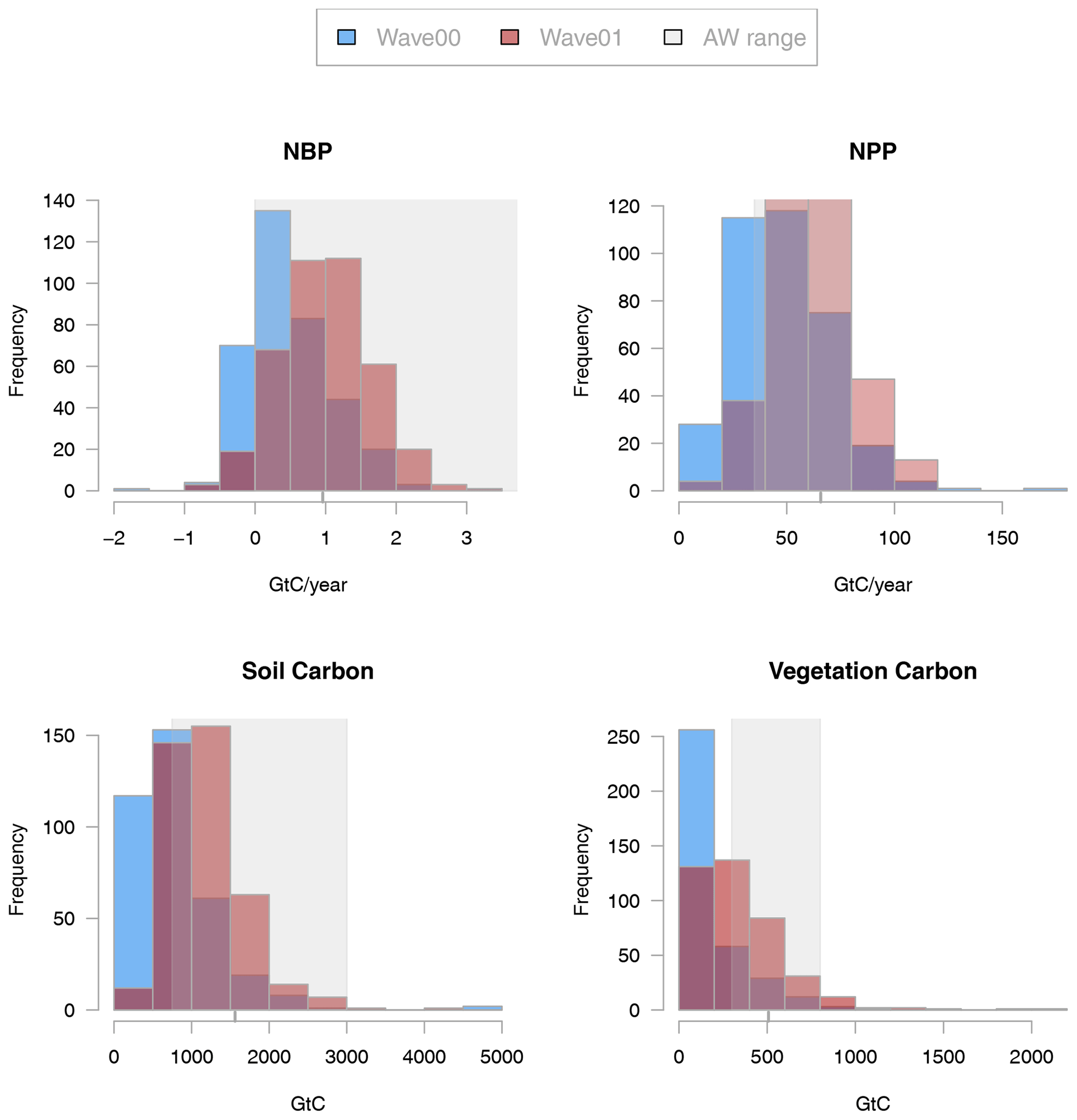
Figure 5 Histograms of ensemble output for the constraint outputs, namely global mean NBP, NPP, cVeg, and cSoil, in wave00 (blue) and wave01 (red). Shaded grey region indicates the constraints. Colours are semi-transparent, so darker purple indicates where the histograms overlap.

2.7 Induced constraints

In this section, we examine how imposing the level 2 constraints in NPP, NBP, cVeg, and cSoil automatically constrains both the input parameter space and the range of other outputs of the ensemble.

2.7.1 Constraints in model outputs

A summary of the induced constraints can be seen in Fig. 6, calculated as the proportion of the range of the initial ensemble covered by the level-2-constrained ensemble in the 20-year mean at the end of the time series. We see considerable induced constraints in output, particularly in soil respiration (26 %), bare-soil fraction anomaly (29.9 %), soil respiration anomaly (40.5 %), and C₄ plant fraction (43.9 %), which all reduce the ensemble range to less than 50 % of the original range.

While a useful measure, this is somewhat prone to outliers in the initial ensemble, and so examining the time series in Figs. 3 and 4 is recommended to give more context.

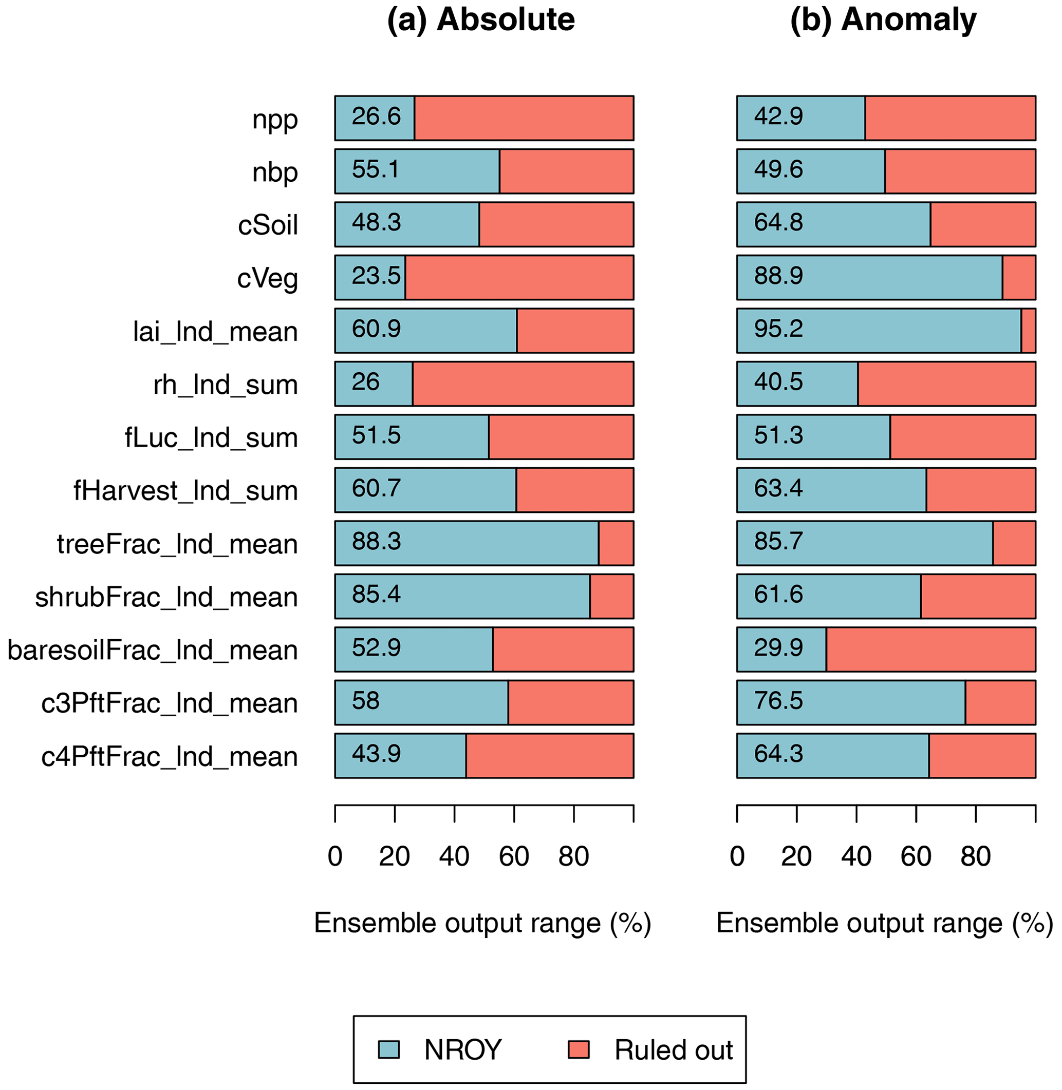
Figure 6 Proportion of the range of all output spanned by the level-2-constrained ensemble. The outputs are absolute values of the global mean values for 1995–2014 (a) and the anomaly of those values from the 1850–1870 values (b).

We see time series of the second-wave ensemble in Fig. 3 and anomaly time series in Fig. 4. The raw wave01 ensemble is coloured red, and the subset of ensemble members that conform to the level 2 constraints is coloured yellow. We can see a considerable constraint (as expected) in the time series of the constraint variables (NPP, NBP, cSoil, and cVeg). However, we also see constraints of varying magnitude across all other outputs.

Ignoring outliers, significant induced constraints are also visible in the leaf area index (LAI), crop harvest carbon flux (fHarvest), tree fraction (treefrac), and others. Our hypothesis is that our cVeg constraint enforces a minimum level of tree cover and therefore excludes high cover of other PFTs and bare soil. Such a constraint also seems to exclude low values of LAI. Our NPP constraint likely excludes low harvest flux and low values of soil respiration (RH).

Present-day constraints act to constrain historical anomalies in some of the variables, suggesting that uncertainty in some future projections might also be reduced. We see, for example, that constraining present-day levels of the carbon cycle variables induces a constraint (narrows the range of anomalies) in NPP trends, soil moisture trends, and carbon flux due to harvest but not overall NBP trends, which are made up of other elements. The anomalies in cSoil are constrained slightly, and the biggest historical losses of vegetation carbon (and corresponding increase in bare-soil fraction) are ruled out. Many (but not all) of the ensemble members that gain shrub fraction during the run are ruled out, particularly those that gain the most. Ensemble members with high C₄ grasses loss are ruled out. However, changes in vegetation carbon, leaf area index, and land use are constrained less.

In all cases, both for absolute values and anomaly values, the standard member lies well within the level-2-constrained ensemble, indicating that the standard member is consistent with observations. However, the standard member is often not central in the ensemble, suggesting that there may be sets of parameters which better represent the central tendency of our ensemble.

Further details are seen in Fig. 7, which plots two-dimensional projections of each pair of modern value model outputs against each other. The initial ensemble is shown in red, with the ensemble members passing the level 2 constraints (NROY) shown in blue. This plot gives valuable insight into how outputs vary together in the ensemble and how the constraints rule out large portions of output space, with the initial ensemble spread over a much wider output space than the constrained ensemble. For example, many corners of output space are ruled out, including for example simultaneously low values of soil respiration (rh_lnd_sum) and land use change carbon flux (fLuc_lnd_sum) or simultaneously low values of tree fraction (treeFrac_lnd_mean) and shrub fraction (shrubFrac_lnd_mean).

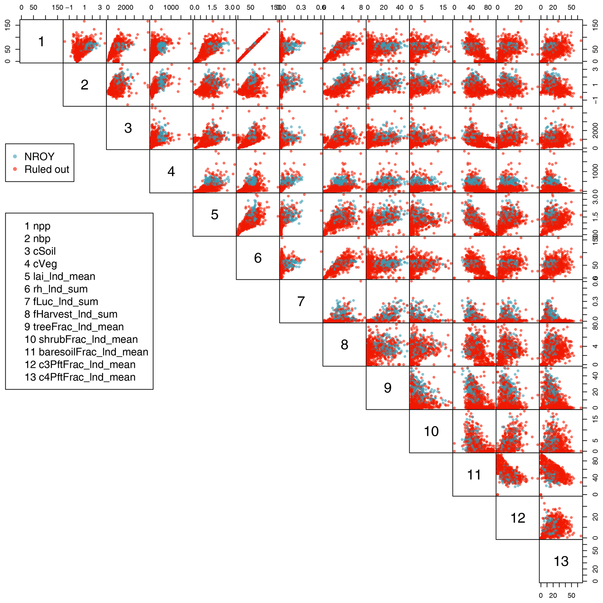
Figure 7 Two-dimensional projections of each pair of modern value model outputs. The initial ensemble is shown in red, with the ensemble members passing the level 2 constraints (not ruled out yet, NROY) shown in blue.

2.7.2 Constraining input space with an emulator

Rejecting implausible ensemble members based on their outputs gives a corresponding constraint on input space and sets limits for the parameter space where the model can be said to be behaving consistently with observations. Using the original ensemble members produces a useful but rough constraint outline of this valid input space. With only 38 ensemble members in the first wave, we were able to outline the valid 32 dimensional input space only very approximately.

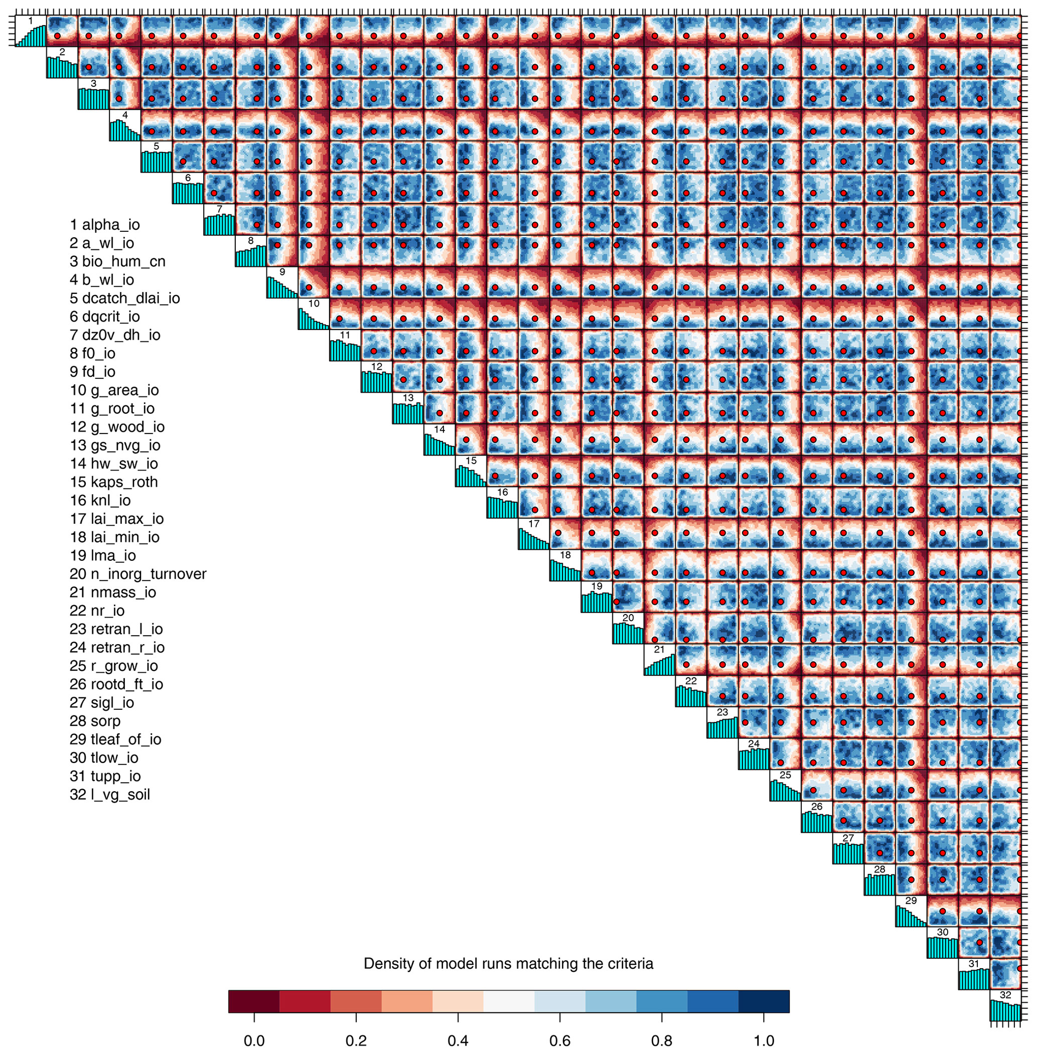
Figure 8 Two-dimensional projections of the density of input parameter candidates that conform to level 2 constraints. Blue regions have a higher density of points and red regions lower. Marginal histograms indicate the marginal density. Red points mark the standard input parameter value.

Using an emulator helps us visualise and quantify the constraint of input space when we constrain output space. After training an emulator on the relationship between model inputs and outputs, we can use that emulator in place of the full simulator JULES-ES-1.0, examining in more detail the inputs where the emulator predicts that the simulated outputs would match our constraints. Because the emulator is orders of magnitude cheaper to evaluate, we can take many thousands of samples from the input space and predict whether the simulator would match the constraints. This means that diagrams that summarise the input spaces can show densities of input points with a much higher resolution. The trade-off is that the emulator does not perfectly predict simulator output, and so visualisations of constrained input space are approximate. However, we judge that the emulator is accurate enough to provide useful insights, given the error and validation studies in Appendix D.

We fit a Gaussian process emulator to each of the modern constraint outputs, using the 751 members of both ensemble waves that have a non-zero-carbon cycle. We take 10⁵ samples uniformly from across the original normalised input space and reject all emulated members where the corresponding mean predicted output does not conform to the level 2 constraints.

We calculate the proportion of space that conforms to the level 2 constraints as approximately the proportion of samples that conform. A large number of samples ensures that the sampling uncertainty is small. Approximately 12 % of the initial input space conforms to all four level 2 constraints, meaning that our constraints have rejected approximately 88 % of initial input space as being incompatible with modern carbon cycle observations.

We plot two-dimensional projections of the density of accepted points in Fig. 8, colour coded by relative density. Blue areas show regions where there is a high concentration of accepted points, and we would expect a high probability of a model run at this input location producing a valid carbon cycle. Red areas in the diagram show regions of the input space where very few ensemble members are accepted as being consistent with observations. A red point marks the position of the standard set of parameters.

The diagram shows that some combinations of inputs have markedly smaller regions with a high relative chance of an input being accepted as consistent with observations. For example, only the region of simultaneously low f0_io and g_area_io has a relatively high chance of being accepted as being consistent with observations. Simultaneously high values of these parameters do not tend to give acceptable model output, and this corner of the input space can be ruled out.

Marginal histograms are plotted on the diagonal of the diagram, giving an indication of how many emulated ensemble members are accepted across their entire marginal range. For example, it is clear that low values of alpha_io are almost never accepted. It is possible to find some combination of the other parameters which compensates for low values of alpha_io, however, and so the absolute marginal range of alpha_io is not reduced. This does not mean that the input space is not constrained; it only means that we have constrained the joint space of parameters but not the marginal space.

It is worth noting that the default parameter (red dot) appears mainly in the blue regions of the diagram and produces output itself which is consistent with constraints. The fact that it is near the border of the acceptable input parameter space for some inputs gives the modeller an indication of which direction the default parameter could be moved in, while keeping the model output consistent with observations. For example, the parameter alpha_io could be safely increased, but decreasing its value would lower the chance of acceptable model output.

3 Sensitivity analysis

Global sensitivity analysis calculates the impact of changes in input parameters on simulator outputs, when inputs are perturbed across the entire valid input space. This is in contrast to a local sensitivity analysis, which calculates the impacts of small deviations from a set of default values. The two types of analysis are useful in different contexts. In our case, we have large uncertainties relating to a number of inputs, model processes, and observations, and so a global sensitivity analysis as a form of screening of important input parameters is appropriate.

We use a set of Gaussian process emulators, fit to each of the JULES-ES-1.0 land surface summary outputs, to perform two types of global sensitivity analysis. We use the set of Gaussian process emulators, fit to each of the outputs used for our level 2 constraint, for a third kind of sensitivity analysis. Each type of sensitivity analysis tells us different things about the relationship between the inputs and outputs of JULES-ES-1.0. At the end of this section, we summarise the results of all three types of sensitivity analysis in order to suggest which inputs might be prioritised in any future experiment.

Our aim is to give the modeller quantitative information on which inputs affect which outputs, to direct the effort for reducing model biases and errors, and to indicate regions of parameter space where the model might perform better. We might identify parameters which have a direct impact on the model output that does not conform to observations, identify groups of parameters within a poorly performing process, or help modellers sample uncertainty in other model applications.

3.1 Global one-at-a-time sensitivity

A one-at-a-time (OAAT) sensitivity gives a simple and easy-to-interpret measure of the impact of each input on a variety of outputs but does not include the effects of any interactions between inputs (for example, a non-linear change in model outputs as two or more inputs vary together).

An OAAT analysis can be completed with a relatively small number of model runs; for example, a low, middle, and high run for each parameter in our 32-input-dimension example would take fewer than 100 runs. However, using an emulator allows us to better characterise the response of the model across the entire range of each parameter, which would take many more dedicated runs if completed using just the model.

We fit a Gaussian process emulator to each global summary output, both as a modern value (mean of 1995–2014) and as an anomaly (change since 1850–1869). We use the 751 members from both wave00 and wave01 that conform to the level 1a constraints, making as wide an input space as possible without significant model failure.

We sample from the input space in a one-at-a-time fashion; each input is sampled uniformly across its input space, with all other inputs held at standard values (note that these are often not the central value when normalised to the 0–1 range). The variance of the mean emulated output as each input is varied is then used as a measure of the sensitivity of that output to the corresponding input. Variance is used as opposed to magnitude of change, as we expect some model outputs not to rise or fall monotonically as an input varies.

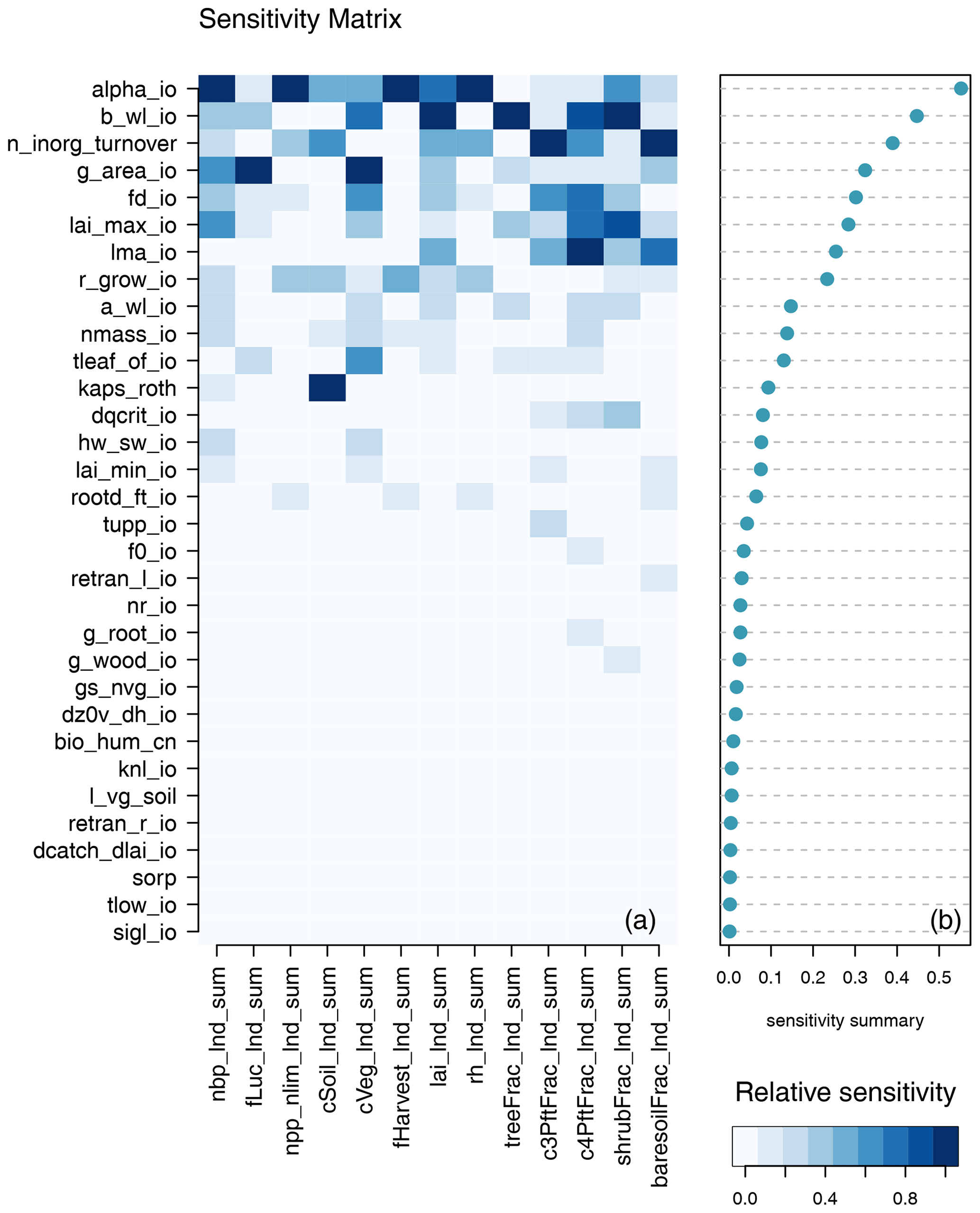
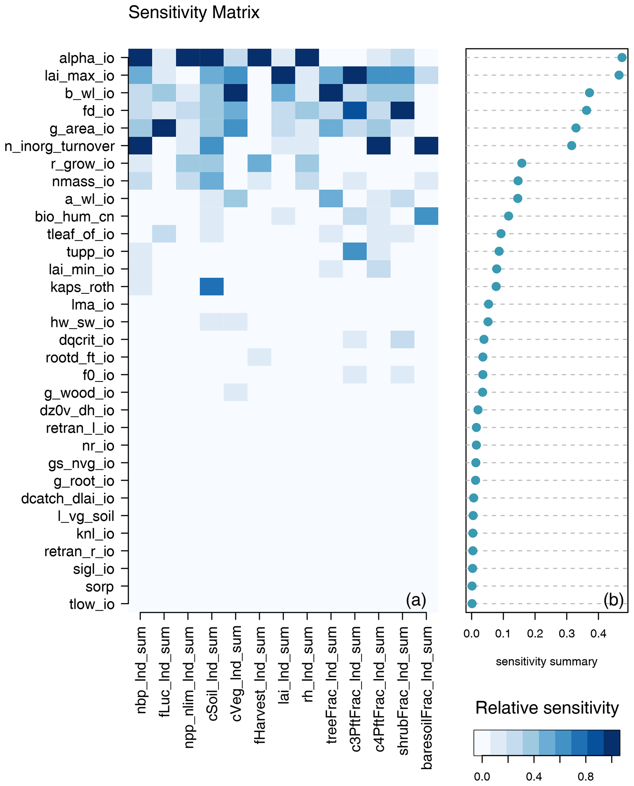
Different model outputs are clearly sensitive to different model inputs, and so we also seek ways of summarising sensitivity across model outputs. One method is simply to find the mean effect across model outputs. Sensitivities are normalised so that they lie in a [0−1] range for each output. Summary measures for each input are then averaged across all outputs, and the plotted inputs are ranked by their average influence across all outputs. Individual sensitivities and summaries can be seen in Fig. 9 for the modern value and in Fig. 10 for the change over the historic period of the ensemble. The right-hand side of each diagram shows the average of the sensitivity measures by which the input parameters are ranked in their influence. We see that for both the modern value and anomaly only half or fewer of the inputs have discernible impact on global outputs by this measure.

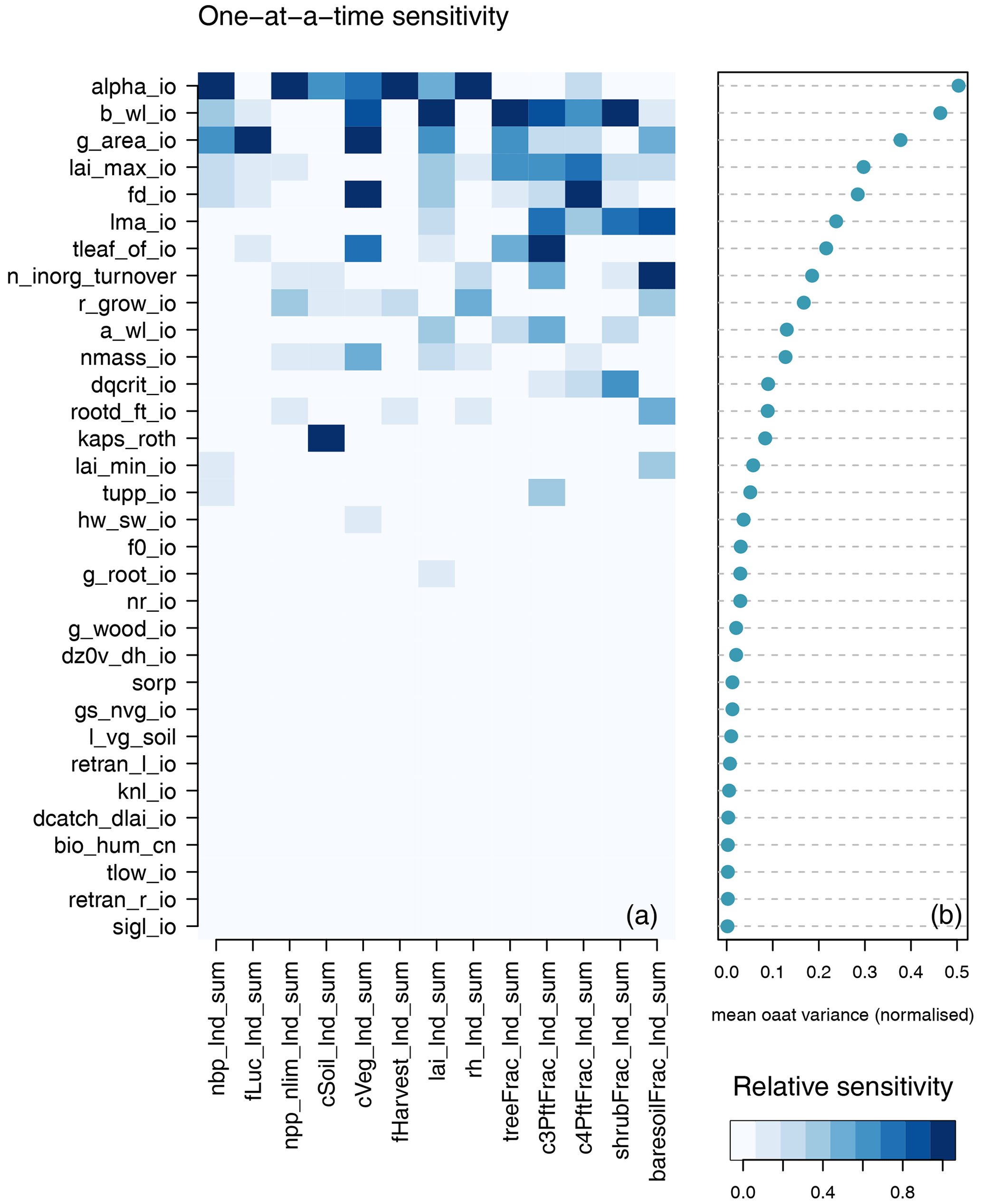
Figure 9 One-at-a-time sensitivity summary for global summary modern value output. Panel (a) shows the relationship between each individual input and output. Panel (b) shows the average of the sensitivity measures by which the inputs are ranked.

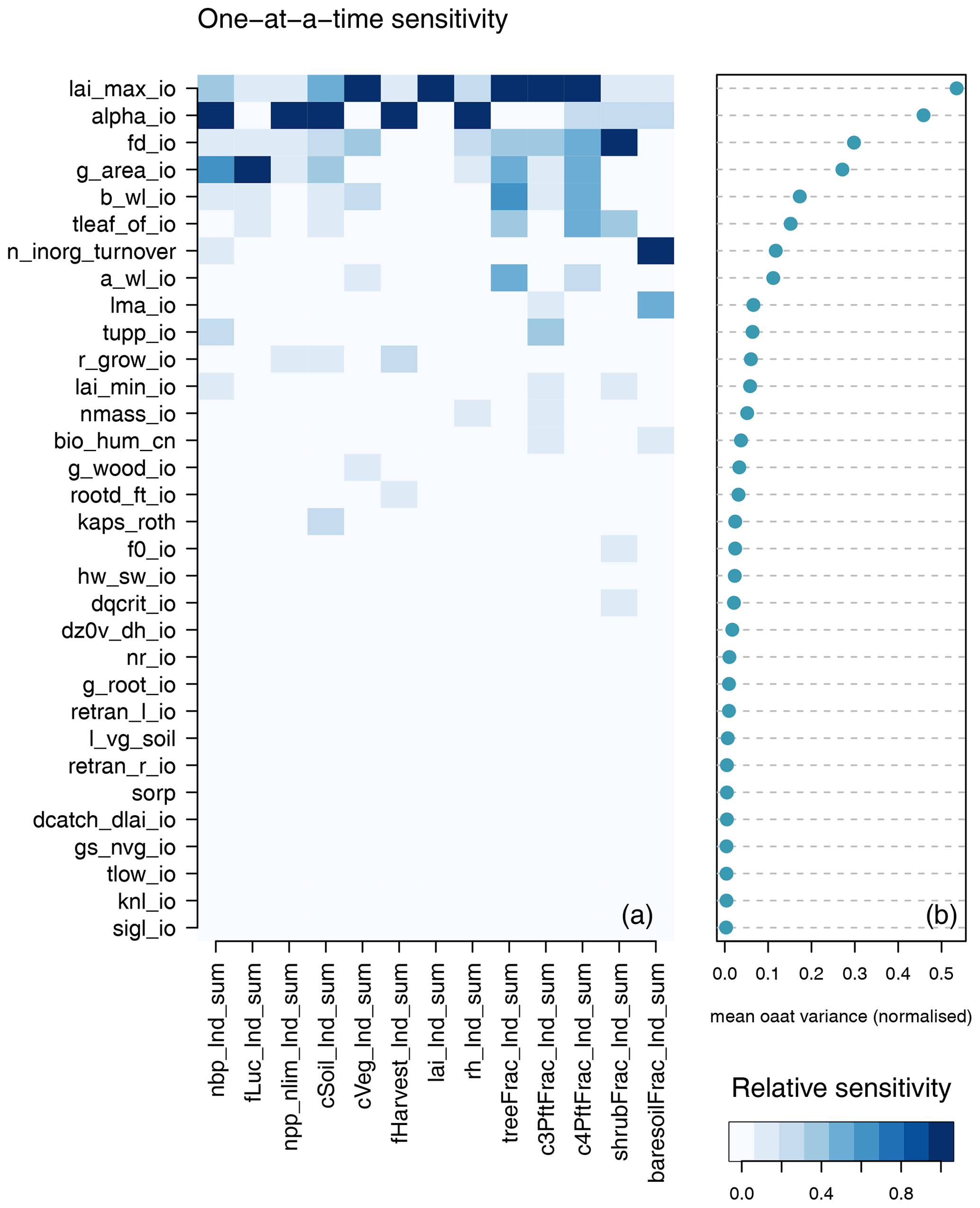
Figure 10 One-at-a-time sensitivity summary for global summary anomaly (change since 1850–1870) output. Panel (a) shows the relationship between each individual input and output. Panel(b) shows the average of the sensitivity measures by which the inputs are ranked.

3.2 Sensitivity of constraint outputs

We add detail to our one-at-at-time sensitivity of important outputs, namely those that we use for constraining JULES-ES-1.0 in Fig. 11. We plot the emulated mean of the each of four outputs – NBP, NPP, vegetation carbon, and soil carbon – as each parameter is increased from its minimum to maximum range. Uncertainty bounds from the emulator predictions are not plotted, in order to more clearly see the estimated main effect of each parameter, but uncertainty estimates for the emulators can be seen in Appendix D1.1. For each input, we can see the default value as a vertical dashed line. This plot indicates how deficiencies in the model output might be corrected by altering individual parameters. For example, the fact that many ensemble members have low-vegetation carbon might be countered by increasing alpha_io or nmass_io or reducing g_area_io or tleaf_io. Of course, these alterations will not be without impact on other model outputs, causing changes which might be countered elsewhere or must be weighted against improvements in a particular output.

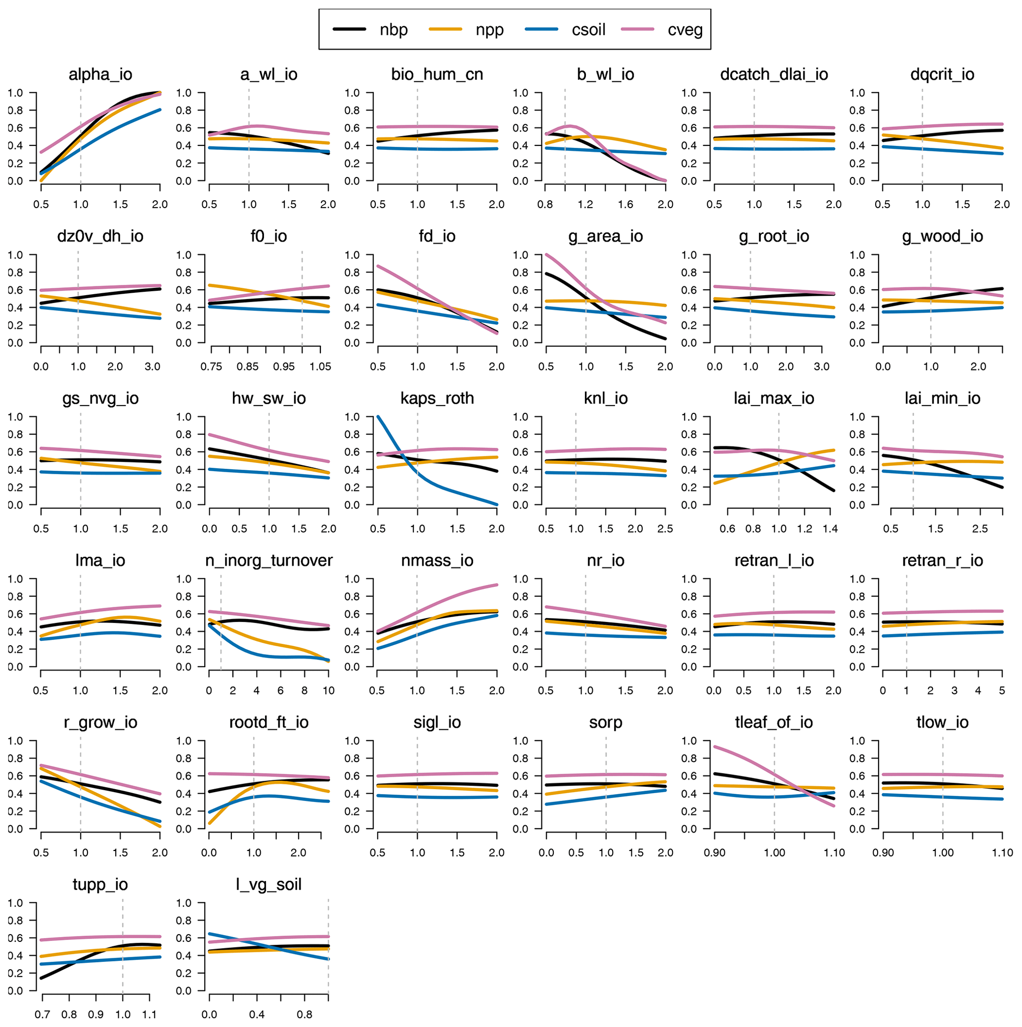
Figure 11 One-at-a-time sensitivity summary for global summary of the modern value of the constraint variables (NBP, NPP, cVeg, and cSoil).

3.3 FAST sensitivity analysis

We use Fourier Amplitude Sensitivity Test (FAST) as a further measure of global sensitivity of the model outputs to its inputs. The test is administered as the FAST99 algorithm of Saltelli et al. (1999), through the R package Sensitivity (Pujol et al., 2015). Again, this algorithm requires a large number of model runs, and so we use emulated model outputs in place of dedicated model runs (as previously used in McNeall et al., 2020, 2016; Carslaw et al., 2013). This comes at the cost of a risk of inaccuracy, as the emulated model outputs will not perfectly reproduce the true model runs at the corresponding inputs. However, the emulator is shown to work adequately for the model outputs in Appendix D.

A FAST gives both first-order and interaction effects; we sum these together to calculate a total sensitivity index and to make showing the results across a large number of outputs simpler. Individual results for FAST can be seen in Appendix F, and the summarised results are used in our analysis in Sect. 3.5

3.4 Monte Carlo filtering

Monte Carlo filtering (MCF) is a type of sensitivity analysis that integrates well with our aim of constraining model behaviour, given a large ensemble using ensemble member rejection or history matching. The idea of MCF is to identify inputs that have an influence on whether the behaviour of the model falls within or outside acceptable bounds. This is done by splitting samples of model behaviour into those that do or do not meet some constraint and then summarising the difference between the cumulative distributions of the corresponding input variables. The larger the difference between the cumulative distributions, the more influence the parameter has on whether the model passes the constraint.

A description of MCF and its uses can be found in Pianosi et al. (2016). McNeall et al. (2020) use MCF to estimate parameter sensitivity in the land surface model element of a climate model of intermediate complexity.

We use a Gaussian process emulator to allow a much larger set of samples from the input space, in order to make the MCF process more efficient, at the cost of inaccuracy if the emulator is poor. We train a Gaussian process emulator on each of the four constraint outputs, using the 751 ensemble members from both wave00 and wave01 that pass the level 1a constraints. We draw a large sample of 10 000 parameter combinations, which are uniformly from the level 1a input parameter distributions. We use the emulator to estimate the true model output for each of the four constraining variables, namely NPP, NBP, cVeg, and cSoil, at these parameter values. We perform a two-sample Kolmogorov–Smirnov (KS) test on the cumulative distributions of those input samples, where the mean of the emulator predicts that the model would be within or outside of the modeller's level 2 constraints. We use this KS statistic as an indicator of the sensitivity of the model output to each input. We summarise the sensitivity in Fig. 12.

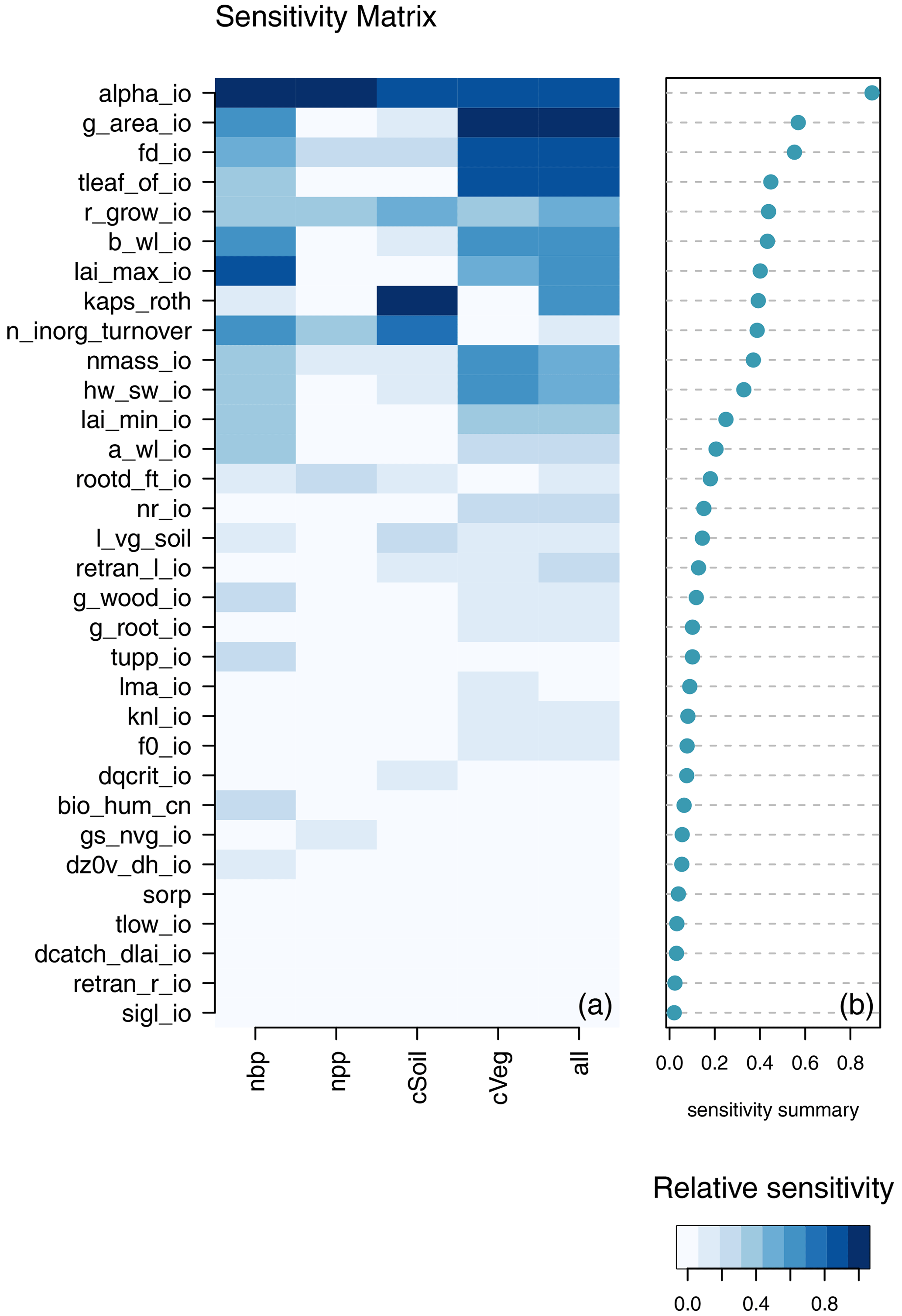
Figure 12 Monte Carlo filter sensitivity summary for a global summary of the modern value of the constraint variables (NBP, NPP, cVeg, and cSoil). Panel (a) shows the relationship between each individual input and output. Panel (b) shows the average of the sensitivity measures by which the inputs are ranked.

3.5 Screening input variables by ranking

Which parameters would we include in a subset of parameters for a new ensemble? One way to choose might be to exclude those parameters which are inactive; i.e. those that have a small or no effect on any model output of interest under any of our tested measures of sensitivity. For this ensemble, we screen out these inactive inputs by ranking the inputs using each of the sensitivity measures. We can test OAAT and FAST SA for both modern value and anomaly for the entire set of inputs. We can test the MCF for the set of constraint outputs that we measure against real-world observations (or modellers' expectations).

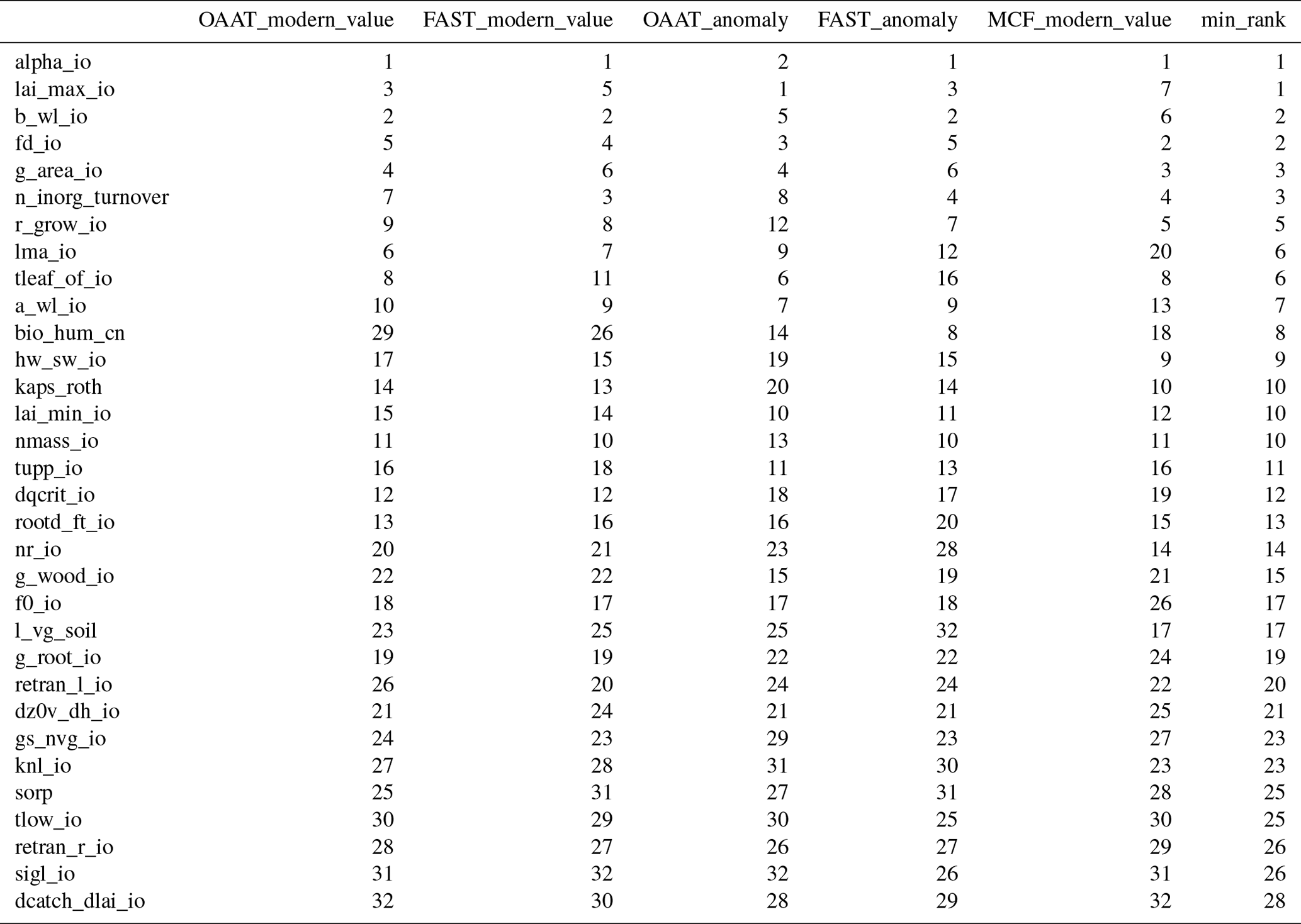
A conservative strategy excludes only those inputs that are consistently ranked lowest; that is, those that have the lowest minimum ranking (or those with highest value of the rank). While we might choose a number of strategies for weighting outputs to prioritise input sensitivity, a good start might be to focus on the constraint outputs and later moving towards other output comparisons. We see, for example, in Table 3 that 17 of the parameters never appear in the top 10 most important inputs for any measure. Depending on our criteria for any new design, we would preferentially disregard inputs that never achieved a high rank.

Using different measures of sensitivity makes our decisions more robust. However, a potential problem with the approach is that all of the sensitivity analyses share a Gaussian process emulator and so will be sensitive to any errors or biases in that shared emulator. It is crucial that model developers are satisfied with the performance of the emulator across the relevant parts of input parameter space and its associated outputs.

Table 3 Summary sensitivity ranks for all carbon cycle outputs, modern value, and anomaly, for three different types of sensitivity analysis.

4 Discussion

In this section, we discuss the results of the constraint process and the sensitivity analysis and what they tell us about the model.

4.1 Lessons learnt

As an exploratory and no-regrets analysis, a key outcome of this experiment is to identify the lessons learnt from it, if we would do things differently if we did the experiment again, and what we might take from it to future experiments.

First, would we use the top-down or data-led approach, where we perturb all inputs simultaneously, across wide parameter ranges, and constrain with global mean output again? If we did, could it be improved? This approach provides a rapid and efficient first look at how model parameters influence global output. It is useful for an initial screening of the parameters and to see which inputs broadly do or do not affect our outputs of interest. It reduces the chances that there may be some unidentified parts of input space where the model would perform better; perhaps we have some discrepancy that can easily be resolved through tuning? The top-down approach might help us set parameter boundaries in situations where strong prior knowledge about what the parameters should be is not there.

However, the approach has its limitations and inefficiencies. First, as we see in Sect. 2.2, many runs fail to complete or have highly unrealistic output (e.g. zero-carbon cycle) in the initial ensemble. Only a very small number (less than 10 %) came within the generously wide observational constraints on output. This was perhaps inevitable, given the approach of halving and doubling the most unknown inputs. Furthermore, the halving and doubling approach leaves the standard member far from the centre of the ensemble, which can perhaps lead to an overemphasis on parts of the input parameter space that were, in hindsight, unlikely to produce good output.

A more careful initial expert elicitation of input parameters might help to target more realistic uncertainty bounds for these parameters, although at a cost of more human time spent on the elicitation process and a higher chance of missing good (but a priori unlikely) parts of parameter space. While these kind of experiments can effectively trade the computation and analysis time for set-up time, the optimal balance of these is often unclear until after the experiment.

With so many free parameters, there are often ways to offset any model discrepancy that can be attributed to a certain parameter by adjusting another parameter. In this case, it becomes hard to rule out the marginal limits of a parameter when there is always another parameter whose impact can offset it. This means that it is difficult to advise modellers on hard constraints for their input parameters. Many constraints will be joint; that is, they will depend on the plausible setting of other parameters. We often see, with this kind of set-up, a constraint that has ruled out the large majority (88 %) of input space as inconsistent with the observations yet has not completely ruled out any marginal input space for individual parameters.

How could this problem be addressed? One way of shrinking down marginal space might be to add more data comparisons, thus increasing the chance that a parameter will be deemed implausible in a history matching exercise, for example. A problem with adding more data until much of the input space is ruled out, however, is that the chance of an unidentified but significant model discrepancy goes up, particularly if some parts of the climate model are deemed more important and may have had more development attention than others. In this scenario, a significant model error could lead to analysts unjustifiably ruling out parameter space that should be retained.

A counteraction to this problem might be found in a sequential approach. Perhaps this can be done by targeting particular outputs (and inputs) that are deemed more important in order to get right, before proceeding to data observation comparisons where relationships are more uncertain. The later data observation comparisons would carry less weight, and a modelling judgement could be made as to the cut-off point where the analysis continued to add value. Our sensitivity analysis might also help here; narrowing down the most important inputs to perturb in a repeat (or continuation) of the experiment could significantly simplify the input parameter space under investigation.

Another strategy might be a simple vote system of constraints, whereby an input is excluded if a number of model outputs fail to meet expectations at a particular input, or a more involved history matching process. A number of multivariate approaches to history matching have been taken in the past, usually either using a maximum value of implausibility or using a mean squared error approach to calculate an overall implausibility of an input (see, e.g., Vernon et al., 2010).

5 Conclusions and further work

In this study, we were able to produce a perturbed parameter ensemble of land surface simulations and associated parameter sets using JULES-ES-1.0, consistent with our understanding and observations of the true behaviour of the land surface and considerably more tightly constrained than an initial ensemble.

An initial design, purposely chosen to produce a wide range of ensemble behaviour, generated only a very small number of members ($\mathrm{37}/\mathrm{499}$) that would conform to a set of four basic constraints on global carbon cycle and land surface properties. In this first wave (wave00) of model simulations, there were identifiable marginal limits for parameters b_wl_io and f0_io that caused the simulation to fail or to produce zero-carbon-cycle climates. These limits were quite near the initial design limits and removing outliers therefore did not shrink input space much.

We were able to train Gaussian process emulators of global mean summaries of many land surface properties, with mean absolute errors all less than 10 % of the span of the ensemble. After using the emulators to predict outputs that would fall within reasonable constraints in the four key outputs, a much higher proportion (128 of 400 members) of a second wave of simulations complied with the constraints. Emulator performance improved for most outputs after adding data from the second wave to the training set, particularly for those members that passed the level 2 constraints. This means that analyses will be more accurate and have less uncertainty than they would have when training with only the initial ensemble. When constraining input space to level 2, using the four basic observational constraints and the emulator removed 88 % of initial input parameter space, but marginal ranges were hard to constrain. There were induced constraints of varying degrees when the ensemble output was constrained by using the four carbon cycle observations.

We used three types of global sensitivity analysis to identify the most (and least) important parameters. A number of inputs which have very little impact on global output were identified and would be recommended to be excluded from further analyses in order to simplify the input space and improve emulator performance. Detailed information on the relationship between individual parameters and global mean outputs will be useful to modellers identifying ways to improve the simulator. A focus on the key uncertain parameters will be useful for modellers and to inform future improvements of JULES ahead of the next generation Earth system models.

The potential of observations to further constrain input parameter space could and should be explored. Both more waves of simulations – further improving emulators and reducing uncertainty – and new observations of unconstrained outputs could be tried. Care must be taken to ensure that adding more observations does not unduly increase the chances of including an unidentified simulator discrepancy.

We might identify parts of the parameter space where the model does better at reproducing observations, rather than simply removing parts of the parameter space where the model does poorly. Regions that produce more realistic carbon vegetation (cVeg), for example, or airborne fraction could be targeted in an optimisation or calibration routine. A simple analysis could illustrate parts of the input parameter space that do better than the standard ensemble member.

Finally, we could use sensitivity analysis and uncertainty quantification to quantify the impact that observations of the land surface might have on the uncertainty of future projections and the parameters by which that uncertainty is manifest. A useful extension to this study would identify which observations would best constrain future projections of the carbon cycle and by how much.

In summary, we have successfully constrained the input space and corresponding output space for simulating the carbon cycle with the JULES-ES model. As part of the process, we gained lots of valuable insight into the threshold behaviour associated with certain parameters and the marginal impact of parameter settings. This information is extremely useful in arriving at a single parameter set for the full complexity Earth system model for which only a single parameter set is realisable. Ultimately, the analyses used here could be extended, and applied to future experiments, to better understand and constrain terrestrial carbon cycle feedbacks – a key uncertainty in setting carbon budgets necessary to meet the Paris Agreement climate goals.

Appendix A: Parameters

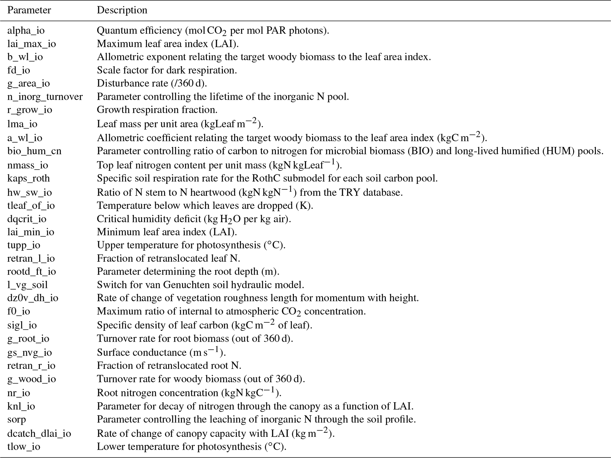
A set of input parameters and their descriptions can be seen in Table A1.

Table A1 Uncertain input parameters in JULES-ES-1p0.

Appendix B: Outputs

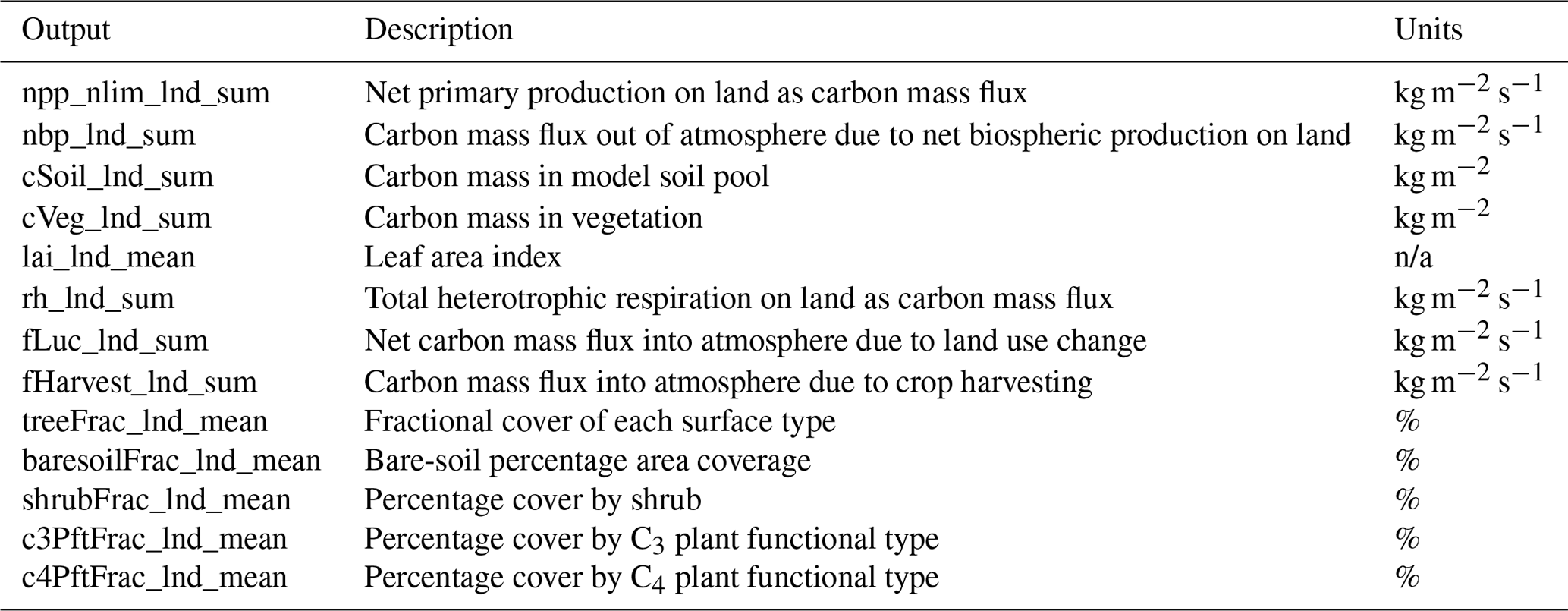
A set of land surface and carbon cycle outputs of JULES-ES-1.0 and their descriptions can be seen in Table B1.

Table B1 Uncertain input parameters in JULES-ES-1p0. n/a – not applicable

Appendix C: The emulator

As a summary univariate output of the simulator, land surface model JULES-ES-1.0, the term y is treated as an uncertain function f() of the input vector x so that y=f(x).

We produce a predictive distribution for y at any simulator input vector, conditional on the points already run or the design (Y,X). We use a kriging function, or a Gaussian process (GP) regression emulator, from the package DiceKriging (Roustant et al., 2012) in the statistical programming environment R (R Core Team, 2016).

The GP regression is specified hierarchically with a separate mean and covariance function. For prediction purposes, we assume that the trend is a linear function of the inputs x and adjust with a GP.

$$f\left(\mathit{x}\right)=h(\mathit{x}{)}^T\mathit{\beta }+Z(\mathit{x}),$$

where h(x)^Tβ is a mean function, and the residual process Z is a zero-mean stationary GP. The covariance kernel c of Z

$$\mathrm{Cov}(\mathbf{Z},{\mathbf{Z}}^{\prime })={\mathit{\sigma }}^{\mathrm{2}}c(\mathit{x},{\mathit{x}}^{\prime })$$

can be specified in a number of different ways: we use the default option of a Matern $v=\mathrm{5}/\mathrm{2}$ function so that

$$\begin{array}{rl}c(\mathit{x},{\mathit{x}}^{\prime })& =\left(\mathrm{1}+{\displaystyle \frac{\sqrt{\mathrm{5}}|\mathit{x}-{\mathit{x}}^{\prime }|}{\mathit{\theta }}}+{\displaystyle \frac{\mathrm{5}|\mathit{x}-{\mathit{x}}^{\prime }{|}^{\mathrm{2}}}{\mathrm{3}{\mathit{\theta }}^{\mathrm{2}}}}\right)\\ & \exp \left(-{\displaystyle \frac{\sqrt{\mathrm{5}}|\mathit{x}-{\mathit{x}}^{\prime }|}{\mathit{\theta }}}\right),\end{array}$$

where θ describes the characteristic length scales (or roughness parameters), which are a measure of how quickly information about the function is lost moving away from a design point in any dimension.

These, along with other hyperparameters, are estimated via maximum likelihood estimation from the training set (Y,X), so the approach is not fully Bayesian. We use universal kriging with no nugget term, meaning that there is zero uncertainty for model outputs in the training set, and the mean prediction is forced through those points.

Details of the universal kriging process used can be found in Sect. 2.1, the kernel in Sect. 2.3, and examples of trend and hyperparameter estimation in Sect. 3 of Roustant et al. (2012).

Appendix D: How good is the emulator?

We assess the quality of the Gaussian process emulator for a number of outputs that we use for constraining the parameters of JULES.

Although there are a large number of possible metrics for validating emulators (see, e.g., Al-Taweel, 2018), we prefer those that give the modeller information about the performance of the emulator in terms of the output of the model and the context of the entire ensemble. As such, we wish to relate the performance directly to the model output and to metrics that make sense and are important to the modeller. Although the uncertainty estimate of a particular the emulator prediction is important, it takes a secondary role to the performance of the posterior mean prediction in our work.

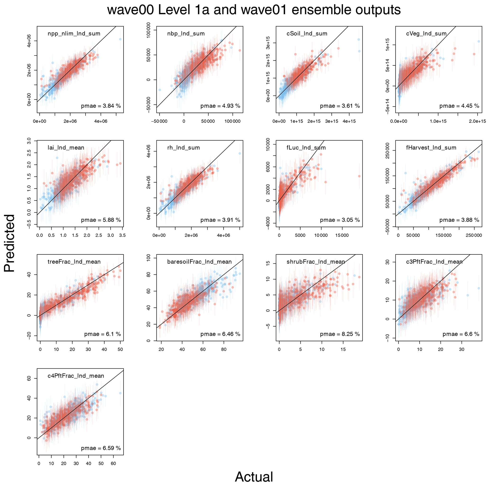
Figure D1 Leave-one-out summaries of emulator fits for modern value carbon cycle quantities. The first wave (wave00) is blue, and the second wave (wave01) is red.

D1 Leave-one-out metrics

We use a leave-one-out prediction metric to initially assess the quality of our Gaussian process emulators. For each of the outputs of interest, each of the 361 ensemble members which form the level-1a-constrained ensemble is removed in turn. A Gaussian process emulator is trained in its absence and then the withheld ensemble member is predicted. We repeat the process while adding the 390 successful members of the second wave (wave01), in order to assess the value of adding extra training points for the emulator.

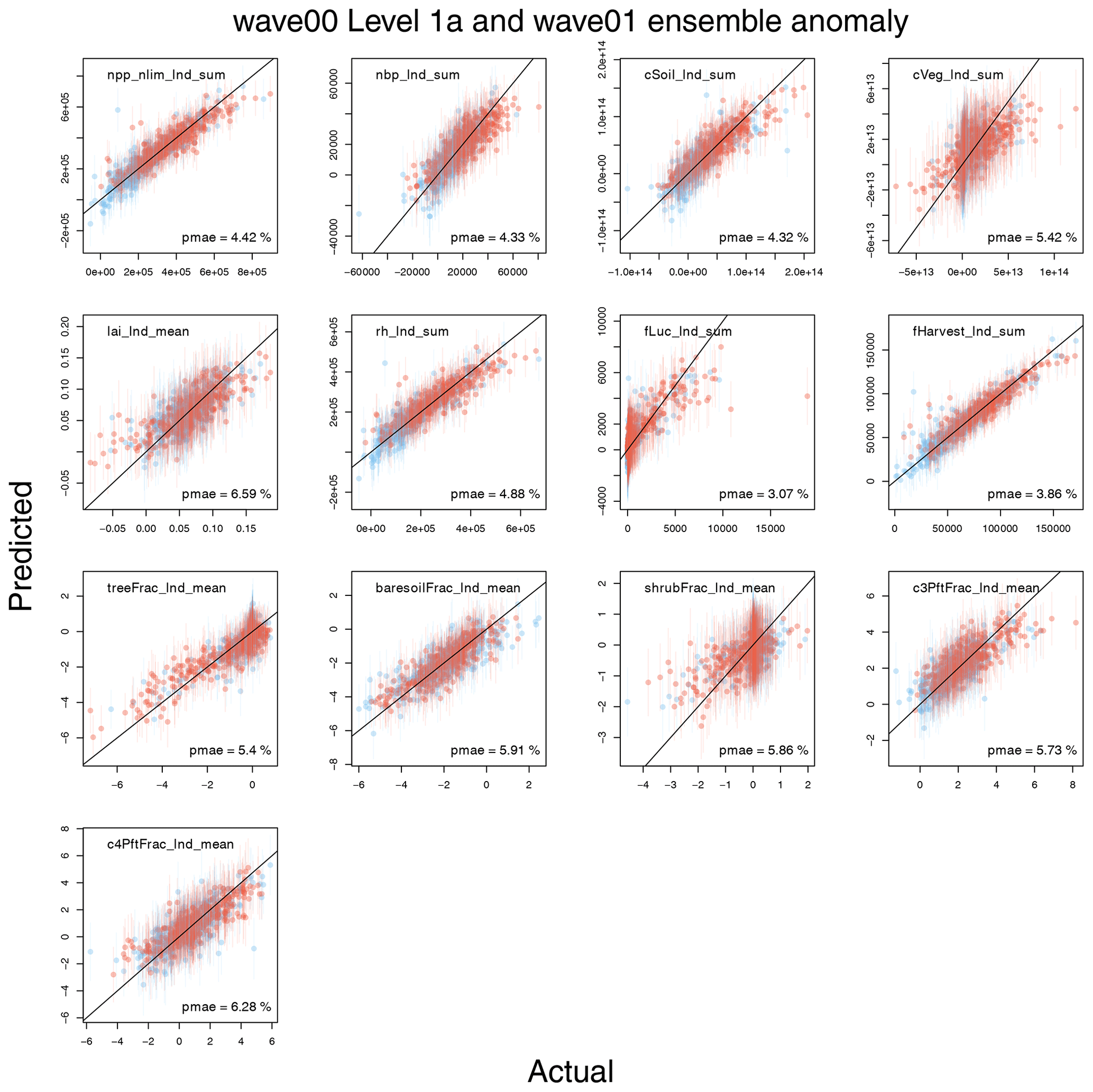
Figure D2 Leave-one-out summaries of emulator fits for modern value anomaly carbon cycle quantities. The first wave (wave00) is blue, and the second wave (wave01) is red.

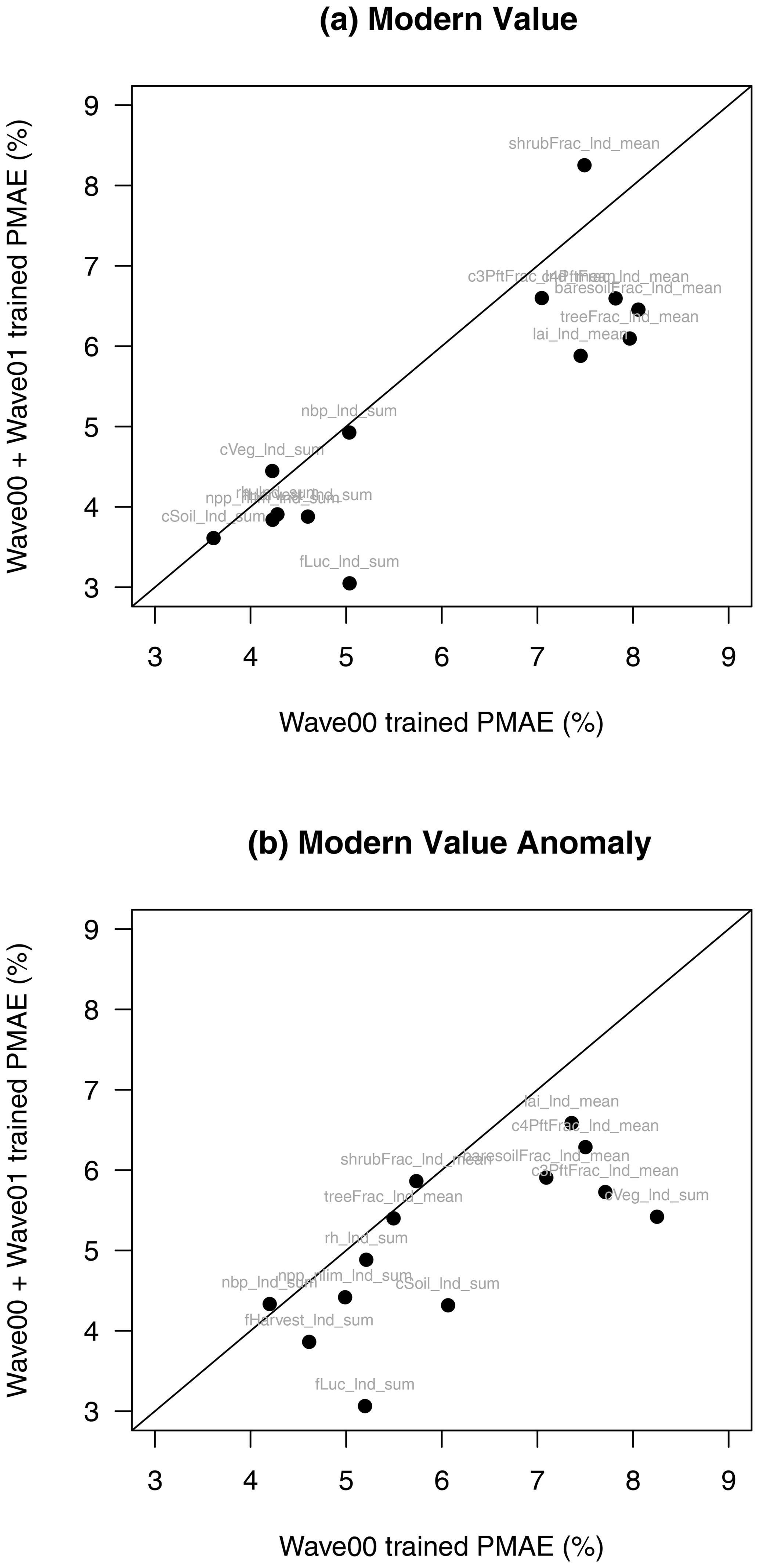
Figure D3 Proportional mean absolute error (PMAE) summaries for selected JULES modern value (a) and anomaly (b) outputs. Horizontal axes show PMAE using only wave00 level-1a-constrained outputs, while vertical axes show the same summary using wave00 and wave01 outputs. Outputs below the diagonal line show an overall improvement in emulator performance.

Figures D1 and D2 show summary plots of the actual value against the predicted value (the mean of the Gaussian process), and associated uncertainty (±2 standard deviations) for each output, for both modern values and anomaly, or for change in the output over the duration of the simulation. For each output, we include a summary of the performance across the ensemble in the form of the proportional mean absolute error (PMAE), which we define as the mean absolute error in the prediction when that error is expressed as a fraction of the range of the ensemble. The PMAE is calculated when all 751 members are used to train each GP emulator.

For the modern value, we find that the PMAE ranges from between around 3 % and around 8 % of the range of the ensemble, with the emulator for fLuc_lnd_sum performing best (PMAE = 3.05 %) and shrubfrac_lnd_sum performing worst (PMAE = 8.25 %).

For the anomaly output, we find a similar range, with the emulator for fLuc_lnd_sum anomaly scoring a PMAE of 3.07 % and the poorest performance of c4PftFrac_lnd_mean anomaly scoring a PMAE of 6.59 % (Fig. D2).

We see the value of including the extra ensemble members in the training set in Fig. D3. For both the modern value and anomaly outputs, we plot PMAE using the emulators trained with the 361 wave00 level 1a ensemble with those trained, including the former plus the 390 wave01 ensemble. Points below the diagonal line show an improvement in the performance of the emulator for that output. Not all emulators show an increase in performance using this metric, but the vast majority do.

D1.1 Assessing emulator variance

To assess emulator variance, we produced rank histograms (Hamill, 2001) for the emulators of the 13 modern value outputs, both for absolute (Fig. D4) and for anomaly (Fig. D5) outputs. Leave-one-out tests were conducted for the 751 ensemble members of wave00 (level 1a) and wave01 combined. For each ensemble member, 1000 predictions were simulated from the prediction distribution and ranked, and the rank of the observation was compared. A well-calibrated prediction produces a uniform distribution of the ranks across ensemble members. A domed shape in the histogram indicates that uncertainty is overestimated (i.e. we do better in the prediction than we think), and a U shape indicates that uncertainty is underestimated.

We see that most emulators have well-calibrated uncertainty estimates, without obvious deviations from uniform histograms. Exceptions are perhaps apparent in outputs fLuc_lnd_sum, fHarvest_lnd_sum, and cVeg_lnd_sum, which show a distribution weighted near the centre of the histogram. In all of these cases, this indicates a mild overestimate of uncertainty, which is less concerning than an underestimate of uncertainty. In this case, we can be more confident of the behaviour of the mean of the emulator prediction than our uncertainty estimate would indicate.

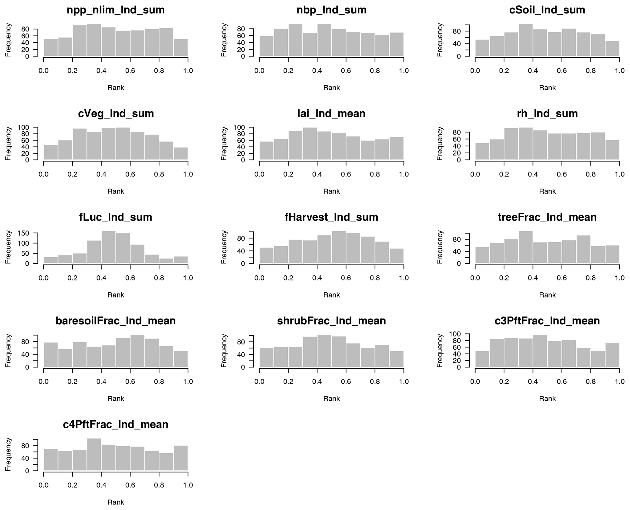
Figure D4 Rank histogram to test the emulator uncertainty estimate for 13 modern value 1 outputs, covering the absolute values of major land surface and carbon cycle outputs of JULES-ES-1.0. A uniform distribution indicates a well-calibrated uncertainty estimate. A domed shape indicates overestimated uncertainties, while a U shape indicates underestimated uncertainties.

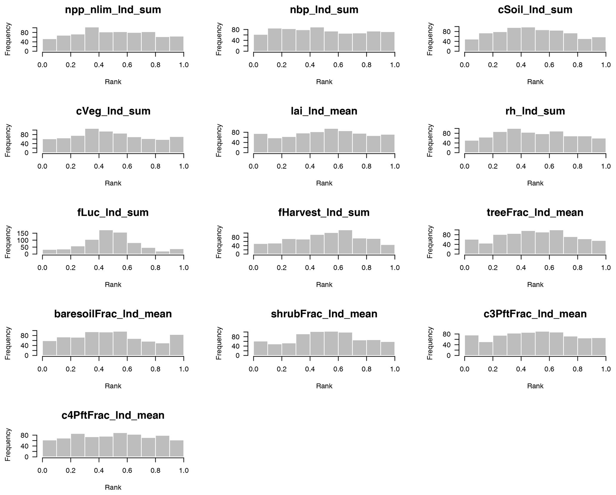
Figure D5 Rank histogram to test the emulator uncertainty estimate for 13 modern value outputs, covering the anomaly values of major land surface and carbon cycle outputs of JULES-ES-1.0. A uniform distribution indicates a well-calibrated uncertainty estimate. A domed shape indicates overestimated uncertainties, while a U shape indicates underestimated uncertainties.

D2 Predicting members that satisfy level 2 constraints

A useful measure of the practical utility of our emulator is the accuracy with which we can predict if a given input configuration will produce model output that conforms to a set of constraints. Here, we focus on the accuracy of our emulator for predicting ensemble members that conform to our reasonable level 2 constraints. These ensemble members produce output that is reasonable in a very broad way; i.e. roughly consistent with a functioning carbon cycle, our observations of the world, and the CMIP6 ensemble but not directed at a particular set of observations.

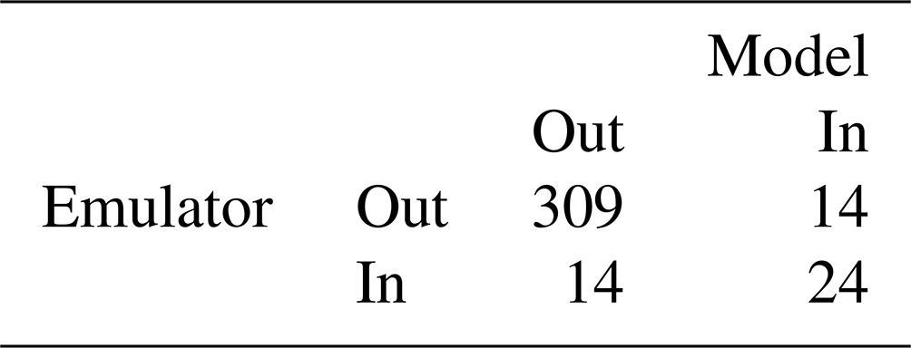
We perform a leave-one-out cross-validation on the outputs that we use for the level 2 constraint, namely the modern-day value of the global sum of NBP, NPP, soil carbon, and vegetation carbon. We show the results of the leave-one-out posterior mean predictions in Fig. D6. If we treat the posterior mean predictions as model runs and constrain them using the same thresholds as the level 2 results, then we can convert them into a binary forecast for whether they are in or out of the constraint. While this loses some information, it is a useful summary. We predict 24 ensemble members correctly as being in the constraints and 309 correctly as being out. We predict 14 incorrectly as being out when they should be in (false negative) and 14 incorrectly as being in when they should be out. A contingency table summarising these results is presented in Table D1. We use the R verification package (NCAR – Research Applications Laboratory, 2015) to calculate a number of skill scores, including the equitable threat score (ETS), which we calculate at 0.34, and the Heidke skill score (HSS), which we calculate at 0.51. These scores (as well as the raw numbers) indicate that we have a predictive system, which could well be improved.

Table D1 Confusion matrix for leave-one-out emulator predictions of whether the true model outputs conform to the level 2 output constraints. Correct predictions are on the diagonal of the table.

Studying Fig. D6, we see that a possible culprit for many of the constraint prediction errors is the relatively poor quality of the emulator for vegetation carbon (cVeg). That emulator predicts a relatively large number of ensemble members to have a lower vegetation carbon compared to we see in reality (and many close to zero) when the true vegetation is high. This leads to a number of false negatives. Conversely, when the vegetation carbon is relatively low, there are a small number being over-predicted, leading to false positives. This is not a consistent bias, so we cannot simply add a discrepancy value all across the input space; more subtlety is required in order to improve the emulator and predictions.

We try a number of strategies to improve the emulator, including transformation of the cVeg output by taking logs or using the square root. These can considerably improve the emulator for low values of the output. Unfortunately, we do not believe that the very low values are realistic and are therefore not very informative about higher values. Indeed, transforming the output has the impact of making the leave-one-out scores for the ensemble members that conform to level 2 constraints worse. We try a number of different covariance types and optimisation methods within the emulator fitting process for cVeg, but none improves the performance for level-2-conforming ensemble members.

It appears that the initial design for the experiment was set too wide, with many ensemble members having unrealistically low carbon vegetation values. This meant that this emulator is difficult to build, output is not smooth, and the constraint may well benefit from an iteration of the history matching, getting the initial ranges more close to being correct, and having a smoother output.

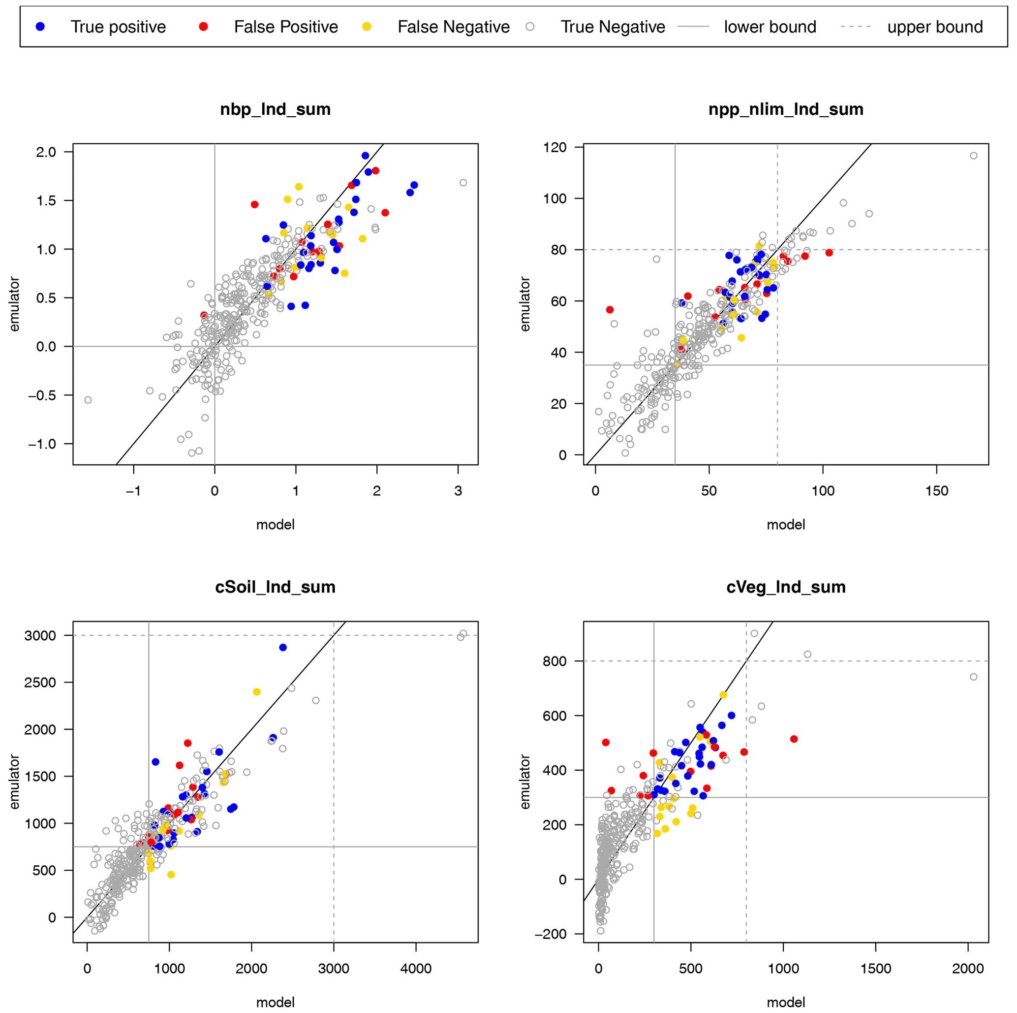
Figure D6 Leave-one-out predictions of the status of the initial ensemble members that are either in or out of the level 2 constraints in NBP, NPP, cVeg, and cSoil.

Appendix E: Impact of uncertainty on the sensitivity analysis

We use visualisation to assess the impact of emulator uncertainty on the one-at-a-time sensitivity analysis in Fig. E1 (for modern value) and Fig. E2 (for modern value anomaly outputs of JULES-ES-1.0). Each row in the matrix of plots is an output, and each column is an input, so each individual plot shows an emulated estimate of how an output varies across an input when each input is varied independently. The emulator mean prediction is shown as a black line, and the emulator uncertainty is shown as a grey shaded area. Each row is normalised to the largest range of variability, so the reader can see the impact of each input in for each particular output. This plot allows the reader to see the magnitude of the variability relative to the emulator uncertainty. For some outputs (for example, treefrac_lnd_sum), the variability is much larger than the uncertainty. For some (for example, cVeg_lnd_sum), the uncertainty is relatively larger. However, it is possible in all outputs to identify the input parameters with the largest impact on outputs.

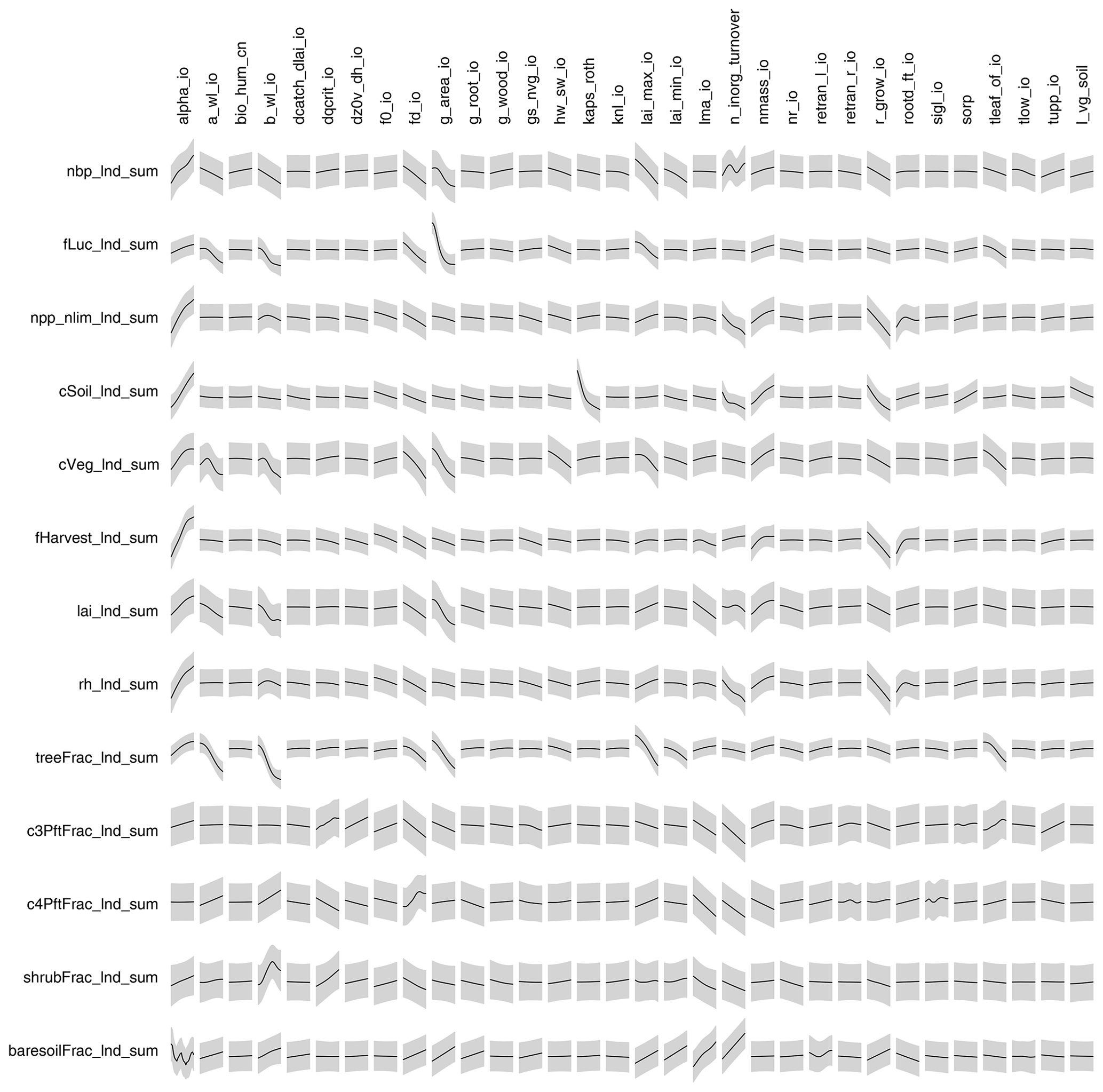
Figure E1 Impact of emulator uncertainty on the sensitivity analysis for modern value outputs.

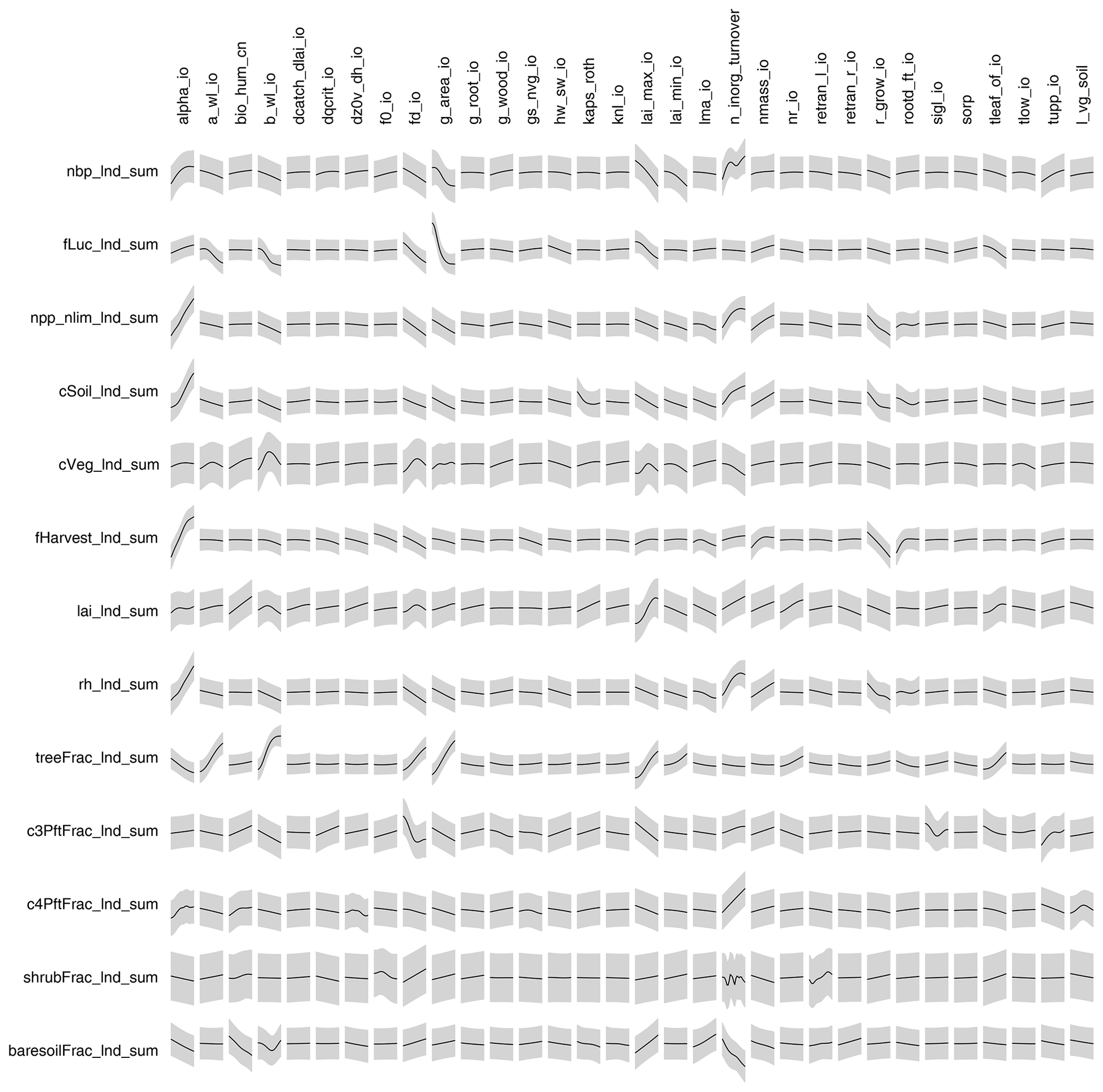
Figure E2 Impact of emulator uncertainty on the sensitivity analysis for modern value anomaly outputs.

Appendix F: FAST sensitivity analysis details

Summaries of FAST sensitivity analysis for both modern value and anomaly outputs of JULES-ES-1.0 can be found in Figs. F1 and F2, respectively.

Figure F1 FAST sensitivity analysis summary for modern value outputs.

Figure F2 FAST sensitivity analysis summary for anomaly outputs.