A gridded air quality forecast through fusing site-available machine learning predictions from RFSML v1.0 and chemical transport model results from GEOS-Chem v13.1.0 using the ensemble Kalman filter

Statistical methods, particularly machine learning models, have gained significant popularity in air quality predictions. These prediction models are commonly trained using the historical measurement datasets independently collected at the environmental monitoring stations and their operational forecasts in advance using inputs of the real-time ambient pollutant observations. Therefore, these high-quality machine learning models only provide site-available predictions and cannot solely be used as the operational forecast. In contrast, deterministic chemical transport models (CTMs), which simulate the full life cycles of air pollutants, provide predictions that are continuous in the 3D field. Despite their benefits, CTM predictions are typically biased, particularly on a fine scale, owing to the complex error sources due to the emission, transport, and removal of pollutants. In this study, we proposed a fusion of site-available machine learning prediction, which is from our regional feature selection-based machine learning model (RFSML v1.0), and a CTM prediction. Compared to the normal pure machine learning model, the fusion system provides a gridded prediction with relatively high accuracy. The prediction fusion was conducted using the Bayesian-theory-based ensemble Kalman filter (EnKF). Background error covariance was an essential part in the assimilation process. Ensemble CTM predictions driven by the perturbed emission inventories were initially used for representing their spatial covariance statistics, which could resolve the main part of the CTM error. In addition, a covariance inflation algorithm was designed to amplify the ensemble perturbations to account for other model errors next to the uncertainty in emission inputs. Model evaluation tests were conducted based on independent measurements. Our EnKF-based prediction fusion presented superior performance compared to the pure CTM. Moreover, covariance inflation further enhanced the fused prediction, particularly in cases of severe underestimation.

1 Introduction

Rapid economic growth and urbanization have led to severe ambient air pollution in China (Li et al., 2016a). Thanks to the National Air Pollution Prevention and Control Action Plan released in 2013 (The State Council of China, 2013), air quality has steadily improved. However, for the past decade, air pollution has still been ranked as the third major factor causing death in China, following tobacco and high blood pressure (GBD 2019 Risk Factors Collaborators, 2020). Approximately 80 % of the Chinese population is still exposed to fine particulate matter (PM_2.5), with annual mean concentrations exceeding 35 µg m⁻³, and over 99 % of the population is exposed to severe air pollution according to the World Health Organization air quality guideline value of 10 µg m⁻³. (Wang et al., 2019; Cheng et al., 2021b). Forecasting primary atmospheric pollutants with high spatial resolution is thus essential in order to provide early warning for residents and reduce detrimental public exposure to air pollution (Bi et al., 2022).

Machine learning methods, particularly deep learning tools, have gained significant popularity in geoscientific fields owing to their high accuracy and relatively low computational resource requirements. For instance, Chen et al. (2023) fully estimate hourly near-surface ozone concentration in China using a new geostationary satellite with the help of machine learning. Numerous studies have successfully implemented machine learning algorithms for air quality prediction. For example, Li et al. (2018) proposed a hybrid model combining a weighted extreme learning machine and an adaptive neuro-fuzzy inference system for air quality predictions. Ma et al. (2020) improved the accuracy of WRF-Chem prediction of daily PM_2.5 concentrations in Shanghai by applying an XGBoost machine learning method. Cheng et al. (2021c) successfully predicted ground-level daily maximum 8 h ozone concentrations in two megacities in China, Shanghai and Chengdu, by utilizing wavelet decomposition and two machine learning models. Mao et al. (2022) developed a dynamic graph convolutional approach and sequence to sequence embedded with the attention mechanism model for predicting daily maximum 8 h average ozone concentrations. We have successfully used the regional feature selection-based machine learning model (RFSML) to predict air quality with high accuracy. Our forecast system can provide short-term predictions for over 1262 sites across China at a national scale. We developed the SAGE (Shapley additive global importance) ensemble feature selection algorithm to exclude redundant inputs, which efficiently improves our forecasting ability (Fang et al., 2022). We trained these models using historical measurement datasets collected at independent air quality monitoring stations, and they operate using real-time air quality observations as inputs. However, unlike gridded forecasts, our predictions are only available for the location of the air quality monitoring sites. Meanwhile, the spatial distribution of existing environmental monitoring stations is rather uneven in China, with a dense monitoring network in the east and a sparse network in the west, as shown in Fig. 1. Therefore, our RFSML predictions limited to these few monitoring stations cannot accurately represent the true PM_2.5 concentrations on a national scale.

Deterministic 3D chemical transport models (CTMs) are widely used for operational air quality forecasting due to their ability to predict air pollution in continuous spatiotemporal domains by modeling complex physical and chemical processes of air pollutant life cycles. CTMs provide an advantage over machine-learning-based air quality forecast models, which typically rely on point-source observations. Various CTMs have been developed and employed for air quality forecasting. For example, Keller et al. (2021) provided a new modeling system, GEOS-CF, that can make 5 d forecasts of the concentrations of five primary ambient pollutants; Cheng et al. (2021a) developed a real-time forecasting system of hourly PM_2.5 concentrations using the WRF-CMAQ model in Taiwan. Lin et al. (2020) developed the WRF-GC model (coupling the Weather Research and Forecasting meteorological (WRF) and the GEOS-Chem model) that can perform high-resolution air pollutant forecasts. Using the WRF-Chem model, Georgiou et al. (2022) developed a high-resolution real-time air quality forecast system over the eastern Mediterranean with better performance than the Copernicus Atmosphere Monitoring Service. While these air quality forecast models can capture the spatiotemporal variations in ambient pollutants to some extent, they are susceptible to systematic bias, particularly at a fine scale, due to multi-source uncertainties in emission inventories (Keenan et al., 2009; Fan et al., 2018), initial and boundary conditions, and parameterization of physical and chemical processes such as transport and removal (Croft et al., 2012; Solazzo et al., 2017). This makes the CTM prediction less reliable for localized air quality predictions (Bi et al., 2022).

Both the machine learning models and CTMs have weakness when they are solely used in operational air quality forecasting. The same challenges exist when observations and simulation models are used to describe the atmospheric dynamics in reanalysis products. Observations are widely preferred due to their higher accuracy compared to numerical dispersion models. However, they are inherently limited in providing a continuous 3D field and cannot fully scan the entire target domain. On the other hand, models provide gridded simulation results but are typically biased as explained previously. To address the limitations of relying solely on observations or simulation models, Bayesian-theory-based assimilation methods (Evensen et al., 2022), by combining the observations and model simulations, have long been performed for producing gridded reanalysis that is much closer to reality. For example, the fifth generation of atmospheric reanalysis (ERA5) from ECMWF was produced by fusing atmospheric simulation from the Integrated Forecasting System (IFS) Cy41r2 and various types of measurements through a four-dimensional variational (4DVar) data assimilation (Hersbach et al., 2020). To analyze desert dust aerosol along with its climatic interactions, Di Tomaso et al. (2022) developed a product with a high resolution and continuous 3D field of dust aerosols over northern Africa, the Middle East, and Europe, ranging from 2007 to 2016. The reanalysis was generated by assimilating (via local ensemble transform Kalman filter) MODIS aerosol optical depth (AOD) into their Multiscale Online Nonhydrostatic AtmospheRe CHemistry model (MONARCH).

This study introduces the Bayesian-theory-based assimilation method to fuse the regional feature selection machine learning forecast (RFSML v1.0) (Fang et al., 2022) and the deterministic chemical transport model (CTM) air quality prediction. The prediction fusion aims to achieve a gridded prediction with less bias and higher accuracy than the pure CTM prediction. It is continuous in the 3D field unlike the machine learning forecast that is only site-available. To the best of our knowledge, this is the first time that the assimilation method has been applied in this way, as it is typically used for nudging model simulations with observations. The specific assimilation algorithm used is the ensemble Kalman filter (EnKF). The background error covariance of the CTM prior prediction is the fundamental term in the assimilation-based fusion. Ensemble CTMs, which are driven by perturbed emission inventories, are forwarded in parallel to represent the potential distribution of ambient pollutant levels and the spatial covariance statistics. To avoid model divergence, an additional covariance inflation algorithm is developed that accounts for model errors other than uncertainties in emission inputs. The uncertainty of the other prior, the machine learning forecast, is also an essential part of the assimilation fusion. To accurately quantify the errors, dynamic covariance is designed.

The paper is structured as follows: Sect. 2.1 presents an overview of the study domain and the observations. Section 2.3 describes the machine learning forecast, and Sect. 2.4 provides a detailed account of the CTM prediction. Section 2.2 presents the EnKF assimilation methodology used to fuse the machine learning and CTM predictions. In Sect. 2.5, a popular spatial interpolation tool, namely the Cressman interpolation, is illustrated to expand the site-available machine learning forecast to a gridded one. Section 3 describes the independent evaluation of the proposed fused prediction. Finally, Sect. 4 concludes the paper with a summary of the findings and future prospects.

2 Data and methods

2.1 Study domain and observations

The abundance of hourly measurements obtained from the air quality monitoring network established by the Ministry of Environmental Protection (MEP) of China, as depicted in Fig. 1, facilitates the application of data-driven machine learning forecasting techniques at these stations. These sites have been categorized into five groups, which is consistent with previous research (Fang et al., 2022); they are ones in the North China Plain (NCP; 34–41^∘ N, 113–119^∘ E), the Yangtze River Delta (YRD; 30–33^∘ N, 119–122^∘ E), the Pearl River Delta (PRD; 21.5–24^∘ N, 112–115.5^∘ E), the Sichuan Basin (SCB; 28.5–31.5^∘ N, 103.5–107^∘ E), and the Fenwei Plain (FWP; 33–35^∘ N, 106.25–111.25^∘ E; 35–37^∘ N, 108.75–113.75^∘ E). In this study, we evaluated the performance of the proposed EnKF-based prediction fusion system for PM_2.5 concentration forecasting over the entire region of China. The method can potentially be extended to other airborne pollutant predictions in future studies. The winter of 2019 (from 15 October to 30 December 2019) was selected as the test period following the choice in our recent work (Li et al., 2022) as winter suffers the most severe haze pollution than other seasons in China.

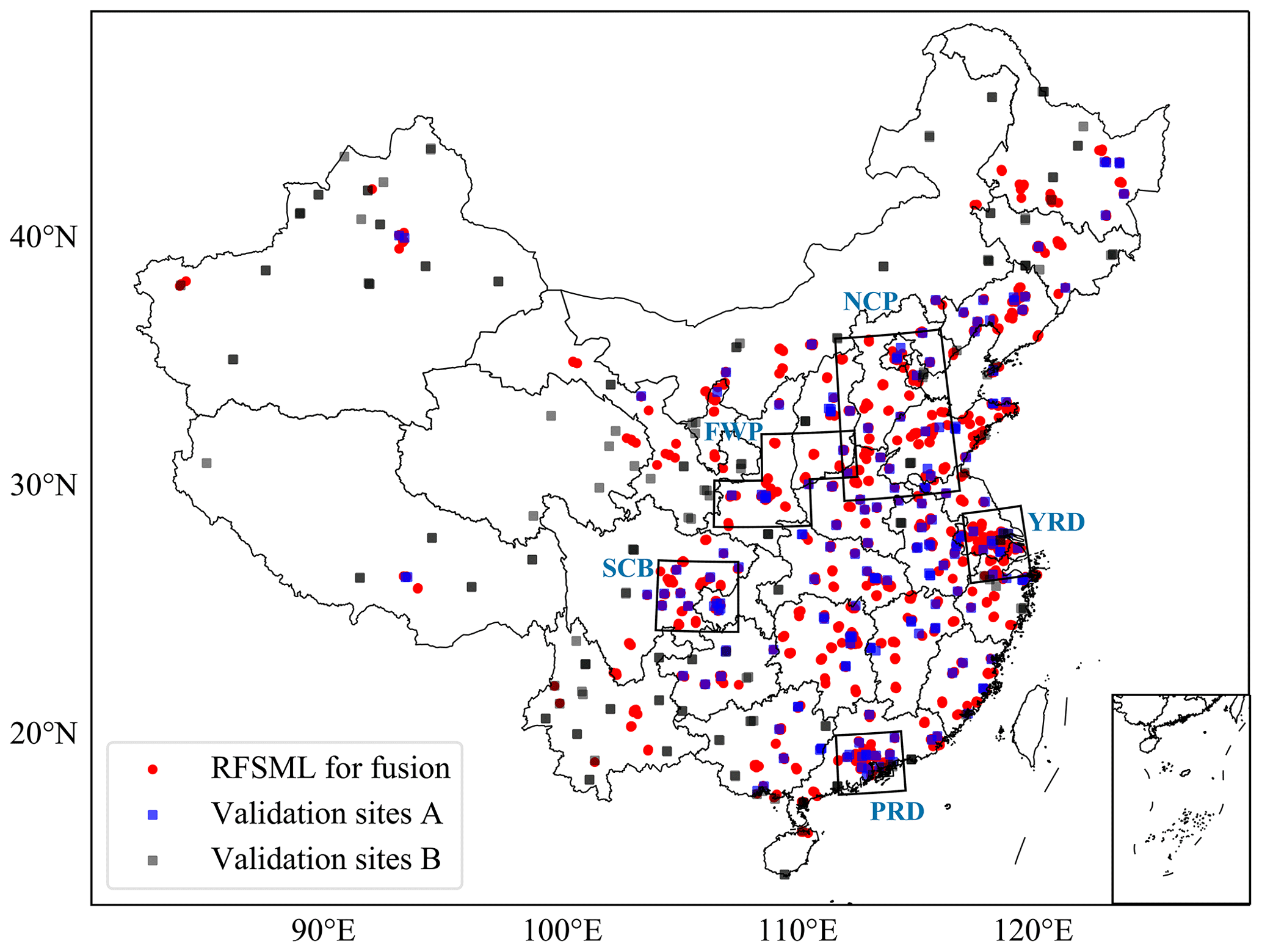
Figure 1 Distribution of air quality monitoring stations in the study area as of 2019. The black boxes represent the classification of five main megacity clusters used for the regional feature selection in RFSML. The RFSML predictions at these sites (represented by red dots) will be assimilated into the fused prediction. Independent evaluation will be carried out using observations from the blue and black rectangles.

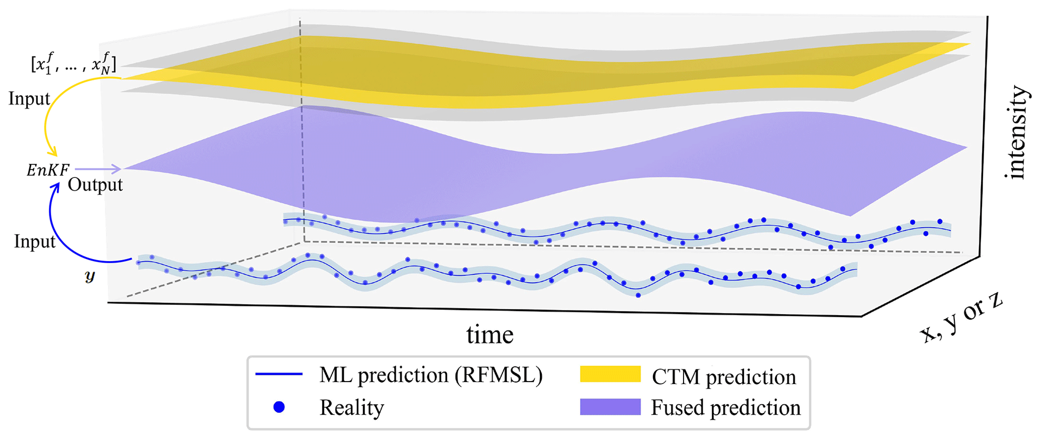
Figure 2 Framework of EnKF-based prediction fusion. The blue lines and their corresponding shaded regions represent the RFSML predictions and their uncertainty at the air quality monitoring stations, which are assumed to be very close to the actual PM_2.5 concentration values. The golden surface and its surrounding gray surfaces represent the CTM prediction and its uncertainty. The medium-slate-blue surface represents the fused prediction of the RFSML and CTM prediction. y and [${\mathit{x}}_{\mathrm{1}}^{\mathrm{f}},\mathrm{\dots },{\mathit{x}}_N^{\mathrm{f}}$] are the inputs of EnKF, which represent RFSML prediction and ensemble CTM prediction respectively.

2.2 EnKF-based prediction fusion

The proposed assimilation-based prediction fusion is illustrated in Fig. 2. This figure shows the time series of hypothetical ambient pollutant predictions from both machine learning models and pure CTMs along the spatial coordinates, which could be X, Y, or Z, without the loss of generality. The data-driven forecast using our RFSML system, indicated by the blue line, provided an accurate short-term forecast of the air pollutants that is very close to reality (blue dots), as validated in Fang et al. (2022) and as can also be seen in Fig. 3. However, they are only available at limited sites where observation stations are located as explained before. The dynamic variance was introduced in this study to describe the uncertainty of the RFSML results, as denoted by the light-blue shading. Unlike the data-driven forecast, the CTM provides predictions over the continuous 3D field (indicated by a gold curved surface), but it might contain unavoidable systematic bias. The Bayesian-theory-based assimilation methodology is used to calculate the most likely posterior (or the fused prediction) given the potential spread of two priors.

The specific sequential assimilation system that is used to combine the site-available RFSML prediction and CTM prediction is the EnKF that was originally proposed by Evensen (1994) and further corrected by Evensen (2004). Similar to other assimilation algorithms, this assimilation system fundamentally relies on the Bayesian theory for finding the optimal posterior that fits the two priors quantified by their covariance matrices (Evensen et al., 2022).

To begin with, ensemble chemical transport model predictions (N=32) are forwarded with perturbed emission inventories, as will be discussed in Sect. 2.4, as follows:

$$\begin{array}{}\text{(1)}& [{\mathit{x}}_{\mathrm{1}}^{\mathrm{f}},\mathrm{\dots },{\mathit{x}}_N^{\mathrm{f}}],\end{array}$$

where ${\overline{\mathit{x}}}^{\mathrm{f}}\in R^n$ equals the ensemble mean of ${\mathit{x}}_i^{\mathrm{f}}\in R^n$, and ${\mathbf{X}}^{\prime }\in R^{n\times N}$ calculates the perturbation of the ensemble predictions as

$$\begin{array}{}\text{(2)}& {\mathbf{X}}^{\prime }=[{\mathit{x}}_{\mathrm{1}}^{\mathrm{f}}-{\overline{\mathit{x}}}^{\mathrm{f}},\mathrm{\dots },{\mathit{x}}_N^{\mathrm{f}}-{\overline{\mathit{x}}}^{\mathrm{f}}],\end{array}$$

where N represents the ensemble number, while n denotes the gridded chemical transport model size. The spatial background covariance matrix of the CTM prediction $\mathbf{P}\in R^{n\times n}$ can be approximated using the ensemble perturbations via

$$\begin{array}{}\text{(3)}& \mathbf{P}={\displaystyle \frac{\mathrm{1}}{N-\mathrm{1}}}{\mathbf{X}}^{\prime }{{\mathbf{X}}^{\prime }}^{\text{T}}.\end{array}$$

The posterior forecast ${\mathit{x}}_{\mathrm{a}}^{\mathrm{f}}$ can then be fused according to the EnKF rules via

$$\begin{array}{}\text{(4)}& {\mathit{x}}_{\mathrm{a}}^{\mathrm{f}}={\overline{\mathit{x}}}^{\mathrm{f}}+\mathbf{K}(\mathit{y}-\mathcal{H}{\overline{\mathit{x}}}^{\mathrm{f}}),\end{array}$$

where y∈R^m represents the RFSML machine learning forecast from m=1074 sites, as will be explained in Sect. 2.3; $\mathcal{H}\in R^{n\times m}$ is the linear operator that selects the gridded CTM prediction into the site-available machine learning forecast space; and K denotes the Kalman gain, which can be calculated as follows:

$$\begin{array}{}\text{(5)}& \mathbf{K}=\mathbf{P}{\mathcal{H}}^{\text{T}}(\mathcal{H}\mathbf{P}{\mathcal{H}}^{\text{T}}+\mathbf{O}{)}^{-\mathrm{1}},\end{array}$$

where $\mathbf{O}\in R^{m\times m}$ is the error covariance matrix of the machine learning forecast y, as will be illustrated in Sect. 2.3.

The classic EnKF has limitations such as its dependence on the relatively small ensemble number (N) compared to a high number of model dimensions (n) to estimate background error covariance P dynamics (Houtekamer and Mitchell, 2001). To cut off those spurious spatial correlations in P, the most representative distance-dependent localization scheme (Lei and Anderson, 2014) is used. The localization is performed by multiplying a local support L via a Schur product as follows:

$$\begin{array}{}\text{(6)}& {\displaystyle }{\mathbf{P}}^{\text{local}}=\mathbf{P}\circ \mathbf{L}\text{(7)}& {\displaystyle }\begin{array}{rl}& {\mathbf{L}}_{i,j}=\\ & \left\{\begin{array}{cc}\mathrm{1}-{\displaystyle \frac{\mathrm{5}}{\mathrm{3}}}{\mathbf{S}}_{i,j}^{\mathrm{2}}+{\displaystyle \frac{\mathrm{5}}{\mathrm{8}}}{\mathbf{S}}_{i,j}^{\mathrm{3}}+{\displaystyle \frac{\mathrm{1}}{\mathrm{2}}}{\mathbf{S}}_{i,j}^{\mathrm{4}}-{\displaystyle \frac{\mathrm{1}}{\mathrm{4}}}{\mathbf{S}}_{i,j}^{\mathrm{5}},& {\mathbf{S}}_{i,j}<\mathrm{1}\\ -\frac{\mathrm{2}}{\mathrm{3}}{\mathbf{S}}_{i,j}^{-\mathrm{1}}+\mathrm{4}-\mathrm{5}{\mathbf{S}}_{i,j}+\frac{\mathrm{5}}{\mathrm{3}}{\mathbf{S}}_{i,j}^{\mathrm{2}}+\frac{\mathrm{5}}{\mathrm{8}}{\mathbf{S}}_{i,j}^{\mathrm{3}}-\frac{\mathrm{1}}{\mathrm{2}}{\mathbf{S}}_{i,j}^{\mathrm{4}}+\frac{\mathrm{1}}{\mathrm{12}}{\mathbf{S}}_{i,j}^{\mathrm{5}},& \mathrm{1}\le {\mathbf{S}}_{i,j}<\mathrm{2}\\ \mathrm{0},& {\mathbf{S}}_{i,j}\ge \mathrm{2}\end{array}\right.\end{array}\text{(8)}& {\displaystyle }{\mathbf{S}}_{i,j}={\displaystyle \frac{{\mathbf{D}}_{i,j}}{L_{\mathrm{thres}}}},\end{array}$$

where D_i,j represents the spatial distance between the grid cell i and j, while L_thres is the localization distance threshold. The individual elements of the local support L can be calculated using Eqs. (7) and (8). The correlation L_i,j declines as the distance increases. The shorter distance threshold equals the greater descent rate. In this study, it was empirically set as 300 km, which was tested to give the optimal performance.

2.3 RFSML prediction and uncertainty

Approximately 1500 air quality monitoring stations are present over China that provide hourly ambient pollutant measurements up to 2019 as shown in Fig. 1. Recently, the regional feature selection-based machine learning forecast system (RFSML) was successfully developed for short-term (with a horizon up to 24 h) air quality predictions. The common machine learning prediction process involves several steps. Firstly, it requires data collection of PM_2.5 observations and datasets. Next, data interpolation should be conducted to address missing values in the original dataset. Following that, an appropriate machine learning model must be selected. Additionally, the continuous data time series should be reformed into the required input structure. Then, the model is repeatedly trained to determine optimal hyperparameters. Finally, predictions can be made using the trained model. In addition to these procedures, the RFSML utilized the SAGE ensemble to obtain the optimal input feature subsets instead of using all related features. The total national air quality monitoring stations were divided into six regions. Using a computationally efficient SAGE ensemble selection, we identified the top three significant features for each region, as outlined in the Supplement Table S1 (Table 6; Fang et al., 2022). Given the regional key feature subset ${\mathit{a}}_s=\mathit{\{}{a}_{\mathrm{1}},a_{\mathrm{2}},\mathrm{\dots },a_s\mathit{\}}$, the RFSML can be described mathematically as follows:

$$\begin{array}{}\text{(9)}& \begin{array}{rl}{\widehat{y}}_{t+h}& =\mathcal{F}(a_{\mathrm{1}}^{t-t_{\mathrm{p}}+\mathrm{1}},\mathrm{\cdots },a_{\mathrm{1}}^t,a_{\mathrm{2}}^{t-t_{\mathrm{p}}+\mathrm{1}},\mathrm{\cdots },a_{\mathrm{2}}^t,\mathrm{\cdots },\\ & \mathrm{\cdots },a_s^{t-t_{\mathrm{p}}+\mathrm{1}},\mathrm{\cdots },a_s^t),\end{array}\end{array}$$

where at any instant t, the input vector storing s=3 individual selected features over the previous t_p = 9 h is utilized to forecast the target PM_2.5 concentrations $\widehat{y}$ with a prediction horizon of h h. The choice of t_p=9 h is obtained on the basis of the auto-correlation and partial auto-correlation analysis. The forecast predictor F represents the machine learning model. In RFSML, three machine learning models, namely random forest, gradient boosting, and multi-layer perceptron (MLP), are employed. The prediction results obtained from MLP are directly utilized as this work's RFSML prediction. A highlight in RFSML was use of the SAGE ensemble algorithm to select the regional key features, which resulted in remarkable improvements in the forecast effeciency (Fang et al., 2022).

These high-quality predictions were available at 1262 stations (denoted as red dots and blue rectangles in Fig. 1), and 188 were skipped because of the high missing data rate in the data interpolation period (January 2018 to October 2019). Details concerning the strict data quality control can be found in Fang et al. (2022). These stations however still contain valuable measurements for validation. For this study, the 188 stations that were skipped in the RFSML model training were used for validating our fused prediction; they are referred to as validation sites B and marked as black rectangles in Fig. 1.

Meanwhile, these 188 validation sites B are not evenly distributed over the entire modeling domain, as can be seen in Fig. 1. To fully evaluate the forecasting ability of the proposed gridded prediction system, an additional 188 sites were randomly selected from the 1262 RFSML stations and used for cross-validations. They are referred to as validation sites A, as shown in Fig. 1. Conclusively, the RFSML predictions at 1074 air quality monitoring stations (red dots) are used as one prior (y) for the fused prediction, which is then compared with the measurements at 376 stations (blue rectangles and black rectangles) for validation, as can be seen in Fig. 1. Snapshots of our RFSML predictions at 1074 stations for assimilation are available in Fig. 6a–c, which captured the spatial variations in the PM_2.5 exactly, as shown in Fig. S1 in the Supplement. Our RFSML is capable of providing the operational air quality prediction with a maximum horizon of 24 h. The RFSML prediction results used in this study are directly acquired from our last work (Fang et al., 2022).

As aforementioned, the error covariance matrix of the RFSML forecast (O) is the essential input for Kalman gain calculation in Eq. (5). It governs the weight of the y prior in the optimization by describing its potential distribution. The errors in the RFSML predictions were assumed to be spatially independent, and hence O was diagonal. The RFSML errors are not only varied in different stations but also dynamically varied in a given site. The typical method is shown in Fig. 3a, presenting the relationship between observations and RFSML prediction at a random site. The RFSML-predicted PM_2.5 values were relatively close to the observations. Moreover, it presented high errors under severely polluted scenarios. To explore the variations in the RFSML uncertainties, the samples shown in Fig. 3a were evenly divided into 10 collections (indicated by the dashed gray line) based on the observation values. The mean values and root mean square errors (RMSEs) of the 10 sample collections are plotted in Fig. 3b, and their relationship was described using a linear function (solid blue line). Instead of characterizing the error using a fixed value, the linear function was used to quantify the RFSML prediction error at the given station. The individual diagonal elements in O storing the square of the dynamic RFSML prediction error were then calculated by repeating the above calculation.

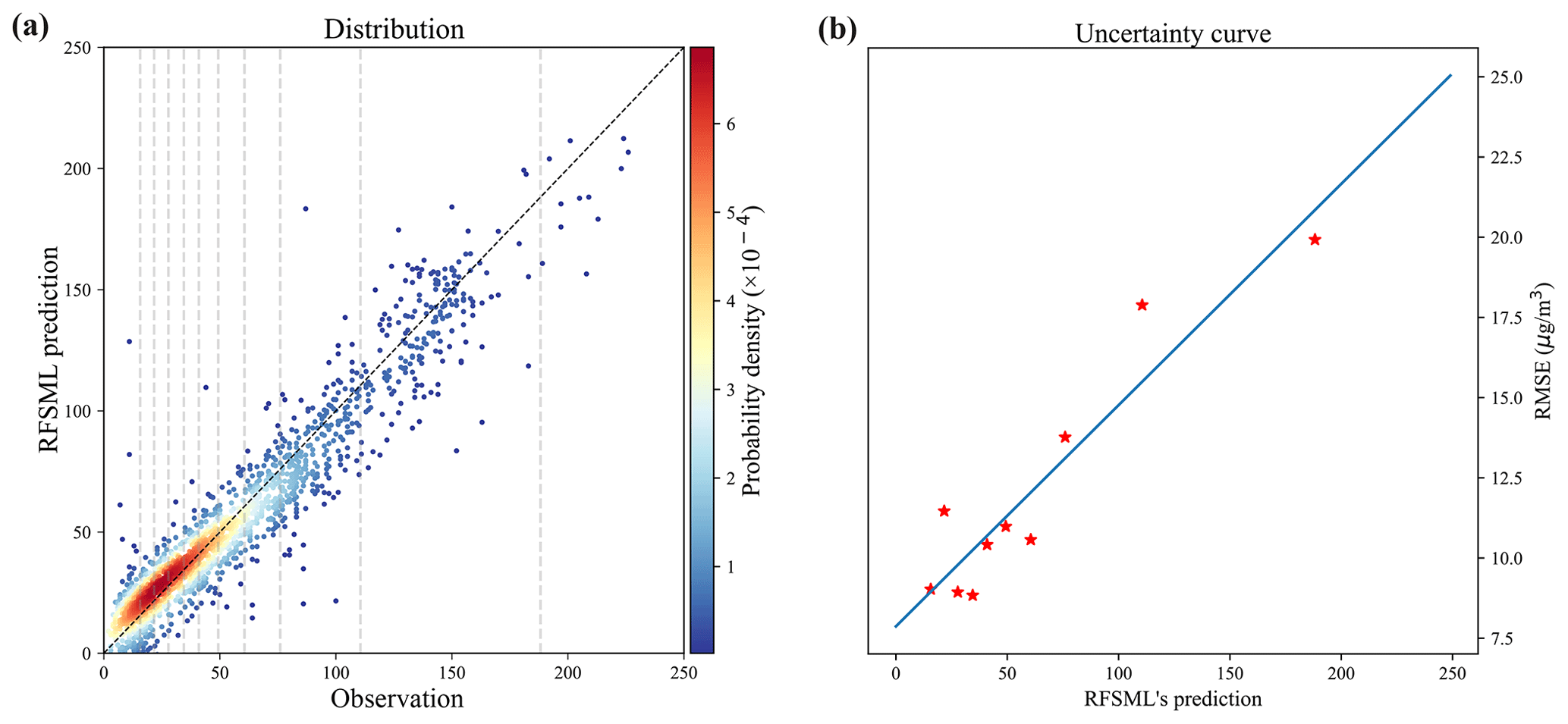
Figure 3 Dynamic uncertainty of the RFSML prediction at a random air quality station. Panel (a) is the distribution of the observation and RFSML prediction 6 h in advance. Panel (b) shows the linear fit of the average RFSML prediction and RMSE. The averages in panel (b) correspond to the intervals depicted in panel (a).

2.4  CTM prediction

The short-term CTM prediction used for gridded prediction fusion in this study was from the GEOS-Chem v13.1.0 (https://doi.org/10.5281/zenodo.4984436, The International GEOS-Chem User Community, 2021) in a nested-grid simulation. It takes the global simulation with a horizontal resolution of 2^∘ latitude by 2.5^∘ longitude as the boundary condition. The nested modeling domain of China (0–55^∘ N, 70–140^∘ E) has a horizontal resolution of 0.5^∘ latitude by 0.625^∘ longitude and 47 vertical layers. This version had fully coupled aerosol–ozone–NO_x–hydrocarbon chemistry representation (Park et al., 2004; Dang and Liao, 2019). In this study, GEOS-Chem was driven by the archived Modern Era Retrospective analysis for Research and Applications, version 2 (MERRA-2) meteorological fields (Gelaro et al., 2017). Notably, the reanalysis meteorology product was temporally used for testing our prediction fusion methodology. For the CTM prediction in practice, the operational meteorology forecast is the essence, e.g., the GEOS-CF (Keller et al., 2021) and WRF-GC system (Lin et al., 2020). Note that the CTM results utilized in this work remain consistent regardless of changes in the forecast horizon. The global anthropogenic emission inventory used in this study was the Global anthropogenic emissions from the Community Emissions Data System (CEDS) inventory (Hoesly et al., 2018), which primarily contains aerosol, aerosol precursor, and reactive compounds. The monthly anthropogenic emission inventory for China is the Multi-resolution Emission Inventory for China (MEIC; http://www.meicmodel.org, last access: 13 July 2023) (Zheng et al., 2018). The MEIC utilized here was the 2017 collection, which is the latest version. Several natural emission sources were also included in the model that can dynamically respond to the meteorological conditions, such as NO_x emissions during lightning (Murray et al., 2012) and biogenic emissions which are computed online using MEGAN2.1 (Model of Emissions of Gases and Aerosols from Nature version 2.1; Guenther et al., 2012). To achieve the successful operation of GEOS-Chem, a 3-month spin-up simulation was carried out before testing the 2019 winter PM_2.5 prediction. The PM_2.5 concentrations were calculated as the sum of the concentrations of the sulfate, nitrate, ammonium, black carbon, and organic carbon in this study.

2.4.1 CTM prediction covariance

The uncertainty in the GEOS-Chem prediction is initially attributed to the errors in the emission inventories. It is assumed to be compensated for using a spatially varying tuning factor similar to the approach in related work (Di Tomaso et al., 2017; Jin et al., 2018), as follows:

$$\begin{array}{}\text{(10)}& {\mathit{f}}^{\text{true}}\left(i\right)={\mathit{f}}_b\left(i\right)\cdot \mathit{\alpha }\left(i\right),\end{array}$$

where f_b(i) denotes the aerosol emission rate in the given grid cell i from the MEIC, and f^true(i) represents the true value. The α values are defined to be random variables with a mean of 1.0 and a standard deviation σ_α=0.2. This empirical value was found to provide sufficient freedom for resolving the observation-minus-simulation errors to a large extent. A background covariance B_α was formulated as a product of the constant standard deviation and a spatial correlation matrix C:

$$\begin{array}{}\text{(11)}& {\mathbf{B}}_{\mathit{\alpha }}(i,j)={\mathit{\sigma }}_{\mathit{\alpha }}\cdot \mathbf{C}(i,j),\end{array}$$

where C(i,j) represents a distance-based spatial correlation between two αs in the grid cell i and j and is defined as

$$\begin{array}{}\text{(12)}& \mathbf{C}(i,j)=e^{-(d_{i,j}/l{)}^{\mathrm{2}}/\mathrm{2}},\end{array}$$

where d_i,j represents the distance between two grid cells i and j. Here, l denotes the correlation length scale, which controls the spatial variability freedom of the αs. A small l means more errors in fine scale could be resolved using the assimilation, which however requires more ensemble runs to represent the model realization from emission to simulation, as will be explained later. An empirical parameter l=300 km used in EnKF to cut off the dust emission that has a rapid spatial variability was also considered in this study.

With B_α that describes the potential spread of the true emission situation, the ensemble emission inventory $[{\mathit{f}}_{\mathrm{1}},\mathrm{\dots },{\mathit{f}}_N]$ could then be generated randomly. They will then be input into our GEOS-Chem model ℳ for ensemble PM_2.5 predictions in Eq. (1) via

$$\begin{array}{}\text{(13)}& [{\mathit{x}}_{\mathrm{1}}^{\mathrm{f}},\mathrm{\dots },{\mathit{x}}_N^{\mathrm{f}}]=\left[\mathcal{M}\right({\mathit{f}}_{\mathrm{1}}),\mathrm{\dots },\mathcal{M}({\mathit{f}}_N\left)\right].\end{array}$$

2.4.2 Covariance inflation

The perturbed emission inventories could resolve the deficiencies in the model prediction effectively, as will be discussed in Sect. 3, by feeding the site-available RFSML result. However, the posterior forecast error occasionally remained at high values, especially when the prior CTM severely underestimated the pollution levels. This is evident in Fig. 4. Panel (a) shows the times series plot of prediction from RFSML with the uncertainty, mean CTM predictions with its uncertainty, PM_2.5 concentration measurements, and fused result at a station labeled as 1063A. Note that the mean and uncertainty (standard deviation) of the CTM are calculated based on the ensemble CTM simulations, which could be found in Fig. S2a as well. The difference between the fused prediction (sky-blue line) and observations (red stars) is not resolved steadily, especially in the red marked regions. The uncertainty quantified by the CTM spread (silver shading) is far less than the RFSML uncertainty (blue shading). Therefore, the prior CTM prediction was weighted more highly than the prior of RFSML in the assimilation. This resulted in a posterior prediction at a level similar to that of the mean ensemble result (black dot) and deviated considerably from the RFSML prediction (blue line). This could be attributed to the fact that the perturbed MEIC emission uncertainty only partially accounts for the simulation-minus-observation error in CTM prediction. However, the unconsidered error caused by meteorology, deposition, and other processes could also contribute to the simulation-minus-observation error.

To compensate for these inevitable errors in the CTM uncertainty and avoid the assimilation divergence, covariance inflation was designed. The basic idea was to amplify the ensemble perturbations while maintaining the mean via

$$\begin{array}{}\text{(14)}& {\mathit{x}}_i^{\text{inflate}}\left(j\right)=\overline{\mathit{x}}\left(j\right)+\mathit{\beta }\left[{\mathit{x}}_i\right(j)-\overline{\mathit{x}}(j\left)\right],\end{array}$$

where x_i(j) represents the original prediction from the ensemble i at grid cell j, while ${\mathit{x}}_i^{\text{inflate}}$ denotes the inflated one, and β is the inflation factor for amplifying the ensemble perturbation with respect to the ensemble mean $\overline{\mathit{x}}\left(j\right)$, which is defined as follows:

$$\begin{array}{}\text{(15)}& \mathit{\beta }=\mathrm{15}\cdot e^{-\left(\overline{\mathit{x}}\right(j)/\mathrm{5})}+\mathrm{1.5}.\end{array}$$

As the ensemble mean increase, the inflation factor declines smoothly from a maximum of 16.5 to a minimum of 1.5 as shown in Fig. 4c. The spread of the resampled ensemble CTMs is available in the Supplement Fig. S2b. Higher inflation was set for these low-value predictions to compensate for the uncertainty raised by meteorology or other transport processes. The posterior prediction could subsequently be calculated with the inflated covariance.

Figure 4b shows the time series of the uncertainty of the resampled ensemble members, presenting a much wider spread compared to the original ones in panel (a). This effectively avoids assimilation divergence and allows the posterior prediction to be nudged toward RFSML. Overall improvement on gridded prediction against independent measurements will be discussed in Sect. 3.

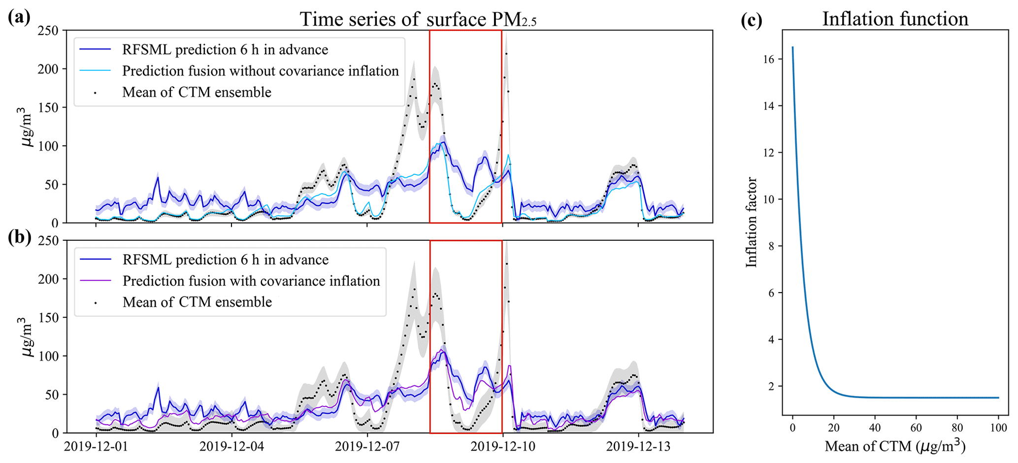
Figure 4 Panels (a) and (b) are the time series of an environmental monitoring station (latitude: 40.98^∘ N, longitude: 117.95^∘ E) in Chengde, Hebei Province. RFSML prediction is available at this station and will be assimilated. The solid medium-blue line, solid deep-sky-blue line, solid dark-violet line, and black dot represent the RFSML prediction, prediction fusion without covariance inflation, prediction fusion with covariance inflation, and mean ensemble CTM predictions respectively. The silver and blue shading represents the uncertainty of the CTM and RFSML respectively. Panel (c) is the inflation function.

2.5 Spatial interpolation benchmark: the Cressman interpolation

Interpolating data from observational stations to regular grid cells is also a hot topic in the geoscience (Yu et al., 2011). Many deterministic and geospatial tools for spatial interpolation have been developed, such as the Cressman interpolation (Cressman, 1959), kriging interpolation (Oliver and Webster, 1990; Stein, 1999), and inverse distance weighting (Bartier and Keller, 1996). These methods can transfer the site-available RFSML prediction into the continuous 3D field product alternatively. All these methods are based on the assumption that the weight is inversely proportional to the distance between the predicted location and the sampling location (Lu and Wong, 2008). Therefore, they are relatively simple and efficient in computation compared to our proposed prediction fusion method, which relies on the ensemble CTMs to represent the spatial covariance statistics.

In this work, these popular tools including ordinary kriging interpolation, the Cressman interpolation, and inverse distance weighting were also tested to interpolate our site-available RFSML prediction in order to obtain a gridded one. They are served as the benchmark for comparing against our proposed assimilation-based fusion method. To ensure a fair comparison, the statistical interpolation methods were performed based on the RFSML prediction at 1074 sites which were used for our assimilation-based fusion. However, they failed to forecast the spatial pattern of the PM_2.5 concentration either on the national scale or on a fine scale. Of the three, the Cressman interpolation provided the most optimal results. Snapshots of the prediction interpolation are shown in panels (a), (b), and (c) in Fig. 5, with a scaling radius of 3, 5, and 10^∘respectively. The typical limitations of using these distance-weighted methods can be clearly observed in the figure. While parts of the PM_2.5 spatial pattern were captured with the hottest spot in the North China Plain using the smallest search radius in panel (a), it failed to obtain the full gridded prediction as the air quality monitoring stations are sparsely distributed, especially in the western areas. However, when using a large scaling radius, most of the spatial dynamics are lost with a huge discrepancy against the independent measurements (indicated by colored circles) in panel (c). Therefore, distance-weighted methods cannot satisfy the motivation for obtaining a 3D continuous prediction starting from the site-available machine learning forecast. It is worth noting that the interpolation method is computationally less expensive than the fusion method, and it can be a powerful tool for gridded prediction when there are plenty of ground observations available.

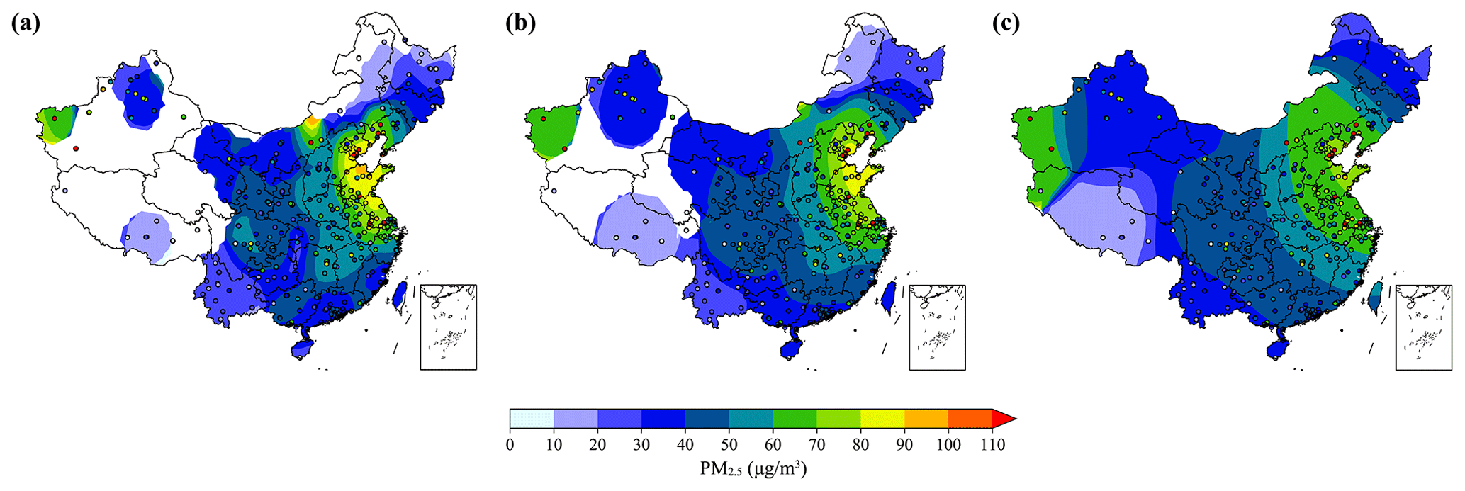
Figure 5 Snapshots of the distribution of the PM_2.5 concentration forecasts and observations on 30 October 2019 at 16:00:00 (UTC). Panels (a), (b), and (c) represent the Cressman interpolation of the RFSML (6 h in advance) predictions with a scaling radius of 3, 5, and 10^∘. The colored circles imply the independent observations from 376 ground stations which are not used as a source of interpolation.

3 Results and discussion

The effectiveness of our gridded prediction approach, which combines machine learning and CTM prediction using EnKF, was thoroughly assessed. First, the performance of the CTM was evaluated and discussed in Sect. 3.1. Next, the impressive skill of our proposed approach in terms of time series prediction at single stations was demonstrated in Sect. 3.2, highlighting the importance of using covariance inflation. Finally, the overall spatial performance of the fused prediction against independent observations was evaluated over the entire test period in Sect. 3.3. To assess the performance, we used RMSE, mean absolute error (MAE), and Pearson correlation coefficient (R) metrics, whose formulas are provided in Formulas (S2)–(S4) of the Supplement.

3.1 Pure CTM prediction

An ensemble of 32 CTM predictions with the disturbed MEIC was forwarded to quantify the spatial covariance statistic of the PM_2.5 prediction as discussed in Sect. 2.4. In addition, a base run driven by the default MEIC was performed over the test period (2019 winter) to verify the prediction skill of the pure CTM. This run served as the benchmark for validating our fused prediction.

The overall evaluation results of the CTM prediction in terms of RMSE and MAE over the test period are shown in Fig. 8. Although the CTM can reproduce the PM_2.5 spatial and temporal variation to a larger extent, as will be discussed in Sect. 3.2 and 3.3 in detail, a noticeable difference in PM_2.5 intensity exists, resulting in relatively high RMSE and MAE. In severely polluted regions such as the NCP and FWP, the RMSE and MAE were particularly high, reaching values as high as 42.8 and 29.7 µg m⁻³ and 47.0 and 32.8 µg m⁻³ respectively. Moreover, the significant overestimation in the SCB region contributes to the high RMSE and MAE (53.1 and 42.6 µg m⁻³), which are consistent with the findings of Li et al. (2016b). Model validation of the CTM is shown in the Supplement Fig. S3, with a normalized mean bias (NMB) of −6.87 % over the entire test period. Details concerning improvements of the proposed fused prediction over the pure CTM will be given in Sect. 3.3.

3.2  Time series of single monitoring station

One of the 376 environmental monitoring stations used for independent validation, station 1812A (34.65^∘ N, 112.39^∘ E), was selected as a typical example for the time series discussion. This station was used to illustrate the typical results that were observed at other validating sites. Panels (a) and (b) in Fig. 6 show the pure CTM prediction and fused forecasts (6 and 18 h in advance respectively) against the independent PM_2.5. While the CTM captured the temporal dynamics at station 1812A in general, there were significant differences in magnitude at times. By assimilating the spatial pattern from the site-available RFSML result, the fused gridded prediction outperformed the purely CTM prediction significantly. Notably, the optimal result was obtained with covariance inflation implemented. The posterior prediction with covariance inflation performed better, especially in low-value PM_2.5 situations, as discussed in Sect. 2.4.2. To further highlight the superior forecast skill, we present the distributions of both prediction fusion methods and ground observations for a 6 h prediction horizon in the Supplement Fig. S5. The results clearly indicate that the prediction fusions align closely with the ground observations and that the prediction fusion with covariance inflation effectively addresses the underestimation issue present in the prediction fusion without covariance inflation.

The benefit of the covariance inflation is highlighted when the RFSML forecast is fused for longer prediction horizons, as shown in panel (b) (18 h). This is because the dynamic error of RFSML grows steadily as the prediction length increases (Fang et al., 2022). Without using covariance inflation, the assimilation algorithm would rely more on the CTM than on RFSML, resulting in a forecast that stays closer to the CTM prior. A similar outcome can be observed in the Supplement Fig. S4, which shows the time series diagram of the same station for forecast horizons of 12 and 24 h. However, there is one exception around 23 December 2019 (UTC), where CTM overestimates the PM_2.5 concentrations, while prediction fusion all underestimates it. This discrepancy is mainly due to the abnormally low prediction values from the RFSML at nearby sites. In general, the proposed prediction fusion exhibits significant advantages over CTM, and the adopted covariance localization effectively prevents the assimilation divergence and further improves the gridded prediction fusion.

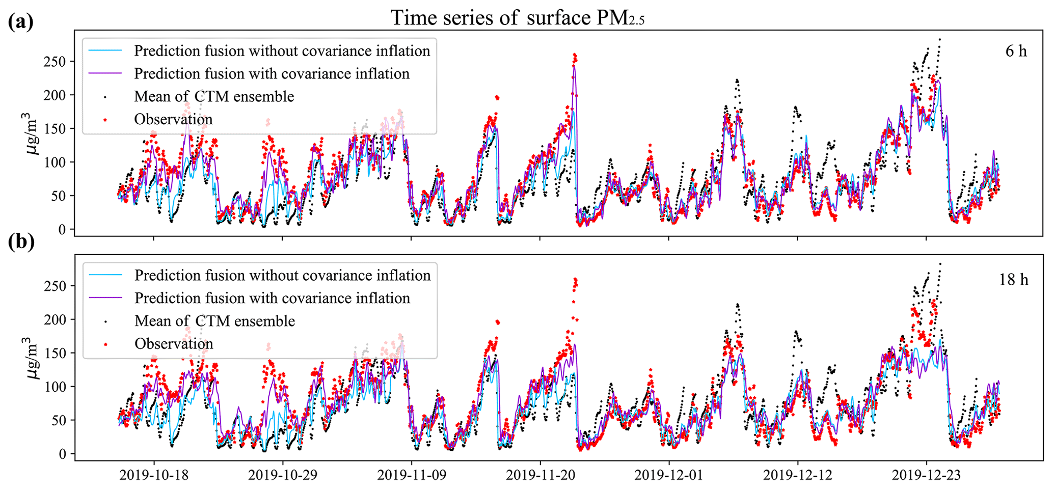
Figure 6 Time series of an environmental monitoring station (latitude: 34.65^∘ N, longitude: 112.39^∘ E) in Luoyang, Henan Province. This station is one of the validation set. The solid deep-sky-blue line, solid dark-violet line, red star, and black dot represent prediction fusion without covariance inflation, prediction fusion with covariance inflation, ground observation, and mean ensemble CTM predictions respectively. Panels (a) and (b) represent forecasts 6 and 18 h ahead respectively.

3.3 Spatial forecast

Figure 7 depicts the spatial distribution of the fused predictions (panels g–i) and the ones using extra covariance inflation (panels j–l) against the independent PM_2.5 measurements at three randomly selected tested instants. Those two gridded posteriors were obtained via fusing the site-available RFSML in panels (a)–(c) and CTM prediction in panels (d)–(f). The proposed fused prediction consistently exhibits improvements in the spatial pattern compared to the pure CTM. Specifically, the CTM underestimated the PM_2.5 pollution over the NCP region at the first (red box in panel d) and third instants (red box in panel f). The underestimation was partially relieved by assimilating the RFSML prediction (see panels g and i). The CTM's overestimations in the SCB (panel e) and the south of China (panel f) were also reduced to a great extent by the proposed prediction fusion (see panels h and i). When severe underestimation occurred in northern China (green box in panels), especially in Xinjiang Province, assimilating only the RFSML prediction was not sufficient to correct it. However, the application of covariance inflation effectively resolved the underestimation in the fused predictions, as shown in panels (j), (k), and (l) (green box). Overall, these results demonstrate the potential of our proposed prediction fusion approach to improving the accuracy of PM_2.5 predictions, especially in regions with complex and heterogeneous air quality patterns.

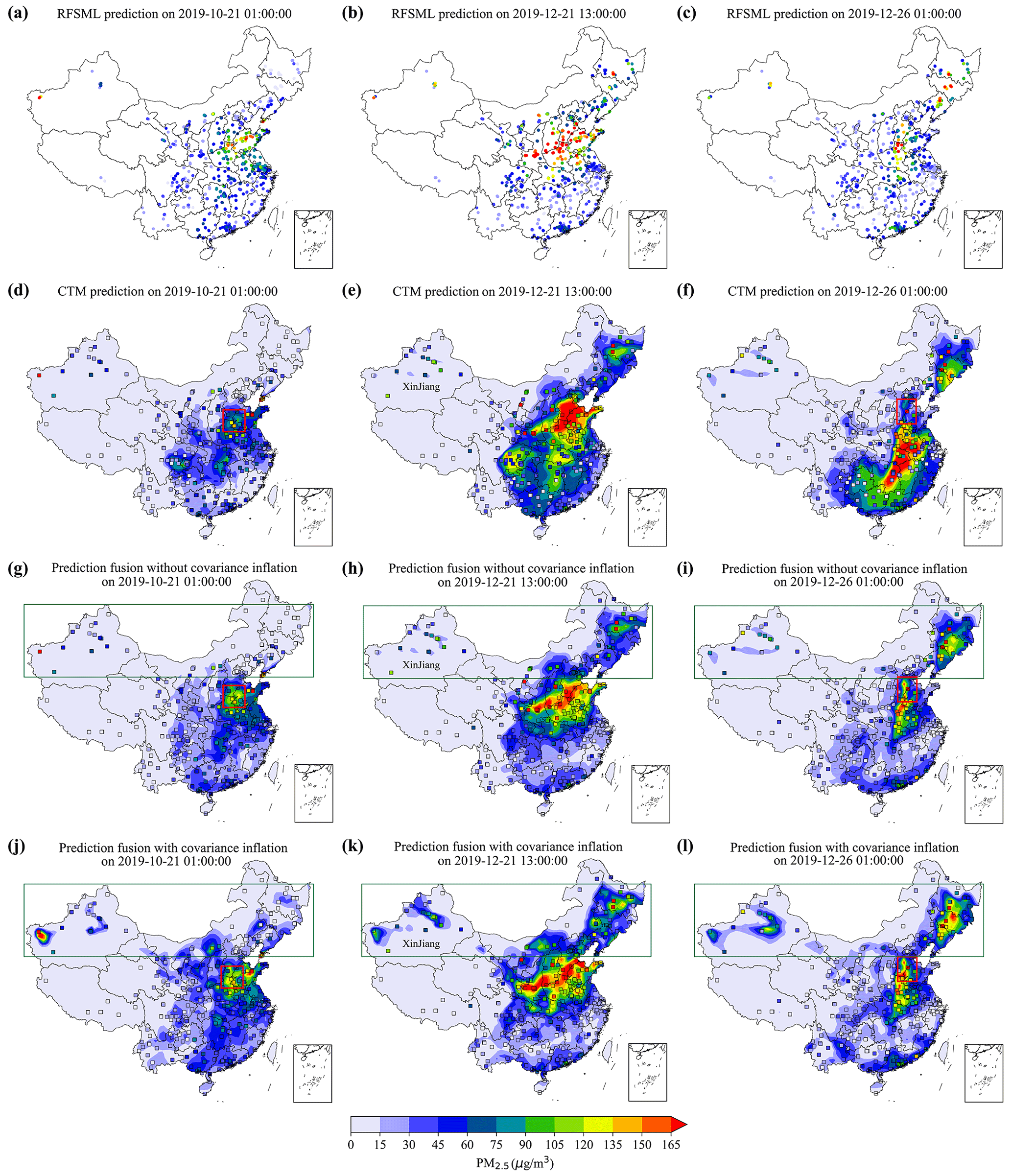
Figure 7 Snapshots of PM_2.5 forecast 6 h in advance at three instants (each column indicates the same moment). Panels (a)–(c) show the RFSML predictions (colored dots) at 1074 air quality stations. Panels (d)–(f) show the CTM prediction and the ground observation (colored dots). Panels (g)–(l) show the prediction fusion (without and with covariance inflation) results and the actual results (colored squares) from 376 evaluation stations.

In summary, the fused prediction obtained through assimilating the high-quality RFSML prediction could effectively improve CTM spatial variability prediction. Additionally, the covariance inflation can further enhance the performance of the prediction fusion, especially in places with severe underestimation. This is mainly because the perturbed MEIC emission only partially accounts for the simulation-minus-observation error. The error caused by meteorology, deposition, and other processes should also be taken into account, as has been done in our proposed covariance inflation.

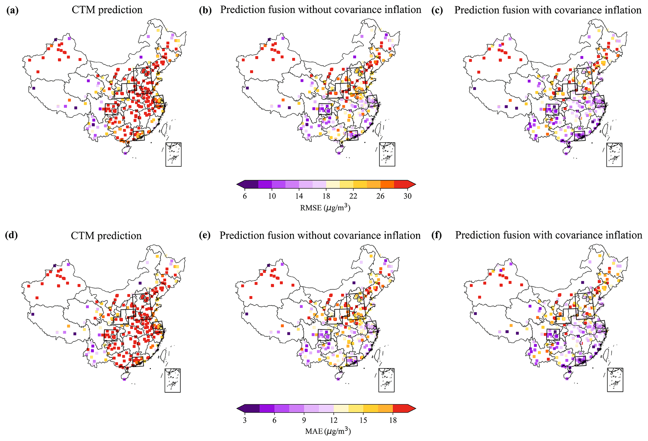
Figure 8 Spatial statistics of CTM, prediction fusion without covariance inflation, and prediction fusion with covariance inflation. Panels (a)–(c) and panels (d)–(f) represent statistical results of RMSE and MAE respectively. The results are based on prediction 6 h in advance.

Overall, the EnKF-based prediction fusion approach showed superior performance compared to the CTM in most of the validation stations, as indicated by the lower RMSE and MAE values shown in Fig. 8. However, there were a few sites where the improvements were limited, such as in Xinjiang Province, which could be attributed to the lack of nearby RFSML sites for assimilation. The fused prediction with covariance inflation demonstrated even further improvement in prediction skill, particularly in areas with sufficient RFSML sites for assimilation, which were mainly located in the five major megacity clusters (indicated by the black boxes in Fig. 8).

To clearly visualize the benefit of using the EnKF-based prediction fusion method and covariance inflation, we present a modified Taylor diagram (Taylor, 2005) in Fig. 9, which shows the RMSE and R of the CTM and our fused prediction over the five clusters simultaneously. These metrics are calculated with respect to the independent air quality monitoring sites in the region. In terms of the Pearson correlation coefficient, the SCB shows the best predictability among the regions, while the PRD has the poorest performance. The smallest R value of the PRD can be attributed to both the smallest R value of RFSML and CTM predictions. However, no significant differences were observed in the predictive performance of these regions. Regarding the root mean square error (RMSE), the NCP and FWP exhibited the largest values. This outcome can be attributed to the fact that the NCP and FWP are located in the northern region of China, where the frequency of pollution days is higher due to adverse meteorological conditions and high emissions during winter. It should be noted that the RMSE metric is directly influenced by the atmospheric pollution levels, wherein higher PM_2.5 concentrations tend to yield larger RMSE.

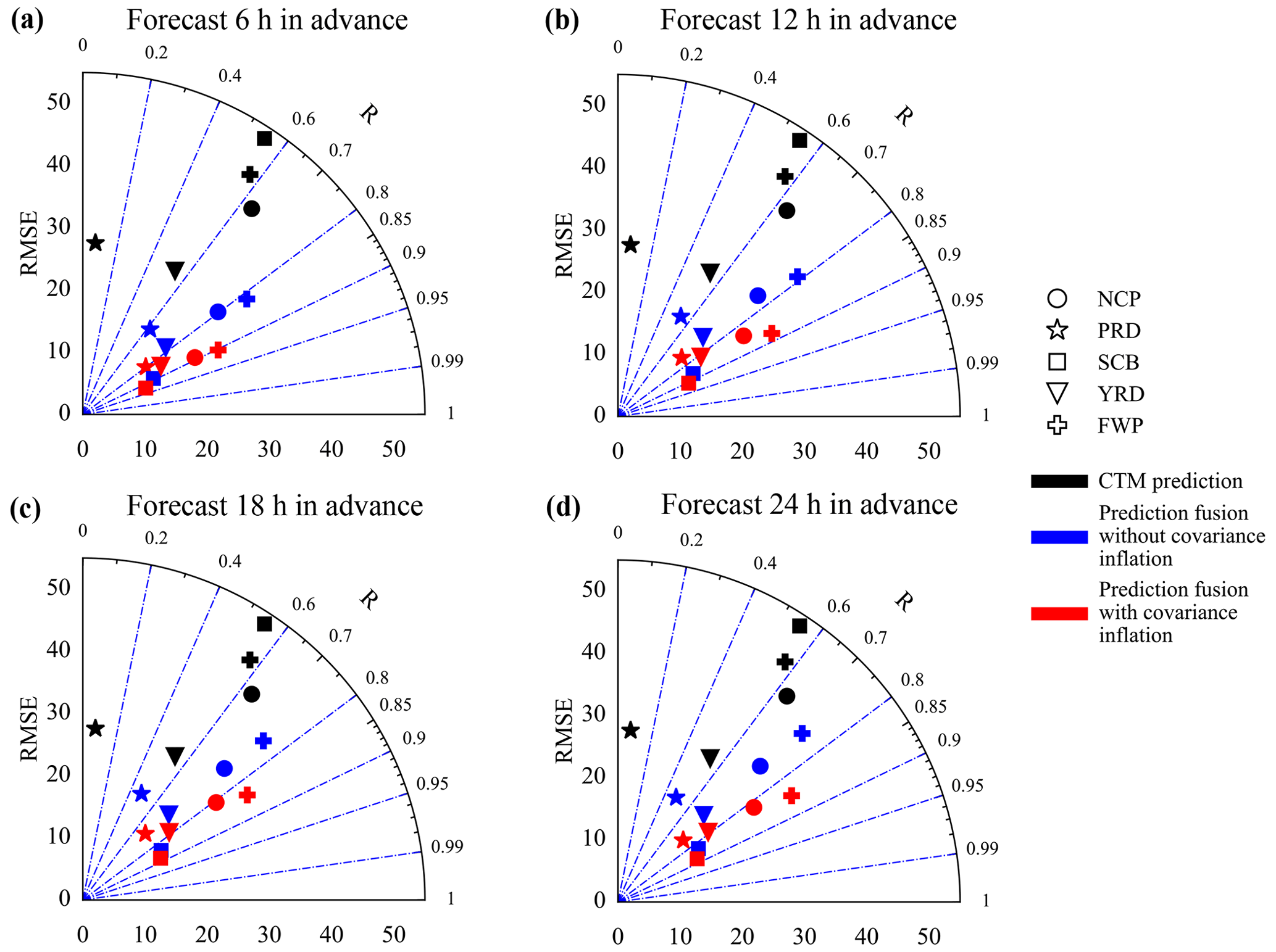
Figure 9 A modified Taylor diagram that illustrates RMSE and R together. The NCP, PRD, SCB, YRD, and FWP were represented by the circle, star, square, triangle, plus symbol, and diamond respectively. Black, blue, and red indicate results from CTM, prediction fusion without covariance inflation, and prediction fusion with covariance inflation respectively. The panels from top left to bottom right are forecasts 6, 12, 18, and 24 h ahead.

The improvement in prediction skill using our prediction fusion method compared to the pure CTM prediction is consistent across all five regions and various prediction horizons (6, 12, 18, and 24 h). For example, in panel (a), the CTM has the worst prediction in terms of R (<0.1) in the PRD region, but it increases to 0.62 when the RFSML forecast is assimilated and further increases to 0.85 when covariance inflation is implemented. In terms of the RMSE, the most remarkable improvement is obtained in the SCB region. Our EnKF-based fusion reduced the RMSE from 43 to 12.73 µg m⁻³ and 10.97 µg m⁻³ (with covariance inflation). This is a considerable improvement and can be attributed to the densely distributed RFSML prediction sites in the region, as can be seen in Fig. 1. Note that our fused prediction skill also generally declines with an increase in prediction length following the RFSML. Therefore, prediction fusion with a longer forecasting horizon (>24 h) was not carried out. Thus, the prediction fusion method has much better prediction performance than CTM, and covariance inflation can further enhance this advantage in all the tested predicting horizons.

To further showcase the robustness of the proposed prediction fusion approach, we conducted testing for a less polluted month (April 2020) using prediction horizons of 6 and 18 h. The overall performance of each region is illustrated in the Supplement Fig. S6 using a Taylor diagram. Our results demonstrate that the prediction fusion method outperforms CTM in all regions, and the incorporation of covariance inflation further enhances this advantage.

3.4 Computational complexity analysis

In this study, all computations related to the prediction fusion were carried out on nodes equipped with 4×16-core 2.1 GHz Intel Xeon E5-2620 v4 CPUs and with a memory of 64 GB. The RFSML was demonstrated to be relatively efficient in computation, as illustrated in Fang et al. (2022). The ensemble CTM predictions take up the most computation power; however they could be implemented in parallel. Each CTM takes approximately 30 min to run a 24 h simulation on average, with only 16 cores. The computational cost for EnKF fusion is also low, with an average time of 3 min for a prediction fusion. Overall, the proposed prediction fusion is time-affordable.

4 Conclusions

Machine learning models offer strong advantages for air quality predictions, but their high-quality predictions are limited to air quality monitoring stations. Conversely, CTMs can predict ambient pollutants in a continuous, spatially resolved manner, but their accuracy is not guaranteed due to various error sources, such as the emission inventory, meteorology, and initial and boundary conditions. To address these limitations, we proposed an EnKF-based method to fuse the site-specific machine learning predictions (RFSML v1.0 in this study) and CTM predictions. In our assimilation approach, the uncertainty of RFSML results is quantified using a dynamic covariance, while the uncertainty of the CTM prediction is represented by ensemble realizations driven by perturbed emission inventories. The proposed prediction fusion method resulted in a relatively accurate and continuous 3D field prediction. This method exhibited remarkable performance compared to the pure CTM, as indicated by metrics such as R, MAE, and RMSE. For example, when considering the prediction with a 6 h horizon in the five megacity clusters, the average RMSE was reduced from 48.82, 27.66, 53.14, 27.42, and 47.04 µg m⁻³ to 27.28, 17.46, 12.73, 17.11, and 32.24 µg m⁻³ in the NCP, PRD, SCB, YRD, and FWP respectively. The corresponding R increased from 0.63, 0.07, 0.55, 0.54, and 0.57 to 0.79, 0.62, 0.89, 0.78, 0.82, and 0.68 simultaneously.

The CTM, on the other hand, is subject to various uncertainties, including meteorology, deposition, and initial and boundary conditions, in addition to the uncertainty in the emission inventory that was initially considered. To address these uncertainties, covariance inflation was applied to represent CTM errors and improve their prediction accuracy. By re-weighting the two priors using empirical covariance inflation, the prediction fusion method achieved the best posterior prediction results. The method successfully detected local severe pollution events, such as in Xinjiang Province, and captured fine-scale PM_2.5 variation in regions with complex pollution patterns. Notably, the average RMSE of PM_2.5 prediction in the five densely populated clusters (NCP, PRD, SCB, YRD, and FWP) was further reduced to 20.22, 12.68, 10.97, 14.78, and 24.10 µg m⁻³, respectively, with the application of covariance inflation. The corresponding R was further increased to 0.89, 0.80, 0.92, 0.85, and 0.90, respectively, demonstrating the effectiveness of the prediction fusion method with covariance inflation.

In summary, the proposed fused prediction effectively overcomes the weakness of machine learning, which can only predict at specific sites. However, our method has some drawbacks, such as 32 ensemble CTM predictions which are still computationally expensive. Additionally, the site-based RFSML prediction may have unavoidable errors in representing atmospheric dynamics of the grid mean, which we will address in our future work. This method can be extended to predict the concentrations of other airborne pollutants.