the Creative Commons Attribution 4.0 License.
the Creative Commons Attribution 4.0 License.
 | 01 Jun 2023
Technical descriptions of the experimental dynamical downscaling simulations over North America by the CAM–MPAS variable-resolution model
Koichi Sakaguchi
L. Ruby Leung
Colin M. Zarzycki
Jihyeon Jang
Seth McGinnis
Bryce E. Harrop
William C. Skamarock
Andrew Gettelman
Chun Zhao
William J. Gutowski
Stephen Leak
Linda Mearns
Comprehensive assessment of climate datasets is important for communicating model projections and associated uncertainties to stakeholders. Uncertainties can arise not only from assumptions and biases within the model but also from external factors such as computational constraint and data processing. To understand sources of uncertainties in global variable-resolution (VR) dynamical downscaling, we produced a regional climate dataset using the Model for Prediction Across Scales (MPAS; dynamical core version 4.0) coupled to the Community Atmosphere Model (CAM; version 5.4), which we refer to as CAM–MPAS hereafter. This document provides technical details of the model configuration, simulations, computational requirements, post-processing, and data archive of the experimental CAM–MPAS downscaling data.
The CAM–MPAS model is configured with VR meshes featuring higher resolutions over North America as well as quasi-uniform-resolution meshes across the globe. The dataset includes multiple uniform- (240 and 120 km) and variable-resolution (50–200, 25–100, and 12–46 km) simulations for both the present-day (1990–2010) and future (2080–2100) periods, closely following the protocol of the North American Coordinated Regional Climate Downscaling Experiment. A deviation from the protocol is the pseudo-warming experiment for the future period, using the ocean boundary conditions produced by adding the sea surface temperature and sea-ice changes from the low-resolution version of the Max Planck Institute Earth System Model (MPI-ESM-LR) in the Coupled Model Intercomparison Project Phase 5 to the present-day ocean state from a reanalysis product.
Some unique aspects of global VR models are evaluated to provide background knowledge to data users and to explore good practices for modelers who use VR models for regional downscaling. In the coarse-resolution domain, strong resolution sensitivity of the hydrological cycles exists over the tropics but does not appear to affect the midlatitude circulations in the Northern Hemisphere, including the downscaling target of North America. The pseudo-warming experiment leads to similar responses of large-scale circulations to the imposed radiative and boundary forcings in the CAM–MPAS and MPI-ESM-LR models, but their climatological states in the historical period differ over various regions, including North America. Such differences are carried to the future period, suggesting the importance of the base state climatology. Within the refined domain, precipitation statistics improve with higher resolutions, and such statistical inference is verified to be negligibly influenced by horizontal remapping during post-processing. Limited (≈50 % slower) throughput of the current code is found on a recent many-core/wide-vector high-performance computing system, which limits the lengths of the 12–46 km simulations and indirectly affects sampling uncertainty. Our experience shows that global and technical aspects of the VR downscaling framework require further investigations to reduce uncertainties for regional climate projection.
- Article
(34096 KB) - Full-text XML
- BibTeX
- EndNote


With the increasing frequencies and intensities of extreme events witnessed in the last decades worldwide, there is an increasing need for high-resolution climate information to support risk assessment and climate adaptation and mitigation planning (Gutowski Jr. et al., 2020). However, limited by computing resources and model structures, climate projections produced by global climate and Earth system models, including those in the most recent Coupled Model Intercomparison Project Phase 6 (CMIP6; Eyring et al., 2016), are mostly available at grid spacing of 100–150 km. These models do not adequately resolve regional climate variability associated with forcing, such as mesoscale surface heterogeneities and orography (Roberts et al., 2018). A subset of global models that participated in the High Resolution Model Intercomparison Project feature grid spacing between 25 and 50 km, but the high computational cost leads to smaller ensemble sizes, fewer types of experiments, and shorter simulation lengths than those for the models with standard grid spacing (Haarsma et al., 2016). To bridge the scale gap, diverse statistical and dynamical approaches have been developed to downscale global climate simulations to higher resolutions (4–50 km grid spacing) for different regions around the world (e.g., Wilby and Dawson, 2013; Giorgi and Mearns, 1991; Giorgi and Gutowski, 2015; Prein et al., 2017). These downscaling approaches have been compared to inform methodological development and to provide uncertainty information for users of the downscaled climate data (e.g., Wood et al., 2004; Fowler et al., 2007; Trzaska and Schnarr, 2014; Smid and Costa, 2018). However, few attempts (e.g., Wilby et al., 2000) have been made to compare different statistical and dynamical downscaling methods under the same experimental protocol to reduce the factors confounding interpretation of the results.
The effort described in this work was initiated in a project supported by the US Department of Energy, “A Hierarchical Evaluation Framework for Assessing Climate Simulations Relevant to the Energy–Water–Land Nexus (FACETS)”, which aims to systematically compare representative dynamical and statistical downscaling methods to evaluate and understand their relative credibility for projecting regional climate change. The project has been expanded to a larger project, “A Framework for Improving Analysis and Modeling of Earth System and Intersectoral Dynamics at Regional Scales (HyperFACETS)”, with a larger multi-institutional team (https://hyperfacets.ucdavis.edu/, last access: 11 May 2023). Through both project stages, we produced a model evaluation framework that features a set of structured, hierarchical experiments performed using different statistical and dynamical downscaling methods and models as well as a cascade of metrics informed by the different uses of regional climate information (e.g., Bukovsky et al., 2017; Rhoades et al., 2018a, b; Pendergrass et al., 2020; Pryor et al., 2020; Pryor and Schoof, 2020; Coburn and Pryor, 2021; Feng et al., 2021).
Dynamical downscaling usually refers to numerical simulations over a limited-area domain to achieve a higher resolution than those of global climate models (e.g., Giorgi and Mearns, 1991; Giorgi, 2019). Output from a global model simulation is used to provide the boundary conditions. This one-way nesting approach does not allow interactions between the target high-resolution domain and the rest of the globe, and it needs to deal with various issues from the prescribed lateral boundary conditions (Wang et al., 2004). Another dynamical downscaling approach is global variable-resolution (VR) models. A class of VR models uses the so-called stretched grid that is transformed continuously and nonlocally to achieve finer grid spacings over a specified region while grid cells are “stretched” (coarsened) in other regions of the global domain, retaining the same number of grid columns (e.g., Fox-Rabinovitz et al., 2000; McGregor, 2013). Several models of this class were compared under the Stretched Grid Model Intercomparison Project (Fox-Rabinovitz et al., 2006). The other class of VR models increases the grid density locally over specified region(s) without a compensating reduction in the grid resolution over other parts of the globe. Such a regional refinement is achieved by unstructured grids whose cell distributions are determined to tile the surface of a sphere nearly uniformly, instead of being tied to geographical structures such as latitude and longitude coordinates (Williamson, 2007; Staniforth and Thuburn, 2011; Ju et al., 2011). The regional downscaling dataset described in this study is produced by the latter VR approach.
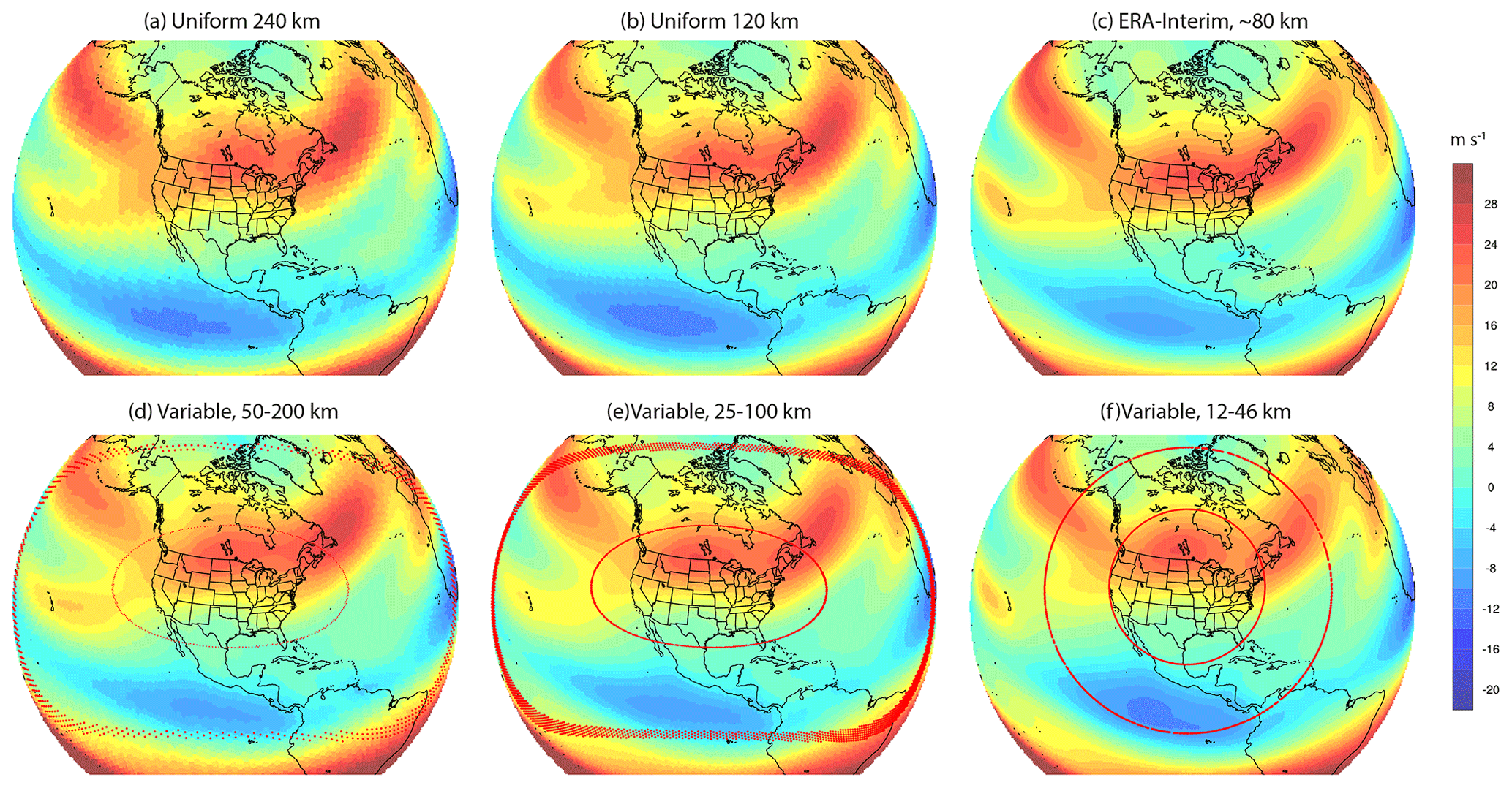
Figure 1June–July–August mean zonal wind at the 200 hPa level in each of the present-day (eval) CAM–MPAS simulations and ERA-Interim: (a) globally uniform 240 km grid, (b) uniform 120 km grid, (c) ERA-Interim, (d) variable-resolution grid with 50 km grid spacing over North America and 200 km in the coarse-resolution domain, (e) variable-resolutions from 100 to 25 km, and (f) variable-resolutions from 46 to 12 km. In panels (d), (e), and (f), grid cells at approximate boundaries between the coarse-resolution, transition, and refined domains are marked by red dots.
As a part of the structured hierarchical experiments, we have produced a regional climate dataset using a global VR dynamical core called Model for Prediction Across Scales (MPAS) coupled with the Community Atmosphere Model (CAM) physics suite. The CAM–MPAS model allows high-resolution regional simulations to be performed using regional refinement facilitated by unstructured grids, along with its non-hydrostatic dynamics, climate-oriented CAM physics parameterizations, and other Earth system component models available in the Community Earth System Model (CESM). For the dataset presented here, the model is configured on VR meshes with regional refinement over North America and quasi-uniform-resolution (UR) meshes across the globe (Figs. 1, 3). The VR configurations allow fine-scale features to be better resolved inside the refinement region; these fine-scale features then interact seamlessly with the large-scale circulations simulated at a coarser resolution outside the refined domain.
The dataset is designed to be compatible with the regional climate simulations produced for the North American Coordinated Regional Climate Downscaling Experiment (CORDEX) program (Mearns et al., 2017) (NA-CORDEX) and additional simulations using the Advanced Research Weather Research and Forecasting (WRF) model and Regional Climate Mode version 4 (RegCM4) models conducted under the HyperFACETS project. Few studies have compared limited-area and global VR dynamical downscaling approaches at the climate timescale (Hagos et al., 2013; Huang et al., 2016; Xu et al., 2018, 2021), making such comparisons an important element of the HyperFACETS project. For example, limited-area models are applied to specific regions conditioned on the global model-simulated large-scale circulation prescribed through lateral boundary conditions. Their lateral boundary conditions are identical, regardless of the resolution of the downscaling grid. In contrast, global VR models simulate both the regional and global climate in a single model. Unlike limited-area models, winds flowing into the regionally refined domain can vary with the resolutions of the coarse-resolution domains and the transition zones and potentially through the upscale effects from the high-resolution domain. As can be seen in Fig. 1, the general pattern of the large-scale winds is similar across simulations at different resolutions and in ERA-Interim (Dee et al., 2011). However, the zonal wind pattern in the eastern Pacific near California shows notable sensitivity to resolution (and bias against ERA-Interim), which could affect downwind regional hydrometeorology.
As a relatively new approach, the VR framework has not been widely used in coordinated downscaling experiments. Therefore, potential users of the CAM–MPAS climate dataset are not expected to be familiar with the characteristics of the model and the specificity regarding the model output. It is also not clear if one can apply an experimental protocol developed for regional models in a straightforward manner to global VR models. Furthermore, the timing of our production simulations coincided with the introduction of new, many-core architectures of the high-performance computing (HPC) system, such as Cori Knights Landing at the National Energy Research Scientific Computing Center (NERSC). Climate simulations of our CAM–MPAS code on such a system revealed challenges that are relevant to the wider global and regional climate simulation community. Hence, the goal of this paper is to provide a reference for not only the users of the experimental CAM–MPAS downscaled climate dataset but also the future users of the CESM2–MPAS and other global VR models for regional downscaling. Specifically, we provide a technical summary of the CAM–MPAS model (Sect. 2), details of the CAM–MPAS downscaling experiments (Sect. 3), a description of the post-processing of model output and archiving (Sect. 4), and general characteristics of model simulations (Sect. 5).
Previous works have already introduced the CAM–MPAS framework (Rauscher et al., 2013; Sakaguchi et al., 2015; Zhao et al., 2016), but, for the convenience of readers and the completeness of this document, we reiterate the descriptions of the MPAS and CAM models and their coupling in this section. More details are available from the cited references.
2.1 The Model for Prediction Across Scales (MPAS)
MPAS is a modeling framework developed to simulate geophysical fluid dynamics over a wide range of scales (Skamarock et al., 2012; Ringler et al., 2013). Currently four models based on the MPAS framework exist: atmosphere, ocean, sea ice, and land ice (The MPAS project, 2013). The atmosphere version (MPAS-Atmosphere) solves the compressible, non-hydrostatic momentum and mass-conservation equations coupled to a thermodynamic energy equation (Skamarock et al., 2012). The novel characteristic of the MPAS framework is a C-grid finite-volume scheme developed for a hexagonal, unstructured grid called Spherical Centroidal Voronoi Tessellations (SCVT; Ringler et al., 2010), accompanied by a new scalar transport scheme by Skamarock and Gassmann (2011). The SCVT mesh can be constructed to have either quasi-uniform grid cell sizes or variable ones with smooth transitions between the coarse- and fine-resolution regions (Ju et al., 2011). The C-grid staggering provides an advantage in resolving divergent flows important to mesoscale features, and the finite-volume formulation guarantees a local conservative property for prognostic variables of the dynamical core (Skamarock et al., 2012). MPAS-Atmosphere is available as a stand-alone global atmosphere model with its own suite of sub-grid parameterizations (Duda et al., 2015), but we use the MPAS-Atmosphere numerical solver as the dynamical core coupled to the CAM physics parameterizations here. Previous studies using VR meshes have demonstrated that the MPAS dynamical core is able to simulate atmospheric flow across coarse- and fine-resolution regions without unphysical signals (Park et al., 2013; Rauscher et al., 2013). This capability of regional mesh refinement is the main feature that we aim to test in the context of dynamical downscaling for regional climate projections.
2.2 The Community Earth System Model version 2 (CESM2) and Community Atmosphere Model version 5.4 (CAM5.4)
The model code base used for our simulations is a beta version of CESM2 (CESM1.5), the same code used by Gettelman et al. (2018), who focused on the regional refinement capability of the spectral element dynamical core. The atmospheric component model CAM has multiple versions of the physics parameterization package. We use the CAM version 5.4, which is an interim version toward CAM version 6 (Bogenschutz et al., 2018). The CAM5.4 physics is the default option for CAM in CESM1.5. The parameterization components in CAM5.4 are summarized in Table 1. Their characteristics are documented in detail by Bogenschutz et al. (2018), and a variety of diagnostic plots are publicly available (Atmosphere Model Working Group, 2015). A major difference between CAM5.4 and the previous version CAM5.0 is the prognostic mass and number concentrations of rain and snow in the new cloud microphysics scheme, MG2 (Gettelman and Morrison, 2015; Gettelman et al., 2015). Prognostic concentrations of precipitating particles make the model more appropriate for high-resolution simulations by removing assumptions necessary for a diagnostic approach (e.g., neglecting the advection of precipitating particles; Rhoades et al., 2018b). The prognostic aerosol scheme is also revised as the four-mode version of the Modal Aerosol Module (MAM4; Liu et al., 2016), but we only use the diagnostic aerosol scheme (Bacmeister et al., 2014) for the simulations documented in this paper. Specifically, the monthly mean aerosol mass concentrations for the year 2000 are derived from a previous simulation using CAM version 4 with the prognostic three-moment MAM (Liu et al., 2012) on a 1∘ grid. Given the prescribed aerosol mass concentrations, aerosol number concentrations are calculated by an empirical relationship between the two concentrations and are then passed to the cloud microphysics.
Bretherton and Park (2009)Park et al. (2014)Gettelman and Morrison (2015)Gettelman et al. (2015)Zhang and McFarlane (1995)Neale et al. (2008)Park and Bretherton (2009)Kiehl et al. (2000)Bacmeister et al. (2014)Iacono et al. (2008)Richter et al. (2010)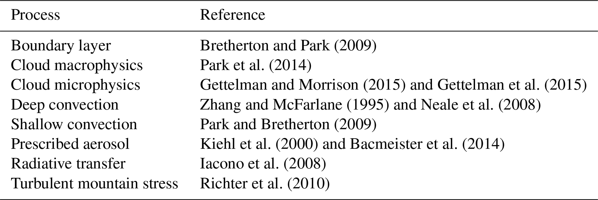
2.3 CAM–MPAS coupling
An early effort to port the MPAS dynamical core to the CESM/CAM model started in 2011 under the “Development of Frameworks for Robust Regional Climate Modeling” project (Leung et al., 2013). The hydrostatic solver of the pre-released version of MPAS (Park et al., 2013) was coupled to CAM4 by the collaborative work among Los Alamos National Laboratory, Lawrence Livermore National Laboratory, and the National Center for Atmospheric Research. This CAM–MPAS model was extensively evaluated through a hierarchy of experiments (Hagos et al., 2013; Rauscher et al., 2013; Rauscher and Ringler, 2014; Sakaguchi et al., 2015, 2016; Zhao et al., 2016). Those studies demonstrated the ability of VR simulations to reproduce the uniform, globally high-resolution simulations inside the refined domain in terms of the characteristics of atmospheric circulations as well as the sensitivity of the physics parameterizations to horizontal resolution. In the idealized aquaplanet configuration with the older CAM4 physics, the resolution sensitivity of moist physics leads to unphysical upscale effects (Hagos et al., 2013; Rauscher et al., 2013), but these artifacts are mostly muted when an interactive land model is coupled, along with the presence of other forcing such as topography and land–ocean contrast (Sakaguchi et al., 2015). The non-hydrostatic version of the MPAS dynamical core (the released version 2) was later coupled to CESM version 1.5 to understand the behavior of the CAM5 physics under a wide range of resolutions over seasonal or longer timescales (Zhao et al., 2016; Hagos et al., 2018). Hagos et al. (2018) used this model with a convection-permitting VR mesh (4–32 km) to study the sensitivity of extreme precipitation to several parameters in the CAM5 physics, demonstrating stable coupling between the non-hydrostatic MPAS dynamical core and the global model physics package CAM5 at kilometer-scale resolution. The CAM–MPAS model for the present work is similar to the one used by Hagos et al. (2018), except that MPAS v2 is replaced by a more recent version (version 4). The same CAM–MPAS version employed in this study has demonstrated robust performance in simulating the Asian monsoon system using a 30–120 km VR mesh (Liang et al., 2021).
The CAM–MPAS coupling is illustrated in Fig. 2 along with the process-coupling sequence in the host model CESM1.5. The coupling between the non-hydrostatic MPAS and the main driver of CAM uses a Fortran interface and calling sequence similar to the default finite-volume (FV) core and other dynamical cores available in CAM (Neale et al., 2010). With this coupling approach, the dynamical core can be switched from the default FV to MPAS core by simply providing a flag “CAM_DYCORE=mpas” to the CESM build script (env_build.xml), along with an appropriate name of the horizontal grid (e.g., “mp120a” has been defined for the UR120 grid following CESM Software Engineering Group, 2014). The vertical grid in CAM–MPAS follows the height-based coordinate used by MPAS-Atmosphere (Klemp, 2011), but the number of layers (32) and the height of the interface levels are configured to closely match those of the hybrid σ-p coordinate used by other CAM dynamical cores.
The CESM coupler is responsible for time step management and sequential coupling of component models (Fig. 2). When CAM is called by the coupler, the CAM driver cycles the dynamics, physics parameterizations, and communication with the coupler. When the dynamics is called by the CAM driver, the MPAS dynamical core receives tendencies of horizontal momentum, temperature, and mixing ratios that are predicted by physics parameterizations and the other CESM component models and that are summed by the CAM driver prior to the communication with MPAS. MPAS cycles its time steps from the previous atmospheric state with the physics tendencies used as forcing terms. After MPAS completes its (sub) time steps, the updated atmospheric and tracer states are passed to CAM through the interface, including hydrostatic pressure, pressure thickness of each grid box, and geopotential height. The last three variables are required by the CAM physics that operates on a vertical column under hydrostatic balance, without the need to know that the vertical column is discretized in a height-based or hybrid pressure-based coordinate. No vertical interpolation nor extrapolation is performed in coupling CAM and MPAS. The CAM–MPAS interface layer also calculates hydrostatic pressure velocity and performs other required conversions (e.g., converts the prognostic winds normal to cell edges to conventional u and v winds at cell centers and converts mixing ratios defined with dry air in MPAS to those with moist air in CAM). Note that the pressure vertical velocity ω passed from MPAS to the CAM driver is diagnosed under the hydrostatic balance and is different from the non-hydrostatic vertical velocity prognostically simulated in the MPAS dynamical core.
A second-order diffusion is added to the top three model layers to produce the so-called “sponge layers” following other CAM dynamical cores (Jablonowski and Williamson, 2011; Lauritzen et al., 2012, 2018). The top model level is located at about 45 km above sea level. This model top is higher than those typically used in MPAS-Atmosphere (≈30 km). On the other hand, the number of vertical levels in CAM5.4 is smaller than the default number of vertical levels in the MPAS-Atmosphere (41 in version 4), resulting in a relatively coarse vertical resolution for a mesoscale model. However, its vertical resolution is within the range used by regional models participating in NA-CORDEX (18–58 levels across models).
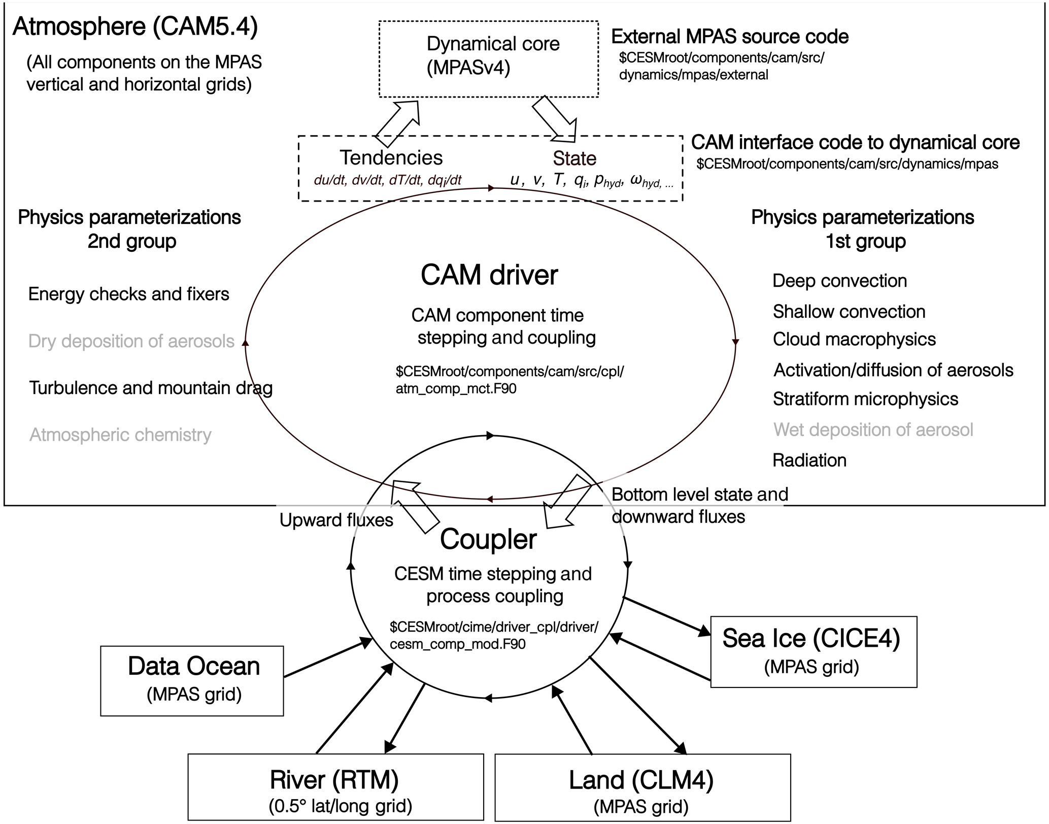
Figure 2Process coupling sequence in the CAM–MPAS model in the AMIP configuration. The MPAS dynamical core receives the time rate of change in zonal and meridional winds (u, v), atmospheric temperature (T), and water in vapor and condensed phases (qi, with , ... for water vapor, cloud liquid, cloud ice, etc.) and returns an updated atmospheric state, in terms of u, v, T, qi, hydrostatic pressure (Phyd), pressure velocity (ωhyd), etc., after integrating adiabatic dynamics. Also shown are the names of the source code files and directories where the coupling operations are carried out. The shell variable “$CESMroot” refers to the top-level directory of the CESM code. The parameterizations shown in gray were not active in our CAM–MPAS simulations.
This experimental version of CAM–MPAS is available from our private repository on GitHub (see the “Code and data availability” section), but it is not an official release and does not offer the same technical support as other CAM versions. Some model structural differences between CAM and MPAS, such as the vertical coordinate, require further work to improve physical consistency throughout the coupling processes. An ongoing effort to port MPAS to CAM/CESM addresses those remaining technical issues as part of the System for Integrated Modeling of the Atmosphere (SIMA) project (Gettelman et al., 2021; Huang et al., 2022).
3.1 Model grid and parameters
Three VR grids (50–200, 25–100, and 12–46 km) and two UR grids (240 and 120 km) are used for the CAM–MPAS downscaling experiment (Table 2). Figure 3 illustrates the UR and VR grids and the distributions of grid cell spacing in the three VR grids. The five CAM–MPAS model resolutions are named UR240, UR120, VR50-200, VR25-100, and VR12-46. UR240 has a similar grid spacing to the Max Planck Institute Earth System Model low-resolution version (MPI-ESM-LR; Giorgetta et al., 2013), whose ocean and sea-ice output is used as boundary forcing for the future experiment (see below). The UR120 grid has a comparable resolution to those of the majority of CMIP5 and CMIP6 models. Although their grid spacing does not exactly match those of the coarse-resolution domains on the VR grids nor the MPI-ESM-LR model, these two UR meshes are readily available from the MPAS website and serve as a reference for the VR simulations. The two VR grids, VR50-200 and VR25-100, are created for this project because similar VR grids were not available from the MPAS mesh archive when the project started. The two meshes are designed to have a rectangular-shaped high-resolution domain over CONUS (Fig. 3), resembling the regional model domain for NA-CORDEX (CORDEX, 2015). The 12–46 km VR mesh is obtained from the MPAS mesh archive and has a circular and slightly smaller (by ≈30 %) high-resolution domain than the other two VR grids but still covers the most of North America (Fig. 1f).
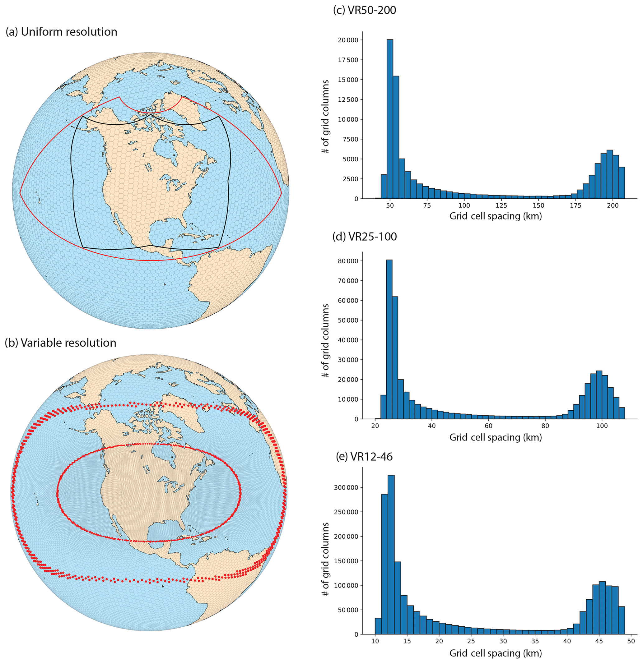
Figure 3Illustration of the MPAS meshes used for this study: (a) uniform resolution (240 km) and (b) variable resolution (50–200 km). In panel (a), the black line represents the approximate domain for the NA-CORDEX experiment and the red line represents the area covered by the NAM grids for post-processed CAM–MPAS data. In panel (b), approximate boundaries between the 50 km domain and transition zone and between the transition zone and the 200 km domain are marked by red markers. The three histograms show the numbers of grid columns binned by grid cell spacing (km) for (c) VR50-200, (d) VR25-100, and (e) VR12-46.
Table 2List of simulations. The simulation period does not include 1–2 spin-up years. Regional grids are used for post-processed data and defined in NA-CORDEX (except for NAM-88i and NAM-176i, which are defined in a similar manner to the other NA-CORDEX grids).
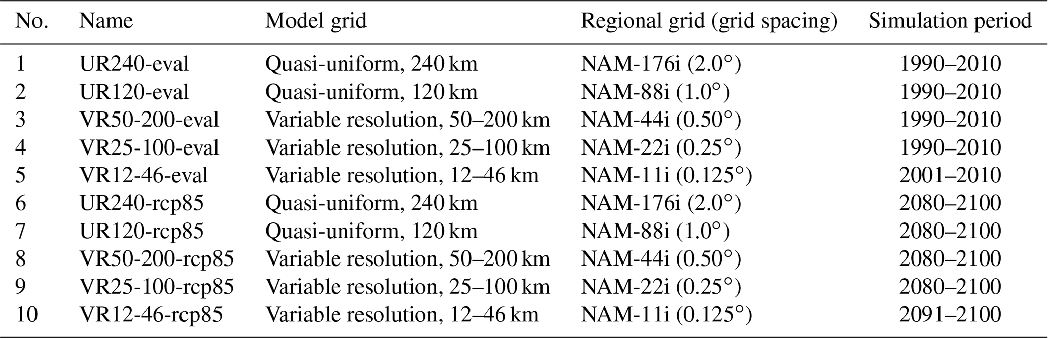
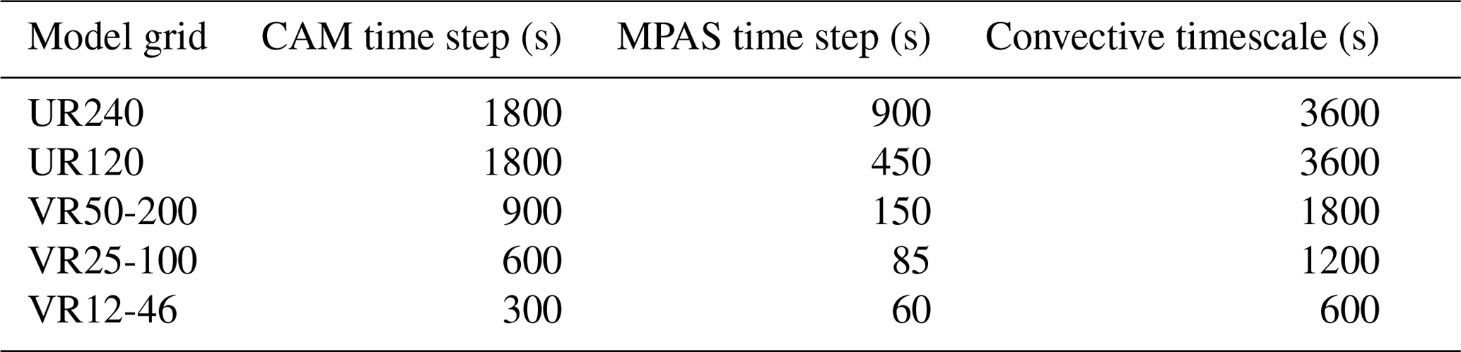
As the default parameters in the CAM5.4 physics are tuned for the prognostic MAM4 model, we retuned CAM5.4 with the prescribed aerosol and the CAM default FV dynamical core on its nominal 1∘ global grid. No attempt has been made to tune model parameters differently for the MPAS dynamical core nor at each resolution. While we are aware that resolution-dependent tuning and/or scale-aware physics schemes are necessary to fully take advantage of increased resolution (Bacmeister et al., 2014; Xie et al., 2018), tuning each resolution for both global and regional climate requires extensive effort (e.g., Hourdin et al., 2017) and is left for future work. We also note that resolution-dependent tuning is not usually done for the limited-area models that participated in NA-CORDEX and HyperFACETS nor in other coordinated projects that cover multiple model resolutions (e.g., Haarsma et al., 2016). The following parameters, however, are changed for each resolution: time step lengths, numerical diffusion coefficients, and the convective timescale used in the Zhang–McFarlane (ZM) deep-convection scheme (Table 3). In VR simulations, the dynamics time step is constrained by the smallest grid spacing in the refined region (Δx). The dynamics time steps are initially set as and further adjusted to avoid numerical instabilities that tend to occur within the stratospheric jet over the Andes. The physics time step is scaled from the default 1800 s for grid spacing using the same ratio as grid spacing changes. The convection timescale is then adjusted to scale with the physics time step in order to reduce sensitivities to horizontal resolution and time step (Mishra and Srinivasan, 2010; Williamson, 2013; Gross et al., 2018).
Table 3Resolution-dependent parameters. The default physics time step and convective timescale are 1800 and 3600 s, respectively.
3.2 Model configurations
For all of our simulations, we use a predefined CESM component set “FAMIPC5” that automatically configures CESM and its input data (e.g., trace gas concentrations) following the protocol of the Atmosphere Model Intercomparison Project (AMIP; Gates, 1992). In this configuration, the atmosphere and land models are active, whereas the sea surface temperature (SST) and sea-ice cover fraction (SIC) are prescribed. The River Transfer Model (RTM) is also active to collect terrestrial runoff into streamflow (Oleson et al., 2010), but it serves only for a diagnostic propose because the ocean model is not active. The so-called “data ocean” model reads, interpolates in time and space, and passes the input SST to the CESM coupler, which calculates fluxes between the atmosphere and ocean (CESM Software Engineering Group, 2014). The Community Ice Code version 4 (CICE4) is run as a partially prognostic model by reading prescribed sea-ice coverage and atmospheric forcing from the coupler to calculate ice–ocean and ice–atmosphere fluxes (Hunke and Lipscomb, 2010).
The land component is the Community Land Model version 4 (CLM4; Lawrence et al., 2011), which simulates vertical exchanges of energy, water, and tracers from the subsurface soil to the atmospheric surface layer. CLM4 takes a hierarchy-tiling approach to represent unresolved surface heterogeneities, distinguishing physical characteristics among different surface land covers (e.g., vegetated, wetland, lake, and urban), soil texture, and vegetation types (Oleson et al., 2010). While CLM4 is able to simulate the carbon and nitrogen cycles and transient land cover types, these biogeochemical functionalities are turned off. Instead, our simulations use a prescribed vegetation state (leaf area index, stem area index, fractional cover, and vegetation height) that roughly represents the conditions around the year 2000 based on remotely sensed products (Lawrence et al., 2011). The land cover types are also prescribed as the conditions around the year 2000 and are fixed throughout the simulations in both the eval and rcp85 experiments. These land surface settings are again consistent with the models that participated in NA-CORDEX. Note that the spatial resolution of the original data to derive CLM's land surface characteristics varies from 1 km to 1.0∘, with 0.5∘ being considered as the base resolution (Oleson et al., 2010). These input data are available from the CESM data repository (CESM Software Engineering Group, 2014).
The process coupling in CESM has already been illustrated in the previous section (Sect. 2.3, Fig. 2). In our experiment, the CLM4 land model, data ocean, and CICE4 sea-ice model are configured to run on the MPAS horizontal grid. This way, the state and flux data between different model components do not need to be horizontally interpolated during the model integration. The RTM model in a diagnostic mode runs on its own 0.5∘ grid. The data ocean and RTM communicate with the coupler once and eight times per day, respectively, while CAM, CLM4, and CICE4 run and communicate through the coupler at the same time step.
3.3 Model experiments and input data
The experiment is composed of decadal simulations for the present day and the end of the 21st century under the Representative Concentration Pathway (RCP) 8.5, featuring a business-as-usual scenario leading to a radiative forcing of 8.5 W m−2 by the end of this century. The two simulations are named following the CORDEX project protocol: “eval” denotes the historical simulations using reanalysis data for boundary conditions for its principal role of model evaluation against observations; “rcp85” denotes the future simulations in which the external forcings follow the RCP8.5 scenario and the ocean and sea-ice boundary conditions are prescribed by adding the global climate model (GCM)-simulated climate change signals to the historical observations, the so-called pseudo-global-warming experiment. We selected the MPI-ESM-LR model from the eight GCMs considered in NA-CORDEX (McGinnis and Mearns, 2021) based on its good performance with respect to the warm-season precipitation over the western and central US (Chang et al., 2015; Sakaguchi et al., 2021).
All of the input data required to reproduce our simulations are publicly available (see the “Code and data availability” section). The SST and SIC for the eval run are taken from the ERA-Interim reanalysis (Dee et al., 2011). The 6 h ERA-Interim SST and SIC data are averaged to daily values and provided to the model as input; they are then bilinearly interpolated to the MPAS grids by the CESM coupler during model integration. Other model input data include surface topography, initial conditions, and remapping weights between different input data and model grids (Appendix A). All of the surface-related input data are remapped to each MPAS grid prior to the simulations following the CESM1.2 and CLM4 user guide (CESM Software Engineering Group, 2014; Kluzek, 2010). A set of high-level scripts is now available to help prepare input data for the FAMIPC5 and other similar CESM experiments (Zarzycki, 2018). Topography input is generated by the stand-alone MPAS-Atmosphere code (init_atmosphere; Duda et al., 2015), which uses the GTOPO global 30s topography data (Gesch and Larson, 1996) as the input. The sub-grid topography information required by the gravity wave drag and turbulent mountain stress parameterizations in CAM5.4 are produced using the NCAR_Topo tool by Lauritzen et al. (2015).
As stated above, the future simulation is conducted using the pseudo-global-warming approach (e.g., Haarsma et al., 2016) based on the climate change signal simulated by the MPI-ESM-LR model from the CMIP5 archive. Specifically, annual cycles of the daily climatological SST and SIC are obtained from the historical and RCP8.5 simulations of the MPI-ESM-LR model (ensemble member id r1i1p1), and differences between the two periods are calculated for each day of the year and each grid point. This daily climatological difference (ΔSST and ΔSIC) is then added to the SST and SIC from the ERA-Interim data and is prescribed to the model. Other external forcings of solar irradiance, greenhouse gas, ozone, and other tracer gas concentrations are the same as the CESM1.2 RCP8.5 simulation conducted for CMIP5, except for the prescribed aerosol concentrations and land cover characteristics being kept the same as the eval simulation.
The annual average ΔSST and ΔSIC are shown in Fig. 4e and f, respectively. While the SST and SIC distributions in the present-day period are reasonably simulated by MPI-ESM-LR, regional biases exist over the Southern Ocean, North Atlantic, and off the west coasts of North and South America and South Africa (Fig. 4a–d). Because ΔSST and ΔSIC are added onto the climatology from ERA-Interim, the future SST and SIC forcings given to CAM–MPAS are different from those in the MPI-ESM-LR model over the biased regions. In Sect. 5.2.2 and Appendix E, we briefly compare the CAM–MPAS historical climate and its response to the external forcings with those of the MPI-ESM-LR model. It is shown that, while the base state climate differs between the two models, their changes into the future are rather similar under the same ΔSST and ΔSIC. Also of note is that the SST or near-surface air temperature (TAS) biases and their changes in the MPI-ESM-LR simulations differ from those of fully coupled CESM simulations with CAM5 or CAM6 (Meehl et al., 2012, 2013; Danabasoglu et al., 2020). Specifically, our CAM–MPAS downscaling data describe the response of the atmosphere to the ocean conditions derived from the external data (as is the case for regional model simulations in NA-CORDEX), which may be very different from the climate evolution simulated by CAM–MPAS being coupled to an active ocean model. Because CAM–MPAS and other VR atmosphere models are typically a part of global coupled climate models, it is possible to run a fully coupled VR simulation, which provide climate change signals that have co-evolved with the same atmosphere model.
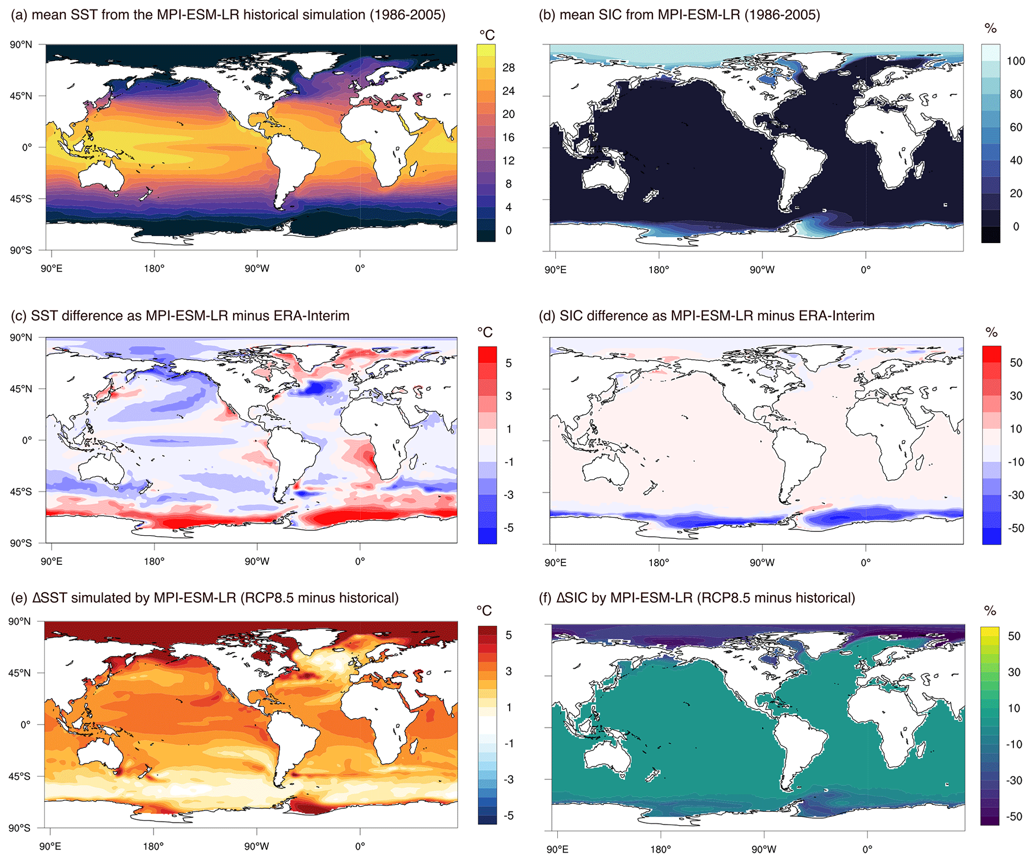
Figure 4Climatological mean sea surface temperature (SST) and the sea-ice cover fraction (SIC) from the MPI-ESM-LR model: (a) annual mean SST, (b) annual mean SIC, (c) SST bias against ERA-Interim, (d) SIC bias, (e) SST change from the historical to RCP8.5 period, and (f) SIC change over the same time periods. The historical and RCP8.5 averages are calculated over the 1986–2005 and 2080–2099 periods, respectively.
Limited-area models participating in NA-CORDEX include another historical simulation called “hist”, in which the lateral and bottom boundary conditions are provided by the driving global models. Also the rcp85 simulations in NA-CORDEX use GCM output directly for boundary conditions (“direct downscaling”), in contrast to adding the climate change signals to the observed present-day boundary conditions. We do not conduct the hist experiment with CAM–MPAS, as our principal goal is to assess the credibility of dynamically downscaled climate by the CAM–MPAS atmosphere model in comparison to observational and other downscaled data, which, at a minimum, requires (1) the eval run with the prescribed ocean boundary conditions from observations, isolating the CAM–MPAS model's bias without the influence of the GCM's SST and sea-ice biases, and (2) the model response to external forcings associated with global warming, which can be reasonably assessed by the pseudo-global-warming experiment (see the general agreement in the large-scale climate response between the CAM–MPAS and MPI-ESM-LR models in Sect. 5.2.2). An advantage of the global VR simulation in pseudo-global-warming approach is that, unlike adding the mean atmospheric climate change signals to the lateral boundary conditions for regional models, a global VR simulation does include variability and high-order atmospheric responses to the warming. Because our dataset does not have the hist experiment, we will use the terms “eval”, “historical”, and “present-day” interchangeably to refer to the eval simulations.
The atmospheric initial condition for the eval experiment is taken from the ERA-Interim data on 1 January 1989 at 00:00 UTC for all simulations except for the VR12-46 simulation that used data from 1 January 2000 at 00:00 UTC. The land initial condition is taken from the output valid for 1 January 2000 at 00:00 UTC from a 0.5∘ fully coupled CCSM4 simulation for the historical period (CESM, 2016). The CLM4 land state on the 0.5∘ grid is remapped to the MPAS grids following Kluzek (2010). Starting from these initial conditions, the model is run for 1 year to spin up the eval simulations. For the future rcp8.5 experiments, the initial condition for each resolution is taken from the 1 January 2011 state of the corresponding eval simulation, followed by 2 years of spin-up simulations. We found that these spin-up lengths are sufficient for the CONUS domain, but they are not necessarily adequate in the deep soil layer for the global domain, particularly at high latitudes (as will be discussed in Sect. 5.2).
4.1 Post-processing
To facilitate comparison with other regional models in the NA-CORDEX model archive, the model output on MPAS's unstructured mesh is remapped to a standard latitude–longitude regional grid defined by the NA-CORDEX project (the so-called NAM grid; Fig. 3 and Table 2). Variable names and units used in CAM/CESM are converted to those of NetCDF Climate and Forecast (CF) Metadata Conventions (version 1.6) that are used by NA-CORDEX. Three-dimensional atmospheric variables defined on the terrain-following model coordinate are vertically interpolated to the NA-CORDEX-requested pressure levels (200, 500, and 850 hPa). The following describes how such post-processing was performed.
We mainly used the Earth System Modeling Framework (ESMF) library (Balaji et al., 2018) through the NCAR Command Language (NCL) (UCAR/NCAR/CISL/TDD, 2017a) for regridding MPAS output. The ESMF library provides several remapping methods, among which the first-order conserve method is used for extensive variables and fluxes, and the patch recovery method is used for all other variables. For variables required at a specified pressure level, we first linearly interpolate from the model height level to the pressure level, followed by horizontal remapping. The order of the vertical vs. horizontal interpolation is not expected to be important for the accuracy of subsequent analyses (Trenberth, 1995). Note that the three pressure levels available in the post-processed archive are not sufficient to close budget equations of vertically integrated quantities such as moisture and energy (Bryce Harrop, unpublished result). For moisture budget analyses, data users are encouraged to use the vertically integrated moisture fluxes and water vapor path available in the daily variables (Appendix C2). For other variables, it is possible to retrieve them at more pressure levels from the monthly or 6-hourly raw model output (Appendix B).
Missing values exist in some variables in the raw model output on the MPAS grids, e.g., soil moisture in the grid points where 100 % of the grid point area is covered by ocean, lake, or glacier. The locations of such missing values do not change with time, and the corresponding grid points are masked when generating regridding weights. Time-varying missing values arise during vertical interpolation to a pressure level over the areas where surface topography crosses the target pressure level. We followed the guidance provided by the NCL website to regrid such time-varying missing values (UCAR/NCAR/CISL/TDD, 2017b). Specifically, we first remap a binary field defined on the source MPAS grid: all values are one where the vertically interpolated pressure-level variable is missing, and they are zero everywhere else. By remapping such a field from the original MPAS grid to the destination grid, we can identify, using nonzero values, which destination grid points are affected by the missing values on the original grid, and the remapped pressure-level variables in these destination grid boxes are set missing. This rather cumbersome procedure can be replaced by a remapping utility recently enhanced in the NetCDF Operator (NCO; Zender, 2017).
Table 4Mean (mm d−1), variance (mm2 d−2), kurtosis, and selected percentiles (mm d−1) of daily precipitation sampled from the central-eastern United States (30–47∘ N, 85–105∘ W) on the original and remapped grids with grid spacings similar to the original grid. “XXX to YYY” in the row header refers to results on the remapped grid, e.g., “VR25-100 to NAM-22i” means that the statistics are calculated on the NAM-22i grid to which precipitation fields are remapped from the original MPAS grid. The seventh and last rows show the results after remapping twice, whereby precipitation fields are remapped from the VR25-100 (or WRF 25 km) grid to the NAM-22i grid and then remapped back to the original VR25-100 (or WRF 25 km) grid. The first-order conserve remapping method is used for all of the results. The analysis domain covered in the WRF output on the curvilinear grid is slightly smaller than the domain used for MPAS, hence the disagreement in statistics between these two model groups. The statistics are based on the years 2001–2005, except for the fifth and sixth rows where data from the 1991–1995 and 1996–2000 periods are used, respectively.
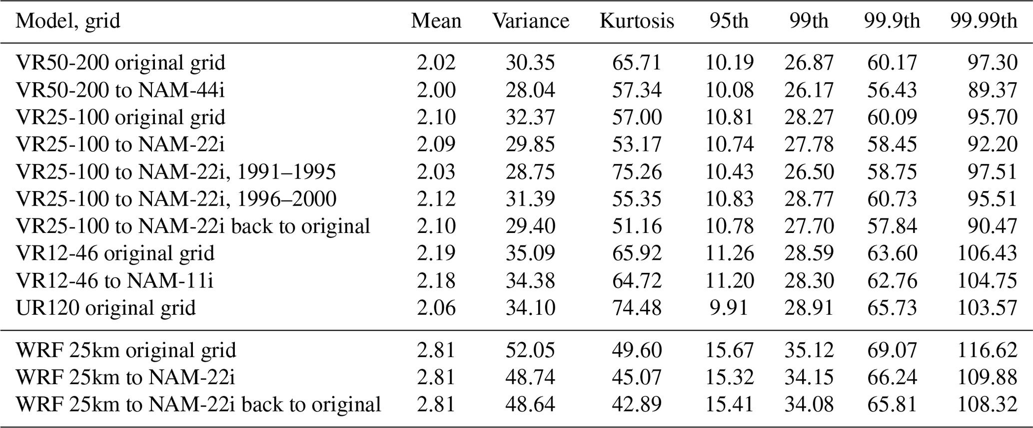
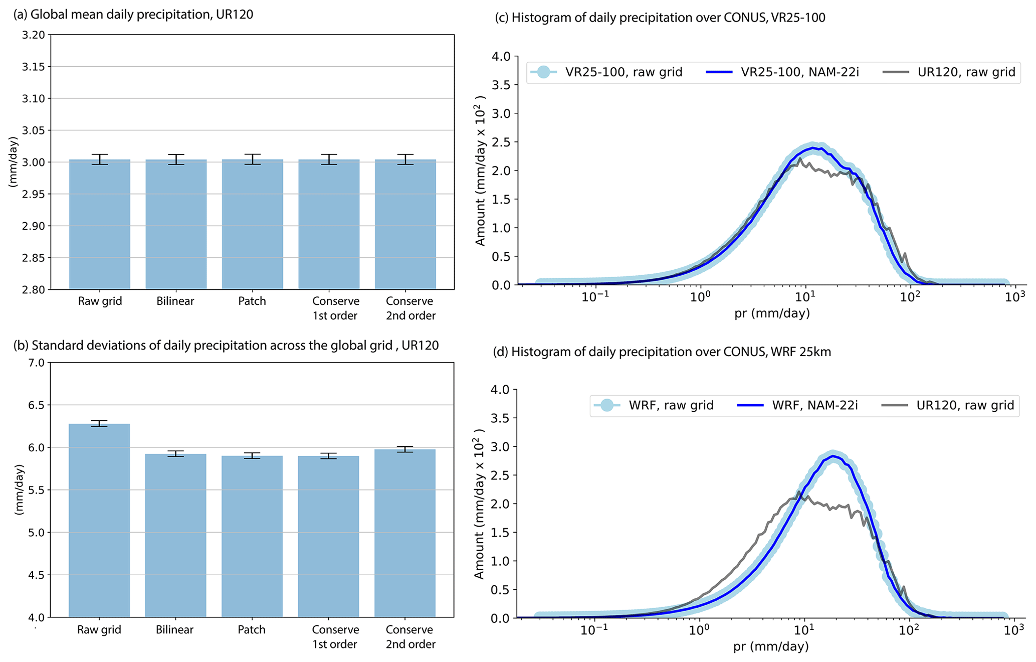
Figure 5Comparison of regridded daily precipitation using four different methods: (a) global annual average of precipitation in UR120 and (b) standard deviations of precipitation across the global grid in UR120; (c) daily rain rate amount distributions over CONUS calculated on the original MPAS grid in VR25-100 (dark blue line), on the remapped (first-order conserve) latitude–longitude NAM22 grid in VR25-100 (light blue circles), and on the original MPAS grid in UR120 (gray line); and (d) daily rain rate amount distributions over CONUS calculated on the original WRF grid in the NA-CORDEX WRF 25km simulation (dark blue), on the remapped NAM22 grid in the WRF 25km simulation, and the UR120 histogram, as in panel (c), for comparison. The statistics are based on a 10-year period from 1990 to 1999, and the error bars in panels (a) and (b) show the 95 % confidence interval based on the year-to-year variance. The distributions of rain rate amount are calculated following Pendergrass and Hartmann (2014), using the minimum rain rate of 0.029 mm d−1 and a 7 % spacing.
NA-CORDEX documents minor artifacts due to interpolation by the patch recovery method (e.g., small negative values for nonnegative variables such as relative humidity) (Mearns et al., 2017). The influence of horizontal regridding, or interpolation, on the statistics has also been noted by previous studies (Chen and Knutson, 2008; Diaconescu et al., 2015). To understand the effect of regridding in our post-processing, Fig. 5 compares selected statistics calculated on the original and remapped daily precipitation using different remapping methods, bilinear, patch recovery, first-order conserve, and second-order conserve, available from the ESMF library (Balaji et al., 2018). The regridding effect on the (spatial) mean is negligibly small using any of the regridding methods. As shown in Fig. 5a, the global annual mean precipitation (3.004 mm d−1) is nearly identical (to the accuracy of 10−3 mm d−1) for the original and the regular 1∘ latitude–longitude grid after remapping.
The variance loss due to remapping is typically ≈6 %–8 % for daily precipitation. The magnitude of variance loss depends on which variable is remapped – a variable with a smoother spatial structure than precipitation (e.g., atmospheric temperature) is less affected by regridding. At the global scale, ≈6 %–8 % loss of variance can be larger than year-to-year sampling variability, as illustrated in Fig. 5b. The second-order conservation method retains the spatial variance slightly better than the other methods. At regional scales, sampling uncertainty from different time periods (each sample is 5 years long here) can be as large as the smoothing effect. This is illustrated in Table 4 (from the third to sixth rows) based on the statistics of daily precipitation in the CONUS sub-domain east of the Rockies, calculated on the original VR25-100 grid and conservatively remapped to the NAM-22i grid. We avoid the Rockies and other mountainous regions where year-to-year variability is so large that our sample size is not long enough to reliably estimate spatial variances. The third and fourth rows present the statistics on these two grids from the years 2001 to 2005, while the fifth and sixth rows are from the years 1991 to 1995 and 1996 to 2000, respectively, on the NAM-22i grid. The 5-year average of the spatial variance is 32.37 mm d−1 on the original grid for 2001–2005, which is reduced to 29.85 mm d−1 after regridding. The spatial variance from the other 5-year period can differ from the variance from 2001 to 2005 by as much as the regridding loss. Similar magnitudes of smoothing effect and sampling uncertainty are also found in kurtosis and extreme values represented by the 95th to 99.99th percentiles. These differences are not visible on the daily precipitation histograms calculated on the original VR25-100 grid, the remapped NAM-22i grid, and the UR120 output on its raw MPAS grid for the same CONUS sub-domain (Fig. 5c). The two histograms of VR25-100 are visually identical, and the difference from the UR120 precipitation is clearly distinguishable.
Two other points notable in Table 4 are as follows: (1) the smoothing effect becomes weaker with finer grid resolutions based on the three VR resolutions and (2) successive remapping back from the regional NAM-22i to the original grid (the seventh row) leads to a further loss of the variance and other moments but to a lesser degree compared with the first remapping. Similar smoothing effects from the first and second remapping are observed in the output from the WRF model on a 25 km grid from the NA-CORDEX archive. Despite the fact that WRF uses a regular latitude–longitude grid that is similar to the NAM-22i grid, regridding effects on the selected statistics resemble those on the CAM–MPAS output. For example, regridding VR25-100 output loses ≈8 % of the daily precipitation variance by the first remapping, while the 25 km WRF simulation loses 6 %. The histograms of daily precipitation in the WRF 25 km simulation are shown in Fig. 5d, again confirming that the histograms are not visually affected by regridding. Given such a priori knowledge of the regridding effect and sampling uncertainty at regional scales, we do not expect that the remapping effect would seriously affect the statistical inference of regional climate metrics.
4.2 Data repositories
Post-processed monthly and daily variables in the “essential” and “high priority” list of the NA-CORDEX archive (Mearns et al., 2017) are accessible from the Pacific Northwest National Laboratory DataHub. All of the variables and temporal frequencies are available from the NERSC High Performance Storage System (HPSS), made accessible through web browsers by the NERSC Science Gateway Service (see the “Code and data availability” section). All variables requested from the experiment protocol are two-dimensional at a single level. Appendix C lists the post-processed variables.
File names, attributes, and coordinates of the reported variables and their file specification follow the CORDEX archive design (Christensen et al., 2014) and NA-CORDEX data description (Mearns et al., 2017). The file name is composed of the following elements: [variable name].[scenario].[driver].[model name].[frequency].[grid].[bias correction].[start month]-[end month].[version].nc. In the CAM–MPAS dataset, the scenario is either eval for the historical period or rcp85 for the pseudo-warming future simulation. The driver is “ERA-Int” for the historical period and “ERA-Int-MPI-ESM-LR” for the rcp85 case. Post-processing of the current CAM–MPAS simulations does not involve any bias corrections; hence, it is labeled as “raw”. The major version refers to different production simulations, and the minor version refers to changes/corrections in the post-processing stage. The publicly available CAM–MPAS output is either “v3” or “v3.1”; the major version is 3 because it was necessary to rerun simulations twice due to major changes in model configurations, and the minor revision involves a different treatment of missing values arising from vertical interpolation to a pressure level (see Sect. 4.1). With the other straightforward file name elements, an example file name for a daily precipitation data in the historical run of CAM–MPAS VR50-200 reads as follows: pr.eval.ERA-Int.cam54-mpas4.day.NAM-44i.raw.198901-201012.v3.nc. In contrast, an example file name for a daily precipitation data in the future pseudo-warming reads as follows: pr.rcp85.ERA-Int-MPI-ESM-LR.cam54-mpas4.day.NAM-44i.raw.207901-210012.v3.nc.
Raw CAM–MPAS output on the global MPAS grid (i.e., not remapped to a regional latitude–longitude grid) is also available from the NERSC HPSS space. Appendix B provides more information about the MPAS unstructured mesh, links to the archive directory, and other resources to help analyze the raw MPAS data. The NERSC data archive also contains example scripts and variables necessary to process model variables on the MPAS grid (e.g., latitude and longitude arrays).
5.1 Computational aspects
In this section, we discuss some computational aspects of our simulations, as one of the motivations to use a global VR framework is its computational advantage compared with a global high-resolution simulation. On the other hand, global VR simulations are expected to be more expensive than limited-area model simulations if the cost for the host GCM simulations that provide boundary conditions is not considered. For example, the VR grids used in this study have 1.1–2.6 times more grid columns than the limited-area grids used by the RegCM4 and WRF models in the NA-CORDEX and HyperFACETS archives (Tables 5, F2). Here, we do not compare the simulation cost of the CAM–MPAS VR configurations against regional models but instead focus on how the cost of CAM–MPAS simulations differs between the UR and VR grids and between the lower and higher resolutions.
All of our simulations were run at NERSC. The following result is obtained from the production simulations and not a systematic scaling analysis of the CAM–MPAS code nor NERSC systems. The system configurations (e.g., number of nodes) of our production simulations are not only based on good throughput but also on simulation cost as well as expected queue wait time (Fig. D1), which often accounts for the majority of the total production time (e.g., the average queue wait time for VR25-100 is approximately 3 times the actual computing time). All simulations used only the distributed-memory Message Passing Interface (MPI) parallelism, i.e., shared-memory parallelism (OpenMP) is not used. The main computing system at NERSC switched from Edison to Cori when the production simulations of the CAM–MPAS model were starting (NERSC, 2021). The newer system Cori is partitioned into two subsystems, Cori Haswell (HW) and Cori Knights Landing (KNL). As discussed below, the CESM–CAM–MPAS code showed large differences in performance on KNL and other systems, posing a significant impact on our production cost. Interested readers are referred to Appendix D for further details of our runtime configurations and the characteristics of the NERSC systems.
Three simulations that are not part of the CAM–MPAS downscaling dataset are also included in the following as references: (1) the default FV dynamical core on the nominal 1∘ grid (FV 1∘), (2) the same model configuration as UR120 but using the newer version of the CAM–MPAS model that will be released as an official option of CESM2 (UR120-new), and (3) CAM–MPAS on a quasi-uniform 30 km grid (UR30). These three simulations were run for other projects but with a similar set of file output (monthly, daily, 6 h, 3 h, and hourly output) for more than 5 years. All simulations use the same CAM5.4 physics with prescribed aerosol.
Table 5Simulation throughput and cost. The simulation cost is based on so-called “NERSC hour” (which is calculated as the number of nodes × number of hours × machine-dependent charge factor × queue priority factor), assuming the “regular” queue, and shown in units of 103 NERSC hours per simulated year (NERSC ). Throughput () is an average of at least 60 jobs, with the standard deviation shown in parentheses. Ncalc is the number of time steps per day over all grid boxes . Most of the samples are production runs, except for UR120-new, FV 1∘, and UR30, which are not the part of the dataset described in this paper but are shown as references.
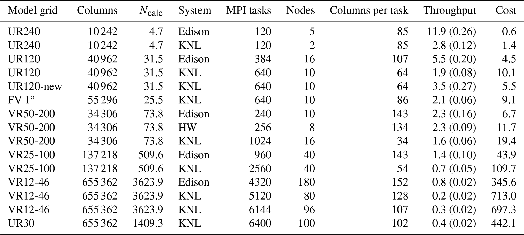
Figure 6a visualizes the simulation cost vs. total MPI tasks used, as often used in cost-scaling studies. Table 5 lists the numerical values used in the figure. Although scatters in the data from different computing systems are notable, there is a clear trend to which we can fit a curve. The blue line represents a power function (y=axb) fitted to the simulation cost in the log–log space. The exponent b (the slope of a straight line on the log–log plot) is 1.54 with a 95 % confidence interval of 0.50, exhibiting a weak but nonlinear increase. The nonlinear increase is expected because linearly increasing cost is only possible for an idealized case, as also shown in the figure. The green line represents an ideal situation that the parallel part of the code speeds up linearly with additional resources (an ideal weak scaling; Eq. 5.14 in Hager and Wellein, 2011), whose cost thus increases linearly with the number of MPI ranks (slope of 1). The orange line of a constant cost applies only to the case where the size of the problem (e.g., number of grid columns) stays the same so that using more resources shortens the simulation time. This is an ideal “strong scaling” and is not applicable to the cost scaling for different resolutions over a fixed global domain. It is obvious from this comparison that larger resource use for higher resolutions on a fixed domain size, such as the global domain, always increases the computing cost nonlinearly.
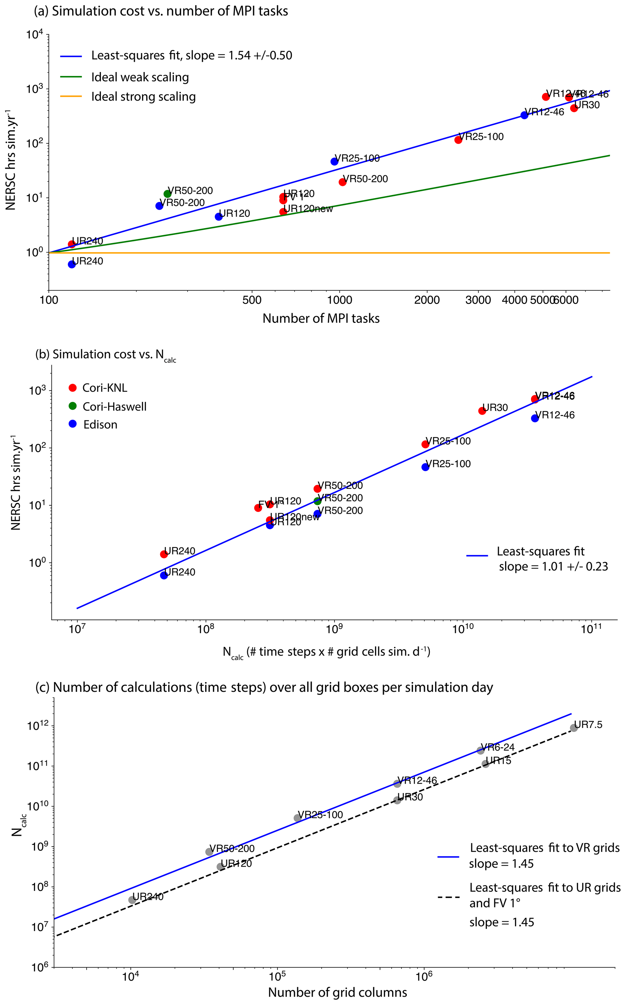
Figure 6Graphs showing the relationship between (a) the simulation cost in terms of NERSC hours per simulated year (NERSC h sim. yr−1) and number of MPI tasks, (b) simulation cost and Ncalc (number of calculations equals the physics and dynamics time steps per simulated day across the global domain), and (c) Ncalc and the number of grid columns. The parameters of the fitted linear lines (blue curves, linear in the log–log space), , are shown in the legend. UR120-new refers to the UR120 simulation using the new CAM–MPAS code under development. In panel (c), we added data points for a variable-resolution 6–24 km mesh (VR6-24) as well as uniform resolution with 15 and 7.5 km grid cells (UR15 and UR7.5) by using their numbers of grid columns and scaling the model time step as described in Sect. 3.
There are several reasons for the nonlinear increase in the simulation cost against resources used, such as communication and load imbalance (Hager and Wellein, 2011; Heinzeller et al., 2016). For estimating the simulation cost of a given MPAS grid, we found that it is simpler to use the number of calculations (physics and dynamics time steps) per simulated day across all of the grid boxes in the global domain: Ncalc= (number of grid columns) × (number of vertical levels) × (number of time steps per day). Plotting simulation cost as a function of Ncalc (Fig. 6b), the fitted curve exhibits a slope of approximately 1. Looking at Ncalc as a function of the number of grid columns, it appears to be separated into two groups of VRs and URs, indicating the time step constraint from the high-resolution domains in VRs (Fig. 6c). The least-squares-fitted power functions have exponents of 1.45 for both VR meshes and UR meshes. This weak nonlinearity presumably comes from the dependence of time step length on grid spacing, which then becomes an additional implicit dependence on the numbers of grid columns.
As a specific example of VR vs. UR comparison, we take VR25-100, UR30, and UR120, as the latter two URs have comparable grid spacings in the high- and low-resolution regions of the VR25-100 grid. We use Ncalc of the simulations conducted on KNL to gauge the computational advantage of the VR25-100 against UR30, a uniform high-resolution simulation, as well as the extra cost added by the regional refinement to a uniform low-resolution simulation, UR120. The actual values of Ncalc for these three resolutions are shown in the third column of Table 5 and suggest UR30 to be 48 times more expensive than UR120 and VR25-100 to be 16 times more costly than UR120. The actual simulation cost closely follows the Ncalc scaling; 1 simulation year of UR30 (480.0×10³ NERSC h sim. yr−1) is 48 times more expensive than that of UR120 (10.1×10³ NERSC h sim yr−1.) The actual cost of VR25-100 is just 11 times that of UR120, which is lower than that expected from Ncalc, possibly reflecting the error from using an empirical curve fitted to three different systems in the single KNL system. In this case, VR25-100 achieves a factor of 4 computational advantage compared with UR30 for obtaining a similarly high-resolution grid over CONUS.
A couple of other points are noted in Table 5 and Fig. 6. First, the computational cost of CAM–MPAS UR120 and the default dynamical core FV 1∘ is comparable (1.9 vs. 2.1 sim. yr d−1 for CAM–MPAS UR120 and CAM–FV 1∘, respectively). Second, the model throughput (cost) of VR12-46 is 0.2 sim. yr d−1, half (double) that of UR30, despite the fact that these two grids have the same number of columns and that the simulations are run with similar numbers of columns per MPI task. The main reason for the difference is likely the shorter time steps (about one-third) in VR12-46 than in UR30 due to the numerical constraint imposed by the smallest grid spacing in the high-resolution domain. Lastly, we get consistently lower throughput and higher cost on Cori KNL than on the other two systems. Our experiment and previous studies (Barnes et al., 2017; Dennis et al., 2019) suggest a few compounding reasons (Appendix D), such as inefficient memory management for some global arrays, poor vectorization, and less focus on shared-memory parallelism of the CAM5/MPASv4 source code, which are not aligned well with the wider-vector and many-core architecture of KNL. However, the shorter expected queue time on KNL than HW (Fig. D1) makes KNL our main system for production. The weaker performance of the experimental CAM–MPAS code on KNL leads to a higher computational cost than our initial estimate for VR12-46, limiting the length of VR12-46 simulations to be half of other simulations. More importantly, the code characteristics described above are not necessarily unique to the CAM5/MPASv4 codes but may be common in other global or regional climate models in which many lines of the codes are written by domain scientists with little attention to code optimizations. Such climate models are not likely to be efficient on emerging, more energy-efficient HPC architecture similar to KNL for having wider vector units and more cores per node (and less memory per core) than previous systems. For example, two new systems being deployed to HPC centers in the United States – Perlmutter to NERSC (NERSC, 2022) and Derecho to the NCAR-Wyoming Supercomputing Center (NCAR Research Computing, 2022) – share such characteristics in their CPU nodes.
Fortunately, some of the computational problems with the CAM–MPAS model have been resolved through the MPAS-Atmosphere optimization, ongoing effort to port the later version 6 of MPAS-Atmosphere to CESM2 (the SIMA project), and other numerous changes across the CESM source code from CESM1.5 to CESM2. Those updates lead to an almost 80 % speedup of the UR120 throughput, as can be seen from the UR120 and UR120-new simulations in Table 5. Some of the speedup comes from different compiler optimizations used for the two simulations, but the code development plays a major role in this performance improvement. The Cori system is retiring, but the computational advantage of the new code is expected to be applicable to other systems, including the new NERSC system Perlmutter. We expect that decadal simulations on the VR12-46 grid or even convection-permitting VR meshes will be feasible using the newer CAM–MPAS code or the SIMA atmospheric general circulation model with MPAS as its dynamical core option. Multi-season convection-permitting simulations have been already carried out with the new SIMA-MPAS model (Huang et al., 2022).
5.2 General characteristics of simulated climate
We briefly review selected aspects of the simulated climate. The focus here is the climate statistics at the global-scale and over the regions outside the VR high-resolution domain of North America. This is because, although the post-processed datasets cover a broad area encompassing the NA-CORDEX domain (Fig. 3a), the limited-area grid does not allow one to infer remote sources of large-scale forcings and their dependency on model resolution, which may be important to understand processes responsible for projected changes within the high-resolution domain. Appendix E presents additional figures and a table. For the downscaled regional climate, Appendix F provides a general overview of the model performance focusing on the CONUS region. The main finding of the regional assessment is that the performance metrics of precipitation improve with higher resolution, but the results are more mixed for other variables. Moreover, the resolution sensitivity of precipitation becomes weaker within the North American domain compared with the global statistics, which is shown below. A separate, systematic investigation of the regional climate in comparison with other limited-area models is being conducted (Sakaguchi et al., 2021) and will be reported elsewhere.
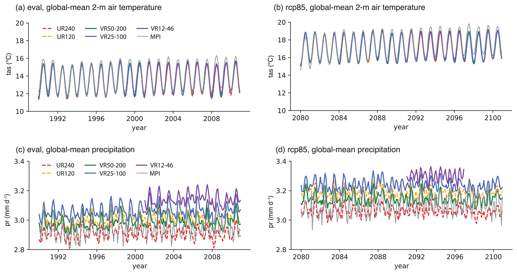
Figure 7Time series of the monthly global mean (a) near-surface air temperature (TAS) in the present-day (eval) simulations, (b) TAS in the future (rcp85) simulations, (c) precipitation (PR) in the present-day (eval) simulations, and (d) PR in the future (rcp85) simulations. “MPI” in the legend refers to the MPI-ESM-LR model simulation. The shorter VR12-46 simulation appears only in the last 11 years.
5.2.1 Present-day climate
The time evolution of global mean TAS is nearly identical across the resolutions (Fig. 7a), indicating a strong constraint by the prescribed SST. In contrast, global mean precipitation exhibits systematic differences among the resolutions such that it monotonically increases with finer resolution; UR240 simulates the lowest global mean precipitation, followed by VR50-200, UR120, VR25-100, and VR12-46 (Table 6, Fig. 7c), indicating that the coarse-resolution domain dictates the resolution sensitivity at the global scale in the VR simulations. In Fig. 7c, we see that the global precipitation of MPI-ESM-LR is similar to those of UR240 and VR50-200, which are the two resolutions closest to the MPI-ESM-LR model resolution.
Table 6 indicates that this monotonic increase is mainly contributed by convective precipitation, rather than large-scale precipitation. The trend of increasing convective precipitation with higher resolution is the inverse of what previous studies have found about the lineages of CAM physics (Williamson, 2008; Rauscher et al., 2013; Wehner et al., 2014; Herrington and Reed, 2020). This unexpected resolution sensitivity is not necessarily an improvement for the model hydrological cycle, and it is attributed to the changes that we made in the convective timescale of the ZM convection scheme (Sect. 2.2) based on our previous study (Gross et al., 2018). It would be more preferable that the total precipitation and fractions of convective (associated with unresolved updraft) and large-scale (associated with resolved upward motion) components remain unchanged for grid resolutions coarser than the so-called “gray zone” (e.g., Fowler et al., 2016). However, our result does illustrate a potential (and cursory) use of the convective timescale for tuning CAM–MPAS VR simulations. For example, smaller changes than we made in the timescale (Table 3) may result in more preferable partitioning of precipitation components. Readers are referred to Sect. 8b of Gross et al. (2018) for in-depth discussion about tuning mass-flux-based convection parameterizations for VR models. Other notable resolution sensitivities are reductions in the cloud fraction and vertically integrated cloud liquid and ice mass concentrations, which then bring about resolution sensitivities to cloud radiative forcing and radiative fluxes. Reduction in the cloud amount with higher resolutions has been noted by previous studies (Pope and Stratton, 2002; Williamson, 2008; Rauscher et al., 2013; Herrington and Reed, 2020). For example, Pope and Stratton (2002) found a 12 g m−2 reduction in the global mean cloud liquid-water path when refining the grid spacing from ≈280 to 90 km in the HadAM3 model. Herrington and Reed (2020) attributed the reduced cloud amount to stronger subsidence outside convective regions, which is linked to more intense resolved upward motion within the convective regions at higher resolution. We speculate that the same processes operate in our simulations with additional complexities due to our tuning of the ZM convection scheme.
Table 6Global and annual means of selected variables from present-day (eval) simulations, taken from the Atmospheric Model Working Group (AMWG) diagnostic package (Atmospheric Model Working Group, 2014). Abbreviations in variable names are as follows: top-of-atmosphere (TOA), shortwave radiative flux (SW), longwave radiative flux (LW), shortwave cloud radiative forcing (SWCF), and longwave cloud radiative forcing (LWCF). Observational and reanalysis data (Obs) are provided through the AMWG diagnostic package and listed in Table E1. Averages are shown for variables for which multiple observational data are available.
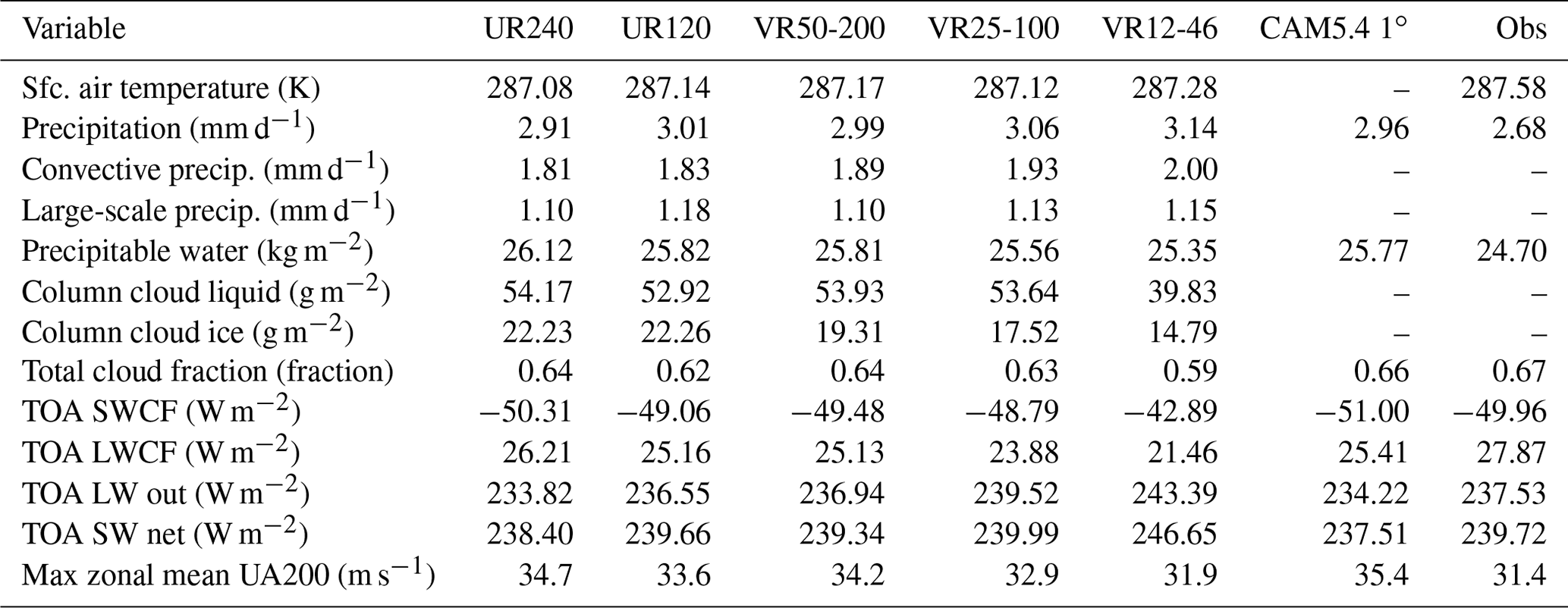
Figure 8 examines the spatial patterns of TAS and precipitation biases of VR25-100. We show VR25-100 as an example because the bias patterns are generally similar at the other resolutions (Figs. E1, E2). As with CAM5.4 and other climate models (Morcrette et al., 2018), the simulated TAS is too warm over the midlatitude continents, including the central United States (Fig. 8a). Little difference from ERA-Interim is seen over the ocean, but notable exceptions exist over the Southern Hemisphere storm track (≈0.5 ∘C) and the Arctic ( ∘C). The TAS bias appears similar to that of CAM5.4 with the default 1∘ FV dynamical core (Atmosphere Model Working Group, 2015), indicating a more important role of physics parameterizations than resolution or dynamical core for the bias (Appendix E).
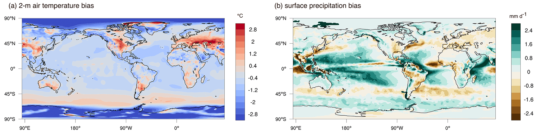
Figure 8Difference in the climatological mean (a) 2 m air temperature over the 1990–2010 period between CAM–MPAS VR25-100 and ERA-Interim as well as (b) surface precipitation over the 1997–2010 period between VR25-100 and the Global Precipitation Climatology Project (GPCP). The ERA-Interim sea surface temperature and sea-ice cover are used as input for the CAM–MPAS AMIP simulations. The CAM–MPAS output and the reference data (ERA-Interim and GPCP) are remapped from their original grids to a global latitude–longitude grid with a ≈0.7∘ grid spacing, which is a similar resolution to the ERA-Interim grid.
The resolution sensitivity of the global mean precipitation (Table 6c) originates mostly from the tropics between 20∘ S and 20∘ N (Figs. 8b, 9a) where the model overestimates precipitation compared with the Global Precipitation Climatology Project (GPCP). This regional bias generally becomes worse with higher resolution. While the tropics is far away from the downscale target of North America, tropical precipitation bias may have remote effects on large-scale circulations over the midlatitudes through Rossby waves and subtropical jets (Lee and Kim, 2003; Christenson et al., 2017; Dong et al., 2018; Wang et al., 2021). Such remote effects seem small over North America but much more prominent in the Southern Hemisphere, consistent with the previous VR CAM–MPAS study (Sakaguchi et al., 2015). For example, steady changes across resolution appear in the zonal mean sea level pressure in the tropics and in the high latitudes, with clearly greater magnitude in the Southern Hemisphere than in the Northern Hemisphere (Fig. 9b). Consistently, zonal mean zonal wind also shows stronger resolution sensitivities over the tropics and Southern Hemisphere than in the Northern Hemisphere (Fig. E3). The Atmosphere Model Working Group (2015) shows a similar sea level pressure bias in the default CAM5.4, and the apparently large magnitude of the bias depends on which reanalysis dataset is used as a reference. Notably, higher resolution reduces the biases of sea level pressure and zonal mean zonal wind over the Southern Hemisphere.
In our global pseudo-warming experiment, differences between the CAM–MPAS and MPI-ESM-LR simulations in large-scale circulations are also important to understand the processes underlying regional climate change over North America. Figure 10 compares the climatological mean zonal wind at the 200 hPa level (UA200) and zonal anomalies of 500 hPa geopotential height (ZG500) from the VR25-100 and MPI-ESM-LR simulations of the historical period. We continue to use VR25-100 as an example because differences between the two models (MPI-ESM-LR and CAM–MPAS) are substantially larger than the resolution sensitivities of the CAM–MPAS model (not shown). With respect to VR25-100, Fig. 10a, b, and c indicate that (1) the midlatitude (eddy-driven) jet is located at higher latitudes, (2) the subtropical jet over North America is stronger, and (3) the Walker circulations over the Pacific and Atlantic oceans are also stronger than those in the MPI-ESM-LR model. Notable differences in ZG500 include a stronger ridge in VR25-100 than in the MPI-ESM-LR model over the western North America (Fig. 10d, e, f). The stronger ridge and associated static stability, along with different jet locations and strengths, indicate that the two models simulate the generation and propagation of atmospheric disturbances differently as well as the local response to them, which are all factors that are suggested to be important for the hydroclimate of the western and central US (e.g., Leung and Qian, 2009; Song et al., 2021).
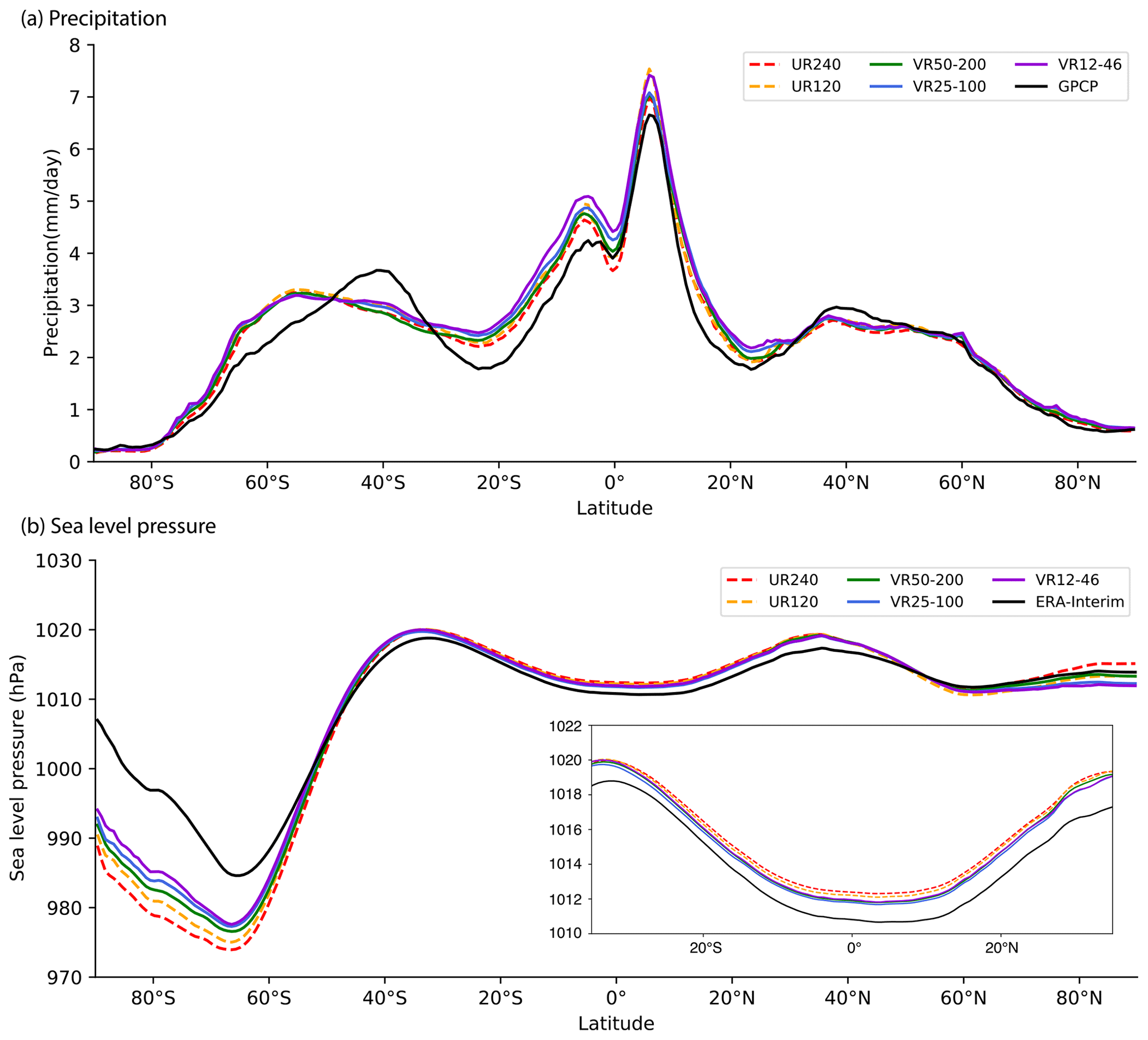
Figure 9Zonal and annual mean (a) precipitation and (b) sea level pressure from the CAM–MPAS simulations and reference data of (a) GPCP and (b) ERA-Interim. All data are first remapped to a ≈0.7∘ latitude–longitude grid before taking the zonal average. The inset in panel (b) shows the same mean sea level pressure but only in the region between 35∘ S and 35∘ N.
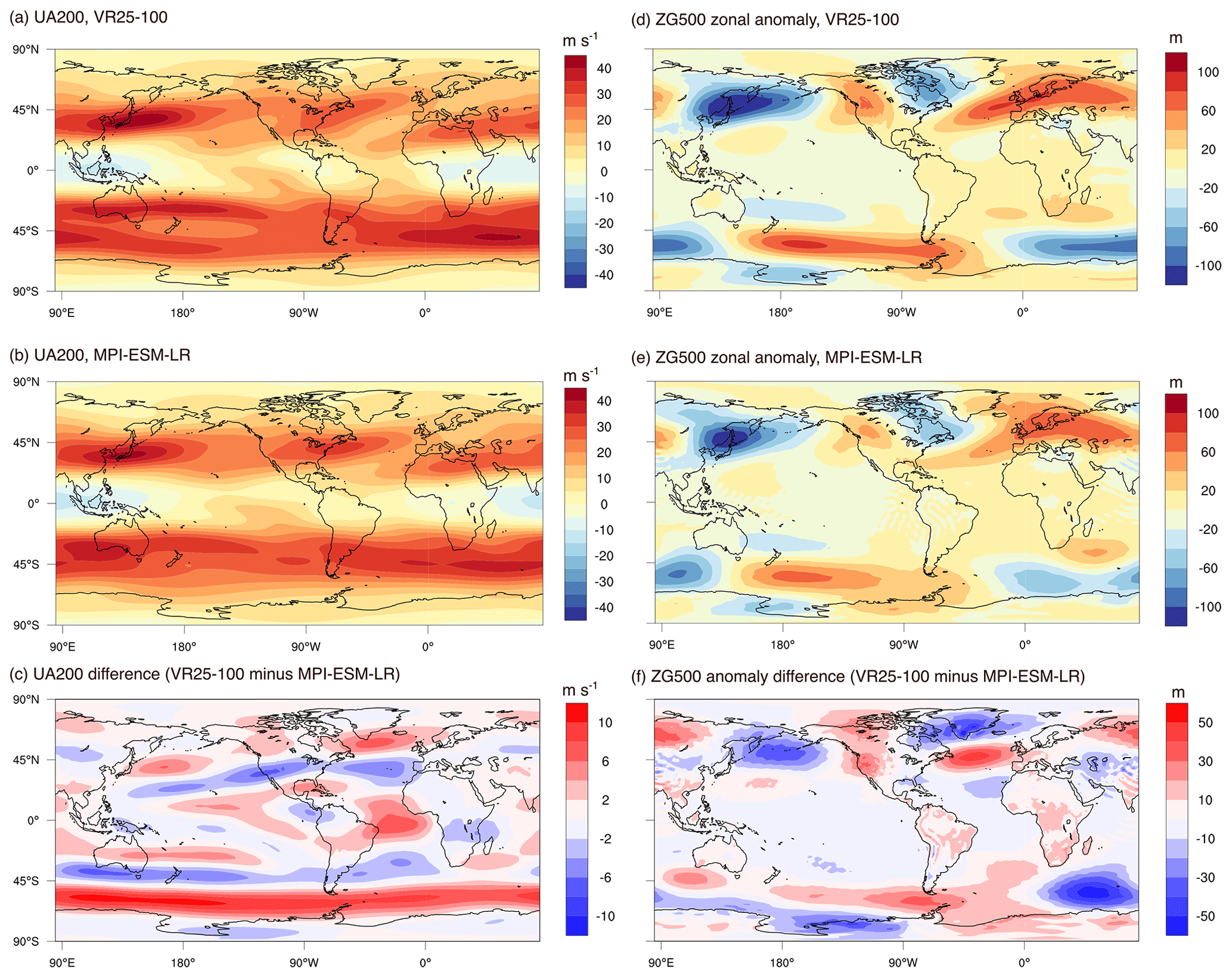
Figure 10Annual mean zonal wind at the 200 hPa level in (a) VR25-100 and (b) MPI-ESM-LR as well as (c) the difference between the two simulations. Geopotential height at the 500 hPa level in (d) VR25-100 and (e) MPI-ESM-LR as well as (f) the difference between the two simulations. All data are remapped to a latitude–longitude grid by the patch method (Balaji et al., 2018). The wavy patterns in panels (e) and (f) near the Andes are likely numerical oscillations in the MPI-ESM-LR model (Geil and Zeng, 2015).
5.2.2 Future climate
The global mean TAS remains insensitive to resolution in the future rcp85 case (Fig. 7b). Also similar to the historical period, we see steady increase in global mean precipitation with finer resolution (Fig. 7d). As a result, all of the resolutions project similar changes in the global mean precipitation (ΔP) from the historical to the rcp85 case within the range of 0.15–0.18 mm d−1.
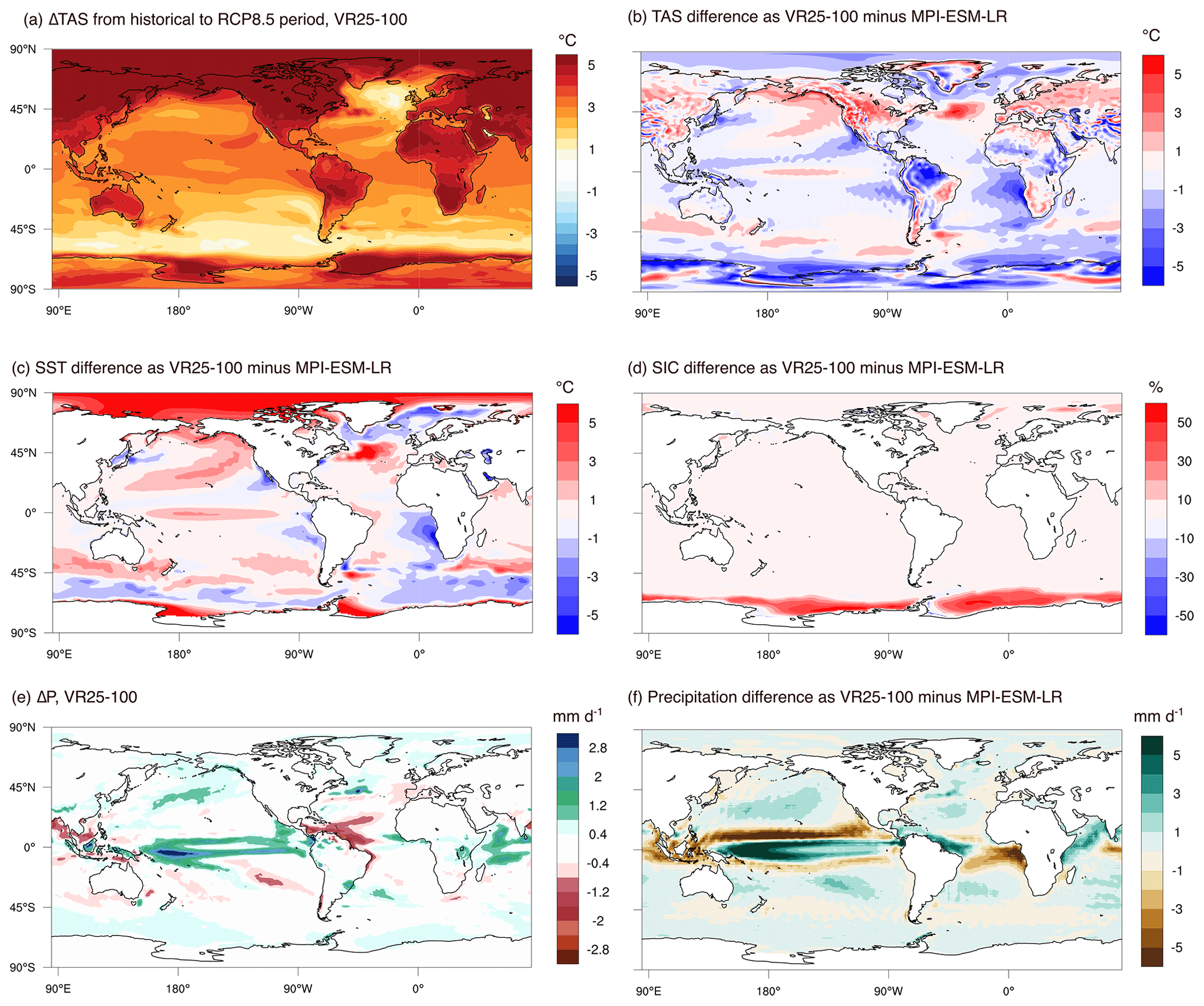
Figure 11Spatial patterns of the near-surface climate change from the historical (1990–2010) to the future RCP8.5 case (2080–2100) and the difference in the mean future climate between the VR25-100 and MPI-ESM-LR simulations: (a) simulated change in the near-surface air temperature (ΔTAS) in VR25-100, (b) difference in the mean TAS between VR25-100 and MPI-ESM-LR in the RCP8.5 simulations, (e) precipitation change (ΔP) in VR25-100, and (f) precipitation difference between the two RCP8.5 simulations. Panel (c) is the same as panel (b) but for SST difference, and panel (d) is the same as panel (b) but for SIC difference.
Looking at the spatial patterns, the TAS change (ΔTAS) from the historical to the RCP8.5 period in VR25-100 closely follows the ΔSST patterns derived from the MPI-ESM-LR model (by comparing Figs. 4e and 11a). The almost identical ΔSST leads to a different climatological SST (and TAS) in the two future simulations (Fig. 11b) because ΔSST and ΔSIC from MPI-ESM-LR are added to the base state from ERA-Interim instead of the MPI-ESM-LR model itself (Fig. 11c, d). It is notable that the SST over the Arctic region is substantially warmer in VR25-100 than in MPI-ESM-LR, while such a difference is lacking in TAS (Fig. 11b, c). The discrepancy is the result of an assumption in the CESM data ocean model such that SST below −1.8 ∘C (a typical freezing temperature of sea ice) is reset to this assumed freezing temperature, and the SST shown in the figure is not the input to the model but output from the simulation. In the MPI-ESM-LR simulation without such an assumption, the climatological SST can be as low as −5 ∘C over the Arctic region. We presume that this SST difference does not directly affect TAS because of the Arctic sea-ice cover.
The spatial pattern of ΔP in VR25-100 is characterized by a marked increase in the tropical Pacific, Arabian Sea, and Northern Hemisphere storm tracks and by a reduction over the tropical Atlantic Ocean (Fig. 11e). These ΔP responses over the ocean generally agree with the MPI-ESM-LR projection (Fig. E4), while the extent of regional features differ, especially in the equatorial region, such that precipitation from the Intertropical Convergence Zone (ITCZ) is projected to be more intense in a narrower band in VR25-100 than in MPI-ESM-LR. Over land, ΔP in the two simulations diverges most notably in the Amazon Basin as well as in Australia, southern Africa, and, importantly, North America. These changes over land become more visible in the ocean-masked contour plots in Fig. E5e and f. Those regions are also where we see the resolution sensitivity of ΔP among the CAM–MPAS simulations (Fig. E5b, c, d, e, f), indicating a large uncertainty in the projection of regional hydrological cycles.
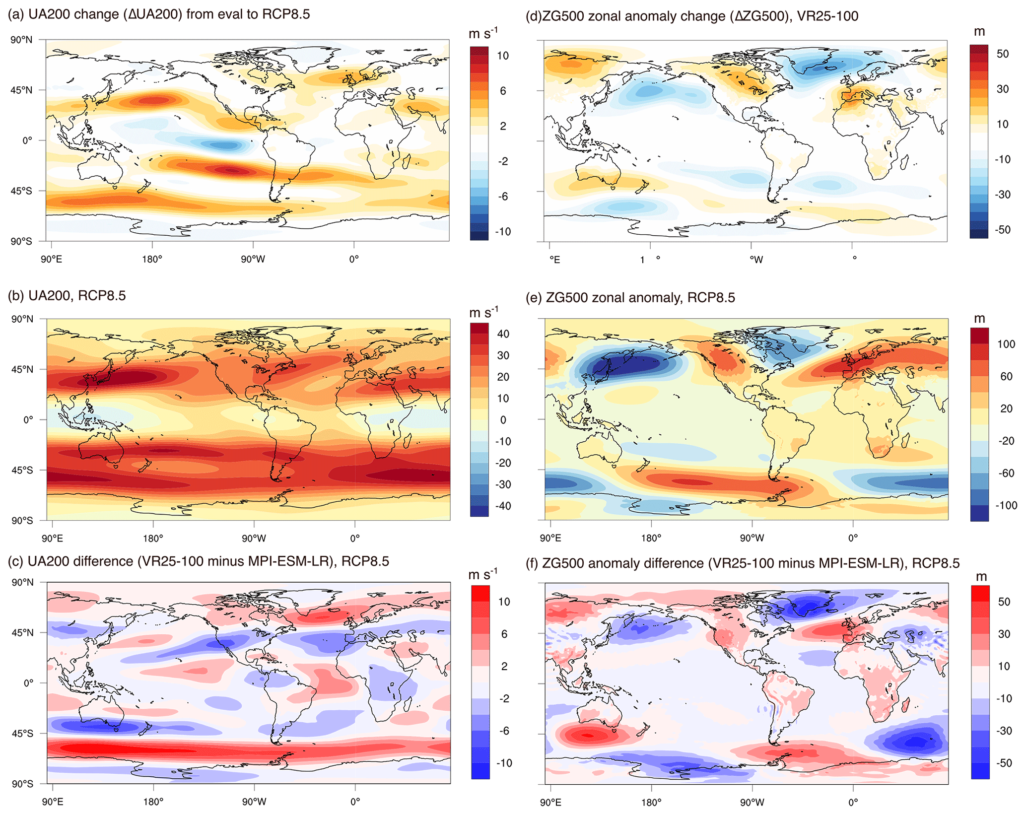
Figure 12Simulated changes in the annual mean upper-level circulations from the historical (1990–2010) to the future RCP8.5 case (2080–2100) and the difference in the future climate between the VR25-100 and MPI-ESM-LR simulations: (a) the 200 hPa zonal wind change (ΔUA200) in VR25-100, (b) the future UA200 climatology in VR25-100, (c) the UA200 climatology difference between VR25-100 and MPI-ESM-LR in the RCP8.5 period, (d) the simulated change in zonal anomaly 500 hPa geopotential height (ΔZG500) in VR25-100, (e) the future climatology of ZG500 zonal anomaly in VR25-100, and (f) the ZG500 difference between VR25-100 and MPI-ESM-LR.
Turning to the large-scale circulations, the projected change in the 200 hPa level zonal winds (ΔUA200) in VR25-100 indicate broader and more intense subtropical jets, midlatitude storm tracks, and Southern Hemisphere polar jet at the end of the 21st century (Fig. 12a, b). MPI-ESM-LR also projects such changes in terms of the zonal mean circulation (Shaw, 2019), and the spatial patterns of ΔUA200 are generally consistent between the two models with a pattern correlation of 0.87 (Fig. E6). The projected changes in the zonal anomaly of the 500 hPa geopotential height (ΔZG500) in VR25-100 are characterized by the pattern shift to the east over middle to high latitudes in the Northern Hemisphere (Fig. 12d, e). The shift is simulated by MPI-ESM-LR and also found in the CMIP5 multi-model mean response (Wills et al., 2019). Because the responses of these large-scale circulations to the imposed radiative forcings and (identical) ocean warming are similar in the two models, the base state differences, as seen in Fig. 10c and f, remain nearly unchanged in the future period (Fig. 12c, f). Therefore, distinct aspects of the large-scale forcings on the North American climate, as discussed in the previous section, will continue to be seen in the RCP8.5 case.
5.2.3 Soil spin-up
Lastly, we would like the readers to be aware of soil spin-up at deep layers in the cold regions outside the refined region. A previous study (Cosgrove et al., 2003) and community experience from the NA-CORDEX program (Mearns et al., 2017) suggest that 1 year is enough for the model soil state to reach a quasi-equilibrium over the CONUS region (i.e., excluding permafrost regions from North America), provided that a reasonably realistic soil moisture distribution is used for the spin-up initial condition (i.e., not an idealized state such as spatially uniform soil moisture content). This is the case for the soil liquid water in the present-day (eval) simulations with a 1-year spin-up starting from a condition taken from a previous CCSM4 historical simulation (Sect. 3). Using VR50-200 as an example, the CONUS-averaged soil liquid water does not show a systematic drift at any soil model levels, and neither does the global average (Fig. 13a, b, d). The CONUS-averaged soil ice does not show an obvious trend either (Fig. 13c). However, the global-average soil ice in the 10th soil layer shows a clear increasing trend in the first ≈10 years (Fig. 13e). Such a drift appears in the layer around 1 m deep and becomes stronger with depth (not shown). Because the same land model CLM4 is used in this study and in the CCSM4 historical simulation, this adjustment is likely a response to different land model resolutions and different atmospheric states. Similarly, the global mean soil ice in the rcp85 experiment shows a steep decline in the first ≈10 years (after the 2-year spin-up), followed by a still decreasing but weaker trend afterwards (Fig. 13f). It is not clear that the weaker trend after 10 years represents the response to the future transient forcing or if it is still converging to the model's own equilibrium state.
Spatially, most of the soil ice is stored over the Northern Hemisphere high latitudes and the Tibetan Plateau; therefore, the spin-up drift only exists in the limited regions that are in the coarse-resolution domain in our VR grids (Fig. 14). Previous land modeling studies on permafrost regions suggest timescales of 100 years for the water and energy cycles (Elshamy et al., 2020; Ji et al., 2022), especially with the extended bedrock layers down to ≈50 m deep in CLM4 (Lawrence et al., 2008, 2012). We note that the global mean temperature of the bottom bedrock layer keeps increasing throughout the rcp85 experiment, with an overall increase of ≈3 K over the 20-year period (not shown).
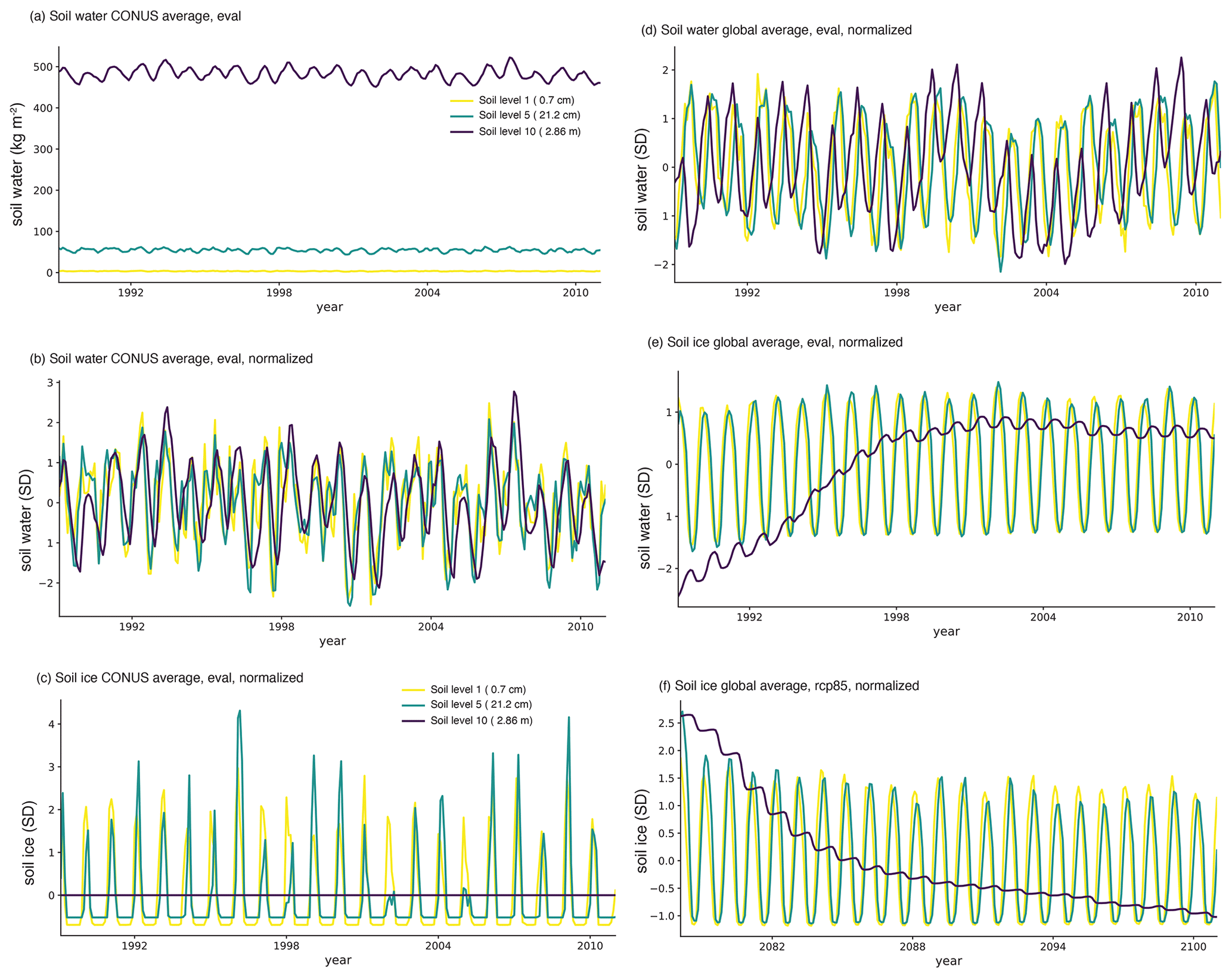
Figure 13Time series of monthly mean (a) soil liquid water in the 1st, 5th, and 10th model layers averaged over the CONUS region in the VR50-200 eval experiment; (b) soil liquid water in the 1st, 5th, and 10th model layers averaged over the CONUS region in the VR50-200 eval experiment but normalized by subtracting the temporal mean and dividing by the standard deviations; (c) normalized soil ice content averaged over CONUS; (d) globally averaged and normalized soil liquid content; (e) globally averaged and normalized soil ice content; and (f) globally averaged and normalized soil ice content from the rcp85 experiment.
These results and previous findings suggest that high-latitude and high-altitude (e.g., Tibetan Plateau) soil hydrology and thermodynamics in the deep layers require decades to centuries of spin-up. It is not clear whether the model adjustment in such a deep, remote soil state can affect the simulated climate within the target refinement region. If such a remote effect exists, then it is necessary for global VR models to spin up the high-latitude/high-altitude soil state for a downscaling experiment, although it may be relevant to regional models in NA-CORDEX for the northern part of the domain. More detailed investigations are required on the coupling between the deep soil over the high latitudes and the target downscaling region resulting from global teleconnection (e.g., by affecting the meridional temperature gradient).
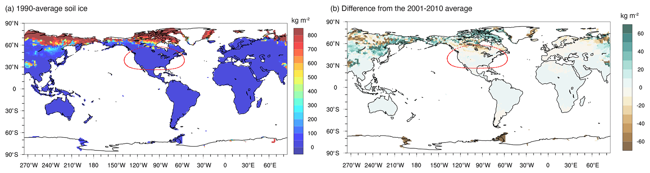
Figure 14The soil ice content summed across soil layers in the VR50-200 eval simulation as (a) an annual average over 1990 and (b) the difference between the 1990 average (immediately after the spin-up) and the last 10-year average.
The HyperFACETS project includes a large multi-institutional team and an important stakeholder engagement component to support climate adaptation efforts across a wide range of sectors. The engagement suggested that timely and comprehensive documentation of a climate model and the model output dataset is important to meet the growing demand for well-documented and well-curated regional climate datasets from climate scientists, impact assessment researchers, stakeholders, and regional and national climate assessment activities. The aim of this work is to provide such documentation for a relatively new global VR model framework and to facilitate improvement in not only the model sciences but also the technical aspects of the climate model code, experimental protocol, and workflow from model configuration to post-processing under the changing HPC environment.
The CAM–MPAS simulations described in this paper are uniquely designed to facilitate the use and evaluation of the global VR model to complement the multi-model dynamical downscaling products from the NA-CORDEX program and additional limited-area model simulations carried out under the HyperFACETS project. Details of the experimental CAM–MPAS model, downscaling simulations, output post-processing, data archive, and ongoing improvement of the CAM–MPAS model are presented. A list of available variables and resources to analyze the raw model output on the unstructured grids are provided in the Appendix section of this paper.
Model biases are described at the global (Sect. 5.2.1) and regional scale within the high-resolution domain of the VR simulations (Appendix F). It is noted that the biases are largely inherited from the CAM5.4 physics parameterizations, while some model sensitivities to resolutions and/or time step lengths are different from those reported in previous studies using the CAM physics. Precipitation changes with resolution are likely due to the resolution-dependent tuning of the convection timescale in the ZM deep-convection scheme, highlighting a potential benefit and the need for more systematic efforts of model tuning in VR downscaling. We also expect that the model biases mentioned above will be reduced in the future CAM–MPAS (SIMA-MPAS) downscaling simulations coupled to the CAM6 physics parameterizations. A different deep-convection parameterization, the Grell–Freitas scheme (Grell and Freitas, 2014), is being ported to SIMA-MPAS to alleviate several weaknesses in the CAM–MPAS VR configuration (Jang et al., 2022).
Looking ahead, an important next step would be to officially incorporate VR models into coordinated downscaling programs such as CORDEX (e.g., Prein et al., 2022). Participation of VR models allows a direct and more comprehensive intercomparison of limited-area and global VR models. As our analyses of soil state and large-scale circulations suggest, some adaptations of the experimental protocol and analysis scope are required to address differences between the two modeling frameworks. Having both limited-area and VR models in a coordinated project may also facilitate interactions between global and regional climate modeling communities, which could accelerate model development and workflow improvement to further reduce uncertainties in the regional climate dataset.
Figure A1 visualizes the input data flow for the CAM–MPAS model, as explained in Sect. 3.2. Most of the data preparation is to remap from the original input grids to the target MPAS grid, which is required for each different MPAS mesh.
Fortran namelist files that describe non-default model parameters, input data paths, output variables, and other model configurations (examples for VR25-100) are shared in a public space (https://portal.nersc.gov/cfs/m2645/pnnl/CAMMPAS/namelists, last access: 17 May 2023). A shell script (prod05_facets25-100_edison.sh) that executes a series of CESM scripts to set up CAM–MPAS VR25-100 is also available from the same directory.
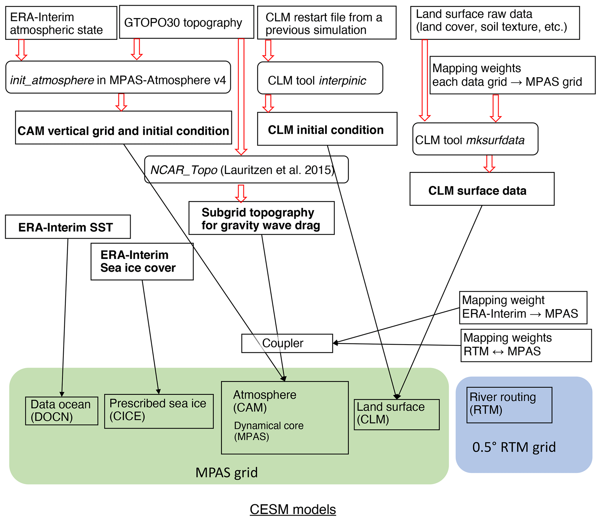
For users who prefer to analyze raw model output on the MPAS unstructured mesh, the raw output is available from https://portal.nersc.gov/archive/home/k/ksa/www/FACETS/CAM-MPAS (last access: 17 May 2023). Ancillary netCDF files for each MPAS grid are also available (https://portal.nersc.gov/cfs/m2645/pnnl/CAMMPAS/statfiles/, last access: 17 May 2023), including latitude/longitude coordinates of the grid cell centers, land–ocean masks, surface topography, and grid description in the SCRIP format (necessary to create remapping weights).
For users convenience, we provide a simple shell script to remap CAM–MPAS output to a regular latitude–longitude grid (regrid_CAM_MPAS_NCO.sh) as well as a Jupyter notebook to calculate regional statistics on the raw MPAS grid data (RegionalAverage_mpasmesh.ipynb) in another directory (https://portal.nersc.gov/cfs/m2645/pnnl/CAMMPAS/examples/, last access: 17 May 2023). In the subdirectory “postprocess_6hr/”, users can find a more involved example with an NCL script to post-process 6-hourly model output into the CORDEX format as well as shell scripts to run the NCL script in parallel on a NERSC KNL compute node using GNU Parallel (Tange, 2018).
The MPAS mesh structure and other descriptions of the MPAS-Atmosphere model are provided in the MPAS user guide (Duda et al., 2019) and at https://www2.mmm.ucar.edu/projects/mpas/tutorial/Boulder2019/index.html (last access: 17 May 2023). A number of example Python and NCL scripts to visualize data on the MPAS's unstructured grids are provided at http://mpas-dev.github.io/atmosphere/visualization.html (last access: 17 May 2023). To apply them to CAM–MPAS output, two adjustments are needed. First, variable names are different between MPAS-Atmosphere and CAM–MPAS, and the latter variable names can be found on the CAM documentation web page (e.g., https://www2.cesm.ucar.edu/models/cesm2/atmosphere/docs/ug6/hist_flds_f2000.html, last access: 17 May 2023). Second, the dimension name “nCells” is used for variables defined at cell centers in MPAS-Atmosphere, whereas the dimension name is “ncol” in CAM–MPAS.
A raw CAM–MPAS output, or history file, contains multiple variables at one or more time records (up to 24), as opposed to a post-processed file that contains a single variable over a long period of time, from 1 year to the whole simulation period. All variables in the CAM–MPAS history files are either defined at or interpolated from cell edges to cell centers. Readers are referred to the https://portal.nersc.gov/cfs/m2645/pnnl/CAMMPAS/README_history.md (last access: 17 May 2023) readme file for details of the history file format, organization, variables, etc.
List of variables available on the NA-CORDEX regional grid.
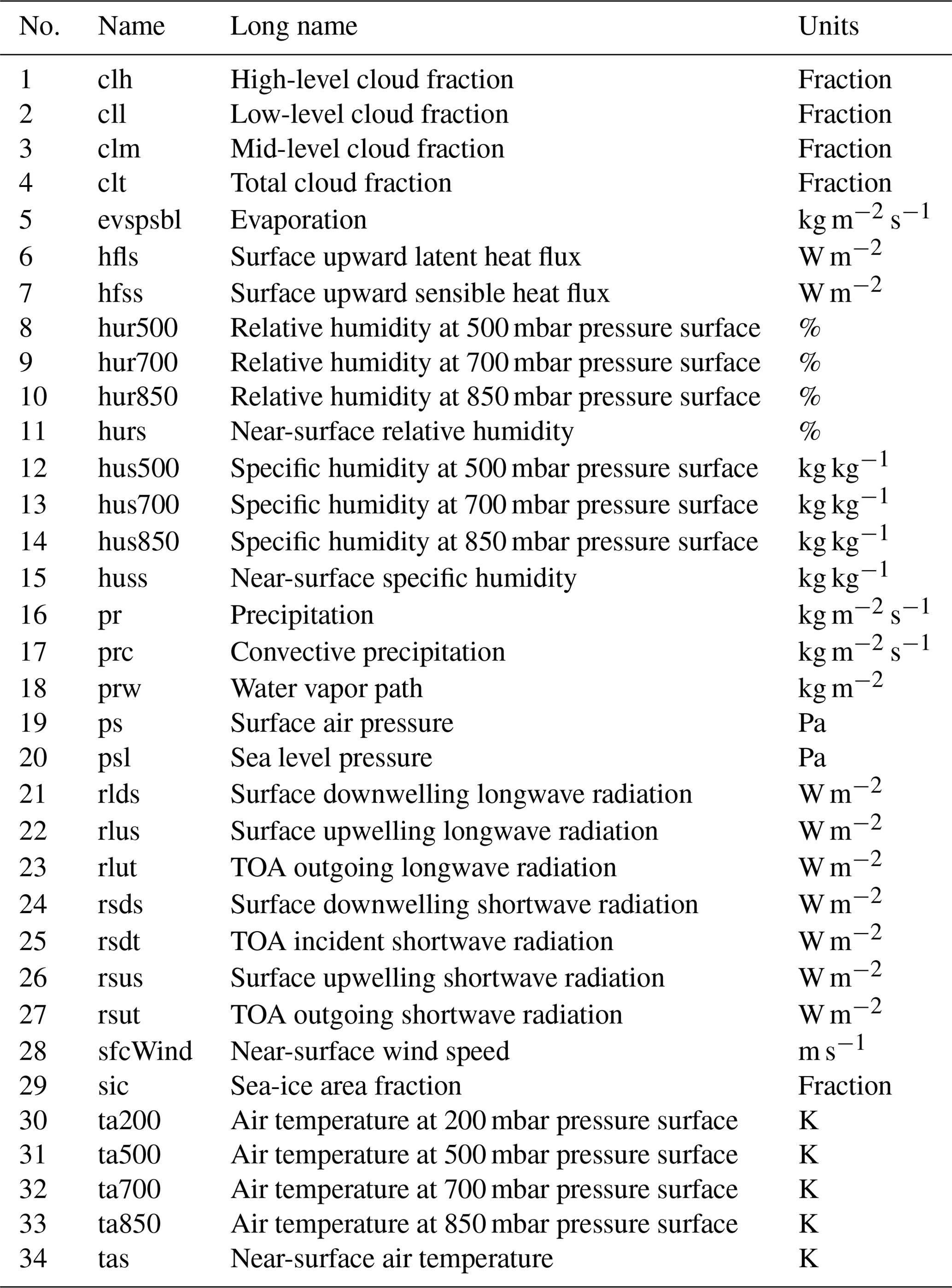
Table C2Daily variables. The lowest model level (for uas and vas) is located about 60 m above the surface. The variables in bold font are considered essential and high priority in NA-CORDEX and are available from both the PNNL DataHub and NERSC Science Gateway.
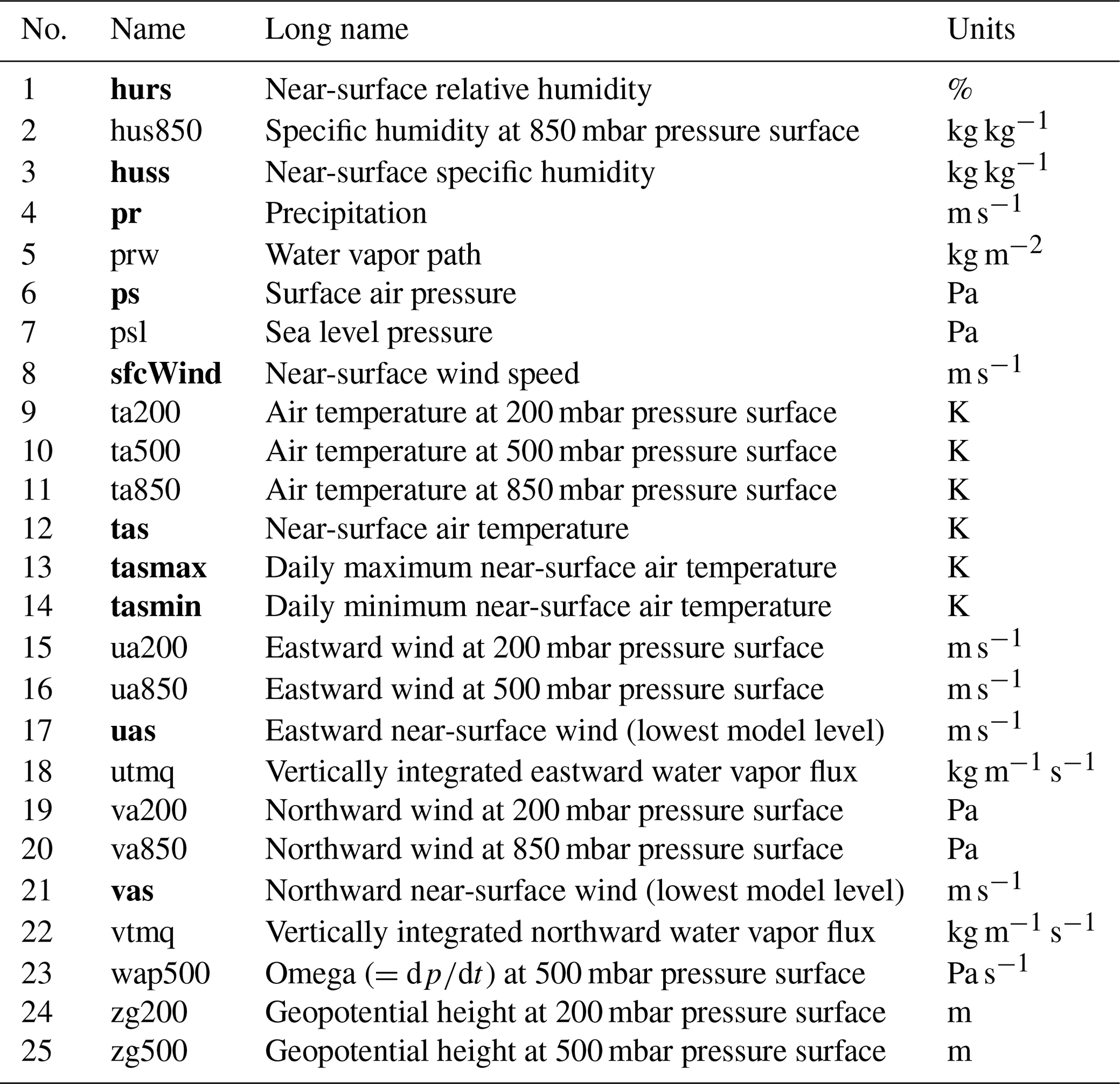
Table C3The 6 h variables. The lowest model level (for uas and vas) is located about 60 m above the surface.
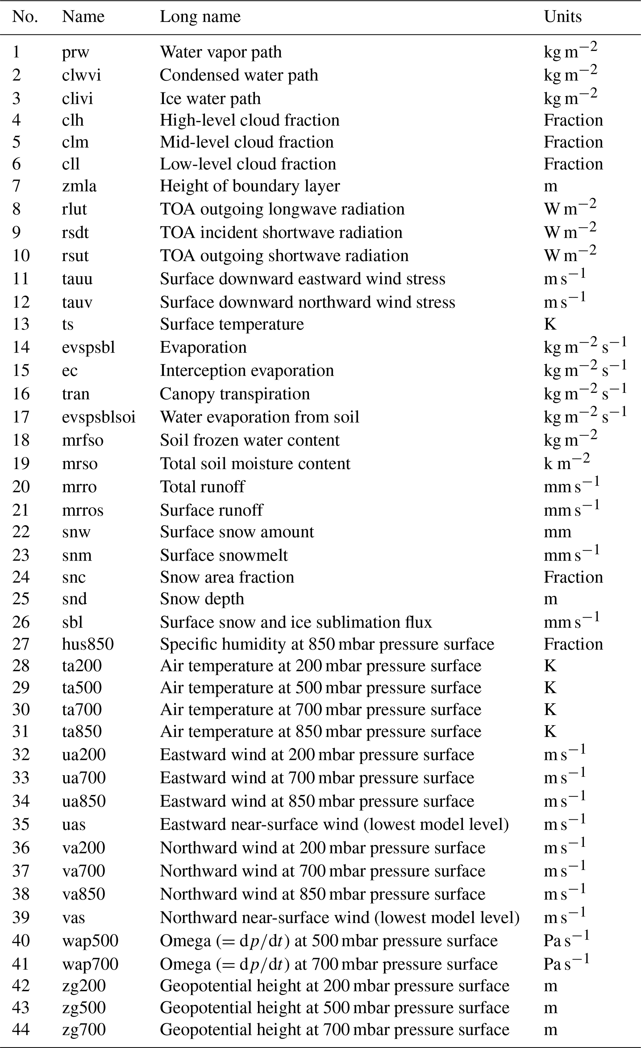
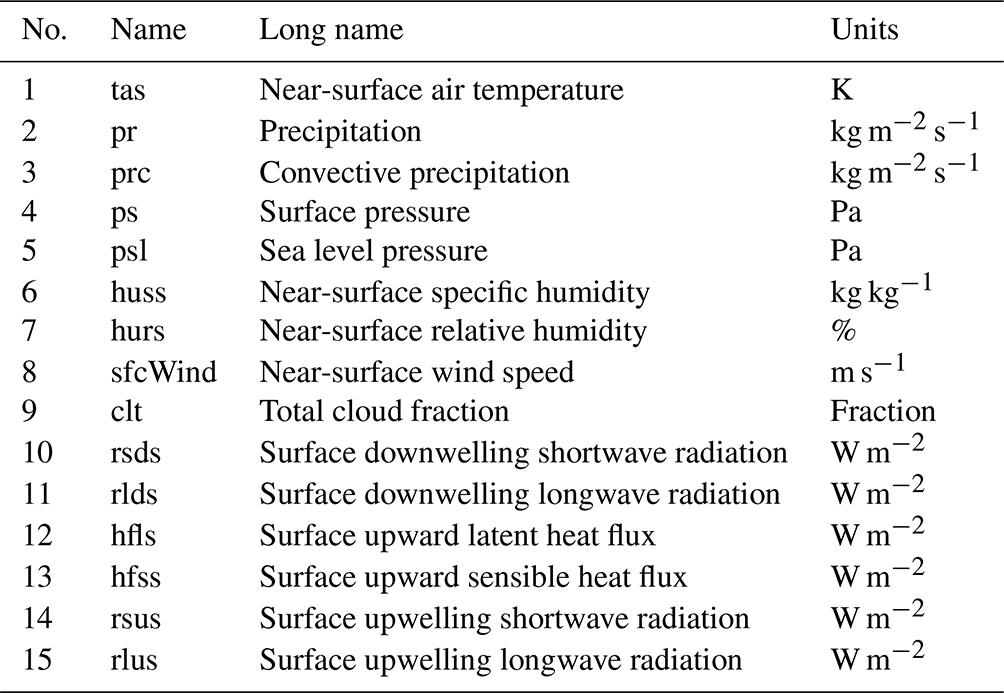
The Cori Haswell (HW) and Edison systems at NERSC feature the same processor family (Intel Xeon processor) on more traditional, massively parallel distributed memory architectures with fewer cores of higher CPU frequencies and larger memory per node. In contrast, Cori Knights Landing (KNL) employs an architecture with a different parallelism philosophy of many cores, wider vector units, and nonuniform and high-bandwidth memory access with the Intel Xeon Phi processors (He et al., 2018). The transition to many-core architecture has occurred in multiple HPC facilities, motivated by better energy efficiency (Allen et al., 2018; Loft, 2020) and preparation of user applications for more extreme many-core architecture with GPU systems (NERSC, 2014).
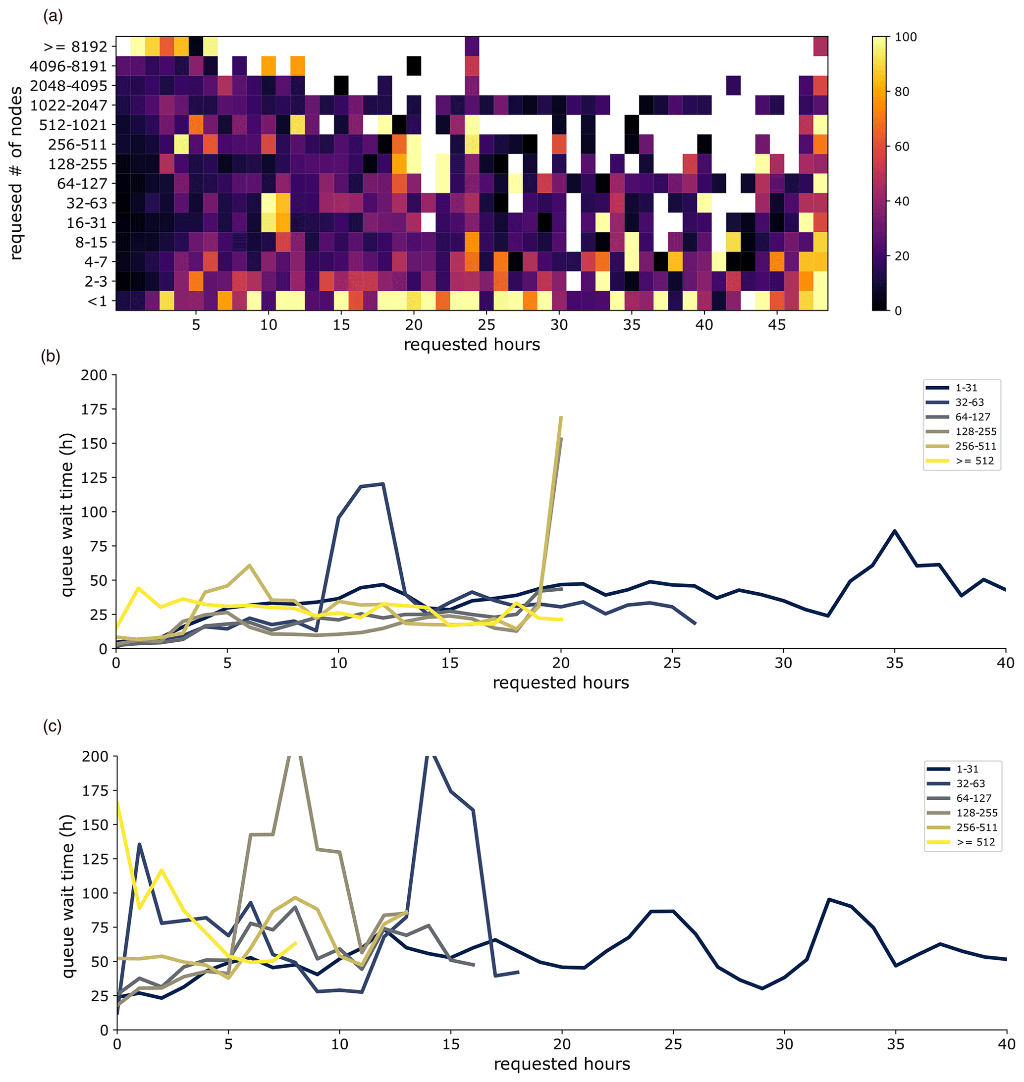
Figure D1The year 2020 annual average queue wait time for (a) Cori KNL as a function of requested wall-clock hours (x axis) and requested number of nodes (y axis). Panel (b) is the same as panel (a) but presents line plots created by further averaging the bins of requested hours to six groups as shown in the legend. Panel (c) is the same as panel (b) but for the Cori HW system. The data were obtained from the MyNERSC website (accessible only by NERSC users) with help from NERSC user support.
To compile the CAM–MPAS code on all of the NERSC systems mentioned above, we use the Intel compiler wrapper provided by the system vendor Hewlett Packard Enterprise Cray (NERSC, 2018). The libraries and compilers that we used can be seen in the “[top directory]/cime/cime_config/cesm/machines/config_machines.xml” file within the source code directory tree. All simulations except for UR120-new use the same model code and same compiler options. We used the O1 compiler optimization level, which is lower than the default for CESM (O2) because the CAM–MPAS code was still an experimental version. UR120-new is run with the beta version of the MPASv6-CESM2 coupled code with the O2 optimization, which can improve simulation throughput by up to ≈10 % compared with O1 based on our benchmark simulations on KNL. Shared-memory parallelism is not used because the MPAS-Atmosphere version 4 does not support OpenMP, and the CESM code does not necessarily show better performance with the hybrid OpenMP–MPI compared with MPI-only configurations (Helen He, personal communication, 2021). For MPI-only jobs, Heinzeller et al. (2016) recommended 100–150 grid columns per MPI task to achieve good throughput for the stand-alone MPAS-Atmosphere model. Not all of our node configurations follow this recommendation for the reasons mentioned below.
At NERSC, queue wait time depends on requested wall-clock hours and number of nodes, but the former tends to be more important than the latter (Fig. D1). Therefore, we aimed for a wall-clock time of 5–6 h or less to integrate 1–6 months in a single job to avoid a long queue wait time. We then looked for sufficient numbers of MPI tasks to achieve this goal to finally determine the number of nodes to request for production simulations. We were also interested in comparing different systems during the transition period from Edison to Cori, so some simulations used similar numbers of nodes or MPI tasks on different systems.
We explored several reasons for the lower throughput of our CAM–MPAS code on Cori KNL than on Cori HW and, especially, the older system Edison. The primary reasons seem to be inefficient memory usage, under-usage of shared-memory parallelism, and source code style that is not easily vectorized by compilers (in addition to the lower level of compiler optimization chosen, as mentioned above). As summarized by He et al. (2018) and Barnes et al. (2017), the previous system Edison has two Intel Ivy Bridge 2.6 GHz 12-core CPUs (24 cores per node) and 64 GB memory with ∼100 GB s−1 bandwidth on each node. Cori KNL, on the other hand, has one Xeon Phi 7250 1.4 GHz processor that has 68 physical cores, each of which can be used with four hardware threads. A KNL node has a larger 96 GB memory with slower 85 GB s−1 bandwidth than Edison but also provides additional 16 GB high-bandwidth (450 GB s−1) memory. Despite the lower clock frequency, KNL's Xeon Phi processor performs 32 double-precision floating-point operations per second (FLOPS) per cycle compared with 8 FLOPS per cycle by Edison's Ivy Bridge processor.
The overall performance of climate model code is typically limited by memory latency and bandwidth rather than arithmetic speed (e.g., Fuhrer et al., 2018; Dennis et al., 2019), except for some components such as the MG2 microphysics (Barnes et al., 2017). A naive use of all 68 cores on KNL nodes as MPI ranks leads to 0.5 GB memory per rank (using KNL's two different memory units as a single entity), which is about one-fifth of the 2.7 GB per rank when using 24 MPI ranks per node on Edison. In addition to this memory-per-rank difference, we found inefficient memory use by the CESM1.5 code, which became clear with very high resolution (more than 1 million columns) but already impacted resolutions with ≈0.5 million grid columns, including the VR12-46 and UR30 grids. An example of inefficient memory use is the storage of unnecessarily long arrays on the memory of each node (e.g., those cover the whole global domain instead of the sub-domain assigned to the MPI rank), which exacerbates less memory per MPI rank on the KNL node.
Recommended programming models for Cori KNL are vectorization, shared-memory parallelism, and control of data block size within the 16 GB high-speed memory. It was found that such programming design is not very common within the CESM code during the NERSC Exascale Science Applications Program (NESAP), which was established to help NERSC users to optimize their applications for KNL (He et al., 2018). As part of the NESAP, two subcomponents of the CESM model were optimized by the code developers and NERSC support staff. The MG2 microphysics code was found to be bounded by computation with poor vectorization, and improved code structure for easier vectorization enhanced its speed by about 75 % (He, 2016; Barnes et al., 2017). Optimizations of the High-Order Method Modeling Environment (HOMME) dynamical core involved both better vectorization and rewriting the OpenMP loops, which together achieved performance that was 2 times faster on KNL (Barnes et al., 2017; Dennis et al., 2019). While some optimizations are more specific to KNL, many of the code changes improve performance on other systems such as the Cheyenne system at the NCAR-Wyoming Supercomputing Center (Dennis et al., 2019).
It is generally difficult for these specific optimizations to be incorporated into the official release of the CESM code (let alone off-branched experimental versions) within the lifetime of a typical HPC system of 4–5 years. This can be a serious and common challenge for climate modeling research groups, whose numerical experiments require long simulation time. Fortunately, the MPAS-Atmosphere code went through several optimizations in version 5, including changes similar to those reported in the above studies. In addition, the memory-scaling issues in the CAM code have been addressed in the current version of CESM2. Along with other numerous changes from CESM1.5 to CESM2.1, the latest version of CAM–MPAS achieves substantially better performance on KNL (Table 5).
This appendix provides additional information for the global climate and its resolution sensitivity in the CAM–MPAS simulations.
E1 Present-day climate biases and resolution sensitivities
As mentioned in the main text (Sect. 5.2.1), the present-day climatology of near-surface air temperature (TAS) is similar across the resolutions (Fig. E1). All of the CAM–MPAS eval simulations share regional biases, most notably the warm bias in the midlatitude continents and in the Southern Hemisphere storm tracks. On the other hand, TAS shows visible difference across resolution over complex terrains such as the Tibetan Plateau and western Americas. Previous studies of the CAM model suggest that the overly warm TAS in the Southern Hemisphere storm track is related to the underestimated low-level liquid clouds (Bogenschutz et al., 2018) and overestimated wind speed (and associated vertical mixing) in the lower atmosphere. For the Arctic region, the CAM5 physics was shown to underestimate Arctic clouds, leading to less downward longwave radiation, smaller surface net energy, and colder surface temperature (English et al., 2014; McIlhattan et al., 2017). Note that the sea-ice model in the CESM AMIP configuration interactively calculates the surface energy balance and temperature given the prescribed ice coverage, unlike the open-ocean surface where the surface skin temperature is prescribed (Sect. 3).
The contour plots of precipitation biases against GPCP show greater variations among simulations than TAS (Fig. E2). UR120 shows the smallest regional bias across the globe, presumably because its grid resolution and time step are close to those of FV1∘, to which we tuned the CAM5.4 physics with the prescribed aerosol scheme (Sect. 2.2).
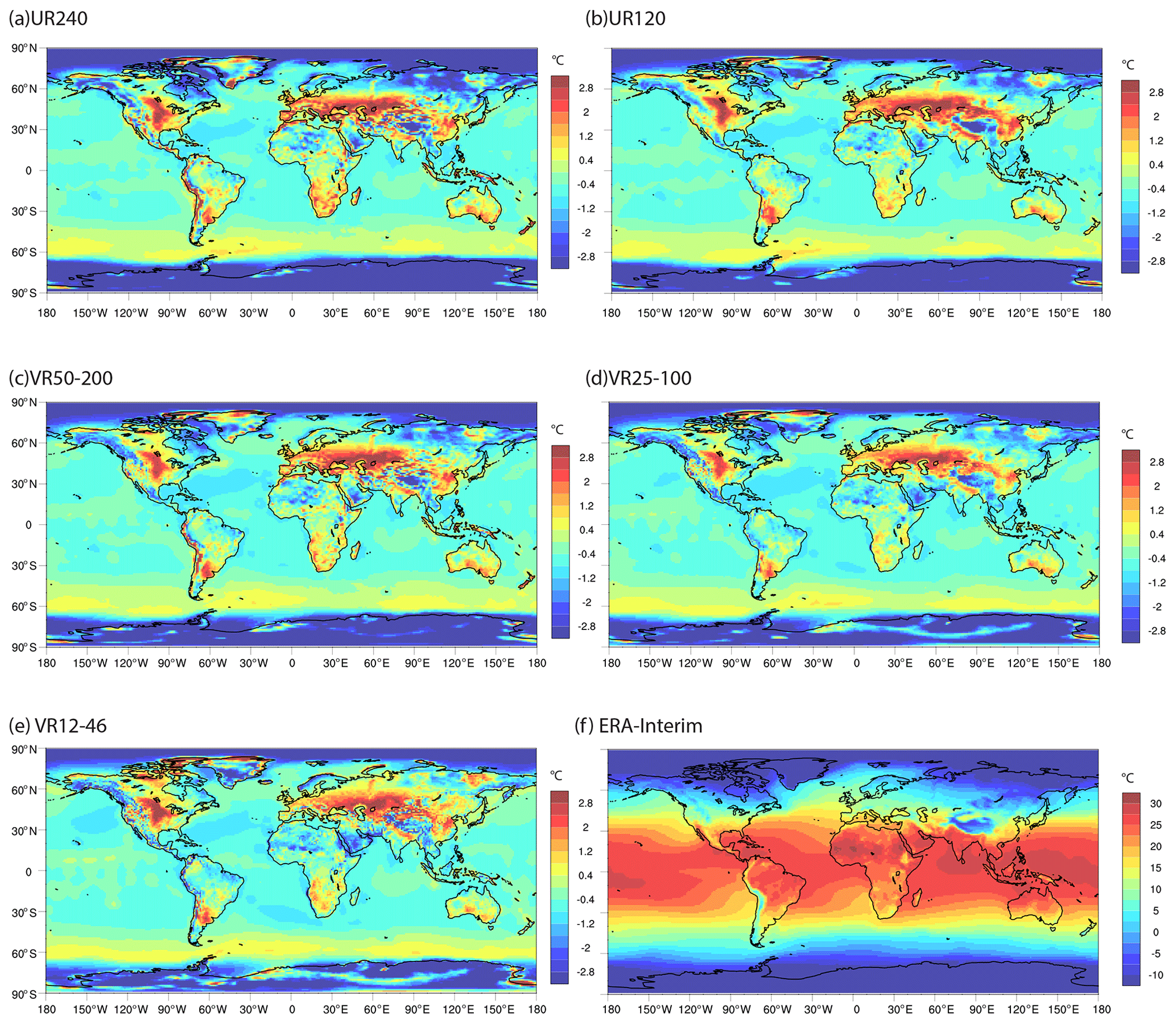
Figure E1Difference in the climatological 2 m air temperature over the 1990–2010 (2001–2010 for VR12-46) period between CAM–MPAS simulations and ERA-Interim (a)–(e) as well as the annual mean temperature in ERA-Interim (f). The ERA-Interim sea surface temperature and sea-ice cover are used as input for the CAM–MPAS AMIP simulations.
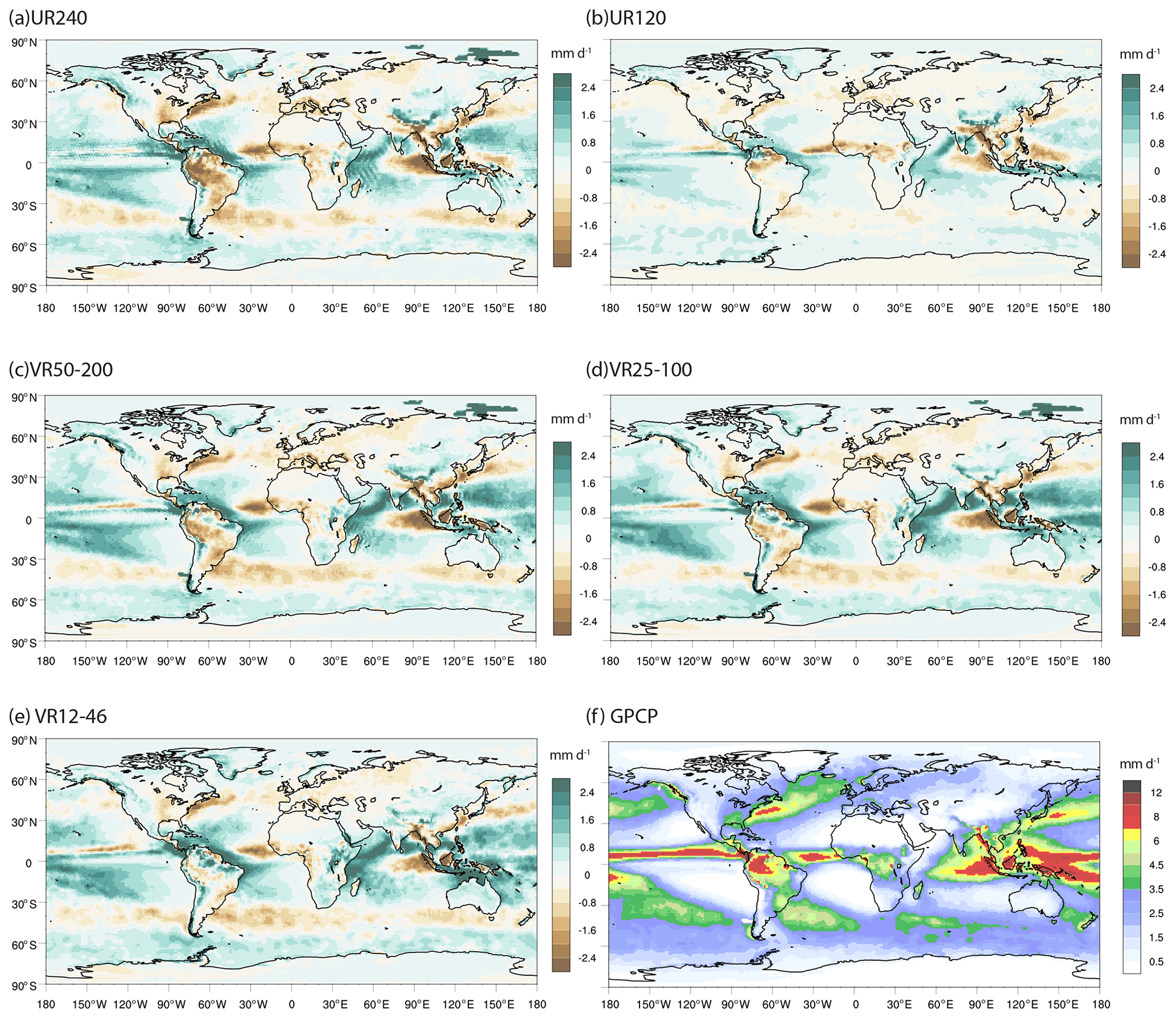
Figure E2Difference in the climatological surface precipitation over the 1997–2010 (2001–2010 for VR12-46) period between CAM–MPAS simulations and GPCP (a)–(e) as well as the annual mean precipitation in GPCP (f). Grid imprinting in the contour plots in panels (a) and (c) over some regions (e.g., the Indian Ocean west of Africa) is a result of conservatively remapping coarser MPAS grids to the finer latitude–longitude grid.
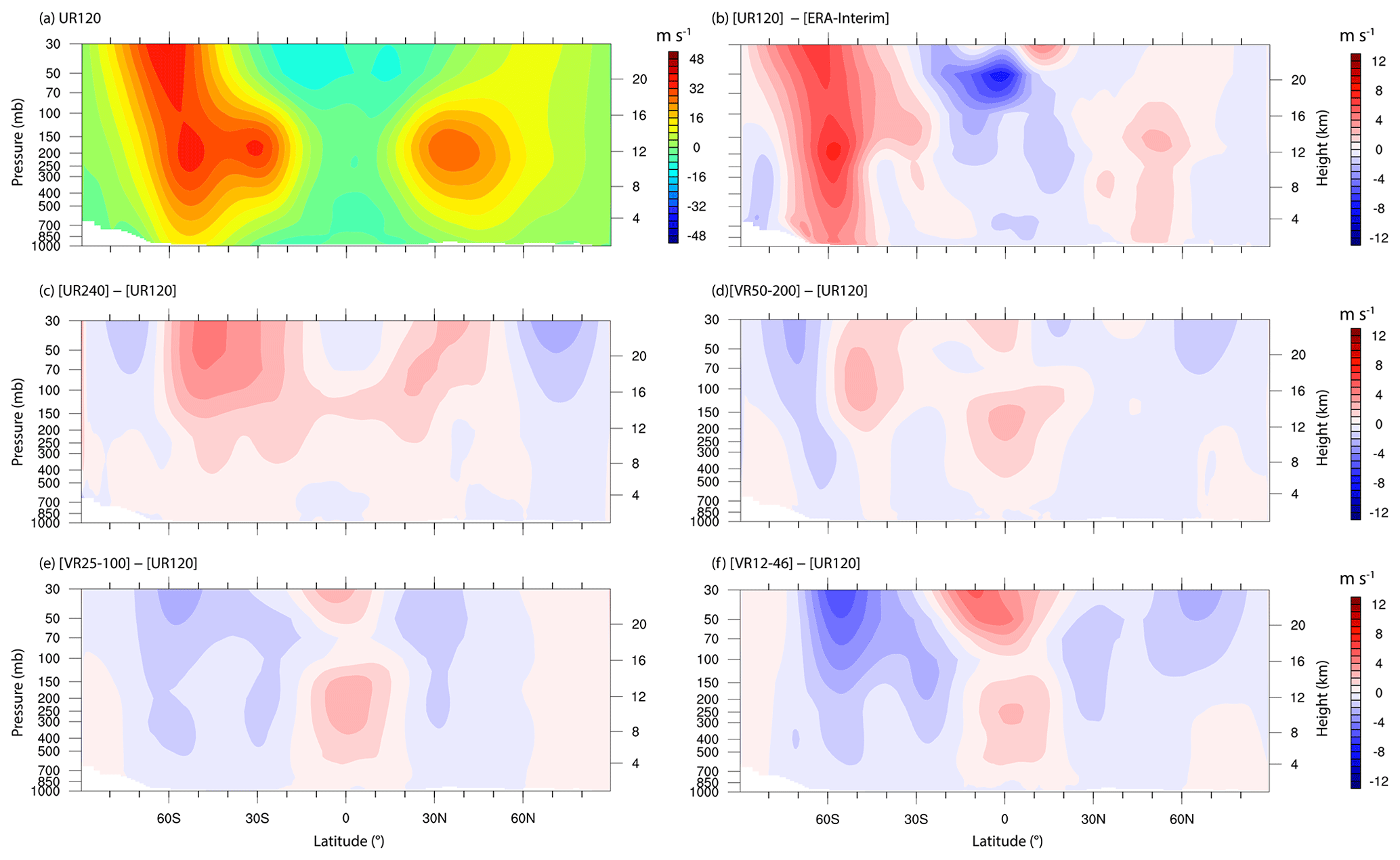
Figure E3Annual climatology of zonal mean zonal wind in (a) UR120, (b) the UR120 bias compared with ERA-Interim, and the differences between UR120 and other CAM–MPAS resolutions, including (c) UR240, (d) VR50-200, (e) VR25-100, and (f) VR12-46.
E2 Future climate changes and resolution sensitivities
Figure E4 compares mean precipitation changes from the historical to RCP8.5 periods in the five CAM–MPAS simulations and the MPI-ESM-LR simulation. As mentioned in the main text, the overall spatial patterns are similar across the simulations. Because the contour color range is set for the larger changes over the ocean, Fig. E5 masks the ocean grid points and focuses on land.
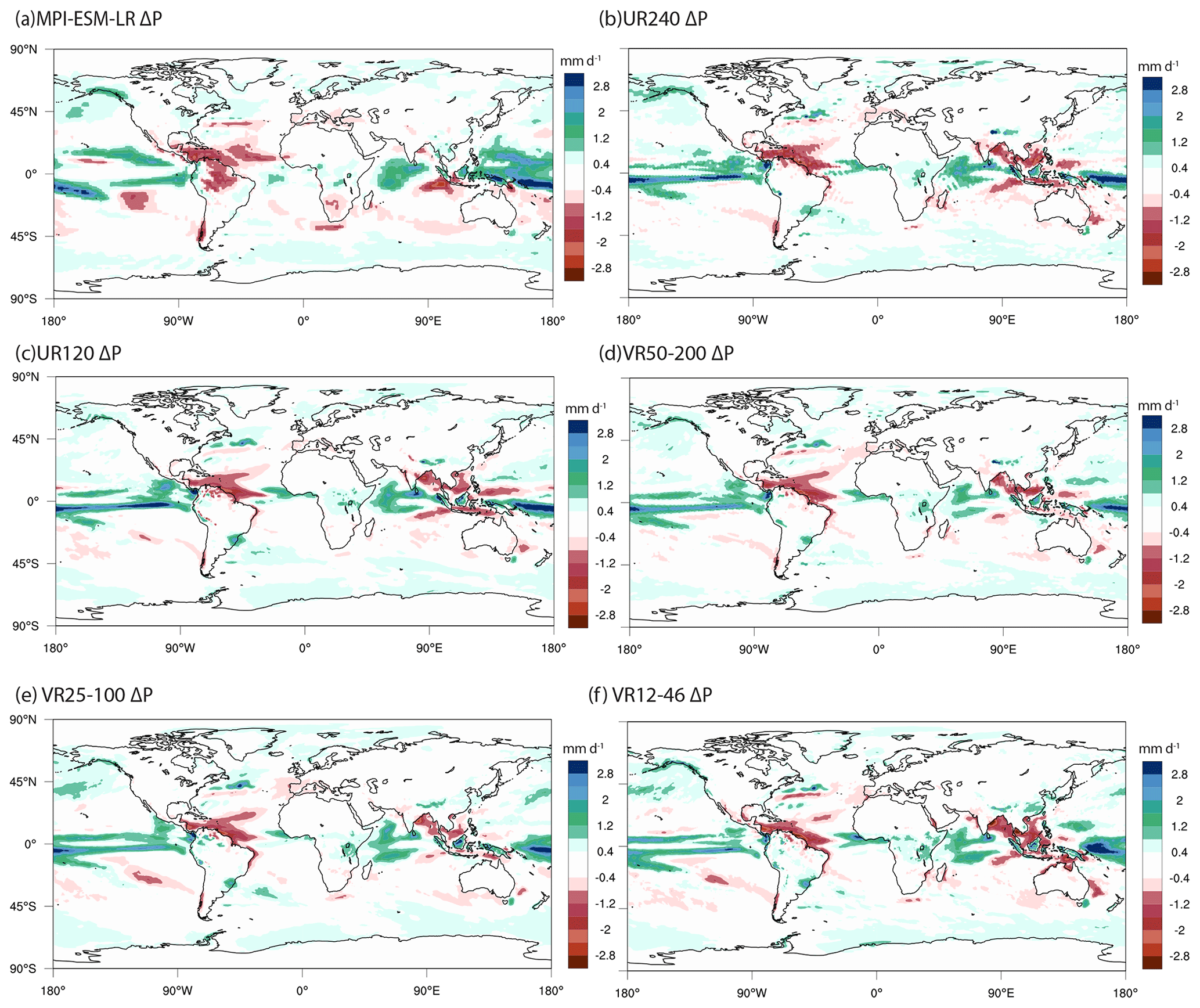
Figure E4Projected precipitation change from the historical to RCP8.5 periods in (a) MPI-ESM-LR, (b) UR240, (c) UR120, (d) VR50-200, (e) VR25-100, and (f) VR12-46.
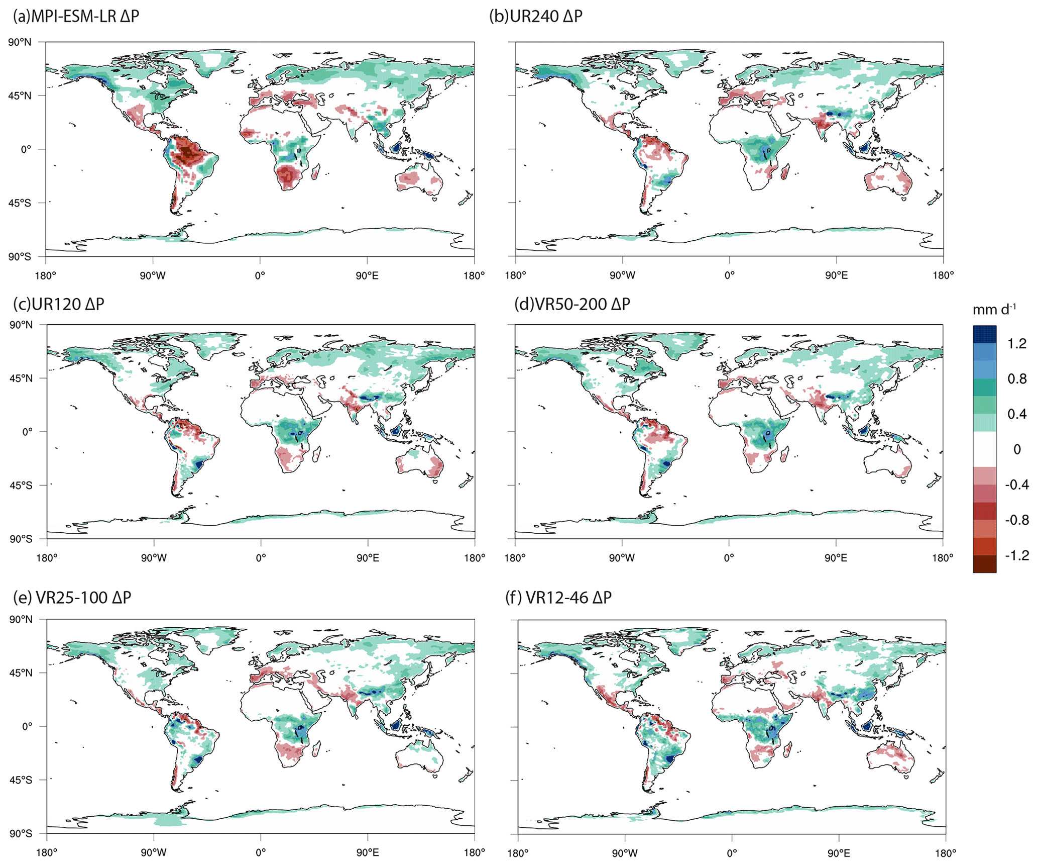
Figure E5Same as Fig. E4 but the ocean grid points are masked and a narrower color range is used to focus on precipitation change over land.
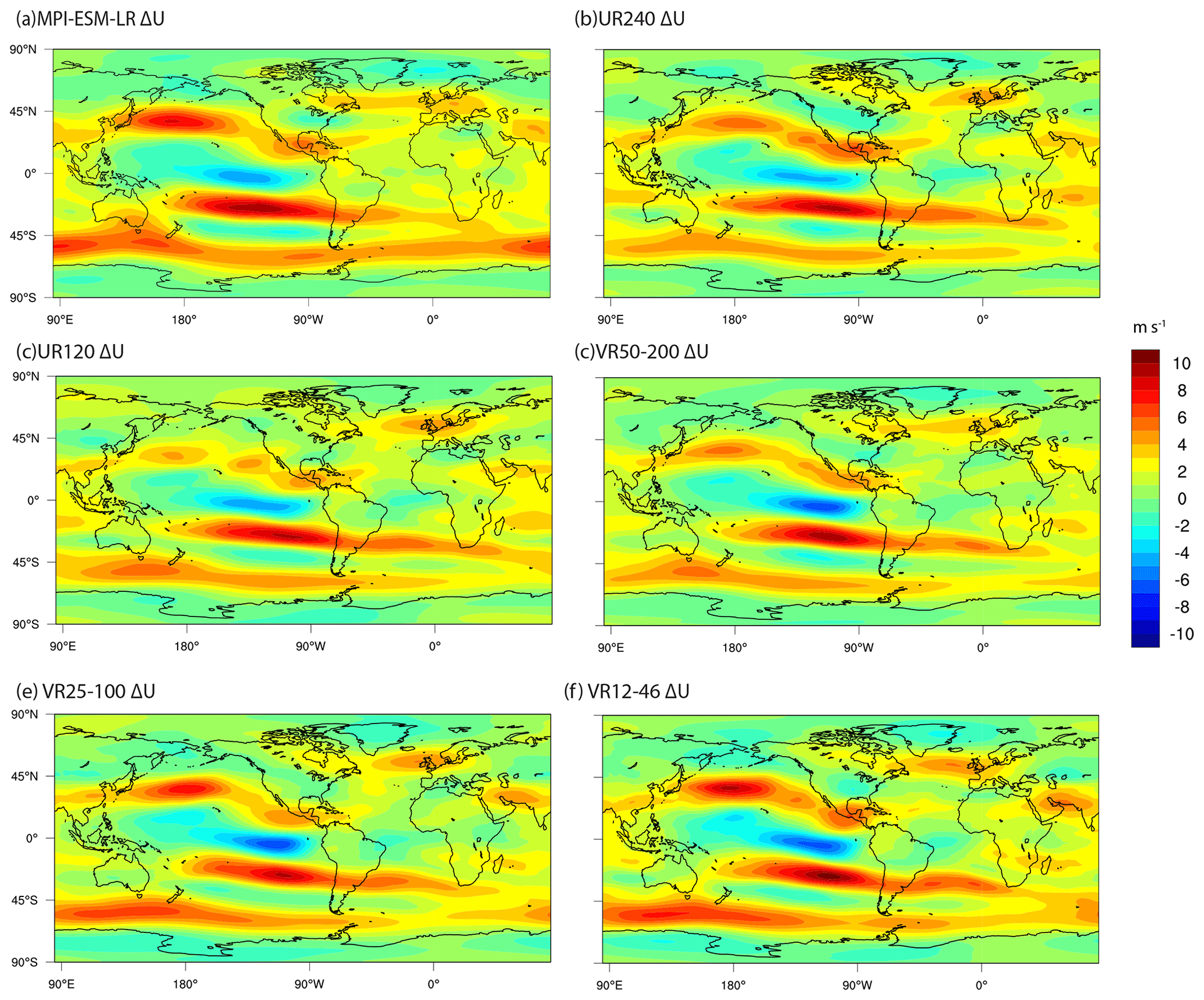
Figure E6Same as Fig. E4 but for the projected change in zonal wind at the 200 hPa level (ΔUA200).
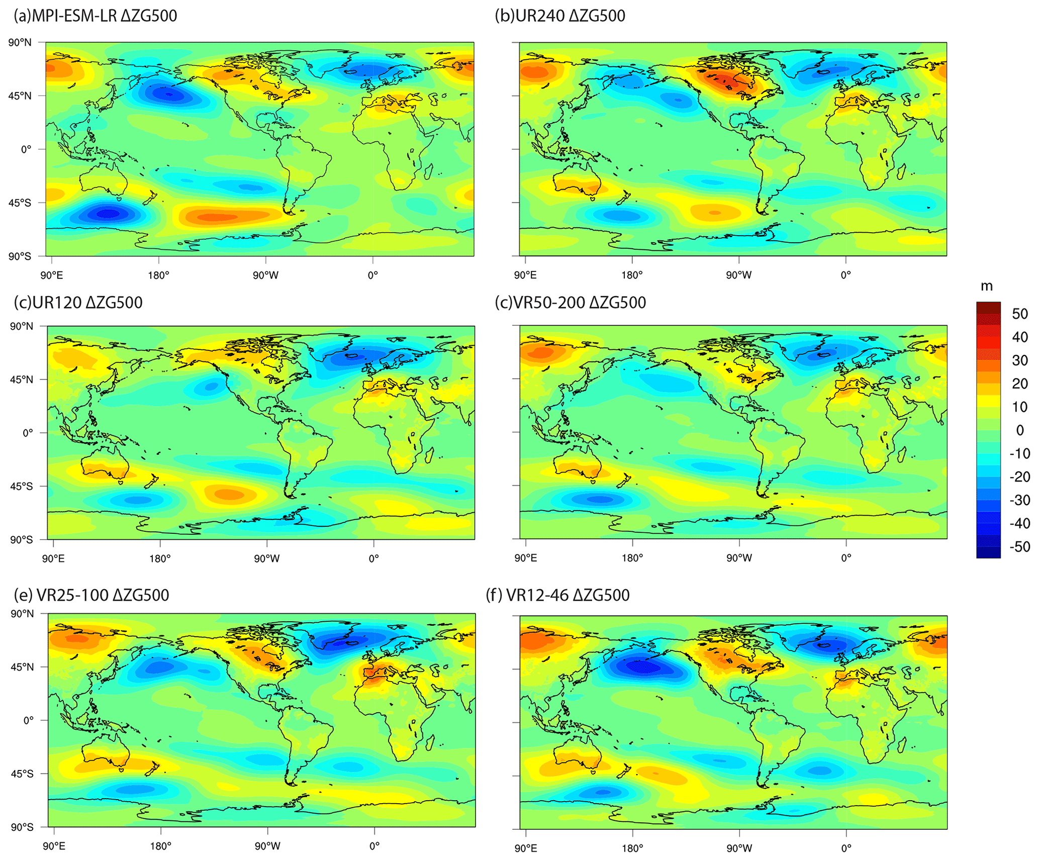
Figure E7Same as Fig. E4 but for the projected change in the zonal anomaly of the geopotential height at the 500 hPa level (ΔZG500).
Table E1Observational datasets used in Table 6 and their references, obtained through Atmospheric Model Working Group (2014).
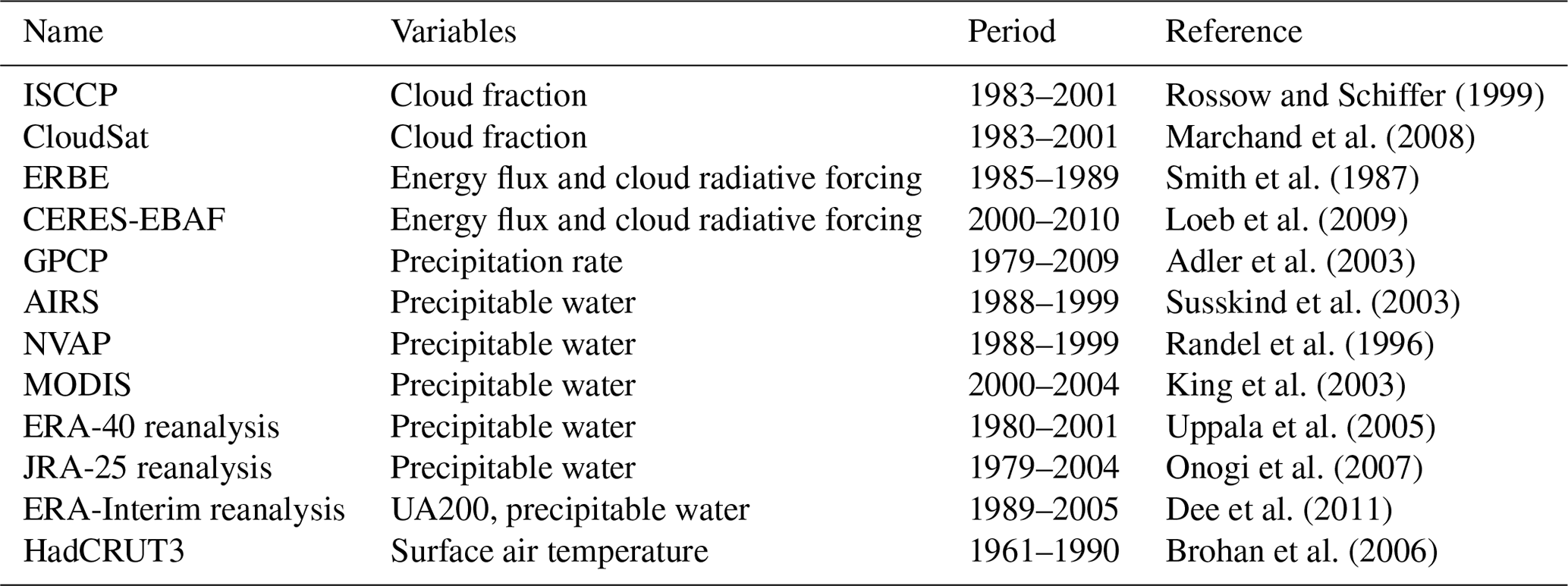
This appendix provides an overview of the regional climate evaluated over CONUS (defined as 30–47∘ N, 105–85∘ W) and its resolution sensitivity in the CAM–MPAS simulations.
The time series of annual and regional mean near-surface air temperature (TAS) over the CONUS region is nearly identical among the different resolutions (Fig. F1a, b), except for some seasonal maxima and minima where significant differences can arise in some years. The TAS spatial patterns, shown as differences from the ERA-Interim temperature in Fig. F2, illustrate that the spatial patterns of the biases (and TAS itself) are also similar across simulations over the central and eastern US. Over the western US, with complex surface topography, greater spatial variability is simulated by finer spatial resolutions. The topography-related spatial variability seems to be filtered out and does not affect the regional average time series.
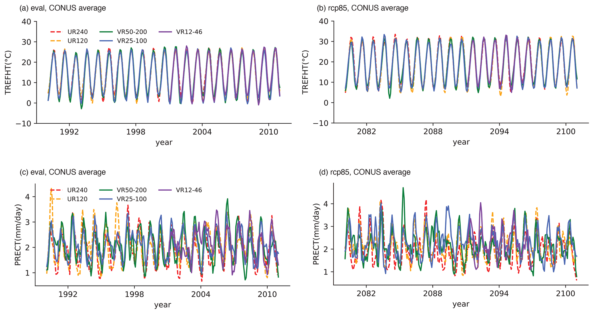
Figure F1Time series of monthly average (a) near-surface air temperature in the present-day (eval) simulations, (b) near-surface air temperature in the future (rcp85) simulations, (c) precipitation in the present-day (eval) simulations, and (d) precipitation in the future (rcp85) simulations. All variables are averaged over the CONUS domain defined as 30–47∘ N, 85–105∘ W.
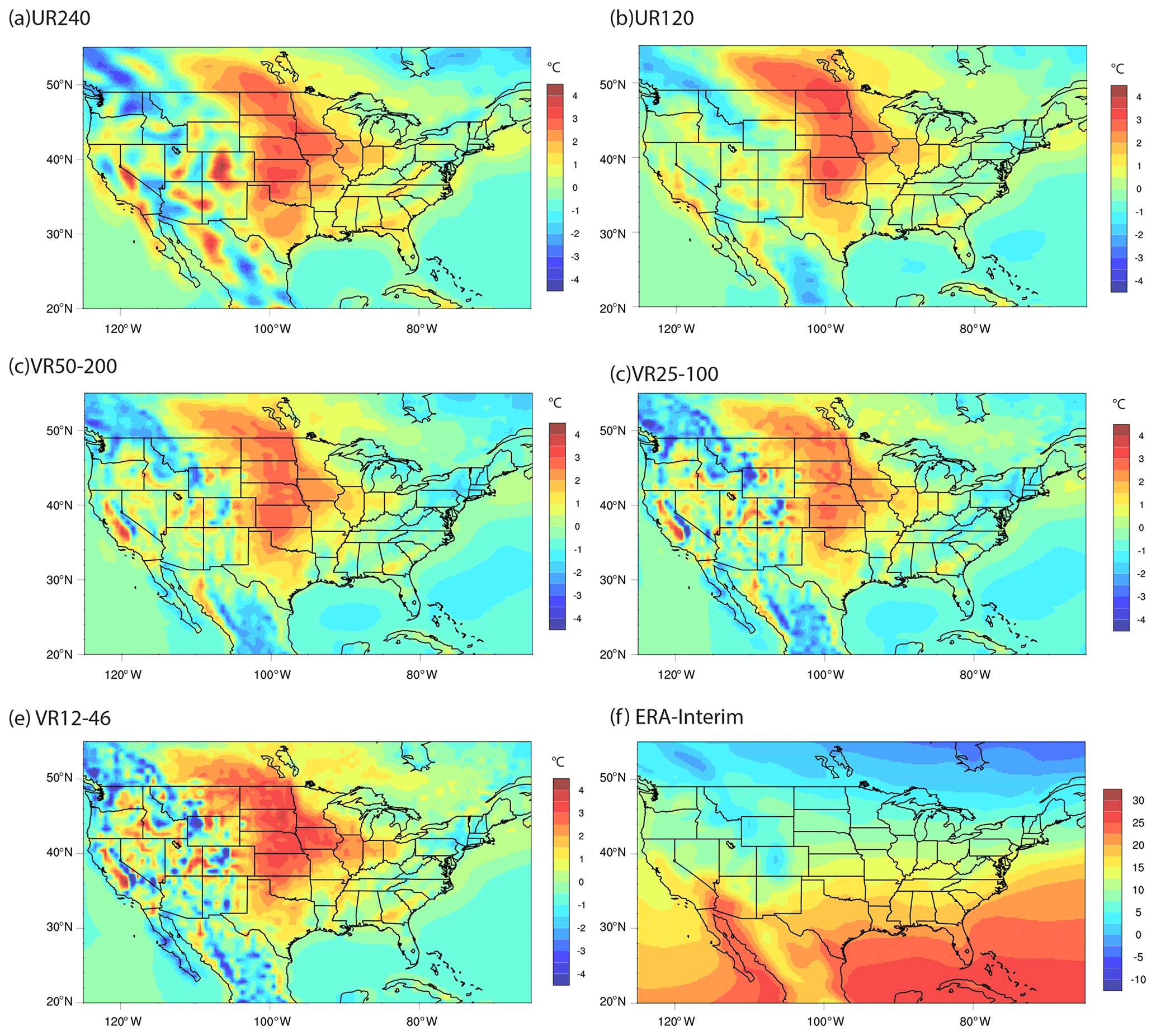
Figure F2Annual mean 2 m air temperature bias as in Fig. E1 but showing only the CONUS region. Panel (f) is not the bias but rather the mean surface temperature from ERA-Interim.
The CONUS-averaged precipitation, on the other hand, varies significantly across years and among resolutions (Fig. F1c, d). The resolution sensitivity of the CONUS-averaged precipitation is not as simple or systematic as the global mean precipitation. A subtle but consistent increase with resolution appears in the total (combined convective and large-scale) precipitation after further averaging over time, but it is not seen in individual convective and large-scale components (Table F1). As in TAS, the spatial patterns of precipitation bias are similar across simulations over the central and eastern US, but greater variability appears with higher resolution over the western US (Fig. F3).
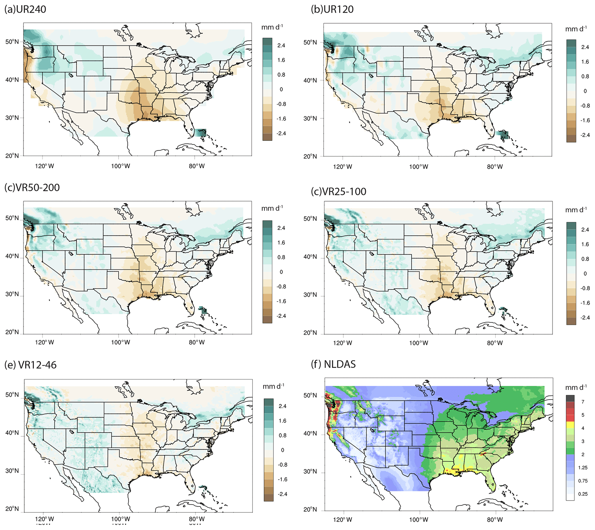
Figure F3Annual mean precipitation bias as in Fig. E1 but showing only the CONUS region and using North American Land Data Assimilation System (NLDAS) data instead of GPCP as a reference in panel (f).
An interesting difference between the TAS and precipitation biases is that the TAS warm bias is maximized over the northern central US (35–55∘ N) and shows little sensitivity to resolution, whereas the precipitation dry bias is greatest in the southern central US (30–35∘ N) and does show sensitivity to resolution. Multiple performance metrics – the ratio of spatial variance, mean bias, and centered (i.e., mean bias already removed) root-mean-square error (CRMSE) – calculated over the CONUS region suggest that surface precipitation is best simulated by VR12-46 (Fig. F4b). Comparing all resolutions, both the spatial variability (variance ratio and centered RMSE) and the mean (normalized bias) of precipitation are better simulated by finer resolution. On the other hand, the correlation and variance ratio for TAS depend more weakly on resolution (Fig. F4a).
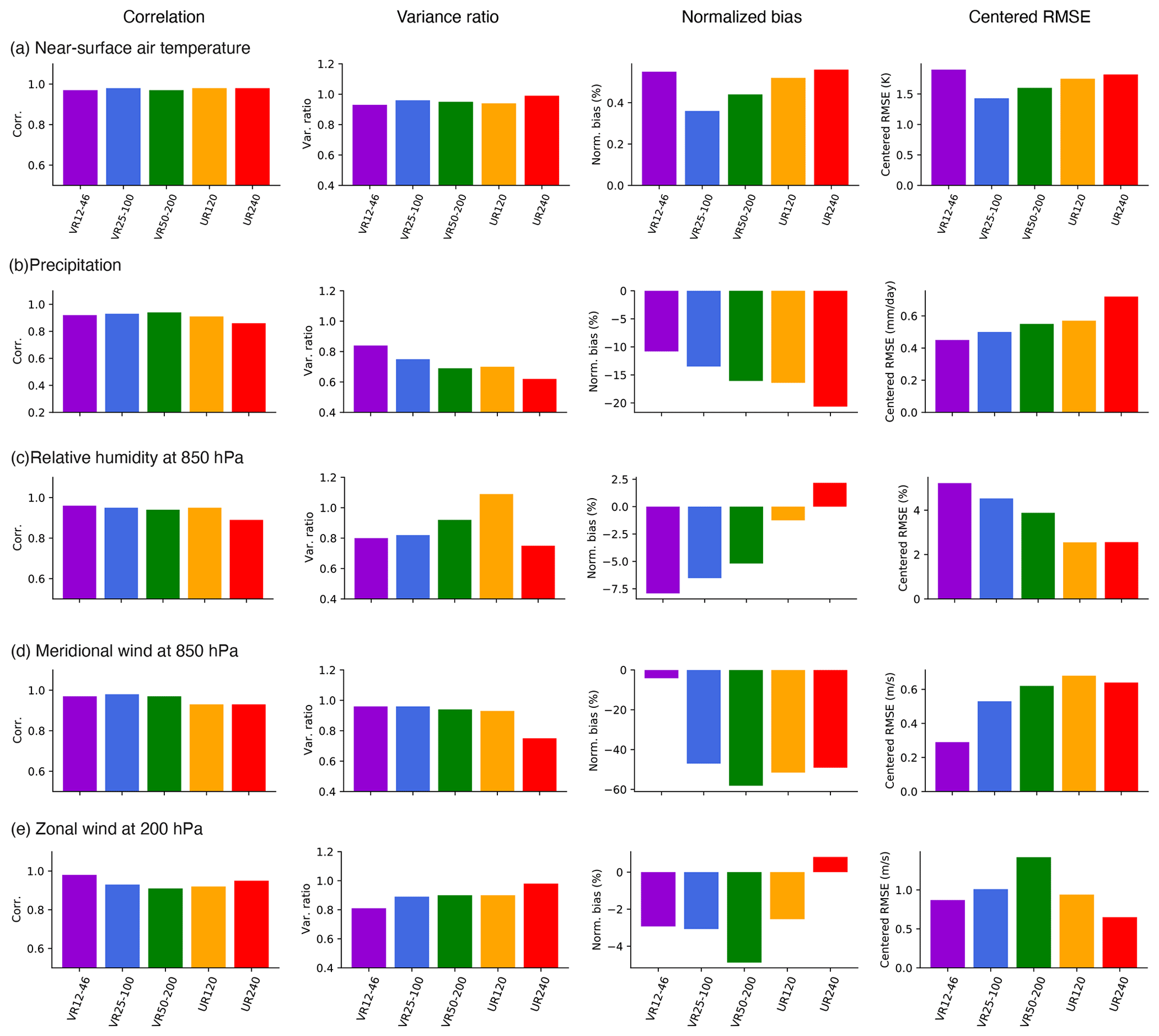
Figure F4Model error metrics calculated over the CONUS region for (a) near-surface temperature, (b) precipitation, (c) relative humidity at 850 hPa, (d) meridional wind at 850 hPa, and (e) zonal wind at 200 hPa. Annual averages for the years 1990–2010 (2000–2010 for VR12-46) from NLDAS are used as a reference for precipitation, and those from ERA-Interim are used for other variables. Four error metrics (columns) are presented: (1) the linear correlation of spatial patterns (Corr.); (2) the ratio of the spatial variance (, where the subscripts “ref” and “mod” refer to the reference data and model, respectively); (3) the normalized bias (%) (, where the overbar denotes the regional average); and (4) the centered RMSE, which is a RMSE calculated after the regional averages are removed.
Other hydrological components show more consistent resolution sensitivities than the surface precipitation. For example, the regional average cloud cover and low-level humidity become progressively smaller with higher resolution (Table F1). The resolution sensitivity is more subtle for large-scale forcing terms such as relative humidity and meridional winds at the 850 hPa level (denoted as RH850 and VA850, respectively) and zonal wind at the 200 hPa level (UA200), which have been suggested to be important for the regional hydrological cycle over CONUS (e.g., Bukovsky et al., 2017; Song et al., 2019). Compared with ERA-Interim, VA850 metrics improve with finer resolution (Fig. F4c). In contrast, UA200 and RH850 do not show similar improvement with increasing spatial resolution. A lack of coherent resolution sensitivity of UA200 is consistent with Fig. E3 where little difference is seen between the simulations in the Northern Hemisphere midlatitudes.
As we prepare a more detailed documentation of the regional climate simulations, we refer potential data users to the following studies evaluating the aspects of the CAM–MPAS simulations not documented here. Feng et al. (2021) performed in-depth analysis of the simulated precipitation over CONUS, focusing on the mesoscale convective systems (MCSs) and associated large-scale environment. They found that the model is capable of simulating the large-scale meteorological patterns favorable for producing MCSs identified from the observed MCS database but at lower frequency, leading to an underestimation of the MCS number. They concluded that the incorrect response of moist (deep-convection) parameterizations to the large-scale environment is likely the main reason for the bias. Pryor et al. (2020) compared the present-day and future simulations by WRF and CAM–MPAS in terms of the mean annual energy density from the wind turbines derived from the near-surface wind speed, noting significantly weaker near-surface winds in CAM–MPAS than WRF. Their sensitivity test indicates the overestimated drag from the turbulent mountain stress parameterization in CAM5, also reported by Lindvall et al. (2013). Because model biases are largely inherited from the CAM5.4 parameterizations, previous studies using the CAM5 physics with VR approach are also useful to understand the model behavior (Huang et al., 2016; Rhoades et al., 2016, 2018b; Gettelman et al., 2018).
Table F1Climatological means of selected variables over CONUS from present-day (eval) simulations.
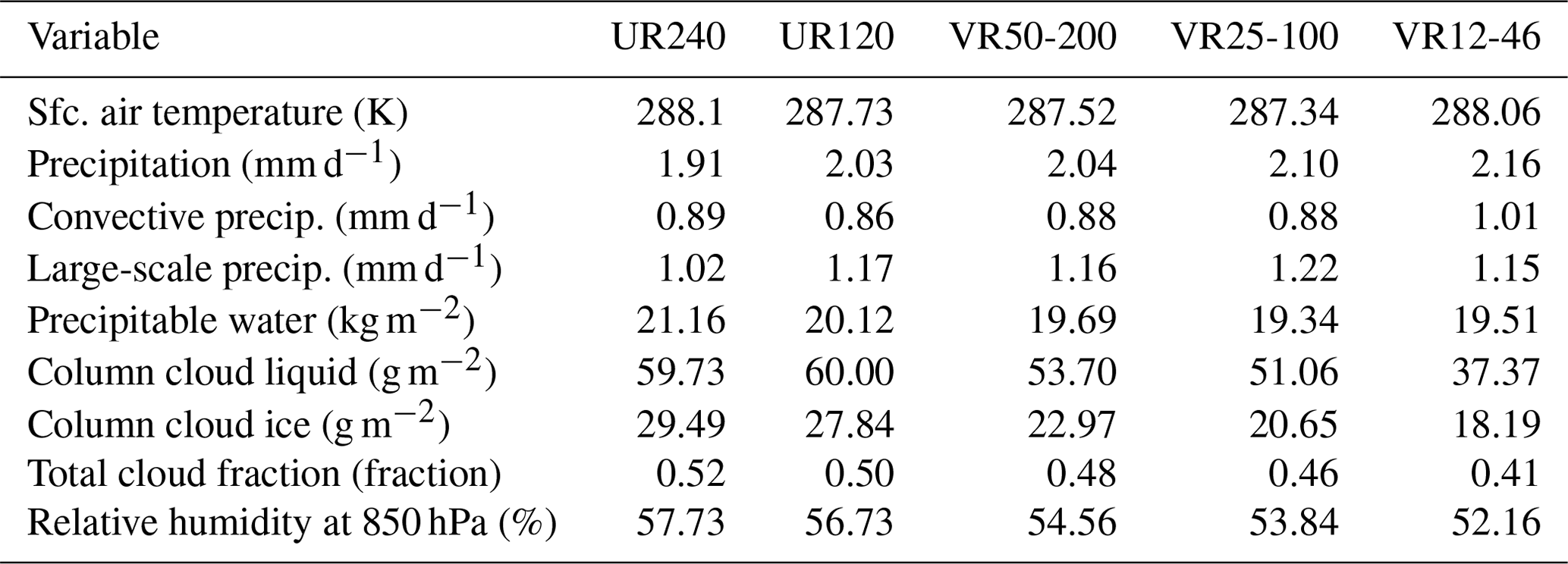
Table F2Examples of the number of grid columns in the regional model simulations from the NA-CORDEX and FACETS archives.
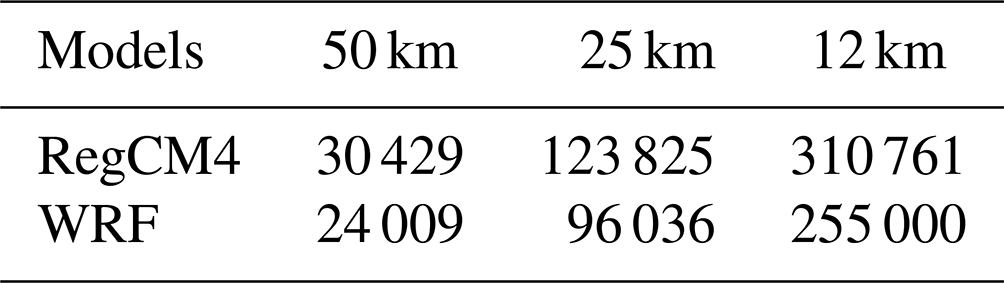
Post-processed monthly variables and a subset of daily variables (essential and high priority categories in the NA-CORDEX archive) are available from the Pacific Northwest National Laboratory DataHub (Sakaguchi et al., 2022) (https://doi.org/10.25584/PNNL.data/1895153). All of the post-processed and raw model output is available from the NERSC High Performance Storage System (HPSS) through the NERSC Science Gateway Service (https://portal.nersc.gov/archive/home/k/ksa/www/FACETS/CAM-MPAS, Sakaguchi, 2023).
The official version of the CESM model is available as a public-domain software from the project website (https://www.cesm.ucar.edu/models/, Sacks et al., 2020). The particular version of the experimental CAM–MPAS code used for this study is archived on Zenodo (Sakaguchi and Harrop, 2022) (https://doi.org/10.5281/zenodo.7262209). A set of input data files to reproduce the simulations reported here is also available on Zenodo (Sakaguchi, 2022) (https://doi.org/10.5281/zenodo.7490129).
KS, LRL, WJG, and LM designed the experiments and KS carried them out. SM guided post-processing of the MPAS output in accordance with the NA-CORDEX protocol. CMZ, WCS, and CZ contributed to porting the MPAS model into the CESM code. KS, CMZ, JJ, BEH, WCS, and AG regularly participated in monthly meetings to provide feedback on technical and scientific problems. CMZ, JJ, WCS, AG, and CZ provided further help with respect to solving technical problems. SL provided high-performance computing support for the simulations and helped with obtaining usage data from the National Energy Research Scientific Computing Center systems. KS prepared the paper with contributions from LRL, JJ, SM, BEH, WCS, WJG, and SL.
The contact author has declared that none of the authors has any competing interests.
Publisher’s note: Copernicus Publications remains neutral with regard to jurisdictional claims in published maps and institutional affiliations.
We acknowledge the financial support from the US Department of Energy, Office of Science, Office of Biological and Environmental Program through the following projects: “A Hierarchical Evaluation Framework for Assessing Climate Simulations Relevant to the Energy–Water–Land Nexus (FACETS)”, “A Framework for Improving Analysis and Modeling of Earth System and Intersectoral Dynamics at Regional Scales (HyperFACETS)”, and the “Water Cycle and Climate Extremes Modeling (WACCEM)” scientific focus area. Chun Zhao was supported by the USTC Research Funds of the Double First-Class Initiative and the Strategic Priority Research Program of Chinese Academy of Sciences. We also acknowledge the technical contributions of Michael Duda, Sang-Hun Park, and Peter Lauritzen to the CAM–MPAS code. This research used resources of the National Energy Research Scientific Computing Center (NERSC), a US Department of Energy Office of Science User Facility operated under contract no. DE-AC02-05CH11231. Advice from the NERSC user support regarding resolving technical issues was greatly appreciated. The following software was used for processing model input and output data: netCDF Operators (NCO) version 4.7.0 (Zender, 2017), NCAR Command Language (NCL) version 6.4 (UCAR/NCAR/CISL/TDD, 2017), GNU Parallel (Tange, 2018), and TaskFarmer (NERSC, https://docs.nersc.gov/jobs/workflow/taskfarmer/ (last access: 18 May 2023). Lastly, the authors thank the anonymous reviewers and the editor for their thorough review and suggestions that improved the clarity and fidelity of the paper.
This work has been funded by the US Department of Energy, Office of Science, Office of Biological and Environmental Research program under award no. DE-SC0016438 “A Hierarchical Evaluation Framework for Assessing Climate Simulations Relevant to the Energy–Water–Land Nexus (FACETS)” as well as award no. DE-SC0016605 “A Framework for Improving Analysis and Modeling of Earth System and Intersectoral Dynamics at Regional Scales (HyperFACETS)” as part of the Regional and Global Model Analysis (RGMA) and MultiSector Dynamics (MSD) program areas. Some data analysis and collaborative work has also been supported by the RGMA program area through the Water Cycle and Climate Extremes Modeling (WACCEM) scientific focus area under grant no. 68949. Moreover, this work received funding from the Research Funds of the Double First-Class Initiative, University of Science and Technology of China (grant no. YD2080002007) and the Strategic Priority Research Program of Chinese Academy of Sciences (grant no. XDB41000000).
This paper was edited by Sophie Valcke and reviewed by two anonymous referees.
Adler, R. F., Huffman, G. J., Chang, A., Ferrado, R., Xie, P.-P., Janowiak, J., Rudolf, B., Schneider, U., Curtis, S., Bolvin, D. T., Gruber, A., Susskind, J., Arkin, P., and Nelkin, E.: The Version-2 Global Precipitation Climatology Project (GPCP) monthly precipitation analysis (1979 – Present), J. Hydrometeorol., 4, 1147–1167, 2003. a
Allen, T., Daley, C. S., Doerfler, D., Austin, B., and Wright, N. J.: Performance and energy usage of workloads on KNL and haswell architectures, Lecture Notes in Computer Science (including subseries Lecture Notes in Artificial Intelligence and Lecture Notes in Bioinformatics), 10724 LNCS, 236–249, https://doi.org/10.1007/978-3-319-72971-8_12, 2018. a
Atmospheric Model Working Group: Atmospheric Model Working Group (AMWG) diagnostics package, Subversion Repository [code], https://www2.cesm.ucar.edu/working_groups/Atmosphere/amwg-diagnostics-package/index.html (last access: 18 May 2023), 2014. a, b
Atmosphere Model Working Group: CAM5.4: Final configuration AMWG diagnostic package, https://webext.cgd.ucar.edu/FAMIP/f.e13.FAMIPC5.f09_f09_beta17_cam5.4_alpha03.002/atm/f.e13.FAMIPC5.f09_f09_beta17_cam5.4_alpha03.002-obs/ (last access: 13 May 2023), 2015. a, b, c
Bacmeister, J. T., Wehner, M. F., Neale, R. B., Gettelman, A., Hannay, C., Lauritzen, P. H., Caron, J. M., and Truesdale, J. E.: Exploratory high-resolution climate simulations using the Community Atmosphere Model (CAM), J. Climate, 27, 3073–3099, https://doi.org/10.1175/JCLI-D-13-00387.1, 2014. a, b, c
Balaji, V., Boville, B., Cheung, S., Collins, N., Cruz, C., Silva, A., Deluca, C., Fainchtein, R. D., Eaton, B., Hallberg, B., Henderson, T., Hill, C., Iredell, M., Jacob, R., Jones, P., Kluzek, E., Kauffman, B., Larson, J., Li, P., Liu, F., Michalakes, J., Murphy, S., Neckels, D., Kuinghttons, R. O., Oehmke, B., Panaccione, C., Rosinski, J., Sawyer, W., Schwab, E., Smithline, S., Spector, W., Stark, D., Suarez, M., Swift, S., Theurich, G., Trayanov, A., Vasquez, S., Wolfe, J., Yang, W., Young, M., and Zaslavsky, L.: Earth System Modeling Framework ESMF Reference Manual for Fortran Version 7.1.0r, Tech. rep., The Earth System Modeling Framework, https://earthsystemmodeling.org/docs/release/ESMF_7_1_0r/ESMF_refdoc.pdf (last access: 18 May 2023), 2018. a, b, c
Barnes, T., Cook, B., Deslippe, J., Doerfler, D., Friesen, B., He, Y., Kurth, T., Koskela, T., Lobet, M., Malas, T., Oliker, L., Ovsyannikov, A., Sarje, A., Vay, J. L., Vincenti, H., Williams, S., Carrier, P., Wichmann, N., Wagner, M., Kent, P., Kerr, C., and Dennis, J.: Evaluating and optimizing the NERSC workload on knights landing, Proceedings of PMBS 2016: 7th International Workshop on Performance Modeling, Benchmarking and Simulation of High Performance Computing Systems – Held in conjunction with SC 2016: The International Conference for High Performance Computing, Networking, St, Salt Lake City, UT, USA, 14–14 November 2016, 43–53, https://doi.org/10.1109/PMBS.2016.010, 2017. a, b, c, d, e
Bogenschutz, P. A., Gettelman, A., Hannay, C., Larson, V. E., Neale, R. B., Craig, C., and Chen, C.-C.: The path to CAM6: coupled simulations with CAM5.4 and CAM5.5, Geosci. Model Dev., 11, 235–255, https://doi.org/10.5194/gmd-11-235-2018, 2018. a, b, c
Bretherton, C. S. and Park, S.: A New Moist Turbulence Parameterization in the Community Atmosphere Model, J. Climate, 22, 3422–3448, https://doi.org/10.1175/2008JCLI2556.1, 2009. a
Brohan, P., Kennedy, J. J., Harris, I., Tett, S. F. B., and Jones, P. D.: Uncertainty estimates in regional and global observed temperature changes: A new data set from 1850, J. Geophys. Res., 111, D12106, https://doi.org/10.1029/2005JD006548, 2006. a
Bukovsky, M. S., McCrary, R. R., Seth, A., and Mearns, L. O.: A mechanistically credible, poleward shift in warm-season precipitation projected for the U.S. Southern Great Plains?, J. Climate, 30, 8275–8298, https://doi.org/10.1175/JCLI-D-16-0316.1, 2017. a, b
CESM: CCSM4 half-degree runs, https://www.earthsystemgrid.org/dataset/ucar.cgd.ccsm4.CCSM4-HDEG.html (last access: 19 May 2023), 2016. a
CESM Software Engineering Group: CESM1.2 User Guide, https://www.cesm.ucar.edu/models/cesm1.2/cesm/doc/usersguide/book1.html (last access: 19 May 2023), 2014. a, b, c, d
Chang, H.-i., Castro, C. L., Carrillo, C. M., and Dominguez, F.: The more extreme nature of U.S. warm season climate in the recent observational record and two “well‐performing” dynamically downscaled CMIP3 models, J. Geophys. Res.-Atmos., 120, 8244–8263, https://doi.org/10.1002/2015JD023333, 2015. a
Chen, C. T. and Knutson, T.: On the verification and comparison of extreme rainfall indices from climate models, J. Climate, 21, 1605–1621, https://doi.org/10.1175/2007JCLI1494.1, 2008. a
Christensen, O. B., Gutowski, W. J., Nikulin, G., and Legutke, S.: CORDEX Archive Design, Tech. Rep. March, CORDEX, https://is-enes-data.github.io/cordex_archive_specifications.pdf (last access: 18 May 2023), 2014. a
Christenson, C. E., Martin, J. E., and Handlos, Z. J.: A synoptic climatology of Northern Hemisphere, cold season polar and subtropical jet superposition events, J. Climate, 30, 7231–7246, https://doi.org/10.1175/JCLI-D-16-0565.1, 2017. a
Coburn, J. and Pryor, S. C.: Differential Credibility of Climate Modes in CMIP6, J. Climate, 34, 8145–8164, https://doi.org/10.1175/JCLI-D-21-0359.1, 2021. a
CORDEX: CORDEX domains for model integrations, Tech. rep., WCRP, https://cordex.org/wp-content/uploads/2012/11/CORDEX-domain-description_231015.pdf (last access: 19 May 2023), 2015. a
Cosgrove, B. A., Lohmann, D., Mitchell, K. E., Houser, P. R., Wood, E. F., Schaake, J. C., Robock, A., Sheffield, J., Duan, Q., Luo, L., Higgins, R. W., Pinker, R. T., and Tarpley, J. D.: Land surface model spin-up behavior in the North American Land Data Assimilation System (NLDAS), J. Geophys. Res.-Atmos., 108, https://doi.org/10.1029/2002jd003316, 2003. a
Danabasoglu, G., Lamarque, J., Bacmeister, J., Bailey, D. A., DuVivier, A. K., Edwards, J., Emmons, L. K., Fasullo, J., Garcia, R., Gettelman, A., Hannay, C., Holland, M. M., Large, W. G., Lauritzen, P. H., Lawrence, D. M., Lenaerts, J. T. M., Lindsay, K., Lipscomb, W. H., Mills, M. J., Neale, R., Oleson, K. W., Otto‐Bliesner, B., Phillips, A. S., Sacks, W., Tilmes, S., Kampenhout, L., Vertenstein, M., Bertini, A., Dennis, J., Deser, C., Fischer, C., Fox‐Kemper, B., Kay, J. E., Kinnison, D., Kushner, P. J., Larson, V. E., Long, M. C., Mickelson, S., Moore, J. K., Nienhouse, E., Polvani, L., Rasch, P. J., and Strand, W. G.: The Community Earth System Model Version 2 (CESM2), J. Adv. Model. Earth Sy., 12, 1–35, https://doi.org/10.1029/2019MS001916, 2020. a
Dee, D. P., Uppala, S. M., Simmons, a. J., Berrisford, P., Poli, P., Kobayashi, S., Andrae, U., Balmaseda, M. a., Balsamo, G., Bauer, P., Bechtold, P., Beljaars, a. C. M., van de Berg, L., Bidlot, J., Bormann, N., Delsol, C., Dragani, R., Fuentes, M., Geer, a. J., Haimberger, L., Healy, S. B., Hersbach, H., Hólm, E. V., Isaksen, L., Kållberg, P., Köhler, M., Matricardi, M., McNally, a. P., Monge-Sanz, B. M., Morcrette, J.-J., Park, B.-K., Peubey, C., de Rosnay, P., Tavolato, C., Thépaut, J.-N., and Vitart, F.: The ERA-Interim reanalysis: configuration and performance of the data assimilation system, Q. J. Roy. Meteor. Soc., 137, 553–597, https://doi.org/10.1002/qj.828, 2011. a, b, c
Dennis, J. M., Dobbins, B., Kerr, C., and Kim, Y.: Optimizing the HOMME dynamical core for multicore platforms, Int. J. High Perform. C., 33, 1030–1045, https://doi.org/10.1177/1094342019849618, 2019. a, b, c, d
Diaconescu, E. P., Gachon, P., and Laprise, R.: On the remapping procedure of daily precipitation statistics and indices used in regional climate model evaluation, J. Hydrometeorol., 16, 2301–2310, https://doi.org/10.1175/JHM-D-15-0025.1, 2015. a
Dong, L., Leung, L. R., Song, F., and Lu, J.: Roles of SST versus internal atmospheric variability in winter extreme precipitation variability along the U.S. West Coast, J. Climate, 31, 8039–8058, https://doi.org/10.1175/JCLI-D-18-0062.1, 2018. a
Duda, M. G., Fowler, L. D., Skamarock, W. C., Roesch, C., Jacobsen, D., and Ringler, T. D.: MPAS-Atmosphere Model User's Guide Version 4.0, Tech. rep., NCAR, Boulder, Colo., https://www2.mmm.ucar.edu/projects/mpas/mpas_atmosphere_users_guide_4.0.pdf (last accss: 18 May 2023), 2015. a, b
Duda, M. G., Fowler, L. D., Skamarock, W. C., Roesch, C., Jacobsen, D., and Ringler, T. D.: MPAS-Atmosphere Model User's Guide Version 7.0, Tech. rep., NCAR, Boulder, Colo., https://www2.mmm.ucar.edu/projects/mpas/mpas_atmosphere_users_guide_7.0.pdf (last accss: 18 May 2023), 2019. a
Elshamy, M. E., Princz, D., Sapriza-Azuri, G., Abdelhamed, M. S., Pietroniro, A., Wheater, H. S., and Razavi, S.: On the configuration and initialization of a large-scale hydrological land surface model to represent permafrost, Hydrol. Earth Syst. Sci., 24, 349–379, https://doi.org/10.5194/hess-24-349-2020, 2020. a
English, J. M., Kay, J. E., Gettelman, A., Liu, X., Wang, Y., Zhang, Y., and Chepfer, H.: Contributions of clouds, surface albedos, and mixed-phase ice nucleation schemes to Arctic radiation biases in CAM5, J. Climate, 27, 5174–5197, https://doi.org/10.1175/JCLI-D-13-00608.1, 2014. a
Eyring, V., Bony, S., Meehl, G. A., Senior, C. A., Stevens, B., Stouffer, R. J., and Taylor, K. E.: Overview of the Coupled Model Intercomparison Project Phase 6 (CMIP6) experimental design and organization, Geosci. Model Dev., 9, 1937–1958, https://doi.org/10.5194/gmd-9-1937-2016, 2016. a
Feng, Z., Song, F., Sakaguchi, K., and Leung, L. R.: Evaluation of mesoscale convective systems in climate simulations: Methodological development and results from MPAS-CAM over the United States, J. Climate, 34, 2611–2633, https://doi.org/10.1175/JCLI-D-20-0136.1, 2021. a, b
Fowler, H. J., Blenkinsop, S., and Tebaldi, C.: Linking climate change modelling to impacts studies: recent advances in downscaling techniques for hydrological modelling, Int. J. Climatol., 27, 1547–1578, https://doi.org/10.1002/joc.1556, 2007. a
Fowler, L. D., Skamarock, W. C., Grell, G. A., Freitas, S. R., and Duda, M. G.: Analyzing the Grell-Freitas Convection Scheme from Hydrostatic to Nonhydrostatic Scales within a Global Model, Mon. Weather Rev., 144, 2285–2306, https://doi.org/10.1175/MWR-D-15-0311.1, 2016. a
Fox-Rabinovitz, M. S., Stenchikov, G. L., Suarez, Max, J., Takacs, L. L., and Govindaraju, R. C.: A Uniform- and Variable-Resolution Stretched-Grid GCM Dynamical Core with Realistic Orography, Mon. Weather Rev., 128, 1883–1898, 2000. a
Fox-Rabinovitz, M. S., Côté, J., Dugas, B., Déqué, M., and McGregor, J. L.: Variable resolution general circulation models: Stretched-grid model intercomparison project (SGMIP), J. Geophys. Res., 111, D16104, https://doi.org/10.1029/2005JD006520, 2006. a
Fuhrer, O., Chadha, T., Hoefler, T., Kwasniewski, G., Lapillonne, X., Leutwyler, D., Lüthi, D., Osuna, C., Schär, C., Schulthess, T. C., and Vogt, H.: Near-global climate simulation at 1 km resolution: establishing a performance baseline on 4888 GPUs with COSMO 5.0, Geosci. Model Dev., 11, 1665–1681, https://doi.org/10.5194/gmd-11-1665-2018, 2018. a
Gates, W. L.: AMIP: The Atmospheric Model Intercomparison Project, B. Am. Meteorol. Soc., 73, 1962–1970, 1992. a
Geil, K. L. and Zeng, X.: Quantitative characterization of spurious numerical oscillations in 48 CMIP5 models, Geophys. Res. Lett., 42, 1–8, https://doi.org/10.1002/2015GL063931, 2015. a
Gesch, D. B. and Larson, K. S.: Techniques for development of global 1-kilometer digital elevation models, in: Proc. Pecora Thirteenth Symposium, Sioux Falls, South Dakota, United States, 1–6, 1996. a
Gettelman, A. and Morrison, H.: Advanced two-moment bulk microphysics for global models. Part I: Off-line tests and comparison with other schemes, J. Climate, 28, 1268–1287, https://doi.org/10.1175/JCLI-D-14-00102.1, 2015. a, b
Gettelman, A., Morrison, H., Santos, S., Bogenschutz, P., and Caldwell, P. M.: Advanced two-moment bulk microphysics for global models. Part II: Global model solutions and aerosol-cloud interactions, J. Climate, 28, 1288–1307, https://doi.org/10.1175/JCLI-D-14-00103.1, 2015. a, b
Gettelman, A., Callaghan, P., Larson, V. E., Zarzycki, C. M., Bacmeister, J. T., Lauritzen, P. H., Bogenschutz, P. A., and Neale, R. B.: Regional Climate Simulations With the Community Earth System Model, J. Adv. Model. Earth Sy., 10, 1245–1265, https://doi.org/10.1002/2017MS001227, 2018. a, b
Gettelman, A., Barth, M. C., Hanli, L., Skamarock, W. C., and Powers, J. G.: The System for Integrated Modeling of the Atmosphere (SIMA): Unifying community modeling for Weather, Climate, Air Quality and Geospace Applications, AGU Fall Meeting 2021, New Orleans, LO, United States, 13–17 December 2021, A45O-2048, 2021. a
Giorgetta, M. A., Jungclaus, J., Reick, C. H., Legutke, S., Bader, J., Böttinger, M., Brovkin, V., Crueger, T., Esch, M., Fieg, K., Glushak, K., Gayler, V., Haak, H., Hollweg, H.-D., Ilyina, T., Kinne, S., Kornblueh, L., Matei, D., Mauritsen, T., Mikolajewicz, U., Mueller, W., Notz, D., Pithan, F., Raddatz, T., Rast, S., Redler, R., Roeckner, E., Schmidt, H., Schnur, R., Segschneider, J., Six, K. D., Stockhause, M., Timmreck, C., Wegner, J., Widmann, H., Wieners, K.-H., Claussen, M., Marotzke, J., and Stevens, B.: Climate and carbon cycle changes from 1850 to 2100 in MPI-ESM simulations for the Coupled Model Intercomparison Project phase 5, J. Adv. Model. Earth Sy., 5, 572–597, https://doi.org/10.1002/jame.20038, 2013. a
Giorgi, F.: Thirty Years of Regional Climate Modeling: Where Are We and Where Are We Going next?, J. Geophys. Res.-Atmos., 124, 5696–5723, https://doi.org/10.1029/2018JD030094, 2019. a
Giorgi, F. and Gutowski, W. J.: Regional Dynamical Downscaling and the CORDEX Initiative, Annu. Rev. Env. Resour., 40, 467–490, https://doi.org/10.1146/annurev-environ-102014-021217, 2015. a
Giorgi, F. and Mearns, L. O.: Approaches to the simulation of regional climate change: A review, Rev. Geophys., 29, 191–216, https://doi.org/10.1029/90RG02636, 1991. a, b
Grell, G. A. and Freitas, S. R.: A scale and aerosol aware stochastic convective parameterization for weather and air quality modeling, Atmos. Chem. Phys., 14, 5233–5250, https://doi.org/10.5194/acp-14-5233-2014, 2014. a
Gross, M., Wan, H., Rasch, P. J., Caldwell, P. M., Williamson, D. L., Klocke, D., Jablonowski, C., Thatcher, D. R., Wood, N., Cullen, M., Beare, B., Willett, M., Lemarié, F., Blayo, E., Malardel, S., Termonia, P., Gassmann, A., Lauritzen, P. H., Johansen, H., Zarzycki, C. M., Sakaguchi, K., Leung, R., Gross, M., Wan, H., Rasch, P. J., Caldwell, P. M., Williamson, D. L., Klocke, D., Jablonowski, C., Thatcher, D. R., Wood, N., Cullen, M., Beare, B., Willett, M., Lemarié, F., Blayo, E., Malardel, S., Termonia, P., Gassmann, A., Lauritzen, P. H., Johansen, H., Zarzycki, C. M., Sakaguchi, K., and Leung, R.: Physics–Dynamics Coupling in weather, climate and Earth system models: Challenges and recent progress, Mon. Weather Rev., 3505–3544, https://doi.org/10.1175/MWR-D-17-0345.1, 2018. a, b, c
Gutowski Jr., W. J., Ullrich, P. A., Hall, A., Leung, L. R., O'Brien, T. A., Patricola, C. M., Arritt, R. W., Bukovsky, M. S., Calvin, K. V., Feng, Z., Jones, A. D., Kooperman, G. J., Monier, E., Pritchard, M. S., Pryor, S. C., Qian, Y., Rhoades, A. M., Roberts, A. F., Sakaguchi, K., Urban, N., Zarzycki, C., O'Brien, T. A., Patricola, C. M., Arritt, R. W., Bukovsky, M. S., Calvin, K. V., Feng, Z., Jones, A. D., Kooperman, G. J., Monier, E., Pritchard, M. S., Pryor, S. C., Qian, Y., Rhoades, A. M., Roberts, A. F., Sakaguchi, K., Urban, N., Zarzycki, C., Gutowski, W. J. J., Ullrich, P. A., Hall, A., Leung, L. R., O'Brien, T. A., Patricola, C. M., Arritt, R. W., Bukovsky, M. S., Calvin, K. V., Feng, Z., Jones, A. D., Kooperman, G. J., Monier, E., Pritchard, M. S., Pryor, S. C., Qian, Y., Rhoades, A. M., Roberts, A. F., Sakaguchi, K., Urban, N., and Zarzycki, C.: The Ongoing Need for High-Resolution Regional Climate Models, American Meteorological Society, 101, 664–683, 2020. a
Haarsma, R. J., Roberts, M. J., Vidale, P. L., Senior, C. A., Bellucci, A., Bao, Q., Chang, P., Corti, S., Fučkar, N. S., Guemas, V., von Hardenberg, J., Hazeleger, W., Kodama, C., Koenigk, T., Leung, L. R., Lu, J., Luo, J.-J., Mao, J., Mizielinski, M. S., Mizuta, R., Nobre, P., Satoh, M., Scoccimarro, E., Semmler, T., Small, J., and von Storch, J.-S.: High Resolution Model Intercomparison Project (HighResMIP v1.0) for CMIP6, Geosci. Model Dev., 9, 4185–4208, https://doi.org/10.5194/gmd-9-4185-2016, 2016. a, b, c
Hager, G. and Wellein, G.: Introduction to High Performance Computing for Scientists and Engineers, CRC Press, Boca Raton, https://doi.org/10.1201/EBK1439811924, 2011. a, b
Hagos, S., Leung, L. R., Rauscher, S. A., and Ringler, T.: Error characteristics of two grid refinement approaches in aquaplanet simulations: MPAS-A and WRF, Mon. Weather Rev., 141, 3022–3036, https://doi.org/10.1175/MWR-D-12-00338.1, 2013. a, b, c
Hagos, S., Ruby Leung, L., Zhao, C., Feng, Z., and Sakaguchi, K.: How Do Microphysical Processes Influence Large-Scale Precipitation Variability and Extremes?, Geophys. Res. Lett., 45, 1661–1667, https://doi.org/10.1002/2017GL076375, 2018. a, b, c
He, H.: Advanced OpenMP and CESM Case Study, https://www.nersc.gov/assets/Uploads/Advanced-OpenMP-CESM-NUG2016-He.pdf (last access: 20 May 2013), 2016. a
He, Y., Cook, B., Deslippe, J., Friesen, B., Gerber, R., Hartman-Baker, R., Koniges, A., Kurth, T., Leak, S., Yang, W.-S., Zhao, Z., Baron, E., and Hauschildt, P.: Preparing NERSC users for Cori, a Cray XC40 system with Intel many integrated cores, Concurr. Comp.-Pract. E., 30, e4291, https://doi.org/10.1002/cpe.4291, 2018. a, b, c
Heinzeller, D., Duda, M. G., and Kunstmann, H.: Towards convection-resolving, global atmospheric simulations with the Model for Prediction Across Scales (MPAS) v3.1: an extreme scaling experiment, Geosci. Model Dev., 9, 77–110, https://doi.org/10.5194/gmd-9-77-2016, 2016. a, b
Herrington, A. R. and Reed, K. A.: On resolution sensitivity in the Community Atmosphere Model, Q. J. Roy. Meteor. Soc., 146, 3789–3807, https://doi.org/10.1002/qj.3873, 2020. a, b, c
Hourdin, F., Mauritsen, T., Gettelman, A., Golaz, J. C., Balaji, V., Duan, Q., Folini, D., Ji, D., Klocke, D., Qian, Y., Rauser, F., Rio, C., Tomassini, L., Watanabe, M., and Williamson, D.: The art and science of climate model tuning, B. Am. Meteorol. Soc., 98, 589–602, https://doi.org/10.1175/BAMS-D-15-00135.1, 2017. a
Huang, X., Rhoades, A. M., Ullrich, P. A., and Zarzycki, C. M.: An evaluation of the variable-resolution CESM for modeling California's climate, J. Adv. Model. Earth Sy., 8, 345–369, https://doi.org/10.1002/2013MS000282., 2016. a, b
Huang, X., Gettelman, A., Skamarock, W. C., Lauritzen, P. H., Curry, M., Herrington, A., Truesdale, J. T., and Duda, M.: Advancing precipitation prediction using a new-generation storm-resolving model framework – SIMA-MPAS (V1.0): a case study over the western United States, Geosci. Model Dev., 15, 8135–8151, https://doi.org/10.5194/gmd-15-8135-2022, 2022. a, b
Hunke, E. C. and Lipscomb, W. H.: CICE: The Los Alamos Sea Ice Model, Documentation and Software, Version 4.0, Tech. rep., Los Alamos National Laboratory, Los Alamos, https://github.com/CICE-Consortium/CICE/wiki/CICE-Release-Table (last access: 18 May 2023), 2010. a
Iacono, M. J., Delamere, J. S., Mlawer, E. J., Shephard, M. W., Clough, S. A., and Collins, W. D.: Radiative forcing by long-lived greenhouse gases: Calculations with the AER radiative transfer models, J. Geophys. Res.-Atmos., 113, 2–9, https://doi.org/10.1029/2008JD009944, 2008. a
Jablonowski, C. and Williamson, D. L.: The Pros and Cons of Diffusion, Filters and Fixers in Atmospheric General CirculationModels, in: Numerical Techniques for Global Atmospheric Models, edited by: Lauritzen, P., Jablonowski, C., Taylor, M., and Nair, R., vol. 80, Lecture Notes in Computational Science and Engineering, 13, 381–493, Springer Berlin Heidelberg, Berlin, Heidelberg, https://doi.org/10.1007/978-3-642-11640-7, 2011. a
Jang, J., Skamarock, W. C., Park, S., Zarzycki, C. M., Sakaguchi, K., and Leung, L. R.: Effect of the Grell-Freitas Deep Convection Scheme in Quasi-uniform and Variableresolution Aquaplanet CAM Simulations, J. Adv. Model. Earth Sy., e2020MS002459, https://doi.org/10.1029/2020ms002459, 2022. a
Ji, H., Nan, Z., Hu, J., Zhao, Y., and Zhang, Y.: On the Spin‐Up Strategy for Spatial Modeling of Permafrost Dynamics: A Case Study on the Qinghai‐Tibet Plateau, J. Adv. Model. Earth Sy., 14, e2021MS002750, https://doi.org/10.1029/2021MS002750, 2022. a
Ju, L., Ringler, T., and Gunzburger, M.: Voronoi tessellations and their application to climate and global modeling, in: Numerical Techniques for Global Atmospheric Models, edited by: Lauritzen, P., Jablonowski, C., Taylor, M., and Nair, R., vol. 80, Lecture Notes in Computational Science and Engineering, 10, 313–342, Springer Berlin Heidelberg, Berlin, Heidelberg, https://doi.org/10.1007/978-3-642-11640-7, 2011. a, b
Kiehl, J. T., Schneider, T. L., Rasch, P. J., Barth, M. C., and Wong, J.: Radiative forcing due to sulfate aerosols from simulations with the National Center for Atmospheric Research Community Climate Model, Version 3, J. Geophys. Res.-Atmos., 105, 1441–1457, https://doi.org/10.1029/1999JD900495, 2000. a
King, M. D., Menzel, W. P., Kaufman, Y. J., Tanré, D., Gao, B.-c., Platnick, S., Ackerman, S. A., Remer, L. A., Pincus, R., and Hubanks, P. A.: Cloud and Aerosol Properties, Precipitable Water, and Profiles of Temperature and Water Vapor from MODIS, IEEE T. Geosci. Remote, 41, 442–458, 2003. a
Klemp, J. B.: A Terrain-Following Coordinate with Smoothed Coordinate Surfaces, Mon. Weather Rev., 139, 2163–2169, https://doi.org/10.1175/MWR-D-10-05046.1, 2011. a
Kluzek, E.: CCSM Research Tools : CLM4.0 User's Guide Documentation, https://www2.cesm.ucar.edu/models/cesm1.0/clm/models/lnd/clm/doc/UsersGuide/clm_ug.pdf (last access: 24 May 2023), 2010. a, b
Lauritzen, P. H., Mirin, a. a., Truesdale, J., Raeder, K., Anderson, J. L., Bacmeister, J., and Neale, R. B.: Implementation of new diffusion/filtering operators in the CAM-FV dynamical core, Int. J. High Perform. C., 26, 63–73, https://doi.org/10.1177/1094342011410088, 2012. a
Lauritzen, P. H., Bacmeister, J. T., Callaghan, P. F., and Taylor, M. A.: NCAR_Topo (v1.0): NCAR global model topography generation software for unstructured grids, Geosci. Model Dev., 8, 3975–3986, https://doi.org/10.5194/gmd-8-3975-2015, 2015. a
Lauritzen, P. H., Nair, R. D., Herrington, A. R., Callaghan, P., Goldhaber, S., Dennis, J. M., Bacmeister, J. T., Eaton, B. E., Zarzycki, C. M., Taylor, M. A., Ullrich, P. A., Dubos, T., Gettelman, A., Neale, R. B., Dobbins, B., Reed, K. A., Hannay, C., Medeiros, B., Benedict, J. J., and Tribbia, J. J.: NCAR Release of CAM-SE in CESM2.0: A Reformulation of the Spectral Element Dynamical Core in Dry-Mass Vertical Coordinates With Comprehensive Treatment of Condensates and Energy, J. Adv. Model. Earth Sy., 10, 1537–1570, https://doi.org/10.1029/2017MS001257, 2018. a
Lawrence, D. M., Slater, A. G., Romanovsky, V. E., and Nicolsky, D. J.: Sensitivity of a model projection of near-surface permafrost degradation to soil column depth and representation of soil organic matter, J. Geophys. Res., 113, F02011, https://doi.org/10.1029/2007JF000883, 2008. a
Lawrence, D. M., Oleson, K. W., Flanner, M. G., Thornton, P. E., Swenson, S. C., Lawrence, P. J., Zeng, X., Yang, Z.-L., Levis, S., Sakaguchi, K., Bonan, G. B., and Slater, A. G.: Parameterization improvements and functional and structural advances in Version 4 of the Community Land Model, J. Adv. Model. Earth Sy., 3, 1–27, https://doi.org/10.1029/2011MS000045, 2011. a, b
Lawrence, D. M., Slater, A. G., and Swenson, S. C.: Simulation of Present-Day and Future Permafrost and Seasonally Frozen Ground Conditions in CCSM4, J. Climate, 25, 2207–2225, https://doi.org/10.1175/JCLI-D-11-00334.1, 2012. a
Lee, S. and Kim, H.-K.: The dynamical relationship between subtropical and eddy-driven jets, J. Atmos. Sci., 60, 1490–1503, 2003. a
Leung, L. R. and Qian, Y.: Atmospheric rivers induced heavy precipitation and flooding in the western U.S. simulated by the WRF regional climate model, Geophys. Res. Lett., 36, 1–6, https://doi.org/10.1029/2008GL036445, 2009. a
Leung, L. R., Ringler, T. D., Collins, W. D., Taylor, M. A., Ashfaq, M., and Framework, A. H. E.: A hierarchical evaluation of regional climate simulations, EOS, 94, 297–298, https://doi.org/10.1002/2013EO340001, 2013. a
Liang, Y., Yang, B., Wang, M., Tang, J., Sakaguchi, K., Leung, L. R., and Xu, X.: Multiscale Simulation of Precipitation Over East Asia by Variable Resolution CAM-MPAS, J. Adv. Model. Earth Sy., 13, 1–18, https://doi.org/10.1029/2021MS002656, 2021. a
Lindvall, J., Svensson, G., and Hannay, C.: Evaluation of Near-Surface Parameters in the Two Versions of the Atmospheric Model in CESM1 using Flux Station Observations, J. Climate, 26, 26–44, https://doi.org/10.1175/JCLI-D-12-00020.1, 2013. a
Liu, X., Easter, R. C., Ghan, S. J., Zaveri, R., Rasch, P., Shi, X., Lamarque, J.-F., Gettelman, A., Morrison, H., Vitt, F., Conley, A., Park, S., Neale, R., Hannay, C., Ekman, A. M. L., Hess, P., Mahowald, N., Collins, W., Iacono, M. J., Bretherton, C. S., Flanner, M. G., and Mitchell, D.: Toward a minimal representation of aerosols in climate models: description and evaluation in the Community Atmosphere Model CAM5, Geosci. Model Dev., 5, 709–739, https://doi.org/10.5194/gmd-5-709-2012, 2012. a
Liu, X., Ma, P.-L., Wang, H., Tilmes, S., Singh, B., Easter, R. C., Ghan, S. J., and Rasch, P. J.: Description and evaluation of a new four-mode version of the Modal Aerosol Module (MAM4) within version 5.3 of the Community Atmosphere Model, Geosci. Model Dev., 9, 505–522, https://doi.org/10.5194/gmd-9-505-2016, 2016. a
Loeb, N. G., Wielicki, B. A., Doelling, D. R., Smith, G. L., Keyes, D. F., Kato, S., Manalo-Smith, N., and Wong, T.: Toward optimal closure of the Earth's top-of-atmosphere radiation budget, J. Climate, 22, 748–766, https://doi.org/10.1175/2008JCLI2637.1, 2009. a
Loft, R.: Earth System Modeling Must Become More Energy Efficient, Eos (Washington. DC)., 101, 18–22, https://doi.org/10.1029/2020eo147051, 2020. a
Marchand, R., Mace, G. G., Ackerman, T., and Stephens, G.: Hydrometeor detection using Cloudsat – An earth-orbiting 94-GHz cloud radar, J. Atmos. Ocean. Tech., 25, 519–533, https://doi.org/10.1175/2007JTECHA1006.1, 2008. a
McGinnis, S. and Mearns, L.: Building a climate service for North America based on the NA-CORDEX data archive, Climate Services, 22, 100233, https://doi.org/10.1016/j.cliser.2021.100233, 2021. a
McGregor, J. L.: Recent developments in variable-resolution global climate modelling, Climatic Change, 129, 369–380, https://doi.org/10.1007/s10584-013-0866-5, 2013. a
McIlhattan, E. A., L'Ecuyer, T. S., and Miller, N. B.: Observational evidence linking arctic supercooled liquid cloud biases in CESM to snowfall processes, J. Climate, 30, 4477–4495, https://doi.org/10.1175/JCLI-D-16-0666.1, 2017. a
Mearns, L. O., McGinnis, S., Korytina, D., Scinocca, J. F., Kharin, S., Jiao, Y., Qian, M., Lazare, M., Winger, K., Christensen, O. B., Nikulin, G., Arritt, R. W., Herzmann, D., Bukovsky, M. S., Chang, H.-I., Castro, C., Frigon, A., and Gutowski, W. J. J.: The NA-CORDEX dataset, version 1.0., https://doi.org/10.5065/D6SJ1JCH, 2017. a, b, c, d, e
Meehl, G. A., Washington, W. M., Arblaster, J. M., Hu, A., Teng, H., Tebaldi, C., Sanderson, B. N., Lamarque, J.-F., Conley, A., Strand, W. G., and White, J. B.: Climate System Response to External Forcings and Climate Change Projections in CCSM4, J. Climate, 25, 3661–3683, https://doi.org/10.1175/JCLI-D-11-00240.1, 2012. a
Meehl, G. a., Washington, W. M., Arblaster, J. M., Hu, A., Teng, H., Kay, J. E., Gettelman, A., Lawrence, D. M., Sanderson, B. M., and Strand, W. G.: Climate change projections in CESM1(CAM5) compared to CCSM4, J. Climate, 26, 6287–6308, https://doi.org/10.1175/JCLI-D-12-00572.1, 2013. a
Mishra, S. K. and Srinivasan, J.: Sensitivity of the simulated precipitation to changes in convective relaxation time scale, Ann. Geophys., 28, 1827–1846, https://doi.org/10.5194/angeo-28-1827-2010, 2010. a
Morcrette, C. J., Van Weverberg, K., Ma, H. Y., Ahlgrimm, M., Bazile, E., Berg, L. K., Cheng, A., Cheruy, F., Cole, J., Forbes, R., Gustafson, W. I., Huang, M., Lee, W. S., Liu, Y., Mellul, L., Merryfield, W. J., Qian, Y., Roehrig, R., Wang, Y. C., Xie, S., Xu, K. M., Zhang, C., Klein, S., and Petch, J.: Introduction to CAUSES: Description of Weather and Climate Models and Their Near-Surface Temperature Errors in 5 day Hindcasts Near the Southern Great Plains, J. Geophys. Res.-Atmos., 123, 2655–2683, https://doi.org/10.1002/2017JD027199, 2018. a
NCAR Research Computing: Derecho supercomputer, https://arc.ucar.edu/knowledge_base/74317833 (last access: 20 May 2023), 2022. a
Neale, R. B., Richter, J. H., and Jochum, M.: The impact of convection on ENSO: From a delayed oscillator to a series of events, J. Climate, 21, 5904–5924, https://doi.org/10.1175/2008JCLI2244.1, 2008. a
Neale, R. B., Chen, C.-c., Gettelman, A., Lauritzen, P. H., Park, S., Williamson, D. L., Conley, A. J., Garcia, R. R., Kinnison, D. E., Lamarque, J.-F., Marsh, D. R., Smith, A. K., Mills, M., Tilmes, S., Vitt, F., Morrison, H., Cameron-Smith, P., Collins, W. D., Iacono, M. J., Easter, R. C., Ghan, S. J., Liu, X., Rasch, P. J., and Taylor, M. A.: Description of the NCAR Community Atmosphere Model (CAM 5.0). NCAR Tech. Note NCAR/TN-486+STR, Tech. rep., NCAR, Boulder, Colo., https://doi.org/10.5065/wgtk-4g06, 2010. a
NERSC: NERSC Strategic Plan for FY2014–2023, Tech. rep., NERSC, https://www.nersc.gov/news-publications/publications-reports/nersc-strategic-plan-fy2014-2023/ (last access: 23 May 2023), 2014. a
NERSC: NERSC Technical Documentation, https://docs.nersc.gov/ (last access: 20 May 2023), 2018. a
NERSC: NERSC History of Systems, https://www.nersc.gov/about/nersc-history/history-of-systems/ (last access: 20 May 2023), 2021. a
NERSC: Perlmutter Architecture, https://docs.nersc.gov/systems/perlmutter/architecture/ (last access: 20 May 2023), 2022. a
Oleson, K. W., Lawrence, D. M., Gordon, B., Flanner, M. G., Kluzek, E., Peter, J., Levis, S., Swenson, S. C., Thornton, E., Dai, A., Decker, M., Dickinson, R., Feddema, J., Heald, C. L., Lamarque, J.-f., Niu, G.-y., Qian, T., Running, S., Sakaguchi, K., Slater, A., Stöckli, R., Wang, A., Yang, L., Zeng, X., and Zeng, X.: Technical Description of version 4.0 of the Community Land Model (CLM), in: NCAR Tech. Note, TN-478+STR, p. 257, Natl. Cent. for Atmos. Res., Boulder, Colo., https://doi.org/10.5065/D6FB50WZ, 2010. a, b
Onogi, K., Tsutsui, J., Koide, H., Sakamoto, M., Kobayashi, S., Hatsushika, H., Matsumoto, T., Yamazaki, N., Kamahori, H., Takahashi, K., Kadokura, S., Wada, K., Kato, K., Oyama, R., Ose, T., Mannoji, N., and Taira, R.: The JRA-25 Reanalysis, J. Meteorol. Soc. Jpn., 85, 369–432, https://doi.org/10.2151/jmsj.85.369, 2007. a
Park, S. and Bretherton, C. S.: The University of Washington Shallow Convection and Moist Turbulence Schemes and Their Impact on Climate Simulations with the Community Atmosphere Model, J. Climate, 22, 3449–3469, https://doi.org/10.1175/2008JCLI2557.1, 2009. a
Park, S., Bretherton, C. S., and Rasch, P. J.: Integrating cloud processes in the Community Atmosphere Model, Version 5, J. Climate, 27, 6821–6856, https://doi.org/10.1175/JCLI-D-14-00087.1, 2014. a
Park, S.-H. H., Skamarock, W. C., Klemp, J. B., Fowler, L. D., and Duda, M. G.: Evaluation of global atmospheric solvers using extensions of the Jablonowski and Williamson baroclinic wave test case, Mon. Weather Rev., 141, 3116–3129, https://doi.org/10.1175/MWR-D-12-00096.1, 2013. a, b
Pendergrass, A. G., Gleckler, P. J., Leung, L. R., and Jakob, C.: Benchmarking Simulated Precipitation in Earth System Models, B. Am. Meteorol. Soc., 101, E814–E816, https://doi.org/10.1175/BAMS-D-19-0318.1, 2020. a
Pope, V. D. and Stratton, R. A.: The processes governing horizontal resolution sensitivity in a climate model, Clim. Dynam., 19, 211–236, https://doi.org/10.1007/s00382-001-0222-8, 2002. a, b
Prein, A. F., Liu, C., Ikeda, K., Trier, S. B., Rasmussen, R. M., Holland, G. J., and Clark, M. P.: Increased rainfall volume from future convective storms in the US, Nat. Clim. Change, 7, 880–884, https://doi.org/10.1038/s41558-017-0007-7, 2017. a
Prein, A. F., Ban, N., Ou, T., Tang, J., Sakaguchi, K., Collier, E., Jayanarayanan, S., Li, L., Sobolowski, S., Chen, X., Zhou, X., Lai, H. W., Sugimoto, S., Zou, L., ul Hasson, S., Ekstrom, M., Pothapakula, P. K., Ahrens, B., Stuart, R., Steen-Larsen, H. C., Leung, R., Belusic, D., Kukulies, J., Curio, J., and Chen, D.: Towards Ensemble-Based Kilometer-Scale Climate Simulations over the Third Pole Region, Clim. Dynam., https://doi.org/10.1007/s00382-022-06543-3, 2022. a
Pryor, S. C. and Schoof, J. T.: Differential credibility assessment for statistical downscaling, J. Appl. Meteorol. Clim., 59, 1333–1349, https://doi.org/10.1175/jamc-d-19-0296.1, 2020. a
Pryor, S. C., Barthelmie, R. J., Bukovsky, M. S., Leung, L. R., and Sakaguchi, K.: Climate change impacts on wind power generation, Nature Reviews Earth and Environment, 2, 627–643, https://doi.org/10.1038/s43017-020-0101-7, 2020. a, b
Randel, D. L., Vonder Haar, T. H., Ringerud, M. A., Stephens, G. L., Greenwald, T. J., and Combs, C. L.: A New Global Water Vapor Dataset, B. Am. Meteorol. Soc., 77, 1233–1246, https://doi.org/10.1175/1520-0477(1996)077<1233:ANGWVD>2.0.CO;2, 1996. a
Rauscher, S. A. and Ringler, T. D.: Impact of variable-resolution meshes on midlatitude baroclinic eddies using CAM-MPAS-A, Mon. Weather Rev., 142, 4256–4268, https://doi.org/10.1175/MWR-D-13-00366.1, 2014. a
Rauscher, S. A., Ringler, T. D., Skamarock, W. C., and Mirin, A. a.: Exploring a global multiresolution modeling approach using aquaplanet simulations, J. Climate, 26, 2432–2452, https://doi.org/10.1175/JCLI-D-12-00154.1, 2013. a, b, c, d, e, f
Rhoades, A. M., Huang, X., Ullrich, P. A., and Zarzycki, C. M.: Characterizing Sierra Nevada snowpack using variable-resolution CESM, J. Appl. Meteorol. Clim., 55, 173–196, https://doi.org/10.1175/JAMC-D-15-0156.1, 2016. a
Rhoades, A. M., Jones, A. D., and Ullrich, P. A.: Assessing Mountains as Natural Reservoirs With a Multimetric Framework, Earth's Future, 6, 1221–1241, https://doi.org/10.1002/2017EF000789, 2018a. a
Rhoades, A. M., Ullrich, P. A., Zarzycki, C. M., Johansen, H., Margulis, S. A., Morrison, H., Xu, Z., and Collins, W. D.: Sensitivity of Mountain Hydroclimate Simulations in Variable‐Resolution CESM to Microphysics and Horizontal Resolution, J. Adv. Model. Earth Sy., 10, 1357–1380, https://doi.org/10.1029/2018MS001326, 2018b. a, b, c
Richter, J. H., Sassi, F., and Garcia, R. R.: Toward a Physically Based Gravity Wave Source Parameterization in a General Circulation Model, J. Atmos. Sci., 67, 136–156, https://doi.org/10.1175/2009JAS3112.1, 2010. a
Ringler, T. D., Thuburn, J., Klemp, J., and Skamarock, W.: A unified approach to energy conservation and potential vorticity dynamics for arbitrarily-structured C-grids, J. Comput. Phys., 229, 3065–3090, https://doi.org/10.1016/j.jcp.2009.12.007, 2010. a
Ringler, T. D., Petersen, M., Higdon, R. L., Jacobsen, D., Jones, P. W., and Maltrud, M.: A multi-resolution approach to global ocean modeling, Ocean Model., 69, 211–232, https://doi.org/10.1016/j.ocemod.2013.04.010, 2013. a
Roberts, M. J., Vidale, P. L., Senior, C., Hewitt, H. T., Bates, C., Berthou, S., Chang, P., Christensen, H. M., Danilov, S., Demory, M. E., Griffies, S. M., Haarsma, R., Jung, T., Martin, G., Minobe, S., Ringler, T., Satoh, M., Schiemann, R., Scoccimarro, E., Stephens, G., and Wehner, M. F.: The benefits of global high resolution for climate simulation process understanding and the enabling of stakeholder decisions at the regional scale, B. Am. Meteorol. Soc., 99, 2341–2359, https://doi.org/10.1175/BAMS-D-15-00320.1, 2018. a
Rossow, W. B. and Schiffer, R. A.: Advances in Understanding Clouds from ISCCP, B. Am. Meteorol. Soc., 80, 2261–2287, https://doi.org/10.1175/1520-0477(1999)080<2261:AIUCFI>2.0.CO;2, 1999. a
Sacks, W. J., Dobbins, B., Fischer, C., Rosen, D., Kay, J. E., Edwards, J., Thayer-Calder, K., Oehmke, R. C., and Turuncoglu, U. U.: The Community Earth System Model, Github [code], https://github.com/ESCOMP/CESM (last access: 18 May 2023), 2020. a
Sakaguchi, K.: Model input data for the FACETS downscaling simulation with the CAM-MPAS model, Zenodo [data], https://doi.org/10.5281/zenodo.7490129, 2022. a
Sakaguchi, K.: Full dataset of the FACETS Dynamical Downscaling Simulations over North America by the CAM-MPAS Variable-Resoluton Model, https://portal.nersc.gov/archive/home/k/ksa/www/FACETS/CAM-MPAS (last access: 18 May 2023), 2023. a
Sakaguchi, K. and Harrop, B.: kosaka90/cesm1.5-mpasv4: Code version used for the FACETS downscaling data, Zenodo [code], https://doi.org/10.5281/zenodo.7262209, 2022. a
Sakaguchi, K., Leung, L. R., Zhao, C., Yang, Q., Lu, J., Hagos, S., Rauscher, S. a., Dong, L., Ringler, T. D., and Lauritzen, P. H.: Exploring a multiresolution approach using AMIP simulations, J. Climate, 28, 5549–5574, https://doi.org/10.1175/JCLI-D-14-00729.1, 2015. a, b, c, d
Sakaguchi, K., Lu, J., Leung, L. R., Zhao, C., Li, Y., and Hagos, S.: Sources and pathways of the upscale effects on the Southern Hemisphere jet in MPAS-CAM4 variable-Resolution simulations, J. Adv. Model. Earth Sy., 8, 1786–1805, https://doi.org/10.1002/2016MS000743, 2016. a
Sakaguchi, K., McGinnis, S. A., Leung, L. R., Bukovsky, M. S., McCrary, R. R., and Mearns, L. O.: Differential Credibility Analysis of Dynamical Downscaling Framework with a Focus on Precipitation Characteristics over Southern Great Plains, AGU Fall Meeting 2021, New Orleans, LO, 13–17 December 2021, A55Q-1635, 2021. a, b
Sakaguchi, K., McGinnis, S. A., Leung, L. R., Gutowski, W. J., and Dong, L.: FACETS Dynamical Downscaling Simulations over North America by the CAM-MPAS Variable-Resolution Model, the Pacific NorthWest National Laboratory DataHub, https://doi.org/10.25584/PNNL.data/1895153, 2022. a
Shaw, T. A.: Mechanisms of Future Predicted Changes in the Zonal Mean Mid-Latitude Circulation, Current Climate Change Reports, 5, 345–357, https://doi.org/10.1007/s40641-019-00145-8, 2019. a
Skamarock, W. C. and Gassmann, A.: Conservative transport schemes for spherical geodesic grids: High-order flux operators for ODE-based time integration, Mon. Weather Rev., 139, 2962–2975, https://doi.org/10.1175/MWR-D-10-05056.1, 2011. a
Skamarock, W. C., Klemp, J. B., Duda, M. G., Fowler, L. D., Park, S.-H., and Ringler, T. D.: A multiscale nonhydrostatic atmospheric model using Centroidal Voronoi Tesselations and C-grid staggering, Mon. Weather Rev., 140, 3090–3105, https://doi.org/10.1175/MWR-D-11-00215.1, 2012. a, b, c
Smid, M. and Costa, A. C.: Climate projections and downscaling techniques: a discussion for impact studies in urban systems, International Journal of Urban Sciences, 22, 277–307, https://doi.org/10.1080/12265934.2017.1409132, 2018. a
Smith, G., Barkstrom, B. R., and Harrison, E. F.: The earth radiation budget experiment: Early validation results, Adv. Space Res., 7, 167–177, https://doi.org/10.1016/0273-1177(87)90141-4, 1987. a
Song, F., Feng, Z., Ruby Leung, L., Houze, R. A., Wang, J., Hardin, J., and Homeyer, C. R.: Contrasting spring and summer large-scale environments associated with mesoscale convective systems over the U.S. Great Plains, J. Climate, 32, 6749–6767, https://doi.org/10.1175/JCLI-D-18-0839.1, 2019. a
Song, F., Feng, Z., Leung, L. R., Pokharel, B., Wang, S. Y., Chen, X., Sakaguchi, K., and chia Wang, C.: Crucial Roles of Eastward Propagating Environments in the Summer MCS Initiation Over the U.S. Great Plains, J. Geophys. Res.-Atmos., 126, e2021JD034991, https://doi.org/10.1029/2021JD034991, 2021. a
Staniforth, A. and Thuburn, J.: Horizontal grids for global weather and climate prediction models: a review, Q. J. Roy. Meteor. Soc., 138, 1–26, https://doi.org/10.1002/qj.958, 2011. a
Susskind, J., Barnet, C. D., and Blaisdell, J. M.: Retrieval of atmospheric and surface parameters from AIRS/AMSU/HSB data in the presence of clouds, IEEE T. Geosci. Remote, 41, 390–409, https://doi.org/10.1109/TGRS.2002.808236, 2003. a
Tange, O.: GNU Parallel 2018, Zenodo, https://doi.org/10.5281/zenodo.5523272, 2018. a
The MPAS project: MPAS home page, http://mpas-dev.github.io/ (last access: 22 May 2023), 2013. a
Trenberth, K. E.: Truncation and use of model-coordinate data, Tellus, 47A, 287–303, 1995. a
Trzaska, S. and Schnarr, E.: A review of downscaling methods for climate change projections, United States Agency for International Development by Tetra Tech ARD, 1–42, https://www.climatelinks.org/sites/default/files/asset/document/Downscaling_CLEARED.pdf (last access: 25 May 2023), 2014. a
UCAR/NCAR/CISL/TDD: The NCAR Command Language, National Center for Atmospheric Research Climate Data Gateway, https://doi.org/10.5065/D6WD3XH5, 2017a. a
UCAR/NCAR/CISL/TDD: NCL: Regridding using NCL with Earth System Modeling Framework (ESMF) software, https://www.ncl.ucar.edu/Applications/ESMF.shtml (last access: 22 May 2023), 2017b. a
Uppala, S. M., Kållberg, P. W., Simmons, A. J., Andrae, U., Bechtold, V. D. C., Fiorino, M., Gibson, J. K., Haseler, J., Hernandez, A., Kelly, G. A., Li, X., Onogi, K., Saarinen, S., Sokka, N., Allan, R. P., Andersson, E., Arpe, K., Balmaseda, M. A., Beljaars, A. C. M., Berg, L. V. D., Bidlot, J., Bormann, N., Caires, S., Chevallier, F., Dethof, A., Dragosavac, M., Fisher, M., Fuentes, M., Hagemann, S., Hólm, E., Hoskins, B. J., Isaksen, L., Janssen, P. A. E. M., Jenne, R., Mcnally, A. P., Mahfouf, J.-F., Morcrette, J.-J., Rayner, N. A., Saunders, R. W., Simon, P., Sterl, A., Trenberth, K. E., Untch, A., Vasiljevic, D., Viterbo, P., and Woollen, J.: The ERA-40 re-analysis, Q. J. Roy. Meteor. Soc., 131, 2961–3012, https://doi.org/10.1256/qj.04.176, 2005. a
Wang, Y., Leung, L. R., McGregor, J. L., Lee, D.-K., Wang, W.-C., Ding, Y., and Kimura, F.: Regional climate modeling: Progress, challenges, and prospects, J. Meteorol. Soc. Jpn., 82, 1599–1628, https://doi.org/10.2151/jmsj.82.1599, 2004. a
Wang, Y., Hu, K., Huang, G., and Tao, W.: Asymmetric impacts of El Niño and la Niña on the Pacific-North American teleconnection pattern: The role of subtropical jet stream, Environ. Res. Lett., 16, 114040, https://doi.org/10.1088/1748-9326/ac31ed, 2021. a
Wehner, M. F., Reed, Kevin, A., Li, F., Prabhat, Bacmeister, J. T., Chen, C.-T., Paciorek, C. J., Gleckler, P. J., Sperber, K. R., Collins, W. D., Gettelman, A., and Jablonowski, C.: The effect of horizontal resolution on simulation quality in the Community Atmospheric Model, CAM5.1, J. Adv. Model. Earth Sy., 6, 980–997, https://doi.org/10.1002/2013MS000276, 2014. a
Wilby, R. L. and Dawson, C. W.: The statistical downscaling model: Insights from one decade of application, Int. J. Climatol., 33, 1707–1719, https://doi.org/10.1002/joc.3544, 2013. a
Wilby, R. L., Hay, L. E., Gutowski, W. J., Arritt, R. W., Takle, E. S., Pan, Z., Leavesley, G. H., and Clark, M. P.: Hydrological responses to dynamically and statistically downscaled climate model output, Geophys. Res. Lett., 27, 1199–1202, https://doi.org/10.1029/1999GL006078, 2000. a
Williamson, D. L.: The evolution of dynamical cores for global atmospheric models, J. Meteorol. Soc. Jpn., 85B, 241–269, 2007. a
Williamson, D. L.: Convergence of aqua-planet simulations with increasing resolution in the Community Atmospheric Model, Version 3, Tellus A, 60, 848–862, https://doi.org/10.1111/j.1600-0870.2008.00339.x, 2008. a, b
Williamson, D. L.: The effect of time steps and time-scales on parameterization suites, Q. J. Roy. Meteor. Soc., 139, 548–560, https://doi.org/10.1002/qj.1992, 2013. a
Wills, R. C., White, R. H., and Levine, X. J.: Northern Hemisphere Stationary Waves in a Changing Climate, Current Climate Change Reports, 5, 372–389, https://doi.org/10.1007/s40641-019-00147-6, 2019. a
Wood, A. W., Leung, L. R., Sridhar, V., and Lettenmaier, D. P.: Hydrologic implications of dynamical and statistical approaches to downscaling climate model outputs, Climatic Change, 62, 189–216, https://doi.org/10.1023/B:CLIM.0000013685.99609.9e, 2004. a
Xie, S., Lin, W., Rasch, P. J., Ma, P. L., Neale, R., Larson, V. E., Qian, Y., Bogenschutz, P. A., Caldwell, P., Cameron-Smith, P., Golaz, J. C., Mahajan, S., Singh, B., Tang, Q., Wang, H., Yoon, J. H., Zhang, K., and Zhang, Y.: Understanding Cloud and Convective Characteristics in Version 1 of the E3SM Atmosphere Model, J. Adv. Model. Earth Sy., 10, 2618–2644, https://doi.org/10.1029/2018MS001350, 2018. a
Xu, Z., Rhoades, A. M., Johansen, H., Ullrich, P. A., and Collins, W. D.: An intercomparison of GCM and RCM dynamical downscaling for characterizing the hydroclimatology of California and Nevada, J. Hydrometeorol., 19, 1485–1506, https://doi.org/10.1175/JHM-D-17-0181.1, 2018. a
Xu, Z., Di Vittorio, A., Zhang, J., Rhoades, A., Xin, X., Xu, H., and Xiao, C.: Evaluating Variable-Resolution CESM Over China and Western United States for Use in Water-Energy Nexus and Impacts Modeling, J. Geophys. Res.-Atmos., 126, e2020JD034361, https://doi.org/10.1029/2020JD034361, 2021. a
Zarzycki, C. M.: VR-CESM-Toolkit, https://github.com/zarzycki/vr-cesm-toolkit (last access: 22 May 2023), 2018. a
Zender, C. S.: netCDF Operators (NCO), Zenodo, https://doi.org/10.5281/zenodo.595745, 2017. a
Zhang, G. J. and McFarlane, N. A.: Sensitivity of climate simulations to the parameterization of cumulus convection in the Canadian Climate Centre General Circulation Model, Atmos. Ocean, 33, 407–446, 1995. a
Zhao, C., Leung, L. R., Park, S.-H., Hagos, S., Lu, J., Sakaguchi, K., Yoon, J.-H., Harrop, B. E., Skamarock, W. C., and Duda, M. G.: Exploring the impacts of physics and resolution on aqua-planet simulations from a non-hydrostatic global variable-resolution modeling framework, J. Adv. Model. Earth Sy., 8, 1751–1768, https://doi.org/10.1002/2016MS000727, 2016. a, b, c
- Abstract
- Introduction
- Model description
- CAM–MPAS downscaling experiments
- Downscaling dataset
- Simulations
- Conclusions
- Appendix A: Model input
- Appendix B: Raw model output
- Appendix C: Archived variables
- Appendix D: Computation at NERSC
- Appendix E: Global climate
- Appendix F: Regional climate
- Code and data availability
- Author contributions
- Competing interests
- Disclaimer
- Acknowledgements
- Financial support
- Review statement
- References