Improving trajectory calculations by FLEXPART 10.4+ using single-image super-resolution

Lagrangian trajectory or particle dispersion models as well as semi-Lagrangian advection schemes require meteorological data such as wind, temperature and geopotential at the exact spatiotemporal locations of the particles that move independently from a regular grid. Traditionally, these high-resolution data have been obtained by interpolating the meteorological parameters from the gridded data of a meteorological model or reanalysis, e.g., using linear interpolation in space and time. However, interpolation is a large source of error for these models. Reducing them requires meteorological input fields with high space and time resolution, which may not always be available and can cause severe data storage and transfer problems. Here, we interpret this problem as a single-image super-resolution task. That is, we interpret meteorological fields available at their native resolution as low-resolution images and train deep neural networks to upscale them to a higher resolution, thereby providing more accurate data for Lagrangian models. We train various versions of the state-of-the-art enhanced deep residual networks for super-resolution (EDSR) on low-resolution ERA5 reanalysis data with the goal to upscale these data to an arbitrary spatial resolution. We show that the resulting upscaled wind fields have root-mean-squared errors half the size of the winds obtained with linear spatial interpolation at acceptable computational inference costs. In a test setup using the Lagrangian particle dispersion model FLEXPART and reduced-resolution wind fields, we find that absolute horizontal transport deviations of calculated trajectories from “true” trajectories calculated with un-degraded 0.5^∘ × 0.5^∘ winds are reduced by at least 49.5 % (21.8 %) after 48 h relative to trajectories using linear interpolation of the wind data when training on 2^∘ × 2^∘ to 1^∘ × 1^∘ (4^∘ × 4^∘ to 2^∘ × 2^∘) resolution data.

1 Introduction

Recent years have seen a considerable increase in interest in the application of machine learning to virtually all areas of the natural sciences, with meteorology being no exception. Machine learning, and specifically deep learning, which is concerned with training deep artificial neural networks, holds great promise for problems for which a very large number of data are available (LeCun et al., 2015). This is the case for meteorology, where numerical weather prediction and observations generate a large number of data. Breakthroughs in the availability of affordable graphics processing units and substantial improvements in training algorithms for deep neural networks have equally contributed to making deep learning a promising new tool for applications in computer vision (Krizhevsky et al., 2012), speech generation (Oord et al., 2016), text translation and generation (Vaswani et al., 2017), and reinforcement learning (Silver et al., 2017). Applications of deep learning to meteorology so far include weather nowcasting (Shi et al., 2015), weather forecasting (Rasp et al., 2020; Weyn et al., 2019), ensemble forecasting (Bihlo, 2021; Brecht and Bihlo, 2022; Scher and Messori, 2018), subgrid-scale parameterization (Gentine et al., 2018) and downscaling (Mouatadid et al., 2017).

In recent years image super-resolution by neural networks has made considerable progress. The main application is to scale a low-resolution image to an image with a higher resolution, which is referred to as single-image super-resolution (SISR), although similar techniques are also used to upscale both the spatial resolution and the frame rates for videos as well. Before the advent of efficiently trainable convolutional neural networks (i.e., neural networks whose layers are convolutions, which put the input images through a set of filters, each of which activates certain features from the input), the super-resolution problem for images was solved using interpolation-based methods, such as in the paper of Li and Orchard (2001). These interpolation methods are still the state of the art for Lagrangian models.

SISR is a topic of substantial interest in computer vision, with applications in computational photography, surveillance, medical imaging and remote sensing (Chen et al., 2022). A variety of architectures have been proposed in this regard, essentially all of which use a convolutional neural network architecture, following the seminal contribution of Krizhevsky et al. (2012), which kindled the explosive interest in modern deep learning. Among these SISR architectures, some important milestones are the super-resolution convolutional neural network (SRCNN) (Dong et al., 2014), a standard convolutional neural network; the very deep super-resolution (VDSR) (Kim et al., 2016), a convolutional neural network based on the popular Visual Geometry Group (VGG) architecture (a standard deep convolutional neural network architecture with multiple layers); a super-resolution generative adversarial network (SRGAN) (Ledig et al., 2017), a generative adversarial network; and EDSR (Lim et al., 2017), based on a convolutional residual network architecture. For a recent review on SISR providing an overview over the aforementioned architectures and others, the reader may wish to consult Yang et al. (2019).

While deep learning has been used extensively over the past several years in meteorology for a variety of use cases, there have only been a few applications of deep learning to meteorological interpolation that go beyond downscaling. This is surprising, as many tasks in numerical meteorology routinely involve interpolation, such as the time stepping in numerical models using the semi-Lagrangian method requiring trajectory origin interpolation (Durran, 2010) or Lagrangian particle models (Stohl et al., 2005).

Semi-Lagrangian advection schemes in numerical weather prediction models rely on simple interpolation methods for the wind components (Durran, 2010). For instance, the semi-Lagrangian scheme in the Integrated Forecast System model of the European Centre for Medium Range Weather Forecasts (ECMWF) uses a linear interpolation scheme. In trajectory models and Lagrangian particle dispersion models, similarly simple interpolation methods are used. Higher-order interpolation schemes such as bicubic interpolation can reduce the wind component interpolation errors compared to linear interpolation (Stohl et al., 1995). However, error reductions for higher-order schemes are less than 30 %, while computational costs increase by about 1 order of magnitude (Stohl et al., 1995). Therefore, many trajectory and Lagrangian particle dispersion models still use linear interpolation, e.g., FLEXPART (Pisso et al., 2019), LAGRANTO (Sprenger and Wernli, 2015) or MPTRAC (Hoffmann et al., 2022).

The purpose of this paper is to implement variable-scale super-resolution based on deep convolutional neural networks to demonstrate their potential for Lagrangian models. Here, we make use of the self-similarity of meteorological fields, such that a neural network can be repeatedly applied to interpolate a velocity field to higher resolutions. The paper's further organization is as follows. Section 2 describes the numerical setup and the data being used in this work. In Sect. 3 we present the results of our study, illustrating substantial improvements in both the quality of upscaled wind fields using the EDSR model in comparison to standard linear interpolation, as well as the quality of trajectory calculations using the Lagrangian particle dispersion model FLEXPART (Pisso et al., 2019). A summary of this paper and thoughts for future research can be found in Sect. 4.

2 Methods

The aim of this study is to train a neural network which can then be used to interpolate meteorological velocity fields. For the training and evaluation we consider that meteorological fields are characterized by self-similarity over a range of spatiotemporal scales. This means that the structure of the field from one resolution to a higher one is similar. This makes it possible to train the neural network model to increase the resolution from a downsampled velocity field to a higher resolution and then apply the model repeatedly to obtain even higher resolutions. Below we introduce the data used to train the neural network, describe the details of the neural network model and how we train the model. Moreover, we explain how we used the interpolated fields to run a simulation with FLEXPART.

2.1 Neural network architecture

The neural network is designed to take a (n,n) matrix as an input and predict a (2n,2n) matrix as output. Doing this repeatedly allows one to increase the size of the meteorological fields arbitrarily. We use the enhanced deep residual network for single-image super-resolution (EDSR) architecture (Lim et al., 2017) with additional channel attention, which gives higher importance to specific channels over others. The main building block of this architecture is a simplified version of a standard convolutional residual network block without batch normalization (Fig. 1b). This residual block consists of two convolutional layers, each of which uses a filter size of 3 in the present work, with the first convolutional layer being followed with a standard rectified linear unit activation function. After the second convolutional layer, a scaling of the output feature maps is performed, where we use the same constant residual scaling factor of 0.1 as proposed in the original work of Lim et al. (2017). The final operation of each residual block is given via channel attention (Fig. 1c). The overall architecture of this channel attention module follows Choi et al. (2020). The purpose of attention mechanisms in a convolutional neural network is to enable it to focus on the most important regions of the neural network's perceptive field. Channel attention re-weights each respective feature map from a convolutional layer following a learnable-scale transformation. The last building block of our architecture is the upsampling module (Fig. 1d). This module consists of a convolutional layer with a total of 64 × upscale_factor² feature maps, followed by a depth-to-space transformation called PixelShuffle (Shi et al., 2016), which re-distributes feature maps into an upscale_factor times larger spatial field. In this work, upscale_factor =2.

The main residual network blocks are repeated eight times, with an extra skip connection being added before the first convolutional layer in the network and before the upsample module. The upsampled image passes all convolutions in our architecture, with the exception of the convolutional layer in the upsample module using a total of 64 filters.

We have experimented with a variety of other architectures, including a conditional convolutional generative adversarial network called pix2pix (Isola et al., 2017) and the super-resolution GAN (Ledig et al., 2017) but have found the EDSR network giving the lowest interpolation error and having the shortest training time. Hence we only report the results from the EDSR model below.

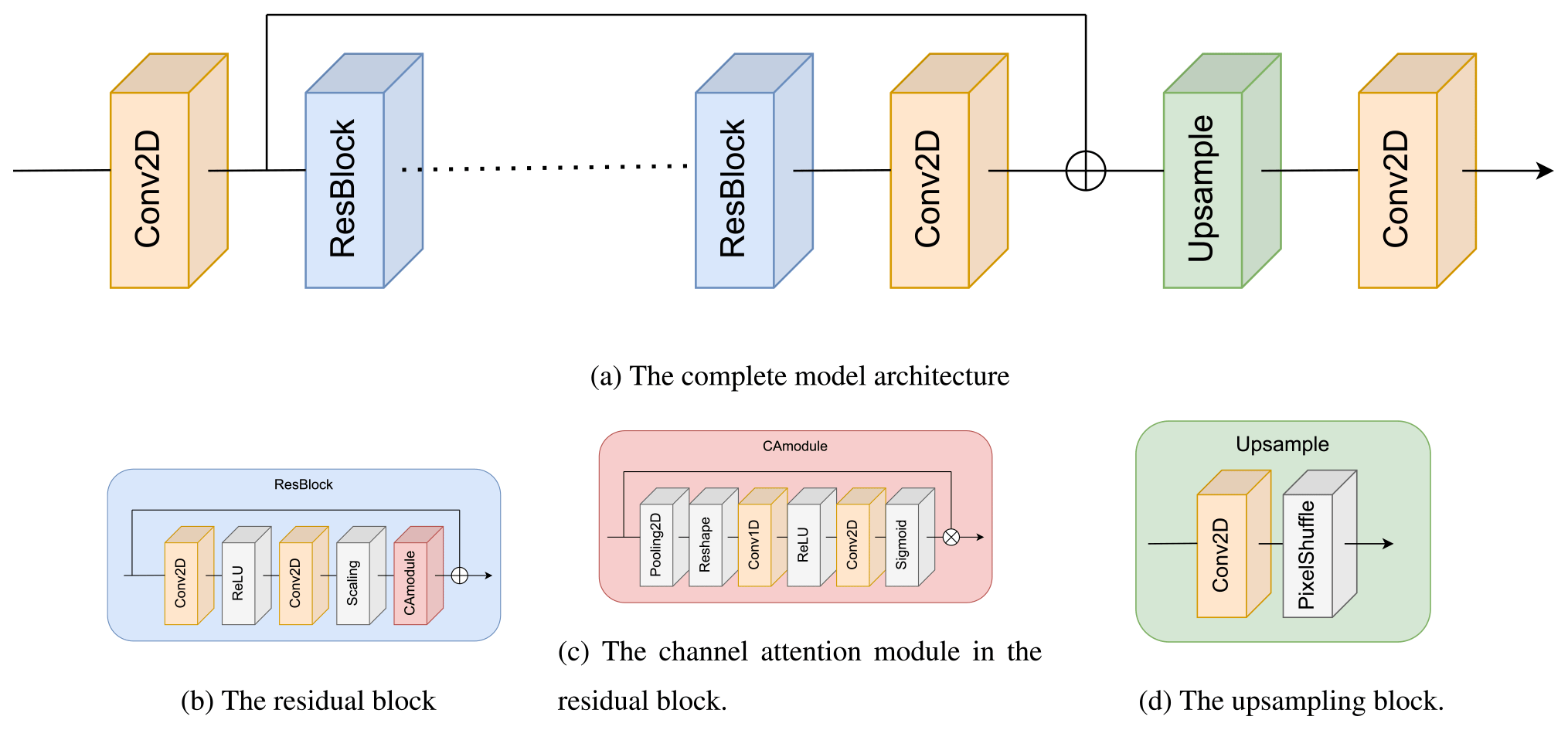
Figure 1 The overall layout of the neural network model (a) consists of an upsampling block (d) and residual blocks (b), which again contain a channel attention module (c). Here, ⊕ means adding the layers and ⊗ means multiplying them. The dotted line indicates that the residual block (b) is repeated multiple times.

2.2 Training data

To train our neural networks, we use data from the ECMWF ERA5 reanalysis (Hersbach et al., 2020). These global data are available hourly at a spatial resolution of 0.5^∘ × 0.5^∘ in latitude–longitude coordinates and with a total of 138 vertical levels (level indexes increase upward, contrary to ECMWF). We use a total of 296 h (from 1 to 12 January 2000) for training and test our model for 24 h in each season (on 15 January, 15 April, 15 July, 15 October 2000). Each hourly horizontal layer data point corresponds to a total of 138 layers, yielding a total of roughly 15 000 sample fields.

The low-resolution data are obtained from the high-resolution ERA5 data by simply sampling every first, second and fourth degree. Note that our approach of subsampling is driven by our goal to use the neural network as an interpolation algorithm, as required by kinematic trajectory calculations. From a dynamical point of view this is not the ideal approach, since averaged winds would give a dynamically more consistent representation of the flow. However, the goal here is not to provide the dynamically most consistent wind field but rather to obtain the best locally interpolated wind. Furthermore, averaging wind data would reduce the interpolation distance, since averaged winds would always be valid for locations very close to the location we want to interpolate to. For subsampling every first degree, for instance, we would need to interpolate only over one-quarter of a degree instead of half a degree, thus providing a much less rigorous test against the true wind. Finally, averaging winds is also not ideal for our purpose because the comparison of “true” winds and reconstructed winds would reflect the effect of both averaging and interpolating rather than interpolation alone.

In this work we focus solely on the spatial upscaling problem. The temporal upscaling problem will be considered elsewhere; see further discussions in the conclusions. We also only interpolate the horizontal wind components and interpolate only horizontally.

2.3 Neural network training

For each horizontal velocity component (u and v) we train a separate neural network to interpolate a field from degraded resolution data to double its resolution data. Then, (if necessary) the trained neural network is applied multiple times to interpolate 0.5^∘ resolution data. We train three sets of neural networks:

model1

to interpolate a field from degraded 1^∘ × 1^∘ resolution data to 0.5^∘ × 0.5^∘ resolution data;

model2

to interpolate a field from degraded 2^∘ × 2^∘ resolution data to 1^∘ × 1^∘ resolution data;

model4

to interpolate a field from degraded 4^∘ × 4^∘ resolution data to 2^∘ × 2^∘ resolution data.

For the evaluation we only use models 2 and 4 since those are the only models that allow us to apply to resolution not seen during training. Model 1 is trained using the highest-resolution data, and we cannot therefore use it to upscale to a higher resolution as we do not have the associated data for comparison.

We found that the wind field structure is different at higher and lower levels in the atmosphere, and it is thus beneficial to train separate neural networks for these two regions of the atmosphere. Thus, one neural network is trained for the lower atmospheric levels (up to level 50, approximately below the tropopause), and another one is trained for the higher levels (51 to 138). Each neural network is trained on the data of 294 hourly wind fields with 50 and 88 vertical levels. This results in 14 700 or 25 578 training samples, respectively.

The model was implemented using TensorFlow 2.8 and is made available in a repository (https://doi.org/10.5281/zenodo.7350568; Brecht et al., 2022). We trained the model on a dual NVIDIA RTX 8000 machine, with each training step taking approximately 100 ms for the u and v field. Total training took roughly 2.5 h for each field.

2.4 Interpolation error metrics

To evaluate the accuracy of the interpolation and trajectory simulation, we use the root mean square error (RMSE) and the structural similarity index measure (SSIM) as performance measures. The RMSE is defined as

$$\begin{array}{}\text{(1)}& {\text{RMSE}}_z=\sqrt{\stackrel{\mathrm{‾}}{(z_{\mathrm{interpolated}}-z_{\mathrm{reference}}{)}^{\mathrm{2}}}},\end{array}$$

where $z\in \mathit{\{}u,v\mathit{\}}$, with the bar denoting spatial averaging. The reference solution is given by the original 0.5^∘ × 0.5^∘ ERA5 data, assumed to represent the truth. The smaller the RMSE value, the better the interpolated results coincide with the original reference solution.

The SSIM is a measure of the perceived similarity of two images a, b and is defined as

$$\begin{array}{}\text{(2)}& \text{SSIM}(a,b)={\displaystyle \frac{(\mathrm{2}{\mathit{\mu }}_a{\mathit{\mu }}_b+C_{\mathrm{1}})(\mathrm{2}{\mathit{\sigma }}_{ab}+C_{\mathrm{2}})}{({\mathit{\mu }}_a^{\mathrm{2}}+{\mathit{\mu }}_b^{\mathrm{2}}+C_{\mathrm{1}})({\mathit{\sigma }}_a^{\mathrm{2}}+{\mathit{\sigma }}_b^{\mathrm{2}}+C_{\mathrm{2}})}},\end{array}$$

with μ_a and μ_b denoting the means of the two images a and b (computed with an 11×11 Gaussian filter with a width of 1.5), σ_a and σ_b denoting their standard deviations, and σ_ab being their co-variance. The constants C₁ and C₂ are defined as C₁=(K₁L)² and C₂=(K₂L)², with K₁=0.01 and K₂=0.03 and L=1. The closer the SSIM value is to 1, the more similar the two images are. See Wang et al. (2004) for further details. In the following, a=z_interpolated and b=z_reference, with each of them being interpreted as a gray-scale image.

2.5 Trajectory calculations

To test the impact of the neural-network-interpolated wind fields on trajectory calculations, we used the Lagrangian particle dispersion model FLEXPART (Pisso et al., 2019; Stohl et al., 2005). The calculations are conducted using a stripped down version 10.4 of FLEXPART. We switched off all turbulence and convection parameterizations and used FLEXPART as a simple trajectory model. Ideally, the neural network interpolation should be implemented directly in FLEXPART. However, as the neural network and FLEXPART run on different computing architectures (graphics vs. central processing unit), directly implementing the neural network interpolation into FLEXPART is beyond the scope of this exploratory study. Instead, we replaced the gridded ERA5 wind data with the gridded upsampled testing data produced by the neural network. Using gridded upsampled testing data does not make full use of the neural network capabilities, since the neural network only produces values at a fixed resolution of 0.5^∘ × 0.5^∘ latitude/longitude, while we still use linear interpolation of the wind data to the exact particle position when computing their trajectories. However, the neural network could in principle also determine the wind components almost exactly at the particle positions upon repeatedly using the trained SISR model to increase the resolution enough to obtain the wind values at the respective particle positions. FLEXPART also needs other data than the wind data, for which we use linear interpolation of the ERA5 data. For temporal and vertical interpolation, we also used linear interpolation, as is standard in FLEXPART.

We started multiple simulations with 10 million trajectories on a global regular grid with 138 vertical levels and traced the particles for 48 h. This simulation was repeated in each season for the following cases:

• the original ERA5 data at 0.5^∘ × 0.5^∘ resolution, serving as the ground-truth reference case;

• a data set for which the winds were interpolated from degraded 1^∘ × 1^∘ and from 2^∘ × 2^∘ resolution data, using linear interpolation as is standard in FLEXPART;

• a data set for which the winds were interpolated from degraded 1^∘ × 1^∘ (using the neural network model2 trained to interpolate 2^∘ × 2^∘ to 1^∘ × 1^∘) and from 2^∘ × 2^∘ resolution data (using the neural network model4 trained to interpolate 4^∘ × 4^∘ to 2^∘ × 2^∘) and then interpolated to the particle position using linear interpolation in FLEXPART.

2.6 Trajectory error metrics

As in previous studies (Kuo et al., 1985; Stohl et al., 1995), we compared the trajectory positions for trajectories calculated with the interpolated data to those calculated with the reference data set, using the absolute horizontal transport deviation (AHTD), defined as

$$\begin{array}{}\text{(3)}& \mathrm{AHTD}\left(\mathrm{t}\right)={\displaystyle \frac{\mathrm{1}}{N}}\sum _{n=\mathrm{1}}^{N}D\left[\right(X_n,Y_n,t),(x_n,y_n,t\left)\right],\end{array}$$

where N is the total number of trajectories and $D\left[\right(X_n,Y_n,t),(x_n,y_n,t\left)\right]$ is the great circle distance of trajectory points with longitude/latitude coordinates $(X_n,Y_n,t)$ for the reference trajectories and $(x_n,y_n,t)$ for the trajectories using interpolated winds at time t, for the trajectory pair n starting at the same point. AHTD values are evaluated hourly along the trajectories, up to 48 h.

3 Results

In this section, we first compare the neural-network-interpolated data to the linearly interpolated data. Then, we compare the accuracy of the trajectories computed with FLEXPART using the interpolated fields of the neural network to the linearly interpolated fields.

3.1 Interpolation

We investigate the self-similarity of the spatial scales by interpolating the fields multiple times using the same model trained to upscale the wind fields from lower resolutions. For the interpolation we use linear and neural network interpolation. First, we compare the fields which are interpolated from 1^∘ × 1^∘ to 0.5^∘ × 0.5^∘ resolution data. Then, we proceed with applying the neural network interpolation multiple times to generate an arbitrary resolution.

In Fig. 2 we show the interpolation results for three different neural networks and for the linear interpolation. Here, each neural network is used to interpolate each resolution, starting with the resolution the model is trained on. The interpolation error reduces with the resolution. We see that each neural network almost always has better metrics (i.e., lower RMSE and higher SSIM values) than the corresponding linear interpolation. This is true both for the resolution the neural network has been trained for as well as for higher resolutions.

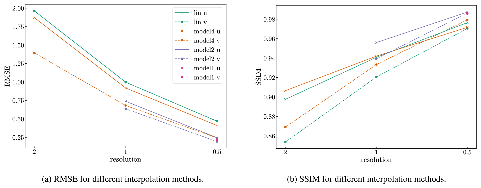
Figure 2 RMSE (a) and mean SSIM (b) of the validation data set (14 January 2000) for linear and neural network interpolation evaluated at different resolutions. Here, we do not interpolate the fields multiple times (as explained in Sect. 3.1.2) but rather once for each resolution starting from the resolution the model is trained on. The solid lines are computed for the u velocity and the dashed lines for the v velocity.

3.1.1 One-time upscaling

We first consider the neural network model2 (trained to interpolate 2^∘ × 2^∘ to 1^∘ × 1^∘ resolution data). For the evaluation we interpolate a field from degraded 1^∘ × 1^∘ resolution data to 0.5^∘ × 0.5^∘ resolution data. Note that we have trained the model separately for levels 0–50 and 51–137 (counting from the ground) and evaluate the correspondingly trained model.

In Fig. 3 we show the RMSE for the interpolated field for level 10 (corresponding approximately to an altitude of 245 m above ground level) and for one particular time (14 January at 10:00 UTC) as an example. Figure 3 also shows an enlarged region focusing on a cold front south of Australia, where we clearly see that the largest RMSE errors for both linear and neural network interpolation occur along the cold front. The winds in the boundary layer show a large wind shear between the southwesterly winds to the southeast of the cold front and the northwesterly winds to the northeast of the cold front. This causes large interpolation errors in the frontal zone. However, these large errors are substantially reduced by the neural network interpolation compared to the linear interpolation. This also means that the largest interpolation errors, in particular, are avoided by the neural network compared to the linear interpolation (see Fig. 4). This finding also holds for other conditions, as can be seen by the general error reduction in other regions on the globe (Fig. 3) and the smaller but still significant error reductions in cases with generally smaller interpolation errors (Fig. 4).

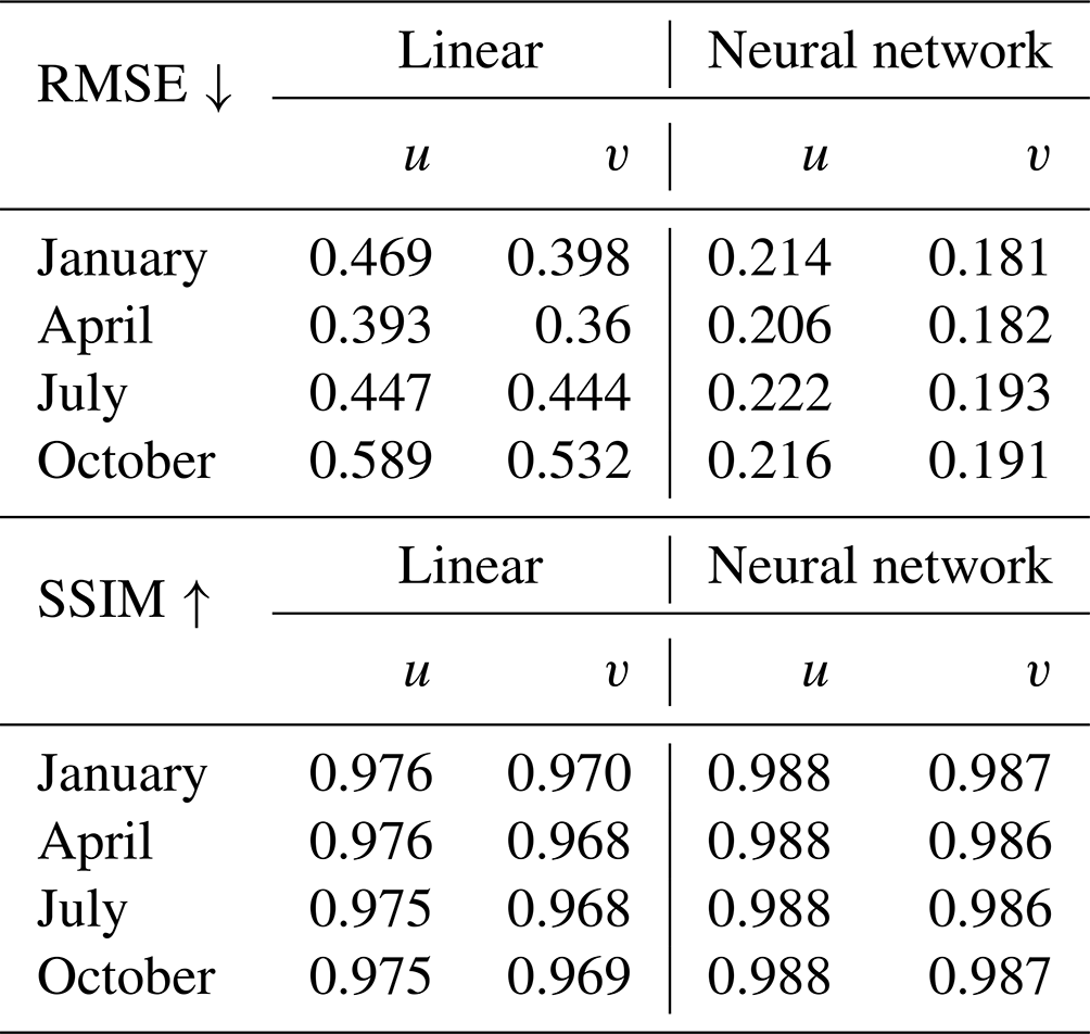
More example figures for the different months (January, April, July and October) can be found in the (Zenodo) repository. We note that the results are similar for the different months, as shown in Table 1, where we computed the RMSE and SSIM for a whole day in the months of January, April, July and October and for all levels. The neural network interpolation has less than half the RMSE of the linear interpolation and achieves a higher SSIM value.

We note that the interpolation time on our hardware for one field for a given level and time for the linear interpolation is about 10 times faster compared to the same interpolation using the neural network.

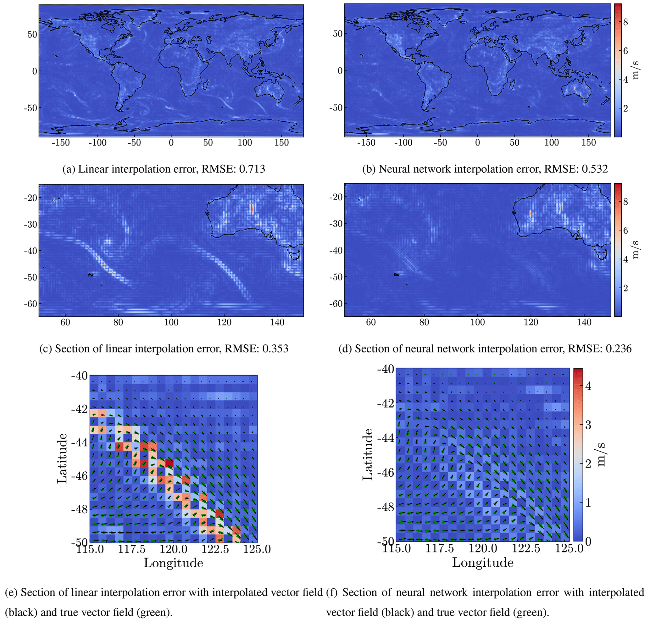
Figure 3 Differences between the $\mathbf{v}=(u,v)$ fields on the 14 January 2000 at 10:00 UTC for level 10 (around 245 m) and the truth ERA5 data, for linear interpolation (a, c, e) and for the interpolation by the model2 neural network (b, d, f). The data are interpolated from degraded 1^∘ × 1^∘ resolution data. The top row (a, b) shows the error on the globe and the panels below show an enlarged section of the top panels.

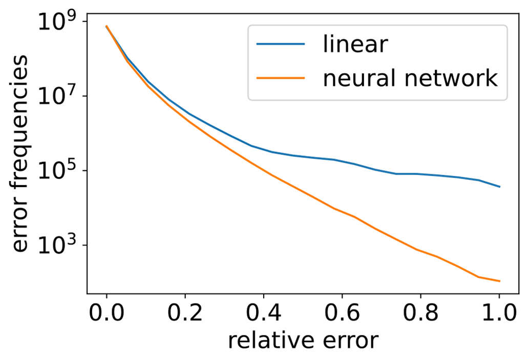
Figure 4 Comparison of the error frequencies for linear and neural network interpolation (model2) for 14 January 2000 (over all 137 vertical levels and over 24 h). Here, we normalized the error and split the error frequencies into 20 bins of different intensities.

Table 1 RMSE and mean SSIM of the validation data set for linear and neural network interpolation using model2. Considering the RMSE, the neural network interpolation is at least 49 % more accurate compared to the linear interpolation.

3.1.2 Multiple time upscaling

To demonstrate that the neural network can be used to interpolate a field to arbitrary resolution, we consider the neural network model4 ( trained to interpolate 4^∘ × 4^∘ to 2^∘ × 2^∘ resolution data). We apply the network to interpolate 2^∘ × 2^∘ to 1^∘ × 1^∘ and apply it another time to interpolate 1^∘ × 1^∘ to 0.5^∘ × 0.5^∘ resolution data. In Fig. 5 we evaluate the RMSE of an interpolated field in January at level 10 (around 245 m) and compare it to the RMSE of the linear interpolation.

For each method the RMSE is higher compared to the one-time upscaling, since we start with a lower resolution and less information. Nevertheless, the RMSE of the neural network interpolation is again lower compared to the linear interpolation, albeit the relative error reduction is smaller than with one-time upscaling (see Table 2). This also holds for other samples in different seasons which we omitted showing here. When evaluating the RMSE for a day in January, April, July and October for all levels (Table 2), we observe that the neural network interpolation is 19 % more accurate than the linear interpolation. Here, we are limited to the resolution of the reference data. Thus, we can only demonstrate the interpolation for two times. Coarser data do not have enough small scales represented, and it is therefore not meaningful to train the network on coarser data and upscale the data more times.

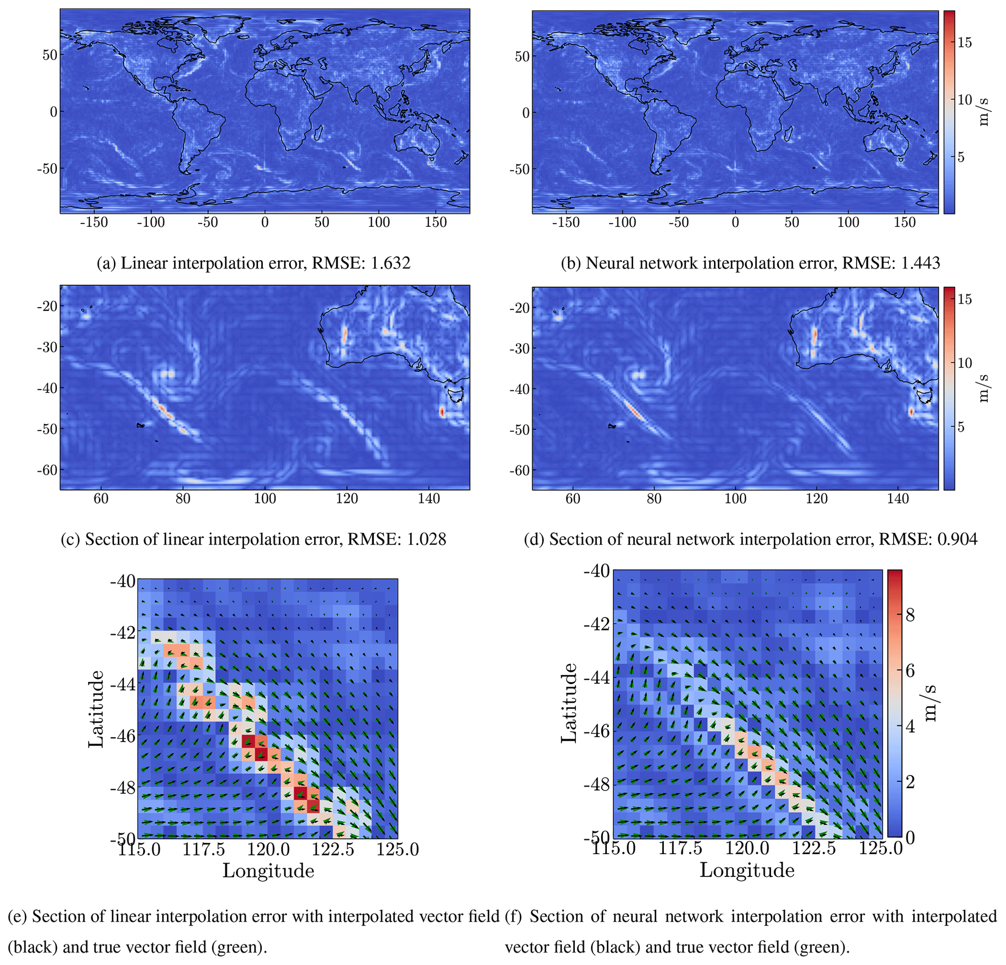
Figure 5 RMSE of $\mathbf{v}=(u,v)$ field at level 10 when compared to the truth ERA5 data. The date of the field is the 14 January 2000 at 10:00 UTC. Linear interpolation (a, c, e) and the interpolation by the neural network model4 (b, d, f). The data are interpolated from degraded 2^∘ × 2^∘ resolution data. The top row (a, b) shows the error on the globe and the panels below show an enlarged section of the top panels.

Table 2 RMSE and mean SSIM of the validation data set for linear and neural network interpolation, using model4. Considering the RMSE, the neural network interpolation is at least 19 % more accurate compared to the linear interpolation.

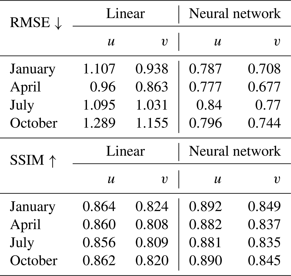
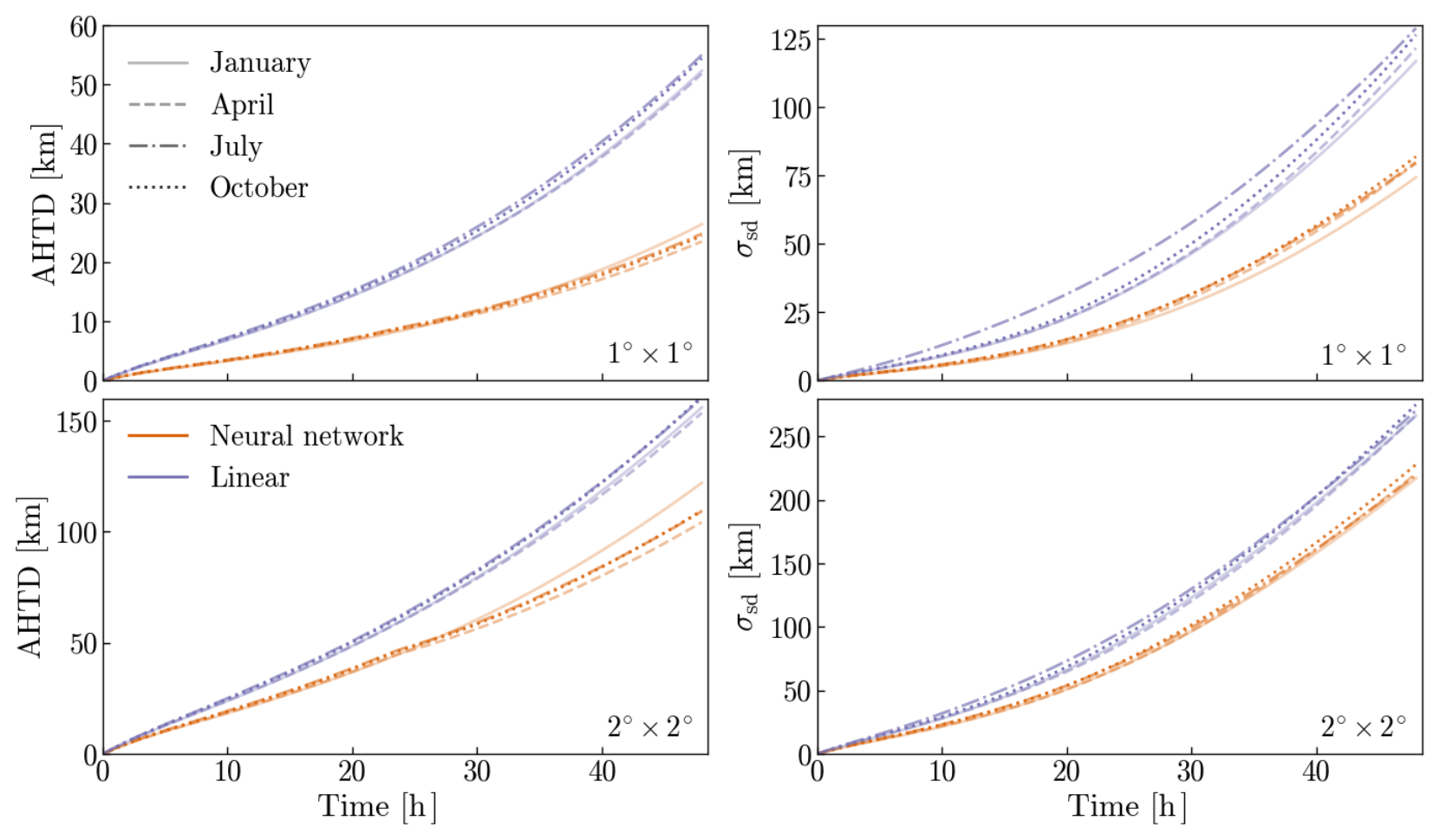
Figure 6 Absolute horizontal transport deviations (Eq. 3) and standard deviations of 10 million particles advanced with FLEXPART, using two different degraded resolution data (as described in Sect. 3.1) and two interpolation methods, as compared to the same particles advanced using the original full resolution data. The top panels show the results for the degraded 1^∘ × 1^∘ resolution data (neural network interpolation using model2), and the bottom panels those of the degraded 2^∘ × 2^∘ resolution data (neural network interpolation using model4). Orange lines show the AHTD (left panels) and standard deviation (right panels) of particles advanced using the neural network, and purple lines show these for the linearly interpolated data. Results for different seasons are shown with different line styles.

3.2 Trajectory accuracy

In the previous sections, we showed that our neural-network-interpolated wind velocity fields are more similar to the original 0.5^∘ × 0.5^∘ resolution data than their linearly interpolated equivalents. However, this does not necessarily mean that trajectories advanced using the neural-network-interpolated fields are more accurate. Trajectories are not always equally sensitive to wind interpolation errors, and it is therefore important to show that the individual trajectories that are advanced using neural-network-interpolated wind fields are indeed more similar to trajectories that are advanced using the original “ground-truth” wind fields.

Figure 6 shows that trajectories that are advanced using neural-network-interpolated wind fields are closer to trajectories that are advanced using the original ground-truth wind fields compared to trajectories using linearly interpolated wind fields. Here, we show the results of the horizontal transport deviation (Eq. 3) and standard deviations of particles advanced for 48 h, using FLEXPART, after being initially globally distributed. Both the average horizontal transport deviation from the original ground-truth trajectories as well as its standard deviation are smaller for the neural network than the linear interpolation. The absolute deviations after 48 h are on average ∼53.5 % (1^∘ × 1^∘ resolution) and ∼29.4 % (2^∘ × 2^∘ resolution) smaller for all seasons when using the neural network. Moreover, the standard deviation of the neural network is consistently smaller, no matter the season (on average ∼36.1 % and ∼17.9 % smaller for the 1^∘ × 1^∘ and 2^∘ × 2^∘ resolution, respectively). The improvement in the neural network over the linear interpolation is smaller with multiple-time upscaling from 2^∘ × 2^∘ resolution than with one-time upscaling from 1^∘ × 1^∘ resolution, since the latter has smaller wind interpolation errors (see Fig. 2). The reduced standard deviation we see in the neural-network-interpolated trajectories as compared to the linearly interpolated ones is likely a result of the lower frequency of extreme deviations found in the neural-network-interpolated wind fields as compared to the linearly interpolated ones (see Fig. 4). Thus, trajectories using the neural network interpolation are not only more accurate on average than trajectories using linear interpolation, but large trajectory errors are avoided more efficiently as well. This is important for avoiding misinterpretation when trajectories are used to interpret source–receptor relationships, e.g., for air pollutants or greenhouse gases.

We have also checked how well the quasi-conserved meteorological property of potential vorticity is conserved along the trajectories by computing absolute and relative transport conservation errors along trajectories in the stratosphere. We excluded particles affected by convection or boundary layer turbulence by selecting trajectories within the stratosphere that never traveled through space where the relative humidity exceeded 90 %. A full explanation of the method we used can be found in Stohl and Seibert (1998). The absolute and relative transport conservation errors in potential vorticity showed insignificant differences between the different trajectory data sets.

Note that we have not changed vertical and time interpolation of the winds and that we have not changed the interpolation of the vertical wind. Furthermore, we have not made full use of the neural network horizontal interpolation of the horizontal winds, as interpolation below 0.5^∘ × 0.5^∘ resolution was still done using linear interpolation. We therefore consider substantial further error reductions possible, if neural network interpolation both in space and time is fully implemented directly in the trajectory model. This way neural network interpolation could make semi-Lagrangian advection schemes much more accurate.

4 Conclusions

In this paper we have considered the problem of increasing the spatial resolution of meteorological fields using techniques of machine learning, namely using methods originally proposed for the problem of single-image super-resolution. Higher-resolution meteorological fields are relevant for a variety of meteorological and engineering applications, such as particle dispersion modeling, semi-Lagrangian advection schemes, down-scaling and weather nowcasting.

What sets the present work apart from a pure computer vision problem is that meteorological fields are characterized by self-similarity over a variety of spatiotemporal scales. This gives rise to the possibility of training a neural network to learn to increase the resolution from a downsampled meteorological field to the original native resolution of that field, and then to repeatedly apply the same model to further increase the resolution of that field beyond the native resolution. We have shown in this paper that this is indeed possible. Wind interpolation errors are at least 49 % and 19 % smaller than errors using linear interpolation, with one-time upscaling and with multiple-time upscaling, respectively. Here, we note that the multiple-time upscaling has a lower improvement than the one-time upscaling because we use different neural networks based on the available resolution. This means that the neural network trained on lower-resolution data has less information and is less accurate than the neural network trained on the higher-resolution data. We have also shown that corresponding absolute horizontal transport deviations for trajectories calculated using these wind fields are 52 % (from degraded 1^∘ × 1^∘ resolution data) and 24 % (from degraded 2^∘ × 2^∘ resolution data) smaller than with winds based on linear interpolation. This is a substantial reduction, given that we have not changed vertical and time interpolation and that we have not at all changed the interpolation of the vertical wind. Furthermore, we have not even made full use of the neural network interpolation, as interpolation below 0.5^∘ × 0.5^∘ resolution was still done using linear interpolation.

While in the present work we have exclusively focused on the spatial interpolation improvement problem, similar techniques as presented here are applicable to the temporal interpolation case as well. Here, the problem can be interpreted as increasing the frame rate in a given video clip, with the native resolution given by the temporal resolution as made available by numerical weather prediction centers. We are presently working on this problem as well, and the results will be presented in future work. Subsequently, spatial and temporal resolution improvements can be combined to provide a seamless way to increase the overall resolution of meteorological fields for a variety of spatiotemporal interpolation problems.

Lastly, we should like to stress that meteorological fields are quite different from conventional photographic images as typically considered for super-resolution tasks. Namely, meteorological fields follow largely a well-defined system of partial differential equations, which we have not considered when increasing the spatial resolution of the given data sets. This means that potentially important meteorological constraints such as energy, mass and potential vorticity conservation may be violated by obtained upscaled data sets, as is also the case for other interpolation methods. Incorporating these meteorological constraints would be critical if these fields were used in conjunction with numerical solvers, and correspondingly the proposed methodology would have to be modified to account for these constraints. This will constitute an important area of future research, with a potential avenue being provided through so-called physics-informed neural networks. See, e.g., the studies by Raissi et al. (2019) and Bihlo and Popovych (2022) for an application of this methodology to solving the shallow-water equations on the sphere. Physics-informed neural networks allow one to take into account both data and the differential equations underlying these data, which would enable one to train a neural-network-based interpolation method that is also consistent with the governing equations of hydro-thermodynamics. Including consistency with these differential equations will be another potential avenue of research in the near future.