the Creative Commons Attribution 4.0 License.
the Creative Commons Attribution 4.0 License.
 | 23 Sep 2022
Uncertainty and sensitivity analysis for probabilistic weather and climate-risk modelling: an implementation in CLIMADA v.3.1.0
Chahan M. Kropf
Alessio Ciullo
Laura Otth
Simona Meiler
Arun Rana
Emanuel Schmid
Jamie W. McCaughey
David N. Bresch
Modelling the risk of natural hazards for society, ecosystems, and the economy is subject to strong uncertainties, even more so in the context of a changing climate, evolving societies, growing economies, and declining ecosystems. Here, we present a new feature of the climate-risk modelling platform CLIMADA (CLIMate ADAptation), which allows us to carry out global uncertainty and sensitivity analysis. CLIMADA underpins the Economics of Climate Adaptation (ECA) methodology which provides decision-makers with a fact base to understand the impact of weather and climate on their economies, communities, and ecosystems, including the appraisal of bespoke adaptation options today and in future. We apply the new feature to an ECA analysis of risk from tropical cyclone storm surge to people in Vietnam to showcase the comprehensive treatment of uncertainty and sensitivity of the model outputs, such as the spatial distribution of risk exceedance probabilities or the benefits of different adaptation options. We argue that broader application of uncertainty and sensitivity analysis will enhance transparency and intercomparison of studies among climate-risk modellers and help focus future research. For decision-makers and other users of climate-risk modelling, uncertainty and sensitivity analysis has the potential to lead to better-informed decisions on climate adaptation. Beyond provision of uncertainty quantification, the presented approach does contextualize risk assessment and options appraisal, and might be used to inform the development of storylines and climate adaptation narratives.
- Article
(4626 KB) - Full-text XML
- BibTeX
- EndNote


Societal impacts from natural disasters have steadily increased over the last decades (IFRC, 2020), and they are expected to follow the same path under climatic, socio-economic, and ecological changes in the coming decades (IPCC, 2021). This creates the need for better preparedness and adaptation towards such events, and raises a demand for risk assessments and appraisals of adaptation options at local, national, and global levels. Typically, such studies are carried out through the use of computer models – which will be referred to as climate-risk models in this paper – that allow us to estimate the socio-economic and ecological impact1 of various natural hazards such as tropical cyclones, wildfires, heat waves, droughts, coastal, fluvial, or pluvial flooding.
The specific setup of climate-risk models depends on the hazard under consideration, the location of interest, and the goal of the study. However, such models often share a similar structure given by three sub-models, usually referred to as hazard, exposure, and vulnerability. These constitute the input variables of climate-risk models and represent the main drivers of climate risk as defined by the Intergovernmental Panel on Climate Change (IPCC) (IPCC, 2014a). Hazard is a model of the physical forcing at each location of interest; exposure is a model of the spatial distribution of the exposed elements such as people, buildings, infrastructures, and ecosystems; and vulnerability is characterized by a uni- or multivariate impact function describing the impact of the considered hazard on the given exposed elements. By combining hazard, exposure, and vulnerability, the socio-economic impact of natural hazards can be assessed. In so doing, one can also carry out an appraisal of adaptation options by comparing the current and future risk reduction capacity of adaptation options with expected implementation costs.
In practice, the quantification of risk with climate-risk models is particularly challenging as it involves dealing with the absence of robust verification data (Matott et al., 2009; Pianosi et al., 2016; Wagener et al., 2022) when setting up the hazard, exposure, and vulnerability sub-models, as well as dealing with large uncertainties in the input parameters and the model structure itself (Knüsel, 2020). For example, in hazard modelling, many authors have shown large uncertainties affecting the computation of flood maps through hydraulic modelling (Merwade et al., 2008; Dottori et al., 2013); similarly, alternative models have been proposed for modelling tracks and intensities of tropical cyclones (Emanuel, 2017; Bloemendaal et al., 2020). For exposure, notable uncertainties are associated with the quality of the data being used; their resolution; and, since proxy data are often used (Ceola et al., 2014; Eberenz et al., 2020), their fitness for purpose. The vulnerability module also introduces significant uncertainties, because data needed to calibrate impact function curves are often very scarce and scattered (Wagenaar et al., 2016). In addition, uncertainties affecting exposure, hazard, and vulnerability are exacerbated by the unknowns in climatic, economical, social, and ecological projections. Furthermore, modelling adaptation options is a process that is particularly strongly affected by normative uncertainties (Knüsel et al., 2020). For example, the choice of the discount rate, which affects the effectiveness of a given option, raises intergenerational justice issues (Doorn, 2015; Moeller, 2016; Mayer et al., 2017). Finally, the choice of output metrics, the performance measures, and the very formulation of the risk management problem also underlie value-laden choices (Kasprzyk et al., 2013; Ciullo et al., 2020), as they dictate what actors and what actors' interests are included in the risk assessment and appraisal of adaptation options (Knüsel et al., 2020; Otth, 2021; Otth et al., 2022).
Uncertainty and sensitivity analyses are among the established methods proposed by the scientific literature to quantitatively treat uncertainties in model simulation (Saltelli et al., 2008). While for both methods an analytical treatment is preferable (Norton, 2015), it is often not possible. Therefore, numerical Monte Carlo or quasi-Monte Carlo schemes (Lemieux, 2009; Leobacher and Pillichshammer, 2014) are applied, which require repeated model runs using different values for the uncertain input parameters. Uncertainty analysis is then the study of the distribution of outputs obtained when the uncertain input parameters are sampled from plausible uncertainty ranges. Ideally, these plausible ranges should be defined based on background knowledge related to these parameters (Beven et al., 2018b). Sensitivity analysis in turn assesses the respective contributions of the input parameters to the total output variability, and often builds upon uncertainty analysis. It allows us to test the robustness of the model, single out the input uncertainties most responsible for the output uncertainty, and improve understanding about the model's structure and input–output relationships (Pianosi et al., 2016). Arguably, conducting uncertainty and sensitivity analyses should be part of any modelling exercise as it reveals its fitness for purpose and limitations (Saltelli et al., 2019). Nevertheless, uncertainty and sensitivity analyses are still lacking in many published modelling studies (Beven et al., 2018a; Saltelli et al., 2019). In this context, climate-risk assessment studies are no exception. Although there are examples in the scientific literature of applications of uncertainty and sensitivity analyses to the full (de Moel et al., 2012; Koks et al., 2015) or partial (Hall et al., 2005; Savage et al., 2016) climate-risk modelling chains, these techniques (Douglas-Smith et al., 2020) are neither common practice, nor applied in a systematic fashion. This may strongly undermine the quality of the risk assessment and appraisal of adaptation options, and may lead to poor decisions (Beven et al., 2018a).
In order to fill this gap and facilitate the widespread adoption and application of uncertainty and sensitivity analyses in climate-risk models, this paper introduces and showcases a new feature of the probabilistic climate-risk assessment and modelling platform CLIMADA (CLIMate ADAptation) (Aznar-Siguan and Bresch, 2019; Bresch and Aznar-Siguan, 2021; Kropf et al., 2022a), which seamlessly integrates the SALib – Sensitivity Analysis Library in Python package (Herman and Usher, 2017) into the overall CLIMADA modelling framework, and thus supports all sampling and sensitivity index algorithms implemented therein. The new feature allows conducting uncertainty and sensitivity analyses for any CLIMADA climate-risk assessment and appraisal of adaptation options with little additional effort, and in a user-friendly manner. Here, we describe the UNcertainty and SEnsitity QUAntification (unsequa) module in detail and demonstrate it's use of a previously published case study on the impact of tropical cyclones in Vietnam (Rana et al., 2022).
The paper is structured as follows: Sect. 2 will introduce the CLIMADA modelling platform and describe how uncertainty and sensitivity analyses are integrated therein; Sect. 3 demonstrates the use of uncertainty and sensitivity analyses by revisiting a case study on the impact of tropical cyclone in Vietnam; Sect. 4 discusses results and provides an outlook.
2.1 Brief introduction to CLIMADA
To our knowledge, CLIMADA is the first global platform for probabilistic multi-hazard risk modelling and options appraisal to seamlessly include uncertainty and sensitivity analyses in its workflow, as described in this section. CLIMADA is written in Python 3 (Van Rossum and Drake, 2009); it is fully open source and open access (Kropf et al., 2022a). It implements a probabilistic global multi-hazard natural-disaster impact model based on the three sub-modules, i.e. hazard, exposure, and vulnerability. It can be used to assess the risk of natural hazards and to perform appraisal of adaptation options by comparing the averted impact (benefit) thanks to adaptation measures of any kind (from grey to green infrastructure, behavioural, etc.) with their implementation costs (Aznar-Siguan and Bresch, 2019; Bresch and Aznar-Siguan, 2021).
The hazard is modelled as a probabilistic set of events, each one a map of intensity at geographical locations, and with an associated probability of occurrence. For example, the intensity can be expressed in terms of flood depth in metres, maximum wind speed in metres per second, or heat wave duration in days, and the probability as a frequency per year. The exposure is modelled as values distributed on a geographical grid. For instance, the number of animal species, the value of assets in dollars, or the number of people living in a given area. The vulnerability is modelled for each exposure type by an impact function, which is a function of hazard intensity (for details, see Aznar-Siguan and Bresch, 2019). For example, this could be a sigmoid function with 0 % of affected people below 0.2 m flood depth, and 90 % of affected people above 1 m flood depth. The adaptation measures are modelled as modification of the impact function, exposure, or hazard. For example, a new regional plan can incite people to relocate to less flood-prone areas, hence resulting in a modified exposure (cf. Aznar-Siguan and Bresch, 2019; Bresch and Aznar-Siguan, 2021).
The risk of a single event is defined as its impact multiplied by its probability of occurrence. The impact is obtained by multiplying the value of the impact function at a given hazard intensity with the exposure value at a given location. The total risk over time is obtained from the impact matrix, which entails the impact of each hazard event at each exposure location, and the hazard frequency vector. The benefits of adaptation measures are obtained as the change in total risk. Both the total risk and the benefits can thus be computed for today and in the future, following climate-change scenarios and socio-economic development pathways (cf. Aznar-Siguan and Bresch, 2019; Bresch and Aznar-Siguan, 2021).
With CLIMADA, risk is assessed in a globally consistent fashion, from city to continental scale, for historical data or future projections, considering various adaptation options, including future projections for the climate, socio-economic growth, or vulnerability changes.
2.2 Uncertainty and sensitivity quantification (unsequa) module overview
The general workflow of the new uncertainty and sensitivity quantification module unsequa, illustrated in Fig. 1, follows a Monte Carlo logic (Hammersley, 1960) and implements similar steps as generic uncertainty and sensitivity analyses schemes (Pianosi et al., 2016; Saltelli et al., 2019). It consists of the following steps:
-
Input variables and input parameters definition. The probability distributions of the uncertain input parameters (random variables) are defined. They characterize the input variables – hazard, exposure, and impact function for risk assessment and, additionally, adaptation measures for appraisal of adaptation options – of the climate-risk model CLIMADA.
-
Samples generation. Samples of the input parameter values are drawn according to their respective uncertainty–probability distribution.
-
Model output computation. The CLIMADA engine is used to compute all relevant model outputs for each of the samples for risk assessment (risk metrics) and/or appraisal adaptation options (benefit and cost metrics).
-
Uncertainty visualization and statistics. The distribution of model outputs obtained in the previous step are analysed and visualized.
-
Sensitivity indices computation. Sensitivity indices for each input parameter are computed for each of the model output metric distributions.
-
Sensitivity visualization and statistics. The various sensitivity indices are analysed and visualized.
We remark that the third and fourth steps typically constitute the core elements of the uncertainty analysis, and the fifth and sixth steps the core elements of the sensitivity analysis. In Sect. 2.3, we describe each one of the steps in more detail. Detailed documentation on how to use the unsequa module is available at https://climada-python.readthedocs.io/ (last access: 30 August 2022).
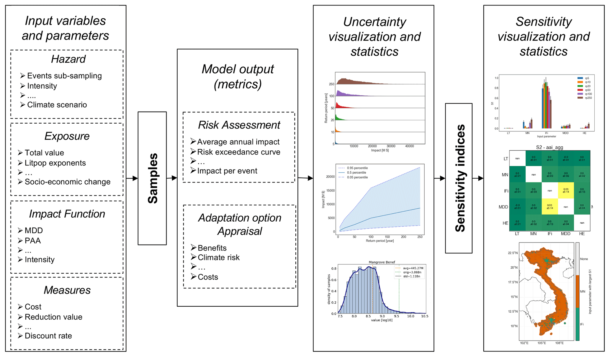
Figure 1The workflow for uncertainty and sensitivity analyses with the unsequa module in CLIMADA consists of six steps (from left to right). (1) Define the input variables (hazard, exposure, impact function, adaptation measure) and their uncertainty input parameters (e.g. hazard intensity, total exposure value, impact function intensity, measures cost). (2) Generate the input parameter samples. (3) Compute the model output metrics of interest for risk assessment and appraisal of adaptation options for each sample using the CLIMADA engine. (4) Analyse the obtained uncertainty distributions with statistical tools and provide a set of visualizations. (5) Compute the sensitivity indices for each input parameter and each output metric. (6) Analyse the sensitivity indices by means of statistical methods and provide different visualizations.
2.3 Detailed workflow of unsequa module
2.3.1 Input variables and parameters
The CLIMADA engine integrates the input variables exposure (E), hazard (H), and impact function (F) for risk assessment. For the appraisal of adaptation options, the exposure and impact function are combined with the adaptation measure (M) in a container input variable called entity (T). Note that further input variables might be added in future versions of CLIMADA. Each of these input variables comes with any number of uncertainty input parameters α, distributed according to an independent probability distribution pα. An input variable can have any number of uncertainty input parameters, and there is no restriction on the type of probability distributions (uniform, Gaussian, skewed, heavy-tailed, discrete, etc.). In the current implementation, any distribution from the Scipy.stats Python module (Virtanen et al., 2020) is accepted. The input parameters can define any variation or perturbation of the input variables (e.g. initial conditions, boundary conditions, forcing inputs, resolutions, normative choices, etc.). 2 Note that the choice of the variation and the associated range and distribution can substantially affect the results of uncertainty and sensitivity analyses (Paleari and Confalonieri, 2016). Ideally, this modelling choice should be made based on solid background knowledge. However, the latter is often lacking or highly uncertain; in such cases, we encourage users to explore how the results may vary with alternate distributions and choices of input parameters. It is thus about not only deriving definitive quantitative values describing the deviation of the climate-risk model's output from the “real” value, but also assessing the robustness, sensitivity, and plausibility of the model output under clearly defined assumptions.
Overall, the user must define one method for each of the uncertain input variables X, which returns the input variable's value for each valid value of the associated uncertain input parameters . The latter are univariate random variables distributed according to . In order to support the user, a series of helper methods are implemented in the unsequa module (cf. Appendix B). This general problem formulation allows for the parametrization of generic uncertainty, with broadly speaking two types of approaches: (1) an input variable is directly perturbed with statistical methods; or (2) the underlying model used to generate the input variable is fed with the uncertain parameters. Note that each input variable is independent, and thus either approach can be used for different input variables for the same study (cf. the illustration case study in Sect. 3.1).
As one example, suppose we are modelling the impact of heat waves on people in Switzerland. As exposure layer, we might use gridded population data based on the total population estimate from the UN World population prospect (United Nations, Department of Economic and Social Affairs, Population Division, 2019), reported to be ts=8 655 000 in 2020. Assuming an estimation error of ±5 %, the input variable E has one uncertain input parameter t with a uniform distribution pt between [0.95ts,1.05ts]. As hazard, we might consider the heat waves of the past 40 years as measured by the Swiss Meteorological institute. Disregarding measurement uncertainties, one could decide to model this without uncertainty. Finally, the impact function might be represented by a sigmoid function calibrated on past events which yields uncertainty for the slope s and the asymptotic value a. The slope's uncertainty could be a multiplicative factor s drawn from a truncated Gaussian distribution ps with mean 1, standard deviation 0.2, and the truncation of negative values, while the asymptotic value could be given by a which follows a uniform distribution pa between [0.8,1].
As another example, we are interested in the risk of floodplain flooding for gridded physical assets in the Congo basin. The flood hazard is generated from a floodplain modelling information system (FMIS) with uncertainty parameters describing the uncertainty in the geospatial data, the temporal data, the model parameters (Mannings), and the hydraulic structure, such as shown in Merwade et al. (2008). These input parameters are used directly as uncertainty input parameters for the unsequa model, with a wrapper method returning a CLIMADA hazard object produced from the FMIS flood inundation map. In addition, the exposures are obtained by interpolating and downscaling satellite images to a resolution r (Eberenz et al., 2020). The sensitivity and robustness to the resolution choice is modelled by pre-computing exposures at resolutions . The uncertainty parameter is then r, with a uniform choice distribution between the pre-computed values. Finally, we consider all assets to be described by a single impact function, which is derived from three different case studies found in literature. The impact function's uncertainty is defined as a uniform choice-distributed parameter corresponding to the selection of one of the three impact functions.
Defining the appropriate input variable uncertainty and identifying the relevant input parameters for a given case study are not trivial tasks. In general, only a small subset of all possible parameters can be investigated Dottori et al. (2013), Pianosi et al. (2016). In order to identify the relevant parameters and defining the input variables' uncertainty accordingly, one can for instance use an assumption map (Knüsel et al., 2020), as presented for CLIMADA in Otth (2021), and Otth et al. (2022). Another general strategy is to proceed iteratively: first a broad sensitivity analysis is used to identify the most likely important uncertainties, followed by a more detailed uncertainty and sensitivity analyses for full quantification.
2.3.2 Samples
In general, there are two basic approaches regarding how samples can be drawn. In the local “one-at-a-time” approach, the input parameters are varied one after another, keeping all the others constant (Pianosi et al., 2016). Local methods are conceptually simpler, but capture neither interactions between input parameters nor non-linearities (Douglas-Smith et al., 2020). By contrast, in global methods, the input parameters are sampled from the full space at once (Matott et al., 2009). This allows for a more comprehensive depiction of model uncertainty by accounting for the interactions among the input parameters. Saltelli et al. (2019) even argue that uncertainty and sensitivity analyses should always be based on global methods for models with non-linearities such as CLIMADA.
Hence, the basic premise of the unsequa module is to use a global sampling algorithm based on (quasi-) Monte Carlo sequences (Lemieux, 2009; Leobacher and Pillichshammer, 2014) to generate a set of N samples of the input parameters. Here, one sample refers to one value for each of the input parameters. Following the heat wave example described in Sect. 2.3.1, one would create N global samples with . One sample thus corresponds to a set of three numbers in this case. Choosing the correct number of samples is a notoriously difficult task (Iooss and Lemaître, 2015; Sarrazin et al., 2016). One generic approach is to start with a sample size that one can afford to generate reasonably efficiently (e.g. N∼100D), and then check the confidence intervals of the estimated sensitivity indices (cf. Sect. 2.3.5). If relative values of the estimated indices are too ambiguous to draw key conclusions due to the overlap of confidence intervals, one should either generate more samples, or use a more frugal method (e.g. reduce the number of input parameters D) (Sarrazin et al., 2016).
CLIMADA imports the (quasi-) Monte Carlo sampling algorithms from the SALib Python package (Herman and Usher, 2017). Thus, all sampling algorithms from this package are directly available to the user within the unsequa module. These algorithms are all implemented for a uniform distribution over [0,1] at least. In order to accommodate any input parameter distributions, the unsequa module uses the percent-point function (ppf) of the target probability density distribution (cf. Appendix A).
2.3.3 Model output: risk assessment and appraisal of adaptation options
For each sample of the input parameters, the model output metrics are computed using the CLIMADA engine, e.g. for the risk assessment, the impact matrix In for each sample xn. Following the heat wave example from the previous section, for each sample of the input parameters, the algorithm first sets the input variables , and . Second, the corresponding impact matrix In is computed for each sample independently, following the algorithm described in Aznar-Siguan and Bresch (2019). All CLIMADA risk output metrics such as the average annual impact, the exceedance frequency curve, or the largest event are then derived from the matrix In and the hazard frequency defined in H(n).
Similarly, for the appraisal adaptation options, each sample is assigned with the corresponding input variables. The CLIMADA engine is then used to compute the impact matrix for each sample n, each adaptation measure m, and each year y following the algorithm described in Bresch and Aznar-Siguan (2021). All CLIMADA benefit and cost metrics such as the total future risk, the adaptation-measure benefits, the risk transfer options, and costs are derived from the impact matrix , the adaptation measure Mm(n,y), the exposure E(n,y) and the hazard H(n,y). Note that in practice, the input variables for the exposure, impact function, and adaptation measure are combined into one input variable called entity T(n,y), which also includes information about optional discount rates and risk transfer options.
We remark that no direct evaluation of the convergence of this quasi-Monte Carlo scheme is provided in the unsequa module, as it is not generally available for all the possible sampling algorithms available through the SALib package. Instead, the sensitivity analysis algorithms, to be described in Sect. 2.3.5 below, provide confidence intervals. In SALib, confidence intervals relate to the bounds which cover 95 % of the possible sensitivity index value, estimated through bootstrap resampling. These can be used as a proxy to assess the convergence of the uncertainty analysis. If the intervals are large and overlapping, the result is likely not robust and the number of samples should be increased.
In all of the uncertainty and sensitivity analyses, computing the model outputs is usually the most expensive step computationally. For convenience, an estimation of the total computation time for a given run is thus provided in the unsequa module. Experiments showed that the computation time scales approximately linearly with the number of samples N; it is also proportional to the time for a single impact computation. The latter is mostly defined by the size of the exposure (i.e. depends on the resolution, size of the considered geographical area, etc.) and the size of the hazard (i.e. depends on the number of events, the centroid's resolution, etc.). In case the input variables are generated using an external model (e.g. a hydrological flood model for the hazard), the computation time is also proportional to the external model run time. For complex models, this can be prohibitively long. In such cases, one can pre-compute the samples for the given input variable, thus trading CPU time for memory (cf. Litpop example in Sect. 3.2.1, and the helper methods in Appendix B). The number of samples N in turn scales with the dimension D (i.e. the number of input parameters), depending on the chosen sampling method. For the default unsequa module, Sobol′ method, the scaling is O(D). In addition, for the appraisal of adaption options, the risk computation is repeated for each of the Nm adaptation measures. This results in a total computation-time scaling of O(D) for the risk assessment, and O(D⋅Nm) for the appraisal of adaptation options. Thus, for large number of input parameters, and/or long single impact computation times, and/or large numbers of adaptation measures, the computation time might become intractable. In this case, one could consider using surrogate models (Sudret, 2008; Marelli and Sudret, 2014), a feature that might be added to future iterations of the unsequa module.
2.3.4 Uncertainty visualization and statistics
The output metrics values for each sample are characterized and visualized. To this effect, various plotting methods have been implemented as shown in Sect. 3.2.5 and 3.3.5. For instance, it is possible to visualize the full distributions or compute any statistical value for each model output metric. The key objective is to obtain an understanding of the uncertainties in the model outputs beyond the mean value and standard deviation.
2.3.5 Sensitivity indices
The sensitivity index Sα(o) is a number that subsumes the sensitivity of a model output metric o to the uncertainty of input parameter α (Pianosi et al., 2016). Since CLIMADA is a non-linear model, only global sensitivity indices are suitable (Saltelli and Annoni, 2010). To derive such global sensitivity indices, several algorithms are made available through the SALib Python package (Herman and Usher, 2017), including variance-based (ANOVA) (Sobol′, 2001), elementary effects (Morris, 1991), derivative-based (Sobol′ and Kucherenko, 2009), FAST (Cukier et al., 1973), and more (Saltelli et al., 2008). Importantly, each method requires a specific sampling sequence to compute the model output distribution and results in distinct sensitivity indices. These distinct indices will typically agree on the general findings (e.g. what input parameter has the largest sensitivity), but might differ in the details as they correspond to fundamentally different quantities (e.g. derivatives against variances). The recommended pairing of the sampling sequence and sensitivity index method is described in the SALib documentation, and simple save-guard checks have been implemented in the unsequa module. Note that it is technically valid to use different sampling algorithms for the uncertainty and for the sensitivity analyses. For example, one can first use sampling algorithm A to perform an uncertainty analysis, i.e. steps from Sect. 2.3.1–2.3.4. Then, one can use another sampling algorithm B as required for the chosen sensitivity index algorithm to perform the sensitivity analysis, i.e. steps from Sect. 2.3.1–2.3.3 and 2.3.5, 2.3.6. However, in practice, since generating samples is often the computational-time bottleneck, it is more convenient to use the same methods so that the same samples can be used for both analyses (Borgonovo et al., 2017).
For typical case studies using CLIMADA, Sobol′ indices are generally well-suited for both uncertainty and sensitivity analyses. For sampling the algorithm, the use of the Sobol′ quasi-Monte Carlo sequence (Sobol′, 2001) is required, which provides good rates of convergence when the number of input parameters is lower than ∼25 (Lemieux, 2009). Sobol′ indices are obtained as the ratio of the marginal variances to the total variance of the output metric. In particular, the algorithm implemented in the SALib package allows us to estimate the first-order, total-order, and second-order indices (Saltelli, 2002). First-order indices measure the direct contribution to the output variance from individual input parameters. Total-order indices measure the overall contribution from an input parameter considering its direct effect and its interactions with all the other input parameters. Second-order indices describe the sensitivity from all pairs of input parameters. In addition, the 95th percentile confidence interval is provided for all indices. This allows us to estimate whether the number N of chosen samples was sufficient for both the uncertainty and sensitivity analysis. Note that in general, the rate of convergence depends non-trivially on the number of input parameters, the probability distributions of the input parameters, the type of sensitivity index, and the sampling algorithm (Herman and Usher, 2017).
2.3.6 Sensitivity visualization and statistics
The last step consists of analysing and visualizing the obtained sensitivity indices. To this effect, a series of visualization plots are provided, such as bar plots or sensitivity maps for first-order indices, and correlation matrices for second-order indices, as shown in Sect. 3.2.5 and 3.3.6. This step shows which input parameters' uncertainty is the driver of the uncertainty of each individual module output metric. This is useful to support model calibration and verification, to prioritize efforts for uncertainty reduction, and to inform robust decision-making.
In the following discussion, we revisit a case study on tropical cyclone storm surges in Vietnam (Rana et al., 2022), and perform an uncertainty and sensitivity analysis on the risk assessment and appraisal of adaptation options to illustrate the use of the CLIMADA-unsequa module.
3.1 Case study description
We only consider the parts of the climate-risk study by Rana et al. (2022) that modelled the impact of Vietnam's tropical cyclone storm surges in terms of the number of affected people. The authors assessed the risk under present and future climate conditions, and performed an appraisal of adaptation options by computing the benefits and costs for three physical adaptation measures – mangroves, sea dykes, and gabions. A more detailed recount of the case study is provided in Appendix C.
Below, we showcase uncertainty and sensitivity analyses for the risk of storm surges in terms of affected people under present (2020) climate conditions in Sect. 3.2, and for the benefit and cost of the adaptation measure in 2050, considering the climate change Representative Concentration Pathways (RCP) 8.5 (IPCC, 2014a) in Sect. 3.3. The goal is to illustrate the use of the unsequa module, rather than to present a comprehensive uncertainty and sensitivity analysis for the case study. Thus, some of the uncertainties are defined in a stylized fashion by defining plausible distributions. A more in-depth analysis would require the use of, e.g. an argument-based framework (Otth, 2021; Otth et al., 2022; Knüsel et al., 2020), and would be beyond the scope of this paper.
For simplicity, hereafter (Rana et al., 2022) will be referred to as the original case study.
3.2 Risk assessment
The six steps of the uncertainty and sensitivity analyses (cf. Fig. 1) are described in detail in the following sections for the risk assessment of storm surges in Vietnam under present (2020) climate in terms of the number of affected people.
3.2.1 Input variables and parameters
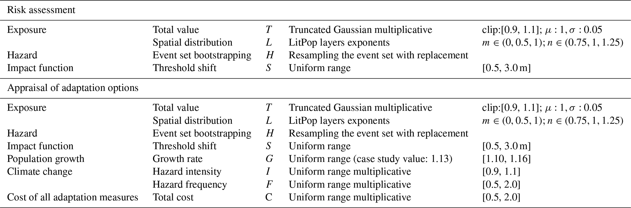
We identified four main quantifiable uncertainty parameters which are summarized in the upper row of Table 1. As we remarked above, the choice of the distribution of input parameters can substantially influence the results of the uncertainty and sensitivity analyses; it should thus ideally be based on background knowledge. The distributions chosen here are plausible, yet stylized, and should not be considered as general references for other case studies.
For the exposure, the total population is assumed to be subject to random sampling errors that are well captured by a normal distribution, and a maximum error of ±10 % is assumed. Thus, the total population is scaled by a multiplicative input parameter T, distributed as a truncated Gaussian distribution, with clipping values 0.9,1.1, mean value μ=1, and variance σ=0.05. For the population distribution, the original case study used the Gridded Population of the World (GPW) dataset (CIESIN, 2018), which is available down to admin-3 levels. To account for uncertainties arising from the finite resolution, we use the CLIMADA's LitPop module (Eberenz et al., 2020) to enhance the data with nightlight satellite imagery from the Black Marble annual composite of the VIIRS day–night band (Grayscale) at 15 arcsec resolution from the NASA Earth Observatory (Hillger et al., 2014), a common technique used to rescale population densities to higher resolutions (Anderson et al., 2014; Berger, 2020). In LitPop, the nightlight and population layers are raised to an exponent m and n, respectively, before the disaggregation. Here, we vary the value of m and n as a description of the uncertainty in the population distribution. In the original case study, m is set to 0 and n to 1. We consider the addition of the nightlight layer with , and vary the population layer with . The corresponding distributions are shown in Fig. D1. A higher value of n emphasizes highly populated areas, a lower value the sparsely populated areas. The corresponding input parameter L represents all pairs of (m,n).
For the hazard, we apply a bootstrapping technique, i.e. uniform resampling of the event set with replacement to account for the uncertainties of sample estimates. Since the default Sobol′ global sampling algorithm requires repeated application of the same value of any given input parameter, here we define H as the parameter that labels a configuration of the resampled events. Errors from the hazard modelling (cf. Appendix C) are not further considered here. A more detailed study might want to explore further uncertainty sources, such as the wind-field model, the hazard resolution, or the random event set generation algorithm.
Finally, for the impact function, we consider the uncertainty in the threshold of the original step function that was used to estimate the number of people “affected” (widely defined) by storm surges. In the original case study, the threshold was 1 m, with 0 % affected people below, and 100 % affected people above. We consider a threshold shift S between 0.5 and 3 m. This extends a range examined in a study of human displacement due to river flooding (there from 0.5–2 m) (Kam et al., 2021), in order to extensively explore the uncertainty related to resolution of the population and topography. This distribution does not examine a specific impact, but rather how the total number of people affected varies based on different thresholds used to define “affected”. The resulting range of the impact function is shown in Fig. D2.
Table 1Summary of the input parameter distributions. The input parameters T, L, and G characterize the uncertainty in the exposure (people), H, I, and F in the hazard (storm surge), S in the impact function (vulnerability), and C in the adaptation measures (mangroves, sea dykes, gabions). The parameters T, L, H, and S are needed for risk assessment (cf. Sect. 3.2.1), and the parameters T, L, H, S, G, I, F, and C are needed for adaptation options appraisal (cf. Sect. 3.3.1).
3.2.2 Samples
We use the default Sobol′ sampling algorithm (Sobol′, 2001; Saltelli and Annoni, 2010) to generate a total of 10 240 samples as shown in Fig. D3.
3.2.3 Model output
For each of the samples n, the full impact matrix In is obtained and saved for later use. Furthermore, from the impact matrix, we compute several risk metrics for each sample: the average annual impact aggregated over all exposure points, the aggregated risk at returns periods of 5, 10, 20, 50, 100, and 250 years, the impact at each exposure point, as well as the aggregated impact for each event (for details cf. Aznar-Siguan and Bresch, 2019).
3.2.4 Uncertainty visualization and statistics
In the following discussion, we concentrate on the analysis of the full uncertainty distribution of various risk metrics. For convenience, the original case study value, the uncertainty mean value, and standard deviation are also reported. However, as we shall see below, focusing only on these numbers would provide a limited picture.
The full uncertainty distribution for each of the return periods, as well as the exceedance frequency curve are shown in Fig. 2. First, we remark that the exceedance frequency curve of the original case study, shown in Fig. 2b, is close to the median percentile, while the upper and lower 95th percentiles of the uncertainty are roughly +40 % and −60 % compared to the median, respectively. Second, the distribution of uncertainty for each return period separately, shown in Fig. 2a, is in fact bimodal, particularly for shorter return periods. The original case study values for the lower return periods are all among the higher mode. Third, the distribution of the average annual impact aggregated over all exposure points, shown in Fig. 2c, is also bimodal, with the original case study lying in the mode with larger impacts. The mean number of affected people is 1.42 M with a variance of ±1.03 M, which is compatible with, but lower than the original case study value of 1.94 M.
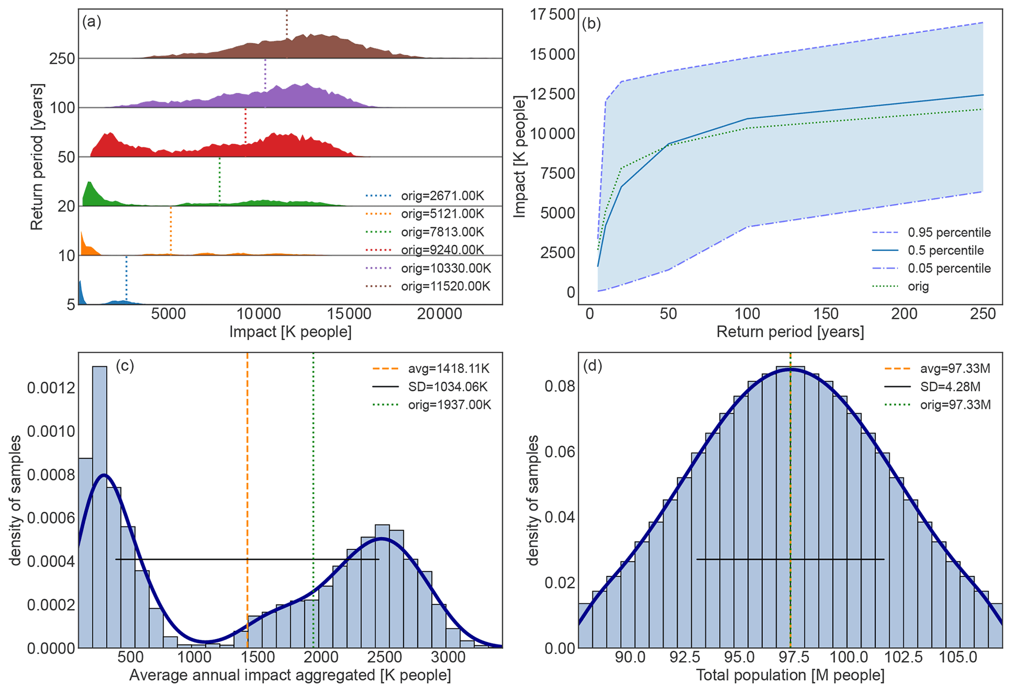
Figure 2Uncertainty distribution for storm surge risk in terms of affected people in Vietnam for present climate conditions (2020). (a) Full range of the uncertainty distribution of impacted people for each return period ( years) and value in the original study (vertical dotted lines). (b) Impact exceedance frequency curve shown for the original case study results (dotted green line), the median percentile (solid blue line), 5th percentile (dash-dotted blue line), and 95th percentile (dashed blue line). (c) Distribution of annual average impact aggregated over all exposure points (histogram bars) and (d) distribution of the uncertainty of the total population, i.e. the total exposure value, (histogram bars). Panels (c) and (d) both include the average value (vertical dashed orange line), original case study result (vertical dotted green line), standard deviation (horizontal solid black line), and kernel density estimation fit to guide the eye (solid dark-blue line). The impacts are expressed in thousands (K) or millions (M) of affected people.
The bimodal form of the impact uncertainty distribution is interesting, as one could rather expect statistical white or coloured noise (e.g. Gaussian or power-law distributions). As a consistency proof that this is not due to a computational setup error, we verified that the distribution of the total asset value, shown in Fig. 2d, aligns with the parametrization of the exposure uncertainty (cf. Table 1). For a better understanding of the obtained uncertainty distributions, particularly understanding the bimodality, let us continue with the sensitivity analysis.
3.2.5 Sensitivity indices
Ideally, we should choose the sensitivity method best suited for the data at hand. In our case, the uncertainty distribution is strongly asymmetric (cf. Fig. 2), thus a density-based approach would be best (Pianosi and Wagener, 2015; Borgonovo, 2007; Plischke et al., 2013). However, this would require generating a new set of samples, and for the purpose of this demonstration, we used the unsequa default variance-based Sobol′ method. Note that despite the questionable use of variances to characterize sensitivity for multi-modal uncertainty distributions, the derived indices prove useful to better understand the results from the case study at hand.
We thus computed the total-order and the second-order Sobol′ indices (Sobol′, 2001) for all the input parameters T, L, H, and S. We obtained the sensitivity indices for all the risk metrics shown in Fig. 2: average annual impact aggregated (aai_agg), impact for return periods of 5, 10, 20, 50, 100, and 250 years (rp5, rp10, rp20, rp50, rp100, rp250), and additionally for the average annual impact at each exposure point.
3.2.6 Sensitivity visualization and statistics
As shown in Fig. 3a, for the average annual impact aggregated, the largest total-order sensitivity index is for the impact function threshold shift with STS(aai_agg)≈0.95. This indicates that the uncertainty in the impact function threshold shift S is the main driver of the uncertainty. Thus, to understand the bi-modality of the uncertainty distribution (cf. Fig. 2c), we have to better understand the relation between S and the model output. Note that there are no strong interactions between the input parameter uncertainties as all second-order sensitivity indices S2≈0 (cf. Fig. D6). Thus, it is reasonable to assume that the bi-modality of the distribution comes directly from S and not from correlation with other input parameters. We further remark that the 95th percentile confidence intervals of the sensitivity indices (indicated with vertical black bars in Fig. 3) are much smaller than the difference between the sensitivity indices. We thus conclude that the number of samples was sufficient for a reasonable convergence of the uncertainty and sensitivity sampling algorithm.

Figure 3Total order Sobol′ sensitivity indices (ST) for storm surge risk for people in Vietnam in the present climate conditions (2020). Panel (a) shows results for the average annual impact aggregated over all exposure points (aai_agg); (b) represents the map of the largest sensitivity index at each exposure point. The category “None” refers to areas with vanishing risk. (c) Sensitivity results for risk estimate over return periods (rp) years. The input parameters (cf. Table 1) are T: total population, L: population distribution, S: impact function threshold shift, and H: hazard events bootstrapping. The vertical black bars in (a) and (b) indicate the 95th percentile confidence interval.
A further analysis of the average annual impact aggregated value in function of the impact function threshold shift S reveals a discontinuity at a value of Sd∼1.85 m as shown in Fig. D5a. Hence, the bimodality of the uncertainty distributions (cf. Fig. 2) is indeed due to the uncertainty input parameter S of the impact function, but it does not explain the root cause. Further understanding is obtained from studying the storm surge footprint used in the original case study. Plotting the storm surge intensity of all events at each location with values ordered from smallest to largest, we find a discontinuity and plateau around 1.85 m, as shown in Fig. D5b. This is the value corresponding to the threshold shift at which the average annual impact is discontinuous. Thus, the bimodality of the uncertainty distributions, while caused by uncertainty in the impact function, is rooted in the modelling of the storm surge hazard footprints. Further research beyond the scope of this paper would be needed to understand whether this value of 1.85 m has a physical origin (e.g. landscape features or protection standards), or is due to a modelling artefact. However, despite the discontinuity, the patterns are as expected: an impact function with a step at 0.5 m results in many more people being classified as affected than when the step is at 3 m (in the latter case, only particularly large storm surges would result in people being affected). For planning purposes, the lower end of this impact function shift is most relevant – even 0.5 m depth of a storm surge can be dangerous for people – so the higher mode of the distribution in Fig. 2 is most relevant.
Finally, the largest sensitivity index for the average annual impact at each exposure point is reported on a map in Fig. 3b. In the highly populated regions around Ho Chi Minh city (South Vietnam) and Haiphong (North Vietnam), the largest index is S in accordance with the sensitivity of the average annual impact aggregated over all of Vietnam. However, in less densely populated areas, such as the larger Mekong delta (South Vietnam), the outcome is more sensitivity to the population distribution L. Furthermore, while for shorter return periods, the largest total-order sensitivity index is the impact function threshold shift STS, for longer return periods the sensitivity to the population distribution STL becomes larger as shown in Fig. 3c. This might be because stronger events with large return periods consistently have larger intensities than the maximum threshold shift of 3 m. Together, these results hint to potentially hidden high-impact events in unexpected areas (e.g. a large storm surge in the less densely populated southern tip of Vietnam could affect a large number of people).
3.3 Appraisal of adaptation options
We focus on the appraisal of the three adaptation measures, i.e. mangroves, sea dykes, and gabions, to reduce the number of people affected by storm surges assuming the high-emission climate-change scenario RCP8.5. We consider the time period 2020–2050 as in the original case study.
3.3.1 Input variables and parameters
We identified four additional quantifiable uncertainty input parameters for the appraisal of adaptation options compared to the risk-assessment study (cf. Sect. 3.2.1) that are summarized in the bottom row of Table 1. For the exposure, the growth rate of the population from 2020 to 2050 was estimated at 13 % in the original case study based on data from the United Nations (United Nations, Department of Economic and Social Affairs, Population Division, 2019). Here, we assume a growth rate G uniformly sampled between 10 % and 16 %. For the hazard, the original case study used the parameters from Knutson et al. (2015) to scale the intensity and frequency of the events, considering the climate-change scenario RCP8.5 from 2020 to 2050 (see Appendix C for more details). This method is subject to large uncertainties (see e.g. Knüsel et al., 2020) and we thus scale the intensity and frequency with parameters I and F, uniformly sampled from [0.9,1.1] and [0.5,2], respectively. Finally, the cost of the adaptation measures is assumed to vary by a multiplicative factor C, sampled uniformly between [0.5,2].
3.3.2 Samples
For the sampling, we use the default Sobol′ sampling algorithm to generate a total of N=18 432 samples. Owing to the larger amount of input parameters, the total number of samples is larger than for the risk assessment (cf. Sect. 3.2.2). The drawn samples are shown in Fig. D4.
3.3.3 Model output
For each of the samples, we obtained the cumulative output metrics over the whole time period 2020–2050. In particular, we obtained the total risk without adaptation measures, the benefits (averted risk) for each adaptation measure, and the cost of each adaptation measure (for details see Bresch and Aznar-Siguan, 2021). One can then compare the cost–benefit ratios, i.e. the cost in dollars per reduced number of affected people, for each of the adaptation measures including model uncertainties.
3.3.4 Uncertainty visualization and statistics
The uncertainty for the cumulative, total average annual risk from storm surges aggregated over all exposure points is shown in Fig. 4d. The distribution is bimodal, which can be traced back to the storm surge model as explained in Sect. 3.2.3. The original case study value is located in the larger mode, similar to the average annual risk in 2020 as discussed in Sect. 3.2.3. This bimodality translates to the uncertainty in the benefit (total averted risk) for the adaptation measure sea dykes, Fig. 4b, but not to the adaptation measures mangroves and gabions, Fig. 4a and c. Rather, the latter show a heavy-tail uncertainty distribution. Furthermore, the uncertainty analysis of the ratio of the cost to the benefits for each adaptation measure indicates that, contrary to the original case study, the sea dykes might in fact be the least (instead of the most) cost-efficient adaptation measure (see Fig. D7a–c). Note that expressing the cost-efficiency of an adaptation measure in terms of a reduced number of affected people for each invested dollar presents ethical challenges as will be discussed in more detail in Sect. 4.

Figure 4Uncertainty distribution (histogram bars) for benefits (averted risk) from the adaptation measures: (a) mangroves, (b) sea dykes, (c) gabions, and (d) the total risk without adaptation measures. Benefits and total risk are cumulative over the time period 2020–2050 for the climate-change scenario RCP8.5. Vertical dotted green lines indicate the case study value, vertical dashed orange lines show the average benefit over the uncertainty distribution, the horizontal solid black line shows the standard deviation, and the solid dark-blue line indicates the kernel density estimation fit to guide the eye. The benefits and total risk are expressed in millions (M) of affected people.
3.3.5 Sensitivity indices
We use the same method as for the risk assessment to compute the total-order ST and the second-order S2 Sobol′ indices (Sobol′, 2001) for all the input parameters (cf. Table 1). We obtain the sensitivity indices for all the metrics shown in Figs. 4 and D7, i.e. the total risk as well as the benefits and cost–benefit ratios for all adaptation measures.
3.3.6 Sensitivity visualization and statistics
The total risk without adaptation measure is most sensitive to the impact function threshold shift S with STS(total risk)≈0.85 as shown in Fig. 5b. In addition, the sensitivity to the storm surge frequency changes STF(total risk)≈0.18 is significantly larger than the sensitivity to the intensity changes SI(total risk)≈0.02. This could be a consequence of the choice to use a step function to model the vulnerability.
The uncertainty of the benefits for all adaptation measures are most sensitive to the impact function threshold shift, with , and as shown in Fig. 5a. This is consistent with the sensitivity of the risk in 2020 (cf. Fig. 3). Furthermore, there is some sensitivity to the people distribution L, and to the uncertainty in the climate-change input parameters I and F. Note, however, that , i.e. the uncertainty of the benefits from the adaptation measure sea dykes is not sensitive to the hazard intensity uncertainty, while it is for both mangroves and gabions. This could be because sea dykes are parameterized to reduce the storm surge level by 2 m, which is above the Sd=1.85 m identified in Sect. 3.2.3 as critical for the surge modelling, while gabions and mangroves are parameterized to provide a reduction of 0.5 m which is below (cf. Appendix C and Rana et al., 2022). Thus, a change in the hazard frequency and the population distribution patterns will result in a stronger variation of the benefits for sea dykes because fewer, but stronger events contribute to the remaining risk each year.
Note that the 95th percentile confidence intervals of the sensitivity indices (indicated with vertical black bars in Fig. 5) are much smaller than the difference between the sensitivity indices. We thus conclude that the number of samples was sufficient for a reasonable convergence of the uncertainty and sensitivity sampling algorithm.
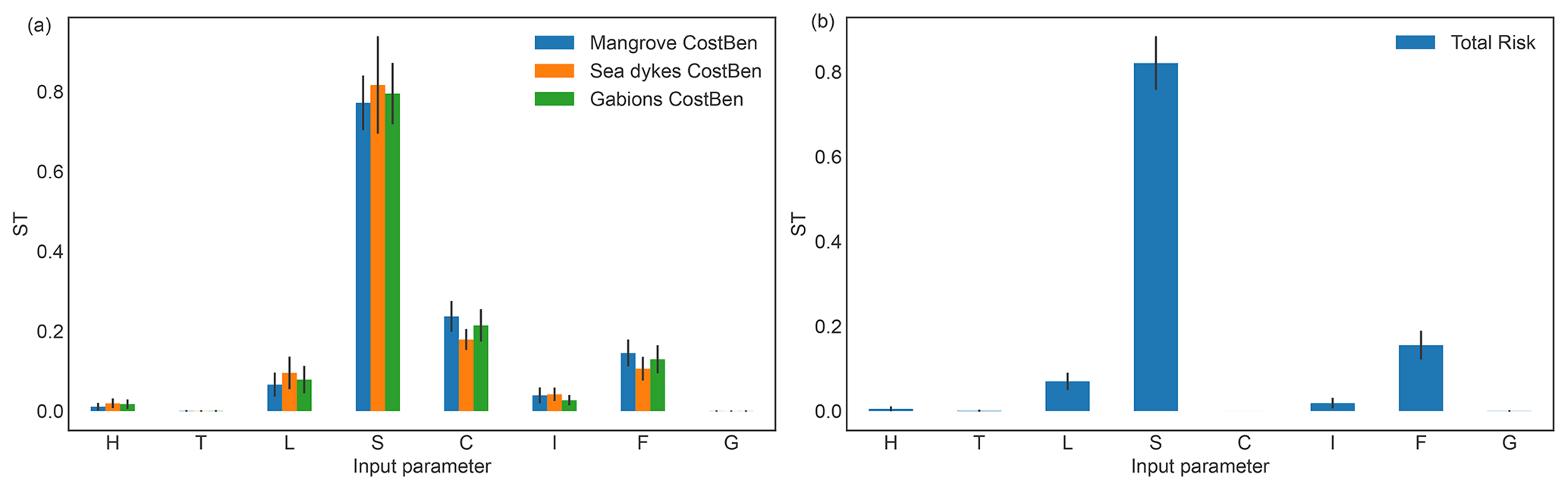
Figure 5Total-order Sobol′ sensitivity indices (ST) for the uncertainty of (a) storm surge adaptation options benefits for mangroves, sea dykes, and gabions and of (b) the total risk without adaptation measures, for the time period 2020–2050 under the climate-change scenario RCP8.5. The input parameters (cf. Table 1) are H: hazard events bootstrapping, T: total population, L: population distribution, S: impact function intensity threshold shift, C: cost of adaptation options, I: hazard intensity change, F: hazard frequency change, and G: population growth. The vertical solid black bars indicate the 95th percentile confidence interval.
3.4 Summary of the case study
The original case study intended to serve as a blueprint for future analyses of other world regions with limited data availability, and thus focused on the application of established research tools to provide insights into natural hazard risks and potential benefits of adaptation options (Rana et al., 2022). In view of limited observational data for impacts from tropical cyclones, the results of the study should have been subject to considerable uncertainty. The need for uncertainty and sensitivity analyses was identified within the original study, but deemed out of scope. This was partly due to the absence of a comprehensive and easily applicable scheme, now resolved with the uncertainty and sensitivity quantification (unsequa) module presented here. In addition, a full-fledged uncertainty and sensitivity analysis leads to a large number of additional data to process. Indeed, the results shown in this section considered only a small subset of the original case study, which, among others, also considered the impact of tropical cyclone wind gusts, and the impact of wind and surge on physical assets in dollars. Nevertheless, the benefits of an uncertainty and sensitivity analysis are manifest. On the one hand, it provides a much more comprehensive picture on risk from storm surges and the benefits of identified adaptation measures. On the other hand, it allows us to identify the main shortcomings of the model, which is needed to focus modelling improvement efforts and to understand the limitations of the obtained results. Even when used in the context of studies such as ECA, which are bound by time and money, this is useful to improve the confidence in, and transparency of the outcomes, and allows model improvements from study to study. For instance, in this section, it was conclusively shown that in order to improve the impact modelling, one should focus on the storm surge model, among other aspects. Furthermore, the analysis showed that urban and rural regions might not be equally well-represented by the model.
In this paper, we described the unsequa module for uncertainty and sensitivity analyses recently added to the climate-risk model CLIMADA. We highlighted its ease of use with an application to a previous case study assessing risks from tropical storm surges to people in Vietnam and appraising local adaptation options. We showed that only providing percentile information without the full distributions can be misleading, and that uncertainty analysis without sensitivity analysis does not provide a thorough picture of uncertainty (Saltelli and Annoni, 2010). The example showed the vital role played by uncertainty and sensitivity analyses in not only producing better and more transparent modelling data, but also providing a more comprehensive context to quantitative results in order to better support robust decision-making (Wilby and Dessai, 2010). This expansion of the CLIMADA platform allows for risk assessment and options appraisal, including quantification of uncertainties in a modular form and occasionally bespoke fashion (Hinkel and Bisaro, 2016), yet with the high re-usability of common functionalities to foster usage in interdisciplinary studies (Souvignet et al., 2016) and international collaboration. Further, the presented approach can be used to inform the development of storylines (Shepherd et al., 2018; Ciullo et al., 2021) and climate adaptation narratives (Krauß and Bremer, 2020).
The illustrative case study in this paper was run on a computing cluster. However, many potential users will not have access to such computational resources. Nonetheless, meaningful uncertainty and sensitivity analyses can be conducted only on a single computer, for instance by reducing resolution, sample size, or the number of uncertainty input parameters. For example, the illustrative case study in the paper could be run reasonably on a typical laptop by reducing the resolution to 150 arcsec. By doing so, it is not possible to explore all possible nuances, but one can still get a big-picture view of where key areas of uncertainty and sensitivity may lie.
While we showed that quantitative uncertainty and sensitivity are significant steps to improve the information value of climate-risk models, we stress that not all uncertainties can be described with the shown method (see e.g. Appendix D for a discussion on event uncertainty). Indeed, only the uncertainty of those input parameters that are varied can be quantified, and even for these input parameters, defining the probability distribution is subject to strong uncertainties, often being based only on educated guesses. Yet, the choice of probability distribution can have a strong impact on the resulting model output distribution and sensitivity (Paleari and Confalonieri, 2016; Otth, 2021; Otth et al., 2022). In addition, it is often not evident how to perturb the input variables, since one does not always have access to the underlying generating model, and it is otherwise difficult to define physically consistent statistical perturbations of geospatial data. Moreover, there is a large part of climate-risk models' uncertainty that is not even quantifiable in principle (Beven et al., 2018b; Knüsel et al., 2020). When building a climate-risk model, a number of things must be specified, such as the model type, the algorithmic structure, the input data, the resolution, the calibration and validation data, etc. These choices are often not made based on solid knowledge (Knüsel, 2020). One particular type of uncertainty that modellers are less familiar with is normative uncertainties; these arise from value-driven modelling choices (Bradley and Drechsler, 2014; Bradley and Steele, 2015) that are particularly relevant when the climate-risk analysis is carried out to support decisions and options appraisal. Normative uncertainties are rarely identified in common modelling practice (Bradley and Drechsler, 2014; Bradley and Steele, 2015; Moeller, 2016; Mayer et al., 2017). In most cases, these uncertainties can hardly be quantified and, therefore, they need to be addressed via methods such as argument analysis (Knüsel et al., 2020), the NUSAP methodology (Funtowicz and Ravetz, 1990), or sensitivity auditing (Saltelli et al., 2013). In some other cases, e.g. the decision regarding the value of a discount rate, normative uncertainties can be quantified, and quantitative analyses can highlight the effects of varying modelling choices on the decision outcomes. A complementary study to this paper proposes a methodological framework for a broader assessment of uncertainties for decision processes with CLIMADA as the climate-risk model, including both conceptual and quantitative approaches (Otth, 2021; Otth et al., 2022).
If a climate-risk modeller conducts uncertainty and sensitivity analyses, either by using the CLIMADA module published here, or by implementing a similar analysis in another modelling framework, the next question is: what should be done with the results? We suggest two main areas that could benefit from such analyses. First, within the field, the more that uncertainty and sensitivity analyses become standard practice, the more these analyses will enhance transparency of studies among climate-risk modellers. This can help to focus related research on areas that can provide better understanding of the parameters, or on modelling choices that are most influential on model outputs. Second, for decision-makers and other users of climate-risk modelling, uncertainty and sensitivity analyses have the potential to lead to better-informed decisions on climate adaptation. Several methods exist for inclusion into quantitative decision-making analysis (Hyde, 2006). Certainly, the numerical and graphical outputs of the module published here, or outputs from similar analyses, are far too technical to directly hand over as is to decision-makers and other users (unless the user is a risk analyst already versed in uncertainty and sensitivity analyses). Rather, the results of uncertainty and sensitivity analyses can inform discussions between climate-risk modellers and decision-makers about how best to refine and interpret model results. It is especially important to reflect additionally on uncertainties that lie outside the model and thus were not analysed in the quantitative uncertainty and sensitivity analyses (Otth, 2021; Otth et al., 2022). Further research and reflective practice can focus on how to most effectively achieve this.
In future iterations, uncertainty analysis in CLIMADA could for instance be extended with the addition of surrogate models to reduce the computational costs and allow for the testing of a larger number of input parameter with a larger number of samples for models at higher resolution. Overall, we hope that the simplicity of use of the presented unsequa module will motivate modellers to include uncertainty and sensitivity analyses as natural parts of climate-risk modelling. Finally, we caution that numbers even with elaborate error bars and distributions can give a false sense of accuracy (Hinkel and Bisaro, 2016; Katzav et al., 2021) and that modellers should remember to reflect on the wider, non-quantifiable uncertainties, unknowns, and normative choices of their models.
CLIMADA imports the quasi-Monte Carlo sampling algorithms from the SALib Python package (Herman and Usher, 2017). Thus, all sampling algorithms from this package are directly available to the user within the new module. These algorithms are all at least implemented for uniform distribution pu over [0,1]. In order to accommodate any input parameter distributions, the CLIMADA module uses the percent-point function (ppf) Q (also called inverse cumulative distribution, percentiles or quantile function) of the target probability density distribution. For example, in order to obtain a sample of N Gaussian-distributed pG values, one first samples values uniformly from [0,1], and then applies the ppf of the Gaussian distribution QG,
In the unsequa module, a number of helper methods exist to parameterize a few common uncertainty parameter distributions for the main input variables: exposure, impact functions, hazard, and measures, as summarized in Table B1. These helper methods are for the convenience of the users only. Any other uncertainty parameter can be introduced, and any other uncertainty parameter distributions (discrete, continuous, multi-dimensional, etc.) can be defined by the user if needed. For instance, the user could write a wrapper function around an existing dynamical hazard model which outputs a CLIMADA hazard object, and define the input factors of said dynamical model as uncertainty parameters.
For risk assessment, the impact at an exposure location x for an event ϵ is defined (Aznar-Siguan and Bresch, 2019) as
where fx is the impact function for the exposure at location x, and are the hazard intensity and fraction of event ϵ at the location closest to x, and v(x) is the value of the exposure at location x. Considering all locations and all events defines the impact matrix I. All further risk metrics, such as the average annual impact aggregated, are derived from I and the annual frequency νϵ of each hazard event. The helper methods are defined to describe generic uncertainties on the input variables v, f, ν, h and a.
For the appraisal of adaptation options, the measures are represented as a modification of the exposure, impact functions, or hazard, at a given cost. Thus, all the helper methods for the exposure, impact functions, and hazard defined in Table B1 can be used for the measures uncertainty. In addition, the discount rate used to properly consider future economic risks can be defined. Thus, two additional helper methods for uncertainty in the cost c and the discount rate d are defined in Table B2.
Table B1Summary of available helper methods to define uncertainty parameter distributions for the main input variables of CLIMADA for risk assessment. For all distributions, the parameters can be set by the user (e.g. the mean and variance of a Gaussian distribution are free parameters). a The additive noise terms are all independently and identically sampled from the same truncated Gaussian distribution. The input parameter N labels the noise realizations (one realization consists of one value δx for all locations x). b The user can define a list of exposures, hazards, or impact functions to uniformly choose from. For instance, a list of exposures with different resolutions, or a series of LitPop exposures with different exponents can be used as shown in Fig. D1. Another example would be to define a pre-computed list of hazards obtained from a dynamical model (e.g. a flood model) for different dynamical model input factors, or use a list of hazards obtained from different data sources. Analogously, a list of impact functions obtained, e.g. with different calibration methods, could be used. c Events are sampled with uniform probability and with replacement. The size of the resampled subsets is a free parameter. For instance, size equal to 1 would correspond to considering single events, and size equal to the total number of events would correspond to bootstrapping. The input parameter E labels one set of resampled events. These helper methods are for the convenience of the users only. Any other uncertainty parameter distributions (discrete, continuous, multi-dimensional, etc.) can be defined by the user if needed.
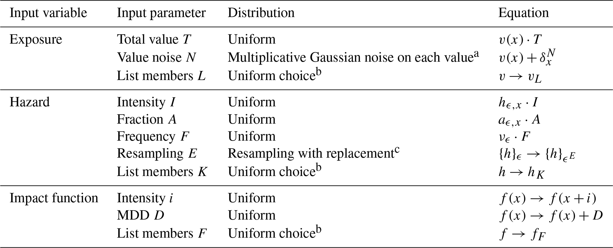
Table B2Summary of available helper methods to define uncertainty parameter distributions for the additional input variables of CLIMADA required for appraisal of adaptation options. For all distributions, the parameters can be set by the user (e.g. the bounds of the uniform distributions are free parameters). * The discount rate value is sampled uniformly from a list of values. These helper methods are for the convenience of the users only. Any other uncertainty parameter distributions (discrete, continuous, multi-dimensional, etc.) can be defined by the user if needed.

In the Vietnam case study Rana et al. (2022), hazard datasets of probabilistic tropical cyclones for storm surges were created for the period 1980−2020, based on 269 historical, land-falling events recorded in the global International Best Track Archive for Climate Stewardship (IBTrACS) (Knapp et al., 2010). These historical tropical cyclone records were extended using a random walk algorithm to produce 99 probabilistic tracks for each record, yielding a large set of synthetic events (Kleppek et al., 2008; Gettelman et al., 2017; Aznar-Siguan and Bresch, 2019). A 2D wind-field was calculated for each track using the wind model after Holland (2008). The surge hazard dataset (flood depth) is derived from wind intensity with a linear relationship that modifies the water level according to the local elevation and distance to the coastal line, as further described in Rana et al. (2022). Future climate hazard sets were created for two Relative Concentration Pathways (RCP) (IPCC, 2014a), RCP6.0 and RCP8.5, based on parametric estimates. For each storm, the intensity and frequency where homogeneously shifted by a multiplicative constant derived from Knutson et al. (2015) based on the storm's Saffir–Simpson category.
The spatial distribution of population was obtained from the LitPop module in CLIMADA at a resolution of 1 km and using the population census data only, i.e. (Eberenz et al., 2020). For the future scenario, a total population growth is estimated to amount to 13 % until 2050 based on estimates from the United United Nations, Department of Economic and Social Affairs, Population Division (2019). The impact function for the effect of storm surges on population was created in consultation with experts in the field; all people are considered affected at 1 m water depth (Rana et al., 2022). Benefit and cost information on the three adaptation measures (sea dykes, gabions, mangroves) are given in Table 3. in Rana et al. (2022).
As stated in Sect. 4, not all quantifiable uncertainties are described with the quasi-Monte Carlo method discussed in this paper. For instance, the uncertainty in climate risk arising from the inherent stochasticity of weather events can be directly described without using the unsequa module. In CLIMADA, this variability is directly modelled by considering the hazard to be a probabilistic set of events, i.e. intensity maps with associated frequencies (Aznar-Siguan and Bresch, 2019). Computing the risk from the hazard amounts to computing the risk for each event in the set, which results in a probabilistic risk distribution. The event risk distribution expresses the fact that we do not know when a particular natural hazard event will happen, and qualifies as aleatory uncertainty (Uusitalo et al., 2015; Ghanem et al., 2017). One can compute statistical values, such as the mean or standard deviation, or consider the full distribution over the event set as shown in Fig. D8a for the original case study risk. There is no need for an extra sampling (and use of the unsequa module) to determine this uncertainty, as this is part of the modelling of the hazard. Note however, that this variability is itself subject to modelling uncertainty. The distribution of risk obtained over all events and all input parameter samples, as shown in Fig. D8b, can then be seen as an estimate of the weather risk variability, including additional uncertainties.
Note that in general, global uncertainty and sensitivity analyses as discussed in this paper apply only to deterministic computer codes, i.e. models for which a specific set of input values always results in the same output (Saltelli et al., 2008; Marrel et al., 2012). CLIMADA is such a deterministic computer code. In order to describe truly stochastic models, we would have to use other techniques, for instance, techniques that allow us to consider correlations between input parameters, or which are directly built for probabilistic computer codes (Ehre et al., 2020; Étoré et al., 2020; Zhu and Sudret, 2021).
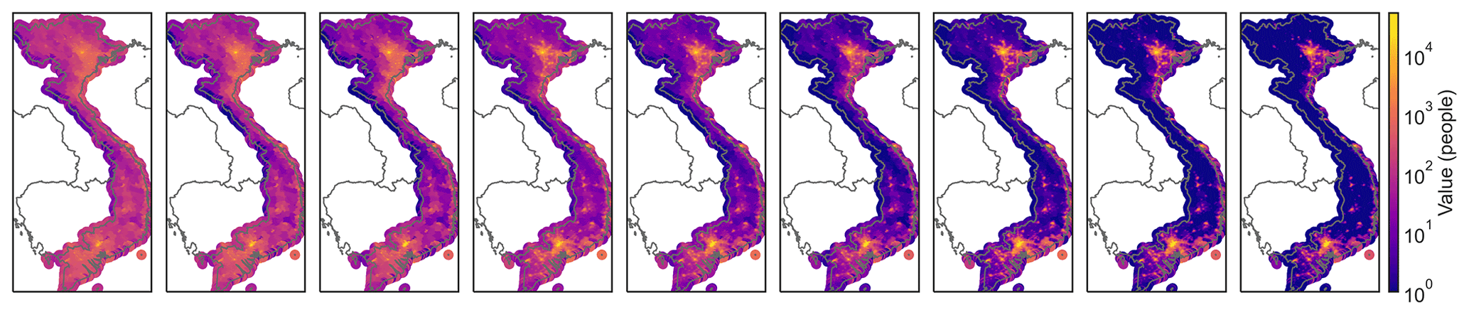
Figure D1Population distribution obtained by combining population density layer and nightlight satellite imagery (cf. Litpop method, Eberenz et al., 2020) for all combinations of the nightlight and population exponents m and n considered in the uncertainty analysis (cf. Table 1). From left to right, m,n = (0, 0.75); (0, 1); (0, 1.25); (0.5, 0.75); (0.5, 1); (0.5, 1.25); (1, 0.75); (1, 1); (1, 1.25), with (0, 1) the original case study value.
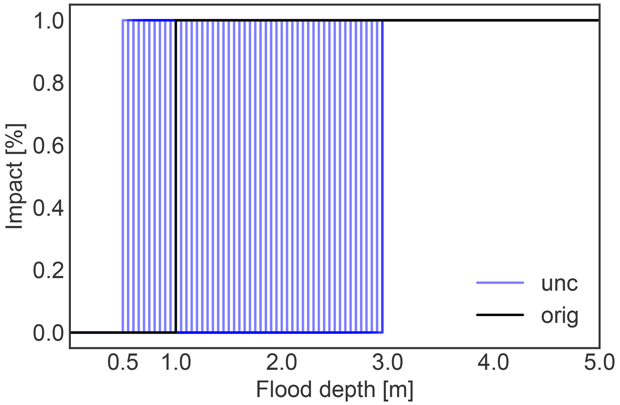
Figure D2Impact function uncertainty, with a threshold shift of the flood depth above which all people are affected varying between 0.5 and 3 m (cf. Table 1). The original impact function is given in black.
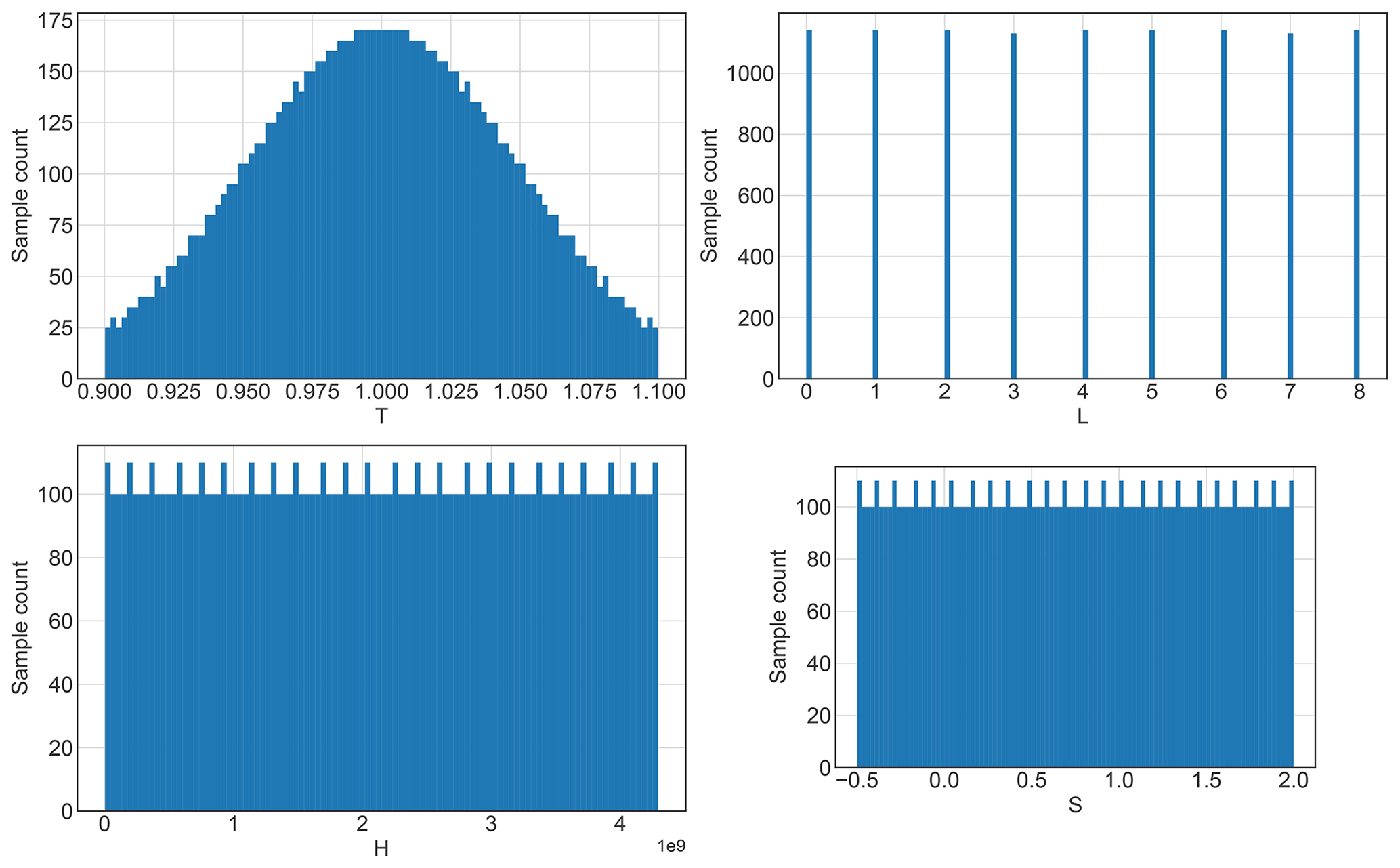
Figure D3Samples for the uncertainty analysis of the risk assessment in Sect. 3.2.2 for the input parameters drawn from the distributions described in Table 1 using the sequence. The input parameters are T: total population, L: population L: population distribution, S: impact function threshold shift, and H: hazard events bootstrapping.
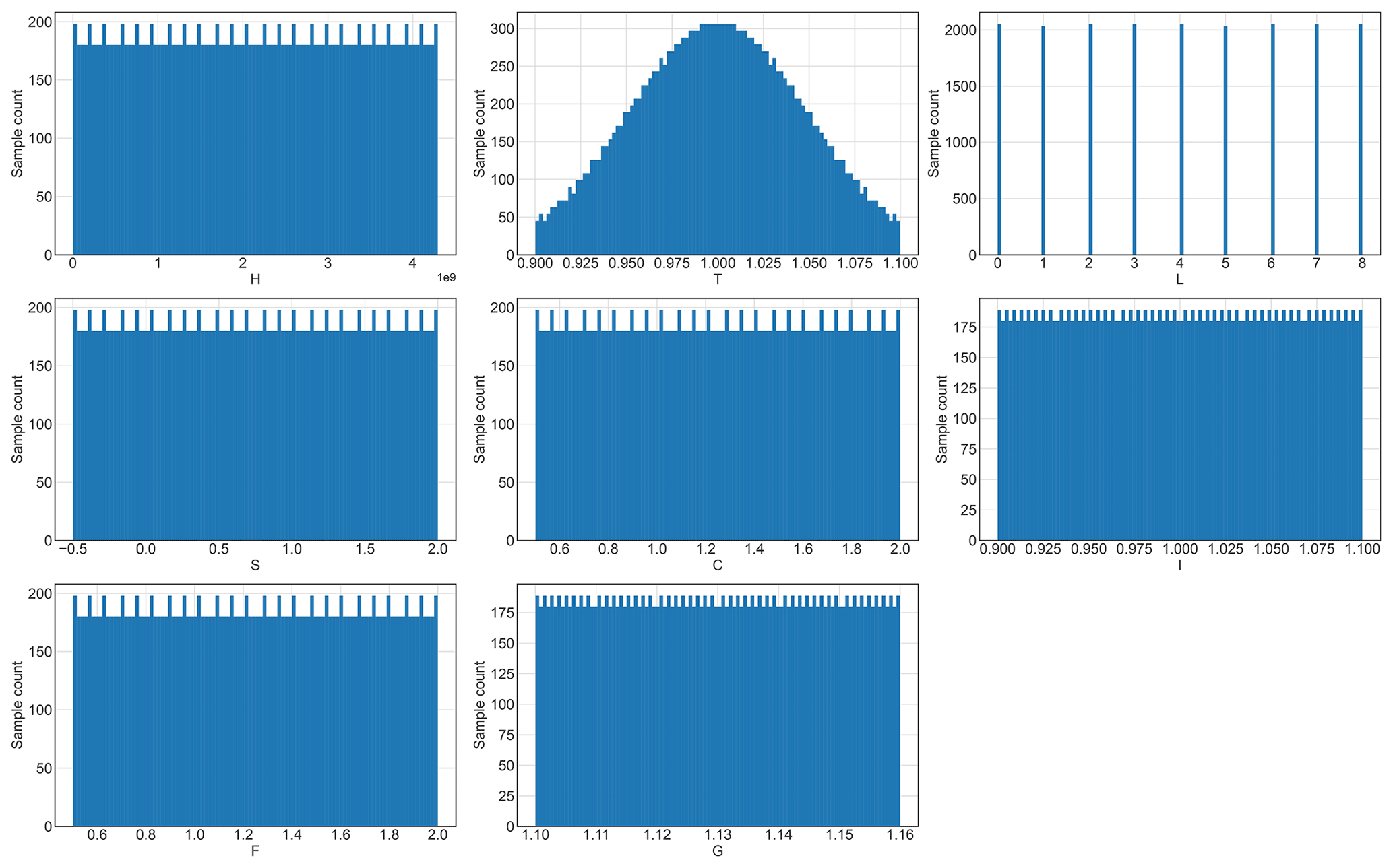
Figure D4Samples for the uncertainty analysis of the adaptation options appraisal in Sect. 3.2.2 for the input parameters drawn from the distributions described in Table 1 using the Sobol′ sequence. The input parameters are H: hazard events bootstrapping, T: total population, L: population distribution, S: impact function intensity threshold shift, C: cost of adaptation options, I: hazard intensity change, F: hazard frequency change, and G: population growth.
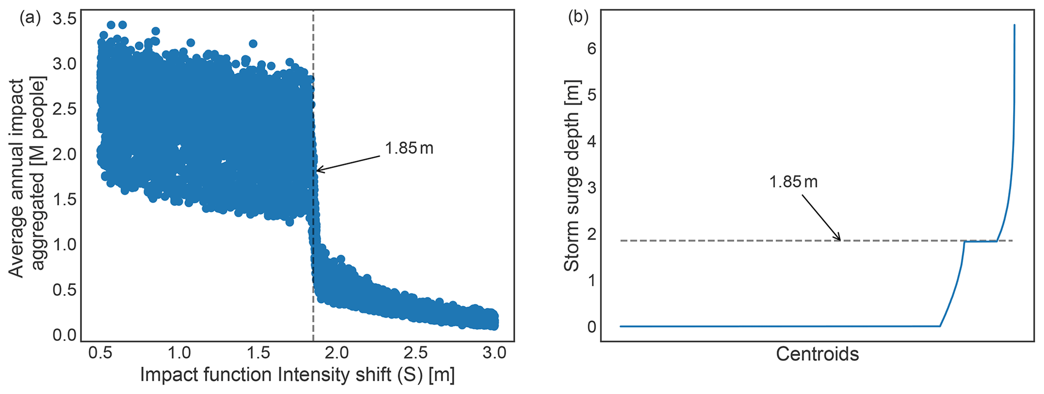
Figure D5(a) Annual average impact averaged over all exposure points in millions (M) of affected people as a function of the impact function threshold shift uncertainty (S) in metres (m), and (b) storm surge intensity in metres (m) of all events at each location (centroid) from the original case study. A nonlinear change in intensity at ∼1.85 m is indicated by a dashed line.

Figure D6Second-order Sobol′ sensitivity indices (S2) for different storm surge risk metrics: average annual impact aggregated over all exposure points (aai_agg), impact for return periods (rp) years and the total exposure value (tot_value). The input parameters (cf. Table 1) are T: total population, L: population distribution, S: impact function intensity threshold shift, and H: hazard events bootstrapping.

Figure D7Uncertainty distribution (histogram bars) for the ratio of cost to benefit of the three adaptation options (a) mangroves, (b) sea dykes, and (c) gabions. In addition, (d) the total-order Sobol′ sensitivity indices (ST) for the three adaptation options. Panels of cost to benefit ratios include the original case study value (vertical dotted green line), average (vertical dashed orange line), standard deviation (horizontal solid black line), and kernel density estimation to guide the eye (solid dark-blue The total-order Sobol' sensitivities are shown with a black bar bar indicating the 95th percentile confidence interval. The input parameters (cf. Table 1) are H: hazard events bootstrapping, T: total population, L: population distribution, S: impact function intensity threshold shift, C: cost of adaptation options, I: hazard intensity change, F: hazard frequency change, and G: population growth.
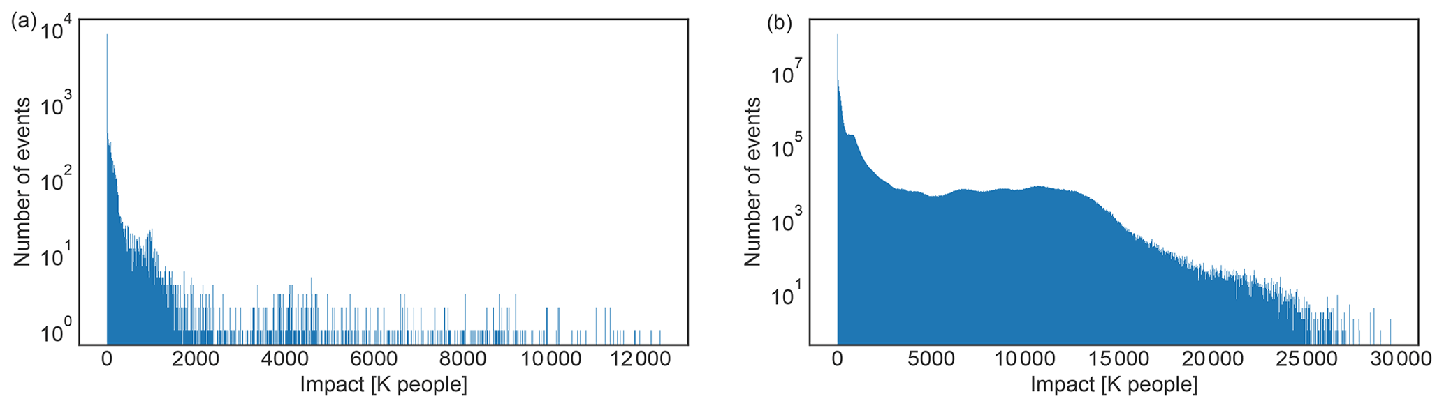
Figure D8Histogram of the number of storm surge events in the probabilistic set by their impact (in thousands (K) of affected people) in Vietnam for present climate conditions (2020) for (a) the original case study probabilistic set, and (b) union of the probabilistic sets for all samples of input parameters considered in Sect. 3.2.4 (cf. Fig. D3). Note the logarithmic scale of the vertical axes.
CLIMADA is openly available at GitHub https://github.com/CLIMADA-project/climada_python (last access: 30 August 2022), and https://doi.org/10.5281/zenodo.5947271 (Kropf et al., 2022a) under the GNU GPL license (GNU operating system, 2007). The documentation is hosted on Read the Docs https://climada-python.readthedocs.io/en/stable/ (last access: 30 August 2022) and includes a link to the interactive tutorial of CLIMADA. In this publication, CLIMADA v3.1.0, deposited on Zenodo (Kropf et al., 2022a) was used.).
All data have been generated using CLIMADA (the LitPop exposures, the impact function, the storm surge hazard, the adaptation measures, all impact and cost–benefit values, the uncertainty distributions, and the sensitivity indices). Detailed tutorials are available at https://climada-python.readthedocs.io/en/v3.1.1/ (last access: 30 August 2022) (version 3.1.) and at https://climada-python.readthedocs.io/en/stable/ (last access: 30 August 2022) (latest stable version). For generating the storm surge hazard in 2020 and 2050, a digital elevation model (DEM) was used which is not included in CLIMADA. The hazards have been made available under the DOI https://doi.org/10.3929/ethz-b-000566528 (Kropf et al., 2022b). The scripts to reproduce all other data in this paper are available at https://github.com/CLIMADA-project/climada_papers (a frozen version was deposited at https://doi.org/10.3929/ethz-b-000566528).
Conceptualization was by CMK, AC, SM, DNB, ES, LO, and JWM; writing of the original draft was by CMK and AC; writing – review and editing – was by CMK, AC, SM, DNB, ES, LO, JWM, and AR; data curation was by CMK and AR; formal analysis was by CMK; software was the responsibility of CMK and ES; resources were managed by DNB; visualization was by CMK and AC; project administration was by CMK.
The contact author has declared that none of the authors has any competing interests.
Publisher's note: Copernicus Publications remains neutral with regard to jurisdictional claims in published maps and institutional affiliations.
The authors are grateful to Moustapha Maliki and Evelyn Mühlhofer for valuable discussion at the start of this project.
This research has been supported by Horizon 2020 (CASCADES (grant no. 821010) and RECEIPT (grant no. 820712)).
This paper was edited by Christian Folberth and reviewed by Francesca Pianosi and Nadia Bloemendaal.
Anderson, W., Guikema, S., Zaitchik, B., and Pan, W.: Methods for Estimating Population Density in Data-Limited Areas: Evaluating Regression and Tree-Based Models in Peru, PLOS ONE, 9, e100037, https://doi.org/10.1371/journal.pone.0100037, 2014. a
Aznar-Siguan, G. and Bresch, D. N.: CLIMADA v1: a global weather and climate risk assessment platform, Geosci. Model Dev., 12, 3085–3097, https://doi.org/10.5194/gmd-12-3085-2019, 2019. a, b, c, d, e, f, g, h, i, j
Berger, L.: Leaving No One Off The Map: A Guide For Gridded Population Data For Sustainable Development, A Report by the Thematic Research Network on Data and Statistics (TReNDS) of the UN Sustainable Development Solutions Network (SDSN) in Support of the POPGRID Data Collaborative, https://www.unsdsn.org/leaving-no-one-off-the-map-a-guide-for-gridded-population-data-for-sustainable-development (last access: 28 August 2022), 2020. a
Beven, K. J., Almeida, S., Aspinall, W. P., Bates, P. D., Blazkova, S., Borgomeo, E., Freer, J., Goda, K., Hall, J. W., Phillips, J. C., Simpson, M., Smith, P. J., Stephenson, D. B., Wagener, T., Watson, M., and Wilkins, K. L.: Epistemic uncertainties and natural hazard risk assessment – Part 1: A review of different natural hazard areas, Nat. Hazards Earth Syst. Sci., 18, 2741–2768, https://doi.org/10.5194/nhess-18-2741-2018, 2018. a, b
Beven, K. J., Aspinall, W. P., Bates, P. D., Borgomeo, E., Goda, K., Hall, J. W., Page, T., Phillips, J. C., Simpson, M., Smith, P. J., Wagener, T., and Watson, M.: Epistemic uncertainties and natural hazard risk assessment – Part 2: What should constitute good practice?, Nat. Hazards Earth Syst. Sci., 18, 2769–2783, https://doi.org/10.5194/nhess-18-2769-2018, 2018b. a, b
Bloemendaal, N., Haigh, I. D.,de Moel, H., Muis, S., Haarsma, R. J., and Aerts, J. C. J. H.: Generation of a Global Synthetic Tropical Cyclone Hazard Dataset Using STORM, Sci. Data, 7, 40, https://doi.org/10.1038/s41597-020-0381-2, 2020. a
Borgonovo, E.: A New Uncertainty Importance Measure, Reliab. Eng. Syst. Safe., 92, 771–784, https://doi.org/10.1016/j.ress.2006.04.015, 2007. a
Borgonovo, E., Lu, X., Plischke, E., Rakovec, O., and Hill, M. C.: Making the Most out of a Hydrological Model Data Set: Sensitivity Analyses to Open the Model Black-Box, Water Resour. Res., 53, 7933–7950, https://doi.org/10.1002/2017WR020767, 2017. a
Bradley, R. and Drechsler, M.: Types of Uncertainty, Erkenn, 79, 1225–1248, https://doi.org/10.1007/s10670-013-9518-4, 2014. a, b
Bradley, R. and Steele, K.: Making Climate Decisions, Philosophy Compass, 10, 799–810, https://doi.org/10.1111/phc3.12259, 2015. a, b
Bresch, D. N. and Aznar-Siguan, G.: CLIMADA v1.4.1: towards a globally consistent adaptation options appraisal tool, Geosci. Model Dev., 14, 351–363, https://doi.org/10.5194/gmd-14-351-2021, 2021. a, b, c, d, e, f
Center for International Earth Science Information Network (CIESIN): Documentation for the Gridded Population of the World, Version 4 (GPWv4), Revision 10 Data Sets [data set], https://doi.org/10.7927/H4D50JX4, 2017. a
Ceola, S., Laio, F., and Montanari, A.: Satellite Nighttime Lights Reveal Increasing Human Exposure to Floods Worldwide, Geophys. Res. Lett., 41, 7184–7190, https://doi.org/10.1002/2014GL061859, 2014. a
Ciullo, A., Kwakkel, J. H., Bruijn, K. M. D., Doorn, N., and Klijn, F.: Efficient or Fair? Operationalizing Ethical Principles in Flood Risk Management: A Case Study on the Dutch-German Rhine, Risk Anal., 40, 1844–1862, https://doi.org/10.1111/risa.13527, 2020. a
Ciullo, A., Martius, O., Strobl, E., and Bresch, D. N.: A Framework for Building Climate Storylines Based on Downward Counterfactuals: The Case of the European Union Solidarity Fund, Climate Risk Management, 33, 100349, https://doi.org/10.1016/j.crm.2021.100349, 2021. a
Cukier, R. I., Fortuin, C. M., Shuler, K. E., Petschek, A. G., and Schaibly, J. H.: Study of the Sensitivity of Coupled Reaction Systems to Uncertainties in Rate Coefficients. I Theory, J. Chem. Phys., 59, 3873–3878, https://doi.org/10.1063/1.1680571, 1973. a
de Moel, H., Asselman, N. E. M., and Aerts, J. C. J. H.: Uncertainty and sensitivity analysis of coastal flood damage estimates in the west of the Netherlands, Nat. Hazards Earth Syst. Sci., 12, 1045–1058, https://doi.org/10.5194/nhess-12-1045-2012, 2012. a
Doorn, N.: The Blind Spot in Risk Ethics: Managing Natural Hazards, Risk Anal., 35, 354–360, https://doi.org/10.1111/risa.12293, 2015. a
Dottori, F., Di Baldassarre, G., and Todini, E.: Detailed Data Is Welcome, but with a Pinch of Salt: Accuracy, Precision, and Uncertainty in Flood Inundation Modeling, Water Resour. Res., 49, 6079–6085, https://doi.org/10.1002/wrcr.20406, 2013. a, b
Douglas-Smith, D., Iwanaga, T., Croke, B. F. W., and Jakeman, A. J.: Certain Trends in Uncertainty and Sensitivity Analysis: An Overview of Software Tools and Techniques, Environ. Modell. Softw., 124, 104588, https://doi.org/10.1016/j.envsoft.2019.104588, 2020. a, b
Eberenz, S., Stocker, D., Röösli, T., and Bresch, D. N.: Asset exposure data for global physical risk assessment, Earth Syst. Sci. Data, 12, 817–833, https://doi.org/10.5194/essd-12-817-2020, 2020. a, b, c, d, e
Ehre, M., Papaioannou, I., and Straub, D.: A Framework for Global Reliability Sensitivity Analysis in the Presence of Multi-Uncertainty, Reliab. Eng. Syst. Safe., 195, 106726, https://doi.org/10.1016/j.ress.2019.106726, 2020. a
Emanuel, K.: A Fast Intensity Simulator for Tropical Cyclone Risk Analysis, Nat. Hazards, 88, 779–796, https://doi.org/10.1007/s11069-017-2890-7, 2017. a
Étoré, P., Prieur, C., Pham, D. K., and Li, L.: Global Sensitivity Analysis for Models Described by Stochastic Differential Equations, Methodol. Comput. Appl. Probab., 22, 803–831, https://doi.org/10.1007/s11009-019-09732-6, 2020. a
Funtowicz, S. O. and Ravetz, J. R.: Uncertainty and Quality in Science for Policy, Springer Science & Business Media, https://doi.org/10.1007/978-94-009-0621-1, 1990. a
Gettelman, A., Bresch, D. N., Chen, C. C., Truesdale, J. E., and Bacmeister, J. T.: Projections of Future Tropical Cyclone Damage with a High-Resolution Global Climate Model, Climatic Change, 146, 575–585, https://doi.org/10.1007/s10584-017-1902-7, 2017. a
Ghanem, R., Higdon, D., and Owhadi, H.: Handbook of Uncertainty Quantification, Springer, New York, NY, 1st Edn., https://doi.org/10.1007/978-3-319-11259-6, 2017. a
Hall, J. W., Tarantola, S., Bates, P. D., and Horritt, M. S.: Distributed Sensitivity Analysis of Flood Inundation Model Calibration, J. Hydraul. Eng., 131, 117–126, https://doi.org/10.1061/(ASCE)0733-9429(2005)131:2(117), 2005. a
Hammersley, J. M.: Monte Carlo Methods for Solving Multivariable Problems, Ann. NY Acad. Sci., 86, 844–874, https://doi.org/10.1111/j.1749-6632.1960.tb42846.x, 1960. a
Herman, J. and Usher, W.: SALib: An Open-Source Python Library for Sensitivity Analysis, J. Open Source Softw., 2, 97, https://doi.org/10.21105/joss.00097, 2017. a, b, c, d, e
Hillger, D., Seaman, C., Liang, C., Miller, S., Lindsey, D., and Kopp, T.: Suomi NPP VIIRS Imagery Evaluation, J. Geophys. Res.-Atmos., 119, 6440–6455, https://doi.org/10.1002/2013JD021170, 2014. a
Hinkel, J. and Bisaro, A.: Methodological Choices in Solution-Oriented Adaptation Research: A Diagnostic Framework, Reg. Environ. Change, 16, 7–20, https://doi.org/10.1007/s10113-014-0682-0, 2016. a, b
Holland, G.: A Revised Hurricane Pressure–Wind Model, Mon. Wea. Rev., 136, 3432–3445, https://doi.org/10.1175/2008MWR2395.1, 2008. a
Hyde, K. M.: Uncertainty Analysis Methods For Multi-Criteria Decision Analysis, PhD thesis, The University of Adelaide School of Civil and Environmental Engineering, Adelaide, 2006. a
IFRC: World Disasters Rreport: Come Heat or High Water., INTL FED OF RED CROSS, GENEVA, ISBN 978-2-9701289-5-3, https://media.ifrc.org/ifrc/world-disaster-report-2020 (last access: 28 August 2022), 2020. a
Iooss, B. and Lemaître, P.: A Review on Global Sensitivity Analysis Methods, in: Uncertainty Management in Simulation-Optimization of Complex Systems: Algorithms and Applications, edited by: Dellino, G. and Meloni, C., Operations Research/Computer Science Interfaces Series, Springer US, Boston, MA, 101–122, https://doi.org/10.1007/978-1-4899-7547-8_5, 2015. a
IPCC: Climate Change 2014: Synthesis Report. Contribution of Working Groups I, II and III to the Fifth Assessment Report of the Intergovernmental Panel on Climate Change, edited by: Core Writing Team, Pachauri, R. K., and Meyer, L. A., IPCC, Geneva, Switzerland, 151 pp., https://www.ipcc.ch/report/ar5/syr/ (last access: 28 August 2022), 2014a. a, b, c
IPCC: 2014: Summary for policymakers, in: Climate Change 2014: Impacts, Adaptation, and Vulnerability. Part A: Global and Sectoral Aspects. Contribution of Working Group II to the Fifth Assessment Report of the Intergovernmental Panel on Climate Change, edited by: Field, C. B., Barros, V. R., Dokken, D. J., Mach, K. J., Mastrandrea, M. D., Bilir, T. E., Chatterjee, M., Ebi, K. L., Estrada, Y. O., Genova, R. C., Girma, B., Kissel, E. S., Levy, A. N., MacCracken, S., Mastrandrea, P. R., and White, L. L., Cambridge University Press, Cambridge, United Kingdom and New York, NY, USA, 1–32, https://www.ipcc.ch/report/ar5/wg2/ (last access: 28 August 2022), 2014b. a
IPCC: Climate Change 2021: The Physical Science Basis. Contribution of Working Group I to the Sixth Assessment Report of the Intergovernmental Panel on Climate Change, edited by: Masson-Delmotte, V., Zhai, P., Pirani, A., Connors, S. L., Péan, C., Berger, S., Caud, N., Chen, Y., Goldfarb, L., Gomis, M. I., Huang, M., Leitzell, K., Lonnoy, E., Matthews, J. B. R., Maycock, T. K., Waterfield, T., Yelekçi, O., Yu, R., and Zhou, B., Cambridge University Press, Cambridge, United Kingdom and New York, NY, USA, 2391 pp., https://www.ipcc.ch/report/ar6/wg1/ (last access: 28 August 2022), 2021. a
Kam, P. M., Aznar-Siguan, G., Schewe, J., Milano, L., Ginnetti, J., Willner, S., McCaughey, J. W., and Bresch, D. N.: Global Warming and Population Change Both Heighten Future Risk of Human Displacement Due to River Floods, Environ. Res. Lett., 16, 044026, https://doi.org/10.1088/1748-9326/abd26c, 2021. a
Kasprzyk, J. R., Nataraj, S., Reed, P. M., and Lempert, R. J.: Many Objective Robust Decision Making for Complex Environmental Systems Undergoing Change, Environ. Modell. Softw., 42, 55–71, https://doi.org/10.1016/j.envsoft.2012.12.007, 2013. a
Katzav, J., Thompson, E. L., Risbey, J., Stainforth, D. A., Bradley, S., and Frisch, M.: On the appropriate and inappropriate uses of probability distributions in climate projections and some alternatives, Climatic Change, 169, 15, https://doi.org/10.1007/s10584-021-03267-x, 2021. a
Kleppek, S., Muccione, V., Raible, C. C., Bresch, D. N., Köllner-Heck, P., and Stocker, T. F.: Tropical Cyclones in ERA-40: A Detection and Tracking Method, Geophys. Res. Lett., 35, L10705, https://doi.org/10.1029/2008GL033880, 2008. a
Knapp, K. R., Kruk, M. C., Levinson, D. H., Diamond, H. J., and Neumann, C. J.: The International Best Track Archive for Climate Stewardship (IBTrACS): Unifying Tropical Cyclone Data, B. Am. Meteorol. Soc., 91, 363–376, https://doi.org/10.1175/2009BAMS2755.1, 2010. a
Knüsel, B.: Epistemological Issues in Data-Driven Modeling in Climate Research, Doctoral Thesis, ETH Zurich, https://doi.org/10.3929/ethz-b-000399735, 2020. a, b
Knüsel, B., Baumberger, C., Zumwald, M., Bresch, D. N., and Knutti, R.: Argument-Based Assessment of Predictive Uncertainty of Data-Driven Environmental Models, Environ. Modell. Softw., 134, 104754, https://doi.org/10.1016/j.envsoft.2020.104754, 2020. a, b, c, d, e, f, g
Knutson, T. R., Sirutis, J. J., Zhao, M., Tuleya, R. E., Bender, M., Vecchi, G. A., Villarini, G., and Chavas, D.: Global Projections of Intense Tropical Cyclone Activity for the Late Twenty-First Century from Dynamical Downscaling of CMIP5/RCP4.5 Scenarios, J. Climate, 28, 7203–7224, https://doi.org/10.1175/JCLI-D-15-0129.1, 2015. a, b
Koks, E. E., Bočkarjova, M., de Moel, H., and Aerts, J. C. J. H.: Integrated Direct and Indirect Flood Risk Modeling: Development and Sensitivity Analysis, Risk Anal., 35, 882–900, https://doi.org/10.1111/risa.12300, 2015. a
Krauß, W. and Bremer, S.: The Role of Place-Based Narratives of Change in Climate Risk Governance, Climate Risk Manage., 28, 100221, https://doi.org/10.1016/j.crm.2020.100221, 2020. a
Kropf, C. M., Schmid, E., Aznar-Siguan, G., Eberenz, S., Vogt, T., Steinmann, C. B., Röösli, T., Lüthi, S., Sauer, I. J., Mühlhofer, E., Hartman, J., Guillod, B. P., Stalhandske, Z., Ciullo, A., Fairless, C., Kam, P. M. M., wjan262, Meiler, S., Bungener, R., Bozzini, V., Stocker, D., and Bresch, D. N.: CLIMADA-project/Climada_python: V3.1.0, Zenodo [code], https://doi.org/10.5281/zenodo.5947271, 2022a. a, b, c, d
Kropf, C. M., Rana, A., and Zhu, Q.: Probabilistic storm surge hazard event set for Vietnam on 30 arcsecond resolution (2020 and 2050), ETH Research Collection [code and data set], https://doi.org/10.3929/ethz-b-000566528, 2022b. a
Lemieux, C.: Monte Carlo and Quasi-Monte Carlo Sampling, Springer Science & Business Media, https://doi.org/10.1007/978-0-387-78165-5, 2009. a, b, c
Leobacher, G. and Pillichshammer, F.: Introduction to Quasi-Monte Carlo Integration and Applications, Springer, https://doi.org/10.1007/978-3-319-03425-6, 2014. a, b
Marelli, S. and Sudret, B.: UQLab: A Framework for Uncertainty Quantification in Matlab, in: Second International Conference on Vulnerability and Risk Analysis and Management (ICVRAM) and the Sixth International Symposium on Uncertainty, Modeling, and Analysis (ISUMA), American Society of Civil Engineers, Liverpool, 2554–2563, https://doi.org/10.1061/9780784413609.257, 2014. a
Marrel, A., Iooss, B., Da Veiga, S., and Ribatet, M.: Global Sensitivity Analysis of Stochastic Computer Models with Joint Metamodels, Stat. Comput., 22, 833–847, https://doi.org/10.1007/s11222-011-9274-8, 2012. a
Matott, L. S., Babendreier, J. E., and Purucker, S. T.: Evaluating Uncertainty in Integrated Environmental Models: A Review of Concepts and Tools, Water Resour. Res., 45, W06421, https://doi.org/10.1029/2008WR007301, 2009. a, b
Mayer, L. A., Loa, K., Cwik, B., Tuana, N., Keller, K., Gonnerman, C., Parker, A. M., and Lempert, R. J.: Understanding Scientists' Computational Modeling Decisions about Climate Risk Management Strategies Using Values-Informed Mental Models, Global Environ. Chang., 42, 107–116, https://doi.org/10.1016/j.gloenvcha.2016.12.007, 2017. a, b
Merwade, V., Olivera, F., Arabi, M., and Edleman, S.: Uncertainty in Flood Inundation Mapping: Current Issues and Future Directions, J. Hydrol. Eng., 13, 608–620, https://doi.org/10.1061/(ASCE)1084-0699(2008)13:7(608), 2008. a, b
Moeller, J.: Distributive Justice and Climate Change: The What, How, and Who Fo Climate Change Policy, Graduate Student Theses, Dissertations, & Professional Papers, 2016. a, b
Morris, M. D.: Factorial Sampling Plans for Preliminary Computational Experiments, Technometrics, 33, 161–174, https://doi.org/10.1080/00401706.1991.10484804, 1991. a
Norton, J.: An introduction to sensitivity assessment of simulation models, Environ. Modell. Softw., 69, 166–174, https://doi.org/10.1016/j.envsoft.2015.03.020, 2015. a
Otth, L.: Analyzing the Sensitivity of Climate Impact Model Outputs to Ethical and Epistemic Uncertainties, Master Thesis, ETH Zurich, https://doi.org/10.3929/ethz-b-000525807, 2021. a, b, c, d, e, f
Otth, L., Rüegsegger, C., Kropf, C. M., Ciullo, A., Meiler, S., Bresch, D. N., and McCaughey, J. W.: Analyzing Uncertainties in Climate Risk Assessment and Adaptation Options Appraisal with a Four-Phase Analytical Framework, submitted, 2022. a, b, c, d, e, f
Paleari, L. and Confalonieri, R.: Sensitivity Analysis of a Sensitivity Analysis: We Are Likely Overlooking the Impact of Distributional Assumptions, Ecol. Modell., 340, 57–63, https://doi.org/10.1016/j.ecolmodel.2016.09.008, 2016. a, b
Pianosi, F. and Wagener, T.: A Simple and Efficient Method for Global Sensitivity Analysis Based on Cumulative Distribution Functions, Environ. Modell. Softw., 67, 1–11, https://doi.org/10.1016/j.envsoft.2015.01.004, 2015. a
Pianosi, F., Beven, K., Freer, J., Hall, J. W., Rougier, J., Stephenson, D. B., and Wagener, T.: Sensitivity Analysis of Environmental Models: A Systematic Review with Practical Workflow, Environ. Modell. Softw., 79, 214–232, https://doi.org/10.1016/j.envsoft.2016.02.008, 2016. a, b, c, d, e, f
Plischke, E., Borgonovo, E., and Smith, C. L.: Global Sensitivity Measures from given Data, Eur. J. Oper. Res., 226, 536–550, https://doi.org/10.1016/j.ejor.2012.11.047, 2013. a
Rana, A., Zhu, Q., Detken, A., Whalley, K., and Castet, C.: Strengthening climate-resilient development and transformation in Viet Nam, Climatic Change, 170, 4, https://doi.org/10.21203/rs.3.rs-1050224/v1, 2022. a, b, c, d, e, f, g, h, i, j
Saltelli, A.: Making Best Use of Model Evaluations to Compute Sensitivity Indices, Comput. Phys. Commun., 145, 280–297, https://doi.org/10.1016/S0010-4655(02)00280-1, 2002. a
Saltelli, A., Ratto, M., Andres, T., Campolongo, F., Cariboni, J., Gatelli, D., Saisana, M., and Tarantola, S.: Global Sensitivity Analysis: The Primer, John Wiley & Sons, Ltd, Chichester, England, Hoboken, NJ, ISBN 9780470059975, Online ISBN 9780470725184, https://doi.org/10.1002/9780470725184, 2008. a, b, c
Saltelli, A. and Annoni, P.: How to Avoid a Perfunctory Sensitivity Analysis, Environ. Modell. Softw., 25, 1508–1517, https://doi.org/10.1016/j.envsoft.2010.04.012, 2010. a, b, c
Saltelli, A., Guimaraes Pereira, Â., der Sluijs, J. P. V., and Funtowicz, S.: What Do I Make of Your Latinorumc Sensitivity Auditing of Mathematical Modelling, International Journal of Foresight and Innovation Policy, 9, 213, https://doi.org/10.1504/IJFIP.2013.058610, 2013. a
Saltelli, A., Aleksankina, K., Becker, W., Fennell, P., Ferretti, F., Holst, N., Li, S., and Wu, Q.: Why so Many Published Sensitivity Analyses Are False: A Systematic Review of Sensitivity Analysis Practices, Environ. Modell. Softw., 114, 29–39, https://doi.org/10.1016/j.envsoft.2019.01.012, 2019. a, b, c, d
Sarrazin, F. J., Pianosi, F., and Wagener, T.: Global Sensitivity Analysis of Environmental Models: Convergence and Validation, Environ. Modell. Softw., 79, 135–152, https://doi.org/10.1016/j.envsoft.2016.02.005, 2016. a, b
Savage, J. T. S., Pianosi, F., Bates, P., Freer, J., and Wagener, T.: Quantifying the Importance of Spatial Resolution and Other Factors through Global Sensitivity Analysis of a Flood Inundation Model, Water Resour. Res., 52, 9146–9163, https://doi.org/10.1002/2015WR018198, 2016. a
Shepherd, T. G., Boyd, E., Calel, R. A., Chapman, S. C., Dessai, S., Dima-West, I. M., Fowler, H. J., James, R., Maraun, D., Martius, O., Senior, C. A., Sobel, A. H., Stainforth, D. A., Tett, S. F. B., Trenberth, K. E., van den Hurk, B. J. J. M., Watkins, N. W., Wilby, R. L., and Zenghelis, D. A.: Storylines: An Alternative Approach to Representing Uncertainty in Physical Aspects of Climate Change, Climatic Change, 151, 555–571, https://doi.org/10.1007/s10584-018-2317-9, 2018. a
Sobol′, I. M.: Global Sensitivity Indices for Nonlinear Mathematical Models and Their Monte Carlo Estimates, Math. Comput. Simulat., 55, 271–280, https://doi.org/10.1016/S0378-4754(00)00270-6, 2001. a, b, c, d, e
Sobol′, I. M. and Kucherenko, S.: Derivative Based Global Sensitivity Measures and Their Link with Global Sensitivity Indices, Mathe. Comput. Simulat., 79, 3009–3017, https://doi.org/10.1016/j.matcom.2009.01.023, 2009. a
Souvignet, M., Wieneke, F., Müller, L., and Bresch, D. N.: Economics of Climate Adaptation (ECA): Guidebook for Practitioners, KfW Group, KfW Development Bank, Frankfurt am Main, https://www.kfw-entwicklungsbank.de/PDF/Download-Center/Materialien/2016_No6_Guidebook_Economics-of-Climate-Adaptation_EN.pdf (last access: 28 August 2022), 2016. a
Sudret, B.: Global Sensitivity Analysis Using Polynomial Chaos Expansions, Reliab. Eng. Syst. Safe., 93, 964–979, https://doi.org/10.1016/j.ress.2007.04.002, 2008. a
United Nations, Department of Economic and Social Affairs, Population Division: World Population Prospects 2019: Data Booklet (ST/ESA/SER.A/424), https://population.un.org/wpp/ (last access: 28 August 2022), 2019. a, b, c
Uusitalo, L., Lehikoinen, A., Helle, I., and Myrberg, K.: An Overview of Methods to Evaluate Uncertainty of Deterministic Models in Decision Support, Environ. Modell. Softw., 63, 24–31, https://doi.org/10.1016/j.envsoft.2014.09.017, 2015. a
Van Rossum, G. and Drake, F. L.: Python 3 Reference Manual, CreateSpace, Scotts Valley, CA, ISBN 978-1-4414-1269-0, 2009. a
Virtanen, P., Gommers, R., Oliphant, T. E., Haberland, M., Reddy, T., Cournapeau, D., Burovski, E., Peterson, P., Weckesser, W., Bright, J., van der Walt, S. J., Brett, M., Wilson, J., Millman, K. J., Mayorov, N., Nelson, A. R. J., Jones, E., Kern, R., Larson, E., Carey, C. J., Polat, İ., Feng, Y., Moore, E. W., VanderPlas, J., Laxalde, D., Perktold, J., Cimrman, R., Henriksen, I., Quintero, E. A., Harris, C. R., Archibald, A. M., Ribeiro, A. H., Pedregosa, F., and van Mulbregt, P.: SciPy 1.0: Fundamental Algorithms for Scientific Computing in Python, Nat. Methods, 17, 261–272, https://doi.org/10.1038/s41592-019-0686-2, 2020. a
Wagenaar, D. J., de Bruijn, K. M., Bouwer, L. M., and de Moel, H.: Uncertainty in flood damage estimates and its potential effect on investment decisions, Nat. Hazards Earth Syst. Sci., 16, 1–14, https://doi.org/10.5194/nhess-16-1-2016, 2016. a
Wagener, T., Reinecke, R., and Pianosi, F.: On the Evaluation of Climate Change Impact Models, WIREs Clim. Change, 13, e772, https://doi.org/10.1002/wcc.772, 2022. a
Wilby, R. L. and Dessai, S.: Robust Adaptation to Climate Change, Weather, 65, 180–185, https://doi.org/10.1002/wea.543, 2010. a
Zhu, X. and Sudret, B.: Global Sensitivity Analysis for Stochastic Simulators Based on Generalized Lambda Surrogate Models, Reliab. Eng. Syst. Safe., 214, 107815, https://doi.org/10.1016/j.ress.2021.107815, 2021. a
“Impacts generally refer to effects on lives; livelihoods; health and well-being; ecosystems and species; economic, social and cultural assets; services (including ecosystem services); and infrastructure. Impacts may be referred to as consequences or outcomes, and can be adverse or beneficial.” (IPCC, 2014b)
In literature, the terminology “input factor” instead of “input parameter” is also used. Here we shall exclusively use the terminology “input parameter” for numerical random variables, and “input variable” for the inputs to the CLIMADA model.
- Abstract
- Introduction
- Uncertainty and sensitivity analyses in the climate-risk modelling platform CLIMADA
- Illustration with a case study on tropical cyclones storm surges in Vietnam
- Discussion and outlook
- Appendix A: Sampling algorithms
- Appendix B: Helper methods
- Appendix C: Case study details
- Appendix D: Event uncertainty
- Code availability
- Data availability
- Author contributions
- Competing interests
- Disclaimer
- Acknowledgements
- Financial support
- Review statement
- References