the Creative Commons Attribution 4.0 License.
the Creative Commons Attribution 4.0 License.
 | 27 Jul 2022
Integrated Methane Inversion (IMI 1.0): a user-friendly, cloud-based facility for inferring high-resolution methane emissions from TROPOMI satellite observations
Daniel J. Varon
Daniel J. Jacob
Melissa Sulprizio
Lucas A. Estrada
William B. Downs
Lu Shen
Sarah E. Hancock
Hannah Nesser
Elise Penn
Zichong Chen
Alba Lorente
Ashutosh Tewari
Cynthia A. Randles
We present a user-friendly, cloud-based facility for quantifying methane emissions with 0.25∘ × 0.3125∘ (≈ 25 km × 25 km) resolution by inverse analysis of satellite observations from the TROPOspheric Monitoring Instrument (TROPOMI). The facility is built on an Integrated Methane Inversion optimal estimation workflow (IMI 1.0) and supported for use on the Amazon Web Services (AWS) cloud. It exploits the GEOS-Chem chemical transport model and TROPOMI data already resident on AWS, thus avoiding cumbersome big-data download. Users select a region and period of interest, and the IMI returns an analytical solution for the Bayesian optimal estimate of period-average emissions on the 0.25∘ × 0.3125∘ grid including error statistics, information content, and visualization code for inspection of results. The inversion uses an advanced research-grade algorithm fully documented in the literature. An out-of-the-box inversion with rectilinear grid and default prior emission estimates can be conducted with no significant learning curve. Users can also configure their inversions to infer emissions for irregular regions of interest, swap in their own prior emission inventories, and modify inversion parameters. Inversion ensembles can be generated at minimal additional cost once the Jacobian matrix for the analytical inversion has been constructed. A preview feature allows users to determine the TROPOMI information content for their region and time period of interest before actually performing the inversion. The IMI is heavily documented and is intended to be accessible by researchers and stakeholders with no expertise in inverse modelling or high-performance computing. We demonstrate the IMI's capabilities by applying it to estimate methane emissions from the US oil-producing Permian Basin in May 2018.
- Article
(4438 KB) - Full-text XML
- BibTeX
- EndNote


Cynthia A. Randles's and Ashutosh Tewari's copyrights for this publication are transferred to ExxonMobil Technology and Engineering Company.
Controlling methane emissions is a major focus of climate policy (EC and USA, 2021). Anthropogenic methane emissions are primarily from livestock, oil and gas operations, coal mining, waste management, and rice cultivation (Saunois et al., 2020). Emission inventories use “bottom-up” methods to estimate emissions from activity levels and emission factors in these different sectors, but the emission factors are often highly uncertain (IPCC, 2019). “Top-down” inverse methods using satellite observations of atmospheric methane in combination with an atmospheric transport model and statistical optimization can evaluate the bottom-up inventories and monitor emissions worldwide, but they are difficult to use and have their own errors (Jacob et al., 2016).
Here we present an open-access, cloud-based facility for researchers and stakeholders to estimate methane emissions for user-selected regions of interest by performing high-resolution analytical inversions of TROPOspheric Monitoring Instrument (TROPOMI) satellite data archived on the cloud and including quality control and error characterization as part of the inversion results. This facility enables users to infer methane emissions from TROPOMI data without requiring expert knowledge of inverse methods or cumbersome data download. It exemplifies the emerging concept of “bringing compute to data” that is viewed as crucial for effective utilization of very large Earth science datasets (Yang et al., 2017).
Satellite instruments observe atmospheric methane column concentrations by solar backscatter in the shortwave infrared (SWIR). Earlier instruments (SCIAMACHY, GOSAT) demonstrated effectiveness for inferring methane emissions on large regional scales (Bergamaschi et al., 2013; Wecht et al., 2014; Turner et al., 2015; Miller et al., 2019) but were limited by coarse pixel resolution (SCIAMACHY, 2003–2012) or sparse sampling (GOSAT, 2009–present). TROPOMI, launched in October 2017 aboard the European Space Agency's Sentinel-5P satellite, offers unprecedented capability for monitoring emissions on regional scales, with daily global observations at 5.5 km × 7 km nadir pixel resolution over land (Hu et al., 2018; Schneising et al., 2019; Lorente et al., 2021). The retrieval success rate averages only 3 % because of clouds and dark and heterogeneous surfaces (Hasekamp et al., 2019), but the data density is still at least 2 orders of magnitude higher than for GOSAT (Qu et al., 2021). TROPOMI data have been used in regional inversions at up to 25 km resolution (Zhang et al., 2020; Shen et al., 2021, 2022; Z. Chen et al., 2022).
Inverse analysis of TROPOMI data to infer methane emissions requires a chemical transport model (CTM), known as forward model for the inversion, to relate emissions to the observed methane columns through simulation of atmospheric transport. The problem is generally underconstrained because of uneven data density and because of errors in the satellite retrievals and in the CTM, referred to collectively as observational error. The solution must therefore be regularized, typically with prior information in the form of bottom-up emissions on the CTM grid, to produce posterior emission estimates that improve on the prior. This is generally done by minimization of a Bayesian cost function, using either variational methods or an analytical solution (Brasseur and Jacob, 2017). Variational methods can infer methane emissions on any grid, for any nonlinear problem, and for any error probability density function (pdf), but they do not immediately provide error characterization of the posterior estimate. An analytical solution takes advantage of the linearity of the relationship between methane emissions and concentrations (Chen and Prinn, 2006; Maasakkers et al., 2021). It requires explicit construction of the Jacobian matrix expressing the sensitivity of concentrations to emissions, but this is readily done on supercomputing clusters as an embarrassingly parallel problem (Maasakkers et al., 2019). Two major advantages of the analytical solution are that (1) it provides closed-form characterizations of the posterior error pdf and the information content of the observations, and (2) it allows easy generation of solution ensembles exploring the inversion parameter space (Lu et al., 2022).
Inverse analysis of satellite observations requires complex modelling tools, advanced data processing, and access to high-end computational resources. These are major barriers for novice and occasional users and for stakeholders lacking technical expertise. Our user-friendly, cloud-based facility for inferring high-resolution methane emissions from TROPOMI satellite data lifts those barriers. The facility is based on an Integrated Methane Inversion workflow (IMI 1.0) that builds on current best practices for analytical inversion of TROPOMI data (Shen et al., 2021). It draws on the GEOS-Chem CTM already accessible on the Amazon Web Services (AWS) cloud (Zhuang et al., 2019, 2020), directly accesses the operational TROPOMI data maintained on the cloud by Meteorological Environmental Earth Observation S.r.l. (MEEO), and infers methane emissions at 0.25∘ × 0.3125∘ (≈ 25 km × 25 km) resolution for user-selected regions. It is designed to be easily configurable for users wishing to quantify emissions for specific regions and periods. The workflow can be run “out of the box” or modified with user-supplied information, and it can be downloaded for users who wish to work on their own computational clusters. Our objective in this paper is to provide a high-level description of the facility and exemplify its practical use. Detailed technical documentation for user support is available online (https://imi.seas.harvard.edu, last access: 8 June 2022).
The IMI infers methane emissions for a user-selected region and period by inverse analysis of TROPOMI methane observations with GEOS-Chem as forward model. The forward model F relates the period-average methane emissions (gridded state vector x) to the observed methane columns (observation vector y) such that , where the observational error εo includes errors in both the satellite data and the forward model. The inversion optimizes x to match the observations, subject to constraints from the prior emission estimates (xa), which have their own error εa. The optimization is done by analytical minimization of a least-squares Bayesian cost function, yielding a posterior estimate for the state vector with accompanying error statistics. Here we describe the different components of the IMI and use a 1-month inversion for the US Permian Basin (Fig. 1) as a guiding example.
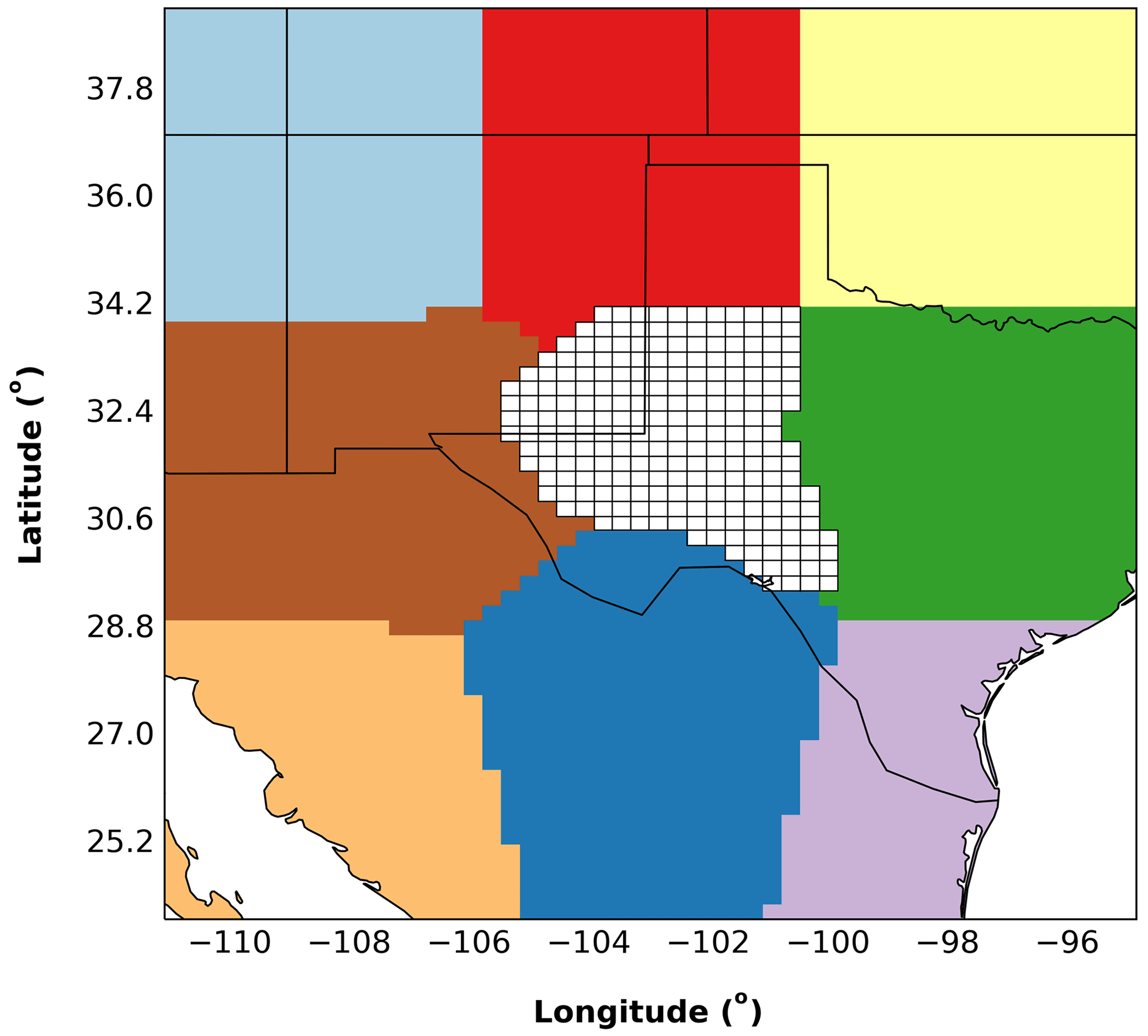
Figure 1Example of an IMI state vector for inferring methane emissions from TROPOMI observations. Here the region of interest is the US Permian Basin in Texas and New Mexico (grid with white background), comprising 235 grid elements at 0.25∘ × 0.3125∘ resolution generated from a shapefile. The inversion domain also includes the areas in color bordering the region of interest, representing eight buffer elements added to the state vector to correct errors in boundary conditions (see Sect. 2.3).
2.1 TROPOMI satellite observations
TROPOMI retrieves atmospheric methane columns from backscattered sunlight in the 2.3 µm methane absorption band, with daily global coverage at 5.5 km × 7 km nadir pixel resolution (7 km × 7 km prior to August 2019). Measurements are made at ∼ 13:30 local solar time. The methane retrieval is produced by the Netherlands Institute for Space Research (SRON). It is based on the RemoTeC full-physics algorithm (Butz et al., 2009, 2010, 2011) and retrieves methane data as column-average dry-air mixing ratios (ppb) along with surface reflectivity and scattering properties of the atmosphere (Butz et al., 2012; Hu et al., 2016). The TROPOMI data are posted operationally on the AWS cloud and updated daily by MEEO with a latency of a few days (https://registry.opendata.aws/sentinel5p, last access: 8 June 2022). The methane product provides information on numerous retrieval parameters together with , including the center and boundaries of the pixel, the surface pressure, the 12-layer pressure grid of the retrieval, the vertical averaging kernel vector and prior vertical profile of methane dry-air mixing ratio, a quality assurance value, and the retrieved surface albedo in the near-infrared (NIR) and SWIR spectral ranges.
The operational TROPOMI record begins in May 2018. The methane retrieval is presently Version 1 (Hasekamp et al., 2019) until July 2021 and Version 2 (Lorente et al., 2021) afterward. Validation of Version 1.3.0 showed a global mean bias of −2.7 ppb relative to ground-based measurements from 19 sites in the Total Column Carbon Observing Network (TCCON; Wunch et al., 2011a; Qu et al., 2021), but global bias is of no consequence for regional inversions because it is effectively corrected through the boundary conditions. Of more concern are spatially variable biases (regional biases), caused mainly by aliasing of surface albedo errors into the methane retrieval (Lorente et al., 2021) but also by scattering-induced surface reflectance errors (Barré et al., 2021) and errors in surface altitude (Hachmeister et al., 2022). Qu et al. (2021) quantified a nominal TROPOMI regional bias of 6.7 ppb in Version 1.3.0 as the standard deviation of station-to-station biases between TROPOMI and the 19 TCCON sites, and a similar analysis for Version 2.2.0 shows a regional bias of 5.6 ppb (Lorente et al., 2021). This is sufficiently small to enable successful regional inversions, for which Buchwitz et al. (2015) estimated a regional bias threshold of 10 ppb. In the IMI we only use recommended high-quality retrievals over land, with quality assurance value ≥ 0.5 (Hu et al., 2016). We further remove observations with low SWIR albedo (< 0.05; de Gouw et al., 2020) and high “blended albedo” (> 0.85), a linear combination of NIR and SWIR albedo, to avoid biases from dark and snow-covered scenes (Wunch et al., 2011b; Lorente et al., 2021). The quantity of data removed by these additional filters depends on the region and period for the inversion; we find for example that they remove roughly 25 % (summer) to 40 % (winter) of otherwise high-quality observations across North America in 2019.
2.2 GEOS-Chem chemical transport model as forward model for the inversion
GEOS-Chem is a three-dimensional CTM that simulates methane concentrations on the basis of prescribed emissions either globally or for user-selected nested domains (Wecht et al., 2014). It is driven by Goddard Earth Observation System (GEOS) meteorological data from the NASA Global Modelling and Assimilation Office (GMAO). The IMI uses as default the GEOS Fast Processing (GEOS-FP) meteorological data product at 0.25∘ × 0.3125∘ resolution, with an option to use the GEOS Modern-Era Retrospective Analysis for Research and Applications, version 2 (MERRA-2) at 0.5∘ × 0.625∘ resolution. The GEOS data have 72 vertical levels from the surface to the mesopause, and these are condensed to 47 levels in our GEOS-Chem simulations by merging levels in the upper stratosphere and mesosphere.
We use the nested capability of GEOS-Chem to simulate methane concentrations over the inversion domain, with dynamic boundary conditions outside the inversion domain updated every 3 h from a global archive of TROPOMI data smoothed spatially over a rolling ± 10∘ window and temporally over a 1-month period centered on each grid square and day and distributed vertically following a GEOS-Chem simulation at 4∘ × 5∘ resolution (Shen et al., 2021). This smoothed TROPOMI 3-D archive is provided as part of the IMI. Using smoothed TROPOMI data as boundary conditions minimizes bias from boundary conditions advected over the user-selected region. Smoothing of the TROPOMI data is necessary because of the sparsity of successful retrievals and the noise therein. To further reduce the bias associated with boundary conditions, we expand the inversion domain beyond the user-selected region of interest to include a buffer area, and coarse buffer elements are added to the state vector of methane emissions to be optimized (Fig. 1, Sect. 2.3).
The user-specified period of interest defines the time window for the GEOS-Chem simulation. Starting from the smoothed TROPOMI fields as initial conditions, we apply a 1-month spin-up with prior emission estimates to properly initialize the model concentration fields within the inversion domain; 1 month is sufficient to fully ventilate any practical regional domain. This spin-up only needs to be done once.
The GEOS-Chem simulation includes chemical methane sinks from archived (offline) tropospheric concentrations of oxidants (OH, Cl) and stratospheric loss frequencies (Maasakkers et al., 2019), as well as soil uptake (Murguia-Flores et al., 2018), but these are inconsequential for nested-domain simulations and are not optimized by the IMI. Ventilation of the inversion domain takes place on much shorter timescales than the methane atmospheric lifetime, and the sinks are relatively spatially smooth, so no information on methane sinks is to be gained from a regional inversion. The effect of methane sinks is implicitly included in the specification of boundary conditions.
2.3 Methane emission state vector to be optimized
The state vector x is the ensemble of variables (“state variables”) to be optimized in the inversion. In the IMI, these are the gridded methane emissions (temporal mean) at 0.25∘ × 0.3125∘ resolution for the region and period of interest, plus buffer elements at coarser resolution bordering the region of interest and filling out the inversion domain (eight elements by default). Users specify a region and time period of interest in the IMI configuration file. The region of interest can have any irregular shape, as illustrated in Fig. 1. In that example case, the region of interest is an assemblage of 235 0.25∘ × 0.3125∘ grid cells covering the geological extent of the Permian Basin, and the eight buffer elements expand to a rectangular inversion domain 24–39∘ N, 95–111∘ W. The state vector in this example has length .
The simplest (default) option for the user is to select a rectangular region of interest as latitude and longitude bounds. The IMI then infers emissions for the 0.25∘ × 0.3125∘ grid cells within that region, excluding any grid cells less than 25 % over land (adjustable default), and selects eight additional buffer elements with a k-means algorithm to pad out the rectangular inversion domain. The k-means algorithm sorts grid cells by latitude–longitude coordinates, and the number of buffer elements can be adjusted in the configuration file. Users also have the option to select an irregular region of interest, as in the Permian example of Fig. 1, by providing a previously defined state vector file or a shapefile for the region boundaries. Offshore emissions can be included in the state vector by lowering the default 25 % land cover requirement or by directly modifying the state vector file. TROPOMI does not observe over water except in the glint mode, but information on offshore emissions can still be gained from the plumes transported over nearby land (Shen et al., 2021).
Table 1Bottom-up methane emission inventories used as default prior estimates in IMI 1.0 a.
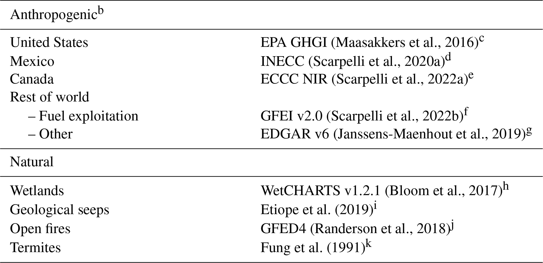
a The inventories are archived on AWS on their native grids and over their temporal records and are re-gridded and summed for use as IMI prior estimates through the Harmonized Emissions Component (HEMCO) emissions processor in GEOS-Chem (Lin et al., 2021). The inventories listed here are those available as of January 2022. They will be updated in the future as improved or more recent emission inventory data become available. Users can also substitute their own inventories. b All anthropogenic emissions are on a 0.1∘ × 0.1∘ grid and resolved by emission sector. They do not vary with time of year except for manure (Maasakkers et al., 2016) and rice (Zhang et al., 2021). c Gridded version of the US EPA Inventory of US Greenhouse Gas Emissions and Sinks (GHGI; EPA, 2016) for 2012. d Gridded version of the Instituto Nacional de Ecología y Cambio Climático (INECC) national inventory (INECC and SEMARNAT, 2018) for 2015. e Gridded version of the Environment and Climate Change Canada (ECCC) National Inventory Report (NIR; ECCC, 2020) for 2018. f Global Fuel Emission Inventory (GFEI v2) constructed by gridding the national sectoral emission inventories reported by individual countries to the UNFCCC for 2018 and 2019. g Data for 2018. h Emissions for individual years and months specified on a 0.5∘ × 0.5∘ grid from the mean of the WetCHARTs ensemble. i Scaled to a global total emission of 1.6 Tg a−1 (Hmiel et al., 2020). j Daily emissions specified on a 0.25∘ × 0.25∘ grid from the Global Fire Emissions Database (GFED4). k Emissions specified on a 4∘ × 5∘ grid.
2.4 Prior emission estimates
The prior emission estimates xa should represent the best knowledge of methane emissions prior to performing the inversion. They need to be available in gridded format to match the resolution of the inversion. Table 1 compiles the bottom-up emission inventories used as default prior estimates in the IMI. The North American anthropogenic emissions are gridded versions of the national sector-resolved inventories reported by the individual countries to the United Nations Framework Convention on Climate Change (UNFCCC) as given by Maasakkers et al. (2016) for the United States, Scarpelli et al. (2020a) for Mexico, and Scarpelli et al. (2022a) for Canada. The emissions from fuel exploitation (oil, gas, coal) in the rest of the world similarly grid the national emissions reported annually to the UNFCCC (Scarpelli et al., 2022b). The Emission Database for Global Atmospheric Research (EDGAR) v6 is otherwise used as the global default. Natural emissions include contributions from wetlands with monthly resolution (Bloom et al., 2017), open fires with daily resolution (Randerson et al., 2018), and small sources from geological seeps and termites. These default inventories can be superseded by users with their own prior estimates, and we give an example of this in Sect. 4.
The inversion infers emissions on the 0.25∘ × 0.3125∘ grid, and this may include contributions from different sectors. Users can attribute the corrections to individual sectors based on the sectoral distribution of the emissions in the prior inventories and estimates of prior errors for each sector (Shen et al., 2021; Cusworth et al., 2021a). This needs to be done in post-processing of the inversion results.
2.5 TROPOMI operator
The forward model y=F(x) for the inversion involves successive application of a GEOS-Chem operator C=G(x) that relates the emission state vector x to the resulting 3-D simulated dry-air mixing ratio field C and a TROPOMI operator y=T(C) that relates the vertical profile of simulated dry-air mixing ratios to the corresponding column-average dry-air mixing ratio () that would be observed by TROPOMI. The TROPOMI retrieval provides information on the operator T as the dependence of on the local vertical profile vector of dry-air mixing ratios c (with prior estimate ca) for 12 sub-column pressure layers extending from the local surface to the top of the atmosphere, with vertical sensitivity described by a column-averaging kernel vector η for those 12 layers:
where 1 denotes a 12-dimensional unit vector.

Figure 2Simulation of TROPOMI column-average dry-air mixing ratio () observations in the GEOS-Chem 3-D model atmosphere. (a) The operator first identifies which GEOS-Chem grid cells overlap with the TROPOMI observation pixel. (b) The operator remaps conservatively the GEOS-Chem vertical profile of methane dry sub-column mixing ratios cG from the GEOS-Chem pressure grid pG to the TROPOMI pressure grid pT to produce a vertical profile of methane sub-column mixing ratios cT on the TROPOMI pressure grid. (c) The TROPOMI averaging kernel vector η (Eq. 1) is applied to the remapped GEOS-Chem profile on the TROPOMI pressure grid to produce a virtual observation of the GEOS-Chem atmosphere. If multiple GEOS-Chem grid cells overlap with the TROPOMI observation, the corresponding values are area-weighted to the TROPOMI pixel.
Figure 2 summarizes the operations involved in simulating TROPOMI observations of the GEOS-Chem atmosphere. The first step is to geo-locate the TROPOMI pixel (nadir resolution 5.5 km × 7 km, but coarser off-nadir) on the GEOS-Chem 0.25∘ × 0.3125∘ grid, including the region of interest and the surrounding buffer elements. If the pixel overlaps two or more GEOS-Chem grid cells then the calculation is done for each grid cell column followed by area-weighted averaging. We remap the sub-column mixing ratios from the GEOS-Chem vertical grid (47 layers) to the TROPOMI vertical grid (12 layers) with total or partial allocation of GEOS-Chem layers to TROPOMI layers on the basis of pressure edges (Fig. 2). We then apply the TROPOMI column-averaging kernel vector η with Eq. (1) to obtain the column-average dry-air mixing ratio as would be observed by TROPOMI in the GEOS-Chem atmosphere. When remapping GEOS-Chem to the TROPOMI vertical grid, we address differences in surface pressure between GEOS-Chem and TROPOMI by adjusting the lowest GEOS-Chem pressure edge to match that of TROPOMI, as illustrated in Fig. 2; this applies the lowest-level sub-column mixing ratio in GEOS-Chem down to the lowest TROPOMI pressure edge.
The column-averaging kernel sensitivities in TROPOMI are generally within 2 % of unity in the troposphere and drop off slowly in the stratosphere (Hu et al., 2016). Thus the pressure remapping has relatively little effect except in regions with strong topography, where high-elevation pixels have greater stratospheric contribution to . Stanevich et al. (2020) reported that stratospheric methane in GEOS-Chem exhibits a high bias relative to ACE-FTS satellite observations, but Zhang et al. (2021) found that this bias is largely restricted to polar vortex conditions where TROPOMI does not have observations.
2.6 Optimization procedure
Our Bayesian inversion to infer methane emissions fits the GEOS-Chem simulation to the TROPOMI observations, weighing prior and observational uncertainties and assuming normal error pdf's. This involves minimization of the scalar cost function (Brasseur and Jacob, 2017)
where is the Jacobian matrix, Sa is the prior error covariance matrix, So is the observational error covariance matrix including contributions from instrument and forward model errors, and γ is an additional regularization parameter. K describes the sensitivity of observations y to the state vector x as described by the forward model F(x). It is computed column by column from an ensemble of perturbation simulations in the forward model, each perturbing a single element of the state vector from the reference simulation. Because the model is strictly linear, K defines GEOS-Chem for the purpose of the inversion.
The default Sa is constructed in the IMI by assuming 50 % error standard deviation on emissions, with no error correlations (diagonal matrix). The default So assumes a uniform observational error standard deviation of 15 ppb, based on previous estimates of 13–15 ppb for TROPOMI by the residual error method (Qu et al., 2021; Shen et al., 2021), again with no error correlation. These default values are adjustable by the user through the configuration file. The assumption of uncorrelated prior errors may lead to underestimation of the aggregated error in total regional emissions.
The regularization parameter γ is used to prevent overfitting and underfitting that would result from inexact specifications of Sa and So and because the observations are not perfectly independent and identically distributed (IID condition). The best value for γ can be selected on the basis of the L curve (Hansen, 1999) or the expected Chi-square distribution of the cost function's prior terms (Lu et al., 2021). These two methods yield consistent results (Qu et al., 2021). Shen et al. (2021) used the L curve to select γ=0.25 for a regional inversion of TROPOMI observations over eastern Mexico at 0.25∘ × 0.3125∘ resolution. We adopt that value in the IMI as default, but it can be adjusted in configuration.
The posterior state vector minimizing J(x) is obtained by an analytical solution of as
with posterior error covariance matrix (characterizing uncertainty in ) given by
provides full closed-form characterization of the error in assuming that the inverse problem has been well posed through the formulation of the cost function. Errors in the formulation of the cost function can be evaluated through an inversion ensemble varying inversion parameters (e.g., γ), prior emission estimates, and satellite observation sampling. The averaging kernel matrix
describes the sensitivity of to the truth (i.e., ). The trace of A, referred to as the degrees of freedom for signal (DOFS; Rodgers, 2000), measures the information content of the observations towards optimizing the state vector. It represents the number of independent pieces of information on the state vector that the observations can quantify. The diagonal entries of A are referred to as averaging kernel sensitivities, and they give an estimate of how much the posterior solution for a given state vector element is informed by the observations as opposed to the prior estimates (Cui et al., 2014; Brasseur and Jacob, 2017). An emission element with averaging kernel sensitivity 0 is not quantified by the observations at all, and the inversion results for that grid cell return the prior value. An emission element with averaging kernel sensitivity 1 is fully quantified by the observations, and the inversion results for that grid cell are independent of the prior estimate. We use sparse matrix algebra for the matrix operations in Eqs. (3)–(5) so that the computational cost of the optimization procedure is small relative to the cost of constructing the Jacobian. Sample performance statistics are given in Sect. 3.7.
2.7 IMI preview: assessing information content before performing an inversion
The IMI includes a preview feature designed to help users avoid spending resources on inversions with insufficient information content. Lack of information could come from low TROPOMI data density (e.g., from cloud cover) and/or from seriously biased prior emission estimates for the region and period of interest. The preview can be run after configuring the IMI and before initiating the inversion, and it performs several tasks. First, it maps the TROPOMI data and prior emission estimates for the selected region and period of interest, so the user can assess spatial correspondence between the two datasets. Second, it maps observation density and counts the total number of observations available for the selected region and period. Third, it maps the SWIR albedo retrieved by TROPOMI to help users identify potential artifacts if the SWIR albedo and methane retrievals show similar features (Barré et al., 2021). Fourth, it estimates the USD financial cost of performing the inversion by scaling the cost of our illustrative Permian Basin inversion (Sect. 4.3) according to the number of state variables, grid resolution, and inversion period length. Finally, it makes a rough estimate of the expected DOFS for the user's inversion using the procedure outlined below. A detailed example of the IMI preview feature is presented in Sect. 4.2.
The rough estimate of the expected DOFS is done as follows. Ignoring error correlations, assuming uniform observational errors, and further assuming uniform transport, the calculation of the averaging kernel matrix reduces to a scalar problem (Brasseur and Jacob, 2017). The averaging kernel sensitivity A for a given emission element in the state vector is computed as
where σa () is the prior error standard deviation of the emission element, σo (mol mol−1) is the observational error standard deviation, m is the number of satellite observations relevant to that emission element, and the transport model is defined by the parameter k (m2 s kg−1) as a summary representation of the Jacobian. With default 50 % prior error standard deviation, we have ), where Qa (kg s−1) is the total prior emission for the region of interest, n is the number of emission elements in that region of interest, and L (m) is the grid cell side length (25 km in the GEOS-FP default). For our guiding Permian Basin example using the default IMI emission inventories, Qa = 1.1 Tg a−1, and n=235, which yields σa = 1.2 × 10⁻¹⁰ . The mean number of observations m per emission element is the total number of observations for the region and period of interest, divided by n; for the May 2018 Permian example we obtain m=86 from 19 978 observations (see Sect. 4.2). σo is by default 15 × 10−9 mol mol−1.
To estimate k we use the approximation proposed by Nesser et al. (2021) for simple mass balance ventilation of local emissions in the grid cell by a constant wind:
where Mair is the molar mass of dry air, is the molar mass of methane, g is gravitational acceleration, U is a uniform wind speed ventilating the emission element (assumed 5 km h−1), and p is the surface pressure (assumed 1010 hPa). The parameter α serves as a simple representation of turbulent diffusion, and here we take α=0.4 following Nesser et al. (2021) so that k = 1.26 m2 s kg−1. After computing A in this way, the expected information content for the inversion can be obtained as
Equation (8) gives a quick estimate of the information content to be expected from the inversion without actually performing the inversion. Although very rough, it is based on the same principles as the actual inversion, and we find that it gives a good approximation of the actual DOFS as demonstrated in Sect. 4.2. It further has the advantage of being transparent in that n and m are defined by the user choice of region and period of interest, σa and σo are set by default in the IMI but are configurable by the user, and k has direct physical meaning. In fact, k can be used for a very rough estimate of emissions corresponding to a local column enhancement (Jacob et al., 2016).
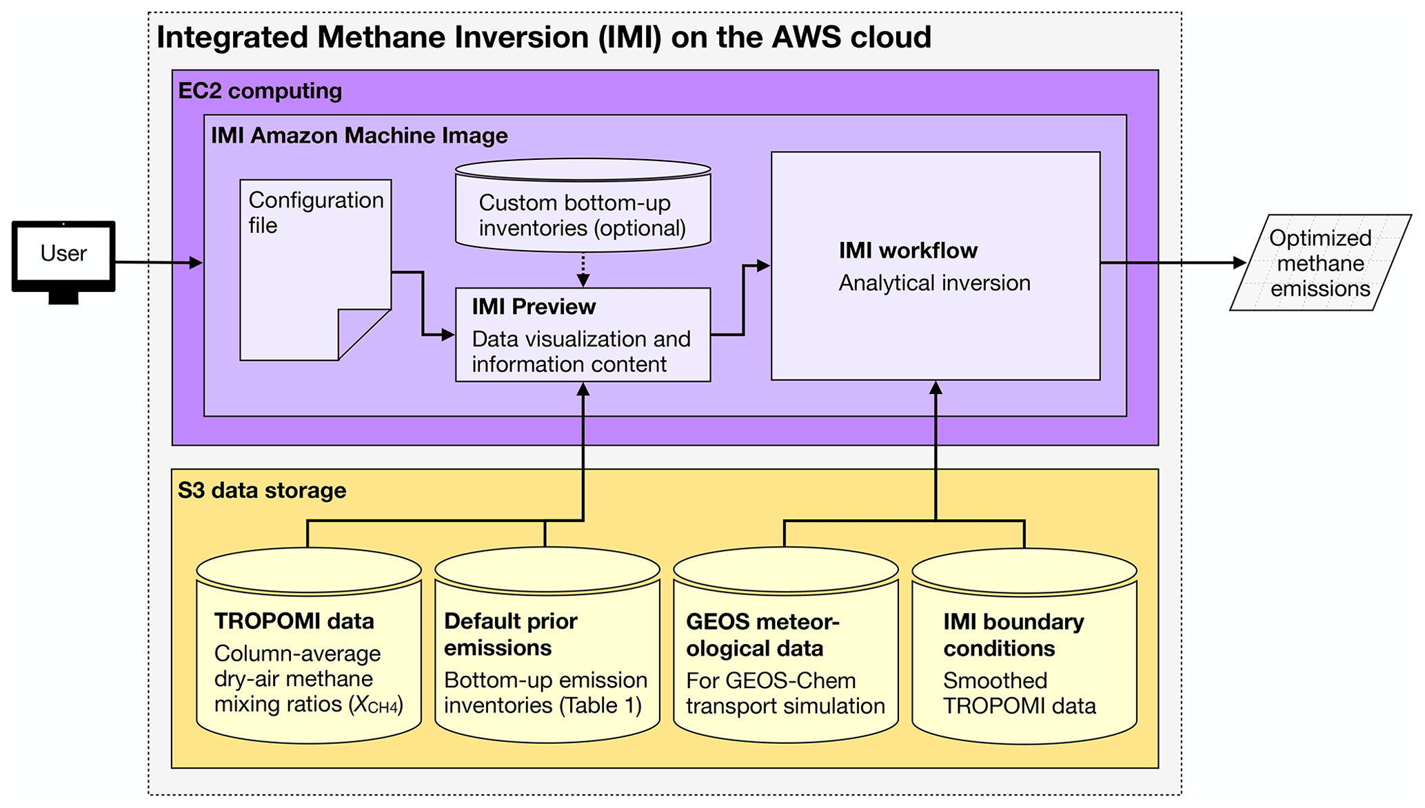
Figure 3Integrated Methane Inversion (IMI) preview and workflow on the Amazon Web Services (AWS) cloud to infer methane emissions from TROPOMI data. The IMI is accessed as a custom Amazon Machine Image (AMI) on the AWS EC2 computing service. It accesses the operational TROPOMI methane data, GEOS meteorological data, default bottom-up emission inventories, and IMI boundary conditions (smoothed TROPOMI data) from AWS S3 data storage buckets for the desired period. All of these data are resident on the cloud. Users specify their region or period of interest through a configuration file that also allows modification of IMI defaults. They can provide alternative bottom-up emission inventories (instead of the GEOS-Chem defaults) to serve as prior estimates for the inversion. The IMI preview provides visualization of the TROPOMI data and prior emission inventories and a rough estimate of the information content of the inversion (degrees of freedom for signal, or DOFS). Based on this information the user can decide to carry out the inversion through the IMI workflow (Fig. 4) or modify the configuration (see Sects. 2.7 and 4.2 for details).
The user may decide on the basis of the DOFS estimated from Eq. (8) whether or not to carry out the inversion. DOFS ∼ 1 would be a minimum requirement to achieve any solid information on emissions in the region of interest, and more may be desirable if multiple pieces of information are desired on the emission fields within the region. Shen et al. (2022) required DOFS > 2 to reliably estimate basin-wide emissions from oil and gas basins in North America. If the user deems the DOFS to be insufficient, a cure is to increase the number of observations by lengthening the observation period. The user may also revisit the information on the prior emission estimate and whether a larger value of σa may be appropriate, which will increase the DOFS.
Beyond inspection of the DOFS, the user should inspect the preview plots to guard against large artifacts in the observations or large bias in the spatial distribution of prior estimates. Artifacts in the observations can be diagnosed by similarity of patterns between and SWIR albedo, implying that spectral dependence of the albedo is propagating into the retrieval. If so the observations should not be used. Large bias in the spatial distribution of prior estimates can be diagnosed by comparison to the TROPOMI observations and would be problematic in the inversion by misallocating the corrections (Yu et al., 2021); this can be addressed by increasing the error in the prior estimate (including very large values to mimic a non-informative uniform prior) or switching to a different prior emission inventory, as is illustrated in Sect. 4 in the context of the Permian example.
Figure 3 outlines the architecture of the IMI on the AWS cloud including the preview and the inversion workflow. The IMI draws on two AWS facilities: the Elastic Compute Cloud (EC2) for computation and the Simple Storage Service (S3) for data storage. The computing environment for the workflow is contained in an Amazon Machine Image (AMI) accessible from the EC2 service. The TROPOMI operational data are archived independently in their own S3 bucket by MEEO. Meteorological data from the NASA GEOS-FP product are archived in another S3 bucket by the GEOS-Chem support team to support the general use of GEOS-Chem on the cloud (Zhuang et al., 2019). That bucket also contains the bottom-up methane emission inventories that serve as default prior estimates for the inversions (Table 1). Smoothed TROPOMI data serving as boundary conditions for the inversions are continuously updated by us to stay current with the TROPOMI operational data and have their own S3 bucket. All of these datasets are accessed by the preview and the workflow as needed, by automated transfer from S3 to the Elastic Block Store (EBS) volume on the user's EC2 instance.
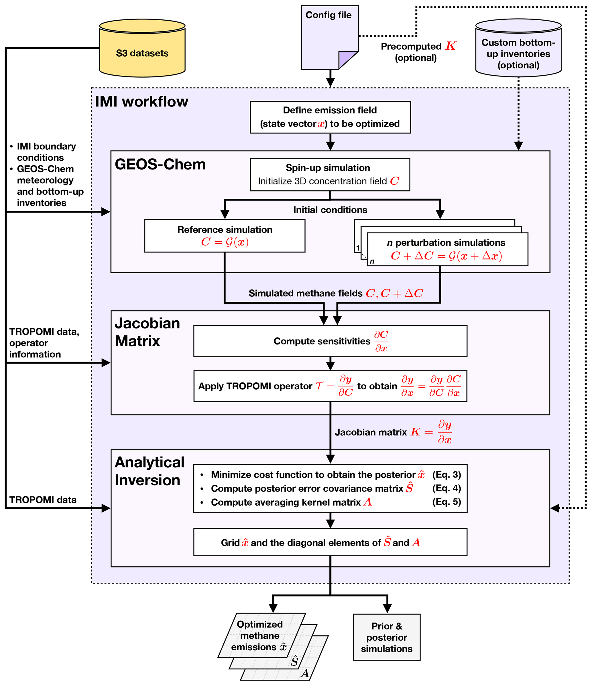
Figure 4Flowchart for the Integrated Methane Inversion (IMI 1.0) on the AWS cloud. Here x is the emission state vector of length n, y is the vector of TROPOMI observations, C is the time-evolving 3-D GEOS-Chem methane concentration field over the inversion period, G is the GEOS-Chem operator, T is the TROPOMI operator, K is the Jacobian matrix, is the posterior error covariance matrix, and A is the averaging kernel matrix. See Sect. 2 for equations and further description of the algorithm. The workflow has the option of skipping the calculation of the Jacobian matrix K if it has already been computed; this allows generation of a solution ensemble by varying inversion parameters (see text for details).
Table 2Default IMI version 1.0 settings and configuration options.
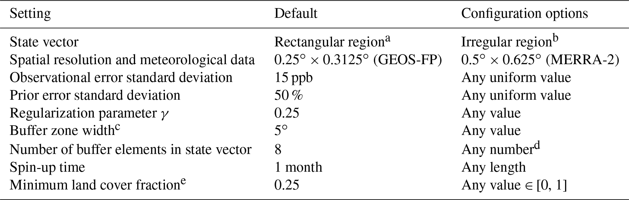
a Defined automatically from user-selected latitude and longitude bounds for the region of interest. b Either specified with a shapefile or defined by a pre-generated custom state vector file. c Extension of the inversion domain beyond the region of interest to absorb errors in boundary conditions. d Buffer elements are specified with a k-means algorithm. e Minimum land cover fraction for inclusion of a GEOS-Chem emission element in the state vector (see Sect. 2.3). Land cover information is from GEOS-FP or MERRA-2.
Workflow users begin by opening an EC2 instance and selecting the workflow AMI. The AMI contains the GEOS-Chem and IMI source codes, a configuration file, and all required software dependencies. They then specify a region and time period of interest in the configuration file. The configuration file also contains options to modify the IMI default settings (Table 2). Detailed instructions for configuring the IMI are provided in the online technical documentation (https://imi.seas.harvard.edu, last access: 8 June 2022). Users can use as prior estimates the default bottom-up emission inventories provided with the workflow (Table 1), or they can substitute their own. They can run the IMI preview (Fig. 3) to collect and visualize the TROPOMI and prior emission data for their selected region and time period and to get a rough estimate of information content and cost (Sect. 2.7). The preview incurs no significant computational cost. If the information content is deemed sufficient, the user can go on to run the IMI, including construction of the Jacobian matrix. This is the main computational cost but is very reasonable for typical inversion domains and periods (see Sect. 4.3 and Table 3). Once the Jacobian matrix has been constructed to define the forward model transport, it can be re-used to populate an inversion ensemble at no significant added computational cost by varying inversion parameters and/or bottom-up emission inventories (the latter requires rescaling the matrix). It can also be archived for later use.
The current IMI version 1.0 can be applied to any region of interest but has enhanced performance for regions within North America (10–70∘ N, 40–140∘ W), Europe (33–61∘ N, 30∘ W–70∘ E), and Asia (11∘ S–55∘ N, 60–150∘ E), where pre-cut continental subsets of the GEOS meteorological data (GEOS-FP and MERRA-2) are available to reduce computational cost. These subsets correspond to the default windows used in GEOS-Chem nested simulations (Kim et al., 2015; Zhang et al., 2015). The meteorological data for these three windows are uploaded to AWS by the GEOS-Chem support team with a latency of a few weeks. Users may apply the IMI to other regions using the full global GEOS meteorological data or after cropping the global data to a suitable nesting domain, following instructions and tools available on the IMI website (https://imi.seas.harvard.edu, last access: 11 July 2022). Future IMI versions will expand the pre-cut windows to other continents.
Figure 4 charts the IMI computational workflow as described in Sect. 2 and contained in the AMI. The workflow receives instructions from the configuration file and then has three basic steps: (i) perform an ensemble of GEOS-Chem simulations to define the transport features for individual emission state vector elements, (ii) use those simulations to construct the Jacobian matrix, and (iii) solve the analytical inversion using Eqs. (3)–(5). When the user configures and runs the IMI, these steps are executed automatically to generate posterior methane emission estimates for the inversion domain along with error statistics. The user can then inspect the inversion results using a visualization notebook provided with the IMI. The notebook contains sample code to plot the state vector, prior emissions, posterior emissions, scale factors (posterior and prior ratios), averaging kernel sensitivities, and TROPOMI data for the inversion domain and period.
The IMI workflow begins by constructing the emission state vector (length n) from the user specifications. After an initial spin-up simulation to generate initial conditions for the period of interest, it then performs n+1 GEOS-Chem simulations. These include a reference simulation driven by the prior bottom-up emission inventories and n perturbation simulations perturbing one emission element at a time. All of these simulations access S3 data for prior emissions, meteorology, and boundary conditions (Fig. 3). The perturbation simulations determine the sensitivities of the satellite observations to the state variables and are used to construct the Jacobian matrix K as described in Sect. 2.6. For our 1-month Permian Basin example (n=243), a total of 244 simulations are performed in this way. The reference and perturbation simulations are embarrassingly parallel and can be performed simultaneously once the spin-up simulation is complete if n+1 CPUs are available on the user's EC2 instance; with fewer CPUs the workflow runs the simulations in parallel batches.
After computing K from the reference and perturbation simulations, the IMI solves Eqs. (3)–(5) for the optimized emission estimates , posterior errors , and averaging kernel matrix A and saves these quantities as output. The elements of and the diagonal entries of A (averaging kernel sensitivities) and are then mapped to the grid cells of the inversion domain and saved as a separate output to facilitate inspection of the results, but archiving of the full matrices allows users to further inspect error correlations and smoothing. The final step of the workflow is to conduct a GEOS-Chem simulation using the posterior emissions for comparison to the TROPOMI observations and to a GEOS-Chem simulation using prior emissions (reference simulation) to verify the quality of the inversion results in better fitting the TROPOMI observations. This comparison could be performed more quickly by applying a correction to the prior forward model results, but running the full posterior simulation has the advantage of allowing validation against independent (e.g., ground-based) observations. Posterior simulation results are provided as part of the IMI output.
4.1 Setup
We perform a 1-month inversion for the Permian Basin (currently the most prolific US oil-producing basin) as an illustrative application of the IMI. We choose 1–31 May 2018 as the period of interest for the inversion. The region of interest is defined from a shapefile for the Permian Basin and comprises 235 state vector elements to describe emissions within the region at 0.25∘ × 0.3125∘ resolution, plus 8 buffer elements to pad out the inversion domain, for a total of 243 state vector elements (Fig. 1).
We perform the inversion using the default IMI settings laid out in Tables 1 and 2 but with the custom state vector of Fig. 1. The steps prior to initiating the inversion are as follows:
-
Create an AWS instance with the IMI workflow AMI.
-
Connect to the instance, upload the custom state vector file of Fig. 1, and open the configuration file.
-
Set the start date to 1 May 2018 and the end date to 1 June 2018.
-
Turn off the option to automatically generate the state vector from the latitude and longitude bounds of a rectangular region of interest.
-
Enter the path to the custom state vector file and close the configuration file.
-
Run the IMI preview to display the TROPOMI data and prior emissions, and estimate the information content to be achieved in the inversion.
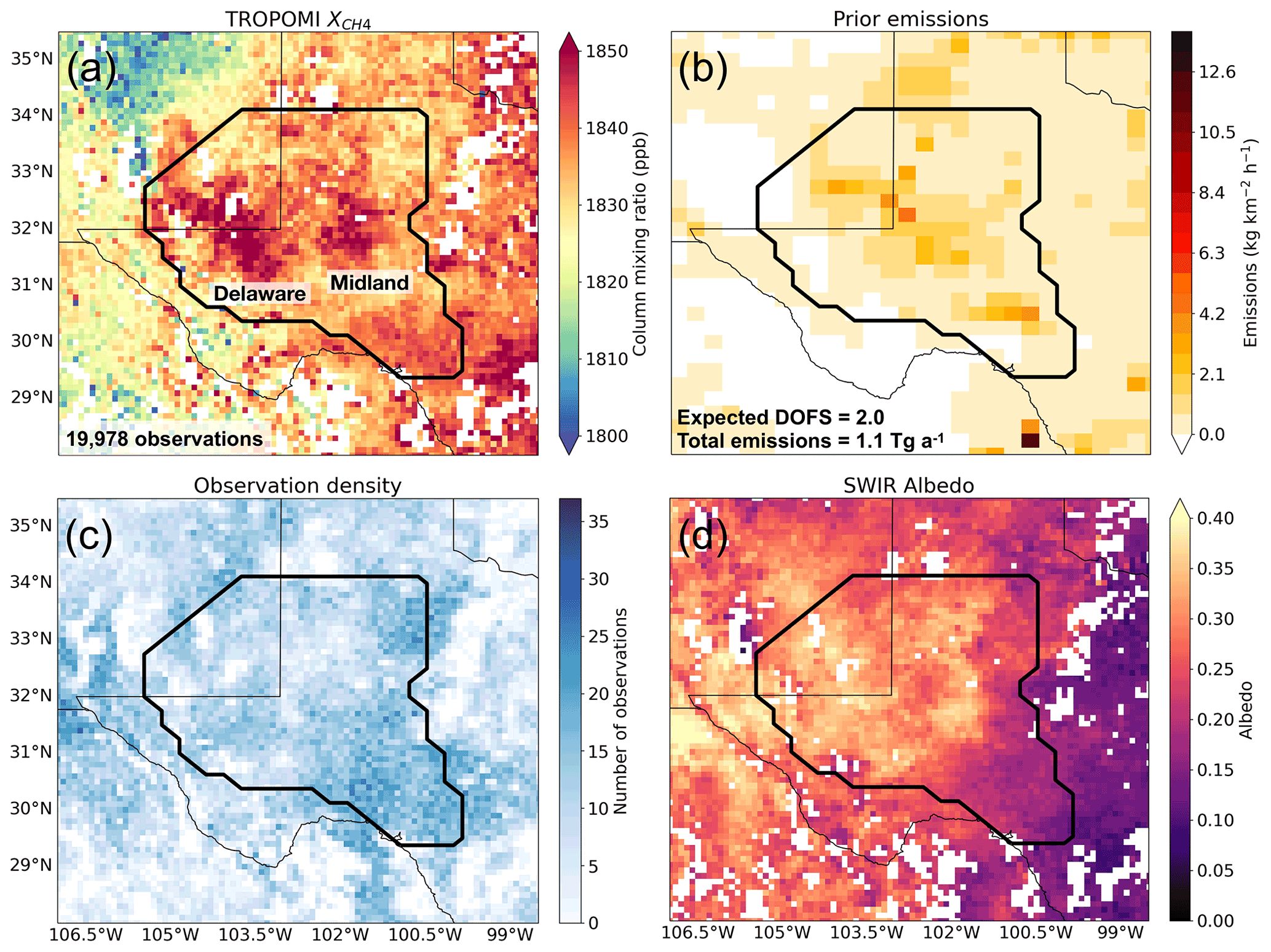
Figure 5Output of the IMI preview (Sect. 2.7) applied to the Permian Basin example with the default EPA gridded GHGI inventory (Maasakkers et al., 2016) as prior estimate of emissions. (a) Mean TROPOMI column-average dry-air methane mixing ratio () data for the user-selected region (thick black contour) and period of interest (1–31 May 2018), resampled to a 0.1∘ × 0.1∘ grid and cropped to 28–35.5∘ N, 98.5–107∘ W for visibility. The color bar is saturated to highlight methane hotspots over the Delaware and Midland sub-basins. Inset gives the total number of observations and degrees of freedom for signal (DOFS) for the region of interest. (b) Gridded GHGI (default) prior emissions. (c) Number of observations per 0.1∘ × 0.1∘ grid cell for the period of interest. (d) Mean SWIR albedo for the period of interest on the 0.1∘ × 0.1∘ grid. Here the preview shows poor agreement in the spatial distribution of emissions between the observations and prior emission estimates, suggesting that the prior estimate should be replaced by a better one (as is done in our application) or that the prior error estimate should be increased.
4.2 Analysis of results
Figure 5 shows the IMI preview results including the mean TROPOMI data for the selected region and period, the observation density, the TROPOMI SWIR albedo, and the default prior emission estimates (here the EPA GHGI). The TROPOMI data (Fig. 5a) include N = 19 978 individual observations for the region of interest, and these are used for the DOFS estimate in the preview. There are more than 100 000 additional observations in the inversion domain outside the region of interest and covering the buffer grid cells (Fig. 1). The two methane hotspots at the center of Fig. 5a correspond to the Permian's Delaware and Midland sub-basins. TROPOMI provides relatively uniform sampling across the region of interest (Fig. 5c), and visual comparison of Fig. 5a and d shows no indication of albedo-related regional biases. However, we see that the gridded GHGI inventory (Fig. 5b) severely misrepresents the spatial distribution of emissions in the Permian by failing to capture the sub-basin structure apparent in Fig. 5a. Furthermore, the inversion preview indicates an expected DOFS value of 2.0, which is marginal for quantifying emissions on that regional scale (Shen et al., 2021b).
At this point it would be sensible to reconfigure the IMI before performing the inversion, and we explain how to do so in what follows. If we proceed and conduct the inversion with these default settings, we find a DOFS of 1.9 (close to the preview). The posterior emission integrated over the region of interest is 1.8 Tg a−1, much higher than the default GHGI prior emission of 1.1 Tg a−1, and with scale factors (posterior over prior ratios) ranging from 1.0 to 3.3. These results are consistent with independent observations that the GHGI emissions for the Permian Basin are far too low (Omara et al., 2018; Robertson et al., 2020; Y. Chen et al., 2022; Cusworth et al., 2021b; Irakulis-Loitxate et al., 2021; Lyon et al., 2021), but the low DOFS and biased spatial distribution in the prior emissions do not inspire confidence in the results.
One can increase the DOFS simply by increasing the length of the inversion period, thus accumulating more observations, but the incorrect spatial distribution of the prior estimate will make it harder for the inversion to converge to the correct solution (Yu et al., 2021). An alternative is to increase the magnitude of the prior error estimate, but this may result in unphysical solutions if the problem is underconstrained in part of the domain. The user can judge from the output if these issues are severe.
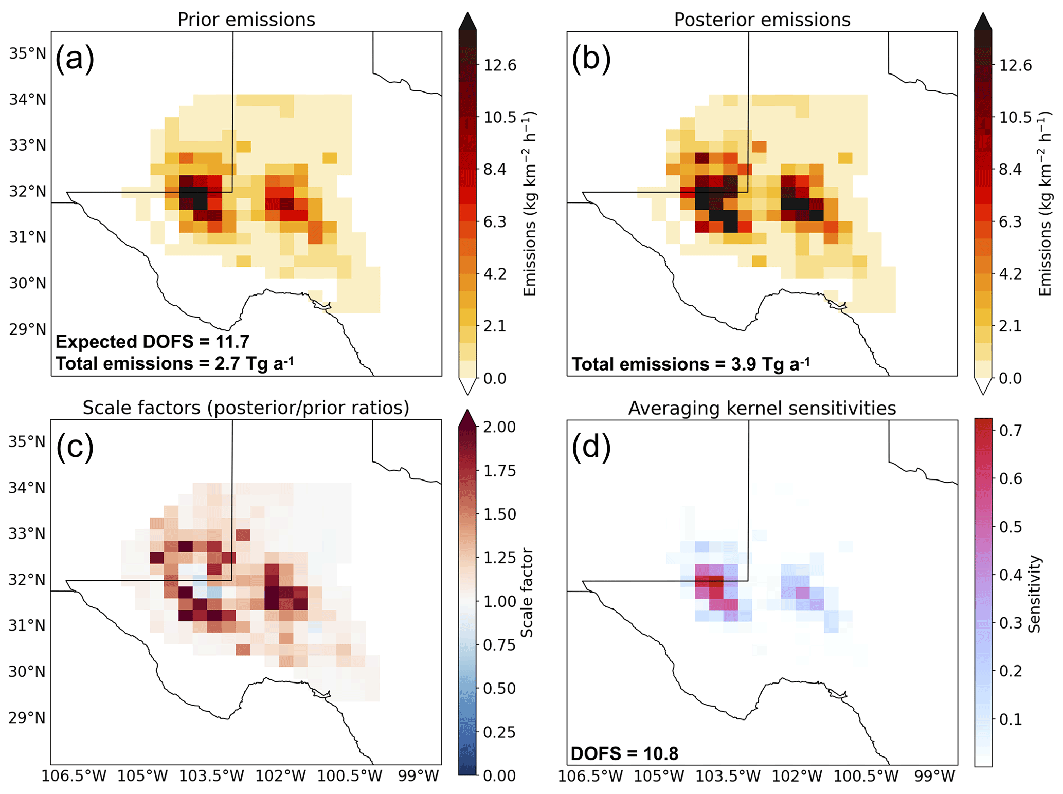
Figure 6Results of a 1-month (1–31 May 2018) application of the IMI to the Permian Basin using the EDF emission inventory (Zhang et al., 2020) as prior estimate of emissions. (a) Prior emissions. (b) Posterior emissions. (c) Scale factors applied to the prior emissions to obtain the posterior emissions. (d) Averaging kernel sensitivities with associated degrees of freedom for signal (DOFS) inset.
A better alternative is to investigate whether an improved bottom-up inventory would enable a more accurate inversion. In the case of the Permian Basin, an alternative gridded bottom-up inventory is available from the Environmental Defense Fund (EDF) with more accurate accounting of oil and gas infrastructure and larger total emissions of 2.7 Tg a−1 (Zhang et al., 2020). IMI results using the EDF inventory as a custom bottom-up prior estimate are shown in Fig. 6. Starting with the IMI preview, we find that the spatial distribution of prior emissions is much more consistent with the TROPOMI data (Fig. 6a, compare to Fig. 5b), with a much higher expected DOFS value of 11.7 that reflects the higher prior emissions (and hence the larger absolute prior error standard deviations). Proceeding to run the IMI workflow, we find that the posterior emissions now total 3.9 Tg a−1, up 45 % from the prior estimate of 2.7 Tg a−1 and with clear demarcation of the two sub-basins. The new scale factors range from 0.68 to 2.55, reflecting a need for both increased and decreased emissions in different parts of the basin to better match the satellite data. The averaging kernel sensitivities yield a DOFS value of 10.8 (consistent with the IMI preview), which gives us confidence in the inversion results both on the basin scale and in the spatial allocation within the basin. In particular, we see the need for more systematic increase in emissions in the Midland than the Delaware sub-basin.
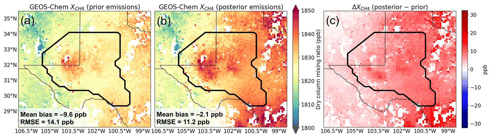
Figure 7GEOS-Chem simulations of TROPOMI observations for May 2018 with (a) prior emissions and (b) posterior emissions. Panel (c) shows the difference between the two. The contour line shows the Permian Basin selected as the region of interest for the inversion. The insets give the mean bias and RMSE for the region of interest in comparison to the TROPOMI observations in Fig. 5a.
Figure 7 shows the GEOS-Chem simulations for the inversion period with the prior and posterior emissions. The posterior simulation produces much higher methane concentrations over the Midland sub-basin, better matching the TROPOMI observations of Fig. 5. The mean GEOS-Chem-TROPOMI bias across the region of interest improves from −9.6 ppb in the reference simulation to −2.1 ppb in the posterior simulation, and the root mean square error (RMSE) improves from 14.1 to 11.2 ppb. A longer inversion would further decrease the bias and improve the RMSE.
Table 3Breakdown of IMI runtime by task for a 1-month Permian Basin inversion (May 2018)a.
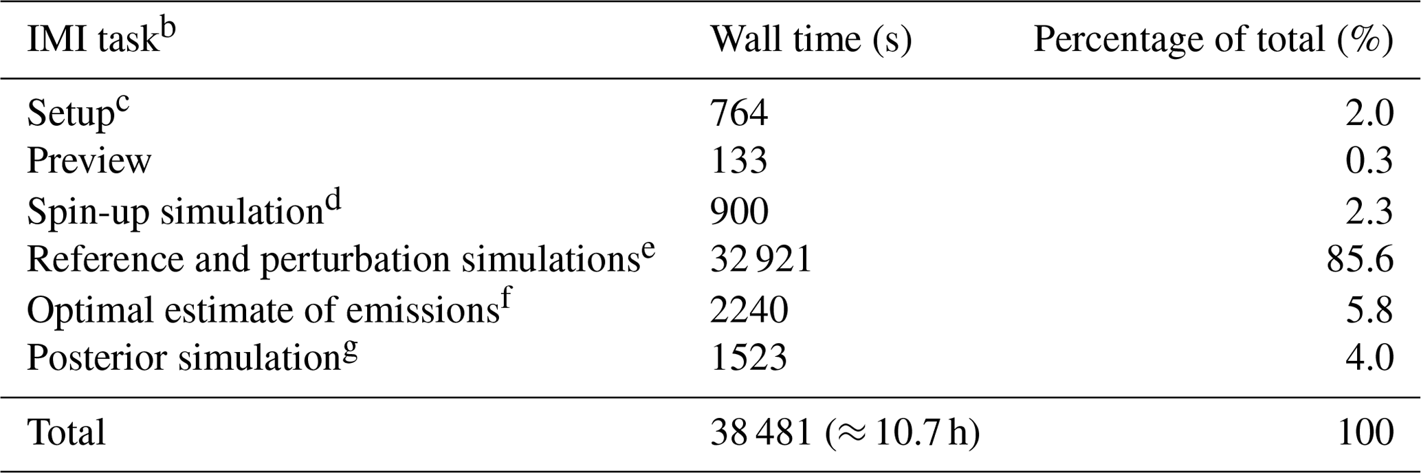
a Using an AWS EC2 c5.9xlarge instance with 36 CPUs and 500 GB of EBS storage. b See Sect. 3 for a detailed description of the tasks. c Includes compiling GEOS-Chem, preparing all GEOS-Chem run directories, and fetching input data from S3 (see Fig. 3). d Shared-memory parallelism (36 CPUs) for spin-up and posterior simulations grants ∼ 5–6× speed-up, limited by input and output. e Run in parallel batches with 1 CPU per simulation. f Solution to Eqs. (3)–(5). g Includes sampling of the GEOS-Chem atmosphere with the TROPOMI operator (see Fig. 2).
4.3 Cost
We conducted the illustrative inversion presented here on an AWS EC2 c5.9xlarge instance with 36 CPUs and 500 GB of EBS storage. Table 3 shows the runtime for different components of the IMI workflow. Compute wall time was 10.7 h, with > 85 % of that time spent constructing the Jacobian matrix K. Our cost was USD 17 for an “on-demand” instance, in which the requested resources are made available almost immediately. A 1-year inversion would cost roughly USD 300 (12 × USD 17 = USD 204, plus the cost of additional EBS storage to accommodate the longer inversion period), and wall time could be reduced by requesting more CPUs at no additional cost since the charge is per CPU hour. Costs scale linearly with the area of the inversion domain and (for a fixed domain size) the number of state vector elements, again subject to changes in EBS storage needs. Performing additional inversions with different parameters and prior inventories (Table 2, Sect. 4.2) adds little cost because there is no need to reconstruct K. Data download and transfer between AWS services may incur some cost, but this is also minimal. A cheaper alternative to on-demand instances are “spot instances”, which tap unused EC2 capacity and can reduce costs by a factor of 3–4 or more (Zhuang et al., 2019). Spot instances can be reclaimed by AWS at any time, which would cause the IMI to crash, but in practice this is rare, and users can generally expect to retain a spot instance for up to a month of wall time (Pary, 2018).
There is a growing demand for tools to infer regional methane emissions with high resolution from satellite data. Our Integrated Methane Inversion (IMI) workflow addresses this demand by enabling researchers and stakeholders to estimate methane emissions for regions of interest at 0.25∘ × 0.3125∘ (≈ 25 km × 25 km) resolution by Bayesian inversion of TROPOMI satellite observations on the AWS cloud, using cutting-edge inversion methodology and without requiring massive data download or advanced technical expertise. The workflow interfaces with TROPOMI operational data and the GEOS-Chem model already resident on AWS. It makes use of bottom-up emission inventories, GEOS-FP meteorological data, and boundary conditions (smoothed 3-D TROPOMI fields) that are also stored on AWS. There is no need for large TROPOMI data download. By automatically accessing all the needed resources on the cloud, the IMI embodies the new paradigm of “bringing compute to data” when working with very large datasets.
We outlined how users can configure and run the workflow to optimize methane emissions for a selected region and period of interest. The configuration can be as simple as defining the region (latitude–longitude bounds) and time period (start and end dates) or more complex for users wishing to customize different aspects of the inversion such as the state vector, the prior and observational errors, or the emission inventories used as prior estimates. The TROPOMI and GEOS-FP data are operationally uploaded to the AWS cloud with a latency of a few days so that continued access to current conditions is available.
The inversion uses an advanced research-grade algorithm to derive the best posterior estimates of emissions on the 0.25∘ × 0.3125∘ grid by analytical solution to a Bayesian cost function. The analytical solution provides closed-form error statistics on the posterior estimates and metrics on the information content from the observations including averaging kernel sensitivities and the degrees of freedom for signal (DOFS). It enables no-cost error analysis by producing an ensemble of solutions to explore the sensitivity to inversion parameters. The algorithm is fully documented in the literature (Turner et al., 2015; Maasakkers et al., 2019, 2021; Zhang et al., 2021; Lu et al., 2022), including applications to TROPOMI data (Zhang et al., 2020; Qu et al., 2021; Shen et al., 2021, 2022; Z. Chen et al., 2022). It is described in detail in the present paper, which can serve as a reference.
An IMI preview feature allows users to inspect the TROPOMI data and the anticipated quality of the inversion results for the region and period of interest before committing to the actual inversion. The IMI preview inspects the TROPOMI data for artifacts correlated with SWIR albedo, determines the observation density across the region of interest, gives a rough estimate of the DOFS to be expected from the inversion, and compares the spatial distribution of the prior estimates to the TROPOMI data. Large differences in spatial distributions may require adjustments to the prior estimates for a successful inversion.
We presented an illustrative application of the IMI workflow to a 1-month inversion of TROPOMI observations over the US Permian Basin. We showed how the DOFS and spatial distribution of prior emissions generated by the IMI preview allowed us to identify the limitations of the initially intended first inversion, which we fixed by swapping in an improved prior emission inventory. The subsequent inversion was performed at a cost less than USD 20 using an AWS c5.9xlarge “on-demand” instance with 36 CPUs, and could have been a factor of 3–4 cheaper using a “spot” instance.
This initial version of the IMI (version 1.0) has some limitations in functionality and does not include some of the newer capabilities recently developed within the analytical inversion framework. Priority developments for future IMI versions include (1) extension of pre-cut GEOS windows to continental domains outside of North America, Europe, and Asia; (2) the option to use lognormal rather than normal error pdf's for prior emissions to resolve the long tail of the emission distribution (Maasakkers et al., 2019; Z. Chen et al., 2022); (3) the option to use non-uniform prior and observational error covariance matrices, including off-diagonal terms; (4) upgrade of the global GEOS-Chem simulation used to generate boundary conditions from 4∘ × 5∘ to 2∘ × 2.5∘ resolution; (5) more optimal selection of state vector elements with a Gaussian mixture model (Turner and Jacob, 2015); (6) use of Kalman filter techniques for continuous emission monitoring with user-specified update frequency (Varon et al., 2022b); (7) incorporation of data from future globally surveying satellite instruments including GeoCarb (Moore et al., 2018), CO2M (Sierk et al., 2019), MethaneSAT (Wofsy and Hamburg, 2019), and GOSAT-GW (Kasahara et al., 2020); and (8) application to inversions for CO and CO2 emissions. This together with continued improvements to the operational TROPOMI methane product will make the IMI an increasingly powerful tool for researchers and stakeholders to monitor methane emissions worldwide at high resolution using satellite data.
Source code and documentation for the IMI are available at https://imi.seas.harvard.edu (last access: 18 July 2022; Varon et al., 2022a). The code used in this paper is permanently archived at https://doi.org/10.5281/zenodo.6578547 (Varon et al., 2022c).
The TROPOMI methane data are available on the Amazon Web Services (AWS) cloud at https://registry.opendata.aws/sentinel5p (last access: 8 June 2022; AWS, 2022). The GEOS-FP emission fields, boundary condition fields, and meteorological fields are available on AWS at https://registry.opendata.aws/geoschem-input-data (AWS, 8 June 2022).
DJV, MS, and DJJ contributed to the study conceptualization. DJV, MS, LAE, WBD, LS, and SEH developed the model code. DJV, DJJ, HN, ZQ, EP, ZC, XL, AL, AT, and CAR contributed to the methods' development. DJV performed the data analysis. DJV wrote the original draft, and all authors reviewed and edited the manuscript.
The contact author has declared that none of the authors has any competing interests.
Publisher's note: Copernicus Publications remains neutral with regard to jurisdictional claims in published maps and institutional affiliations.
This research has been supported by the National Aeronautics and Space Administration (NASA; Carbon Monitoring System; grant no. 80NSSC21K1057) and the ExxonMobil Research and Engineering Company (PO number 620 / 4520099721).
This paper was edited by Fiona O'Connor and reviewed by Christian Frankenberg and one anonymous referee.
AWS: Sentinel-5P Level 2, aws [data set], https://registry.opendata.aws/sentinel5p, last access: 8 June 2022.
AWS: GEOS-Chem Input Data, AWS [data set], https://registry.opendata.aws/geoschem-input-data, last access: 8 June 2022.
Barré, J., Aben, I., Agustí-Panareda, A., Balsamo, G., Bousserez, N., Dueben, P., Engelen, R., Inness, A., Lorente, A., McNorton, J., Peuch, V.-H., Radnoti, G., and Ribas, R.: Systematic detection of local CH4 anomalies by combining satellite measurements with high-resolution forecasts, Atmos. Chem. Phys., 21, 5117–5136, https://doi.org/10.5194/acp-21-5117-2021, 2021.
Bergamaschi, P., Houweling, S., Segers, A., Krol, M., Frankenberg, C., Scheepmaker, R. A., Dlugokencky, E., Wofsy, S. C., Kort, E. A., Sweeney, C., Schuck, T., Brenninkmeijer, C., Chen, H., Beck, V., and Gerbig, C.: Atmospheric CH4 in the first decade of the 21st century: Inverse modeling analysis using SCIAMACHY satellite retrievals and NOAA surface measurements, J. Geophys. Res.-Atmos., 118, 7350–7369, https://doi.org/10.1002/jgrd.50480, 2013.
Bloom, A. A., Bowman, K. W., Lee, M., Turner, A. J., Schroeder, R., Worden, J. R., Weidner, R., McDonald, K. C., and Jacob, D. J.: A global wetland methane emissions and uncertainty dataset for atmospheric chemical transport models (WetCHARTs version 1.0), Geosci. Model Dev., 10, 2141–2156, https://doi.org/10.5194/gmd-10-2141-2017, 2017.
Brasseur, G. P. and Jacob, D. J.: Modeling of Atmospheric Chemistry, Cambridge University Press, Cambridge, UK, 2017.
Buchwitz, M., Reuter, M., Schneising, O., Boesch, H., Guerlet, S., Dils, B., Aben, I., Armante, R., Bergamaschi, P., Blumenstock, T., Bovensmann, H., Brunner, D., Buchmann, B., Burrows, J. P., Butz, A., Chédin, A., Chevallier, F., Crevoisier, C. D., Deutscher, N. M., Frankenberg, C., Hase, F., Hasekamp, O. P., Heymann, J., Kaminski, T., Laeng, A., Lichtenberg, G., De Mazière, M., Noël, S., Notholt, J., Orphal, J., Popp, C., Parker, R., Scholze, M., Sussmann, R., Stiller, G. P., Warneke, T., Zehner, C., Bril, A., Crisp, D., Griffith, D. W. T., Kuze, A., O'Dell, C., Oshchepkov, S., Sherlock, V., Suto, H., Wennberg, P., Wunch, D., Yokota, T., and Yoshida, Y.: The Greenhouse Gas Climate Change Initiative (GHG-CCI): Comparison and quality assessment of near-surface-sensitive satellite-derived CO2 and CH4 global data sets, Remote Sens. Environ., 162, 344–362, https://doi.org/10.1016/j.rse.2013.04.024, 2015.
Butz, A., Hasekamp, O., Frankenberg, C., and Aben, I.: Retrievals of atmospheric CO2 from simulated space-borne measurements of backscattered near-infrared sunlight: accounting for aerosol effects, Appl. Optics, 48, 3322, https://doi.org/10.1364/AO.48.003322, 2009.
Butz, A., Hasekamp, O., Frankenberg, C., Vidot, J., and Aben, I.: CH4 retrievals from spacebased solar backscatter measurements: performance evaluation against simulated aerosol and cirrus loaded scenes, J. Geophys. Res., 115, D24302, https://doi.org/10.1029/2010JD014514, 2010.
Butz, A., Guerlet, S., Hasekamp, O., Schepers, D., Galli, A., Aben, I., Frankenberg, C., Hartmann, J. M., Tran, H., Kuze, A., Keppel-Aleks, G., Toon, G., Wunch, D., Wennberg, P., Deutscher, N., Griffith, D., Macatangay, R., Messerschmidt, J., Notholt, J., and Warneke, T.: Toward accurate CO2 and CH4 observations from GOSAT, Geophys. Res. Lett., 38, L14812, https://doi.org/10.1029/2011GL047888, 2011.
Butz, A., Galli, A., Hasekamp, O., Landgraf, J., Tol, P., and Aben, I.: TROPOMI aboard Sentinel-5 Precursor: Prospective performance of CH4 retrievals for aerosol and cirrus loaded atmospheres, Remote Sens. Environ., 120, 267–276, 2012.
Chen, Y., Sherwin, E. D., Berman, E. S. F., Jones, B. B., Gordon, M. P., Wetherley, E. B., Kort, E. A., and Brandt, A. R.: Quantifying Regional Methane Emissions in the New Mexico Permian Basin with a Comprehensive Aerial Survey, Environ. Sci. Technol., 56, 4317–4323, https://doi.org/10.1021/acs.est.1c06458, 2022.
Chen, Y.-H. and Prinn, R. G.: Estimation of atmospheric methane emissions between 1996 and 2001 using a three-dimensional global chemical transport model, J. Geophys. Res., 111, D10307, https://doi.org/10.1029/2005JD006058, 2006.
Chen, Z., Jacob, D., Nesser, H., Sulprizio, M., Lorente, A., Varon, D., Lu, X., Shen, L., Qu, Z., Penn, E., and Yu, X.: Methane emissions from China: a high-resolution inversion of TROPOMI satellite observations, Atmos. Chem. Phys. Discuss. [preprint], https://doi.org/10.5194/acp-2022-303, in review, 2022.
Cui, T., Martin, J., Marzouk, Y. M., Solonen, A., and Spantini, A.: Likelihood-informed dimension reduction for nonlinear inverse problems, Inverse Probl., 30, 114015, https://doi.org/10.1088/0266-5611/30/11/114015, 2014.
Cusworth, D. H., Bloom, A. A., Ma, S., Miller, C. E., Bowman, K., Yin, Y., Maasakkers, J. D., Zhang, Y., Scarpelli, T. R., Qu, Z., Jacob, D. J., and Worden, J. R.: A Bayesian framework for deriving sector-based methane emissions from top-down fluxes, Commun. Earth Environ., 2, 242, https://doi.org/10.1038/s43247-021-00312-6, 2021a.
Cusworth, D. H., Duren, R. M., Thorpe, A. K., Olson-Duvall, W., Heckler, J., Chapman, J. W., Eastwood, M. L., Helmlinger, M. C., Green, R. O., Asner, G. P., Dennison, P. E., and Miller, C. E.: Intermittency of large methane emitters in the Permian Basin, Environ. Sci. Tech. Let., 8, 567–573, https://doi.org/10.1021/acs.estlett.1c00173, 2021b.
de Gouw, J. A., Veefkind, J. P., Roosenbrand, E., Dix, B., Lin, J. C., Landgraf, J., and Levelt, P. F.: Daily Satellite Observations of Methane from Oil and Gas Production Regions in the United States, Sci. Rep., 10, 1379, https://doi.org/10.1038/s41598-020-57678-4, 2020.
EC and USA: Global Methane Pledge, European Commission and United States of America, https://www.ccacoalition.org/en/resources/global-methane-pledge (last access: 8 June 2022), 2021.
ECCC: National Inventory Report 1990-2018: Greenhouse Gas Sources and Sinks in Canada, Environment and Climate Change Canada (ECCC), Gatineau, QC, http://publications.gc.ca/pub?id=9.506002&sl=0 (last access: October 2020), 2020.
EPA: Inventory of US Greenhouse Gas Emissions and Sinks: 1990–2014, the U.S. Environmental Protection Agency, https://www.epa.gov/ghgemissions/us-greenhouse-gas-inventory-report-1990-2014 (last access: 18 July 2022), 2016.
Etiope, G., Ciotoli, G., Schwietzke, S., and Schoell, M.: Gridded maps of geological methane emissions and their isotopic signature, Earth Syst. Sci. Data, 11, 1–22, https://doi.org/10.5194/essd-11-1-2019, 2019.
Fung, I., John, J., Lerner, J., Matthews, E., Prather, M., Steele, L. P., and Fraser, P. J.: Three-dimensional model synthesis of the global methane cycle, J. Geophys. Res.-Atmos., 96, 13033–13065, https://doi.org/10.1029/91JD01247, 1991.
Hachmeister, J., Schneising, O., Buchwitz, M., Lorente, A., Borsdorff, T., Burrows, J. P., Notholt, J., and Buschmann, M.: On the influence of underlying elevation data on Sentinel-5 Precursor TROPOMI satellite methane retrievals over Greenland, Atmos. Meas. Tech., 15, 4063–4074, https://doi.org/10.5194/amt-15-4063-2022, 2022.
Hansen, P. C.: The L-curve and its use in the numerical treatment of inverse problems, IMM Tech. Rep. 15/1999, Kongens Lyngby, Denmark, 1999.
Hasekamp, O., Lorente, A., Hu, H., Butz, A., aan de Brugh, J., and Landgraf, J.: Algorithm Theoretical Baseline Document for Sentinel-5 Precursor Methane Retrieval, Sron-S5P-Lev2-Rp-001, (v1.10), European Space Agency technical document, 1–67, European Space Agency, https://sentinel.esa.int/documents/247904/2476257/Sentinel-5P-TROPOMI-ATBD-Methane-retrieval (last access: 23 November 2021), 2019.
Hmiel, B., Petrenko, V. V., Dyonisius, M. N., Buizert, C., Smith, A. M., Place, P. F., Harth, C., Beaudette, R., Hua, Q., Yang, B., Vimont, I., Michel, S. E., Severinghaus, J. P., Etheridge, D., Bromley, T., Schmitt, J., Faïn, X., Weiss, R. F., and Dlugokencky, E.: Preindustrial 14CH4 indicates greater anthropogenic fossil CH4 emissions, Nature, 578, 409–412, https://doi.org/10.1038/s41586-020-1991-8, 2020.
Hu, H., Hasekamp, O., Butz, A., Galli, A., Landgraf, J., Aan de Brugh, J., Borsdorff, T., Scheepmaker, R., and Aben, I.: The operational methane retrieval algorithm for TROPOMI, Atmos. Meas. Tech., 9, 5423–5440, https://doi.org/10.5194/amt-9-5423-2016, 2016.
Hu, H., Landgraf, J., Detmers, R., Borsdorff, T., Aan de Brugh, J., Aben, I., Butz, A., and Hasekamp, O.: Toward global mapping of methane with TROPOMI: First results and intersatellite comparison to GOSAT, Geophys. Res. Lett., 45, 3682–3689, https://doi.org/10.1002/2018GL077259, 2018.
INECC and SEMARNAT: Sexta Comunicación Nacional y Segundo Informe Bienal de Actualización ante la Convención Marco de las Naciones Unidas sobre el Cambio Climático, Instituto Nacional de Ecología y Cambio Climático (INECC) and Secretaría de Medio Ambiente y Recursos Naturales (SEMARNAT), México, 2018.
IPCC: 2019 Refinement to the 2006 IPCC Guidelines for National Greenhouse Gas Inventories, edited by: Calvo Buendia, E., Tanabe, K., Kranjc, A., Jamsranjav, B., Fukuda, M., Ngarize, S., Osako, A., Pyrozhenko, Y., Shermanau, P., and Federici, S., IPCC, Switzerland, 2019.
Irakulis-Loitxate, I., Guanter, L., Liu, Y. N., Varon, D. J., Maasakkers, J. D., Zhang, Y., Chulakadabba, A., Wofsy, S. C., Thorpe, A. K., Duren, R. M., Frankenberg, C., Lyon, D. R., Hmiel, B., Cusworth, D. H., Zhang, Y., Segl, K., Gorroño, J., Sánchez-García, E., Sulprizio, M. P., Cao, K., Zhu, H., Liang, J., Li, X., Aben, I., and Jacob, D. J.: Satellite-based survey of extreme methane emissions in the Permian basin, Sci. Adv., 7, https://doi.org/10.1126/sciadv.abf4507, 2021.
Jacob, D. J., Turner, A. J., Maasakkers, J. D., Sheng, J., Sun, K., Liu, X., Chance, K., Aben, I., McKeever, J., and Frankenberg, C.: Satellite observations of atmospheric methane and their value for quantifying methane emissions, Atmos. Chem. Phys., 16, 14371–14396, https://doi.org/10.5194/acp-16-14371-2016, 2016.
Janssens-Maenhout, G., Crippa, M., Guizzardi, D., Muntean, M., Schaaf, E., Dentener, F., Bergamaschi, P., Pagliari, V., Olivier, J. G. J., Peters, J. A. H. W., van Aardenne, J. A., Monni, S., Doering, U., Petrescu, A. M. R., Solazzo, E., and Oreggioni, G. D.: EDGAR v4.3.2 Global Atlas of the three major greenhouse gas emissions for the period 1970–2012, Earth Syst. Sci. Data, 11, 959–1002, https://doi.org/10.5194/essd-11-959-2019, 2019.
Kasahara, M., Kachi, M., Inaoka, K., Fujii, H., Kubota, T., Shimada, R., and Kojima, Y.: Overview and current status of GOSAT-GW mission and AMSR3 instrument, in: Proc. SPIE 11530, Sensors, Systems, and Next-Generation Satellites XXIV, 1153007 (20 September 2020), https://doi.org/10.1117/12.2573914, 2020.
Kim, P. S., Jacob, D. J., Fisher, J. A., Travis, K., Yu, K., Zhu, L., Yantosca, R. M., Sulprizio, M. P., Jimenez, J. L., Campuzano-Jost, P., Froyd, K. D., Liao, J., Hair, J. W., Fenn, M. A., Butler, C. F., Wagner, N. L., Gordon, T. D., Welti, A., Wennberg, P. O., Crounse, J. D., St. Clair, J. M., Teng, A. P., Millet, D. B., Schwarz, J. P., Markovic, M. Z., and Perring, A. E.: Sources, seasonality, and trends of southeast US aerosol: an integrated analysis of surface, aircraft, and satellite observations with the GEOS-Chem chemical transport model, Atmos. Chem. Phys., 15, 10411–10433, https://doi.org/10.5194/acp-15-10411-2015, 2015.
Lin, H., Jacob, D. J., Lundgren, E. W., Sulprizio, M. P., Keller, C. A., Fritz, T. M., Eastham, S. D., Emmons, L. K., Campbell, P. C., Baker, B., Saylor, R. D., and Montuoro, R.: Harmonized Emissions Component (HEMCO) 3.0 as a versatile emissions component for atmospheric models: application in the GEOS-Chem, NASA GEOS, WRF-GC, CESM2, NOAA GEFS-Aerosol, and NOAA UFS models, Geosci. Model Dev., 14, 5487–5506, https://doi.org/10.5194/gmd-14-5487-2021, 2021.
Lorente, A., Borsdorff, T., Butz, A., Hasekamp, O., aan de Brugh, J., Schneider, A., Wu, L., Hase, F., Kivi, R., Wunch, D., Pollard, D. F., Shiomi, K., Deutscher, N. M., Velazco, V. A., Roehl, C. M., Wennberg, P. O., Warneke, T., and Landgraf, J.: Methane retrieved from TROPOMI: improvement of the data product and validation of the first 2 years of measurements, Atmos. Meas. Tech., 14, 665–684, https://doi.org/10.5194/amt-14-665-2021, 2021.
Lu, X., Jacob, D. J., Zhang, Y., Maasakkers, J. D., Sulprizio, M. P., Shen, L., Qu, Z., Scarpelli, T. R., Nesser, H., Yantosca, R. M., Sheng, J., Andrews, A., Parker, R. J., Boesch, H., Bloom, A. A., and Ma, S.: Global methane budget and trend, 2010–2017: complementarity of inverse analyses using in situ (GLOBALVIEWplus CH4 ObsPack) and satellite (GOSAT) observations, Atmos. Chem. Phys., 21, 4637–4657, https://doi.org/10.5194/acp-21-4637-2021, 2021.
Lu, X., Jacob, D. J., Wang, H., Maasakkers, J. D., Zhang, Y., Scarpelli, T. R., Shen, L., Qu, Z., Sulprizio, M. P., Nesser, H., Bloom, A. A., Ma, S., Worden, J. R., Fan, S., Parker, R. J., Boesch, H., Gautam, R., Gordon, D., Moran, M. D., Reuland, F., Villasana, C. A. O., and Andrews, A.: Methane emissions in the United States, Canada, and Mexico: evaluation of national methane emission inventories and 2010–2017 sectoral trends by inverse analysis of in situ (GLOBALVIEWplus CH4 ObsPack) and satellite (GOSAT) atmospheric observations, Atmos. Chem. Phys., 22, 395–418, https://doi.org/10.5194/acp-22-395-2022, 2022.
Lyon, D. R., Hmiel, B., Gautam, R., Omara, M., Roberts, K. A., Barkley, Z. R., Davis, K. J., Miles, N. L., Monteiro, V. C., Richardson, S. J., Conley, S., Smith, M. L., Jacob, D. J., Shen, L., Varon, D. J., Deng, A., Rudelis, X., Sharma, N., Story, K. T., Brandt, A. R., Kang, M., Kort, E. A., Marchese, A. J., and Hamburg, S. P.: Concurrent variation in oil and gas methane emissions and oil price during the COVID-19 pandemic, Atmos. Chem. Phys., 21, 6605–6626, https://doi.org/10.5194/acp-21-6605-2021, 2021.
Maasakkers, J. D., Jacob, D. J., Sulprizio, M. P., Turner, A. J., Weitz, M., Wirth, T., Hight, C., DeFigueiredo, M., Desai, M., and Schmeltz, R.: Gridded national inventory of US methane emissions, Environ. Sci. Technol., 50, 13123–13133, 2016.
Maasakkers, J. D., Jacob, D. J., Sulprizio, M. P., Scarpelli, T. R., Nesser, H., Sheng, J.-X., Zhang, Y., Hersher, M., Bloom, A. A., Bowman, K. W., Worden, J. R., Janssens-Maenhout, G., and Parker, R. J.: Global distribution of methane emissions, emission trends, and OH concentrations and trends inferred from an inversion of GOSAT satellite data for 2010–2015, Atmos. Chem. Phys., 19, 7859–7881, https://doi.org/10.5194/acp-19-7859-2019, 2019.
Maasakkers, J. D., Jacob, D. J., Sulprizio, M. P., Scarpelli, T. R., Nesser, H., Sheng, J., Zhang, Y., Lu, X., Bloom, A. A., Bowman, K. W., Worden, J. R., and Parker, R. J.: 2010–2015 North American methane emissions, sectoral contributions, and trends: a high-resolution inversion of GOSAT observations of atmospheric methane, Atmos. Chem. Phys., 21, 4339–4356, https://doi.org/10.5194/acp-21-4339-2021, 2021.
Miller, S. M., Michalak, A. M., Detmers, R. G., Hasekamp, O. P., Bruhwiler, L. M. P., and Schwietzke, S.: China's coal mine methane regulations have not curbed growing emissions, Nat. Commun., 10, 303, https://doi.org/10.1038/s41467-018-07891-7, 865, 2019.
Moore, B., Crowell, S. M. R., Rayner, P. J., Kumer, J., O'Dell, C. W., O'Brien, D., Utembe, S., Polonsky, I., Schimel, D., and Lemen, J.: The Potential of the Geostationary Carbon Cycle Observatory (GeoCarb) to Provide Multi-scale Constraints on the Carbon Cycle in the Americas, Front. Environ. Sci., 6, https://doi.org/10.3389/fenvs.2018.00109, 2018.
Murguia-Flores, F., Arndt, S., Ganesan, A. L., Murray-Tortarolo, G., and Hornibrook, E. R. C.: Soil Methanotrophy Model (MeMo v1.0): a process-based model to quantify global uptake of atmospheric methane by soil, Geosci. Model Dev., 11, 2009–2032, https://doi.org/10.5194/gmd-11-2009-2018, 2018.
Nesser, H., Jacob, D. J., Maasakkers, J. D., Scarpelli, T. R., Sulprizio, M. P., Zhang, Y., and Rycroft, C. H.: Reduced-cost construction of Jacobian matrices for high-resolution inversions of satellite observations of atmospheric composition, Atmos. Meas. Tech., 14, 5521–5534, https://doi.org/10.5194/amt-14-5521-2021, 2021.
Omara, M., Zimmerman, N., Sullivan, M. R., Li, X., Ellis, A., Cesa, R., Subramanian, R., Presto, A. A., and Robinson, A. L.: Methane Emissions from Natural Gas Production Sites in the United States: Data Synthesis and National Estimate, Environ. Sci. Technol., 52, 12915–12925, 2018.
Pary, R.: New Amazon EC2 Spot pricing model: Simplified purchasing without bidding and fewer interruptions, AWS Compute Blog, 13 March, https://aws.amazon.com/blogs/compute/new-amazon-ec2-spot-pricing/ (last accessed: 23 November 2021), 2018.
Qu, Z., Jacob, D. J., Shen, L., Lu, X., Zhang, Y., Scarpelli, T. R., Nesser, H., Sulprizio, M. P., Maasakkers, J. D., Bloom, A. A., Worden, J. R., Parker, R. J., and Delgado, A. L.: Global distribution of methane emissions: a comparative inverse analysis of observations from the TROPOMI and GOSAT satellite instruments, Atmos. Chem. Phys., 21, 14159–14175, https://doi.org/10.5194/acp-21-14159-2021, 2021.
Randerson, J. T., van der Werf, G. R., Giglio, L., Collatz, G. J., and Kasibhatla, P. S.: Global Fire Emissions Database, Version 4.1 (GFEDv4), ORNL DAAC, Oak Ridge, Tennessee, USA, https://doi.org/10.3334/ORNLDAAC/1293, 2018.
Robertson, A., Edie, R., Field, R. A., Lyon, D. R., McVay, R., Omara, M., Zavala-Araiza, D., and Murphy, S. M.: New Mexico Permian Basin Well Pad Methane Emissions are a Factor of 6–13 Times Higher Than US EPA Estimates, Environ. Sci. Technol., 54, 13926–13934, https://doi.org/10.1021/acs.est.0c02927, 2020.
Rodgers, C. D.: Inverse Methods for Atmospheric Sounding: Theory and Practice, World Scientific, River Edge, USA, 2000.
Saunois, M., Stavert, A. R., Poulter, B., Bousquet, P., Canadell, J. G., Jackson, R. B., Raymond, P. A., Dlugokencky, E. J., Houweling, S., Patra, P. K., Ciais, P., Arora, V. K., Bastviken, D., Bergamaschi, P., Blake, D. R., Brailsford, G., Bruhwiler, L., Carlson, K. M., Carrol, M., Castaldi, S., Chandra, N., Crevoisier, C., Crill, P. M., Covey, K., Curry, C. L., Etiope, G., Frankenberg, C., Gedney, N., Hegglin, M. I., Höglund-Isaksson, L., Hugelius, G., Ishizawa, M., Ito, A., Janssens-Maenhout, G., Jensen, K. M., Joos, F., Kleinen, T., Krummel, P. B., Langenfelds, R. L., Laruelle, G. G., Liu, L., Machida, T., Maksyutov, S., McDonald, K. C., McNorton, J., Miller, P. A., Melton, J. R., Morino, I., Müller, J., Murguia-Flores, F., Naik, V., Niwa, Y., Noce, S., O'Doherty, S., Parker, R. J., Peng, C., Peng, S., Peters, G. P., Prigent, C., Prinn, R., Ramonet, M., Regnier, P., Riley, W. J., Rosentreter, J. A., Segers, A., Simpson, I. J., Shi, H., Smith, S. J., Steele, L. P., Thornton, B. F., Tian, H., Tohjima, Y., Tubiello, F. N., Tsuruta, A., Viovy, N., Voulgarakis, A., Weber, T. S., van Weele, M., van der Werf, G. R., Weiss, R. F., Worthy, D., Wunch, D., Yin, Y., Yoshida, Y., Zhang, W., Zhang, Z., Zhao, Y., Zheng, B., Zhu, Q., Zhu, Q., and Zhuang, Q.: The Global Methane Budget 2000–2017, Earth Syst. Sci. Data, 12, 1561–1623, https://doi.org/10.5194/essd-12-1561-2020, 2020.
Scarpelli, T. R., Jacob, D. J., Octaviano Villasana, C. A., Ramirez Hernandez, I. F., Cardenas Moreno, P. R., Cortes Alfaro, E. A., Garcia Garcia, M. A., and Zavala-Araiza, D.: A gridded inventory of anthropogenic methane emissions from Mexico based on Mexico's National Inventory of Greenhouse Gases and Compounds, Environ. Res. Lett., 15, 105015, https://doi.org/10.7910/DVN/5FUTWM, 2020.
Scarpelli, T. R., Jacob, D. J., Moran, M., Reuland, F., and Gordon, D.: A gridded inventory of Canada's anthropogenic methane emissions, Environ. Res. Lett., 17, 014007, https://doi.org/10.1088/1748-9326/ac40b1, 2022a.
Scarpelli, T. R., Jacob, D. J., Grossman, S., Lu, X., Qu, Z., Sulprizio, M. P., Zhang, Y., Reuland, F., Gordon, D., and Worden, J. R.: Updated Global Fuel Exploitation Inventory (GFEI) for methane emissions from the oil, gas, and coal sectors: evaluation with inversions of atmospheric methane observations, Atmos. Chem. Phys., 22, 3235–3249, https://doi.org/10.5194/acp-22-3235-2022, 2022b.
Schneising, O., Buchwitz, M., Reuter, M., Bovensmann, H., Burrows, J. P., Borsdorff, T., Deutscher, N. M., Feist, D. G., Griffith, D. W. T., Hase, F., Hermans, C., Iraci, L. T., Kivi, R., Landgraf, J., Morino, I., Notholt, J., Petri, C., Pollard, D. F., Roche, S., Shiomi, K., Strong, K., Sussmann, R., Velazco, V. A., Warneke, T., and Wunch, D.: A scientific algorithm to simultaneously retrieve carbon monoxide and methane from TROPOMI onboard Sentinel-5 Precursor, Atmos. Meas. Tech., 12, 6771–6802, https://doi.org/10.5194/amt-12-6771-2019, 2019.
Shen, L., Zavala-Araiza, D., Gautam, R., Omara, M., Scarpelli, T., Sheng, J., Sulprizio, M. P., Zhuang, J., Zhang, Y., Lu, X., Hamburg, S. P., and Jacob, D. J.: Unravelling a large methane emission discrepancy in Mexico using satellite observations, Remote Sens. Environ., 260, 112461, https://doi.org/10.1016/j.rse.2021.112461, 2021.
Shen, L., Gautam, R., Omara, M., Zavala-Araiza, D., Maasakkers, J., Scarpelli, T., Lorente, A., Lyon, D., Sheng, J., Varon, D., Nesser, H., Qu, Z., Lu, X., Sulprizio, M., Hamburg, S., and Jacob, D.: Satellite quantification of oil and natural gas methane emissions in the US and Canada including contributions from individual basins, Atmos. Chem. Phys. Discuss. [preprint], https://doi.org/10.5194/acp-2022-155, in review, 2022.
Sierk, B., Bézy, J.-L., Löscher, A., and Meijer, Y.: The European CO2 Monitoring Mission: observing anthropogenic greenhouse gas emissions from space, in: Proc. SPIE 11180, International Conference on Space Optics – ICSO 2018, 111800M (12 July 2019), Chania, Greece, https://doi.org/10.1117/12.2535941, 2019.
Stanevich, I., Jones, D. B. A., Strong, K., Parker, R. J., Boesch, H., Wunch, D., Notholt, J., Petri, C., Warneke, T., Sussmann, R., Schneider, M., Hase, F., Kivi, R., Deutscher, N. M., Velazco, V. A., Walker, K. A., and Deng, F.: Characterizing model errors in chemical transport modeling of methane: impact of model resolution in versions v9-02 of GEOS-Chem and v35j of its adjoint model, Geosci. Model Dev., 13, 3839–3862, https://doi.org/10.5194/gmd-13-3839-2020, 2020.
Turner, A. J. and Jacob, D. J.: Balancing aggregation and smoothing errors in inverse models, Atmos. Chem. Phys., 15, 7039–7048, https://doi.org/10.5194/acp-15-7039-2015, 2015.
Turner, A. J., Jacob, D. J., Wecht, K. J., Maasakkers, J. D., Lundgren, E., Andrews, A. E., Biraud, S. C., Boesch, H., Bowman, K. W., Deutscher, N. M., Dubey, M. K., Griffith, D. W. T., Hase, F., Kuze, A., Notholt, J., Ohyama, H., Parker, R., Payne, V. H., Sussmann, R., Sweeney, C., Velazco, V. A., Warneke, T., Wennberg, P. O., and Wunch, D.: Estimating global and North American methane emissions with high spatial resolution using GOSAT satellite data, Atmos. Chem. Phys., 15, 7049–7069, https://doi.org/10.5194/acp-15-7049-2015, 2015.
Varon, D. J., Estrada, L. A., Sulprizio, M., and Jacob, D. J.: Integrated Methane Inversion Website, IMI [code], https://imi.seas.harvard.edu/ (last access: 18 July 2022), 2022a.
Varon, D. J., Jacob, D. J., Sulprizio, M. P., Shen, L., Qu, Z., Nesser, H., Gautam, R., Omara, M., Hmiel, B., Lyon, D., Delgado, A. L., Maasakkers, J., and Aben, I.: Continuous weekly monitoring of methane emissions from the Permian Basin by inversion of TROPOMI satellite observations (2A.2), American Meteorological Society 102nd annual meeting, 24 January 2022, Houston, Texas, January 2022b.
Varon, D. J., Laestrada, W. D., and Jiawei, Z.: geoschem/integrated_methane_inversion: imi 1.0.0-beta.2 release (imi-1.0.0-beta.2), Zenodo [code], https://doi.org/10.5281/zenodo.6578547, 2022c.
Wecht, K. J., Jacob, D. J., Frankenberg, C., Jiang, Z., and Blake, D. R.: Mapping of North America methane emissions with high spatial resolution by inversion of SCIAMACHY satellite data, J. Geophys. Res., 119, 7741–7756, https://doi.org/10.1002/2014JD021551, 2014.
Wofsy, S. C. and Hamburg, S.: MethaneSAT – A new observing platform for high resolution measurements of methane and carbon dioxide, AGU Fall Meeting 2019, A53F–02, 13 December 2019, San Francisco, California, 2019.
Wunch, D., Toon, G. C., Blavier, J.-F. L., Washenfelder, R. A., Notholt, J., Connor, B. J., Griffith, D. W. T., Sherlock, V., and Wennberg, P. O.: The Total Carbon Column Observing Network, Philos. T. R. Soc. A, 369, 2087–2112, https://doi.org/10.1098/rsta.2010.0240, 2011a.
Wunch, D., Wennberg, P. O., Toon, G. C., Connor, B. J., Fisher, B., Osterman, G. B., Frankenberg, C., Mandrake, L., O'Dell, C., Ahonen, P., Biraud, S. C., Castano, R., Cressie, N., Crisp, D., Deutscher, N. M., Eldering, A., Fisher, M. L., Griffith, D. W. T., Gunson, M., Heikkinen, P., Keppel-Aleks, G., Kyrö, E., Lindenmaier, R., Macatangay, R., Mendonca, J., Messerschmidt, J., Miller, C. E., Morino, I., Notholt, J., Oyafuso, F. A., Rettinger, M., Robinson, J., Roehl, C. M., Salawitch, R. J., Sherlock, V., Strong, K., Sussmann, R., Tanaka, T., Thompson, D. R., Uchino, O., Warneke, T., and Wofsy, S. C.: A method for evaluating bias in global measurements of CO2 total columns from space, Atmos. Chem. Phys., 11, 12317–12337, https://doi.org/10.5194/acp-11-12317-2011, 2011b.
Yang, C., Huang, Q., Li, Z., Liu, K., and Hu, F.: Big Data and cloud computing: innovation opportunities and challenges, Int. J. Digit. Earth, 10, 13–53, https://doi.org/10.1080/17538947.2016.1239771, 2017.
Yu, X., Millet, D. B., and Henze, D. K.: How well can inverse analyses of high-resolution satellite data resolve heterogeneous methane fluxes? Observing system simulation experiments with the GEOS-Chem adjoint model (v35), Geosci. Model Dev., 14, 7775–7793, https://doi.org/10.5194/gmd-14-7775-2021, 2021.
Zhang, L., Liu, L., Zhao, Y., Gong, S., Zhang, X., Henze, D. K., Capps, S. L., Fu, T.-M., Zhang, Q., and Wang, Y.: Source attribution of particulate matter pollution over North China with the adjoint method, Environ. Res. Lett., 10, 084011, https://doi.org/10.1088/1748-9326/10/8/084011, 2015.
Zhang, Y., Gautam, R., Pandey, S., Omara, M., Maasakkers, J. D., Sadavarte, P., Lyon, D., Nesser, H., Sulprizio, M. P., Varon, D. J., Zhang, R., Houweling, S., Zavala-Araiza, D., Alvarez, R. A., Lorente, A., Hamburg, S. P., Aben, I., and Jacob, D. J.: Quantifying methane emissions from the largest oil-producing basin in the United States from space, Sci. Adv., 6, 17, https://doi.org/10.1126/sciadv.aaz5120, 2020.
Zhang, Y., Jacob, D. J., Lu, X., Maasakkers, J. D., Scarpelli, T. R., Sheng, J.-X., Shen, L., Qu, Z., Sulprizio, M. P., Chang, J., Bloom, A. A., Ma, S., Worden, J., Parker, R. J., and Boesch, H.: Attribution of the accelerating increase in atmospheric methane during 2010–2018 by inverse analysis of GOSAT observations, Atmos. Chem. Phys., 21, 3643–3666, https://doi.org/10.5194/acp-21-3643-2021, 2021.
Zhuang, J., Jacob, D. J., Gaya, J. F., Yantosca, R. M., Lundgren, E. W., Sulprizio, M. P., and Eastham, S. D.: Enabling immediate access to Earth science models through cloud computing: application to the GEOS-Chem model, B. Am. Meteorol. Soc., 100, 1943–1960, https://doi.org/10.1175/bams-d-18-0243.1, 2019.
Zhuang, J., Jacob, D. J., Lin, H., Lundgren, E. W., Yantosca, R. M., Flo Gaya, J., Sulprizio, M. P., and Eastham, S. D.: Enabling High-Performance Cloud Computing for Earth Science Modeling on Over a Thousand Cores: Application to the GEOS-Chem Atmospheric Chemistry Model, J. Adv. Model Earth Sy., 12, e2020MS002064, https://doi.org/10.1029/2020MS002064, 2020.
- Abstract
- Copyright statement
- Introduction
- Integrated Methane Inversion (IMI)
- Implementation of the IMI on the cloud
- Illustrative application to the Permian Basin
- Conclusions and future developments
- Code availability
- Data availability
- Author contributions
- Competing interests
- Disclaimer
- Financial support
- Review statement
- References